32
Quick Start Guide http://edgcm.columbia.edu Version 3.2

Quick Start Guide
http://edgcm.columbia.edu
Version 3.2

EdGCM and EVA are copyright © 2003-2009 by Columbia University.
All rights reserved.
* * * * *
4th Dimension is copyright © 1995-2009 by 4D, Inc. Used with permission.
* * * * *
The GISS GCM Model II is in the public domain.
The GISS GCM is under continuous development at NASA’s Goddard Insti-tute for Space Studies (http://www.giss.nasa.gov). A detailed description of GISS Model II, the GCM used by EdGCM, is given in the following reference:
J. Hansen, G. Russell, D. Rind, P. Stone, A. Lacis, S. Lebedeff, R. Ruedy, and L. Travis, Efficient Three-Dimensional Global Models for Climate Studies: Models I and II, Monthly Weather Review, vol. 111, no. 4, April 1983.
* * * * *
Although Panoply was produced at a U.S. Government research institute, the complete Panoply application cannot be considered public domain because it includes libraries provided by third parties which have individual copyrights and licenses. Please see http://www.giss.nasa.gov/tools/panoply/ for further information, additional copies and/or updated versions of Panoply.

Contents
Acknowledgments iv
Introduction to EdGCM 1
1. System Requirements 1
2. Installation Guides: Macs and Windows 2
2.1. For Mac OS X 2
2.2. For Windows 2000/XP/Vista 3
2.3 Registering Your Copy of EdGCM 4
3. Some Notes Before You Begin 5
3.1. Performance: How Fast Will It Run? 5
3.2. Power Settings On Your Machine 6
3.3 Known Software Problems and Issues 7
EdGCM Tutorial 9
1. Launching EdGCM and Setting Up a Simulation 9
2. Analyzing Output 13
3. Viewing Climate Model Results 19
3.1. Viewing Maps and Plots of Data 19
3.2. Viewing the Raw Data Tables 19
4. Reporting Your Results 21

The EdGCM Project of Columbia University acknowledges support from the National Science Foundation, Division of Atmospheric Sciences–Paleoclimate Program, and by the Earth Science programs at NASA.
Acknowledgments
4th Dimension(EdGCM database)
Michael ShopsinKen Mankoff
Matthew Shopsin
EVA(EdGCM Visualization Application)
Ken Mankoff
GISS GCM Model IIMark ChandlerMichael Shopsin
David RindJean LernerJeff Jonas
Reto RuedyGary RussellAndy Lacis
PanoplyRobert Schmunk
Project Director
Mark Chandler
Science EditorLinda Sohl
Lead ProgrammerKen Mankoff

EdGCM Guide v.3.2 v
Dear soon-to-be climate modelers,
In bringing users into direct contact with complex computer models such as a Global Climate Model (GCM), EdGCM exposes the strengths and weaknesses of computer models in a way that scientific papers and news-paper articles frequently obscure. The danger in creating a point-and-click interface for a GCM is that users might be tempted to treat the model as a black box, and then we would not be achieving our overarching goal: to encourage more people to learn about and use global climate models. EdGCM allows people to become familiar with both the scientific process and the tools of the trade that are an integral component of state-of-the-art climate research and climate change forecasting. We hope that courses employing EdGCM will encourage more students to pursue Earth science careers, and that the experience will allow them to participate in climate research at an earlier stage in their education. However, we also hope that all who use EdGCM in any fashion will become better informed about climate change issues that affect everyone on the planet. If EdGCM helps to demystify this complex but crucial subject matter, then it is ful-filling a key objective.
EdGCM does not require a sophisticated understanding of climate to use, but climate science is an exceptionally multi-disciplinary field and an understanding of one or more of the associated disciplines (atmosphere, oceans, geology, physics, mathematics, biology, chemistry) will definitely enrich the experience. During the past few years, we have been heartened to see EdGCM used at levels of education from middle school to graduate level, as well as in museums, science centers, and even in professional research projects. EdGCM is now in use in many countries, and on all seven continents. We welcome you to this growing community of climate modelers, and hope that your experience with EdGCM encourages you to appreciate even more our amazing home planet.
Happy Modeling!
Dr. Mark ChandlerDirector, The EdGCM Project

EdGCM Guide v.3.2vi

EdGCM Guide v.3.2 1
Welcome to EdGCM, an integrated software suite designed to simplify the process of setting up, running, analyzing and reporting on global climate model simulations. The software package includes a full copy of 4th Dimension® database software (4D, Inc.) and the NASA/Goddard Institute for Space Studies’ Global Climate Model II (i.e., GISS GCM Model II). The GISS GCM Model II is currently in used for climate research at NASA labs and several universities. For a complete description of the GISS Model II, see Hansen et al., 1983, included inside EdGCM’s Documentation folder.
EdGCM includes everything you need to begin exploring climate science using a research-quality computer climate model. Despite the complexity of the underlying GCM, the EdGCM interface and associated utilities allows the model to be operated and managed by teachers, students, and researchers with minimal training. Please note, however, that there is limited documentation, so if you have not already attended one of our training workshops you may have difficulty utilizing some of the many functions available in this package. You are welcome to contact us for help in getting started, but we are currently only offering significant support to institutions that are collaborating with us for evaluation purposes. If you would be interested in arranging a training session please DO contact us. Contact information is available at http://edgcm.columbia.edu.
1. System Requirements
• Mac OS X 10.3.9 or higher, including Mac OS X 10.5 (Leopard); Windows 2000/XP/Vista (XP Pro or Vista Home Premium editions recommended)
• Any Mac with an Intel processor, or a G3 or better PowerPC CPU; any PC with an Intel or AMD processor running at 300 MHz or faster
• 1 GB of free disk space (for installation only; simulation results may require an additional 4-5 GB)
• 512 MB RAM minimum recommended
• Internet connection is helpful but not required
Introduction to EdGCM

EdGCM Guide v.3.22
1. Download the latest disk image (e.g., EdGCM.dmg) from the EdGCM web site. When the license agreement appears, click “Agree” to continue mounting the disk image on your desktop (Figure 1).
Figure 2. Installation of EdGCM on a Mac is a simple drag-and-drop process.
2.1. For Mac OS X
2. Installation Guides: Macs and Windows
2. Once the disk image is mounted (Figure 2), simply drag the EdGCM folder to the desktop, or to any other desired location where you (or other users) will have write access. Launch EdGCM by double-clicking on the shortcut inside the EdGCM folder.
Figure 1. Please note that EdGCM’s license agreement is for academic use only.
Note on cross-platform compatibility
All output files produced by the Mac OS X version of EdGCM 3.2 are compatible for use with the Windows 2000/XP/Vista version, with the exception of files used by SuSpect, as this program currently has no Windows equivalent.

EdGCM Guide v.3.2 3
2.2. For Windows 2000/XP/Vista
1. Download the latest installer (e.g., EdGCM.exe) from the EdGCM web site to your desktop, and double-click on the file name to begin the installation process. When the license agreement appears, click “Agree” to continue the installation process. Please note that you may need an administrator’s password to complete the installation; if you do, you will need to ask your IT administrator for assistance.
2. The default installation location for EdGCM is your desktop (Figure 3). You may choose another location, but you (or other users) must have write access for that directory (e.g., C:/>Program Files won’t work).
Figure 3. The Windows installer for EdGCM.
3. Select the components of the EdGCM package that you wish to install (Figure 4). We recommend that you leave all choices checked since QuickTime and Java are required to use EdGCM. The QuickTime installer will only run if you do not already have QuickTime installed. The Java installer will replace any existing copy of Java with the latest version from Sun.
Figure 4. The EdGCM installer for Windows will also install QuickTime and Java if needed.

EdGCM Guide v.3.24
4. If you do not already have QuickTime and Java on your PC, installation of these components will begin now. Simply accept the license agreements and opt for a typical setup rather than a custom installation. The installation process for these programs may take several minutes each.
5. Launch EdGCM from either the Start Menu or from the shortcut on your desktop.
Note on cross-platform compatibility
All output files produced by the Windows version of EdGCM are compat-ible for use with the Mac version.
2.3. Registering Your Copy of EdGCM
1.When you launch EdGCM for the first time, a dialog box will appear, asking you to register (Figure 5). If you have already purchased your copy of EdGCM, type in the license key exactly as given in your confirmation email, and click on the “Enter” button to complete your registration.
2. If you wish to use EdGCM in demo mode, leave the license field blank and click on the “Demo” button. You will then have 30 days to try out the software; the demo is fully functional during that time. While running in demo mode, the registration box will appear each time you launch EdGCM, reminding you of the number of days remaining in your free trial.
3. If you have been using EdGCM in demo mode and decide to make a purchase, leave the license field blank and click on the “Purchase” button. You will be directed first to the EdGCM web site to provide some basic user information, and then to the EdGCM online store (hosted by Kagi) to complete your credit card or PayPal purchase. Once you have received your license key, follow step 1 above to complete registration.
Figure 5.

EdGCM Guide v.3.2 5
3. Some Notes Before You Begin
The speed at which the GISS GCM runs is based primarily upon the speed of the computer’s CPU. Other factors that play a role include the number of applications running at the same time, compiler optimizations, and whether or not your system is dual- or single-processor. The 64-bit CPUs in machines such as the PowerMac G5 allow the GCM to run significantly faster, since twice as many calculations are possible during one clock cycle than in the typical 32-bit systems used by most desktop computers.
The GISS GCM divides the atmosphere into a three-dimensional grid system. The version incorporated into EdGCM uses an 8° X 10° latitude by longitude grid system, and has nine vertical layers in the atmosphere and two ground layers. Running the climate model entails the solving of a series of complex physics equations for every cell in the grid, and a single simulated year involves many billions of calculations. Real-world performance has always been essential for the GISS GCM for research purposes, so the model was originally coded to be highly efficient. It has been further optimized to run at acceptable speeds on desktop computers without sacrificing any accuracy, but newer desktop computers will run the model the fastest.
Over the past four years, the number of simulated years per day (syears/day) for the GCM has increased more than twenty-fold on desktop Macs (see the table below). As a general guideline, most simulations that would be of interest (either in the classroom or for research) need to run at least 10 simulated years. Simulations with altered forcings, such as increased greenhouse gases, must run using the predicted ocean option and require a minimum of 50 simulated years to reach equilibrium.
Table of simulated model years per day. The speed at which the GISS GCM runs on a desktop computer scales closely with CPU speed. However, changes to the microchip architecture, L2 cache levels, and compilation optimizations may also have a significant impact.
Computer (OS) CPU/CPU Speed Simulated Years / Day
eMac (OS X 10.3) PPC G4, 800 MHz 35
PowerMac (OS X 10.4) PPC dual-G4, 1.42 GHz 66*
PowerMac (OS X 10.4) PPC dual-G5, 2.0 GHz 120*
Dell OptiPlex (Win XP) Pentium-4, 2.8 GHz 130
MacBook Pro (Vista) Intel Core Duo, 1.8 GHz 131*
iMac (Win XP) Intel Core Duo, 1.8 GHz 152*
MacBook Pro (OS X 10.5) Intel Core Duo, 1.8 GHz 160*
PowerMac (OS X 10.4) PPC quad-G5, 2.5 GHz 160*
Dell Dimension (Win XP) Intel Core 2 Duo, 2.4 GHz 180*
Mac Pro (OS X 10.5) Quad Core Intel Xeon, 2.8 GHz 373*
*Per processor.
3.1. Performance: How Fast Will It Run?

EdGCM Guide v.3.26
It is also important that you not let the computer “sleep” when the GCM is running. Sleep mode will cause the run to stop and can corrupt the files required to complete the simulation. To prevent the computer from going into sleep mode, the Energy Saver settings for your Mac (Figure 6) should be set to “never sleep the computer.” (Setting the display to sleep is fine, and will not affect your simulations). In addition, do not check the box that allows the hard disk to sleep, as this may also damage simulation output files.
You can run EdGCM on newer laptops as well as desktops, but you should always do so with the laptop plugged in, not while running on battery power. Note that some laptops get very hot while the model is running; you should make sure that the laptop gets ample ventilation to avoid shutdown due to overheating.
Figure 6. For Macs, the Energy Saver settings (within System Preferences) should be set such that the computer never sleeps.
For PCs, the appropriate power settings are set through the Control Panel, which is accessible from the Start Menu. In the Control Panel, double-click on “Performance and Maintenance” and then select “Power Options” to bring up a dialog box to display Power Option Properties (Figure 7). Select the Power Schemes tab, and from the drop down menu select the “Always On” option. As with Macs, allowing the monitor to go to sleep will not affect the running of the GCM.
3.2. Power Settings On Your Machine

EdGCM Guide v.3.2 7
Under both Mac OS X and Windows 2000/XP/Vista you may run additional applications, such as Microsoft Word or Excel, while the GCM is running. You may even start more than one simulation at a time, although the simulations will then have to share processor time. On single-processor systems any additional applications will slow the GCM dramatically, but will not harm the simulation in any way. On dual-processor computers the impact on the speed of the run will be minimal unless you run many applications at once.
Finally, you can quit the EdGCM 4D interface once a simulation is running, because the GCM runs as a separate application in the background. However, you will need to restart the EdGCM 4D interface to analyze the output once the run has finished.
Figure 7. For PCs, the Power Scheme should be set to “Always On” to prevent the system from going into sleep mode while the GCM is running.
• We recommend that you NOT leave the GCM running on a Windows laptop unattended. We have found that some Pentium laptops have difficulty dissipating heat and may shutdown (hibernate) without warning causing the climate model to crash. This does not appear to harm the laptop, but it can corrupt GCM output files.
• EdGCM will work as described on MacOS X using the default HFS+ disk format. We do not recommend using EdGCM on UFS or case sensitive HFS formatted disks as some bugs may appear.
3.3. Known Software Problems and Issues

EdGCM Guide v.3.28
• A few PCs have exhibited strange behavior when running long simulations. The behavior has been traced to faulty cooling of CPUs, and substituting another computer has fixed the problem. Macs appear to have sufficient cooling to avoid similar problems with long simulations.
• EdGCM is not available for the Linux platform, as our 4D database software (the foundation for both file organization and the user interface) is available for Mac and Windows only. It is possible however to run EdGCM on a remote Windows machine using an rdesktop client on a Linux box. EdGCM also runs well on Windows XP and Windows Vista under Parallels on a Mac Intel machine.
• EdGCM running in native Intel mode on Macs has a serious bug that causes the GCM to stop at the end of each calendar year in simulations that use greenhouse gas trends. This requires the user to restart the GCM at the end of each simulated year. EdGCM versions running on PowerPC Macs or on Windows computers are unaffected.

EdGCM Guide v.3.2 9
The purpose of the following tutorial is to familiarize you with the setup, running, and post-processing of a global climate model simulation. This example is based upon one of the global warming scenarios included on your EdGCM CD-ROM. Although you will see the fields and options that can be changed for customized simulations, we will mainly demonstrate the use of the pre-programmed values in the global warming scenario for this tutorial. Unless otherwise indicated, each step will be the same in both the Mac and Windows versions.
There are also video tutorials for EdGCM version 3.2 available on our web site (http://edgcm.columbia.edu/support/multimedia/).
EdGCM Tutorial
The first window that will appear will be the basic EdGCM Toolbar. The set of icons across the top are shortcuts to some of the key functions in the software (e.g., Setup Simulations, Analyze Output). Below these are a set of controls for starting and pausing simulations, as well as restarting and extending them.
The Toolbar also includes a list of simulations already available (the run list). The buttons in the Toolbar will automatically change to provide new options as various EdGCM functions are selected, but the run list will always be present. The run list may also be used to search for a particular run ID, or to sort through a long list of run IDs.
Figure 1. The basic EdGCM Toolbar.
1. Mac: In the EdGCM folder, double-click on the EdGCM shortcut to launch the application.
Windows: Double-click on the EdGCM shortcut on the desktop, or select EdGCM from the Start Menu to launch the application.
1. Launching EdGCM and Setting Up a Simulation

EdGCM Guide v.3.210
2. In the menu at the top of the screen, click once on “Window” to display the various function windows within EdGCM 4D, and select “Setup Simulations” (or press cmd + 1 for Macs, ctrl + 1 for Windows). To see the initial conditions for the Global_Warming_01 scenario, make sure it is selected in the run list. Note the changes to the Toolbar relevant to the Setup Simulations window (Figure 2).
The comments section in the General info section of the Setup Simulation window provides the simulation description. This scenario was designed to induce global warming by increasing carbon dioxide in the atmosphere at the linear increasing rate of 0.3 ppm for the first 70 years of the experiment, followed by an exponential increase rate of 0.75% per year over a 130-year interval, starting with the observed value of 295.5 ppm in 1900.
The scenario included is locked, which means that none of the parameters can be changed (note the small lock icon in the upper right corner of the Setup Simulations window, below the banner). In order to create a copy of this scenario that can be modified, click the Duplicate button under “Setup Simulation” in the Toolbar. You have now created a copy of the simulation (Global_Warming_1_copy in the run list) that can be modified to your specifications.
Figure 2. The Setup Simulations window and its associated Toolbar.

EdGCM Guide v.3.2 11
If you were to continue setting up a new scenario, the remaining sections of the Setup Simulations window would be used to input your modifications. The Input files section sets the geographic boundary conditions (i.e., land mass distribution, topography, vegetation distribution) at the appropriate grid resolution for the model, according to the files selected. For the modern control runs, future climate simulations and Pleistocene ice age experiments distributed with EdGCM, the choice of files need not be modified from the default selections. Users wanting to do paleoclimate simulations must take care that all the boundary condition files here are set appropriately for the time period of interest, or else the GCM will crash.
The Ocean model and Diagnostic output sections are intended for advanced users, and need not be modified for most simulations.
The Forcings section (Figure 3) allows you to set the value of solar luminosity and various greenhouse gases, the levels of which would remain uniform through the entire experiment. The values entered into this section are independent of each other and can be set to whatever values you wish. However, the GCM is not guaranteed to behave properly if the values entered are too far beyond modern values (e.g., solar luminosity set to more than 10% above or below modern; more than 20X modern carbon dioxide).
More complex variations of the solar luminosity and various greenhouse gases are also possible by adjusting individual Trends. As previously noted, the simulation used for this tutorial sets a linear increase followed by an exponential increase per year for carbon dioxide. It is also possible to include a transient increase in carbon dioxide. Just to illustrate this option, open the CO2 Trend section of the Setup Simulation window, click once on the second drop-down menu bar and select “Step (ppm)” as the second trend (Figure 4). Then fill in a value of 500 for the step function for the years 1970-2010.
Figure 3. The Forcings section allows basic manipulation of the GCM boundary conditions.

EdGCM Guide v.3.212
Figure 4. The CO2 trend section, like the other trend sections, permits the levels of green-house gases to change during the course of a simulation.
To see a graphic representation of how the level of CO2 would change through time, click on the “View” icon on the right side of the CO2 Trend section to launch the EdGCM Visualization Application, or EVA, and display the trends (Figure 5). More information on how to use EVA can be found in the EVA manual included in the EdGCM Documentation folder.
Figure 5. EVA display of changing CO2 trends as selected in Figure 4.
The Power tools and Developer tools sections are intended for advanced users, and should not be modified without special direction.
NOTE: For the purposes of this tutorial, we have already run the simulation and provided you with the output files. Do NOT begin a new simulation run, otherwise you will overwrite the tutorial’s data files.
If you are later running your own simulation, you need to take the following steps to get the experiment under way:

EdGCM Guide v.3.2 13
3. With the boundary conditions now set for this simulation, press the “play” button under “Simulation Controls” at the top of the toolbar. A new window will pop up to show you the progress of the model simulation in Fortran. The model will initially run through the first hour of the simulation and then stop (Figure 6), to ensure that no major error have been made in the selection of boundary conditions (e.g., a Snowball Earth land mass distribution with modern vegetation).
Figure 6. The first hour of a simulation was successfully completed.
4. At this point, the GCM must be restarted. Click on the “play” button at the bottom of the Fortran window in step 5, or at the top of the toolbar again, in order to restart the simulation.
Since Fortran runs independently of EdGCM 4D, the interface can be closed down until the run is finished and you are ready to analyze the results.
After the simulation has been completed, re-launch EdGCM 4D. Now select “Analyze Output” (cmd + 4 for Macs, ctrl + 4 for Windows) from the menu at the top of the screen. A window titled Analyze Output will appear (Figure 7).
The Analyze Output window is used to process four types of data: Maps, Zonal Averages, Time Series, and Vertical Slices. Each of these data types is represented as a tab in the center of the window; clicking on the tab brings you to that given data type and the list of variables available for that type. The fifth tab in this window, called Diagnostic Tables, generates tables of data like those used by NASA scientists to review their results.
On the left side of the Analyze Output window, the years run for a given simulation are displayed twice so that you may select the starting and ending dates for the interval you want to analyze. On the right side, a list of data files will appear as you process the results of the simulation.
2. Analyzing Output

EdGCM Guide v.3.214
Figure 7. The Analyze Output window and associated toolbar.
Maps
To generate maps displaying annual, seasonal or monthly averages, click on the Maps tab (Figure 8), and then select the first and last year of the time interval over which you would like the results averaged. Typically the last five to ten years of the run are selected for averaging, a practice which helps reduce the amount of noise in the data, so these options are available as buttons just below the list of years. For this tutorial, click on the “Last 5” button, so that the last five years of the run are highlighted on the list. Then click on the “Average” button in the lower left corner of the window to run the Fortan program that averages the years selected. When the averaging program is finished, a range of years will appear under the Averages section in the lower left portion of the window. Select the range you want to work with to continue your analysis.
Next, select the variables which you would like to map in the center portion of the window, then click once on the “Extract” button located at the bottom center of the window. Another Fortran window will appear briefly while the data for the maps are being extracted, and then a file will appear in the upper right portion of the window. To view the map diagnostics, either select the file name and click the “View” button on the lower right, or else double-click on the file name itself; both actions will launch EdGCM’s visualization application, EVA.
NOTE: The first time you execute any of the Analyze Output functions that involves launching a Fortran program, you may receive a warning from your system asking if you want to run the program. Always say “Yes” to these particular warnings to ensure that EdGCM continues to function smoothly.

EdGCM Guide v.3.2 15
Time Series
To generate a time series that can be plotted linearly, click on the Time Series tab (Figure 9), and click on the “Time Series” button in the lower left corner of the window. This will launch another Fortran program, which may take a few minutes to run. Note that all the years available for processing are selected in the Year list by default; if you wish to view only a subsection of years, you can select them later in EVA or Excel.
Figure 9. The Time Series tab in the Analyze Output window, showing the list of files gener-ated by post-processing. These files are given in Excel format for easy plotting with either EVA or Excel.
Figure 8. The Maps tab in the Analyze Output window, highlighting (in yellow) the file of extracted variables that can be viewed in map form (up-per right). The icon next to the file name represents the netCDF format, a popular cross-platform format for spatial data.

EdGCM Guide v.3.216
Figure 10. The Vertical Slices tab in the Analyze Output window, highlighting the file generated by post-processing. Verti-cal slice data files are also in netCDF format.
Vertical Slices
To generate vertical slices displaying spatial data along pole-to-pole transects, click on the Vertical Slices tab (Figure 10). If you have already averaged the last 5 years for any tab other than Time Series, you will already have a range of years available in the lower left portion of the window, and need not run the averaging program again; otherwise, follow the steps for averaging years described for the Maps tab above.
Next, select the variables you would like to extract in the center portion of the window, and click on the “Extract” button below the variables list, and a file of the extracted variables will appear in the upper right corner of the window. To view these variables, either select the file name and click the “View” button on the lower right, or else double-click on the file name itself; both actions will launch EdGCM’s visualization application, EVA.
the variable list. A number of files - one for each variable you selected for extraction - will appear in the upper right portion of the window. To view any of the time series, either select the file name and click the “View” button on the lower right, or else double-click on the file name itself; both actions will launch EdGCM’s visualization application, EVA.
For many users, map variables and time series data are sufficient for a great deal of analysis in a classroom setting. For advanced users, there are additional variables and data formats accessible in the other tabs of the Analyze Output window:
Once the Fortran program ends, select your variables of interest in the center portion of the window, and click on the “Extract” button below

EdGCM Guide v.3.2 17
Diagnostic Tables
To generate tables of data showing annual, seasonal or monthly averages, click on the Diagnostic Tables tab (Figure 12). If you have already averaged the last 5 years for any tab other than Time Series, you will already have a range of years available in the lower left portion of the window, and need not run the averaging program again; otherwise, follow the steps for averaging years described for the Maps tab above.
Since the purpose of this tab is to create tables of standard set of diagnostic variables averaged over particular time periods of interest, the center portion of this tab lists options for those time periods. Typical averages selected are the January and July monthly averages (for warm/cold climate
Zonal Averages
To generate average values of certain variables along lines of latitude, click on the Zonal Averages tab (Figure 11). If you have already averaged the last 5 years for any tab other than Time Series, you will already have a range of years available in the lower left portion of the window, and need not run the averaging program again; otherwise, follow the steps for averaging years described for the Maps tab above.
Next, select the variables you would like to extract in the center portion of the window, and click on the “Extract” button below the variables list, and a file of the extracted variables will appear in the upper right corner of the window. To view these variables, either select the file name and click the “View” button on the lower right, or else double-click on the file name itself; both actions will launch EdGCM’s visualization application, EVA, by default, but these data can also be plotted in Excel if you choose.
Figure 11. The Zonal Averages tab in the Analyze Output window, highlighting the files generated by post-processing. Zonal average data files provided in Excel format.

EdGCM Guide v.3.218
Figure 12. The Diagnostic Tables tab in the Analyze Output window, showing the list of files generated by post-processing. The icons next to the file names indicate the format of the file: Excel, HTML, and SuSpect (the latter for Macs only).
contrasts); seasonal averages; and annual averages. Select the time periods you want to review, and click on the “Extract” button at the bottom center of the window. A list of the processed data files for each time period will appear on the right side of the window (Figure 12).

EdGCM Guide v.3.2 19
3. Viewing Climate Model Results The data generated by the averaging and extraction steps in Analyze Out-put are displayed in the right-most column of the Analyze Output window. They can be viewed by selecting an item in that column and clicking on the “View” button directly below the column. An appropriate program for view-ing the data will open automatically.
3.2.Viewing the Raw Data Tables
The “Diagnostic Tables” tab in EdGCM’s Analyze Output window produces a detailed summary of the climate model output. The format is consistent with that used by the climate model development team at NASA/GISS. Although it is a handy (and voluminous) summary of the data, the abbrevi-ated annotations and presentation requires users to be familiar with many atmospheric science terms and, commonly, with the unique vernacular used by climate model developers. Access to these tables are primarily pro-vided for those who have previously worked with the NASA/GISS Global Climate Models or for those who will be work on project collaborations with NASA/GISS scientists.
3.1. Viewing Maps and Plots of Data
EdGCM is distributed with two scientific visualization applications: EVA (EdGCM Visualization Application), and Panoply (from NASA/GISS). EVA is specifically designed for viewing EdGCM’s maps and time series results, and allows users to visualize and perform basic analyses (such as differenc-ing) of the global climate model output. Panoply is a powerful, and more generic, Java-based viewer of netCDF earth science data files. It is particu-larly useful if you plan to compare your EdGCM results to those of other models or to observations, which must also be stored in the netCDF format. Both EVA and Panoply are quite user-friendly and are included with the standard EdGCM installation. Each comes with its own reference guide, so please consult those manuals for detailed information on the uses of these powerful scientific visualization tools.
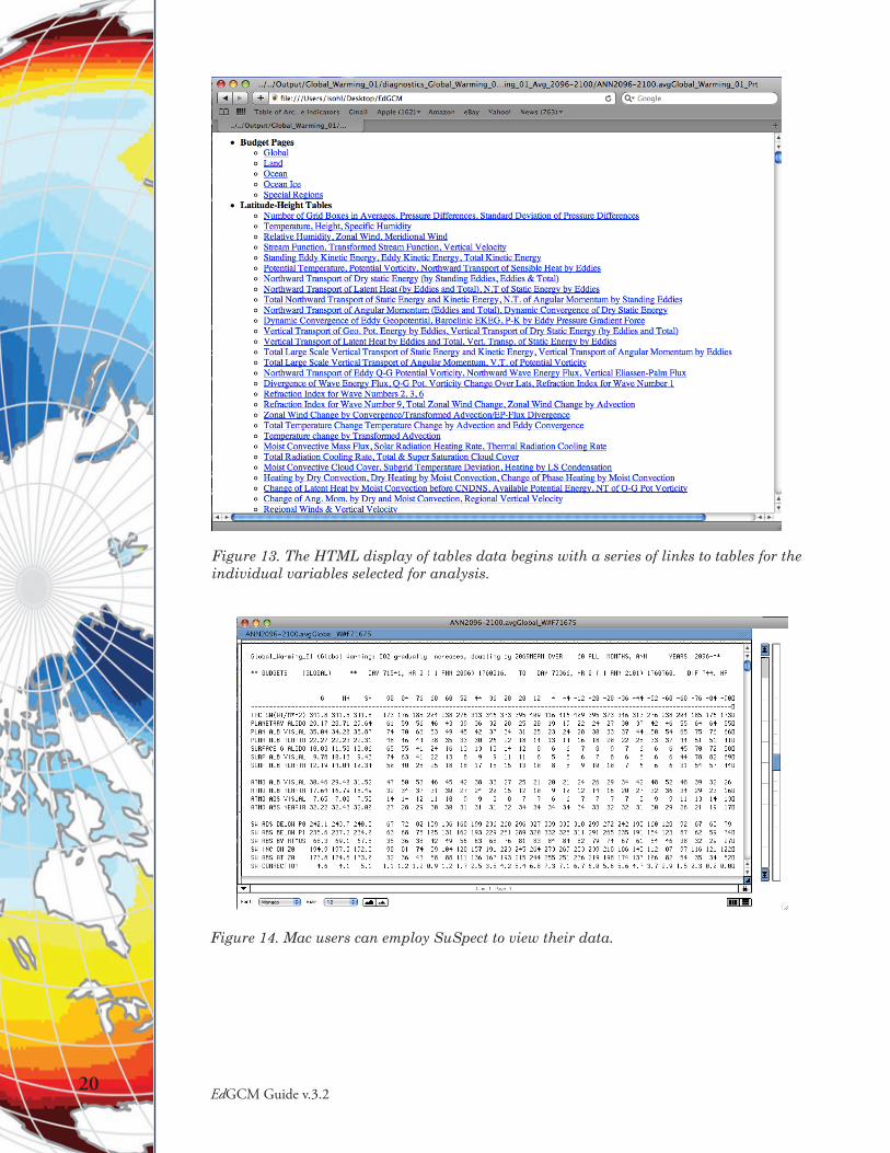
Windows users may choose to view Diagnostic Tables using Microsoft Ex-cel® or, by choosing the files ending in .html, using a web browser. These are very large tables containing information on nearly all the climate vari-ables produced by the GCM, and the html view is perhaps the most ef-ficient way to scan the information because there are links to the specific table for each variable at the top of these files (Figure 13). Mac users have the additional option of viewing the data tables with another prorgram we provide called SuSpect (Figure 14). SuSpect allows users to sychronize the viewing of multiple files for quicker comparison of the results from more than one simulation.
EdGCM Guide v.3.220
Figure 14. Mac users can employ SuSpect to view their data.
Figure 13. The HTML display of tables data begins with a series of links to tables for the individual variables selected for analysis.

EdGCM Guide v.3.2 21
4. Reporting Your Results
1. Return to EdGCM, and select “eJournal” from the Window menu at the top. The eJournal toolbar and window will appear (Figure 15).
Figure 15. The eJournal setup window and its associated toolbar.
An important feature of EdGCM is the ability to share simulation results and interpretations by publishing to a web site easily accessible to others. The entire process is greatly simplified through EdGCM’s eJournal function.
To report results:
2. Note that the eJournal window is divided into sections. Each section of the eJournal (up to a maximum of 20 sections) can be used for either text descriptions or figures. To convert between one type of section to the other, simply click on the button to the left of the section (clicking on a photo button sets up the section for figures; clicking on a text button sets up the section for text).
3. Three additional figures may be added to a given section (for a total of four figures) by clicking the “+” button at the lower right corner of the figure

EdGCM Guide v.3.222
window. Up to two lines of figure caption text, if available, will be visible for each figure in the eJournal setup window, although longer captions will be displayed in their entirety when the eJournal is published to HTML.
4. Images of any size or format can be imported from the Image Browser (Figure 16), which is accessible from the Window menu. Images from the Image Browser may be inserted into an eJournal section by simply dragging and dropping the image into a figure box, such as the one seen in section 2 of the eJournal page in Figure 15.
Figure 16. The Image Browser is a library of photos, graphs, and maps that can be used to illustrate key points for discussion in a student’s eJournal report. The images can be sorted by name, date created or modified, or by theme (e.g., Pliocene images, global warming images). The Image Browser may be added to at any point by students or teachers.
5. To page through multiple pages of the Image Browser, click on the “forward” and “reverse” buttons in the Image Browser toolbar. It is also possible to search for images by name, or sort images by name, creation date, etc.
6. When an eJournal is ready for web publication, return to the filled-out eJournal page and click on the “eJournal to Web” button in the toolbar (see Figure 15). The eJournal page will be converted to an HTML file, which will open automatically in a new window within your default web browser (Figure 17).

EdGCM Guide v.3.2 23
These files can then be published to a school web site or to the student’s own web space for public access. A copy may also be added to the school’s eJournal library, a searchable offline database for the reports.
Figure 17. A published eJournal report.

EdGCM Guide v.3.224
This Agreement is the expression of covenants between the User (“Licensee”), and Columbia University in the City of New York (“Columbia”), regarding current and future versions of software produced by the EdGCM Project. License includes all programs, code, examples, manuals and other documentation included in the release (collectively, “the Software”).
1. Licensee agrees that the Software and the Derivatives will be used solely for non-commercial research or educational purposes. Licensee is not permitted to sell, lease, distribute, transfer, sublicense, or otherwise dispose of the Software and the Derivatives, in whole or in part, for any form of actual or potential commercial gain or consideration;
2. Copyright of the Software is and will remain with The Trustees of Columbia University in the City of New York and/or its employees, consultants and students, and shall at no point transfer to Licensee. Any copyright notices on the Software shall be included on all copies of the Derivatives, or any parts or portions thereof, in any form, manner or substance, which are produced by the Licensee including but not limited to incorporation of the Software into any other program, technical data, documentation, firmware, or other information of the like kind, type or quality;
3. Any externally disseminated publications such as, but not limited to, manuals, technical reports, articles in journals, grant proposals, papers in conference or workshop proceedings, and marketing brochures or advertisements for sale or distribution of products, written in whole or in part by Licensee personnel, including but not limited to employees, consultants or students of Licensee, that are based in any part on the ideas of the Programming Systems Lab or the Software shall acknowledge Mark Chandler and the EdGCM Project at Columbia University, CCSR, using the following citation:
Chandler, M.A., S.J. Richards, and M. Shopsin, 2005: EdGCM: Enhancing climate science education through climate modeling research projects. In Proceedings of the 85th Annual Meeting of the American Meteorological Society, 14th Symposium on Education, Jan. 8-14, 2005, San Diego, CA, pp. P1.5;
4. Licensee acknowledges that the Software is being supplied in an “as is” condition without any support services or future updates or releases. The EdGCM Project at Columbia University may or may not make future updates and releases available to Licensee under this same or another licensing agreement, but Columbia is in no way obligated to do so. If Licensee discovers any defects or limitations in the Software, Licensee is encouraged to inform the EdGCM Project at Columbia University. However, Columbia or its representatives will not necessarily acknowledge or repair any such errors thus reported;
5. Columbia makes no guarantees, warranties or representations of any kind, either express or implied. Furthermore, Columbia disclaims and Licensee waives and excludes any and all warranties of merchantability and any and all warranties of fitness for any particular purpose. Licensee agrees that neither Columbia nor its future, current or former personnel, including but not limited to employees, consultants and students, shall be held to any liability with respect to any claim by Licensee or a third party arising from or on account of the use of the Software
EdGCM Software License for Educational Use

EdGCM Guide v.3.2 25
or the Derivatives, regardless of the form of action; whether in contract or tort, including negligence. In no event will Columbia be liable for consequential or incidental damages of any nature whatsoever;
6. Licensee will guarantee that all actual or potential users of the Software, and all actual or potential producers of the Derivatives, within Licensee organization, or in organizations who have obtained or may obtain the Software or the Derivatives from Licensee, are aware of this agreement and of the terms for using the Software and producing Derivatives.

EdGCM Guide v.3.226
Notes


