EdGCM Workshop Guide | i

Global Climate Modeling Workshop

Teacher Research Academies

Lawrence Livermore National Laboratory

July 7-8, 2010

Instructors:

Dr. Mark Chandler

Dr. Linda Sohl

Sponsored by:

The EdGCM Project

Columbia University in the City of New York

Goddard Institute for Space StudiesNew York, N.Y.

i i | E d GCM W o r k s h o p G u i d E

The EdGCM software suite was developed under the auspices of the EdGCM Project of Columbia University and NASA’s Goddard Institute for Space Studies.

© 2003-2010 Columbia University. All rights reserved.

The EdGCM Project acknowledges the support of the National Science Foundation, Division of Atmospheric Science—Paleoclimate Program

(NSF Award #0231400), and by NASA’s Climate Programs (NASA Award #NNG04GP65G).

EdGCM Workshop Guide | i i i

Contents

the edGCM Workshop Guide

1. Introduction ..............................................................................................1 2. Statement of Expected Outcomes .............................................................2 3. “GCM” – General Circulation Model / Global Climate Model ...............4 4. Global Climate Models Described ............................................................75. Climate Modeling and Global Warming .................................................12

edGCM exercise on Modern Climate Control Runs and Global Warming: Using a GCM to explore Current and Future Climate Change

Part 1: Setting Up a Climate Modeling Experiment .....................................2Part 2: Modern_SpecifiedSST Analysis ........................................................3 Part 3: Modern_PredictedSST Analysis ........................................................3Part 4: Doubled_CO2 Analysis .....................................................................4 Part 5: Global Warming Analysis ..................................................................5

.

i v | E d GCM W o r k s h o p G u i d E

EdGCM Workshop Guide | 1

the edGCM Workshop Guide

Mark A. Chandler, Columbia University, NASA Goddard Institute for Space StudiesAna Marti, University of Wisconsin - Madison, Dept. of Atmospheric and Oceanic Sciences

1. Introduction

Historically, Global Climate Models (GCMs) required supercomputing facilities and skilled programmers to run, and this remains the case for the most complex, cutting-edge models. For this reason, GCMs in the United States have typically been developed at the National Laboratories run by the National Aeronautics and Space Administration (NASA), the National Oceanic and Atmospheric Administration (NOAA) and the National Center for Atmospheric Research (NCAR), where some of the nation’s largest and fastest computing facilities are located. The teams that develop GCMs include scientists from a wide variety of disciplines: atmospheric scientists, physicists, geoscientists, oceanographers, mathematicians, biologists, botanists and, of course, computer scientists.

Recently, advances in computing technology have made it possible for some GCMs to run on less expensive workstations and even on desktop PCs, making them available for use in schools and accessible by a broader community of researchers, teachers and students.

This unit will take advantage of this new accessibility to GCMs to learn more about the global warming problem and specifically about the effects of carbon dioxide increase (the major anthropogenic greenhouse gas) on future climate.

In order to reach this goal, we will use the EdGCM software suite, which is an excellent tool for teaching and learning climate change. The numerical model allows students to construct their knowledge around climate change as they explore on their own how different components of the climate system contribute in determining our climate. The use of EdGCM in the classroom also provides the opportunity to students to understand and use the methods and tools utilized by scientists in their research.

2 | E d GCM W o r k s h o p G u i d E

2. statement of expected outcomes

the edGCM Project: overarching Goals

1. Allow teachers to run a 3-D global climate model (GCM) on a desktop computer, encouraging students to participate in the full scientific process employed by researchers including: experiment design, running simulations, analyzing data and reporting results.

2. Facilitate collaborations within the education community and between students, teachers and research scientists so that students become familiar with the role that teamwork plays in scientific research.

the edGCM Project: specific objectives

By participating in the workshop session, teachers will achieve the following:

The Scientific Process: A Climate Scientist’s Experience

• Participants will gain an understanding of the typical scientific process climate scientists go through when using climate models: developing a hypothesis, designing an experiment, running a computer simulation, analyzing model output (i.e. post-processing raw computer data and using scientific visualization techniques), creating written reports in the form of scientific manuscripts (i.e. describing experiment design, results and conclusions using text and images), and publishing reports (to the web).

• Learn how EdGCM has been developed specifically for desktop computers to allow its users to become familiar with scientific tools that are normally available only at national labs.

Global Climate Models (GCMs)

• Participants will gain an understanding of the history and theoretical aspects of Global Climate Models and how they are currently used to enable research scientists, teachers and students to examine earth’s past, present, and future climates.

Concepts of Modeling

• Participants will gain an understanding of the step-by-step procedures that are used by climate model research scientists in setting up an experiment, conducting control runs, inputting variables, and producing typical output products.

EdGCM Workshop Guide | 3

EdGCM Basics

• Participants will learn what level of computer resources are required to accomplish specific experiments and learning objectives and will understand how to organize a climate modeling unit that fits their schools resources.

• Participants will acquire the basic knowledge and skills required to use the EdGCM software suite in the classroom through guided hands-on computer activities.

EdGCM Exercise on Global Warming

• Participants will gain an understanding of how Global Climate Models are used to investigate global warming. Workshop members will set up, run, analyze, and report on basic global warming experiments using the EdGCM software suite.

EdGCM Features for Teacher Use Only: Administrative Features

• Participants will gain an understanding of various technical details and administrative procedures regarding EdGCM software installation, computer hard disk usage and maintenance, database backup and security issues.

The EdGCM Website (http://edgcm.columbia.edu): Support and On-line Features

• Participants will become informed about the features of the EdGCM website that offer online support for members of the EdGCM community through the EdGCM Support Forums: http://forums.edgcm.columbia.edu

4 | E d GCM W o r k s h o p G u i d E

3. “GCM”General Circulation Model / Global Climate Model

GCMs are Process Models - simulations are based on fundamental physical equations and, therefore, GCM output is examined not only to establish a Cause and Effect relationship, but to explore the many feedback mechanisms by which the Earth’s climate system operates. The “Primitive Equations” calculate Temperature (T), Pressure (P), Winds (U,V,W) and Specific Humidity (Q), and a wide variety of empirically-based or theoretically-based equations are used to parameterize other processes (e.g., cloud formation, radiation interactions) that are not described explicitly via the fundamental physical equations.

In the climate system there is rarely a simple cause and effect relationship between phenomena. Instead, forcing mechanisms set into motion a series of feedback processes that eventually alter the equilibrium of the climate. Often, the feedbacks themselves are more powerful agents of change than the original forcing.

As an example, at right is an illustration of the connections between the positive feedbacks associated with ice/snow albedo, terrestrial snow and vegetation, which contribute to high-latitude warming, and the negative feedbacks associated with clouds that can alleviate such the warming. This web of feedback effects can be driven by any “simple” cause that affects the net radiation absorbed by the atmosphere – from an explosive volcanic eruption to emissions from fossil fuel burning to short-term solar variability.

Image credit: Hugo Ahlenius, UNEP/GRID-Arendal)

EdGCM Workshop Guide | 5

Using a GCM on a supercomputer: Model rundecks

Global_Warming_01.R Model II 2/11/05

Creator: Mark Chandler

Comments: based on Modern control run using Model II, which uses predicted SST with deep ocean diffusionInitial CO2 = 315.4 Increasing CO2 trend is linear with 0.5 ppm increase per year through 2000 then an additional 1.0%per year exponential increase from 2000 through 2100. This yields a doubled-CO2(i.e. double the 1958 value = 629.8ppm) around the year 2062.All other greenhouse gases are held fixed at 1958 values to match the control run

Model version: Model=Model II 1.0.7 Grid=8x10x9

Data and input files: 9=NOV1960.rsfModern_DeepOcean, 15=O8X10.250MLD, 17=otspec_Spec_A3_v106_1.00 19=CD8X10, 21=RTAU.G25L15, 22=RPLK25, 23=V8X10, 25=Z1OMAX.8X10.250M 26=Z8X101, 29=REG8X10, 62=ED8X10

Label and namelist:Global_Warming_01 (Global Warming: CO2 gradually increases, doubling by 2069)

&INPUTZ GEOMETRY=’8x10’, TAUI=507336., IYEAR=1900, KOCEAN=2,SRCOR=0.9644674710387354244, S0X=1366.6198,CO2=314.9,USET=0.,TAUE=1760760., USESLP=0.,KCOPY=2, ISTART=3,KCHECKTAUX=1,IRAND=123456789,NDPRNT=-1, KDIAG=0,9,9,9,9,9,9,9,9, TAUE=507337., OMEGT=282.9,OBLIQ=23.44,ECCN=0.0167, &END

&FORCINGS KTRENDEXT=1, ICO2DATA=200,ICO2DATASTART=1957,ICO2DATAEND=2100, ZN2O=0.2908, CH4=1.224, F11=0.0076,

F12=0.0296, &END

Unix scripts, like this model rundeck, are used to initiate climate simulations on supercomputers and powerful workstations. They are efficient for scientists and programmers, but they assume a great deal of prerequisite knowledge regarding the computer model and require that the user have significant computer programming skills.

6 | E d GCM W o r k s h o p G u i d E

Using a GCM on a desktop computer: edGCM

EdGCM Workshop Guide | 7

4. Global Climate Models Described

the nAsA/GIss Global Climate Model

The climate model used by the EdGCM software was developed at NASA’s Goddard Institute for Space Studies (NASA/GISS). This type of 3-dimensional computer model is known as a grid-point Global Climate Model (GCM). A grid point GCM divides the atmosphere into a series of discrete grid cells. EdGCM’s model grid has 7776 grid cells in the atmosphere, with each horizontal column corresponding to 8° latitude by 10° longitude and containing 9 vertical layers. The computer model numerically solves fundamental physical equations, which describe the conservation of mass, energy, momentum, and moisture in each cell, while taking into account the transport of quantities between cells. It then uses the Ideal Gas Law to relate pressure to temperature, two of the most important climate variables. Parameterizations, based on empirical data or simplified physical hypotheses, are used to calculate quantities that are not handled by the fundamental equations, or which occur at spatial scales that are finer than the scale of the model’s grid. For example, plants, convective clouds, and river run-off are all parameterized in GCMs (see below for more information about parameterizations).

GCMs explained

At the heart of a GCM is a model of the Earth’s atmosphere. There are five fundamental physical equations that are used to describe the evolving state of the atmosphere: the conservation of mass, conservation of energy, conservation of momentum, conservation of moisture and the ideal gas law (to approximate the equation of state).

There are two basic forms of the fundamental equations used to simulate the atmosphere in global climate models. These define two distinct families of models: Cartesian grid point GCMs and spectral GCMs. In a Cartesian grid point model the atmosphere is divided horizontally and vertically into a series of grid cells. The equations are solved for each cell in the grid, while taking into account the transport

8 | E d GCM W o r k s h o p G u i d E

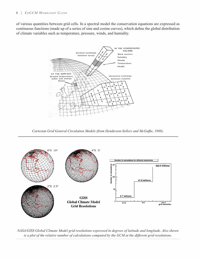
of various quantities between grid cells. In a spectral model the conservation equations are expressed as continuous functions (made up of a series of sine and cosine curves), which define the global distribution of climate variables such as temperature, pressure, winds, and humidity.

Cartesian Grid General Circulation Models (from Henderson-Sellers and McGuffie, 1988).

NASA/GISS Global Climate Model grid resolutions expressed in degrees of latitude and longitude. Also shown is a plot of the relative number of calculations computed by the GCM at the different grid resolutions.

 

 

EdGCM Workshop Guide | 9

The main components of the atmospheric portion of a GCM are those that represent the atmospheric dynamics and the interactions of the Sun’s radiation with the planet. The dynamics calculations help define the general circulation of the atmosphere as well as smaller-scale eddy circulations, such as the cyclonic storm systems that control much of the weather in the mid-latitudes. The radiation calculations determine the energy balance of the Earth by evaluating the reflection and absorption of solar radiation by the surface and atmosphere, and by the remittance of thermal energy back to space. The radiation calculations in a GCM must take into account cloud thickness and cloud distribution (horizontal and vertical), surface conditions (land vs. ocean, topography, vegetation types, snow and ice cover), and all significant greenhouse gases and aerosols.

Schematic illustration of the physical components of the climate system represented at each model grid cell (adapted from Hansen et al., 1990).

While climate models of varying complexity exist, defining simple vs. complex climate models is not necessarily straightforward. That’s because climate models may be considered more complex if they incorporate additional dimensions, increase the spatial or temporal resolution at which calculations are applied, represent the physics more completely, or incorporate parameterizations that describe additional components of the climate system (e.g., oceans, vegetation, ground hydrology, ice sheets, the carbon cycle, etc.). Perhaps the most important of these additions to the atmospheric model are the coupling of the atmospheric GCMs to 3-D ocean circulation models.

10 | E d GCM W o r k s h o p G u i d E

Ocean General Circulation Models

Global Climate Models have evolved over time to include more and more of the physical and chemical components of the climate system. Many characteristics of the Earth that were supplied as boundary conditions in earlier models can now be simulated in the latest models. Moreover, as new scientific studies advance our understanding of the Earth’s physical environment, climate models incorporate the new findings by altering or adding to existing calculations. Ultimately, this allows climate models to describe the climate system in greater detail and with improved precision.

Probably the most significant change to the traditional structure of global climate models was the advent of models that coupled an atmospheric GCM to a 3-dimensional ocean GCM. 3-D ocean models have been under development for nearly as long as atmospheric models and some of the most important experiments, commanding the most computing resources, have employed coupled ocean-atmosphere GCMs for a decade or more. However, coupled GCMs have only recently become a standard for use in simulating the broad array of climate experiments underway that study everything from climates of the geologic past to the many scenarios that seek to represent the potential states of future climate. Some of the lag in incorporating fully dynamic oceans into global climate models has been due to the added pressure on computational resources that the ocean calculations represent: the ocean’s cover nearly two-thirds of the surface of the Earth; they circulate slowly compared to the atmosphere, requiring longer simulations; on average key features in the ocean (e.g. eddies, western boundary currents, upwelling, and deep water formation) occur at finer scales than analogous atmospheric circulation phenomena (which tend to average 1000’s of kilometers instead of 10’s of kilometers as with the oceans). On the other hand, much of the delay in developing and applying coupled ocean-atmosphere models was simply related to the fact that we knew precious little about the how physical oceans operated. The past two decades has seen an astounding increase in our understanding Earth’s oceans and how they operate over both short and long time scales. It may be that the ultimate reason that coupled oceans models have become a standard component of global climate models is because they have simply reached a point where scientists have much more confidence in the results they produce.

ClimateModelParameterizations

Climate models built for predictive purposes would, ideally, be derived entirely on fundamental laws of nature. For example, the ideal gas law makes it possible for a GCM to always determine an exact relationship between temperature (T) and pressure (p), which are two critical variables used in the determination of the energy balance and movement of the atmosphere. However, our knowledge of the exact workings of many of the processes in the climate system is still limited. Furthermore, many of those processes operate on scales too fine for existing computers to simulate. Therefore, models simulate a number of the key components of the climate system by using series of calculations that are derived from statistical or empirical relationships between variables. These types of calculations are called parameterizations and they range from simple one-line equations (for example, an equation that instructs a portion of an ocean grid cell to freeze at a fixed temperature based on a constant salinity) to highly complex sequences of equations that describe cloud processes, vegetation, continental ice sheets, atmospheric chemistry, ground hydrology, and more. In fact, many parameterizations are themselves models that are designed to simulate just one part of the climate system. However, when carefully linked to an atmospheric GCM, an ocean model, and other parameterizations, they make up a virtual Earth Climate System Model. Such models that couple together atmospheric and oceanic GCMs with complex parameterizations are increasingly becoming the successors to GCMs.

EdGCM Workshop Guide | 11

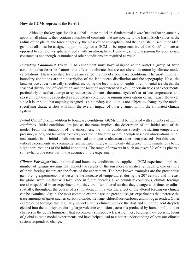
How do GCMs represent the earth?

Although the key equations in a global climate model are fundamental laws of nature that presumably apply on all planets, they contain a number of constants that are specific to the Earth. Such values as the radius of the planet, the force of gravity, the mass of the atmosphere, and the R constant used in the ideal gas law, all must be assigned appropriately for a GCM to be representative of the Earth’s climate as opposed to some other spherical body with an atmosphere. However, simply assigning the appropriate constants is not enough. A number of other conditions are required as well:

Boundary Conditions: Every GCM experiment must have assigned at the outset a group of fixed conditions that describe features that effect the climate, but are not altered in return by climate model calculations. These specified features are called the model’s boundary conditions. The most important boundary conditions are the description of the land-ocean distribution and the topography. Next, the land surface cover is usually specified, including the locations and heights of continental ice sheets, the seasonal distribution of vegetation, and the location and extent of lakes. For certain types of experiments, particularly those that attempt to reproduce past climates, the annual cycle of sea surface temperatures and sea ice might even be specified as a boundary condition, assuming observations of such exist. However, since it is implicit that anything assigned as a boundary condition is not subject to change by the model, specifying characteristics will limit the overall impact of other changes within the simulated climate system.

Initial Conditions: In addition to boundary conditions, GCMs must be initiated with a number of initial conditions. Initial conditions are just as the name implies, the description of the initial state of the model. From the standpoint of the atmosphere, the initial conditions specify the starting temperature, pressure, winds, and humidity for every location in the atmosphere. Though based on observations, small inaccuracies in the initial conditions can lead to unique results as an experiment proceeds. For this reason, critical experiments are commonly run multiple times, with the only difference in the simulations being slight perturbations of the initial conditions. The range of answers in such an ensemble of runs places a somewhat crude error-bar on the accuracy of the experiment.

Climate Forcings: Once the initial and boundary conditions are supplied a GCM experiment applies a number of climate forcings that impact the results of the run more dramatically. Usually, one or more of these forcing factors are the focus of the experiment. The best-known examples are the greenhouse gas forcing experiments that describe the increase of temperatures during the 20th century and forecast the global warming that will take place in future decades. Like boundary conditions, climate forcings are also specified in an experiment, but they are often altered so that they change with time, or adjust spatially, throughout the course of a simulation. In this way the effect of the altered forcing on climate can be examined. Again, the most common example are the greenhouse gas experiments that increase the trace amounts of gases such as carbon dioxide, methane, chlorofluorocarbons, and nitrogen oxides. Other examples of forcings that regularly impact Earth’s climate include the dust and sulphuric acid droplets ejected into the atmosphere during large volcanic explosions, aerosols produced by human pollution, or changes in the Sun’s luminosity that accompany sunspot cycles. All of these forcings have been the focus of global climate model experiments and have helped lead to a better understanding of how our climate system responds to change.

12 | E d GCM W o r k s h o p G u i d E

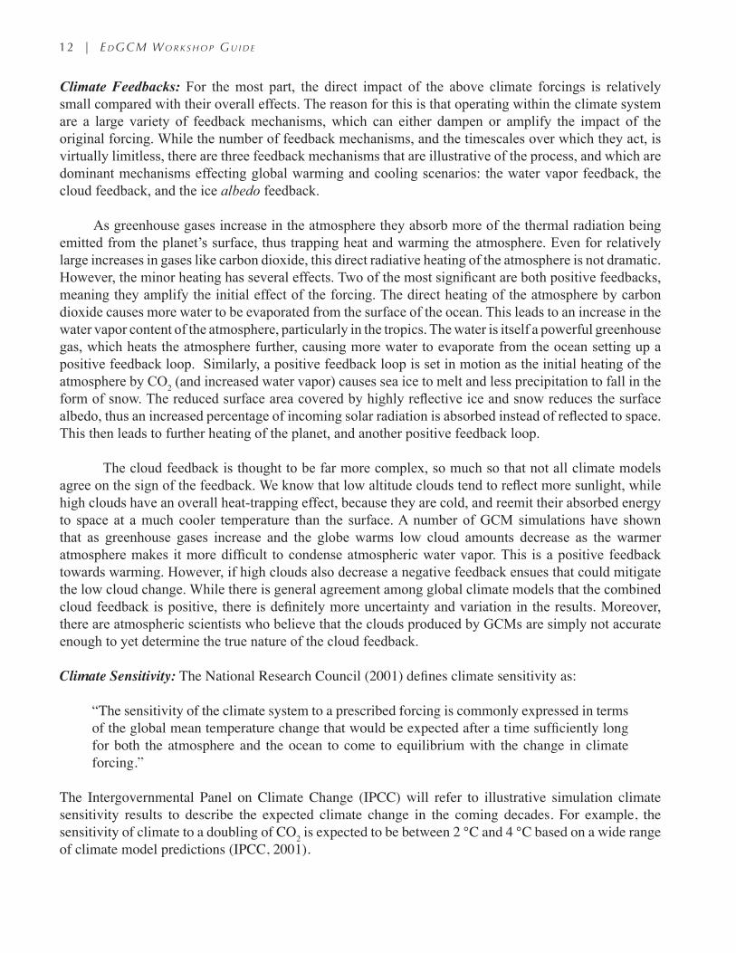
Climate Feedbacks: For the most part, the direct impact of the above climate forcings is relatively small compared with their overall effects. The reason for this is that operating within the climate system are a large variety of feedback mechanisms, which can either dampen or amplify the impact of the original forcing. While the number of feedback mechanisms, and the timescales over which they act, is virtually limitless, there are three feedback mechanisms that are illustrative of the process, and which are dominant mechanisms effecting global warming and cooling scenarios: the water vapor feedback, the cloud feedback, and the ice albedo feedback.

As greenhouse gases increase in the atmosphere they absorb more of the thermal radiation being emitted from the planet’s surface, thus trapping heat and warming the atmosphere. Even for relatively large increases in gases like carbon dioxide, this direct radiative heating of the atmosphere is not dramatic. However, the minor heating has several effects. Two of the most significant are both positive feedbacks, meaning they amplify the initial effect of the forcing. The direct heating of the atmosphere by carbon dioxide causes more water to be evaporated from the surface of the ocean. This leads to an increase in the water vapor content of the atmosphere, particularly in the tropics. The water is itself a powerful greenhouse gas, which heats the atmosphere further, causing more water to evaporate from the ocean setting up a positive feedback loop. Similarly, a positive feedback loop is set in motion as the initial heating of the atmosphere by CO2 (and increased water vapor) causes sea ice to melt and less precipitation to fall in the form of snow. The reduced surface area covered by highly reflective ice and snow reduces the surface albedo, thus an increased percentage of incoming solar radiation is absorbed instead of reflected to space. This then leads to further heating of the planet, and another positive feedback loop.

The cloud feedback is thought to be far more complex, so much so that not all climate models agree on the sign of the feedback. We know that low altitude clouds tend to reflect more sunlight, while high clouds have an overall heat-trapping effect, because they are cold, and reemit their absorbed energy to space at a much cooler temperature than the surface. A number of GCM simulations have shown that as greenhouse gases increase and the globe warms low cloud amounts decrease as the warmer atmosphere makes it more difficult to condense atmospheric water vapor. This is a positive feedback towards warming. However, if high clouds also decrease a negative feedback ensues that could mitigate the low cloud change. While there is general agreement among global climate models that the combined cloud feedback is positive, there is definitely more uncertainty and variation in the results. Moreover, there are atmospheric scientists who believe that the clouds produced by GCMs are simply not accurate enough to yet determine the true nature of the cloud feedback.

Climate Sensitivity: The National Research Council (2001) defines climate sensitivity as:

“The sensitivity of the climate system to a prescribed forcing is commonly expressed in terms of the global mean temperature change that would be expected after a time sufficiently long for both the atmosphere and the ocean to come to equilibrium with the change in climate forcing.”

The Intergovernmental Panel on Climate Change (IPCC) will refer to illustrative simulation climate sensitivity results to describe the expected climate change in the coming decades. For example, the sensitivity of climate to a doubling of CO2 is expected to be between 2 °C and 4 °C based on a wide range of climate model predictions (IPCC, 2001).

EdGCM Workshop Guide | 13

5. Climate Modeling and Global Warming

Introduction

At the current rate of increase, by the time today’s high school students become grandparents the amount of carbon dioxide in the Earth’s atmosphere will be higher than it has been at anytime during the previous 50 million years of Earth history. Most, if not all, of this increase will be due to human influences – primarily the burning of fossil fuels in automobiles and power generating plants. Why do scientists care so much about this invisible gas that makes up only a fraction of a percent of the molecules in the Earth’s atmosphere? The answer is that carbon dioxide is the most prevalent greenhouse gas on our planet. Its presence in our atmosphere helps make the surface of the Earth warm enough to inhabit, but its rapid increase is likely to lead to globally averaged temperatures that are warmer than any experienced on Earth since before the evolution of the human species. Many people are concerned about how this “global warming” could impact the environment, the economy, and the lives of people all over the world. Scientists therefore, need to learn more about the details of this real-world experiment that we are conducting within our atmosphere. How much warming will occur during the next several decades? Will it be evenly distributed, or will some locations warm more than others? Will the temperature increase gradually, or will there be abrupt shifts in the climate? And, how will warming temperatures influence other climate phenomena, such as rain, snow and winds?

In order to explore these questions, and hopefully answer them with a high degree of accuracy, climate scientists are increasingly relying on large computer models of the earth’s climate system. The most complex, and most relied upon climate models are collectively known as Global Climate Models.

Global climate models are computer programs that simulate the Earth’s climate system in three-dimensions and are commonly referred to by their acronym “GCM”. Computer global climate models, or GCMs, are used extensively in the effort to predict future climate changes, such as the impacts of increasing greenhouse gases, and they are employed by geoscientists to explore the average state and variability of past climates, from the climate of the 20th century to that of the ancient Earth. In addition to their use in forecasting realistic, whole-earth climate changes of the past, present and future, global climate simulations help scientists examine the sensitivity of the climate system to altered internal and external forcings. Examples of sensitivity tests that scientists might try include examining how the climate reacts to random changes in the Sun’s energy output or calculating how much global temperature increases if atmospheric carbon dioxide is doubled. A computer climate simulation allows scientists to isolate individual factors, and then analyze their impact on discrete components of the climate system. For example, climate simulations can help determine the effect of increased CO2 on things that are important in our society such as the average start date of the growing season, the impact of solar variability on tropical precipitation, or the role of ocean heat transport in the intensity of mid-latitude storms.

Of course, GCMs are not perfect crystal balls. After all, no matter how complex their representations of climate, the climate system itself is many times more complex. However, they are deeply dependent on fundamental laws of nature (as opposed to statistical correlations) and modern GCMs do an amazing job at simulating observed and historical climate change. Perhaps most important is that they provide us with an opportunity to explore and comprehend the processes of the Earth’s climate system in four dimensions - three in space and one in time. Understanding the relationship between Earth observations and the processes that led to them gives us an improved capacity for prediction, which can then be used to aid

14 | E d GCM W o r k s h o p G u i d E

policymakers, ecologists, public health officials, natural resource departments, industries or populations effected by climate change, and many others.

Weather and Climate: Important Distinctions

Before delving more deeply into the subject of climate science it is important to understand the differences between weather and climate. Simply stated, weather describes the changing state of the atmosphere at a particular location over time intervals of short duration - minutes to perhaps no longer than a few weeks. It consists of atmospheric elements such as temperature, humidity, air pressure, wind speed and wind direction, precipitation, cloud cover and cloud types, and visibility. Hurricanes, thunderstorms, tornadoes, blizzards, rainbows, and fog also are a part of everyday weather. Climate, on the other hand, is time-averaged weather and is characterized by statistics that help describe the mean weather conditions and variations at a single place, region, or worldwide for a particular period of time – a month, a year or over much longer intervals.

Despite continuing marvelous advances weather remains difficult to predict beyond a one-week period. Climate, on the other hand, tends to be far more “behaved” and thus more predictable. For instance, most of us could fairly easily predict that the next five Augusts in New York will be warmer on average than the average temperature of the next five Mays, or that next five Mays will be wetter than next five Augusts. The fact that climate uses longer averages to describe phenomena and that it deals with large-scale patterns which tend to repeat themselves from year to year make it more predictable. However, climate becomes more difficult to predict when forces beyond the normal range of variability alter the characteristic physical responses of the climate system itself. This type of situation is essentially what climate scientists now face, in light of the significant increase in carbon dioxide and other greenhouse gases in the atmosphere contributed by industrial growth and associated fossil fuel burning over the past century.

Greenhouse Gases: sources, sinks, and Destructive Mechanisms

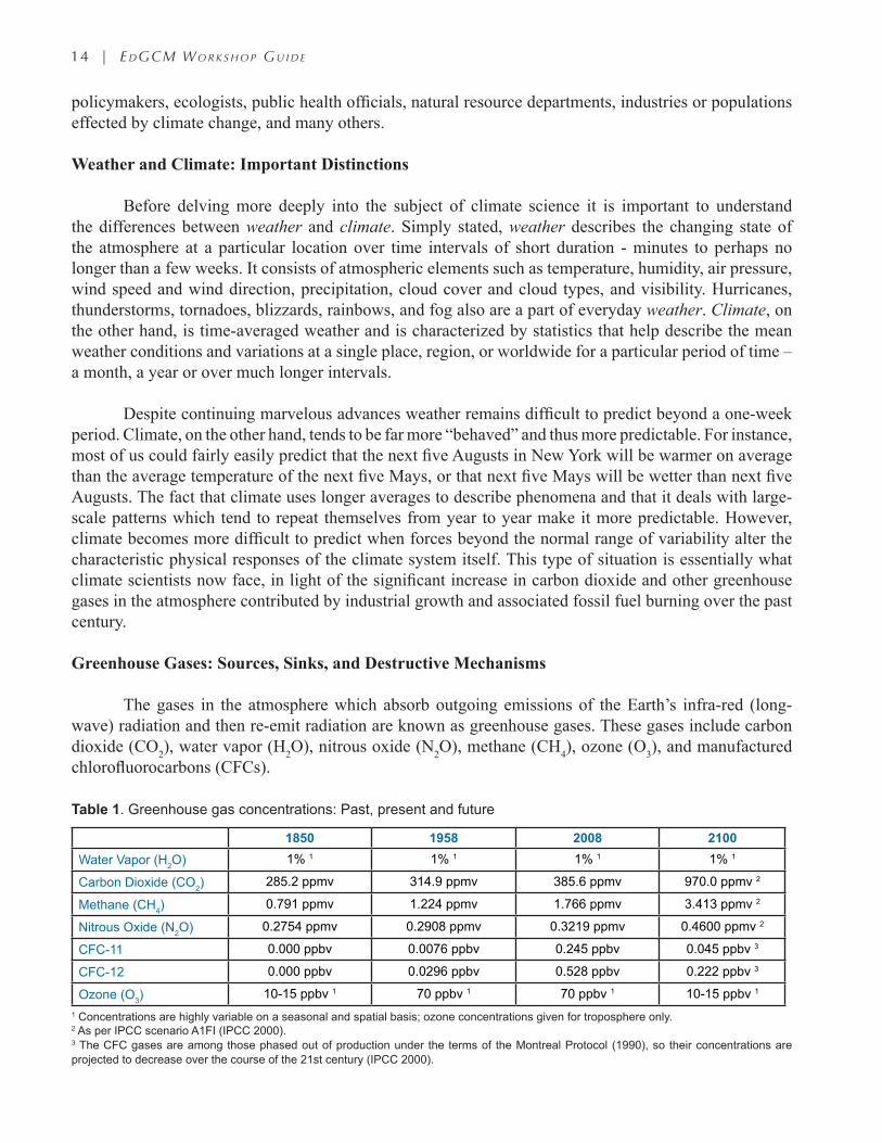
The gases in the atmosphere which absorb outgoing emissions of the Earth’s infra-red (long-wave) radiation and then re-emit radiation are known as greenhouse gases. These gases include carbon dioxide (CO2), water vapor (H2O), nitrous oxide (N2O), methane (CH4), ozone (O3), and manufactured chlorofluorocarbons (CFCs).

Table 1. Greenhouse gas concentrations: Past, present and future

1850 1958 2008 2100Water Vapor (H2O) 1% 1 1% 1 1% 1 1% 1

Carbon Dioxide (CO2) 285.2 ppmv 314.9 ppmv 385.6 ppmv 970.0 ppmv 2

Methane (CH4) 0.791 ppmv 1.224 ppmv 1.766 ppmv 3.413 ppmv 2

Nitrous Oxide (N2O) 0.2754 ppmv 0.2908 ppmv 0.3219 ppmv 0.4600 ppmv 2

CFC-11 0.000 ppbv 0.0076 ppbv 0.245 ppbv 0.045 ppbv 3

CFC-12 0.000 ppbv 0.0296 ppbv 0.528 ppbv 0.222 ppbv 3

Ozone (O3) 10-15 ppbv 1 70 ppbv 1 70 ppbv 1 10-15 ppbv 1

1 Concentrations are highly variable on a seasonal and spatial basis; ozone concentrations given for troposphere only.2 As per IPCC scenario A1FI (IPCC 2000).3 The CFC gases are among those phased out of production under the terms of the Montreal Protocol (1990), so their concentrations are projected to decrease over the course of the 21st century (IPCC 2000).

EdGCM Workshop Guide | 15

The “greenhouse” effect of these gases comes from their ability to absorb frequencies that lie in the infra-red part of the spectrum, which is the same range in which the Earth radiates energy to space. The greenhouse gases can thus capture much of this energy, with the end result that the atmosphere is warmer than it would be if these gases were not present.

Carbon dioxide is released from the interior of the Earth through volcanic eruptions, and is produced by animal respiration, soil processes, combustion of carbon compounds and oceanic evaporation (CO2 sources). At the same time, carbon dioxide is dissolved in the oceans and absorbed by vegetation during photosynthesis (CO2 sinks). This constant exchange between sources and sinks is known as the global carbon cycle, and it is known to operate over short (up to 103 years) as well as long (105 to 106 years) time scales. Anthropogenic (human-produced) emissions from the burning of fossil fuels and tropical deforestation are currently exceeding the short-term carbon cycle’s ability to re-absorb CO2 via sinks, so the atmospheric concentration of CO2 is continuing to rise.

The global carbon cycle, including human contributions to sources and sinks.

Image credit: Inez Fung, UC-Berkeley.

Trend of CO2 concentrations. Measured and reconstructed CO2 values are shown for 1850-2008; IPCC projections for various emission scenarios are shown for 2009-2100. Scenarios A1FI and A2 represent possible CO2 levels given continued reliance on fossil fuel consumption and minimal or no mitigation effort. See IPCC (2000) for a detailed explanation of the assumptions and considerations involved for each scenario.

16 | E d GCM W o r k s h o p G u i d E

Water vapor, which has the greatest greenhouse effect in the atmosphere, is released into the atmosphere from open water surfaces such as oceans and lakes through the process of evaporation and to a much lesser extent from land surfaces and vegetation by means of evaporation and evapo-transpiration. Water vapor experiences a change of state, from gas to liquid, through the process of condensation. Most water vapor is found in the troposphere. Its concentration is established through internal mechanisms of the climate system and is not appreciably affected in a direct way by human actions. However, if greenhouse gases added by man cause the planet to warm, additional evaporation from the oceans would lead to increased water vapor in the atmosphere, amplifying the greenhouse effect.

The global water cycle.

Image credit: NASA GSFC Energy and Water cycle Study (NEWS).

nitrous oxide is formed by numerous reactions of microorganisms in the oceans and soils. It is also produced by various anthropogenic actions that include industrial combustion, vehicle exhausts, the burning of biomass and the use of chemical fertilizers. N2O is destroyed in the stratosphere by photochemical reactions driven by sunlight.

Methane is a very significant greenhouse gas. Current emissions of CH4 are primarily due to the growing of rice, the digestive processes of grazing cattle, the mining of coal and drilling of oil and natural gas deposits, and decomposition of natural wastes in landfills. Methane is destroyed in the troposphere through its reaction with free hydroxyl (OH) radicals:

CH4 + OH → CH3 + H2O

ozone (O3), which is produced naturally in the stratosphere, is mixed into the lower atmosphere in small quantities. When some oxygen molecules (O2) absorb solar ultraviolet radiation they split to yield two oxygen atoms. These freed atoms may then combine with remaining O2 molecules to form ozone:

O2 + O → O3

EdGCM Workshop Guide | 17

During the last century, some additional ozone has been produced near the surface by the action of sunlight on polluted air that results from emissions of motor vehicles, the burning of fossil fuels in power plants, and biomass burning.

The main cause of ozone depletion in the stratosphere is reaction of the O3 with man-made chemicals like chlorofluorocarbons (CFCs, which are further discussed below). CFCs rise into the stratosphere from the surface and chlorine is released through reaction with ultraviolet radiation. Chlorine, in turn, reacts with the highly unstable ozone, causing its destruction.

Chlorofluorocarbons (CFCs) have been used in refrigerants and aerosol propellants and have also been found in industrial pollution. They are composed of carbon, chlorine and fluorine molecules. CFC concentration steadily rose from the time of its development in the late 1920’s until production ended in January 1996. CFCs have the potential to significantly affect climate because of their considerable radiative forcing effects (hundreds to thousands of times greater than CO2) and century-long atmospheric lifetimes. CFCs were replaced by hydrofluorocarbons or HFCs, which also have a potent greenhouse effect, but do not have the atmospheric longevity of CFCs. Both groups of gases have been or are being phased out of use under the terms of the Montreal Protocol treaty first signed in 1990, which was designed to protect the ozone layer.

.

18 | E d GCM W o r k s h o p G u i d E

References

Hansen, J.E., Lacis, A.A., and Ruedy, R.A., 1990. Comparison of solar and other influences on long-term climate. In Climate Impact of Solar Variability, NASA CP-3086. K.H. Schatten and A. Arking, Eds. National Aeronautics and Space Administration, pp. 135-145.

Henderson-Sellers, A., and McGuffie, K., 1988. A Climate Modelling Primer. New York, John Wiley & Sons, Inc., 234 p.

IPCC, 2000. Special Report on Emissions Scenarios: A Special Report of Working Group III of the Inter-governmental Panel on Climate Change. Cambridge, UK: Cambridge University Press. Available at http://www.ipcc.ch/ipccreports/sres/emission/index.php?idp=0.

IPCC, 2001. Climate Change 2001: The Scientific Basis. Cambridge: Cambridge University Press. Avail-able at http://www.grida.no/publications/other/ipcc_tar/.

National Research Council, Committe on the Science of Climate Change, 2001. Climate Change Sci-ence: An Analysis of Some Key Questions. Washington, D.C., National Academy Press, 42 p. Avail-able at http://www.nap.edu/catalog/10139.html.

Additional resources on the web

Global Warming Basics, by the Pew Center on Global Climatehttp://www.pewclimate.org/global-warming-basics

NASA/GISS Surface Temperature Analysis (GISTEMP)http://data.giss.nasa.gov/gistemp/

Understanding Climate Change, by the University Corporation for Atmospheric Research (UCAR)http://www2.ucar.edu/news/backgrounders/understanding-climate-change-global-warming

Climate Literacy: The Essential Principles of Climate Science, by NOAAhttp://www.climate.noaa.gov/index.jsp?pg=/education/edu_index.jsp&edu=literacy

RealClimate Blog - An informal venue for discussing climate topics in-depth with climate scientistshttp://www.realclimate.org

Online companion to the book The Discovery of Global Warming, by Spencer Weart - Looks at the his-tory of climate change research and provides in-depth discussion of key topics.http://www.aip.org/history/climate/

EdGCM Workshop Guide | 19

EdGCM Exercise: Modern Control Runs and Global Warming

EdGCM Exerc i se | 1

EdGCMExerciseonModernClimateControlRunsandGlobalWarmingUsing a GCM to explore Current and Future Climate Change

Mark A. Chandler, Columbia University, Goddard Institute for Space StudiesAna Marti, University of Wisconsin - Madison, Dept. of Atmospheric and Oceanic Sciences

outline

Part 1: Setting Up a Climate Modeling Experiment

Part 2: Modern_SpecifiedSST Analysis- Explain simulation Modern_SpecifiedSST- Visualize the data- Examine climate basics (surface air temperature, zonal average (pole to equator gradient),

seasonal temperature maps, global annual precipitation patterns, temperatures and zonal winds in vertical profile

Part 3: Modern_PredictedSST Analysis - Explain simulation Modern_PredictedSST- Visualize the data - Compare with Modern_SpecifiedSST

Part 4: Doubled_CO2 Analysis- Explain simulation Doubled_CO2- Visualize the data- Compare with Modern_PredictedSST (Equilibrium Climate)

Part 5: Global Warming Analysis - Explain simulation Global_Warming- Visualize the data- Compare with Modern_PredictedSST- Explain global warming impacts and feedback mechanisms

• Surface air temperature• Ice-albedo feedback (snow and ice cover)• Cloud albedo feedback (low cloud cover)• Water vapor• Precipitation and Evaporation (Moisture balance)

2 | E d GCM E x E r C i s E

Part1:SettingUpaClimateModelingExperiment

1.DuplicateanexistingrunfromtherunlistandopenSetupSimulations2.SetRequiredfieldsinthegeneralinformationsection

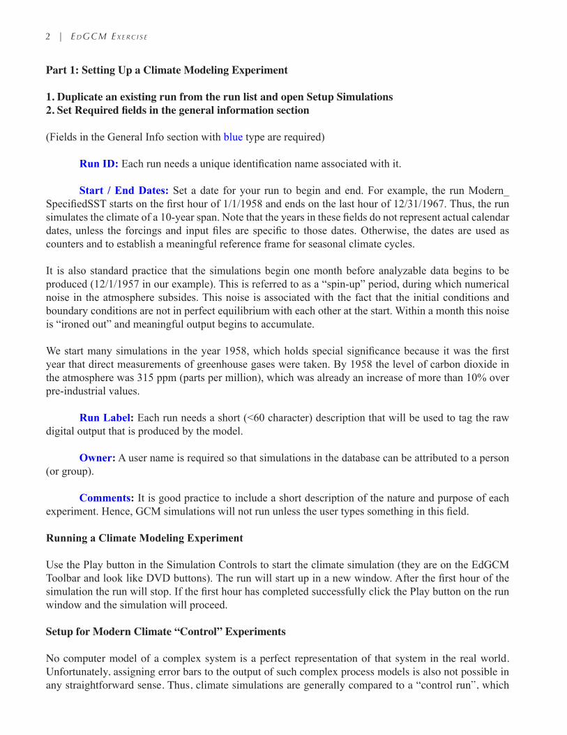
(Fields in the General Info section with blue type are required)

Run ID: Each run needs a unique identification name associated with it. start / end Dates: Set a date for your run to begin and end. For example, the run Modern_SpecifiedSST starts on the first hour of 1/1/1958 and ends on the last hour of 12/31/1967. Thus, the run simulates the climate of a 10-year span. Note that the years in these fields do not represent actual calendar dates, unless the forcings and input files are specific to those dates. Otherwise, the dates are used as counters and to establish a meaningful reference frame for seasonal climate cycles.

It is also standard practice that the simulations begin one month before analyzable data begins to be produced (12/1/1957 in our example). This is referred to as a “spin-up” period, during which numerical noise in the atmosphere subsides. This noise is associated with the fact that the initial conditions and boundary conditions are not in perfect equilibrium with each other at the start. Within a month this noise is “ironed out” and meaningful output begins to accumulate.

We start many simulations in the year 1958, which holds special significance because it was the first year that direct measurements of greenhouse gases were taken. By 1958 the level of carbon dioxide in the atmosphere was 315 ppm (parts per million), which was already an increase of more than 10% over pre-industrial values.

Run Label: Each run needs a short (<60 character) description that will be used to tag the raw digital output that is produced by the model.

owner: A user name is required so that simulations in the database can be attributed to a person (or group).

Comments: It is good practice to include a short description of the nature and purpose of each experiment. Hence, GCM simulations will not run unless the user types something in this field.

Running a Climate Modeling experiment

Use the Play button in the Simulation Controls to start the climate simulation (they are on the EdGCM Toolbar and look like DVD buttons). The run will start up in a new window. After the first hour of the simulation the run will stop. If the first hour has completed successfully click the Play button on the run window and the simulation will proceed.

SetupforModernClimate“Control”Experiments

No computer model of a complex system is a perfect representation of that system in the real world. Unfortunately, assigning error bars to the output of such complex process models is also not possible in any straightforward sense. Thus, climate simulations are generally compared to a “control run”, which

EdGCM Exerc i se | 3

acts like a base against which all other simulations can be compared. For future climate experiments the control runs are nearly always some type of simulation of the modern climate. The term “modern” is defined differently by various modeling groups, but is nearly always a representation of the average climate of a multi-decade period in the later part of the 20th century. EdGCM has preset modern climate control runs that use characteristics of the atmosphere and oceans that are representative of the period 1951-1980. We use 1958 values for the greenhouse gases in our control runs since that was the first year that regular and continuous measurements of atmospheric CO2 were begun.

Part 2: specified sst simulations (oceans as boundary conditions)

In order to start a climate model simulation it is necessary to supply the model with “initial conditions” and “boundary conditions” that define the initial state of all factors in the model that effect the climate calculations. An initial condition is prescribed at the start from a file on the computer, but such conditions change as the experiment proceeds (e.g. temperatures, humidity, winds, etc.). Boundary conditions are also supplied from a computer file, but they are distinct from initial conditions in that they are not affected by subsequent model calculations (e.g. topography, vegetation distribution, ice sheet extent). Boundary conditions in particular must be as realistic as possible and must be appropriate for the type of simulation planned. One of the most important boundary conditions is the sea surface temperature (SST) data, since SSTs directly affect the moisture and energy fluxes over 70% of the Earth’s surface. Supplying the climate model with long-term averages of the ocean temperatures is not adequate. In order for the climate model to accurately simulate the heat and moisture exchange from the ocean to the atmosphere we must also supply the geographical and seasonal distribution of SSTs. The climate model used by EdGCM can use various types of SST boundary condition files, but the most common form uses 12 monthly-average SST arrays that contain information about not only sea surface temperature distributions, but also sea ice distributions (which forms at temperatures below -1.6°C in the NASA/GISS GCM).

Part 3: Predicted sst simulations (Using Mixed-Layer ocean model)

In order to run experiments in which the sea surface temperatures are allowed to warm or cool in response to atmospheric changes, we must first determine the proper energy fluxes for an experiment. To do this, climate scientists first run a short experiment (generally about 10 years), using specified SSTs. During the specified SST experiment they collect information about the fluxes of energy at the atmosphere-ocean interface that the model produces as the days, seasons and years progress. In a follow-up simulation we supply the previously collected energy fluxes to the ocean, allowing the sea surface and atmospheric temperatures to adjust to each other. When run in this mode the SSTs are free to adjust to changes in other forcings (e.g. increasing CO2) and the oceans are capable of storing heat and, in a crude way, transporting energy horizontally in a manner that mimics ocean currents. Such ocean models are generally referred to as “Mixed-Layer” models, since they approximate the essential characteristics (from a climate standpoint) of the well-mixed upper layers of the ocean.

The simulation Modern_PredictedSST, which runs from 1/1/1958 to 12/31/2100, uses a mixed-layer ocean model, thus it allows SSTs to vary in response to energy fluxes from the atmosphere over the course of the run. With the greenhouse gas concentrations and the solar luminosity fixed at the values of 1958 this simulation is our modern climate control. It provides a basis for comparison to climate change runs (such as global warming simulations) and is a key test of the GCM. With constant forcings, if this run were to exhibit large changes over time in its climate state then we should be suspicious of the model’s output. If you haven’t previously done so, begin running the Modern_PredictedSST simulation.

4 | E d GCM E x E r C i s E

Part 4: Running simulations to equilibriumAn example using Doubled-CO2 experiments

You may want to introduce the concept of “equilibrium climate” during this portion of a lesson because it is an exercise that students can do while simulations are in progress. Here the concept is that a climate scientist does not want to analyze the results of a climate model simulation while the climate is still changing (i.e. still in the process of adjusting to an imposed forcing) Note that this does not apply to simulations in which the forcings are continuously changing, because, in such cases, a run is unlikely to ever reach an equilibrium state.

If you haven’t previously done so, begin running the Doubled_CO2 simulation.

One of the best examples to use for showing students how a run comes into equilibrium is to compare a modern climate control run (e.g. Modern_PredictedSST) to a run with an instantaneous doubling of carbon dioxide (see the Doubled_CO2 run included with EdGCM). At any point during the simulation (even while the run is in progress) use the Analyze Output window to calculate Time Series of various climate variables. In the plot below (see figure) we show Surface Air Temperature for both modern and doubled CO2 simulations after they have run for 150 years each. You see that the modern surface air temperature is relatively stable over time, because the climate was essentially in equilibrium with the forcings at the beginning of the run. A large drift in the results from a modern climate simulation would make one suspect of the quality of the model being used. The Doubled_CO2 run, however, was given a burst of carbon dioxide at the start (the run began with 630 ppm CO2 instead of the 315 ppm used in the modern climate control run). By plotting the temperature change over time (red line in plot) one can see that surface air temperature increases rapidly in the simulation. However, most of the climate change is completed within 50 years, thus analysis of results from this run would be appropriate at anytime beyond 50 years. If computer resources are limited, one can see that running this experiment 150 years would be, for most analyses, unnecessary.

Plot 1: Exploring the length of time it takes for the climate toadjust to an instantaneous doubling of CO2

EdGCM Exerc i se | 5

Part 5: Comparing a transient Global Warming simulation to the Modern Climate

In the following exercise we want to compare the simulation Global_Warming_01 to the control run, Modern_PredictedSST.

Like the modern control run our global warming simulation, Global_Warming_01, also begins in 1958 and ends in the year 2100. The global warming run is identical in all respects to the Modern_PredictedSST run except that atmospheric carbon dioxide (CO2) increases over time. In this particular global warming experiment, the CO2 trend involves a linear increase of 0.5 ppm per year from 1957 to 2000 and an exponential change per year of 1% from 2000 to 2100. Use the trend creation features in the Setup Simulations window so you understand how to generate climate forcing trends.

If you haven’t previously done so, begin running the Global_Warming_01 simulation.

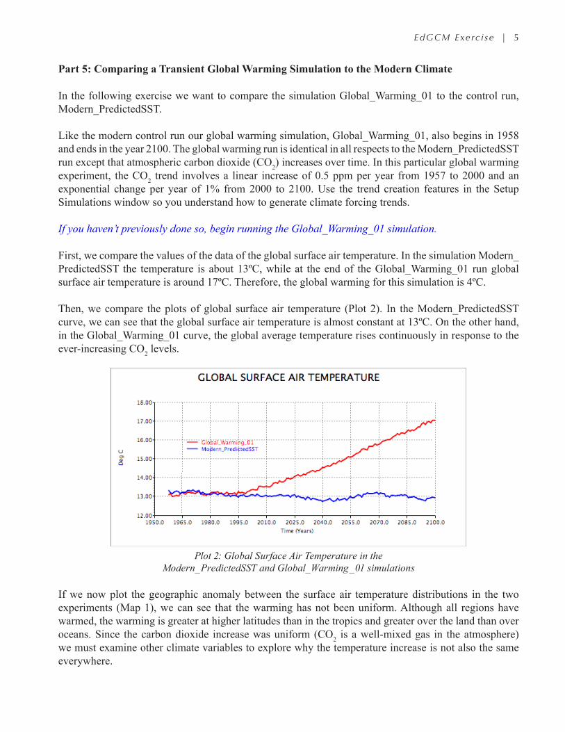
First, we compare the values of the data of the global surface air temperature. In the simulation Modern_PredictedSST the temperature is about 13ºC, while at the end of the Global_Warming_01 run global surface air temperature is around 17ºC. Therefore, the global warming for this simulation is 4ºC.

Then, we compare the plots of global surface air temperature (Plot 2). In the Modern_PredictedSST curve, we can see that the global surface air temperature is almost constant at 13ºC. On the other hand, in the Global_Warming_01 curve, the global average temperature rises continuously in response to the ever-increasing CO2 levels.

Plot 2: Global Surface Air Temperature in the Modern_PredictedSST and Global_Warming_01 simulations

If we now plot the geographic anomaly between the surface air temperature distributions in the two experiments (Map 1), we can see that the warming has not been uniform. Although all regions have warmed, the warming is greater at higher latitudes than in the tropics and greater over the land than over oceans. Since the carbon dioxide increase was uniform (CO2 is a well-mixed gas in the atmosphere) we must examine other climate variables to explore why the temperature increase is not also the same everywhere.

6 | E d GCM E x E r C i s E

Map 1: Annual Surface Air Temperature Anomaly

At this point you might ask students to do some “browsing” or work in an “exploration mode” to see if they can come up with hypotheses (supported by evidence) for why the planet warms in the way that it does.

One key element in the geographic distribution of warming is related to the ice-albedo feedback mechanism. This feedback is related to the fact that, as the climate warms, snow and ice begin to melt. As they do, the underlying surface reflects far less of the sun’s radiation than the highly-reflective snow and ice. The surface absorbs more energy and warms more than surrounding regions - further melting snow and ice cover.

Compare the areas of greatest snow decrease to the areas of greatest temperature increase (Map 2).

Are there other important feedbacks in the climate system that effect global warming?

Yes. Another important feedback relates to changes in cloud cover. In Map 3 below, we see that low clouds, which generally act to reflect sunlight and have a net cooling effect on the planet, will decrease as climate warms. As low cloud cover decreases, less sunlight is reflected back to space, and more of the sun’s energy is thus absorbed at the Earth’s surface, further heating the planet…a positive feedback to warming. It is interesting to note that if the cover of high clouds is also reduced, this could attenuate this feedback.

EdGCM Exerc i se | 7

Map 2: Annual Snow Cover Anomaly

Map 3: Annual Change in Low Cloud Cover

8 | E d GCM E x E r C i s E

Water Vapor:

Another reason for the overall warming is that increased evaporation from the oceans causes more water vapor to accumulate in the atmosphere. Water vapor is, itself, a powerful greenhouse gas, and thus it acts as a positive feedback, which further warms the climate. We can see that the increase in the global atmospheric water vapor content in the global warming simulation is nearly 30% from 1995 to 2100 (Plot 3).

Plot 3: Global Atmospheric Water Vapor Content in Modern_PredictedSST and Global_Warming_01 simulations.

HydrologicalCycle:MoistureBalance

As one might suspect, with more evaporation, and more water vapor in the atmosphere, global precipitation tends to increase. In Map 4, we can see that the average increase in the annual precipitation, due to the increase in the global temperature, is also not uniform, with greater increases in the tropics, where energy intensifies convection systems and at high latitudes where the now open oceans are a new source of atmospheric moisture that previously did not exist.

Unfortunately, what will eventually happen to water resources in a globally warmer world is a far more difficult task, since the ultimate fate of water resources will relate to the more complex balance between regional evaporation and precipitation rates. To exacerbate the problem of determining the impact of global warming on key hydrological variables, we expect that precipitation will tend to occur more and more in short-term, intense events (the hypothesis is that convective storms will increase due to more energy in the system). GCMs, with spatial resolutions coarser than typical thunderstorms, may not capture such phenomenon accurately enough to test such hypotheses….but you can try.

What conclusions would you draw from the climate model in EdGCM about the future of water resources on Earth in the 21st century?

EdGCM Exerc i se | 9

Map 4: Annual Precipitation Change

Map 5: Annual Change in Precipitation-Evaporation

10 | E d GCM E x E r C i s E

notes