Radar Target Tracking - ASU Digital Repository Target Tracking ... ABSTRACT As the demand for ......

Radar Target Tracking

with Varying Levels of Communications Interference

for Shared Spectrum Access

by

Jian Zhou

A Thesis Presented in Partial Fulfillmentof the Requirements for the Degree

Master of Science

Approved April 2015 by theGraduate Supervisory Committee:

Antonia Papandreou-Suppappola, ChairVisar Berisha

Narayan Kovvali

ARIZONA STATE UNIVERSITY

May 2015

ABSTRACT

As the demand for spectrum sharing between radar and communications systems

is steadily increasing, the coexistence between the two systems is a growing and very

challenging problem. Radar tracking in the presence of strong communications inter-

ference can result in low probability of detection even when sequential Monte Carlo

tracking methods such as the particle filter (PF) are used that better match the target

kinematic model. In particular, the tracking performance can fluctuate as the power

level of the communications interference can vary dynamically and unpredictably.

This work proposes to integrate the interacting multiple model (IMM) selection

approach with the PF tracker to allow for dynamic variations in the power spectral

density of the communications interference. The model switching allows for a neces-

sary transition between different communications interference power spectral density

(CI-PSD) values in order to reduce prediction errors. Simulations demonstrate the

high performance of the integrated approach with as many as six dynamic CI-PSD

value changes during the target track. For low signal-to-interference-plus-noise ratios,

the derivation for estimating the high power levels of the communications interfer-

ence is provided; the estimated power levels would be dynamically used in the IMM

when integrated with a track-before-detect filter that is better matched to low SINR

tracking applications.

i

ACKNOWLEDGEMENTS

I would like to give much thanks to my academic advisor, Dr. Antonia Papandreou-

Suppappola, to let me have the opportunity to work on researches with her. With all

her careful and detail-oriented guidance, I completed this work within the expected

time without any background stochastic signal processing knowledge before. I would

send special thanks to Antonia for her impressive patience in advising this research

projects and offer ideas concerning the tough obstacles. Her passion in signal pro-

cessing made me proud to be her student and her caring and positive life attitude has

given me a warm support living in a foreign country. It is a great honor and pleasure

to be her student and I will be grateful for her effective encouragement during all my

life.

I will also thank Dr. Visar Berisha and Dr. Narayan Kovvali for their willingness

to join in my graduate committee and take time to attend my thesis defense during

their heavy business, assisting and providing valuable advice to my thesis.

Special thanks go to my lab-mate, John Kota and Meng Zhou, for their effective

help and thoughtful ideas to me to better overcome the research difficulties. And

Thanks to all SPAS lab mates who have left me a unforgettable research experience.

Thanks to my parents, for bringing me up, with more than twenty years’ caring.

ii

TABLE OF CONTENTS

Page

LIST OF TABLES . . . . . . . . . . . . . . . . . . . . . . . . . . . . . . . . . . . . . . . . . . . . . . . . . . . . . . . . . v

LIST OF FIGURES . . . . . . . . . . . . . . . . . . . . . . . . . . . . . . . . . . . . . . . . . . . . . . . . . . . . . . . . vi

CHAPTER

1 INTRODUCTION . . . . . . . . . . . . . . . . . . . . . . . . . . . . . . . . . . . . . . . . . . . . . . . . . . . 1

1.1 Motivation . . . . . . . . . . . . . . . . . . . . . . . . . . . . . . . . . . . . . . . . . . . . . . . . . . . . . 1

1.2 Proposed Thesis Work . . . . . . . . . . . . . . . . . . . . . . . . . . . . . . . . . . . . . . . . . . 5

1.3 Thesis Organization . . . . . . . . . . . . . . . . . . . . . . . . . . . . . . . . . . . . . . . . . . . . . 6

2 TARGET TRACKING ALGORITHMS . . . . . . . . . . . . . . . . . . . . . . . . . . . . . . . 7

2.1 Nonlinear Tracking Models . . . . . . . . . . . . . . . . . . . . . . . . . . . . . . . . . . . . . . 7

2.2 Bayesian Estimations . . . . . . . . . . . . . . . . . . . . . . . . . . . . . . . . . . . . . . . . . . . 8

2.3 Sequential Importance Resampling Particle Filter . . . . . . . . . . . . . . . . . 9

2.4 Interacting Multiple Model . . . . . . . . . . . . . . . . . . . . . . . . . . . . . . . . . . . . . . 16

3 TARGET TRACKING IN VARYING INTERFERENCE POWER LEV-

ELS . . . . . . . . . . . . . . . . . . . . . . . . . . . . . . . . . . . . . . . . . . . . . . . . . . . . . . . . . . . . . . . . 19

3.1 Interacting Multiple Model with Sequential Importance Resampling

Particle Filter . . . . . . . . . . . . . . . . . . . . . . . . . . . . . . . . . . . . . . . . . . . . . . . . . . 19

3.2 Different Communications Interference Power Levels. . . . . . . . . . . . . . . 22

4 SIMULATIONS . . . . . . . . . . . . . . . . . . . . . . . . . . . . . . . . . . . . . . . . . . . . . . . . . . . . . 26

4.1 Low Environmental SINR for SIR-PF to Work . . . . . . . . . . . . . . . . . . . . 27

4.2 IMM with Varying Interference Power Level . . . . . . . . . . . . . . . . . . . . . . 30

4.3 IMM-PF Performances for Fixed-Gap Environmental SINR Pairs. . . 40

4.3.1 Gap Fixed at 10 dB . . . . . . . . . . . . . . . . . . . . . . . . . . . . . . . . . . . . . . 40

4.3.2 Gap Fixed at 4 dB . . . . . . . . . . . . . . . . . . . . . . . . . . . . . . . . . . . . . . . 43

iii

CHAPTER Page

4.4 IMM-PF Performance in Environments that Change in Different

Frequencies . . . . . . . . . . . . . . . . . . . . . . . . . . . . . . . . . . . . . . . . . . . . . . . . . . . . 45

4.5 Three Interference Power Levels . . . . . . . . . . . . . . . . . . . . . . . . . . . . . . . . . 48

4.6 Four Interference Power Levels . . . . . . . . . . . . . . . . . . . . . . . . . . . . . . . . . . . 52

5 EXTENSION TO ESTIMATING VARIANCE DYNAMICALLY . . . . . . . . 56

5.1 Scenario Settings . . . . . . . . . . . . . . . . . . . . . . . . . . . . . . . . . . . . . . . . . . . . . . . 56

5.2 GLRT and MLE Computation . . . . . . . . . . . . . . . . . . . . . . . . . . . . . . . . . . . 58

5.3 Detector and Performance . . . . . . . . . . . . . . . . . . . . . . . . . . . . . . . . . . . . . . . 61

5.3.1 Under Hypothesis H0 . . . . . . . . . . . . . . . . . . . . . . . . . . . . . . . . . . . . . 61

5.3.2 Under Hypothesis H1 . . . . . . . . . . . . . . . . . . . . . . . . . . . . . . . . . . . . . 62

5.4 Performance . . . . . . . . . . . . . . . . . . . . . . . . . . . . . . . . . . . . . . . . . . . . . . . . . . . . 63

5.5 Track-Before-Detect . . . . . . . . . . . . . . . . . . . . . . . . . . . . . . . . . . . . . . . . . . . . . 65

6 CONCLUSIONS AND FUTURE WORK . . . . . . . . . . . . . . . . . . . . . . . . . . . . . 66

6.1 Conclusions . . . . . . . . . . . . . . . . . . . . . . . . . . . . . . . . . . . . . . . . . . . . . . . . . . . . 66

6.2 Future Work . . . . . . . . . . . . . . . . . . . . . . . . . . . . . . . . . . . . . . . . . . . . . . . . . . . 67

REFERENCES . . . . . . . . . . . . . . . . . . . . . . . . . . . . . . . . . . . . . . . . . . . . . . . . . . . . . . . . . . . . 68

iv

LIST OF TABLES

Table Page

2.1 Resampling Algorithm . . . . . . . . . . . . . . . . . . . . . . . . . . . . . . . . . . . . . . . . . . . . . 15

2.2 Sequential Importance Resampling Particle Filter . . . . . . . . . . . . . . . . . . . . 16

2.3 Interacting Multiple Model Algorithm . . . . . . . . . . . . . . . . . . . . . . . . . . . . . . . 18

3.1 IMM Modes Transition through the Markov-chain Algorithm. . . . . . . . . . 21

3.2 Interacting Multiple Model Particle Filter Algorithm . . . . . . . . . . . . . . . . . 25

4.1 SINR Settings with Time for IMM Simulations . . . . . . . . . . . . . . . . . . . . . . . 31

4.2 SINR Values with Different Gaps Settings for IMM Simulations . . . . . . . 33

4.3 SINR Values Setting with IMM On and IMM Off . . . . . . . . . . . . . . . . . . . . 38

4.4 SINR Values with Fixed Gaps Settings for IMM Simulations . . . . . . . . . . 40

4.5 SINR Values with Fixed Gaps Settings for IMM Simulations . . . . . . . . . . 43

4.6 Environmental Conditions Changing Frequencies Settings . . . . . . . . . . . . . 46

4.7 SINR Values with Different Gaps Settings for IMM Simulations . . . . . . . 48

4.8 SINR Values Set in Four Interference Power Levels . . . . . . . . . . . . . . . . . . . 52

4.9 SINR Setting with Time . . . . . . . . . . . . . . . . . . . . . . . . . . . . . . . . . . . . . . . . . . . . 52

v

LIST OF FIGURES

Figure Page

4.1 RMSE of Position for SINR Ranging from 1 dB to 11 dB in Log Scale . 28

4.2 RMSE of Position for SINR Ranging from 5 dB to 15 dB in Log Scale . 29

4.3 RMSE of Position for SINR Ranging from 17 dB to 27 dB in Log Scale 29

4.4 Ideal IMM Mode Probability with Time . . . . . . . . . . . . . . . . . . . . . . . . . . . . . 32

4.5 The RMSE of SINR Gaps Ranging from 2 dB to 12 dB in Log Scale . . . 33

4.6 The RMSE of SINR Gaps Ranging from 2 dB to 12 dB . . . . . . . . . . . . . . . 34

4.7 The RMSE of SINR Gaps Ranging from 14 dB to 24 dB in Log Scale . . 34

4.8 The RMSE of SINR Gaps Ranging from 14 dB to 24 dB . . . . . . . . . . . . . . 35

4.9 Probabilities for SINR Gaps Ranging from 2 dB to 12 dB . . . . . . . . . . . . . 36

4.10 Probabilities for SINR Gaps Ranging from 14 dB to 24 dB . . . . . . . . . . . . 37

4.11 Performances Between IMM On and IMM Off. . . . . . . . . . . . . . . . . . . . . . . . 39

4.12 The RMSE of the SINRs with Fixed Gap in Log Scale . . . . . . . . . . . . . . . . 41

4.13 The RMSE of the SINRs with Fixed Gap . . . . . . . . . . . . . . . . . . . . . . . . . . . . 41

4.14 The Mode Probabilities of SINRs with Fixed Gap . . . . . . . . . . . . . . . . . . . . 42

4.15 Performance for SINR Difference Fixed at 4 dB . . . . . . . . . . . . . . . . . . . . . . 44

4.16 IMM Performance for SINR Difference Fixed at 4 dB . . . . . . . . . . . . . . . . . 45

4.17 IMM Performance with Environmental Conditions Changes in Differ-

ent Frequencies . . . . . . . . . . . . . . . . . . . . . . . . . . . . . . . . . . . . . . . . . . . . . . . . . . . . 47

4.18 The RMSE of the SINRs with Gap from 2 dB to 12 dB in Log Scale . . . 49

4.19 The RMSE of the SINRs with Gap from 2 dB to 12 dB . . . . . . . . . . . . . . . 50

4.20 The Mode Probabilities of SINRs from 2 dB to 12 dB . . . . . . . . . . . . . . . . 51

4.21 The Mode Probabilities of Four Interference Power Levels . . . . . . . . . . . . . 53

4.22 The RMSE of Four Interference Power Levels in Log Scale . . . . . . . . . . . . 54

4.23 The RMSE of Four Interference Power Levels . . . . . . . . . . . . . . . . . . . . . . . . 55

vi

Chapter 1

INTRODUCTION

1.1 Motivation

One of the main functions of modern radars is target tracking, both for military

and civil applications. For military applications, radars are used to detect and track

enemy combatants, whereas in civil applications, modern radars help in navigation

and collision avoidance in the aviation field [1]. The basic working principle of radars

is to transmit a particular type of waveform and then observe the returned signal in

order to detect the existence of a target. By processing the differences between the

transmitted and the returned signals, we can acquire the position and velocity of the

target by estimating the time delay and the Doppler shift parameters. The target’s

position can be determined by the time delay whereas the velocity of the target can

be determined by the Doppler shift. The time delay and Doppler shift parameters

form the state parameter at a given time step [2]. The radar tracking problem’s

main task is to dynamically estimate sequentially the state of the target given noisy

measurements [3].

Radar’s most fundamental function is to detect the existence of a target and then

to track its movement. These detection and tracking processes require radar systems

to process all received measurements. However, the noise power of the environment

can affect the accuracy of detection and tracking. Different methods have been devel-

oped based on the type of noise and signal-to-noise ratio (SNR) level. In analyzing

the detection accuracy, two significant parameters that reflect the detection perfor-

mance are the probability of detection PD and the the probability of false alarm PFA.

1

Using the Neyman Pearson thereon test statistic, the PFA can be fixed to a desirable

level to provide a threshold for the PD [4, 5].

Different methods have been developed to perform radar tracking, following the

problem’s state space formulation. In dealing with the analysis and estimation of

dynamic systems, the Bayesian approach, which provides a rigorous general frame-

work for dynamic state estimation problems, is suited for the probabilistic state-space

formulation. Following the Bayesian approach to dynamic state estimation, the pos-

terior probability density function (PDF) of the state is estimated using all available

measurements, from the initial time step to the current time step. Different asso-

ciation algorithms have been developed to relate the measurements to the tracking

system’s estimated states using likelihood functions. Different types of optimal and

sub-optimal algorithms to implement Bayesian approach have also been considered

[6, 7].

One of the most commonly used state-space optimal Bayesian estimators is the

Kalman filter [8, 9]. The Kalman filter implements the minimum-variance state esti-

mator for linear dynamic systems with Gaussian noise by assuming that the PDF at

every time step is Gaussian. The Gaussian characteristic simply requires to represent

the PDF using only two parameters: mean and covariance [10]. The filter works re-

cursively to estimate both the targets’ states as well as the uncertainty covariance of

the estimated states. The estimated state is implemented using a state transitional

model from the posterior PDF from the previous time step. The filter then updates

the estimated states using the received measurements to obtainthe posterior PDF. Al-

though the Kalman filter is often used, many systems are nonlinear and are modeled

using non-Gaussian processes. For such systems, sub-optimal estimation algorithms

have been developed. The extended Kalman filter (EKF) is obtained by applying

the first-order partial derivative to linearize the transition or measurement models

2

[11, 12]. This step approximately linearizes a nonlinear system so that it can be used

with a Kalman filter. The EKF has provided a good solution to state estimations of

nonlinear dynamic systems. However, as it only provides first order approximation

terms, it can introduce large errors when compared to the true posterior PDF. The

unscented Kalman filter (UKF) has been developed as another nonlinear-adapting

modification to the Kalman filter [13]. The UKF estimates the mean and covariance

by using the unscented transform to approximate the first three moments of the pos-

terior PDF using a set of samples. Without involving any linearization steps, the

UKF has been shown to perform better than the EKF as discussed in [14].

Another sub-optimal Bayesian estimation filter adapted to nonlinear and non-

Gaussian systems is the particle filter (PF). The particle filter is a sequential Monte

Carlo method that approximates the posterior PDF using a finite set of particles

and corresponding weights. The weight determines the importance of a particle in

estimating the targets’ states. After evolving with every time step, the weights are

updated by the likelihood function that relate the measurements with the estimated

states. The choice of the importance function determines the performance of PF [15].

By adopting the particle filter, the tracking system can be solved under nonlinear and

non-Gaussian conditions.

The tracking problem becomes more challenging when the target is sharing the

spectrum with communications signals as this results in a low signal-to-interference-

plus-noise ratio (SINR) operating point for the radar receiver. Of particular concern is

the problem of radar and communications coexistence in the S band, where the com-

munications interference is due to long term evolution (LTE) time division duplexing

(TDD).

The standard of LTE is established and presented by the 3rd generation part-

nership project (3GPP) as an upgrade to the Universal Mobile Telecommunications

3

System (UMTS) [16]. When compared to previous generations of communication

technologies, LTE exhibits higher user data rates, larger system capacities, less delays,

and improved spectral efficiencies [17]. Based on former modular system structures of

3GPP, LTE mainly adopts orthogonal frequency division multiple access (OFDMA)

as for downlink data transmission, and single-carrier frequency division multiple ac-

cess (SC-FDMA) for uplink data transmission. According to the different duplex

model, LTE can be divided into LTE time division duplex (LTE-TDD) and LTE

frequency division duplex (LTE-FDD). The working frequencies for LTE-TDD is 3.5

GHz according to the spectrum allocation work of FCC. This technology has been

applied in applications including public security, situational awareness, monitoring

and interventional applications, machine-to-machine communications, and military

communications.

OFDMA is an extension of OFDM that makes OFDM available for multi-user

applications. In OFDMA, different sub-channels can be allocated to different users.

In order to identify the sub-channel of a specific user, adjacent sub-channels are

usually allocated to the same user to simplify the process. This extension enables

different users to transmit and receive data simultaneously, so that multiple users

can benefit from the use of OFDM [17]. On the other hand, different sub-frames

are allocated for different functions, including downlink, uplink, guard, or pilot. As

different signals are used for different functions, different time frames of LTE are

expected to have different power levels.

This dynamically varying communications signal power characteristic of LTE-

TDD further complicates radar tracking as it results in a dynamically varying SINR

for the tracker at the radar receiver. When a PF is used for tracking, changes in

SINR can result in inaccuracies in the likelihood function computation as the particles

weights will be updated by inaccurate measurement information.

4

To solve the noise-varying problem, various studies have been published to improve

the optimal and sub-optimal Bayesian estimation algorithms. In [18], a probability

hypothesis density filter, implemented using a PF, is presented to dynamically esti-

mate the power levels of the measurement noise as well as the state parameters of

multiple targets. In [19], a modification to the PF is developed to deal with correlated

noise for both the states propagation model and the measurements model. In [20], a

sequential importance sampling Bayesian estimation approach with marginalization

is used to estimate the target states as well as the parameters of additive Gaussian

noise.

1.2 Proposed Thesis Work

In this work, we propose to solve the coexistence of radar and communications

problem in the presence of dynamically varying power levels of communications in-

terference for radar tracking using the interacting multiple model (IMM) approach.

In particular, we integrate the radar tracker at the receiver with the ability to switch

between different plausible interference power levels in order to reduce the overall

tracking error.

The main feature of the IMM algorithm is that it provides the ability to dynam-

ically switch between several possible model modes when estimating the state of a

dynamic system [21, 22]. Different target tracking studies have used the IMM to

account for different possible states propagation models. In [23], the IMM was used

to track a highly maneuvering target using three different kinetic models. In [24],

the IMM estimator was used to implement an algorithm to handle a transition prob-

ability matrix with variable measurements sampling intervals. In [25], the IMM was

integrated with the UKF to track maneuvering targets in air traffic control (ATC)

applications.

5

Our proposed IMM-based algorithm assumes several possible power levels of com-

munications interference and a fixed power level of environmental noise. A mode

variable, representing filter settings for different power levels of communication inter-

ference, are assigned to every particle of the PF tracker. The corresponding particle

weight is updated using the likelihood function determined by the selected mode.

By applying the recursion of the PF, the probability of a particular mode among all

the particles changes based on the interference power level, resulting in an overall

improvement in tracking performance. Simulations are presented to show the perfor-

mance of the proposed algorithm.

As the actual interference power levels are not known a priori in realistic scenarios,

we also consider an approach for estimating the interference power level for medium to

high SINR values. We formulate the problem as a detection hypothesis and derive the

detection statistic using a generalized likelihood ratio test (GLRT). Using the GLRT,

we compute the maximum likelihood estimates of the interference power level, as well

as range and range-rate. This work can be integrated with the proposed IMM-based

algorithm by dynamically estimating the interference power level at each time step

and using the estimated value into the PF or a track-before-detect filter (TBDF)

[26, 27, 28, 29] to obtain improved estimates of the target parameters.

1.3 Thesis Organization

This thesis is organized as followed. In Chapter 2, we review the particle filter

tracker and the interacting multiple model approach. In Chapter 3, we propose the

PF tracking with the integrated IMM with varying power levels of communications

interference, and we provide simulations examples in Chapter 4. In Chapter 5, we

present a method that estimates the communications interference power level dynam-

ically. Conclusion and future work are discussed in Chapter 6.

6

Chapter 2

TARGET TRACKING ALGORITHMS

2.1 Nonlinear Tracking Models

For tracking problems represented by a dynamic state-space model, the state

transition model is given by [15]:

xk = f(xk−1) + vk−1 (2.1)

where k represents the time step, xk is the state vector describing the position and

velocity of the moving target, f(·) is the state transition function, and vk is a random

process used to model the state propagation modeling error.

The measurement equation model is given by a possibly nonlinear function that

describes the physical relationship of the state xk with the measurement zk:

zk = h(xk) + uk (2.2)

where zk is the measurement vector and uk is the observation noise vector at time

step k. In radar target tracking applications, the radar receiver must first determine

whether the signal received consists of simply noise or the noisy transmitted signal

after it has been reflected off a moving target. If a target reflection is detected,

then the receiver must recursively estimate the unknown state of the target given

the noisy measurements. From the Bayesian perspective, the problem translates to

estimating the posterior probability density function (PDF) p(xk|z1:k), where z1:k =

{z1, z2, . . . , zk} is the set of all measurements up to time k.

7

2.2 Bayesian Estimations

Bayesian’s theorem [30], which relates the posterior PDF to the current measure-

ments, can be used to provide a solution to the state-space formulation problem. In

particular, a solution can be obtained by recursively computing the state estimate

in the Bayesian sense by iteratively computing the posterior PDF using a two-step

process: predicting the state and updating the state using the measurements.

The estimation step involves the prediction of the target state at time step k based

on the posterior PDF p(xk−1|z1:k−1) at time step k − 1, using the state propagation

model in Equation (2.2). Using the Chapman-Kolmogorov equation, stated in [31],

we can compute a prediction of the state by evaluating

p(xk|z1:k−1) =

∫p(xk|xk−1)p(xk−1|z1:k−1)dxk−1 (2.3)

where p(xk|xk−1) represents the transition model in Equation (2.1). Since state xk−1

was obtained using all measurements up to time step k−1, the following relationships

hold

p(xk|xk−1) = p(xk|xk−1, z1:k−1) (2.4)

p(xk−1|z1:k−1) = p(xk−1|zk−1)

p(xk|z1:k−1) = p(xk|zk−1)

Using the relationships in Equation (2.4), we can modify Equation (2.3) to

p(xk|zk−1) =

∫p(xk|xk−1)p(xk−1|zk−1)dxk−1 (2.5)

Up to this point, only measurements up to the previous time step have been used to

predict the state. As a result, some estimation errors are expected when comparing

the true and estimated tracks. In order to improve the accuracy of the tracking, we

8

need to update the estimate using the measurement at the current time step k. The

resulting update on the posterior PDF is given by

p(xk|zk) =p(zk|xk)p(xk|zk−1)

p(zk|zk−1)(2.6)

where p(zk|xk) is the likelihood PDF from Equation (2.2), representing the relation-

ship between the measurements and the target states information and p(xk|zk−1) de-

notes the prior PDF acquired from the estimation step. If the measurement function

h(·) does not vary with time, p(zk|zk−1) is the normalizing constant:

p(zk|zk−1) =

∫p(zk|xk)p(xk|zk−1)dxk (2.7)

After the prediction and update steps, as time evolves, the states information xk is

determined by the updated posterior PDF, acquired at each time step. Thus, the

prediction and update steps provide the basis for the tracking problem. However, the

details on these steps, such as determining the posterior and prior PDFs, are required

to be determined analytically according to different applications. In this thesis work,

we use the sequential importance resampling particle filter to recursively compute the

prediction and update steps.

2.3 Sequential Importance Resampling Particle Filter

In target tracking problems, the system is modeled by the state propagation model

in Equation (2.1) which can consist of both constant and dynamically varying state

parameters. All of these methods work to filter the state, formed by a Markov chain

time transition, from measurements that are degraded by noise as well as some other

forms of random perturbations. The Markovian characteristics of the evolving system

have kept the distribution of the states at the current time independent of the states

at the previous steps [32].

9

Some Bayesian filtering solutions include the Kalman filter (KF) [33], extended

Kalman filter (EKF) [34, 35], unscented Kalman filter (UKF) [14], and particle filter

(PF). The KF assumes that both the state propagation model in Equation (2.1) and

the measurement model in Equation (2.2) are linear. Also both the modeling error

random process and the measurement noise are assumed to be Gaussian so that the

states can be simply described by their means and covariances [33]. However, since

not all models and random processes in actual applications are linear and Gaussian,

the EKF and UKF have been used as alternatives to the KF. For EKF, a first-order

Taylor series expansion is used to linearize the state propagation model function.

Once the filter uses linearized functions as propagation functions then it can proceed

using the steps of a KF [34, 36, 37]. For UKF, instead of computing and evolving

the Jacobian matrices, the unscented transform is used to represent the Gaussian

random variable of the states with a set of deterministically chosen samples that

capture the first two moments of the Gaussian distribution [32]. These set of finite

samples are propagated through the state propagation model and then updated by

the measurements. The final estimate is made based on these processed samples.

The particle filter is another way to solve Bayesian estimation problems. It is

a sequential Monte Carlo approach known as bootstrap filtering [38]. Compared to

KF, EKF, and UKF, particle filters are available for both non-Gaussian processes

and nonlinear state propagation and measurement models. Using a particle filter,

the posterior PDF is represented by a finite set of discrete and independent particles

along with their weights. The particles are working as the system states’ Monte

Carlo samples. Just like other Monte Carlo approaches, the result will become more

accurate as the number of samples increases.

10

The particle filter starts from the idea of sequential Monte Carlo estimation based

on particles representing a PDF. For a multidimensional integral:

I =

∫g(x)dx (2.8)

the Monte Carlo method provides a factorization to the integral into the product of

another variable f(·) and a probability density π(·):

I =

∫f(x)π(x)dx (2.9)

with the restriction that π(x) > 0 and∫π(x)dx = 1.

To use it in the state model, the states xk and the posterior PDF can be repre-

sented in terms of particles and their corresponding weights. The particles used in

this filter come from importance sampling [15, 38]. Specifically,

{x(n)k , w

(n)k }

Npn=1 (2.10)

represents particles x(n)k and corresponding weights w

(n)k , n = 1, . . ., Np.

All weights are normalized:Np∑n=1

w(n)k = 1 (2.11)

The posterior PDF can be represented as

p(xk|zk) ≈Np∑n=1

w(n)k δ(xk − x

(n)k ) (2.12)

where δ(x) is the Dirac delta function, which is non-zero only when x = 0. This

equation describes how the posterior PDF is represented by particles and their cor-

responding weights in the particle filter. The approximation will become equal if the

particle numberNp is asymptotically large. Each independent particle will be assigned

with its only weight. The final estimate xk is calculated by the linear combination of

all particles states, weighted by the corresponding weights,

xk =

∫xkp(xk|zk)dxk =

Np∑n=1

w(n)k x

(n)k (2.13)

11

According to the importance sampling, the weights are drawn from the ratio between

the probability density π(·) and the proposed importance density q(·)

w(n)k ∝

π(x(n)k )

q(x(n)k )

(2.14)

For the prior PDF case, the above equation can be expanded as

w(n)k ∝

π(x(n)k |zk)

q(x(n)k |zk)

(2.15)

In the sequential importance sampling case, according to Bayesian estimation update

step, we can represent p(x(n)k |zk) as

p(x(n)k |zk) =

p(zk|xk)p(xk|zk−1)p(zk|zk−1)

(2.16)

p(zk|xk)p(xk|zk−1)p(zk|zk−1)

=p(zk|xk)p(xk|xk−1)

p(zk|zk−1)p(xk−1|zk−1) (2.17)

When the measurement model and p(zk|zk−1) do not vary with time. Equation (2.16)

and Equation (2.17) can be combined to form

p(x(n)k |zk) ∝ p(zk|xk)p(xk|xk−1)p(xk−1|zk−1) (2.18)

In order to propagate the weights at every time step, the importance density function

needs to be chosen such that it satisfies the property of factorization

q(xk|zk) = q(xk|xk−1,xk)q(xk−1|zk−1) (2.19)

By substituting Equation (2.19) and Equation (2.18) into Equation (2.15), the weights

updating expression from time step k − 1 to k becomes

w(n)k ∝

p(zk|xk)p(xk|xk−1)p(xk−1|zk−1)q(xk|xk−1, zk)q(xk−1|zk−1)

w(n)k ∝ w

(n)k−1

p(zk|xk)p(xk|xk−1)q(xk|xk−1, zk)

(2.20)

12

The choosing of the importance function will affect the performance and computa-

tional cost of the filter. Proposed methods like local linearization techniques are usu-

ally taken to construct suboptimal approximation of the optimal importance density,

by taking a Gaussian approximation of the posterior PDF p(xk|zk) [15, 39]. However,

researchers often just choose the prior probability distribution to be the importance

density function

q(xk|xk−1, zk) = p(xk|xk−1) (2.21)

This simplifies the weight update equation. Using Equations (2.20) and (2.21), the

weight update step is simplified as multiplying the particle weight from the last time

step with the likelihood function

w(n)k ∝ w

(n)k−1p(zk|xk) (2.22)

The simplified weights update step has made it possible for the algorithm to be

implemented with higher efficiency but less computational costs.

With the particle states propagating recursively and then updated by the measure-

ments received at each time step, the sequential importance sampling (SIS) particle

filter works to approximate the true posterior PDF p(xk|zk). A prominent problem

for the SIS particle filter is the degeneracy problem. Firstly, all particles are assigned

with equal weights. However, after a few iterations, significant weights are shared by

only a few particles and a large amount of particles will have no contribution to the

approximation of the posterior PDF. This problem causes an extreme waste on com-

putational cost by updating particles with negligible weights. Also the degeneracy

makes the SIS filtering loose its advantages by using Monte Carlo methods [32, 39].

To solve the problem and make the algorithm consistent, resampling has been used

to solve the degeneracy problem.

13

The main idea for the resampling is to duplicate the particles with significant

weights. After resampling, particles with little weights will be pruned, and particles

with large weights will be duplicated. At the first step of the resampling, a cumulative

weight will be generated for all particles. Then, a metric is used on the weight particles

to decide whether the particle should be pruned. This step starts with drawing a

positive random number smaller than the average weight, as the metric for the first

iteration. For each iteration, the metric is calculated by adding the average weight to

the metric of last iteration cumulatively. If the cumulative weight value is larger than

the metric, the particle will be kept. Meanwhile, the pruned particle will be replaced

by the particle duplicated from the last iteration. The particles will keep being pruned

until the cumulative weights value is larger than the metric. The algorithm will be

concluded in Table 2.1.

14

Table 2.1: Resampling Algorithm

{x(j)k , w

(j)k }

Npj=1 = RESAMPLE[{x(i)

k , w(i)k }

Npi=1]

� Initialize the cumulative weight: c1 = w(1)k

� For i = 2 : Np

- Construct the cumulative weight: ci = ci−1 + w(i)k

� End For

� Start at the beginning of the metric: i = 1

� Draw a starting point that is uniform between 0 and 1/Np: u1 ∼ U [0, 1/Np]

� For j = 1 : Np

- Move along the metric: uj = u1 + 1/Np(j − 1)

- While uj > ci

- Set i = i+ 1

- End While

- Assign sample: x(j)k = x

(i)k

- Assign weight: w(j)k = 1/Np

� End For

After the resampling, the particles will be assigned with equal weights. The target

states at this time step can be estimated by the linear combination of the new set of

particles with their equal weights. This process eliminates the degeneracy problem

as time evolves. On the other hand, the resampling process solved the computational

complexity problem of the SIS particle filter, thus increasing the tracking performance

of the filter.

To illustrate clearly the algorithm of Sequential Importance Resampling (SIR), a

table of pseudo is presented in Table 2.2.

15

Table 2.2: Sequential Importance Resampling Particle Filter

{x(j)k , w

(j)k }

Npj=1 = SIR[{x(i)

k−1, w(i)k−1}

Npi=1, zk]

� For i = 1 : Np

- Draw x(i)k ∼ p(xk|x(i)

k−1)

- Calculate w(i)k = p(zk|x(i)

k )

� End For

� Calculate Total Weight: t =∑Np

i=1 w(i)k

� For i = 1 : Np

- Normalize: w(i)k = w

(i)k /t

� End For

� {x(j)k , w

(j)k }

Npj=1 = RESAMPLE[{x(i)

k , w(i)k }

Npi=1]

2.4 Interacting Multiple Model

As for some state-space formation models, there exist the requirements for the

system to manage multiple models. In the problem in this thesis, as the interference

power levels are dynamically changing, the measuring model is also changing, thus

the target tracking system must select the correct measurement model to use at each

time step. To satisfy this demand, the interacting multiple model (IMM) is a solution

to this problem.

The state-space model for IMM is shown in the following equations:

xk = f(xk−1) + vk−1 (2.23)

zk = hk,mk(xk) + uk,mk (2.24)

where mk is the correct model to be selected at time step k. We define the selected

16

model as the filter mode. The mode variable mk is a finite state Markov Chain taking

values in {1, 2, . . . ,M} according to a transitional probability matrix B [21].

To manage different modes, we give each mode of the filter a probability µmk . The

sum of all mode probabilities should be 1. The final estimation provided by the filter

will be the linear combination of all filter modes weighted by its probabilities

M∑mk=1

µmk = 1

xk =M∑

mk=1

xk,mkµmk

To better note the probabilities in different steps in IMM, we represent the prior

probability as µmk|mk−1, and the posterior probability as µmk|mk . The prior mode

probabilities are acquired from the mixing step, calculated by the mode transition

probability matrix B. The posterior mode probabilities are updated by the likelihood

function of the corresponding filter mode.

At the beginning of every iteration, all mode probabilities will be updated by the

mixing step:

µmk=j|mk−1=∑i

[B]ijµmk−1=i|mk−1(2.25)

where [B]ij is the ijth element of matrix B.

Then, all mode states will be updated through Bayesian filtering based on the

measurement data, as Equation (2.6):

p(xk,mk |zk;mk) =p(zk|xk;mk)p(xk|zk−1;mk)

p(zk|zk−1;mk)(2.26)

where p(zk|xk;mk) represents the likelihood function for mode mk, and p(xk|zk−1;mk)

representing the filter’s prior estimation using Equation (2.23).

After the update of the states, the probabilities µmk|mk−1will be updated using

µmk|mk =µmk|mk−1

p(zk|xk;mk)∑mkµmk|mk−1

p(zk|xk;mk)(2.27)

17

After the updating of both the states xk for each mode and the corresponding mode

probability, the final state estimate is given by

xk =M∑

mk=1

xk,mkµmk|mk (2.28)

The posterior PDF p(xk,mk |zk;mk) for each mode mk, and the corresponding mode

probabilities µmk|mk will be propagated to the next time step.

The IMM algorithm steps are summarized in Table 2.3.

Table 2.3: Interacting Multiple Model Algorithm

[p(xk|zk,mk), µmk|mk ] = IMM[p(xk−1|zk−1,mk−1), µmk−1|mk−1]

� Mixing/Interacting: µmk=j|mk−1=∑

i[B]ijµmk−1=i|mk−1

� For mk = 1:M

- Predict and update steps: p(xk−1|zk−1;mk)→ p(xk|zk;mk)

- Update probabilities: µmk|mk−1→ µmk|mk

� End For

� Final Estimation: xk =∑M

mk=1 xk,mkµmk|mk

18

Chapter 3

TARGET TRACKING IN VARYING INTERFERENCE POWER LEVELS

3.1 Interacting Multiple Model with Sequential Importance Resampling Particle

Filter

For tracking problems, targets are possible to have different modes of moving.

To achieve better tracking accuracy, the tracking system needs to have the ability

of selecting from different state propagation models [40, 41]. This has been imple-

mented as an application of interacting multiple model (IMM) in multi-path tracking

problems. In this thesis, as different sub-frames of long term evolution with time

division duplex (LTE-TDD) are using different modulation schemes, the difference

in modulating signal makes the signals differed in power levels. Several variance lev-

els of measurement noise, due to different communications interference power levels

as the environmental signal-to-interference-plus-noise ratio (SINR) changes, are as-

sumed to be known by the tracking system. All the possible modes will be considered

in a discrete-valued vector. Different from the continuous-valued vectors, like target

kinematic variables including positions and velocities, discrete-valued vectors can be

referred to as Markov jump process. The algorithm proposed in this chapter is the

combination of the sequential importance resampling particle filter (SIR-PF) and the

IMM. This proposed algorithm has the ability to perform nonlinear filtering with

switching dynamic models, thus providing a solution to the interference power levels

varying problem [7, 42, 43].

To better specify the problem for the discrete-valued modes, an independent vari-

able representing system modes is added together with the target states. The system

19

with both continuous-valued target states and discrete-valued mode variables can be

described as

xk = f(xk−1) + vk−1 (3.1)

zk = hmk(xk) + ik,mk + uk,mk (3.2)

where mk is the mode at the time step k, and ik,mk is the interference at time step k

with power level prescribed by mode mk. Equation (3.1) represents the state prop-

agation model and Equation (3.2) represents the corresponding measurement model

with mode mk.

The particle will be represented in terms of both the targets’ states x(n)k , the filter

mode m(n)k , and the corresponding weight w

(n)k

{x(n)k ,m

(n)k , w

(n)k }

Npn=1 (3.3)

At the beginning of each iteration, different from the mixing step in the ordinary

IMM, the mode of every particle is transitioned through the finite-state Markov-

chain model. The probability matrix for mode transition (using a two-mode case as

an example) is denoted as π

π =

πii πij

πji πjj

(3.4)

where πii and πjj denotes the probability that the particle will keep its mode, πij

denotes probability that the particle’s mode will switch form mode i to mode j, and

πji denotes probability that the particle’s mode will switch form mode j to mode i.

The process can be extended to cases with more modes. The mode transition step is

shown below:

m(n)k = g(m

(n)k−1) (3.5)

where g(·) represents the mode transition process.

20

The algorithm of the particles’ modes transition is summarized in the Table 3.1.

Table 3.1: IMM Modes Transition through the Markov-chain Algorithm

[mk] = MODE-TRANSITION g(mk−1)

� For n = 1 : Np

- Draw u ∼ U [0, 1]

- If m(n)k−1 = i & u <= πii

· mk = i

- Else if m(n)k−1 = i & πii < u <= πii + πij

· mk = j

- Else if m(n)k−1 = j & u <= πjj

· mk = j

- Else if m(n)k−1 = j & πjj < u <= πjj + πji

· mk = i

� End for

After the modes’ transition, the target states of each particle is propagated using

Equation 3.1

x(n)k = f(x

(n)k−1) + vk−1 (3.6)

The weights’ update step is the same as for the SIR-PF, except that each particle

will choose likelihood function according to its mode

zk = h(xk) + ik,mk + uk

w(n)k = w

(n)k−1p(zk|x

(n)k ;mk) (3.7)

After the resampling, only particles with large weights survive. Since the values of

the weights are determined by the likelihood functions p(zk|x(n)k ;mk) , particles with

21

modes that match the environmental conditions will have larger weights and will

survive. The resampled particles as well as the particles’ weights and modes will be

propagated to the next time step.

The final estimation of IMM-PF is the same as SIR-PF:

xk =

Np∑n=1

w(n)k x

(n)k

At the beginning of the next time iteration, the mode for each particle is transited

through the Markov-chain process. The switching between different modes will be

determined by the mode transition probability matrix π. If the environmental con-

ditions changes at this time step, these “small amount of particles” that have the

same mode with the environment will be retained and duplicated. The transition

of particle modes through the Markov-chain process actually provides the ability for

IMM to select the right mode for the filter. The particle transition algorithm for two

modes is provided in Table 3.1 as an example. Cases with number of modes greater

than two can be extended easily from this algorithm.

Next, we discuss the use of the IMM when the power levels of the communications

interference varies over the track duration.

3.2 Different Communications Interference Power Levels

As we have discussed in the last section, the state propagation model stays the

same as Equation (3.8). In the measurement model in Equation (3.11), the variance

of the independent and identically distributed communications interference samples

in vector ik,mk that is added to the measurement in Equation (3.2), will vary with

time. As described above, the IMM-PF is used in high SINR environments, where

22

the possible variances of communications interference and noise are supposed to be

known. The filter is able to select the right mode according to the environmental

conditions.

xk = Fxk−1 + vk−1 (3.8)

where xk is the target state including the positions and the velocities in 2-D Cartesian

coordinate

xk =

xk

yk

xk

yk

(3.9)

where xk and yk are the target positions in 2-D coordinates and xk and yk are the

corresponding velocities. F is the state transition model matrix for the linear model:

F =

1 0 ∆T 0

0 1 0 ∆T

0 0 1 0

0 0 0 1

(3.10)

where ∆T is the time interval between two consecutive time steps. The value of ∆T

is determined by the sampling frequency. The term vk is the random process with

covariance matrix Q used to model the transition modeling error:

vk ∼N (0, Q)

The following equation is the measurement model for the target tracking in interfer-

ence variance varying environments:

zk = h(xk) + ik,mk + uk (3.11)

23

where zk represents the noisy measurement data, and h(·) is the measurement model

transformation function, relating the measurement term with the target state:

h(xk) =

r

r

=

√x2k + y2k

xk·xk+yk·yk√x2k+y

2k

(3.12)

In the measurement model, ik,mk represents the communications interference, which

we assumed to be wide-sense-stationary (WSS) Gaussian process in this thesis, and

uk is the environmental additive white Gaussian noise.

The transition of the mode is determined by the Markov jump process, like we

have described above. As time evolves, system modes will jump between possible

modes in the deterministic probabilities. The transitional probabilities can be set as:

πii = (mk = i|mk−1 = i) i = 1, 2, ... (3.13)

πij = (mk = j|mk−1 = i) i, j = 1, 2, ... and j 6= i (3.14)

The transition matrix is given as in Equation 3.4, for the two mode case.

However, the tracking result can be affected by the threshold that was set in the

Markovian transition process. The Markovian process propagation algorithm is the

same as the one in Table 3.1.

The difference for each mode is located at the weight update step. In the SIR-PF,

the weights are updated using the likelihood function. Compared to the normal SIR-

PF, the proposed algorithm updates each particle’s weight using the specific mode of

likelihood function according to the particle’s mode m(n)k . The weights are computed

in the following:

w(n)k = w

(n)k−1p(zk|x

(n)k ;mk) (3.15)

where p(zk|x(n)k ,mk) represents likelihood function for different modes. Since different

power levels of communications interference will have different variances, likelihood

functions of different modes will differ in the variance’s values.

24

Then, the particles with newly attributed weights will be resampled. During this

process, particles with mode different from the environmental conditions are pruned.

And those with the same mode and also close target state estimates will be duplicated

and then propagated to the next step. Finally the system selects the right mode for

the filter.

After the resampling, the tracked state is given by

xk =

Np∑n=1

w(n)k x

(n)k (3.16)

The algorithm of the IMM-PF is summarized in Table 3.2.

Table 3.2: Interacting Multiple Model Particle Filter Algorithm

{x(s)k ,m

(s)k , w

(s)k }

Nps=1 = IMM-PF[{x(n)

k−1,m(n)k−1, w

(n)k−1}

Npn=1, zk]

� For n = 1 : Np

- Propagate m(n)k = g(m

(n)k−1)

- Draw x(n)k ∼ p(xk|x(n)

k−1)

- Calculate w(n)k = p(zk|x(n)

k ;m(n)k )

� End for

� Calculate Total Weight: t =∑Np

n=1w(n)k

� For n = 1 : Np

- Normalize: w(n)k = w

(n)k /t

� End for

{x(s)k , w

(s)k ,m

(s)k }

Nps=1 = RESAMPLE[{x(n)

k , w(n)k ,m

(n)k }

Npn=1]

Compared to the SIR-PF algorithm in Table 2.2, the IMM-PF algorithm intro-

duced the mode transition for each particle before the weights calculation and the

weights are calculated using different likelihood functions according to their mode.

Also, the mode state for each particle will be processed in the resampling process.

25

Chapter 4

SIMULATIONS

To simulate the signal added with communication interference and noise, we sup-

pose that the noise and interference were directly added on the observed real states

without using the linear chirp as the radar waveform. The researching model does

not exist in the practical situations in radar applications. But the simulations were

done to research in the properties of the interacting multiple model (IMM). So we

define the situation in the following way. The environmental additive white Gaus-

sian noise and interference power levels are assumed to be low. The corresponding

high signal-to-interference-plus-noise ratio (SINR) are assumed high. Several possible

power levels of interference and noise are known. Meanwhile, the high SINR enables

that the target’s range and range rate to be directly observed with high reliability.

Interacting Multiple Model Particle Filter (IMM-PF) is adopted in this case to esti-

mate target states and also to select the right mode at each time step for interference

power levels. The performance of the IMM-PF working in low interference and noise

variance environments, thus high SINR, will be displayed. Also to analyze the prop-

erties of IMM, different values of power levels of communications interference will be

chosen for the simulations.

We determine the SINR at every time step by changing the values of interference

and noise variance. The state propagation model and the measurement model is the

same:

xk = f(xk−1) + vk−1

zk = h(xk) + ik,Mk+ uk

26

The initial point and velocity information of the target, i.e., the information of xk at

k = 1 was set as:

x1 =

[100 100 1 5

]T(4.1)

The state propagation model function is represented:

F =

1 0 1 0

0 1 0 1

0 0 1 0

0 0 0 1

(4.2)

And the covariance of the state model propagation noise vk is:

Q = 0.5

13

0 12

0

0 13

0 12

12

0 1 0

0 12

0 1

(4.3)

The value of the interference and the noise variance are set by varying the interference

power level at each time step. Also the IMM mode transition matrix will be defined

at each simulation.

All simulation results in this chapter is acquired after 2,000 Monte Carlo simula-

tions.

4.1 Low Environmental SINR for SIR-PF to Work

In this part of the simulations, we discuss the performance of the filter using low

SINR values. The track duration is 20 time steps. The SINR values vary from 1

to 35 dB in increments of 2 dB. The performance is computed using 2,000 Monte

Carlo simulations. To confirm the randomness of the simulations, the true path is

constructed for each simulation iteration by propagating with the state propagation

model. For each simulation, the difference between the true path and the system

27

estimation will be recorded in the sense of square error. The root mean of these

errors, i.e. root mean-squared error (RMSE) is the main metric to reflect the tracking

accuracy in this simulation. Other indicators include the tracking error and the mode

probabilities with time for IMM.

0 2 4 6 8 10 12 14 16 18 2010

0

101

102

Time Step k

RM

SE

RMSE of the postion

SINR = 1 dBSINR = 3 dBSINR = 5 dBSINR = 7 dBSINR = 9 dBSINR = 11 dB

Figure 4.1: RMSE of Position for SINR Ranging from 1 dB to 11 dB in Log Scale

28

0 2 4 6 8 10 12 14 16 18 20

100.6

100.7

100.8

100.9

Time Step k

RM

SE

RMSE of the postion



0 2 4 6 8 10 12 14 16 18 2010

0

Time Step k

RM

SE

RMSE of the Postion



29

In Figure 4.1, Figure 4.2, and Figure 4.3 it can be seen that the RMSE does

drop as expected when increasing the SINR. As the SINR is low, like the case of

1 dB where the particle filter does not perform well, the system estimation only

depends on the normal state model propagation without any adjustments from the

measurement information. As the SINR increases to 19 dB, the increasing rate of

the RMSE is obviously suppressed, which can be viewed as an indicator that the

particle filter began to work. Figure 4.3 shows that as the SINR increases, the RMSE

difference between the SINRs with increments of 2 dB becomes less and less. However,

since the particle filter is a suboptimal estimator implemented with the Monte Carlo

approximation, the error will always exist unless the number of particles used in the

filter is large enough. We determined that when the SINR exceeds 20 dB, the particle

filter begins to obviously decrease the RMSE and the measurement information starts

to correct the state model estimation.

4.2 IMM with Varying Interference Power Level

As stated above, the IMM-PF has the ability to use the measurement information

to switch the corresponding mode to make the particle filter adapt to the environmen-

tal change (different values of interference power level (IPL)). In the simulation, the

time step is set to be 30. The SINR settings with time are shown in Table 4.1. The

true states and the state model settings are the same as they were in the simulations

for the normal particle filter.

30

Table 4.1: SINR Settings with Time for IMM Simulations

Time Step K SINR Right System Mode

1 - 10 SINR1 Mode 1

11 - 20 SINR2 Mode 2

21 - 30 SINR1 Mode 1

The IMM mode transition matrix in this simulation is:

π =

0.9 0.1

0.1 0.9

(4.4)

With the two different known IPLs, the particle filter needs to switch between two

modes to track the environmental changes. The best working performance for the

IMM is to let the particle filter uses the same parameters as in the real environment.

The ideal mode probabilities according to the original IPL settings in Table 4.1 is

shown in Figure 4.4.

31

Time Step K0 5 10 15 20 25 30

Mod

e Pr

obab

ilitie

s

0

0.2

0.4

0.6

0.8

1

SINR2

SINR1

Figure 4.4: Ideal IMM Mode Probability with Time

From the theory of IMM, choosing of modes is completed in the resampling pro-

cess. The resampling chooses only the particles with large weights. The quality of

the IMM depends on the difference between two modes. To indicate its influence to

the tracking results, in the simulations of IMM-PF, we first fixed the value of SINR1

at 10 dB, the value of SINR2 is acquired by changing the increment in SINR.

32

Table 4.2: SINR Values with Different Gaps Settings for IMM Simulations

Series SINR1 SINR2 Series SINR1 SINR2

1 10 12 7 10 24

2 10 14 8 10 26

3 10 16 9 10 28

4 10 18 10 10 30

5 10 20 11 10 32

6 10 22 12 10 34

The RMSE of the increment ranging from 2 dB to 12 dB is:

0 5 10 15 20 25 3010

0

101

102

Time Step k

RMSE

RMSE of the Postion with SINR gaps

SINR

gap = 2 dB

SINRgap

= 4 dB

SINRgap

= 6 dB

SINRgap

= 8 dB

SINRgap

= 10 dB

SINRgap

= 12 dB

Figure 4.5: The RMSE of SINR Gaps Ranging from 2 dB to 12 dB in Log Scale

33

0 5 10 15 20 25 304

6

8

10

12

14

16

Time Step k

RMSE


SINR

gap = 2 dB

SINRgap

= 4 dB

SINRgap

= 6 dB

SINRgap

= 8 dB

SINRgap

= 10 dB

SINRgap

= 12 dB

Figure 4.6: The RMSE of SINR Gaps Ranging from 2 dB to 12 dB

The RMSE of the Gap ranging from 14 dB to 24 dB is:

0 5 10 15 20 25 3010

0

101

102

Time Step k

RMSE


SINRgap

= 14 dB

SINRgap

= 16 dB

SINRgap

= 18 dB

SINRgap

= 20 dB

SINRgap

= 22 dB

SINRgap

= 24 dB

Figure 4.7: The RMSE of SINR Gaps Ranging from 14 dB to 24 dB in Log Scale

34

0 5 10 15 20 25 302

4

6

8

10

12

14

16

Time Step k

RMSE


SINRgap

= 14 dB

SINRgap

= 16 dB

SINRgap

= 18 dB

SINRgap

= 20 dB

SINRgap

= 22 dB

SINRgap

= 24 dB

Figure 4.8: The RMSE of SINR Gaps Ranging from 14 dB to 24 dB

Figure 4.8 and Figure 4.6 provides us the performance comparison characterized

by the RMSE between different SINR gaps compared with the true paths in each

simulation, while Figure 4.7 and Figure 4.5 show us the result in log scale. Since

SINR2 is larger than SINR1, the RMSE drops in the second time period. As the gap

gets bigger, the RMSE will drop more and the performance will increase. However,

from Figure 4.7, as the SINR2 goes up to 22 dB, the gap between two SINRs is too

large and the performance begins to deteriorate. The result can be also reflected in

the mode probabilities as the time for the mode switching takes longer. So, it can be

concluded that the largest working condition for IMM-PF is located at the SINR’s

gap of 20 dB. Further researches on the mode probability will be conducted to show

the result.

35

0 5 10 15 20 25 300

0.2

0.4

0.6

0.8

1

Time Step KK

Pro

babi

lity

IMM mode Probabilities

SINR1 = 10 dBSINR2 = 12 dB

0 5 10 15 20 25 300

0.2

0.4

0.6

0.8

1

Time Step KK

Pro

babi

lity



0 5 10 15 20 25 300

0.2

0.4

0.6

0.8

1

Time Step KK

Pro

babi

lity



0 5 10 15 20 25 300

0.2

0.4

0.6

0.8

1

Time Step KK

Pro

babi

lity



0 5 10 15 20 25 300

0.2

0.4

0.6

0.8

1

Time Step KK

Pro

babi

lity



0 5 10 15 20 25 300

0.2

0.4

0.6

0.8

1

Time Step KK

Pro

babi

lity



Figure 4.9: Probabilities for SINR Gaps Ranging from 2 dB to 12 dB

36

0 5 10 15 20 25 30−0.2

0

0.2

0.4

0.6

0.8

1

Time Step KK

Pro

babi

lity



0 5 10 15 20 25 30−0.2

0

0.2

0.4

0.6

0.8

1

Time Step KK

Pro

babi

lity



0 5 10 15 20 25 30−0.2

0

0.2

0.4

0.6

0.8

1

Time Step KK

Pro

babi

lity



0 5 10 15 20 25 30−0.2

0

0.2

0.4

0.6

0.8

1

Time Step KK

Pro

babi

lity



0 5 10 15 20 25 30−0.2

0

0.2

0.4

0.6

0.8

1

Time Step KK

Pro

babi

lity



0 5 10 15 20 25 30−0.2

0

0.2

0.4

0.6

0.8

1

Time Step KK

Pro

babi

lity



Figure 4.10: Probabilities for SINR Gaps Ranging from 14 dB to 24 dB

Excluding the RMSE performance, the IMM performance can also be indicated

by the mode probabilities with time. From Figure 4.9 and Figure 4.10, the mode

probabilities that approximate the true mode probabilities in Figure 4.4 is the SINR

increment ranging from 10 dB to 20 dB. As the SINR gap increases as discussed

above, the large gap makes the system choose the mode slower, and thus causing the

performance to decrease. From the mode probabilities, it can be seen that, the IMM

performs well for increments ranging from 10 dB to 20 dB.

On the other hand, we can find that the switching time from the high SINR to

the low SINR is much shorter than from the low to the high, as can be explained by

37

the resampling process. Recalling that the resampling keeps the only large weighted

particles (Equation (2.22)), the mode with largest SINR, i.e., the smaller noise and

interference variance, the variance change is likely being penalized by the tracking

error. So the difference between weights of both modes is not that distinct as in the

case when the system is switching from the higher SINR to the lower. The problem

can be alleviated by changing the value of the threshold in the Markov Chain, i.e.,

change the ratio of particles with mode change among all the particles. The larger

threshold will accelerate the mode change and shorten the time it takes to switch

from one mode to another. But it will in other This, however, will decrease the

robustness of the system. In these cases, people need to strike a balance among all

the conditions.

In the following part of this section, we will present a group of simulation results

that show the performance difference between IMM-PF and ordinary SIR-PF. The

environmental SINR conditions are set the same as former simulations in this section,

shown in Table 4.2. In this simulation, we only chose the first six SINR groups. The

higher SINR ranges from 12 dB to 22 dB, with a step of 2 dB. The SINR used for

the SIR-PF is the average value of SINR in all 30 time steps in each group.

Table 4.3: SINR Values Setting with IMM On and IMM Off

Series k = 1 : 10 k = 11 : 20 k = 21 : 30 SIR-PF

1 10 dB 12 dB 10 dB 10.67 dB

2 10 dB 14 dB 10 dB 11.33 dB

3 10 dB 16 dB 10 dB 12.00 dB

4 10 dB 18 dB 10 dB 12.67 dB

5 10 dB 20 dB 10 dB 13.33 dB

6 10 dB 22 dB 10 dB 14.00 dB

38

0 5 10 15 20 25 305

10

15Performance Comparison between IMM On and Off with Higher SINR being 12 dB

Time Step, k

RM

SE

IMM OnIMM Off, SINR(dB) = 10.67

0 5 10 15 20 25 305

10


Time Step, k

RM

SE


0 5 10 15 20 25 305

10


Time Step, k

RM

SE

IMM OnIMM Off, SINR(dB) = 12

0 5 10 15 20 25 304

6

8

10

12

14


Time Step, k

RM

SE


0 5 10 15 20 25 304

6

8

10

12

14


Time Step, k

RM

SE


0 5 10 15 20 25 304

6

8

10

12

14


Time Step, k

RM

SE

IMM OnIMM Off, SINR(dB) = 14

Figure 4.11: Performances Between IMM On and IMM Off

From the comparison plot, it can be seen that the performances of IMM increases

when the gap between the SINR gets larger. When the gap is low, like when the SINR

are 10 dB and 12 dB, two SINR values and the one for SIR-PF are close. In this case,

the performances of IMM-PF and SIR-PF have little difference. When the gap goes

up to 12 dB, that is, when the SINRs are 10 dB and 22 dB, the performance of the

IMM-PF is obviously better than the one of SIR-PF. In the actual applications, the

IMM can be applied to the cases that the SINR difference is large.

39

4.3 IMM-PF Performances for Fixed-Gap Environmental SINR Pairs

4.3.1 Gap Fixed at 10 dB

This part of the simulations will show results of the IMM-PF’s performance with

group of SINRs in fixed gaps. To show the IMM’s performance in different values,

6 groups of values are chosen. In this group of simulations, the gap of the SINR is

fixed at 10 dB. Simulations with SINR in smaller difference will be presented later.

In this group of simulations, the smaller SINR ranges from 10 dB to 20 dB, and the

larger SINR ranges from 20 dB to 30 dB. The simulations data are summarized in

Table 4.4.

In this part, the performance of the IMM will be shown in RMSE, of SINRs with

fixed gap and different intervals. The simulation SINR pairs are shown in Table 4.4.

Table 4.4: SINR Values with Fixed Gaps Settings for IMM Simulations

Series N0. SINR1 SINR2 Series No. SINR1 SINR2

1 10 20 4 16 26

2 12 22 5 18 28

3 14 24 6 20 30


π =

0.9 0.1

0.1 0.9

(4.5)

By taking the pre-set SINR group into the simulations, the results are shown in the

following figures. Figure 4.13 showed the RMSE of IMM-PF with fixed SINR gap.

And Figure 4.12 showed the RMSE in log scale.

40

0 5 10 15 20 25 3010

0

101

102

Time Step k

RMSE


SINR

1 = 10 dB

SINR1 = 12 dB

SINR1 = 14 dB

SINR1 = 16 dB

SINR1 = 18 dB

SINR1 = 20 dB

Figure 4.12: The RMSE of the SINRs with Fixed Gap in Log Scale

0 5 10 15 20 25 300

5

10

15

Time Step k

RMSE


SINR

1 = 10 dB

SINR1 = 12 dB

SINR1 = 14 dB

SINR1 = 16 dB

SINR1 = 18 dB

SINR1 = 20 dB

Figure 4.13: The RMSE of the SINRs with Fixed Gap

41

From the performance, the RMSE difference keeps in a steady level, which indi-

cates the robustness of the IMM working in different SINR values. Since the mode

switching efficiency depends on the SINR gap and the threshold settings in the Marko-

vian jump process, the SINR range does not influence the quality of the IMM.

0 5 10 15 20 25 30−0.2

0

0.2

0.4

0.6

0.8

1

Time Step KK

Pro

ba

bili

ty



0 5 10 15 20 25 30−0.2

0

0.2

0.4

0.6

0.8

1

Time Step KK

Pro

ba

bili

ty



0 5 10 15 20 25 30−0.2

0

0.2

0.4

0.6

0.8

1

Time Step KK

Pro

ba

bili

ty



0 5 10 15 20 25 30−0.2

0

0.2

0.4

0.6

0.8

1

Time Step KK

Pro

ba

bili

ty



0 5 10 15 20 25 30−0.2

0

0.2

0.4

0.6

0.8

1

Time Step KK

Pro

ba

bili

ty



0 5 10 15 20 25 30−0.2

0

0.2

0.4

0.6

0.8

1

Time Step KK

Pro

ba

bili

tyIMM mode Probabilities


Figure 4.14: The Mode Probabilities of SINRs with Fixed Gap

Figure 4.14 give us the result showing IMM mode probabilities for the fixed SINR

gap but different low and high SINRs. From the results, it can be shown that the

probabilities of both modes keep stable for the low SINR ranging from 10 dB to 20

dB with the SINR gap fixed at 10 dB, which reflects that SINR in different values

area causes less influence to the IMM working quality than the SINR gaps. The

application of IMM can be extended to any environmental SINR cases only if the

particle filter could keeping tracking the target in the noise and interference added

environment.

42

4.3.2 Gap Fixed at 4 dB

In this group, the interference variance will be set to keep the difference between

the lower SINR and the higher SINR in each simulation at 4 dB. The SINR values

are set in Table 4.5:

Table 4.5: SINR Values with Fixed Gaps Settings for IMM Simulations

Series N0. SINR1 SINR2 Series No. SINR1 SINR2

1 10 14 2 12 16

3 14 18 4 16 20

5 18 22 6 20 24

The IMM mode transition matrix for this group of simulations is:

π =

0.9 0.1

0.1 0.9

(4.6)

43

The tracking performance of this group simulations is shown in the following plot:

Time Step k0 5 10 15 20 25 30

RM

SE

2

4

6

8

10

12

14

16RMSE of the Postion with fixed SINR gaps

SINR1 = 10 dB

SINR1 = 12 dB

SINR1 = 14 dB

SINR1 = 16 dB

SINR1 = 18 dB

SINR1 = 20 dB

Figure 4.15: Performance for SINR Difference Fixed at 4 dB

44

And the IMM performance is shown in Figure 4.16:

Time Step KK0 5 10 15 20 25 30

Pro

ba

bility

0

0.5

1IMM mode Probabilities


Time Step KK0 5 10 15 20 25 30

Pro

ba

bility

0

0.5



Time Step KK0 5 10 15 20 25 30

Pro

ba

bility

0

0.5



Time Step KK0 5 10 15 20 25 30

Pro

ba

bility

0

0.5



Time Step KK0 5 10 15 20 25 30

Pro

ba

bility

0

0.5



Time Step KK0 5 10 15 20 25 30

Pro

ba

bility

0

0.5



Figure 4.16: IMM Performance for SINR Difference Fixed at 4 dB

From Figure 4.16, it can be seen that the IMM works the same for each SINR

pair that is chosen for this group of simulations. And also, Figure 4.15 shows that

the trend for lower SINR gap resembles the one for the case that the gap is fixed at

10 dB. The RMSE difference between performances of either two pairs of SINR keeps

the same no matter how the environmental interferences change.

4.4 IMM-PF Performance in Environments that Change in Different Frequencies

In this section, the performance of IMM-PF working with environmental condi-

tions changing in different frequencies will be presented. Since it takes the IMM some

time to switch between different modes, and the switching time will affect the final

tracking performance. To show the the performance of the IMM-PF with interference

45

variance changes in different frequencies, we will fix the steps that the mode will keep

in each simulation of this group. If the number we set for the steps is 4, then the

interference variance will change every 4 steps.

In this group of simulations, the higher SINR is set at 20 dB and the lower SINR

is set at 10 dB. The switching frequency for each simulation in this group is set in

Table 4.6:

Table 4.6: Environmental Conditions Changing Frequencies Settings

Series Change Every Steps Series Change Every Steps

1 4 2 5

3 6 4 8

5 10 6 13

The mode transition matrix for IMM is:

π =

0.9 0.1

0.1 0.9

(4.7)

46

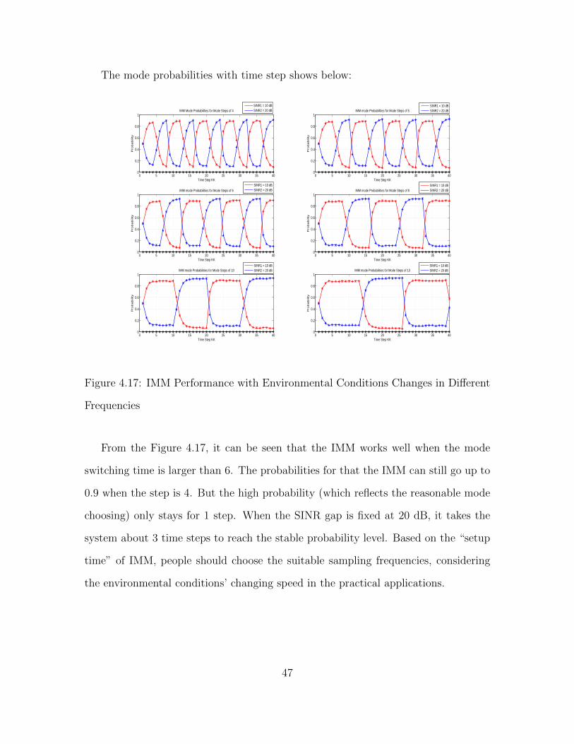
The mode probabilities with time step shows below:

0 5 10 15 20 25 30 35 400

0.2

0.4

0.6

0.8

1

Time Step KK

Pro

bability

IMM Mode Probabilities for Mode Steps of 4


0 5 10 15 20 25 30 35 400

0.2

0.4

0.6

0.8

1

Time Step KK

Pro

bability

IMM mode Probabilities for Mode Steps of 5


0 5 10 15 20 25 30 35 400

0.2

0.4

0.6

0.8

1

Time Step KK

Pro

bability



0 5 10 15 20 25 30 35 400

0.2

0.4

0.6

0.8

1

Time Step KK

Pro

bability



0 5 10 15 20 25 30 35 400

0.2

0.4

0.6

0.8

1

Time Step KK

Pro

bability



0 5 10 15 20 25 30 35 400

0.2

0.4

0.6

0.8

1

Time Step KK

Pro

bability



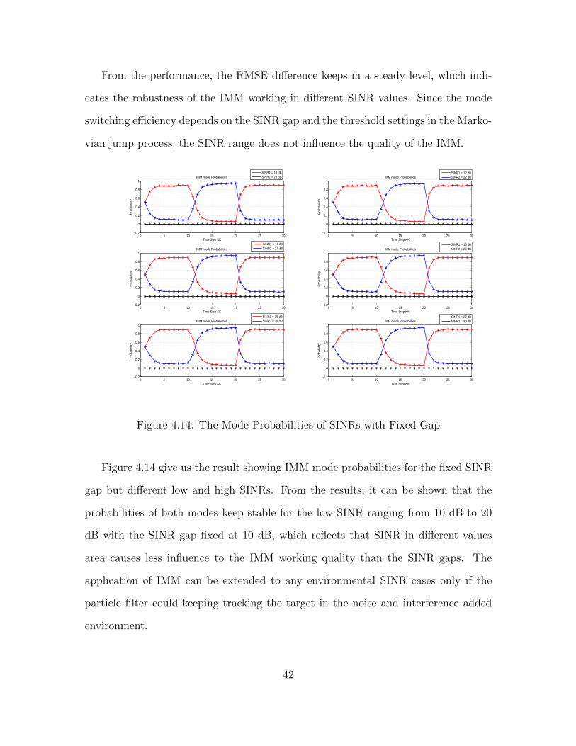
Figure 4.17: IMM Performance with Environmental Conditions Changes in Different

Frequencies

From the Figure 4.17, it can be seen that the IMM works well when the mode

switching time is larger than 6. The probabilities for that the IMM can still go up to

0.9 when the step is 4. But the high probability (which reflects the reasonable mode

choosing) only stays for 1 step. When the SINR gap is fixed at 20 dB, it takes the

system about 3 time steps to reach the stable probability level. Based on the “setup

time” of IMM, people should choose the suitable sampling frequencies, considering

the environmental conditions’ changing speed in the practical applications.

47

4.5 Three Interference Power Levels

This part of the simulation will show results that the IMM works with more than

two system modes. For the extension for IMM from two or more modes, we will focus

on the performance of IMM working with three modes. Also, an example of IMM

working with 4 modes will be presented at the end of this part.

To complete the simulation, 6 groups of SINRs will be chosen. The noise and

interference variances values are set with increasing SINRs with the same gap in

each group. And for different group, the SINR gap will gradually increase with the

continuing of the simulation. The variances values are shown in Table 4.7 :

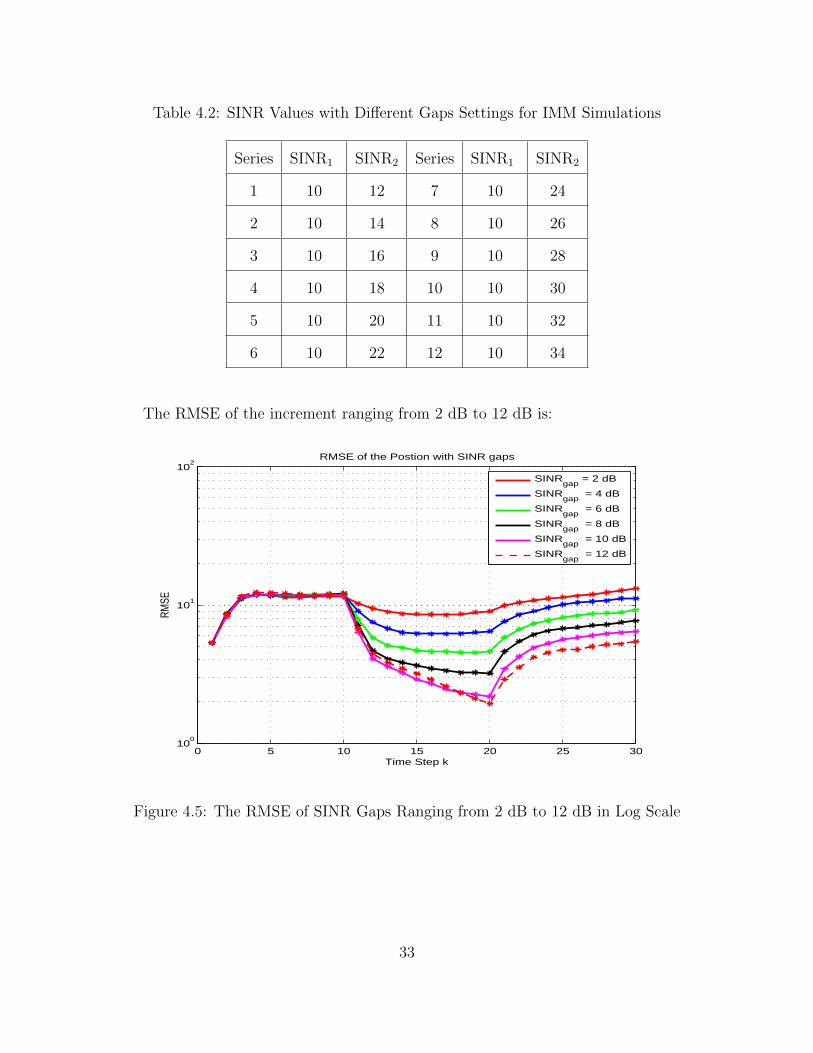
Table 4.7: SINR Values with Different Gaps Settings for IMM Simulations

Series SINR1 SINR2 SINR3

1 10 12 14

2 10 14 18

3 10 16 22

4 10 18 26

5 10 20 30

6 10 22 34


π =

0.8 0.1 0.1

0.1 0.8 0.1

0.1 0.1 0.8

(4.8)

The probabilities successively in each row represents the probability that the mode

switching to SINR1, SINR2, and SINR3. And probabilities successively in each column

represents the probability that the mode switching from SINR1, SINR2, and SINR3.

48

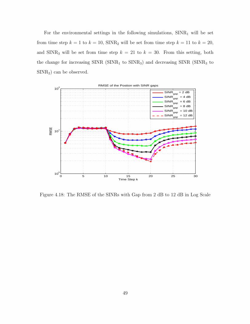
For the environmental settings in the following simulations, SINR1 will be set

from time step k = 1 to k = 10, SINR2 will be set from time step k = 11 to k = 20,

and SINR3 will be set from time step k = 21 to k = 30. From this setting, both

the change for increasing SINR (SINR1 to SINR3) and decreasing SINR (SINR3 to

SINR2) can be observed.

0 5 10 15 20 25 3010

0

101

102

Time Step k

RMSE


SINR

gap = 2 dB

SINRgap

= 4 dB

SINRgap

= 6 dB

SINRgap

= 8 dB

SINRgap

= 10 dB

SINRgap

= 12 dB

Figure 4.18: The RMSE of the SINRs with Gap from 2 dB to 12 dB in Log Scale

49

0 5 10 15 20 25 300

2

4

6

8

10

12

14

Time Step k

RMSE


SINRgap

= 2 dB

SINRgap

= 4 dB

SINRgap

= 6 dB

SINRgap

= 8 dB

SINRgap

= 10 dB

SINRgap

= 12 dB

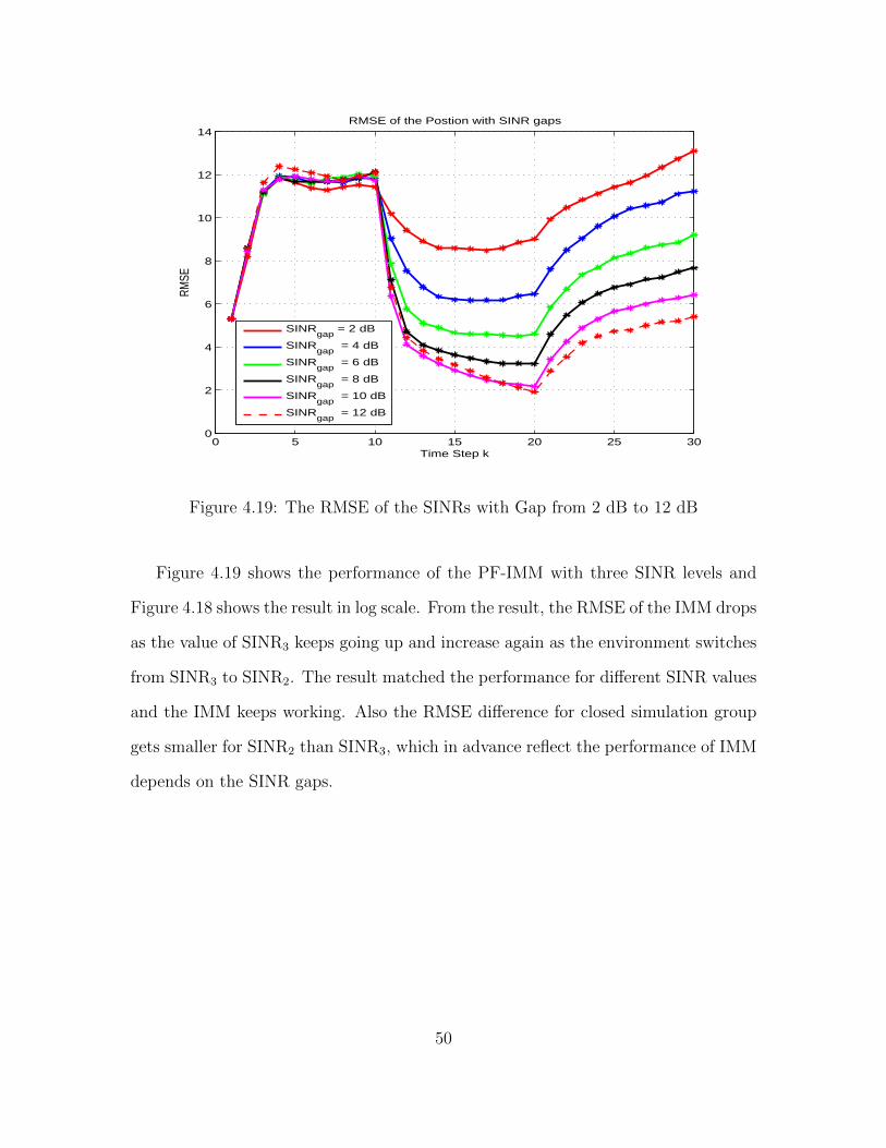
Figure 4.19: The RMSE of the SINRs with Gap from 2 dB to 12 dB

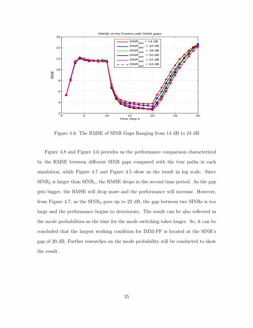
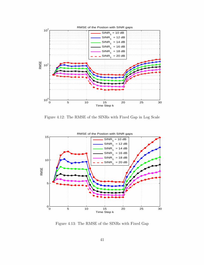
Figure 4.19 shows the performance of the PF-IMM with three SINR levels and

Figure 4.18 shows the result in log scale. From the result, the RMSE of the IMM drops

as the value of SINR3 keeps going up and increase again as the environment switches

from SINR3 to SINR2. The result matched the performance for different SINR values

and the IMM keeps working. Also the RMSE difference for closed simulation group

gets smaller for SINR2 than SINR3, which in advance reflect the performance of IMM

depends on the SINR gaps.

50

0 5 10 15 20 25 300

0.2

0.4

0.6

0.8

1

Time Step KK

Prob

abilit

y


SINR1 = 10 dBSINR2 = 12 dBSINR3 = 14 dB

0 5 10 15 20 25 300

0.2

0.4

0.6

0.8

1

Time Step KK

Prob

abilit

y



0 5 10 15 20 25 300

0.2

0.4

0.6

0.8

1

Time Step KK

Prob

abilit

y



0 5 10 15 20 25 300

0.2

0.4

0.6

0.8

1

Time Step KK

Prob

abilit

y



0 5 10 15 20 25 300

0.2

0.4

0.6

0.8

1

Time Step KK

Prob

abilit

y



0 5 10 15 20 25 300

0.2

0.4

0.6

0.8

1

Time Step KK

Prob

abilit

y



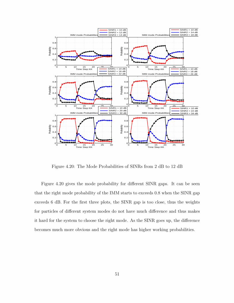
Figure 4.20: The Mode Probabilities of SINRs from 2 dB to 12 dB

Figure 4.20 gives the mode probability for different SINR gaps. It can be seen

that the right mode probability of the IMM starts to exceeds 0.8 when the SINR gap

exceeds 6 dB. For the first three plots, the SINR gap is too close, thus the weights

for particles of different system modes do not have much difference and thus makes

it hard for the system to choose the right mode. As the SINR goes up, the difference

becomes much more obvious and the right mode has higher working probabilities.

51

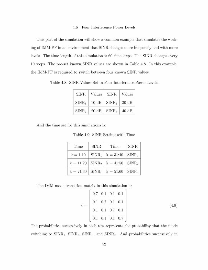
4.6 Four Interference Power Levels

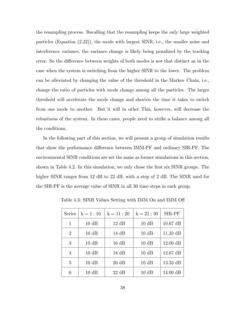
This part of the simulation will show a common example that simulates the work-

ing of IMM-PF in an environment that SINR changes more frequently and with more

levels. The time length of this simulation is 60 time steps. The SINR changes every

10 steps. The pre-set known SINR values are shown in Table 4.8. In this example,

the IMM-PF is required to switch between four known SINR values.

Table 4.8: SINR Values Set in Four Interference Power Levels

SINR Values SINR Values

SINR1 10 dB SINR3 30 dB

SINR2 20 dB SINR4 40 dB

And the time set for this simulations is:

Table 4.9: SINR Setting with Time

Time SINR Time SINR

k = 1:10 SINR1 k = 31:40 SINR3

k = 11:20 SINR2 k = 41:50 SINR2

k = 21:30 SINR1 k = 51:60 SINR4


π =

0.7 0.1 0.1 0.1

0.1 0.7 0.1 0.1

0.1 0.1 0.7 0.1

0.1 0.1 0.1 0.7

(4.9)

The probabilities successively in each row represents the probability that the mode

switching to SINR1, SINR2, SINR3, and SINR4. And probabilities successively in

52

each column represents the probability that the mode switching from SINR1, SINR2,

SINR3, and SINR4.

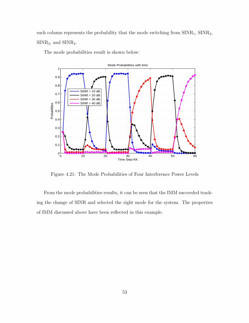
The mode probabilities result is shown below:

0 10 20 30 40 50 600

0.1

0.2

0.3

0.4

0.5

0.6

0.7

0.8

0.9

1

Time Step KK

Pro

babi

litie

s

Mode Probabilities with time

SINR = 10 dBSINR = 20 dBSINR = 30 dBSINR = 40 dB

Figure 4.21: The Mode Probabilities of Four Interference Power Levels

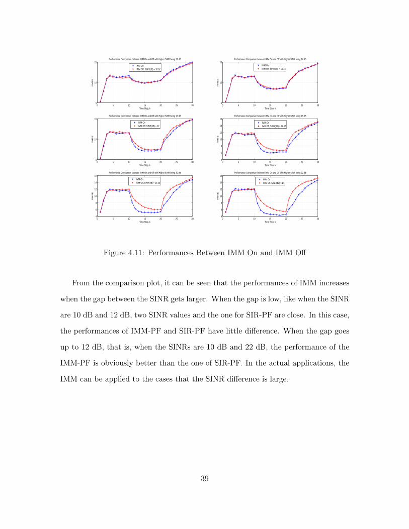
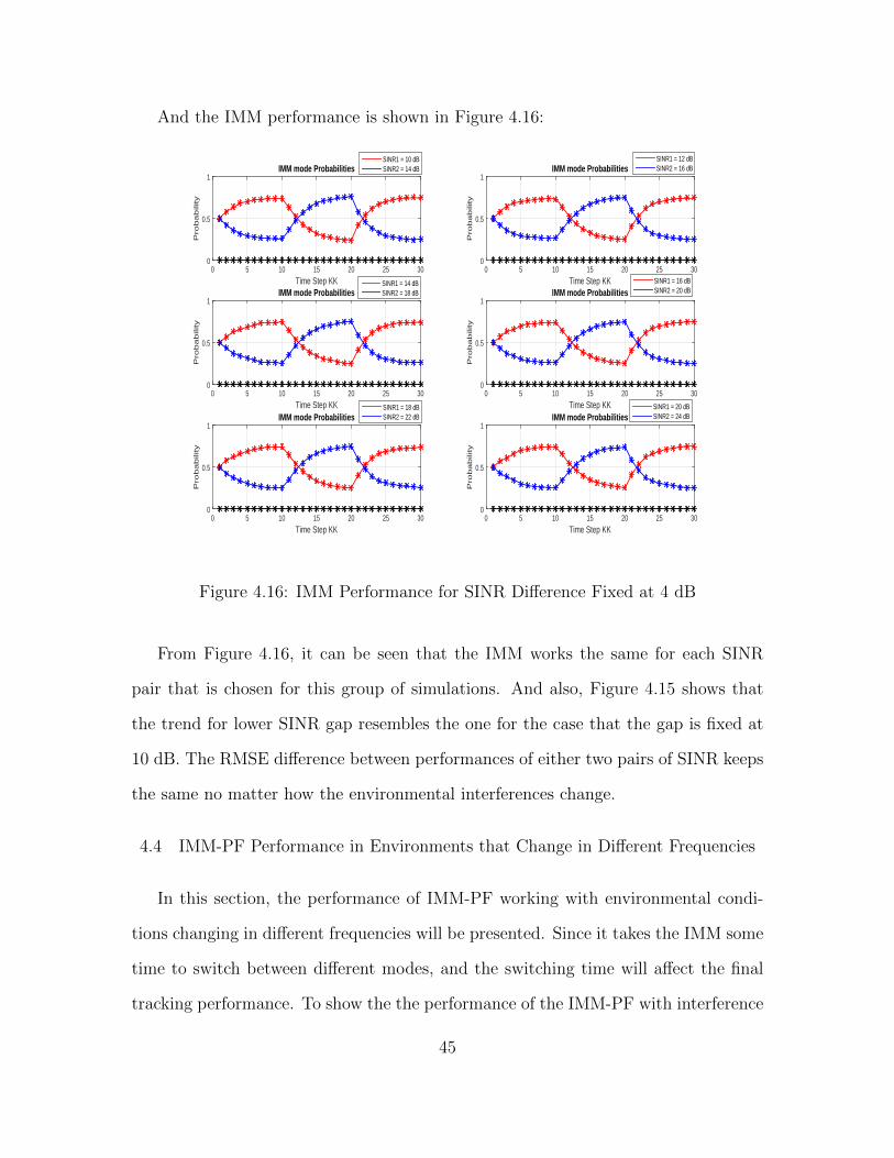
From the mode probabilities results, it can be seen that the IMM succeeded track-

ing the change of SINR and selected the right mode for the system. The properties

of IMM discussed above have been reflected in this example.

53

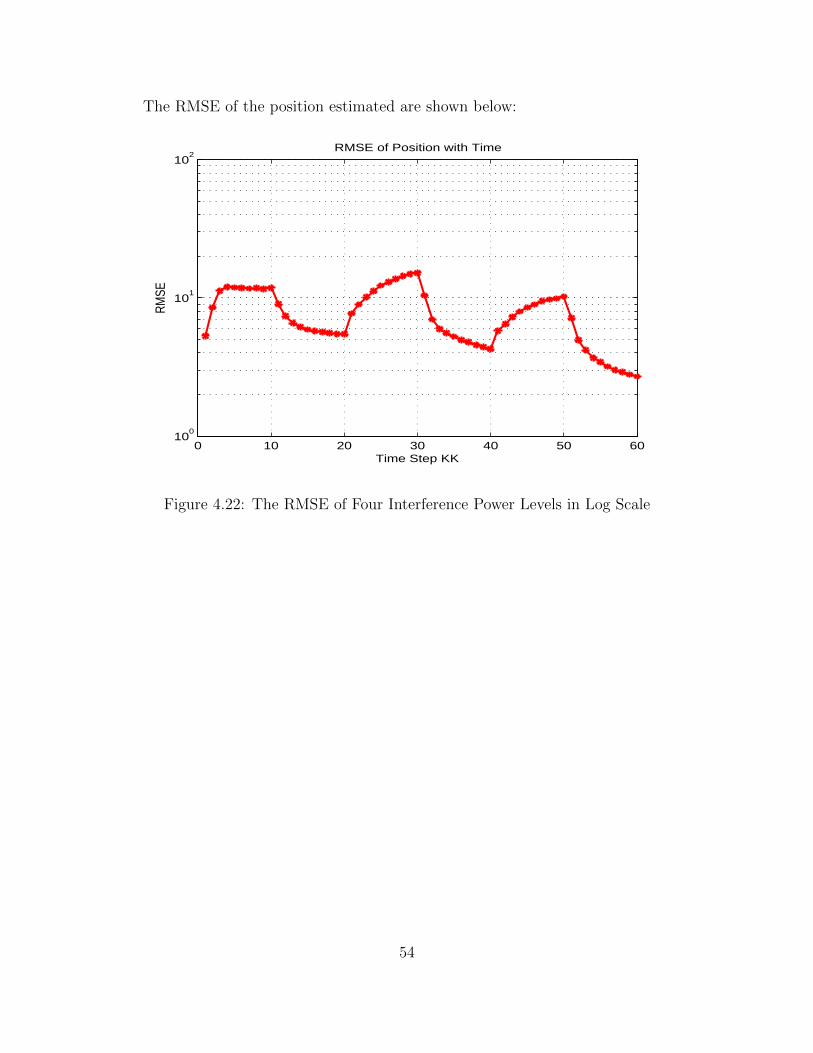
The RMSE of the position estimated are shown below:

0 10 20 30 40 50 6010

0

101

102

RMSE of Position with Time

Time Step KK

RMSE

Figure 4.22: The RMSE of Four Interference Power Levels in Log Scale

54

0 10 20 30 40 50 602

4

6

8

10

12

14

16RMSE of Position with Time

Time Step KK

RMSE

Figure 4.23: The RMSE of Four Interference Power Levels

Figure 4.23 gives us the result of the RMSE of the position estimation results by

IMM-PF and Figure 4.22 has shown the result in log scale. It can be seen that the

RMSE trend approximates the change of the SINR. This example proves in advance

the adaptation for the IMM-PF for real environments.

55

Chapter 5

EXTENSION TO ESTIMATING VARIANCE DYNAMICALLY

5.1 Scenario Settings

In some environments, the interference and noise power levels vary dynamically

and the values are not known. In these cases of target tracking applications, the

linear chirp is adopted for the radar signal to detect the target. The range and range

rate information are embedded in the linear frequency modulation chirp shown in the

equation below:

s(t) = cos(2π(k

2(t− τ)2) + 2πν(t− τ)) (5.1)

r(t) = As(t) + w(t) + c(t). (5.2)

The signal is transmitted from the radar. If the target exists, the reflected signal

will be sent back. The receiving signal is supposed to have the form of Equation

(5.2). In this equation, w(t) denotes the additive white Gaussian noise (AWGN), and

c(t) denotes the communications interference. By analyzing the time delays and the

Doppler shifts, the range and the range rate of the target can be determined. This

process can be divided into two parts: one is to analyze the return signal, extract the

time delays and the Doppler shifts from the signal that is added with white noise and

the communications interference. The other is to estimate the target position and

velocity state from the time delay and the Doppler shift.

To determine if the reflected signal is present, we will construct the generalised

likelihood ratio test (GLRT) using the maximum likelihood estimates (MLE) of the

time delay τ , Doppler shift ν, signal amptitude A, and environmental variance σ.

56

The MLE of the parameters are found by maximizing the probability density function

(PDF) under the hypothesises that the target is present.

In Equation (5.1), τ represents the time delay, ν represents the Doppler shift. In

the target detection case, the amplitude A, chirp rate k, and initial frequency f0 are

assuming to be known. The target location and its moving velocity are found from

the estimated values of τ and ν. The principal approach to designing a good detector

for this composite hypothesis testing problem is to set up the GLRT [44].

Supposed the sampled transmitted signal has the following form:

s[n] = cos(2πfc(n− n0)2 + 2πν0(n− n0)) (5.3)

Consider the problem in this case:

H0 : x[n] = w0[n] n = 0, 1, ..., N − 1

H1 : x[n] = As[n] + w1[n] n = 0, 1, ..., N − 1

In Hypothesis H1, the amplitude A, arrival time n0, Doppler shift ν0 and variance

σ21 are unknown. Suppose the MLE of these parameters are A, n0, ν0 and σ2

1. In

Hypothesis H0, the variance σ20 is unknown and suppose the MLE is σ2

0. Take these

MLE into the expression for s[n]

s[n] = cos(2πf0(n− n0)2 + 2πν0(n− n0))

The MLE of A for is given by [9]:

A =

∑N−1n=0 x[n]s[n]∑N−1n=0 s

2[n](5.4)

The expression for the MLE of two variances are:

σ21 =

1

N

N−1∑n=0

[x[n]− As[n]]2

57

σ20 =

1

N

N−1∑n=0

(x[n])2

The PDF for H1 is:

p(x; H1 : A, n0, ν0, σ21)

=1

(2πσ21)

N2

exp(−∑N−1

n=0 (x[n]− As[n; n0, ν0])2

2σ21

)

And the PDF for H0 is:

p(x; H0 : σ20)

=1

(2πσ20)

N2

exp(−∑N−1

n=0 (x[n])2

2σ20

)

The detector for GLRT is as the ratio of likelihood functions under each hypothesisl.

Hypothesis H1 is detected if

LG(x)p(x; H1 : A, ν0, n0, σ

21)

p(x; H0 : σ20)

> γ

5.2 GLRT and MLE Computation

The GLRT test statistic can be simplified as:

T (x) =p(x; H1 : A, n0, ν0, σ

21)

p(x; H0 : σ20)

=

1

(2πσ21)N2

exp(−∑N−1n=0 (x[n]−As[n;n0,ν0])2

2σ21

)

1

(2πσ20)N2

exp(−∑N−1n=0 (x[n])2

2σ20

)

The MLE of variances σ20 and σ2

1 can be taken to simplify the exponential parts in

both the numerator and the denominator:

T (x) =(2πσ2

0)N2

(2πσ21)

N2

·exp(−N

2)

exp(−N2

)

=(2πσ2

0)N2

(2πσ21)

N2

=(σ2

0)N2

(σ21)

N2

58

Let

T ′(x) =N2

√T (x)

T ′(x) =σ20

σ21

>N2

√LG(x)

Take the MLE of variances in

=1N

∑N−1n=0 (x[n])2

1N

∑N−1n=0 (x[n]− As[n; n0, ν0])2

=

∑N−1n=0 (x[n])2∑N−1

n=0 (x[n])2 − 2A∑N−1

n=0 x[n]s[n; n0, ν0] +∑N−1

n=0 (s[n; A, n0, ν0])2

Take the expression of s[n; A, n0, ν0] into part of the denominator

2N−1∑n=0

x[n]s[n; A, n0, ν0]−N−1∑n=0

(s[n; A, n0, ν0])2

= 2AN−1∑n=0

s[n]− A2

N−1∑n=0

(s[n])2

Take the expression of the MLE of A inside the equation:

A =

∑N−1n=0 x[n]s[n]∑N−1n=0 s

2[n]

The above equation:

2AN−1∑n=0

s[n]− A2

N−1∑n=0

(s[n])2

= 2(∑N−1

n=0 x[n]s[n])2∑N−1n=0 s

2[n]

−(∑N−1

n=0 x[n]s[n])2

(∑N−1

n=0 s2[n])2

·N−1∑n=0

s2[n]

= 2(∑N−1

n=0 x[n]s[n])2∑N−1n=0 s

2[n]− (∑N−1

n=0 x[n]s[n])2∑N−1n=0 s

2[n]

=(∑N−1

n=0 x[n]s[n])2∑N−1n=0 s

2[n]

59

So, the right part in the denominator is:

= 2AN−1∑n=0

s[n]− A2

N−1∑n=0

(s[n])2

=(∑N−1

n=0 x[n]s[n])2∑N−1n=0 s

2[n]

It can be shown that∑N−1n=0 x[n]s[n]√

var(x[n])√∑N−1

n=0 s2[n]

is a Gaussian distribution.

Let

u(x) =

∑N−1n=0 x[n]s[n]√

var(x[n])√∑N−1

n=0 s2[n]

u(x) ∼ N(0, 1) under H0

u(x) ∼ N(

√∑N−1n=0 s

2[n]

var(x[n]), 1) under H1

So [u(x)]2 is a Chi-square distribution:

[u(x)]2 ∼ χ21 under H0

[u(x)]2 ∼ χ′21(λ) under H1

λ =

√∑N−1n=0 s

2[n]

var(x[n])

After acquiring the distribution of u[x], we can go back to the detector:

T ′(x) =

∑N−1n=0 x

2[n]∑N−1n=0 x

2[n]− [u(x)]2

The MLE of ν0 and n0 can be found by maximizing the expression of T ′(x).

ν0, n0 = arg maxν0,n0

∑N−1n=0 x

2[n]∑N−1n=0 x

2[n]− [u(x)]2

Since∑N−1

n=0 x2[n] is fixed for each iteration, the only thing varied is

∑N−1n=0 [u(x)]2. So

we only need to maximize:

ν0, n0 = arg maxν0,n0

[u(x)]2

In this way , the MLE of A, n0, ν0 can be found.

60

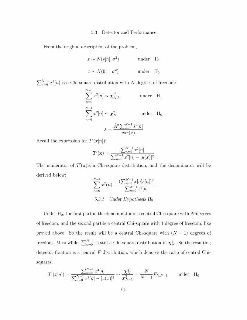
5.3 Detector and Performance

From the original description of the problem,

x ∼ N(s[n], σ2) under H1

x ∼ N(0, σ2) under H0∑N−1n=0 x

2[n] is a Chi-square distribution with N degrees of freedom:

N−1∑n=0

x2[n] ∼ χ′2N(λ) under H1

N−1∑n=0

x2[n] ∼ χ2N under H0

λ =A2∑N−1

n=0 s2[n]

var(x)

Recall the expression for T ′(x[n]):

T ′(x) =

∑N−1n=0 x

2[n]∑N−1n=0 x

2[n]− [u(x)]2

The numerator of T ′(x)is a Chi-square distribution, and the denominator will be

derived below:N−1∑n=0

x2(n)− (∑N−1

n=0 x[n]s[n])2∑N−1n=0 s

2[n]

5.3.1 Under Hypothesis H0

Under H0, the first part in the denominator is a central Chi-square with N degrees

of freedom, and the second part is a central Chi-square with 1 degree of freedom, like

proved above. So the result will be a central Chi-square with (N − 1) degrees of

freedom. Meanwhile,∑N−1

n=0 is still a Chi-square distribution in χ2N . So the resulting

detector fraction is a central F distribution, which denotes the ratio of central Chi-

squares.

T ′(x[n]) =

∑N−1n=0 x

2[n]∑N−1n=0 x

2[n]− [u(x)]2∼ χ2

N

χ2N−1

=N

N − 1FN,N−1 under H0

61

To make the detector a standard F distribution, we can move the coefficient NN−1 to

the detector

T ′′(x[n]) =N − 1

NT ′(x[n])

T ′′(x[n]) ∼ FN,N−1 under H0

5.3.2 Under Hypothesis H1

In hypothesis H1, we can take x[n] = As[n; n0, ν0] + w[n; σ21] into the expression:

T ′(x) =

∑N−1n=0 x

2[n]∑N−1n=0 x

2[n]− (∑N−1n=0 x[n]s[n])

2∑N−1n=0 s

2[n]

It can be seen that the nominator,∑N−1

n=0 x2[n], is a non-central Chi-square with the

N degrees of freedom and λ =A2

∑N−1n=0 s

2[n]1N

∑N−1n=0 (x2[n]−s2[n]) . The denominator will be analyzed

below:N−1∑n=0

x2[n]

=N−1∑n=0

(As[n; n0, ν0] + w[n; σ21])2

= A2

N−1∑n=0

s2[n] + 2AN−1∑n=0

s[n]w[n] +N−1∑n=0

w2[n]

And,

(∑N−1

n=0 x[n]s[n])2∑N−1n=0 s

2[n]

=

∑N−1n=0 ((As[n] + w[n])s[n])2∑N−1

n=0 s2[n]

=(A∑N−1

n=0 s2[n] +

∑N−1n=0 w[n]s[n])2∑N−1

n=0 s2[n]

=A2(∑N−1

n=0 s2[n])2 + 2A

∑N−1n=0 s

2[n]∑N−1

n=0 w[n]s[n] + (∑N−1

n=0 w[n]s[n])2∑N−1n=0 s

2[n]

62

= A2

N−1∑n=0

s2[n] + 2AN−1∑n=0

w[n]s[n]

+(∑N−1

n=0 w[n]s[n])∑N−1n=0 s

2[n]

Then, subtracting the two:

N−1∑n=0

x2[n]− (∑N−1

n=0 x[n]s[n])2∑N−1n=0 s

2[n]

= A2

N−1∑n=0

s2[n] + 2AN−1∑n=0

s[n]w[n] +N−1∑n=0

w2[n]

−(A2

N−1∑n=0

s2[n] + 2AN−1∑n=0

s[n]w[n] +(∑N−1

n=0 w[n]s[n])2∑N−1n=0 s

2[n])

=N−1∑n=0

w2[n]− (∑N−1

n=0 w[n]s[n])2∑N−1n=0 s

2[n]

It can be seen that the simplified result of the denominator is the same from the one

in H0. So it is a central Chi-square with (N − 1) degrees of freedom.

T ′′(x[n]) =N − 1

N

χ2N(λ)

χ2N−1∼ FN,N−1(λ)

T ′′(x[n]) ∼ F ′N,N−1(λ) under H1

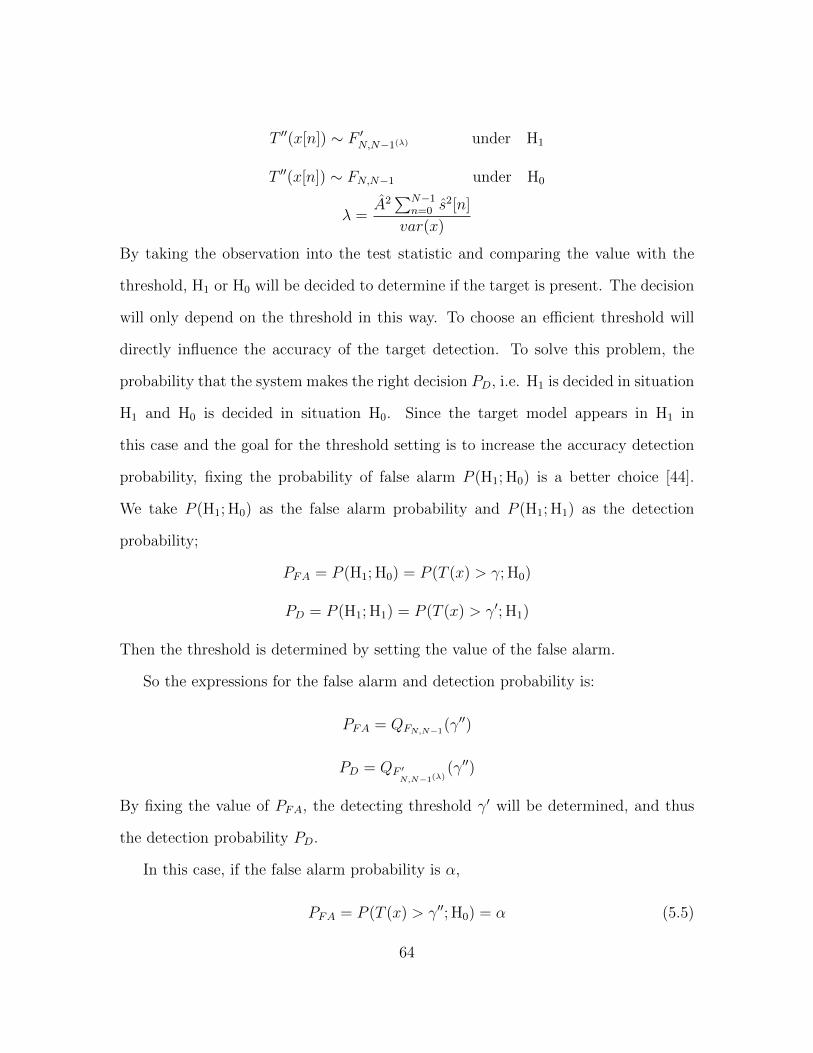
5.4 Performance

From the above derivations, it is clear that the distribution of T ′′(x[n]) is a F

distribution, which is denoted as the ratio of Chi-square.

63

T ′′(x[n]) ∼ F ′N,N−1(λ) under H1

T ′′(x[n]) ∼ FN,N−1 under H0

λ =A2∑N−1

n=0 s2[n]

var(x)

By taking the observation into the test statistic and comparing the value with the

threshold, H1 or H0 will be decided to determine if the target is present. The decision

will only depend on the threshold in this way. To choose an efficient threshold will

directly influence the accuracy of the target detection. To solve this problem, the

probability that the system makes the right decision PD, i.e. H1 is decided in situation

H1 and H0 is decided in situation H0. Since the target model appears in H1 in

this case and the goal for the threshold setting is to increase the accuracy detection

probability, fixing the probability of false alarm P (H1; H0) is a better choice [44].

We take P (H1; H0) as the false alarm probability and P (H1; H1) as the detection

probability;

PFA = P (H1; H0) = P (T (x) > γ; H0)

PD = P (H1; H1) = P (T (x) > γ′; H1)

Then the threshold is determined by setting the value of the false alarm.

So the expressions for the false alarm and detection probability is:

PFA = QFN,N−1(γ′′)

PD = QF ′N,N−1(λ)

(γ′′)

By fixing the value of PFA, the detecting threshold γ′ will be determined, and thus

the detection probability PD.

In this case, if the false alarm probability is α,

PFA = P (T (x) > γ′′; H0) = α (5.5)

64

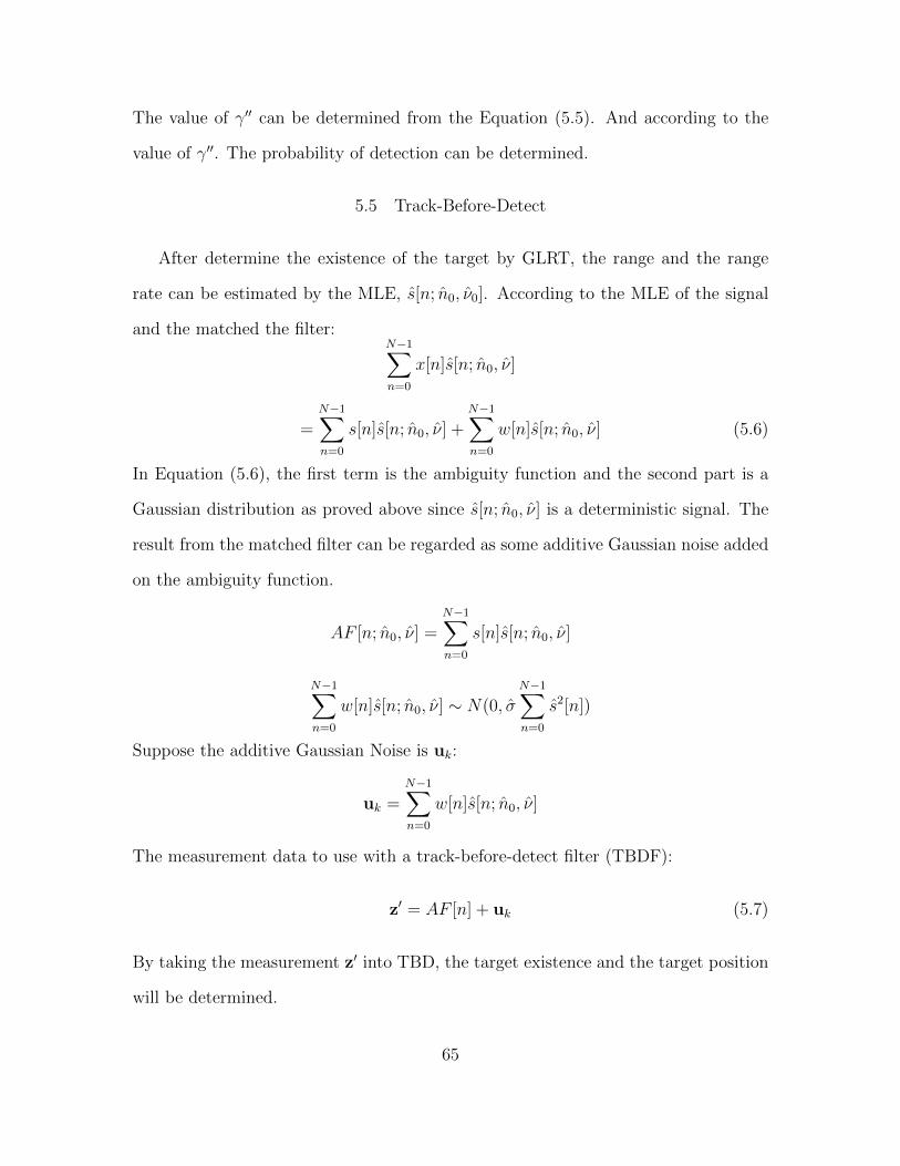
The value of γ′′ can be determined from the Equation (5.5). And according to the

value of γ′′. The probability of detection can be determined.

5.5 Track-Before-Detect

After determine the existence of the target by GLRT, the range and the range

rate can be estimated by the MLE, s[n; n0, ν0]. According to the MLE of the signal

and the matched the filter:N−1∑n=0

x[n]s[n; n0, ν]

=N−1∑n=0

s[n]s[n; n0, ν] +N−1∑n=0

w[n]s[n; n0, ν] (5.6)

In Equation (5.6), the first term is the ambiguity function and the second part is a

Gaussian distribution as proved above since s[n; n0, ν] is a deterministic signal. The

result from the matched filter can be regarded as some additive Gaussian noise added

on the ambiguity function.

AF [n; n0, ν] =N−1∑n=0

s[n]s[n; n0, ν]

N−1∑n=0

w[n]s[n; n0, ν] ∼ N(0, σN−1∑n=0

s2[n])

Suppose the additive Gaussian Noise is uk:

uk =N−1∑n=0

w[n]s[n; n0, ν]

The measurement data to use with a track-before-detect filter (TBDF):

z′ = AF [n] + uk (5.7)

By taking the measurement z′ into TBD, the target existence and the target position

will be determined.

65

Chapter 6

CONCLUSIONS AND FUTURE WORK

6.1 Conclusions

In this thesis, the interacting multiple model (IMM) is adopted as a modification

to the particle filter, to make the tracking system adapt to the dynamic changes

in the power level of interference. In this algorithm, a finite-number state variable

is incorporated in the particle filter to represent the particles’ filter modes which

are set to work for different environmental conditions. Simulation results show that

the tracking accuracy of the particle filter will be improved when integrated with

the IMM. Meanwhile, results also show that the quality of the IMM depends on the

transfer probabilities in the Markov process matrix (MPM). Different MPM probabil-

ities result in the varied number of particles working at the right mode, thus affecting

the stability of the target tracking. Also, the differences between the possible SINR

values also affect the system tracking performances. As the SINR gap increases, the

IMM-PF result in less RMSE, owing to the larger difference in mode probabilities.

We have also considered the scenario where the power level of the interference

is not known at each time step. In this case, the GLRT is implemented to detect

the signal. The target states’ parameters and the variances of the environmental

conditions are estimated by the MLE before the GLRT is constructed. Once the

estimated interference power level is obtained, based on the estimated value, it can

be incorporated into a track-before-detect filter (TBDF) to complete the tracking

processes.

66

6.2 Future Work

According to the studies related to the IMM-PF, there are some area that can be

modified:

• In this work, the SINR gap of the known SINR values are supposed to be at

least 5 dB. More work can be done to improve the performance of IMM to work

better in the cases where the SINR gap is lower. This modification would make

the IMM applicable in more real scenarios, where the SINR changes gradually.

• This work defined the SINR directly using the true state as the signal power

which is not achievable in actual situations. Continuing work can be focused

on extending this to real applications where a specific form of signal, like the

linear chirp used in the GLRT part of this thesis, to detect the target.

• Derivations for the GLRT have been presented in this thesis to detect the target

using the linear chirp radar signal in high interference power levels cases. Sim-

ulations will be required to prove the derivation and show the performances of

the target detection and tracking. The detection performances can be evaluated

by the false alarm and detection probabilities. The tracking performance can

be evaluated using the mean-squared error metric.

• The track-before-detect filter (TBDF) can be used in detection and target track-

ing in higher interference environments when the GLRT with the linear chirp

fails to detect the existence of the target. Unlike the normal TBDF where the

environmental interference and noise variance is fixed, the IMM can be inte-

grated with the TBDF to allow for varying environmental conditions.

67

REFERENCES

[1] J. P. Singh, “Evolution of the radar target tracking algorithms: a move to-wards knowledge based multi-sensor adaptive processing,” IEEE InternationalWorkshop on Computational Advances in Multi-Sensor Adaptive Processing, pp.40–43, December 2005.

[2] I. Skolnik, Merrill, “Introduction to radar,” Radar Handbook, vol. 2, 1962.

[3] E. S. Abdoul-Moaty, T. R. Abdoul-Shahid, A. El-Din Sayed Hafez, and M. Abd-El-Latif, “A particle filter for mutistatic radar tracking,” IEEE Aerospace Con-ference, pp. 1–5, March 2014.

[4] J. Neyman and E. S. Pearson, On the Problem of the Most Efficient Tests ofStatistical Hypotheses. Springer, 1992.

[5] M. A. Richards, Fundamentals of Radar Signal Processing. Tata McGraw-HillEducation, 2005.

[6] D. F. Bizup and D. E. Brown, “Maneuver detection using the radar range ratemeasurement,” IEEE Transactions on Aerospace and Electronic Systems, vol. 40,no. 1, pp. 330–336, 2004.

[7] B. Ristic, S. Arulampalam, and N. Gordon, Beyond the Kalman Filter: ParticleFilters for Tracking Applications. Boston: Artech House, 2004, vol. 685.

[8] F. Orderud, “Comparison of Kalman filter estimation approaches for state spacemodels with nonlinear measurements,” in Proceedings of Scandinavian Confer-ence on Simulation and Modeling, 2005, pp. 1–8.

[9] S. M. Kay, Fundamentals of Statistical Signal Processing: Estimation Theory.Prentice-Hall PTR, 1993.

[10] I. B. Rhodes, “A tutorial introduction to estimation and filtering,” IEEE Trans-actions on Automatic Control, vol. 16, no. 6, pp. 688–706, 1971.

[11] A. H. Jazwinski, Stochastic Processes and Filtering Theory. Courier Corpora-tion, 2007.

[12] A. Gelb, Applied Optimal Estimation. MIT press, 1974.

[13] E. A. Wan and R. Van Der Merwe, “The unscented Kalman filter for nonlinearestimation,” in The IEEE Adaptive Systems for Signal Processing, Communica-tions, and Control Symposium, 2000, pp. 153–158.

[14] S. Julier, J. Uhlmann, and H. F. Durrant-Hyte, “A new method for the non-linear transformation of means and covariances in filters and estimators,” IEEETransactions on Automatic Control, vol. 45, no. 3, pp. 477–482, March 2000.

68

[15] M. S. Arulampalam, S. Maskell, N. Gordon, and T. Clapp, “A tutorial on particlefilters for online nonlinear/non-Gaussian Bayesian tracking,” IEEE Transactionson Signal Processing, vol. 50, no. 2, pp. 174–188, February 2002.

[16] A. Yonis, M. Abdullah, and M. Ghanim, “LTE-FDD and LTE-TDD for cellularcommunications,” Progress In Electromagnetics Research Symposium Proceed-ings, pp. 1467–1471, 2012.

[17] S. Stefania, T. Issam, and B. Matthew, LTE, The UMTS Long Term Evolutionfrom Theory to Practice, 2nd ed. John Wiley & Sons, Ltd, 2011.

[18] M. Ishibashi, Y. Iwashita, and R. Kurazume, “Noise-estimate particle PHD fil-ter,” in World Automation Congress, 2014, pp. 784–789.

[19] J. Chen and L. Ma, “Particle filtering with correlated measurement and processnoise at the same time,” IET Radar, Sonar & Navigation, vol. 5, no. 7, pp.726–730, 2011.

[20] P. M. Djuric and J. Miguez, “Sequential particle filtering in the presence ofadditive Gaussian noise with unknown parameters,” in IEEE International Con-ference on Acoustics, Speech, and Signal Processing, vol. 2, 2002, pp. 1621–1624.

[21] H. A. Blom and Y. Bar-Shalom, “The interacting multiple model algorithm forsystems with Markovian switching coefficients,” IEEE Transactions on Auto-matic Control, vol. 33, no. 8, pp. 780–783, 1988.

[22] S. M. Aly, R. El Fouly, and H. Braka, “Extended Kalman filtering and interactingmultiple model for tracking maneuvering targets in sensor netwotrks,” in IEEEWorkshop on Intelligent Solutions in Embedded Systems, 2009, pp. 149–156.

[23] J. D. Glass, W. Blair, and Y. Bar-Shalom, “IMM estimators with unbiasedmixing for tracking targets performing coordinated turns,” in IEEE AerospaceConference, 2013, pp. 1–10.

[24] M. Mallick and B. F. La Scala, “IMM estimator for ground target tracking withvariable measurement sampling intervals,” in IEEE International Conference onInformation Fusion, 2006, pp. 1–8.

[25] G. Shuli, W. Honglan, T. Cheng, and H. Shengguo, “Tracking maneuveringtarget on airport surface based on IMM-UKF algorithm,” in IEEE InternationalConference on Optoelectronics and Image Processing, vol. 2, 2010, pp. 671–675.

[26] N. Mohanty, “Computer tracking of moving point targets in space,” IEEE Trans-actions on Pattern Analysis and Machine Intelligence, no. 5, pp. 606–611, 1981.

[27] J. D. R. Kramer Jr and W. S. Reid, “Track-before-detect processing for anairborne type radar,” in IEEE International Radar Conference, 1990, pp. 422–427.

69

[28] P. C. Wei, B. Zeidler, and W. Ku, “Characterization of the performance ofthe track-before-detect approach to moving target detection,” in IEEE NationalAerospace and Electronics Conference, 1992, pp. 275–279.

[29] S. J. Davey, M. G. Rutten, and B. Cheung, “A comparison of detection per-formance for several track-before-detect algorithms,” EURASIP Journal on Ad-vances in Signal Processing, vol. 2008, p. 41, 2008.

[30] M. West and J. Harrison, Bayesian Forecasting and Dynamic Models, 2nd ed.New York: Springer-Verlag, 1997, vol. 18.

[31] J. E. Handschin, “Monte Carlo techniques for prediction and filtering of non-linear stochastic processes,” Automatica, vol. 6, no. 4, pp. 555–563, 1970.

[32] P. M. Djuric, F. M. Bugallo, J. H. Kotecha, J. Zhang, Y. Huang, T. Ghirmai,and J. Miguez, “Particle filtering,” IEEE Signal Processing Magazine, vol. 20,no. 5, pp. 19–38, 2003.

[33] B. D. O. Alspach and J. B. Moore, Optimal Filtering. Mineola, NY: DoverPublications Inc., 1979.

[34] D. L. Alspach and H. W. Sorenson, “Nonlinear Bayesian estimation using Gaus-sian sum approximation,” IEEE Transaction on Automatic Control, vol. 17,no. 4, pp. 439–448, 1972.

[35] ——, “Recursive Bayesian estimation using Gaussian sums,” Automatica, vol. 7,no. 4, pp. 465–479, 1971.

[36] A. C. Harvey, Forecasting, Structural Time Series Models and the Kalman Filter.Cambridge: Cambridge University Press, 1990.

[37] A. H. Jazwinski, Stochastic Processes and Filtering Theory. New York: Aca-demic Press, 1970.

[38] A. Doucet, M. West, and S. J. Godstill, “Methodology for Monte Carlo smooth-ing with application to time-varying autoregressions,” IEEE International Con-ference on Acoustics, Speech, and Signal Processing, vol. 2, no. 2, pp. 701–704,June 2000.

[39] A. Doucet, S. Godsill, and C. Andrieu, “On sequential Monte Carlo methods forBayesian filtering,” Statistics and Computing, vol. 10, no. 3, pp. 197–208, 2000.

[40] Y. Boers and J. N. Driessen, “Interacting multiple model particle filter,” IEERadar, Sonar & Navigation, vol. 150, pp. 344–349, 2003.

[41] P. H. Foo and G. W. Ng, “Combining the interacting multiple model methodwith particle filters for manoeuvring target tracking,” IET Radar, Sonar & Nav-igation, vol. 5, pp. 234–255, 2011.

[42] S. Bar-Shalom, S. Challa, and H. Blom, “IMM estimator versus optimal es-timator for hybrid systems,” IEEE Transactions On Aerospace and ElectronicSystems, vol. 41, no. 4, pp. 986–991, 2005.

70

[43] Y. Bar-Shalom and X. Li, Estimation and Tracking: Principles, Techniques, andSoftwares. Artech House, 1993.

[44] S. M. Kay, Fundamentals of Statistical Signal Processing. Englewood Cliffs, NJ:PTR Prentice-Hall, 1993.

71

Date post:	18-Apr-2018
Category:	Documents
Upload:	vuthuy
View:	220 times
Download:	1 times

Radar Target Tracking - ASU Digital Repository Target Tracking ... ABSTRACT As the demand for ......

Documents