1

RANDOM FRACTALS

Contributed chapter to volume New perspectives in stochactic geometry,edited by Wilfrid Kendall and Ilya Molchanov.

by Peter Morters, University of Bath.

The term fractal usually refers to sets which, in some sense, have a self-similarstructure. Already in the seventies of the last century Mandelbrot (1982) madea compelling case for the importance of this concept in mathematical modelling.Indeed, some form of self-similarity is common in random sets, in particularthose arising from stochastic processes. Therefore studying fractal aspects is animportant feature of modern stochastic geometry.

Early progress in fractal geometry often referred to sets with obvious self-similarity, like the fixed points of iterated function systems. These are toy exam-ples, tailor-made to study self-similarity in its tidiest form. An overview of theachievements in this period can be obtained from (Falconer, 2003).

Starting with the work of Taylor in the sixties, researchers were also lookingat sets, where self-similarity is more hidden. Such sets often arise in the contextof stochastic processes. A beautiful survey of the state of the art in the mid1980s, written by the protagonist in this area, is (Taylor, 1986). In the last tenyears interest in this area has increased considerably, powerful techniques havebeen developed, and very substantial progress has been made. Typical examplesof the fractals studied today are level sets of stochastic processes, the doublepoints of random curves, or the boundary of excursions of random fields. Theself-similar nature of these examples is typically less tidy and exploiting it meansentering deep into the geometry of the sets.

Very roughly speaking, a set is self-similar if it can be decomposed intoparts which look like scaled copies of the original set. This definition becomesparticularly powerful when ‘look like’ is interpreted in a statistical sense, i.e. if itcan be decomposed into parts which have (up to scaling) the same distributionas the whole set. This idea is naturally linked to trees: Starting from the rootwe identify the parts in the decomposition as the children of the root. Each partis itself a scaled copy of the whole picture and hence has a decomposition ofthe same kind as its parent, proceeding like this each point of the fractal has anatural address in the tree.

A crucial tool to bring the self-similarity of a random set to light is thereforeits representation in terms of a tree, or sometimes a process on a tree. This tech-nique has been exploited with great success in the last ten years and continuesto be a vital tool. My main aim in this chapter is to show that the first step inmany deep geometric problems for random sets is to find the self-similarity ofthe problem and capture it in form of a tree picture. This picture determines

2 Random fractals

the key direction of the argument, although the formalised proof often does notmake the tree structure explicit.

Questions in geometry are very often related to the size of sets. Other than inclassical geometry, random sets can often already be distinguished by the crudestmeasure of size, which is dimension. The most powerful concept of dimension, butby far not the only one, is Hausdorff dimension, introduced almost a century agoby Hausdorff (1918). This concept extends the classical notion of dimension toarbitrary metric spaces, allowing non-integer dimensions for sufficiently irregularsets. The notion is based on a family of measures Hs, s ≥ 0, the s-Hausdorffmeasures, which for integer values s = 1, 2, 3 coincide with the classical measuresof length, area, and volume. The Hausdorff dimension of a set A is the criticalvalue s > 0 where the function s 7→ Hs(A) jumps from infinity to zero. We donot give a precise definition of Hausdorff measure and dimension here, but referthe reader instead to the excellent book (Falconer, 2003).

The first section of this chapter is devoted to representing self-similarity interms of trees, and we initially confine ourselves to simple examples. We show howto obtain the Hausdorff dimension of a set from a suitable tree representationand apply this to finding the Hausdorff dimension of the zero set of a linearBrownian motion.

In the second section we move to more sophisticated examples and presenttwo more recent results on the fine structure of planar Brownian motion, whichmake great use of tree representations. On the one hand we look at the problemof the favourite sites, solved by Dembo, Peres, Rosen, and Zeitouni (2001), andon the other hand we study the multifractal spectrum of the intersection of twopaths, a result of Klenke and Morters (2005). In both cases, rather than givingdetails of the proof, we emphasise the underlying tree structure. We completethe section with a discussion of an open problem initialised by work of Bass,Burdzy, and Khoshnevisan (1994).

The second example introduces the notion of probability exponents, the gen-eral use of which we discuss in the third section. This particular aspect of randomfractals has gained momentum through the discovery of an explicit formula forthe intersection and disconnection exponents by Lawler, Schramm, and Werner(2001) and the subsequent award of the Fields medal to Werner in 2006. Herewe discuss work of Lawler (1996a) on the Hausdorff dimension of the Brownianfrontier and some closely related results.

1.1 Representing fractals by trees

There is no generally accepted definition of a statistically self-similar set, and wedo not attempt to give one. Instead, we define a class of statistically self-similarsets, the Galton-Watson fractals, which comprises a number of interesting exam-ples. We prove a formula for the Hausdorff dimension of Galton-Watson fractals,which gives us the opportunity to explore the relationship between branchingprocesses and self-similarity and introduce basic ideas about probability on trees.

Representing fractals by trees 3

The forthcoming book (Lyons and Peres, 2008) gives a comprehensive accountof this subject, on which much of this section is based.

1.1.1 Fractals and trees

We start with a general approach to capture the self-similar nature of fractalsby means of trees with weights, so called capacities, associated to the edges, andinvestigate how the Hausdorff dimension of the fractal can be derived from thetree and the capacities.

A tree T = (V, E) consists of a finite or countable set V of vertices and a setE ⊂ V × V of edges. For every v ∈ V the set of parents {w ∈ V : (w, v) ∈ E}consists of exactly one element, denoted by v, except for exactly one distinguishedelement, called the root ρ ∈ V , which has no parent. For every v ∈ V there is aunique self-avoiding path from the root to v, called the ancestral line, and thenumber of edges in this path is the generation |v| of the vertex v ∈ V . For everyvertex v ∈ V we assume that the set of children {w ∈ V : (v, w) ∈ E} is finite.

sibling

parent

child

root

marked

offspring

vertex

Fig. 1.1. A tree, with a vertex in the second generation marked; its ancestralline is dashed and the tree of its offspring shaded. One of its three siblings,and one of its two children are pointed out, as well as its parent and the root.

The offspring of a vertex v is the collection of vertices having v on theirancestral line. These vertices naturally form a subtree T (v) of T . The siblings ofv ∈ V are the vertices u 6= v with u = v. A sequence (v0, v1, . . .) of vertices suchthat v0 = ρ and vi = vi−1 for all i ≥ 1 is called a ray in the tree. The set ofrays in T is denoted by ∂T . Finally, a set Π ⊂ E is called a cutset if every rayincludes an edge from the set Π.

4 Random fractals

We now describe a way to represent sets by marked trees. Let T = (V, E)be an infinite tree and associate to each vertex v ∈ V a nonempty, compact setIv ⊂ R

d such that Iv = cl(

int Iv

)

and

• if v is a child of u, then Iv ⊂ Iu;

• if u and v are siblings, then int Iu ∩ int Iv = ∅;• for all rays ξ = (v0, v1, . . .) we have lim

n→∞diam(Ivn

) = 0.

Then the setI(T ) =

⋃

ξ∈∂T

⋂

v∈ξ

Iv

is represented by the tree T and the marks {Iv : v ∈ V }. Observe that, except fora possible boundary effect, there is a one-to-one relationship between the pointsof I(T ) and the rays of the tree, which can be interpreted as addresses.

It is easy to see that for every compact subset of Rd there are many represen-

tations, but the idea of the method is to pick one which captures the structureof the set and leads to a simple tree.

We now give a formula for the Hausdorff dimension of sets in terms of theparameters of the tree representation. To this end we have to discuss the notionof flows on trees. Fix a mapping C : E → [0,∞] representing the capacities ofthe edges. A mapping θ : E → [0, c] such that

• we have∑

w=ρ θ(

(ρ, w))

= c,

• for every vertex v 6= ρ we have θ(

(v, v))

=∑

w=v θ(

(v, w))

,

• for every e ∈ E we have θ(e) ≤ C(e),

is called a flow of strength c > 0 through the tree with capacities C.

Theorem 1.1 Suppose that a set A ⊂ Rd is represented by a tree T and sets

{Iv : v ∈ V }. Assume additionally that

infv 6=ρ

diam(Iv)

diam(Iv)> 0 and inf

v

vol(int Iv)

diam(Iv)d> 0, (1.1)

and, for every s ≥ 0, define capacities Cs(e) = diam(Iv)s if e = (v, v). Then

dim A = inf{

s : infΠ cutset

∑

e∈Π

Cs(e) = 0}

= sup{

s : there is a flow with capacities Cs

}

.

Theorem 1.1 is not hard to prove. The first equality is little more than thedefinition of Hausdorff dimension, the second is the famous max-flow min-cuttheorem from graph theory, which, when applied to trees, states that the maximalstrength of a flow with capacities C equals the minimal sum of capacities overthe edges in a cutset, see (Ford and Fulkerson, 1962).

Representing fractals by trees 5

Example 1.2 The ternary Cantor set can be canonically represented by a bi-nary tree such that Iv is an interval of length 3−|v|. Assigning capacities Cs =3−sn to edges with end-vertex in the nth generation, it is easy to see that anecessary and sufficient condition for a flow to exists is 3s ≤ 2. Hence we obtainthat the dimension of the Cantor set is log 2/ log 3.

1.1.2 Galton-Watson fractals

We now look at random sets given in terms of representations with randomlychosen tree and marks. For this purpose let X = (N, A1, . . . , AN ) be a randomvariable consisting of a nonnegative integer N and weights 0 < Ai ≤ 1. Weconstruct a (weighted) Galton-Watson tree by sampling, successively for eachvertex, an independent copy of X and assigning N children carrying weightsA1, . . . , AN . We will be concerned with tree representations with the propertythat the diameter of the set associated with a vertex v is the product of theweights along the ancestral line of v.

We now recall some well-known facts about Galton-Watson trees. The firstquestion is when a Galton-Watson tree can be infinite and hence suitable forrepresenting a set. Excluding the trivial case P{N = 1} = 1, we get that

p = P{

tree infinite}

> 0 if and only if EN > 1.

A slightly less known important fact is the following zero-one-law for Galton-Watson trees. Let A be a set of trees or, equivalently, a property of trees. Wesay that A is inherited if

• every finite tree is in A, and

• if the tree T ∈ A and v ∈ V is a vertex of the tree, then T (v) ∈ A.

Then every inherited property A has P{T ∈ A} ∈ {1 − p, 1} or, equivalently,

P{

T ∈ A∣

∣ tree infinite}

∈ {0, 1}.

Suppose now that (random) sets {Iv : v ∈ V } are assigned to the vertices of theGalton-Watson tree in the way of a tree representation such that additionally

infv

vol(int Iv)

diam(Iv)d> 0,

and the normalized diameters correspond to the weights in the sense that

diam(Iv)

diam(Iρ)=

n∏

i=1

A(vi),

where (ρ, v1, . . . , vn) are the vertices on the ancestral line of the vertex v = vn

and A(v1), . . . , A(vn) are the associated weights. Then the set I(T ) representedby this tree is a Galton-Watson fractal.

6 Random fractals

By Theorem 1.1, to find the Hausdorff dimension of the Galton-Watson frac-tals, we first need to study the existence of flows on Galton-Watson trees withedge capacities

Cs

(

(v, v))

=n

∏

i=1

A(vi)s.

The answer to this question is given by the following theorem of Falconer (1986).Note that the excluded case is trivial.

Theorem 1.3. (Falconer’s theorem) Suppose that a weighted Galton-Watsontree is given by the generating variable X = (N, A1, . . . , AN ), let s > 0 and as-

sume that∑N

i=1 Asi 6= 1 with positive probability. Let

γ = E[

N∑

i=1

Asi

]

.

(a) If γ ≤ 1 then almost surely no flow is possible.

(b) If γ > 1 then flow is possible almost surely given that the tree is infinite.

Note that in the special case when Ai = 1 almost surely, we recover thecriterion for trees being finite. We now give a proof of Theorem 1.3, which isdue to Falconer (part (a)) and Lyons and Peres (part (b)). The second part ofthe proof uses the idea of percolation, which is another important technique infractal geometry.

Proof of (a): If (v0, . . . , vn) are the vertices on the ancestral line of w = vn andlet v = vj for some j ≤ n, we equip the tree T (v) with capacities Cv

s ((w, w)) =∏n

i=j+1 A(vi)s , and let θ(v) be the maximal strength of a flow in this subtree.

Abbreviating θ = θ(ρ) we have

θ =∑

v=ρ

(

A(v)s ∧ (A(v)sθ(v)))

=∑

v=ρ

A(v)s(

1 ∧ θ(v))

. (1.2)

Now suppose that γ ≤ 1 and suppose X = (N, A1, . . . , AN ) describes the childrenof the root and their weights. Using independence, and the fact that θ and θ(v)have the same distribution for every edge v,

E[θ] =∞∑

n=1

E[

θ1{N=n}

]

=∞∑

n=1

n∑

v=1

E[

A(v)s(1 ∧ θ(v))1{N=n}

}

=

∞∑

n=1

n∑

v=1

E[

A(v)s1{N=n}

]

E[

1 ∧ θ(v)]

=

∞∑

n=1

E[

N∑

v=1

A(v)s1{N=n}

]

E[

1 ∧ θ]

= γE[1 ∧ θ] ≤ E[1 ∧ θ].

Representing fractals by trees 7

Hence θ ≤ 1 almost surely and P{θ > 0} > 0 only if γ = 1. This alreadyshows that no flow is possible if γ < 1. In the case γ = 1 we get from (1.2) andindependence, using that θ ≤ 1, that

ess sup (θ) = ess sup(

N∑

v=1

A(v)s)

ess sup (θ) .

Hence, if ess sup (θ) > 0 we have ess sup (∑N

v=1 A(v)s) = 1. As E[∑N

v=1 A(v)s] =

γ = 1 we must have∑N

v=1 A(v)s = 1, which is the excluded case. Hence θ = 0almost surely, which means that no flow is possible.

Proof of (b): We first look at a fixed (deterministic) tree T with weights A(v)attached to the vertices. We introduce a family of random variables on this treeT as follows. Independently for every edge e = (v, v) ∈ E we let

X(e) =

{

1 with probability A(v)s,0 with probability 1 − A(v)s.

The intuition is that an edge e is open if X(e) = 1 and otherwise closed. Weconsider the subtree T ∗ ⊂ T consisting of all edges which are connected to theroot by a path of open edges. Let Q(T ) = P{T ∗ is infinite }. For any cutset Πnote that

∑

e∈Π Cs(e) is the expected number of edges in Π, which are also in T ∗.Hence

∑

e∈Π

Cs(e) ≥ P{

e ∈ T ∗ for some e ∈ Π}

≥ P{

T ∗is infinite}

.

If θ(T ) is the maximal strength of a flow in T , then the last inequality togetherwith the max-flow min-cut theorem shows that

Q(T ) > 0 =⇒ θ(T ) > 0. (1.3)

Now we use this result for a Galton-Watson tree, by performing a two-stepexperiment: first sampling the tree T and the reducing it to T ∗. As a result ofthe experiment, T ∗ is another Galton-Watson tree. Denoting by v1, . . . , vn thechildren of the root, we get for the mean number of children in T ∗,

E[

N∑

i=1

X(

(ρ, vi))

]

= E[

∞∑

n=1

n∑

i=1

X(

(ρ, vi))

1{N=n}

]

=

∞∑

n=1

n∑

i=1

E[

X(

(ρ, vi))

1{N=n}

]

=

∞∑

n=1

n∑

i=1

E[

A(vi)s1{N=n}

]

=

∞∑

n=1

E[

N∑

i=1

A(vi)s1{N=n}

]

= E[

N∑

i=1

A(vi)s]

= γ.

8 Random fractals

If γ > 1, by the criterion for Galton-Watson trees being infinite, we have

0 < P{

T ∗ is infinite}

= E[

Q(T )]

.

Hence Q(T ) > 0 with positive probability, and by (1.3) we infer that θ(T ) >0 with positive probability. In other words, P{θ(T ) = 0} < 1. As the event{θ(T ) = 0} is inherited, we infer from the Galton-Watson zero-one-law that wehave θ(T ) > 0, almost surely on the tree being infinite. 2

Up to some technicalities, the dimension formula for Galton-Watson fractals,found independently by Falconer (1986) and Mauldin and Williams (1986), nowfollows by combining Falconer’s theorem and the dimension formula for treerepresentations, Theorem 1.1.

Theorem 1.4. (Hausdorff dimension of Galton-Watson fractals)Suppose that I(T ) is a Galton-Watson fractal associated with a weighted Galton-Watson tree with generating variable X = (N, A1, . . . , AN ). Then, almost surelyon the event {I(T ) 6= ∅},

dim I(T ) = min

{

s : E[

N∑

i=1

Asi

]

≤ 1

}

.

An interesting corollary comes from the fact that in the critical case γ = 1flow is impossible unless we are in the excluded case

∑Ni=1 As

i = 1, in which flowis obviously possible.

Corollary 1.5 If dim I(T ) = s and∑N

i=1 Asi 6= 1 with positive probability, then

Hs(I(T )) = 0 almost surely.

We now exploit our main result by giving formulas for the Hausdorff dimen-sion of a variety of sets. The main example, presented in some detail, is the zeroset of a linear Brownian motion, which we study avoiding the use of local times.

Example 1.6 We define percolation fractals, or percolation limit sets. Fix theambient dimension d, a parameter p ∈ (0, 1) and an integer n ≥ 2. Divide[0, 1]d into nd nonoverlapping compact subcubes of equal sidelength. Keep eachindependently with probability p, and remove the rest. Apply the same procedureto the remaining cubes ad infinitum. The remaining set is a Galton-Watsonfractal which has a generating random variable (N, A1, . . . , AN ), where N isbinomial with parameters nd and p, and Ai deterministic with Ai = 1/n. Theprobability that it is nonempty is positive if and only if p > 1/nd. Moreover,

E[

N∑

i=1

Asi

]

=( 1

n

)s

EN =ndp

ns.

This is ≤ 1 if and only if s ≥ d + log plog n . Hence, almost surely on {I(T ) 6= ∅},

dim I(T ) = d +log p

log n.

Representing fractals by trees 9

Example 1.7 We compare the following two random fractals: On the one handa percolation fractal based on dividing the unit interval [0, 1] into three non-overlapping intervals of length 1/3 and keeping each with probability p = 2/3,on the other hand the random fractal obtained by dividing [0, 1] into three non-overlapping intervals of length 1/3 and keeping two randomly chosen intervalsout of the three, proceeding like this ad infinitum.

In both cases we obtain fractals of Hausdorff dimension s = log 2/ log 3.To see this in the second case just observe that the 3-adic coding tree of thefractal is the dyadic tree, exactly as in the case of the ordinary ternary Cantorset. Corollary 1.5 indicates a significant difference between the two examples.Whereas for the first case, by the corollary, the s-Hausdorff measure is zero, onecan show that in the second case the s-Hausdorff measure is strictly positive.This can be seen from the fact that there exists a flow on the coding tree withcapacities Cs(v, v) = |Iv |s in the second example, whilst there is none in the first.

1.1.3 The dimension of the zero-set of Brownian motion

We now use the theory developed so far to calculate the dimension of the zero-set of a Brownian motion W : [0, 1] → R. The idea of this proof is based onGalton-Watson fractals and is due to Graf et al. (1988).

A first step is to make the problem more symmetric by looking at a Brow-nian bridge instead of a Brownian motion. There are several ways of defining aBrownian bridge B from a Brownian motion W :

• The process B(t) = W (t) − tW (1), for t ∈ [0, 1], is a Brownian bridge.

• Let T = sup{t < 1: W (t) = 0}, then the process C(t) =√

1/T W (tT ), fort ∈ [0, 1], is also a Brownian bridge.

Note that for a given sample path W of Brownian motion the two bridges Band C have quite different sample paths. From the second definition it is easy tosee that the dimension of the zero set of a Brownian bridge and of a Brownianmotion have the same law. An important property of the Brownian bridge issymmetry : If {B(t) : 0 ≤ t ≤ 1} is a Brownian bridge, then so is the process{B(t) : 0 ≤ t ≤ 1} defined by B(t) = B(1 − t).

To study the dimension of the zero set of a Brownian bridge, define

T1 = sup{t ≤ 1/2 : B(t) = 0} and T2 = inf{t ≥ 1/2 : B(t) = 0}.

By symmetry the random variables T1 and 1 − T2 have the same distribution(but they are not independent). The interval (T1, T2) does not contain any zeros,and we remove it from [0, 1], which leaves us with two random intervals [0, T1] atthe left and [T2, 1] on the right. Moreover, it is not hard to show that the process

{√

1/T1 B(tT1) : 0 ≤ t ≤ 1}

is a Brownian bridge, which is independent of {B(t) : t ≥ T1}.

10 Random fractals

Now we can represent the zero set of the Brownian bridge as a Galton-Watsonfractal: we start with the interval [0, 1] and remove the interval (T1, T2). To theleft of the removed interval, we have an independent Brownian bridge

{√

1/T1 B(tT1) : 0 ≤ t ≤ 1}

.

By symmetry, we also have an independent Brownian bridge{√

1/(1 − T2) B(1 − t(1 − T2)) : 0 ≤ t ≤ 1}

.

to the right of the removed interval. If we apply the same procedure on eachof the remaining bridges, we iteratively construct the zero set of the Brownianbridge by removing all gaps. The essence of all this is the following:

Lemma 1.8 The zero set of a Brownian bridge B is a Galton Watson fractalwith generating random variable X = (2, T1, 1 − T2). Hence dim{t ∈ [0, 1] :B(t) = 0} = α, where α is the unique solution of

E[

T α1 + (1 − T2)

α]

= 1.

We can now calculate the dimension by evaluating this expectation for theright value of α.

Lemma 1.9E[

√

T1 +√

1 − T2] = 1.

Proof By symmetry of the Brownian bridge, T1 and 1 − T2 have the samedistribution, hence it suffices, to show that E[

√1 − T2] = 1/2. We have, using the

definition of the Brownian bridge and the time inversion property of Brownianmotion,

T2 = inf{

1/2 ≤ t ≤ 1: B(t) = 0}

= inf{

1/2 ≤ t ≤ 1 : W (t) − tW (1) = 0}

d= inf

{

1/2 ≤ t ≤ 1 : tW (1/t) − tW (1) = 0}

= inf{

1/2 ≤ t ≤ 1: W (1/t) − W (1) = 0}

= 1/ sup{

1 ≤ s ≤ 2: W (s) − W (1) = 0}

.

As {W (s) − W (1) : s ≥ 1} has the same law as {W (s − 1) : s ≥ 1}, we have

T2d=

1

1 + sup{

0 ≤ t ≤ 1 : W (t) = 0}

and, in particular,

E√

1 − T2 =

∫ 1

0

√

x

1 + xf(x) dx ,

where f is the density of the random variable L = sup{

0 ≤ t ≤ 1 : W (t) = 0}

.This random variable has the arcsine-distribution, which can be verified using

Fine properties of stochastic processes 11

the reflection principle of Brownian motion, see e.g. (Morters and Peres, 2008).We get that

E√

1 − T2 =1

π

∫ 1

0

√

x

1 + x

dx√

x(1 − x)

=1

π

∫ 1

0

dx√1 − x2

=1

πarcsin(1) =

1

2,

which completes the proof of Lemma 1.9. 2

We have thus proved the following result.

Theorem 1.10 Almost surely,

dim{t ∈ [0, 1] : W (t) = 0} = dim{t ∈ [0, 1] : B(t) = 0} = 12 .

1.2 Fine properties of stochastic processes

In this section we discuss two deeper results, which were solved using the treeapproach. We also state an interesting open problem, which may be suitable fora treatment based on these ideas.

1.2.1 Favourite points of planar Brownian motion

Suppose (W (t) : 0 ≤ t ≤ 1) is a planar Brownian motion, and denote by

T (A) =

∫ 1

0

1{W (s)∈A} ds

the occupation time of the path in A ⊂ R2. A famous problem of Erdos and Taylor

(stated in 1960 for the analogous random walk case) is to find the asymptoticsof the occupation time around the favourite points,

T ∗(ε) = maxx∈R2

T(

B(x, ε))

as ε ↓ 0 .

This problem was solved by Dembo, Peres, Rosen, and Zeitouni (2001) exploitingthe deep self-similar structure of the Brownian path using tree ideas.

Theorem 1.11 Almost surely, T ∗(ε) ∼ 2ε2 log2 ε as ε ↓ 0.

A detailed account of the proof of this and some closely related results canbe found in (Dembo, 2005). Other than the original paper (Dembo et al., 2001),this highly recommended source also discusses the tree analogy in depth. In ouraccount we focus entirely on a rough sketch of this analogy. This captures themain idea of the proof, but neglects a lot of (often interesting) technical details.

12 Random fractals

Recall that a planar Brownian motion is neighbourhood recurrent, i.e. anyball is visited infinitely often as time goes to infinity. The main difficulty inthe proof of Theorem 1.11 lies in the fact that the occupation time in a ballB(x, ε) is accumulated during a large number of excursions from its boundary,whose lengths vary across a large range of scales. This leads to a complicateddependence between T (B(x, ε)) and T (B(y, ε)), even if x and y are relatively faraway. The main merit of the tree picture is to organise this dependence structurein a natural fashion.

If a ball is visited often, by the law of large numbers, the time spent in theball can be well approximated by the number of excursions from its boundary.To be more precise, let x ∈ R

2 and consider a sequence of decreasing radii suchthat εk/εk−1 = k−3. Fix a > 0 and let Nx

k be the number of excursions from∂B(x, εk−1) to ∂B(x, εk) before time one. We call x ∈ R

s an n-perfect point if

Nxk ≈ 3ak2 log k for all k ∈ {2, . . . , n} .

During an excursion from ∂B(x, εk) to ∂B(x, εk−1) the path spends on averageabout 3ε2k log k time units in the ball B(x, εk), and these times are all independent,so that a law of large numbers applies. As log(1/εk) ≈ 3k log k, we get that if xis n-perfect then it is n-favourite in the sense that

T(

B(x, ε))

ε2 log2 ε≈ a for all ε2 ≥ ε ≥ εn . (1.4)

Strictly speaking the n-perfect points are only a subset of the n-favourite points,but the difference is small enough for us to neglect this distinction from now on.Note that, by definition, if x is n-perfect, it is also m-perfect for all m ≤ n.

We now focus on the favourite points inside a square S of sidelength ε1.We partition S into (εn/ε1)

−2 = (n!)6 non-overlapping squares S(n, i) of side-length εn with centres xn,i. This decomposition yields a natural tree represen-tation of the cube S, with squares S(n, i) associated to the vertices in the nthgeneration, such that any vertex is offspring of another one, if its associatedsquare is contained in that of the other. Observe that in this tree, denoted T ,any vertex of the kth generation has exactly (k + 1)6 children.

In a rough approximation, which needs to be refined in the actual proof, werepresent the set

{

x ∈ S : limε↓0

T(

B(x, ε))

ε2 log2 ε≈ a

}

by the tree Ta consisting of all vertices in the nth generation correspondingto squares with n-perfect centre. Here we neglect the fact that, because of thedifferent centres, a square of sidelength εn with n-perfect centre may be containedin a square of sidelength εk, k ≤ n, whose centre fails to be k-perfect. As mostsquares are sufficiently far away from the boundary of their parental square,this approximation turns out to be safe. We therefore have to show that, almostsurely, the tree Ta is infinite if a < 2 and finite if a > 2.

Fine properties of stochastic processes 13

To get hold of the squares with perfect centre, we fix a square S(n, i) andmap the planar Brownian curve onto a homogeneous Markov chain (Zk : k ∈ N)with values on the set {1, . . . , n}. This Markov chain is started in Z0 = n, andthe transition probabilities of the Markov chain are given, for j ≥ 1, as

P{

Zj = `∣

∣Zj−1 = k}

=

1 if k = n, ` = n − 1,

pk if 1 < k < n, ` = k − 1,

1 − pk if 1 < k < n and ` = k + 1,

1 if k = ` = 1,

for

pk =log εk+1 − log εk+2

log εk − log εk+2.

S3

S2 S1

Fig. 1.2. Brownian motion moving between squares. In this picture n = 4 andthe shown path yields the chain 4, 3, 4, 3, 2, 3, 2.

The rationale behind this choice is that, if S = S1 ⊃ S2 ⊃ · · · ⊃ Sn = S(n, i)is the sequence of construction squares containing S(n, i), we follow the Browniancurve from the first time it hits the boundary of Sn and, as indicated in Figure 1.2,whenever the motion moves from the boundary of Sk to the boundary of Sk±1,the chain moves from state k to k±1. If squares are approximated by concentricballs of the same diameter, the probability that a Brownian motion started on thesphere of radius εk+1 hits the sphere of radius εk before the sphere of radius εk+2

is given by pk, see e.g. (Morters and Peres, 2008). The motion is stopped onceit leaves S, which makes one an absorbing state.

14 Random fractals

Summarising, the square S(n, i) is kept in the construction if and only if theassociated Markov chain satisfies

∞∑

`=1

1{Z` = k − 1, Z`+1 = k} ≈ 3ak2 log k for all k = 2, . . . , n.

The picture given so far suffices to show that ∂Ta = ∅ if a > 2. Indeed, using aMarkov chain calculation, one can see that, for any vertex v ∈ V with |v| = nwe have P{v ∈ Ta} ≈ (n!)−3a, and hence, looking at the expected number ofretained vertices,

E#{

v ∈ Ta : |v| = n}

≈ (n!)6−3a −→ 0 if a > 2 .

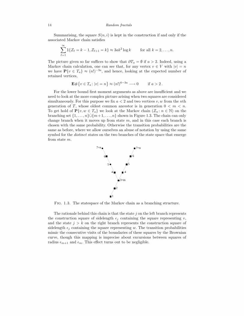
For the lower bound first moment arguments as above are insufficient and weneed to look at the more complex picture arising when two squares are consideredsimultaneously. For this purpose we fix a < 2 and two vertices v, w from the nthgeneration of T , whose oldest common ancestor is in generation 0 < m < n.To get hold of P{v, w ∈ Ta} we look at the Markov chain (Zn : n ∈ N) on thebranching set {1, . . . , n}∪{m+1, . . . , n} shown in Figure 1.3. The chain can onlychange branch when it moves up from state m, and in this case each branch ischosen with the same probability. Otherwise the transition probabilities are thesame as before, where we allow ourselves an abuse of notation by using the samesymbol for the distinct states on the two branches of the state space that emergefrom state m.

����

����

����

����

��

��

��

����

����

1

2

3=m

4

5

6

4

5

6

7=n 7=n

Fig. 1.3. The statespace of the Markov chain as a branching structure.

The rationale behind this chain is that the state j on the left branch representsthe construction square of sidelength εj containing the square representing v,and the state j > k on the right branch represents the construction square ofsidelength εj containing the square representing w. The transition probabilitiesmimic the consecutive visits of the boundaries of these squares by the Browniancurve, though this mapping is imprecise about excursions between squares ofradius εm+1 and εm. This effect turns out to be negligible.

Fine properties of stochastic processes 15

A Markov chain calculation shows that

P{

v, w ∈ Ta

}

≈ (n!)−6a (k!)3a ,

and from this we obtain a constant C > 0 and a bound on the variance

E[(

#{

v ∈ Ta : |v| = n})2] ≤ C E

[

#{

v ∈ Ta : |v| = n}]2

.

We can therefore use the Paley-Zygmund inequality to derive, for any 0 < λ < 1,

P{

#{

v ∈ Ta : |v| = n}

≥ (1 − λ)E[

#{

v ∈ Ta : |v| = n}]

}

≥ λ2 E[#{v ∈ Ta : |v| = n}]2E[(#{v ∈ Ta : |v| = n})2] ≥ C−1 λ2 > 0 .

Recall that, if a < 2, we have

E[

#{

v ∈ Ta : |v| = n}]

−→ ∞,

and hence this argument shows that ∂Ta 6= ∅ with positive probability. A self-similarity argument (not unlike the Galton-Watson zero-one law) shows that thismust therefore hold with probability one.

Let me emphasise the importance of the correct choice of the scales (εk) forthe success of the tree approximation. If the ratio εk−1/εk is chosen significantlysmaller, the excursion counts typically do not reflect the occupation times atall radii and centres; observe that we need the equivalence analogous to (1.4)simultaneously for all squares of sidelength εk, k ∈ {2, . . . , n}, so that a rigorousproof requires a much more quantitative approach to this part of the argumentthan our informal discussion suggests. Conversely, if the ratio εk−1/εk is chosensignificantly larger, we lose the necessary control over the occupation times forintermediate radii.

Finally, a note of caution: Turning this picture into a full proof of Theo-rem 1.11 still requires skill and a lot of work, as we oversimplified at many places.Nevertheless, the tree representation gives a neat organisation of the complicateddependencies, which greatly helps understanding and solving this hard problem.

1.2.2 The multifractal spectrum of intersection local time

The multifractal spectrum is an important means of describing the fine struc-ture of a fractal measure, see (Morters, 2008) for a subjective discussion of itsimportance in the context of stochastic processes. For a precise definition, fix alocally finite measure µ, which may be random or non-random. The value f(a)of the multifractal spectrum is the Hausdorff dimension of the set of points xwith local dimension

limr↓0

log µ(B(x, r))

log r= a, (1.5)

where B(x, r) denotes the open ball of radius r centred in x. In some cases ofinterest, the limit in (1.5) has to be replaced by liminf or limsup to obtain aninteresting nontrivial spectrum.

16 Random fractals

Examples of multifractal spectra for measures arising in probability are theoccupation measures of stable subordinators (Hu and Taylor, 1997), the states ofsuper-Brownian motion (Perkins and Taylor, 1998), and the harmonic measureon a Brownian path (Lawler, 1997). The example we study here has some likenesswith the first two examples, for which a similar tree analogy could be built,though details in the proof invariably differ considerably.

We look at two independent planar Brownian motions (W (1)

t : 0 ≤ t ≤ 1) and(W (2)

t : 0 ≤ t ≤ 1) and study the intersection set

S ={

x ∈ R2 : there exist 0 ≤ s, t ≤ 1 with W (1)

s = W (2)

t = x}

.

The natural measure on S is the intersection local time µ defined symbolically by

µ(A) =

∫

A

dx

2∏

i=1

∫ 1

0

ds δ0(W(i)

s − x) ,

Rigorous definitions of µ can be given by approximation of the ‘delta-function’ δ0,but also as a suitable Hausdorff measure on S. Technical details of the construc-tion are not of interest to us here.

Theorem 1.12 For every 2 ≤ a ≤ 7011 we have, almost surely,

dim{

x ∈ S : lim supr↓0

log µ(B(x, r))

log r= a

}

=1

12

(70

a− 11

)

.

Moreover, there are no points with local dimension a < 2 or a > 7011 in any

sense (liminf, limsup, or lim). At least heuristically, all the results concerningvalues a ≥ 2 can be read off a tree picture, which we describe below. The fullproof of the result, which is inspired by this tree picture but does not makeexplicit use of it, can be found in Klenke and Morters (2005).

As S is the intersection of two independent sets of full dimensions (the Brow-nian paths) it is not surprising that dimS = 2 and therefore µ(B(x, r)) ≈ r2 fortypical points x ∈ S. Fix a > 2 for the remainder of this section. For the pointsx ∈ S with

µ(B(x, r)) ≈ ra � r2

we expect that

• the ball B(x, r) is visited only once by each Brownian motion,

• the intersection local time spent in B(x, r) during this visit is small.

Due to the first item, the recurrence effects that were so crucial in the proof ofTheorem 1.11 do not play a role here. Indeed, here we can assume that for disjointballs B(x, r) and B(y, r) the events {µ(B(x, r)) ≈ ra} and {µ(B(y, r)) ≈ ra} areessentially independent. This simplifies the informal discussion immensely, butmaking this argument rigorous is one of the main difficulties in the proof ofTheorem 1.12, which we do not discuss here.

Fine properties of stochastic processes 17

The remainder of our discussion of this example is based on this independence(or locality) assumption. Fix a square S ⊂ R

2 of unit sidelength and pick a largeinteger m. Divide the square into m2 squares of sidelength 1/m, and keep asquare if it contains a point of S, then repeat this procedure with any squarekept, and so on at infinitum. Identifying the squares kept in the procedure withvertices in a tree T = (V, E), we obtain a tree representation of S ∩ S.

To connect the intersection local time µ to this tree representation, we recalla result of Le Gall (1986), which states that µ can be recovered from the volumeof the Wiener sausages around the two Brownian paths, more precisely

limε↓0

(log ε)2

π2vol

(

S(1)

ε ∩ S(2)

ε ∩ A)

= µ(A) ,

where S(i)ε = {x ∈ R

2 : |W (i)

t − x| ≤ ε for some 0 ≤ t ≤ 1}. This suggests that,given a square v ∈ V , we have that

µ(v) ≈ limn→∞

Zn(v)

m2nn−2,

where Zn(v) is the number of offspring of v in the nth generation. Note that themean number of children of a vertex in the nth generation is of order ≈ m2(n−1

n )2

and hence is generation dependent.

Instead of looking for a strong analogy and discussing generation dependentoffspring distributions, for this exposition we sacrifice precision in favour of sim-plicity and claim that in this analogous case the most interesting features of theoriginal problem are still present. More precisely, we look at a Galton-Watsontree such that every vertex has a mean number m2 of children, and discuss themultifractal spectrum of the branching measure µ on its boundary, defined by

µ(

B(v))

= limn→∞

Zn(v)

m2n,

where B(v) is the set of rays passing through the vertex v. Fixing some b > 1,we endow ∂T with the metric such that the distance of two rays is b−n, wheren is the generation of their last common ancestor. In this metric, the set B(v)is the ball centred in v of radius b−|v|, so that for the choice of b = m thiscorresponds to the sidelength and therefore, up to a constant, to the diameterof the represented square.

We state a general result for the multifractal spectrum of Galton-Watsontrees with generating variable N and finite mean, which is taken from Mortersand Shieh (2004).

Theorem 1.13 Suppose P{N = 0} = 0 and 0 < P{N = 1} < 1. Define

a = log EN > 0 and τ = − logP{N = 1}/ logEN > 0.

Then, for all a ≤ θ ≤ a(

1 + 1τ

)

, almost surely,

dim{

(v0, v1, . . .) ∈ ∂T : lim supn→∞

log µ(B(vn))

−n= θ

}

=a

log b

(a

θ(1 + τ) − τ

)

.

18 Random fractals

Before looking at the structure of this result in more detail, let us adaptthe parameters of our tree representation in good faith. We have already notedthat EN = m2 and by construction we have N ≥ 1 so that the conditions ofTheorem 1.13 are satisfied. For the metric we would like to choose b = m, andthe remaining parameter is P{N = 1}, which we write as m−η for some η > 0,which we discuss later. We obtain a = 2 logm, τ = η/2 and hence a predictedspectrum of

dim{

x ∈ S : lim supr↓0

log µ(B(x, r))

log r= θ

}

= 2(2

θ(1 +

η

2) − η

2

)

.

Note that neither side of this equation has any dependence on m, which gives usa handle on η, which we only have to determine asymptotically for m ↑ ∞.

To do this we require knowledge of a probability exponent, roughly defined asthe rate of decay (as r ↑ ∞) of the probability of an increasingly unlikely eventinvolving Brownian paths running until they exit the ball B(0, r). Various kindsof exponents can be defined and used in fractal geometry, see Lawler (1999).

In the present case we need an intersection exponent. To define these, supposek, m ≥ 1 are integers, and (W (i)

s : s ≥ 0) for i ∈ {1, . . . , k + m} are independentBrownian motions started on the unit sphere ∂B(0, 1), and stopped upon leavingB(0, en), i.e. at times T (i)

n = inf{s > 0: |W (i)s | = en}. We denote by

B(1)

n =

k⋃

i=1

{

W (i)

s : 0 ≤ s ≤ T (i)

n

}

,

B(2)

n =

k+m⋃

i=k+1

{

W (i)

s : 0 ≤ s ≤ T (i)

n

}

,

two packets of paths, and assume that the starting points in different packetsare different. Denote by Vn the event that the two packets B

(1)n and B

(2)n do not

intersect each other. The intersection exponents are defined by the requirementthat there exist constants 0 < c < C such that

c exp{−n ξ(k, m)} ≤ P(Vn) ≤ C exp{−n ξ(k, m)} .

Lawler (1996b) showed that the intersection exponents ξ(k, m) are well-definedby this requirement, and some years later the (highly nontrivial) techniques ofstochastic Loewner evolution (SLE) enabled Lawler, Schramm and Werner togive the explicit values

ξ(k, m) =(√

24k + 1 +√

24m + 1 − 2)2 − 4

48.

For a short survey of the key steps in this development and some other earlyapplications of the SLE technique, see (Lawler et al., 2001).

Fine properties of stochastic processes 19

Let us explain how intersection exponents help identifying P{N = 1} in ourtree model. Suppose S is any square containing an intersection point (hencecorresponding to a vertex in the tree). The event {N = 1} means that theBrownian paths intersect in one of the m2 congruent nonoverlapping subsquareswhich cover S, but nowhere else in S.

S

S’

Fig. 1.4. Paths realising the event {N = 1}, the initial parts of both pathsare dashed.

We now fix one f these subsquares, say S ′, and assume (without significantloss of generality, as in the previous section) that it is located sufficiently far awayfrom the boundary of S. We split both motions at the first time they hit ∂S ′

and apply time-reversal to the initial part of each motion. Though the reversedpart are strictly speaking not Brownian motions, they are sufficiently similar totreat them as such. Then we are faced with four Brownian motions started at∂S′, which we divide in two packets of two, with each packet consisting of the(time-reversed) first part and the (non-reversed) second part of the same originalmotion. We consider all motions up to the first time when they hit ∂S, which isat distance of order m times the typical distance of the starting points. Hence,applying Brownian scaling, we get

P{

paths do not intersect outside S ′}

≈ m−ξ(2,2).

As these events are disjoint for the m2 different squares S′ ⊂ S we can sum theprobabilities and obtain

P{

N = 1}

≈ m2−ξ(2,2) as m ↑ ∞.

20 Random fractals

Hence η = ξ(2, 2) − 2 and plugging this into the prediction yields

dim{

x ∈ S : lim supr↓0

log µ(B(x, r))

log r= θ

}

= 2ξ(2, 2)

θ+ 2 − ξ(2, 2) .

Using the known value ξ(2, 2) = 3512 of the intersection exponents gives the precise

formula claimed in Theorem 1.12.

As in the previous example, a note of caution is necessary: The tree analogyis very suitable to develop an intuition for the problem and guess the right mul-tifractal spectrum. However, in setting up the tree analogy, we have gone too farto prove Theorem 1.12 by justification of the steps undertaken in this simplifi-cation and it is preferable to start this proof from scratch. The original problemneeds serious treatment before some form of the claimed locality assumption canbe exploited, and it seems to be impossible to carry out the proof without usingthe full power of the strong Markov property of the two Brownian motions.

However, an inspection of the proof of Theorem 1.13 gives structural insight,which is directly applicable to the proof of Theorem 1.12. Indeed, given a vertex vwith |v| = n, the event

{

µ(B(v)) ≈ e−nθ}

is typically coming up when Zk(v) = 1 for k = nθ/ logEN , i.e. when the vertex vhas just one offspring for k generations. This fact can be translated directly intothe Brownian world. A point x ∈ S typically satisfies

lim supr↓0

log µ(B(x, r))

log r≈ a

if there exists a sequence rn ↓ 0 of radii such that

(

B(x, rn) \ B(x, ra/2n )

)

∩ S = ∅ .

The occurence of large empty annuli at selected radii is also key to the under-standing of the multifractal spectrum of super-Brownian motion (Perkins andTaylor, 1998). Hence, despite greatly oversimplifying the situation, the tree ap-proach gives valuable insight into the original problem, which can be exploiteddirectly in the proof.

1.2.3 Points of infinite multiplicity

In this section we turn our attention to an attractive unsolved problem. It isknown for a long time that planar Brownian motion has points of multiplicity p,for any positive integer p. Moreover, Dvoretzky et al. (1958) have shown that,almost surely, there exist points of uncountably infinite multiplicity, see (Le Gall,1992) or (Morters and Peres, 2008) for modern proofs. These arguments can alsobe used to show that the Hausdorff dimension of the set of points of uncountablyinfinite multiplicity is still two.

Fine properties of stochastic processes 21

How far can we go, before we see a reduction in the dimension? A natural wayis to count the number of excursions from a point. To be explicit, let (Ws : s ≥ 0)be a planar Brownian motion and fix x ∈ R

2 and ε > 0. Let S−1 = 0 and, for anyinteger j ≥ 0, let Tj = inf{s > Sj−1 : Ws = x} and Sj = inf{s > Tj : |Ws − x| ≥ε}. Then define

Nxε = max

{

j ≥ 0: Tj < ∞}

,

which is the number of excursions from x hitting ∂B(x, ε). Observe that Nxε = 0

for almost every point on the curve (with respect to the occupation time Tintroduced in Section 1.2.1) and that

limε↓0

Nxε = ∞ ⇐⇒ x has infinite multiplicity.

It is therefore a natural question to ask how rapidly Nxε can go to infinity when

ε ↓ 0. A partial answer is given in the following theorem of Bass et al. (1994).

Theorem 1.14

(a) Let 0 < a < 12 . Then, almost surely,

dim{

x ∈ R2 : lim

ε↓0

Nxε

log(1/ε)= a

}

≥ 2 − a .

(b) Let 0 < a < 2e. Then, almost surely,

dim{

x ∈ R2 : lim

ε↓0

Nxε

log(1/ε)= a

}

≤ 2 − a

e.

(c) Almost surely, for every x ∈ R2, we have

lim supε↓0

Nxε

log(1/ε)≤ 2e.

Note, for comparison, that for a linear Brownian motion, almost surely, forevery x ∈ R, we have

limε↓0

(4ε) Mxε = Lx

t ,

where Mxε is the number of excursions from x hitting {x− ε, x+ ε} before time t,

and Lxt is the local time at x, see e.g. (Morters and Peres, 2008).

The proof of parts (b) and (c) of Theorem 1.14 is fairly straightforward,though the statements are certainly not optimal. The delicate part is the lowerbound, given in (a). This argument is based on the construction of a local time,a nondegenerate measure on the set

{

x ∈ R2 : lim

ε↓0

Nxε

log(1/ε)= a

}

.

The restriction to values a < 1/2 is due to the use of L2-estimates and appearsto be of a technical nature. It is believed that the following conjecture is true.

22 Random fractals

Conjecture 1.1 Almost surely,

maxx∈R2

limε↓0

Nxε

log(1/ε)= 2.

Moreover, for any 0 < a < 2, almost surely,

dim{

x ∈ R2 : lim

ε↓0

Nxε

log(1/ε)= a

}

= 2 − a .

This is still an open problem. Hope for its solvability comes from the factthat one can represent the dependence structure of the random variables Nx

ε ina tree picture similar to the one indicated in Section 1.2.1. However, because theBrownian path is required to return exactly to a given point, this problem hasmuch less inherent continuity than the two previous ones, and therefore appearsto be much harder.

1.3 More on the planar Brownian path

We have seen in the second example of the previous section that in some cases,once the tree technique has been exploited, there remains a serious challenge toidentify the rate of decay of certain probabilities associated with the underlyingprocess. This challenge can be formalised in the notion of probability exponents,and in this section we give further evidence of their use in fractal geometry,following ideas surveyed in Lawler (1999).

1.3.1 The Mandelbrot conjecture

We look at a famous example, the Mandelbrot conjecture: Let (Ws : 0 ≤ s ≤1) be a planar Brownian motion running for one time unit and consider thecomplement of its path,

{

x ∈ R2 : x 6= Ws for any 0 ≤ s ≤ 1

}

.

This set is open and can be decomposed into connected components, exactly oneof which is unbounded. We denote this component by U and define its boundary∂U as the frontier of the Brownian path. The frontier can be seen as the set ofpoints on the Brownian path which are accessible from infinity and is thereforealso called the outer boundary of Brownian motion.

According to a frequently told legend, Mandelbrot, when presented with asimulation of the Brownian frontier, cast a brief glance at the picture and imme-diately identified its dimension as 4/3, see (Mandelbrot, 1982). However, a morerigorous confirmation of this conjecture took a long time. In the late ninetiesBishop et al. (1997) showed that the frontier has Hausdorff dimension strictlylarger than one, and about the same time Lawler (1996a) identified the Hausdorffdimension in terms of a disconnection exponent.

More on the planar Brownian path 23

The disconnection exponents ξ(k), k ∈ N, can be defined as follows: Suppose(W (i)

s : s ≥ 0) for i ∈ {1, . . . , k} are independent Brownian motions startedon the unit sphere ∂B(0, 1), and stopped upon leaving B(0, en), i.e. at timesT (i)

n = inf{s > 0: |W (i)s | = en}. We denote by

Bn =

k⋃

i=1

{

W (i)

s : 0 ≤ s ≤ T (i)

n

}

the union of the paths, and by Vn the event that Bn does not disconnect the ori-gin from infinity, i.e. the origin is in the unbounded connected component of thecomplement of Bn. The disconnection exponents are defined by the requirementthat there exist constants 0 < c < C such that

c exp{−n ξ(k)} ≤ P(Vn) ≤ C exp{−n ξ(k)} .

Lawler (1996a) showed that the disconnection exponents ξ(k) are well-defined bythis requirement, and —just as in the case of intersection exponents— Lawler,Schramm and Werner found the explicit values

ξ(k) =(√

24k + 1 − 1)2 − 4

48.

Note that this is in line with the intersection exponents as (formally, because ofour requirement that m be an integer)

limm↓0

ξ(k, m) = ξ(k),

and this corresponds to the observation that if Bn disconnects the origin frominfinity, no further independent packet (no matter how slim, i.e. how small m)started at the origin can reach ∂B(0, en) without intersecting Bn. This can bemade rigorous by extending the definition of intersection exponents to nonintegerarguments.

In Lawler (1996a) the dimension of the frontier was identified to be 2− ξ(2),so that Mandelbrot’s conjecture follows.

Theorem 1.15 Almost surely, the Hausdorff dimension of the frontier is

dim ∂U = 43 .

It is not hard to paint a tree picture that makes the connection of the dis-connection exponents and the frontier clear. This time we prefer to work in thetime domain and use the following striking result of Kaufman, for a proof seee.g. (Morters and Peres, 2008).

Lemma 1.16. (Kaufman’s lemma) Suppose d ≥ 3 and (Ws : s ∈ [0, 1]) is ad-dimensional Brownian motion. Then, almost surely, for every A ⊂ [0, 1],

dim{

Ws : s ∈ A}

= 2 dim A .

24 Random fractals

Note that the ‘dimension doubling’ rule holds simultaneously for all setsA ⊂ [0, 1] with a single exceptional set of probability zero. It can therefore beapplied to any random set A, which makes Kaufman’s lemma a powerful tool.

We now look at the decomposition of the unit interval [0, 1] into 2n nonover-lapping intervals of equal length. Any such interval [j2−n, (j+1)2−n] is associatedto a vertex in a representing tree T if the set

B(j)

n ={

Ws : 0 ≤ s ≤ j2−n or (j + 1)2−n ≤ s ≤ 1}

does not disconnect {Ws : j2−n ≤ s ≤ (j + 1)2−n}

from infinity. With the rulethat a vertex v is an offspring of w if the interval associated to v is contained inthat associated to w, this constitutes a tree representation of the set

I(T ) = {s ∈ [0, 1] : Ws ∈ ∂U}.

This representation does not make I(T ) a Galton-Watson fractal, but thefollowing lemma taken from (Lawler, 1999, Lemma 1 and 2) indicates how, in aspecial situation, the independence conditions of Theorem 1.4 can be weakened.

Lemma 1.17 Given a family of (not necessarily independent) zero-one valuedrandom variables

{

Y (j1, . . . , jn) : ji ∈ {0, 1}, n ∈ N}

,

we build a random fractal A iteratively. Let S0 = {[0, 1]} and, given a collectionSn of compact intervals of length 2−n, construct a collection Sn+1 by

• splitting each interval in Sn−1 into two nonoverlapping intervals of halfthe length,

• adding any interval thus constructed to the collection Sn if

Y (j1, . . . , jn) = 1,

where∑n

i=1 ji2−i is the left endpoint of the interval.

Define the random fractal as

A =

∞⋂

n=1

⋃

I∈Sn

I .

Then

(i) If

1∑

j1,...,jn=0

E

n∏

k=1

Y (j1, . . . , jk) ≤ C 2(1−α)n for some C > 0, then

dim A ≤ 1 − α almost surely.

More on the planar Brownian path 25

(ii) If, for some 0 < c < C < ∞ and ε > 0,

c 2−αn ≤ E

n∏

k=1

Y (j1, . . . , jk) ≤ C 2−αn for all ε ≤n

∑

i=1

ji2−i ≤ 1 − ε,

and

E

n∏

k=1

Y (j1, . . . , jk)Y (i1, . . . , ik) ≤ C 2−2αn(

n∑

i=1

(ii − ji)2−i

)−α

,

for all ε ≤ ∑n1 ji2

−i <∑n

1 ii2−i ≤ 1 − ε, then

dim A ≥ 1 − α with positive probability.

This lemma exploits a tree representation of A with the tree T given as asubtree of a binary tree with vertices in the nth generation canonically denotedby (j1, . . . , jn). Such a vertex is contained in T if and only if

n∏

k=1

Y (j1, . . . , jk) = 1 .

The set attached to the vertex (j1, . . . , jn) is the closed interval of length 2−n

with left endpoint∑n

1 ji2−i, and the number of children of this vertex is

Y (j1, . . . , jn, 0) + Y (j1, . . . , jn, 1) .

Supposing that all the random variables Y (j1, . . . , jk) are independent, we get

min{

s : E{

2−sY (j1, . . . , jn, 0) + 2−sY (j1, . . . , jn, 1)}

≤ 1}

= min{

s : 2−s−α+1 ≤ 1}

= 1 − α,

confirming that this generalises a special case of Theorem 1.4.

In our case, we let Y (j1, . . . , jn) = 1 if and only if the set{

Ws : 0 ≤ s ≤ ∑ni=1 ji2

−i or∑n

i=1 ji2−i + 2−n ≤ s ≤ 1

}

does not disconnect

{Ws :

n∑

i=1

ji2−i ≤ s ≤

n∑

i=1

ji2−i + 2−n

}

from infinity. Using Brownian scaling and the definition of the disconnectionexponents, one can show that the probability of this event is of order 2−n

2 ξ(2),and that the second condition in (ii) also holds. This argument therefore givesthat

dim{

s ∈ [0, 1] : Ws ∈ ∂U}

= 1− 12 ξ(2) = 2

3 ,

with positive probability, and an application of Kaufman’s lemma gives dim ∂U =43 with positive probability. Some nontrivial extra work is required to show thatthis actually holds with probability one.

26 Random fractals

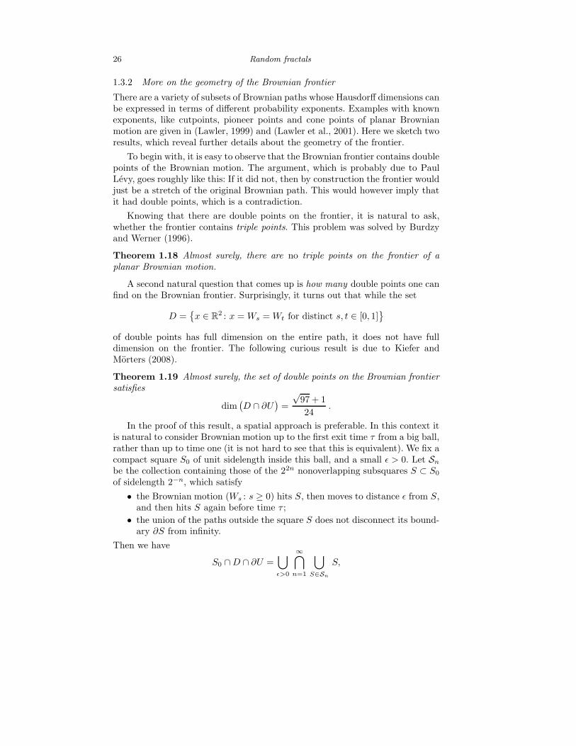
1.3.2 More on the geometry of the Brownian frontier

There are a variety of subsets of Brownian paths whose Hausdorff dimensions canbe expressed in terms of different probability exponents. Examples with knownexponents, like cutpoints, pioneer points and cone points of planar Brownianmotion are given in (Lawler, 1999) and (Lawler et al., 2001). Here we sketch tworesults, which reveal further details about the geometry of the frontier.

To begin with, it is easy to observe that the Brownian frontier contains doublepoints of the Brownian motion. The argument, which is probably due to PaulLevy, goes roughly like this: If it did not, then by construction the frontier wouldjust be a stretch of the original Brownian path. This would however imply thatit had double points, which is a contradiction.

Knowing that there are double points on the frontier, it is natural to ask,whether the frontier contains triple points. This problem was solved by Burdzyand Werner (1996).

Theorem 1.18 Almost surely, there are no triple points on the frontier of aplanar Brownian motion.

A second natural question that comes up is how many double points one canfind on the Brownian frontier. Surprisingly, it turns out that while the set

D ={

x ∈ R2 : x = Ws = Wt for distinct s, t ∈ [0, 1]

}

of double points has full dimension on the entire path, it does not have fulldimension on the frontier. The following curious result is due to Kiefer andMorters (2008).

Theorem 1.19 Almost surely, the set of double points on the Brownian frontiersatisfies

dim(

D ∩ ∂U)

=

√97 + 1

24.

In the proof of this result, a spatial approach is preferable. In this context itis natural to consider Brownian motion up to the first exit time τ from a big ball,rather than up to time one (it is not hard to see that this is equivalent). We fix acompact square S0 of unit sidelength inside this ball, and a small ε > 0. Let Sn

be the collection containing those of the 22n nonoverlapping subsquares S ⊂ S0

of sidelength 2−n, which satisfy

• the Brownian motion (Ws : s ≥ 0) hits S, then moves to distance ε from S,and then hits S again before time τ ;

• the union of the paths outside the square S does not disconnect its bound-ary ∂S from infinity.

Then we have

S0 ∩ D ∩ ∂U =⋃

ε>0

∞⋂

n=1

⋃

S∈Sn

S,

References 27

and the Hausdorff dimension can be determined (with positive probability) byverifying a first and second moment criterion analogous to (i), (ii) in Lemma 1.17.

For the first moment criterion, we have to show that the probability that acube of sidelength 2−n is in Sn is bounded from above and below by constantmultiples of 2−nξ(4). Indeed, we may use three stopping times to split the pathinto four pieces: They are the first hitting time of S, the first time afterwardswhere the path has moved to distance ε from the square, the first hitting timeof S after that. If we reverse the first and third part in time, the four pieces aresufficiently close to Brownian paths started on the boundary of the cube andrunning for one time unit, to infer that the probability of disconnection is, up toa factor which is polynomial in n, of order 2−nξ(4). At this place the proof is abit more delicate than the arguments in Section 1.2.2, because a careful controlof the polynomial factors is required.

This first moment argument, a slightly more sophisticated one for the secondmoment, and a tree framework similar to the one above, show that, with positiveprobability,

dim(

D ∩ ∂U)

= 2 − ξ(4) =

√97 + 1

24.

Again, some more work is required to show that this holds almost surely.

For Theorem 1.18 the argument is easier, as no lower bound is needed. Usingno more than the Borel-Cantelli lemma one can infer that for

T ={

x ∈ R2 : x = Wr = Ws = Wt for distinct r, s, t ∈ [0, 1]

}

we have T ∩ ∂U = ∅ almost surely, if ξ(6) > 2. The merit of the paper (Burdzyand Werner, 1996) is mostly in providing this estimate long before the SLE-technology allowed the precise calculation of this value.

Acknowledgement: I would like to thank Yuval Peres for teaching me the ‘tree’ pointof view, and Richard Kiefer for permission to include our (yet unpublished) result. Iwould also like to acknowledge the support of EPSRC through an Advanced ResearchFellowship.

References

Bass, R. F., K. Burdzy, and D. Khoshnevisan (1994). Intersection local timefor points of infinite multiplicity. Ann. Probab. 22 (2), 566–625.

Bishop, C. J., P. W. Jones, R. Pemantle, and Y. Peres (1997). The dimensionof the Brownian frontier is greater than 1. J. Funct. Anal. 143 (2), 309–336.

Burdzy, K. and W. Werner (1996). No triple point of planar Brownian motionis accessible. Ann. Probab. 24 (1), 125–147.

Dembo, A. (2005). Favorite points, cover times and fractals. In Ecole d’Ete deProbabilites de Saint-Flour XXXIII—2003, Volume 1869 of Lecture Notes inMath., pp. 1–101. Berlin: Springer.

28 Random fractals

Dembo, A., Y. Peres, J. Rosen, and O. Zeitouni (2001). Thick points for planarBrownian motion and the Erdos-Taylor conjecture on random walk. ActaMath. 186 (2), 239–270.

Dvoretzky, A., P. Erdos, and S. Kakutani (1958). Points of multiplicity c ofplane Brownian paths. Bull. Res. Council Israel Sect. F 7F, 175–180 (1958).

Falconer, K. (1986). Random fractals. Math. Proc. Cambridge Philos.Soc. 100 (3), 559–582.

Falconer, K. (2003). Fractal geometry (Second ed.). Hoboken, NJ: John Wiley& Sons Inc. Mathematical foundations and applications.

Ford, Jr., L. R. and D. R. Fulkerson (1962). Flows in networks. Princeton,N.J.: Princeton University Press.

Graf, S., R. D. Mauldin, and S. C. Williams (1988). The exact Hausdorff di-mension in random recursive constructions. Mem. Amer. Math. Soc. 71 (381).

Hausdorff, F. (1918). Dimension und außeres Maß. Math. Ann. 79 (1-2), 157–179.

Hu, X. and S. J. Taylor (1997). The multifractal structure of stable occupationmeasure. Stochastic Process. Appl. 66 (2), 283–299.

Kiefer, R. and P. Morters (2008). Hausdorff dimension of the set of doublepoints on the Brownian frontier. In preparation.

Klenke, A. and P. Morters (2005). The multifractal spectrum of Brownianintersection local times. Ann. Probab. 33 (4), 1255–1301.

Lawler, G. (1996a). The dimension of the frontier of planar Brownian motion.Electron. Comm. Probab. 1, Paper 5, 29–47.

Lawler, G. (1996b). Hausdorff dimension of cut points for brownian motion.Electron. Journal Probab. 1, Paper 2, 1–20.

Lawler, G. (1997). The frontier of a Brownian path is multifractal. Unpublishedmanuscript , 24pp.

Lawler, G. (1999). Geometric and fractal properties of Brownian motion andrandom walk paths in two and three dimensions. Bolyai Society MathematicalStudies 9, 219 – 258.

Lawler, G. F., O. Schramm, and W. Werner (2001). The dimension of theplanar Brownian frontier is 4/3. Math. Res. Lett. 8 (4), 401–411.

Le Gall, J.-F. (1986). Sur la saucisse de Wiener et les points multiples dumouvement brownien. Ann. Probab. 14 (4), 1219–1244.

Le Gall, J.-F. (1992). Some properties of planar Brownian motion. In Ecoled’Ete de Probabilites de Saint-Flour XX—1990, Volume 1527 of Lecture Notesin Math., pp. 111–235. Berlin: Springer.

Lyons, R. and Y. Peres (2008). Probability on trees and networks. Cambridge:Cambridge University Press. Forthcoming.

Mandelbrot, B. B. (1982). The fractal geometry of nature. San Francisco,California: W. H. Freeman and Co.

Mauldin, R. D. and S. C. Williams (1986). Random recursive construc-tions: asymptotic geometric and topological properties. Trans. Amer. Math.Soc. 295 (1), 325–346.

References 29

Morters, P. (2008). Why study multifractal spectra? In Trends in Stochas-tic Analysis: A Festschrift in Honour of Heinrich v. Weizsacker, Volume 353of London Mathematical Society Lecture Note Series. Cambridge: CambridgeUniversity Press.

Morters, P. and Y. Peres (2008). Brownian motion. Cambridge: CambridgeUniversity Press. Forthcoming.

Morters, P. and N.-R. Shieh (2004). On the multifractal spectrum of a Galton-Watson tree. J. Appl. Prob. 41, 1223 –1229.

Perkins, E. A. and S. J. Taylor (1998). The multifractal structure of super-Brownian motion. Ann. Inst. H. Poincare Probab. Statist. 34 (1), 97–138.

Taylor, S. J. (1986). The measure theory of random fractals. Math. Proc.Cambridge Philos. Soc. 100 (3), 383–406.