Page 1
fz-
RANDOM
.
INSERTION INTO A PRI OR ITY QUEUE STRUCTURE
Thomas Porter
Istvan Simon
STAN-C S-74-460
OCTOBER 1974
COMPUTER SC IENCE DEPARTMENT
School of Humanities and SciencesSTANFORD UN IVERS ITY
Page 3
Random Insertion into a Priority Queue Structure
bY
Thomas Porter
Istvan Simon*J
Abstract
The average number of levels that a new element moves up when
' inserted into a heap is investigated. Two probabilistic models, under
which such an average might be computed are proposed. A "lemma of
conservation of ignorance" is formulated and used in the derivation of
an exact formula for the average in one of these models. It is shown
that this average is bounded by a constant and its asymptotic behavior
is discussed. Numerical data for the second model is also provided and
analyzed.
Keywords and phrases: Priority queue, heap insertion, heap sort,
analysis of algorithms.
CR Categories: 5.25, 5.31
J*On leave of absence from the Instituto de Matematica e Estatisticada Universidade de S"ao Paulo, depto. de Matematica Aplicada.
This research was supported in part by the National Science Foundationgrant number GJ 36473~ and by the FundacBo de Amparo a Pesquisa doE&ado de S&o Paul0 under grant number 72/425. Reproduction in wholeor in part is permitted for any purpose of the United States Government.
1
Page 4
Random Insertion into a Priority Queue Structure
1. Introduction
In this paper we investigate the average number of levels that a
new element moves up when inserted into an (n-l) -heap to form an
n-heap. An n-heap [Williams - 1964, Knuth - 19731 is a complete
binary tree of n nodes such that the key associated with each node
. is larger than the keys of both of its sons. Given an (n-l) -heap,
a new node can be inserted by placing it initially at the bottom of
the tree, thereby creating a complete binary tree of n nodes, and
then repeatedly comparing the key of the inserted node, x , with the
key of its father, y , exchanging the two nodes if x > y . If at
any stage x < y the resulting binary tree is an n-heap. Since a
complete binary tree of n nodes has Llg(n)J+l levels, -I* the
inserted node moves up at most Llg(n)J levels. Hence we can create
an n-heap by repeated application of this process in less than nL& nJ
operations. This suggests that the heap insertion method just described
could be used in the heap creation phase of heapsort [Knuth - 1973,
Section 5.2.3, Algorithm H]. One might expect that the average behavior
of the heap insertion method is still much better. Actually Williamsr
INHEAP routine in his original paper is essentially the insertion method
just described, and he states without proof in the comment accompanying
his routine that the average number of exchanges is two. In one of the
models proposed in this paper we shall prove that the average is bounded
by a constant less than two.
*J lg n denotes log2 n .
Page 5
To avoid ambiguities we state now the precise description of the
insertion algorithm. In this description we make use of the well known
compact representation of a complete binary tree in an array k ,
where k[l] is the root, and k[j] has left son k[2j] and right
son k[2j+l] . We also assume that each node consists only of its key.
If there are other fields of the node besides the key, the corresponding
modification of Algorithm I is trivial, and it obviously has no effect
on the average we are investigating here.
m. This algorithm inserts the n-th node into a heap. The
heap is stored in k[l],k[2],..., k[n-l] and k[n] is the node to be
inserted.
2. [Initialize.] Set p + n , q + p/2,1 , k + k[n] .
&2&- [Sift it up.] While q >O and k[q] < k do
end.begin HP] - khl 9 P + q 9 q + LP/~J
2. [Insert.] Set k[p] + k .
2. The Models
0
Let H(n) denote the number of n-heaps with n given distinct
keys, kl,k2, l vk, l The following closed form is known [Knuth - 1973,
Section 5.231 for H(n) :
H(n) n!
lT S.lLi<n i-
I (1)
where si is the size of the sub-tree rooted at node k[i] .
3
Page 6
Definition: Let A(n) denote the average number of levels the n-th
node is moved up by Algorithm I.
To find A(n) we consider two models:
Model 1: We assume that each of the H(n-1) possible heaps with the
(n-1) elements already in the heap☯klh2, b l vknmll
is equally likely,
and that the key of the n-th node kn is equally likely to occur in any
of the n intervals determined by kl,k2,...,kn 1 . In Section 4 we
shall derive a simple recursive formula for e-4 in this case.
Furthermore, we shall prove several properties of this formula in
Section 5.
The assumption that each of the H(n-1) possible heaps is equally
likely is justified if one uses the heap creation algorithm of heapsort
[muth -19'i'% Section 5=2.3, Algorithm, H, heap creation phase] to build
the (n-l) -heap and then applies Algorithm I to insert the last element.
It is shown [Knuth -193, Section 5.2.3, Theorem H] that each (n-l) -heap
occurs with equal probability in this case. One could hope that a
similar theorem would hold for heap creation by repeated application of
Algorithm I. Unfortunately, this is not so, for certain heaps will
occur more-often than others if-we apply Algorithm I successively to a
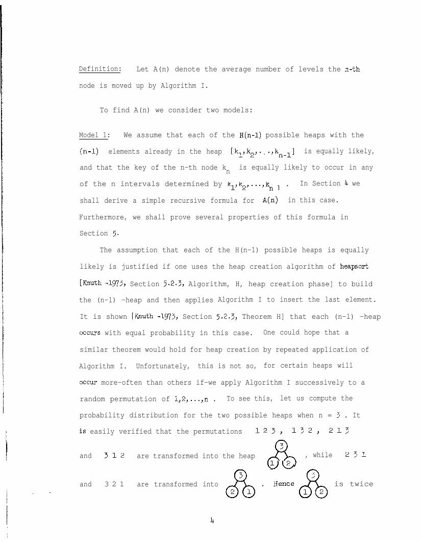
random permutation of 1,2,...,n . To see this, let us compute the
probability distribution for the two possible heaps when n = 3 . It
-is easily verified that the permutations 123, 132, 213
3and 312 are transformed into the heap
c%
, while 231
and 3 2 1 are transformed into & . lJ?Ief, & is twice
4
Page 7
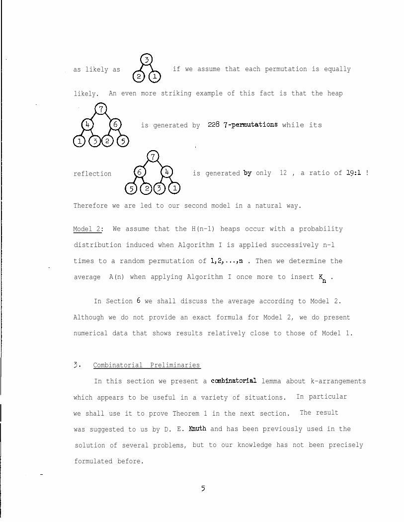
as likely as if we assume that each permutation is equally
likely. An even more striking example of this fact is that the heap
is generated by 228 7-permutations while its.reflection is generated bY only 12 , a ratio of 1g:l !
Therefore we are led to our second model in a natural way.
Model 2: We assume that the H(n-1) heaps occur with a probability
distribution induced when Algorithm I is applied successively n-l
times to a random permutation of 1,2,...,n . Then we determine the
average A(n) when applying Algorithm I once more to insert Kn .
In Section 6 we shall discuss the average according to Model 2.
Although we do not provide an exact formula for Model 2, we do present
numerical data that shows results relatively close to those of Model 1.
3. Combinatorial Preliminaries
In this section we present a cmbinatorial lemma about k-arrangements
which appears to be useful in a variety of situations. In particular
we shall use it to prove Theorem 1 in the next section. The result
was suggested to us by D. E. Knuth and has been previously used in the
solution of several problems, but to our knowledge has not been precisely
formulated before.
5
Page 8
Throughout this section, n and k denote fixed positive
integers with n > k .-
Definition:
(1) A k-arrangement of n objects is an ordered k-tuple of these
objects. A k-arrangement of k objects is called a k-permutation.
We shall consider only k-arrangements of {1,2,...,n) .
(2) Let CT be the set of k-arrangements of {1,2,...,n3 and let II
be the set of k-permutations of {1,2,...,k] . The function
f:a-Vt such that f((al,...,ak)) = (b1' l l
.,bk) implies
ai <a.J
= bi'b.3
is called the renumbering function preserving relative order. It
is obvious that for each n and k the renumbering function f
preserving relative order is unique.
3) A property P of k-arrangements is said to depend only on the
relative order of its elements when P(a) +S P(f(a)) for all
aa . (Note that since II c CT ,- f(a) ECT and hence we can talk
about P applied to f(a) 4
Examples:
(1) The property that the first element of the k-arrangement is the
largest one is a property that depends only on the relative order
of its elements.
(2) The property that the first k-l elements of the k-arrangement
form a (k-l) -heap is also such a property.
6
Page 9
Definition: A random variable over a certain space with uniform
probability distribution will be called simply a random variable over
that space.
We observe that the renumbering function f induces a partition
over the set CT , where two k-arrangements belong to the same equivalence
class, if and only if they are both mapped into the same k-permutation
by f l
*Lemmalz -I Let P be a property of k-arrangements that depends only
on the relative order of its elements. A random k-arrangement of
Cl 2Y f l �9 4satisfying P remains randam under the renumbering
function f preserving relative order.
Proof: All we have to prove is that an equal number of k-arrangements
that satisfy P are mapped by f into each k-permutation that
satisfies P l Notice that since P depends only on the relative
order of the elements of the k-arrangements, those that satisf'y P
are always mapped into k-permutations that satisfy P . l%rthermore,
if any k-arrangement of an equivalence class satisfies P , then all
k-arrangements of that class satisfy P . Hence we may simply show
that each equivalence class hasthe same number of elements. But there
are exactly k! equivalence classes each corresponding to a k-permutation.
Now consider any k-subset of {1,2,...,n) . Permuting its elements in
-
every possible order, it follows immediately from the definition of f
that exactly one of these k! permutations falls into each equivalence
*-/ L. Guibas has suggested that this lemma be named a "Principle of
Conservation of Ignorance", because the randomness is preservedthrough the renumbering process.
Page 10
class. Thus, since there are (E) k-subsets of Cl 2Y ,-**, 4 J there
are exactly (nk, elements in each equivalence class. ill
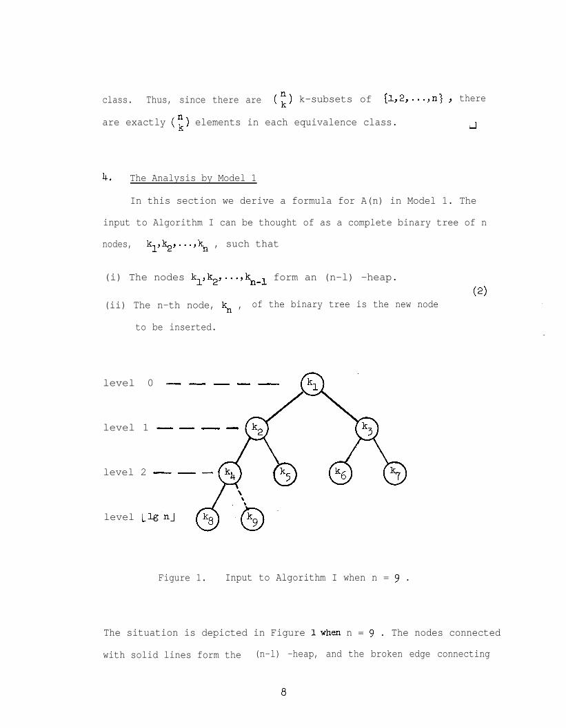
4. The Analysis by Model 1
In this section we derive a formula for A(n) in Model 1. The
input to Algorithm I can be thought of as a complete binary tree of n
nodes, kl,k2,...,kn , such that
(i) The nodes kl,k2,...,knml form an (n-l) -heap.
(2)(ii) The n-th node, kn , of the binary tree is the new node
to be inserted.
level 0 - - - - -
level 1 - - - -
level 2 - - -
level Llg-nJ
Figure 1. Input to Algorithm I when n = 9 .
The situation is depicted in Figure lwhen n = 9 . The nodes connected
with solid lines form the (n-l) -heap, and the broken edge connecting
8
Page 11
kYto the tree is used to indicate that k
9is the node to be inserted
into the heap. Thus, at this pointk9
is the only node that might
violate the heap condition key(son) < key(father) . It is important
to notice that as long as the relative order of kl,k2,...,k9
is
preserved, the values of the keys themselves are irrelevant as far as
the complexity of Algorithm I is concerned for this input. In other
words, Algorithm I will execute exactly the same sequence of instructions
for two inputs kl,k2, . . ..k. and ki,k;, . . ..kn satisfying condition (2),
, provided that their relative order is the same. Therefore we may as well
assume that
[kl,k2,~..,kn] = {1,2,...,n] = Mn . (3)
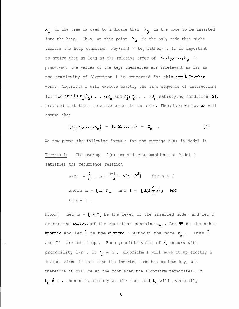
We now prove the following formula for the average A(n) in Model 1:
Theorem 1: The average A(n) under the assumptions of Model 1
satisfies the recurrence relation
n-lA(n) = i . L + 7 l A(n-2l) for n > 2
where L = Llg n] and 1 =
A(1) = 0 .
Proof: Let L = Llg-n] be the level of the inserted node, and let T
denote the subtree of the root that contains kn . Let T' be the other
subtree and let T be the subtree T without the node kn . Thus $
and T' are both heaps. Each possible value of kn occurs with
probability l/n . If kn = n , Algorithm I will move it up exactly L
levels, since in this case the inserted node has maximum key, and
therefore it will be at the root when the algorithm terminates. If
- kn+ny then n is already at the root and kn will eventually
9
Page 12
settle at some level in T . Therefore we may write
A(n) = i l L+G A[T] (4)
where A[T] denotes the average number of levels knis moved up in
the subtree T . The subtree T has exactly n-2' nodes, where
a = Llg($ n)] . (Note that 1 = L-l if T is the left subtree of
the root and 1 = L if it is the right one.)
Our aim now is to show that
A[T] = A(n-2l) . _ (5)
Fixing a particular T and varying the possible heap arrangements of
the nodes of T' we see that each T occurs exactly H(2!-1) times
among the original (n-l) -heaps, which are assumed equally likely by
hypothesis. Therefore each possible T is equally likely and we can
compute A[T] over the space of possible T-s . Keeping also in mind
that kn will eventually settle at some level in T , since kn e"n-1
and n is already at the root, this means that everything works as if
we were inserting kn into T rather than into the original (n-l) -heap.
Let US therefore assume from now on that our input is T . The input T
has k = n-2l nodes chosen from Mn 1 , and it can be regarded as a
k-arrangement of (1,2,:.. ,n-l')- such that its first (k-1) elements
form a heap. As we have seen before, this is a property of k-arrangements
that depends only on the relative order of its elements, and hence a
-random T remains random under the renumbering function f preserving
relative order, by Lemma 1. Furthermore by observation (3) above, the
renumbering process preserving relative order does not change the number
of levels that the inserted node is moved up by Algorithm I. Hence we
10
Page 13
can compute the average A[T] over the space of the renumbered trees.
But this is precisely A(n -2l) .Ll
50 Some Properties of the Average A(n)
In this section we shall explore some of the properties of the
average A(n) derived in Section 4. In particular we shall show that
at any level L of the tree the leftmost node, 2L , has the largest
We then proceed to prove-thatL
average. A(2 ) is always bounded by a
constant and approaches this constant as L approaches infinity, thus
showing that A(n) is bounded by a constant for all n . We then
derive a closed formula for n of the form 2wl-l , which is the
rightmost node at level L , and show that actually in this case a-4
is bounded by 1 and approaches 1 as L approaches infinity.
Finally we examine the asymptotic behavior of A(n) , where n varies
along an arbitrary path of the tree.
Theorem 2: If nl and n2 are two nodes at the same level L such
that nl is to the left of n2 (i.e., nl<n2 ), and if
Aby - 25
).l2
2 A(n2 -2 -) where Pi = L'g($"i)l Y then A(nl) > A ( >n2 l
Proof: By Theorem 1,
a.A(ni) = $- + (1 - 1)A(ni-2 i) l
i i
Since A(nl -25
1 2 Nn2-2I2
> Y
Page 14
Nq - Ah21
= (L-A(n2-2I2 )) .
Now L -A(n2 - 2l2
) > 0 , because (n2 - 2l2
) is a node at level
L-l , and it can move up at most L-l levels. It follows that
Nq > Ah21 l
Ill
Corollary 1: At each level L the leftmost node 2L has the largest
average value.
Proof: The proof is by induction. At level 0 the result is trivial.
Now assume the corollary at level L-l . Let nl be the leftmost
node at level L , and let n2 be a node to its right at the same
level. Then n2-2I2
is some node at level L-l , and nl-25 is
the leftmost node at that level (since fl = Llg( 5 n,)J = Llg($ 2L)J = L-l,
and5n -l2 = 2L-1 ). Therefore A(nl-25) > A(n2 -2 I2 ) by the
induction hypothesis, and the corollary follows from Theorem 2.0
We now examine the average at the leftmost nodes at each level.
aSince A(n) = A(n - 2’) + ’ OAF - 2 ) it follows that A(n) > A(n -2l)
for all n . In particular if n is the leftmost node, i.e., n = 2L ,
then n-2l = p Y henceL
A(2 ) is a monotonically increasing sequence
with L . It is not difficult to show that this sequence has a limit h ,
and hence it is bounded by this limit. By virtue of Corollary 1 this
I2
Page 15
implies that A(n) < h for all n , i.e., h is a constant that
bounds A(n) . Furthermore h is the best conceivable such bound
since lim A(2L) = h .L+a
We shall now determine a closed formula for LA(2 ) and use it to
derive an expression convenient for the numerical computation of h .
Theorem 3: The bound h satisfies the equalities
h = lim A(2L) = c -& = 1.6066951524 . . .L4a j>l 2J-l
Proof: We have A(2L) = L + (l-2-L)A(2L-1) by Theorem 1.eL
.
Let aL
denote A(2L) and let bL =aL
n (l-2-j) l
Then
l_<j<L
"L 2L= L + (l-2-L)aL-l and
T a, 1n y1-2-9 = $J
L + JJ’ln (1-2-j) n (1-2-j) ,
l_<jLL lsj_<L lsj<L-1-
i.e.,
bL = 2L. Lq- &-j)
+ bL-l l
(6)
Iterating equation (6) we get
cbL = bO+ l<i<L 2i
i
- - n (1-2-j) l
(7)
l<j<i-
13
Page 16
But b. = a0 = 0 , hence (7) yields
i n (l-2-j)l_<j_<L
&L =c
1LiLL gi jJ- (1-2-j) l
l:jLi
Let P = n (l-2-j) and Pj_>l
i= TTl_<j_<i
infinity, aL approaches h , hence
h=PC i
i>l 2i.
-
( 1-2-j) . If L approaches
(8)
(9)
By E'ulerrs partition formula [Knuth - 193, exercise 5.1.1-161,
Tr 1 i- c
Z 1
j>O (1-qjz) - _ TT @-CA.
i >0Setting z = z x and
llj,<i
1q=F=2
-1yields
R(x) = J--r 1
j>l l-2-jx=1+x _xi .
i>l 2%i
.
Let rj(x) = ' . . Then r;(x) = $ rj(x) =2-j
l-2-Jx - (l-2-jx)2 l
Taking derivatives of (10) and noting that R,(x) = ddx(j$ 'jcx') =
1 i-lwe have R'(x) = R(x) l c
jll 2j(l-2-jx)=x Lg..-.ill 2iP
i
In particular for x = 1 , noting that R(l) =--i , we have
14
Page 17
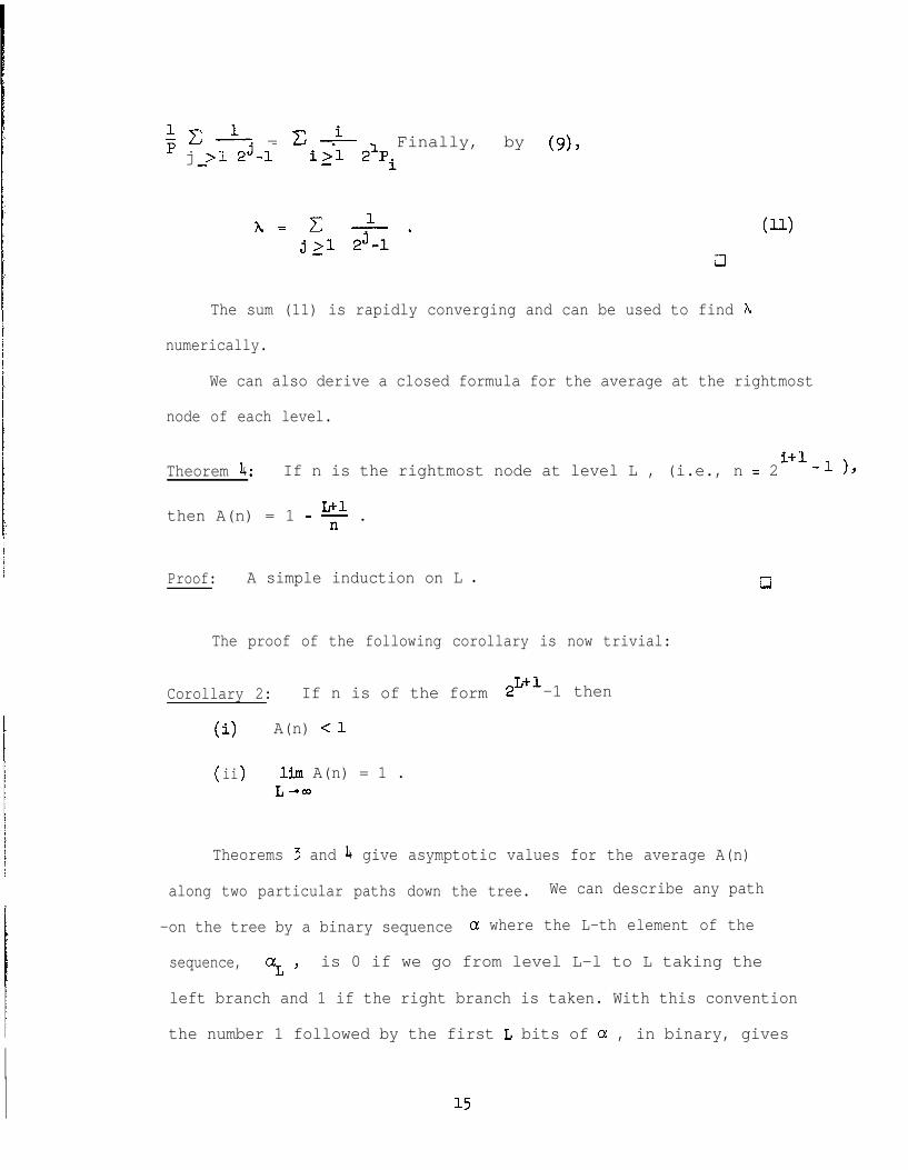
$ c 1 = c & g Finally, by (g),j >1 2j-1- i>l 2iPi-
A=c; -A.jzl 2J-l
u-ucl
The sum (11) is rapidly converging and can be used to find h
numerically.
We can also derive a closed formula for the average at the rightmost
node of each level.
Theorem 4: If n is the rightmost node at level L , (i.e., n = 2i+l-l ),
then A(n) = 1 - y .
Proof: A simple induction on L l
The proof of the following corollary is now trivial:
Corollary 2: If n is of the form2L+1-1 then
A(n) <l
0
( >ii lim A(n) = 1 .L-)a
Theorems 3 and 4 give asymptotic values for the average A(n)
along two particular paths down the tree. We can describe any path
-on the tree by a binary sequence Q where the L-th element of the
sequence, ?L Y is 0 if we go from level L-l to L taking the
left branch and 1 if the right branch is taken. With this convention
the number 1 followed by the first I, bits of a , in binary, gives
15
Page 18
the node at level L along that path. We denote this node by 2Lea .*J
Hence the limit A(a) = lim A(2L~~) , if it exists, gives the
asymptotic value of the average along the path defined by cx . If
the limit does not exist we say that A(a) is undefined. For example
a(0) = 000 . . . refers to the path of leftmost nodes at each level,
and thus A@(0)) = A according to Theorem 3, while a(1) = 111 . . .
refers to the path of rightmost nodes at each level, and thus
A(&)) = 1 by Corollary 2.
Definition:
(1) Two binary sequences a and p have the same tail if there exists
ani and j such that CX+~ = &3+k
for all k 2 0 .
(2) If m = n-2L , where I = Llg($ n)] then we say that the average
at node n depends on the average at node m .
This definition is motivated by Theorem 1.
Theorem 5: If Q! and @ are two binary sequences that have the
same tail, then A(a) and A(p) are either both undefined or both
defined and equal.
*J This notation is motivated by regarding a as associated with the
real number & = l+ c 0% LL l
Then the node denoted by 2 l a isL>l 2
clearly the node Note however that this correspondence
between a and & is not l-l , for sequences that are of the form
ala2 . . . aklOOO... and ala2 . ..a.rOlll... correspond to the
same real while defining distinct paths on the tree.
16
Page 19
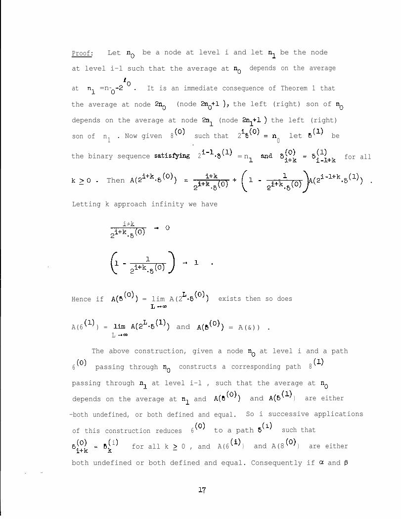
Proof: Let no be a node at level i and let nl be the node
at level i-l such that the average at no depends on the average
at fOnl
=n- .O2
It is an immediate consequence of Theorem 1 that
the average at node 2n0 (node 2no+1 ), the left (right) son of no
depends on the average at node 2nl (node 2nl+l ) the left (right)
son of n (0)1
. Now given 8 such that 2 6i (0) = n let 6 (1) be0L *
the binary sequence satiseing 2i+fjw = n (0)1 and 8. 6 (1)l+k= -i l+k for all
k>O. Then A(2i+k~6 (0) ) =- 1 - ,-g&q A(2i-l+k#)) .>
Letting k approach infinity we have
i+kp-J5y"
Hence if A(S (0) ) = lim A(2 08L (0)) exists then so doesL-)a
A(6 (1) ) = lim A(2L.s(1)) and A@(') ) = A(&)) .L 403
The above construction, given a node no at level i and a path
6 (0) passing through no constructs a corresponding path 8 (1)
passing through nl at level i-l , such that the average at no
depends on the average at n1 and A($ (0) ) and A@ (1) ) are either
-both undefined, or both defined and equal. So i successive applications.
of this construction reduces 6 (0) to a path 6 i( > such that
6 (0)i+k =
( >'k
i for all k 2 0 , and A(6 0) ) and A(8 (0) ) are either
both undefined or both defined and equal. Consequently if cx and 8
17
Page 20
have the same tail
path 6 such that
and A@) Y A(a)
and equal.
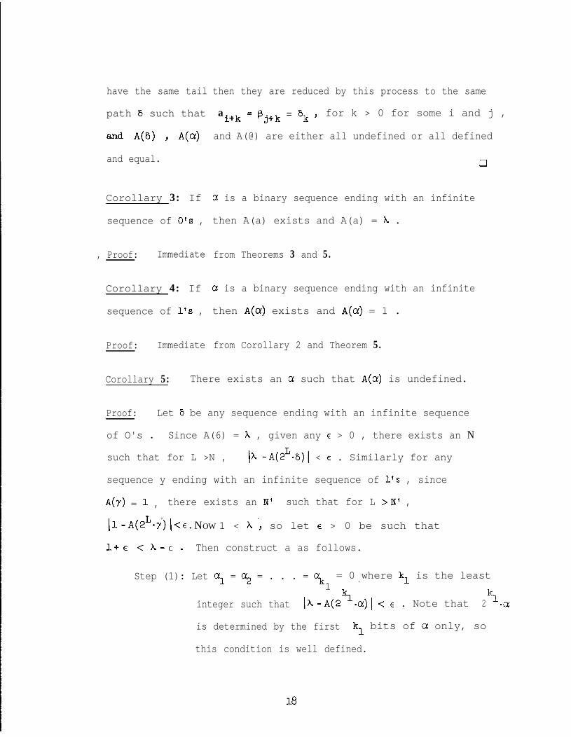
Corollary 3: If
sequence of 0's ,
, Proof: Immediate from Theorems 3 and 5.
Corollary 4: If
sequence of 193 , then A(a) exists and A(a) = 1 .
Proof: Immediate from Corollary 2 and Theorem 5.
then they are reduced by this process to the same
ai+k = Bj+k = 6k t for k > 0 for some i and j ,
and A(@) are either all undefined or all defined
cl
a is a binary sequence ending with an infinite
then A(a) exists and A(a) = h .
a is a binary sequence ending with an infinite
Corollary 5: There exists an a such that A@) is undefined.
Proof: Let 6 be any sequence ending with an infinite sequence
of O's . Since A(6) = )I , given any E > 0 , there exists an N
such that for L >N , \A -A(2L=S)I < E . Similarly for any
sequence y ending with an infinite sequence of l's , since
A(Y) = 1 , there exists an N, such that for L >N, ,
11-A(2L*r)( < E l NOW 1 < h, so let E > 0 be such that
l+e <k-E. Then construct a as follows.
Step (1): Let al = a2 = . . . = 5 = 0 where kl is the least1 '
integer such that lh-A(2kl .a)1 < e . Note that 2kl .a
is determined by the first kl bits of cx only, so
this condition is well defined.
18
Page 21
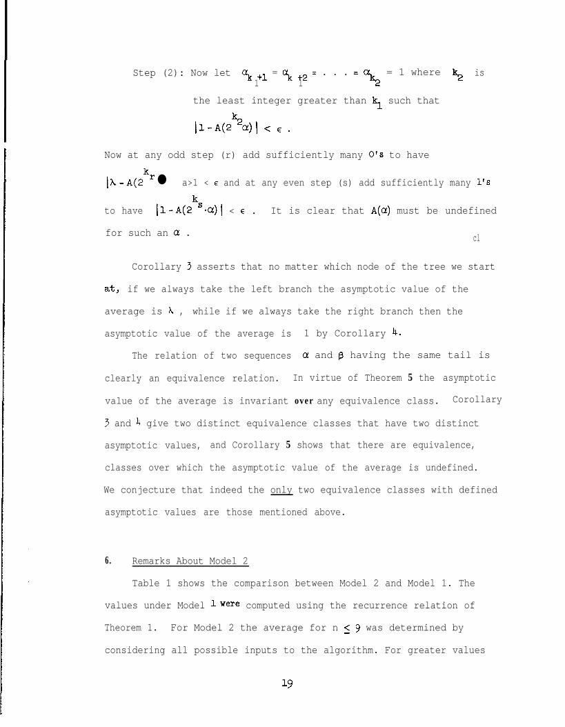
Step (2): Now let ~52 +1 = ak +2 = . . . = = 1 wherek2 is
1 1
the least integer greater than kl such that
ll-A(2k2a)\ < E .
Now at any odd step (r) add sufficiently many O's to have
(h_A(2krl a>1 < E and at any even step (s) add sufficiently many l's
to have ll-A(2kS41 < E . It is clear that A(a) must be undefined
for such an a . cl
Corollary 3 asserts that no matter which node of the tree we start
at, if we always take the left branch the asymptotic value of the
average is h , while if we always take the right branch then the
asymptotic value of the average is 1 by Corollary 4.
The relation of two sequences a and @ having the same tail is
clearly an equivalence relation. In virtue of Theorem 5 the asymptotic
value of the average is invariant over any equivalence class. Corollary
3 and 4 give two distinct equivalence classes that have two distinct
asymptotic values, and Corollary 5 shows that there are equivalence,
classes over which the asymptotic value of the average is undefined.
We conjecture that indeed the only two equivalence classes with defined
asymptotic values are those mentioned above.
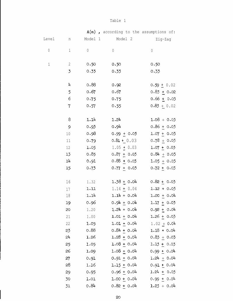
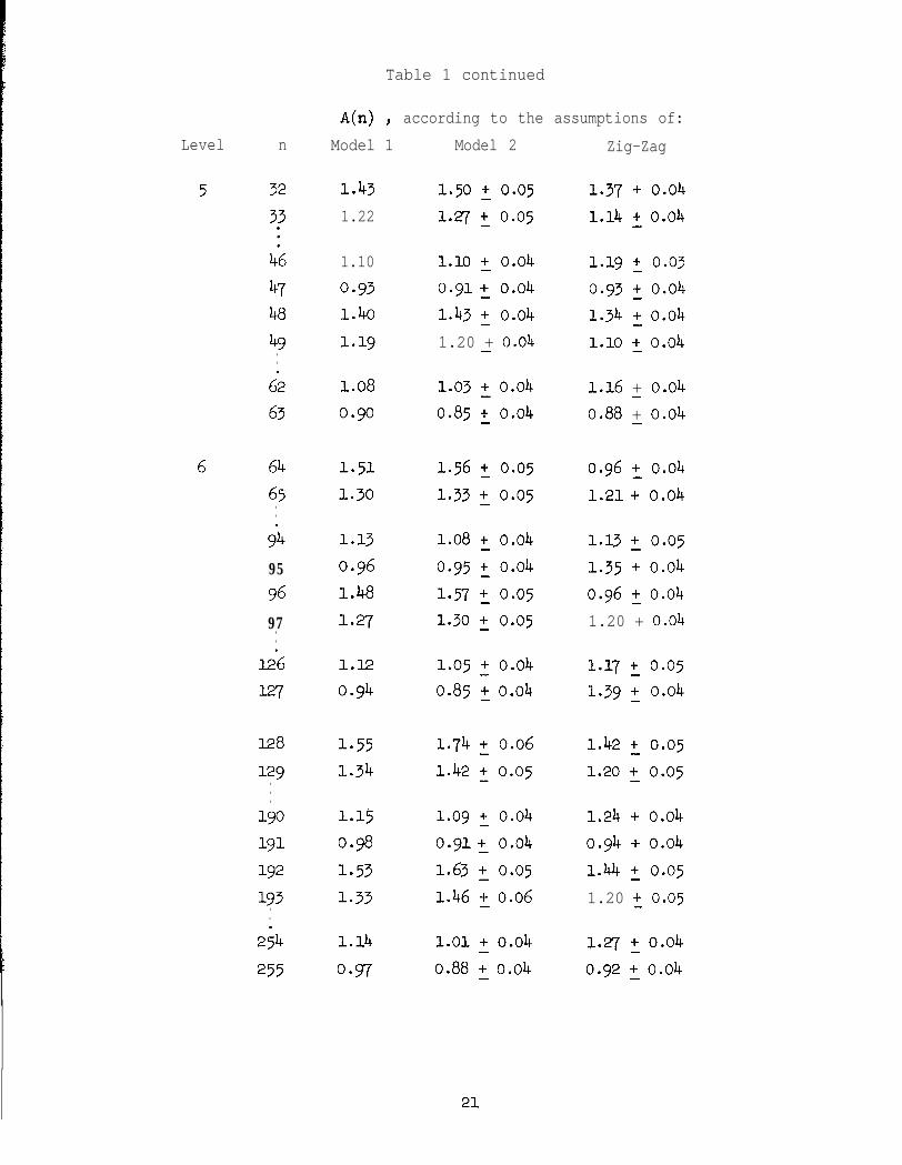
6. Remarks About Model 2
Table 1 shows the comparison between Model 2 and Model 1. The
values under Model lwere computed using the recurrence relation of
Theorem 1. For Model 2 the average for n ,< 9 was determined by
considering all possible inputs to the algorithm. For greater values
19
Page 22
Table 1
a-4 Y according to the assumptions of:
Level n
0 1
1 2
3
Model 1 Model 2 Zig-Zag
0 0
0.50
0.33
0.50
0.33
4 0.88 0.92
5 0.67 0.67
6 o-75 o-75
7 0.57 o-55
8 1.14
9 0.93
10 0.98
11 o-7912 1.05
13 0.85
14 0.91
15 o-73
1.24
0.94
0.99 + 0.03
0.81+ 0.03-1.05 + 0.03
0.87 + 0.03
0.88 + 0.03-0.77 + 0.03
16 1.32
17 1.11
18 1.14
19 0.96
20 1.20
21 1.00
22 1.05
23 0.88
24 1.26
25 1.05
26 1.09
27 0.91
28 1.16
29 0.95
30 1.01
31 0.84
1.38 + 0.04-1.14 + 0.04-1.14 + 0.04
0.94 + 0.04-A.24 + 0.04
1.01 + 0.04-1.01 + 0.04-0.84 + 0.04-1.28 + 0.04-1.08 2 0.04
1.08 + 0.04-0.91 + 0.04-1.15 + 0.04-0.96 + 0.04-1.00 + 0.04-0.82 + 0.04-
0
0.50
0.33
0.59 + 0.02
0.83 + 0.02-0.66 +, 0.03
0.83 + 0.02-
1.08 + 0.03
0.86 + 0.03
1.07 + 0.03
0.78 + 0.03-1.07 + 0.03
0.84 + 0.03-1.05 + 0.03-0.72 +_ 0.03
0.82 +, 0.03
1.12 + 0.03
1.00 + 0.04-1.17 + 0.03
0.92 2 0.04
1.26 +, 0.03
1.02 + 0.04-1.18 + 0.04
0.83 + 0.03-1.13 2 0.03
0.99 + 0.04
1.24 + 0.04-o.y1+ 0.04-1.24 2 0.03
0.99 + 0.04
1.23 + 0.04
20
Page 23
Table 1 continued
A(n) Y according to the assumptions of:
Level n
5 32
3?
46
4748
49..
82
63
6 64
65..
Yi
95
96
97..
12k
127
128
129...190
191
192
193..
2;4
255
Model 1 Model 2 Zig-Zag
1.43
1.22
1.50 2 0.05
1.27 2 0.05
1.10
0.931.40
1.19
1.08
0.90
1.10 2 0.04
0.912 0.04
1.43 + 0.04
1.20 + 0.04-
1.03 + 0.04-0.85 2 0.04
1.51 1.56 +, 0.05
1.30 1.33 t 0.05
1.37 + 0.04
1.14 + 0.04-
1.19 2 0.03
0.93 + 0.04-1.34 + 0.04-1.10 + 0.04-
1.16 + 0.04-0.88 + 0.04-
0.96 2 0.04
1.21+ 0.04
1.13 1.08 +, 0.04
0.96 0.95 + 0.04
1.48 1.57 +, 0.05
1.27 1.30 + 0.05
1.13 +, 0.05
1.35 + 0.04
0.96 + 0.04-1.20 + 0.04
1.12
0.941.05 + 0.04-0.85 + 0.04-
1.17 +, 0.05
1.39 + 0.04
l-55 1.74 2 0.06 1.42 2 0.05
1.34 1.42 + 0.05 1.20 +, 0.05
1.15
0.98
l-53
1.33
1.24 + 0.04
0.94 + 0.04
1.44 +, 0.05
1.20 2 0.05
1.14
o-97
1.oy + 0.04
0.912 0.04
1.63 2 0.05
1.46 + 0.06-
1.01 + 0.04-0.88 + 0.04-
5-q + 0.04-0.92 + 0.04-
21
Page 24
of n we simulated heap creation on 1000 randomly selected inputs,
thus determining an estimate of the average and its interval of
confidence. These results indicate that the average is relati\rely
close in the two models. In general the behavior of Model 2 is more
extreme than that of Model 1: the worst case, at each level, is now
worse than the worst case in Model1 and asymptotically exceeds h ;
on the other hand the best case, at each level, is now better than in
Model 1. In this section we give an intuitive explanation for this
* behavior, and suggest a method for smoothing out the difference between
the worst and best case. We consider L-l levels of the heap already
created and examine what happens when inserting the nodes at level L .
To simplify the notation we discuss the case where L = 3 , but the
argument applies as well for the general case.
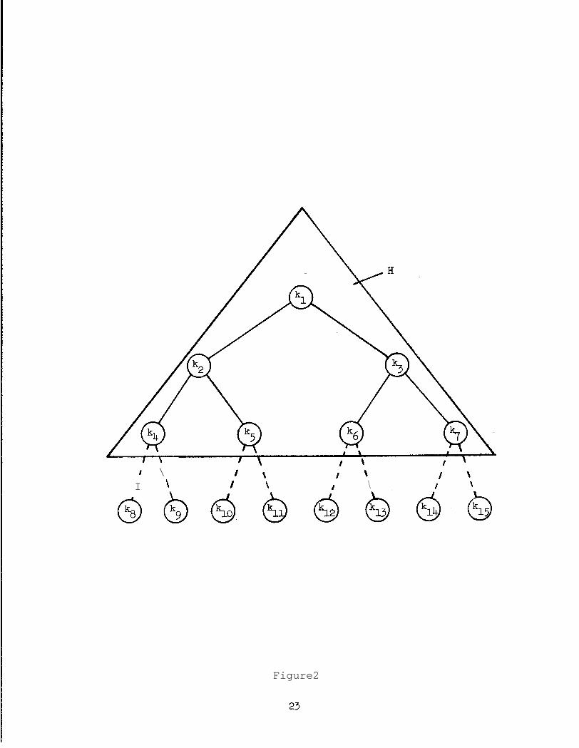
Let us first assume that heap H is random. (See Figure 2.)
When ks is inserted it can exchange with k4 , k2 , and kl . These
are the same nodes that k9
will encounter, hencekY
will be competing
with numbers greater than or equal to k8 % competition. Consequently
the average at node 9 will be smaller than that at node 8 . Let us
now look at the leftmost node of the right subtree, k12 l
When it is
inserted it will be compared with k6 , k3and k1.
The only one of
these nodes that could possibly have been affected by previous insertions
at this level is kl l
But k12 is campared tokl
only when it is
greater than k3 ; therefore we might expect that the average at 12
is only slightly smaller than the average at 8 . By this same kind
of reasoning the average at 15 should be the smallest at this level.
The above discussion shows that the average will have an undulatory
behavior at each level.
22
Page 25
/ \I \ / \ I \ / \
Figure2
23
Page 26
Actually the heap H , as we know, will not be random, but this
will only accentuate such behavior. The heap H is not random because
large keys tend to drift to the right, thus further lessening the
averages of the elements in the right subtree. To see this, consider
the input as a random permutation of [1,2,...,15] . We know that after
all nodes have been inserted, 15 will be at the root, and we shall
examine the chances ofk2 or
5being 14 . We have several cases
to consider. The number 14 will settle as the left son if
(1) 15 and 14 both enter the tree on the left;
(2) one of them enters at the root and the other on the left;
(3) 14 enters on the left and 15 enters previously on the right;
(4) 14 enters on the right and 15 enters later on the left.
Similarly there are four corresponding cases where 14 settles as
the right sonk3 l
Comparing these cases we find that the difference
between the probabilities that 14 settles atk3
rather than k2 is
the probability that 14 enters on the same level as 15 but on the
opposite side.
In order to dampen the latter effect we suggest a "zig-zag" method,
alternating the direction of insertion at each level. Table 1 also
shows the averages found by this "zig-zag" method, when even levels are
inserted from right to left. The effect is to balance the tree more by
1E upsetting the ordinary drift of large elements to the right.
70 Aclmowledgments
The authors wish to thank Prof. Knuth for his guidance and
suggestions throughout the developer& of this research.
Page 27
References
[Knuth - 19681: D. E. Knuth, The Art of Computer programming, Vol. 1
Addison-Wesley, 1968.
[Knuth - 19731: D. E. Knuth, The Art of Computer programmin@;, Vol. 3
Addison-Wesley, 1973.
[WiUA.ams - 19641: Jo W. Jo Wil1ia-m Algorithm 232: HEAPSORT, CACM 7
(@+), 347-348.
25