45
Reachability, Schedulability and Optimality Ansgar Fehnker June 3
| Date post: | 18-Dec-2015 |
| Category: |
Documents |
| View: | 217 times |
| Download: | 3 times |
Reachability, Schedulability and
Optimality
Ansgar Fehnker
June 3
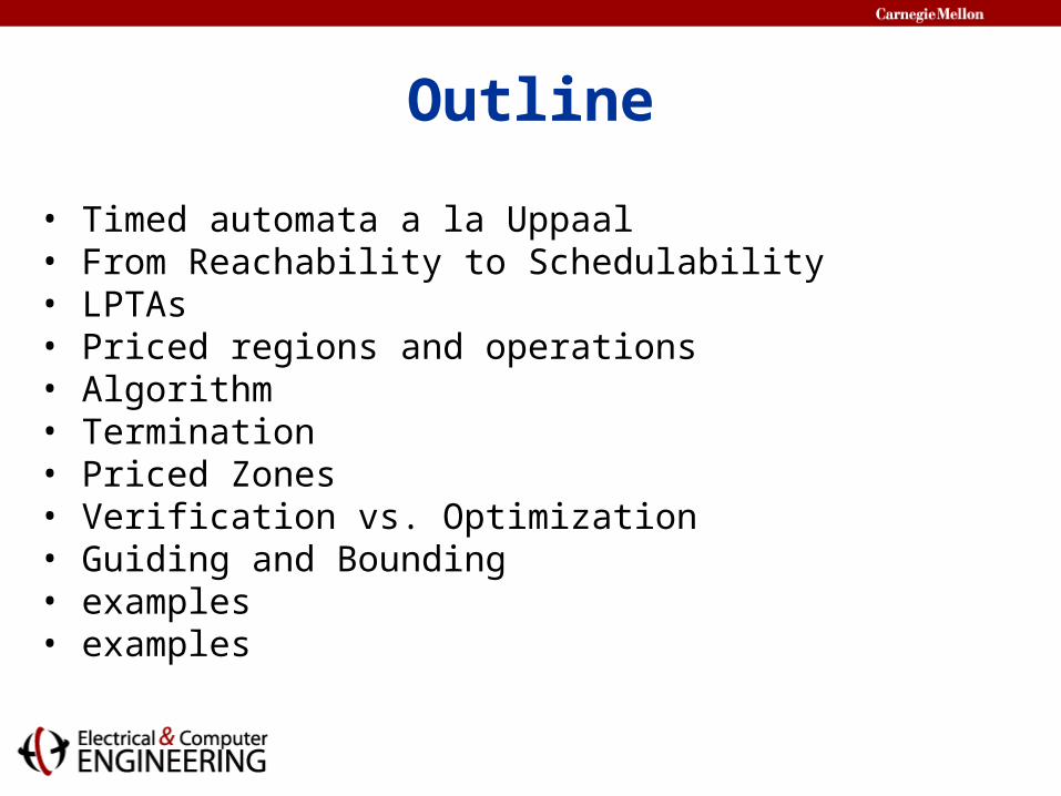
Outline
• Timed automata a la Uppaal• From Reachability to Schedulability• LPTAs• Priced regions and operations• Algorithm• Termination• Priced Zones• Verification vs. Optimization• Guiding and Bounding• examples• examples
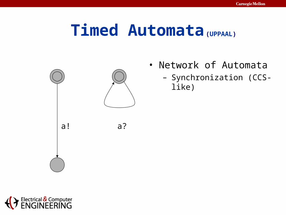
• Network of Automata– Synchronization (CCS-
like)
a! a?
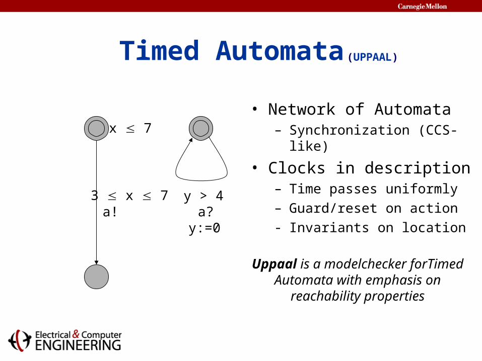
Timed Automata(UPPAAL)
a?y > 4
y:=0a!
3 x 7
x 7
Timed Automata(UPPAAL)
• Network of Automata– Synchronization (CCS-like)
• Clocks in description– Time passes uniformly– Guard/reset on action- Invariants on location
Uppaal is a modelchecker forTimed Automata with emphasis on reachability
properties
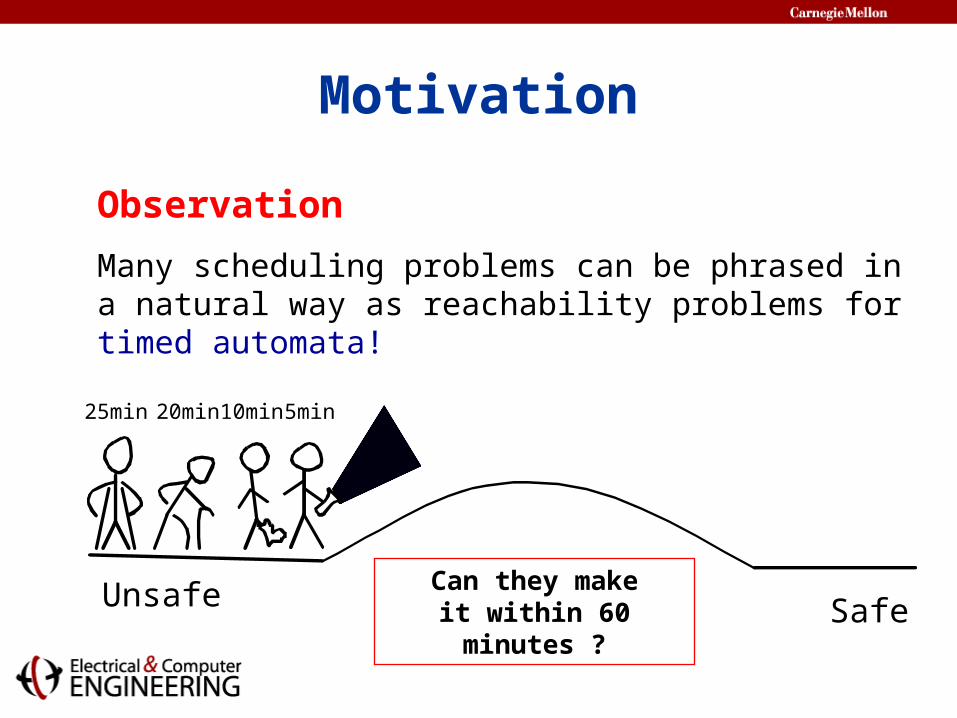
Observation
Many scheduling problems can be phrased in a natural way as reachability problems for timed automata!
Unsafe Safe
25min 20min10min5min
Can they makeit within 60 minutes ?
Motivation
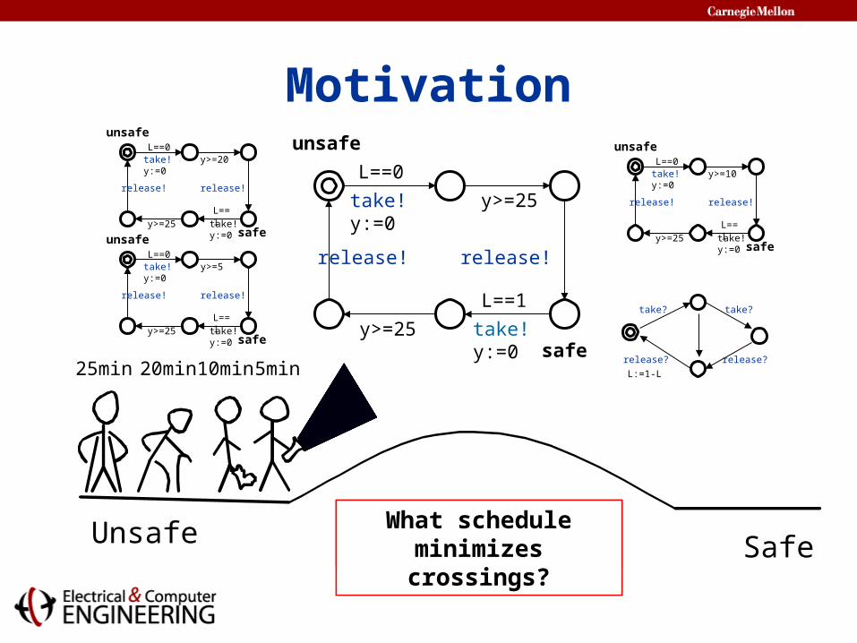
unsafe
L==0
take!y:=0
y>=25
release!
L==1
take!y:=0
y>=25
release!
safe
Unsafe Safe
25min 20min10min5min
Can they makeit within 60 minutes ?
What is the fastest schedule?
Motivation
What schedule mini-mizes unsafe
time?
What schedule minimizes crossings?
unsafeL==0take!y:=0
y>=20
release!
L==1take!y:=0
y>=25
release!
safeunsafe
L==0take!y:=0
y>=5
release!
L==1take!y:=0
y>=25
release!
safe
unsafeL==0take!y:=0
y>=10
release!
L==1take!y:=0
y>=25
release!
safe
take?
release?
take?
release?
L:=1-L

Linearly Priced Timed Automata
• Timed Automata + Costs on transitions and locations.– Cost of performing transition: Transition cost.– Cost of performing delay d: ( d x location cost ).
(a,x=y=0) (b,x=y=0) (b,x=y=2)(2.5)
(a,x=0,y=2)
• Cost of Execution Trace: Sum of costs: 4 + 5 + 0 = 9
b
x<5
y>2
x<3
y:=0a c
4 2.5 x 2 0
cost’=1
cost+=4cost’=0
cost’=2
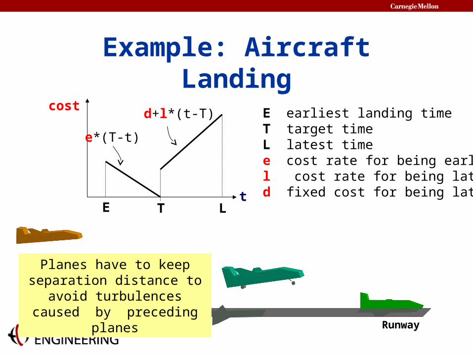
Example: Aircraft Landing
cost
tE LT
E earliest landing timeT target timeL latest timee cost rate for being earlyl cost rate for being lated fixed cost for being late
e*(T-t)
d+l*(t-T)
Planes have to keep separation distance to
avoid turbulences caused by preceding planes
Runway
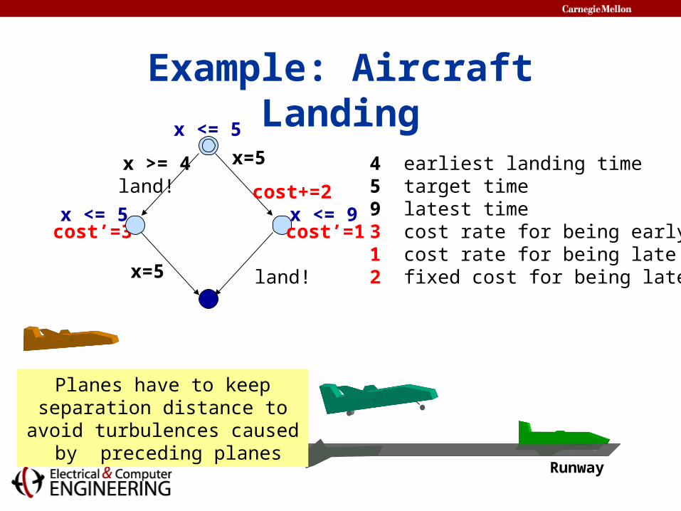
Example: Aircraft Landing
land!x >= 4
x=5
x <= 5
x=5
x <= 5
land!
x <= 9cost+=2
cost’=3 cost’=1
4 earliest landing time5 target time9 latest time3 cost rate for being early1 cost rate for being late2 fixed cost for being late
Planes have to keep separation distance to avoid
turbulences caused by preceding planes
Runway

Symbolic semantics of Linearly Priced Timed Automata
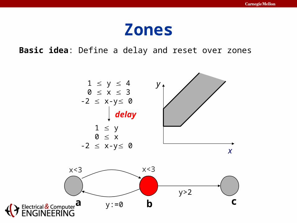
ZonesBasic idea: Define a delay and reset over zones
x<3
y>2
x<3
y:=0a cb
x
y1 y 40 x 3
-2 x-y 0
1 y 0 x
-2 x-y 0
delay
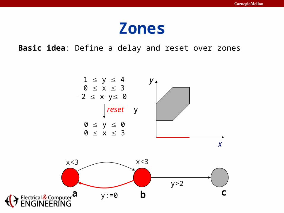
ZonesBasic idea: Define a delay and reset over zones
x<3
y>2
x<3
y:=0a cb
x
y1 y 40 x 3
-2 x-y 0
0 y 00 x 3
reset y
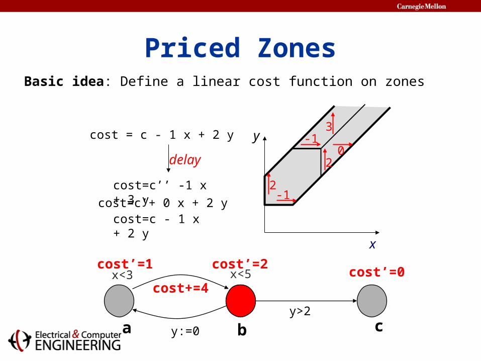
Priced ZonesBasic idea: Define a linear cost function on zones
x<5
y>2
x<3
y:=0a cb
x
ycost = c - 1 x + 2 y
cost’=1
cost+=4cost’=0
cost’=2
cost=c - 1 x + 2 y
cost=c’’ -1 x + 3 ycost=c’+ 0 x + 2 y
delay
2-1
-13
20
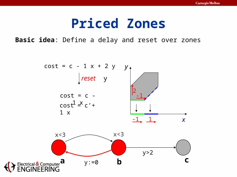
Priced ZonesBasic idea: Define a delay and reset over zones
x<3
y>2
x<3
y:=0a cb
x
ycost = c - 1 x + 2 y
2-1
reset y
-1 1
cost = c’+ 1 x
cost = c - 1 x
State-Space Exploration Algorithm
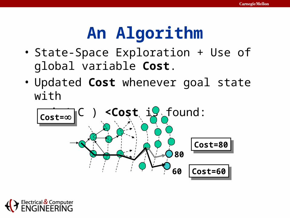
An Algorithm• State-Space Exploration + Use of global
variable Cost.• Updated Cost whenever goal state with min( C ) <Cost is found:
80Cost=80Cost=80
60 Cost=60Cost=60
Cost=Cost=
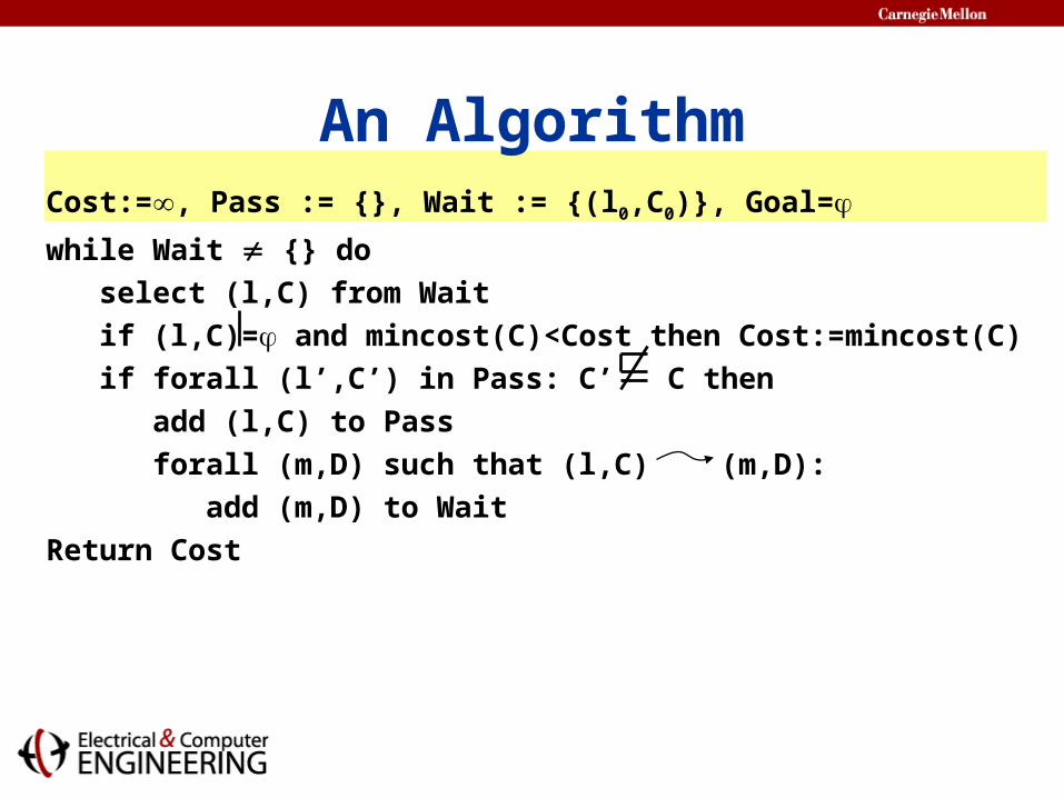
An AlgorithmCost:=, Pass := {}, Wait := {(l0,C0)}, Goal=
while Wait {} do select (l,C) from Wait
if (l,C)= and mincost(C)<Cost then Cost:=mincost(C) if forall (l’,C’) in Pass: C’ C then
add (l,C) to Pass
forall (m,D) such that (l,C) (m,D):
add (m,D) to Wait
Return Cost
Cost:=, Pass := {}, Wait := {(l0,C0)}, Goal=
while Wait {} do select (l,C) from Wait
if (l,C)= and mincost(C)<Cost then Cost:=mincost(C) if forall (l’,C’) in Pass: C’ C then
add (l,C) to Pass
forall (m,D) such that (l,C) (m,D):
add (m,D) to Wait
Return Cost
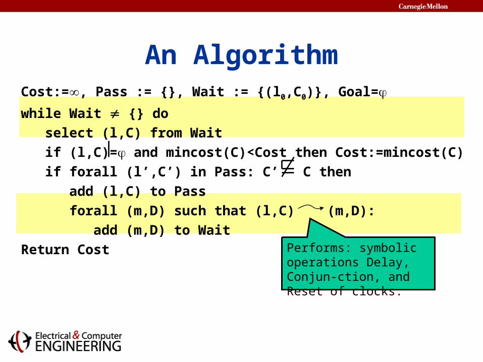
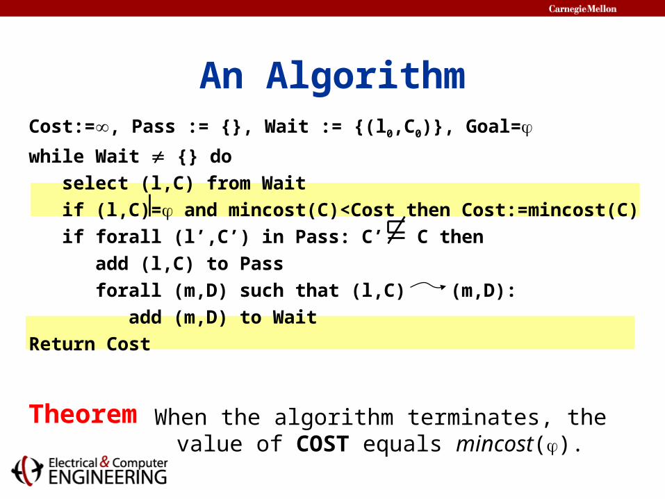
An Algorithm
Performs: symbolic operations Delay, Conjun-ction, and Reset of clocks.
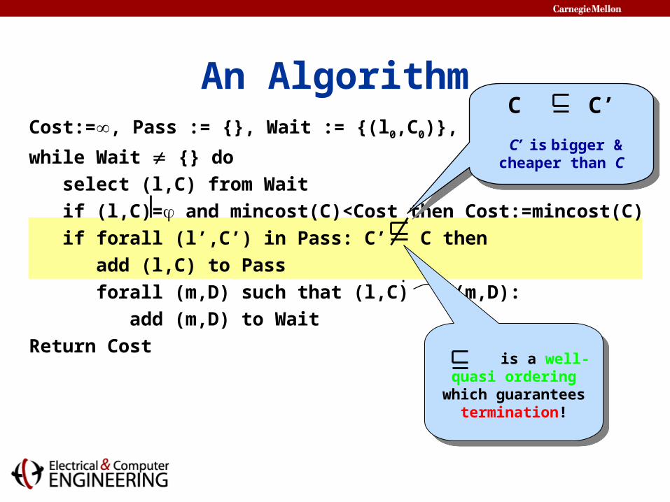
Cost:=, Pass := {}, Wait := {(l0,C0)}, Goal=
while Wait {} do select (l,C) from Wait
if (l,C)= and mincost(C)<Cost then Cost:=mincost(C) if forall (l’,C’) in Pass: C’ C then
add (l,C) to Pass
forall (m,D) such that (l,C) (m,D):
add (m,D) to Wait
Return Cost
.
An AlgorithmC C’
C’ is bigger & cheaper than C
C C’
C’ is bigger & cheaper than C
is a well-quasi ordering
which guarantees termination!
is a well-quasi ordering
which guarantees termination!
An AlgorithmCost:=, Pass := {}, Wait := {(l0,C0)}, Goal=
while Wait {} do select (l,C) from Wait
if (l,C)= and mincost(C)<Cost then Cost:=mincost(C) if forall (l’,C’) in Pass: C’ C then
add (l,C) to Pass
forall (m,D) such that (l,C) (m,D):
add (m,D) to Wait
Return Cost
TheoremWhen the algorithm terminates, the value of COST equals mincost().
Efficient Reachability of LPTAs
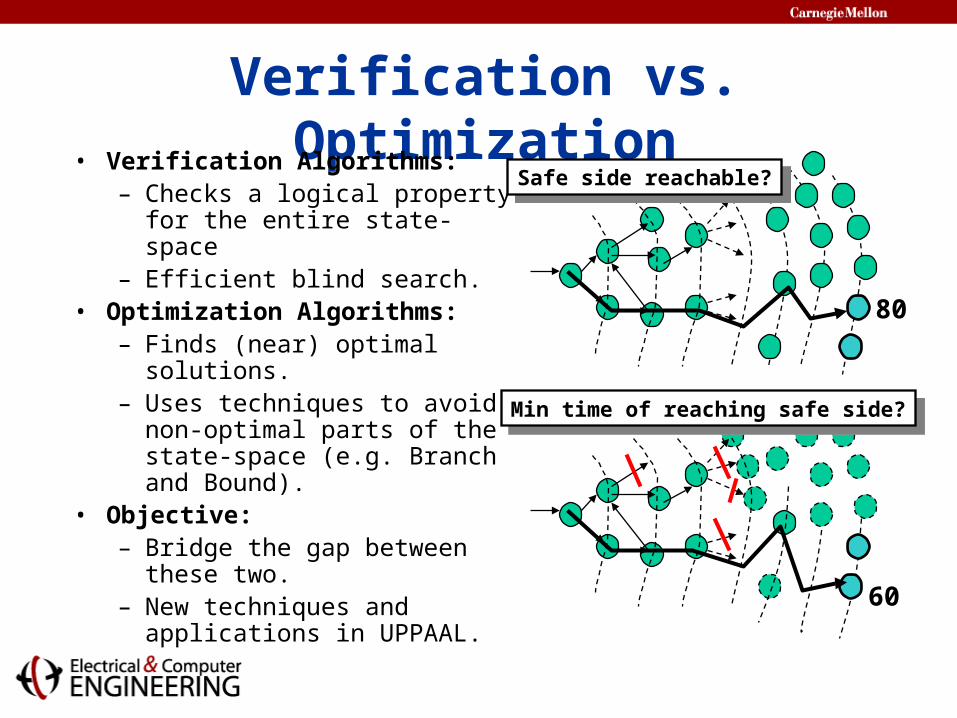
Verification vs. Optimization• Verification Algorithms:
– Checks a logical property for the entire state-space
– Efficient blind search.• Optimization Algorithms:
– Finds (near) optimal solutions.
– Uses techniques to avoid non-optimal parts of the state-space (e.g. Branch and Bound).
• Objective: – Bridge the gap between
these two.– New techniques and
applications in UPPAAL.
80
60
Safe side reachable?Safe side reachable?
Min time of reaching safe side?Min time of reaching safe side?
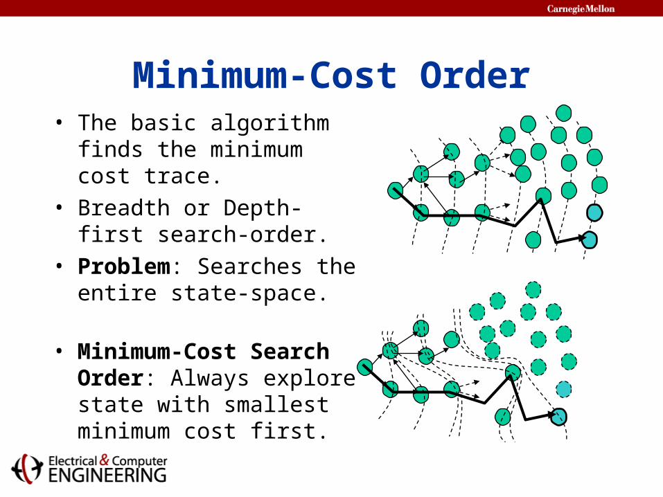
Minimum-Cost Order• The basic algorithm finds
the minimum cost trace.• Breadth or Depth-first
search-order.• Problem: Searches the
entire state-space.
• Minimum-Cost Search Order: Always explore state with smallest minimum cost first.
Fact: First found goal state is optimal.
• Cost grows along all paths.• The search can terminate when first goal state
found.• Like Dijkstra’s shortest path algorithm.
• Simpler algorithm: variable Cost no longer needed.
Minimum-Cost Order
Estimates of Remaining Cost
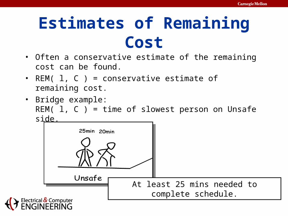
• Often a conservative estimate of the remaining cost can be found.
• REM( l, C ) = conservative estimate of remaining cost.• Bridge example:
REM( l, C ) = time of slowest person on Unsafe side.
At least 25 mins needed to complete schedule.
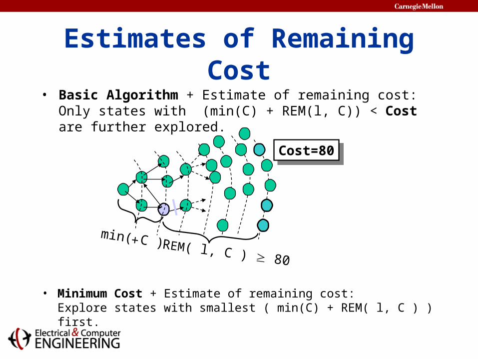
Estimates of Remaining Cost
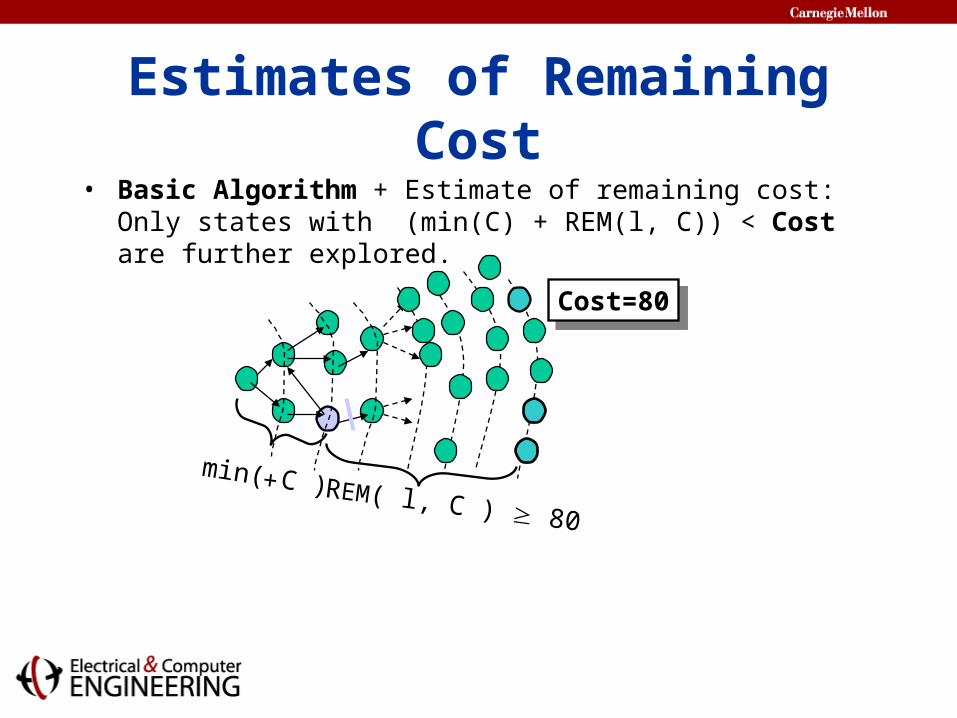
• Basic Algorithm + Estimate of remaining cost:Only states with (min(C) + REM(l, C)) < Cost are further explored.
Cost=80Cost=80
+ REM( l, C ) 80
min( C )
Estimates of Remaining Cost
• Minimum Cost + Estimate of remaining cost:Explore states with smallest ( min(C) + REM( l, C ) ) first.
Cost=80Cost=80
+ REM( l, C ) 80
min( C )
• Basic Algorithm + Estimate of remaining cost:Only states with (min(C) + REM(l, C)) < Cost are further explored.
Using Heuristics• Allows the users to control the search order
according to heuristics. • Symbolic states extended to (l, C, h), where
h is the priority of a state.• Transitions are annotated with assignments to
h.• Flexible!
Basic Algorithm + Heuristics: State with highest h is explored first.
Examples
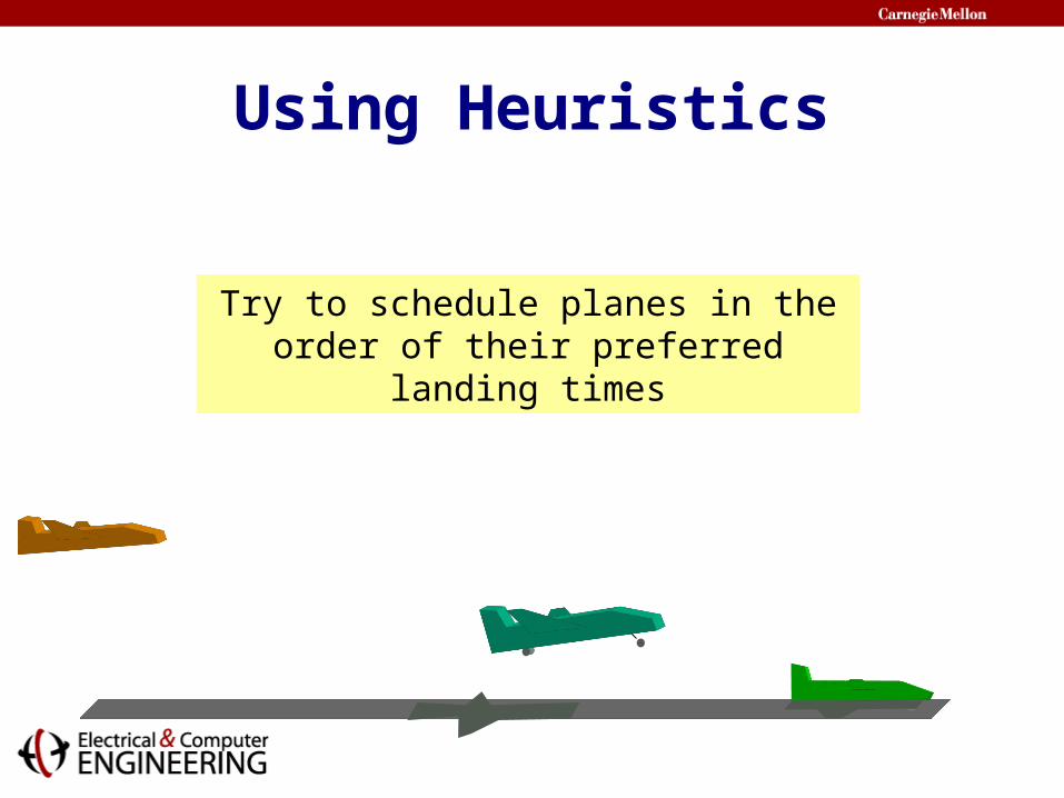
Using Heuristics
Try to schedule planes in the order of their preferred landing times
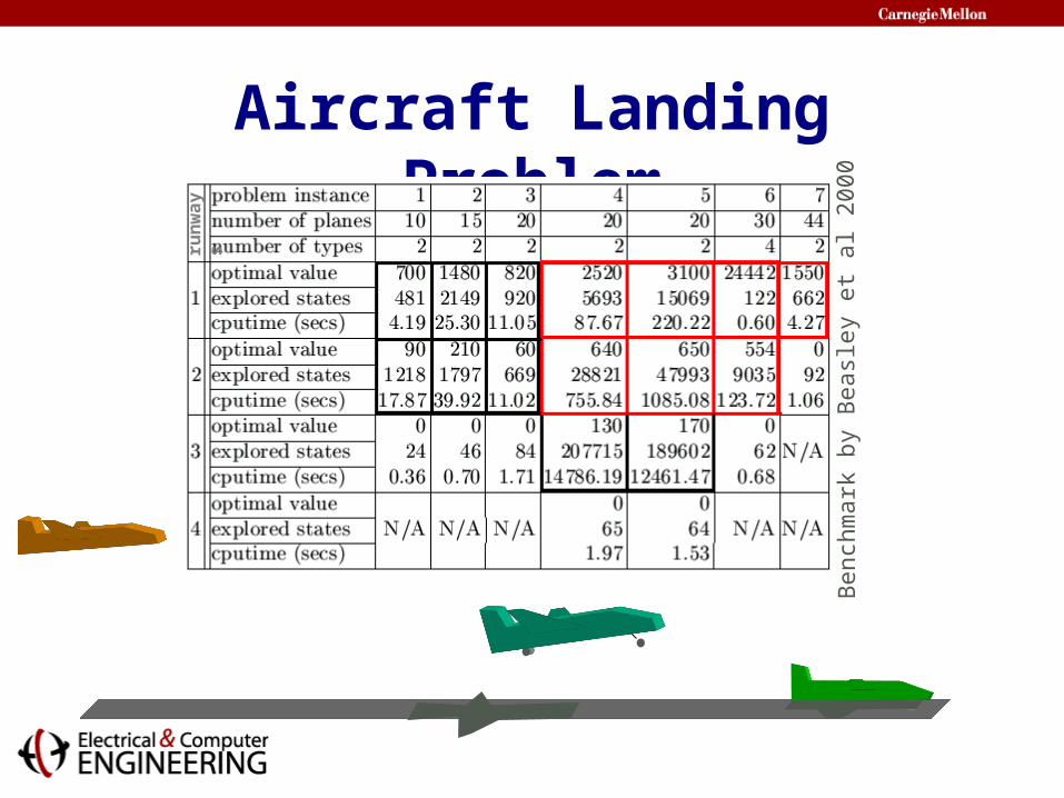
Aircraft Landing Problemrunways
Bench
mark
by B
easl
ey e
t al 2
00
0
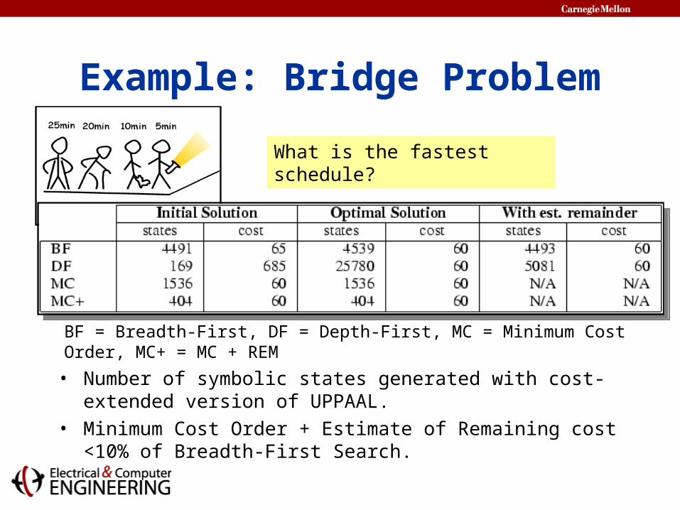
Example: Bridge Problem
• Number of symbolic states generated with cost-extended version of UPPAAL.
• Minimum Cost Order + Estimate of Remaining cost<10% of Breadth-First Search.
BF = Breadth-First, DF = Depth-First, MC = Minimum Cost Order, MC+ = MC + REM
What is the fastest schedule?
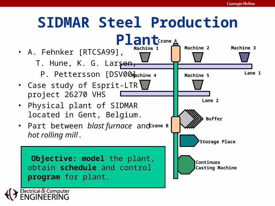
Machine 1 Machine 2 Machine 3
Machine 4 Machine 5
Buffer
Continuos Casting Machine
Storage Place
Crane B
Crane A
• A. Fehnker [RTCSA99], T. Hune, K. G. Larsen, P. Pettersson [DSV00]• Case study of Esprit-LTR
project 26270 VHS• Physical plant of SIDMAR
located in Gent, Belgium.• Part between blast furnace and
hot rolling mill.
Objective: model the plant, obtain schedule and control program for plant.
Lane 1
Lane 2
SIDMAR Steel Production Plant
Machine 1 Machine 2 Machine 3
Machine 4 Machine 5
Buffer
Continuos Casting Machine
Storage Place
Crane B
Crane A
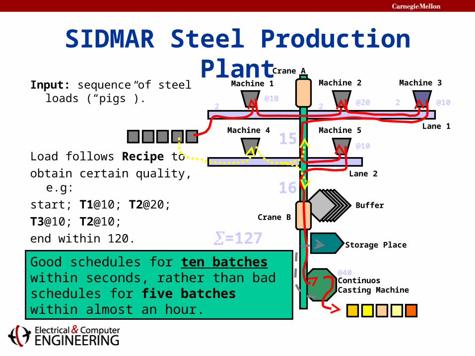
Input: sequence of steel loads (“pigs”). @10 @20 @10
@10
@40
Load follows Recipe to obtain certain quality, e.g:start; T1@10; T2@20; T3@10; T2@10; end within 120.
Output: sequence of higher quality steel.
Lane 1
Lane 2
2 2 2
15
16
=127
SIDMAR Steel Production Plant
Good schedules for ten batches within seconds, rather than bad schedules for five batches within almost an hour.
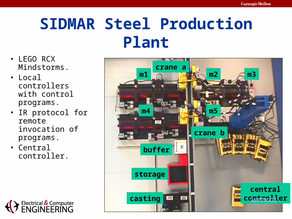
• LEGO RCX Mindstorms.
• Local controllers with control programs.
• IR protocol for remote invocation of programs.
• Central controller.
m1 m2 m3
m4 m5
crane a
crane b
casting
storage
buffer
centralcontrollerSynthesis
SIDMAR Steel Production Plant
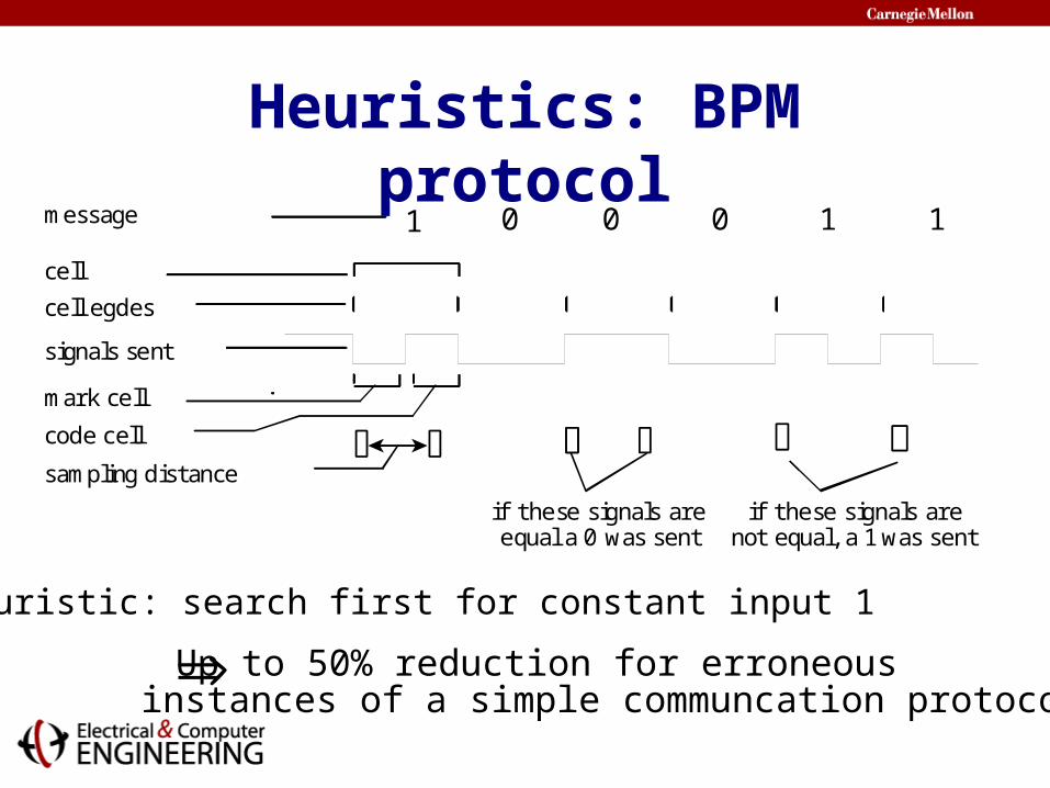
Heuristic: search first for constant input 1
Up to 50% reduction for erroneousinstances of a simple communcation protocol.
0 001 11message
cell
cell egdes
signals sent
mark cell
code cell
sampling distance
if these signals are equal a 0 was sent
if these signals arenot equal, a 1 was sent
Heuristics: BPM protocol
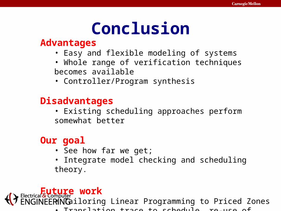
Advantages• Easy and flexible modeling of systems• Whole range of verification techniques becomes available• Controller/Program synthesis
Disadvantages• Existing scheduling approaches perform somewhat better
Our goal• See how far we get;• Integrate model checking and scheduling theory.
Future work• Tailoring Linear Programming to Priced Zones• Translation trace to schedule, re-use of schedules, ...
Conclusion
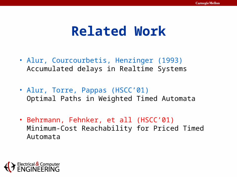
Related Work
• Alur, Courcourbetis, Henzinger (1993)Accumulated delays in Realtime Systems
• Alur, Torre, Pappas (HSCC’01)Optimal Paths in Weighted Timed Automata
• Behrmann, Fehnker, et all (HSCC’01)Minimum-Cost Reachability for Priced Timed Automata
Related Work (cont)
• Asarin & Maler (1999)Time optimal control using backwards fixed point computation
• Niebert, Tripakis & Yovine (2000)Minimum-time reachability using forward reachability
• Behrmann, Fehnker et all (TACAS’2001, CAV’01)Minimum-time reachability using Branch-and-Bound
• Brinksma, Maler, Fehnker(STTT02)Using UPPAAL en SPIN to compute optimal schedules.
• Abdeddaim, Maler (CAV’01)Job-Shop Scheduling using Timed Automata
• General Trend (AAAI’01): Integrating Scheduling/Planning and Model Checking
End of slide show
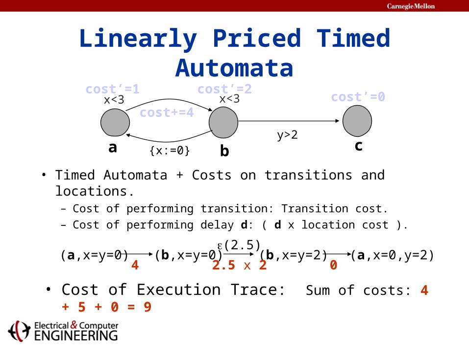
Linearly Priced Timed Automata
• Timed Automata + Costs on transitions and locations.– Cost of performing transition: Transition cost.– Cost of performing delay d: ( d x location cost ).
(a,x=y=0) (b,x=y=0) (b,x=y=2)(2.5)
(a,x=0,y=2)4 2.5 x 2 0
• Cost of Execution Trace: Sum of costs: 4 + 5 + 0 = 9
b
x<3
y>2
x<3
{x:=0}a c
cost’=1
cost+=4cost’=0
cost’=2

Regions
x<3
y>2a b c{x:=0}
x<3
x
y
1 2
3
1
2
3
4
5
4 50
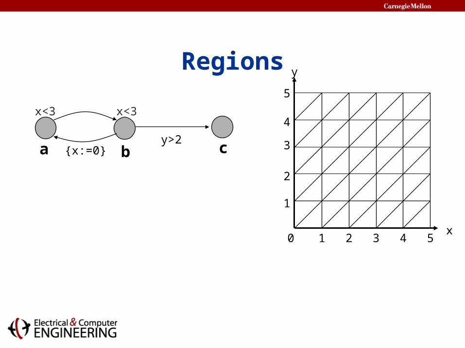
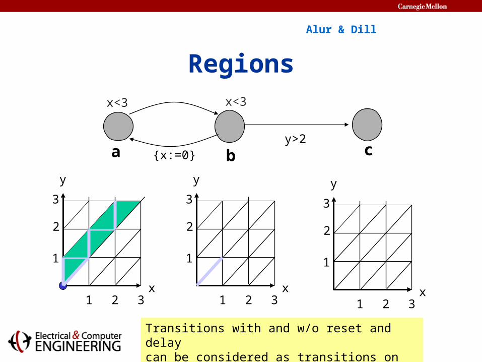
Regions
x<3
y>2a b c{x:=0}
x<3
x
y
1 2
3
1
2
3
4
5
4 50
x
3
1
2
Transitions with and w/o reset and delay can be considered as transitions on regions!
y
1 2
Alur & Dill
x<3
y>2a b c
3x
3
1
2
y
x
3
1
2
y
1 2 3 1 2 3
x<3
{x:=0}
Regions


