Louisiana State UniversityLSU Digital Commons

LSU Historical Dissertations and Theses Graduate School

1989

Real-Time Effective Stress Evaluation in Shales:Pore Pressure and Permeability Estimation.Jean-louis Jerome AlixantLouisiana State University and Agricultural & Mechanical College

Follow this and additional works at: https://digitalcommons.lsu.edu/gradschool_disstheses

This Dissertation is brought to you for free and open access by the Graduate School at LSU Digital Commons. It has been accepted for inclusion inLSU Historical Dissertations and Theses by an authorized administrator of LSU Digital Commons. For more information, please contactgradetd@lsu.edu.

Recommended CitationAlixant, Jean-louis Jerome, "Real-Time Effective Stress Evaluation in Shales: Pore Pressure and Permeability Estimation." (1989). LSUHistorical Dissertations and Theses. 4828.https://digitalcommons.lsu.edu/gradschool_disstheses/4828

INFORMATION TO USERS

The most advanced technology has been used to photograph and reproduce this manuscript from the microfilm master. UM1 films the text directly from the original or copy submitted. Thus, some thesis and dissertation copies are in typewriter face, while others may be from any type of computer printer.

The quality of this reproduction is dependent upon the quality of the copy submitted. Broken or indistinct print, colored or poor quality illustrations and photographs, print bleedthrough, substandard margins, and improper alignment can adversely affect reproductioa

In the unlikely event that the author did hot send UMI a complete manuscript and there are missing pages, these will be noted. Also, if unauthorized copyright material had to be removed, a note will indicate the deletion.

Oversize materials (e.g., maps, drawings, charts) are reproduced by sectioning the original, beginning at the upper left-hand corner and continuing from left to right in equal sections with small overlaps. Each original is also photographed in one exposure and is included in reduced form at the back of the book.

Photographs included in the original manuscript have been reproduced xerographically in this copy. Higher quality 6" x 9" black and white photographic prints are available for any photographs or illustrations appearing in this copy for an additional charge. Contact UMI directly to order.

University Microfilms Inlernationa!A Bell & Howell Information Company

300 North Zeeb Road. Ann Arbor, Ml 48106-1346 USA 313/761-4700 800/521-0600

O rder N um ber 9025288i .

Real-tim e effective stress evaluation in shales: Pore pressure and perm eability estim ation

Alixant, Jean-Louis Jerome, Ph.D.

The Louisiana State University and Agricultural and Mechanical Col., 1989

Copyright © 1989 by A lix a n t, Jean-Louis Jerome. A ll rights reserved.

U MI300 N. ZeebRd.Ann Arbor, MI 48106

REAL-TIME EFFECTIVE STRESS EVALUATION IN SHALES:

PORE PRESSURE AND PERMEABILITY ESTIMATION

A Dissertation

Submitted to the Graduate Faculty of the Louisiana State University and

Agricultural and Mechanical College in partial fulfillment of the

requirements for the degree of Doctor of Philosophy

in

The Department! of Petroleum Engineering

by

Jean-Louis Alixant IngSnieur Institut Industriel du Nord, 1986

Ing6nieur Ecole Nationale Supgrieure du P6trole et des Moteurs, 1987December 1989

ACKNOWLEDGMENTS

The author wishes to express his deepest gratitude to Dr. Robert

Desbrandes, who supervised this research. Dr. Desbrandes provided fine

advice and timely suggestions rather than a rigid guidance, thus allowing the

author to develop his own research skills. Sincere appreciation is extended to

Dr. Adam T. Bourgoyne, Jr., Dr. Julius Langlinais, and Dr. Andrew K.

Wojtanowicz for pertinent and appropriate suggestions throughout the duration

of this project. The author also thanks his minor Professor, Dr. G. Hart, for help

and guidance in Geology. As the outside committee member, Dr. A. Lewis is

acknowledged for his efforts and thorough review of the manuscript.

The author is gratefully indebted to Total Compagnie Frangaise des

P6troles for financial support. In particular, the author wishes to recognize the

help of Patrick Toutain, who obtained the necessary funds for financial support,

and Thierry Delahaye, who provided technical support and advice. The author

also acknowledges the Louisiana State University Mineral Research Institute for

providing an assistanship.

Many individuals have participated in this research since it started in

January 1988. Whether at LSU or in the industry, these individuals are also

acknowledged here. Among them, Dr. Jesse Jaynes has provided decisive

help by lending his invaluable film printer on many occasions. Miss Dayna

Darby is thanked for patiently editing the original manuscript.

Finally, the author wishes to express his deepest appreciation and love

to his parents whose endless support and encouragement helped complete this

work. To them and to Nicole, the author dedicates this research.

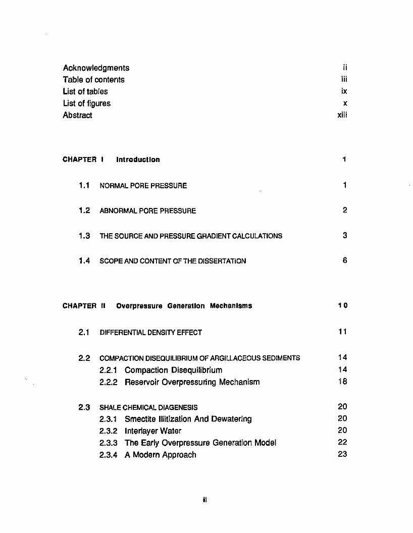
Acknowledgments iiTable of contents iiiList of tables ixList of figures xAbstract xiii

CHAPTER I Introduction 1

1.1 NORMAL PORE PRESSURE 1

1.2 ABNORMAL PORE PRESSURE 2

1.3 THE SOURCE AND PRESSURE GRADIENT CALCULATIONS 3

1.4 SCOPE AND CONTENT OF THE DISSERTATION 6

CHAPTER ll Overpressure Generation Mechanisms 10

2.1 DIFFERENTIAL DENSITY EFFECT 11

2.2 COMPACTION DISEQUILIBRIUM OF ARGILLACEOUS SEDIMENTS 14

2.2.1 Compaction Disequilibrium 142.2.2 Reservoir Overpressuring Mechanism 18

2.3 SHALE CHEMICAL DIAGENESIS 20

2.3.1 Smectite lliitization And Dewatering 202.3.2 Interlayer Water 202.3.3 The Early Overpressure Generation Model 222.3.4 A Modern Approach 23

ii

2.4 AQUATHERMAL PRESSURING 24

2.4.1 The Model 242.4.2 Limitations 29

2.5 TECTONIC ACTIVITY 30

2.6 OTHER POSSIBLE CAUSES OF OVERPRESSURES 30

2.7 A NUMERICAL MODEL OF OVERPRESSURING IN SHALES 31

2.8 CONCLUSION: CHARACTERISTICS OF OVERPRESSURED SHALES 32

2.8.1 Effective Overpressure Mechanisms 322.8.2 Selection Of A Pore Pressure Indicator 34

CHAPTER III Pore Pressure Evaluation Options 3 6

3.1 PORE PRESSURE EVALUATION USING RESISTIVITY LOGS 36

3.1.1 Overpressure Detection 363.1.2 Empirical Evaluation Of Pore Pressure Magnitude 393.1.3 Theoretical Interpretation 433.1.4 The Variable Overburden Gradient 463.1.5 Conclusion 49

3.2 PORE PRESSURE EVALUATION USING DRILLING DATA 50

3.2.1 Rate Of Penetration And Pore Pressure 513.2.2 The d-exponent 523.2.3 Mud Weight Correction 563.2.4 Bit Wear Correction 583.2.5 Other Attempts 593.2.6 Conclusion 59

iv

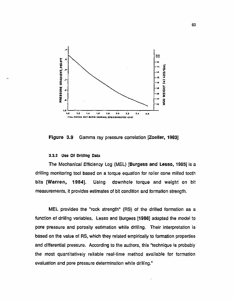
3.3 REAL-TIME PORE PRESSURE EVALUATION3.3.1 Pore Pressure From Gamma Ray Measurements3.3.2 Use Of Drilling Data3.3.3 Use Of Resistivity Measurements

3.4 CONCLUSION

CHAPTER IV Real-Time Effective Vertical Stress Evaluation In Shales

4.1 REAL-TIME REQUIREMENTS

4.1.1 Use Of Normal Trend Lines4.1.2 Selection Of A Real-Time Measurement4.1.3 General Strategy

4.2 THE ELECTRICAL MODULE

4.2.1 The Diffuse Double Layer Theory4.2.2 Compacting Clay Minerals4.2.3 Expected Shale Porosity4.2.4 Formation Factor Relationship For Shales4.2.5 Bound Water Resistivity4.2.6 Determination Of Shale Porosity

4.3 THE MECHANICAL MODULE

4.3.1 The Effective Stress Concept4.3.2 Derivation Of Terzaghi's Relationship4.3.3 One-Dimensional Compaction4.3.4 Shale Compression Law

4.4 SUMMARY AND EXAMPLE

4.4.1 Assumptions4.4.2 Procedure4.4.3 Example

60616364

66

67

67677072

757578818793

95

979899

106 112

113113114115

v

CHAPTER V Real-Time Pore Pressure Evaluation: Field Cases 119

5.1 DATA ACQUISITION AND PROCESSING 119

5.1.1 Calibration Coefficients 1205.1.2 Shale Discrimination 1215.1.3 Resistivity 1225.1.4 Temperature Gradients 1235.1.5 Overburden 1235.1.6 Depth Data 1235.1.7 Pressure Measurements 1245.1.8 Data Processing 124

5.2 FIELD EXAMPLES 124

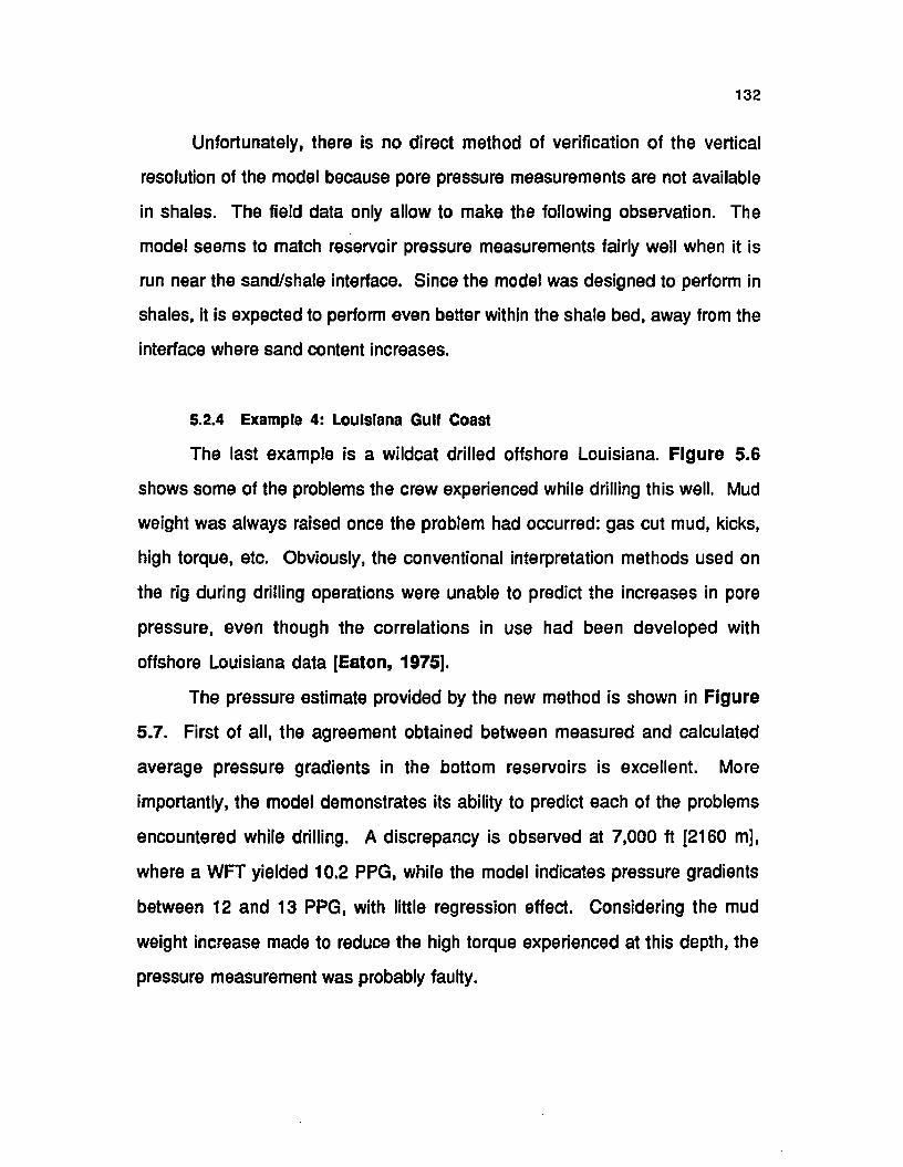
5.2.1 Example 1: North Sea 1255.2.2 Example 2: Texas Gulf Coast 1285.2.3 Example 3: Offshore Egypt 1305.2.4 Example 4: Louisiana Gulf Coast 132

5.3 CONCLUSION 134

CHAPTER VI Shale Permeability Estimation 136

6.1 DEEP-WELL INJECTION 1376.1.1 Definition 1376.1.2 Regulations 138

6.2 PERMEABILITY AND EFFECTIVE STRESS CORRELATION 141

6.2.1 Shale Permeability 1416.2.2 Permeability And Effective Stress 141

6.3 ESTIMATING SHALE PERMEABILITY 143

6.3.1 General Approach 143

vi

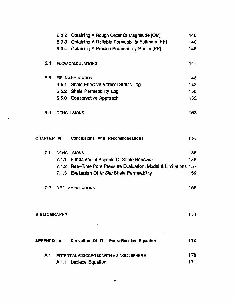
6.3.2 Obtaining A Rough Order Of Magnitude [OM] 1456.3.3 Obtaining A Reliable Permeability Estimate [PE] 1466.3.4 Obtaining A Precise Permeability Profile [PP] 146

6.4 FLOW CALCULATIONS 147

6.5 FIELD APPLICATION 148

6.5.1 Shale Effective Vertical Stress Log 1486.5.2 Shale Permeability Log 1506.5.3 Conservative Approach 152

6.6 CONCLUSIONS 153

CHAPTER VII Conclusions And Recommendations 156

7.1 CONCLUSIONS 156

7.1.1 Fundamental Aspects Of Shale Behavior 1567.1.2 Real-Time Pore Pressure Evaluation: Model & Limitations 1577.1.3 Evaluation Of In Situ Shale Permeability 159

7.2 RECOMMENDATIONS 159

BIBLIOGRAPHY 161

APPENDIX A Derivation Of The Perez-Rosales Equation 170

A. 1 POTENTIAL ASSOCIATED WITH A SINGLE SPHERE 170A.1.1 Laplace Equation 171

vii

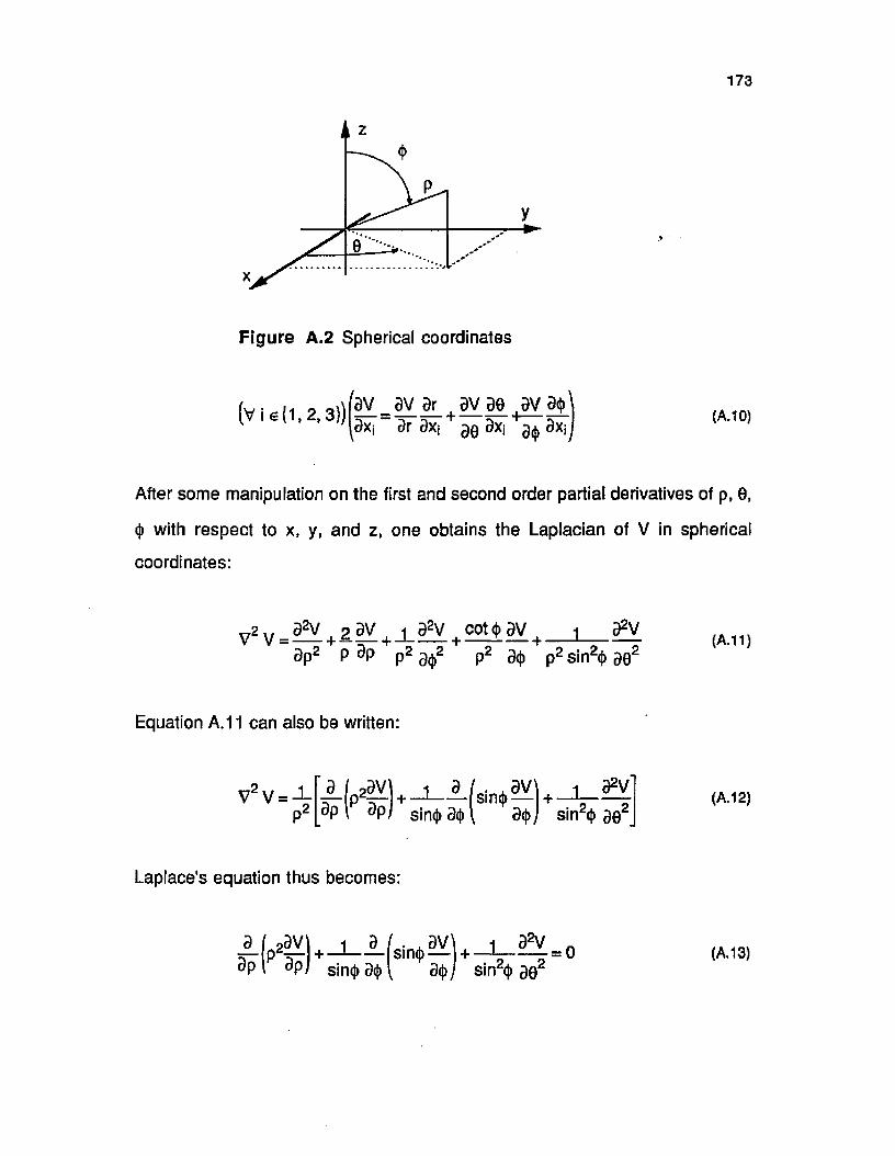
A. 1.2 Laplace Equation In Spherical Coordinates 172A.1.3 Governing Equation 174A. 1.4 Cauchy's Equation 175A. 1.5 Legendre's Equation 176A.1.6 General Solution To Laplace's Equation 183A.1.7 Boundary Conditions And Solution 183

A.2 FORMATION FACTOR RELATIONSHIP 185A.2.1 Potential Associated With A Suspension Of Spheres 185A.2.2 Generalization Of Fricke's Equation 188

APPENDIX B Borehole Mechanical Effects WithinThe Depth Of Investigation Of A 2 MHz Resistivity Tool 190

B. 1 DEPTH OF INVESTIGATION OF 2*MHz TOOLS IN SHALES 191

B.1.1 Simplifying Assumptions 191B.1.2 Electric Propagation In A Conductive Medium 191B.1.3 Skin Effect 193

B.2 STRESSES AROUND A WELLBORE 194B.2.1 Simplifying Assumptions 194

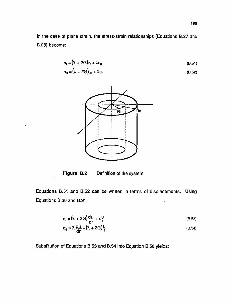
B.2.2 Stress-Strain Relationships in Cylindrical Coordinates 194B.2.3 The Equations Of Equilibrium 195B.2.4 Stresses In The Vicinity Of A Vertical Wellbore 198

B.3 STRESSES WITHIN THE INVESTIGATION RANGE OF THE 2-MHz TOOL 201B.3.1 Numerical Estimate Of Effective Skin Depth 201B.3.2 Numerical Examples Of Stresses Around Boreholes 202B.3.3 Conclusion 208

VITA 210

vlii

LIST OF TABLES

Table

1.1

2.14.1

4.2

4.3e*.

4.4

5.15.2

6.1 B.1

B.2

B.3

B.4

Page

2 Normal formation pressure gradients for several areas of active drilling [Bourgoyne e ta l, 1986].

13 Differential density effect calculation summary.79 Loss of interlayer water layers under subsurface

temperature and pressure conditions.83 Porosity as a function of water layers. Direct calculation

using interlayer and basal spacings.86 Porosity as a function of water layers. Calculation using

specific areas.88 Usual formation factor expressions [Schlumberger,

1988].120 Calibration coefficients used for field tests.128 Pore pressure gradient estimates at 5,000 ft [1524 m].152 Permeability estimation at 5,400 ft [1646 m].207 Example calculations of radial and tangential stresses

around a 8 1/2" wellbore at a distance equal to one third of the approximate effective skin depth.

207 Example calculations of radial and tangential stresses

around a 12 1/4" wellbore at a distance equal to one third of the approximate effective skin depth.

208 Example calculations of radial and tangential stresses

around a 8 1/2" wellbore at a distance equal to the

approximate effective skin depth, 14".208 Example calculations of radial and tangential stresses

around a 12 1/4" wellbore at a distance equal to the

approximate effective skin depth, 14".

ix

I

LIST OF FIGURES

Figure Page

1.1.a 5 The wellsite is higher than the source and the fluid-bearing

formation is hit above the water table.1.1.b 5 The wellsite is higher than the source and the fluid-bearing

formation is hit below the water table.1.1.C 5 The wellsite is lower than the source.2.1 13 Differential density effect.2.2 17 The stages of shale compaction.2.2.a 17 Deposition: clay.2.2.b 17 Increase in overburden weight: claystone.2.2.C 17 Final compaction: shale.2.3 21 2:1 layers and interlayer hydrated cations.2.4 22 Interlayer water ordering [Whittaker, 1985].2.5 26 Pressure and temperature evolution in an open system.2.6 28 Pressure and temperature evolution in a closed system:

PTD diagram [Barker, 1972].3.1 37 Overpressure and resistivity.3.2 38 Overpressures cause shale resistivity to depart from the

normal trend.3.3 39 Normal resistivity.3.4 40 Hottmann and Johnson's [1965] resistivity correlation.3.5 41 Relating shale resistivity data to average reservoir pressure

gradient.3.6 44 The equivalent depth principle.3.7 47 Overburden data for several areas [Bourgoyne et ah

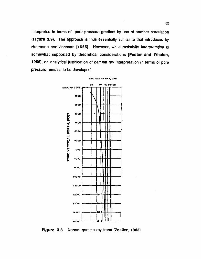
1986].3.8 62 Normal gamma ray trend [Zoeller, 1983].3.9 63 Gamma ray pressure correlation [Zoeller, 1983].4.1 69 Early real-time resistivity interpretation.

x

Figure Page

4.2 69 Real-time resistivity interpretation after drilling into the overpressured zone.

4.3 76 Cation distribution in the vicinity of a clay particle.4.4 78 Interaction between adjacent clay particles.4.5 82 Definition of spacings.4.6 83 Basal spacing as a function of water layers [Sposito and

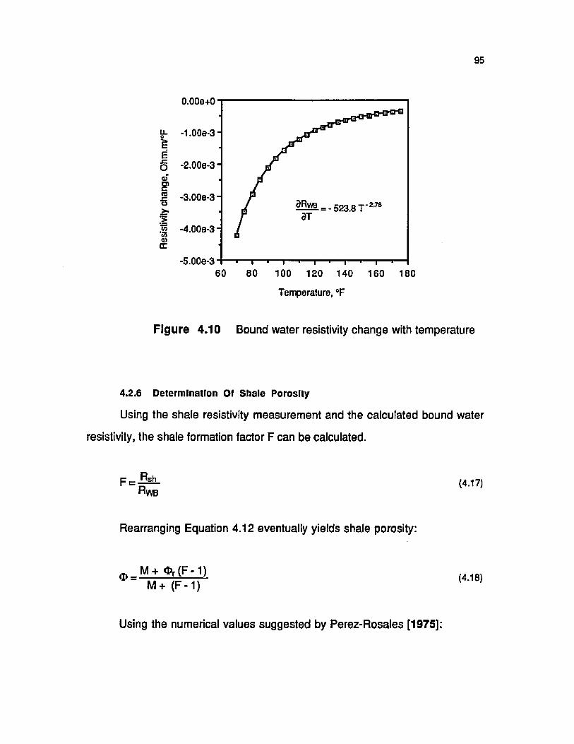
Prost, 1982].4.7 84 Definition of the specific areas of smectite.4.8 92 Comparison of Archie and Perez-Rosales relationships.4.9 94 Bound water resistivity data [Clavier et a!, 1977].4.10 95 Bound water resistivity change with temperature.4.11 100 Force balance in porous media.4.12 101 Cross-section of porous media.4.13 102 Porous media geometry and stress distribution.4.14 103 Pore pressure distribution on solid grain surfaces.4.15 108 Relationship between void ratio and effective stress for one­

dimensional compression of cohesive soils.4.16 109 Relationship between void ratio and effective stress for one­

dimensional compression of cohesive soils.4.17 110 Relationship between void ratio and effective stress for high

stress level one-dimensional compression of shales.4.18 111 The virgin compression curve can be approximated by a

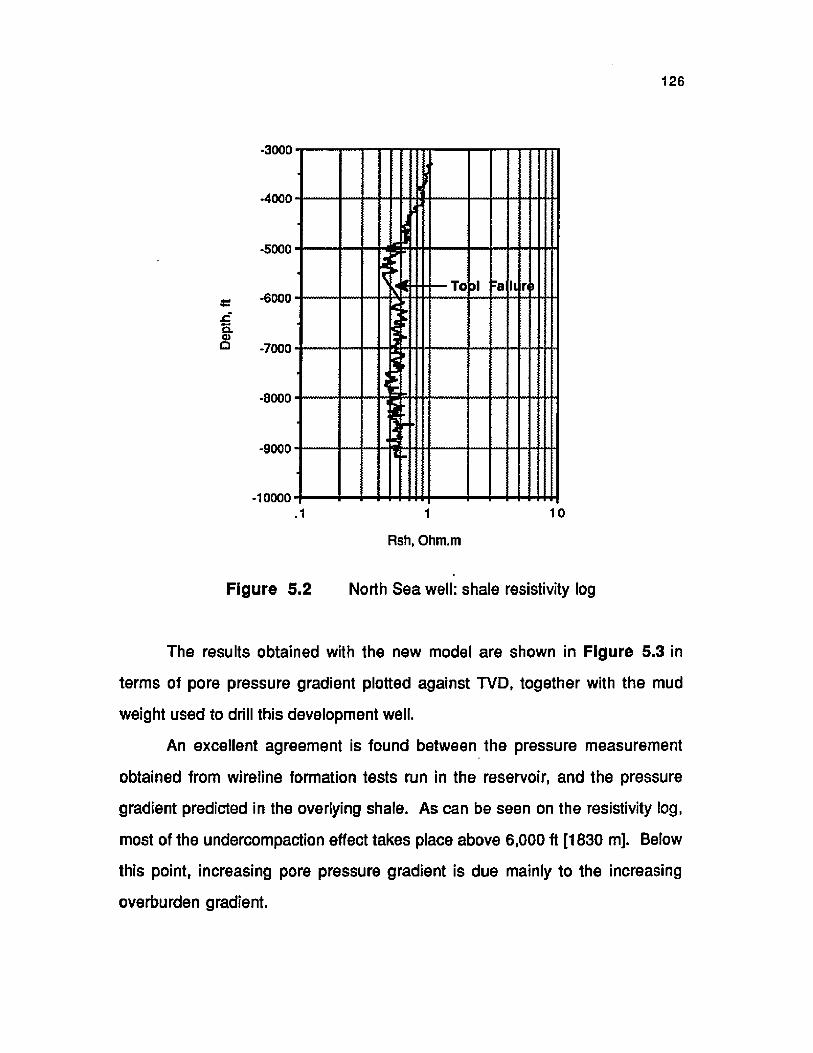
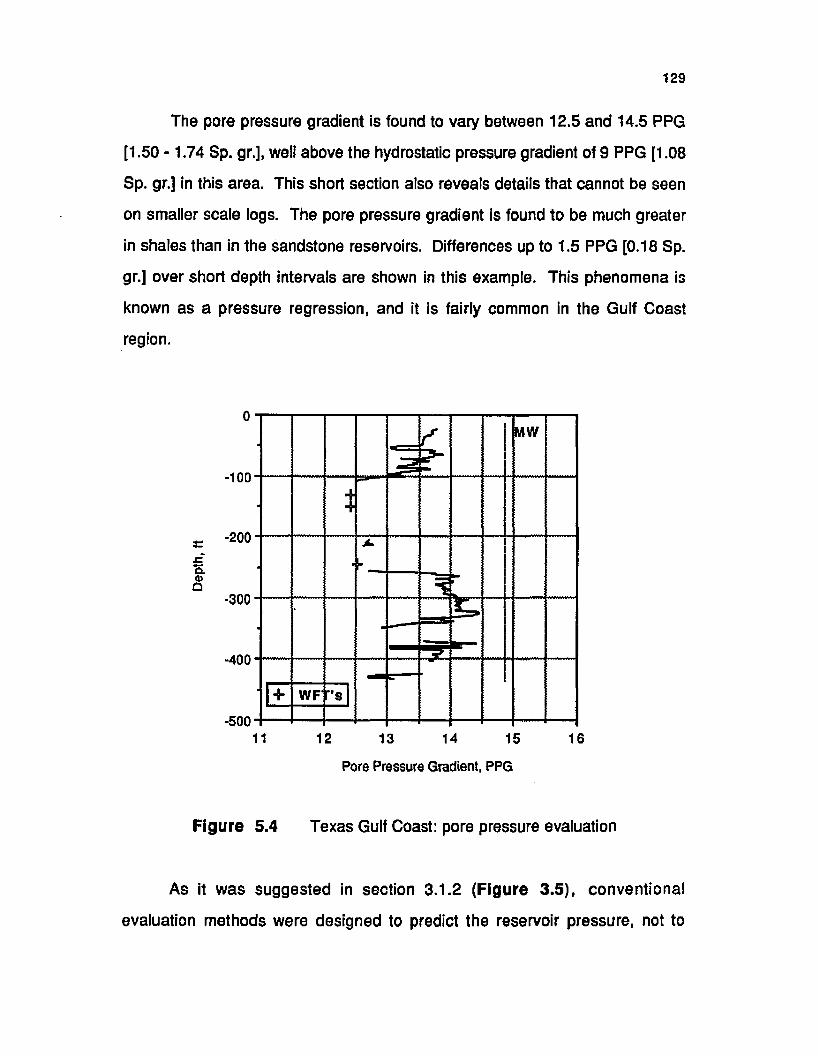
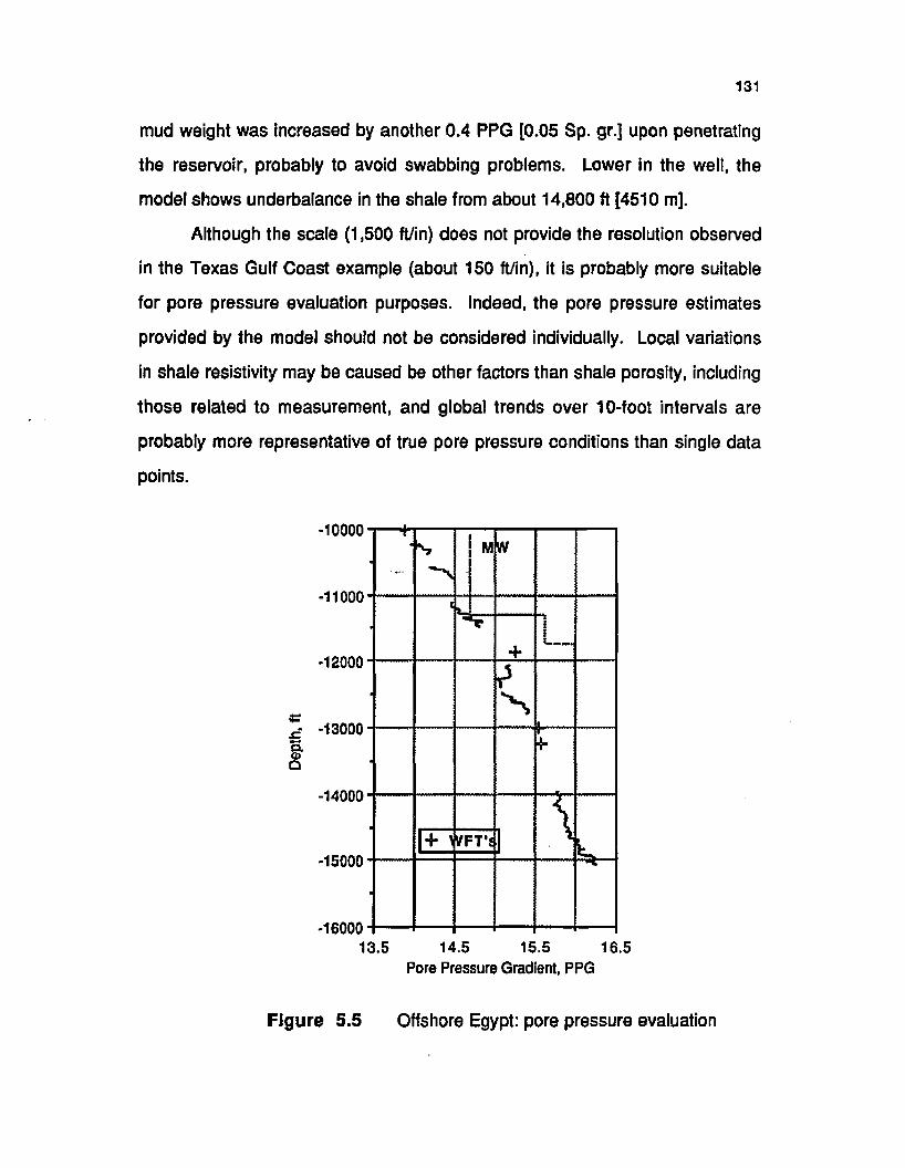
straight line over a limited stress range.4.19 116 Summary of equations.5.1 121 Summary of useful equations in their numerical format.5.2 126 North Sea well: shale resistivity log.5.3 127 North Sea well: pore pressure evaluation.5.4 129 Texas Gulf Coast: pore pressure evaluation.5.5 131 Offshore Egypt: pore pressure evaluation.5.6 133 Louisiana Gulf Coast: drilling history.5.7 134 Louisiana Gulf Coast: pore pressure evaluation.6.1 138 Schematic of disposal well.6.2 140 Permeability vs effective stress correlation [Clark, 1988].

xi

Figure Page

6.3 142 Porosity/Permeability correlation for a sandstone sampleduring mechanical loading [LeRoy and LeRoy, 1977].

6.4 144 Rebound/recompression phenomena associated to thepermeability-effective stress relationship and intercept

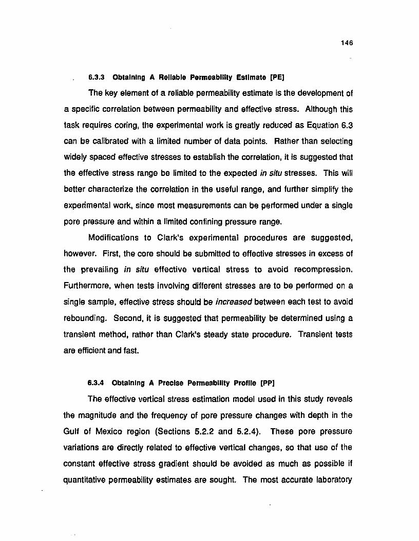
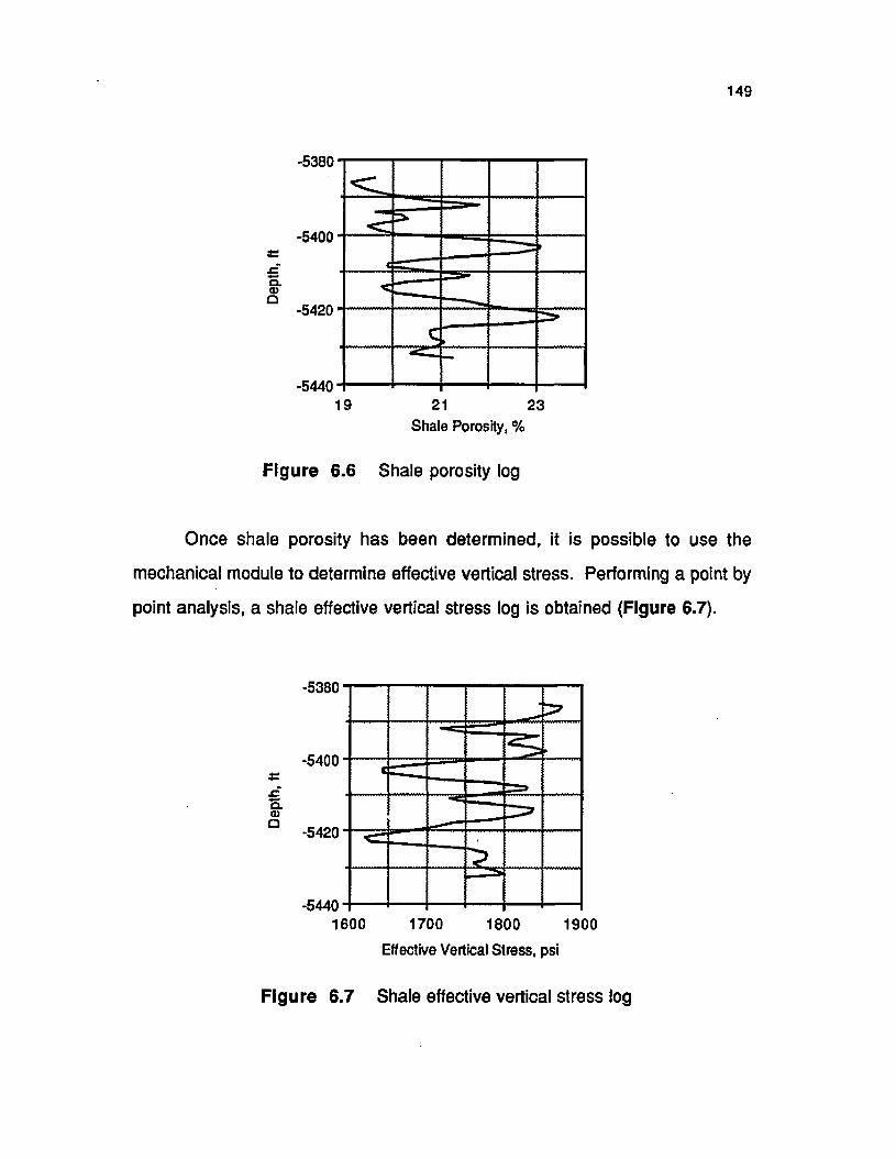
variations.6.5 148 Shale resistivity log.6.6 149 Shale porosity log.6.7 149 Shale effective stress log.6.8 150 Shale permeability log.6.9 151 Pore pressure log.A.1 170 Sphere placed in a uniform and constant electric field.A.2 173 Spherical coordinates.A.3 186 Generalization of the potential equation.B.1 196 An elementary volume element in cylindrical coordinates.B.2 199 Definition of the system.B.3 205 Stress distribution example.B.4 2 0 6 . True skin depth of 2 MHz MWD resistivity tools.

xii

ABSTRACT

In this dissertation, a general method to determine the vertical effective

stress in shales while drilling is developed. The concept is applied to the

development of a model restricted to sodium smectitic shales, which iare

interpreted using Measurement-While-Drilling (MWD) resistivity data. Effective

stress is introduced as the key parameter in the evaluation of petrophysical

properties of shales, which provides a wide range of applications to the method.

The model comprises two interpretation modules: an electrical module

converts shale resistivity into porosity using a new formation factor relationship

adapted from previous work, and a mechanical module relates porosity to void

ratio using the one-dimensional compression theory. This approach eliminates

the use of normal trends and allows a true real-time interpretation. Most of the

advantages of the new model relative to conventional techniques result from the

modular approach, which also leaves room for future improvements. In

particular, the electrical module can be replaced by any other algorithm capable

of providing shale porosity. Two applications are described.

The first application allows the real-time evaluation of pore pressure,

which is obtained from effective vertical stress using Terzaghi's relationship.

The model lends itself particularly well to field implementation. It proved

extremely versatile in a variety of drilling environments, including exploration

drilling, and more accurate than conventional methods during field tests.

xiii

The second application provides in situ shale permeability estimates

using correlations between permeability and effective stress. A new

experimental procedure is suggested to develop such correlations.

The effective stress concept appeared to be a powerful interpretation tool

in the study of shales, and iti's suggested that generalized "effective stress logs"

be developed and used routinely in the evaluation of saturated porous media.

CHAPTER I

INTRODUCTION

1.1 NORMAL PORE PRESSURE

The fluids contained in porous subsurface formatio.ns generate stresses

due to the pressure they exert on their environment. This pressure is known as

pore pressure. If the pore pressure is caused by the hydrostatic head of

connate water only and there is pore-to-pore communication up to the

atmosphere, pore pressure is qualified as normal.

The pressure gradient of a normally pressured zone is thus only

dependent on connate water density, which is primarily a function of its

chemical composition. Temperature and pressure may also affect connate

water density through compressibility. In practice, however, changes in connate

water density with depth are not taken into account, and a constant hydrostatic

gradient is used over the entire depth range of interest. These normal pore

pressure gradients are associated to Equivalent Water Densities (EWD) ranging

from 1 g/cm3 (0.433 psi/ft) for fresh water to 1.074 g/cm3 (0.465 psi/ft) for salt

water, as shown in Table 1.1.

Therefore, the notion of normal pressure is not universal. Rather, it

appears to be area-dependent. The knowledge of local conditions (i.e. EWD) is

thus necessary to determine whether a formation is normally pressured or not.

1

2

Pressure Gradient Equivalent Water Density psi/ft g/cm3

West Texas 0.433 1.000Gulf of Mexico Coastline 0.465 1.074North Sea 0.452 1.044Malaysia 0.442 1.021Mackenzie Delta 0.442 1.021West Africa 0.442 1.021Anadarko Basin 0.433 1.000Rocky Mountains 0.436 1.007California 0.439 1.014

Table 1.1 Normal formation pressure gradients for several areas of active

drilling [Bourgoyne et al, 1986]

1.2 ABNORMAL PORE PRESSURE

Any formation fluid pressure which does not conform with the definition

given above is "not normal." Current terminology actually distinguishes

between pressures lower than normal (subnormal), and pressures higher

than normal (a b n o rm a l); the latter are also called "overpressures" or

"geopressures." Note that in this definition, "abnormal" refers to the magnitude

of the pore pressure relative to what normal pressure should be at a given

depth. The occurrence of geopressures, however, is not "abnormal," as shown

in Chapter II.

Distinguishing between normally and not normally pressured formations

seems rather straightforward: knowledge of connate water density and

formation pressure at a given depth should be sufficient. In practice this is

rarely true, and at least one more parameter must be known: the source.

3

1.3 THE SOURCE AND PRESSURE GRADIENT CALCULATIONS

Additional difficulties in the definition of the pressure regime of a

formation arise from the use of average pressure gradients calculated from an

arbitrary reference point, as represented by Equation 1.1.a:

G = PpD - PpD, D - D r

Where: Ga is average pore pressure gradient

D is current depth

Dr is the reference depth

Ppz is pore pressure at depth z

For practical purposes, the depth reference is usually taken at the Rotary

Table Kelly Bushing (RTKB). This choice, however, rarely suits pressure

gradient calculations because at least two fluids of distinct densities are present

between the point of interest and the reference point: connate water and air. In

general, the depth reference should be taken at the source, where contact is

established between formation fluid and atmosphere. Offshore, the source

corresponds to the Mean Sea Level (MSL). Onshore, the level of the water

table must be determined. In some instances, the source may be several

hundred feet deep. In other cases, particularly in mountainous terrain, the

source may be higher than the RTKB.

Regardless of these important calculation technicalities, two apparent

pressure regimes may actually be observed by the drilling crew, depending on

the relative vertical position of the wellsite and the source:

4

1. If the wellsite is higher than the source, pore pressure should be

atmospheric until the water table is reached and hydrostatic from that

point (Figures 1.1.a, 1.1 .b). To the drilling personnel, however, pore

pressure will appear less than hydrostatic.

2. Conversely, if the well is lower than the source, pore pressure will

appear higher than normal. Artesian wells are a good example of this

situation (Figure 1.1 .c).

These apparent pore pressure anomalies are due to the relative position

of the wellhead and the source. In both cases, pore pressure is actually normal,

i.e. caused by the hydrostatic head of connate water. Correct selection of the

depth reference (i.e. at the source} usually allows the discrimination between

apparent and actual pressure anomalies. However, selecting the source as the

depth reference is not always justified, particularly when hydrodynamic

phenomena are involved. In such non-static cases, pressure drop calculations

must be undertaken to determine the equivalent source level. A much simpler

approach to resolve the ambiguity consists in using the true pressure gradient

of the formation fluid, given by:

Where: Gt is true pressure gradient as a function of depth

D is depth

Pp is pore pressure as a function of depth

5

Ppore= atmospheric pressure

ioop-

S O D '

o J w ater tab

point at which reservoir reaches surface (the source)

F igure 1 .1 .a The wellsite is higher than the source and the fluid- bearing formation is hit above the water table

source

pore-l -W,

o -i

H u =height o f thew ater column between the source level and the top o f the reservoir in the well

Ww = average w ater density

F igure 1.1 .b The wellsite is higher than the source and the fluid- bearing formation is hit below the water table

source

F igure 1.1 .c The wellsite is lower than the source

Figure 1.1 The source concept [CSRPPGN, 1981]

6

In practical applications, pore pressure is not known as a continuous

function of depth. Local pressure gradients are then best suited to describe

pore pressure changes with depth. Local gradients can be determined using

Equation 1.1.a repeatedly over depth intervals of limited extent and

independently of a fixed depth reference. Equation 1.1.a becomes:

Where: [Dji D ^ ] is the ith depth interval

G|. is the local pressure gradient of the ith depth interval

Pp. is pressure at depth D[

Shorter intervals allow the local gradient to be closer to the true pressure

gradient, hence it becomes more representative of actual pore pressure

regimes. Use of Equation 1.1 .b, however, is limited by the number of pressure

measurements available and their vertical spacing.

1.4 SCOPE AND CONTENT OF THE DISSERTATION

During drilling operations, mud weight must be adjusted to meet several

requirements. One is to prevent fluid influx into the wellbore by raising mud

weight, although excessive mud weight may cause fracturing of the formation.

Without considering this extreme case, a high pressure differential between the

wellbore drilling fluid and the formation fluid will reduce the penetration rate and

thus increase drilling cost, as explained in Chapter III. Because mud weighing

7

is a costly operation, unnecessary high mud weights should be avoided.

Mud weight cannot be optimized to satisfy these requirements unless the

pore pressure regimes encountered by the wellbore are known as drilling

progresses. Moreover, pore pressure gradient changes with depth are a

relatively common occurrence in a single wellbore; so that, mud weight

optimization while drilling is a dynamic process, not a one-time operation.

Because mud weight adjustment is so critical to the safety and efficiency of

drilling operations, the drilling industry has devoted over 25 years of continuous

research in an effort to develop a reliable pore pressure evaluation method.

Unfortunately, due to the complexity of the problem, a final answer has not been

attained, and research is still in progress.

The main difficulty in pore pressure evaluation while drilling is that a

direct pressure measurement is impossible. Indeed, no tool is available that

can be incorporated to the Bottom Hole Assembly (BHA) and perform direct

pore pressure measurements. One of the reasons such a tool has not been

designed is the frequent association of overpressures with shales, as explained

in Chapter II. Due to their extremely low permeabilities, shales do not allow the

practical performance of conventional pressure tests. The driving idea is to infer

pore pressure by interpreting pressure-dependent parameters that can be

measured.

Normal and abnormal regimes are encountered in the drilling of oil and

gas wells, but abnormal pressures cause the principal threat. The purpose of

this study is to detect and evaluate abnormal pressures where the average

formation fluid gradient is greater than hydrostatic. However, the theory

8

developed herein could very well be expanded to detect and evaluate

subnormal pressures.

To identify the pressure-sensitive parameters of interest in the evaluation

of abnormal pressures, it is necessary to understand the mechanisms

responsible for the generation of overpressures, and to determine the effect

they have had on the subsurface environment. Only then is it possible to relate

the measurable modifications caused by these mechanisms to the magnitude of

the overpressures they have resulted in.

This general approach calls for a review of the causes of overpressures.

Chapter II presents the main mechanisms documented in the literature during

the last 25 years and summarizes current knowledge in this area. Chapter III

then introduces the pore pressure evaluation concepts in use since the early

sixties and puts them in their historical perspective. Also included is a survey of

the options available to the industry at this time, with emphasis on the methods

bearing a real-time potential.

The conclusions drawn at the end of Chapters II and III combined with a

survey of the available Measurement-While-Drilling (MWD) technology set the

basis for the development of a new interpretation model. The effective stress

concept is discussed in Chapter IV, providing a logical lead to the philosophy of

the proposed model, whose theoretical foundations are also exposed. The

result is a shale effective vertical stress evaluation method.

In Chapter V, the real-time capability of the model is exploited to provide

pore pressure estimates while drilling using MWD resistivity logs. Four field

examples are analyzed and discussed, thus allowing a direct evaluation of the

model's performance. At the same time, it is clearly shown that the approach

lends itself to field implementation.

By offering a second application to the determination of effective vertical

stress in shales, Chapter VI enhances the possibilities of the effective stress

principle and sets new grounds for future research in the area of petrophysics.

A method to estimate in situ shale permeability is proposed, and the results

obtained suggest a new approach to evaluate the sealing properties of shale

layers.

Finally, Chapter VII summarizes the results of this research, formulates

conclusions and recommendations, and speculates about future developments.

CHAPTER II

OVERPRESSURE GENERATION MECHANISMS

Considerable disagreement exists among earth scientists concerning the

mechanisms responsible for generating abnormally high pore pressures.

Numerous processes have been proposed in the past to explain the occurrence

of geopressures, but very few were unanimously accepted. This chapter

reviews the less controversial overpressure generation mechanisms and

attempts to settle some of the arguments by incorporating the results of recent

studies. As expected, however, this effort is far from putting an end to the

discussion, which remains open.

Abnormal pore pressure generation mechanisms are thus not fully

understood. Despite the speculation that characterizes their study, the literature

systematically refers to a very small number of processes considered effective

in developing overpressures. These are:

□ Differential density effect

□ Compaction disequilibrium of argillaceous sediments

□ Tectonic activity

□ Shale chemical diagenesis

□ Aquathermal pressuring

10

11

The presence of abnormal pressures in many sedimentary basins

around the world is usually attributed to one of these processes with variable

levels of confidence. The differential density effect is clearly effective in creating

abnormal pressure situations in hydrocarbon-bearing reservoirs, as shown in

section 2.1. Compaction disequilibrium of argillaceous sediments is the most

widely accepted model in young tertiary sedimentary basins. All abnormal

pressure evaluation methods developed up to now are based on this model,

which is discussed extensively in section 2.2. Tectonic activity also has the

potential to generate overpressures over wide areas. In contrast, aquathermal

pressuring and shale chemical diagenesis are associated to a much greater

degree of uncertainty as to their ability to generate overpressures. Other

mechanisms appear marginal when compared to these five principal causes.

The following sections provide insight on each of these mechanisms.

The conclusions drawn from this analytical review will provide the principles of

abnormal pore pressure detection and evaluation techniques described in the

next chapter.

2.1 DIFFERENTIAL DENSITY EFFECT

The natural pressure gradient of a fluid is a function of its density. The

true pressure gradient is lower in a hydrocarbon-bearing zone than it is in a

water zone because hydrocarbons have lower densities than connate water.

This effect increases as the difference in density between connate water and

hydrocarbon increases. It is therefore particularly significant in gas-bearing

formations.

12

Consider a gas-bearing formation whose closure is h, limited at the top

by a caprock at depth Dc, and at the bottom by water at depth (Dc+h) (Figure

2.1). Even though the water at the Gas Water Contact (GWC) and above the

caprock may be hydrostatic, the gas reservoir will be abnormally pressured.

Let Ppz be pore pressure at depth z,

PHz be hydrostatic pressure at depth z,

G|g be the local gas pressure gradient,

Ghw be the connate water hydrostatic gradient.

At any depth z in the reservoir, the overpressure, APpz, is the difference

between reservoir and hydrostatic pressures:

APpz= Ppz ■ Phz

APpz = [GHw ■ (Dc + h) - G|g . (Dc + h - z)] - G^w. z

APpz = (G|g + GHw) • (Dc + h) + (Gjg - GHvv) . z

and APpD(j= (GHw-G |g ).h

At the caprock, the gas-bearing formation is overpressured by an amount

which is a function of the closure and the difference between the water and gas

local pressure gradients. The average pressure gradient at the top of the

reservoir is greater than at the GWC, and a higher mud weight will be required

to drill the top of the gas zone than deeper into it. Table 2.1 summarizes the

results which were obtained with the following numerical values:

h =3000 ft G|g =0 .0416 psi/ft (0.8 PPG)

Dc = 5000 ft Ghw = 0.465 psi/ft (9 PPG)

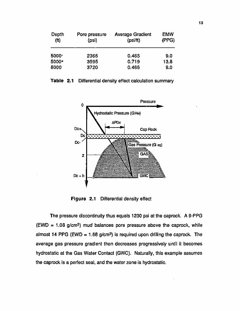
Depth Pore pressure Average Gradient EMW (ft) (psi) (psi/ft) (PPG)

5000- 2365 0.465 9.05000+ 3595 0.719 13.88000 3720 0.465 9.0

Table 2.1 Differential density effect calculation summary

Pressure0

Dc-k^ Dc

DC- ^

Z

Dc + h

Figure 2.1 Differential density effect

The pressure discontinuity thus equals 1230 psi at the caprock. A 9-PPG

(EWD = 1.08 g/cm3) mud balances pore pressure above the caprock, while

almost 14 PPG (EWD = 1.68 g/cm3) is required upon drilling the caprock. The

average gas pressure gradient then decreases progressively until it becomes

hydrostatic at the Gas Water Contact (GWC). Naturally, this example assumes

the caprock is a perfect seal, and the water zone is hydrostatic.

Hydrostatic Pressure (GHw)

Gas Pressure (G ag)

14

2.2 COMPACTION DISEQUILIBRIUM OF ARGILLACEOUS SEDIMENTS

2.2.1 Compaction Disequilibrium

Overburden is the stress created at depth by overlying sediments.

Overburden thus finds its origin in the weight of the solid matrix of the porous

medium and the saturating pore fluid. That portion of overburden due to solids

is termed "lithostatic pressure." By definition, it is related to overburden and

hydrostatic pressure by Equation 2.1:

2v = Xs + Ph (2,1)

Where: £ v is overburden pressure

Xs is lithostatic pressure

PH is hydrostatic pressure

As sediments settle at the bottom of the sea, interstitial water and

seawater form a continuous phase; so that, pore pressure is essentially

hydrostatic (Figure 2.2.a). At this stage, pore pressure results from the weight

of the overlying fluid only, and there is no stress transfer from the solid phase to

the liquid phase. Since pore pressure is hydrostatic, Equation 2.1 actually

describes the stress distribution between the two phases.

As sedimentation progresses, vertical stresses increase progressively in

response to the constantly increasing overburden. Provided the matrix is

somewhat compressible, the additional load will cause deformations of the

porous medium that will tend to reduce the pore volume. In the absence of a

pore fluid, these deformations would result in a porosity reduction only, but the

15

presence of a compressible fluid complicates the process. The pore fluid

opposes the deformation, which increases pore pressure. At this moment, a

new stress distribution prevails. Not only does the pore fluid bear the

hydrostatic pressure, but it also supports part of the lithostatic load. A stress

transfer has thus occurred between the two phases. While Equation 2.1 is still

valid, it loses its physical meaning. The new stress distribution between the two

phases is now represented by Equation 2.2:

Zv = [JW- 5P ] + Pp (2-2)

Where: l v is overburden pressure

A.s is lithostatic pressure

Pp is pore pressure

5P is the portion of lithostatic pressure transferred to the fluid

Note that:

5P = Pp - Ph (2.3)

5P is the amount of overpressure of the pore fluid relative to hydrostatic

conditions. The fluid is more compressible than the solid porous structure that

contains it. Thus, the deformation of the porous rock proceeds until a balance

between overburden, the increased pore pressure, and that part of the

lithostatic pressure actually sustained by the solids is attained.

The pressure excess supported by the fluid phase generates a pressure

potential which drives some of the fluid out of the pore space towards areas of

16

lower pressure potential. This causes further porosity reduction until a new

hydrostatic equilibrium is reached (Figure 2.2.b). As long as fluid How is not

prevented, sedimentation is compensated at depth by compaction resulting in

the following phenomena:

□ Porosity decreases as depth increases

□ Pore pressure remains hydrostatic

□ The shale compacts "normally"

The continuous pressure adjustment characteristic of the sedimentation

process can be visualized as a close succession of metastable equilibria. Each

equilibrium results from a delicate balance between:

□ The rate of stress increase due to sedimentation

□ The matrix compressibility

□ The pore fluid mobility

When these parameters allow the fluid to escape at a sufficient rate, the

pore fluid remains hydrostatic until the final stage of compaction (F igure

2.2.c). But if any one of these parameters prevents the system from reaching

hydrostatic equilibrium, the fluid remains overpressured as more sediments

deposit. Typically, conditions favorable to compaction disequilibrium are:

[Cl] High sedimentation rates

[C2] High matrix compressibility

[C3] Low permeability

17

Figure 2.2 The stages of shale compaction m water

□ clay particlesclaystone

E13 shalel:lj%l future reservoir

Figure 2.2.a

Figure 2.2.b

Figure 2.2.C

DEPOSITION: CLAYDuring the initial stage of deposition, interstitial water and seawater form a continuous phase, while water adsorbed by clay minerals prevents direct contact between clay particles. Pore pressure is essentially hydrostatic.

INCREASE IN OVERBURDEN WEIGHT:CLAYSTONESome water is being driven out of the pore spaces as a result of compaction. The clay matrix supports the entire lithostatic load, shale compacts, and pore pressure remains near-hydrostatic.

FINAL COMPACTION: SHALEUnder quasi-equilibrium conditions, pore liuid is allowed to escape progressively during the entire compaction process. Pore pressure remains near hydrostatic throughout the process.

TIME j

18

Local overpressures are generated within the porous medium if the flow

rate of formation fluid is too low to continuously adjust the stress increase

caused by sedimentation. The presence of a permeability barrier, for instance,

is instrumental in preventing the fluid from escaping, thereby favoring a global

pressure build up within the sediment. In addition, by remaining in the porous

rock, the overpressured fluid also prevents further porosity reductions.

Compaction disequilibrium is therefore associated to the following phenomena:

{P ij A slower decrease of porosity with depth

[P2] An increase in pore pressure

[P3] Undercompaction

Conditions favorable to compaction disequilibrium are commonly found

in deltaic depositional environments, where sedimentation rates are high

(condition C1). Shales are the typical formations involved, due to their high

matrix compressibility (condition C2) and their extremely low permeability

(condition C3) which provides unique self-sealing capabilities.

2.2.2 Reservoir Overpressuring Mechanism

Reservoir rocks typically do not have the characteristics necessary to

induce compaction disequilibrium. Due to their greater permeability and lower

compressibility, these rocks are not likely to generate overpressures during

sedimentation, unless the reservoir is perfectly sealed early in the burial history.

This situation is not very common and cannot account for the numerous

overpressured reservoirs encountered in the subsurface.

19

The frequent association of overpressured reservoirs with adjacent

undercompacted shales would suggest that overpressures were generated

within the confining shales and then progressively transmitted to the sealedt- ’

reservoir by fluid flow. Note that in this case, although the reservoir must be

sealed to allow overpressure maintenance, the seal may have been created

much later in the burial history.

The pressure transmission concept from shale to reservoir reveals the

inherent instability of the overpressuring process which is essentially dynamic,

rather than static. Even though sedimentation rate may be greatly reduced

following the compaction disequilibrium phase, the shale system still evolves in

an effort to attain hydrostatic equilibrium. Fluid flow occurs extremely slowly

from the undercompacted shale towards areas of lower fluid potential in order to

restore the pressure equilibrium between the overpressured shale and the

neighboring formations, which were initially hydrostatic.

Depending on the prevailing boundary conditions, fluid flow from the

overpressured shale may occur under two distinct regimes. If the fluid flows

from the shale into a sealed reservoir, the quasi-constant reservoir volume

causes a pressure build-up, and the reservoir becomes overpressured. The

pressure gradient between the shale and the sand is then expected to vary

rather smoothly. If the shale leaks into an open system, however, the boundary

condition is one of constant pressure (hydrostatic), and there is no pressure

build up. Provided permeability remains identical, flow rate is expected to be

greater than in the previous case since the pressure gradient varies much more

abruptly. This passage from hydrostatic to overpressured condition defines the

transition zone.

20

2.3 SHALE CHEMICAL DIAGENESIS

2.3.1 Smectite Utilization And Dewatering

"Diagenesis includes all physical and chemical changes in sediments

that take place after deposition and before metamorphism, excluding

weathering at the Earth's surface," [Eslinger and Pevear, 1988]. The main

physical change during shale diagenesis is due to compaction, whose

overpressure generation potential has already been analyzed (See section

2.2). The dominant diagenetic chemical transformation in shales is the

progressive evolution of smectite into iliite.

Illitization has often been cited as a possible cause of geopressure

[Burst, 1969; Magara, 1975; Bruce, 1984]. However, only the dewatering

reaction of smectites which accompanies illitization may induce overpressures

[Colten-Bradley, 1987], To understand the possible relation between this

process and abnormal pore pressure generation, a brief description of

smectites and the characteristics of their interlayer water is necessary.

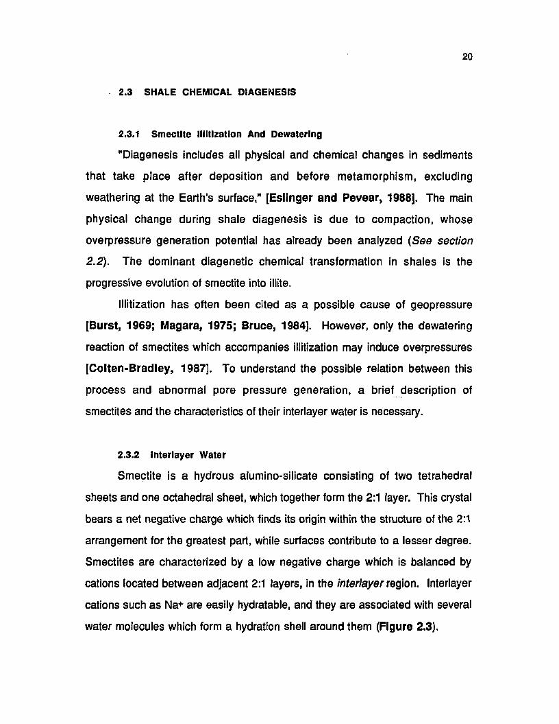
2.3.2 Interlayer Water

Smectite is a hydrous alumino'Silicate consisting of two tetrahedral

sheets and one octahedral sheet, which together form the 2:1 layer. This crystal

bears a net negative charge which finds its origin within the structure of the 2:1

arrangement for the greatest part, while surfaces contribute to a lesser degree.

Smectites are characterized by a low negative charge which is balanced by

cations located between adjacent 2:1 layers, in the interlayer region. Interlayer

cations such as Na+ are easily hydratable, and they are associated with several

water molecules which form a hydration shell around them (Figure 2.3).

21

2:1 Layer

Interiayer Hydrated Cations

Tetrahedral Layer

Octahedral Layer

Tetrahedral LayerNegative Charges

Figure 2.3 2:1 layers and interlayer hydrated cations

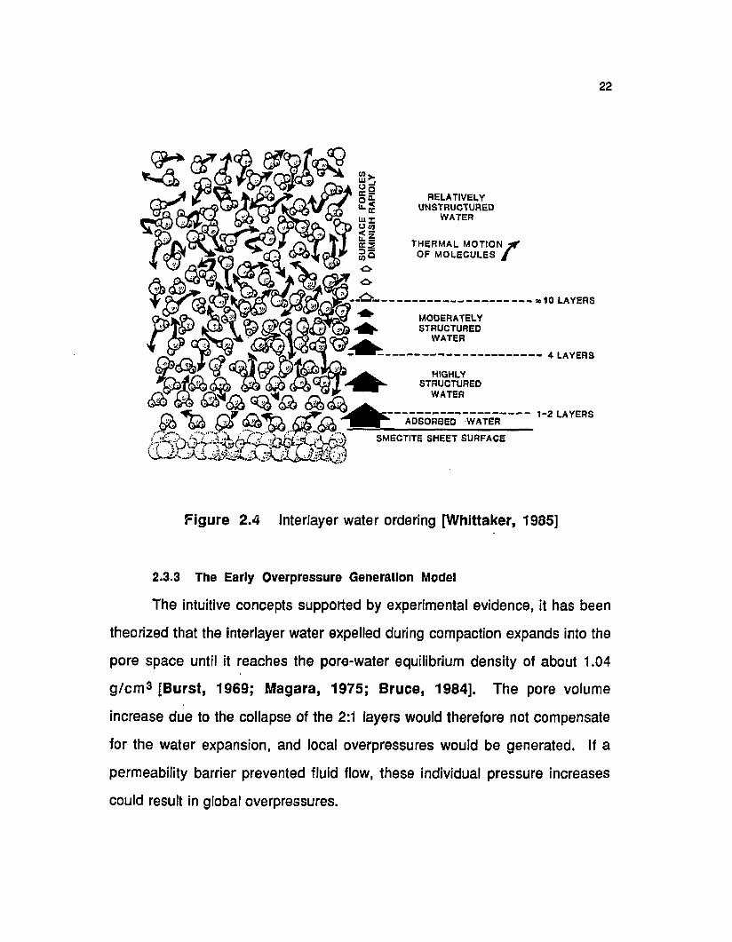
In response to the electrostatic field created by the negative charges of

2:1 layers, the hydrated interlayer cations also develop Van der Waals bonds

with the clay surfaces. When the cation is closer to the surface, a greater

amount of energy is involved, the bond is stronger, and the packing of water

molecules around the clay surface is tighter. Conversely, an increase in

distance from the clay surface is associated with a weakening of the bond. This

schematic description of interlayer particle behavior suggests the concept of a

varying structural order of the interlayer water molecules, as illustrated by

Figure 2.4.

The actual structure of interlayer water is still the object of speculation.

The structure may be different from bulk water. In particular, it was suggested

that the density of tightly bond interlayer water is greater than 1 g/cm3, and

values ranging from 1.27 to 1.41 g/cm3 have been reported [Dewit and

Arens, 1950; Mooney e t al, 1952].

22

IS "E“™EEYC s * uns™ ? ™ ed^ o - \ v 1 w2) JCJ* <5

’ / V T t J E S THERMAL MOTION f f© 4 & '1 © 4 * ' w “ OF MOLECULES /

k?J e S & f i 5 . ^sNenSwv^ Qj A <m .(j|s ° ‘^ r 3 K ^ * 10 la yer s

> ^ 0 ^ ^ MODERATELY

— „ _

( ^ T H I G H L Yn k b f © io c m o & Q structured

< & % m & <*$ * k &- « - w 1-2 LAYERS

' ADSORBED WATER

SMECTITE SHEET SURFACEi>j

Figure 2.4 Interlayer water ordering [Whittaker, 1985]

2.3.3 The Early Overpressure Generation Model

The intuitive concepts supported by experimental evidence, it has been

theorized that the interlayer water expelled during compaction expands into the

pore space until it reaches the pore-water equilibrium density of about 1.04

g /c m 3 [Burst, 1969; M agara, 1975; Bruce, 1984]. The pore volume

increase due to the collapse of the 2:1 layers would therefore not compensate

for the water expansion, and local overpressures would be generated. If a

permeability barrier prevented fluid flow, these individual pressure increases

could result in global overpressures.

23

2.3.4 A Modern Approach

Noting that most of the research on smectite behavior has been

conducted under atmospheric conditions, Colten-Bradley [1987] performed a

thermodynamic study of the dehydration of smectite under high-temperature

and high-pressure. She concluded that "simple dehydration of smectite does

not play a role in the generation of abnormally high fluid pressures,” mainly

because :

1. 2:1 hydrated clays are stable under high-temperature and high-

pressure conditions.

2. Any local increase in pressure would favor rehydration of the clay, or

at least, inhibit further dewatering.

The investigators which initially suggested that shale illitization could

effectively generate abnormal formation pressures had been misled by the

frequently observed correlation between the onset of geopressures and the

increased illite proportion. According to Coiten-Bradley, this association should

be understood differently. By-products of the illitization process include quartz,

kaolinite, feldspars, carbonates, or chlorites. As they precipitate in sandstones

adjacent to shales [M oncure a t at, 1984], they significantly reduce

sandstone permeability. By creating permeability barriers at the top of

sandstone formations, illitization could thus only participate in the maintenance

of overpressures generated by other mechanisms.

24

2.4 AQUATHERMAL PRESSURING

2.4.1 The Model

Following the observation that high-pressure zones are hydrautically

isolated irom their immediate surroundings, Barker [1972] studied the effects of

increasing temperature on the contents of perfectly sealed volumes of saturated

porous rock. Although his theory is based on a Pressure-Temperature-Density

(PTD) diagram, the basic mechanism is essentially similar to the one described

in shale compaction disequilibrium.

Liquids generally expand with increasing temperature, and their

coefficient of thermal expansion under constant pressure is positive:

Where: Cp is the isobaric thermal expansion coefficient of the liquid

T is temperature

P is pressure

V is the volume of the liquid as a function of P and T

An important exception is the case of water, whose specific volume

decreases with increasing temperature upon melting as the ice structure

collapses; but the normal trend of increasing specific volume with temperature

is quickly restored {4 °C @ 1 atm) as the hydrogen bonds responsible for the

anomaly weaken; so that, in the situations of interest to the drilling industry, cp is

indeed positive.

(2.4)

25

Conversely, as pressure increases under constant temperature, liquids

tend to contract. This phenomenon is quantified using the coefficient of

isothermal compressibility, cT, defined to yield positive numerical values:

Where: Cy is the isothermal compressibility coefficient of the liquid

T is temperature

P is pressure

V is the volume of the liquid as a function of P and T

Since temperature and pressure usually both increase with depth, the

effects of thermal expansion and compressibility are opposite. In general, the

effect of compressibility dominates at shallow depths, and thermal expansion

prevails as depth increases. The net effect is then an increase in volume:

dV = cr dP + cp dT (2.6)

dV > 0 (2.7)

The temperature increase associated with burial thus causes the fluid to

expand, thereby initially increasing the local pore pressure. This mechanism is

somewhat similar to the compaction process described earlier (Section 2.2). In

both cases, the fluid flows in response to a local pore pressure increase.

However, increasing overburden causes deformations which ultimately

compress the pore fluid during the compaction process. The fluid now

generates the additional stresses itself in response to a temperature increase.

(2.5)

26

Such self-induced stresses may even cause deformations of the porous

structure. According to this description, the two mechanisms only differ in the

way they generate the initial pressure increase, but the result is identical; so, the

evolution of the system is expected to be similar.

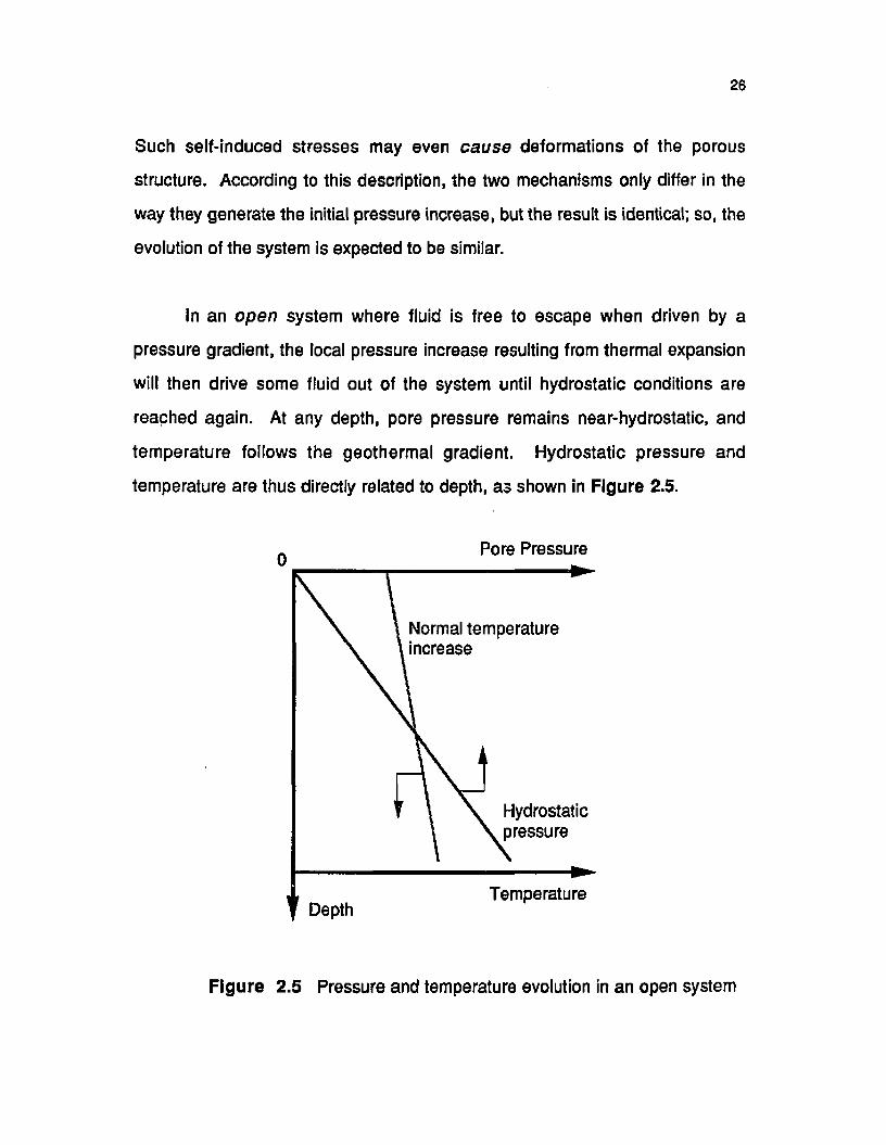
In an open system where fluid is free to escape when driven by a

pressure gradient, the local pressure increase resulting from thermal expansion

will then drive some fluid out of the system until hydrostatic conditions are

reached again. At any depth, pore pressure remains near-hydrostatic, and

temperature follows the geothermal gradient. Hydrostatic pressure and

temperature are thus directly related to depth, as shown in Figure 2.5.

Pore Pressure

Normal temperature increase

Hydrostaticpressure

TemperatureDepth

Figure 2.5 Pressure and temperature evolution in an open system

27

A closed system is expected to behave differently. Assuming no

hydraulic interaction with the surrounding media, Barker [1972] considered the

mass of the sealed system to be constant during burial. He further admitted

pore volume remained constant, and thus concluded that the fluid density is

constant in a sealed system. In this case, the pressure and temperature no

longer follow the trends of Figure 2.5. Instead, the evolution of the two state

variables is determined by the isodensity lines of a PTD diagram (Figure 2.6).

The isodensity lines plotted on the PTD diagram are straight and parallel

lines in the pressure and temperature range of interest. Assuming a constant

pore pressure gradient, pressure and depth are linearly related, so that the

geothermal curve also plots as a straight line in the PTD diagram. It is therefore

possible to determine the value, ©0, of the geothermal gradient which gives a

line parallel to those of the PTD diagram. Barker [1972] found:

©0 = 1 5 °C/km

When the temperature gradient is equal to © „, the pressure and

temperature evolution of open and closed systems are identical. Geothermal

gradients range from approximately 18 °C/km to 55 °C/km, the global average

being 26 °C/km [Selley, 1984]. These geothermal gradients are greater than

0 O; so, the pressure and temperature evolution of closed and open systems are

indeed different. In the general case (0 > 0 O), the pressure increase of a sealed

system is greater than that of an open system for similar temperature changes.

A sealed system would therefore become abnormally pressured by this

mechanism, which Barker [1972] termed aquathermal pressuring.

~ a ® e G<* 0> 3 « -n^ n> p

too0.990 ( t .O t )

98 .02 )

-o

0.909 C l.tO )S 3°°

*n

200

o-

29

2.4.2 Limitations

Barker [1972] pointed out that the thermal expansion of water remains

fairly small. Moreover, Barker [1972] recognized that the phenomenon will be

limited in its magnitude if it occurs in the subsurface, because:

1. Connate water is not pure water, and saline water shows a slower

increase of pressure with temperature along an isodensity line.

2. Unless the "caprock” has a permeability virtually equal to 0 (anhydrite for

example), leakage will always occur and it may be sufficient to annihilate

the effects of aquathermal pressuring [Daines, 1982].

3. Formation volume may increase as a result of increasing pore pressure;

according to Magara [1975], i t "... is not easy to explain geologically,

although there is no physical reason to reject the possibility.”

It was suggested that aquathermal pressuring would be favored within

undercompacted shales where Lewis and Rose [1970] showed that higher

temperature gradients prevailed. Barker [1 9 7 2 ] also theorized that

montmorillonite illitization could provide additional freshwater to a slightly

leaking system, but in view of Colten-Bradley's work [1987, see section 2.3J, it

seems unlikely.

Considering these severe limitations, aquathermal pressuring does not

appear to have the potential to generate overpressures in subsurface

environments.

30

2.5 TECTONIC ACTIVITY

Tectonic activity causes bloc displacements. These displacements

modify the stress pattern in nearby formations which may then become

overpressured. With the exception that additional stresses have different

causes and are applied in a near-horizontal direction, the generation of

geopressures from tectonic compression is again a process extremely similar to

compaction disequilibrium.

As a bloc expands at a given strain rate, it loads neighboring formations

with additional lateral stresses. Provided these formations have a high

compressibility, they will transmit the excess load to the interstitial fluid. The

evolution of the pore pressure will then depend essentially on the relative

values the strain rate of the expanding bloc and the flow rate of the escaping

fluid.

The main difference in the effects of compaction disequilibrium and

tectonic activity is that the former implies a depth increase due to sedimentation,

while the latter can occur without depth change. This apparently minor

distinction has important consequences on the detection of overpressures, as

discussed in section 2.8.2.

2.6 OTHER POSSIBLE CAUSES OF OVERPRESSURES

Other phenomena have been cited in the literature to explain the

generation of abnormal pressures. Most of the proposed processes have been

evaluated on the basis of laboratory experiments or even plain theoretical

considerations, so that their actual contribution to the generation of abnormal

31

pressures in subsurface environments remains to be demonstrated. Osmosis,

for instance, is shown to have the potential of generating pressure differentials

of up to 4500 psi across a semipermeable membrane separating solutions of

1.02 g/cm3 NaCI in water and saturated NaCI bn'ne [Zen and Hanshaw,

1965]. However, Young and Low [1965] showed that because the shales are

highly inefficient semipermeable membranes, osmosis could not be accounted

as a source of overpressure. Fertl [1976] offers a complete review of proposed

overpressure generation mechanisms including some of the more exotic

theories.

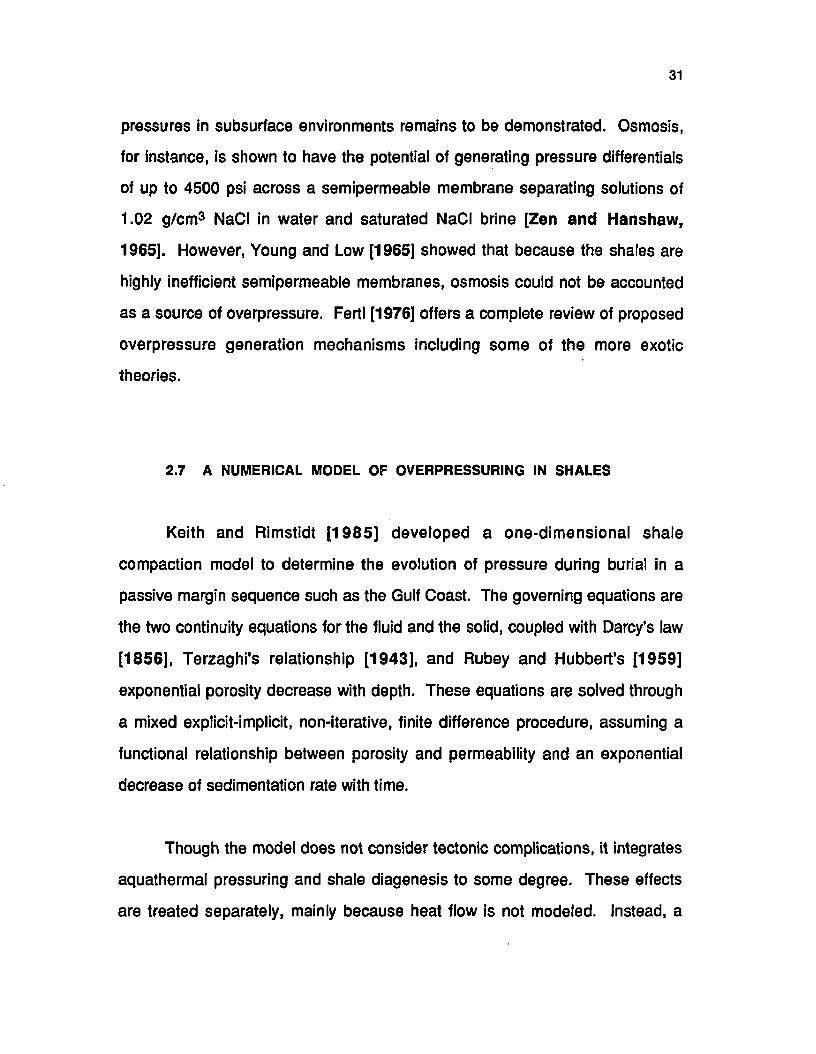
2.7 A NUMERICAL MODEL OF OVERPRESSURING IN SHALES

Keith and Rimstidt [1 9 85 ] developed a one-dimensional shale

compaction model to determine the evolution of pressure during burial in a

passive margin sequence such as the Gulf Coast. The governing equations are

the two continuity equations for the fluid and the solid, coupled with Darcy's law

[1856], Terzaghi's relationship [1943], and Rubey and Hubbert's [1959]

exponential porosity decrease with depth. These equations are solved through

a mixed explicit-implicit, non-iterative, finite difference procedure, assuming a

functional relationship between porosity and permeability and an exponential

decrease of sedimentation rate with time.

Though the model does not consider tectonic complications, it integrates

aquathermal pressuring and shale diagenesis to some degree. These effects

are treated separately, mainly because heat flow is not modeled. Instead, a

32

constant temperature gradient is assumed. The change in porosity resulting

from each process is then simply added to the porosity calculated using the

numerical compaction model.

The results obtained by the authors show that "the effect of thermal

expansion is secondary," and clay dewatering is a "subordinate factor."

Moreover, the magnitude of these effects decreases with time, which leads the

authors to believe that "the major cause of overpressuring in sediments

accumulating along passive margins is nonequilibrium compaction."

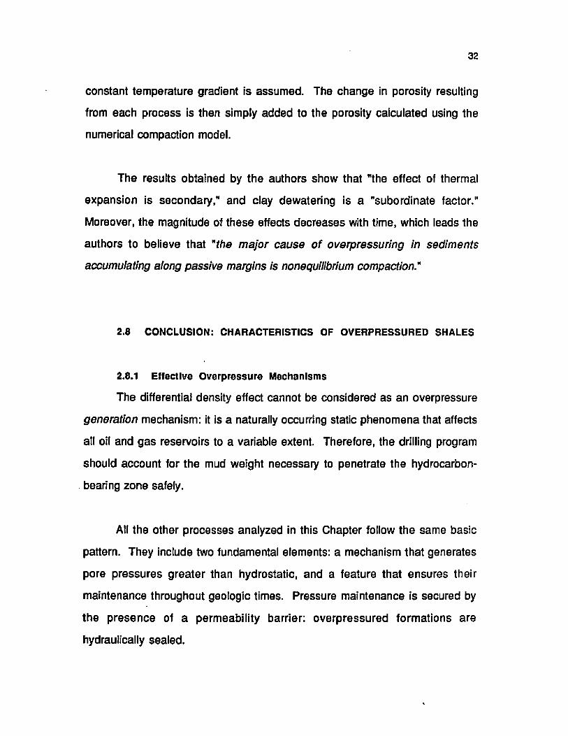
2.8 CONCLUSION: CHARACTERISTICS OF OVERPRESSURED SHALES

2.8.1 Effective Overpressure Mechanisms

The differential density effect cannot be considered as an overpressure

generation mechanism: it is a naturally occurring static phenomena that affects

all oil and gas reservoirs to a variable extent. Therefore, the drilling program

should account for the mud weight necessary to penetrate the hydrocarbon-

bearing zone safely.

All the other processes analyzed in this Chapter follow the same basic

pattern. They include two fundamental elements: a mechanism that generates

pore pressures greater than hydrostatic, and a feature that ensures their

maintenance throughout geologic times. Pressure maintenance is secured by

the presence of a permeability barrier: overpressured formations are

hydraulically sealed.

33

There are basically two possibilities to generate the stresses necessary

to increase pore pressure above hydrostatic in a quasi sealed porous medium:

either fluid volume is increased, or pore volume is decreased. Shale chemical

diagenesis and aquathermal pressuring fall in the first category, while tectonic

activity and compaction disequilibrium correspond to the second possibility.

The present review of the widely accepted overpressure generation

mechanisms reveals that the most effective schemes are those associated with

a porosity reduction process. Moreover, the effectiveness of aquathermal

pressuring and smectite dewatering remains to be demonstrated under

subsurface conditions.

None of the proposed models compare with the ability of compaction

disequilibrium of argillaceous sediments to account for the magnitude of

overpressures and their worldwide occurrence. Abnormal pressures

encountered in the sand/shale sequences are generally associated with

undercompacted shales, especially in deltaic depositionai environments. In

different geological settings, tectonic activity may prove instrumental in

generating overpressures.

Until now, pore pressure evaluation methods were developed assuming

shaie compaction disequilibrium to be the only mechanism effective in

generating overpressures. The present Chapter shows that this assumption is

largely supported by recent experimental and theoretical work. Although

second order processes may be associated, shale undercompaction remains

the main cause of overpressuring in young Tertiary sedimentary basins.

34

2.8.2 Selection Of A Pore Pressure Indicator

The purpose of identifying and analyzing potential overpressure

generation mechanisms is to characterize overpressured environments to allow

their detection and evaluation. Shale compaction disequilibrium is responsible

for most overpressures encountered in young Tertiary sedimentary basins. The

problem of detecting and evaluating overpressured formations is thus

transposed to detecting and evaluating undercompacted shales.

As explained in section 2.2.1, overpressuring during the compaction

process is associated with a slower porosity decrease with depth. The pore

fluid remains in the porous medium instead of escaping; porosity is preserved to

a certain extent. This shale porosity "anomaly" is the key to overpressure

analysis.

All the overpressuring mechanisms described in this Chapter are related

to shale porosity changes. However, because each of these phenomena affect

porosity in a different manner, quantitative analysis cannot be generalized. This

is why it is so critical to determine the cause of overpressures before evaluating,

or even detecting them. An interesting example is that of tectonic activity,

identified earlier in this text (See section 2.5) as a potential source of

geopressures. Whittaker [1 9 8 5 ] reports that "technically produced

geopressures will behave and appear much the same as those resulting from

(vertical) subcompaction." This study also reveals the similarities between the

two processes. However, Whittaker's statement is generally wrong.

The compaction disequilibrium process is associated with a continuous

depth change resulting from constant sedimentation. By maintaining most of its

porosity during burial, the undercompacted interval diverges from the normal

compaction trend towards higher porosity values, in contrast, the tectonic effect

35

is not directly associated to burial: lateral deformation can occur at constant

depth, and the overall effect is then a decrease in porosity, limited in part by the

ability of the formation to retain its pore fluid. Hence, if depth does not come into

play, tectonic effects cause shale porosity departures toward values lower than

the normal trend. The analysis of a porosity log would thus show the formation

to be sub-hydrostatic.

This study is confined to overpressure detection and evaluation in young

Tertiary sedimentary basins, where shale compaction disequilibrium is the most

probable cause of geopressure. In this case, the state of compaction of a shale

is directly related to its porosity, and therefore it characterizes the amount of

overpressure. Unfortunately, shale porosity is not a directly accessible quantity,

and models were developed on the basis of shaie-porosity dependent

parameters rather than porosity itself. Chapter III offers a review of pore

pressure evaluation techniques.

CHAPTER III

PORE PRESSURE EVALUATION OPTIONS

This chapter offers a review of available pore pressure evaluation

methods, it presents the development of two conventional techniques which

have an MWD potential: the resistivity technique and the d-exponent. Methods

based on measurements which are not currently provided by the MWD industry

are not considered in this study. In particular, the interpretation of the sonic

measurement in terms of pore pressures is not addressed, although it may be

one of the most promising techniques. Finally, a review of methods specifically

designed for MWD purposes is also included. This overview of the pore

pressure evaluation options available to the industry will help define the

requirements for the development of a new model.

3.1 PORE PRESSURE EVALUATION USING RESISTIVITY LOGS

3.1.1 Overpressure Detection

The principle of pore pressure evaluation from well logging data is

contributed by Hottmann & Johnson [1965], who first developed a method that

allowed "to infer certain reservoir properties, such as formation pressure, at

any level in the well,” by interpreting "the electrical properties of shales”

36

37

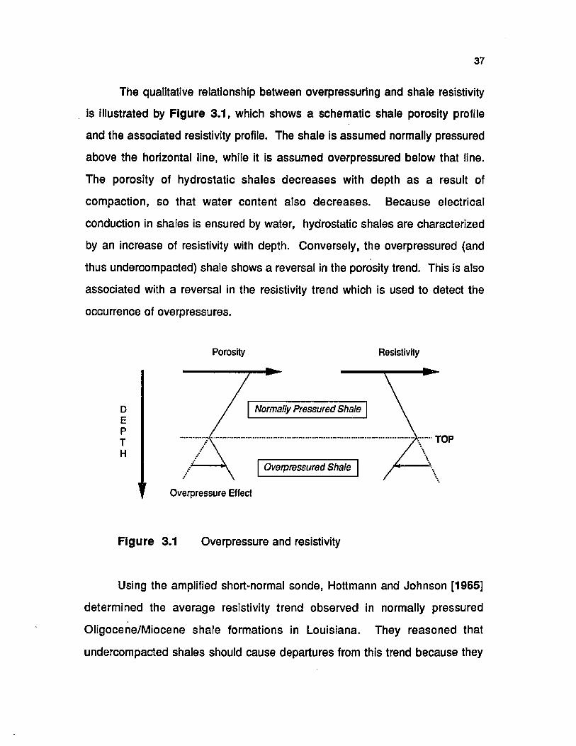
The qualitative relationship between overpressuring and shale resistivity

is illustrated by Figure 3.1, which shows a schematic shale porosity profile

and the associated resistivity profile. The shale is assumed normally pressured

above the horizontal line, while it is assumed overpressured below that line.

The porosity of hydrostatic shales decreases with depth as a result of

compaction, so that water content also decreases. Because electrical

conduction in shales is ensured by water, hydrostatic shales are characterized

by an increase of resistivity with depth. Conversely, the overpressured (and

thus undercompacted) shale shows a reversal in the porosity trend. This is also

associated with a reversal in the resistivity trend which is used to detect the

occurrence of overpressures.

Porosity Resistivity

DEPTH

Normally Pressured Shale

TOP

Overpressured Shale

Overpressure Effect

Figure 3.1 Overpressure and resistivity

Using the amplified short-normal sonde, Hottmann and Johnson [1965]

determined the average resistivity trend observed in normally pressured

Oligocene/Miocene shale formations in Louisiana. They reasoned that

undercompacted shales should cause departures from this trend because they

38

are less resistive than hydrostatic shales buried at the same depth (Figure

3.1 ).

This qualitative, almost intuitive observation is associated to substantial

resistivity changes. Figure 3.2 is a typical shale resistivity log: the upper

resistivity data, obtained in the normally-pressured shale, define the "normal

trend." The sudden shift towards lower resistivity values characterizes the top of

the overpressured shale interval.

-4000

Normal ' Trend

-6000 -

-8000 -Normatly Pressured Shale

S- -10000TOP

- 12000 -

Overpressured Shale

-14000-

-160000.3 0.4 0.5 0.6 0.7 0.8 0.9 1.0

Shale Resistivity, Ohm.m

Figure 3 .2 Overpressures cause shale resistivity to

depart from the normal trend

39

3.1.2 Empirical Evaluation Of Pore Pressure Magnitude

Hottmann and Johnson [1965] developed a correlation directly between

the resistivity departure from the normal trend and the observed fluid pressure

gradient. Resistivity departure is represented by the resistivity ratio:

Where: Rr is the resistivity ratio at depth D

Rsh is the shale resistivity at depth D

Rshn is the normal shale resistivity at depth D

Normal shale resistivity is the hypothetical resistivity of the shale had it

been normally pressured. It is obtained by extrapolating the normal trend line to

the depth of interest (Figure 3.3).

(3.1)

Resistivity

D

Normal Trend Line

Rsh

f Depth

Figure 3.3 Normal resistivity

40

The empirical correlation relates the shale resistivity ratio to the average

pressure gradient (Figure 3.4).

0.90

0.805tnQ.<D 0.70Q.LL

s£ 0.60tno>cc

0.50

0.401.0 2.0 3.0 4.0

Resistivity Ratio

Figure 3.4 Hottmann and Johnson's [1965] resistivity correlation

Since pressure measurements cannot be performed in shales, Hottmann

and Johnson [1965] used the average pressure gradient determined in nearby

sands. Hence, pressure and resistivity data do not originate from the same

depth, and they are not representative of the same lithology. Three different

environments are in fact gathered in Hottmann and Johnson's correlation

(Figure 3.5):

□ Normally pressured shales, where the normal resistivity trend is

defined.

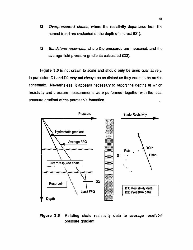
□ Overpressured shales, where the resistivity departures from the

normal trend are evaluated at the depth of interest (D1).

□ Sandstone reservoirs, where the pressures are measured, and the

average fluid pressure gradients calculated (D2).

Figure 3.5 is not drawn to scale and should only be used qualitatively.

In particular, D1 and D2 may not always be as distant as they seem to be on the

schematic. Nevertheless, it appears necessary to report the depths at which

resistivity and pressure measurements were performed, together with the local

pressure gradient of the permeable formation.

Pressure

Hydrostatic gradient

Average FPG

Overpressured shale

'SSSSfSS/fSSSSSSSi'S/Z/y/SSSS/S/yz/SSf/S/S/A

Reservoir D2

Local FPG

y Depth

Shale Resistivity

RshD1

\A TOP\

— \ Rshn

D1: Resistivity data D2: Pressure data

Figure 3.5 Relating shale resistivity data to average reservoir

pressure gradient

42

The authors realized that the resistivity of shale depends on many other

factors than porosity. They identified the following as the most important ones:

□ Temperature

□ Salinity of the contained fluid

□ Mineral composition

However, Hottmann and Johnson [1965] did not attempt to isolate the

effect of each factor, and they assumed the resistivity variations to be due to

porosity effects only. When using an empirical correlation, this assumption may

not be as penalizing as it may seem.

An empirical correlation is essentially a statistical technique. Provided

the data set is large enough to be representative of the area of interest, it can be

considered globally representative of porosity effects and any additional

phenomena. Pressure estimates are thus still possible with reasonable

accuracy in similar horizons, where secondary effects remain of comparable

magnitude. In fact, a regional correlation based on a large number of pressure

measurements is probably the best pressure prediction tool in an area of limited

extension. Conversely, insufficient or non-representative data become a major

source of error. As suggested by Hottmann and Johnson [1965], the

correlation "should be considered as a guide until actual pressure and log data

are obtained for the particular region under study."

A major shortcoming of the method, however, is its inability to estimate

pressure in shales. Unless it is proven that the average pressure gradient is

identical in overpressured shales and in sandstones, the pressure

43

measurements performed in sandstones should not be used to estimate pore

pressure in shale. Although it is a logical consequence of the combination of

data used to establish the correlation (Figure 3.5), this drawback has rarely

been discussed, if ever at all. As it is theorized in Chapter V, this could explain

some of the borehole stability problems encountered while drilling shales.

3.1.3 Theoretical Interpretation

The effective stress concept is analyzed in greater detail in Chapter IV.

At this time, it is simply defined using Terzaghi's [1943] relationship:

cy = - Pp (3.2)

Where: o„ is effective vertical stress

2 V is overburden stress

pp is pore pressure

Based on data published by Athy [1930] concerning bulk densities of a

large number of samples of Mid-Continent shales, Hubbert and Rubey [1959]

found a relationship between shale porosity and effective vertical stress:

<I> = a>j exp(-K av) (3.3)

Where: O is the shale porosity at depth D

<t>i is the shale porosity at surface

K is a constant

ov is the effective overburden pressure

44

The existence of a relationship between shale porosity and effective

vertical stress allowed Foster and Whalen [1966] to develop the equivalent

depth concept. Knowledge of this relationship led them to develop a theory

explaining the empirical correlation obtained by Hottmann and Johnson [1965].

The equivalent depth principle simply states that if the same porosity is

observed in the same formation at two different depths, the effective stresses

must be equal at both levels, as illustrated by Figure 3.6.

<60 Porosity

DN

DA

cN= oA= cA’

DA’

* Depth

Figure 3.6 The equivalent depth principle

Overburden can be estimated from density logs, which allows evaluating

effective vertical stress in the normally-pressured shale shale (point N), where

pore pressure is also known:

45

<*vN = SvN “ PpN (3.4)

Pore pressure is unknown in the abnormally-pressured shale (point A),

but effective vertical stress is equal to ovN ($ A = C>N), and overburden is again

derived from a density log. Thus:

Using the equivalent depth concept thus requires that shale porosity be

known. Foster and Whalen [1966] proposed to calculate shale porosity from

resistivity logs using Archie's [1942] formation factor:

Where: F is the formation factor

Rsh is the electrical resistivity of shale saturated with water

RWSh is the electrical resistivity of the water saturating the shale

While RSh can be obtained from a resistivity measurement, interpretation

methods could not derive RWSh- Foster and Whalen [1966] thus assumed that

the resistivity of the water saturating the shales was equal to the resistivity of the

water saturating the nearest sandstone:

PpA — ^vA " ^vN (3.5)

(3.6)

Rw(nearby sand)(3.7)

Archie's [1942] equation is then used to obtain porosity:

46

Where F is the porosity

m is the cementation exponent (usually 2)

Mathematical manipulations eventually led to the following expression of

the average pore pressure gradient in shales:

^ = 0.465 D + £303 . Log10 (3.9)D Km I Rshf

Although this equation exclusively refers to a shale environment, it helps

explain Hottmann and Johnson's [1965] empirical correlation between average

pore pressure gradient in reservoirs and resistivity ratio in adjacent shales.

3.1.4 The Variable Overburden Gradient

Eaton [1972] was concerned with the scatter observed by Hottmann and

Johnson [1965] in the data they collected. He thought this could be explained

by considering the local changes in overburden gradient and proposed

relationships taking into account these changes for all common pore pressure

detection methods: resistivity, sonic, and d-exponent.

Considering Terzaghi's [1943] effective stress relationship (Equation

3.2), Eaton pointed out that knowledge of the actual overburden stress was

essential to obtain reliable pore pressure estimates using this equation. And

indeed, the overburden stress gradient does vary from region to region; more

importantly, it also varies with depth within the same region. This phenomena is

47

a direct consequence of the compaction mechanism: as porosity decreases, the

bulk density of the porous media increases. Figure 3.7 shows several

overburden gradient curves available in the literature. In the case of the Gulf

Coast, it can be seen that the average overburden gradient hardly reaches 1

psi/ft at depths greater than 20,000 ft and that the average value is in the range

of 0.9 psi/ft. Still, a 1 psi/ft value is commonly used in pore pressure

calculations, thus systematically leading to underestimated pore pressures.

o

- 10

12

1 * Constant Gradient 1.0 psi/ft2 = Texas and Louisiana, U.S.A.,

Gulf Coast Area3 = California, U.S.A., Santa

Barbara Channel4 - North Sea Area

0.7 0.8 0.9 1.0O verburden Pressure G rad ien t, psi/ft

F igure 3.7 Overburden data for several areas [Bourgoyne et al, 1986]

48

The approach Eaton [1972] used is similar to that of previous authors,

but he went one step further and recognized the pressure evaluation equation

as an application of Terzaghi's [1943] effective stress concept. Terzaghi’s

relationship (3.2) can be written in terms of stress gradients. Solving for the

pore pressure gradient:

Eaton [1972] developed an empirical relationship "by trial-and-error

fitting of data, and it predicts the abnormal pressure behavior data of Hottmann

and Johnson fairly well."

This equation is:

fp = L l . Q.535 /Qbserved RshV 5 ,3 .,^D D I Normal Rsh ) 1 ;

In Equation 3.11, the effective stress gradient is represented by the last

term, equal to 0.535 psi/ft (1-0.465, where 1 psi/ft is the assumed constant

overburden gradient, and 0.465 psi/ft the normal pore pressure gradient) in

normally-pressured zones where the resistivity ratio is equal to 1. In fact, Eaton

[1975] realized that in order to account for overburden gradient changes with

depth, the normal effective stress gradient should really be calculated at each

depth as:

IsA - h . . £ e |\ D / n D \ D ) n

(3.12)

49

Finally:

fp - S t . f e j L . (p p | | (Observed RshV 5D “ D \ D I d U I Normal Rsh J 1 ' *

This equation was evaluated with the data published by Lane and

Macpherson [1974]. Eaton [1975] found that a better fit was obtained with a

1.2 exponent on the resistivity ratio. Finally:

This equation is certainly the most widely used in the industry when

evaluating formation pressures from resistivity logs.

3.1.5 Conclusion

Resistivity methods are based on the assumption that overpressures are

the result of shale undercompaction. Qualitatively, these methods perform

relatively well, though difficulties in determining the normal resistivity trend

when little regional experience is available may affect the reliability of

overpressure detection. Interfering factors such as water salinity or clay

mineralogy changes may also bias the interpretation, these side effects

becoming critical during quantitative analysis.

P p _ 2 v [2^ |Pp) [/Observed RSh)1 2 D D " ID ' I d U I Normal Rsh /

(3.14)

50

3.2 PORE PRESSURE EVALUATION USING DRILLING DATA

Considerable experimental work was carried out in drilling during the

late fifties and early sixties, primarily on microbit drilling machines. All

investigators emphasized the major effect of formation pressure a n d

bottomhole pressure on drilling performance. However, due to the diversity and

complexity of the phenomena involved, only qualitative conclusions were

drawn, and the effect of pore pressure itself was not clearly isolated.

In 1966, Jorden and Shirley introduced the d-exponent method,

designed to allow real-time pore pressure estimation while drilling by analyzing

drilling data. This semi-empirical technique was initially developed for soft type

roller cone bits used in the Texas-Louisiana Gulf Coast, but it was soon

successfully applied to many other areas of the world.

The rate of penetration normalization proposed by Jorden and Shirley

[1966] was subsequently improved [Rehm and McClendon, 1971] to take

into account the effect of mud weight and bit wear. Several similar attempts

based on different drilling equations or even empirical correlations were also

proposed. These methods were generally adapted to particular environments

or drilling conditions, where the d-exponent did not perform satisfactorily

[Com bs, 1968; Bourgoyne and Young, 1974; B ellotti and Giacca,

1978].

Interpretation of drilling data is not considered a real-time method at this

stage, particularly when it is based on surface measurements of Weight On Bit

(WOB) and torque. Additionally, as it is explained in Chapter IV, conventional

drilling data interpretation methods such as the d-exponent cannot be

combined efficiently with MWD technology.

51

3.2.1 Rate Of Penetration And Pore Pressure

"Mechanical" pore pressure prediction methods proceed very much like

log-based techniques: the objective is to determine pore pressure using a

measurable pressure-sensitive parameter. Obtaining pore pressure estimates

using drilling performance data, however, appears a difficult task, because

several factors that are difficult to quantify act simultaneously:

[F1] The differentia! pressure factor

[F2] The rock strength factor

[F3J The porosity factor

[ F i ] It is generally agreed that increasing differential pressure between the

borehole and the formation fluid causes a chip hold-down effect,

preventing efficient cuttings removal and causing the bit to re-drill the

cuttings [G arnler and Van Lingen, 1959]. In addition, the same

authors identified a second direct effect of differential pressure: the bit

balling effect. This phenomena results in cuttings sticking to the cutting

surface of the bit, which delays cuttings removal, but will more particularly

diminish the drilling action of the bit. Both effects increase with decreasing

permeability, thus being particularly effective in shales, where they reduce

the drilling efficiency, and consequently the rate of penetration.

[F2] An increasing pore pressure under constant overburden causes an

effective stress decrease (Equation 3.2). Rock strength thus decreases,

which means that other variables remaining constant, ROP increases with

pore pressure. Several authors have also observed that rock

52

strengthening occurs with increasing confining pressure, and suggested

that increasing hydrostatic pressure due to the mud column could also

result in rock strengthening [Cunningham and Eenik, 1959].

[F3] When the cause of overpressuring is compaction disequilibrium, shales

are undercompacted. Independently of the pore pressure effect, the

strength of undercompacted shales is tower than normal due to their

relatively high porosities [Bourgoyne et al, 1986]. This important effect

is rarely accounted for.

Pore pressure thus affects drilling rate via several phenomena, either

directly (porosity effect, rock strength effect), or indirectly through the differential

pressure at the bottom of the hole (bit cleaning, bit balling, and rock strength

effects). In addition, rock strength varies with the pressure exerted by the mud

column. The effect of pressure differential is thus fairly complex and difficult to

isolate. Nevertheless, several pore pressure evaluation techniques based on

drilling performance analysis have been developed, and most of them have

been quite successful.

3.2.2 The d»Exponent

Investigators realized that a relationship existed between pressure and

ROP. However, no definite relation was found between rate of penetration and

differential pressure. Moreover, most of the studies had been performed under

laboratory conditions, while drilling under field conditions seemed not to

respond in a similar manner. Jorden and Shirley [1966] related differential

pressure to ROP and developed a tool to detect overpressures.

53

The theoretical basis for their study was the drilling equation developed

earlier by Bingham [1965] who modeled the rate of penetration of roller cone

bits under laboratory conditions as a function of some of the most significant

drilling variables:

ROP = K RPM WOB (3.15)

ROP is the Rate Of Penetration

RPM is the rotary speed

WOB is the Weight On Bit

D is the bit diameter

K is the rock drillability

d is the WOB exponent

The equation predicts the ROP fairly well as long as WOB, RPM, and bit

size are the only changing parameters. Unfortunately, this is not the case

during field operations, and it was shown that Bingham's equation does not

describe drilling performance under field conditions.

On the basis of this relationship in which the major effect of pressure

differential was assumed to be implicitly included in the WOB exponent (d),

Jorden and Shirley [1966] suggested "that a recognizable relationship

between differential pressure and the d exponent (...) should also obtain under

varying drilling conditions (specifically, varying bit weight, rotary speed, and bit

diameter, with all other drilling variables constant)."

54

If it were possible to hold absolutely all the drilling variables constant, a

simple plot of penetration rate versus depth could be used as a pressure

detection tool. Normalizing the ROP to allow for variations of WOB, RPM, and

bit size, Jorden and Shirley [1966] proposed to plot the d-exponent versus

depth, rather than directly the ROP. In that way, they would filter out the ROP

changes due to WOB, RPM, or bit diameter effects, so that "a plot of d exponent

vs depth should define a trend as the normal pressure section is drilled and the

differential pressure increases. The d-exponent trend should reverse as

overpressured formations are encountered and the differential pressure

decreases-provided all but these three drilling variables are constant." Solving

for d, one obtains:

The expression developed by Jorden and Shirley [1966] is not the

rigorous solution to Bingham's equation. But the authors pointed out that their

intent was to develop an equation for the "Texas Louisiana Gulf Coast, where

there are few significant variations in rock properties other than variations due

to increased compaction with depth." According to them, "ignoring the 'K' term

will not alter the plot of 'normalized1 rate of penetration sufficiently to invalidate

the original premise of the study." Hence, using a drillability of 1 and converting

to field units, Jorden and Shirley [1966] proposed:

(3.16)

12 WOB (lb/1000)(3.17)

55

In field units, the ratio is less than unity. The d-exponent thus60 RPM

varies inversely with the rate of penetration.

The technique developed by Jorden and Shirley [1966] offered an

alternative to pressure detection. The main advantages over log-based

analyses were the real-time capability, and the availability of the necessary data

at the wellsite. But severe limitations restricted the use of this first attempt:

[L i] The method only provides qualitative overpressure detection. It only

applies to undercompacted shale intervals, and further assumes drillability

is constant and equal to 1.

[L2] Bingham's model was developed for soft-formation milled-tooth roller cone

bits actually drilling soft formations, and the use of the d-exponent method

should therefore be restricted to this kind of bits, and certainly not extended

to drag bits or even insert bits or different formations without caution.

[L3] A number of controlling parameters do not appear in Bingham's equation,

such as the effect of hydraulics, or bit wear. These effects are thus

assumed to be implicitly included in the d-exponent as well, whose

variations will therefore not reflect pore pressure changes only.

[L4] Bingham's model is valid only between threshold and flounder point. In

addition, the d-exponent method requires that the ROP actually be

sensitive to differential pressure effects. This is not always the case

[Cunningham and Eenlk, 1959].

56

In view of these limitations, the d-exponent method appeared more as a

pressure detection method, used as a complement to log-based pressure

evaluation method. The d-exponent was generally monitored until it indicated

overpressures; drilling would then be stopped to perform wireline resistivity

measurements and infer the magnitude of the overpressure.

3.2.3 Mud Weight Correction

According to Rehm and McClendon [1971], the differential pressure

effect prevailed over other pressure-related effects. They also realized that

borehole pressure itself was an important parameter controlling the ROP, and

provided an empirical correction to the d-exponent for mud weight changes:

(3.18)

is Shirley and Jorden’s d-exponent

is Rehm and McClendon’s corrected d-exponent

is the hydrostatic gradient

is the Equivalent Circulating Density (ECD) of the mud

being used

This approach allowed the authors to provide absolute pore pressure

estimates, while the work done by Jorden and Shirley [1966] only related the

d-exponent to differential pressure.

The proposed correction is not only important for quantitative evaluation,

it is also critical to qualitative overpressure detection. Because the dcs trend is

better defined, the top of the abnormally pressured zone is easier to detect.

dos=MatLcf05 MW2

Where: d

dCs

MW1

MW2

57

Nevertheless, the same limitations essentially apply to the modified d-

exponent and the d-exponent, except for the fact that the former provides

absolute pressure estimates. The authors stressed the importance of field data

quality for pore pressure estimation applications. They also identified a number

of disturbances created by fluid rheology or drillstring configuration that could

induce rate of penetration variations. An important limitation, however, is added

as a result of the mud weight correction:

[L5] The utility of the modified d-exponent diminishes when the differential

pressure reaches several PPG. Because of the excessive overbalance,

the penetration rate no longer responds significantly to changes in pore

pressure. Under these circumstances, increases in drilling fluid density

will not affect the drilling rate to a great extent, while the corrected d-

exponent will be shifted to lower values which will be interpreted as a

pressure increase. This is unfortunate since it tends to confirm erroneously

the need to increase the drilling fluid density.

The corrected d-exponent proposed by Rehm and McClendon [1971] is

one of the most commonly used in the industry. It has provided good results in

many areas of the world, even though the original d-exponent itself and the mud

weight correction remain questionable. Quantitative interpretation is mostly

performed using Eaton's [1975] relationship:

( fad d I d I d Qbserved dcs

Normal d,Ics i1.2(3.19)

58

3.2.4 Bit Wear Correction

Pore pressure estimation from drilling data requires that the rate of

penetration be corrected for all major variables but pore pressure. Bit wear is

one of these variables which has been modeled to try and normalize the d-

exponent for its effects [G6osevices, 1984]. The basis for the model is a

Galle and Woods' [1963] bit wear correction which was applied to Bingham's

[1965] drilling rate equation:

ROp _ k BEM [WOB.]11aP i D

(3.20)

Where: a is a function of bit wear:

a = 0.93 h2 + 6 h + 1

h _ h[Pt 0.31 hf + 3 hf + 1 (3.22)

(3.21)

h is the fractional tooth wear

hf is the final tooth wear

Dt is the footage at time t

D is the total footage

p=1 for flat-crested wear

p=0.5 for self-sharpening wear

The d-exponent derived from this approach is then given by:

59

Log! of—ELQE— gp d = i !j £Q_BEM

Log10|-12 WOB103 D J

(3.23)

Although bit wear results in a steadily decreasing bit efficiency which

directly impacts drilling performance, it is rarely taken into account, and

Equation 3.18 is generally used.

3.3.5 Other Attempts

Combs [1968], Bourgoyne and Young [1974], and Bellotti and Giacca

[1978] developed pore pressure evaluation methods from different drilling

equations. These three models follow the same general approach: a drilling

equation is developed assuming all variables are independent, and the ROP is

normalized to eliminate the effects of each variable but pore pressure. The idea

is thus similar to the d-exponent; however, these equations attempt to formulate

the effect of pore pressure explicitly, and take more variables into account.

3.2.6 Conclusion

From a theoretical standpoint, the d-exponent should only poorly reflect

pore pressure changes, even when "corrected" for mud density effect. In areas

where transition zones occur over great depth intervals, bit wear becomes

significant and will affect pressure estimates. Practically, however, the d-

exponent has turned out amazingly reliable in undercompacted shale intervals.

The idea of using a drilling model remains interesting. But in order to obtain a

reliable pore pressure estimate, ROP should be explicitly related to other drilling

parameters, including pore pressure. This was done by Bourgoyne and Young

[1974], whose drilling model is probably the most suitable for roller cone bits.

60

PDC bits, however, have received little attention in the area of pressure

prediction. The drilling models available for these tools do not explicitly take

into account pore pressure or differential pressure variations. In field

operations, the d-exponent technique is applied regardless of bit-type, or even

lithology. Due to their simple geometry, kinematics, and drilling action, PDC bits

should be easier to model analytically than roller cones; this should allow the

development of a PDC-specific pore pressure evaluation method. But the

understanding and description of the various effects of pore pressure and

differential pressure on the performance of a drill-bit remain a major difficulty.

3.3 REAL-TIME PORE PRESSURE EVALUATION

The development of MWD technology offered new possibilities in the

area of pore pressure evaluation. No longer delayed by mud logging's lag time,

reliable information concerning drilling mechanics and formation evaluation

became available while drilling. Real-time pore pressure evaluation, however,

required that the data be interpreted on a real-time basis as well.

During the first stage of MWD commercialization, hardware was the

limiting factor in the development of real-time pore pressure evaluation

methods. A good example of this situation is the gamma ray based method

proposed by Zoeller [1983] at the time when no other petrophysical parameter

was available on a real-time basis. When Short Normal (SN) resistivity tools

were introduced, the conventional resistivity technique was implemented into

the real-time environment without any modification. Similarly, when mechanical

61

(WOB and torque) measurements became available, the d-exponent was run

using downhole measurements. Clearly, the industry was not taking advantage

of the real-time capability to its full extent, and the limiting factor shifted to

interpretation, unable to keep up with technological progress.

In the last two years, while this study was in progress, a new generation

of pore pressure evaluation methods has appeared. At the same time, more

reliable sensors have been designed and more measurements are now

available, making real-time pore pressure evaluation a reality. At the same

time, an effort was made to rationalize the theory, although use of empirical

correlations remains current. Nevertheless, apart from the exotic gamma ray

based method, pore pressure evaluation still relies almost exclusively on

resistivity and drilling performance analysis.

3.3.1 Pore Pressure From Gamma Ray Measurements

Zoeller [1983] proposed a method to determine pore pressure from

natural gamma ray measurements. This author theorized that potassium

concentration increases with depth in a normally compacting shale sequence:

according to him, compaction drives water out of the shale system, leaving most

potassium ions behind it. Conversely, undercompacted shale sediments will

retain approximately similar amounts of potassium ions, but the volumetric

concentration of these ions is lower compared to that of normally compacted

shales because of the higher water content.

This qualitative observation was substantiated by empirical quantitative

correlations. First, a normal gamma ray trend line was defined for Gulf Coast

shales (Figure 3.8). Second, departures from this normal trend line are

62

interpreted in terms of pore pressure gradient by use of another correlation

(Figure 3.9). The approach is thus essentially similar to that introduced by

Hottmann and Johnson [1965]. However, while resistivity interpretation is

somewhat supported by theoretical considerations [Foster and Whalen,

1966], an analytical justification of gamma ray interpretation in terms of pore

pressure remains to be developed.

MWO QAMUA RAY. CPS

30 40 00 80100QROUHD LEVEL

1000

3000

K 3000Uftil(L£ 4000HaUJ 8000 Q_ l<(J 8000HaUJ 7000

1113OC 8000

8000

10000

11000

12000

13000

14000

18000

\

N\

i

i

Jo -|Figure 3.8 Normal gamma ray trend [Zoeller, 1983]

63

IDtnaZ 12111

12a<aa 14

111a9-II

01a i*UJ 1T

11

1.11.4 2.0 2.4

— - Q A I tU A HAY PATIO (H O flU A L C P l/C O ltf ttC T E O CP A )

Figure 3.9 Gamma ray pressure correlation [Zoeller, 1983]

3.3.2 Use Of Drilling Data

The Mechanical Efficiency Log (MEL) [Burgess and Lesso, 1985] is a

drilling monitoring tool based on a torque equation for roller cone milled tooth

bits [W arren , 1984] . Using downhole torque and weight on bit

measurements, it provides estimates of bit condition and formation strength.

MEL provides the "rock strength" (RS) of the drilled formation as a

function of drilling variables. Lesso and Burgess [1986] adapted the model to

pore pressure and porosity estimation while drilling. Their interpretation is

based on the value of RS, which they related empirically to formation properties

and differential pressure. According to the authors, this "technique is probably

the most quantitatively reliable real-time method available for formation

evaluation and pore pressure determination while drilling."

64

3.3.3 Use Of Resistivity Measurements

The approach used in recent work is the one developed by Foster and

Whalen [1966] to verify the empirical correlations obtained by Hottmann and

Johnson [1965]. Holbrook and Hauck [1987], and Bryant [1989] have

proposed pore pressure evaluation methods based on a similar scheme. The

difference appears in the correlations used to determine shale porosity and

effective vertical stress.

Holbrook and Hauck [1987] assume two lithologies: sand and shales.

The distribution between the two is determined from the gamma ray reading.

The formation factor is then determined from resistivity measurements using

Waxman and Smits' equation [1968] for shaly sands, although the authors did

not specify how this equation could be used on a real-time basis. Shale

porosity is then obtained using Archie's equation.

Once porosity and lithology are known at a given depth, density is

computed as a weighted average of the matrix and fluid densities, thus allowing

a calculation of overburden. The effective stress is obtained from Rubey and

Hubbert's empirical correlation [1959], which was specifically developed with

Gulf Coast data:

av(D) = tTmax-O'®) (3.24)

Where: gv is the effective vertical stress

Cmax is the stress required to reduce a particular lithology to

zero porosity

O is porosity

65

According to Rubey and Hubbert [1959], a is equal to 6.35. Values for

amax were found to vary between 6,000 psi (shale) and 50,000 psi (sandstone).

Substitution of overburden and effective stress into Terzaghi's relationship

yields pore pressure.

The approach of Bryant [1989] follows the model of Foster and Whalen

[1966] more closely. Shale porosity is obtained using Archie's relationship:

^ - = - 3 - (3.25)Rw <Dm

which yields:

fl> _ exp ln Rw^ ln Rsh (3.26)

In this relationship, Bryant [1989] assumes a is equal to 1, while m takes

a value of 2. Rw is treated as a constant independent of depth. This follows the

assumption of increasing water salinity with depth, from 35,000 mg/l TDS (Total

Dissolved Solids) at surface to a constant value of 80,000 mg/l TDS from 9,000

to 20,000 ft. This assumption implies that Rw ranges between 0.02 to 0.04 £ lm

[Schlumberger, 1988], a narrow enough range to assume Rw constant.

Shale porosity is related to effective stress using Rubey and Hubbert's

[1959] correlation which was verified by Baldwin and Butler [1985]. Bryant,

however, modified the solidity exponent to adjust his overburden correlation:

a v = < w ( 1 -® )7’47 (3-27)

66

Pore pressure is finally obtained using Terzaghi’s relationship in a

somewhat original way. Instead of calculating pore pressure as the difference

between overburden and effective stress, the author makes the following

remark: the average overburden gradient at depth is hardly affected by density

changes in overpressured formations. Hence:

X vn = Syg (3.27)

3.4 CONCLUSION

Operators who need to select a pore pressure evaluation method have

limited options which are defined in terms of hardware and software. Two

measurement principles are available: formation resistivity and drilling

performance. Two distinct techniques are then available for the interpretation of

these measurements: those making use of normal trend lines, and those

recently developed for real-time applications. Overall, four combinations are

possible.

These four fundamental methods have one point in common: the use of

empirical correlations. Conventional methods based on the determination of

normal trend lines draw more heavily on them, but the MWD models also use

empirical correlation to relate shale porosity and effective vertical stress in

particular. Consequently, adapting any of these methods to a new environment

requires large data bases to verify the correlations or build a new one.

and

* vn + Ppn - ^va + Ppa

P pa ~ Ppn + (°v n " ^ v a )

(3.28)

(3.29)

CHAPTER IV

REAL-TIME EFFECTIVE VERTICAL STRESS EVALUATION IN SHALES

The effective vertical stress is introduced as the key parameter in pore

pressure evaluation. After defining the strategy devised to meet the real-time

requirements necessary to achieve pore pressure evaluation while drilling

effectively, this Chapter focuses on the development of a new model allowing

real-time effective vertical stress evaluation in shales. Chapter V then applies

the model to pore pressure evaluation, while Chapter VI presents a method to

estimate shale permeability.

4.1 REAL-TIME REQUIREMENTS

4.1.1 Use Of Normal Trend Lines

All conventional pore pressure evaluation methods make use of normal

trend lines (Chapter III). Numerous authors have emphasized the difficulty of

determining such a normal trend, particularly when regional experience is

limited. Furthermore, defining "the" normal trend is an essentially subjective

task extremely dependent on human judgement. The slope and intercept of this

line varies between operators, and rather than easing the task, experience will

creates additional doubts. Automatization of the normal trend positioning using

regression analysis schemes has had limited success.

67

68

Using normal trend lines on a real-time basis adds a new dimension to

the problem. A final wireline log provides the entire profile on which hydrostatic

and overpressured shales should appear clearly, even though determination of

the exact position of the TOP (Top of OverPressure) and placement of the

normal trend may pose some difficulty. At least, it is possible to identify the data

that should be used to define the normal trend.

When using MWD tools, quantitative interpretation is impossible until the

normal trend can be positioned with a reasonable degree of certainty.

Frequently, this requires that the overpressured zone be penetrated, so that the

hydrostatic shale points can be clearly identified. Clearly, this procedure

significantly reduces the advantage of using a real-time data acquisition system.

This inconvenience may appear insignificant, since pore pressure need not be

evaluated in the hydrostatic interval. But quantifying pore pressures is not the

sole issue.

Prior to the evaluation, the difficulty actually lies in the detection of

overpressures. Since the normal trend is constantly being redefined as

additional data become available; whether the formation is hydrostatic or not

remains uncertain: the detection phase is far more difficult on a real-time basis,

as illustrated by the following resistivity example.

Figure 4.1 shows the MWD resistivity data available at a given time

during drilling. At that time, and assuming there is limited experience in the

area, the normal trend line can be positioned as shown, which places the top of

the overpressured shale interval at about 7600 ft [2300 m]. Additional data

becomes available as drilling progresses, revealing that the early interpretation

is erroneous (Figure 4.2).

69

£O.a>Q

-4000-

-6000 -

-8000-

- 10000 -

- 12000 -

-14000-

-16000

TOP

— i— 1— i— 1— i— '— i— i — i— >— i0.3 0.4 0.5 0.6 0.7 0.8 0.9

Resistivity, Ohm.m

Figure 4.1 Early real-time resistivity interpretation

In fact, the top of the overpressured interval appears to be at 10400 ft

[3200 m]. The mistake could have caused unnecessary mud weight increase or

even premature setting of the casing string.

-4000 -i

-6000 -

-8000-

CL -10000- TOP

- 12000 -

-14000 -

-160000.3 0.4 0.5 0.6 0.7 0.8 0.9

Resistivity, Ohm.m

Figure 4.2 Real-time resistivity interpretation after drilling

into the overpressured zone

70

One may argue that abnormal pore pressure is not performed using a

single pressure indicator, and that other parameters such as drilling rate are

also used to detect overpressures. This is true, although one master method is

generally chosen for quantitative interpretation. More importantly, regardless of

the number of parameters that are monitored and interpreted, safety is the

primary objective, if interpretation of one trusted parameter such as shale

resistivity indicates overpressures, the drilling program will most likely be

altered to prevent any hazardous situation.

This example shows that real-time pore pressure evaluation calls for an

interpretation method which does not make use of normal trend lines. More

generally, the method should allow pore pressure evaluation on the basis of the

data acquired at any given time, without knowledge of data to be obtained.

The benefit of a real-time data acquisition system is not substantial unless

measurements can be interpreted as they are made. Conventional pore

pressure evaluation methods are thus incompatible with MWD technology, and

a real-time interpretation model must therefore be developed.

4.1.2 Selection Of A Real-Time Measurement

The primary objective of this study is to improve real-time pore pressure

evaluation using available technology, rather than to develop a new MWD tool

specifically designed for pore pressure evaluation. Considering the current

status of MWD technology, this study investigates the tool best suited for pore

pressure evaluation.

The "purpose," then, is not purely "academic." Pore pressure evaluation

71

is a daily industrial operation, and the choice of an MWD pore pressure

evaluation measurement should not be exclusively based on technical and

theoretical considerations. Practical factors such as tool availability, usage,

reliability, and cost should also be taken into account.

Another element of importance is the difficulty to introduce new concepts

in the drilling industry and have them accepted. This is usually the result of a

long process which naturally requires extensive experiments and successful

field testing. Regardless of the outcome, time is the key element when it comes

to field implementation. This conservative position is understandable in view of

the stakes at play: after all, despite the limitations that have been pointed out up

to now, conventional interpretation methods perform well* enough to avoid

serious accidents. Although kicks are often experienced, blowouts resulting

from drilling into an overpressured zone are quite rare. No matter how accurate

a new interpretation method may be, it will only be trusted and used if it is

perceived as an improvement over existing methods and if the logic behind the

model makes sense to drilling crews. If not, the wellsite personnel will probably

keep on using overlays rather than the results of a sophisticated but obscure

computer program.

The method developed in this study is based on real-time resistivity

measurements. There are several reasons for this choice:

□ Historical, since resistivity measurements have been used for

pore pressure evaluation for over 25 years. The technique has

been widely documented in the literature and well accepted in the

field.

72

□ Practical, since resistivity tools are now provided worldwide by

most MWD service companies. Other tools such as mechanical

subs are limited in their availability.

O Economical, because operators often include a resistivity sub to

their BHA for formation evaluation purposes. A resistivity-based

pore pressure evaluation method therefore requires no additional

hardware, i.e., no substantial additional cost.

□ Technical, in relation to recent developments in MWD resistivity

technology. Propagation tools provide reliable measurements for

quantitative interpretation often providing wireline quality logs.

Finally, the advent of resistivity devices providing measurements ahead

of the bit will eliminate the time lag characteristic of petrophysical pore pressure

evaluation methods, as opposed to mechanical methods making use of drilling

data. Although these new resistivity tools only allow qualitative interpretation at

this stage [Grupping, Harrell, and Dickinson, 1987], future developments

will certainly provide resistivity measurements with a true real-time feature.

4.1.3 General Strategy

The fundamental assumption that overpressures result from shale

undercompaction is accepted. The objective is thus to use resistivity as a shale

porosity indicator and interpret the measurements in terms of pore pressure with

the following constraints:

73

□ The interpretation must operate in real-time: it must be able to

estimate pore pressure using only available shale resistivity

measurements at any given time. Use of normal trend lines to

detect overpressures is excluded.

□ The model should not require more regional experience than

necessary to drill an exploration well: at that stage, geological

phenomena are understood well enough to assess the causes of

overpressures, if any are expected. Use of empirical correlations

requiring a great deal of regional data is prohibited.

□ The method must lend itself to field implementation without

requiring additional weilsite equipment. Moreover, the

interpretation software must come as an operational package

requiring limited input and modifications from the operator.

The general approach first introduced by Foster and Whalen [1966] and

implemented by Holbrook and Hauck [1987] is adequate for real-time pore

pressure evaluation. In particular, this approach closely follows the reasoning

underlying the undercompaction process and its relation to shale resistivity:

compaction disequilibrium creates overpressures associated to shale porosity

anomalies which affect resistivity measurements. Considering this mechanism

in retrospect, analysis of shale resistivity measurements should lead to shale

porosity estimates, which could then be interpreted in terms of mechanical

stresses. This systematic approach leads logically to the two fundamental

elements that a petrophysical pore pressure evaluation model should comprise:

74

□ A relationship between shale porosity and the selected

petrophysical measurement, and

□ The conversion of shale porosity into stress.

While pore pressure evaluation methods developed according to this

general pattern still depend on empirical correlations [Holbrook and Hauck,

1987; Bryant, 1989], the technique presented here is primarily based on

equations derived analytically. Experimental coefficients are needed; however,

they have physical significance, which provides the user with better control and

possibility to adapt to a variety of environments rapidly: because the physical

laws have been derived in the theoretical part of the model, adapting the model

to a new environment requires limited data. Rather than the development of a

new correlation, the adaptation to specific conditions thus appears as a

calibration.

The method proposed in this study includes two modules: the "Electrical

Module," which aims at providing shale porosity from a shale resistivity

measurement, and the "Mechanical Module," which relates shale porosity to

effective vertical stress. While conventional methods attempted to relate

resistivity ratios directly to pressure gradients, the proposed method uses shale

porosity explicitly as an intermediate variable providing a link between the two

interpretation modules.

75

4.2 THE ELECTRICAL MODULE

Clay particles such as smectites bear a net negative surface charge.

When the particles are placed in an ionic fluid, the negative charges are

balanced by cations present in the solution, which become bound to the clay

surfaces. In saline water, the cations are hydrated, so that the hydration water

molecules are also bound to the clay particles. The aggregates composed of

dry clay minerals and hydrated cations are surrounded by bulk water, or "free”

water molecules. The interaction between these components (clay surfaces,

hydrated cations, and free water) was modeled by Gouy [1910] and Chapman

[1913], who independently proposed a similar model known as the diffuse

double layer theory. It provides a reasonable description of the phenomena

involved in hydrated clay minerals and helps define the system whose electrical

conduction is described in this section.

4.2.1 The Diffuse Double Layer Theory

Section 2.3.2. provides a broad qualitative description of interlayer water

and its relation to the generation of overpressures. In the present section,

interlayer water remains the primary concern, but the motivation is now the

understanding of electrical conduction phenomena. No attempt is made,

however, to quantify these phenomena on a molecular scale. Because the

purpose of this study is to develop a field-applicable technique, the

interpretation model should be as simple as possible, and quantitative

description is limited to macroscopic phenomena. Nevertheless, it is necessary

to understand the molecular processes which govern macroscopic behavior.

76

The bonding of hydrated cations to clay surfaces results from the

electrical potential generated by the negatively-charged clay particles. This

potential attracts cations whose concentration thus increases as distance from a

clay surface decreases. Conversely, the concentration gradient created by this

mechanism generates a diffusion potential which tends to restore the original

concentration throughout the solution: the cations thus tend to diffuse away

from the clay surfaces which attracts them. The two processes acting in

opposite directions, an equilibrium concentration profile such as the one

depicted in Figure 4.3 is eventually established.

Clay | ^ — Diffuse Zone Bulk Water

CationConcentration

Distance

Figure 4.3 Cation distribution in the vicinity of a

clay particle

77

There are two electrically charged layers in this model: the negatively-

charged clay surface, and the positively charged cation "diffuse" zone next to

the clay surface. These together form the "double layer." The thickness of the

Gouy layer depends on such parameters as surface charge of the clay mineral,

salinity of the solution, temperature. Molecules which are not in the Gouy layer

are "free." Stern [1924] refined the Gouy-Chapman mode! by taking into

account the dimensions of the cations which are fixed on the clay surfaces, but

the principle remains identical.

While the above description is fairly representative of colloids, the

description of shales is slightly more complex. Because mechanical stresses

cause clay particles to get closer during the compaction process, shales are

best described by taking into account the interaction between nearby clay

particles. In this case, the electrical potentials created by two adjacent particles

superpose, as illustrated by Figure 4.4. The amount of interlayer water

molecules that remains bound to the clay minerals then depends on the

minimum value taken by the bonding potential in the interlayer region relative to

prevailing counteracting conditions. Counteracting effects can be temperature,

which induces thermal motion of the interlayer particles, or even pressure.

Applying pressure on the clay minerals will generate a pressure potential

tending to squeeze interlayer particles out of the system. Conversely,

increasing pore pressure in the water that may exist outside the interlayer

region tends to maintain the interlayer molecules between the clay platelets.

When the potential at mid-distance between two adjacent particles is too

low to maintain the far water molecules within the interlayer region, these

78

molecules are no longer bound: they are free. When free water molecules are

predominant, interaction between clay platelets ceases, and the system can be

treated as a colloid. The amount of interlayer water bound to clay minerals is

measured in terms of interlayer water layer, where a "water layer" designates a

layer of hydrated cations. These qualitative observations can be quantified

using thermodynamics [Mitchell, 1976]. But again, the purpose of this section

is only to provide a basic description of clay/fluid interaction.

Figure 4.4 Interaction between adjacent clay particles

4.2.2 Compacting Clay Minerals

As clay particles settle at the bottom of the sea, the interstitial water forms

a continuous phase with the sea water. The hydration water molecules are

bound to the interlayer cations and the clay surfaces, while the water molecules

Resulting Potential (P=P1+P2)

iElectricalPotential

Distance

79

unaffected by these bonds remain free. As compaction proceeds and the

sediments are buried deeper, free water is expelled from the system preferably

to bound water, but the amount of bound water changes as temperature and

pressure vary. Assessing the bonding state of the water that remains in the

system during compaction is a key to the description of the electrical behavior of

shales.

Recent theoretical work performed by Colten-Bradley [1987] shows that

smectites are stable as hydrated compounds in the deep subsurface. However,

this stability corresponds to one, two, or three layers of hydrated interlayer

cations only. Table 4.1 summarizes the results obtained by Colten-Bradley in

the two extreme cases studied: clay minerals under pore pressure, such as in

shaly sands, and clay minerals under effective vertical stress, such as in

compacting shales.

Loss Of Layer Pore Pressure Effective Stress

3rd 58°-75°C <60°C2nd 67°-81°C 50°-73°C

1 st (and last) 172°-192°C 130°-178°C

Table 4.1 Loss of interlayer water layers under subsurface

temperature and pressure conditions

In her simulation, Colten-Bradiey used average constant gradients for

temperature and effective stress. Her results are in agreement with the

dehydration process described qualitatively in the previous section: greater

stresses cause interlayer cations to be expelled from the system at lower

80

temperatures. With a pore pressure gradient of 0.465 psi/ft and an effective

stress gradient of 0.535 psi/ft, it appears logical that expulsion temperatures are

greater in "pore pressure" conditions than in "effective stress" environments.

Furthermore, the findings of Colten-Bradley agree with the mechanism for loss

of water in excess of two water layers with simple compaction, as suggested by

Powers [1967].

These results suggest that there are generally less than four layers of

hydrated cations between adjacent 2:1 platelets; so that, the bulk of the

interlayer fluid associated to smectites under subsurface conditions can be

considered bound to the clay minerals. Most of the "free" water is expected to

evacuate the system in the early stages of the compaction history, while flow

paths are still available and the shale bed is not too thick.

Consequently, shales can be schematically visualized as a suspension

of insulating particles in a conductive fluid: the insulating particles are the dry

clay minerals; the conductive fluid is bound water. This is the system whose

electrical behavior must be described to derive porosity from resistivity

measurements.

The next section defines shale porosity and attempts to estimate its order

of magnitude using published data. Following this descriptive phase, the shale

electrical conduction model is introduced in section 4.2.4.

81

4.2.3 Expected Shale Porosity

Porosity is defined in general terms as:

Vt

Where: G> is porosity

Vv is the volume of voids

Vt is the total volume

"Basal spacing" is the distance between identical planes of two adjacent

clay particles. The difference between basal spacing and interlayer spacing is

the thickness of the dry clay mineral (Figure 4.5), which is roughly 10 A

[Lambe, 1958].

Sd — Sb ■ Sj (4.2)

Where: Sj is the interlayer spacing

Sb is the basal spacing

Sd is the thickness of the dry clay mineral

Assuming there is no free water in the system, that no water molecules

are bound to the lateral surfaces of the clay particles, and that clay particles are

in lateral contact with one another, the "volume of voids" is represented by the

interlayer volume, which is filled with bound water. Conversely, the "volume of

solids" corresponds to the volume occupied by the dry clay minerals.

Substituting spacings for volumes in Equation 4.1 yields:

82

(4.3)

Sd

Sbe 0 0 ®

9 ® © © ®a

Figure 4.5 Definition of spacings

Table 4.1 shows that loss of bound-water layers is a discrete process. It

should therefore be associated to discrete variations of the interlayer spacing,

which is confirmed experimentally by interpreting XRD (X-Ray Diffraction)

patterns [Sposito and Prost, 1982]. These experiments provide a direct

evaluation of basal spacing. Figure 4.6 shows the evolution of basal spacing

as a function of the number of layers of interlayer hydrated cations, referred to

as "water layers."

It can be seen that the evolution of basal spacing is not a linear function

of water layers. Rather, the increase in basal spacing associated with the

uptake of a water layer increases with water content. This supports the concept

of a varying order within the interlayer as well as the variation of interlayer water

density (See section 2.3.2, Figure 2.4): Van der Waals bonds are tighter when

hydrated cations are closer to the clay surface. As distance increases, bonds

weaken and the packing is looser.

83

Basal spacing, A

0 1 2 3 Water layers

Figure 4.6 Basal spacing as a function of water layers

[Sposlto and Prost, 1982]

Equation 4.3 can thus be used to estimate shale porosity as a function of

the number of interlayer layers. The results are summarized in Table 4.2.

Although this simplified calculation only provides orders of magnitude, the

results are rather unexpected: a few bound water layers result in relatively high

porosities.

Water Layers Porosity, %

1 202 313 44

Table 4.2 Porosity as a function of water layers: direct calculation using interlayer and basal spacings

84

These estimates can be verified with another calculation technique which

uses the "specific surface" concept. The specific surface of a clay mineral is

defined as the surface area of dry clay minerals per unit mass. Smectite has

both an external and an internal surface area (Figure 4.6).

EXTERNAL SURFACE HB8 INTERNAL SURFACE

Interiayer

2:1 Layer

Interiayer

Figure 4.7 Definition of the specific areas of smectite

Due to their interiayer properties, smectites are characterized by a large

internal surface area. Van Olphen and Fripiat [1979] determined their

approximate specific surfaces:

Internal Surface area

External Surface area

750 m2/g

50 m2/g

85

At be the internal specific area,

Psh be the average density of the shale,

Pd be the density of the dry clay minerals,

Pwb be the average bound water density,

Si be the interlayer spacing.

Consider a mass, m, of shale made of two adjacent rows of 2:1 layers

surrounded by their bound water. The volume of voids is the interlayer volume,

which has a thickness equal to Sj. Each 2:1 layer has two internal surfaces

(Figure 4.7). The cross-sectional area of the interlayer is thus equal to Aj/2.

Using Equation 4.1:

mAsivt

The total volume Vt of the shale is related to its average density by:

X U - n t.v, ■ psh

r?- = Pd (1 -4>)+pw B®Vt

Hence: 0> = [pd (1 - <I>) + Pwb <*>] y Si

Finally:

o =0.5 pd A; S;

1 + 0.5 (pd - pwb) As S|(4.4)

86

This equation can provide shale porosity estimates provided numerical

values are given to the tour variables it includes. Bound water density was

assumed the two extreme values of 1 g/cm3 and 1.4 g/cm3 [See section 2.3.2].

Dry smectite density was taken equal to 2.6 g/cm3. The internal specific area

was taken equal to 750 m2/g [van Olphen and Frfpiat, 1979], while

interlayer spacing was given the values derived from the data set of Sposito

and Prost [1982]. The results obtained are shown in Table 4.3.

Water Layers Porosity, % Porosity, %(PWB = 1 9/cm3) (p w b = 1.4 g/cm3)

1 21.2 21.92 34.5 36.53 52.7 57.3

Table 4.3 Porosity as a function of water layers: calculation using specific areas

Comparing the above shale porosity values with the ones obtained

previously (Table 4.2), it can be seen that the orders of magnitude are

comparable. Second order phenomena are expected to cause additional

variations in shale porosity. In particular, the interlayer spacing for a constant

number of interlayer layers depends on pressure and temperature.

It remains that smectites are expected to have porosities ranging

between 10% and 35% under subsurface pressure and temperature conditions,

where there are between one and two bound water layers in general.

87

4.2.4 Formation Factor Relationship For Shales

The formation factor, F, of a porous media is defined by [Archie, 1942]:

F - f 2 (4.5)rtw

Where: R0 is the electrical resistivity of saturated rock

Rw is the electrical resistivity of the fluid saturating the rock

Formation factor relationships relate the formation factor to formation

porosity. The general form of a formation factor equation is:

F = f(O) (4.6)

Where: $ is the porosity of the porous media

f is a function of porosity dependent on lithology

Archie [1942] developed an empirical formation factor relationship

(Equation 4.7) which is widely used. Table 4.4 summarizes the usual values

assumed by a and m for several rock types.

F = TFT (4-7)<t>

Where: a is the formation factor constant

m is the cementation factor

Formation factor equations have never been proposed for shales, which

reservoirs engineers have little interest in. Models [Waxman and Smits,

88

1968; Clavier et al, 1977] have been developed for shaly sands; however,

they cannot be applied to represent shale behavior. One of the reasons is that

clay particles are under pore pressure conditions in shaly sands. The clay

platelets therefore behave approximately as colloids [See section 4.2.1,

Figure 4.3], and they are associated to bound water and free water, as the

dual-water model emphasizes [Clavier et al, 1977],

Table 4.4 Usual formation factor expressions [Schlumberger, 1987]

It was shown in section 4.2.2 that a single fluid type could be assumed

in compacting smectitic shales; bound water. A new formation factor

relationship must therefore be introduced to represent the electrical behavior of

shales.

This study suggests the use of an equation developed by Perez-Rosales

[1975]. His equation is primarily based on theoretical work by Fricke [1924],

who provided a mathematical treatment of the electrical conductivity of disperse

systems by solving Maxwell's equations for electromagnetism. In the case of

spherical conductive particles placed in a conductive liquid, and for a zero

Equation Application

p _ 0.81 Sands

Compacted Formations, Chalks

Sucrosic Rocks

.2.1 lo 3.0 Oolicastic Rocks

89

charge density, Fricke solved the Laplace equation and obtained:

k .-i JSa.-iki___

k + 2(4.8)

Where: ko is the conductivity of the entire system

k-t is the conductivity of the fluid

k2 is the conductivity of the solid particles

p is the volume concentration of solids

According to the description presented in section 4.2.2, a compacting

shale can be modeled as a suspension of insulating particles (clay platelets) in

a conductive fluid (bound water), and Fricke's modelling suits this description

fairly well. Equation 4.8 could thus be adapted to describe shale conductivity by

substituting zero for the solids' conductivity, k2:

The concentration of suspended solids, p, in Fricke's equation is

analogous to solidity, the complement of porosity, (1 -®). Substituting solidity

for p and writing the equation in terms of resistivities yields:

ko _ ^

(4.9)

f k - i(4.10)

90

Where: R* is the resistivity of the fluid

Ro is the resistivity of the system

$ is porosity

Rearranged, the equation can finally be written:

(4.11)Rw 2 0

This expression of the formation factor derived from Fricke’s work could

be used in this form if a shale could actually be assimilated to a suspension of

non-conductive solids spheres in a conductive fluid. This is not the case,

however, and Equation 4.11 must be modified to represent the geometry of clay

platelets and their high concentration in the "suspension." Perez-Rosales

[1975] adapted Fricke's work to porous media and obtained:

Where: Rq is the resistivity of the system

Rw is the resistivity of the fluid

M is a geometrical factor

<£> is porosity

4>r is residual porosity

(4.12)

M accounts for departures from the ideal spherical shape of the

individual particles, and $ r is the part of the porosity that does not participate

effectively in electrical conduction. Perez-Rosales [1975] found a value of 1.85

91

for M and 0.1 for €>r satisfactory for sand. At this point, specific values for shales

have not been obtained, and the numerical values suggested by Perez-Rosales

[1975] are used. The complete derivation of Equation 4.12 is found in

Appendix A.

In shales, the saturating fluid is bound water, and the equation becomes:

1 + 1 .85 -1 (4.13)Rwb - o.1

Where: Rsh is shale resistivity

Rwb is bound water resistivity

$ is porosity

Archie's [1942] equation (4.7) is sometimes applied to shales [Bryant,

1989]. Figure 4.8 compares Archie’s relationship to the one developed by

Perez-Rosales. It can be seen that for identical values of the formation factor,

the Perez-Rosales formula yields lower porosities.

The enlargement in Figure 4.8 focuses on the porosity range of interest

(See Section 4.2.3, Table 4.2 and Table 4.3). It reveals a 5% pu (porosity

unit) shift between the two relationships. The lower values obtained using the

Perez-Rosales [1975] equation are in better agreement with the discrete

dewatering sequence of smectites [C o lte n -B ra d le y , 1987] and the

preservation of the last interlayer water layer in most occurrences.

192

5 0 -

0 40 -1L L

. 1 3 0 *

25 30 35

Archie: F£ 20 -

Perez-Rosales: F = 1 +1.850 - 0.1

10 30 50 70 90

Porosity, %

Figure 4.8 Comparison of Archie and Perez-Rosales relationships

Use of Equation 4.13 to determine shale porosity requires the knowledge

of the true shale formation factor, The numerator of this ratio is given byRwb

a resistivity measurement, corrected for the usual environmental effects. The

denominator, however, cannot be determined by conventional well logging

interpretation techniques. A typical approach assumes water resistivities in

shales and in a nearby sandstone to be equal [Foster and W halen, 1966.

See section 3 .1 .3\. Bryant [1989] assumed that shale water resistivity is

constant over the depth range of interest.

None of the earlier approaches is representative of shale pore-water as it

has been described in section 4.2.2. This research argues that bound water

provides the electrical path in shales. The next section provides the means to

estimate bound water resistivity.

93

4.2.5 Bound Water Resistivity

Clavier et at [1977] established that bound water resistivity is a

universal parameter for sodium clays which depends only on temperature:

RWB = 0 .1 5 Q .m @ 2 5°C

The effect of temperature, however, was found to be much more

important than for saline solutions.

Earlier pore pressure interpretation models based on resistivity logs did

not need to consider temperature effects because they used resistivity ratios to

determine pressure gradients. When calculating the ratio of observed shale

resistivity to normal shale resistivity at the same depth (as required by Eaton's

method for example) the error was minimal. However, methods making use of

the equivalent depth concept [Foster and W halen , 1966] included

temperature-related errors since they compared resistivities at different depths.

Because the pressure evaluation model proposed in this study makes

use of a single resistivity value (not a ratio), temperature correction is required.

The data published by Clavier et a l [1977] are used to establish a temperature

correction. An excellent curve fit is obtained, as can be seen by plotting the

data points in a log-log coordinate system (Figure 4.9). The relationship

between temperature and conductivity is clearly a power law function:

R W B -P T ^ (4.14)

A least square fit on data of Clavier at at [1977] yields:

Rwb = 297.6 T '1-76 (Temperature in °F)

94

(4.15)

Bound water resistivity can thus be calculated from Equation 4.15

provided formation temperature is known.

EO.CE

#G3280)TS3

3OCD

1000

100

10

1100010010

Temperature, °F

Figure 4.9 Bound water resistivity data [Clavier e ta l, 1977]

Bound water resistivity is not too sensitive to temperature (Figure 4.10):

9RwbBT

= -523.8 T ‘ 276 (4.16)

A general regional temperature gradient profile is usually sufficient to

estimate formation temperature for the pupose of calculating bound water

resistivity. However, bound water resistivity is sufficiently dependent on

temperature for the correction not to be ignored.

95

0.00e+0 ■

U - -1.00e-3-£E

■SZO -2.006-3-0)"s*CO

■s -3.006-3 -

*>‘35Cl

-4.006-3-CL

-5.006-3-

pRwb = - 523,8 T '2,76

1 1— I 1 1— i— | 1--- 1--- r-

60 80 100 120 140 160 180

Temperature, °F

Figure 4.10 Bound water resistivity change with temperature

4.2.6 Determination Of Shale Porosity

Using the shale resistivity measurement and the calcutated bound water

resistivity, the shale formation factor F can be calculated.

p _ R s h

Rwb

Rearranging Equation 4.12 eventually yields shale porosity:

M + <Dr (F -1 )

(4.17)

o =M + ( F - 1)

(4.18)

Using the numerical values suggested by Perez-Rosales [1975]:

Shale porosity can thus be estimated from a single shale resistivity

measurement, and the approximate knowledge of formation temperature. It

should be reminded, however, that deriving shale porosity from resistivity

measurements as shown here is subject to several major limitations.

□ First of all, it is assumed that the Perez-Rosales [1975] equation

provides a reliable description of the conductivity of porous media,

and that it can be adapted to shales (though both coefficients M

and ® r may have to be modified in the future). This is justified on

the basis of the similarities between the description of compacting

clay minerals and Fricke's [1924] modelling.

□ Second, the data presented by Clavier at a l [1977] for sodium

clays are assumed to be representative, and applicable to

overpressured shale environments. This assumption is supported

by the fact that most of the shale water was found to be bound

[C olten-B rad ley, 1987], while Kaiser [1984] has shown that

sodium is the preferred interlayer cation with increasing

temperature.

In addition to these assumptions, which are inherent to the model, it is

also assumed that MWD resistivity tools provide measurements which are

representative of initial in situ conditions. Appendix B studies the mechanical

effects of the borehole within the depth of investigation of 2 MHz resistivity tools.

97

4.3 THE MECHANICAL MODULE

The important long-term forces in rocks arise from gravity and from

contacts between rock systems. Because sedimentary rocks are made of solid

grains and fluid-filled pores, the gross mechanical behavior of porous media

such as shales generally depends on the total stresses (vertical and lateral) and

on pore pressure.

In his study of saturated soils, Terzaghi [1943] introduced the effective

stress concept which solves this double dependency into a single stress type :

the effective stress. The effective stress concept has been brought relatively

early in the area of pore pressure evaluation [Foster and W halen, 1966.

See section 3 .1.3\, but it was not until recently that some of the possibilities of

this powerful concept started being used explicitly [Holbrook and Hauck,

1987; Bryant, 1989. See section 3.3.3].

The effective stress concept is the key to the development of the

mechanical module. More than this, it is the cornerstone of this research, not

only allowing the establishment of a relationship between shale porosity and

prevailing stresses, but also leading to in situ permeability estimates.

This section discusses the effective stress concept and offers a derivation

of Terzaghi's [1943] empirical relationship before presenting the one­

dimensional compression theory which is used to relate porosity and effective

vertical stress.

98

4.3.1 The Effective Stress Concept

The principle of effective stress has been stated by Terzaghi [1943] in

the following terms:

The stresses in any point of a section through a mass of soil can

be computed from the total principal stresses a 1( c2» a 3> which act

in this point. If the voids of the soil are filled with water under a

stress u, the total principal stress consist of two parts. One part, u,

acts in the water and in the solid in every direction with equal

intensity. It is called the neutral stress (or the porewater pressure).

The balance &\ = c\ - u represents an excess over the neutral

stress u, and it has its seat exclusively in the solid phase of the

soil. This fraction of the principal stress will be called the effective

principal stress. (...) A change in the neutral stress u produces

practically no volume change and has practically no influence on

the stress conditions for failure. Porous materials (such as sand,

clay, and concrete) react to a change of u as if they were

incompressible and as if their internal friction were equal to zero.

All the .measurable effects of a change of stress, such as

compression, distortion, and a change of shearing resistance are

exclusively.due to changes in the effective stresses o’i. Hence,

every investigation of the stability of a saturated body of soil

requires the knowledge of both the total and the neutral stresses.

More generally, the effective vertical stress can be defined as the stress

acting in the vertical direction that controls vertical deformations of the porous

media. This definition emphasizes the fact that the effective stress is a

conceptual stress, not a physically measurable quantity. Only its effects,

99

deformations, are measurable. In fact, Terzaghi [1943] obtained the effective

stress relationship empirically, observing during his experimental study that the

deformations of cohesive soils could be attributed to a stress related to applied

load and pore pressure as follows:

<S\ = £j - Pp (4.20)

Where: Cj is effective stress in direction i

£j is applied stress load in direction i

Pp is pore pressure

4.3.2 Derivation Of Terzaghi’s Relationship

Attempts have been made to give effective stress a physical significance.

This has resulted in various terminologies such as "intergranular stressi" or

"matrix stress," being used interchangeably with effective stress. Nevertheless,

the effective stress remains a fictitious quantity, and it should not be associated

with grain-to-grain contact forces, although visualization of the concept can be

useful. The analogy between contact forces and effective stress, however, is

the result of a misconception in the analysis of static equilibrium of porous

media, as it is shown below.

Consider a fictitious horizontal plane (P) across a porous medium

submitted to its in situ stresses. These stresses result from overburden, pore

pressure, and grain-to-grain contact. Equilibrium of the plane is ensured by a

balance of forces which are determined by the stresses and the surface area

they act upon. Figure 4.11 illustrates the balance of forces prevailing across

plane, P, which is expressed by Equation 4.21.

100

Fo

......... ' [

;

Fp Fg

(i)

(II)(P)

Figure 4.11 Force balance in porous media

F0 = Fp+Fg {4.21)

Where: F0 is overburden force

Fp is pore fluid force

Fg is grain-to-grain contact force

The similarity between Equations 4.20 and 4.21 has resulted in the

confusion between contact forces and effective stress. In order to determine the

relationship between the stresses involved in Equation 4.20 and the forces of

Equation 4.21, a rapid analysis of stress distribution in porous media is

necessary.

A cross-section across a porous rock sample reveals both solid grains

and voids. Let A be the area of the exposed rock, Ag be the exposed solid

surface area, and A be the exposed void surface area (Figure 4.12):

j? — (4.22)

101

FLUID

MATRIXfa )

Figure 4.12 Cross-section of porous media

Depending on the area they apply on (a , or j^), several stresses may

be defined. Overburden, for instance, is defined as the weight of overlying

solids and fluids applied over the total surface A. According to this definition,

overburden stress is also a conceptual stress, obtained by averaging the effects

of the weight of both phases over the entire cross-section r .

Sv = ! j . (4.23)A

Where: Z v is the overburden stress

F0 is the overburden force

A is the total cross-section area

Figure 4.13 is an enlargement of part (II) which is depicted in Figure

4.11. It shows a detail of the porous structure that helps visualize the area

where pore pressure and grain-to-grain contact stress actually apply. This

allows to calculate the forces Fp and Fg which are used in the static equilibrium

equation 4.21. The following calculations derive relationships between

stresses and the corresponding forces which allow establishing the stress

counterpart of Equation 4.21.

102

Horizontal projection of a contact area

^ m

m

Contact Areas

Figure 4.13 Porous media geometry and stress distribution

[Fp] On all the parts where fluid is present (porosity), pore pressure exerts its

action, which is always a normal stress. There are thus two components

resulting from pore pressure effect. The first one appears directly in the

fluid "cut" by plane, P:

Fpi = Pp (4.24)

Where: Fp1 is the the partial force resulting from pore pressure

Ay is the exposed void surface area

Pp is pore pressure

The second component of the pore pressure effect appears in the solids

cut by plane, P. These solids being partially immersed in a fluid under

pressure, the surfaces of the solid grains are subject to an isotropic

normal stress which can be assumed constant over the size of a grain.

This stress applies over the entire surface of the immersed grains (g)

except for the contact areas (c), where the fluid is unable to exert its

action. F igure 4.14 depicts one of the grains of F igure 4.13. It is

103

shown isolated from its environment which has been replaced by the

actions it exerts on the grain.

Projection oi the contact area on plane (P)

A contact area

Figure 4.14 Pore pressure distribution on

solid grain surfaces

Fp2 = I PPn.I dS (4.25)

Where: Fp2 is the the partial force resulting from pore pressure action

on solid grains.

Pp is pore pressure

rf is the unit vector indicating the normal to plane (P)

i is the local unit vector defining the normal to the grain

surface

Fp2 = Pp H. I i dS

Fp2 = Pp (-3g - -3c)

(4.26)

(4.27)

104

The total pore pressure effect is thus:

Fp = Fpi + Fp2 (4.28)

Fp = Pp ( -^ + -Sg - $ c ) (4.29)

Where: Pp is pore pressure

% is the surface area of the solids intersected by plane (P)

x v is the surface area of the voids intersected by plane (P)

j?c is the projection on plane (P) of the contact areas

affecting the grains intersected by plane (P)

[Fg] The grain-to-grain contact stresses, fCl only act on the contact areas, but

they have unspecified orientation and magnitude. Their normal

component can nevertheless be represented by an average value

defined by:

Fg = Yen %c = ri ■ ^ fc dS (4.30)

Balancing the forces which represent the action of (I) over (II) and the

reaction of (II) over (I) in the vertical direction, one obtains:

Ey A = Pp ( + flg - i?c) + 'Ytfi 2 (4.31)

V _ p (J*v + A q - A c ) — A c

a YonT(4.32)

105

Equation 4.32 is equivalent to Equation 4.21: it is an expression of force

balance in porous media in terms of stresses. This expression is not unique,

however, since other definitions of the average grain-to-grain contact stress

would have led to a different relationship. Equation 4.30 is only one possible

interpretation, which provides a reasonable physical image of the contact

phenomena. It remains unable, however, to quantify the stresses since the

stress distribution, is unknown.

When the contact area between solids is small compared to other

dimensions f a « & , + stg), Equation 4.32 can be simplified:

f a + #g - ^o) - A (4.33)

— Pp + Yen (4.34)

Equation 4.34 can then be used to determine ycn^- provided overburden

and pore pressure are known. This simplified relationship is analogous to the

effective stress equation proposed by Terzaghi [1943] (Equation 4.20) when

written for the particular case of the vertical axis:

Ov = Iv -P p (E4.20.a)

Equation 4.32, however, is more general and takes the form of the

effective stress relationships derived in the theory of poroelasticity [Blot, 1941].

In this theory, the effective stress takes the general form:

Oy S - CX. Pp (4.35)

106

The poroelastic coefficient a takes values smaller than, or equal to 1

[Roegiers, 1987]. Shales, however, do not behave elastically and cannot be

reliably described using elastic models. However, high pressure tests and

experimental studies of acoustic propagation in shales [Tosaya, 1982]

confirm the validity of Terzaghi’s [1943] original effective stress law, which is

used in the present study. Terzaghi’s stress law being accepted, the question

remains as to how effective stress and shale porosity are related, which calls for

the study of shale compaction.

4.3.3 One-Dlmenslonal Compaction

The analysis of compaction is greatly simplified if it is assumed that

strains occur in the vertical direction only. Such an assumption is reasonable

when the lateral extension of the system is great compared to its vertical

dimension. This is the case of sediment compaction, in which vertical

deformations dominate. The volumetric strain is defined by:

ev = ^ (4.36)Vo

Where: £y is the volumetric strain

V0 is the initial volume of a shale sample

V is the equilibrium volume of the shale sample after

applying the compression load

The total volume of the shale sample is given by:

V = Vv + Vg (E 4.37)

Where: Vv is the volume of voids in the sample

Vg is the volume of solids in the sample

107

Equation 4.36 can thus be written:

C d(Vv + Va) ( I Dmv^+^7 (4'3a)

Where the subscript "o" indicates initial conditions. Assuming the solid

grains (dry clay minerals) are incompressible, the volume change observed in a

shale specimen is solely due to changes in the pore volume:

£v = .. dVv ■■ (4.39)Vvo + Vg0

Ev = v L v (4-40)I9£. + Vyo.Vgo Vgo

Finally:

£v = _ d ^ _ (4.41)1 + 6q

Where the void ratio, e, is defined as the volume of voids divided by the

volume of solids. Porosity and void ratio are related by:

e _ (4.42)1 - O

The coefficient of compressibility for the one-dimensional compaction is

defined as void ratio variation obtained per unit effective stress change:

dov(4.43)

Since an increase in effective vertical stress causes a reduction in void

ratio, the negative sign ensures the coefficient of compressibility will have

positive numerical values. F igure 4 .15 shows the typical relationship

between effective stress and void ratio.

F igure 4.15 Relationship between void ratio and effective

stress for one-dimensional compression of cohesive soils

It can be seen that the coefficient of compressibility is a function of

effective vertical stress. This behavior is characteristic of most cohesive soils

which tend to get stiffer as effective stress increases.

ARecompression

Virgin Compression

Rebound

Effective vertical compression stress, crv

If the effective compression stress is reduced below the maximum value

experienced by the sample, the specimen rebounds and absorbs water. The

portion of the curve labeled "rebound" on Figure 4.15 clearly shows the non­

elastic behavior of shales. If the rebound process is interrupted and the

compression resumed, the coefficient of compressibility assumes another value

and evolves until the stress exceeds the maximum value experienced by the

specimen. At that point, the coefficient of compressibility resumes the value it

had prior to the rebound-recompression cycle and evolves as though the cycle

had not been performed; The void ratio-effective stress relationship

corresponding to stress levels in excess of the maximum past stress

experienced by the soil is called the virgin compression line (Figure 4.15).

Plotting the void ratio-effective vertical stress relationship on a semi-log

graph yields a straight virgin compression curve [Perloff and Baron, 1976]

as shown on Figure 4.16.

RecompressionCD

o’‘■SccTJ

I Virgin CompressionRebound

Effective vertical compression stress, Log ov

Figure 4 .16 Relationship between void ratio and effective

stress for one-dimensional compression of cohesive soils

110

The slope of this line is called the compression index:

Cc = - , tie----- {E 4,44)d[Logio Ov]

The behavior of shale under high effective compression stress is not well

represented by Figure 4.16. If it were, there would be a value of effective

stress for which void ratio equals zero. Increasing effective stress beyond that

value would result in negative values of the void ratio, which has no physical

meaning. In fact, the compression index varies with effective stress as Figure

4.17 shows.

a>o"

Virgin Compression

Effective vertical compression stress, Logov

Figure 4.17 Relationship between void ratio and effective

stress for high stress level one-dimensional compression of shales

Naturally, void ratio still decreases with increasing effective stress, but at

a lesser rate. In the present study, it was assumed that the true virgin

compression curve of shales confined under high effective stresses could be

111

approximated by a straight line over a limited stress range (Figure 4.18).

A Void Ratio

eiVirgin Compression

Effective vertical compression stress, Log ov

Figure 4.18 The virgin compression curve can be

approximated by a straight line over a limited stress range

Integrating Equation 4.44 assuming a constant compression index:

e = - Cc Log-jo av + ej (4.45)

Where: e is void ratio

ov is effective vertical stress

Cc is the average constant compression index

6j is the void ratio corresponding to orv = 1 psi on the straight

line approximation

112

4.3.4 Shale Compression Law

Using Equation 4.45 to determine effective stress from the porosity

estimates provided by the electrical module requires that the calibration

coefficients Cc and e; be determined. The experimental data needed for this

purpose were taken from a borehole stability study performed in the North Sea

[Despax, 1988], during which numerous triaxial tests were conducted on

shale samples obtained from full-size cores. When stresses are expressed in

psi, the following values were obtained for the compression index and the

intercept:

Cc = 1.1

e j« 3.84

Equation 4.45 thus becomes:

e = -1.1 Log™ <*v + 3.84 (4.46)

This equation is valid between 1,100 and 2,300 psi, where it allowed to

reproduce the experimental data with less than 1 % relative error on the void

ratio. Use of the same calibration coefficients outside the specified stress range

was found to produce large errors on void ratio estimates (20% relative error at

700 psi). The 1100-2300 psi stress range covers void ratio between 0.5 and

0.14, which corresponds to a porosity ranging between 33% and 12%. In view

of the data derived in Table 4.2 and Table 4.3, this range should be sufficient

in most instances. If not, compression tests must be performed to determine Cc

and 6j in the stress range of interest.

113

Equation 4.45 approximates the virgin compression curve within a limited

stress range. Using the shale porosity estimates provided by the resistivity

module, this equation can now be used to evaluate the associated effective

vertical stress:

av = 1 0 c ,. (4.47)

With the experimental data:

, - 9 - 3.94O v s l O . - u (4.48)

4.4 SUMMARY AND EXAMPLE

The model developed in this study comprises two modules: an electrical

module and a mechanical module. It is able to provide effective vertical stress

estimates in shales using resistivity measurements and formation temperature.

The equations necessary to the interpretation were derived analytically, until

calibration was needed to adjust the ideal model to the real environment. This

approach provides the user with better control and the possibility to calibrate the

model rapidly in new environments.

4.4.1 Assumptions

The fundamental assumption of this study is that overpressures result

from shale compaction disequilibrium phenomena. Other processes that may

be effective are not accounted for, so that a geological evaluation of the causes

of potential overpressures should be performed prior to attempting pore

114

pressure evaluation. This statement applies to the present model or any other

method based on the same assumption.

Other assumptions were made during the development of the electrical

and mechanical modules. They are:

[E l] The Perez-Rosales formation factor relationship applies to shales

[E 2 ] Overpressured shales are predominantly sodium smectites

[E3] Clavier's bound water resistivity data applies to overpressured

shales

[M i] Terzaghi's effective stress relationship applies to overpressured

shales

[M2] Compaction of sediments is one-dimensional

[M3] The virgin compression curve can be approximated by a straight

line

4.4.2 Procedure

Real-time effective vertical stress evaluation in shales interpreting

resistivity logs according to the new method requires the following steps:

115

1. Select a shale interval (using an MWD Gamma Ray reading for

example), measure shale resistivity, and determine the corrected value

Rsh*

2. Estimate formation temperature at the corresponding vertical depth,

determine bound water resistivity (RwB = p T ' 1f) , and calculate formation

factor

3. Calculate shale porosity convert into void ratio (e= -£ - ) ,M + [F -1 ] 1-4>

and determine the vertical effective stress (av= 10 cc).

Note that this procedure leads to an effective vertical stress estimate

using a single resistivity data, without using normal trend lines or empirical

correlations.

4.4.3 Example

The following example illustrates the use of the method, which appears

relatively simple, considering the complexity of the initial problem. The

calibration coefficients required to obtain numerical values are those suggested

in this chapter [See section 5.1.1 for a summary].

The data used here was taken from a North Sea well. Pore pressure is

calculated at 5000 ft [1524 m], where the temperature was estimated to be 121

°F [49.5 °C], and a resistivity measurement gave Rsh = 0.48 £2.m.

e =

Figure 4.19 Summary of equations

In the electrical module, bound water resistivity must first be determined,

using Equation 4.15:

RWb = 297.6 (121 )’176 = 0.064 Q.m

Knowledge of bound water resistivity and measured shale resistivity is

used to determine the shale formation factor from Equation 4.17:

117

Finally, use of the Perez-Rosales equation (4.19) yields porosity:

_ 1.75 + QJ.X7.5 = o.30 (30%)7.5 + 0.1

This porosity is in agreement with the orders of magnitude predicted in

Table 4.2 and Table 4.3.

□ . Now that shale porosity has been evaluated, the mechanical module

can be used to determine pore pressure. The void ratio is calculated

using Equation 4.42:

This void ratio corresponds to an effective stress given by Equation 4.46:

0.43 - 3.84a v = 10 - 1.1 = 1253 psi

Which is within the specified effective stress range [1100; 2300].

When an entire well is studied, the same procedure is repeated each

time a new shale resistivity data is available, and a shale effective stress log

can be produced.

Pore pressure evaluation can easily be performed once effective vertical

stress is known. Use of Terzaghi's [1943] relationship directly provides pore

pressure given overburden:

118

Pp = Zv - av <4.20.b)

For an overburden pressure of 4570 psi:

Pp = 4 5 70 -1 2 5 3 = 3317 psi

The application of the real-time effective vertical stress evaluation model

to pore pressure evaluation while drilling is presented in Chapter V, which also

provides field verification of the model accuracy.

CHAPTER V

REAL-TIME PORE PRESSURE EVALUATION: FIELD CASES

The effective stress evaluation model was entirely designed to allow

resistivity interpretation on a point-by-point basis. Simplifications were made in

the electrical and mechanical modules to produce a method capable of

performing in the field with limited input and judgement from the operator.

The present chapter shows how the model can be used to fulfill its main

task: the real-time evaluation of pore pressure. The analysis of field data

provides a direct evaluation of the global performance of the model. Four

examples illustrate use of the method and demonstrate its accuracy.

5.1 DATA ACQUISITION AND PROCESSING

Running the model to estimate shale effective vertical stress once

calibration coefficients have been chosen requires that three tasks be

performed:

1. Identification of shale intervals

2. Resistivity measurement

3. Estimation of formation temperature

119

120

Pore pressure can then be derived using Terzaghi's [1943] relationship

if overburden is known. An absolute pressure estimate is not sufficient, though.

Mud weight can only be adjusted if the average pressure gradient is

determined. The data set must therefore be completed with True Vertical Depth

(TVD), derived from MWD directional measurements.

In addition to the data required to run the model, actual pressure

measurements were also collected during this testing phase to allow

quantitative performance evaluation of the technique.

5.1.1 Calibration Coefficients

All the tests were carried out using a single set of calibration coefficients.

The selected values are those proposed in Chapter IV. These coefficients are

shown in Table 5.1, while Figure 5.1 summarizes the useful equations in

their numerical format. Resistivities are expressed in ohm.m, stresses in psi,

temperature in °F, and porosity has decimal values.

Coefficient Numerical Value Source

M 1.85 P erez-R osales , 1975

P erez-R osales, 19750.10

P 297.6 data from Clavier ef a/, 1977

data from Clavier et al, 1977Y -1.76

Cc 1.10 data from Despax, 1988

data from Despax, 19883.84

Tab le 5.1 Calibration coefficients used for field tests

121

p_ RshRwb

e =Rwb = 297.6 T '176

Figure 5.1 Summary of useful equations in their numerical format

5.1.2 Shale Discrimination

Delimiting a shale bed is usually done with a gamma ray log. Clay

minerals bear naturally radioactive elements such as Potassium (K), Thorium

(Th), and Uranium (U) which are readily detected using a natural gamma ray

count device. These radioactive elements are also found in evaporites and

feldspars (K), heavy minerals (Th), phosphates and organic matter (U). When in

doubt, it is useful to correlate the gamma ray log with other measurements,

including resistivity. But in general, high clay-content intervals can be clearly

identified, particularly when exact positioning of bed boundaries is not

necessary. Difficulties may arise in laminated sand/shale sequences.

While it may provide an estimate of the volumetric shale concentration in

the formation, natural radioactivity is not indicative of clay distribution, even less

122

of clay mineralogy. In some instances, differentiating between a very shaly

sand, where the clay particles are submitted to pore pressure, and a slightly

sandy shale, in which the clay minerals are under effective stress conditions,

may pose some difficulty. The advent of spectral gamma ray MWD tools

reduces the misinterpretation risks.

At the time the wells presented in this study were drilled, such tools were

not available, and an MWD gamma ray log was used to identify shale zones.

The gamma ray reading above which the formation was qualified as "shale"

was selected high enough in each case to avoid "shaly sands" and other

pitfalls.

5.1.3 Resistivity

Early MWD resistivity tools were of the short normal type. While their

quantitative accuracy was often challenged, the recent electromagnetic

propagation tools have proven reliable and accurate, their performance

comparing frequently with wireline induction logs. Another advantage of the

new devices is their ability to perform in non-conductive muds as well, which

expands the application range of the resistivity method.

These new tools are known as "2 MHz" devices, which is the frequency of

the emitted electromagnetic wave. The attenuation and the phase shift of the

waves are computed from the signals obtained at two receivers and converted

into two apparent resistivities which provide two depths of investigation. In the

low formation resistivity range, the attenuation measurement has a depth of

investigation deeper than the phase shift measurement. Smectitic shale

resistivity is in the order of 1 n.m, and the attenuation thus provides a

measurement closer to true shale resistivity.

123

5.1.4 Temperature Gradients

It was noted in section 4.2.4 that an average formation temperature

gradient would be sufficient to estimate bound water resistivity. In all the

examples, a 3 °C/100 m [1.65 °F/100 ft] gradient was assumed. In addition, all

wells having been drilled offshore in over 250 ft [76 m] of water, a sea bottom

temperature of 4 °C [39 °F] was assumed.

5.1.5 Overburden

Overburden was recognized [Eaton, 1975] as a major determinant of

the accuracy of pore pressure estimates performed using Terzaghi's [1943]

relationship. Efforts have been made to develop accurate overburden

correlations in most areas of drilling activity such as those where the examples

originate from. Therefore, it is believed that use of these correlations would not

reduce the accuracy of pore pressure evaluation.

Moreover, comparisons between the new model and conventional

pressure evaluation methods can only be carried out using identical

overburden data. The same correlations that were used in conjunction with

conventional interpretation methods were therefore assumed for the new model

as well.

5.1.6 Depth Data

When needed, measured depth was converted to True Vertical Depth

(TVD) to allow pressure gradient calculation. Also taken into account were air

gap, and water depth. As suggested in section 1.3, MSL (Mean Sea Level) was

chosen as the depth reference for the four offshore wells.

124

5.1.7 Pressure Measurements

Formation pressure can be directly estimated when a kick occurs. Kick

data, however, were not used to calculate formation pressure because of the

uncertainty they are associated with. Pressure measurements performed in

reservoirs with a Wireline Formation Tester (WFT) were preferred for a

quantitative appraisal of the pressure estimates.

5.1.8 Data Processing

Although each of the examples was processed in batch mode, after the

wells had been drilled, real-time conditions were respected. However, since

the model is able to interpret resistivity measurements one by one, without

knowledge of future or past measurements, this presents no difficulty. This

feature is particularly apparent in the example presented in section 4.4.3.

Moreover, the limited number of calculations required and their simplicity makes

it possible to derive pore pressure estimates a few seconds after resistivity

measurements reach surface equipment.

5.2 FIELD EXAMPLES

The objective of the field tests is twofold: to allow a direct evaluation of

the model accuracy, and to determine its ability to perform in the field. Four

wells representative of development and exploration drilling conditions are

presented in this study. They originate from distinct geographical areas to

ensure use of the model is not restricted to a single geological province: the

North Sea, Texas and Louisiana Gulf Coast, and offshore Egypt.

125

5.2.1 Example 1: North Sea

The first example is a North Sea well. The resistivity log of this well is

shown in Figure 5.2. No real-time resistivity data are available above 3,300 ft

[1000 m], since the MWD tool was not run in the upper section. This is typical of

many operations where drilling costs are reduced by not running MWD sensors

too early. On the basis of this log, it is not possible to establish a normal trend

line since the resistivity is already decreasing at the top of this shale section,

indicating overpressure. Conventional interpretation methods could not be

applied in this case without regional experience.

A tool failure occurred at about 5,500 ft [1675 m] in the overpressured

section (Figure 5.2). Rather than tripping out, the operator decide to continue

drilling down to the casing setting point, at about 6,100 ft [1860 m]. Since no

real-time resistivity data was available in this interval, pore pressure gradient

was extrapolated from previous interpretation, and the mud weight was

adjusted accordingly.

Had the tool failed in the normally pressured zone, the decision to drill

ahead might not have been taken. Defining the normal trend accurately is

critical to efficient pore pressure detection and evaluation using conventional

methods. If it was felt that additional shale resistivity was needed to place the

normal trend, the operator might have decided to pull out of hole and replace

the failed tool. When pore pressure analysis is performed on a point-by-point

basis, knowledge of previous measurements is not necessary, so that drilling

may continue until a bit trip is needed or casing setting point is reached. In the

meantime, pore pressure evaluation can be done using other conventional

techniques such as the d-exponent.

126

•3000

•4000

-5000

c -6000s£a.01° -7000

-8000

-9000

-10000.1 1 10

Rsh, Ohm.m

Figure 5.2 North Sea well: shale resistivity log

The results obtained with the new model are shown in Figure 5.3 in

terms of pore pressure gradient plotted against TVD, together with the mud

weight used to drill this development well.

An excellent agreement is found between the pressure measurement

obtained from wireline formation tests run in the reservoir, and the pressure

gradient predicted in the overlying shale. As can be seen on the resistivity log,

most of the undercompaction effect takes place above 6,000 ft [1830 m]. Below

this point, increasing pore pressure gradient is due mainly to the increasing

overburden gradient.

r

V ----- To )] :a li

f

127

The example worked out in section 4.4.3 to illustrate the practical use of

the new pore pressure evaluation method made use of data obtained in this

well at 5,000 ft [1524 m]. The pressure estimates provided by each method are

shown in Table 5.2. The low values obtained using conventional methods

underestimated pore pressure, resulting in a kick, which might have been

avoided using the new method (Figure 5.3).

-3000

| MW

-4000

KIC

-5000

-60001-----

<Da -7000

•8000

-9000

-10000108 12 14 16

Pore Pressure Gradient, PPG

Figure 5.3 North Sea well: pore pressure evaluation

128

Method EMW (PPG) EMW (Sp. gr.)

Conventional Resistivity (Eaton)

Corrected d-exponent (Eaton)

Proposed Model

11.0

10.3

12.0

1 .3 2

1.24

1.46

Table 5.2 Pore pressure gradient estimates at 5,000 ft [1524 m]

After the kick, mud weight was increased by 1.8 PPG. Apart from this

mishap, the rest of the evolution of mud weight with depth is typical of a

development well. Mud weight is held relatively constant during each phase,

with a sharp increase upon setting the casing string. This is the case at 6,300 ft

[1920 m]. Uncertain of the reliability of the conventional methods that were

unable to predict the pressure increase at 5,000 ft [1524 m], the drilling crew

increased mud weight to a level that they felt safe enough.

Th resulting mud program creates high pressure differentials between

borehole and formation fluid: between 2.5 and 1.5 PPG [0.30 - 0.18 Sp. gr.],

which is penalizing for drilling performance. In this case, conventional pore

pressure evaluation was unable to ensure safety, let alone efficiency.

5.2.2 Example 2: Texas Gulf Coast

The next example originates from the Texas Gulf Coast. Figure 5.4

shows a 500-ft section of the pore pressure evaluation log, where, again,

excellent agreement is obtained between calculated and measured pressures.

The pore pressure estimate curve is discontinuous because the model is run in

shale only. Other graphical outputs will show a continuous curve (Figures 5.3

and 5.7), obtained by interpolating between two consecutive shale data points.

129

The pore pressure gradient is found to vary between 12.5 and 14.5 PPG

[1.50 -1 .7 4 Sp. gr.], well above the hydrostatic pressure gradient of 9 PPG [1.08

Sp. gr.] in this area. This short section also reveals details that cannot be seen

on smaller scale logs. The pore pressure gradient is found to be much greater

in shales than in the sandstone reservoirs. Differences up to 1.5 PPG [0.18 Sp.

gr.] over short depth intervals are shown in this example. This phenomena is

Known as a pressure regression, and it is fairly common in the Gulf Coast

region.

MW

-100

-200

Q.D

-300

-400

-50013 1611 12 14 15

Pore Pressure Gradient, PPG

Figure 5.4 Texas Gulf Coast: pore pressure evaluation

As it was suggested in section 3.1.2 (Figure 3 .5 ), conventional

evaluation methods were designed to predict the reservoir pressure, not to

130

determine pore pressure in shales. This is why they are unable to detect and

quantify pressure regressions: although the reservoir pressure estimate may be

accurate, the pore pressure in shales may be underestimated by as much as 2

PPG [0.24 Sp. gr.] according to the Texas Gulf Coast example (Figure S.4).

There is a possibility, therefore, that shales exhibiting strong pressure

regressions are being drilled underbalanced, which could explain some of the

drilling problems encountered in these formations. Moreover, the possibility of

intersecting a permeable streak and taking a kick remains, even though

conventional pressure indicators show sufficient overbalance.

5.2.3 Example 3: Offshore Egypt

Pressure regression phenomena are also shown on the pressure

evaluation log in Figure 5.5 Obtaining these regression profiles, however,

requires that the model be run as close as possible to the reservoir bed so that

the pressure gradient drop can be observed. This can only be done by

lowering the minimum gamma ray value which "separates" shales from other

lithologies, which should be done with great caution. This operation should be

performed manually, and the operator should constantly verify the consistency

of the results. The risk of encountering a highly shaly sand always remains.

Correlating with the resistivity is recommended.

This example exploration well drilled offshore Egypt also shows a good

agreement between the five pressure measurements 10,000 and 13,200 ft

[3000 and 4025 m] and the model's output. In addition to this match, the mud

program reveals an increase in mud weight at about 11,400 ft [3475 m]

following the observation of gas cut mud. The pressure increase associated

with this event could have been predicted using the new model. Shortly after,

131

mud weight was increased by another 0.4 PPG [0.05 Sp. gr.] upon penetrating

the reservoir, probably to avoid swabbing problems. Lower in the well, the

model shows underbalance in the shale from about 14,800 ft [4510 m].

Although the scale (1,500 ft/in) does not provide the resolution observed

in the Texas Gulf Coast example (about 150 ft/in), it is probably more suitable

for pore pressure evaluation purposes. Indeed, the pore pressure estimates

provided by the model should not be considered individually. Local variations

in shale resistivity may be caused be other factors than shale porosity, including

those related to measurement, and global trends over 10-foot intervals are

probably more representative of true pore pressure conditions than single data

points.

-10000

-11000

-12000

% -13000o.a>a

-14000

-15000

-1600013.5 14.5 15.5 16.5

Pore Pressure Gradient, PPG

— +-s I M |

YV

c(

+

lt?__

•

I , .......T*.....■i-

\| + >/FT’* L ...

F igure 5.5 Offshore Egypt: pore pressure evaluation

132

Unfortunately, there is no direct method of verification of the vertical

resolution of the model because pore pressure measurements are not available

in shales. The field data only allow to make the following observation. The

model seems to match reservoir pressure measurements fairly well when it is

run near the sand/shale interface. Since the model was designed to perform in

shales, it is expected to perform even better within the shale bed, away from the

interface where sand content increases.

5.2.4 Example 4: Louisiana Gulf Coast

The last example is a wildcat drilled offshore Louisiana. Figure 5.6

shows some of the problems the crew experienced while drilling this well. Mud

weight was always raised once the problem had occurred: gas cut mud, kicks,

high torque, etc. Obviously, the conventional interpretation methods used on

the n'g during drilling operations were unable to predict the increases in pore

pressure, even though the correlations in use had been developed with

offshore Louisiana data [Eaton, 1975].

The pressure estimate provided by the new method is shown in Figure

5.7. First of all, the agreement obtained between measured and calculated

average pressure gradients in the bottom reservoirs is excellent. More

importantly, the model demonstrates its ability to predict each of the problems

encountered while drilling. A discrepancy is observed at 7,000 ft [2160 m],

where a W FT yielded 10.2 PPG, while the model indicates pressure gradients

between 12 and 13 PPG, with little regression effect. Considering the mud

weight increase made to reduce the high torque experienced at this depth, the

pressure measurement was probably faulty.

133

-2000

-4000

-6000es£Q.<UQ

-8000

-10000

-120008 10 12 14 16 18

Mud Weight, PPG

Figure 5.6 Louisiana Gulf Coast: drilling history

The model shows that the well was drilled underbalanced for over 1,600

ft [500 m] in the shale section, below 8,100 ft [2470 m]. This observation is

confirmed by the kick taken in the permeable streak at 9,700 ft [2950 m], after

which the mud weight was raised by 2 PPG [0.24 Sp. gr.].

!------j GAS CUT MUD

KICK

*

DR LLING PROBLEMS

I1 ........

u KICK

DRILLING PROBLEM.... L

134

-2000MW

-4000FT'S

-6000£■£Q .<DQ

-8000

-10000

-120008 10 14 1812 16

Pore Pressure Gradient, PPG

Figure 5.7 Louisiana Gulf Coast: pore pressure evaluation

5.3 CONCLUSION

The real-time effective stress evaluation model can thus be applied to

pore pressure evaluation while drilling. The main advantage over conventional

methods is that no normal trend lines are needed to detect overpressures, and

no empirical correlations are used to estimate their magnitude. This allows the

model to be run with limited experience in the area. Moreover, the small

number of parameters needed to run the procedure makes it ideal for

exploration drilling.

In the four examples that were studied, the new method demonstrated its

ability to monitor pore pressure in shales more accurately than conventional

methods, thus ensuring safer drilling. This feature also provides additional real­

time information to the drilling crew. There are some cases where the model

showed underbalanced conditions which explains the borehole stability

problems encountered in shales. In the future, as the model gains reliability, it

is expected to allow more efficient mud weight programs to be followed, thus

reducing drilling costs.

Although the four field cases analyzed in this study are insufficient to

qualify the model for field operations, the results are encouraging. They

suggest additional tests be performed, possibly in the field, in parallel to a well

accepted conventional method.

CHAPTER VI

SHALE PERMEABILITY ESTIMATION

Concern over contamination of Underground Sources of Drinking Water

(USDW) has grown as increasing volumes of waste materials are being

injected into the subsurface. Regulations require containment and

demonstration of no migration outside of the injection zone. Among the many

factors which determine containment, the permeability of shales within confining

layers is of paramount importance. This chapter presents a method that

provides in situ shale permeability estimates. Depending on the available

data, three levels of accuracy are available:

□ A direct method provides an order of magnitude of permeability

□ Using resistivity logs provides a more precise permeability estimate

□ Combining core analysis, a permeability profile is derived

The technique is based on the experimental observation of a correlation

between shale permeability and the effective vertical stress [Clark, 1988]. A

power law function was found to relate effective stress and the experimental

permeability data, demonstrating the necessity of evaluating in situ effective

vertical stress to obtain reliable permeability estimates. The various levels of

accuracy are achieved by refining the effective stress calculation, and/or the

permeability correlation.

136

137

In its most elaborate form, the model makes use of the effective vertical

stress evaluation method developed in this research (Chapter IV). Shale

resistivity can thus be related to permeability. Wireline resistivity logs are easily

available, which gives wide applications to the method. The expense

associated with coring and core analysis may then be reduced in some cases.

If cost is not the primary issue, the method provides the means to estimate in

situ permeability more accurately by producing a permeability log.

Additionally, the model provides a pore pressure profile in the shale layers,

which may also be used in fluid flow calculations.

6.1 DEEP-WELL INJECTION

6.1.1 Definition

The underground injection of hazardous waste has been practiced for

over 30 years. This method of waste disposal involves pumping liquid

hazardous waste via injection wells into porous and permeable sedimentary

formations which are sandwiched between low permeability layers (Figure

6.1). In the Gulf Coast area, the injection zone is usually a sandstone bed,t•

confined between two shale layers. The popularity of deep-well injection has

grown rapidly over the last three decades because of its relatively low cost and

because of the enactment of regulations to prevent surface water pollution. As

increasing volumes of hazardous materials have been injected into the

subsurface, concern over contamination of USDW has also grown.

Wellhead

Freshwater

Confining Layer

Disposal Zone

Confining Layer

Figure 6.1 Schematic of disposal well

6.1.2 Regulations

The Resource Conservation and Recovery Act (RCRA) of 1976 (Public

Law 94-580) directly addressed the problem of groundwater pollution by giving

the US Environmental Protection Agency (EPA) the authority to list and identify

hazardous wastes and to regulate their disposal. Sections 3000 4 (f) and (g) of

the RCRA suggest that deep-well injection projects be banned unless they can

be shown to be protective of human health and the environment. An EPA

memorandum (June 12, 1987) exercises the EPA’s authority to regulate

hazardous waste disposal by banning deep-well injection unless it can be

shown that the injected waste will be rendered non-hazardous in the disposal

zone or that the waste will remain confined for at least 10,000 years.

139

Act 803, passed by the Louisiana Legislature, goes a step further by

prohibiting deep-well injection of hazardous waste after January 1, 1991

unless:

□ The waste cannot be reduced by current technology

□ The waste cannot be reclaimed

□ Disposal will not endanger the population or the environment

□ No reasonable alternative exists to deep-well injection

Both the federal and the state criterion for exemption to the ban on deep-

well injection require "containment" of hazardous waste which is not rendered

non-hazardous in the disposal zone. Among the many factors which determine

containment, the permeability of the shale confining layers plays a major role.

Due to their extremely low permeabilities, however, shales do not lend

themselves to the conventional well testing techniques used to determine in

situ permeability of oil and gas reservoirs. Shale permeability determination

requires costly coring programs and lengthy experimental measurements under

simulated in situ conditions.

In an effort to reduce the cost of these operations, Clark [1988]

performed an experimental evaluation o.f the permeability of confining shales.

Although his data clearly show the existence of a correlation between effective

stress and permeability (F igure 6.2), Clark [1 9 8 8 ] did not attempt to

generalize his findings. In his work, Clark assumed a constant and uniform

effective stress gradient. Although he noticed that the accuracy of permeability

estimates greatly depended on the validity of this assumption, he suggested

140

that effective stress be estimated using a stress gradient of 0.535 psi/ft. Use of

the correlation would then lead to in situ shale permeability. In most instances,

however, the combined effects of overpressuring and variable overburden

gradient tend to produce lower effective stresses (Chapter IV). Clark's

assumption is thus not valid, and his method underestimates permeabilities.

10

10

■■

10

10

Effective Stress, psi

F igure 6.2 Permeability vs effective stress correlation

[C lark, 1988]

By offering the means to estimate the effective vertical stress in shales,

the present study magnifies the importance of Clark's correlations and extends

their use, while increasing the accuracy of shale permeability estimations and

fluid flow calculations. In addition, new experimental procedures and

guidelines are suggested to avoid interpretations! complications and reduce

experimental time.

141

6.2 PERMEABILITY AND EFFECTIVE STRESS CORRELATION

6.2.1 Shale Permeability

Qualitatively, permeability is a measure of the ease of a fluid to flow

through a porous medium. In this study, only absolute permeability is

discussed, which implies that only one fluid saturates the porous medium, and

that this fluid appears under a single phase. Quantitatively, permeability is

defined using Darcy's law [1856]:

The validity of Darcy's law for shales is questionable. Ionic diffusion and

electric potentials may have to be taken into account in addition to the pressure

potential. Moreover, the fluid flowing through shales may not exhibit Newtonian

behavior, while geometrical rearrangements may also occur in the porous

structure as a result of fluid flow. In his study, Clark [1988] used Darcy's law to

derive permeability from steady state flow measurements. In this study, Darcy's

law is used to describe fluid flow in shaies. Because accurate modelling of fluid

flow in shales does not seem realistic at this time, standards are needed to

ensure that repeatable and comparable results are obtained. It is suggested

that environmental regulations specify measurement procedures rather than a

10,000 years time constraint.

6.2.2 Permeability And Effective Stress

Correlations between porosity and permeability have been developed in

the past with variable success. Figure 6.3 is an example of the relationship

142

between porosity and permeability variations. The plot presents the results of

an experiment performed on a sandstone core. Initial porosity and permeability

measurements under atmospheric conditions gave 0>o and ko, respectively. The

core was then submitted to increasing confining pressure. Porosity and

permeability reduction were monitored during the process, resulting in Figure

6.3. In this case, knowledge of initial conditions (4>0 and l^) would allow in situ

permeability determination from a porosity log.

1.0

0.8 -

O0 .6 -

0.4-

0.20.9 1.00.7 0.8

Figure 6.3 Porosity/Permeabiiity correlation for a

sandstone sample during mechanical loading [LeRoy and LeRoy, 1977]

The model presented in Chapter IV, however, suggests a different

approach. Since effective stress controls volume changes of porous media,

hence porosity, effective stress and permeability are also expected to correlate

for a given rock type. Clark's correlation prove this concept (Figure 6.2).

These high-quality correlations provide the means to estimate in situ shale

permeability for each sample given the effective vertical stress.

143

6.3 ESTIMATING SHALE PERMEABILITY

6.3.1 General Approach

Clark's data show that the relationship between permeability and

effective stress can be represented by a power law function:

k = K.Cvt’ (6.2)

Keeping the linear relationship between the logarithms of permeability

and effective vertical stress, the equation takes the form:

Logio k = X - v Logio ctv (6.3)

The relationship between permeability and effective stress, however, was

found to vary between samples. The relationships actually obtained by linear

regression for each of the three samples are given below, together with their

regression coefficient:

Logio k = - 0 .1 9 -1 .1 5 Logio ay ^ = 0.982 (6.4)

Logio k = - 0.58 -1 .28 Logio av r2 = 0.977 (6.5)

Logio k = -1 .2 0 -1 .20 Logio <*v r3 = 0.965 (6.6)

The first observation is that the three straight lines plot closely,

particularly in terms of slope. The intercept, however, appears much more

variable, and a universal correlation could not be obtained.

Because the samples were taken at different depths, a possible

144

interpretation is associated with the rebound/recompression phenomena

presented in section 4.3.4. Upon coring and transfer to surface, the cores

"rebound." If the virgin compression curve is not reached by increasing the

effective stress to a sufficient level prior to performing the tests (Point V), the

measurements are representative of the recompression curve, not of the in

situ virgin compression curve or its straight line approximation (Figure 6.4).

This interpretation is supported by the depths which the three cores originated

from: the shallowest sample is labelled ”1" on Figure 6.2, the deepest is

labelled "3." Referring to Figure 6.4, it can be seen how this relates to the

intercept variations.

Virgin Compression Straight Line Approximation

Recompression

Rebound

Effective vertical compression stress, Log ov

Figure 6.4 Rebound/recompression phenomena associated

to the permeability-effective stress relationship

and intercept variations

Assuming Clark's data are indeed representative of the virgin

compression curve, the observation of Figure 6.2 suggests several ways of

utilizing the experimental data and the interpretation model described above:

145

□ Effective vertical stress can be estimated using a constant gradient,

or calculated using the interpretation model described above.

□ Clark's data may be used to relate effective stress and permeability,

or a specific correlation can be developed.

Depending on how these techniques are combined, several levels of

accuracy can be achieved in the determination of shale permeability. One may

obtain:

□ A very rough order of magnitude.

□ A reliable permeability estimate.

□ A precise permeability profile.

6.3.2 Obtaining A Rough Order Of Magnitude [OM]

The data reported by Clark £1988] provide insight on in situ permeability

trends. If only a first estimate is needed for rapid evaluation of the sealing

properties of the shales, effective vertical stress can always be estimated using

a constant stress gradient of 0.535 psi/ft. In most cases, the value obtained

corresponds to the maximum effective vertical stress possible. Permeability can

then be estimated using one of the regression Equations (6.4), (6.5), or (6.6).

To remain on the safe side and not underestimate permeability excessively, use

of Equation (6.4) is probably most adequate since it provides the highest

permeability values. The value eventually obtained for permeability should not

be used for quantitative purposes.

146

6.3.3 Obtaining A Reliable Permeability Estimate [PE]

The key element of a reliable permeability estimate is the development of

a specific correlation between permeability and effective stress. Although this

task requires coring, the experimental work is greatly reduced as Equation 6.3

can be calibrated with a limited number of data points. Rather than selecting

widely spaced effective stresses to establish the correlation, it is suggested that

the effective stress range be limited to the expected in situ stresses. This will

better characterize the correlation in the useful range, and further simplify the

experimental work, since most measurements can be performed under a single

pore pressure and within a limited confining pressure range.

Modifications to Clark’s experimental procedures are suggested,

however. First, the core should be submitted to effective stresses in excess of

the prevailing in situ effective vertical stress to avoid recompression.

Furthermore, when tests involving different stresses are to be performed on a

single sample, effective stress should be increased between each test to avoid

rebounding. Second, it is suggested that permeability be determined using a

transient method, rather than Clark's steady state procedure. Transient tests

are efficient and fast.

6.3.4 Obtaining A Precise Permeability Profile [PP]

The effective vertical stress estimation model used in this study reveals

the magnitude and the frequency of pore pressure changes with depth in the

Gulf of Mexico region (Sections 5.2.2 and 5.2.4). These pore pressure

variations are directly related to effective vertical changes, so that use of the

constant effective stress gradient should be avoided as much as possible if

quantitative permeability estimates are sought. The most accurate laboratory

147

data set could lose its value if it is not possible to estimate in situ effective

vertical stress correctly. This is why use of the effective stress model is

recommended. The suggested procedure thus include the following steps:

1. Evaluate in situ effective vertical stress from a resistivity log using

the proposed model.

2. Obtain shale samples and perform laboratory tests applying

stresses in the range of the estimated in situ stresses to

determine permeability as a function of effective stress.

3. Produce a shale permeability log by associating an experimental

permeability to each calculated effective vertical stress.

6.4 FLOW CALCULATIONS

Knowledge of permeability alone is not sufficient to perform flow

calculations and estimate the confining properties of the shales. Among other

parameters, formation pressure is also needed. Use of an adequate

overburden gradient correlation allows the calculation of the overburden

pressure at the depth of interest. Substracting the calculated effective vertical

stress yields pore pressure, as a result of Terzaghi's relationship. The shale

pore pressure profile can then be converted used to determine the pressure

gradient that will drive the liquid waste into the shale.

148

6.5 FIELD APPLICATION

This example is one of the case studies performed by Clark (Labeled "2"

in Figure 6.2). A specific permeability/effective vertical stress correlation was

thus available. The data set also included gamma ray and resistivity logs, so

that effective vertical stresses could be estimated using the proposed approach.

6.5.1 Shale Effective Vertical Stress Log

The first step consists in identifying the shale intervals using the gamma-

ray log. This is followed by the interpretation of the corresponding resistivity

readings (Figure 6.5) in terms of porosity (Figure 6.6) using the electrical

module.

-5380

-5400

s£a .<bO

-5420

-54400.5 0.6 0.80.7

Shale Resistivity, Ohm.m

Figure 6.5 Shale resistivity log

-5380

-5400

j=Q.a>Q

-5420

-544019 21 23

Shale Porosity, %

Figure 6.6 Shale porosity log

Once shale porosity has been determined, it is possible to use the

mechanical module to determine effective vertical stress. Performing a point by

point analysis, a shale effective vertical stress log is obtained (Figure 6.7).

-5380

-5400

.cQ.O)O

-54401600 1700 1800 1900

Effective Vertical Stress, psi

Figure 6.7 Shale effective vertical stress log

150

Note that the effective stress is significantly lower than under normal

pressure conditions: an average effective vertical stress gradient of 0.535 psi/ft

yields 2,889 psi at 5,400 ft, approximately 1,000 psi more than predicted by the

model.

6.5.2 Shale Permeability Log

Given the correlation between effective stress and permeability (Equation

6.5), effective vertical stress may be converted into permeability to compute a

permeability log over the depth range of interest. The results are shown in

Figure 6.8.

*5380

-5400

i£ *—» Q. ® O-5420

-544017 2018 19 21

Permeability, nD

Figure 6.8 Shale permeability log

Considering the permeabilities that are dealt with (tens of nD), the

variations shown on the log may not appear significant. In some cases, they

may determine whether the project is viable or not. Use of the constant effective

vertical stress gradient would have led to a permeability of about 10 nD, less

151

than 50% of the most probable permeability. Use of one value instead of the

other changes flow rate calculations (and thus the invasion depth of the waste

into the shales) by a factor 2. In addition, if the correlation used was

representative of the recompression curve instead of the virgin compression

curve, in situ permeability could still be expected to take higher values.

Figure 6.9 shows the evolution of pore pressure within the shale

interval. These results provide the means of estimating the pressure gradients

responsible for shale invasion by the liquid waste. As it can be seen, pore

pressure is far from being hydrostatic, the average value being 11.65 PPG.

-5380

-5400*rJCa.CDa -5420 -

-544011.6

Pore pressure, PPG12.0

Figure 6.9 Pore pressure log

The main assumption involved in the transform of resistivity into pore

pressure is that variations in resistivity are exclusively due to changes in shale

porosity, and to a lesser degree, to temperature effects. As it was mentioned

earlier (Section 5.2.3), this is not always the case, and large scale pore

152

pressure logs such as the one shown in Figure 6.9 may not represent pore

pressure accurately. A conservative approach such as the one proposed in the

next section is therefore recommended.

Table 6.1 summarizes the results obtained with the different methods. It

clearly shows the importance of developing a specific correlation before

attempting to estimate permeability from the knowledge of effective vertical

stress.

Precision Effective stress Correlation Permeability

Table 6.1 Permeability estimation at 5,400 ft [1646 m]

6.5.3 Conservative Approach

Acceptance of the model will probably require time, additional supporting

data, and possibly some modifications to account for local variations of shale

resistivity which are probably not due to porosity effect. In the meantime,

however, it is suggested that a conservative approach be adopted.

Effective stress should be calculated using the proposed model, because

the constant effective stress gradient of 0.535 psi/ft is known to overestimate in

situ effective vertical stress, thus causing shale permeability to be

underestimated. Then, the lowest value of effective stress obtained should be

OMPEPP

0.535 psi/ft #1 from Clark0.535 psi/ft specificthis study specific

67.8 nD9.8 nD 18 nD

153

assigned to the entire interval to reduce the risk of errors associated with the

use of the interpretation model over short depth intervals (Section 5.3).

In the absence of a specific correlation, the shale permeability

corresponding to the selected effective vertical stress should be estimated using

the experimental correlation providing the highest value (Labeled "1" in Figure

6.2). A safety factor may also be applied in case Clark's correlations are not

representative of the virgin compression curve.

Finally, pore pressure should be assumed hydrostatic in shales for fluid

flow calculations. This will indicate the maximum pressure gradient that may

drive the liquid waste into the shale.

Overall, this procedure should provide an estimate of the minimum

confinement time, and therefore lead to conservative assessments of deep-

injection feasibility.

6.6 CONCLUSION

Based on previous experimental work providing a relationship between

shale permeability and effective stress, the present study aimed at providing

effective stress to allow the estimation of in situ shale permeability. Because

the pressure regimes characteristic of Gulf Coast shales are extremely variable,

large changes in effective stress can be expected over short depth intervals.

Consequently, the conventional approach which assumes constant pressure

gradients can no longer be used, and it becomes necessary to perform more

detailed analyses to estimate both effective stress and pore pressure.

154

Aside from the development of a correlation between resistivity and

permeability, this study also contributes to the understanding of shale behavior,

and introduces new concepts in the evaluation of deep-well injection projects.

These concepts, however, require additional research.

1. Shale permeability is a function of effective stress. This function

may be specific to each shale, and it may exhibit a strong

dependency on clay mineralogy. Therefore, shales should be cored

to develop an experimental correlation between permeability and

effective stress for each project.

2. Due to the variable nature of effective stress in Gulf Coast shales,

the conventional assumption that effective vertical stress gradient is

constant is not suitable, and in situ effective stress should be

estimated. This study offers a possibility to achieve this goal.

3. As a result of conclusions 1 and 2, a single experimental

permeability value is generally not representative of a whole shale

interval, even less so for two intervals such as the upper and lower

shale confining layers. Rather, a permeability log should be

produced.

4. Due to the variable behavior of pore pressure in Gulf Coast shales,

a pore pressure profile should also be derived and used to estimate

pressure gradients in flow calculations.

155

5. The frequent occurrence of pressure regression phenomena

prevent pore pressure measurements performed in sandstone from

being used to estimate pressure regimes in shales.

There is a wide variety of experimental procedures and interpretation

methods available to estimate in situ shale permeability. Considering the

permeability range obtained by using these methods, it is strongly

recommended that the determination of the confining properties of a shale layer

be normalized. This requires the definition of a common standard which should

be included in future regulations.

CHAPTER VII

CONCLUSIONS AND RECOMMENDATIONS

7.1 CONCLUSIONS

The research work presented in this dissertation contributes to the

understanding and the evaluation of shale behavior under subsurface

conditions in several ways:

[F] Fundamental aspects of shale behavior

[p] Real-time pore pressure evaluation

[K] Evaluation of in situ shale permeability

7.1.1 Fundamental Aspects Of Shale Behavior

[F ij Shale compaction is generally one-dimensional. The effective

vertical stress thus governs the mechanical behavior of

compacting shales. The porosity and the permeability of shales

were shown to depend primarily on effective vertical stress.

[F2] A simple derivation is proposed for Terzaghi's relationship. It

provides insight on the nature of effective stress, which can be

interpreted in terms of contact stresses.

156

157

[F3] The major cause of overpressuring in young tertiary sedimentary

basins is shale compaction disequilibrium. Tectonic effects may

be effective under favorable geological conditions. Aquathermal

pressuring and shale chemical diagenesis can only have minor

contributions.

[F4] The number of layers of interlayer hydrated cations varies

between one and three for compacting smectites. This is

associated to porosities ranging between 10% and 35% under

subsurface conditions.

7.1.2 Real-Time Pore Pressure Evaluation: Model And Limitations

[P1] Conventional pore pressure evaluation techniques are not

compatible with real-time requirements.

[P2 ] A general strategy was developed for real-time pore pressure

evaluation in shales. It is based on the relationship between

effective vertical stress and void ratio developed in the one­

dimensional compression theory. Use of Terzaghi's relationship

then allows determination of pore pressure.

[P3] In this study, void ratio is derived from the interpretation of shale

resistivity measurements. The true shale formation factor is

obtained by incorporating bound water resistivity data. The Perez-

Rosales equation is used to relate formation factor to porosity.

158

[P4] The main advantage of the new pore pressure evaluation method

is that it requires no normal trend line to detect overpressures, and

no empirical correlation to determine their magnitude. The

calibration coefficients which are needed to fit the model can be

determined with limited data.

IPS] A set of calibration coefficients was determined from published

data. The model was run on four wells drilled in three different

sedimentary basins. The technique proved versatile and efficient,

providing more accurate pressure evaluation than conventional

methods although the calibration coefficients were never adjusted.

[P6] Pressure regression phenomena prevent pore pressure

measurements performed in reservoirs from being extrapolated to

neighboring overpressured shales. This is why conventional

methods are not reliable indicators of pore pressure in shales.

The proposed technique indicates pressure regressions and

shows when shales are being drilled underbalanced.

[P7] Shale resistivity depends on many factors other than porosity

which are not accounted for. This limits the model's accuracy and

performance. Although calibration coefficients may be adjusted to

specific regional conditions, the vertical resolution of the model

remains low, because local changes of resistivity over short depth

intervals are not directly related to porosity.

[P8] The resistivity module was designed to describe water-saturated

sodium smectitic shales. Variations in clay mineralogy, the

presence of non-clay minerals, and the advent of fluids in addition

to bound water are not accounted for.

7.1.3 Evaluation of In situ shale permeability

[K1] A power law function was found to relate effective vertical stress to

permeability on an empirical basis.

[K2] An improved experimental procedure is suggested to establish

empirical correlations between effective stress and permeability.

The procedure is designed to eliminate rebound effects and

reduce permeability test time.

[K3] Regulations should include detailed experimental procedures and

interpretation methods.

7.2 RECOMMENDATIONS

At the conclusion of this study, several recommendations are made.

[R i] The effective stress concept is a powerful interpretational tool.

Because such important petrophysica! properties as porosity and

permeability are essentially determined by effective stress, it is

suggested that effective stress logs be developed and used in

routine logging and reservoir interpretation.

160

[R 2] Effective stress governs the deformation of porous media. The

response of sedimentary rocks to the small deformations caused

by acoustic solicitations should thus depend on effective stress. It

is therefore suggested that sonic interpretation be reviewed in

terms of effective stress.

[R3] The advent of MWD sonic tools will provide new grounds for pore

pressure and formation evaluation. Eventually, pore pressure

evaluation should be essentially based on sonic interpretation.

BIBLIOGRAPHY

Archie, Gus E., 1942: "The electrical resistivity log as an aid in determining

some reservoir characteristics," transactions AIME, Voi. 146,54-67.

Athy, L. F., 1930: "Density, porosity, and compaction of sedimentary rocks,"

AAPG Bulletin, Vol. 14,1-24.

Baldwin, Brewster and Butler, Crispin O., 1985: "Compaction curves," AAPG

Bulletin, Voi. 69, 622-626.

Barker, Colin, 1972: "Aquathermal pressuring - role of temperature in

development of abnormal pressure zones," AAPG Bulletin, Vol. 56,2068-

2071.

Bellotti, P. and Giacca, D., 1976: "Sigma log detects overpressures while drilling

deep wells," World Oil, Vol. 76,148-158.

Bingham, M. Grant, 1965: "A new approach to interpreting rock drillability," Oil

and Gas Series, 21 parts, November 2 ,19 64 - April 5 ,1965.

Biot, Maurice A., 1941: "General theory of three-dimensional consolidation,"

Journal of Applied Physics, Vol. 12,155-164.

Bourgoyne, Adam T. Jr. and Young, Farrile, Jr., 1974: "A multiple regression

approach to optimal drilling and abnormal pressure detection," Society of

Petroleum Engineers Journal, Vol. 14, 371-384.

161

162

Bourgoyne, Adam T. Jr., Chenevert, Martin E„ Milheim, Keith K„ and Young,

Farrile, S., 1986: Applied Drilling Engineering, SPE textbook series, Vol.

2., Richardson.

Bruce, Ctemont H., 1984: "Smectite dehydration - its relation to structural

development and hydrocarbon accumulation in Northern Gulf of Mexico

basin," AAPG Bulletin, Vol. 68,676-683.

Bryant, Tom, 1989: "A dual shale pore pressure detection technique,"

SPE/IADC paper 18714 presented at the Drilling Conference, New-

Orleans, LA, February 28-March 3.

Burgess, T. M. and Lesso, W. J., Jr., 1985: "Measuring the wear of milled tooth

bits using MWD torque and weight-on-bit," SPE/IADC paper 13475

presented at the Drilling Conference, New-Orleans, LA, March 6-8 .

Burst, J. F., 1969: "Diagenesis of Gulf Coast clayey sediments and its possible

relation to petroleum migration," AAPG Bulletin, Vol. 53,73-93.

Chapman, D.L., 1913: "A contribution to the theory of electrocapilfarity,"

Philosophical Magazine and Journal of Science, Series 6 , Vol. 25, No. 6 ,

475.

Clark, Dwight, 1988: An Experimental Evaluation of Containment Properties for

Shales Associated with Deep-Well Hazardous Waste Injection Zones,

Louisiana State University, M.S. Thesis.

Clavier, C., Coates, G., and Dumanoir, J., 1977: "The theoretical and

experimental bases for the 'dual water1 model for the interpretation of

shaly sands," SPE paper 6859 presented at the 52nd Annual Fall

Meeting, Denver, CO, October 9-12.

163

Colten-Bradley, Virginia A., 1987: "Role of pressure in smectite dehydration -

effects on geopressure and smectite-to-illite transformation," AAPG

Bulletin, Vol. 71,1414-1427.

Combs, G. D„ 1968: "Prediction of pore pressure from penetration rate," SPE

paper 2162 presented at the 43rd Annual Fall meeting, Houston, TX,

September 29-October 2.

CSRPPGN (Chambre Syndicate de la Recherche et de la Production du PGtrole

et du Gaz Natural, ComitS des Technicians), 1981: Blowout Prevention

and Well Control, Technip, Paris.

Cunningham, R.A. and Eenik, J.G., 1959: "Laboratory study of effect of

overburden, formation and mud column pressures on drilling rate of

permeable formations," Transactions AIME, Vol. 216, 9-17.

Daines, Stephen R., 1982: "Aquathermal pressuring and geopressure

evaluation," AAPG Bulletin, Vol. 66,931-939.

Darcy, Henri, 1856: Les Fontaines Publiques de la Ville de Dijon, Victor

Dalmont, Paris.

Desbrandes, Robert, 1985: Encyclopedia of Well Logging, Technip, Paris.

Despax, Damiens, 1988: Personal communication.

Dewit, C. T. and Arens, P. L., 1950: "Moisture content and density of some clay

minerals and some remarks on the hydration of clay," 4th International

Congress of Soil Scientists Transactions, Vol. 1 , 59-62.

164

Eaton, Ben A., 1972: "The effect of overburden stress on geopressure prediction

from well logs," Journal of Petroleum Technology, Vol. 24,929-934.

Eaton, Ben A., 1975: "The equation for geopressure prediction from well logs,"

SPE paper 5544 presented at the 50th Annual Technical Conference

and Exhibition, Dallas, TX, Sept. 28 - Oct. 1.

E$linger, Eric and Peavor, David, 1988: Clay Minerals for Geologists and

Engineers, SEPM short course notes No. 22, Tulsa.

Fertl, Walter H., 1976: Abnormal Formation Pressures, Elsevier Scientific

Publishing Company, Amsterdam.

Foster, J. B. and Whalen, H. E., 1966: "Estimation of formation pressures from

electrical surveys - offshore Louisiana," Journal of Petroleum

Technology, Vol. 18,165-171.

Fricke, Hugo, 1924: "A mathematical treatment of the electrical conductivity and

capacity of disperse systems," Physical Review, Vol. 24,575-587.

Galle, E.M. and Woods, H. B., 1963: "Best constant weight and rotary speed for

rotary rock bits," Drilling and Production Practices, API, 48-73.

Garnier, A. J. and van Lingen, N. H., 1959: "Phenomena affecting drilling rates

at depth," Transactions AIME, Vol. 216,232-239.

GEoservices, 1984: Detection des Surpressions, Welisite manual written on

M EK 1, Algeria.

Gouy, G., 1910: "Sur la constitution de la charge Electrique k la surface d'un

Electrolyte," Journal de Physique, ThEorique et AppliquEe, SEries 4, Vol.

9.

165

Grupping, T.I.F., Harrell, J.W. and Dickinson, R.T., 1987: "Performance update of

a dual-resistivity tool with some promising results in oil-based mud

applications," SPE paper 18115 presented at the 63rd Annual Technical

Conference and Exhibition, Houston, TX, October 2-5.

Holbrook, Philip W. and Hauck, Michael L., 1987: "A petrophysical-mechanical

math modei for real-time pore pressure/fracture gradient prediction," SPE

paper 16666 presented at the 62nd Annual Technical Conference and

Exhibition, Dallas, TX, September 27-30.

Hottmann, C. E. and Johnson, R. K., 1965: "Estimation of formation pressure

from log-derived shale properties," Journal of Petroleum Technology,

Vol. 17, 717-722.

Hubbert, M.K. and Rubey, W.W., 1959: "Role of fluid pressure in mechanics of

overthrust faulting 1 . Mechanics of fluid-filled porous solids and its

application to overthrust faulting," Geol. Soc. Am. Bulletin, Vol. 70, No. 2,.

115-166.

Jorden, J. B. and Shirley, O. J., 1966: "Application of drilling performance data

to overpressure detection," Journal of Petroleum Technology, Vol. 18,

1387-1394.

Kaiser, W.R., 1984: "Predicting the reservoir quality and diagenetic history in the

Frio formation (Oligocene) of Texas," McDonald, D. A. and Surdam, R. C.,

editors, Clastic Diagenesis, AAPG Memoir 37,195-216.

Keith, L.A. and Rimstidt, J.D., 1985: "A numerical compaction model of

overpressuring in shales," Mathematical Geology, Vol. 17, No. 2, I IS -

135.

166

Lambe, T. W., 1958: "The structure of compacted clay," Journal of the Soil

Mechanics and Foundations Division, ASCE, Vol. 84, No. SM2, 1654-1

to 1654-34.

Lane, R. A. and Macpherson, L. A., 1974: "A review of geopressure evaluation

from well logs - Louisiana Gulf Coast," SPE paper 5033 presented at the

59th Annual Technical Conference and Exhibition, Houston, TX,

September 16-19.

LeRoy, L. W. and LeRoy, D. O., 1977: Subsurface Geology, Colorado School of

Mines, Golden.

Lesso, W. G., Jr. and Burgess, T. M„ 1986: "Pore pressure and porosity from

MWD measurements," IADC/SPE paper 14801 presented at the Drilling

Conference, Dallas, TX, February 10-12.

Lewis, C. R. and Rose, S. C., 1970: "A theory relating high temperature and

overpressures," Journal of Petroleum Technology, Vol. 22,11-16.

Magara, Kinji, 1975:" Reevaluation of montmorillonite dehydration as cause of

abnormal pressure and hydrocarbon migration," AAPG Bulletin, Vol. 59,

292-302.

Mitchell, James K., 1976 : Fundamentals o f Soil Behavior, John Wiley & Sons,

New York.

Moncure, G. K., Lahann, R. K. and Siebert, R. M., 1984: "Origin of secondary

porosity and cement distribution in a sandstone/shale sequence from the

Frio formation (Oligocene)," in McDonald, D. A. and Surdam, R. C.,

editors, Clastic Diagenesis, AAPG Memoir 37,151-162.

167

Mooney, R. W., Keenan, A. C. and Wood, L. A., 1952: "Adsorption of water vapor

by montmorillonite," Journal of the American Chemical Society, Vo!. 74,

1367-1374.

Van Olphen, H., 1963: "Compaction of clay sediments in the range of molecular

particle distances,” 11th National Conferences on Clay and Clay

Minerals Proceedings, 178-187.

Van Olphen, H. and Fripiat, J. J., 1979: Data Handbook for Clay Materials and

Other Non-Metallic Minerals, Pergamon Press, Elmsford, New York.

Perez-Rosales, Candelario, 1975: "Generalization of Maxwell equation for

formation factor," SPE paper 5502 presented at the 50th Annual Fall

Meeting, Dallas, TX, September 28-October 1.

Perloff, W.H. and Baron, W., 1976: Soil Mechanics Principles and Applications,

John Wiley & Sons, New York.

Powers, M. C., 1967: "Fluid release mechanisms in compacting mudrocks and

their importance in oil exploration," AAPG Bulletin, Vol. 51,1240-1254.

Rehm, Bill and McClendon, Ray, 1971: "Measurement of formation pressures

from drilling data,” SPE paper 3601 presented at the 46th Annual Fall

Meeting, New Orleans, LA, October 3-6.

Roegiers, J-C., 1987: "Elements of rock mechanics," in Economides, M.J., and

Nolte, K.G., editors, Reservoir Stimulation, Schlumberger Educational

Services, Houston.

168

Rubey, W.W. and Hubbert, M.K., 1959: "Role of fluid pressuring in the

mechanics of overthrust faulting," Geol. Soc. Am. Bulletin, Vol. 70, 167-

206.

Schlumberger, 1988: Log interpretation Charts, Schlumberger Educational

Services, Houston.

Schlumberger, 1987: Log interpretation Principles/Applications, Schlumberger

Educational Services, Houston.

Selley, 1984: Elements of Petroleum Geology, Freeman, New York.

Skempton, A.W ., 1960: "Effective stress in soils, concrete and rocks,"

Proceedings of the Conference on Pressure and Suction in Soils,

Butterworths, London, 4-16.

Sposito G. and Prost R., 1982: "Structure of water adsorbed on smectites,"

Chemical Review, Vol. 82, 553-573.

Stern O., 1924: "Zur theorie der elektrolytischen doppelschriht," Zietschrift

Electrochem, Vol. 30, 508-516.

Teizaghi, K., 1943: Theoretical Soil Mechanics, John Wiley & Sons, New-York.

Tosaya, C.A., 1982: Acoustic Properties o f Clay-Bearing Rocks, Stanford

University, Ph.D. Dissertation.

Vidrine, D.J. and Benit, E.J., 1968: "Field verification of the effect of differential

pressure on drilling rate," Journal of Petroleum Technology, Vol. 20, 676-

682.

169

Warren, T.M., 1984: "Factors affecting torque for a roller cone bit," Journal of

Petroleum Technology, Vol. 36,1500-1508.

Waxman, M. H. and Smits, L. J. M., 1968: "Electrical conductivity in oil-bearing

shaly sands," Society of Petroleum Engineers Journal, Vol. 8,107-122.

Whittaker, Alun (Editor), 1985: Theory and Evaluation of Formation Pressures,

IHRDC, Boston.

Young, A and Low, P.F., 1965: "Osmosis in argillaceous rocks," AAPG Bulletin,

Vol. 49, 1004-1007.

Zen, E. and Hanshaw, B.B., 1965: "Osmotic equilibrium and mechanics of

overthrust faulting," Geol. Soc. Am. Spec, paper 82, 232-233.

Zoeller, W. A., 1983: "Pore pressure detection from the MWD gamma ray," SPE

paper 12166 presented at the 58th Annual Technical Conference and

Exhibition, San Fransisco, CA, October 5-8.

APPENDIX A

DERIVATION OF THE PEREZ-ROSALES EQUATION

The Perez-Rosales equation is based on theoretical expressions of the electric

potential associated with spheres and spheroids. These expressions are

derived in the present appendix before introducing the empirical observations

which Perez-Rosales made to obtain his final relationship.

A.1 POTENTIAL ASSOCIATED WITH A SINGLE SPHERE

Consider a sphere, S, of radius, R, and resistivity, pj, placed in an electrolyte of

resistivity, pe (Figure A .1 ). Suppose this system is in the presence of a

uniform and constant electric field E .

Figure A.1 Sphere placed in a uniform

and constant electric field

170

171

A.1.1 Laplace Equation

Maxwell's equations govern electromagnetic field behavior:

V.D = pv (A.1)

Where: D is the electric flux density

pv is the volume electric charge density

The electric flux density is related to the electric field strength by the following

constitutive equation, in which e is the permittivity of the media:

D = e E (A.2)

For a constant electric field, E0, acting over a homogeneous medium, the

governing equation is:

V E 0 = £ (A.3)

For a zero spatial charge density:

V E o = 0 (A.4)

The electric field, E0, derives from a potential, V. Thus:

E = - V V (A.5)

172

Substituting Equation A.5 in Equation A.4 yields Laplace's equation:

V 2 V = 0 (A.6)

In cartesian coordinates, the three-dimensional Laplace equation takes the

form:

A.1.2 Laplace Equation In Spherical Coordinates

The mathematical solution of Equation A.7 applied to the description of the

electric potential associated with a sphere is greatly simplified if the problem is

treated in spherical coordinates. This set of coordinates is defined relative to

cartesian coordinates as shown in Figure A.2. The associated transform

equations are:

x = p cos 0 sin §

y = p sin 0 sin <j)

z = p cos <f>

(A.8.b)

(A.8.C)

(A.8.a)

The reverse transform is defined by:

p = Vx2 + y2 +z2 (A.s.a)

(A.9.b)

4> = ArccosVx2 + y2 +z2

(A.9.C)

173

Figure A.2 Spherical coordinates

fwi n o orifav 3V 9r 3 V 3 0 9V 9<>\ ____lv " ,1 ' 2 - s« S r - 3 F 5 i + » 5 J ^ 5 5 - (A-10)

After some manipulation on the first and second order partial derivatives of p, 0,

<J> with respect to x, y, and z, one obtains the Laplacian of V in spherical

coordinates:

v * v - ^ + * » + : L 3 * + « ! £ w + _ j a *3p2 P dp p2 d f p2 ity p2 sin2<}> 002

Equation A .11 can also be written:

V 2 V = 4 r s ( p ^ + ^ ± L n* w \ _ 1op I op I sin<))9(t>\ 3<(>/ sin <{► se2

(A. 12)

Laplace's equation thus becomes:

dp i dp/ s\n^ f y \ f y ) sid 'N

sin2<(> a©2= 0 (A. 13)

174

A.1.3 Governing Equation

The potential expression derived in this section applies to a single sphere of

radius, R, and resistivity, pit placed in an electrolyte of resistivity, pe (Figure

A .1). Since the potential on (S) is independent of 6, so is the potential in

space:

Equation A.15 can be solved using the method of separation of variables:

(A. 14)

Laplace's equation thus reduces to:

(A.15)

V (p, (j.) = C(p) L(<j>) (A. 16)

Substituting a solution of the form A. 16 into Equation A.15:

(A.17)

Thus (A.18)

And {A.19)

175

Dividing by CL:

JL .iL /p 2d iI1 C dp \ dp

J S iL sin <{) d<f>

sin <|>d<|»J

(A.20)

Considering each member of Equation A.20 separately:

± ( i A f p 2 d a ) ] = 0 36 lc dp ( dp j|

and

i - | — 1— d-fsin 4.\ L sin d<> \ d<|>],

= 0

(A.21)

(A. 22)

Hence: JL jL [p2filG .\- kC d p T dp)and

— J — -d-fsin <j>dU = K L sin <}> d<t> d<J>|

(A.23)

(A. 24)

Where k is a constant. Each of these differential equations is now solved

independently.

A.1.4 Cauchy's Equation

Equation A.23 can be written:

p2 C + 2 p C - K C = 0 (A. 25)

Equation A.25 is known as Cauchy's equation. It has solutions of the form

(A.26)

176

Substitution into Equation A.25 yields:

[ C ( ; - l ) + 2t-lc]pC = 0 (A.27)

Equation A.27 is verified for ail p if:

C ( C - i ) + 2 C - k = 0 (A.28)

The solutions of this second degree equation can be simplified if the notation is

changed to k = t \ (q + 1). The roots of Equation A.28 are then:

C = ti (A,29)

C = - T| - 1 (A.30)

Finally, the solutions to Cauchy's equation (A.25) are:

C t1,i (p ) = P 11 (A.31)

O n i P ) - ^ ,A32)

A.1.5 Legendre's Equation

Setting a> = cos <f> (<|> e [0; ti3)(co e [-1; +1]) (A.33)

Then d& = -sin<|> (A.34)d(j)

Also sin2 <j> = 1 - to2 (A.35)

(<}> e [0; it] sin <(> > o)

Thus sin <|> = Vi -co2 (A.36)

177

Substituting Equations (A.33), (A.34), and (A.36) in Equation A.24:

_ L = ( . Y T T ^ ) ^ ( ^ ( . V 7 ^ ) d L ) = K (A.37)

Finally: - r - [ ( l - co2) ^ *dco L dcuJ

+ k L = 0 (A,38)

Or: (1 -6)2) L - 2 coL + k L = 0 (A.39)

This is Legendre's differential equation, which can be solved using the power

series method. Substituting

(A.40)m«0

and its derivatives into Equation A.39 yields:

(1 - o2) X rn (m - 1) cm ©m'2 - 2co X m cm com'1 + k X cma f1 = 0m=2 m=1 m=0

X m (m - l ) c m of1'2 - X n’i ( r n -1 )c mcom- 2 ] £ m cmcom + K ^ cm com = 0m=2 m=2 m«1 mat)

X (m + 2)(m + 1)c m+2 C0m- X rn (m -1 )c mti/n- 2 X m cmcom + K X cm(om = 0m=0 m«2 m-1 m-0

x [(m + 2)(m + 1 )cm+2 - m ( m - 1 ) c m- 2 m c m + K c J a fm»2

+ KCo+2C2 + [(k -2)Ci + 6 C3] CD — 0

Finally:

06

X [(m + 2)(m + 1)cm+2 - m(m - 1)cm - 2 m Cm + KCnJ com = 0m-0

Which is of the general form:

oo

£ Im M ^ Om=0

Where: (v m e ^ ) ( lm = (m + 2)(m + 1)Cm+2-[m(m - 1) + 2 m - K]cm)

Equation A.42 implies that:

( V m e f l £ ) ( l ra = 0)

Which leads to the following recursion formula:

With the same notation used to solve Cauchy's equation (k = ti {ti +1)):

178

(A. 41)

(A.42)

(A.43)

(A.44)

(A.45)

(A.46)

179

The coefficients cm depend on m an d r|. The notation will thus be changed to

cn,m- These coefficients can be calculated by recurrence. The first even-power

terms are as follows:n (r| + 1)

Cti,2 = - 'C ti.O (A.47)

(A48)

In accordance with equations A.47 and A.48, the following recursion formula is

proposed:

iI I ( n - 2 i } ( n + 2l + i )

C„.2i + 2 = ( - i r 1— <V> (A.49)

Assume Equation A.49 holds for m=2j. Then, according to Equation A.46:

(n-(2jH -2))(nH-(2|4 2 ) + i ) .< V (*1),2 = - ((2j + 2) + 2)((2j + 2) + 1) * 1

Substituting Equation A.50 in Equation A.49:

jfa n ( n - a O ( n * a + i)

C.. n r .1 3 - J J ) f lfa1 ia0________________ r ncn,2 (l.i).2 - »oi + 2) + 2)((2j + 2) + 1) ( 1 ” (2j + 2)l ^■°

180

i+1

Cn,2ti+1)+2 = ( * 1 F —

n (n - 2 i)(n-t-2 i + 1)(2 ( j+ 1 ) + 2)l

■Cij.O (A.51)

Equation A.51 is in the form suggested by Equation A.49. Thus:

(v ] e Sl£)f l (n -2 i) ( r i + 2i + 1)

(2j + 2)! ,cn.o (A.52)

A similar relationship is obtained for the odd-power coefficients:

cn,2j+3 = (-1)i

j ^n(n-2i-1)(Tl+2i + 2)“ =n.i(2j +1)!

(A.53)

Substituting the coefficients given by Equations (A.52) and (A.53) in the power

series (A.40), one obtains:

U] (®) = Cri.o Lq.1 (to) + L^i2 (a) (A.54)

Where: Ln>i (a>) = £ c ^ j co2'j“°M

U .2 M = X °n.2j+i « ?i+1 J-0

(A.55)

(A.56)

and are linearly independent solutions of Equation A.39. Hence

Equation A.54 is a general solution of Legendre's equation (A.39).

181

It can be shown that for the solutions of Equation A.39 (the electric potential) to

have continuous derivatives (the electric field strength), it is necessary for t\ to

be a positive integer. Then, c^ + 2 = 0, and by recurrence:

If q is even ( v p <y;) (v m e *£) (2m £ r\ => cni2m+2 = o) (A,57)

If T1 is Odd (v T1 e # ) (v m e # ) (2m + 1 £ t\ =» c^an+s = o) (A.58)

The functions and L ,^ thus reduce to polynomials of degree ri,

respectively. It is customary to choose c0im = 1 and:

(Vnev)(c = ) ( A ' 5 9 )

It is also usual to express all the coefficients in terms of the coefficient of the

highest power of the polynomial. This is done by rearranging Equation A.46:

m(m -1 ) „ „ mCri.m-2 _ - m + 2)(ii + m -1) (A'60)

Then cw 2 = - 2 { 2 n ' - l ) Cn'’1 (A.61)

Substituting Equation A.59 in Equation A.61:

(A.62)"'’,2 2 (2 t i -1)2> i ( ^

w 2_____ n(T i- i)2 n (2 n - i) (zn -2 ) i— ^2 (2r| -1 ) 2* H (ti -1)! 11 (n - 1) (n - 2)!

182

(2t \ - 2}!

S im ila rly : c^ - 4 = ^ 2 i i r - 2M n - 4)i <A'65)

In accordance with Equations A.64 and A.65, the following recursion formula is

proposed:

Assuming this relationship holds at the order ri-2m, the coefficient of order 11-

2(m-1) can be calculated as follows. According to Equation A.60:

(ti - 2m )fri - 2m - 1 )

C™ *2m‘2 = ‘ (2m + 2)(2q - 2m -1 ) C’1'2m (A'67)

(ti - 2m)(q - 2m -1 ) , ^ {2r\ - 2m)l^ ,T1' m' (2m + 2) (2q - 2m -1 ) 2^ m! (r| - m)l (q - 2m)i

. f lYn+i ( n - 2 m) ( T i - 2 m - 1 )Cn.T!-2m-2 ( 7 ( 2m + 2 ) ( 2 ti - 2 m - 1 }

(2q - 2 m )(2 ri - 2m - 1 )(2 t] - 2m - 2)i

2*1 m!(r| - m)(ri - m -1 )!(ri - 2m)(ri - 2m - 1}(t| - 2m - 2)!

C n .^ m ^ ) = M r 1 — [2Ti - 2 ( m + 1)]i ^ -------- (A 68)211(m + 1)l[ri-(m + 1 )]l[ri-2 (m + 1)]!

Equation A.68 is in the form of Equation A.66. Thus:

183

(V i i e A C 'H v m e 5VC)fn - 2m > 0 = * c ^ m = ( - 1 f , ^ ^ . J (A.69)\ 2^ m! (ti - m)l (t) - 2m)!/

The resulting solution of Legendre's differential equation is called the Legendre

polynomial of degree t|, and is denoted Pn (co):

P* (®) = S ( ' I f XH‘^m (A.70)211 ml (rj - m)! (t| - 2m)!

Where M = B .o r^ ~ - , whichever is an integer.

A.1.6 General Solution to Laplace's Equation

Combining the solutions obtained to Cauchy's equation to Legendre's

polynomials:

V-iii (p . <t>) = Atj p*1 P^cos <{>) (A.71)

gV2n {p . <t>) = Pn(cos <f>) (A.72)

The general solution to Laplace's equation is:

oo

V (p . <t>) = S |An pn + Pnfcos <|>) (A.73)

A.1.7 Boundary Conditions And Solution

Inside the sphere, the potential remains finite as p approaches zero. Thus:

184

V,= l A n pn Pnfcos()>) (A.74)n-0

Outside the sphere, the potential also remains finite. The expression for

potential thus takes the form:

Va = £ - ^ _ Pnfcos <[))n-0 P

(A. 75)

The electric field being constant, integration of Equation A.5 yields:

lim v(p,<|>)= lim E0 p sin <j>p— p—»«

(A.76)

Hence: Ve = X Pn(cos <t>) * E0 p sin <f>n-o Pn+1

(A.77)

The arbitrary constants An and Bn can be determined by using the boundary

condition on the sphere surface, where:

M r = [V 6]r (A. 78)

1 avf [ 1 dVglPi dp. R Pe dp Jr

(A.79)

These equations imply:

( V n s H6{1))(A„ = 0)(Bn = 0) (A.80)

185

And:2pj + pe

(A.81)

R3 E0 (pj - p6)(A.82)

2pi + pe

Eventually, the expressions of the potential inside and outside the sphere are:

A.2 FORMATION FACTOR RELATIONSHIP

A.2.1 Potential Associated With A Suspension Of Spheres

Perez-Rosaies extended the solution developed for a single sphere to a

distribution of N spheres. Assuming the spherical symmetry is preserved

(F ig u re A .3 ) and the spheres are non-interactive, the principle of

superposition yields:

(A.83)

(A. 84)

NR3 E0(pi - p6)

' (2Pi + pe) P2sin - E0 p sin <J> (A.85)

Let L be the radius of the fictitious sphere containing the N elemental spheres,

and let ps be its equivalent conductivity. Application of Equation A.84 yields:

V(, L3 E„ (ps - p.) sin ,(> - E„ p sin p (2ps + Pe) 9

2L

Figure A.3 Generalization of the potential equation

Equating A.85 and A.86, one obtains:

pe [ l 3 (2pj + pe) + NR3 (ps - pftjj*

L3 (2pi + pe)-2NR3{p i-pe)

Porosity can be introduced in Equation A.87:

i . ® - V s Vt

N ^ t iR3 1 -<d = _ 3 -------

4-k L3 3

Thus N R3 = L3 (1 -d>)

166

(A.86)

(A.87)

(A.88)

(A.89)

(A.90)

187

and^ pe [3pi - O (pj - pe)]Ps ------------------------------

3pe + 2 ® (pj - pe)(A.91)

If it is assumed that the spheres are non-conductive, then pj-»°°, which yields:

The equivalent resistivity corresponds to the resistivity of a saturated porous

media, while the resistivity of the electrolyte can be compared to the resistivity of

the saturating fluid. The ratio of the two resistivities is thus equal to the

formation factor:

Fricke [1924] developed an analytical description of oblate and prolate

spheroids dispersed in a conductive fluid. He derived:

(A.93)

Equation A.92 can then be written:

(A.94)O

P _ (x + 1) - Q

xC>(A.95)

Where x is a geometrical parameter whose value is less than 2. When x = 2,

Equation A.95 reduces to Equation A.94.

188

A.2.2 Generalization Of Frlcke's Equation

Fricke's Equation can also be written:

(A.96)

Although this Equation has been derived analytically, it is based on

idealizations that do not allow its application to porous media. In particular, the

solid particles which make up the matrix of porous media are not spherical, and

they are in contact with one another.

Perez-Rosales proposed to account for departures of the ideal model with two

calibration coefficients: a geometrical factor, M, and the effective porosity, <I>e.

The geometrical factor accounts for departures from the ideal spherical shape.

As shown by Fricke, this effect can be represented by a coefficient P given by:

The concept of effective porosity is introduced to account for parts of the

conductive fluid that no longer participate in electrical conduction as a result of

the mechanical interaction between particles. Analytically, this translates into:

p _ x +1x (A.97)

o = o e + o c (A.98)

In Equation A.98, O e is the effective porosity, and Oc is the complementary

porosity that does not participate in electrical conduction. Equation A.96 now

takes the form:

189

F = 1 (A. 96)

Perez-Rosales developed a semi-empirical equation to determine the effective

porosity. He derived:

The residual porosity, <I>r, is the value of porosity for which no appreciable

current occurs. Perez-Rosales suggested this value was different than zero in

consolidated media , "where there is a tendency to the formation of dead-end

pores through which there is no appreciable current flow." M is the new value of

the geometrical factor, P.

(A. 100)

Finally:

F = 1 + M (A. 101)<£> - 0

APPENDIX B

BOREHOLE MECHANICAL EFFECTS

WITHIN THE DEPTH OF INVESTIGATION OF A 2 MHz RESISTIVITY TOOL

The presence of a wellbore in the subsurface modifies the state of stress. It is

thus necessary to verify that the pore pressure obtained from the interpretation

of resistivity measurements is representative of the original state of stress. If not,

the order of magnitude of the porosity change induced by the wellbore must be

determined. This is done by evaluating stresses around the wellbore at a

distance corresponding to the depth of investigation of the resistivity tool. This

appendix consists of:

1. The evaluation of the depth of investigation of 2-MHz resistivity tools, 8

2. The determination of stresses within that depth of investigation

Both calculations become fairly complex unless simplifying assumptions are

made. Such assumptions can be made since the purpose of this appendix is to

provide orders of magnitude rather than an exact description of electromagnetic

wave propagation in porous media or stress distribution around wellbores.

190

191

B.1 DEPTH OF INVESTIGATION OF 2 MHz TOOLS IN SHALES

B.1.1 Simplifying Assumptions

The propagation of electromagnetic waves is considered within a thick shale

interval, far from interfaces with other formations. The shale formation is

assumed homogeneous and isotropic. The disturbances caused by the

presence of the wellbore such as fluid invasion are neglected.

B.l.2 Electric Propagation In A Conductive Medium

Let the medium be characterized by a conductivity a, as well as a dielectric

constant e and permeability p. Maxwell's equations take the form:

V.pH = 0

V.eE = 0 (B.2)

(B.1)

VaE + p ^ = 0 at

VaH - s | = - g E = 0

(B.3)

(B.4)

These equations are supplemented by Ohm's law:

J = oE (B.5)

Taking the curl of Equation B.3 yields:

(B.6)

192

v (v .e ) - V 2E + V a|h ^ 1 )= 0

- vaE+4 (Ef +oEi= 0

Y72c 32E dE n V E - £ | I— - -|I(T— = 03t «

MWD electromagnetic logging is concerned with the propagation c

harmonic fields at a single frequency: 2 MHz. it follows that:

Equation B.9 thus becomes:

V2E + epco2 E - ipcco E = 0

Provided the complex permittivity e is defined as:

e = e - i ■& co

The propagation equation, B.9, thus takes the form:

(v2 + co ep) E = 0

The solution to Equation B.13 is of the form:

(B.7)

(B.8)

(B.9)

time-

(B.10)

(B. 11)

(B.12)

(B.13)

193

E = E0 eiknx e-i“‘

Where n is a unit vector in the direction of k, and:

k2 = p. co£ e (B.15)

The propagation vector k is thus complex. In taking the square root of Equation

B.15 to determine k, the signs are chosen to ensure continuity with the classical

solutions obtained in non-conducting media. Assuming a is real:

k = a + ip (B-16)

a = Vps to1 + -s -r + 1coe

p = Vpe co V 1 + M - 1Itoel2 J

(B.17)

(B.18)

B.1.3 Skin Effect

The waves described by Equation B.14 show an exponential damping with

distance. An electromagnetic wave entering a conductor is thus reduced to of

its initial amplitude over a distance 8 given by:

i

5 = 1 (B.19)P

194

B.2 STRESSES AROUND A WELLBORE

B.2,1 Simplifying Assumptions

The theory of linear elasticity is used although more sophisticated models

describe shale behavior more realistically. The wellbore is assumed vertical,

and the vertical stress is a principal stress. The shale formation is assumed

homogeneous and isotropic. It is assumed that no fluid flow occurs between the

formation and the wellbore.

B.2.2 Stress-Straln Relationships In Cylindrical Coordinates

The theory of linear elasticity in porous media is based on the generalized

Hooke's law:

— (?l + 2 G ) £x + Asy + A e j

ay = Aex + (A + 2G) Ey + Aez

O2 = A ex + A fy + ( a + 2G) C j (B.22)

(B .20 )

(B.21)

Where: o; is the effective stress in the direction i

Ej is the strain in the direction i

A and G are Lamp's parameters

The volumetric strain, A, is defined by:

A = ex + Ey + e2 (B.23)

Substituting the volumetric strain in Equations B.21, B.22, and B.23 yields:

195

cx = XA + 2Gex

CTyr = ? lA + 2Gey

oz = 7A + 2Gez

(B.24)

(B.25)

(B.26)

In cylindrical coordinates, ihese equations become:

ar = + 2Ger

cr0 = AA + 2Gee

oz = XA + 2Gez

(B.27)

(B.28)

(B.29)

In addition, if (u, v, w) are the components of the displacement in cartesian

coordinates, they are related to the cylindrical strains by:

Er =8u 3r

E e = f(u

8w 9z

Bv\

ae

Ez =

(B.30)

(B.31)

(B.32)

B.2.3 The Equations Of Equilibrium

Consider the elementary volume element dV defined by the following boundary

conditions (Figure B.1):

re

0 e

z e

R-CE; r +i E ]

0 -d 0 ; Q+d©

(B.33)

(B.34)

(B.35)

Equilibrium of the volume element dV results from a balance of the effects of the

196

total stresses £ r, Ee, Z z, in the radial, tangential, and vertical directions

respectively. The derivation of the radial equilibrium equation follows.

=B1

C1 (R-dR/2, 0+d0/2, Z+dZ/2)

C2 (R+dR/2,0+d9/2, Z+dZ/2)

B2 (R+dR/2, e+dQ/2, Z-dZ/2)

A2 (R+dR/2, 0-d0/2, Z-dZ/2)

Figure B.1 An elementary volume element in cylindrical coordinates

The forces acting in the radial direction over the faces A-jB-jCiD-i and A2B2C2D2

are:

Fr11=- S r. l ^ L d R 2 3r

R -ld F t) d 0 dZ (B.36)

Fr12 = S r + ^ ^ d R 2 9r

(R + ld R )d 0 d Z (B.37)

The forces acting over the faces A1A2B1B2 and C1C2D1D2 are determined by the

contributions of the shear stress xzr:

F r21 = * Xzr. l ^ L dZ zr 2 dz

Rd© dR

F r22 = T , 1 d ^ d ZTzr+2 i r ° z

R d 0 d R

(B.38)

(B.39)

197

On the faces A ^ D -jD g and B ^ C - ^ , the situation is complicated by the dual

contributions of the shear stresses, T0r, and the normal stresses, c0, to the radial

force component. As in the previous case, the shear stresses give:

Fr31 = - dRdZ (B.40)

Ff32 =2 96

dRdZ (B.41)

Equations B.40 and B.41, however, are first order approximations. The normal

stresses give:

F r41 = - 2 e - l — d© 2 90

^ d R dZ 2

(B.42)

F r42 = ' Z0 + 1 9S02 96

d0 ^ ■ d R d Z2

(5.43)

In addition, body forces may be present. If r is the density of the material and

(pr, p0, pz) are the components of the body forces per unit mass, then the radial

component is:

Br = p pr R dR d© dZ (B.44)

The balance of forces is given by:

S X F riJ + Br = 0i=1 j=1

(B.45)

198

After rearranging and substituting the generic variables (r, 0, z) in place of the

coordinates (R, 0 , Z), the equilibrium equation in the radial direction takes the

form:

+ 1 <*ar + + p b r = 0dr r 80 dz r ^ (B .46 )

Similarly:

^ a + l ^ i + ^ ? i + 2 tr8 + p B 0 = o (B47)dr * aZ r8 r r 0Q 5z

^ r z + l ^ + ^ + + pBz = 08r r 30 dz r (B.48)

B.2.4 Stresses In The Vicinity Of A Vertical Wellbore

Consider a vertical hollow cylinder of porous media whose inside and outside

radii are Rj and R0, respectively (Figure B.2). The determination of stress

distribution in the porous body is a symmetrical horizontal 2 -D problem. Since

ail quantities are independent of 0 and z, Equations B.46 becomes:

^ L + V l?0 = o (B.49)

or 8(af+Pp) [ K + P p ) - K - P P) 03r r

Finally: ^ + — ~Vg9 = q (B.50)

199

In the case of plane strain, the stress-strain relationships (Equations B.27 and

B.28) become:

Or = (a. + 2G)er + X£g

Og = (A, + 2G )cg + XEr

(B.51)

(B.52)

Ro

Figure B.2 Definition of the system

Equations B.51 and B.52 can be written in terms of displacements. Using

Equations B.30 and B.31:

or = (A. + 2G)&UAJU- dr r

o0 = A. &*- + (* .+ 2G)U- dr r

(B.53)

(B.54)

Substitution of Equations B.53 and B.54 into Equation B.50 yields:

200

^ 4 ^ 4 = ° (B.5S)dr2 r dr r2

*fM - 0 <B-56)

The general solution of Equation B.56 is:

u = Ar + S. (B.57)

The constants A and B can be found using the following boundary conditions:

(Pi) = Pi " Pp (B.58)

CTr(Ro) = ZH-Pp (B.59)

T, A (Zh - Pp) Ro - (Pj - Pp) R?Then: A = / V — (B.60>

2(X + G)(R§-Rp)

(XH - Pi) R§ Rp2G(Rl.R?) <B-61)

FinaHy: u = „2 (A, + G) (r| - Rp) 2G(R§-R?) r

Thus g r . f o - pp ) R l- ( P i- p P) R F . ( l H - P M R? i : „(R i-R ? ) (R i-R ? ) r2

_ - PD) Fg - (Pi - Pp) Rp , f a • Pi) R? R? 1

9 — w m t*#> * l )

201

In the case of a wellbore:

Rj is the borehole radius, Rb

Pi is the pressure exerted by the drilling fluid, Pw

Ro—»°°

2 h is the isotropic far field stress

Equation B.63 and B.64 thus become:

a, = (ZH ' Pp) (l - 2 f ) + (Pw• Pp) (B.65)

ae = ( lH - P p ) ( l+ ^ ) - ( P w - P p ) ^ (B.66)

* \ - »> ■> V ,1

B.3 STRESSES WITHIN THE INVESTIGATION RANGE OF THE 2-MHz TOOL

B.3.1 Numerical Estimate Of Effective Skin Depth

The effective skin depth expression (Equation B.19) can be simplified in the

case of shales. Let:

^ mJLtoe

Then £ = —G— s 2rcfe

(B.67)

(B.68)

Shale conductivity is typically in the order of 1 mho/m. Assuming a relative

permittivity of 80 [Desbrandes, 1985], the order of magnitude of £ at f = 2 MHz

202

is:

3 6 7i______2 k 2 10® 80 10~9

The shale can thus be considered as a good conductor » l), and Equation

B.18 can be simplified:

topa~2~ (B.69)

Hence: 8 = V copa(B.70)

V copa

The order of magnitude of the effective skin depth is thus:

V 2n 210® 4k 10‘7

5 = 36 cm, or 14"

B.3.2 Numerical Examples Of Stresses Around Boreholes

Equations B.65 and B.66 show that the stresses at the wellbore wall are given

by:

£r (Rb) — Pw

Ze{R b) = 2 Z H - P w (B.72)

Equations B.71 and B.72 show that at the wellbore wall, the radial and

tangential components of the stress field are altered by an amount:

203

|zH “ Sr (RbJ = |zH - £0 (Rbl = |2h - P J (B.73)

More generally, it can be seen by combining Equations B.65 and B.66 that the

radial and tangential components have opposite variations of equal magnitude:

In general, the radial stress at the wellbore is lower than the far-field horizontal

stress, Eh. Therefore:

The presence of the wellbore destroyed the initial mechanical equilibrium of the

porous media. Equation B.75 shows that the new stress distribution causes the

rock forming the wellbore to move inwards. This displacement induces

additional circumferential stresses, which is in agreement with Equation B.76.

The borehole deformation and the tangential stress increase proceed until a

new equilibrium is attained. Deformations, however, remain small as long as

the shale does not flow plastically. In this appendix, it is assumed that mud

weight has been adjusted to prevent plasticity and borehole failure.

A typical example can be analyzed to help visualize the stress distribution

around wellbores. The first parameters that must be determined are the initial

in situ stresses. The vertical component of the far field stress pattern can be

approximated using a 1 psi/ft gradient. The horizontal component can then be

(vrs[Rb;~])fc + 2e = 2£H) (B.74)

M R b )< £ H

£9 (Rb) > 2+)

(B.75)

(B.76)

204

derived if uniaxial strain is assumed during sedimentation. In this case,

Equations B.24, B.25, and B.26 yield:

(B.77)

The following numerical values are assumed at a vertical depth of 5,000 ft:

= 5,000 psi

Pp » 2.325 psi

v s 0.3

MW = 10 PPG which is equivalent to a 0.517 psi/ft gradient

2 Rb = db = 81/2"

Figure B.3 illustrates the results graphically. The stress disturbance is

maximum at the wellbore. Both components of the horizontal stress field

converge toward the far field stress, £ H, although this value is not approached

until two to three borehole diameters away from the wellbore wall. It seems,

therefore, that the mechanical effect of the wellbore is greatest in the volume

scanned by the 2 MHz resistivity tool. Determination of the global response of

the formation to the tool within the effective skin depth requires the knowledge

of the response of elementary formation volumes as a function of distance from

the 2 MHz tool, also known as the "geometrical factor" of the tool. Unfortunately,

the geometrical factor of 2 MHz devices is still subject to controversy. The

resistivity reading, however, is expected to be most affected by the formation

which is in the immediate vicinity of the wellbore rather than at the effective skin

depth.

205

81/2" Wellbore 10 PPG Mud D - 5,000 ft

Tangential stress

Radial stress

Distance, inches

Figure B.3 Stress distribution example

To better characterize the state of stress in the volume scanned by the 2 MHz

waves, the stresses are computed at a distance arbitrarily chosen equal to a

third of the effective skin depth, S. The stress conditions at this distance are

assumed to be representative of the average effect of the formation on the

measurement.

MWD electromagnetic resistivity tools are generally placed in 6 1/2" collars. In

this calculation, it is assumed that the tool is in contact with the wellbore, so that

the effective skin depth is counted from the wall (Figure B.4). This simplifying

assumption makes it possible to neglect wave propagation in the drilling fluid,

as well as borehole/formation interface phenomena. The stresses at one third

of the effective skin depth 5 are given b y :

Figure B.4 True skin depth of 2 MHz MWD resistivity tools

Tables B.1 and B.2 provide the numerical results obtained in various cases

corresponding to the following data:

^ = 1 psi/ft, D = 3,000; 5,000; 10,000 ft

v = 0.3

2Rb = 8 1/2\ 121/4*

Pw = 0.465, 0.515, 0.570 psi/ft (9 ,10,11 PPG)

207

It is interesting to compute the ratio of radial and tangential stresses to the far

field stress. This ratio shows that the effect of the wellbore at a constant

distance increases with borehole pressure, all other parameters being equal. It

is also seen that the stress disturbances increase with wellbore diameter.

9 PPG 10 PPG 11 PPGDepth, ft £ r , £ e £ r.a'L h S r . Z e £ r ,a £ H £ r,Z 0 £ r,0/S H

3000.00 2389 0.89 2424 0.90 2459 0.922973 1.11 2938 1.10 2902 1.08

5000.00 3981 0.89 4040 0.90 4098 0.924955 1.11 4896 1.10 4837 1.08

10000.00 7962 0.89 8079 0.90 8197 0.929909 1.11 9792 1.10 9675 1.08

Table B.1 Example calculations of radial and tangential stresses around a 8 1/2" wellbore at a distance equal to a third

of the approximate effective skin depth

9 PPG 10 PPG 11 PPGDepth, ft Er.Ee X r.a'E H Xr.Xe £r,e/£H £ r , £ 8 Sr.G/XH

3000.00 2267 0.85 2316 0.86 2366 0.883095 1.15 3045 1.14 2995 1.12

5000.00 3778 0.85 3861 0.86 3944 0.885158 1.15 5075 1.14 4992 1.12

10000.00 7555 0.85 7722 0.86 7888 0.8810316 1.15 10150 1.14 9983 1.12

Table B.2 Example calculations of radial and tangential stresses

around a 12 1/4" wellbore at a distance equal to a

third of the approximate effective skin depth

The wellbore effect still appears fairly important at about 3 1/2” (~£) from the3

wellbore wall. Departures from the original stress conditions are in the order of

208

10 to 15 %. The variations are much smaller at the effective skin depth, as

shown by Tables B.3 and B.4.

9 PPG 10 PPG 11 PPGDepth, ft Xr.Ee X r.a'X H Xr.Xe Xr,fl/XH Xr.Xe Xr.e/XH

3000.00 2611 0.97 2619 0.98 2628 0.982750 1.03 2742 1.02 2734 1.02

5000.00 4352 0.97 4366 0.98 4380 0.984584 1.03 4570 1.02 4556 1.02

10000.00 8703 0.97 8731 0.98 8759 0.989168 1.03 9140 1.02 9112 1.02

Table B.3 Example calculations of radial and tangential stresses

around a 8 1/2" wellbore at a distance equal to the

approximate effective skin depth, 14"

9 PPG 10 PPG 11 PPGDepth, ft Xr,Xe Zr,a£H Xr.Xe Xr.ftfXH Xr,Xe Xr.a'XH

3000.00 2562 0.96 2576 0.96 2590 0.972800 1.04 2785 1.04 2771 1.03

5000.00 4269 0.96 4293 0.96 4317 0.974666 1.04 4642 1.04 4618 1.03

10000.00 8539 0.96 8587 0.96 8634 0.979333 1.04 9285 1.04 9237 1.03

Table B.4 Example calculations of radial and tangential stresses

around a 12 1/4" wellbore at a distance equal to the

approximate effective skin depth, 14"

B.3.3 Conclusion

Shales have an effective skin depth of about 14" when logged with 2 MHz

resistivity tools. At this distance away from the wellbore wall, it is expected that

209

stress disturbances due to the presence of the borehole will cause small

departures of the tangential and radial components of the stress field, in the

order of 2 to 4% of the initial stress. These effects increase rapidly with

proximity to the wellbore. At a distance equal to a third of the effective skin

depth, which is assumed representative of the average tool reading, departures

were found to be in the order of 10 to 15%.

The tangential and radial components of the stress field, however, have

opposite effects. While one component favors lateral compression, the other

component induces expansion, which reduces the volumetric strain. In

addition, only instantaneous deformations are likely to occur. MWD resistivity

fags by no more than a few hours behind the bit, which allows the time-

dependent porosity change process induced by the borehole to be ignored.

The determination of state of stress in shales around wellbores is an extremely

complex problem. The simple equations derived in this appendix, however,

tend to show that as long as adequate mud weight is maintained, deformations

remain in the elastic domain, and are thus small. As a first order approximation

and for resistivity measurement purposes, porosity changes can be neglected

during the initial period following drilling.

In general, it is expected that the effect of the formation scanned by 2 MHz tools

is globally representative of far-fietd conditions. Quantification of the

phenomena, however, requires more accurate modelling. In the future, the

availability of the tool's geometrical factor combined with a shale mechanical

model will allow a more accurate calculation.

VITA

Jean-Louis Alixant was born in Neuilly sur Seine, France, on September

10,1963. He is the son of Raymonds and Jacques Alixant.

After obtaining his baccalaur§at in 1980, he entered Ecole Prgparatoire

Stanislas, in Paris, where he prepared for the competitive exams for entrance in

the French Grandes Ecoles. He was admitted at Institut Industrie! du Nord (IDN,

Villeneuve d'Ascq) in September, 1983, and graduated in June, 1986 with a

specialization in Civil Engineering. He entered Ecole Nationals Sup§rieure

des P6troles et des Moteurs (ENSPM, Rueil-Malmaison) in August, 1986, and

graduated from the drilling department in July, 1987.

He joined the Graduate School of Louisiana State University in August,

1987.

210

Candidate:

Major Field:

Title of Dissertation:

DOCTORAL EXAMINATION AND DISSERTATION REPORT

Jean-Louis Alixant

Petroleum Engineering

Real-Time Effective Stress Evaluation In Shales: PorePressure And Permeability Estimation

Approved:

Major Professor and Chairman

Dean of the Graduate Scl

EXAMINING COMMITTEE:

c ■f.

Date of Examination:

November 30. 1989