90
Real-Time Simulation (HEC-RTS) Quick Start Guide Version 3.0 July 2017 Approved for Public Release. Distribution Unlimited. CPD-96a
Real-Time Simulation (HEC-RTS) Quick Start Guide
Version 3.0 July 2017 Approved for Public Release. Distribution Unlimited. CPD-96a

REPORT DOCUMENTATION PAGE Form Approved OMB No. 0704-0188 The public reporting burden for this collection of information is estimated to average 1 hour per response, including the time for reviewing instructions, searching existing data sources, gathering and maintaining the data needed, and completing and reviewing the collection of information. Send comments regarding this burden estimate or any other aspect of this collection of information, including suggestions for reducing this burden, to the Department of Defense, Executive Services and Communications Directorate (0704-0188). Respondents should be aware that notwithstanding any other provision of law, no person shall be subject to any penalty for failing to comply with a collection of information if it does not display a currently valid OMB control number. PLEASE DO NOT RETURN YOUR FORM TO THE ABOVE ORGANIZATION. 1. REPORT DATE (DD-MM-YYYY) July 2017
2. REPORT TYPE Computer Program Documentation
3. DATES COVERED (From - To)
4. TITLE AND SUBTITLE HEC-RTS, Real-Time Simulation Quick Start Guide Version 3.0
5a. CONTRACT NUMBER
5b. GRANT NUMBER
5c. PROGRAM ELEMENT NUMBER
6. AUTHOR(S) CEIWR-HEC
5d. PROJECT NUMBER
5e. TASK NUMBER
5F. WORK UNIT NUMBER
7. PERFORMING ORGANIZATION NAME(S) AND ADDRESS(ES) US Army Corps of Engineers Institute for Water Resources Hydrologic Engineering Center (HEC) 609 Second Street Davis, CA 95616-4687
8. PERFORMING ORGANIZATION REPORT NUMBER CPD-96a
9. SPONSORING/MONITORING AGENCY NAME(S) AND ADDRESS(ES) 10. SPONSOR/ MONITOR'S ACRONYM(S)
11. SPONSOR/ MONITOR'S REPORT NUMBER(S)
12. DISTRIBUTION / AVAILABILITY STATEMENT Approved for public release; distribution is unlimited. 13. SUPPLEMENTARY NOTES
14. ABSTRACT The Hydrologic Engineering Center's (HEC) Real Time Simulation (HEC-RTS) software is based on the CWMS software for use by non-USACE offices. HEC-RTS still provides the same data and information that CWMS provides, HEC-RTS just performs these functions in a different manner than CWMS. HEC-RTS provides support for operational decision making by forecast simulation modeling using any combination of the following models: rainfall-runoff modeling with HEC-HMS (Hydrologic Modeling System software) based on gaged or radar-based precipitation, Quantitative Precipitation Forecasts (QPF) and other future precipitation scenarios provides forecasts of uncontrolled flows into and downstream of reservoirs, simulation of reservoir operations with either HEC-ResSim (Reservoir System Simulation) or CADSWES's RiverWare provides operational decision information for the engineer, the river hydraulics program HEC-RAS (River Analysis System) computes river stages and water surface profiles for these scenarios, an inundation boundary and depth map of water in the floodplain can be calculated from HEC-RAS results using the RAS Mapper tool, and the impacts of different flow alternatives are computed by HEC-FIA (Flood Impact Analysis).
15. SUBJECT TERMS HEC, HEC-RTS, real time simulation, software, CWMS, Corps Water Management System, USACE, forecast, simulation, operational decisions, HEC-HMS, rainfall-runoff modeling, precipitation, radar-based, QPF, Quantitative Precipitation Forecasts, uncontrolled flows, flows, reservoirs, reservoir operations, HEC-ResSim, RiverWare, HEC-RAS, river stages, water surface profiles, inundation boundary maps, depth maps, floodplain, RAS Mapper Tool, impacts, HEC-FIA 16. SECURITY CLASSIFICATION OF: 17. LIMITATION
OF ABSTRACT
UU
18. NUMBER OF PAGES 93
19a. NAME OF RESPONSIBLE PERSON
a. REPORT U
b. ABSTRACT U
c. THIS PAGE U
19b. TELEPHONE NUMBER
Standard Form 298 (Rev. 8/98)
Prescribed by ANSI Std. Z39-18

Real-Time Simulation (HEC-RTS)
Quick Start Guide
Version 3.0 July 2017 U.S. Army Corps of Engineers Institute for Water Resources Hydrologic Engineering Center 609 Second Street Davis, CA 95616 (530) 756-1104 (530) 756-8250 FAX www.hec.usace.army.mil CPD-96a

Real-Time Simulation, HEC-RTS, Quick Start Guide 2017. This Hydrologic Engineering Center (HEC) documentation was developed with U.S. Federal Government resources and is therefore in the public domain. It may be used, copied, distributed, or redistributed freely. However, it is requested that HEC be given appropriate acknowledgment in any subsequent use of this work. Use of the software described by this document is controlled by certain terms and conditions. The user must acknowledge and agree to be bound by the terms and conditions of usage before the software can be installed or used. The software described by this document can be downloaded for free from our internet site (www.hec.usace.army.mil). HEC cannot provide technical support for this software to non-Corps users. See our software vendor list (on our web page) to locate organizations that provide the program, documentation, and support services for a fee. However, we will respond to all documented instances of program errors. Documented errors are bugs in the software due to programming mistakes not model problems due to user-entered data. This document contains references to product names that are trademarks or registered trademarks of their respective owners. Use of specific product names does not imply official or unofficial endorsement. Product names are used solely for the purpose of identifying products available in the public market place. Microsoft, Windows, and Excel are registered trademarks of Microsoft Corp. ArcGIS, ArcView and ArcInfo are trademarks of ESRI, Inc. Note: The HECE-RTS software is based on the Corps Water Management System (CWMS) software that is available to U.S. Army Corps of Engineers (USACE) offices only. Both software packages share the same directory structure, so a watershed can be built and used with either program. HEC-RTS uses only HEC-DSS and does not connect to a server, while the CWMS software connects to a server and a database.
HEC-RTS Quick Start Guide Table of Contents
i
Table of Contents List of Figures .................................................................................................................. iii Chapter Page HEC-RTS (Real Time Simulation) 1.1 Introduction .....................................................................................................1-1 1.2 Data and Information Needed by Water Managers ..........................................1-3 1.3 HEC-RTS Overview .........................................................................................1-4 Installing HEC-RTS 2.1 Requirements ..................................................................................................2-1 2.2 Installation .......................................................................................................2-1 2.3 Starting HEC-RTS ...........................................................................................2-2 2.4 About the Quick Start Guide ............................................................................2-3 HEC-RTS Interface 3.1 Starting HEC-RTS ...........................................................................................3-1 3.2 Opening an Existing Watershed ......................................................................3-1 3.3 HEC-RTS Main Window ..................................................................................3-3
3.3.1 Menu Bar ............................................................................................3-5 3.3.2 Map Window Toolbar..........................................................................3-6 3.3.3 Time Series Icon Controls ..................................................................3-6
3.4 Map Window Elements ....................................................................................3-7 3.5 Viewing of Data and Results ............................................................................3-7 Reviewing Results 4.1 Viewing of Data and Results ............................................................................4-1 4.2 Features of Plots .............................................................................................4-1 4.3 Features of Tables...........................................................................................4-2 4.4 Printing and Exporting Plots and Tables ..........................................................4-3 4.5 Features of Photos and Webcam Images ........................................................4-3 4.6 Running Scripts from Icons ..............................................................................4-4 5 Create a New HEC-RTS Watershed 5.1 Create an HEC-RTS Watershed ......................................................................5-1 5.2 Add Map Layers ..............................................................................................5-5 5.3 Add Background/Internet Maps .......................................................................5-5
5.3.1 Add an Image .....................................................................................5-6 5.3.2 Add an Internet Map ...........................................................................5-7
5.4 Adjust Map Layers ...........................................................................................5-8 Importing Models Program Order ................................................................................................6-1 Import an HEC-Res-Sim Model .......................................................................6-1 Import an HEC-HMS Model .............................................................................6-3 Create MFP Alternatives .................................................................................6-5
Table of Contents HEC-RTS Quick Start Guide
ii
Table of Contents Chapter Page Importing Models (continued) Import an HEC-RAS Model ..............................................................................6-7 Import an HEC-FIA Model ...............................................................................6-7 Model Integration Assign Model Alternative Keys ........................................................................7-2 Forecast Runs .................................................................................................7-3 Model Linking ..................................................................................................7-4
7.3.1 Linking MFP .......................................................................................7-4 7.3.2 Linking HEC-HMS ..............................................................................7-5 7.3.3 Linking HEC-ResSim ..........................................................................7-5 7.3.4 Linking HEC-RAS ...............................................................................7-8 7.3.5 Linking HEC-FIA ............................................................................... 7-10
Extract Setup ................................................................................................. 7-10 Verify Model Linkings .................................................................................... 7-14 8 HEC-HMS Setup for HEC-RTS Zone Configuration ..........................................................................................8-2 Defining Zones ................................................................................................8-2 HEC-HMS Forecast Alternative Setup .............................................................8-4 Graphical Parameter Calibration (Slider Bars) Setup .......................................8-5 Time Series Icons Time Series Layers..........................................................................................9-1 Creating Time Series Layers ...........................................................................9-1 Creating Time Series Icons .............................................................................9-3 Configuring Photo/Web Images Icon, Documents and Scripts .........................9-5
9.4.1 Configuring Images ............................................................................9-5 9.4.2 Configuring a Script or Webpage ........................................................9-7
Real-Time Data Time Series Data ........................................................................................... 10-1 Data Status Summary ................................................................................... 10-4 Gridded Precipitation ..................................................................................... 10-5 Displaying Gridded Precipitation .................................................................... 10-5
HEC-RTS Quick Start Guide List of Figures
iii
List of Figures Page Figure 1.1 HEC-RTS Main Window ..........................................................................................1-2 Figure 2.1 No Water Locations Message Window ...................................................................2-2 Figure 2.2 Create Watershed Locations Dialog Box .................................................................2-2 Figure 2.3 HEC-RTS Splash Dialog Box ..................................................................................2-3 Figure 2.4 HEC-RTS Main Window ..........................................................................................2-3 Figure 3.1 Option Dialog Box ..................................................................................................3-2 Figure 3.2 Add Watershed Location Dialog Box .......................................................................3-2 Figure 3.3 Select Watershed Location Browser........................................................................3-2 Figure 3.4 Open Watershed Dialog Box ...................................................................................3-3 Figure 3.5 HEC-RTS Main Window Components .....................................................................3-4 Figure 3.6 Time Series Icon Controls .......................................................................................3-6 Figure 3.7 Time Series Icons - Value Labels ............................................................................3-7 Figure 4.1 Sample Plot: Reservoir Modeling Results................................................................4-1 Figure 4.2 Data in Tabular Form ..............................................................................................4-3 Figure 4.3 Viewing an Image from a Time Series Icon ............................................................4-4 Figure 5.1 HEC-RTS Main Window – Setup Module ...............................................................5-1 Figure 5.2 Create New Watershed Dialog Box ........................................................................5-2 Figure 5.3 Select Map to Add Browser .....................................................................................5-2 Figure 5.4 Map Coordinate Information Dialog Box .................................................................5-3 Figure 5.5 Open Browser ........................................................................................................5-3 Figure 5.6 Setting Projection Based on Existing Projection .....................................................5-4 Figure 5.7 Watershed Summary Dialog Box ...........................................................................5-4 Figure 5.8 Next Steps Dialog Box ............................................................................................5-5 Figure 5.9 Map Layers Dialog Box ...........................................................................................5-6 Figure 5.10 Map Layer Dialog Box – Layers Menu - Importing Image(s) .................................5-6 Figure 5.11 Define Image Extents Dialog Box .........................................................................5-7 Figure 5.12 Maps Menu - Add Internet Map ............................................................................5-7 Figure 5.13 Watershed Projection on Top of Satellite Map ......................................................5-8 Figure 5.14 Map Layer – Shortcut Menu .................................................................................5-9 Figure 5.15 Edit Polygon Properties Dialog Box .......................................................................5-9 Figure 5.16 Default Map Properties for Dialog Box ................................................................ 5-10 Figure 6.1 Program Order Dialog Box .....................................................................................6-2 Figure 6.2 Setup Module - Models Menu - Import ....................................................................6-2 Figure 6.3 Import Type Message Window ................................................................................6-2 Figure 6.4 Select Watershed File to Import From Browser .......................................................6-3 Figure 6.5 Import Finished Message Window ..........................................................................6-3 Figure 6.6 HEC-RTS Main Window – Watershed Tree - ResSim Alternatives ..........................6-4 Figure 6.7 HEC-HMS Select Project File Browser ....................................................................6-4 Figure 6.8 Watershed Tree – MFP Shortcut Menu ...................................................................6-5 Figure 6.9 Create New MFP Alternative Dialog Box .................................................................6-6 Figure 6.10 MFP Alternative Editor ..........................................................................................6-6

List of Figures HEC-RTS Quick Start Guide
iv
List of Figures Page Figure 6.11 Select RAS project to import from Browser ...........................................................6-7 Figure 6.12 Import Alternatives Dialog Box ..............................................................................6-8 Figure 6.13 Information Message Window ...............................................................................6-8 Figure 7.1 Model Alternative Keys Dialog Box.........................................................................7-2 Figure 7.2 Watershed Tree – Model Alternative Keys ..............................................................7-2 Figure 7.3 Forecast Run Editor ................................................................................................7-3 Figure 7.4 Forecast Run Editor – New Forecast Run ...............................................................7-3 Figure 7.5 Model Linking Editor – MFP Alternative Model Linking ............................................7-4 Figure 7.6 Model Linking Editor - HMS Alternative Model Linking ............................................7-5 Figure 7.7 Model Linking Editor – ResSim Default Alternative Model Linking ...........................7-6 Figure 7.8 Select Input Model Alternative Dialog Box ...............................................................7-6 Figure 7.9 Confirm Input Selection Message Window ..............................................................7-6 Figure 7.10 Model Linking Editor – ResSim Alternative Model Linking .....................................7-7 Figure 7.11 Select Source Data Location Dialog Box ...............................................................7-7 Figure 7.12 HEC-RAS Cross Section Data Editor ....................................................................7-8 Figure 7.13 Model Linking Editor – RAS Alternative Model Linking ..........................................7-9 Figure 7.14 Model Linking Editor – FIA Alternative Model Linking .......................................... 7-10 Figure 7.15 Extract Editor ...................................................................................................... 7-11 Figure 7.16 New Extract Group Dialog Box – Gridded Data ................................................... 7-12 Figure 7.17 Time Series Extract Group .................................................................................. 7-12 Figure 7.18 Verifying Matching Pathnames ............................................................................ 7-13 Figure 7.19 DSS Grid Record Chooser .................................................................................. 7-13 Figure 7.20 HEC-RTS Main Window – Modeling Module - Forecasts Panel .......................... 7-14 Figure 8.1 HEC-RTS - Use of Slider Bars for Model Calibration ..............................................8-1 Figure 8.2 HEC-HMS Main Window – Parameters Menu .........................................................8-2 Figure 8.3 HEC-HMS – Zone Configuration Manager ..............................................................8-2 Figure 8.4 HEC-HMS – Create A New Zone Configuration Dialog Box ....................................8-3 Figure 8.5 HEC-HMS – Zones [zone configuration] Dialog Box ................................................8-3 Figure 8.6 HEC-HMS – Create a New Zone Dialog Box ...........................................................8-3 Figure 8.7 HEC-HMS – Elements [zone configuration] Selector ...............................................8-4 Figure 8.8 HEC-HMS Main Window – Compute Menu .............................................................8-4 Figure 8.9 HEC-HMS – Forecast Alternative Manager .............................................................8-5 Figure 8.10 HEC-HMS – Create a Forecast Alternative Wizard ...............................................8-5 Figure 8.11 HEC-HMS – Compute Tab – Forecast Alternative Shortcut Menu .........................8-6 Figure 8.12 HEC-HMS – Forecast Slider Adjustments Dialog Box ...........................................8-7 Figure 8.13 HEC-HMS – Select Forecast Slider Adjustments Dialog Box ................................8-7 Figure 8.14 HEC-HMS – Forecast Slider Adjustments Settings [forecast alternative name]
Dialog Box .............................................................................................................8-8 Figure 8.15 HEC-RTS – Modeling Module – Actions Tab .........................................................8-8 Figure 8.16 HEC-RTS - Forecast [forecast name] Dialog Box ..................................................8-9 Figure 8.17 HEC-RTS - Forecast Parameters And Blending [forecast name] Dialog Box .........8-9 Figure 9.1 Map Layers Dialog Box – Time Series Icons Layer Shortcut Menu .........................9-2 Figure 9.2 New Time Series Icon Layer Dialog Box .................................................................9-2

HEC-RTS Quick Start Guide List of Figures
v
List of Figures Page Figure 9.3 Creating a Time Series Icon ....................................................................................9-3 Figure 9.4 Time Series Icon Editor ...........................................................................................9-3 Figure 9.5 Rename Time Series Icon Dialog Box .....................................................................9-4 Figure 9.6 Dialog Box – Associating Dataset with a Time Series Icon ......................................9-4 Figure 9.7 Time Series Icon Editor - Icon Types and Layers Tab .............................................9-5 Figure 9.8 Time Series Icon Editor – Photo/Images Tab ..........................................................9-6 Figure 9.9 Time Series Icon Editor – Scripts/HTML Tab ...........................................................9-7 Figure 10.1 HEC-DSSVue – Data Entry Menu – Import Submenu ......................................... 10-1 Figure 10.2 USGS Download Dialog Box ............................................................................... 10-2 Figure 10.3 Save Selected Stations ....................................................................................... 10-2 Figure 10.4 Script Editor – USGS Script................................................................................. 10-3 Figure 10.5 Add Button for Script to Acquisition Tab .............................................................. 10-3 Figure 10.6 Scripts Panel ....................................................................................................... 10-4 Figure 10.7 Script Data Retrieval ........................................................................................... 10-4 Figure 10.8 Data Status Summary Dialog Box ....................................................................... 10-5 Figure 10.9 Sample gageInterp Input File .............................................................................. 10-6 Figure 10.10 Edit Grid Set Dialog Box .................................................................................... 10-7

List of Figures HEC-RTS Quick Start Guide
vi
HEC-RTS Quick Start Guide Chapter 1 - HEC-RTS (Real Time Simulation)
1-1
HEC-RTS (Real Time Simulation)
Introduction The U.S. Army Corps of Engineers (USACE) operates more than 700 storage reservoir, lock and dam, and diversion projects constructed under the USACE's Civil Works water resources program. The USACE water management mission is to regulate river flow with these projects to provide national benefits of flood control, navigation, hydroelectric power generation, water supply, irrigation, erosion control, water quality, environmental enhancement, and other authorized purposes. For USACE offices, the Corps Water Management System (CWMS) software was developed to aide in addressing real-time decisions. CWMS expanded and enhanced the data and information available to USACE staff members who must make decisions about the operation of Federal water management facilities or who must monitor and approve such decisions made by operation partners. The data and information made available through CWMS includes precipitation data and flow forecasts as well as data and information about the current state of watersheds, likely future state of watersheds, and consequences of management actions. The data and information help water managers and others make informed operation decisions. The Hydrologic Engineering Center's (HEC) Real Time Simulation (HEC-RTS) software is based on the CWMS software for use by non-USACE offices. HEC-RTS still provides the same data and information that CWMS provides, HEC-RTS just performs these functions in a different manner than CWMS. HEC-RTS provides support for operational decision making by forecast simulation modeling using any combination of the following models: rainfall-runoff modeling with HEC-HMS (Hydrologic Modeling System software) based on gaged or radar-based precipitation, Quantitative Precipitation Forecasts (QPF) and other future precipitation scenarios provides forecasts of uncontrolled flows into and downstream of reservoirs, simulation of reservoir operations with either HEC-ResSim (Reservoir System Simulation) or CADSWES's RiverWare provides operational decision information for the engineer, the river hydraulics program HEC-RAS (River Analysis System) computes river stages and water surface profiles for these scenarios, an inundation boundary and depth map of water in the floodplain can be calculated from HEC-RAS results using the RAS Mapper tool, and the impacts of different flow alternatives are computed by HEC-FIA (Flood Impact Analysis). The user-configurable sequence of modeling software allows water managers to evaluate operational decisions for reservoirs and other control structures, and view and compare hydraulic and economic impacts for various "what if?" scenarios. Version 3.0 of HEC-RTS shares a common interface with the Watershed Analysis Tool (HEC-WAT) and several other HEC software applications. The common framework allows models to be used in either a planning alternative application or for real-time forecasting and decision making. The framework provides mechanisms for HEC-RTS to communicate directly with the software applications, running as independent processes.

Chapter 1 - HEC-RTS (Real Time Simulation) HEC-RTS Quick Start Guide
1-2
HEC-RTS and the software applications share a common geo-referenced Desktop Pane (Figure 1.1) that can have an Internet map background, such as Google® or Bing®. Each software application registers and draws geo-referenced model objects on the map panel, such as a reach, cross-section, subbasin, junction, etc. When a user selects one of those objects, HEC-RTS sends a message to the software application and the software application displays a dialog box associated with that object. For example, by selecting a cross section from a map window, the user will bring up the HEC-RAS Geometry Editor for that cross section.
Figure 1.1 HEC-RTS Main Window When in the Modeling Tab, there is an Actions and Reports panel. From the Actions Panel, when a model is selected, that model displays a list of commands (buttons) that can performed by that model, such as compute, set loss rates, change routing coefficients, etc. Selecting a command brings up the appropriate software application editor or performs an action. Similarly, the Reports Panel displays a list of commands for reports (plots, tables) from each of the software applications, which are displayed when selected. The integration with HEC-RAS provides a mechanism for computing flood inundation maps in real-time using forecasted flows from HEC-HMS and HEC-ResSim. The inundation maps can display flood depths and boundaries based on various rainfall scenarios and/or reservoir operations or other alternatives that can affect stages and flow. The maps are overlaid on an Internet map background (chosen by the user) or a geo-referenced photo, allowing the user to zoom in and see detailed depths. The HEC-RAS Mapper Tool can write selected maps in a Google® format that can be placed on a server and seen in the field on an iPad or smart phone. This document is a guide to setting up a watershed for HEC-RTS and is not comprehensive. The Quick Start Guide is intended to be used along with the User's Manual.

HEC-RTS Quick Start Guide Chapter 1 - HEC-RTS (Real Time Simulation)
1-3
Data and Information Needed by Water Managers To make informed operation decisions, water managers need:
• Current and potential future scenarios of precipitation. • Data that describes the current state of watersheds, channels, and water management
facilities, including reservoirs, diversions, and other controllable features of the system. • Information about the likely future state (e.g., one hour to two weeks) of the watersheds,
channels, and management facilities. • Information about the consequences of management actions that alter future states of the
natural and managed systems. Data that describes the current state of the system comes from a network of environmental sensors. These sensors, which are owned and operated by Federal, state, and local government agencies, utility companies, and commercial enterprises, measure:
• Weather conditions, including air temperature, precipitation depths and rates, and evaporation depths and rates.
• Watershed states, including snow accumulation.
• Depth, velocity, and other conditions in streams, rivers, canals, and other waterways. • Lake or reservoir level (from which storage volume may be inferred), rates of release of
water through outlets, settings of spillway gates, and other conditions of lakes, reservoirs, and diversions.
Data from sensors are transmitted by radio, satellite, telephone, the Internet, and other media to receiving sites, and then to water managers. There, the data is decoded, transformed, checked for quality (validated), and stored in databases. With this data, water managers have near-real-time reports on the current state of the watersheds, channels, and management features. Using the environmental data from the databases, as well as forecasts, as inputs to models of watershed and channel processes, water managers can forecast future availability of water. A water manager can predict the runoff from a watershed hours or even days into the future as a consequence of estimated rain and rain falling now or in the past on the watershed. To do so, the water manager uses a mathematical model that simulates infiltration, overland flow, baseflow, channel flow, and other relevant watershed and channel processes. With models of water control facilities, water managers can simulate and assess the impact of operation alternatives. For example, a water manager can determine which of two operation alternatives will more likely result in higher downstream water levels due to a large storm. The forecast of future inflow, combined with a mathematical model of the behavior of the reservoir and the downstream channel, makes this possible. One operation alternative could be to release water now from a rapidly filling reservoir to accommodate future inflows. Another alternative could be to delay release in anticipation that inflows will diminish and large releases will not be required. The manager has, with analysis software, the capability to compare these operation alternatives in a quantitative manner.
Chapter 1 - HEC-RTS (Real Time Simulation) HEC-RTS Quick Start Guide
1-4
Information from the simulation permits the water manager to assess the economic, environmental, life safety, and other consequences of the operation alternatives. This information will lead to better-informed decisions.
HEC-RTS Overview HEC-RTS provides data and information needed to water managers readily through DSS (HEC, Data System Storage software) files, and to a database system that the user creates. The graphical user interface (GUI) provides a user with the ability to configure watersheds, view and edit data/information, create and run forecasts, and view results. The functions of HEC-RTS are organized into four groups, or modules: Setup, Acquisition, Visualization, and Modeling (Figure 1.1). The Setup module where the user will setup the watershed. The user develops a visual representation of the watershed to display in the GUI that is map-based. In the Setup module, the user can configuring inputs, models, and outputs that describe a watershed's behavior.
The Acquisition module is where the acquisition of data from DSS files, validating the quality of incoming data, transforming the data (e.g., stage to flow), and editing the data, for a watershed happens. The Visualization module provides commands for data visualization, like, displaying observed and forecasted data to evaluate the hydrometeorological state of the watershed. In the Visualization module, HEC-RTS provides tools to facilitate review of large amounts of data, including summaries presented as graphs, tables, spreadsheets, charts, river profiles, maps, or sometimes a combination of these. Within the Visualization module, the summaries are linked to a watershed map, so that a user can click on an icon and immediately view the data associated with that location or also view computational results. The Modeling module is where the user will run forecasts; the user will create forecasts, and then forecast and view results. HEC-RTS links the analysis software so that individual models are executed in an orchestrated manner. Data and other inputs are passed to each piece of software through a DSS file (forecast.dss).
HEC-RTS analysis software meets modern software standards, includes an easy-to-use GUI, and executes within current operating systems. The main analysis software are:
An HEC-RTS watershed is a set of data, information, models, and images that represent watershed lands and the channels, gages, and water control features within the watershed.
Tip
A forecast is a simulation of watershed processes and consequences of flooding based on input data and information and hydrologic, reservoir operation, hydraulic, and impact analysis models. Forecast results include flow and stage in the channel from watershed runoff, reservoir release schedules, floodplain inundation maps, floodplain consequence reports, and reports listing actions for emergency responders to take. These results inform water management decision making.
Tip

HEC-RTS Quick Start Guide Chapter 1 - HEC-RTS (Real Time Simulation)
1-5
HEC-MetVue Processes observed meteorological data for input to HEC-HMS. Inputs are either point or gridded estimates of meteorological data such as precipitation and temperature. Outputs are observed meteorological time series formatted for compatibility with HEC-HMS.
MFP Processes meteorological forecasts for input to HEC-HMS. Inputs are forecasted meteorological data such as precipitation and temperature. The user can enter these forecasts manually or obtain them from external sources such as NWS (National Weather Service).
HEC-HMS Simulates watershed response to precipitation. Inputs may include observed or forecasted precipitation, temperature, snowpack, and other environmental conditions. Outputs include flows throughout the watershed, including inflows to reservoirs and local flows below the reservoirs.
HEC-ResSim Simulates behavior of reservoirs and linking channels, following user-specified operations for reservoir release decision making. Inputs include flows into reservoirs and unregulated flows downstream of reservoirs (from HEC-HMS). Outputs include reservoir releases, downstream regulated flows, and reservoir storage conditions.
HEC-RAS Simulates behavior of channels and adjacent floodplains. Simulation of channels is in one dimension, and simulation of adjacent floodplains is in one or two dimensions. The output from HEC-RAS permits determination of water surface elevations corresponding to flows computed by HEC-HMS or HEC-ResSim. Inputs include flows, and outputs include water surface elevations, depth grids, and inundation maps.
HEC-FIA Estimates the consequences of flow or water surface elevations in the system. Inputs include computed or observed flows or water surface elevations throughout the flood plain. Outputs include economic, life loss, or other measures of impact, or optionally, information on actions to be taken in response to flows or water surface elevations that will be experienced.
HEC-RTS ensures that those who need to know the current state of the defined watershed and likely future states have access to that information. The capability to access this information is accomplished using information sharing technology, including specially designed websites for display.

Chapter 1 - HEC-RTS (Real Time Simulation) HEC-RTS Quick Start Guide
1-6
HEC-RTS Quick Start Guide Chapter 2 – Installing HEC-RTS
2-1
Installing HEC-RTS
Requirements
• Installation - about 3 GB of hard disk space
• Memory - HEC-RTS Russian River watershed - 1 GB
• Operating System - Windows 64-bit
• Java - HEC-RTS runs Java 8, which is included and run under the HEC-RTS installation folder
Installation
• Install HEC-RTS using the self-extracting exe file (i.e., C:\Programs) – double-
click on "HEC-RTS 3.0.3.exe". • HEC- RAS Install - If HEC-RAS Version 5.0.3 has not been installed on your
computer then do the following:
Double-click on the "HEC-RAS_503_ Without_Examples.exe" (file is located in …/HEC-RTS-v3.0.3.52/HEC-RAS/5.0.3) and follow the installation wizard to install HEC-RAS 5.0.3. System administrator rights are required.
• Install the Russian River Watershed using the zip file -
"RussianRiverRTS_v4.zip".
• To create an HEC-RTS shortcut, from the HEC-RTS-v3.0.3.52 directory, right click on "HEC-RTS.exe" and drag to the desktop. Release, and from the shortcut menu click Create shortcuts here, an HEC-RTS shortcut will appear.
Before running HEC-RTS 3.0 for the first time, the user needs to decide on a general location that will contain all HEC-RTS watersheds. It is recommend that the Users directory should not be selected, but a location be chosen that other users can easily access. The user will create the directory using Windows File Explorer. The first time HEC-RTS is run, the user will be asked to agree to the terms and conditions for HEC-RTS, as well as the terms and conditions for the individual modeling software.

Chapter 2 – Installing HEC-RTS HEC-RTS Quick Start Guide
2-2
HEC-RTS has a requirement for watersheds to be stored in a location. Since this is the first time that HEC-RTS has been run, a No Watershed Locations message window will appear (Figure 2.1) letting the user know that watershed locations have not been defined and would the user like to create a watershed location. If the user clicks Yes, the No Watershed Locations message window will close (Figure 2.1), and the Create Watershed Locations dialog box (Figure 2.2) will open. The user can now define watershed locations (Chapter 3). If the user clicks No, the No Watershed Locations message window will close (Figure 2.1), and the user can create watershed locations later on (Chapter 3, Section 3.2).
Figure 2.1 No Water Locations Message Window
Figure 2.2 Create Watershed Locations Dialog Box
Starting HEC-RTS When starting HEC-RTS, double-click the HEC-RTS icon (shortcut) on the desktop. The splash dialog box (Figure 2.3) for HEC-RTS will open and will appear for a few seconds, and then the main window of HEC-RTS will appear (Figure 2.3). HEC-RTS is now ready for use.
HEC-RTS Quick Start Guide Chapter 2 – Installing HEC-RTS
2-3
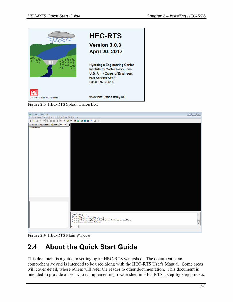
Figure 2.3 HEC-RTS Splash Dialog Box
Figure 2.4 HEC-RTS Main Window
About the Quick Start Guide This document is a guide to setting up an HEC-RTS watershed. The document is not comprehensive and is intended to be used along with the HEC-RTS User's Manual. Some areas will cover detail, where others will refer the reader to other documentation. This document is intended to provide a user who is implementing a watershed in HEC-RTS a step-by-step process.

Chapter 2 – Installing HEC-RTS HEC-RTS Quick Start Guide
2-4
Chapters 3 and 4 provide the user with an overview of the HEC-RTS framework. Chapter 5 introduces the user to creating an HEC-RTS study from scratch. Chapters 6 thru 9 are standalone chapters that lead a user thru creating an HEC-RTS study by importing individual models (Chapter 6); integrating models (Chapter 7); setting up the HEC-HMS model for forecast optimization (Chapter 8); and, incorporating Time Series Icons for both archived and real-time data (Chapters 9 and 10).
HEC-RTS Quick Start Guide Chapter 3 – HEC-RTS Interface
3-1
HEC-RTS Interface The graphical user interface (GUI) is the steering wheel of HEC-RTS. The GUI features graphical menus and tools organized by function, or modules. The four modules are:
• Setup for watershed configuration. • Acquisition for data acquisition, monitoring, validation, and editing. • Visualization for viewing data. • Modeling for setting up and executing analysis software for forecasting and viewing
results. This chapter provides an overview of the GUI and basic functions. Here are three navigation tips:
• For simplicity, the GUI "hides" commands that are not applicable to the module or element the user is working on. Thus, if an option appears to be missing, make sure that the correct module or element has been selected and that the option is applicable for that selection.
• Directory trees list elements configured in the watershed. When a user configures a new element, it will be added to the directory tree.
• Commands related to a selected element are typically accessible by right-clicking on the element.
Starting HEC-RTS
When starting HEC-RTS, double-click the HEC-RTS icon on a user's desktop if a shortcut has been placed there, or locate it in the folder where RTS was placed. The HEC-RTS splash dialog box will open (Figure 2.3). The splash dialog box appears for a few seconds, and then the main window of HEC-RTS will display (Figure 2.4). The user is now ready to start using HEC-RTS.
Opening an Existing Watershed In HEC-RTS, a watershed is a set of data, information, models, and images that represent lands and the channels, gages, and water control features within the watershed. A user may open an existing watershed from any of the modules. (If the user needs to create a new watershed, refer to Section 5.1. There are two methods available to open a watershed. First, if the user has opened the watershed before, from the HEC-RTS main window (Figure 2.4), from the File menu, point to Recent Watersheds, and click on the watershed name. The second way to open a watershed follows: 1. If watershed locations have not been set, from the HEC-RTS main window (Figure 2.4),
from the Tools menu, click Options. The Options dialog box will open (Figure 3.1).
Chapter 3 – HEC-RTS Interface HEC-RTS Quick Start Guide
3-2
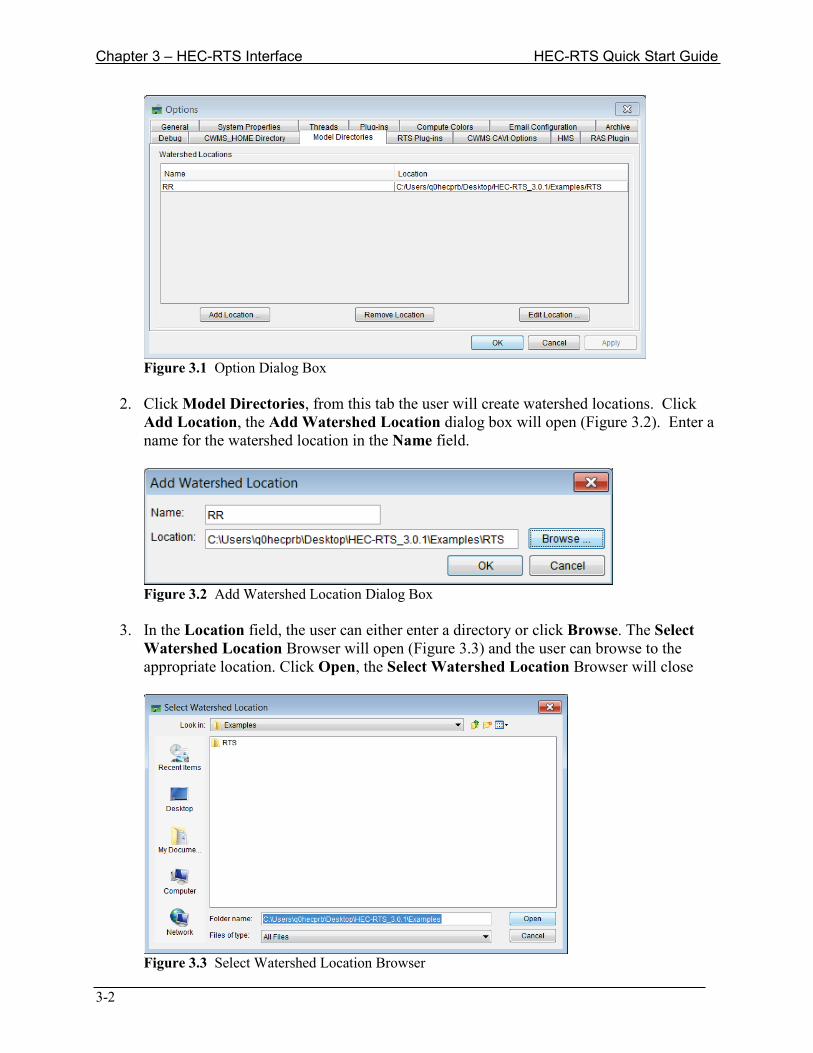
Figure 3.1 Option Dialog Box
2. Click Model Directories, from this tab the user will create watershed locations. Click
Add Location, the Add Watershed Location dialog box will open (Figure 3.2). Enter a name for the watershed location in the Name field.
Figure 3.2 Add Watershed Location Dialog Box
3. In the Location field, the user can either enter a directory or click Browse. The Select
Watershed Location Browser will open (Figure 3.3) and the user can browse to the appropriate location. Click Open, the Select Watershed Location Browser will close
Figure 3.3 Select Watershed Location Browser
HEC-RTS Quick Start Guide Chapter 3 – HEC-RTS Interface
3-3
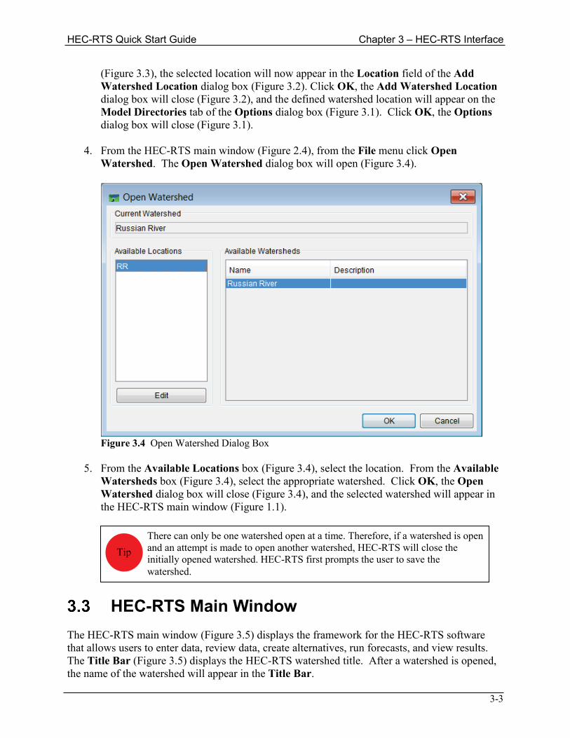
(Figure 3.3), the selected location will now appear in the Location field of the Add Watershed Location dialog box (Figure 3.2). Click OK, the Add Watershed Location dialog box will close (Figure 3.2), and the defined watershed location will appear on the Model Directories tab of the Options dialog box (Figure 3.1). Click OK, the Options dialog box will close (Figure 3.1).
4. From the HEC-RTS main window (Figure 2.4), from the File menu click Open
Watershed. The Open Watershed dialog box will open (Figure 3.4).
Figure 3.4 Open Watershed Dialog Box
5. From the Available Locations box (Figure 3.4), select the location. From the Available
Watersheds box (Figure 3.4), select the appropriate watershed. Click OK, the Open Watershed dialog box will close (Figure 3.4), and the selected watershed will appear in the HEC-RTS main window (Figure 1.1).
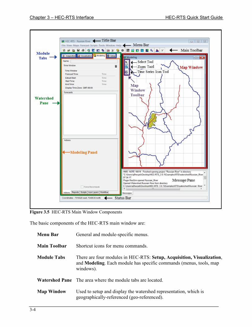
HEC-RTS Main Window The HEC-RTS main window (Figure 3.5) displays the framework for the HEC-RTS software that allows users to enter data, review data, create alternatives, run forecasts, and view results. The Title Bar (Figure 3.5) displays the HEC-RTS watershed title. After a watershed is opened, the name of the watershed will appear in the Title Bar.
There can only be one watershed open at a time. Therefore, if a watershed is open and an attempt is made to open another watershed, HEC-RTS will close the initially opened watershed. HEC-RTS first prompts the user to save the watershed.
Tip
Chapter 3 – HEC-RTS Interface HEC-RTS Quick Start Guide
3-4
Figure 3.5 HEC-RTS Main Window Components The basic components of the HEC-RTS main window are: Menu Bar General and module-specific menus. Main Toolbar Shortcut icons for menu commands. Module Tabs There are four modules in HEC-RTS: Setup, Acquisition, Visualization,
and Modeling. Each module has specific commands (menus, tools, map windows).
Watershed Pane The area where the module tabs are located. Map Window Used to setup and display the watershed representation, which is
geographically-referenced (geo-referenced).
HEC-RTS Quick Start Guide Chapter 3 – HEC-RTS Interface
3-5
Map Window Toolbar Tools used to setup and navigate within the map window. Messages Pane Displays a scrolling list of messages. System output log information
appears in this window from the time you start HEC-RTS until you exit. Messages related to incoming data are colored coded based on the quality of the data. Messages may also report a problem with a system component; problems with field equipment; a caution, warning, or flood event; or other critical situations.
Status Bar Displays map coordinates when the select tool is hovering over a location
in the map window. 3.3.1 Menu Bar The Menu Bar (Figure 3.5) of HEC-RTS provides the user with many commands to perform various functions. For more details check the HEC-RTS User's Manual. For this manual, an overview of each menu that is available in the HEC-RTS software is provided. File From this menu (appears in all modules), the user can create, open, close, upload, or
download a watershed; save data associated with the watershed; view watershed properties; print the map window; and, exit HEC-RTS. In addition, most recently opened watersheds are located at the bottom of the File menu. Available commands are: New Watershed, Open Watershed, Close Watershed, Upload/Download Watershed, Save Watershed, Save Watershed As, Watershed Properties, Print Map, Recent Watersheds, and Exit.
Edit This menu will appear in all modules and is module specific. Typically, the edit options will be relevant to data element(s) for a specific module.
View This menu is used to add or remove interface items (toolbar icons, the watershed pane, the messages bar, and the status bar); see what units, which time zone, and which coordinate system are being used for viewing; save, restore and manage layouts; choose whether or not to display the default computation point layer within the map window; select which modules tabs will be shown in the watershed pane; and view a list of watershed files.
Reports This menu is module specific and provides access to reports produced for the selected module.
Scripts This menu allows the user to execute existing scripts, create, test new scripts and run scripts. Available commands are: Script Editor, Schedule, Script Job Status, and Run.
Tools This menu allows the user to access data (HEC-DSSVue); utility software; set options for HEC-RTS; specify plug-in editor locations to use; view the "console.log" file; view log files of HEC-DSSVue and the other software applications; and, view memory usage. Available commands are: HEC-DSSVue, Applications, Options, Model Version Editor, Console Output, Logs, and Memory Monitor.
Chapter 3 – HEC-RTS Interface HEC-RTS Quick Start Guide
3-6
Window This menu allows the user to select how to view and select multiple windows, which modules the user wants to view. Available commands are: Duplicate Window, Detach Window, New Map Window, Map Window Properties, Sync Map Windows, Tile, Cascade, Next Window, and Previous Window.
Help Displays current version information about HEC-RTS.
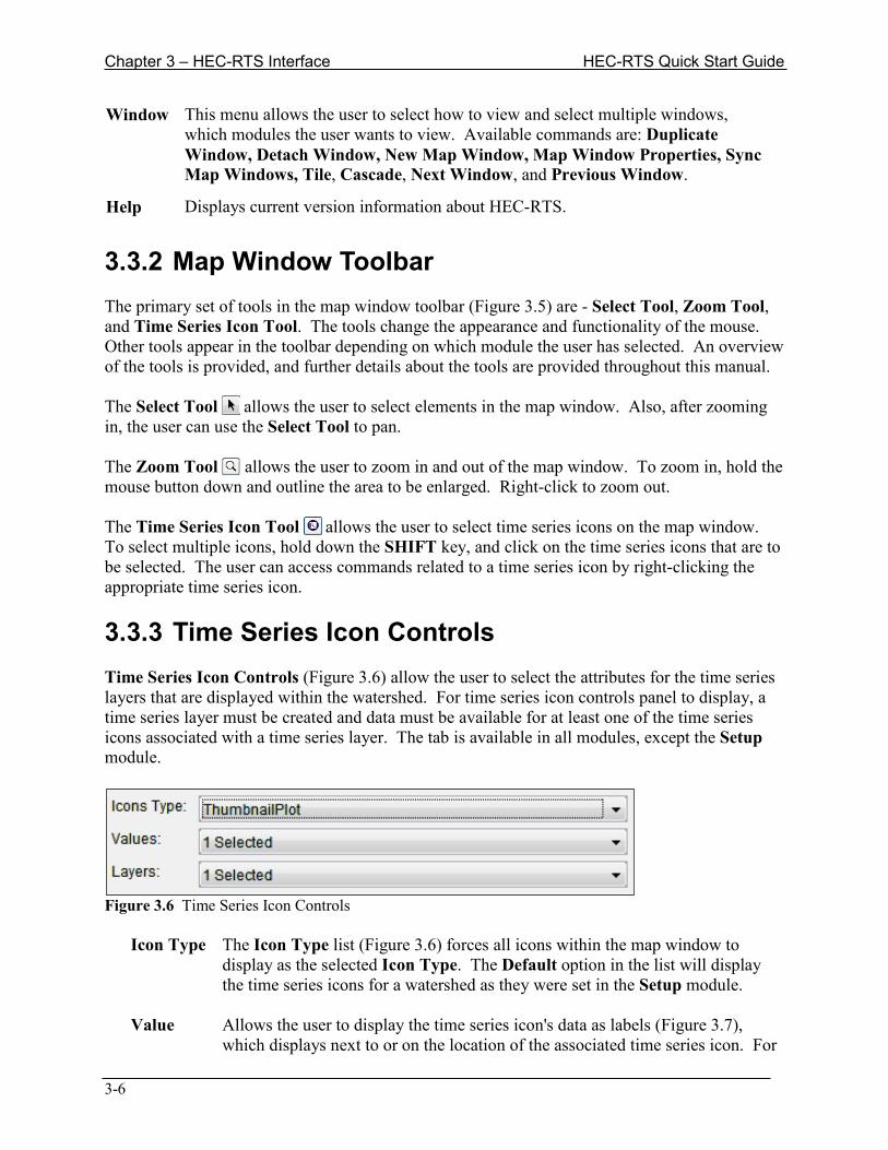
3.3.2 Map Window Toolbar The primary set of tools in the map window toolbar (Figure 3.5) are - Select Tool, Zoom Tool, and Time Series Icon Tool. The tools change the appearance and functionality of the mouse. Other tools appear in the toolbar depending on which module the user has selected. An overview of the tools is provided, and further details about the tools are provided throughout this manual. The Select Tool allows the user to select elements in the map window. Also, after zooming in, the user can use the Select Tool to pan. The Zoom Tool allows the user to zoom in and out of the map window. To zoom in, hold the mouse button down and outline the area to be enlarged. Right-click to zoom out. The Time Series Icon Tool allows the user to select time series icons on the map window. To select multiple icons, hold down the SHIFT key, and click on the time series icons that are to be selected. The user can access commands related to a time series icon by right-clicking the appropriate time series icon. 3.3.3 Time Series Icon Controls Time Series Icon Controls (Figure 3.6) allow the user to select the attributes for the time series layers that are displayed within the watershed. For time series icon controls panel to display, a time series layer must be created and data must be available for at least one of the time series icons associated with a time series layer. The tab is available in all modules, except the Setup module.
Figure 3.6 Time Series Icon Controls Icon Type The Icon Type list (Figure 3.6) forces all icons within the map window to
display as the selected Icon Type. The Default option in the list will display the time series icons for a watershed as they were set in the Setup module.
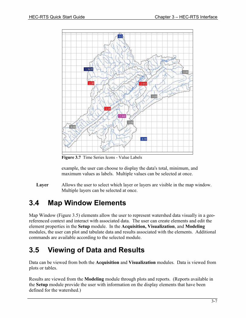
Value Allows the user to display the time series icon's data as labels (Figure 3.7),
which displays next to or on the location of the associated time series icon. For
HEC-RTS Quick Start Guide Chapter 3 – HEC-RTS Interface
3-7
Figure 3.7 Time Series Icons - Value Labels
example, the user can choose to display the data's total, minimum, and
maximum values as labels. Multiple values can be selected at once. Layer Allows the user to select which layer or layers are visible in the map window.
Multiple layers can be selected at once.
Map Window Elements Map Window (Figure 3.5) elements allow the user to represent watershed data visually in a geo-referenced context and interact with associated data. The user can create elements and edit the element properties in the Setup module. In the Acquisition, Visualization, and Modeling modules, the user can plot and tabulate data and results associated with the elements. Additional commands are available according to the selected module.
Viewing of Data and Results Data can be viewed from both the Acquisition and Visualization modules. Data is viewed from plots or tables. Results are viewed from the Modeling module through plots and reports. (Reports available in the Setup module provide the user with information on the display elements that have been defined for the watershed.)

Chapter 3 – HEC-RTS Interface HEC-RTS Quick Start Guide
3-8
HEC-RTS Quick Start Guide Chapter 4 – Reviewing Results
4-1
Reviewing Results
Viewing of Data and Results Data can be viewed from both the Acquisition and Visualization modules through plots or tables. Results are viewed from the Modeling module through plots and reports. (Reports available in the Setup module provide the user with information on the display elements that have been defined for the watershed.)
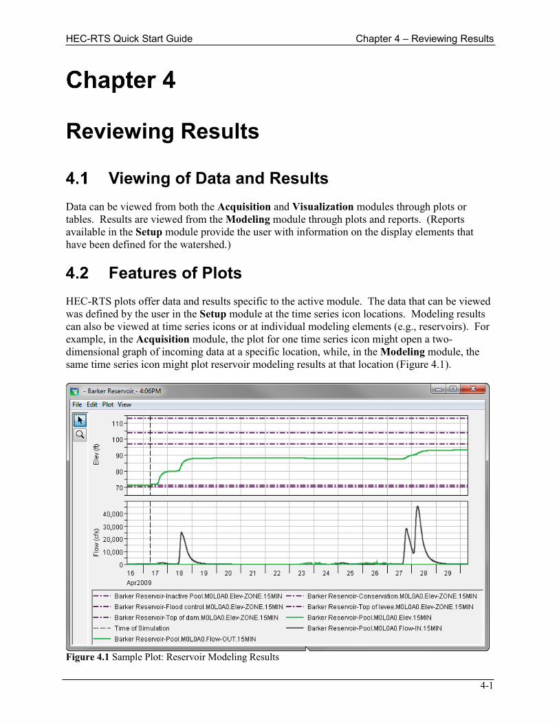
Features of Plots HEC-RTS plots offer data and results specific to the active module. The data that can be viewed was defined by the user in the Setup module at the time series icon locations. Modeling results can also be viewed at time series icons or at individual modeling elements (e.g., reservoirs). For example, in the Acquisition module, the plot for one time series icon might open a two-dimensional graph of incoming data at a specific location, while, in the Modeling module, the same time series icon might plot reservoir modeling results at that location (Figure 4.1).
Figure 4.1 Sample Plot: Reservoir Modeling Results

Chapter 4 – Reviewing Results HEC-RTS Quick Start Guide
4-2
The plot displays the location name in the title bar and has axis labels and a color-coded legend for the data contained in the plot. When a plot depicts results of a model alternative, as in Figure 4.1, a dashed vertical line represents the time of forecast. The Zoom Tool from the plot window operates the same as described in Section 3.3.2. The user can customize the appearance of plots through the use of several editors. To access these editors, use the Select Tool and right-click on different elements of the plot (e.g., lines, axis). The user can also access these editors through the Edit and View menus in the Plot dialog box (Figure 4.1). The following provides an overview of the different editors (see Appendix I of the HEC-RTS User’s Manual for more details on customizing plots):
Curve Properties Right-clicking on a plot curve or point allows the user to open a curve properties editor where curve colors, styles, and weights as well as labels and quality symbols can be edited.
Viewport Properties Right-clicking on the viewport of a plot allows the user to open an editor where the border, background, and gridlines of the plot can be customized.
Title Properties Right-clicking on a plot axis allows the user to open a title properties editor where the title of a plot can be customized.
Axis Properties Right-clicking on a plot axis allows the user to open an axis properties editor where the axis scale and tic marks can be customized.
Legend Properties Right-clicking on the legend of a plot allows the user to open an editor where the user can add a title and add icons and text to the left and right blocks of a plot.
Label Properties Right-clicking on an axis label or plot legend allows the user to open a label properties editor where the user can add or change the background color of labels or add a border to the labels.
Spacer Properties If multiple plots are available in the plot window, the user can right-click on the space between the plots to access the Space Properties Editor. From the Space Properties Editor adjustments can be made to the space between plots.
Polygon Properties Right-clicking on a polygon allows the user to open a polygon properties editor where borders and backgrounds can be customized.
Features of Tables
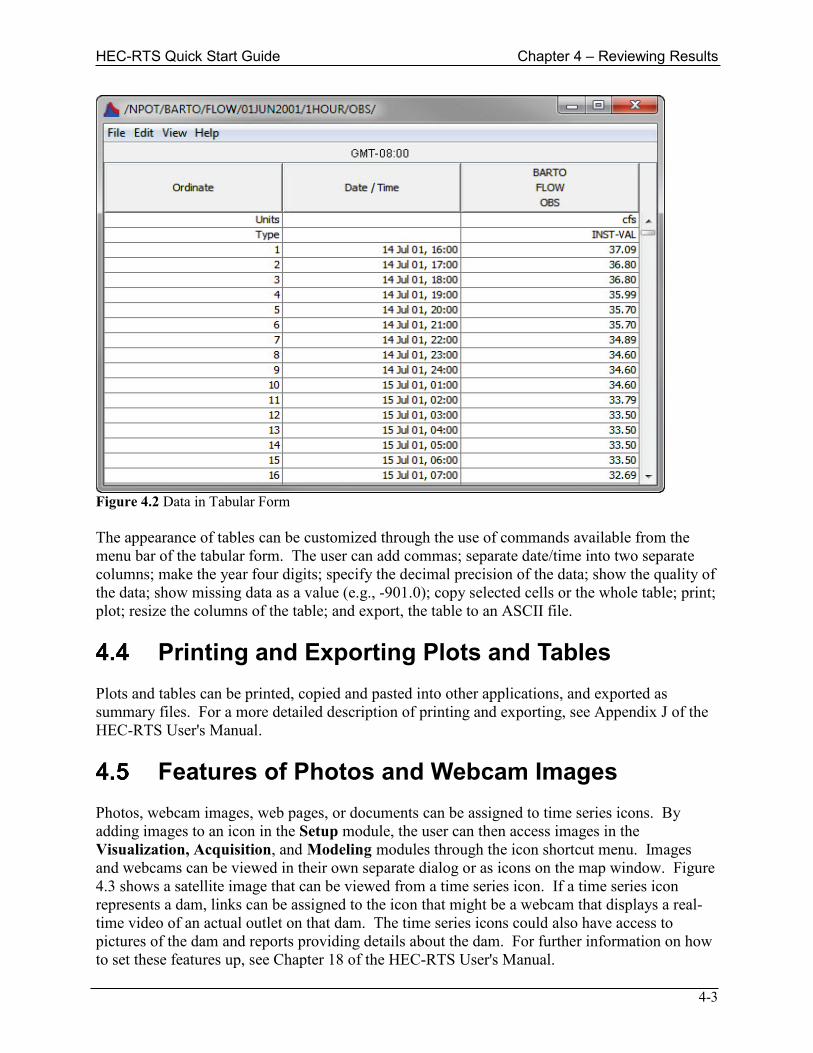
The same data and information viewed from a plot can also be viewed in tabular form (Figure 4.2). As with plots, the type of data and results displayed depends on the properties the user defined for each time series icon.
HEC-RTS Quick Start Guide Chapter 4 – Reviewing Results
4-3
Figure 4.2 Data in Tabular Form The appearance of tables can be customized through the use of commands available from the menu bar of the tabular form. The user can add commas; separate date/time into two separate columns; make the year four digits; specify the decimal precision of the data; show the quality of the data; show missing data as a value (e.g., -901.0); copy selected cells or the whole table; print; plot; resize the columns of the table; and export, the table to an ASCII file.
Printing and Exporting Plots and Tables Plots and tables can be printed, copied and pasted into other applications, and exported as summary files. For a more detailed description of printing and exporting, see Appendix J of the HEC-RTS User's Manual.
Features of Photos and Webcam Images Photos, webcam images, web pages, or documents can be assigned to time series icons. By adding images to an icon in the Setup module, the user can then access images in the Visualization, Acquisition, and Modeling modules through the icon shortcut menu. Images and webcams can be viewed in their own separate dialog or as icons on the map window. Figure 4.3 shows a satellite image that can be viewed from a time series icon. If a time series icon represents a dam, links can be assigned to the icon that might be a webcam that displays a real-time video of an actual outlet on that dam. The time series icons could also have access to pictures of the dam and reports providing details about the dam. For further information on how to set these features up, see Chapter 18 of the HEC-RTS User's Manual.

Chapter 4 – Reviewing Results HEC-RTS Quick Start Guide
4-4
Figure 4.3 Viewing an Image from a Time Series Icon
Running Scripts from Icons Scripts can be assigned to individual time series icons. The scripts can be used to update the data at given intervals, compute other information from the data, or complete other tasks. Scripts are assigned to the icons in the Setup module, through the Time Series Icon Editor. Scripts can also be created in the provided Script Editor. For more detailed information on assigning and using scripts, see Appendix H of the HEC-RTS User's Manual.
HEC-RTS Quick Start Guide Chapter 5 – Create a new HEC-RTS Watershed
5-1
Create a New HEC-RTS Watershed
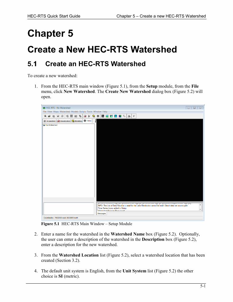
Create an HEC-RTS Watershed To create a new watershed: 1. From the HEC-RTS main window (Figure 5.1), from the Setup module, from the File
menu, click New Watershed. The Create New Watershed dialog box (Figure 5.2) will open.
Figure 5.1 HEC-RTS Main Window – Setup Module
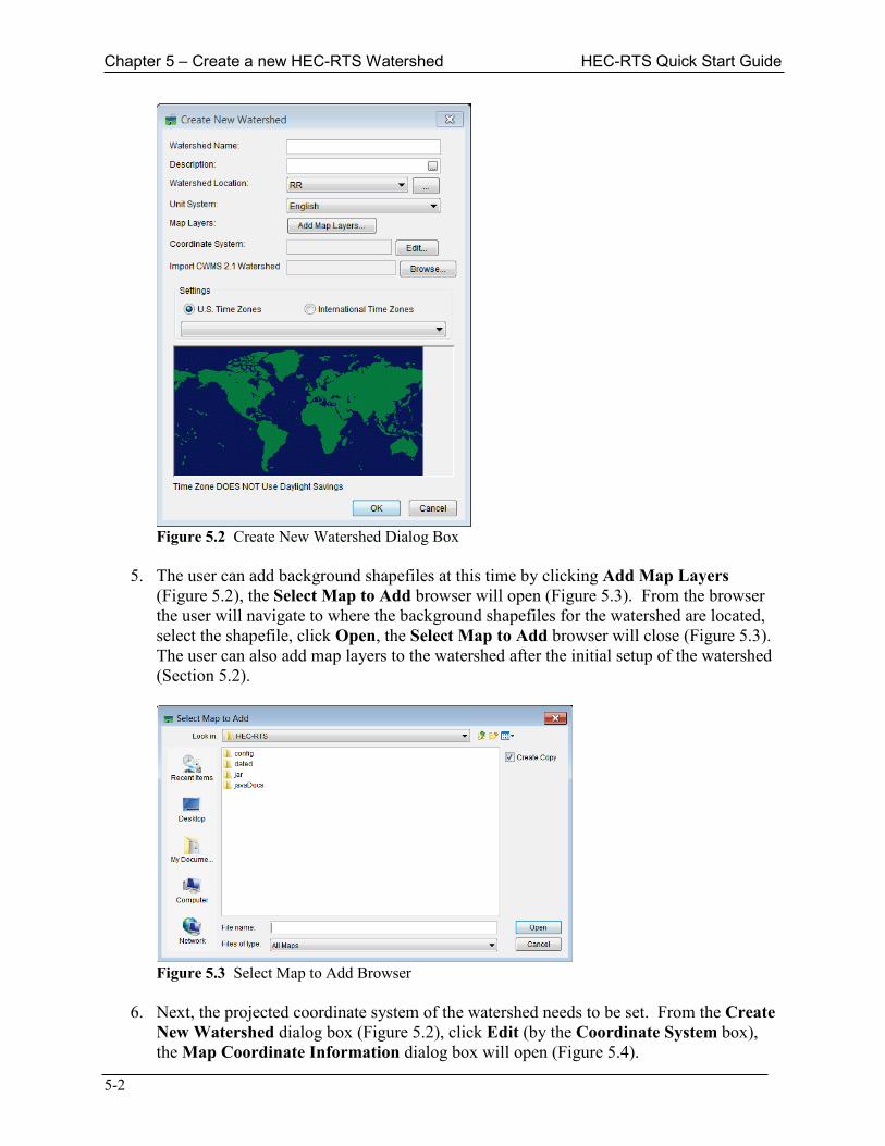
2. Enter a name for the watershed in the Watershed Name box (Figure 5.2). Optionally,
the user can enter a description of the watershed in the Description box (Figure 5.2), enter a description for the new watershed.
3. From the Watershed Location list (Figure 5.2), select a watershed location that has been
created (Section 3.2). 4. The default unit system is English, from the Unit System list (Figure 5.2) the other
choice is SI (metric).
Chapter 5 – Create a new HEC-RTS Watershed HEC-RTS Quick Start Guide
5-2
Figure 5.2 Create New Watershed Dialog Box
5. The user can add background shapefiles at this time by clicking Add Map Layers
(Figure 5.2), the Select Map to Add browser will open (Figure 5.3). From the browser the user will navigate to where the background shapefiles for the watershed are located, select the shapefile, click Open, the Select Map to Add browser will close (Figure 5.3). The user can also add map layers to the watershed after the initial setup of the watershed (Section 5.2).
Figure 5.3 Select Map to Add Browser
6. Next, the projected coordinate system of the watershed needs to be set. From the Create
New Watershed dialog box (Figure 5.2), click Edit (by the Coordinate System box), the Map Coordinate Information dialog box will open (Figure 5.4).
HEC-RTS Quick Start Guide Chapter 5 – Create a new HEC-RTS Watershed
5-3
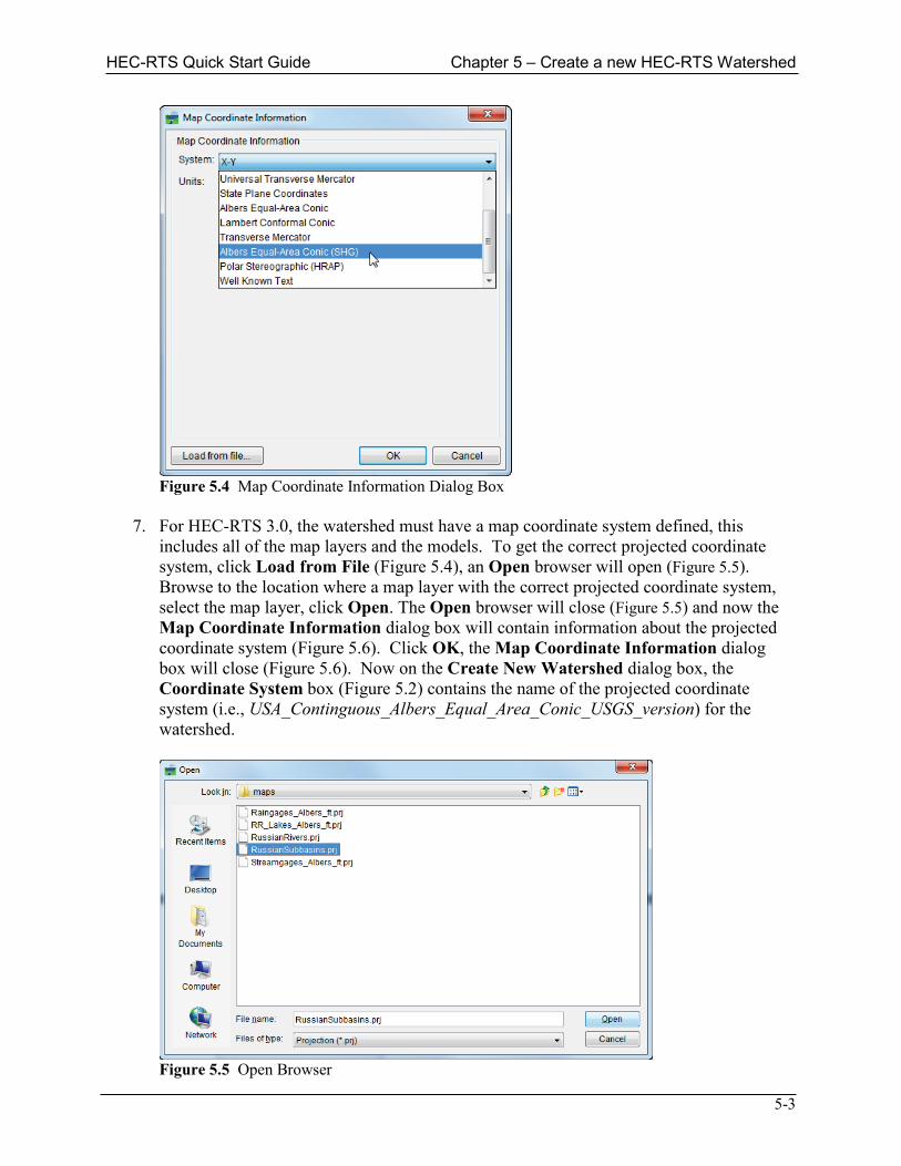
Figure 5.4 Map Coordinate Information Dialog Box
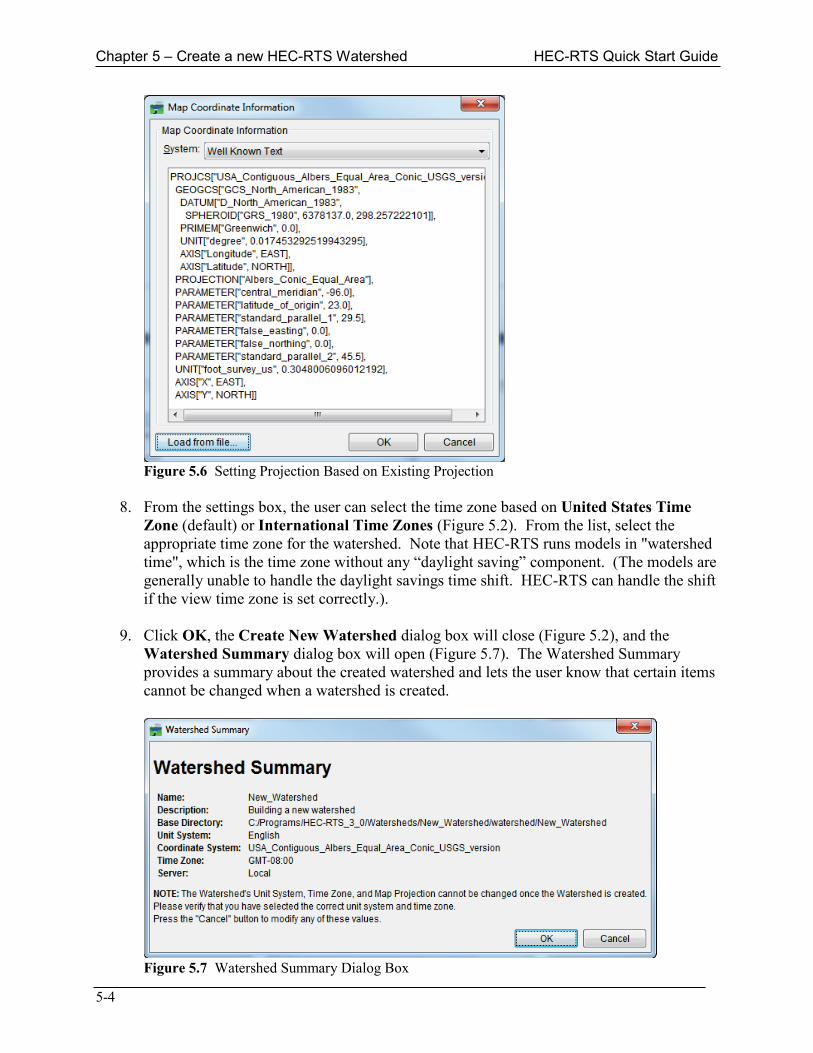
7. For HEC-RTS 3.0, the watershed must have a map coordinate system defined, this
includes all of the map layers and the models. To get the correct projected coordinate system, click Load from File (Figure 5.4), an Open browser will open (Figure 5.5). Browse to the location where a map layer with the correct projected coordinate system, select the map layer, click Open. The Open browser will close (Figure 5.5) and now the Map Coordinate Information dialog box will contain information about the projected coordinate system (Figure 5.6). Click OK, the Map Coordinate Information dialog box will close (Figure 5.6). Now on the Create New Watershed dialog box, the Coordinate System box (Figure 5.2) contains the name of the projected coordinate system (i.e., USA_Continguous_Albers_Equal_Area_Conic_USGS_version) for the watershed.
Figure 5.5 Open Browser
Chapter 5 – Create a new HEC-RTS Watershed HEC-RTS Quick Start Guide
5-4
Figure 5.6 Setting Projection Based on Existing Projection
8. From the settings box, the user can select the time zone based on United States Time
Zone (default) or International Time Zones (Figure 5.2). From the list, select the appropriate time zone for the watershed. Note that HEC-RTS runs models in "watershed time", which is the time zone without any “daylight saving” component. (The models are generally unable to handle the daylight savings time shift. HEC-RTS can handle the shift if the view time zone is set correctly.).
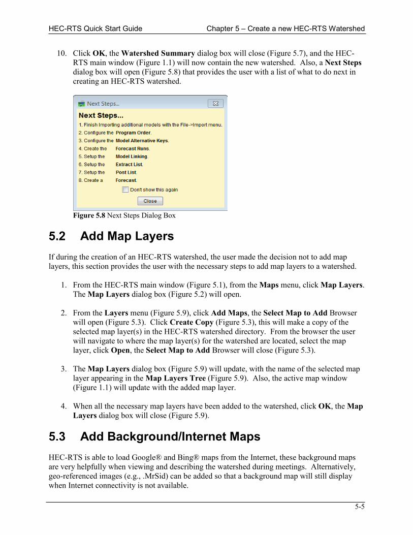
9. Click OK, the Create New Watershed dialog box will close (Figure 5.2), and the
Watershed Summary dialog box will open (Figure 5.7). The Watershed Summary provides a summary about the created watershed and lets the user know that certain items cannot be changed when a watershed is created.
Figure 5.7 Watershed Summary Dialog Box
HEC-RTS Quick Start Guide Chapter 5 – Create a new HEC-RTS Watershed
5-5
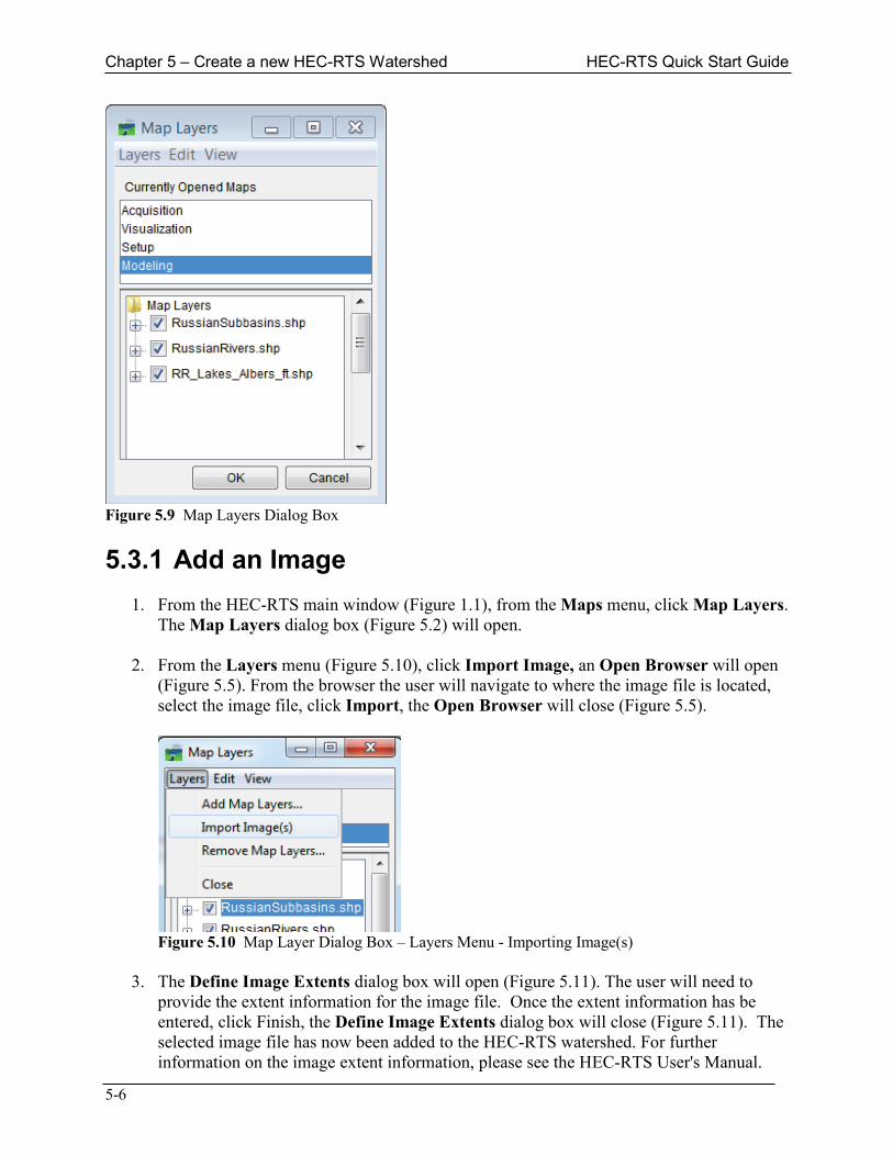
10. Click OK, the Watershed Summary dialog box will close (Figure 5.7), and the HEC-RTS main window (Figure 1.1) will now contain the new watershed. Also, a Next Steps dialog box will open (Figure 5.8) that provides the user with a list of what to do next in creating an HEC-RTS watershed.
Figure 5.8 Next Steps Dialog Box
Add Map Layers
If during the creation of an HEC-RTS watershed, the user made the decision not to add map layers, this section provides the user with the necessary steps to add map layers to a watershed. 1. From the HEC-RTS main window (Figure 5.1), from the Maps menu, click Map Layers.
The Map Layers dialog box (Figure 5.2) will open. 2. From the Layers menu (Figure 5.9), click Add Maps, the Select Map to Add Browser
will open (Figure 5.3). Click Create Copy (Figure 5.3), this will make a copy of the selected map layer(s) in the HEC-RTS watershed directory. From the browser the user will navigate to where the map layer(s) for the watershed are located, select the map layer, click Open, the Select Map to Add Browser will close (Figure 5.3).
3. The Map Layers dialog box (Figure 5.9) will update, with the name of the selected map
layer appearing in the Map Layers Tree (Figure 5.9). Also, the active map window (Figure 1.1) will update with the added map layer.
4. When all the necessary map layers have been added to the watershed, click OK, the Map
Layers dialog box will close (Figure 5.9).
Add Background/Internet Maps HEC-RTS is able to load Google® and Bing® maps from the Internet, these background maps are very helpfully when viewing and describing the watershed during meetings. Alternatively, geo-referenced images (e.g., .MrSid) can be added so that a background map will still display when Internet connectivity is not available.
Chapter 5 – Create a new HEC-RTS Watershed HEC-RTS Quick Start Guide
5-6
Figure 5.9 Map Layers Dialog Box 5.3.1 Add an Image 1. From the HEC-RTS main window (Figure 1.1), from the Maps menu, click Map Layers.
The Map Layers dialog box (Figure 5.2) will open. 2. From the Layers menu (Figure 5.10), click Import Image, an Open Browser will open
(Figure 5.5). From the browser the user will navigate to where the image file is located, select the image file, click Import, the Open Browser will close (Figure 5.5).
Figure 5.10 Map Layer Dialog Box – Layers Menu - Importing Image(s)
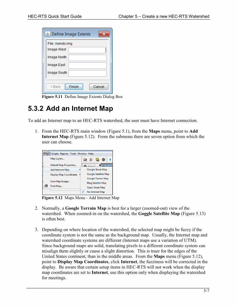
3. The Define Image Extents dialog box will open (Figure 5.11). The user will need to
provide the extent information for the image file. Once the extent information has be entered, click Finish, the Define Image Extents dialog box will close (Figure 5.11). The selected image file has now been added to the HEC-RTS watershed. For further information on the image extent information, please see the HEC-RTS User's Manual.
HEC-RTS Quick Start Guide Chapter 5 – Create a new HEC-RTS Watershed
5-7
Figure 5.11 Define Image Extents Dialog Box
5.3.2 Add an Internet Map To add an Internet map to an HEC-RTS watershed, the user must have Internet connection. 1. From the HEC-RTS main window (Figure 5.1), from the Maps menu, point to Add
Internet Map (Figure 5.12). From the submenu there are seven option from which the user can choose.
Figure 5.12 Maps Menu - Add Internet Map
2. Normally, a Google Terrain Map is best for a larger (zoomed-out) view of the
watershed. When zoomed-in on the watershed, the Goggle Satellite Map (Figure 5.13) is often best.
3. Depending on where location of the watershed, the selected map might be fuzzy if the
coordinate system is not the same as the background map. Usually, the Internet map and watershed coordinate systems are different (Internet maps use a variation of UTM). Since background maps are solid, translating pixels to a different coordinate system can misalign them slightly or cause a slight distortion. This is truer for the edges of the United States continent, than in the middle areas. From the Maps menu (Figure 5.12), point to Display Map Coordinates, click Internet, the fuzziness will be corrected in the display. Be aware that certain setup items in HEC-RTS will not work when the display map coordinates are set to Internet, use this option only when displaying the watershed for meetings.
Chapter 5 – Create a new HEC-RTS Watershed HEC-RTS Quick Start Guide
5-8
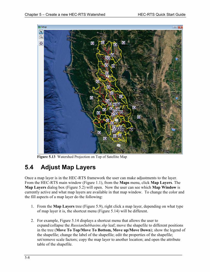
Figure 5.13 Watershed Projection on Top of Satellite Map
Adjust Map Layers
Once a map layer is in the HEC-RTS framework the user can make adjustments to the layer. From the HEC-RTS main window (Figure 1.1), from the Maps menu, click Map Layers. The Map Layers dialog box (Figure 5.2) will open. Now the user can see which Map Window is currently active and what map layers are available in that map window. To change the color and the fill aspects of a map layer do the following: 1. From the Map Layers tree (Figure 5.9), right click a map layer, depending on what type
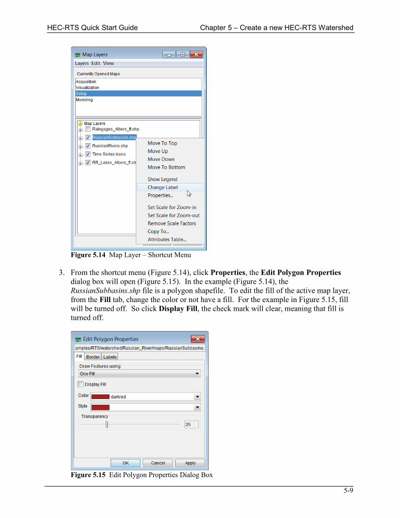
of map layer it is, the shortcut menu (Figure 5.14) will be different. 2. For example, Figure 5.14 displays a shortcut menu that allows the user to
expand/collapse the RussianSubbasins.shp leaf; move the shapefile to different positions in the tree (Move To Top/Move To Bottom, Move up/Move Down); show the legend of the shapefile; change the label of the shapefile; edit the properties of the shapefile; set/remove scale factors; copy the map layer to another location; and open the attribute table of the shapefile.
HEC-RTS Quick Start Guide Chapter 5 – Create a new HEC-RTS Watershed
5-9
Figure 5.14 Map Layer – Shortcut Menu
3. From the shortcut menu (Figure 5.14), click Properties, the Edit Polygon Properties
dialog box will open (Figure 5.15). In the example (Figure 5.14), the RussianSubbasins.shp file is a polygon shapefile. To edit the fill of the active map layer, from the Fill tab, change the color or not have a fill. For the example in Figure 5.15, fill will be turned off. So click Display Fill, the check mark will clear, meaning that fill is turned off.
Figure 5.15 Edit Polygon Properties Dialog Box
Chapter 5 – Create a new HEC-RTS Watershed HEC-RTS Quick Start Guide
5-10
3. To turn off a map layer - click in the checkbox by Raingages_Albers_ft.shp, the rain gages no longer appear on the map window.
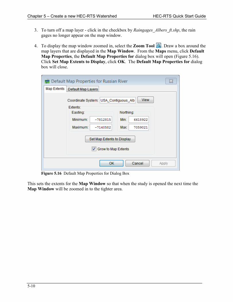
4. To display the map window zoomed in, select the Zoom Tool . Draw a box around the
map layers that are displayed in the Map Window. From the Maps menu, click Default Map Properties, the Default Map Properties for dialog box will open (Figure 5.16). Click Set Map Extents to Display, click OK. The Default Map Properties for dialog box will close.
Figure 5.16 Default Map Properties for Dialog Box
This sets the extents for the Map Window so that when the study is opened the next time the Map Window will be zoomed in to the tighter area.
HEC-RTS Quick Start Guide Chapter 6 – Importing Models
6-1
Importing Models Before importing any models:
• Be sure that models run without errors. If the model does not run outside of HEC-RTS, the model will not run inside of HEC-RTS. Fix any problems before importing.
• Where possible, use relative paths to files, not absolute paths.
• The directories where models are located are "clean". Backup original directories and remove all log, output and temporary files. Also, remove DSS files containing historical data used for calibration. Keep DSS files that contain model parameters, such as storage-elevation-area curves. Have a trim, pristine directory with only those files needed for real-time execution.
• Keep blank spaces and dashes out of names and files; for example, HEC-HMS will change dashes "-" to underscores "_" without HEC-RTS knowing it. Do not use unnecessary non-alpha characters.
• Many errors have arisen due to either messy directories or not checking that models run correctly on the PC environment. Errors are more difficult to track down through HEC-RTS than directly from the models themselves.
Program Order
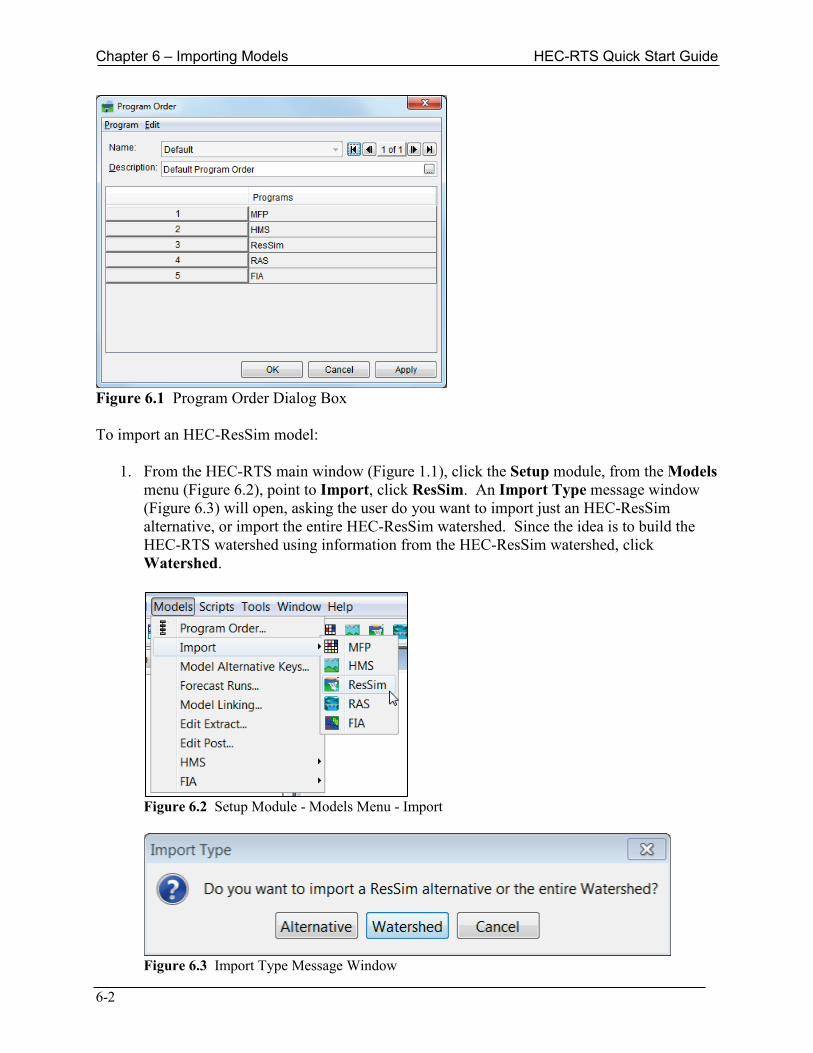
HEC-RTS can run with zero to four models. The user should setup a program order to only include those models that will run. For example, if the interest is in forecasting local flow and stage, and real-time inundation maps, then the Program Order might only include HEC-HMS and HEC-RAS. From the HEC-RTS main window (Figure 1.1), click Setup module, from the Models menu, click Program Order. The Program Order dialog box will open (Figure 6.1), displaying the default program order. The program order identifies which models will be run and the order in which those models will be run. A user can create a new program order and add or remove programs, for this manual, the default program order will be used. Refer to Chapter 16 of the HEC-RTS User's Manual for further details.
Import an HEC-Res-Sim Model Since the HEC-ResSim model contains the Stream Alignment and other elements that describe the watershed, it is recommended that the user import the HEC-ResSim model first for an HEC-RTS watershed.
Chapter 6 – Importing Models HEC-RTS Quick Start Guide
6-2
Figure 6.1 Program Order Dialog Box To import an HEC-ResSim model: 1. From the HEC-RTS main window (Figure 1.1), click the Setup module, from the Models
menu (Figure 6.2), point to Import, click ResSim. An Import Type message window (Figure 6.3) will open, asking the user do you want to import just an HEC-ResSim alternative, or import the entire HEC-ResSim watershed. Since the idea is to build the HEC-RTS watershed using information from the HEC-ResSim watershed, click Watershed.
Figure 6.2 Setup Module - Models Menu - Import
Figure 6.3 Import Type Message Window

HEC-RTS Quick Start Guide Chapter 6 – Importing Models
6-3
2. A Select Watershed File to Import From Browser will open (Figure 6.4). From the browser the user will navigate to where the HEC-ResSim model is located, select a *.wksp file, click Open, the Select Watershed File to Import From Browser will close (Figure 6.4).
Figure 6.4 Select Watershed File to Import From Browser
3. A ResSim import progress dialog box will open, once the import is finished an Import
Finished message window (Figure 6.5) will open. Click OK, the Import Finished message window (Figure 6.5) will close, the stream alignment will display in the map window, and from the watershed tree (Figure 6.6), from the Models folder, expand ResSim, and the list of HEC-ResSim alternatives is displayed.
Figure 6.5 Import Finished Message Window
Import an HEC-HMS Model
Now let's import the HEC-HMS model into the HEC-RTS watershed. Depending on what version of HEC-HMS the model was built with, during the import process HEC-HMS may automatically update the HEC-HMS model to the current version. The HEC-HMS model will no longer work with the version the model was created in, so a full back up of the HEC-HMS model is recommended.

Chapter 6 – Importing Models HEC-RTS Quick Start Guide
6-4
Figure 6.6 HEC-RTS Main Window – Watershed Tree - ResSim Alternatives To import an HEC-HMS model: 1. From the HEC-RTS main window (Figure 1.1), click the Setup module, from the Models
menu (Figure 6.2), point to Import, click HMS. An HEC-HMS Select Project File Browser will open (Figure 6.7). From the browser the user will navigate to where the HEC-HMS model is located, select a *.hms file, click Select, the Select Project File Browser will close (Figure 6.7).
Figure 6.7 HEC-HMS Select Project File Browser
2. The HEC-HMS import process will begin, when the import of the HEC-HMS model is
complete, the user is returned to the HEC-RTS main window (Figure 1.1). From the Watershed Tree (Figure 6.6), from the Models folder, expand HMS, and the list of HEC-HMS runs is displayed.

HEC-RTS Quick Start Guide Chapter 6 – Importing Models
6-5
Create MFP Alternatives
Once the HEC-HMS model has been imported, the user can now create an MFP (Meteorological Forecast Processer) alternative. MFP is a rather simple process that takes observed precipitation grids and combines it with forecasted precipitation grids to make a continuous set of grids for HEC-HMS to run with. The first alternative that a user might create would be "no future precipitation", with zero precipitation after the "time of forecast". To create an MFP alternative: 1. From the HEC-RTS main window (Figure 1.1), click the Setup module, from the
Watershed Tree menu (Figure 6.8), right-click MFP (Figure 6.8). From the shortcut menu (Figure 6.8), click New, the Create New MFP Alterative dialog box will open (Figure 6.9).
Figure 6.8 Watershed Tree – MFP Shortcut Menu
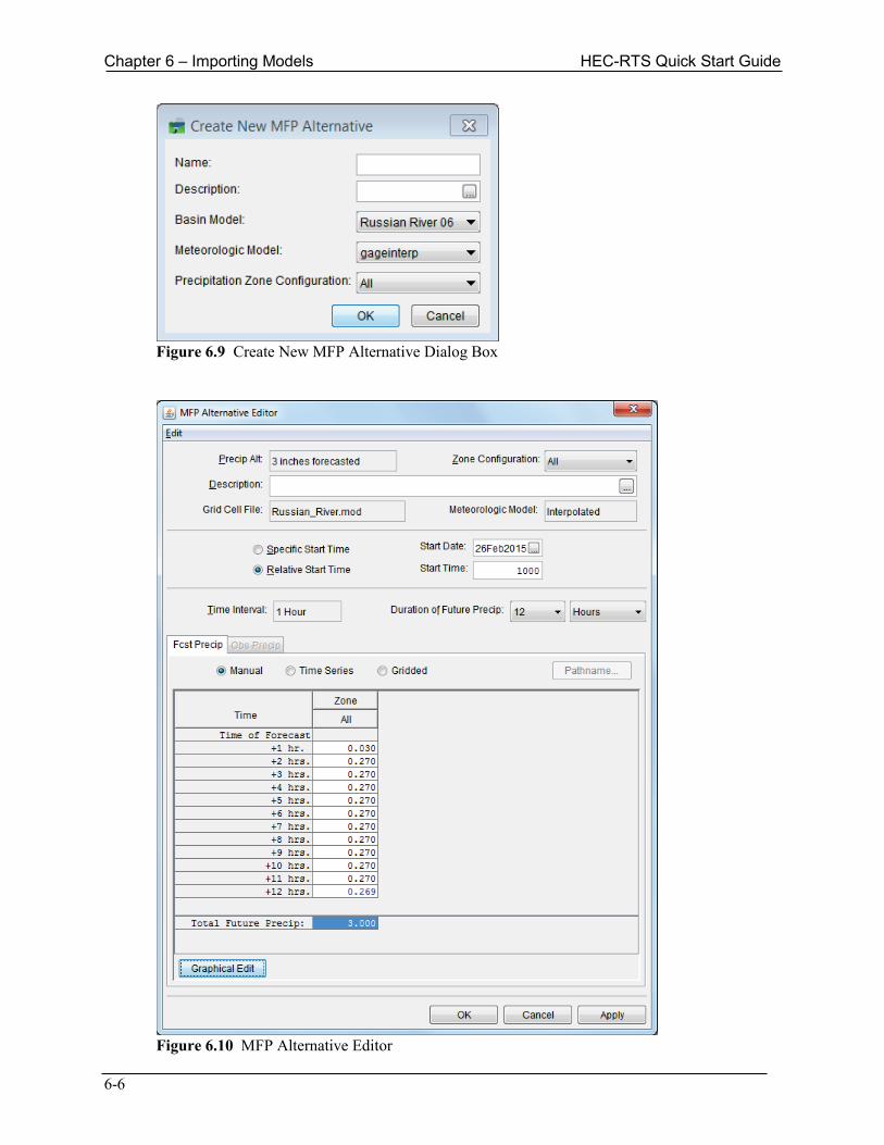
2. Enter a name for the MFP alternative in the Name box (Figure 6.9). The user can enter
an optional description about the MFP alternative in the Description box (Figure 6.9). From the Basin Model list (Figure 6.9), select the appropriate HEC-HMS basin model. Next, the user needs to select the appropriate HEC-HMS meteorologic model from the Meteorologic Model list (Figure 6.9). The last item to configure is the number of precipitation zones, Precipitation Zone Configuration list (Figure 6.9).
3. Click OK, the Create New MFP Alterative dialog box will close (Figure 6.9). From the
Watershed Tree (Figure 6.6), from the Models folder, expand MFP, and the name of the created MFP alternative is listed. From the Watershed Tree, right-click on an MFP alternative, from the shortcut menu click Edit Alternative, the MFP Alternative Editor will open (Figure 6.10). Further information (future precipitation, temporal distribution) for the MFP alternative needs to be input (refer to the HEC-RTS User's Manual for further information).
Chapter 6 – Importing Models HEC-RTS Quick Start Guide
6-6
Figure 6.9 Create New MFP Alternative Dialog Box
Figure 6.10 MFP Alternative Editor

HEC-RTS Quick Start Guide Chapter 6 – Importing Models
6-7
Import an HEC-RAS Model Now let's import the HEC-RAS model into the HEC-RTS watershed: 1. From the HEC-RTS main window (Figure 1.1), click the Setup module, from the Models
menu (Figure 6.2), point to Import, click RAS. A Select RAS project to import from Browser will open (Figure 6.11). From the browser the user will navigate to where the HEC-RAS model is located, select a *.prj file, click Open, the Select RAS project to import from Browser will close (Figure 6.11).
Figure 6.11 Select RAS project to import from Browser
2. The HEC-RAS import process will begin, when the import of the HEC-RAS model is
complete, the user is returned to the HEC-RTS main window (Figure 1.1). From the Watershed Tree (Figure 6.6), from the Models folder, expand RAS, and the list of HEC-RAS plans is displayed.
Import an HEC-FIA Model
For the HEC-FIA import, the HEC-FIA model needs to have been built with HEC-FIA Verison 3.0 or later; the import process will not import any EC-FIA models that were built with earlier versions of HEC-FIA. 1. From the HEC-RTS main window (Figure 1.1), click the Setup module, from the
Models menu (Figure 6.2), point to Import, click FIA. An Import Alternatives dialog box will open (Figure 6.12).
2. Click Select/Add Project (Figure 6.12), an Open Browser will open (Figure 5.5). From
the browser the user will navigate to where the HEC-FIA model is located, select a *.prj file, click Open, the Open Browser will close (Figure 5.5).

Chapter 6 – Importing Models HEC-RTS Quick Start Guide
6-8
Figure 6.12 Import Alternatives Dialog Box
3. The table in the Please Select Your Alternative For Each Project box (Figure 6.12)
will list the selected HEC-FIA model. From the Alterative List (Figure 6.12), select the HEC-FIA alternative to be used in the HEC-RTS watershed.
4. Click Import Alternatives (Figure 6.12), the import will start, and in the Progress
column of the table (Figure 6.12) a green progress bar will display letting the user know how the import is progressing. An Information message window (Figure 6.13) will display when the HEC-FIA model import is finished, click OK. The Information message window (Figure 6.13) will close.
Figure 6.13 Information Message Window
5. From the Import Alternatives dialog box (Figure 6.12) click Close, the Import
Alternatives dialog box will close (Figure 6.12). The user is returned to the HEC-RTS main window (Figure 1.1). From the Watershed Tree (Figure 6.6), from the Models folder, expand FIA, and the list of HEC-FIA alternatives is displayed.
All the models have been imported, the next step is to associate alternatives keys (used in the F-part of the DSS pathname) with each model's alternatives, and then link the model alternatives together – model integration.
HEC-RTS Quick Start Guide Chapter 7 – Model Integration
7-1
Model Integration Data is exchanged between models in an HEC-RTS forecast using a DSS file and with pathnames that contain an F-part that identify the model and scenario (alternative). Each individual model or model input/output is called an Alternative. An alternative may be different reservoir operations, or a different forecast for precipitation, or different loss or routing parameters. For example, typically in an HEC-RTS study, there might be at least three (future) precipitation alternatives - No Future Precipitation, QPF, User Specified. Each model alternative is assigned an alpha-numeric character, or "key", that identifies the alternative. Different models may use the same character (e.g., B for base HMS and B for a ResSim alternative.) The model alternative keys are concatenated together to form a "Run Key", which is used in the F-part of a DSS pathname to identify the dataset. For example, for a QPF alternative for MFP, which combines observed precipitation and future precipitation, the MFP alternative would be assigned the letter "Q". The HEC-HMS model needs the precipitation from the MFP alternative to generate flows, both observed and forecasted. So, HEC-HMS would look for pathnames with an F-part of "Q". The HEC-HMS model was calibrated for wet conditions, so the HEC-HMS alternative might be assigned the letter "W". The HEC-ResSim needs the HEC-HMS flows, so HEC-ResSim would be looking for pathnames with an F-part of "QW". The HEC-ResSim model is a standard operation model which means the assignment might be the key "S". HEC-RAS model needs the flows out of the reservoir, so HEC-RAS would be looking for pathnames with an F-part of "QWS". HEC-RAS then compute stages and writes those stages out to pathnames with an F-part of "QWSB" (the HEC-RAS model having a key of "B"). In turn, the HEC-FIA model would need the stages from the HEC-RAS model and would be looking for pathnames with an F-part of "QWSB". Reports, output, log files, etc. all use this convention to identify the complete dataset that they represent. In short, if a "%" represents a model, then log files and the F-parts of the DSS pathnames used will be:
• % - output from MFP • %% - output from HEC-HMS • %%% - output from HEC-ResSim • %%%% - output from HEC-RAS • %%%%% - output from HEC-FIA
The user can use these percent signs in the model interface module to identify datasets, especially in time series icons to identify what DSS datasets to use. Currently, a "trial" number (0) is internally appended to each ID key and will appear in the F-part. Trials in HEC-RTS will not be addressed at this time.
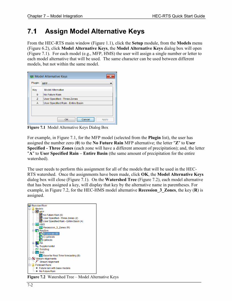
Chapter 7 – Model Integration HEC-RTS Quick Start Guide
7-2
Assign Model Alternative Keys From the HEC-RTS main window (Figure 1.1), click the Setup module, from the Models menu (Figure 6.2), click Model Alternative Keys, the Model Alternative Keys dialog box will open (Figure 7.1). For each model (e.g., MFP, HMS) the user will assign a single number or letter to each model alternative that will be used. The same character can be used between different models, but not within the same model.
Figure 7.1 Model Alternative Keys Dialog Box For example, in Figure 7.1, for the MFP model (selected from the Plugin list), the user has assigned the number zero (0) to the No Future Rain MFP alternative; the letter "Z" to User Specified - Three Zones (each zone will have a different amount of precipitation); and, the letter "A" to User Specified Rain – Entire Basin (the same amount of precipitation for the entire watershed). The user needs to perform this assignment for all of the models that will be used in the HEC-RTS watershed. Once the assignments have been made, click OK, the Model Alternative Keys dialog box will close (Figure 7.1). On the Watershed Tree (Figure 7.2), each model alternative that has been assigned a key, will display that key by the alternative name in parentheses. For example, in Figure 7.2, for the HEC-HMS model alternative Recession_3_Zones, the key (R) is assigned.
Figure 7.2 Watershed Tree – Model Alternative Keys
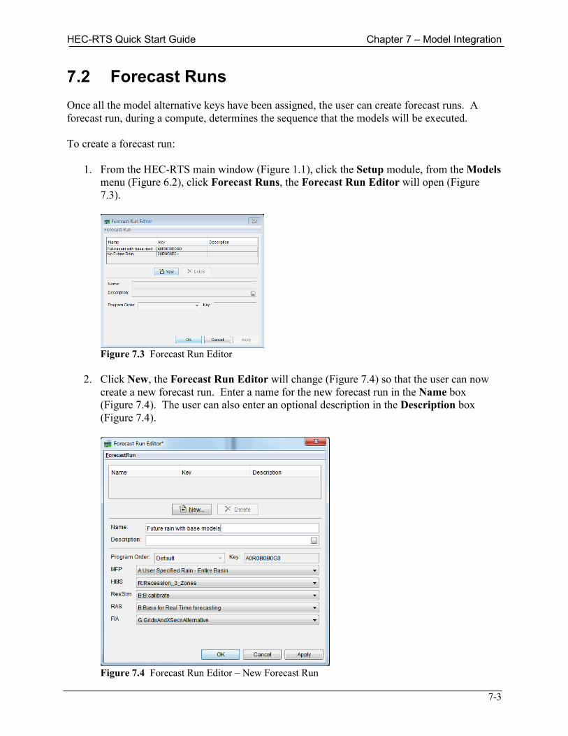
HEC-RTS Quick Start Guide Chapter 7 – Model Integration
7-3
Forecast Runs Once all the model alternative keys have been assigned, the user can create forecast runs. A forecast run, during a compute, determines the sequence that the models will be executed. To create a forecast run: 1. From the HEC-RTS main window (Figure 1.1), click the Setup module, from the Models
menu (Figure 6.2), click Forecast Runs, the Forecast Run Editor will open (Figure 7.3).
Figure 7.3 Forecast Run Editor
2. Click New, the Forecast Run Editor will change (Figure 7.4) so that the user can now
create a new forecast run. Enter a name for the new forecast run in the Name box (Figure 7.4). The user can also enter an optional description in the Description box (Figure 7.4).
Figure 7.4 Forecast Run Editor – New Forecast Run
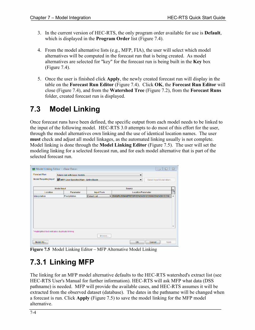
Chapter 7 – Model Integration HEC-RTS Quick Start Guide
7-4
3. In the current version of HEC-RTS, the only program order available for use is Default, which is displayed in the Program Order list (Figure 7.4).
4. From the model alternative lists (e.g., MFP, FIA), the user will select which model
alternatives will be computed in the forecast run that is being created. As model alternatives are selected for "key" for the forecast run is being built in the Key box (Figure 7.4).
5. Once the user is finished click Apply, the newly created forecast run will display in the
table on the Forecast Run Editor (Figure 7.4). Click OK, the Forecast Run Editor will close (Figure 7.4), and from the Watershed Tree (Figure 7.2), from the Forecast Runs folder, created forecast run is displayed.
Model Linking
Once forecast runs have been defined, the specific output from each model needs to be linked to the input of the following model. HEC-RTS 3.0 attempts to do most of this effort for the user, through the model alternatives own linking and the use of identical location names. The user must check and adjust all model linkages, as the automated linking usually is not complete. Model linking is done through the Model Linking Editor (Figure 7.5). The user will set the modeling linking for a selected forecast run, and for each model alternative that is part of the selected forecast run.
Figure 7.5 Model Linking Editor – MFP Alternative Model Linking 7.3.1 Linking MFP The linking for an MFP model alternative defaults to the HEC-RTS watershed's extract list (see HEC-RTS User's Manual for further information). HEC-RTS will ask MFP what data (DSS pathname) is needed. MFP will provide the available cases, and HEC-RTS assumes it will be extracted from the observed dataset (database). The dates in the pathname will be changed when a forecast is run. Click Apply (Figure 7.5) to save the model linking for the MFP model alternative.

HEC-RTS Quick Start Guide Chapter 7 – Model Integration
7-5
7.3.2 Linking HEC-HMS Before linking the HEC-HMS model alternatives, review Chapter 8 on the setting up and calibrating of the HEC-HMS model before beginning the linking process. In this case, Figure 7.6, for the HMS model alternative linking, all data, except for the precipitation from MFP will be extracted from the observed data (extract list). From the Input from column (Figure 7.6) for the Location – Interpolation (first row in the table), from the list, select the correct MFP model alternative (Figure 7.6). Validate the rest of the HMS model alternative linking, the user should be able to see right away the advantage of using consistent/identical location names throughout the system. Click Apply (Figure 7.6) to save the model linking for the HMS model alternative.
Figure 7.6 Model Linking Editor - HMS Alternative Model Linking 7.3.3 Linking HEC-ResSim In the example used in this manual, the ResSim model alternative will obtain most of the flows needed from the HMS model alternative, as well as some observed data (such as flows, storage elevations, etc.). Initially, the model linking for the ResSim model alternative defaults to the extract list (Figure 7.7). 1. From the table, highlight all of the locations, with the parameter Known Flow, click
Select Input Model Alternative (Figure 7.7), the Select Input Model Alternative dialog box will open (Figure 7.8).
2. From the Input Model Alternative list (Figure 7.8), select the correct HMS model
alternative. Click OK, the Select Input Model Alternative dialog box will close (Figure 7.8), and a Confirm Input Selection message window will appear (Figure 7.9). The message window is asking the user if this linking is appropriate for the selected rows. Click Yes, the Confirm Input Selection message window will close (Figure 7.9).
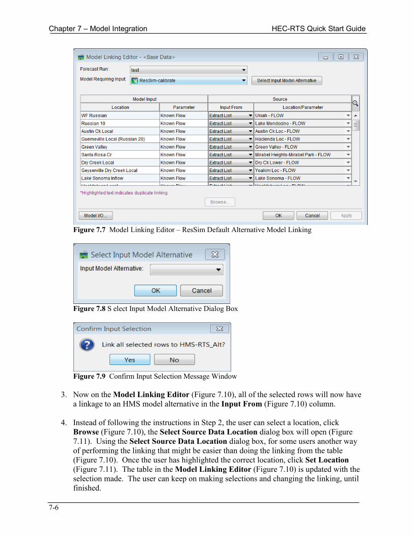
Chapter 7 – Model Integration HEC-RTS Quick Start Guide
7-6
Figure 7.7 Model Linking Editor – ResSim Default Alternative Model Linking
Figure 7.8 S elect Input Model Alternative Dialog Box
Figure 7.9 Confirm Input Selection Message Window
3. Now on the Model Linking Editor (Figure 7.10), all of the selected rows will now have
a linkage to an HMS model alternative in the Input From (Figure 7.10) column. 4. Instead of following the instructions in Step 2, the user can select a location, click
Browse (Figure 7.10), the Select Source Data Location dialog box will open (Figure 7.11). Using the Select Source Data Location dialog box, for some users another way of performing the linking that might be easier than doing the linking from the table (Figure 7.10). Once the user has highlighted the correct location, click Set Location (Figure 7.11). The table in the Model Linking Editor (Figure 7.10) is updated with the selection made. The user can keep on making selections and changing the linking, until finished.

HEC-RTS Quick Start Guide Chapter 7 – Model Integration
7-7
Figure 7.10 Model Linking Editor – ResSim Alternative Model Linking
Figure 7.11 Select Source Data Location Dialog Box
5. The user should review the ResSim model linking to check that the correct location and
parameter has been selected. HEC-RTS will do the best it can to match datasets, but if location names are not the same, then HEC-RTS tries to match items, and sometimes the software does not select correctly. HEC-RTS does try to help the user, by highlighting items in purple when the software thinks there is a duplicate linking (Figure 7.10).
6. Once the user has verified the linking for the ResSim model alternative, click Apply
(Figure 7.10) to save the model linking for the ResSim model alternative.
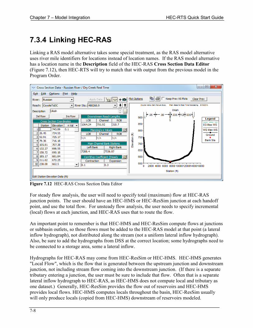
Chapter 7 – Model Integration HEC-RTS Quick Start Guide
7-8
7.3.4 Linking HEC-RAS Linking a RAS model alternative takes some special treatment, as the RAS model alternative uses river mile identifiers for locations instead of location names. If the RAS model alternative has a location name in the Description field of the HEC-RAS Cross Section Data Editor (Figure 7.12), then HEC-RTS will try to match that with output from the previous model in the Program Order.
Figure 7.12 HEC-RAS Cross Section Data Editor For steady flow analysis, the user will need to specify total (maximum) flow at HEC-RAS junction points. The user should have an HEC-HMS or HEC-ResSim junction at each handoff point, and use the total flow. For unsteady flow analysis, the user needs to specify incremental (local) flows at each junction, and HEC-RAS uses that to route the flow. An important point to remember is that HEC-HMS and HEC-ResSim compute flows at junctions or subbasin outlets, so those flows must be added to the HEC-RAS model at that point (a lateral inflow hydrograph), not distributed along the stream (not a uniform lateral inflow hydrograph). Also, be sure to add the hydrographs from DSS at the correct location; some hydrographs need to be connected to a storage area, some a lateral inflow. Hydrographs for HEC-RAS may come from HEC-ResSim or HEC-HMS. HEC-HMS generates "Local Flow", which is the flow that is generated between the upstream junction and downstream junction, not including stream flow coming into the downstream junction. (If there is a separate tributary entering a junction, the user must be sure to include that flow. Often that is a separate lateral inflow hydrograph to HEC-RAS, as HEC-HMS does not compute local and tributary as one dataset.) Generally, HEC-ResSim provides the flow out of reservoirs and HEC-HMS provides local flows. HEC-HMS computes locals throughout the basin, HEC-ResSim usually will only produce locals (copied from HEC-HMS) downstream of reservoirs modeled.
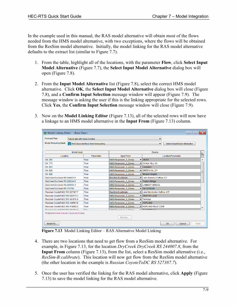
HEC-RTS Quick Start Guide Chapter 7 – Model Integration
7-9
In the example used in this manual, the RAS model alternative will obtain most of the flows needed from the HMS model alternative, with two exceptions, where the flows will be obtained from the ResSim model alternative. Initially, the model linking for the RAS model alternative defaults to the extract list (similar to Figure 7.7). 1. From the table, highlight all of the locations, with the parameter Flow, click Select Input
Model Alternative (Figure 7.7), the Select Input Model Alternative dialog box will open (Figure 7.8).
2. From the Input Model Alternative list (Figure 7.8), select the correct HMS model
alternative. Click OK, the Select Input Model Alternative dialog box will close (Figure 7.8), and a Confirm Input Selection message window will appear (Figure 7.9). The message window is asking the user if this is the linking appropriate for the selected rows. Click Yes, the Confirm Input Selection message window will close (Figure 7.9).
3. Now on the Model Linking Editor (Figure 7.13), all of the selected rows will now have
a linkage to an HMS model alternative in the Input From (Figure 7.13) column.
Figure 7.13 Model Linking Editor – RAS Alternative Model Linking
4. There are two locations that need to get flow from a ResSim model alternative. For
example, in Figure 7.13, for the location DryCreek DryCreek RS 244007.8, from the Input From column (Figure 7.13), from the list, select a ResSim model alternative (i.e., ResSim-B:calibrate). This location will now get flow from the ResSim model alternative (the other location in the example is Russian CoyoteToDC RS 527387.7).
5. Once the user has verified the linking for the RAS model alternative, click Apply (Figure
7.13) to save the model linking for the RAS model alternative.

Chapter 7 – Model Integration HEC-RTS Quick Start Guide
7-10
7.3.5 Linking HEC-FIA A FIA model alternative is usually built with using a RAS model alternative for the stage needed by the FIA model alternative to compute damage. Initially, the model linking for the FIA model alternative defaults to the extract list (similar to Figure 7.7). 1. From the Model Linking Editor (Figure 7.13), click Select Input Model Alternative
(Figure 7.7), the Select Input Model Alternative dialog box will open (Figure 7.8). 2. From the Input Model Alternative list (Figure 7.8), select the correct RAS model
alternative. Click OK, the Select Input Model Alternative dialog box will close (Figure 7.8), and a Confirm Input Selection message window will appear (Figure 7.9). The message window is asking the user if this linking is appropriate for the selected rows. Click Yes, the Confirm Input Selection message window will close (Figure 7.9).
3. Now on the Model Linking Editor (Figure 7.14), all of the selected rows will now have
a linkage to a RAS model alternative in the Input From (Figure 7.14) column.
Figure 7.14 Model Linking Editor – FIA Alternative Model Linking
4. Once the user has verified the linking for the FIA model alternative, click Apply (Figure
7.14) to save the model linking for the FIA model alternative.
Extract Setup The next step requires a watershed database to be setup and that contains data that will be used to make a forecast. Obtaining data will be different for each watershed and user base. Because of that, the setup process is discussed later in Chapter 9 of this manual, as well as chapter 18 of the HEC-RTS User's Manual. After the model alternatives have been linked together, the user needs
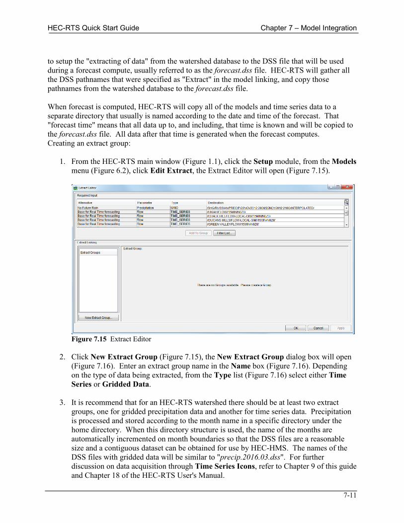
HEC-RTS Quick Start Guide Chapter 7 – Model Integration
7-11
to setup the "extracting of data" from the watershed database to the DSS file that will be used during a forecast compute, usually referred to as the forecast.dss file. HEC-RTS will gather all the DSS pathnames that were specified as "Extract" in the model linking, and copy those pathnames from the watershed database to the forecast.dss file. When forecast is computed, HEC-RTS will copy all of the models and time series data to a separate directory that usually is named according to the date and time of the forecast. That "forecast time" means that all data up to, and including, that time is known and will be copied to the forecast.dss file. All data after that time is generated when the forecast computes. Creating an extract group: 1. From the HEC-RTS main window (Figure 1.1), click the Setup module, from the Models
menu (Figure 6.2), click Edit Extract, the Extract Editor will open (Figure 7.15).
Figure 7.15 Extract Editor
2. Click New Extract Group (Figure 7.15), the New Extract Group dialog box will open
(Figure 7.16). Enter an extract group name in the Name box (Figure 7.16). Depending on the type of data being extracted, from the Type list (Figure 7.16) select either Time Series or Gridded Data.
3. It is recommend that for an HEC-RTS watershed there should be at least two extract
groups, one for gridded precipitation data and another for time series data. Precipitation is processed and stored according to the month name in a specific directory under the home directory. When this directory structure is used, the name of the months are automatically incremented on month boundaries so that the DSS files are a reasonable size and a contiguous dataset can be obtained for use by HEC-HMS. The names of the DSS files with gridded data will be similar to "precip.2016.03.dss". For further discussion on data acquisition through Time Series Icons, refer to Chapter 9 of this guide and Chapter 18 of the HEC-RTS User's Manual.
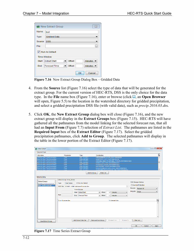
Chapter 7 – Model Integration HEC-RTS Quick Start Guide
7-12
Figure 7.16 New Extract Group Dialog Box – Gridded Data
4. From the Source list (Figure 7.16) select the type of data that will be generated for the
extract group. For the current version of HEC-RTS, DSS is the only choice for the data type. In the File name box (Figure 7.16), enter or browse (click , an Open Browser will open, Figure 5.5) to the location in the watershed directory for gridded precipitation, and select a gridded precipitation DSS file (with valid data), such as precip.2016.03.dss.
5. Click OK, the New Extract Group dialog box will close (Figure 7.16), and the new
extract group will display in the Extract Groups box (Figure 7.15). HEC-RTS will have gathered all the pathnames from the model linking for the selected forecast run, that all had an Input From (Figure 7.7) selection of Extract List. The pathnames are listed in the Required Input box of the Extract Editor (Figure 7.17). Select the gridded precipitation pathnames, click Add to Group. The selected pathnames will display in the table in the lower portion of the Extract Editor (Figure 7.17).
Figure 7.17 Time Series Extract Group
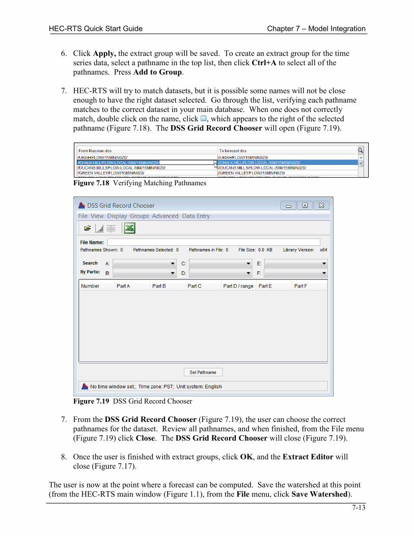
HEC-RTS Quick Start Guide Chapter 7 – Model Integration
7-13
6. Click Apply, the extract group will be saved. To create an extract group for the time series data, select a pathname in the top list, then click Ctrl+A to select all of the pathnames. Press Add to Group.
7. HEC-RTS will try to match datasets, but it is possible some names will not be close
enough to have the right dataset selected. Go through the list, verifying each pathname matches to the correct dataset in your main database. When one does not correctly match, double click on the name, click , which appears to the right of the selected pathname (Figure 7.18). The DSS Grid Record Chooser will open (Figure 7.19).
Figure 7.18 Verifying Matching Pathnames
Figure 7.19 DSS Grid Record Chooser
7. From the DSS Grid Record Chooser (Figure 7.19), the user can choose the correct
pathnames for the dataset. Review all pathnames, and when finished, from the File menu (Figure 7.19) click Close. The DSS Grid Record Chooser will close (Figure 7.19).
8. Once the user is finished with extract groups, click OK, and the Extract Editor will
close (Figure 7.17). The user is now at the point where a forecast can be computed. Save the watershed at this point (from the HEC-RTS main window (Figure 1.1), from the File menu, click Save Watershed).
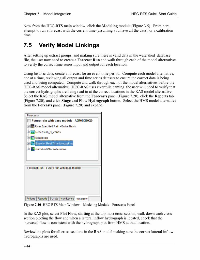
Chapter 7 – Model Integration HEC-RTS Quick Start Guide
7-14
Now from the HEC-RTS main window, click the Modeling module (Figure 3.5). From here, attempt to run a forecast with the current time (assuming you have all the data), or a calibration time.
Verify Model Linkings After setting up extract groups, and making sure there is valid data in the watershed database file, the user now need to create a Forecast Run and walk through each of the model alternatives to verify the correct time series input and output for each location. Using historic data, create a forecast for an event time period. Compute each model alternative, one at a time, reviewing all output and time series datasets to ensure the correct data is being used and being computed. Compute and walk through each of the model alternatives before the HEC-RAS model alternative. HEC-RAS uses rivermile naming, the user will need to verify that the correct hydrographs are being read in at the correct locations in the RAS model alternative. Select the RAS model alternative from the Forecasts panel (Figure 7.20), click the Reports tab (Figure 7.20), and click Stage and Flow Hydrograph button. Select the HMS model alternative from the Forcasts panel (Figure 7.20) and expand.
Figure 7.20 HEC-RTS Main Window – Modeling Module - Forecasts Panel In the RAS plot, select Plot Flow, starting at the top most cross section, walk down each cross section plotting the flow and when a latteral inflow hydrograph is located, check that the increased flow is consistent with the hydrograph plot from HMS at that location. Review the plots for all cross sections in the RAS model making sure the correct latteral inflow hydrographs are used.
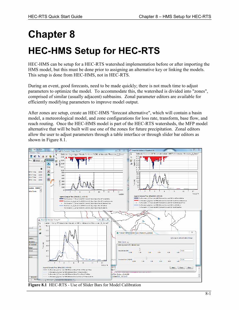
HEC-RTS Quick Start Guide Chapter 8 – HMS Setup for HEC-RTS
8-1
HEC-HMS Setup for HEC-RTS HEC-HMS can be setup for a HEC-RTS watershed implementation before or after importing the HMS model, but this must be done prior to assigning an alternative key or linking the models. This setup is done from HEC-HMS, not in HEC-RTS. During an event, good forecasts, need to be made quickly; there is not much time to adjust parameters to optimize the model. To accommodate this, the watershed is divided into "zones", comprised of similar (usually adjacent) subbasins. Zonal parameter editors are available for efficiently modifying parameters to improve model output. After zones are setup, create an HEC-HMS "forecast alternative", which will contain a basin model, a meteorological model, and zone configurations for loss rate, transform, base flow, and reach routing. Once the HEC-HMS model is part of the HEC-RTS watersheds, the MFP model alternative that will be built will use one of the zones for future precipitation. Zonal editors allow the user to adjust parameters through a table interface or through slider bar editors as shown in Figure 8.1.
Figure 8.1 HEC-RTS - Use of Slider Bars for Model Calibration

Chapter 8 – HMS Setup for HEC-RTS HEC-RTS Quick Start Guide
8-2
Zone Configuration A zone configuration will be applied to the HEC-HMS model based on subbasin locations. Generally, parameters are adjusted for all subbasins within a zone. The user can set each parameter to a specific number for a zone, or multiply/divide the parameter for each subbasin within a zone by a constant, or add/subtract a constant to each parameter for each subbasin, or set the parameter for individual subbasins to specific values. Refer to the HEC-HMS user’s manual for a description of setting up zones and configuring a forecast alternative. For future precipitation, the amount of precipitation is set for the entire zone, and can be specified as a temporal distribution for each zone. The user can also multiply observed precipitation by a percentage for each zone.
Defining Zones Define zone in the HEC-HMS model: 1. From the HEC-HMS main window (Figure 8.2), from the Parameters menu, click Zone
Configuration Manager, the Zone Configuration Manager will open (Figure 8.3).
Figure 8.2 HEC-HMS Main Window – Parameters Menu
Figure 8.3 HEC-HMS – Zone Configuration Manager
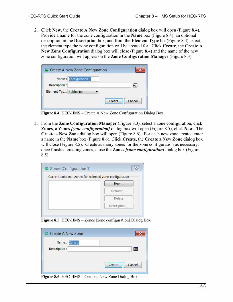
HEC-RTS Quick Start Guide Chapter 8 – HMS Setup for HEC-RTS
8-3
2. Click New, the Create A New Zone Configuration dialog box will open (Figure 8.4). Provide a name for the zone configuration in the Name box (Figure 8.4), an optional description in the Description box, and from the Element Type list (Figure 8.4) select the element type the zone configuration will be created for. Click Create, the Create A New Zone Configuration dialog box will close (Figure 8.4) and the name of the new zone configuration will appear on the Zone Configuration Manager (Figure 8.3).
Figure 8.4 HEC-HMS – Create A New Zone Configuration Dialog Box
3. From the Zone Configuration Manager (Figure 8.3), select a zone configuration, click
Zones, a Zones [zone configuration] dialog box will open (Figure 8.5), click New. The Create a New Zone dialog box will open (Figure 8.6). For each new zone created enter a name in the Name box (Figure 8.6). Click Create, the Create a New Zone dialog box will close (Figure 8.5). Create as many zones for the zone configuration as necessary, once finished creating zones, close the Zones [zone configuration] dialog box (Figure 8.5).
Figure 8.5 HEC-HMS – Zones [zone configuration] Dialog Box
Figure 8.6 HEC-HMS – Create a New Zone Dialog Box
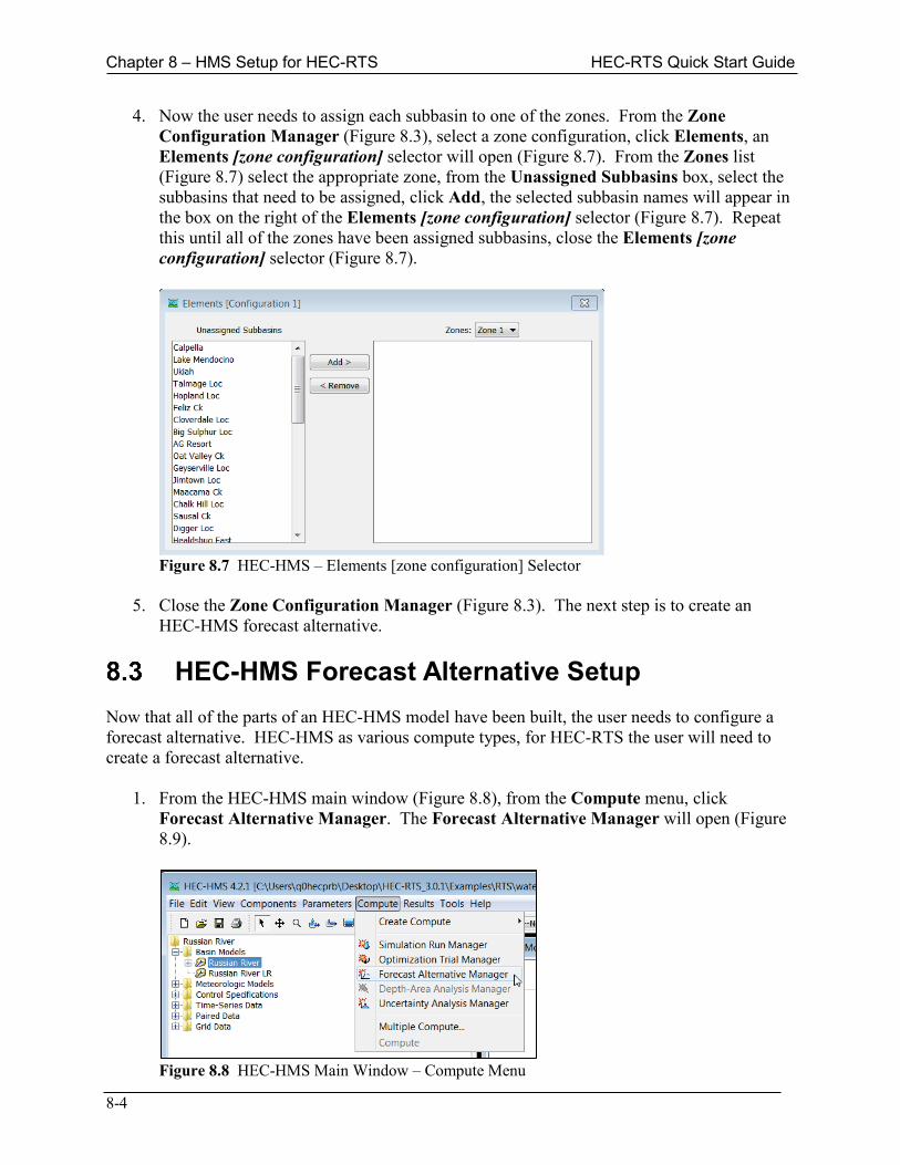
Chapter 8 – HMS Setup for HEC-RTS HEC-RTS Quick Start Guide
8-4
4. Now the user needs to assign each subbasin to one of the zones. From the Zone Configuration Manager (Figure 8.3), select a zone configuration, click Elements, an Elements [zone configuration] selector will open (Figure 8.7). From the Zones list (Figure 8.7) select the appropriate zone, from the Unassigned Subbasins box, select the subbasins that need to be assigned, click Add, the selected subbasin names will appear in the box on the right of the Elements [zone configuration] selector (Figure 8.7). Repeat this until all of the zones have been assigned subbasins, close the Elements [zone configuration] selector (Figure 8.7).
Figure 8.7 HEC-HMS – Elements [zone configuration] Selector
5. Close the Zone Configuration Manager (Figure 8.3). The next step is to create an
HEC-HMS forecast alternative.
HEC-HMS Forecast Alternative Setup Now that all of the parts of an HEC-HMS model have been built, the user needs to configure a forecast alternative. HEC-HMS as various compute types, for HEC-RTS the user will need to create a forecast alternative. 1. From the HEC-HMS main window (Figure 8.8), from the Compute menu, click
Forecast Alternative Manager. The Forecast Alternative Manager will open (Figure 8.9).
Figure 8.8 HEC-HMS Main Window – Compute Menu
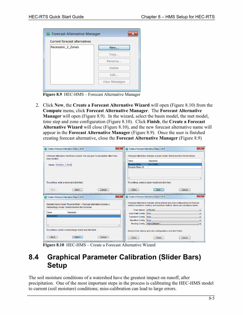
HEC-RTS Quick Start Guide Chapter 8 – HMS Setup for HEC-RTS
8-5
Figure 8.9 HEC-HMS – Forecast Alternative Manager
2. Click New, the Create a Forecast Alternative Wizard will open (Figure 8.10) from the
Compute menu, click Forecast Alternative Manager. The Forecast Alternative Manager will open (Figure 8.9). In the wizard, select the basin model, the met model, time step and zone configuration (Figure 8.10). Click Finish, the Create a Forecast Alternative Wizard will close (Figure 8.10), and the new forecast alternative name will appear in the Forecast Alternative Manager (Figure 8.9). Once the user is finished creating forecast alternative, close the Forecast Alternative Manager (Figure 8.9)
Figure 8.10 HEC-HMS – Create a Forecast Alternative Wizard
Graphical Parameter Calibration (Slider Bars)
Setup The soil moisture conditions of a watershed have the greatest impact on runoff, after precipitation. One of the most important steps in the process is calibrating the HEC-HMS model to current (soil moisture) conditions; miss-calibration can lead to large errors.
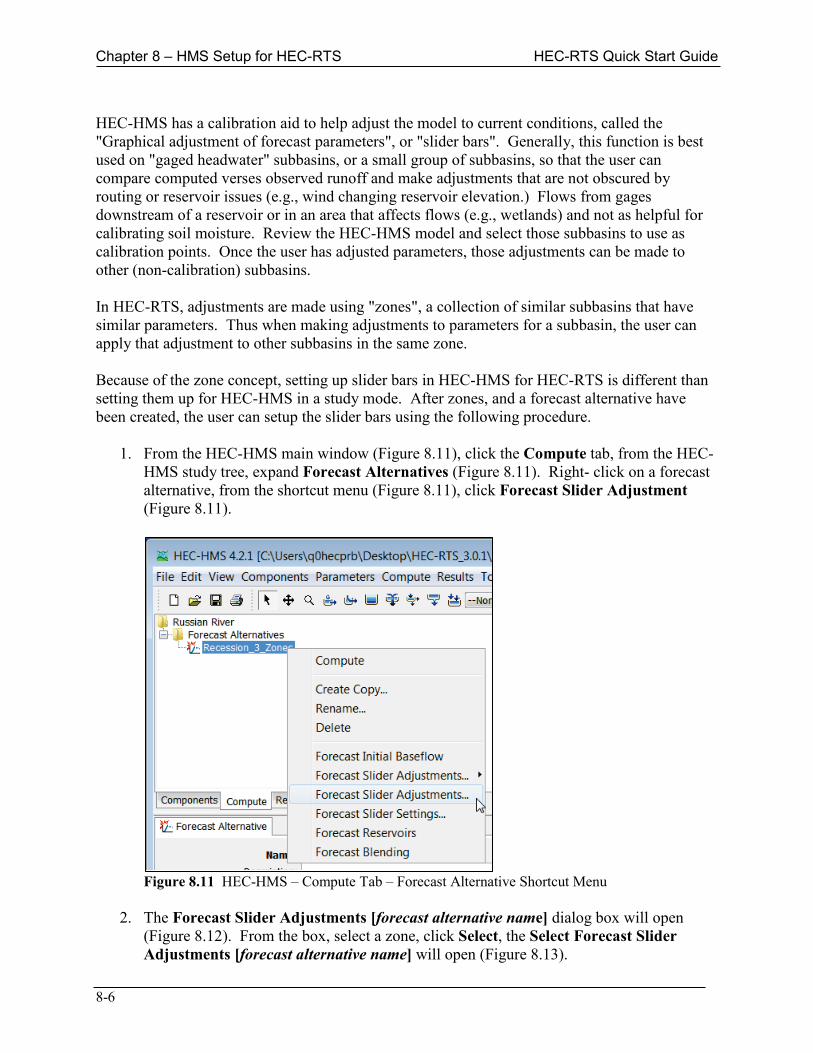
Chapter 8 – HMS Setup for HEC-RTS HEC-RTS Quick Start Guide
8-6
HEC-HMS has a calibration aid to help adjust the model to current conditions, called the "Graphical adjustment of forecast parameters", or "slider bars". Generally, this function is best used on "gaged headwater" subbasins, or a small group of subbasins, so that the user can compare computed verses observed runoff and make adjustments that are not obscured by routing or reservoir issues (e.g., wind changing reservoir elevation.) Flows from gages downstream of a reservoir or in an area that affects flows (e.g., wetlands) and not as helpful for calibrating soil moisture. Review the HEC-HMS model and select those subbasins to use as calibration points. Once the user has adjusted parameters, those adjustments can be made to other (non-calibration) subbasins. In HEC-RTS, adjustments are made using "zones", a collection of similar subbasins that have similar parameters. Thus when making adjustments to parameters for a subbasin, the user can apply that adjustment to other subbasins in the same zone. Because of the zone concept, setting up slider bars in HEC-HMS for HEC-RTS is different than setting them up for HEC-HMS in a study mode. After zones, and a forecast alternative have been created, the user can setup the slider bars using the following procedure. 1. From the HEC-HMS main window (Figure 8.11), click the Compute tab, from the HEC-
HMS study tree, expand Forecast Alternatives (Figure 8.11). Right- click on a forecast alternative, from the shortcut menu (Figure 8.11), click Forecast Slider Adjustment (Figure 8.11).
Figure 8.11 HEC-HMS – Compute Tab – Forecast Alternative Shortcut Menu
2. The Forecast Slider Adjustments [forecast alternative name] dialog box will open
(Figure 8.12). From the box, select a zone, click Select, the Select Forecast Slider Adjustments [forecast alternative name] will open (Figure 8.13).
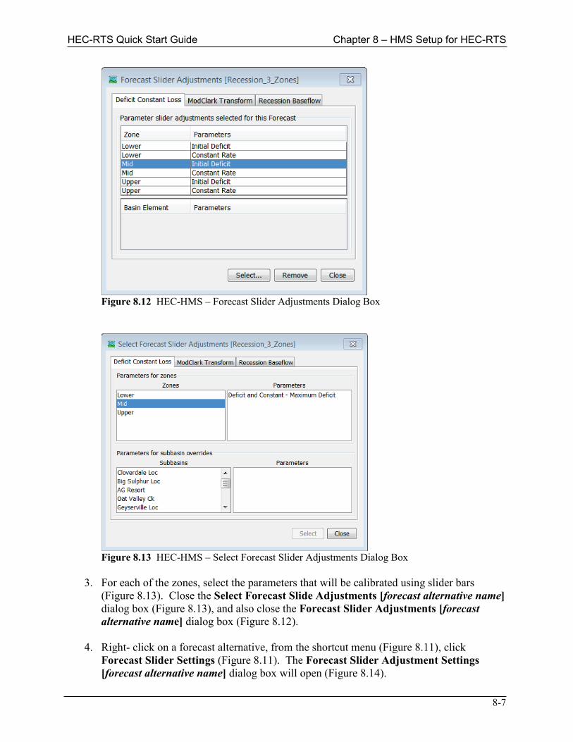
HEC-RTS Quick Start Guide Chapter 8 – HMS Setup for HEC-RTS
8-7
Figure 8.12 HEC-HMS – Forecast Slider Adjustments Dialog Box
Figure 8.13 HEC-HMS – Select Forecast Slider Adjustments Dialog Box
3. For each of the zones, select the parameters that will be calibrated using slider bars
(Figure 8.13). Close the Select Forecast Slide Adjustments [forecast alternative name] dialog box (Figure 8.13), and also close the Forecast Slider Adjustments [forecast alternative name] dialog box (Figure 8.12).
4. Right- click on a forecast alternative, from the shortcut menu (Figure 8.11), click
Forecast Slider Settings (Figure 8.11). The Forecast Slider Adjustment Settings [forecast alternative name] dialog box will open (Figure 8.14).

Chapter 8 – HMS Setup for HEC-RTS HEC-RTS Quick Start Guide
8-8
Figure 8.14 HEC-HMS – Forecast Slider Adjustments Settings [forecast alternative name]
Dialog Box 5. Adjust the maximum and minimum possible parameter values, as appropriate. When
finished with adjustments click Apply, click Close, the Forecast Slider Adjustment Settings [forecast alternative name] dialog box will close (Figure 8.14).
Now the user has finished making all the necessary setup and adjustments needed to the HEC-HMS model. 1. From the HEC-RTS main window, from the Modeling module (Figure 8.15), open a
forecast, from the Forecasts box, select the HMS model alternative. Click the Actions tab (Figure 8.15), click Combined Parameter Editor, a Forecast [forecast name] editor will open (Figure 8.16).
Figure 8.15 HEC-RTS – Modeling Module – Actions Tab
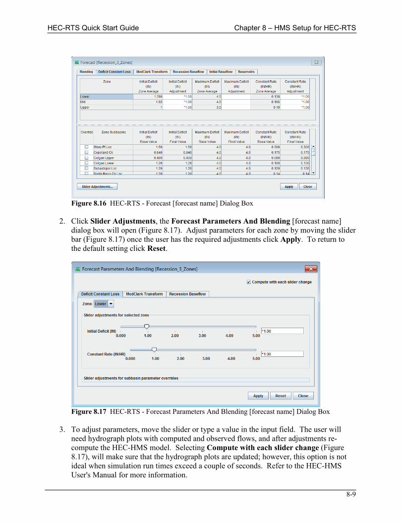
HEC-RTS Quick Start Guide Chapter 8 – HMS Setup for HEC-RTS
8-9
Figure 8.16 HEC-RTS - Forecast [forecast name] Dialog Box
2. Click Slider Adjustments, the Forecast Parameters And Blending [forecast name] dialog box will open (Figure 8.17). Adjust parameters for each zone by moving the slider bar (Figure 8.17) once the user has the required adjustments click Apply. To return to the default setting click Reset.
Figure 8.17 HEC-RTS - Forecast Parameters And Blending [forecast name] Dialog Box
3. To adjust parameters, move the slider or type a value in the input field. The user will
need hydrograph plots with computed and observed flows, and after adjustments re-compute the HEC-HMS model. Selecting Compute with each slider change (Figure 8.17), will make sure that the hydrograph plots are updated; however, this option is not ideal when simulation run times exceed a couple of seconds. Refer to the HEC-HMS User's Manual for more information.

Chapter 8 – HMS Setup for HEC-RTS HEC-RTS Quick Start Guide
8-10
4. When the user is finished with all adjustments click Close, the Forecast Parameters And Blending [forecast name] dialog box will close (Figure 8.17).
HEC-RTS Quick Start Guide Chapter 9 – Time Series Icons
9-1
Time Series Icons Time series icons provide access to observed and computed time series and paired data. The data may be either from a DSS file, websites, webcams, scripts, spreadsheets, or other files. Time series data can appear as thumbnail plots or color bars. The icons provide easy access for analyzing data and providing location-specific information (e.g., frequently updated pictures of gages, reports on the location). In addition, datasets may be set to display by turning on or off Time Series Layers (Figure 5.9), a subcomponent of map layers. Example layers include: Flow, Stage, Precip, and Modeled Results. Selecting a specific layer allows the user to view certain data types and remove clutter from a map window. Setting up the layers first, and then adding icon datasets to the layers is the recommend way for setting up time series icons. Of course, the watershed database needs to be populated with data before creating time series icons.
Time Series Layers The Time Series Icons Layer (Figure 5.9) is a default map layer, with the user defining the different specific time series layers. A time series layer is used to display a specific type of data, such as all flow gages, or computed stages. The user can also organize the defined time series layers, for example:
• All • Flow • Stage • Precip • Elevation • Lakes • Modeled
Creating Time Series Layers
To create a time series layer: 1. From the HEC-RTS main window (Figure 5.1), click the Setup module, from the Maps
menu, click Map Layers. The Map Layers dialog box (Figure 5.2) will open, right click on Time Series Icons, from the shortcut menu (Figure 9.1), and click Add Icon Layer.
2. The New Time Series Icon Layer dialog box will open (Figure 9.2). Enter a name in the
Name box (e.g., Flow, Stage, or Precip). The user may enter an optional description in
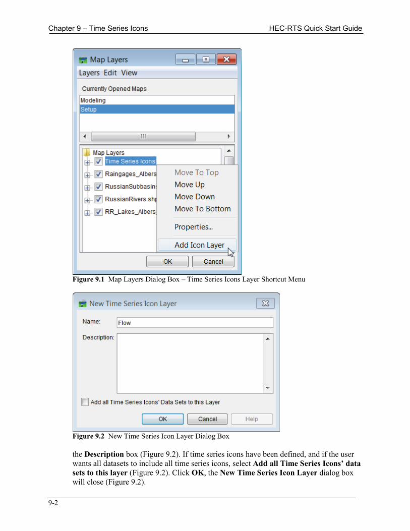
Chapter 9 – Time Series Icons HEC-RTS Quick Start Guide
9-2
Figure 9.1 Map Layers Dialog Box – Time Series Icons Layer Shortcut Menu
Figure 9.2 New Time Series Icon Layer Dialog Box
the Description box (Figure 9.2). If time series icons have been defined, and if the user
wants all datasets to include all time series icons, select Add all Time Series Icons’ data sets to this layer (Figure 9.2). Click OK, the New Time Series Icon Layer dialog box will close (Figure 9.2).
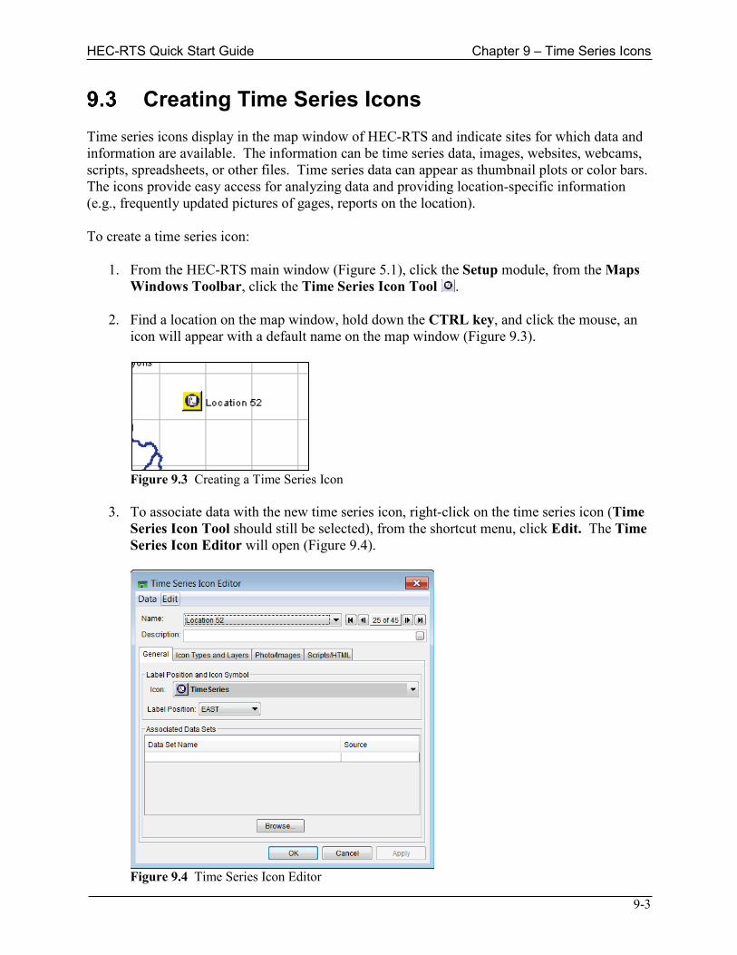
HEC-RTS Quick Start Guide Chapter 9 – Time Series Icons
9-3
Creating Time Series Icons Time series icons display in the map window of HEC-RTS and indicate sites for which data and information are available. The information can be time series data, images, websites, webcams, scripts, spreadsheets, or other files. Time series data can appear as thumbnail plots or color bars. The icons provide easy access for analyzing data and providing location-specific information (e.g., frequently updated pictures of gages, reports on the location). To create a time series icon: 1. From the HEC-RTS main window (Figure 5.1), click the Setup module, from the Maps
Windows Toolbar, click the Time Series Icon Tool . 2. Find a location on the map window, hold down the CTRL key, and click the mouse, an
icon will appear with a default name on the map window (Figure 9.3).
Figure 9.3 Creating a Time Series Icon
3. To associate data with the new time series icon, right-click on the time series icon (Time
Series Icon Tool should still be selected), from the shortcut menu, click Edit. The Time Series Icon Editor will open (Figure 9.4).
Figure 9.4 Time Series Icon Editor
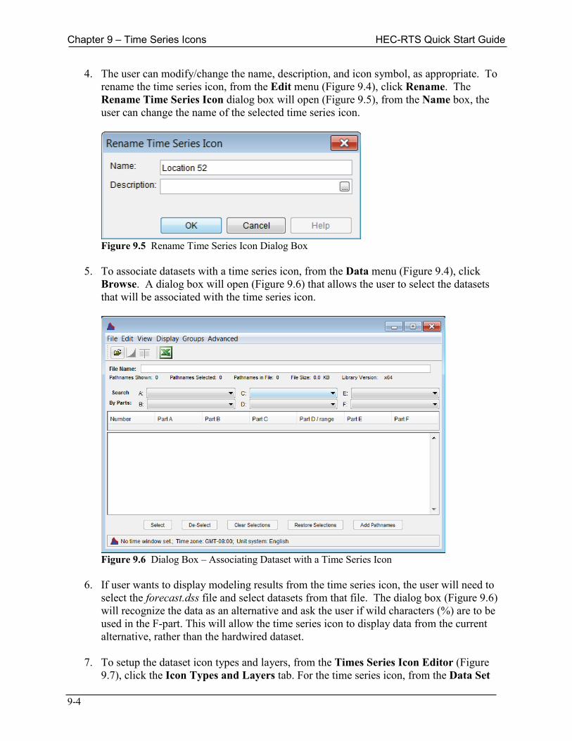
Chapter 9 – Time Series Icons HEC-RTS Quick Start Guide
9-4
4. The user can modify/change the name, description, and icon symbol, as appropriate. To rename the time series icon, from the Edit menu (Figure 9.4), click Rename. The Rename Time Series Icon dialog box will open (Figure 9.5), from the Name box, the user can change the name of the selected time series icon.
Figure 9.5 Rename Time Series Icon Dialog Box
5. To associate datasets with a time series icon, from the Data menu (Figure 9.4), click
Browse. A dialog box will open (Figure 9.6) that allows the user to select the datasets that will be associated with the time series icon.
Figure 9.6 Dialog Box – Associating Dataset with a Time Series Icon
6. If user wants to display modeling results from the time series icon, the user will need to
select the forecast.dss file and select datasets from that file. The dialog box (Figure 9.6) will recognize the data as an alternative and ask the user if wild characters (%) are to be used in the F-part. This will allow the time series icon to display data from the current alternative, rather than the hardwired dataset.
7. To setup the dataset icon types and layers, from the Times Series Icon Editor (Figure
9.7), click the Icon Types and Layers tab. For the time series icon, from the Data Set
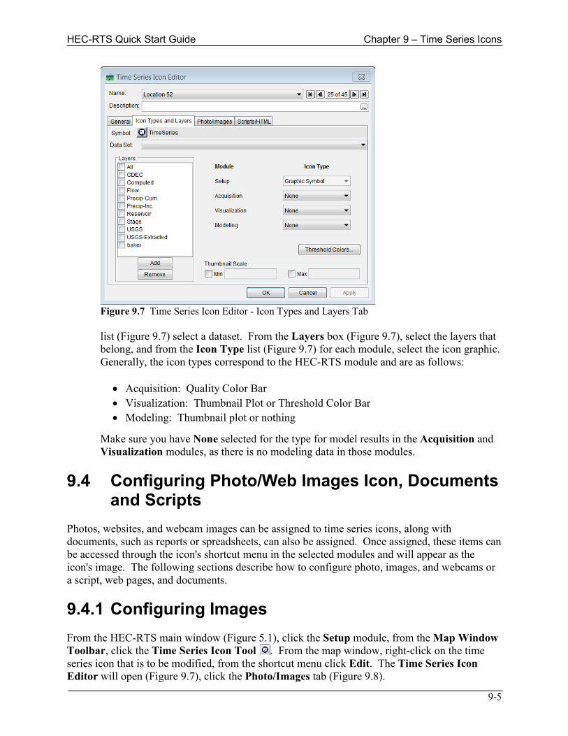
HEC-RTS Quick Start Guide Chapter 9 – Time Series Icons
9-5
Figure 9.7 Time Series Icon Editor - Icon Types and Layers Tab
list (Figure 9.7) select a dataset. From the Layers box (Figure 9.7), select the layers that
belong, and from the Icon Type list (Figure 9.7) for each module, select the icon graphic. Generally, the icon types correspond to the HEC-RTS module and are as follows:
• Acquisition: Quality Color Bar • Visualization: Thumbnail Plot or Threshold Color Bar • Modeling: Thumbnail plot or nothing
Make sure you have None selected for the type for model results in the Acquisition and Visualization modules, as there is no modeling data in those modules.
Configuring Photo/Web Images Icon, Documents
and Scripts Photos, websites, and webcam images can be assigned to time series icons, along with documents, such as reports or spreadsheets, can also be assigned. Once assigned, these items can be accessed through the icon's shortcut menu in the selected modules and will appear as the icon's image. The following sections describe how to configure photo, images, and webcams or a script, web pages, and documents. 9.4.1 Configuring Images From the HEC-RTS main window (Figure 5.1), click the Setup module, from the Map Window Toolbar, click the Time Series Icon Tool . From the map window, right-click on the time series icon that is to be modified, from the shortcut menu click Edit. The Time Series Icon Editor will open (Figure 9.7), click the Photo/Images tab (Figure 9.8).
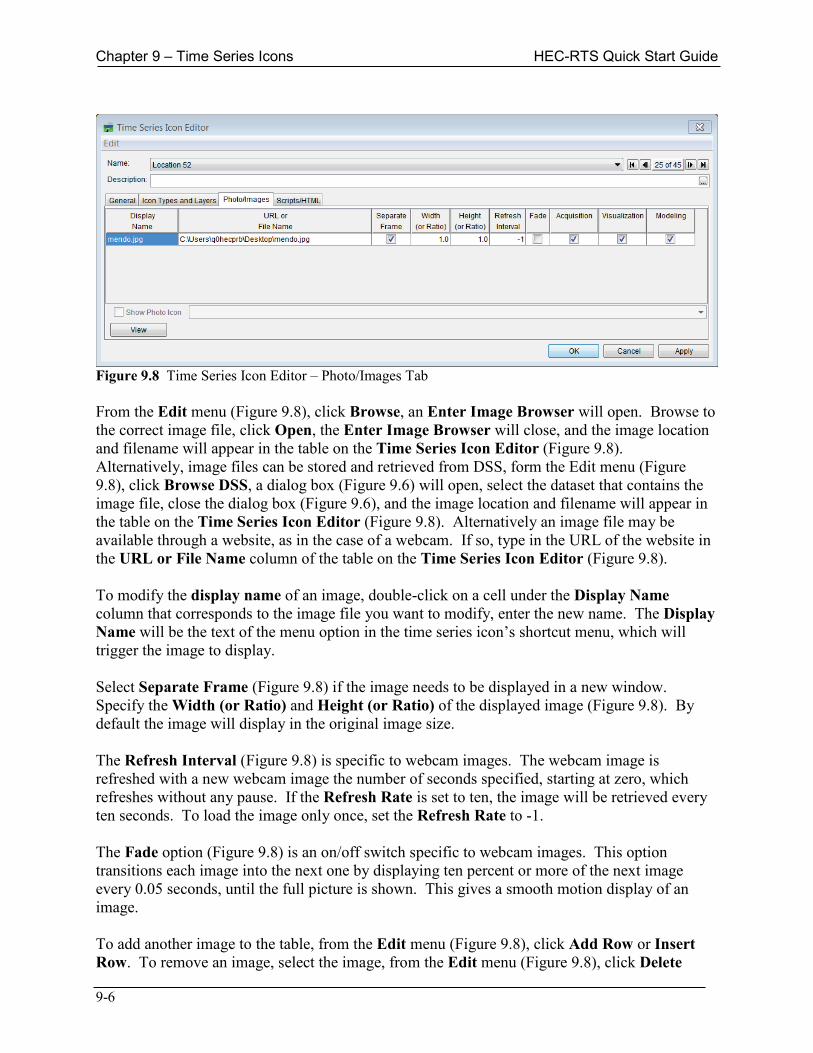
Chapter 9 – Time Series Icons HEC-RTS Quick Start Guide
9-6
Figure 9.8 Time Series Icon Editor – Photo/Images Tab From the Edit menu (Figure 9.8), click Browse, an Enter Image Browser will open. Browse to the correct image file, click Open, the Enter Image Browser will close, and the image location and filename will appear in the table on the Time Series Icon Editor (Figure 9.8). Alternatively, image files can be stored and retrieved from DSS, form the Edit menu (Figure 9.8), click Browse DSS, a dialog box (Figure 9.6) will open, select the dataset that contains the image file, close the dialog box (Figure 9.6), and the image location and filename will appear in the table on the Time Series Icon Editor (Figure 9.8). Alternatively an image file may be available through a website, as in the case of a webcam. If so, type in the URL of the website in the URL or File Name column of the table on the Time Series Icon Editor (Figure 9.8). To modify the display name of an image, double-click on a cell under the Display Name column that corresponds to the image file you want to modify, enter the new name. The Display Name will be the text of the menu option in the time series icon’s shortcut menu, which will trigger the image to display. Select Separate Frame (Figure 9.8) if the image needs to be displayed in a new window. Specify the Width (or Ratio) and Height (or Ratio) of the displayed image (Figure 9.8). By default the image will display in the original image size. The Refresh Interval (Figure 9.8) is specific to webcam images. The webcam image is refreshed with a new webcam image the number of seconds specified, starting at zero, which refreshes without any pause. If the Refresh Rate is set to ten, the image will be retrieved every ten seconds. To load the image only once, set the Refresh Rate to -1. The Fade option (Figure 9.8) is an on/off switch specific to webcam images. This option transitions each image into the next one by displaying ten percent or more of the next image every 0.05 seconds, until the full picture is shown. This gives a smooth motion display of an image. To add another image to the table, from the Edit menu (Figure 9.8), click Add Row or Insert Row. To remove an image, select the image, from the Edit menu (Figure 9.8), click Delete
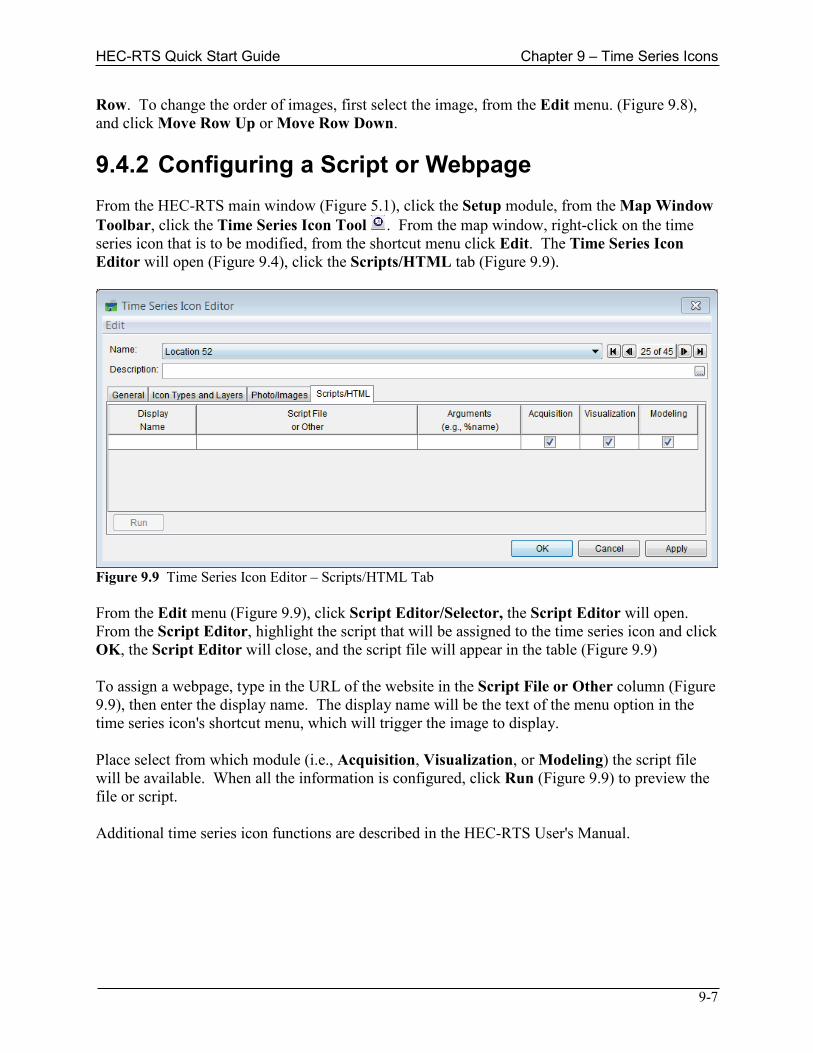
HEC-RTS Quick Start Guide Chapter 9 – Time Series Icons
9-7
Row. To change the order of images, first select the image, from the Edit menu. (Figure 9.8), and click Move Row Up or Move Row Down. 9.4.2 Configuring a Script or Webpage From the HEC-RTS main window (Figure 5.1), click the Setup module, from the Map Window Toolbar, click the Time Series Icon Tool . From the map window, right-click on the time series icon that is to be modified, from the shortcut menu click Edit. The Time Series Icon Editor will open (Figure 9.4), click the Scripts/HTML tab (Figure 9.9).
Figure 9.9 Time Series Icon Editor – Scripts/HTML Tab From the Edit menu (Figure 9.9), click Script Editor/Selector, the Script Editor will open. From the Script Editor, highlight the script that will be assigned to the time series icon and click OK, the Script Editor will close, and the script file will appear in the table (Figure 9.9) To assign a webpage, type in the URL of the website in the Script File or Other column (Figure 9.9), then enter the display name. The display name will be the text of the menu option in the time series icon's shortcut menu, which will trigger the image to display. Place select from which module (i.e., Acquisition, Visualization, or Modeling) the script file will be available. When all the information is configured, click Run (Figure 9.9) to preview the file or script. Additional time series icon functions are described in the HEC-RTS User's Manual.

Chapter 9 – Time Series Icons HEC-RTS Quick Start Guide
9-8
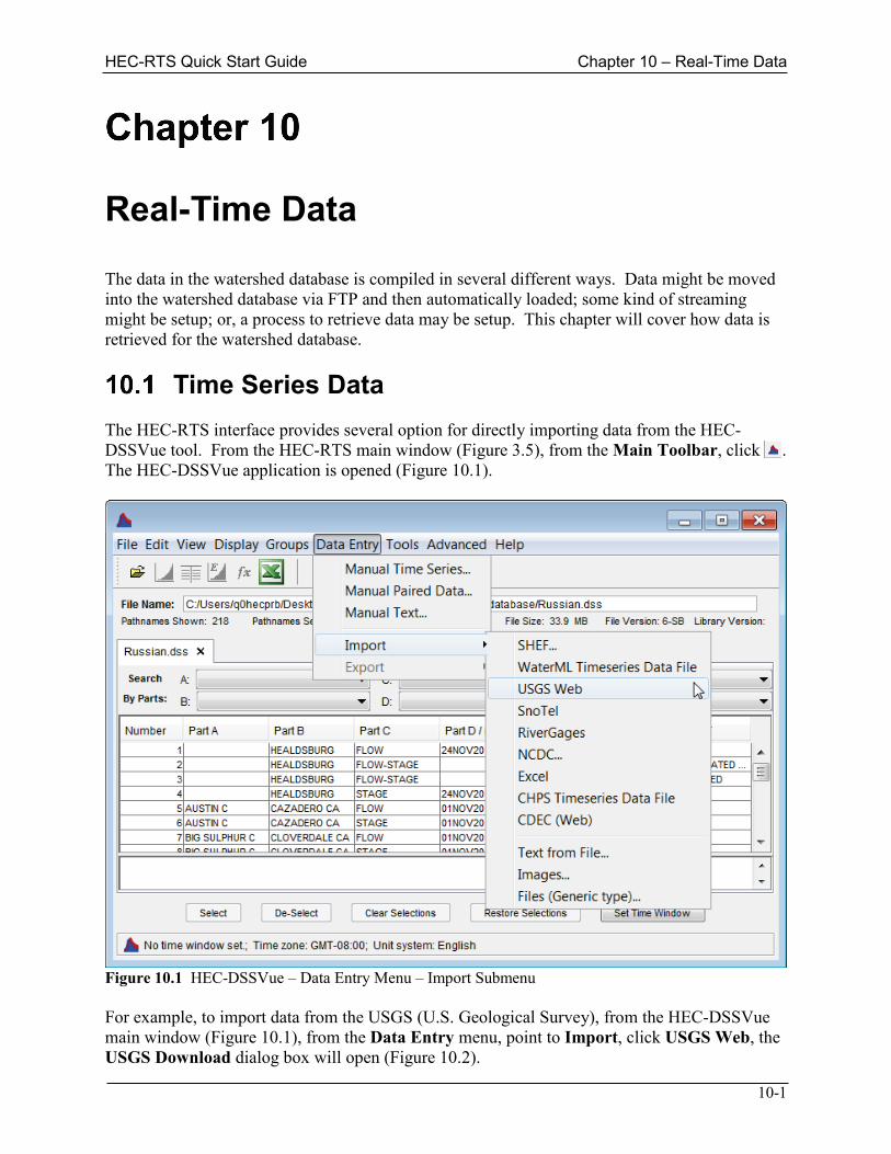
HEC-RTS Quick Start Guide Chapter 10 – Real-Time Data
10-1
Real-Time Data The data in the watershed database is compiled in several different ways. Data might be moved into the watershed database via FTP and then automatically loaded; some kind of streaming might be setup; or, a process to retrieve data may be setup. This chapter will cover how data is retrieved for the watershed database.
Time Series Data The HEC-RTS interface provides several option for directly importing data from the HEC-DSSVue tool. From the HEC-RTS main window (Figure 3.5), from the Main Toolbar, click . The HEC-DSSVue application is opened (Figure 10.1).
Figure 10.1 HEC-DSSVue – Data Entry Menu – Import Submenu For example, to import data from the USGS (U.S. Geological Survey), from the HEC-DSSVue main window (Figure 10.1), from the Data Entry menu, point to Import, click USGS Web, the USGS Download dialog box will open (Figure 10.2).
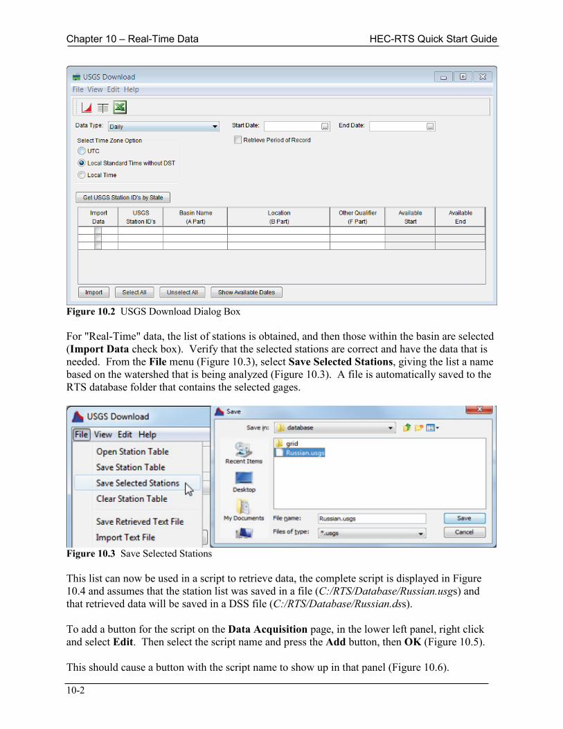
Chapter 10 – Real-Time Data HEC-RTS Quick Start Guide
10-2
Figure 10.2 USGS Download Dialog Box For "Real-Time" data, the list of stations is obtained, and then those within the basin are selected (Import Data check box). Verify that the selected stations are correct and have the data that is needed. From the File menu (Figure 10.3), select Save Selected Stations, giving the list a name based on the watershed that is being analyzed (Figure 10.3). A file is automatically saved to the RTS database folder that contains the selected gages.
Figure 10.3 Save Selected Stations This list can now be used in a script to retrieve data, the complete script is displayed in Figure 10.4 and assumes that the station list was saved in a file (C:/RTS/Database/Russian.usgs) and that retrieved data will be saved in a DSS file (C:/RTS/Database/Russian.dss). To add a button for the script on the Data Acquisition page, in the lower left panel, right click and select Edit. Then select the script name and press the Add button, then OK (Figure 10.5). This should cause a button with the script name to show up in that panel (Figure 10.6).
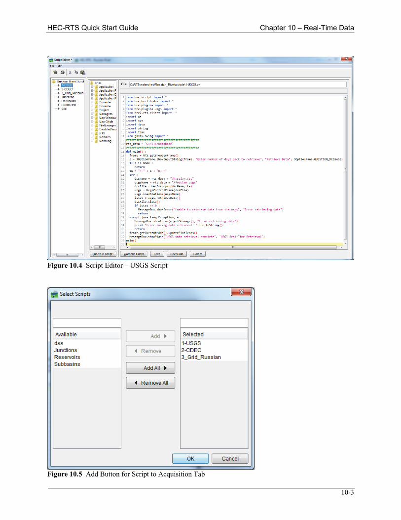
HEC-RTS Quick Start Guide Chapter 10 – Real-Time Data
10-3
Figure 10.4 Script Editor – USGS Script
Figure 10.5 Add Button for Script to Acquisition Tab
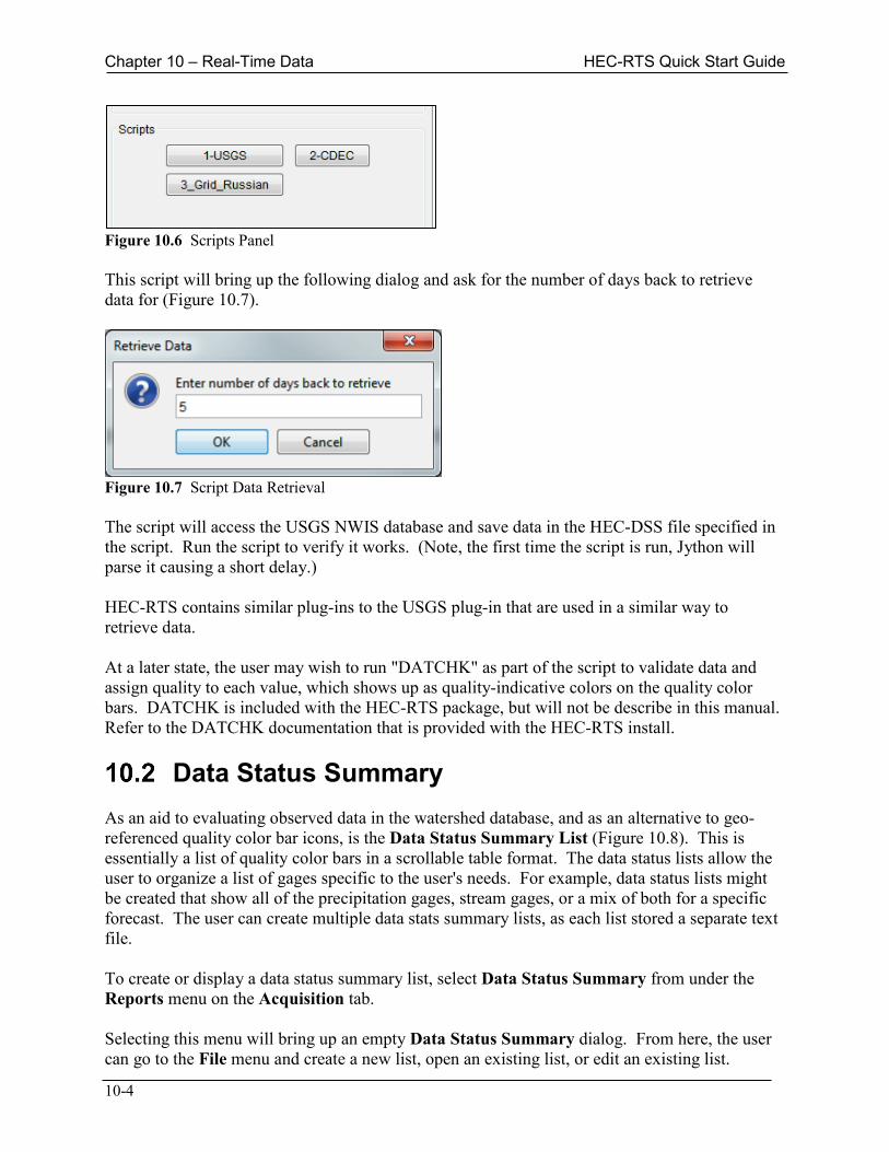
Chapter 10 – Real-Time Data HEC-RTS Quick Start Guide
10-4
Figure 10.6 Scripts Panel This script will bring up the following dialog and ask for the number of days back to retrieve data for (Figure 10.7).
Figure 10.7 Script Data Retrieval The script will access the USGS NWIS database and save data in the HEC-DSS file specified in the script. Run the script to verify it works. (Note, the first time the script is run, Jython will parse it causing a short delay.) HEC-RTS contains similar plug-ins to the USGS plug-in that are used in a similar way to retrieve data. At a later state, the user may wish to run "DATCHK" as part of the script to validate data and assign quality to each value, which shows up as quality-indicative colors on the quality color bars. DATCHK is included with the HEC-RTS package, but will not be describe in this manual. Refer to the DATCHK documentation that is provided with the HEC-RTS install.
Data Status Summary As an aid to evaluating observed data in the watershed database, and as an alternative to geo-referenced quality color bar icons, is the Data Status Summary List (Figure 10.8). This is essentially a list of quality color bars in a scrollable table format. The data status lists allow the user to organize a list of gages specific to the user's needs. For example, data status lists might be created that show all of the precipitation gages, stream gages, or a mix of both for a specific forecast. The user can create multiple data stats summary lists, as each list stored a separate text file. To create or display a data status summary list, select Data Status Summary from under the Reports menu on the Acquisition tab. Selecting this menu will bring up an empty Data Status Summary dialog. From here, the user can go to the File menu and create a new list, open an existing list, or edit an existing list.

HEC-RTS Quick Start Guide Chapter 10 – Real-Time Data
10-5
Generally, once datasets have been quality checked with DATCHK or similar, then the user can setup lists. Creating a Data Status Summary list is relatively easy. From the Edit menu, select Browse DSS, select the pathnames of the datasets needed, then save that list under the File menu.
Figure 10.8 Data Status Summary Dialog Box
Gridded Precipitation The user may have access to a gridded precipitation product and enter that into the database using the appropriate tools. For this example, there is only point gaged data. Point precipitation is interpolated into a grid set using "gageInterp", which uses latitude/longitude to compute grids. A script included with the example basin, runs gageInterp. Refer to the gageInterp documentation for more information on gageInterp and the script. An example gageInterp input file (Figure 10.9).
Displaying Gridded Precipitation Gridded precipitation can be displayed and animated in the Visualization module after gridded datasets have been imported into the watershed database. To setup the display, go to the Visualization tab and click the Data Visualization menu, then Gridded Data and New Grid Set…. Give the dataset a name and click OK.
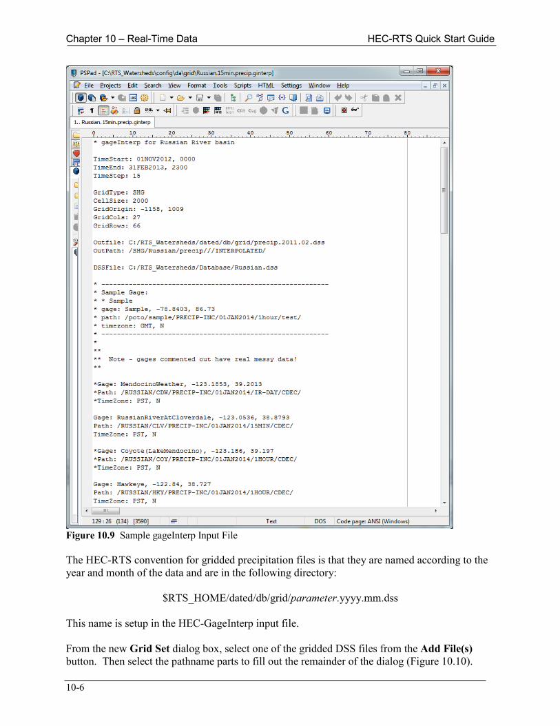
Chapter 10 – Real-Time Data HEC-RTS Quick Start Guide
10-6
Figure 10.9 Sample gageInterp Input File The HEC-RTS convention for gridded precipitation files is that they are named according to the year and month of the data and are in the following directory:
$RTS_HOME/dated/db/grid/parameter.yyyy.mm.dss This name is setup in the HEC-GageInterp input file. From the new Grid Set dialog box, select one of the gridded DSS files from the Add File(s) button. Then select the pathname parts to fill out the remainder of the dialog (Figure 10.10).
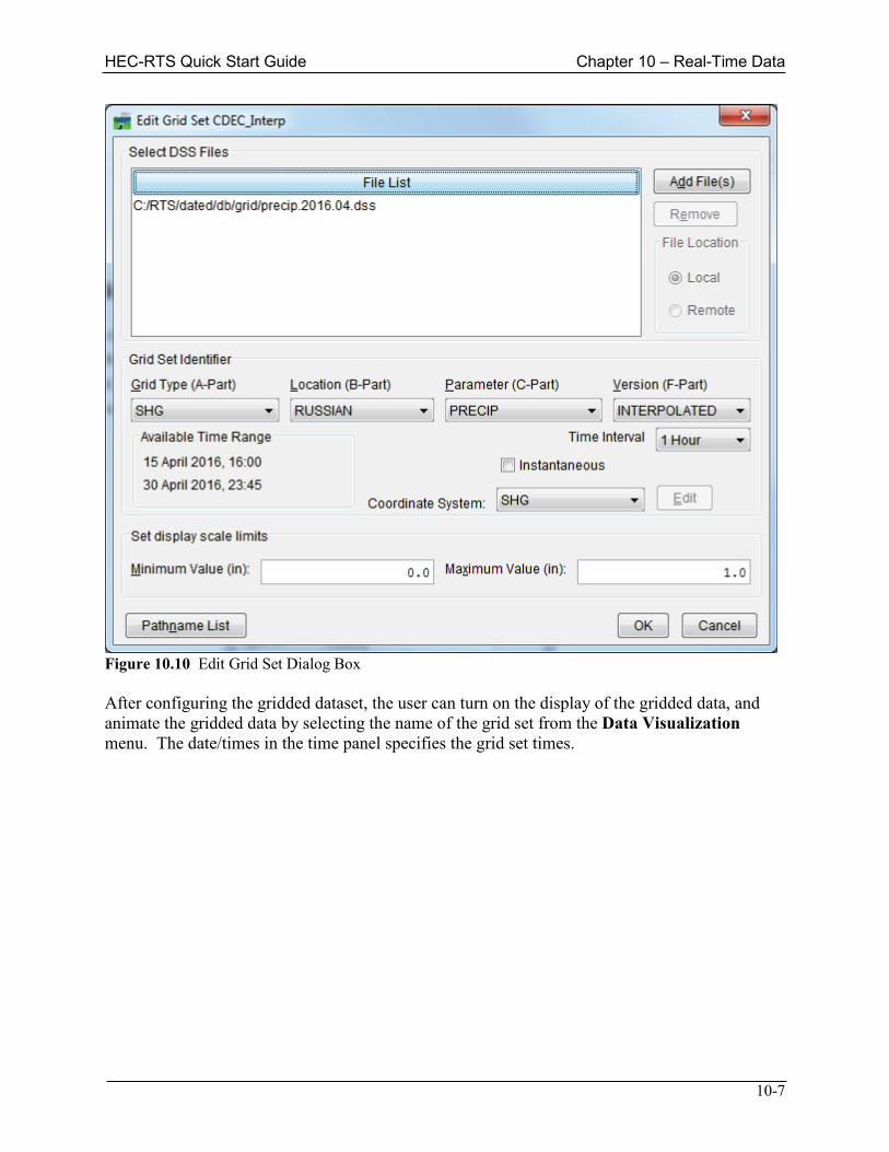
HEC-RTS Quick Start Guide Chapter 10 – Real-Time Data
10-7
Figure 10.10 Edit Grid Set Dialog Box After configuring the gridded dataset, the user can turn on the display of the gridded data, and animate the gridded data by selecting the name of the grid set from the Data Visualization menu. The date/times in the time panel specifies the grid set times.

Chapter 10 – Real-Time Data HEC-RTS Quick Start Guide
10-8


