RECENT METHODOLOGICAL AND COMPUTATIONAL ADVANCES IN STOCHASTIC POWER SYSTEM PLANNING Mario Pereira [email protected]with PSR researchers: Ricardo Perez, Camila Metello, Joaquim Garcia Pedro Henrique Melo and Lucas Okamura CMU EWO Seminar October 13, 2016
Transcript
RECENT METHODOLOGICAL ANDCOMPUTATIONAL ADVANCES IN STOCHASTIC
PSRProvider of analytical solutions and consulting services in electricity and natural gas since 1987
Our team has 54 experts (17 PhDs, 31 MSc) in engineering, optimization, energy systems, statistics, finance, regulation, IT and environment analysis
2
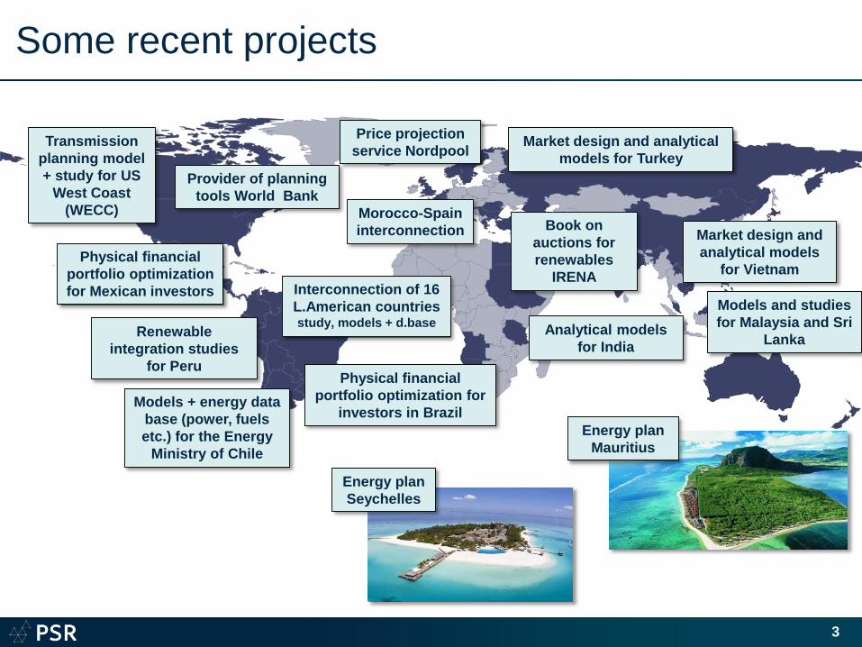
Some recent projects
3
Transmission planning model + study for US
West Coast (WECC)
Models and studies for Malaysia and Sri
Lanka
Price projection service Nordpool
Models + energy data base (power, fuels etc.) for the Energy
Ministry of Chile
Morocco-Spain interconnection
Interconnection of 16 L.American countries study, models + d.base
Market design and analytical models for Turkey
Physical financial portfolio optimization for Mexican investors
Provider of planning tools World Bank
Book on auctions for renewables
IRENA
Market design and analytical models
for Vietnam
Physical financial portfolio optimization for
investors in Brazil
Analytical models for India
Renewable integration studies
for Peru
Energy plan Seychelles
Energy plan Mauritius
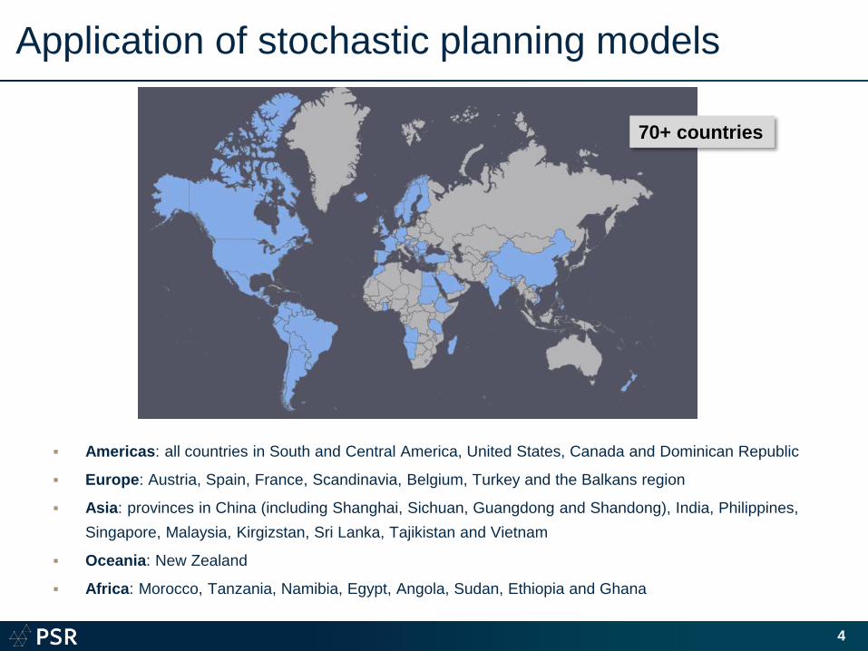
Application of stochastic planning models
Americas: all countries in South and Central America, United States, Canada and Dominican Republic
Europe: Austria, Spain, France, Scandinavia, Belgium, Turkey and the Balkans region
Asia: provinces in China (including Shanghai, Sichuan, Guangdong and Shandong), India, Philippines, Singapore, Malaysia, Kirgizstan, Sri Lanka, Tajikistan and Vietnam
Oceania: New Zealand
Africa: Morocco, Tanzania, Namibia, Egypt, Angola, Sudan, Ethiopia and Ghana
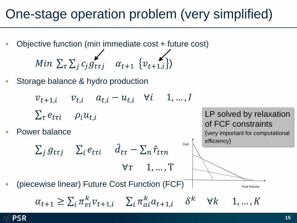
LP solved by relaxation of FCF constraints(very important for computational efficiency)
Cost
Final Volume
SDDP characteristics
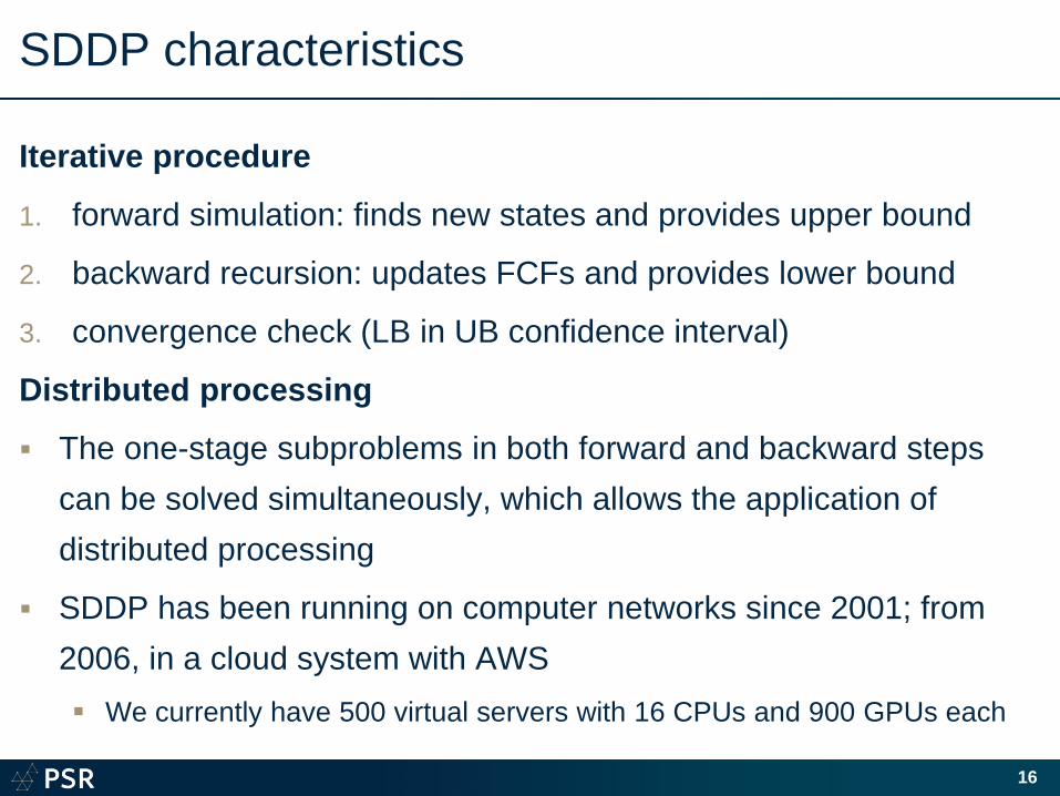
Iterative procedure
1. forward simulation: finds new states and provides upper bound
2. backward recursion: updates FCFs and provides lower bound
3. convergence check (LB in UB confidence interval)
Distributed processing
The one-stage subproblems in both forward and backward steps can be solved simultaneously, which allows the application of distributed processing
SDDP has been running on computer networks since 2001; from 2006, in a cloud system with AWS We currently have 500 virtual servers with 16 CPUs and 900 GPUs each
16
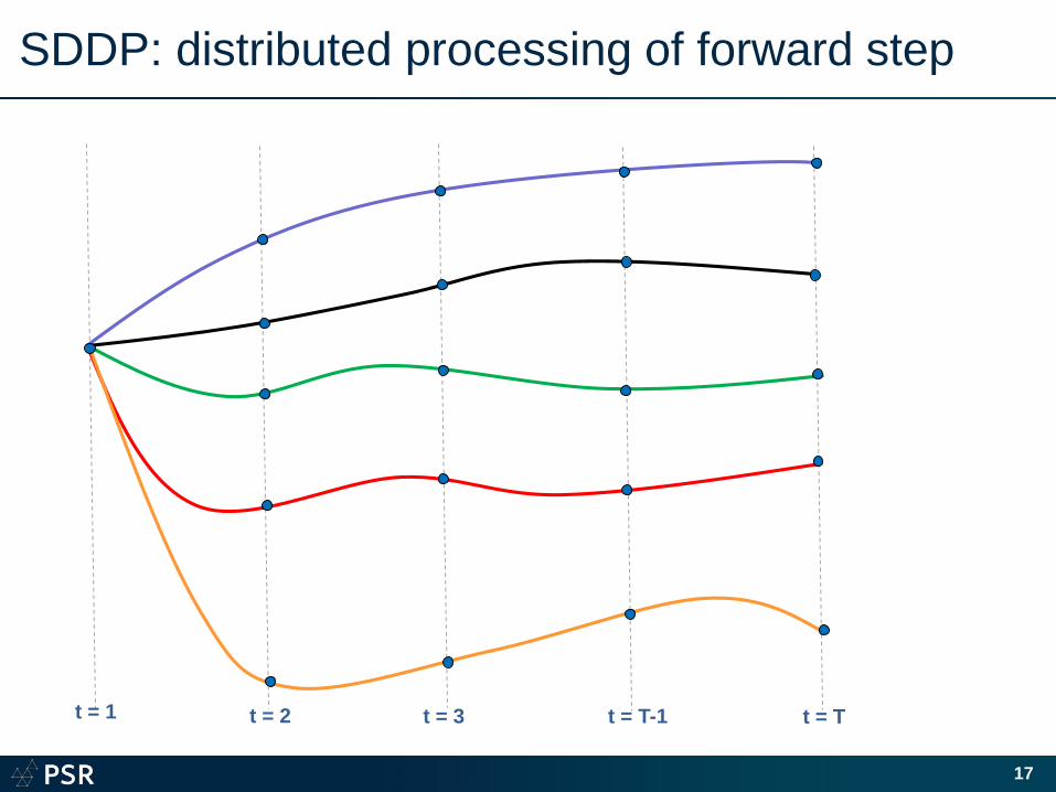
SDDP: distributed processing of forward step
17
t = 1 t = 2 t = 3 t = T-1 t = T
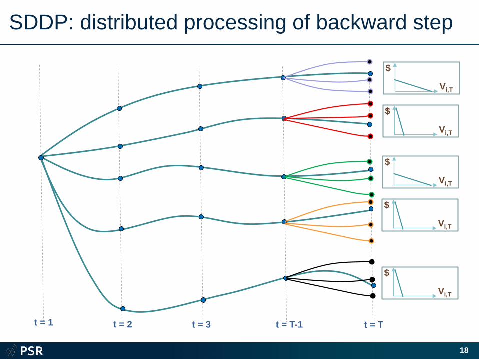
SDDP: distributed processing of backward step
18
t = 1 t = 2 t = 3 t = T-1 t = T
Vi,T
$
Vi,T
$
Vi,T
$
Vi,T
$
Vi,T
$
Example of SDDP run with distributed processing
Installed capacity: 125 GW
160 hydro plants (85 with storage), 140
thermal plants (gas, coal, oil and nuclear),
8 GW wind, 5 GW biomass, 1 GW solar
Transmission network: 5 thousand buses,
7 thousand circuits
State variables: 85 (storage) + 160 x 2 = 320 (AR-2 past inflows) = 405Monthly stages: 120 (10 years)Load blocks: 3
Forward scenarios: 1,200Backward branching: 30LP problems per stage/iteration: 36,000Number of SDDP iterations: 10Total execution time: 90 minutes25 servers with 16 processors each
19
Recent SDDP development: analytical ICF
► The very fast growth of renewables has raised concerns about operating difficulties when they are integrated to the grid For example, “wind spill” in the Pacific Northwest, need for higher reserve
margins due to the variability, hydro/wind/solar portfolio etc.
► The analysis of these issues requires hourly (or shorter) intervals in the intra-stage operation model ⇒ increase in computational effort
20
Constraints 3 Block problem Hourly problem
Water balance constraints 161 + 117,000 Load balance constraints 12 + 2,900 Maximum generation & turbining constraints 900 +219,000 Maximum & minimum volume constraints 322 +235,000 Total 1461 +573,000
0
10
20
30
40
50
60
70
80
90
100
0 100 200 300 400 500 600 700 800
Brazilian systemLP solution time x number of load blocks
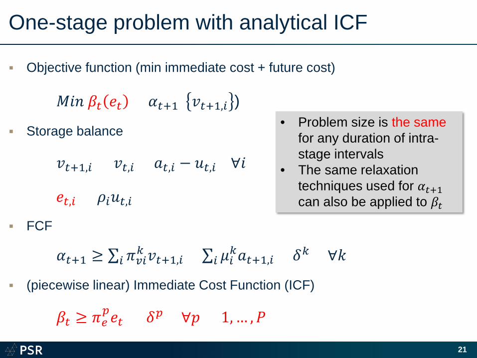
One-stage problem with analytical ICF
Objective function (min immediate cost + future cost)
• Problem size is the same for any duration of intra-stage intervals
• The same relaxation techniques used for 𝛼𝛼𝑡𝑡+1can also be applied to 𝛽𝛽𝑡𝑡
Pre-calculation of 𝛽𝛽𝑡𝑡 𝑒𝑒𝑡𝑡 : single area
► The analytical ICF can be seen as a multiscaling technique: theweekly (or monthly) operation problem represents explicitly thevariables with slower dynamics, in particular, the storage statevariables; the faster dynamics (hourly balance) are representedimplicitly in the ICF
► The idea is to pre-calculate all vertices (breakpoints) of thepiecewise function 𝛽𝛽𝑡𝑡 𝑒𝑒𝑡𝑡 and transform them into hyperplanes
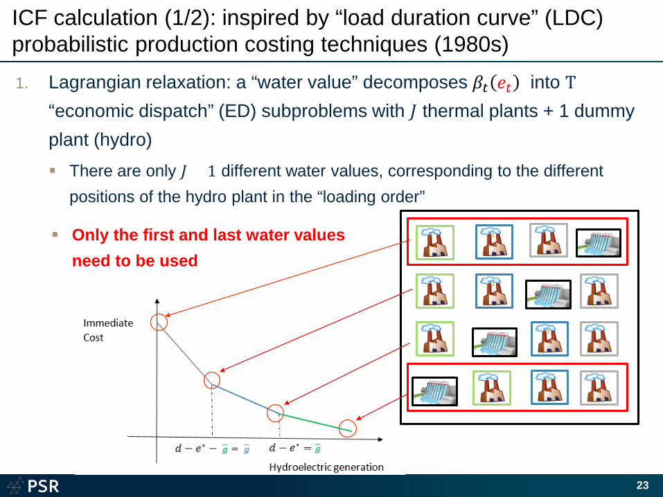
ICF calculation (1/2): inspired by “load duration curve” (LDC) probabilistic production costing techniques (1980s)1. Lagrangian relaxation: a “water value” decomposes 𝛽𝛽𝑡𝑡 𝑒𝑒𝑡𝑡 into Τ
“economic dispatch” (ED) subproblems with 𝐽𝐽 thermal plants + 1 dummy plant (hydro) There are only 𝐽𝐽 + 1 different water values, corresponding to the different
positions of the hydro plant in the “loading order”
23
Only the first and last water valuesneed to be used
Solution approach (2/2)
2. Each ED subproblem is further decomposed into 𝐽𝐽 + 1
generation adequacy subproblems, where we just
compare available capacity with (demand – renewables)
(arithmetic operation)
Expected thermal generation of plant 𝑗𝑗 (in the loading order) =
(EPNS without 𝑗𝑗) – (EPNS with 𝑗𝑗)
24
⇒ Computational effort is very small(and can be done in parallel)
► The multiarea generation adequacy is a max-flow problem
► Max flow – min cut ⇒ problem becomes max {2𝑀𝑀 linear segments}
Pre-calculation of 𝛽𝛽𝑡𝑡 𝑒𝑒𝑡𝑡 : 𝑀𝑀 areas
25
𝑆𝑆
1
𝑇𝑇
2
3
𝑔𝑔1
𝑔𝑔2
𝑔𝑔3
𝑓𝑓12
𝑓𝑓13 𝑓𝑓23
𝑑𝑑3
𝑑𝑑2
𝑑𝑑1
𝑀𝑀𝑎𝑎𝑀𝑀 𝛿𝛿 𝛿𝛿
𝑆𝑆
1
𝑇𝑇
2
3
𝑔𝑔1
𝑔𝑔2
𝑔𝑔3
𝑓𝑓12
𝑓𝑓13 𝑓𝑓23
𝑑𝑑3
𝑑𝑑2
𝑑𝑑1
𝑀𝑀𝑎𝑎𝑀𝑀 𝛿𝛿 𝛿𝛿
Cut 𝐴𝐴
Cut 𝐶𝐶
Cut 𝐵𝐵
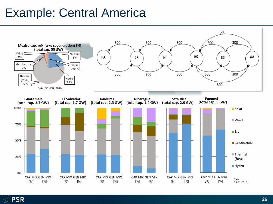
Example: Central America
26
Data: CRIE, 2015.
Data: UPME, 2015.Data: SENER, 2016.
4
SDDP execution time with/without analytical ICF
28
Current research
► Representation of storage (e.g. batteries) in the hourly
problem: the analytical approximation still applies, but the max
flow problem becomes larger due to time coupling; advanced
max flow techniques used in machine learning being tested
► New formulation that allows the representation of unit
commitment (per block of hours) and an (approximate)
transmission network
28
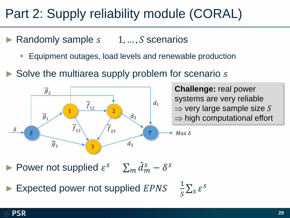
► Randomly sample 𝑠𝑠 = 1, … , 𝑆𝑆 scenarios
Equipment outages, load levels and renewable production
► Solve the multiarea supply problem for scenario 𝑠𝑠
► Power not supplied 𝜀𝜀𝑠𝑠 = ∑𝑚𝑚 �̂�𝑑𝑚𝑚𝑠𝑠 − 𝛿𝛿𝑠𝑠
► Expected power not supplied 𝐸𝐸𝑃𝑃𝐸𝐸𝑆𝑆 = 1𝑆𝑆∑𝑠𝑠 𝜀𝜀𝑠𝑠
𝑆𝑆
1
𝑇𝑇
2
3
𝑔𝑔1
𝑔𝑔2
𝑔𝑔3
𝑓𝑓12
𝑓𝑓13 𝑓𝑓23
𝑑𝑑3
𝑑𝑑2
𝑑𝑑1
𝑀𝑀𝑎𝑎𝑀𝑀 𝛿𝛿 𝛿𝛿
Part 2: Supply reliability module (CORAL)
29
Challenge: real power systems are very reliable ⇒ very large sample size 𝑆𝑆⇒ high computational effort
Recent advances: GPUs
► GPUs can provide a very large amount of numerical
processing capacity for a comparatively low price
► Limitation: GPUs are optimized for algebraic operations
𝐴𝐴𝑀𝑀𝑠𝑠 = 𝑏𝑏𝑠𝑠, 𝑠𝑠 = 1, … , 𝑆𝑆
► Max-flow min cut allows GPU application to multi-area
reliability
30
𝑆𝑆
1
𝑇𝑇
2
3
𝑔𝑔1
𝑔𝑔2
𝑔𝑔3
𝑓𝑓12
𝑓𝑓13 𝑓𝑓23
𝑑𝑑3
𝑑𝑑2
𝑑𝑑1
𝑀𝑀𝑎𝑎𝑀𝑀 𝛿𝛿 𝛿𝛿
Cut 𝐴𝐴
Cut 𝐶𝐶
Cut 𝐵𝐵
Example: same Central America system
► Notebook: I7 processor (2.4GHz) and a 384-core GPU
86 candidate projects per year (x 9 years) 27 thermal plants (natural gas, combined and open cycle)
8 hydro plants
7 renewable projects (4 wind farms and 3 solar)
44 transmission lines and transformers
Computational results
Number of Benders iterations (investment module): 55
Average number of SDDP iterations (stochastic scheduling for each candidate plan in the Benders scheme): 5 Forward step: 100 scenarios
Backward step: 30 scenarios (“branching”)
Total execution time: 4h 20m 2 servers x 16 processors = 32 CPUs
39
Bolivia integrated G&T planning (4/4)
40
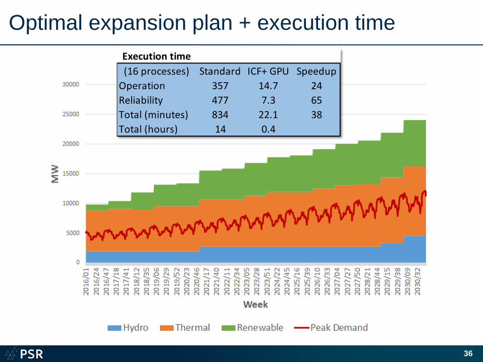
G&T Optimal Expansion Plan:
G: 9 TPPs, 7 HPPs, 3 Wind Farms
T: 12 Circuits (9 TLs and 3 Transf.)
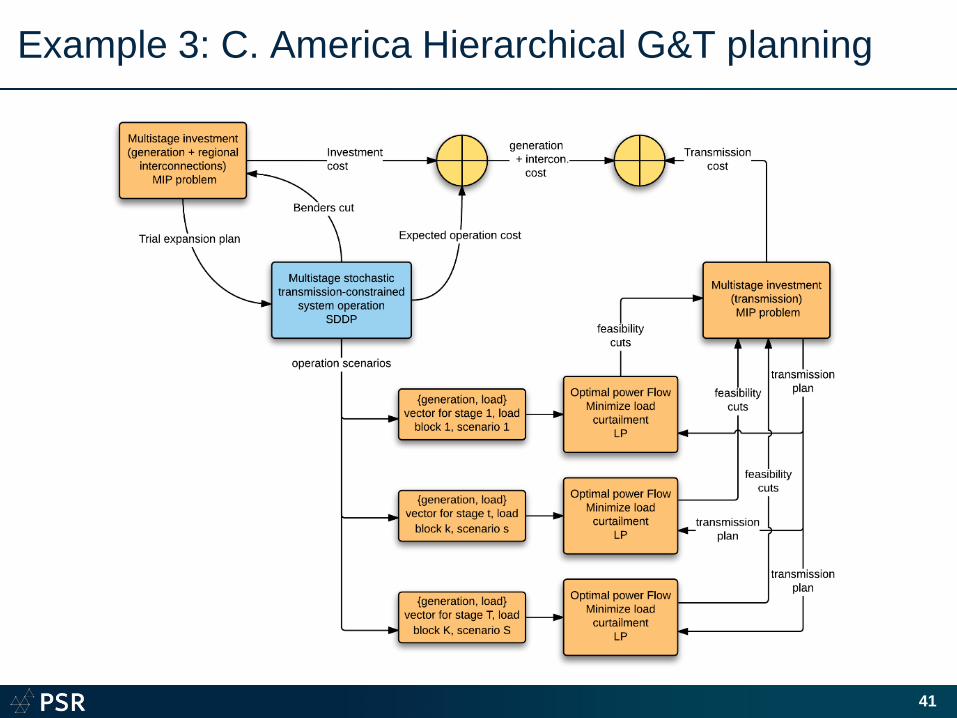
Example 3: C. America Hierarchical G&T planning
41
Hierarchical G&T Approach - Example: CA
42
MER transmission network visualization in PSR’s PowerView Tool
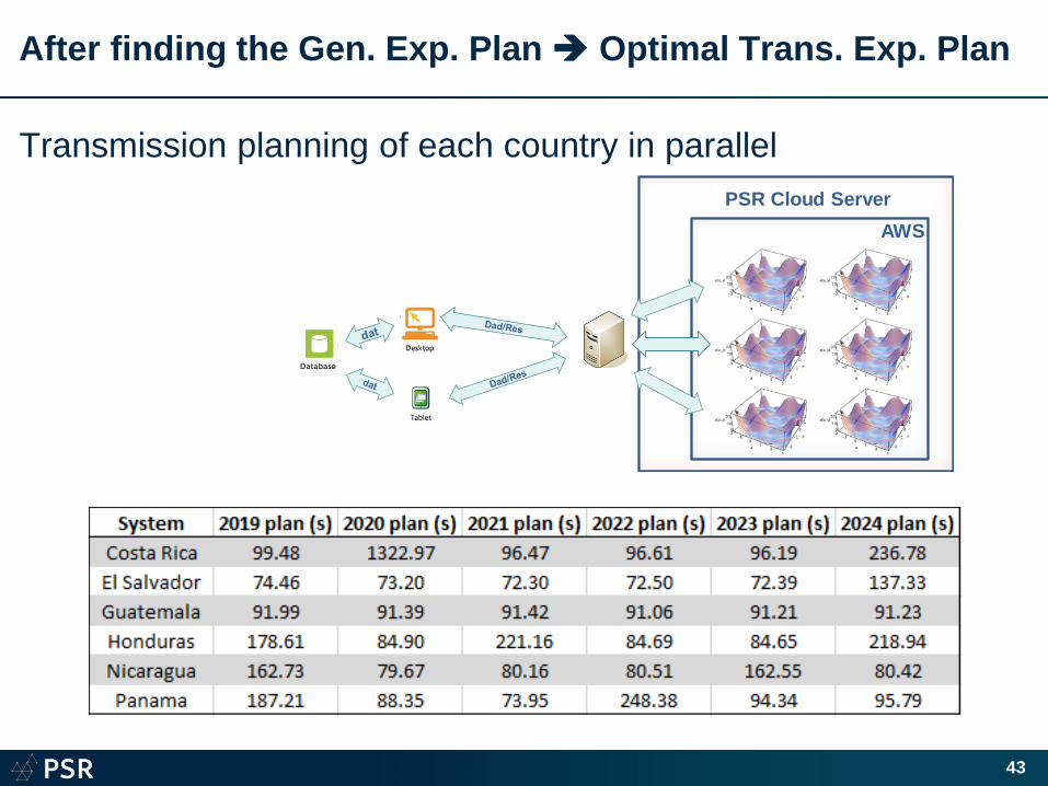
After finding the Gen. Exp. Plan Optimal Trans. Exp. Plan
43
Transmission planning of each country in parallelPSR Cloud Server
AWS
Conclusions
► Extensive experience with the application of stochastic scheduling and planning models to large-scale systems SDDP/SDP and Benders decomposition
Detailed modeling of generation, transmission, fuel storage and distribution, plus load response
► Multivariate AR models + Markov chains + scenarios can be used to represent uncertainties on inflows, renewable production, fuel costs, equipment availability and load
► The analytical ICF allows an efficient representation of multiple scale devices
► Parallel processing and, more recently, GPUs, are an essential component of the decomposition-based implementations