American Institute of Aeronautics and Astronautics1

Recent NASA Research on Aerodynamic Modeling of Post-Stall and Spin Dynamics of Large Transport Airplanes

Austin M. Murch1 and John V. Foster2

NASA Langley Research Center, Hampton, VA, 23681-2199

A simulation study was conducted to investigate aerodynamic modeling methods forprediction of post-stall flight dynamics of large transport airplanes. The research approachinvolved integrating dynamic wind tunnel data from rotary balance and forced oscillationtesting with static wind tunnel data to predict aerodynamic forces and moments duringhighly dynamic departure and spin motions. Several state-of-the-art aerodynamic modelingmethods were evaluated and predicted flight dynamics using these various approaches werecompared. Results showed the different modeling methods had varying effects on thepredicted flight dynamics and the differences were most significant during uncoordinatedmaneuvers. Preliminary wind tunnel validation data indicated the potential of the variousmethods for predicting steady spin motions.

Nomenclatureα = angle of attack, degrees

aveα = average value of αβ = angle of sideslip, degrees

aveβ = average value of β

bp = body-axis roll rate, degrees/second or radians/second

bq = body-axis pitch rate, degrees/second or radians/second

br = body-axis yaw rate, degrees/second or radians/secondΩ = total angular rate, degrees/second

xzΩ = projection of the total angular rate into the body-axis x-z plane, degrees/secondω = wind-axis (velocity-vector) roll rate, degrees/second or radians/second

aveω = average value of ωb = wingspan, feetL = length, feetc = mean aerodynamic chord, feetV = airspeed, feet/second

p = nondimensional body-axis roll rate ,2

bp bV

q = nondimensional body -axis pitch rate ,2

bq cV

r = nondimensional body -axis yaw rate ,2

br bV

ω = nondimensional wind-axis roll rate ,2

bV

ω

oscp = oscillatory component assigned to body-axis roll rate, degrees/second

1 Research Engineer, Flight Dynamics Branch, Mail Stop 308, AIAA Member.2 Senior Research Engineer, Flight Dynamics Branch, Mail Stop 308, AIAA Associate Fellow.

American Institute of Aeronautics and Astronautics2

oscq = oscillatory component assigned to body-axis pitch rate, degrees/second

oscr = oscillatory component assigned to body-axis yaw rate, degrees/second

oscΩ = total oscillatory angular rate component, degrees/second

ssω = steady-state component assigned to wind-axis roll rate, degrees/second

lC = aerodynamic rolling moment coefficient

mC = aerodynamic pitching moment coefficient

nC = aerodynamic yawing moment coefficient∆ = denotes increment

rδ = rudder deflection, positive trailing edge left, degrees

eδ = elevator deflection, positive trailing edge down, degrees

Raδ = right aileron deflection, positive trailing edge down, degrees

Laδ = left aileron deflection, positive trailing edge down, degreesCG = center of gravity, percent mean aerodynamic chordDIR = direct resolution blending method2D-KAL = 2D Kalviste blending methodHY-KAL = Hybrid Kalviste blending methodEXRR = Excess Roll Rate blending methodFO = forced oscillationRB = rotary balanceNASA = National Aeronautics and Space AdministrationLaRC = Langley Research Center

I. IntroductionS part of the NASA Aviation Safety Program, research has been conducted to develop aerodynamic modelingmethods for simulations that accurately predict the flight dynamics characteristics of large transport airplanes

in upset conditions1,2. The motivation for this research stems from the recognition that simulation is a vital tool foraddressing loss-of-control accidents, including applications to pilot training, accident reconstruction, and advancedcontrol system analysis. The ultimate goal of this effort is to contribute to the reduction of the fatality rate due toloss-of-control accidents.

An important part of aerodynamic modeling for loss-of-control scenarios involves prediction of stall, departureand incipient spin motions that have been observed during some accidents. Significant advances in aerodynamicmodeling of fighter configurations in post-stall and spin conditions have been achieved over the past severaldecades, but it is only recently that simulations of transport configurations in these flight regimes has gained interest.However, it has been recognized that flight validation of full-scale transport airplanes in post-stall regimes, incontrast to fighter configurations, is severely limited due to the unacceptable flight safety risks. As a result, the useof unmanned subscale flight vehicles has been proposed as an alternative for validation of simulations in high-riskconditions3.

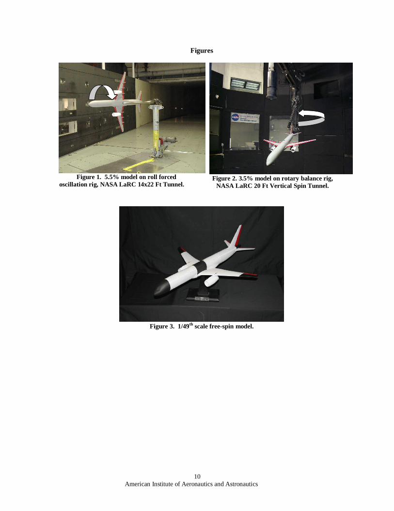
Current research is aimed at assessing and advancing state-of-the-art modeling methods for transportconfigurations and studying key flight dynamics characteristics of loss-of-control events. The research approachinvolves integrating dynamic wind tunnel data from rotary balance and forced oscillation testing with static windtunnel data to predict rigid-body aerodynamic forces and moments during highly dynamic post-stall/departuremotions. Previous research has been primarily aimed at methods to merge and blend data from dynamic testmethods in a way that emulates the aircraft motions4,5,6. Specifically, measurements from oscillatory motions (seeFig. 1) are combined with those from steady-state rotary motions (see Fig. 2) with the goal of predicting a range ofmotions typical of loss-of-control events. Results from previous research have indicated the need for advanced windtunnel test rigs (e.g. combined motion rigs) that more closely replicate real aircraft motions and have highlighted theneed for data reduction methods that better characterize and identify highly non-linear and time-dependentaerodynamic properties that are typical of separated flows.

This paper shows results of applying several state-of-the-art aerodynamic modeling methods using dynamicwind tunnel data, for the purpose of predicting post-stall flight motions, along with comparisons of predicted flightdynamics using these various approaches. Results from a preliminary free-spin test of a subscale transport model(see Fig. 3) will be compared to simulation results as an initial validation of the modeling methods. Finally,

A

American Institute of Aeronautics and Astronautics3

recommendations regarding wind tunnel test methods, aerodynamic modeling approaches, and validationrequirements will be discussed.

II. ApproachThe approach to this research was to apply state-of-the-art aerodynamic modeling methods for post-stall and spin

motions to a transport configuration. The objective was to identify advantages, disadvantages, and/or limitations ofthese methods and to recommend future research needed to improve prediction of post-stall and spin flightdynamics.

A. BackgroundThe approach to aerodynamic modeling typically involves summation of static effects (e.g. angle of attack,

control position) with dynamic effects (e.g. angular rate), the latter often referred to as rate damping effects. Thetypical practice used today for large transport simulators is that static effects are normally based on wind tunnelmeasurements but prediction of the dynamic effects are usually accomplished using empirical methods7 or fromflight test data using small-amplitude dynamic maneuvers. These simulation models of large transport flightbehavior are normally not designed for upset conditions and therefore are limited to the normal flight envelopebelow stall angles of attack. Recent analysis of loss-of-control accidents8 revealed that the normal flight envelopewas often exceeded during loss-of-control accidents, and angles of attack well beyond stall were observed. Furthersimulation studies7 have also shown that accurate modeling of angular rate effects on large transports had asignificant effect on the predicted aircraft behavior, which exposed the need for more detailed investigation of thepost-stall dynamic behavior.

Aerodynamic modeling of highly dynamic maneuvers such as post-stall gyrations, spins, and other out-of-controlmotions is not a new problem. In the past thirty years, these motions have been modeled for numerous fighteraircraft configurations5,6,9,10,11. In addition, stall/spin accidents led to modeling research of general aviation aircraftin the 1980’s, including studies by NASA12. In both cases, modeling the angular rate effects relied on two existingexperimental test methods; oscillatory motion rigs (i.e. forced oscillation) and steady motion rigs (i.e. rotarybalance). However, out-of-control motions often involve a combination of large amplitude, uncoordinated (i.e., theangular rate vector is not closely aligned with the velocity vector), and coupled motions which are difficult toreplicate with existing wind tunnel motion rigs. As a result, previous research focused on methods to blendoscillatory and steady rate effects and on the development of new motion rigs designed to more closely simulate realflight motions.

One approach to modeling dynamic effects is to combine the forced oscillation and rotary balance data setsbased on the characteristics of aircraft motion. The underlying assumption in this approach is that data from twofundamentally different dynamic wind tunnel test motions can be combined vectorially to approximate arbitrarydynamic motion of aircraft. While this approach presents many challenges in terms of modeling and similituderequirements, it has been used successfully and is the most commonly used approach to date. Several differentblending methods using this vectorial technique have been used effectively on fighter aircraft in the past. However,application of these methods to large transport configurations has been limited and is a motivating factor for thisresearch.

Although experience with out-of-control flight motions of transport airplanes is very limited, recent research hasshown significant differences in dynamic wind tunnel test results between fighter and transport configurations13. Asshown in Table I, comparison of flight data from loss-of-control motions of fighter aircraft14 and commercialtransports7 indicate both configurations can reach high post-stall wind incidence angles and similar nondimensionalrates during loss-of-control motions. However, in general, transport configurations are not expected to achieve ashigh wind incidence angles as fighters. A goal of this research is to identify the applicability of current blendingmethods to transport configurations and the following section provides a description of the blending methods used.

Table I. Comparison of Fighter and Commercial Aircraft Loss-of-Control Motions

Configuration maxα maxβ maxp maxq maxr

Fighter14 70° 45° 0.129 0.0062 0.043Transport7 47° 20° 0.126 0.0045 0.047

American Institute of Aeronautics and Astronautics4

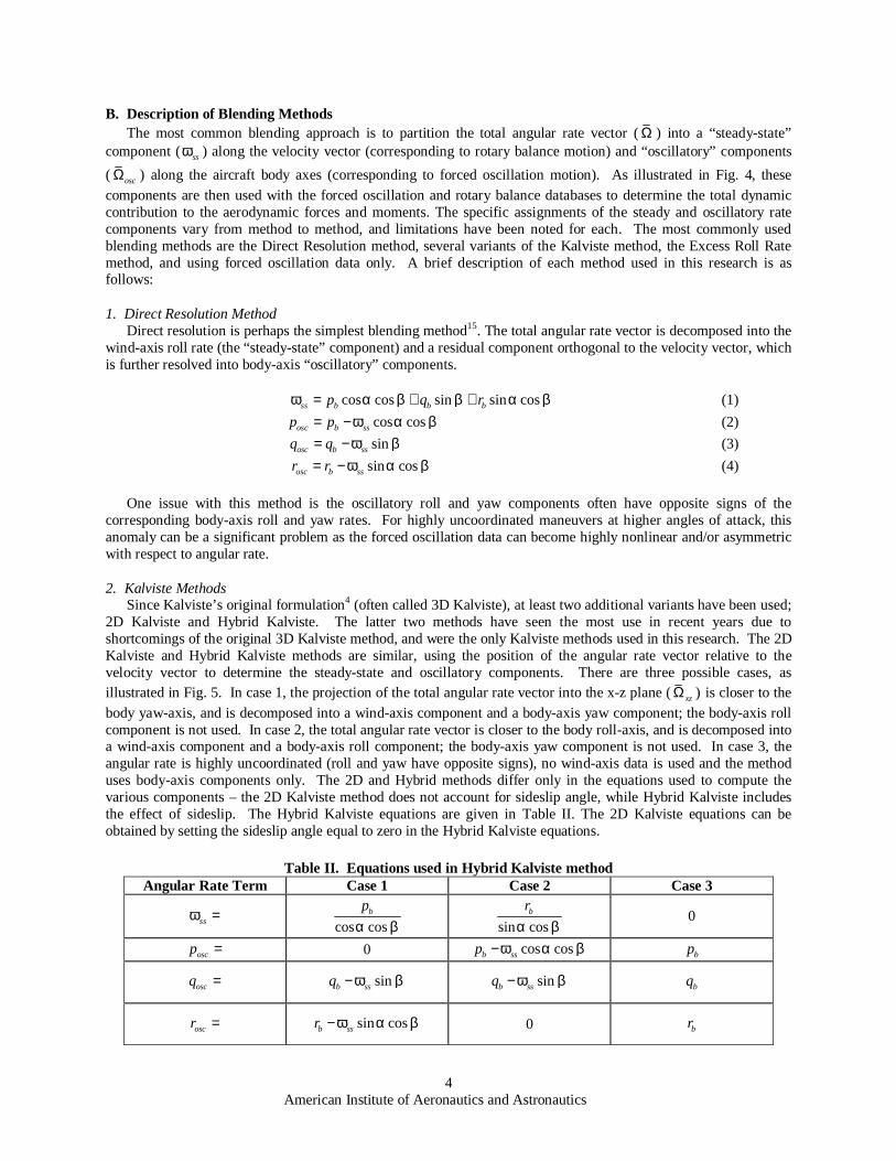
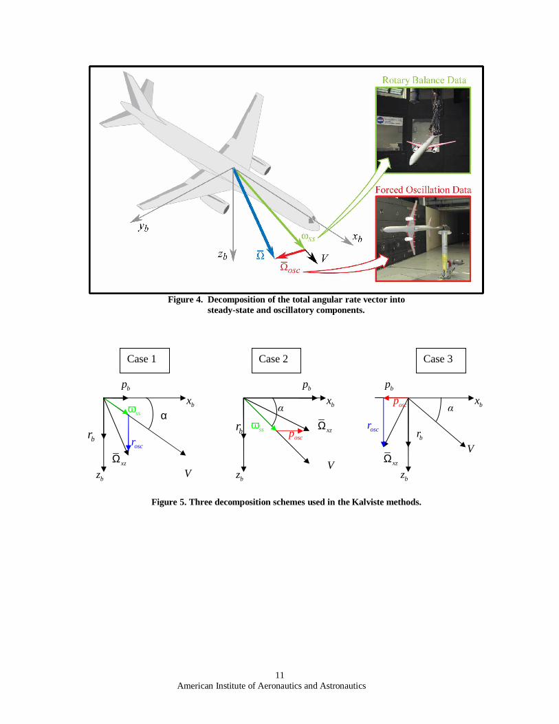
B. Description of Blending MethodsThe most common blending approach is to partition the total angular rate vector ( Ω ) into a “steady-state”

component ( ssω ) along the velocity vector (corresponding to rotary balance motion) and “oscillatory” components( oscΩ ) along the aircraft body axes (corresponding to forced oscillation motion). As illustrated in Fig. 4, thesecomponents are then used with the forced oscillation and rotary balance databases to determine the total dynamiccontribution to the aerodynamic forces and moments. The specific assignments of the steady and oscillatory ratecomponents vary from method to method, and limitations have been noted for each. The most commonly usedblending methods are the Direct Resolution method, several variants of the Kalviste method, the Excess Roll Ratemethod, and using forced oscillation data only. A brief description of each method used in this research is asfollows:

1. Direct Resolution MethodDirect resolution is perhaps the simplest blending method15. The total angular rate vector is decomposed into the

wind-axis roll rate (the “steady-state” component) and a residual component orthogonal to the velocity vector, whichis further resolved into body-axis “oscillatory” components.

cos cos sin sin cosss b b bp q rω α β β α β= + + (1)cos cososc b ssp p ω α β= − (2)sinosc b ssq q ω β= − (3)

sin cososc b ssr r ω α β= − (4)

One issue with this method is the oscillatory roll and yaw components often have opposite signs of thecorresponding body-axis roll and yaw rates. For highly uncoordinated maneuvers at higher angles of attack, thisanomaly can be a significant problem as the forced oscillation data can become highly nonlinear and/or asymmetricwith respect to angular rate.

2. Kalviste MethodsSince Kalviste’s original formulation4 (often called 3D Kalviste), at least two additional variants have been used;

2D Kalviste and Hybrid Kalviste. The latter two methods have seen the most use in recent years due toshortcomings of the original 3D Kalviste method, and were the only Kalviste methods used in this research. The 2DKalviste and Hybrid Kalviste methods are similar, using the position of the angular rate vector relative to thevelocity vector to determine the steady-state and oscillatory components. There are three possible cases, asillustrated in Fig. 5. In case 1, the projection of the total angular rate vector into the x-z plane ( xzΩ ) is closer to thebody yaw-axis, and is decomposed into a wind-axis component and a body-axis yaw component; the body-axis rollcomponent is not used. In case 2, the total angular rate vector is closer to the body roll-axis, and is decomposed intoa wind-axis component and a body-axis roll component; the body-axis yaw component is not used. In case 3, theangular rate is highly uncoordinated (roll and yaw have opposite signs), no wind-axis data is used and the methoduses body-axis components only. The 2D and Hybrid methods differ only in the equations used to compute thevarious components – the 2D Kalviste method does not account for sideslip angle, while Hybrid Kalviste includesthe effect of sideslip. The Hybrid Kalviste equations are given in Table II. The 2D Kalviste equations can beobtained by setting the sideslip angle equal to zero in the Hybrid Kalviste equations.

Table II. Equations used in Hybrid Kalviste methodAngular Rate Term Case 1 Case 2 Case 3

ssω =cos cos

bpα β sin cos

brα β

0

oscp = 0 cos cosb ssp ω α β− bp

oscq = sinb ssq ω β− sinb ssq ω β− bq

oscr = sin cosb ssr ω α β− 0 br

American Institute of Aeronautics and Astronautics5

Previous research efforts found the Kalviste methods to be sensitive to slightly uncoordinated maneuvers at veryhigh angles of attack, which can cause the method to abruptly switch to using forced oscillation data only6. Due tothe lower magnitude of wind angles experienced with transports, this sensitivity was not found in this research.

3. Excess Roll Rate MethodThe Excess Roll Rate method6 does not use a body-axis yaw component, and it uses the same equations as Case

2 of the Hybrid Kalviste method. This approach was intended to model roll rate-dominated motions and avoidscomplexities associated with using yaw forced oscillation data. One significant drawback of this method is thepresence of a singularity at 0α = °, which necessitates a different approach at low angles of attack. For thisresearch, Hybrid Kalviste was used if the angle of attack was less than 15°.

4. Forced Oscillation MethodPrevious research on blending methods found that using forced oscillation data alone (i.e., Case 3 of the Hybrid

Kalviste method) was not adequate to model highly dynamic post-stall motions6,10. For completeness, this methodwas studied and compared to the other blending methods. Results from the forced oscillation studies are not shownherein but are briefly discussed. One problem with this approach is that the angular rates attained in maneuvers suchas spins can exceed the limits of the forced oscillation database, invalidating the simulations results and possiblycausing the simulation to diverge.

C. Research MethodologyTwo approaches were used to analyze the various blending methods. The first approach focused on the

differences between the blending methods and examined how each method decomposed the angular rates for anoscillatory spin motion. The steady-state and oscillatory rate components from each method were compared, as wellas the aerodynamic coefficient increments produced from the aerodynamic model. The second approach was toexamine the effect of the blending method on post-stall and spin dynamics by implementing each method in a real-time MATLAB/Simulink-based simulation of a 5.5% dynamically-scaled commercial transport model16 (see Fig. 6).The simulation utilizes an extensive static wind tunnel-derived database developed as part of previous aerodynamicmodeling studies1. Databases from the aforementioned dynamic (forced oscillation and rotary balance) wind tunneltests were included in the simulations. The rotary balance database modeled effects of the six degree-of-freedomaerodynamic coefficients and was created as nonlinear look-up tables that are functions of angle of attack, sideslipangle, and nondimensional angular rate. The forced oscillation database was created as nonlinear look up tables thatare functions of angle of attack and nondimensional body-axis rate. Effects of nondimensional roll and yaw ratewere modeled for the aerodynamic side force, rolling moment, and yawing moment coefficients. Effects ofnondimensional pitch rate were modeled for the aerodynamic axial force, normal force, and pitching momentcoefficients.

To analyze the effect of the blending methods on post-stall and spin dynamics, an extensive simulator test usingnumerous spin entry techniques was conducted. Using identical initial conditions and control inputs with eachblending method, comparison of simulator time histories and key characteristics of the resulting motions providedinsight into the effect of each blending method on the overall aircraft motion. Although the potential for acommercial transport to enter a fully developed spin is small, analysis of the incipient and fully-developed spinprovided a good starting point because of the number of analysis tools available and extensive prior research.

Definitive conclusions as to which blending method, if any, provides the most accurate prediction of post-stalland spin dynamics require validation data. Validation of the modeling and blending methods is a difficult problem,given the unacceptable safety risks involved with operating commercial transports in the post-stall regime. For thepurposes of this research, preliminary free-spin test results of a subscale model were used as an initial assessment ofthe blending methods.

III. Results and Analysis

A. Blending Method ComparisonThe first task for this research focused on the differences between the blending methods and examined how each

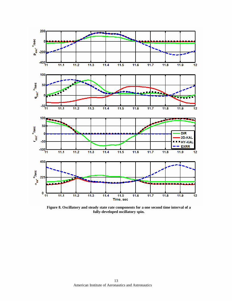
method decomposed an oscillatory spin motion. Figure 7 depicts a sample time history of angle of attack, sideslipangle, and body axis angular rates for an upright, moderately steep, oscillatory, right-hand spin that would beexpected for a 5.5% scale transport aircraft based on simulation results. Figure 8 illustrates how each blending

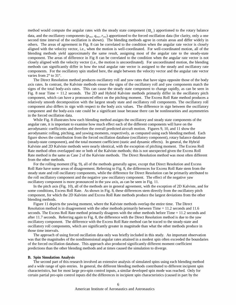
American Institute of Aeronautics and Astronautics6

method would compute the angular rates with the steady state component ( ssω ) apportioned to the rotary balancedata, and the oscillatory components (posc, qosc, rosc) apportioned to the forced oscillation data (for clarity, only a onesecond time interval of the oscillation is shown). The blending methods agree in certain areas and differ widely inothers. The areas of agreement in Fig. 8 can be correlated to the condition when the angular rate vector is closelyaligned with the velocity vector, i.e., when the motion is well-coordinated. For well-coordinated motion, all of theblending methods yield approximately the same result, assigning most of the angular rate to the steady-statecomponent. The areas of difference in Fig 8 can be correlated to the condition when the angular rate vector is notclosely aligned with the velocity vector (i.e., the motion is uncoordinated). For uncoordinated motion, the blendingmethods can significantly differ in how the total angular rate vector is assigned to the steady and oscillatory ratecomponents. For the oscillatory spin studied here, the angle between the velocity vector and the angular rate vectorvaries from 2° to 31°.

The Direct Resolution method produces oscillatory roll and yaw rates that have signs opposite those of the bodyaxis rates. In contrast, the Kalviste methods ensure the signs of the oscillatory roll and yaw components match thesigns of the total body-axis rates. This can cause the steady state component to change rapidly, as can be seen inFig. 8 near Time = 11.2 seconds. The 2D and Hybrid Kalviste methods primarily differ in the oscillatory pitchcomponent, which can have a pronounced effect on the pitching moment. The Excess Roll Rate method produces arelatively smooth decomposition with the largest steady state and oscillatory roll components. The oscillatory rollcomponent also differs in sign with respect to the body axis values. The difference in sign between the oscillatorycomponent and the body-axis rate could be a significant issue because there can be nonlinearities and asymmetriesin the forced oscillation data.

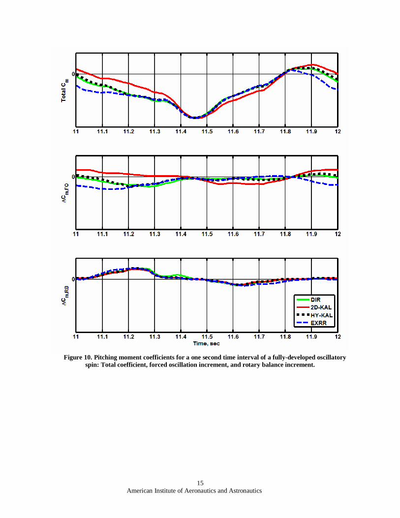
While Fig. 8 illustrates how each blending method assigns the oscillatory and steady state components of theangular rate, it is important to examine how much effect each of the different components will have on theaerodynamic coefficients and therefore the overall predicted aircraft motion. Figures 9, 10, and 11 show theaerodynamic rolling, pitching, and yawing moments, respectively, as computed using each blending method. Eachfigure shows the contribution from the forced oscillation database (oscillatory component), rotary balance database(steady-state component), and the total moment coefficient (static and dynamic effects). In general, the HybridKalviste and 2D Kalviste methods were nearly identical, with the exception of pitching moment. The Excess RollRate method often overlapped one or both of the Kalviste methods; this is not unexpected given the Excess RollRate method is the same as Case 2 of the Kalviste methods. The Direct Resolution method was most often differentfrom the other methods.

For the rolling moment (Fig. 9), all of the methods generally agree, except that Direct Resolution and ExcessRoll Rate have some areas of disagreement. Referring to Fig. 8, the differences for Excess Roll Rate stem from thesteady state and roll oscillatory components, while the difference for Direct Resolution can be primarily attributed tothe roll oscillatory component and the negative yaw oscillatory component. The effect of the negative yawoscillatory component is more pronounced in the yaw axis, as can be seen in Fig. 11.

In the pitch axis (Fig. 10), all of the methods are in general agreement, with the exception of 2D Kalviste, and forsome conditions, Excess Roll Rate. As shown in Fig. 8, these differences stem directly from the oscillatory pitchcomponent, for which the 2D Kalviste and Excess Roll Rate methods produce the largest deviations from the otherblending methods.

Figure 11 depicts the yawing moment, where the Kalviste methods overlap the entire time. The DirectResolution method is in disagreement with the other methods primarily between Time = 11.2 seconds and 11.6seconds. The Excess Roll Rate method primarily disagrees with the other methods before Time = 11.2 seconds andafter 11.7 seconds. Referring again to Fig. 8, the difference with the Direct Resolution method is due to the yawoscillatory component. The difference with the Excess Roll Rate method can be traced to the steady-state andoscillatory roll components, which are significantly greater in magnitude than what the other methods produce inthose time intervals.

The approach of using forced oscillation data only was briefly included in this study. An important observationwas that the magnitudes of the nondimensional angular rates attained in a modest spin often exceeded the boundariesof the forced oscillation database. This approach also produced significantly different moment coefficientpredictions than the other blending methods and at times caused the simulation to diverge.

B. Spin Simulation AnalysisThe second part of this research involved an extensive analysis of simulated spins using each blending method

and a wide range of spin entries. In general, the different blending methods contributed to different incipient spincharacteristics, but for most large pro-spin control inputs, a similar developed spin mode was reached. Only forcertain partial pro-spin control inputs did the differences in incipient spin characteristics (caused in part by the

American Institute of Aeronautics and Astronautics7

blending method used) lead to a difference in the developed spin mode. This result can be explained by examiningthe situations where the blending methods have the greatest effect on the overall motion. Care must be taken wheninterpreting this result, since the blending methods, static and dynamic aerodynamic effects, and control effects areall a function of the wind incidence angles.

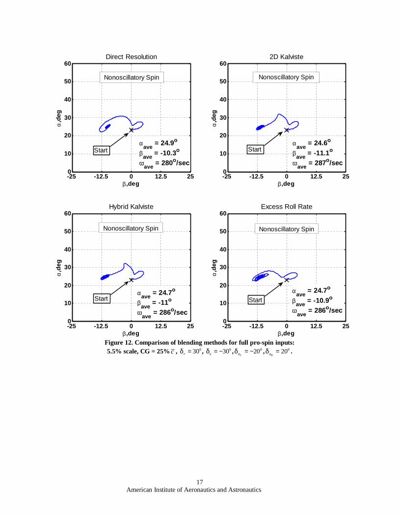
For well-coordinated maneuvers (e.g. nonoscillatory spins and velocity-vector rolls), the angular rate vector isclosely aligned with the relative wind vector. This type of motion is well replicated by rotary balance motion and allof the blending methods studied will give nearly the same decomposition and attribute the majority of the angularrate to the steady state rate component. For this reason, very little difference can be discerned in simulation resultsof well-coordinated maneuvers using different blending methods. Figure 12 shows angle of attack plotted versussideslip angle for an incipient and fully-developed nonoscillatory spin using each blending method. Note thedifference in the incipient spin trajectories (which begin at 23 , 0α β= =o o ) between blending methods; this iswhere the motion is uncoordinated. As the spin develops, the motion becomes more coordinated and each blendingmethod gives similar results, so few differences can be discerned between the steady spins predicted by eachmethod.

For uncoordinated maneuvers (e.g. incipient spins, oscillatory spins, and post-stall gyrations), the angular ratevector is not closely aligned with the relative wind vector. In this case each blending methods produces differentdynamic aerodynamic contributions. The different dynamic effects produced by the blending methods are largeenough to cause different incipient spin characteristics and different trajectories throughout the fully-developed spinphase, but typically not enough to affect the general characteristics of the spin (e.g. change an oscillatory spin into anonoscillatory spin).

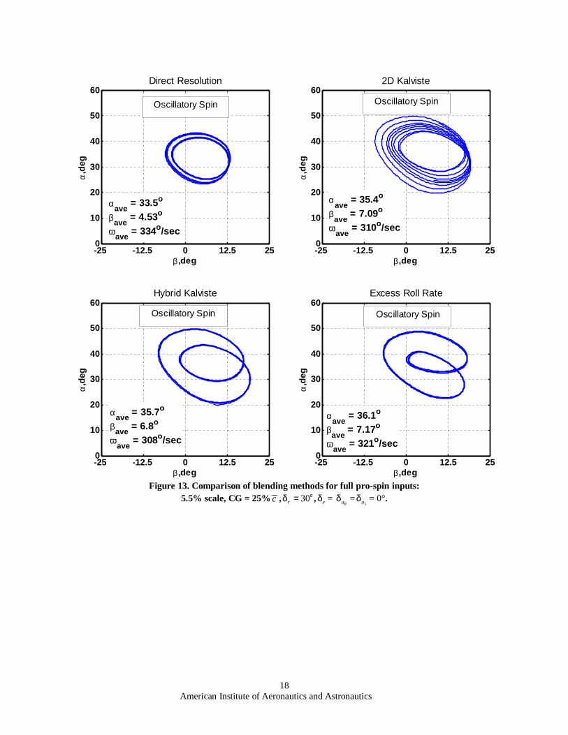
Figure 13 shows the angle of attack plotted versus sideslip angle for a fully-developed oscillatory spin using eachblending method. The general characteristics of all of these spins are the same; upright, moderately steep,oscillatory, and high spin rates. Referring to the annotations on Fig. 13, note the average values for angle of attack,sideslip angle, and spin rate for all the spins are nearly the same. However the characteristics of the oscillations arevery different when viewed in the α β− plane. The Direct Resolution method produces the least oscillatory spin,with the fastest spin rate and lowest average angle of attack. The 2D Kalviste method produced an oscillation ofvarying amplitude, while the Hybrid Kalviste and Excess Roll Rate methods had similar oscillation patterns. Notethat both Kalviste methods and the Excess Roll Rate method had very similar average values of angle of attack,sideslip angle, and spin rate despite the differences in oscillation characteristics. While the blending methodsexhibit the greatest dissimilarities during uncoordinated motion, the differences in trajectories noted here cannot becompletely attributed to differences in the blending methods, since the static aerodynamics and control effects arealso a function of the wind incidence angles. However, since the dynamic aerodynamic effects are significant for adeveloped spin, the dissimilarities in the blending methods will likely have a considerable effect on the oscillationcharacteristics.

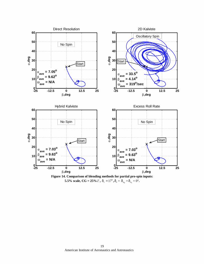
In certain spin entries with partial pro-spin control inputs, the choice of blending method had a significant effecton the general characteristic of the spin. In these cases, the control effects are not as dominant in the overallaerodynamics, allowing the dynamic aerodynamic effects to play a more significant role in the incipient phase of thespin and which developed spin mode, if any, will be reached. For example, as depicted in Fig. 14, a spin entry with

rδ = 17° eδ =Raδ =

Laδ = 0° did not produce a spin using the Direct Resolution, Hybrid Kalviste, or Excess Roll Ratemethods, but produced an oscillatory spin using the 2D Kalviste method. This is one example of how dissimilaritiesin the dynamic aerodynamic effects produced by the blending methods can have a dramatic effect on the predictionof the developed motion.

In summary, this analysis indicated the choice of blending method will have the largest effect duringuncoordinated maneuvers such as post-stall gyrations, incipient spins, and fully-developed oscillatory spins.Whether the impact of the blending method will be enough to radically affect the developed motion depends largelyupon the control inputs used. This study showed that for less than full pro-spin control inputs, the dynamicaerodynamic effects can play a significant role in determining the developed motion, so that the choice of blendingmethod becomes more important for prediction of post-stall and spin dynamics. Since loss-of-control motions rarelyinvolve full, sustained pro-spin controls, the blending method used will likely be an important factor in accuratelypredicting these types of motion.

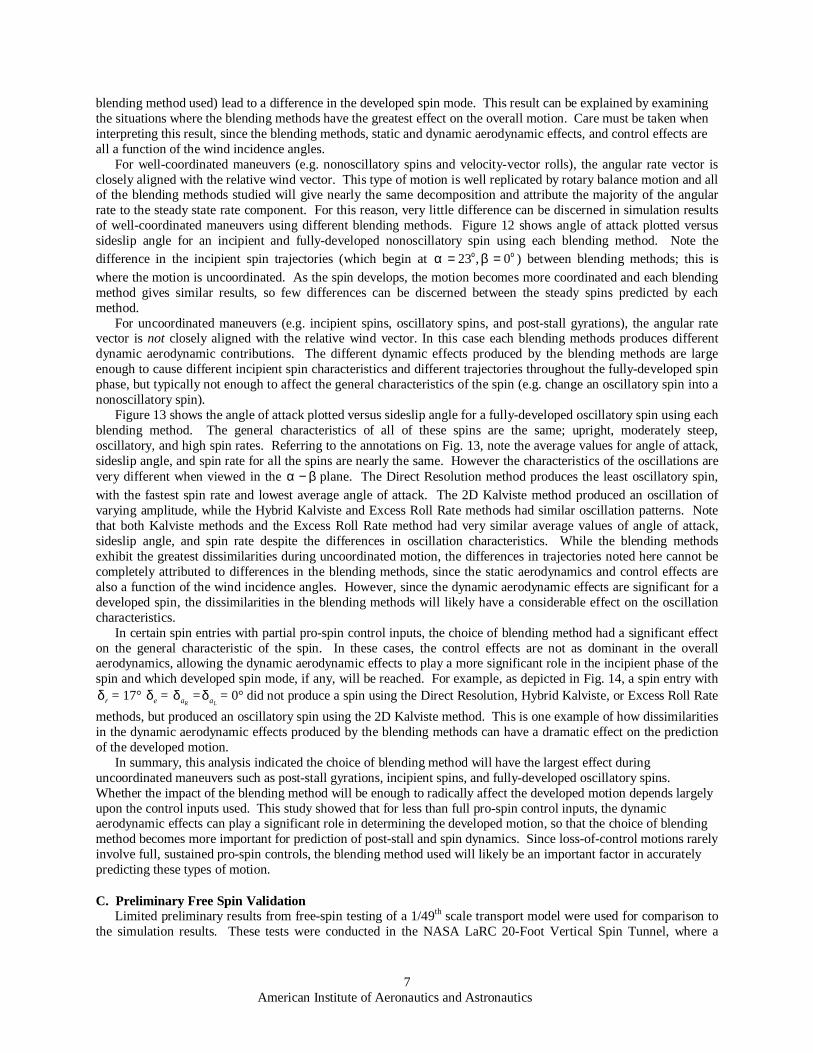
C. Preliminary Free Spin ValidationLimited preliminary results from free-spin testing of a 1/49th scale transport model were used for comparison to

the simulation results. These tests were conducted in the NASA LaRC 20-Foot Vertical Spin Tunnel, where a

American Institute of Aeronautics and Astronautics8

sustained, upright oscillatory spin was demonstrated using rδ = 30° eδ =Raδ =

Laδ = 0° and CG = 15.2% c .Simulations using the same scale, inertia loadings, control inputs, and similar initial conditions as the free-spin testalso produced an upright oscillatory spin with similar nondimensional spin rate. Estimated nondimensional spin ratewas the only data available from the free-spin test, and Fig. 15 shows this data compared to simulations using eachblending method. While not a rigorous or complete validation, this preliminary result indicates that the blendingmethods evaluated give reasonable results for a transport aircraft configuration.

D. Future PlansFuture research will focus on validating the modeling methods. This activity will allow recommendations to be

made regarding use of the four blending methods studied for modeling departures, incipient and fully-developedspin dynamics of transport aircraft. First, free-spin testing in the 20-Foot Vertical Spin Tunnel will be conducted toanalyze a range of control inputs and spin conditions. Secondly, flight testing with unmanned subscale models isplanned in order to validate post-stall and incipient spin phases. The validation activities may also lead todevelopment of new modeling approaches and application to full-scale simulations.

IV. ConclusionsBased upon the simulation study and limited free-spin test results, the following conclusions can be made:

1. Simulation results using each blending method exhibited different incipient spin characteristics, but for mostlarge pro-spin control inputs a similar fully-developed spin mode was reached. Differences in the oscillationcharacteristics of oscillatory spin modes were noted for each blending method used. Only for certain partial pro-spin control inputs did the blending method lead to a difference in the developed spin mode obtained.2. The largest differences between the blending methods occurred during uncoordinated maneuvers such as post-stall gyrations, incipient spins, and oscillatory spins, and especially in cases with less than full control deflections.3. The simulation study indicated that using forced oscillation data alone did not agree with any of the methodsusing rotary balance data. In addition, angular rates predicted by using forced oscillation data alone often exceededthe database limits.4. All blending methods evaluated in this study predicted average spin rates that were in general agreement withpreliminary free-spin test results.5. Validation data is needed to determine the blending method that will produce the most accurate departure andspin predictions for transport aircraft configurations.

References1Shah, G.H., Cunningham, K. Foster, J.V., Fremaux, C. M. Stewart, E.C., Wilborn, J. E., Gato, W., and Pratt, D. W., “Wind-Tunnel Investigation of Commercial Transport Aircraft Aerodynamics at Extreme Flight Conditions,” World AviationCongress & Display, SAE 2002-01-2912, Phoenix, AZ, November 2002.

2Cunningham, K., Foster, J. V., Shah, G. H., Stewart, E. C., Rivers, R. A., Wilborn, J. E., and Gato, W., “SimulationStudy of a Commercial Transport Airplane During Stall and Post-Stall Flight,” World Aviation Congress & Dislplay, SAE2004-01-3100, Reno, NV, November 2004.

3Jordan, T. L., Langford, W. M., Belcastro, Christine M., Foster, J. M., Shah, G. H., Howland, G., Kidd, R., “Development ofa Dynamically Scaled Generic Transport Model Testbed for Flight Research Experiments”, AUVSI Unmanned Systems NorthAmerica 2004, AUVSI, Arlington, VA, 2004

4Kalviste, J., “Use of Rotary Balance and Forced Oscillation Test Data in a Six Degrees of Freedom Simulation,” AIAAAtmospheric Flight Mechanics Conference, AIAA 82-1364, San Diego, CA, August 1982.

5Kramer, B. R., “Experimental Evaluation of Superposition Techniques Applied to Dynamic Aerodynamics (Invited),” 40th AIAAAerospace Sciences Meeting & Exhibit, Reno, NV, January 2002.

6Kay, J.; “Acquiring and Modeling Unsteady Aerodynamic Characteristics,” AIAA Atmospheric Flight Mechanics Conference,AIAA 200-3907, Denver, CO, August 2000.

7Wilborn, J. E., “ An Analysis of Commercial Transport Aircraft Loss-of-Control Accidents and Intervention Strategies,” finalreport for NASA contract NAS1-20341, Task 10, June 29, 2001.

8Wilborn,, J. E., and Foster, J. V., “ Defining Commercial Transport Loss-of-Control: A Quantitative Approach,” AIAA

American Institute of Aeronautics and Astronautics9

Atmospheric Flight Mechanics Conference, AIAA 2004-4811, Providence, RI, August 2004.

9Dickes, E. G., Ralston, J. N., and Lawson, K., “Application Of Large-Angle Data For Flight Simulation,” AIAA Modeling andSimulation Conference and Exhibit, AIAA 2000-4584, Denver, CO, August 2000.

10O’Connor, C. J., Ralston, J. N., and Fitzgerald, T., “Evaluation Of The NAWC/AD F/A-18 C/D Simulation Including DatabaseCoverage And Dynamic Data Implementation Techniques,” AIAA Atmospheric Flight Mechanics Conference, AIAA-1996-3365-874, San Diego, CA, July 1996.

11Ogburn, M. E., Nguyen, L. T., and Hoffler, K. D., “Modeling of Large-Amplitude High-Angle-Of-Attack Maneuvers,” AIAAAtmospheric Flight Mechanics Conference, AIAA 88-4357, Minneapolis, MN, August 1988.

12Chambers, J. R., and Stough, H. P. III, “Summary of NASA Stall/Spin Research for General Aviation Configurations,” AIAAGeneral Aviation Technology Conference, AIAA 86-2597, Anaheim, CA, 1986.

13Brandon, J. M., Foster, J. V., Shah, G. H., Gato, W., and Wilborn, J. E., “Comparison of Rolling Moment CharacteristicsDuring Roll Oscillations for a Low and a High Aspect Ratio Configuration,” AIAA Atmospheric Flight MechanicsConference, AIAA-2004-5273, Providence, RI, August 2004.

14Jamarillo, P. T., Ralston, J., “Simulation of the F/A-18D ‘falling leaf’,” AIAA Atmospheric Flight Mechanics Conference,AIAA 96-3371, San Diego, CA, July 1996.

15Birhle, W. Jr., and Barnhart, B., “Spin Prediction Techniques,” Journal of Aircraft, Vol. 20, No. 2, February 1983.

16Jordan, T. L., Langford, W. M., Hill, J. S., “Airborne Subscale Transport Aircraft Research Testbed: Aircraft ModelDevelopment,” AIAA Guidance, Navigation, and Control Conference and Exhibit, AIAA 2005-6432, San Francisco, CA, August2005.

American Institute of Aeronautics and Astronautics10

Figures

Figure 1. 5.5% model on roll forcedoscillation rig, NASA LaRC 14x22 Ft Tunnel.

Figure 2. 3.5% model on rotary balance rig,NASA LaRC 20 Ft Vertical Spin Tunnel.

Figure 3. 1/49th scale free-spin model.

American Institute of Aeronautics and Astronautics11

Figure 4. Decomposition of the total angular rate vector intosteady-state and oscillatory components.

Figure 5. Three decomposition schemes used in the Kalviste methods.

V

oscp xzΩbr

bp

V

ssω

oscr

xzΩ

brα

V

oscp

broscr

Case 1 Case 2 Case 3

xzΩ

bz

bxbp

bz bz

bx bxbp

ssω

American Institute of Aeronautics and Astronautics12

Figure 6. 3-view diagram of 5.5% dynamically-scaled commercial transport model,L = 8.54 ft, b = 6.85 ft, S = 5.90 ft2, c = 0.915 ft.

10.5 11 11.5 12 12.5 13 13.5 14 14.5 15-40

-20

0

20

40

60

Win

d A

ngle

s, d

eg

αβ

10.5 11 11.5 12 12.5 13 13.5 14 14.5 15-50

0

50

100

150

200

250

300

Time, sec

Ang

. Rat

es,o /s

ec

pbqbrb

Figure 7. Sample simulation time history of body axis angular rates and wind anglesfor a fully-developed oscillatory spin, 5.5% scale.

American Institute of Aeronautics and Astronautics13

Figure 8. Oscillatory and steady state rate components for a one second time interval of afully-developed oscillatory spin.

American Institute of Aeronautics and Astronautics14

Figure 9. Rolling moment coefficients for a one second time interval of a fully-developed oscillatory spin:Total coefficient, forced oscillation increment, and rotary balance increment.

American Institute of Aeronautics and Astronautics15

Figure 10. Pitching moment coefficients for a one second time interval of a fully-developed oscillatoryspin: Total coefficient, forced oscillation increment, and rotary balance increment.

American Institute of Aeronautics and Astronautics16

Figure 11. Yawing moment coefficients for a one second time interval of a fully-developed oscillatory spin:Total coefficient, forced oscillation increment, and rotary balance increment.

American Institute of Aeronautics and Astronautics17

-25 -12.5 0 12.5 250

10

20

30

40

50

60

αave = 24.9o

βave = -10.3o

ωave = 280o/sec

β ,deg

α,d

egDirect Resolution

-25 -12.5 0 12.5 250

10

20

30

40

50

60

αave = 24.6o

βave = -11.1o

ωave = 287o/sec

β ,deg

α,d

eg

2D Kalviste

-25 -12.5 0 12.5 250

10

20

30

40

50

60

αave = 24.7o

βave = -11o

ωave = 286o/sec

β ,deg

α,d

eg

Hybrid Kalviste

-25 -12.5 0 12.5 250

10

20

30

40

50

60

αave = 24.7o

βave = -10.9o

ωave = 286o/sec

β ,deg

α,d

egExcess Roll Rate

Nonoscillatory Spin

Nonoscillatory Spin Nonoscillatory Spin

Nonoscillatory Spin

Start

Start

Start

Start

Figure 12. Comparison of blending methods for full pro-spin inputs:5.5% scale, CG = 25% c , 30rδ = o , 30eδ = − o , 20

Laδ = − o , 20Raδ = o .

American Institute of Aeronautics and Astronautics18

-25 -12.5 0 12.5 250

10

20

30

40

50

60

αave = 33.5o

βave = 4.53o

ωave = 334o/sec

β ,deg

α,d

egDirect Resolution

-25 -12.5 0 12.5 250

10

20

30

40

50

60

αave = 35.4o

βave = 7.09o

ωave = 310o/sec

β ,deg

α,d

eg

2D Kalviste

-25 -12.5 0 12.5 250

10

20

30

40

50

60

αave = 35.7o

βave = 6.8o

ωave = 308o/sec

β ,deg

α,d

eg

Hybrid Kalviste

-25 -12.5 0 12.5 250

10

20

30

40

50

60

αave = 36.1o

βave = 7.17o

ωave = 321o/sec

β ,deg

α,d

egExcess Roll Rate

Oscillatory Spin

Oscillatory SpinOscillatory Spin

Oscillatory Spin

Figure 13. Comparison of blending methods for full pro-spin inputs:5.5% scale, CG = 25% c , 30rδ = o , eδ =

Raδ =Laδ = 0°.

American Institute of Aeronautics and Astronautics19

-25 -12.5 0 12.5 250

10

20

30

40

50

60

αave = 7.05o

βave = 9.62o

ωave = N/A

β ,deg

α,d

egDirect Resolution

-25 -12.5 0 12.5 250

10

20

30

40

50

60

αave = 33.5o

βave = 4.14o

ωave = 319o/sec

β ,deg

α,d

eg

2D Kalviste

-25 -12.5 0 12.5 250

10

20

30

40

50

60

αave = 7.03o

βave = 9.63o

ωave = N/A

β ,deg

α,d

eg

Hybrid Kalviste

-25 -12.5 0 12.5 250

10

20

30

40

50

60

αave = 7.03o

βave = 9.63o

ωave = N/A

β ,deg

α,d

egExcess Roll Rate

No Spin

No Spin No Spin

Oscillatory Spin

Start

Start Start

Start

Figure 14. Comparison of blending methods for partial pro-spin inputs:5.5% scale, CG = 25% c , 17rδ = o , eδ =

Raδ =Laδ = 0°.

American Institute of Aeronautics and Astronautics20

Free-Spin Direct Resolution 2D Kalviste Hybrid Kalviste Excess Roll Rate0

0.02

0.04

0.06

0.08

0.1

0.12

0.14

0.16

0.18

0.2

Non

dim

ensi

onal

Spi

n R

ate

Wind TunnelSimulation

Figure 15. Preliminary free-spin results compared to simulation: average nondimensional spin rate for afully-developed oscillatory spin, 1/49th scale, CG = 15.2% c , 30rδ = o , eδ =

Raδ =Laδ = 0°.