14
Department of Computer Engineering University of California at Santa Cruz Rectification and Depth Computation CMPE 264: Image Analysis and Computer Vision Hai Tao

Department of Computer EngineeringUniversity of California at Santa Cruz
Rectification and Depth Computation
CMPE 264: Image Analysis and Computer Vision
Hai Tao

Department of Computer EngineeringUniversity of California at Santa Cruz
Image correspondences
� Two different problems• Compute sparse correspondences with unknown camera motions – used for
camera motion estimation and sparse 3D reconstruction• Given camera intrinsic and extrinsic parameters, compute dense pixel
correspondences (one correspondence per pixel) – used for recovering dense scene structure: one depth per pixel
� We will focus on the second problem in this lecture.

Department of Computer EngineeringUniversity of California at Santa Cruz
Examples of dense depth recovery

Department of Computer EngineeringUniversity of California at Santa Cruz
Examples of dense depth recovery

Department of Computer EngineeringUniversity of California at Santa Cruz
Triangulation
� If we know the camera matrix and the camera motion, for any pixel plin the left image, its correspondence must lie on the epipolar line in the right image
� This suggests a method to compute the depth (3D position) of each pixel in the left image• For each pixel pl in the left image, search for the best match pr along its
epipolar line in the right image• The corresponding 3D scene points is the intersection of Olpl and Orpr.
This process is called triangulation
Department of Computer EngineeringUniversity of California at Santa Cruz
Rectification
� The search of the best match along the epipolar line can be very efficient for a special configuration where the epipolar lines become parallel to the horizontal image axis and collinear (the same scan lines in both images)
� For such a configuration, to find the correspondence of pixel (x,y) in the right image, only pixels (*,y) are considered
� This special configuration is called a simple or standard stereo system� In such a system, the 3D transformation between the two cameras is
Txlr TPP ]0,0,[−=
Department of Computer EngineeringUniversity of California at Santa Cruz
Rectification
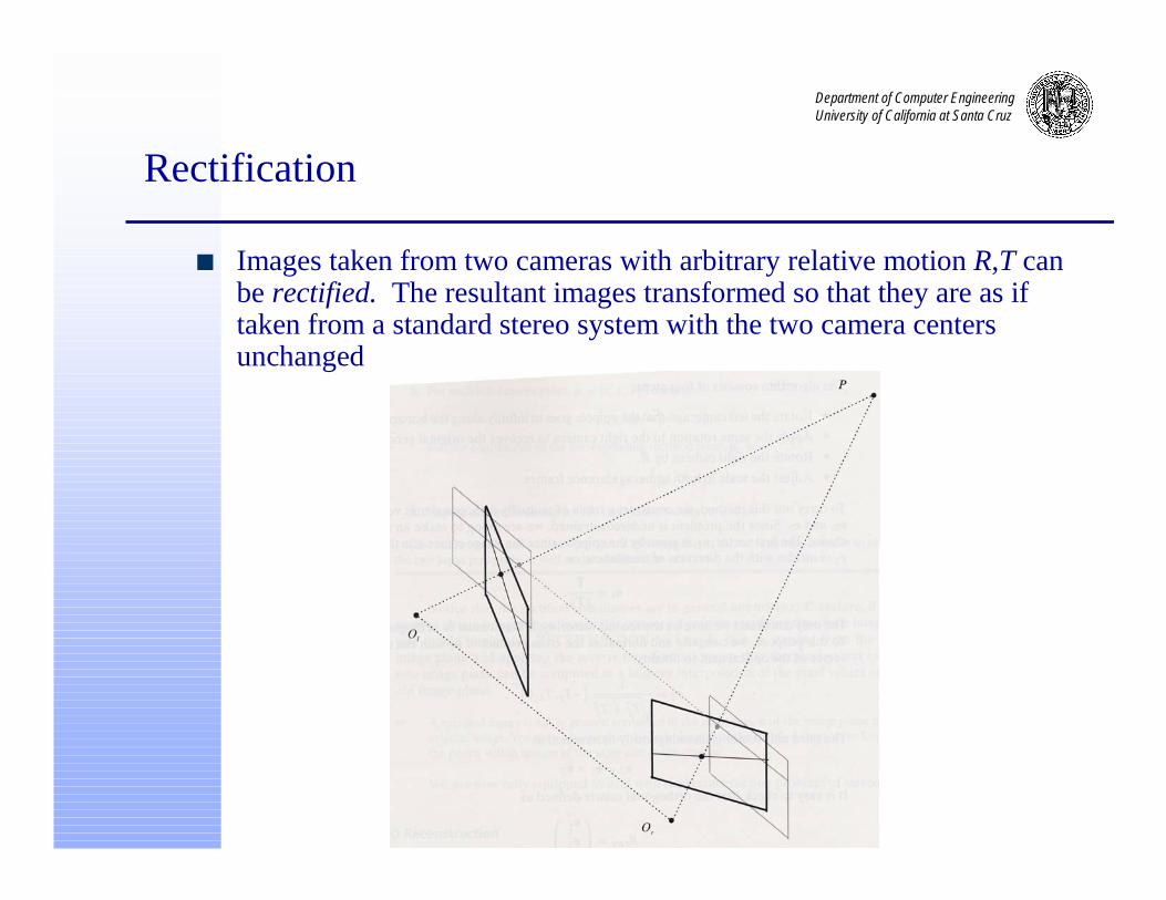
� Images taken from two cameras with arbitrary relative motion R,T can be rectified. The resultant images transformed so that they are as if taken from a standard stereo system with the two camera centers unchanged
Department of Computer EngineeringUniversity of California at Santa Cruz
Image transformation for a rotating camera
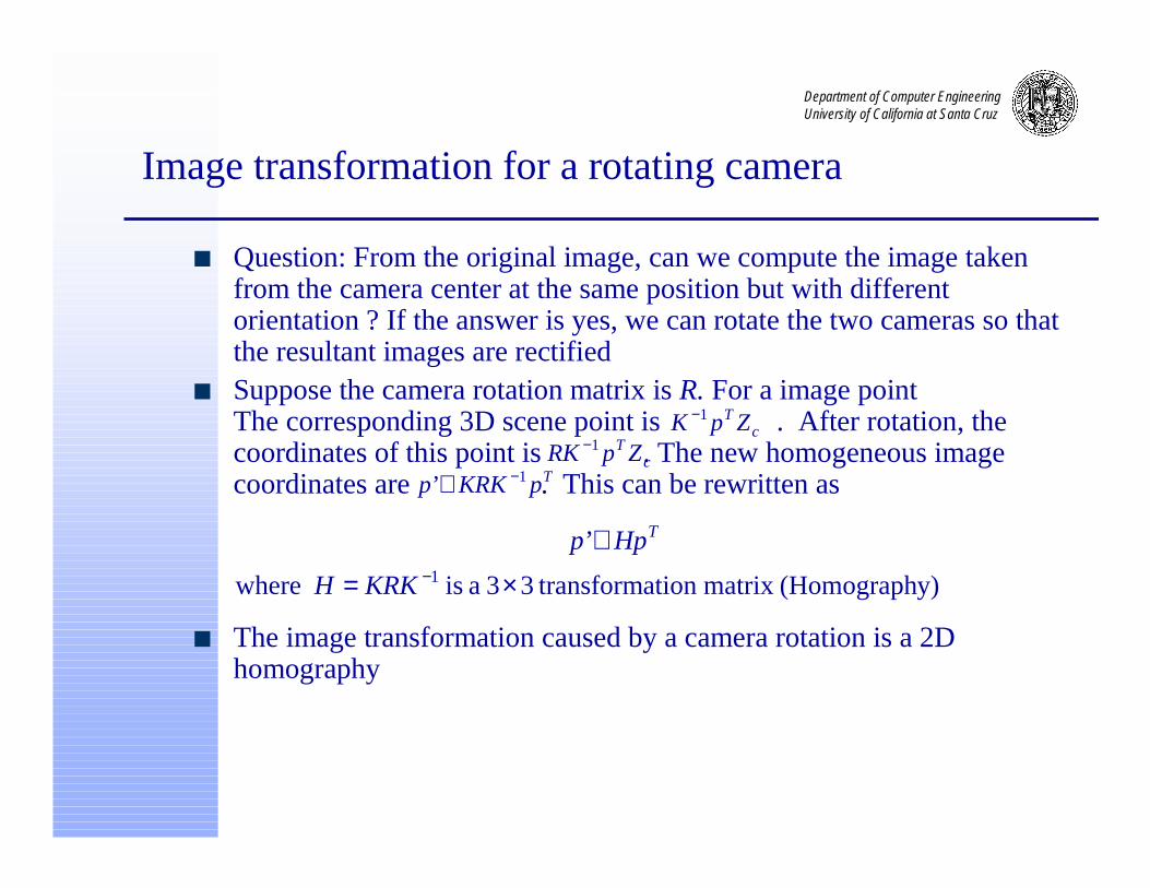
� Question: From the original image, can we compute the image taken from the camera center at the same position but with different orientation ? If the answer is yes, we can rotate the two cameras so that the resultant images are rectified
� Suppose the camera rotation matrix is R. For a image point The corresponding 3D scene point is . After rotation, the coordinates of this point is . The new homogeneous image coordinates are . This can be rewritten as
� The image transformation caused by a camera rotation is a 2D homography
cT ZpK 1−
cT ZpRK 1−
TpKRKp 1’ −≅
y)(Homographmatrix ation transform33 a is where
’ 1 ×=
≅−KRKH
Hpp T
Department of Computer EngineeringUniversity of California at Santa Cruz
Rectification algorithm
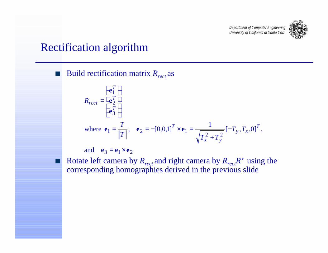
� Build rectification matrix Rrect as
� Rotate left camera by Rrect and right camera by RrectR’ using the corresponding homographies derived in the previous slide
213
22121
3
2
1
and
,]0,,[1
]1,0,0[, where
eee
eee
e
e
e
×=
−+
=×−==
=
Txy
yx
T
T
T
T
rect
TTTTT
T
R

Department of Computer EngineeringUniversity of California at Santa Cruz
Disparity and depth in a simple stereo system
� In a simple/standard binocular stereo system, the correspondences are along the same scan line in the two images. The following figureshows the the relationship between the depth Z and the disparity d=xr-xl
� The following relationship can be easily proved
� The depth is inversely proportionalto the disparity. The closer theobject, the larger the disparity.
� For a scene point at infinity, thedisparity is 0
d
TfZ x=
Department of Computer EngineeringUniversity of California at Santa Cruz
Finding correspondences – correlation-based method
� Assumptions• Most scene points are visible from both viewpoints• Corresponding image regions are similar
� Correlation_matching_algorithmLet pl and pr be pixels in the left and right image, 2W+1 is the width of the correlation window, [-L,L] is the disparity search range in the right image for pl
• For each disparity d in the range of [-L,L] compute the similarity measure c(d)
• Output the disparity with the maximum similarity measure

Department of Computer EngineeringUniversity of California at Santa Cruz
Finding correspondences – correlation-based method

Department of Computer EngineeringUniversity of California at Santa Cruz
Finding correspondences – correlation-based method
� Different similarity measures• Sum of squared differences (SSD)
• Sum of absolution differences (SAD)
• Normalized cross-correlation
2)),(),(()( jyidxIjyixIdc llr
W
Wi
W
Wjlll +++−++−= ∑ ∑
−= −=
|),(),(|)( jyidxIjyixIdc llr
W
Wi
W
Wjlll +++−++−= ∑ ∑
−= −=
∑ ∑
∑ ∑
∑ ∑
−= −=
−= −=
−= −=
+−+++=
−++=
+−+++−++=
=
W
Wi
W
Wjllrllrrr
lll
W
Wi
W
Wjlllll
llrllrlll
W
Wi
W
Wjllllr
rrll
lr
ydxIjyidxIC
yxIjyixIC
ydxIjyidxIyxIjyixIC
CC
Cdc
2
2
)],(),([
)],(),([
)],(),()][,(),([ where
)(

Department of Computer EngineeringUniversity of California at Santa Cruz
Finding correspondences – feature-based method
� Search is restricted to a set of features in two images, such as edges, corners, etc.
� A similarity measure is used for matching features� Constraints such as the uniqueness constraint (each feature can only
have one match) can be used� Algorithm_feature_matching
• Compute the similarity measure between fl and each feature in the right image
• Select the right image feature with the largest similarity measure and ouput the disparity
� Sample similarity measure for line segments
line edge thealongconstrast average the and midpoint,
the n,orientatio the segment, line theoflength theis where
)()()()(
12
32
22
12
0
c
ml
ccwmmwwllwS
rlrlrlrl
θθθ −+−+−+−
=


