Rediscover Predictability: Information from the Relative Prices of Long-term and Short-term Dividends * Ye Li † Chen Wang ‡ November 17, 2017 Abstract The relative prices of dividends at alternative horizons contain critical information on the behavior of aggregate stock market. The ratio between prices of long- and short-term dividends, “price ratio” (pr t ), predicts annual market return with an out- of-sample R 2 of 19%. pr t subsumes the predictive power of traditional price-dividend ratio (pd t ). A modified Gordon (1962) model shows that pr t is more pure a proxy for expected return than pd t , which also contains expected future dividends. Predictability is stronger after market downturns, and holds outside the U.S. As an economic test, shocks to pr t are priced in the cross-section of stocks, consistent with ICAPM. Our measure of expected return declines during monetary expansions, and varies with vari- ables that reflect conditions of macroeconomy, financial intermediaries, and sentiment. * We thank Nick Barberis, Geert Bekaert, Ian Dew-Becker, Jules H. Van Binsbergen, Kent Daniel, Ste- fano Giglio, Will Goetzmann, Ralph S.J. Koijen, Lars A. Lochstoer, Alan Moreira, Tano Santos, Jos´ e A. Scheinkman, and Michael Weber for helpful comments. We are grateful to participants at LBS Transatlantic PhD Conference, and Yale Finance PhD Seminar. All errors are ours. † The Ohio State University. E-mail: [email protected]‡ Yale School of Management. E-mail: [email protected]
Transcript
Rediscover Predictability: Information from the Relative
Prices of Long-term and Short-term Dividends∗
Ye Li† Chen Wang‡
November 17, 2017
Abstract
The relative prices of dividends at alternative horizons contain critical information
on the behavior of aggregate stock market. The ratio between prices of long- and
short-term dividends, “price ratio” (prt), predicts annual market return with an out-
of-sample R2 of 19%. prt subsumes the predictive power of traditional price-dividend
ratio (pdt). A modified Gordon (1962) model shows that prt is more pure a proxy for
expected return than pdt, which also contains expected future dividends. Predictability
is stronger after market downturns, and holds outside the U.S. As an economic test,
shocks to prt are priced in the cross-section of stocks, consistent with ICAPM. Our
measure of expected return declines during monetary expansions, and varies with vari-
ables that reflect conditions of macroeconomy, financial intermediaries, and sentiment.
∗We thank Nick Barberis, Geert Bekaert, Ian Dew-Becker, Jules H. Van Binsbergen, Kent Daniel, Ste-fano Giglio, Will Goetzmann, Ralph S.J. Koijen, Lars A. Lochstoer, Alan Moreira, Tano Santos, Jose A.Scheinkman, and Michael Weber for helpful comments. We are grateful to participants at LBS TransatlanticPhD Conference, and Yale Finance PhD Seminar. All errors are ours.†The Ohio State University. E-mail: [email protected]‡Yale School of Management. E-mail: [email protected]
This paper provides new evidence on stock return predictability. Based on our predictor, the
expected return declines in response to expansionary monetary policy, and varies closely with
variables that reflect the conditions of macroeconomy, financial intermediary, and sentiment.
Moreover, shocks to the expected market return is priced in the cross section of stocks.
Our return predictor is the ratio of long-term dividend price to short-term dividend
price. While great efforts have been made to understand the properties of dividend strips,
especially their average returns (reviewed by Binsbergen and Koijen (2017)), we are the first
to show that the relative dividend prices at alternative horizons contain critical information
on the expected return of aggregate market. We also find stronger return predictability after
the market underperforms the risk-free rate, and our results hold outside the United States.
We start from a simple identity: the total valuation of the market is equal to the sum of
the price of long-term dividends and the price of short-term dividends, so the price-dividend
ratio can be decomposed as follows
PtDt
=Price of Long-term Dividends
Dt
+Price of Short-term Dividends
Dt
.
Using a state-space model, we show that the two components could contain distinct infor-
mation on future returns and dividends. To extract information from the pair that is beyond
the traditional price-dividend ratio (i.e., pdt = ln(PtDt
)), we calculate the ratio of long-term
to short-term dividend prices (“price ratio” or “prt”),
prt = ln
(Price of Long-term Dividends
Price of Short-term Dividends
).
The dividend prices are obtained from derivative markets from January 1988 to June 2017.1
Our price ratio can be interpreted as the slope of term structure of dividend prices,
while the price-dividend ratio (pdt) captures the level. Moreover, prt is a measure of duration.
In our implementation, “short-term” is defined as one year. Using the valuation of dividends
in the coming year as numeraire, prt measures how many years of valuation are there beyond
one year. A high value of prt means that the market has a long duration.
1Binsbergen, Brandt, and Koijen (2012) show that futures or option data can be used to calculate dividendstrip prices. We use futures data, because futures have a longer sample than options. Figure 8 in the appendixshows that prt computed from futures and option data have 88% correlation.
1
We find that prt strongly predicts market return. A decrease of prt by one standard
deviation adds 7.3% to the expected return over the next year. When forecasting annual
returns, prt produces an out-of-sample R2 equal to 19.2%, which is three times the out-of-
sample R2 of pdt in our sample. This degree of variability in return expectations is difficult
to reconcile with state-of-the-art asset pricing models (e.g., Campbell and Cochrane (1999)
and Bansal and Yaron (2004)). The forecasting performance of prt can be directly compared
to that of the many alternative predictors in the literature. Previously studied predictors
typically perform well in-sample but become insignificant out-of-sample, often performing
worse than forecasts based on the historical mean return (Goyal and Welch (2007)).
We establish the robustness of our return prediction results in a number of ways. First,
following Hodrick (1992), we adjust our standard error by taking into account the overlapping
structure of annual returns on the left-hand side of predictive regression. Second, we show
that the autocorrelation of prt is 91.5%, lower than that of pdt (98.7%), and that our estimate
of predictive coefficient is robust to Stambaugh (1999) bias. Ferson, Sarkissian, and Simin
(2003) show a spurious regression bias when both the proposed predictor and the underlying
expected return are persistent. Third, we conduct several out-of-sample tests (e.g., Clark
and McCracken (2001)). Finally, we also show that in terms of in-sample R2, out-of-sample
R2, and Hodrick (1992) t-statistic, prt outperforms all the alternative predictors.
We modify the model of Gordon (1962) to understand the superiority of prt over pdt
as return predictor. The model accommodates news on both expected return and dividend
growth. Specifically, it shows when dividend is not predictable, prt coincides with pdt, and
both predict future returns. The superiority of prt over pdt as a return predictor is due to
the fact that prt isolates the information on the expected return, while the return predictive
power of pdt is compromised by the information it contains on future dividends. Indeed, we
show that after regressing pdt on prt, the residuals strongly forecast dividend growth at one
year horizon with an out-of-sample R2 equal to 30%. In contrast, the dividend predictive
power of prt is very weak. A recent literature proposes variants of growth-adjusted valuation
ratios as return predictor (Campbell and Thompson (2008); Lacerda and Santa-Clara (2010);
Da, Jagannathan, and Shen (2014); Golez (2014)). Our predictor prt does not rely on an
adjustment model. It is obtained directly from market prices of dividend strips.
The price ratio, prt, predicts return outside the United States. We run a panel predic-
tive regression with the future realized return of each country on the left hand side, and prt of
2
each country on the right hand side. The panel predictive coefficient is strongly significant,
and close in magnitude to the coefficient estimated using the U.S. sample. Interestingly, once
time fixed effect is added to absorb the global factor in realized returns, return predictability
disappears, suggesting that the variation of expected stock return across countries tends to
comove, which is in line with Miranda-Agrippino and Rey (2015).
We find that the return predictive power of prt is asymmetric – it is much stronger
following a down market (i.e., negative market excess returns in the past twelve months).2
Such asymmetry holds outside the United States. We evaluate two asset pricing models
(Barberis, Huang, and Santos (2001) and He and Krishnamurthy (2013)) that produce strong
asymmetry in return predictability. While the return predictive power of prt depends on the
state variables proposed by both models, these state variables alone do not predict future
returns as implied by the theories.
The results of conditional return prediction suggest that the expected return is a func-
tion of both prt and past returns. Thus, our findings are related to the long-standing liter-
ature on return autocorrelation (Fama and French (1988); Poterba and Summers (1988)).
When prt is at its mean, return does not show autocorrelation. However, when prt is one
standard deviation (or more) above the mean, return exhibits momentum at one year horizon,
and when prt is one standard deviation (or more) below the mean, return shows reversal.
The impact of monetary policy on asset prices continues attracting enormous attention
(Lucca and Moench (2015); Campbell, Pflueger, and Viceira (2015)). Using prt as a proxy for
the expected return, we show that the expected return declines in response to expansionary
monetary policy. Specifically, we regress prt on the unanticipated changes in Federal Funds
rate that are calculated following Cochrane and Piazzesi (2002), and find a negative shock to
the policy rate (monetary easing) is associated with an increase in prt, and thus, a decrease
in the expected stock return. In contrast, the level of price-dividend ratio, a typical proxy
for expected return (e.g., Muir (2017)), does not respond to monetary policy shocks. We
also find that monetary easing tends to be associated with higher contemporaneous return,
in line with Thorbecke (1997) and Bernanke and Kuttner (2005). Thus, stock price rises
in response to expansionary monetary policy, but since the expected return declines, such
increase tends to revert over the next year. We proxy the expected dividend growth by the
2Rapach, Strauss, and Zhou (2010), Henkel, Martin, and Nardari (2011), Dangl and Halling (2012), andCujean and Hasler (2017) find that return predictors, such as the price-dividend ratio, have better predictivepower in economic downturns.
3
regression residual of pdt with respect to prt, and find it does not respond to monetary policy
shocks.
Next, we show that the expected stock return, calculated from unconditional and con-
ditional predictive regressions, varies with business conditions, broker-dealer balance sheets,
uncertainty, and sentiment. The expected return is positively correlated with unemployment
and term spread, and negatively correlated with consumption growth, fixed investment, and
inflation. The expected return shows a very strong negative correlation with broker-dealer
leverage (Adrian and Shin (2010)) and a positive correlation with broker-dealer CDS spreads,
a proxy for under-capitalization. Interestingly, the expected return declines when VIX rises,
which has important implications on the dynamics of risk-return trade-off (Lettau and Lud-
vigson (2010)).3 The expected return tends to be low when the sentiment (Baker and Wurgler
(2006)) is high, even after the sentiment index is orthogonalized to macro variables.
Last but not least, we estimate the price of risk for shocks to prt. If prt is a valid
return predictor, shocks to it are shocks to the expected market return. By the logic of
ICAPM, shocks to investment opportunity set are priced. Therefore, estimating the price of
prt risk is an economic test of prt as a return predictor. Using characteristic-sorted portfolios
as the asset universe, we find a negative and statistically significant price of prt risk. Two
assets with one standard deviation difference in their prt beta have 2.1% difference in average
annual returns. In contrast, few existing studies on return predictors conduct this economic
test, and most studies solely rely statistical tests to establish return predictive power.
The reminder of the paper is organized as follows. Section 2 shows variable construction
and documents the evidence of return predictability (in and outside the United States) when
prt is used as predictor. This section also shows that the residual of pdt after regressing on
prt strongly predicts dividend growth. We provide a simple model in Section 2.4 to reconcile
the evidence. Section 3 provides the evidence on the asymmetry of return predictability (in
and outside the United States), and an evaluation of related theories. Section 4 provides
evidence on how monetary policy affects the expected return, and how the expected return
varies with macro and financial variables. It closes with the estimation of price of prt risk.
Section 4 concludes. Derivation and additional results are provided in the appendices.
3VIX may not reflect the risk from variation in the investment opportunity set, which can be a importantcomponent of risk (Guo and Whitelaw (2006)).
4
2 Return Prediction
This section starts with a state space model of return and cash flow that shows the price-
dividend ratio (“pdt”) as a compression of information on future return and dividends. To
release the information trapped in pdt, we decompose market price into the prices of long- and
short-term dividends, and calculate the ratio of the former to the latter, i.e., the “price ratio”
(prt). Table 1 compares summary statistics of pdt and prt, and in particular, shows that pr
is much less persistent. Table 2 shows the return predictive power of prt, which is much
stronger that pdt’s. The improvement is likely from prt’s high-frequency variation (Figure
1), and the fact that pdt mixes the information on expected return and dividend growth.
Table 3 shows that the regression residuals of pdt with respect to prt strongly predicts future
dividends. We show that prt forecasts returns outside of the United States (Table 4), and it
outperforms other predictors in out-of-sample R2 and Hodrick (1992) t-statistics (Figure 3).
2.1 Decomposing the price-dividend ratio
State space model. We consider a state space model of return and cash flow growth (e.g.,
Cochrane (2008)). Let µt denote the expected return from time t to t+1, and gt the expected
dividend growth. We assume that the information set at time t is summarized by factors Ft,
and the expected return and dividend growth are given by the following linear system4
µt = γ0 + γ ′Ft,
gt = δ0 + δ′Ft.(1)
Following Binsbergen and Koijen (2010) and Kelly and Pruitt (2013), we impose a VAR(1)
structure on the factors
Ft+1 = ΛFt + ξt+1, (2)
where Λ is a constant matrix with conformable dimensions. Let pdt denote the log price-
dividend ratio of the market at time t, ∆dt+j the one-period dividend growth from t+ j − 1
to t + j, and rt+j the market return from t + j − 1 to t + j. We can use the present value
4A non-linear model is more general, but this model is only used for the purpose of motivation, notestimation.
5
identity of Campbell and Shiller (1988), i.e.,
pdt =κ
1− ρ +∞∑j=1
ρj−1Et [∆dt+j − rt+j] , (3)
to solve the price-dividend ratio as a function of Ft:
pdt = φ0 + φ′Ft, (4)
where φ0 is equal to κ+δ0−γ01−ρ , and φ′ is equal to ιψ′ (1− ρΛ)−1 with ι being a row vector
(1,−1) and ψ equal to (δ′,γ ′). Derivation details are in Appendix I.
By linking the price-dividend ratio to future returns and dividend growth, the present
value identity serves as a motivation to use pdt as a predictor. Yet, the factor structure
reveals that any predictive power of pdt comes from a particular linear combination of Ft,
i.e., a compression of information. Therefore, we should be able to release the trapped
information by decomposing the price-dividend ratio into different components with distinct
information content from Ft. Next, we consider a decomposition along cash-flow horizon.
The Price Ratio. Let St denote ex-dividend market value, Dt, the dividend at t, and rt,
the short rate. Under the no-arbitrage condition, there exists a risk-neutral measure, Q, such
that the stock price is a sum of the expected future dividends discounted by the cumulative
short rates:
St =∞∑τ=1
EQt[e−
∫ t+τt rsdsDt+τ
]=
T∑τ=1
EQt[e−
∫ t+τt rsdsDt+τ
]︸ ︷︷ ︸
PT−t
+∞∑
τ=T+1
EQt[e−
∫ t+τt rsdsDt+τ
]︸ ︷︷ ︸
PT+t
,
where P T−t is the price of dividends paid from t + 1 to t + T , i.e., the price of short-term
dividends, and P T+t is the price of long-term dividends. Dividing both sides by Dt, we obtain
a decomposition of price-dividend ratio into two valuation ratios, i.e., the ratio of short-term
dividend price to Dt, and the ratio of long-term dividend price to Dt:
StDt
=P T−
Dt
+P T+
Dt
. (5)
While the price-dividend ratio is the sum of these two valuation ratios, we construct
6
our predictor by taking the (log) difference so that it may reflect different information from
the pair(PT−
Dt, P
T+
Dt
):
prt = ln
(P T+
Dt
)− ln
(P T−
Dt
)= ln
(P T+
P T−
)(6)
Our predictor “prt” is a price ratio, the log ratio of long-term dividend price to short-term
dividend price. We use the log difference instead of level difference to get rid of Dt, so that
prt has market prices in both its numerator and denominator, and thereby, captures the
variation of expected return at relatively higher frequencies than pdt. In the literature, and
as in this paper, the current dividend Dt is measured by the sum of dividends paid in the
previous year to remove seasonality (Fama and French (1988)), so through Dt, pdt tends to
be more sluggish than prt, and thus, less responsive to the current conditions of financial
markets and the real economy.
Together, pdt and prt should reflect the information content of(PT+
Dt, P
T−
Dt
). Our em-
pirical results will show that our price ratio prt is a better way to extract information about
future returns than the traditional price-dividend ratio. Intuitively, the valuation of long-
term dividends is more sensitive to discount rate movements than the valuation of short-term
dividends. The ratio of the former to the latter tends to increase when the discount rate
declines, and decrease when the discount rate rises.
To construct prt, we need the short-term dividend price and the long-term dividend
price, which are calculated using data of S&P 500 futures and zero-coupon bonds (ZCBs) as
follows.5 Consider any T > 0. To calculate P T+t from futures price and ZCB price, we make
the assumption that∫ t+Tt
rsds and St+T are not correlated under Q measure, so we have
P T+t =
∞∑τ=T+1
EQt[e−
∫ t+Tt rsdse−
∫ t+τt+T rsdsDt+τ
]= EQt
[e−
∫ t+Tt rsdsEQt+T
[∞∑
τ=T+1
e−∫ t+τt+T rsdsDt+τ
]︸ ︷︷ ︸
St+T
]
=EQt[e−
∫ t+Tt rsdsSt+T
]= EQt
[e−
∫ t+Tt rsds
]︸ ︷︷ ︸
ZCBTt
EQt [St+T ] . (7)
Therefore, we can calculate P Tt directly from the price of ZCB that matures in T periods,
5Figure 8 shows that prt from futures has 88% correlation with prt from options in Binsbergen, Brandt,and Koijen (2012).
7
Table 1: Summary Statistics
This table reports the number of observations, mean, standard deviation, mininum, maximum, quartiles,and first-order (one-month) autocorrelation (ρ) of our predictor, prt (the ratio of long-term dividend priceto short-term dividend price) and pdt (the price-dividend ratio). The correlation matrix is shown at the endof the table. Using Equation (7), we construct long-term dividend price from data of S&P 500 futures priceand zero-coupon bond price (source: Bloomberg), and short-term dividend price is the difference betweenS&P 500 index value and long-term dividend price. pdt is the month-end price-to-dividend ratio of S&P 500index (source: Bloomberg).
ZCBTt , and futures price that is the Q-expectation of future stock price (Duffie (2001)).
2.2 Predicting return
Data and summary statistics. To construct prt, we use monthly data of S&P 500
futures (source: Bloomberg) and zero-coupon bond prices (source: Fama-Bliss database)
from January 1988 to June 2017.6 pdt is the month-end price-dividend ratio of S&P 500
index (source: Bloomberg). We set T equal to one year, so prt is the log ratio of price of
dividends paid beyond the coming year to price of dividends paid within the the coming
year. Accordingly, we focus on forecasting the return of S&P 500 index at one-year horizon,
but also report the forecasting results at one-month horizon in the appendix. The sample
starts in 1988 because the stock market crash in October 1987 reveals anomalous trading
behavior in the futures market that was largely driven by portfolio insurance (Brady Report
(1988)). After the crash, regulators overhauled several trade-clearing protocols.7
Table 1 reports the summary statistics of prt, and log price-dividend ratio pdt for com-
parison. We can interpret prt as a measure of duration. Its median value, 3.992, translates
into 54.2 after taking exponential, meaning that the valuation of dividends in all the years
after the coming year is 54.2 times the valuation of dividends in the coming year. In other
words, the market has a valuation duration of a total 55.2 years. prt has a wide range of
6Available maturities vary over time, so to obtain futures at constant maturities, such as one year, weneed to interpolate data. We use shape-preserving piecewise cubic interpolation to preserve the shape of thefutures curve.
7According to the New York Stock Exchanges current website: “In response to the market breaks inOctober 1987 and October 1989, the New York Stock Exchange instituted circuit breakers to reduce volatilityand promote investor confidence. By implementing a pause in trading, investors are given time to assimilateincoming information and the ability to make informed choices during periods of high market volatility.”
8
variation, with a minimum of 2.677 (i.e., 15.5 years) right before the 1990-1991 recession
(Jun. 1990) and a maximum of 6.631 (i.e., 759.2 years) near the end of dot-com boom (Nov.
2000).
prt has a lower one-month autocorrelation (“ρ”) than pdt. The persistence of predictors
is a major concern in the literature on return forecasting, especially due to the associated
small-sample bias (Nelson and Kim (1993); Stambaugh (1999)) and spurious regression when
the underlying expected return is persistent (Ferson, Sarkissian, and Simin (2003)).
The correlation between prt and pdt is 0.87. As will be shown later by the cross-
spectrum in Figure 1, the high correlation is mainly from low frequency movements. When
forecasting the market return, we will consider pdt and prt separately as univariate predictors,
and also examine the predictive power of the residual of prt after regressing on pdt and that
of the residual of pdt after regressing on prt.
Inference and forecasting evaluation. We run the following regression to predict one-
year return:
rt,t+12 = α + βxt + εt,t+12, (8)
where xt is a predictor. Twelve-month forecasts use overlapping monthly data, so we ad-
just our standard errors to reflect the dependence that overlap introduces into error terms.
Following Cochrane and Piazzesi (2002), we report Newey and West (1987) standard errors
with 18 lags to account for the moving-average structure induced by overlap. Besides, we
also calculate Hodrick (1992) standard errors. Hodrick (1992) shows that GMM-based auto-
covariances correction (e.g., Newey and West (1987)) can have poor small-sample properties,
Related to the serial correlation in errors, another concern is the persistence of predictor that
induces bias in β estimate. We report the estimate adjusted for Stambaugh (1999) bias.
The adjusted R2 measures in-sample fitness. Several studies have raised concerns over
out-of-sample performances of return predictors (Bossaerts and Hillion (1999); Goyal and
Welch (2007)). To address these issues, we report the out-of-sample R2 and two formal tests
of out-of-sample performances. We calculate out-of-sample forecasts from the perspective
of a real-time investor, using data up to time t in the predictive regression to obtain the
coefficient β, which is then multiplied by the time-t value of the predictor to form the
forecast. Out-of-sample forecasting start from December 1997, when we have at least ten
9
years of data. Out-of-sample R2 is defined by
R2OOS = 1−
∑t (rt,t+12 − rt,t+12)
2∑t (rt,t+12 − rt)2
,
where rt,t+12 is the forecast value and r is the average of twelve-month returns (the first
return is January-December 1998). The out-of-sample R2 lies in the range (−∞, 1], where a
negative number means that a predictor provides a less accurate forecast than the return’s
historical mean.
We report the p-value of two tests of out-of-sample performance, “ENC” and “CW”.
ENC is the encompassing forecast test derived by Clark and McCracken (2001), which
is widely used in the forecasting literature. We test whether the predictor has the same
out-of-sample forecasting performance as the historical mean, and compare the value of the
statistic with critical values calculated by Clark and McCracken (2001) to obtain a range of
p-value. Besides, Clark and West (2007) adjust the standard MSE t-test statistic to produce
a modified statistic (CW ) that has an asymptotic distribution well approximated by the
standard normal distribution, so for CW , we report the precise p-value.
One-year return prediction. Table 2 presents the results of annual return forecasting.
Column (1) shows that our price ratio, prt, demonstrates a striking degree of predictabil-
ity for one-year returns. The in-sample implementation generates a predictive R2 reaching
23.8%.8 Out-of-sample forecasts are similarly powerful, delivering an R2 of 19.2%, signifi-
cantly outperforming the historic mean as shown by the p-values of ENC and CW .
Campbell and Thompson (2008) calculate a long-term estimate of the market Sharpe
ratio (“s0”) equal to 0.374. In the Appendix (see also Kelly and Pruitt (2013)), we show
that the Sharpe ratio of a mean-variance investor’s market-timing strategy (“s1”) is related
to s0 through s1 =
√s20 +R2
1−R2, where R2 is the out-of-sample R2 when prt is used as annual
return predictor. Therefore, an out-of-sample R2 of 19.2% (Table 2) implies a Sharpe ratio of
0.84, suggesting that the stochastic discount factor is more volatile than what is implied by
state-of-art structural asset pricing models (e.g., Campbell and Cochrane (1999) and Bansal
8Foster, Smith, and Whaley (1997) discuss the potential data mining issues that arises from researcherssearching among potential regressors. They derive a distribution of the maximal R2 when k out of mpotential regressors are used as predictors, and they calculate the critical value for R2, below which theprediction is not statistically significant. For instance, when m = 50, k = 5, and the number of observationsis 250, the 95% critical value for R2 is 0.164.
10
Table 2: One-year Return Prediction
This table reports the results of predictive regression (Equation (8)). The left-hand side variable is the returnof S&P 500 index in the next twelve months. We consider four the right-hand side variables (i.e., predictors),
prt, pdt, the residuals of prt after regressing on pdt (εprt ), and the residuals of pdt after regressing on prt (εpdt ),and the results are reported in Column (1) to (4) respectively. The β estimate is shown followed by Neweyand West (1987) t-statistic (with 18 lags), Hodrick (1992) t-statistic, the coefficient adjusted for Stambaugh(1999) bias, and the in-sample adjusted R2. We run the regression monthly. Starting from December 1997,we form out-of-sample forecasts of return in the next twelve months by estimating the regression with data upto the current month, and use the forecasts to calculate out-of-sample R2, ENC test (Clark and McCracken(2001)), and the p-value of CW test (Clark and West (2007)).
The predictive coefficient is also large in magnitude, indicating a high volatility of
expected return. An decrease of prt by one standard deviation adds 7.3% to the expected
return. Both Newey-West and Hodrick t-statistics are significant at least at the 1% level.
Column (2) reports the results for pdt. The return predictive power of pdt is weaker
than prt in all aspects. Its in-sample and out-of-sample R2 is almost half of those of prt.
Its coefficient is smaller and less significant. In the appendix (Figure 9), we show that the
predictive coefficient of pdt is also less stable than prt. Moreover, an decrease in pdt by one
standard deviation leads to an increase of expected return by 5.8%, implying a less volatile
expected return than the one from prt.
Since prt and pdt are highly correlated, we regress prt on pdt to obtain residuals, εprt ,
that are orthogonal to pdt in sample, and use the residual as a predictor to evaluate the return
predictive power of prt beyond pdt. The results are reported in Column (3). prt residual still
delivers in-sample and out-of-sample R2 of 9%, showing a very strong incremental predictive
power of prt. Note that to obtain out-of-sample forecasts, at time t we obtain the residuals
11
1m 1w 1d2d3d5dfrequency
101
102
103
104
105
pow
ersp
ectr
ald
ensi
ty
Dailly sampling power spectral density
prtpdt
εprt
1m 1w 1d2d3d5dfrequency
101
102
103
104
105
cros
ssp
ectr
ald
ensi
ty
Dailly sampling cross spectral density
cross spectral density (prt, pdt)
10y 1y 1m0.5y 3mfrequency
102
103
104
105
106
107
108
pow
ersp
ectr
ald
ensi
tyMonthly sampling power spectral density
prtpdt
εprt
10y 1y 1m0.5y 3mfrequency
102
103
104
105
106
107
108
cros
ssp
ectr
ald
ensi
ty
Monthly sampling cross spectral density
cross spectral density (prt, pdt)
Figure 1: Spectrum and Cross-spectrum of Price Ratio and Price-Dividend Ratio. The leftpanel shows the estimated spectral densities of prt, pdt, and the residuals of prt after regressing on pdt(εprt). The integral of spectral density is equal to the variance. The horizontal line starts from zero andends at π, but labeled with the corresponding length of a cycle. The right panel shows the cross-spectraldensity between prt and pdt. The integral of cross-spectral density is equal to the covariance.
εprt only using data up to t from the regression of prt on pdt, and then use these residuals
to estimate the predictive regression. In Column (4), we report the prediction results of εpdt ,
the residuals from regressing pdt on prt. pdt residuals do not exhibit return predictive power,
which again confirms prt as a superior predictor.
Variation in frequency domain. To better understand the incremental predictive power
of prt beyond pdt, Panel A of Figure 1 shows the spectrum of prt, pdt, and εprt , the residuals
from regressing prt on pdt. The area under spectrum, i.e., the integral, is the variance,
so the spectrum graph provides a variance decomposition in the frequency domain. On the
horizontal axis, instead of showing the frequencies from zero to π, we mark the corresponding
length of cycle for easier interpretation. Consistent with the fact that prt is less persistent
than pdt, its variation is also much more concentrated in higher frequencies than the variation
of pdt, and once orthogonalized with respect to pdt, prt’s residual varies mainly at frequencies
higher than one year. Panel B plots the cross-spectrum of prt and pdt. The integral of cross-
spectrum density is the covariance between prt and pdt. The high correlation between prt
and pdt is mainly from low frequencies. This again indicates that it is the high-frequency
variation in prt that has strong return predictive power beyond pdt.
Expected return dynamics. Figure 2 plots the realized market return, the in-sample
12
1989 1994 1999 2004 2009 2014Date
−0.4
−0.2
0.0
0.2
0.4
pr
Real value
IS fit, R2=0.24
OOS fit, R2=0.19
1989 1994 1999 2004 2009 2014Date
−0.4
−0.2
0.0
0.2
0.4
pd
Real value
IS fit, R2=0.16
OOS fit, R2=0.07
Figure 2: Expected Return Dynamics. The graph reports the in-sample fitted value, the out-of-sampleforecast, and the realized twelve-month return of S&P 500 index. The date on horizontal axis is the beginningdate of the twelve-month period. Starting from December 1997, we form out-of-sample forecasts of returnin the next twelve months by estimating the predictive regression with data up to the current month.
fitted value, and the out-of-sample forecast. The horizontal axis shows the beginning date of
each twelve-month return, i.e. the time when the expectation is formed. As before, out-of-
sample forecasts at time t only uses data up to time t to estimate the predictive coefficient.
The out-of-sample forecasting starts from December 1997 when we have at least ten years
of data. We plot separately the expected return from prt and that from pdt. For both
predictors, in-sample versus out-of-sample expected return estimates are fairly consistent
with each other.
The first conclusion we draw from this graph is that in contrast to pdt, which produces
a very smooth expected return over time, prt reveal variations of expected return at higher
frequencies. This observation is consistent with the Figure 1, and the fact that pdt is more
persistent than prt. prt is more responsive to news, as it contains only the market prices
of short-term and long-term dividends. In contrast, pdt has a denominator that is a rolling
accumulation of past dividends. As shown in Table 2, the high-frequency variation (captured
13
by εprt ) is the main reason that prt outperforms pd in return forecasting.
Our sample has three recession periods (shaded). Near the end of recessions, the
expected return tends to increase, which is in line with studies that document countercyclical
equity premium (e.g., Fama and French (1989); Ferson and Harvey (1991)). Related to the
high-frequency variation revealed by prt, such increase is sharper for the expected return
from prt than that from prt. Another interesting fact is that in the year leading up to dot-
com burst and the global financial crisis, the expected return from prt exhibits slump, while
the expected return from pdt barely moves. While the expected return from prt starts to
recover near the end of these recessions, while the expected return from pdt only shows a
smooth upward trend throughout the recession. These new patterns from prt as a proxy for
expected return are very informative for constructing macro-finance models that speaks to
both asset pricing and business-cycle fluctuations.
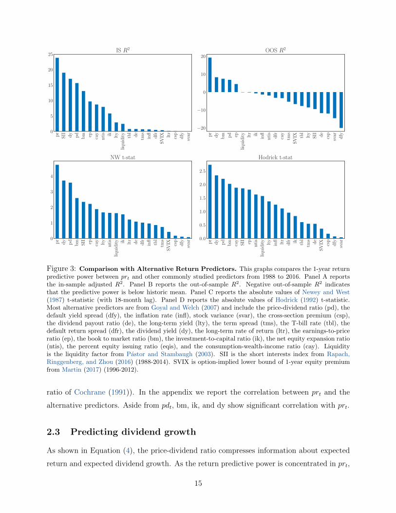
Other predictors. How do our market return forecasts compare with predictors proposed
in earlier literature? Figure 3 compares the predictive accuracy of our approach with an
extensive collection of alternative predictors considered in the literature. In the caption,
we document the sources of these predictors. In particular, we explore forecasts from 18
alternative predictors including the price-dividend ratio (pd), the default yield spread (dfy),
the inflation rate (infl), stock variance (svar), the cross-section premium (csp), the dividend
payout ratio (de), the long-term yield (lty), the term spread (tms), the T-bill rate (tbl), the
default return spread (dfr), the dividend yield (dy), the long-term rate of return (ltr), the
earnings-to-price ratio (ep), the book to market ratio (bm), the investment-to-capital ratio
(ik), the net equity expansion ratio (ntis), the percent equity issuing ratio (eqis), and the
consumption-wealth-income ratio (cay), liquidity factor (liquidity), the short interests index
(SII), the option-implied lower bound of 1-year equity premium (SVIX). Most predictors
are studied in a return predictability survey by Goyal and Welch (2007), and others are
proposed more recently, such as short interest index (“SII” in Rapach, Ringgenberg, and
Zhou (2016)) and SVIX (Martin (2017)). We report in-sample (“IS”) R2, out-of-sample
(“OOS”) R2, the absolute values of Newey-West and Hodrick t-statistics. In our sample,
prt outperforms other predictors in all aspects. Among the alternatives, the price-dividend
ratio and the book-to-market ratio (“bm”) deliver the most successful univariate forecasts,
while others either fail in the out-of-sample R2 (e.g., cay, the consumption-wealth ratio of
Lettau and Ludvigson (2001)) or in statistical significance (e.g., ik, the investment-capital
14
pr
SII dy
pd
bm ep cay
nti
s ik lty
liqu
idit
y
tbl
de
tms
infl
dfr
SV
IX ltr
csp
dfy
svar
0
5
10
15
20
25IS R2
pr
dy
bm pd ep
liqu
idit
y
ltr ik
infl
nti
s
dfr
cay
tms
SV
IX tbl
lty
SII de
csp
svar dfy
−20
−10
0
10
20OOS R2
pr
dy
pd
bm SII ep cay
lty
nti
s
liqu
idit
y ik ltr
de
dfr
infl
tbl
tms
SV
IX csp
dfy
svar
0
1
2
3
4
NW t-stat
pr
dy
pd
bm
cay
SII ep
nti
s
liqu
idit
y
lty
infl ltr
dfr ik tbl
tms
de
SV
IX csp
dfy
svar
0.0
0.5
1.0
1.5
2.0
2.5
Hodrick t-stat
Figure 3: Comparison with Alternative Return Predictors. This graphs compares the 1-year returnpredictive power between prt and other commonly studied predictors from 1988 to 2016. Panel A reportsthe in-sample adjusted R2. Panel B reports the out-of-sample R2. Negative out-of-sample R2 indicatesthat the predictive power is below historic mean. Panel C reports the absolute values of Newey and West(1987) t-statistic (with 18-month lag). Panel D reports the absolute values of Hodrick (1992) t-statistic.Most alternative predictors are from Goyal and Welch (2007) and include the price-dividend ratio (pd), thedefault yield spread (dfy), the inflation rate (infl), stock variance (svar), the cross-section premium (csp),the dividend payout ratio (de), the long-term yield (lty), the term spread (tms), the T-bill rate (tbl), thedefault return spread (dfr), the dividend yield (dy), the long-term rate of return (ltr), the earnings-to-priceratio (ep), the book to market ratio (bm), the investment-to-capital ratio (ik), the net equity expansion ratio(ntis), the percent equity issuing ratio (eqis), and the consumption-wealth-income ratio (cay). Liquidityis the liquidity factor from Pastor and Stambaugh (2003). SII is the short interests index from Rapach,Ringgenberg, and Zhou (2016) (1988-2014). SVIX is option-implied lower bound of 1-year equity premiumfrom Martin (2017) (1996-2012).
ratio of Cochrane (1991)). In the appendix we report the correlation between prt and the
alternative predictors. Aside from pdt, bm, ik, and dy show significant correlation with prt.
2.3 Predicting dividend growth
As shown in Equation (4), the price-dividend ratio compresses information about expected
return and expected dividend growth. As the return predictive power is concentrated in prt,
15
Table 3: Dividend Growth Prediction
This table reports the results of dividend growth forecasting regression. The left-hand side variable is theone-year, non-overlapping dividend growth rate of S&P 500 index defined in Equation (10). We consider
four the right-hand side variables (i.e., predictors), the residuals of pdt after regressing on prt (εpdt ), pdt, prt,
the equity yield (ln(
Dt
PT−t
)), and the results are reported in Column (1) to (4) respectively. The estimated
predictive coefficient (β) is shown followed by Newey and West (1987) t-statistic (with 18 lags), Hodrick(1992) t-statistic, the coefficient adjusted for Stambaugh (1999) bias, and the in-sample R2. We run theregression monthly. Starting from December 1997, we form out-of-sample forecasts of return in the nexttwelve months by estimating the regression with data up to the current month, and use the forecasts tocalculate out-of-sample R2, ENC test (Clark and McCracken (2001)), and the p-value of CW test (Clarkand West (2007)).
εpdt pdt prt ln(
DtPT−t
)β 0.307 0.014 -0.035 -0.127
Newey-West t (3.204) (0.247) (-2.005) (-3.395)Hodrick t [5.153] [0.642] [-3.990] [-6.767]Stambaugh bias adjusted β 0.316 0.025 -0.024 -0.118
the component of pdt that is orthogonal to prt (i.e., εpdt ) should forecast dividend growth. We
measure dividend growth by the ratio of adjacent, non-overlapping cumulative dividends,
∆Dt,t+12 =
∑12i=1Dt+i∑12
i=1Dt−12+i.9 (9)
In the predictive regression, we use the logarithm of ∆Dt,t+12 as the forecasting target.
Table 3 reports the results of dividend growth prediction.10 Column (1) shows that
εpdt , the residual of pdt after regressing on prt, exhibits very strong predictive power with
in-sample and out-of-sample R2 of 34.9% and 30.4% respectively. The coefficient has a
large magnitude and is statistically significant. One standard-deviation increase of εpdt is
associated with 4.55% increase of dividend growth (i.e., 3.7 standard deviations). Column
(2) shows that pdt itself does not strongly predict dividend growth. Together, Table 2 and 3
9Dividends are calculated from the difference between cum- and ex-dividend S&P index levels.10Forecasting dividend growth has been at the center of asset pricing literature (see Ball and Watts (1972),
Campbell and Shiller (1988), Cochrane (1992), Fama and French (2000), Lettau and Ludvigson (2005), Koijenand van Nieuwerburgh (2011), Lacerda and Santa-Clara (2010) and Golez (2014)).
16
show that the information about future return and dividend is mingled together in pdt. Such
information is disentangled, once pdt is decomposed by cash-flow horizon, and the price ratio
prt is constructed to capture the information about expected return. Column (3) shows that
in comparison with εpdt , the dividend predictive power of prt is weaker, with an out-of-sample
R2s only 15% of the out-of-sample R2 of εpdt . Thus, the decomposition of pdt into prt and
εpdt adequately separates the information on expected return and dividend growth.
Our analysis of return and dividend predictability echoes the observation of Cochrane
(2007) that price-dividend ratio must either predict return or dividend growth. Our results
show an even richer story: the predictive information on return and dividend cancels out
each other within pdt. Once we distill the information on future return, the rest of pdt
has a much stronger dividend forecasting power than pdt itself. The intuition behind this
result is related to the countercyclicality of expected return. When the economy is booming
and dividend grows fast, expected return tends to be low, and when dividend grow slowly,
expected return tends to be high. Through the lens of our state space model, the factors
that drive expected return and dividend growth have strong correlation with each other, so
when combined together in pdt, they cancel each other out.
εpdt is closely related to the “equity yield” in Binsbergen, Hueskes, Koijen, and Vrugt
(2013), especially its dividend predictive power. Following that paper, we define equity yield
as ln(
DtPT−t
), i.e., the log ratio of past dividend to short-term dividend price. The following
equation directly decomposes pdt into prt and the equity yield:
pdt = ln (1 + eprt)− ln
(Dt
P T−t
)≈ κ0 + κ1prt − κ2 ln
(Dt
P T−t
), (10)
where the linearizion coefficients are κ1 = exp(pr)
1+exp(pr), κ2 = 1, and κ0 = ln
(1 + exp (pr)
)−κ2pr.
The upper bar represents long-run means, around which we log-linearize the equation. The
correlation between prt and the equity yield is 0.86 in our sample, so Equation (10) is only an
imperfect decomposition. As shown in Column (4) of Table 3, the equity yield also predicts
dividend growth, albeit with a forecasting power less than εpdt .11
11Our sample length differs from Binsbergen, Hueskes, Koijen, and Vrugt (2013) (October 2002 and April2011), who use dividend derivatives to derive short-term dividend prices, so the estimates of predictivecoefficient are different.
17
2.4 A simple model
The intuition behind our results on return and dividend growth predictability can be under-
stood through a very simple model. Following Gordon (1962) and Campbell and Thompson
(2008), we consider a stationary economy. Each period is index by t, and t = 0, 1, 2, ... Let
D0 denote the dividend paid in period 0. At the beginning of period 1, news about future
discount rate and dividend are revealed so that from now on, the economy jumps at a new
steady state with a constant discount rate r and a constant dividend D1. Therefore, the
stock price is
P =+∞∑t=1
D1
(1 + r)t=D1
r,
and the prices of short-term dividends (paid within period 1) and long-term dividends (paid
after period 1) are respectively
P− =D1
1 + r,
and
P+ =+∞∑t=2
D1
(1 + r)t=
D1
r (1 + r).
Our price ratio, pr, is precisely the negative logarithm of the expected return r,
pr = ln
(P+
P−
)= ln
(D1
r(1+r)
D1
1+r
)= − ln (r) , (11)
so naturally, pr predicts the future stock market return as documented in Table 2.
We can also calculate the price-dividend ratio
pd = ln
(D1/r
D0
)= − ln (r) + ln
(D1
D0
)= pr + g,
where g is the log dividend growth rate. Therefore, pd is an imperfect proxy for the expected
return, as it also contains information about dividend growth. Moreover, the residual of pd
with respect to pr reflects the information on dividend growth as documented in Table 3. pd
and pr are identical only if D1 = D0 (or dividend growth g = 0). This observation is in line
with the state space model that motivates our decomposition of pd on the cash-flow horizon.
It has been shown that information regarding future dividends compromises the return
predictive power of price-dividend ratio (e.g., Menzly, Santos, and Veronesi (2004); Lettau
18
and Ludvigson (2005)). Many have proposed variants of growth-adjusted valuation ratios
as return predictor (Campbell and Thompson (2008); Lacerda and Santa-Clara (2010); Da,
Jagannathan, and Shen (2014); Golez (2014)). Binsbergen and Koijen (2010) and Rytchkov
(2012) explicitly use state-space models to filter out and separate the information on expected
return and dividend growth. We contribute to this line of research by proposing a model-
free return predictor that can be obtained directly from market prices. As a price ratio,
prt responds to news promptly, and thus, reveals high-frequency variation in the expected
return.
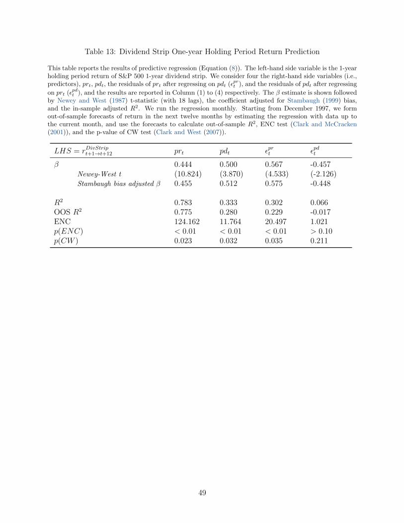
This simple model also shows that prt also predicts the expected return of one-year
dividend strip. Table 13 in the appendix shows that in-sample and out-of-sample R2 are
78.3% and 77.5% respectively. Specifically, we use prt to predict the return of buying an
one-year dividend strip and holding it until maturity. Such a high degree of predictability
strongly challenges the state-of-art structural asset pricing models.
2.5 Predicting return outside the United States.
Sample construction. The index return and futures data are obtained from Datastream.
Zero coupon bond yields and index dividends are obtained from Bloomberg. We start with
all developed countries with index futures, and drop a country from the sample if one of the
following criteria is met: 1) futures with maturity larger or equal to one year do not exist
(Germany, Hong Kong, Switzerland) or exist for less than five years (Norway); 2) futures
price exhibits strong seasonality (Italy, Netherlands, and Switzerland) or break (Canada).12
For each country, our sample starts from the earliest date when index return, futures, and
dividend data are all available. We end up with 1,469 country-month observations: UK
(FTSE100, starting in 1993), France (CAC40, starting in 1998), Spain (IBEX35, starting in
1994), Australia (ASX200, starting in 2002), and Japan (Nikkei225, starting in 1993). We
construct prt and pdt, and estimate εprt and εpdt country-by-country.
International return predictability. A potential concern is that our US sample of thirty
years (354 monthly observations) is relatively short. We supplements the US sample with
data from the other five countries, and use this unbalanced panel to test the return predictive
power of prt.
12In the appendix, Figure 11 plots the futures-to-spot ratio for these four countries.
19
Table 4: International Panel Return Prediction
This table reports the results of return forecasting regression (Equation (12)) using the panel data of Aus-tralia, France, Japan, Spain, the United Kingdom, and the United States. The left-hand side variable is theone-month, non-overlapping index return of a country, and for the right-hand side variable, we consider prt(Column 1 and 2), pdt (Column 3 and 4), εprt (Column 5 and 6), and εpdt (Column 7 and 8) in that country.
εprt is the residual of prt after regressing on pdt, and εpdt is the residual of pdt after regressing on prt. Foreach predictor, we report both the results with and without time fixed effects. The estimated predictivecoefficient (β) is shown followed by Hodrick (1992) t-statistic. In each column, we report whether countryand time fixed effects are included, the number of observations, and adjusted R2. We drop observations withnegative one-year dividend strip prices, so the estimation using prt has a shorter sample than that using pdt.
In the panel data regression, the left hand side variable is the future stock market return
in a country, and the right hand side variable of interest is prt in that country. Instead of
running the typical predictive regression with overlapping returns on the left hand side, we
follow the suggestion of Hodrick (1992) and run the following (“reverse”) regression to test
the return predictive power of prt at one-year horizon.
12 rnt,t+1 = α + β
(1
12
11∑i=0
xnt−i
)+ εnt,t+1, (12)
where n represents a country.13 The dependent variable is no longer overlapping. It is now
the (annualized) next-month market return, and the predictor, for example prt, is averaged
in the most recent twelve months. Hodrick (1992) points out the difficulties in inference when
using overlapping observations, especially the poor small-sample properties of GMM-based
autocovariances correction (e.g., Newey-West standard error), and suggest the regression in
13Note that the Hodrick (1992) standard error in Table 2 is not based on such non-overlapping regression.We corrected the standard error of predictive coefficient of overlapping regression following the calculationin Hodrick (1992) who show that under certain assumptions the corrected t-statistic of the overlappingregression equals the t-statistic of the non-overlapping reverse regression.
20
Equation (12) for drawing inference on long-run return prediction.14 We also cluster the
standard error by time and country. Therefore, the specification of Equation (12) combines
the better small-sample properties of Hodrick (1992) standard error and the advantage of
clustered standard errors in panel regression that are robust to cross-country and within-
country (time-series) correlation in the error term.
Table 4 reports the results. Column (1) shows the strong return predictive power of prt
after controlling for the heterogeneity in level of equity premium across countries (through
country fixed effect). The coefficient estimate is similar to the predictive coefficient in the
U.S. sample, and more statistically significant. The comparison between Column (1) and (3)
of Table 4 shows that the return predictive power of prt is stronger than pdt. Column (5)
shows that the residuals of prt after regressing on pdt strongly predicts return at one-year
horizon. Column (7) shows that prt largely subsumes the return predictive power of pdt (as
a reminder, εpdt is the residuals of pdt after regressing on prt), albeit that in comparison with
U.S. results, pdt seems to have some distinct information on future returns.
International comovement in the expected return. We introduce time fixed effect
in Column (2) that absorbs a global factor from realized returns of each country. Return
predictability disappears, meaning that the return predictive power of prt mainly comes from
the information it contains regarding the global factor that is common across countries. This
finding suggests that the variations of expected return across countries tend to comove, which
is in line with the literature of global equity market integration (Miranda-Agrippino and Rey
(2015)). And in Column (4), we see that any return predictive power of pdt also disappears
once the global factor is absorbed by the time fixed effect. Similar result holds in Column
(6) for the regression residuals of prt with respect to pdt.
Figure 10 in the Appendix shows the time series of the first three principal components
of prt in these countries, which together account for more than 80% of variation in prt.
The first principal component (48% of variation) exhibits spikes at the onsets of the global
financial crisis and the European sovereign debt crisis, suggesting that a major part of the
global comovement of expected stock return comes from crisis periods.
14Note that the adjusted R2 from the non-overlapping regression of Equation (12) is not comparable tothat of the overlapping regression in Table 2, because in Equation (12), we effectively forecast monthlyreturn using the one-year average of predictor, even if the inference we draw from such regression is aboutthe return prediction at one-year horizon. Thus, we do not report the R2 of non-overlapping regression.
21
US
UK
FR
A
ES
P
JP
N
AU
S0
5
10
15
20
25pr
pd
pr+pd
Figure 4: Return Prediction across Countries. This graph shows side-by-side the adjusted R2s of threeunivariate predictive regressions, with prt, pdt, and prt and pdt together on the right-hand side respectivelyfor each country. The left hand side variable is the total market return in the next twelve months.
Return predictability in each country. Figure 4 reports the adjusted R2 from predictive
regressions in each country using prt, pdt, and prt and pdt together on the right hand side.
prt outperforms pdt in all countries but Japan, and adding pdt does not seem to bring extra
return predictive power. Table 12 in the appendix reports the details of estimation results.
3 Asymmetric Predictability
In this section, we study conditional return predictability, and explore the economic mech-
anism behind predictability. We find that predictability is asymmetric – stronger following
a down market (Table 5). The results are similar outside the United States (Figure 5). We
evaluate the asset pricing models that imply strong asymmetry in return predictability by
using the proposed state variables as conditioning variables (Table 6).
22
3.1 Asymmetric return predictability: evidence
Conditional return prediction. We decompose prt into two components: (1) I(rt−12,t<0)×prt, the interaction between prt and an down-market indicator that equals one if the cumu-
lative market return in the past twelve months falls below the risk-free rate (i.e., the yield
of twelve-month zero-coupon bond); (2) I(rt−12,t≥0)× prt, the interaction between prt and the
up-market indicator.
rt,t+12 = α+βDI{rt−12,t<rft−12,t}
×prt+βUI{rt−12,t≥rft−12,t}×prt+βII{rt−12,t<r
ft−12,t}
+εt,t+12. (13)
Thus, the return predictive power of prt following a down market is reflected in βD, and the
return predictive power following an up market is reflect in βU .
Column (1) of Table 5 reports the regression results. Following a down market, prt
strongly predicts the market return at one-year horizon. The predictive power is much
weaker following an up market, i.e., when the market outperforms the risk-free benchmark.
In fact, βD is almost twice βU in both magnitude and the two t-statistics. The midpoint
between βD and βU is very close to the coefficient of prt as univariate predictor (Table
5). This decomposition by previous market condition reveals a sharp asymmetry in return
predictability.
Column (2) and (3) of Table 5 show that the down-market indicator itself does not
predict future returns or together with prt. When both the down-market indicator and prt
are used as predictors, the predictive coefficient on prt is almost identical to the predictive
coefficient in the univariate regression, and the t-statistics and R2s are almost identical.
Column (4) of Table 5 reports the results of an alternative specification,
rt,t+12 = α + βprt + ρ0
(rt−12,t − rft−12,t
)+ ρ1
(rt−12,t − rft−12,t
)× prt + εt,t+12. (14)
Adding the interaction term and the previous market excess return only changes the predic-
tive coefficient of prt by very little (in comparison with Table 2), but makes the coefficient
more statistically significant. Column (6) shows that adding the past market excess return
itself also does not change the predictive coefficient of prt by much, and the previous market
excess return does not forecast future return.
Time series momentum or reversal. The regression of Equation (14) shows that return
23
Table 5: Conditional Return Prediction
This table reports the results of conditional return prediction. The left-hand side variable of the regressionis the return of S&P 500 index in the next twelve months. We run the regression monthly. Column (1)reports the results of the specification of Equation (13). On the right-hand side are the interaction betweenprt and the down-market indicator (equal to one if the past twelve-month market return is below risk-freerate), the interaction between prt and the up-market indicator, the down-market indicator, and the intercept(omitted in table). Column (4) reports the results of the specification of Equation (14). On the right-handside are prt, the interaction between prt and the past twelve-month market excess return, the past-twelvemonth market excess return, and the intercept (omitted in table). The specifications of Column (2) and (5)has only the down-market indicator and the past twelve-month market excess return on the right-hand siderespectively. The specifications of Column (3) and (6) adds prt to Column (2) and (5) respectively. For eachspecification, the β estimate is shown followed by Newey and West (1987) and Hodrick (1992) t-statistics,and the adjusted R2 is reported in the last row.
autocorrelation is conditional on prt. This is related to papers on return autocorrelation
(Fama and French (1988); Poterba and Summers (1988)) that find positive return auto-
correlations at monthly and shorter horizons, and negative autocorrelations at annual and
longer horizons. But the evidence is not without debate (Kim, Nelson, and Startz (1991)).
Unconditional return autocorrelation is not significant at one-year horizon in Column
(5). But as suggested by Column (1) and (4) of Table 5, the relation between past and future
returns is a function of prt. As shown in Column (4), the return autocorrelation coefficient
is a function of prt, i.e., ρ0 + ρ1prt. With the mean of prt equal to 3.992 (Table 1), the
average of return autocorrelation coefficient is only 0.037. When prt is one-standard deviation
24
US UK FRA ESP JPN AUS−0.150
−0.125
−0.100
−0.075
−0.050
−0.025
0.000
0.025
Coefficients in up and down states
Up
Down
Figure 5: Conditional predictability across countries. Figure 5 reports the results of conditionalprediction (regression of Equation (13)) for different countries. The candle graph shows the estimates of βD(red) and βU (blue) together with the one Hodrick (1992) standard error band.
above its mean, the autocorrelation coefficient increases from 0.037 to 0.180, exhibiting
return momentum. When prt is one-standard deviation below its mean, the autocorrelation
coefficient is −0.106, exhibiting return reversal. While Campbell, Grossman, and Wang
(1993) find that daily return autocorrelation depends on trading volume, our results show
that at one year horizon, return autocorrelation is a function of the relative valuation of
long-term vs. short-term dividends.
Conditional predictability outside the United States. Figure 5 reports the results
of conditional prediction (regression of Equation (13)) for different countries. The candle
graph shows the estimates of βD (red) and βU (blue) together with the one Hodrick (1992)
standard error band. It is clear that except Japan, the return predictive power of prt is
more prominent following a down market. Table 12 in the appendix reports the details of
estimation results.
Our finding of asymmetric return predictability is related to the evidence on stronger
return predictive power of other variables (e.g., price-dividend ratio) during economic down-
turns.15 Henkel, Martin, and Nardari (2011) show that the return predictive power of price-
dividend ratio and short rate (Ang and Bekaert (2007)) appear non-existent during business
15Cujean and Hasler (2017) build an equilibrium model with counter-cyclical investors’ disagreement toexplain why stock return predictability is concentrated in bad times.
25
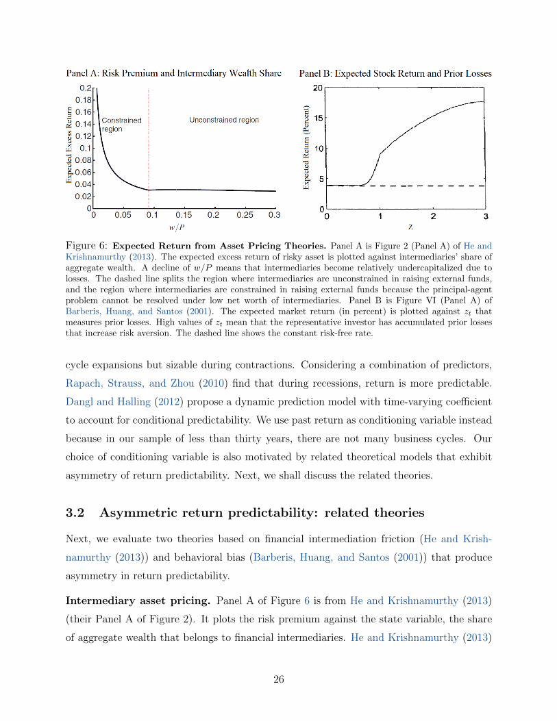
Figure 6: Expected Return from Asset Pricing Theories. Panel A is Figure 2 (Panel A) of He andKrishnamurthy (2013). The expected excess return of risky asset is plotted against intermediaries’ share ofaggregate wealth. A decline of w/P means that intermediaries become relatively undercapitalized due tolosses. The dashed line splits the region where intermediaries are unconstrained in raising external funds,and the region where intermediaries are constrained in raising external funds because the principal-agentproblem cannot be resolved under low net worth of intermediaries. Panel B is Figure VI (Panel A) ofBarberis, Huang, and Santos (2001). The expected market return (in percent) is plotted against zt thatmeasures prior losses. High values of zt mean that the representative investor has accumulated prior lossesthat increase risk aversion. The dashed line shows the constant risk-free rate.
cycle expansions but sizable during contractions. Considering a combination of predictors,
Rapach, Strauss, and Zhou (2010) find that during recessions, return is more predictable.
Dangl and Halling (2012) propose a dynamic prediction model with time-varying coefficient
to account for conditional predictability. We use past return as conditioning variable instead
because in our sample of less than thirty years, there are not many business cycles. Our
choice of conditioning variable is also motivated by related theoretical models that exhibit
asymmetry of return predictability. Next, we shall discuss the related theories.
3.2 Asymmetric return predictability: related theories
Next, we evaluate two theories based on financial intermediation friction (He and Krish-
namurthy (2013)) and behavioral bias (Barberis, Huang, and Santos (2001)) that produce
asymmetry in return predictability.
Intermediary asset pricing. Panel A of Figure 6 is from He and Krishnamurthy (2013)
(their Panel A of Figure 2). It plots the risk premium against the state variable, the share
of aggregate wealth that belongs to financial intermediaries. He and Krishnamurthy (2013)
26
model intermediaries as agents with exclusive access to risky assets. Intermediaries manage
wealth for the rest of economy (“households”), but the delegation capacity is linked to
intermediaries’ own wealth due to a typical principal-agent problem. When intermediaries
are relatively richer, their delegation capacity is sufficient to satisfy the needs of household,
and risk premium varies with the aggregate wealth of the economy, showing little variation
(“unconstrained region”). When intermediaries are relatively poor, the capacity constraint
binds, and the risk premium varies with the wealth of intermediaries, fluctuating widely. The
asymmetry of risk premium variation implies the asymmetry of return predictability. Our
down-market indicator, which spans a period of one year, is closely related to the observation
by Benartzi and Thaler (1995) that investors tend to evaluate fund performances annually
because they receive most comprehensive fund reports once a year.
Prospect theory. Panel B of Figure 6 is from Barberis, Huang, and Santos (2001). Their
model is built upon two ideas. First, investors are subject to loss aversion (Kahneman and
Tversky (1979)). Losses and gains from the stock market are defined with the risk-free
return as a benchmark. Second, how loss averse investors are, depends on their prior gains
and losses (Thaler and Johnson (1990)) against certain reference point. As they explain in
the paper: “after a prior gains, he becomes more less loss averse: the prior gains will cushion
any subsequent loss, making it more bearable. Conversely, after a prior loss, he becomes
more loss averse: after being burned by the initial loss, he is more sensitive to additional
setbacks.” Panel B of Figure 6 shows that the expected return barely moves when zt is below
one. zt measures the prior losses (if < 1) or gains (if > 1) against a historical benchmark.
Therefore, only under prior losses, the expected return exhibits large variation, which in turn
implies asymmetric return predictability.
Evaluation of related theories. Table 6 compares our results of conditional return pre-
diction with the results from empirical specifications suggested by the theories of He and
Krishnamurthy (2013) and Barberis, Huang, and Santos (2001). For each model, we con-
struct negative and positive indicator variable by comparing the value of conditioning vari-
able with a benchmark value, that is zero for our past excess return, average (i.e., η) for the
intermediary capital ratio of He, Kelly, and Manela (2017) (an empirical study of He and
Krishnamurthy (2013)), and one for zt of Barberis, Huang, and Santos (2001). Column (1)
and (4) repeat the results in Column (1) and (2) in Table 5.
27
Table 6: Evaluating Related Theories
This table reports the results of annual return prediction conditioning on three different variables: the pasttwelve-month market excess return, the intermediary net worth ηt in He, Kelly, and Manela (2017), andthe zt constructed following the model of Barberis, Huang, and Santos (2001). We construct negative andpositive indicator variables by comparing the three conditioning variable with zero, average, and one (assuggested by the theory) respectively. The specifications of Column (1) to (3) have the interaction termsbetween indicator variables and prt, the negative indicator variable, and the intercept (omitted in the table).The specifications of Column (4) to (6) have the negative indicator variables and the intercept (omitted inthe table). For each right-hand side variable, the coefficient estimate is shown followed by Newey and West(1987) and Hodrick (1992) t-statistics. For each specification, the adjusted R2 is reported in the last row.Note that we use ηt constructed by He, Kelly, and Manela (2017) whose sample ends in 2012.
rt−12,t − rft−12,t ηt − ηt z − 1 rt−12,t − rft−12,t ηt − ηt z − 1
Negative × prt -0.180 -0.247 -0.195Newey-West t (-3.810) (-2.340) (-5.221)Hodrick t [-2.977] [-2.101] [-2.990]
The empirical specifications suggested by both He and Krishnamurthy (2013) and
Barberis, Huang, and Santos (2001) produce results that are very similar to those of our
model with past excess return. The predictive coefficient on the interaction between negative
indicator and prt is twice as large as the coefficient on the interaction between positive
indicator and prt, and all three specifications in Column (1), (2), and (3) have adjusted R2
of similar magnitude. However, both theories predict that the conditioning variable itself
(captured by the negative indicator variable) should also predict returns, which is not the
case in data as shown by Column (5) and (6).
4 Variation in Expected Return
In this section, we use prt as forecasting variable to study the variation of expected return.
First, we show that expected return rises in response to monetary tightening, and it comoves
with variables that reflect conditions of macroeconomy and financial markets. Next, since
shocks to prt drives the variation of expected return, and thus, the investment opportunity
28
set, they should be priced in the cross-section of stocks by the logic of ICAPM. We find
a significant and negative price of prt risk. High pr-beta stocks, i.e., those that have high
realized returns when prt is high (the expected market return low), have low average returns.
4.1 Monetary policy and macroeconomy
The relation between macroeconomic conditions and the expected stock return has always
been at the center of asset pricing research (Fama and French (1989); Ferson and Harvey
(1991)). In particular, the impact of monetary policy on asset prices continues attracting
great attention (Campbell, Pflueger, and Viceira (2015))). Bernanke and Kuttner (2005)
find that an unanticipated cut in the Federal funds rate is associated with an increase in
stock indexes, and based on the VAR approach proposed by Campbell and Ammer (1993),
they show a largest part of stock price response is from changes in the expected return. More
recently, Lucca and Moench (2015) show that sizable fractions of realized stock returns are
concentrated in the twenty four hours before the scheduled meetings of the Federal Open
Market Committee (FOMC) in recent decades.
So far, we have shown that prt strongly predicts return at one-year horizon. Next, using
prt as a proxy of the expected return (or “discount rate”) in the stock market, we examine
how monetary policy affects stock prices through its impact on the discount rate and relate
our results to the existing literature. We also document significant correlations between the
expected returns from our predictive regression and various macroeconomic variables. Our
findings suggest that both monetary policy and business cycle fluctuations are important
drivers of the expected return in the stock market.
Monetary policy announcements and the expected return. To examine the impact
of monetary policy on stock prices, we construct four variables. We define a variable, FOMC
day, that equals one if the day has a FOMC meeting and zero otherwise. We also construct
a variable, Pre-FOMC day, that equals one if the next day has a FOMC meeting and zero
otherwise, and another variable, Post-FOMC day, that equals one if it is the previous day
has a FOMC meeting and zero otherwise. Finally, we use the monetary policy shocks from
Nakamura and Steinsson (2017) to construct a variable, MP Shock, that equals the value of
monetary policy shock on days of FOMC meetings and equals zero in non-FOMC days.16
16Monetary policy shock is calculated using a 30-minute window from 10 minutes before the FOMCannouncement to 20 minutes after it. Data of the Federal funds futures is used to separate changes in the
29
Table 7: Return, Expected Return, and Monetary Policy Announcements
This table reports how daily returns and expected returns (proxied by prt) changes during FOMC an-nouncement days and respond to monetary policy shocks. Monetary policy shock (MP Shock) is equal tothe unanticipated changes in the Federal Funds rate from Nakamura and Steinsson (2017) on the days ofFOMC meetings, and zero otherwise. “FOMC day” is the FOMC-day dummy variable. Pre-FOMC day isthe pre-FOMC day dummy variable. Post-FOMC day is the post-FOMC day dummy variable. The sampleperiod is 01 Jan 1988 to 31 Dec 2014 (the end of the sample of Nakamura and Steinsson (2017)). We regresscontemporaneous returns, pr, the residuals from regressing prt on pdt (i.e., εprt ), and the residuals from
regressing pdt on prt (i.e, εpdt ) on these monetary policy variables. The results are reported in each columnfor each specification. *, **, and *** denote 5%, 2%, and 1% level of statistical significance respectively.
Table 7 reports the results of regressing contemporaneous return, prt, pdt, the residuals
of pdt (w.r.t. prt), and the residuals of prt (w.r.t. pdt). Column (1) confirms the results of
Lucca and Moench (2015). The day of FOMC on average sees an average positive return
of 40 basis points. While Lucca and Moench (2015) argue that most of the realized market
returns are concentrated in the twenty four hours before FOMC announcements (on average
49 basis points per FOMC), a big fraction of the twenty four hours are on the FOMC day
because the time of the release usually varies between 12:30 pm and 2:30 pm. We do not
perform an intraday analysis because of the concern over intraday liquidity of S&P futures.
Column (2) of Table 7 shows a tightening of monetary policy (i.e., an increase in MP
Shock) leads to a decrease in stock market returns, in line with the evidence in Thorbecke
(1997) and Bernanke and Kuttner (2005). After controlling for the monetary policy shock
itself, the relation between stock return and FOMC day is weakened. It is a long tradition to
understand the contemporaneous response of stock price to monetary policy. Rozeff (1974)
finds that a substantial fraction of the variation in stock returns is related to contempora-
neous monetary developments.
target funds rate into anticipated and unanticipated components. For earlier contributions, please refer toCook and Hahn (1989), Kuttner (2001), and Cochrane and Piazzesi (2002) among others.
30
Our focus is on the regression of prt on the monetary policy variables, because prt
serves as a proxy for the expected stock return (i.e., the discount rate in the stock market).
Column (3) of Table 7 shows a negative response of prt to monetary tightening, which
translates into an increase in the expected return. In other words, unanticipated increase
in the Federal Funds rate tends to raise the expected stock return.17 Therefore, the decline
of stock price, i.e., the decrease of contemporaneous stock return, can be largely attributed
to the rising discount rate. Column (6) delivers the same message using the residuals of
prt from regressing prt on pdt. If we use the traditional price-dividend ratio as a proxy
for the expected return, we shall not see any response to monetary policy shock (as shown
in Column (4)) because the response of εprt to monetary policy shock is missed. Thus, our
new return predictor prt contains essential information about how the expected return varies
with monetary policy. Finally, since the residuals from regressing pdt on prt (i.e, εpdt ) strongly
forecast dividend growth (Table 3), we regress it on monetary policy variables. We do not
find significant relations.
In sum, monetary policy has strong impact on stock prices mainly through the discount
rate instead of cash flow growth – expansionary monetary policy tends to lower the discount
rate, and thereby, raise the stock price, leading to higher contemporaneous return. Since the
expected return is lower, the impact of monetary policy on stock price tends to revert in the
long run.
Correlation with other variables. The expected stock return is highly correlated with
variables that reflect the conditions of macroeconomy, financial markets, financial interme-
diaries, uncertainty, and sentiment (Table 8). Two versions of the expected returns are the
fitted values from unconditional (Equation (8)) and conditional (Equation (13)) predictive
regressions respectively. Both versions deliver a consistent message.
The expected return is countercyclical. It is positively correlated with unemployment,
and negatively correlated with consumption growth, fixed investments, and GDP deflector,
suggesting that a major fraction of variation in the expected return is from business cycle.
The expected return is also positively correlated with the term spread, and weakly correlated
with the default spread (Baa-Aaa) (Fama and French (1989)). The expected return comoves
with cay, as suggested by Lettau and Ludvigson (2001), but prt outperforms cay in return
17Our results are related to Patelis (1997) who documents some return predictive power of monetary policyvariables.
31
Table 8: Correlations between Macro Variables and the Expected Return
This table reports the correlation between the in-smaple fitted expected returns of unconditional and condi-tional models and macroecnomic variables. The variables are divided into four categories. 1) Macroeconomic:nominal GDP Growth, Industrial Production Growth (“IP Growth”), Chicago Fed National Activity Index(“CFNAI”), Unemployment Rate, Real Consumption Growth, Total Business Inventories, NonresidentialFixed Investment (nominal), Residential Fixed Investment (nominal), and GDP Deflator are all from FREDdatabase. 2) Financial: Term Spread and Default Spread (“Baa-Aaa”) are from FRED. cay is from Lettauand Ludvigson (2001). 3) Intermediary: Broker/Dealer leverage (“B/D Leverage”) is from Adrian, Etula,and Muir (2014); Broker/Dealer 1(5) year average CDS spreads (“B/D 1(5) Year Avg. CDS”) is fromGilchrist and Zakrajsek (2012); ROA of banks (“ROA Banks”) is from FRED. 4) Uncertainties: CBOE1-month VIX index (“VIX””) and Chauvet and Piger (2008)’s smoothed U.S. recession probabilities esti-mates for given month (“CP Recession”) are from FRED; Economics policy uncertainties (“EPU”) is fromBaker, Bloom, and Davis (2016); Survey of Professional Forecasters recession probability estimates (“SPFRecession”) is from the Philadelphia Fed. 5) Sentiments: Sentiment Index (both raw and orthogonalizedagainst several macro variables), Number of IPOs (“IPO #”) and close-end fund NAV discount (“Close-endDiscount”) are all from Baker and Wurgler (2006).
forecasting (Figure 3), especially out of sample. The fact that many of these cyclical variables
fail to predict return as strongly as prt does is likely because (1) we need better measurements
(e.g., see Savov (2011) for consumption), (2) most are only available at lower (quarterly)
frequencies, or (3) each of them reflects only a fraction of variation in the expected return
but prt is a comprehensive measure (sufficient statistics).18
The expected return exhibits strong negative correlation with broker-dealer leverage
(Adrian and Shin (2010); Tobias Adrian and Shin (2013)). This indicates that when dealer
banks increase their leverage to acquire risky assets or to extend credit to hedge funds through
prime brokerage services, the expected return tends to be low. The positive correlation
between the expected return and broker-dealer CDS spread suggests that the net worth
of financial intermediaries may also play a role in the variation of expected return (He and
Krishnamurthy (2013); He, Kelly, and Manela (2017)). We also find that the expected return
comoves with the profitability of commercial banks. Overall, the expected return is closely
associated with conditions of financial intermediation sector.
Interestingly, the expected return tends to be high when VIX is low. This finding
has important implications on the dynamics of risk-return trade-off (Lettau and Ludvigson
(2010)).19 Our finding is closely related to Moreira and Muir (2017), who show that a
trading strategy that scales up when the expected volatility declines tends to generate profits
unexplained by common risk factors.20 The expected return has a positive correlation with
policy uncertainty (EPU), but the correlations with recession probabilities are not conclusive.
Finally, we show that the expected return tends to be low when sentiment is high. The
sentiment index (raw and orthogonalized to macro factors) is from Baker and Wurgler (2006),
together with IPO volume and closed-end fund discount (inversely related to sentiment).
18For example, Lamont (2000) find that the aggregate nonresidual investment does not forecast returns.He suggests that investment plans are more responsive to variation in risk premia. In contrast, our measureof expected return is highly correlated with aggregate nonresidual investment, suggesting that the findingsof Lamont (2000) are likely to be biased by the noise between realized returns and expected returns. Pastorand Stambaugh (2009) propose a predictive system to address the imperfect correlation between expectedreturns and predictors.
19VIX may not capture the risk of change in investment opportunity set, which can be a importantcomponent of risk (Guo and Whitelaw (2006)).
20A similar risk-return trade-off manifests itself in the cross-section of stocks, as shown by the profitabilityof strategies that explore low-risk anomalies, such as idiosyncratic volatility (Ang et al. (2009)), risk parity(Asness, Frazzini, and Pedersen (2012)), and betting against beta (Frazzini and Pedersen (2014)).
33
4.2 pr risk price
Revisiting ICAPM. Investment opportunity set varies over time. Particularly, expected
stock market return varies with prt. Therefore, shocks to prt affects investors’ marginal value
of wealth and consumption through their impact on the investment opportunity.
When prt is high and the expected stock return is low, substitution effect suggests that
investors allocate more wealth to consumption rather than savings. Thus, positive pr shocks
lead to higher consumption and lower marginal utility of consumption and wealth. Assets
with high loadings on pr shocks (“high pr-beta”) pay off when wealth is less valued, so they
deliver a high average return in equilibrium. In other words, the price of pr risk is positive.
However, the deterioration of investment opportunity set (high prt) implies that in-
vestors become relatively poorer over time, so wealth effect suggests that investors consume
less in the current period. Thus, positive pr shocks lead to lower consumption and higher
marginal utility of consumption and wealth. High pr-beta assets pay off when additional
consumption is highly valued, so they deliver a low average return in equilibrium. The price
of pr risk is negative.
Whether substitution or wealth effect dominates, and whether consumption rises or
falls, depends on investors’ intertemporal elasticity of substitution. But either way, shocks
to prt affect consumption and the marginal value of wealth, so they should be priced in the
cross section of assets. Next, we estimate the price of pr risk in the cross-section of standard
sorted portfolios (i.e., size, value, momentum, investment, and profitability).
Any return predictor should go through this cross-section test. If predictive power is
not from spurious relations, shocks to the predictor are shocks to investment opportunity set,
and should be priced in the cross section. However, few studies on return predictors conduct
this economic test. In this paper, we go beyond statistical procedures, such as standard error
correction, bias adjustments, and out-of-sample test. By estimating the price of pr risk, we
test prt as a return predictor using the simple logic of ICAPM (Merton (1973)).
Estimating pr risk price. Our cross-section of assets are the twenty-five Fama-French
portfolios (sorted by market equity and book-to-market ratio), twenty-five momentum port-
folios (sorted by market equity and prior returns), twenty-five investment portfolios (sorted
by market equity and change in total assets), and twenty-five profitability portfolios (sorted
by market equity and operating profitability). The data of monthly portfolio returns are
34
from Kenneth R. French’s website.21 We consider this set of portfolios as good proxy for the
U.S. stock universe.
The first step is to calculate the loadings of assets on shocks to prt. As noted by Pastor
and Stambaugh (2003), an asset’s beta should be defined with respect to shocks (innovations)
instead of the level of a state variable, because expected changes in the state variable and
the expected asset return can be correlated, which contaminate beta measures. In our case,
prt is very likely to correlated with expected asset returns, because it forecasts market return
and expected asset returns are functions of expected market return by CAPM. We measure
shocks to prt as the first difference. In the appendix (Table 14), we show that results based
on AR(1) shocks are similar.
To estimate the price of pr shocks, we use two procedures. The first is the Fama-
MacBeth method. The second one is GMM, which corrects potential biases in Fama-
MacBeth standard errors (Cochrane (2005)). The parameters are over-identified. For the
weight matrix, we use the two-stage efficient weight matrix (Hayashi (2000)). In both cases,
the cross-sectional pricing equations exclude intercepts, and we include the market excess
return as the other risk factor following the equilibrium condition of ICAPM (Merton (1973)).
Table 9 reports the results of cross-sectional estimations. Each column corresponds to
a universe of assets. *, **, and *** denote 5%, 2%, and 1% level of statistical significance
respectively. “All” refers to the universe that includes Fama-French twenty-five portfolios,
ten momentum, ten investment, and ten profitability portfolios (a total of fifty-five assets).
Column (2) to (5) correspond respectively to twenty-five double sorted portfolios of book-
to-market, momentum, investment and profitability with size. The price of risk is reported
for both pr shock (∆prt) and market excess return (rt − rft ), followed by the t-statistic. We
also report the mean absolute pricing error (MAPE) and R2.
The price of pr risk is negative and statistically significant in the cross-section of all
assets, size and book-to-market sorted portfolios, momentum portfolios, and profitability
portfolios. The magnitude is similar across asset universes, and economically significant.
For example, one standard deviation difference in the pr beta of two assets corresponds to a
difference of 0.252 × 0.00685 × 12 = 2.1% in average return per annum. A significant price
of pr risk helps establish prt as a return predictor or proxy for expected market return.
Among size (SMB), value (HML), profitability (RMW), investment (CMA) and mo-
This table reports the price of market risk and pr risk estimated using Fama-MacBeth method and Gen-eralized Method of Moments (GMM). We use the two-stage GMM estimator with efficient weight matrix.prt shock is measured by the firs difference of prt. The full asset universe (“All”) includes the twenty fiveFama-French portfolios (sorted by size and book-to-market ratio), ten momentum portfolios, ten invest-ment portfolios, and ten profitability portfolios. We also estimate pr risk price using twenty five value-size,momentum-size, investment-size, and profitability-size portfolios. The data of monthly portfolio returns arefrom Kenneth R. French’s website. Each column corresponds to one set of assets. Each estimated price ofrisk is follwed by the t-statistic in parenthesis. *, **, and *** denote 5%, 2%, and 1% level of statisticalsignificance respectively. We also report mean absolute pricing error (MAPE) and R2.
Figure 7: Out-of-sample R2 by Sample Split Date.This graph reports out-of-sample R2 with differentsample split dates of 1-year return prediction. The first and last out-of-sample split date are Jan 1993 andJun 2012 respectively.
pin down the constant A = 1 and obtain
s1 =
√s20 +R2
1−R2. (15)
Appendix II: Additional Results
II.1 Alternative out-of-sample sample splits
In the main text, we report out-of-sample forecasting tests based on a 1988 sample split
date, but recent forecast literature suggests that sample splits themselves can be data-mined
(see Hansen and Timmermann (2012) and Rossi and Inoue (2012)). To demonstrate the
robustness of out-of-sample forecasts to alternative sample splits, Figure 7 plots out-of-
sample annual return predictive R2 as a function of the sample split for a variety of predictors.
We consider a sample split as early as 1993. The latest split we consider is Jun 2012 (5-year
prior to the end of our sample), which uses a 24.5-year training sample.
For early sample splits, for example 1994, the training (i.e., estimation) sample is
relatively short, so the precision of coefficient estimate is poor, which contributes to the
40
Table 10: One-month Return Prediction
This table reports the results of predictive regression (Equation (8)). The left-hand side variable is the returnof S&P 500 index in the next month. We consider four the right-hand side variables (i.e., predictors), prt,
pdt, the residuals of prt after regressing on pdt (εprt ), and the residuals of pdt after regressing on prt (εpdt ),and the results are reported in Column (1) to (4) respectively. The β estimate is shown followed by Hodrick(1992) t-statistic and the in-s1ample adjusted R2. We run the regression monthly. Starting from December1997, we form out-of-sample forecasts of return in the next month by estimating the regression with dataonly up to the current month, and use the forecasts to calculate out-of-sample R2. ENC statistic (Clark andMcCracken (2001)), and the p-value of CW statistic (Clark and West (2007)).
prt pdt εprt εpdt
β -0.010 -0.015 -0.011 0.004Hodrick t [-2.197] [-2.006] [-0.959] [0.215]
low out-of-sample R2 that we see in the early years. As the sample split date progresses,
the estimation sample extends, and the evaluation sample starts to exclude more data from
earlier dates in the calculation of out-of-sample R2. Excluding the dotcom burst, i.e. out-
of-sample split starting 2002 or later, leads to a relatively low R2 for both prt and pdt,
suggesting that both predictors perform well during the dotcom burst. Using data starting
from the 2007-09 crisis, pdt delivers a higher out-of-sample R2 than prt. The reason is that its
denominator, i.e., the rolling sum of dividends, reacts to the crisis sluggishly, so the decrease
of pdt is larger than the decrease of prt throughout the crisis, coinciding with the slump of
market return. After the financial crisis, prt outperforms pdt out-of-sample.
II.2 Monthly return prediction
One-month return prediction. Table 10 reports the results of one-month return predic-
tion. The predictive coefficient is large in magnitude and statistically significant. A decrease
of prt by one standard deviation adds 0.53% to the expected monthly return (annualized to
6.55%). The out-of-sample R2 of 0.9% implies a large improvement in investment perfor-
mance for an investor who rebalances portfolio monthly and uses prt to time the market. For
a mean-variance investor, Campbell and Thompson (2008) show that in comparison with a
41
buy-and-hold strategy, the proportional increase in the expected return from observing prt
is(
R2
1−R2
)(1+S2
S2
), where R2 is the out-of-sample R2 and S2 is the squared Sharpe ratio of
stock returns. Given the monthly Sharpe ratio of 0.1570 (annualized to 0.544), a monthly
out-of-sample R2 of 0.9% implies a 36.5% proportional improvement of expected return.
The difference in return predictive power between pdt and prt is smaller at one-month
forecasting horizon than at one-year horizon. pdt has an out-of-sample R2 of 0.7% (Column
(2) of Table 10), and the residual of prt after regressing on pdt does not significantly forecast
monthly return. This suggests that the additional return predictive power of prt beyond pdt
is mainly at longer horizons.
42
II.3 Additional figures
1997 1999 2001 2003 2005 2007 20093.5
4.0
4.5
5.0
5.5
6.0
6.5
correlation = 0.88
prt constructed using futures and options
prt futures
prt options
Figure 8: prt from Futures and Option Data. This graph reports prt constructed from futures andoption data (from Binsbergen, Brandt, and Koijen (2012) from January 1996 and October 2009).
43
19941998
20022006
20102014
Date
−3
−2
−1
0
1
2
3βpr
βpd
Figure 9: Predictive Coefficient Stability. This graph plots the predictive coefficient (and its 95%confidence band in shade) estimated using one-year rolling window of daily observations. The first rollingwindow ends in December 1988.
44
20042006
20082010
20122014
−2
−1
0
1
2
3
4
5
6Principle Components of prt across countries
PC1, 48.00%
PC2, 33.17%
PC3, 16.16%
Figure 10: Principal Components of prt. This figure plots the first three principal components of prtin US, UK, France, Spain, Japan and Australia.
Figure 11: Futures-to-spot ratio of international stock indices. This graph plots 1-year futures-to-spot ratio of international stock indices. There are 4 countries, Canada, Italy, Netherlands, and Switzerland.
46
II.4 Additional tables
Table 11: Correlations with other common return predictors
This table shows the correlation of alternative return predictors with both prt and pdt from 1988 to 2016.Most alternative predictors are from Goyal and Welch (2007) that include the default yield spread (dfy),the inflation rate (infl), stock variance (svar), the cross-section premium (csp), the dividend payout ratio(de), the long-term yield (lty), the term spread (tms), the T-bill rate (tbl), the default return spread (dfr),the dividend yield (dy, log difference between current-period dividend and lagged S&P 500 index price),the long-term rate of return (ltr), the earnings-to-price ratio (ep), the book to market ratio (bm), theinvestment-to-capital ratio (ik), the net equity expansion ratio (ntis), the percent equity issuing ratio (eqis),and the consumption-wealth-income ratio (cay). Liquidity is the liquidity factor from Pastor and Stambaugh(2003). SII is the short interests index from Rapach, Ringgenberg, and Zhou (2016) (1988-2014). SVIX isoption-implied lower bound of 1-year equity premium from Martin (2017) (1996-2012). ZCB1Y is 1-yearzero coupon bond yield from Fama-Bliss.
Table 12: Country-by-country unconditional and conditional return predictions
This table reports the results of international country-by-country return predictions for US, UK, France,Spain, Japan and Australia. Panel A and B tabulate the results of unconditional (Equation (8)) andconditional (Equation (13)) return predictions respectively for each country. The coefficients estimates arefollowed by Newey and West (1987) t-statistic (with 18 lags) and Hodrick (1992) t-statistic. Interceptestimates are untabulated.
Table 13: Dividend Strip One-year Holding Period Return Prediction
This table reports the results of predictive regression (Equation (8)). The left-hand side variable is the 1-yearholding period return of S&P 500 1-year dividend strip. We consider four the right-hand side variables (i.e.,predictors), prt, pdt, the residuals of prt after regressing on pdt (εprt ), and the residuals of pdt after regressing
on prt (εpdt ), and the results are reported in Column (1) to (4) respectively. The β estimate is shown followedby Newey and West (1987) t-statistic (with 18 lags), the coefficient adjusted for Stambaugh (1999) bias,and the in-sample adjusted R2. We run the regression monthly. Starting from December 1997, we formout-of-sample forecasts of return in the next twelve months by estimating the regression with data up tothe current month, and use the forecasts to calculate out-of-sample R2, ENC test (Clark and McCracken(2001)), and the p-value of CW test (Clark and West (2007)).
This table reports the price of market risk and pr risk estimated using Fama-MacBeth method and Gener-alized Method of Moments (GMM). We use the two-stage GMM estimator with efficient weight matrix. prtshock is measured by AR(1) residual (εprt ) estimated using the full sample. The full asset universe (“All”)includes the twenty five Fama-French portfolios (sorted by size and book-to-market ratio), ten momentumportfolios, ten investment portfolios, and ten profitability portfolios. We also estimate pr risk price usingtwenty five value-size, momentum-size, investment-size, and profitability-size portfolios. The data of monthlyportfolio returns are from Kenneth R. French’s website. Each column corresponds to one set of assets. Eachestimated price of risk is follwed by the t-statistic in parenthesis. *, **, and *** denote 5%, 2%, and 1%level of statistical significance respectively. We also report mean absolute percentage error (MAPE) and R2.
Table 15: Correlation Between pr shocks and U.S. Stock Market Factors
This table documents the correlation between prt shocks and market excess return, size factor (SMB), valuefactor (HML), profitability factor (RMW), investment factor (CMA), and momentum factor. The factorreturns are obtain from Kenneth R. French’s website. We consider two versions of prt shocks, the firstdifference (∆prt ) and AR(1) residual (εprt ) estimated using full sample.
Adrian, T., E. Etula, and T. Muir (2014). Financial Intermediaries and the Cross-Sectionof Asset Returns. Journal of Finance LXIX (6), 1–56.
Adrian, T. and H. S. Shin (2010). Liquidity and leverage. Journal of Financial Intermedia-tion 19 (3), 418 – 437. Risk Transfer Mechanisms and Financial Stability.
Ang, A. and G. Bekaert (2007). Stock return predictability: Is it there? The Review ofFinancial Studies 20 (3), 651–707.
Ang, A., R. J. Hodrick, Y. Xing, and X. Zhang (2009). High idiosyncratic volatility and lowreturns: International and further u.s. evidence. Journal of Financial Economics 91 (1),1 – 23.
Asness, C. S., A. Frazzini, and L. H. Pedersen (2012). Leverage aversion and risk parity.Financial Analysts Journal 68 (1), 47–59.
Baker, M. and J. Wurgler (2006). Investor sentiment and the cross-section of stock returns.Journal of Finance LXI (4), 1645–1680.
Baker, S. R., N. Bloom, and S. J. Davis (2016). Measuring Economic Policy Uncertainty.The Quarterly Journal of Economics 131 (4), 1593–1636.
Ball, R. and R. Watts (1972). Some time series properties of accounting income. The Journalof Finance 27 (3), 663–681.
Bansal, R. and A. Yaron (2004). Risks for the long run: A potential resolution of assetpricing puzzles. The Journal of Finance 59 (4), 1481–1509.
Barberis, N., M. Huang, and T. Santos (2001). Prospect theory and asset prices. TheQuarterly Journal of Economics 116 (1), 1–53.
Benartzi, S. and R. H. Thaler (1995). Myopic loss aversion and the equity premium puzzle.The Quarterly Journal of Economics 110 (1), 73–92.
Bernanke, B. S. and K. N. Kuttner (2005). What explains the stock market’s reaction tofederal reserve policy? The Journal of Finance 60 (3), 1221–1257.
Binsbergen, J. H. V., M. W. Brandt, and R. S. J. Koijen (2012, jun). On the Timing andPricing of Dividends. American Economic Review 102 (4), 1596–1618.
Binsbergen, J. H. V., W. Hueskes, R. S. J. Koijen, and E. B. Vrugt (2013, dec). Equityyields. Journal of Financial Economics 110 (3), 503–519.
Binsbergen, J. H. V. and R. S. J. Koijen (2010). Predictive Regressions: A Present-ValueApproach. Journal of Finance LXV (4), 1439–1471.
Binsbergen, J. H. V. and R. S. J. Koijen (2017). The term structure of returns: Facts andtheory. Journal of Financial Economics 124 (1), 1 – 21.
52
Bossaerts, P. and P. Hillion (1999). Implementing Statistical Criteria to Select ReturnForecasting Models: What Do We Learn? . Review of Financial Studies 12 (2), 405–428.
Campbell, J. Y. and J. Ammer (1993). What moves the stock and bond markets? a variancedecomposition for long-term asset returns. The Journal of Finance 48 (1), 3–37.
Campbell, J. Y. and J. H. Cochrane (1999). By force of habit: A consumptionbased expla-nation of aggregate stock market behavior. Journal of Political Economy 107 (2), 205–251.
Campbell, J. Y., S. J. Grossman, and J. Wang (1993). Trading volume and serial correlationin stock returns*. The Quarterly Journal of Economics 108 (4), 905–939.
Campbell, J. Y., C. Pflueger, and L. M. Viceira (2015). Monetary policy drivers of bondand equity risks. Working paper, Harvard University.
Campbell, J. Y. and R. J. Shiller (1988). The Dividend-Price Ratio and Expectations ofFuture Dividends and Discount Factors. Review of Financial Studies 1 (3), 195–228.
Campbell, J. Y. and S. B. Thompson (2008). Predicting excess stock returns out of sample:Can anything beat the historical average? The Review of Financial Studies 21 (4), 1509–1531.
Chauvet, M. and J. Piger (2008). A comparison of the real-time performance of businesscycle dating methods. Journal of Business and Economic Statistics 26, 4249.
Clark, T. E. and M. W. McCracken (2001). Tests of equal forecast accuracy and encom-passing for nested models. Journal of Econometrics 105 (1), 85 – 110. Forecasting andempirical methods in finance and macroeconomics.
Clark, T. E. and K. D. West (2007). Approximately normal tests for equal predictive ac-curacy in nested models. Journal of Econometrics 138 (1), 291 – 311. 50th AnniversaryEconometric Institute.
Cochrane, J. H. (1991). Production-based asset pricing and the link between stock returnsand economic fluctuations. The Journal of Finance 46 (1), 209–237.
Cochrane, J. H. (1992). Explaining the variance of pricedividend ratios. Review of FinancialStudies 5 (2), 243–280.
Cochrane, J. H. (2005). Asset Pricing (Revised Edition ed.). Princeton, NJ: PrincetonUniversity Press.
Cochrane, J. H. (2007, mar). The Dog That Did Not Bark: A Defense of Return Predictabil-ity. Review of Financial Studies 21 (4), 1533–1575.
Cochrane, J. H. (2008). State-space vs. var models for stock returns. Unpublished paper,Chicago GSB .
Cochrane, J. H. and M. Piazzesi (2002, May). The fed and interest rates - a high-frequencyidentification. American Economic Review 92 (2), 90–95.
53
Cook, T. and T. Hahn (1989). The effect of changes in the federal funds rate target onmarket interest rates in the 1970s. Journal of Monetary Economics 24 (3), 331–351.
Cujean, J. and M. Hasler (2017). Why does return predictability concentrate in bad times?The Journal of Finance, forthcoming.
Da, Z., R. Jagannathan, and J. Shen (2014, October). Growth expectations, dividend yields,and future stock returns. Working Paper 20651, National Bureau of Economic Research.
Dangl, T. and M. Halling (2012). Predictive regressions with time-varying coefficients. Jour-nal of Financial Economics 106 (1), 157 – 181.
Duffie, D. (2001). Dynamic Asset Pricing Theory (3 ed.). Princeton Series in Finance.Princeton, N.J.: Princeton University Press.
Fama, E. and K. French (2000). Forecasting profitability and earnings. The Journal ofBusiness 73 (2), 161–75.
Fama, E. F. and K. R. French (1988). Permanent and temporary components of stock prices.Journal of Political Economy 96, 246–273.
Fama, E. F. and K. R. French (1989). Business conditions and expected returns on stocksand bonds. Journal of Financial Economics 25 (1), 23 – 49.
Ferson, W. and C. Harvey (1991). The variation of economic risk premiums. Journal ofPolitical Economy 99 (2), 385–415.
Ferson, W. E., S. Sarkissian, and T. T. Simin (2003). Spurious regressions in financialeconomics? The Journal of Finance 58 (4), 1393–1413.
Foster, F. D., T. Smith, and R. E. Whaley (1997). Assessing goodness-of-fit of asset pricingmodels: The distribution of the maximal r¡sup¿2¡/sup¿. The Journal of Finance 52 (2),591–607.
Frazzini, A. and L. H. Pedersen (2014). Betting against beta. Journal of Financial Eco-nomics 111 (1), 1 – 25.
Gilchrist, S. and E. Zakrajsek (2012, June). Credit spreads and business cycle fluctuations.American Economic Review 102 (4), 1692–1720.
Golez, B. (2014). Expected returns and dividend growth rates implied by derivative markets.The Review of Financial Studies 27 (3), 790–822.
Gordon, M. J. (1962). The Investment, Financing, and Valuation of the Corporation. Irwinseries in economics. Homewood, IL: R.D. Irwin.
Goyal, A. and I. Welch (2007, mar). A Comprehensive Look at The Empirical Performanceof Equity Premium Prediction. Review of Financial Studies 21 (4), 1455–1508.
54
Guo, H. and R. F. Whitelaw (2006). Uncovering the riskreturn relation in the stock market.The Journal of Finance 61 (3), 1433–1463.
Hansen, P. R. and A. Timmermann (2012). Choice of sample split in out-of-sample forecastevaluation. Working paper, Stanford University.
Hayashi, F. (2000). Econometrics. Princeton, NJ: Princeton University Press.
He, Z., B. Kelly, and A. Manela (2017). Intermediary asset pricing: New evidence frommany asset classes. Journal of Financial Economics .
He, Z. and A. Krishnamurthy (2013). Intermediary asset pricing. American EconomicReview 103 (2), 732–70.
Henkel, S. J., J. S. Martin, and F. Nardari (2011). Time-varying short-horizon predictability.Journal of Financial Economics 99 (3), 560 – 580.
Hodrick, R. J. (1992). Dividend Yields and Expected Stock Returns: Alternative Proceduresfor Inference and Measurement. Review of Economic Dynamics 5 (3), 357–386.
Kahneman, D. and A. Tversky (1979). Prospect theory: An analysis of decision under risk.Econometrica 47 (2), 263–291.
Kelly, B. and S. Pruitt (2013). Market Expectations in the Cross-Section of Present Values.Journal of Finance LXVIII (5), 1721–1756.
Kim, M. J., C. R. Nelson, and R. Startz (1991). Mean reversion in stock prices? a reappraisalof the empirical evidence. The Review of Economic Studies 58 (3), 515–528.
Koijen, R. S. J. and S. van Nieuwerburgh (2011). Predictability of Returns and Cash Flows.Annual Review of Financial Economics 3, 467–491.
Kuttner, K. (2001). Monetary policy surprises and interest rates: Evidence from the fedfunds futures market. Journal of Monetary Economics 47 (3), 523–544.
Lacerda, F. and P. Santa-Clara (2010). Forecasting dividend growth to better predict returns.Working paper, Universidade Nova de Lisboa.
Lamont, O. A. (2000). Investment plans and stock returns. The Journal of Finance 55 (6),2719–2745.
Lettau, M. and S. Ludvigson (2001). Consumption, aggregate wealth, and expected stockreturns. The Journal of Finance 56 (3), 815–849.
Lettau, M. and S. C. Ludvigson (2005). Expected returns and expected dividend growth.Journal of Financial Economics 76 (3), 583 – 626.
Lettau, M. and S. C. Ludvigson (2010). {CHAPTER} 11 - measuring and modeling variationin the risk-return trade-off. In Y. AT-SAHALIA and L. P. HANSEN (Eds.), Handbook ofFinancial Econometrics: Tools and Techniques, Volume 1 of Handbooks in Finance, pp.617 – 690. San Diego: North-Holland.
55
Lucca, D. O. and E. Moench (2015). The pre-fomc announcement drift. The Journal ofFinance 70 (1), 329–371.
Martin, I. (2017). What is the expected return on the market?*. The Quarterly Journal ofEconomics 132 (1), 367–433.
Menzly, L., T. Santos, and P. Veronesi (2004). Understanding predictability. Journal ofPolitical Economy 112 (1), 1–47.
Merton, R. C. (1973). An intertemporal capital asset pricing model. Econometrica 41 (5),867–887.
Miranda-Agrippino, S. and H. Rey (2015, November). World asset markets and the globalfinancial cycle. Working Paper 21722, National Bureau of Economic Research.
Moreira, A. and T. Muir (2017). Volatility-managed portfolios. The Journal of Fi-nance 72 (4), 1611–1644.
Muir, T. (2017). Financial crises and risk premia. The Quarterly Journal of Eco-nomics 132 (2), 765–809.
Nakamura, E. and J. Steinsson (2017). High frequency identification of monetary non-neutrality: The information effect. Quarterly Journal of Economics , forthcoming.
Nelson, C. R. and M. J. Kim (1993). Predictable stock returns: The role of small samplebias. The Journal of Finance 48 (2), 641–661.
Newey, W. K. and K. D. West (1987). A simple, positive semi-definite, heteroskedasticityand autocorrelation consistent covariance matrix. Econometrica 55 (3), 703–708.
Pastor, L. and R. F. Stambaugh (2009). Predictive systems: Living with imperfect predictors.The Journal of Finance 64 (4), 1583–1628.
Pastor, u. and R. F. Stambaugh (2003). Liquidity Risk and Expected Stock Returns. Journalof Political Economy 111 (3), 642–685.
Patelis, A. D. (1997). Stock return predictability and the role of monetary policy. TheJournal of Finance 52 (5), 1951–1972.
Poterba, J. M. and L. H. Summers (1988). Mean reversion in stock prices: Evidence andimplications. Journal of Financial Economics 22 (1), 27 – 59.
Presidential Task Force on Market Mechanisms (Chairman: Nicholas Brady) (1988). Reportof the Presidential Task Force on Market Mechanisms: submitted to The President of theUnited States, The Secretary of the Treasury, and The Chairman of the Federal ReserveBoard. Washington, D.C.: U.S. Government Printing Office.
Rapach, D. E., M. C. Ringgenberg, and G. Zhou (2016). Short interest and aggregate stockreturns. Journal of Financial Economics 121 (1), 46 – 65.
56
Rapach, D. E., J. K. Strauss, and G. Zhou (2010). Out-of-sample equity premium pre-diction: Combination forecasts and links to the real economy. The Review of FinancialStudies 23 (2), 821–862.
Rossi, B. and A. Inoue (2012). Out-of-sample forecast tests robust to the choice of windowsize. Journal of Business & Economic Statistics 30 (3), 432–453.
Rozeff, M. S. (1974). Money and stock prices: Market efficiency and the lag in effect ofmonetary policy. Journal of Financial Economics 1 (3), 245–302.
Rytchkov, O. (2012). Filtering out expected dividends and expected returns. QuarterlyJournal of Finance 02 (03), 1250012.
Savov, A. (2011). Asset pricing with garbage. The Journal of Finance 66 (1), 177–201.
Stambaugh, R. F. (1999). Predictive Regressions. Journal of Financial Economics 54, 375–421.
Thaler, R. H. and E. J. Johnson (1990). Gambling with the house money and trying tobreak even: The effects of prior outcomes on risky choice. Management Science 36 (6),643–660.
Thorbecke, W. (1997). On stock market returns and monetary policy. The Journal ofFinance 52 (2), 635–654.
Tobias Adrian, E. M. and H. S. Shin (2013). Dynamic leverage asset pricing. Working Paper625, Federal Reserve Bank of New York.