Reduced-complexity Noncoherent Receiver for GMSK … Equalization for Noncoherent Systems 20 3...

$Page 1: Reduced-complexity Noncoherent Receiver for GMSK … Equalization for Noncoherent Systems 20 3 Demodulating GMSK with Adaptive DFE in AWGN Channel 24 3.1 The Laurent .\ pproximation$
Reduced-complexity Noncoherent

Receiver for GMSK Signals

Houhao Wang

-4 thesis submitted in conformity with the requirements

for the degree of Master of Applied Science

Graduate Department of Electrical and Computer Engineering

University of Toronto

@Copyright by Houhao Wang 2001

National Library 191 of Canada Bibliothèque nationale du Canada

Acquisitions and Acquisitions et Bi bliog raphic Services services bibliographiques

395 WeUington Street 395. rue Wellington OnawaON K l A O W Ottawa ON K l A ON4 Carmda Canada

The author has granted a non- exclusive licence allowing the National Library of Canada to reproduce, loan, distribute or seli copies of this thesis in microfom, paper or electronic formats.

The author retains ownership of the copyright in this thesis. Neither the thesis nor substantial extracts fkom it may be printed or otherwise reproduced without the author's permission.

L'auteur a accordé une licence non exclusive permettant à la Bibliothèque nationale du Canada de reproduire, prêter, distribuer ou vendre des copies de cette thèse sous la forme de microfiche/film, de reproduction sur papier ou sur format électronique.

L'auteur consme la propriété du droit d'auteur qui protège cette thèse. Ni la thèse ni des extraits substantiels de celle-ci ne doivent être imprimés ou autrement reproduits sans son autorisation.

Reduced-complexity Noncoherent Receiver for

GMSK Signais

Houhao Wang

A thesis submitted in conformity with the requirements for the Degree of Master of

Applied Science, Graduate Department of Electrical and Cornputer Engineering, i n

the University of Toronto, 2001

Abstract

Gaussian Minimum Shift Keying(GhlS1i) is a spectrum and power efficient mod-

ulation scheme, used in many wireless communication systems. Since GMSK is nori-

linear, the rcceiver for GMSK signals is more complex than that for linear modulation

signals. -4 reduction in complexity can be achieved by employing a noncoherent signal

detectioii scheme.

In this thesis, a reduced complexity noncoherent GMSK receiver, using the Lau-

rent representation and noncoherent Decision Feedback Equalization(DFE), is pro-

posed and evaluated first in an Additive White Gaussian Noise(AMTGN) channel. The

Bit Error Rate(BER) performance of the proposed receiver is compared t o a corre-

sponding coherent receiver. Furthermore, the proposed receiver is evaluated in static

Finite Impulse Response(F1R) channels and multipath Rayleigh fading channels. The

effects of two intrinsic parameters on performance are examined. It is concluded that

the proposed receiver is a high performance noncoherent receiver when compared to

other known noncoherent GMSK receivers.

Acknowledgement s

1 am deeply gratefuI to my supervisor, Prof. S. Pasupathy, for his guidance and

support throughout the course of my graduate studies. His numerous comments and

careful reading of the manuscript are greatly appreciated.

1 would Iike to thank Dr. R. Schober for his help and prompt replies to my

questions.

1 gratefully acknowledge the financial support I received in the form of the Ontario

Graduate Scholarship, the University of Toronto Open Masters Fellowship and the

research assistantsliip provided by Prof. S. Pasupathy.

Finally, 1 would like to thank my family for their patience, support and encour-

agement.

Contents

List of Figures v

List of Tables viii

List of Acronyms x

1 Introduction 1

1.1 Motivation . . . . . . . . . . . . . . . . . . . . . . . . . . . . . . . . . 1

. . . . . . . . . . . . . . . . . . . . . . . . . . 1.2 Organization of Thesis 3

Background and Literature Survey 4

. . . . . . . . . . . . . . . . . 2.1 GMSK and the Laurent Representation 4

. . . . . . . . . . . . . . . . . . . . . . . . . . . . . . . 2.1.1 GACISI< 4

2.1.2 The Laurent Representation of CPM . . . . . . . . . . . . . . 7

. . . . . . . . . . . . . . . . . . . . . . . . . . . . . . 2.9 Signal Detection 10

. . . . . . . . . . . . . . . . . . . . . . . . 2.3 Multipath Fading Channel 11

. . . . . . . . . . . . . . . . . . . 2.4 Equalizatioii for -4 Coherent System 13

. . . . . . . . . . . 2.4.1 Maximum Likelihood Sequence Estimation 13

. . . . . . . . . . . . . . . . . 2.42 Linear Transversal Equalization 14

. . . . . . . . . . . . . . . . . 2.4.3 Decision Feedback Equalization 15

. . . . . . . . . . . . . . . . . . . . . . 2.4.4 Adaptive Equalization 17

. . . . . . . . . . . . . . . . 2 . 4 5 Fractionally Spaced Equalization 18

iii

. . . . . . . . . . . . . . . . . 2.5 Equalization for Noncoherent Systems 20

3 Demodulating GMSK with Adaptive DFE in AWGN Channel 24

3.1 The Laurent .\ pproximation of GMSK Signals . . . . . . . . . . . . . 25

3.1.1 .A pprosimating GMSK as Binary Difierential PSK . . . . . . . 27

3.2 Detecting GMSK with -4 Coherent -4daptive DFE . . . . . . . . . . . 29

. . . . . . . . . . . . . 3.3.1 Coherent GMSK Receiver Performance 32

. . . . . . . . . . . . . . . . . . . . . . . . 3.2.2 Simulating GMSK 32

3.2.3 Sensitivity to Frequency Offset . . . . . . . . . . . . . . . . . 33

3.3 Differential Detection of GMSK signals with -4daptive NDFE . . . . . 35

. . . . . . . . . . . . . . . . . . . . 3.3.1 Schober's-4daptiveRY:DFE 36

3.3.3 Noncoherent GMSK Receiver Performance . . . . . . . . . . . 41

. . . . . . . . . . . . . . . . . 3.3.3 Sensitivity to Frequency Offset 43

. . . . . . . . . . . . . . . . . . . . . . . . . . 3.3.4 The Role of BT 44

. . . . . . . . . . . . . . . . . . . . 3.3.5 Fractionally Spaced NDFE 47

3.3.6 Performance Versus Other Noncoberent GMSK Receivers . . . 47

4 Reduced-complexity Noncoherent Receiver in Fading Channels 50

. . . . . . . . . . . . . . . . . . . 4.1 Performance Under Static ChanneIs 51

. . . . . . . . . . . . . . . . . . . . . . . . . . 4.1.1 StaticChannels 51

4.1.2 Simulation Results . . . . . . . . . . . . . . . . . . . . . . . . 53

4.2 Performance Under Rayleigh Fading Channels . . . . . . . . . . . . . 54

4.2.1 Rayleigh Fading Channel Mode1 . . . . . . . . . . . . . . . . . 54

4.2.2 Simulation Results . . . . . . . . . . . . . . . . . . . . . . . . 57

5 Conclusion 60

1 Summary of Results . . . . . . . . . . . . . . . . . . . . . . . . . . . 60

5.2 Suggestions for Future Urork . . . . . . . . . . . . . . . . . . . . . . . 61

A Derivation of NDFE Decision Rule 63

. . . . . . . . . . . . . . . . . . . . . . . . . . . . 1 Transmission Mode1 63

. . . . . . . . . . . . . . . . . . . . . . . . . . . .4.2 NDFE Decision Rule 64

B Modified RLS algorithm 66

List of Figures

2.1 Block diagram of Continuous Phase Modulation . . . . . . . . . . . . 5

2.2 GMSK frequency and phase pulses for various BT . . . . . . . . . . . 7

2.3 Laurent representation of a GMSK modulator . . . . . . . . . . . . . 9

2.4 Optimum Laurent-based demodulator . . . . . . . . . . . . . . . . . . 9

2.5 Performance of the optimum Laurent receiver for GMSK with BT=0.3 10

. . . . . . . . . . . . . . . . . . . . . . . 2.6 Linear transversal equalizer 14

. . . . . . . . . . . . . . . . . . . . . . . . 2.7 Decision feedback equalizer 16

2.8 Fractionally spaced linear equalizer . . . . . . . . . . . . . . . . . . . 19

2.9 Block diagram of the R.\M based equalizer . . . . . . . . . . . . . . . 20

2.10 Block diagram of another RAM based equalizer . . . . . . . . . . . . 21

2.11 -4 noncoherent decision feedback equalizer . . . . . . . . . . . . . . . 22

3.1 The Laurent main pulse . . . . . . . . . . . . . . . . . . . . . . . . .

3.2 The Laurent modulator . . . . . . . . . . . . . . . . . . . . . . . . . .

3.3 Block diagram of the discrete-time Laurent-based transmission model

3.4 Block diagram of the discrete-time BPSK-based transmission model . . . . . . . . . . . . . 3.5 Eyc diagram of signals before the matched filter

. . . . . . . . . . . . . 3.6 Eye diagram of signals after the matched filter

. . . . . . . . . . . . . . . . . . . . . . . 3.7 PSK-based coherent receiver

3.8 BER performance of the PSK-based receiver receiving 1P approxi-

. . . . mated GMSK signals and GMSK signals in an AWGN channel

. . . . . . . . . 3.9 Ideal phase plot of GMSK signals with al1 1s as input

3.10 Phase plot of GMSK signals with al1 1s as input and L=3 . . . . . . . 34

3.11 Performance of the PSK-based receiver receiving 1P approximated

GMSK signals and GMSK signals . . . . . . . . . . . . . . . . . . . . 35

3.12 Probability of error versus 9 JT for coherent detection . . . . . . . . 36

3.13 Block diagram of the discretotirne transmission mode1 for MPSK signals 37

. . . . . . . . . . . . 3.14 Block diagram of Schober's NDFE structure[29] 38

3.15 BER Performance of the PSI<-based receiver receivirig 1P approxi-

mated GMSK signals with coherent DFE versus NDFE at 13 = 0.9 . . 41

3.16 BER Performance of the receiver with NDFE receiving GMSK signal

. . . . . . . . . . . . . and 1P approsimated GMSK signal at P = 0.9 42

3.17 BER Performance of optimum coherent receiver versus proposed non-

. . . . . . . . . . . . . . . . . . . . . . . coherent receiver a t B = 0.9 43

3.18 BER Performance of the noncoherent receiver with different ,B . . . . 44

3.19 Probability of error versus A f T for the noncoherent receiver with dif-

. . . . . . . . . . . . . . . . . . . . . . . . . . . . . . . . . . ferent B 45

3.20 BER Performance of the noncoherent receiver with different BT and L 46

. . . . . . . . . . . . . . . . . . . . . . . . . 3.21 Power spectra of GMSK 46

3.22 BER Performance of the receiver with T-spaced NDFE and T/2-spaced

NDFE . . . . . . . . . . . . . . . . . . . . . . . . . . . . . . . . . . . 48

. . . . . . . . . . . . . . . . . . . . . . Impulse rosponse of channel .A 52

Frequency magnitude response of channel A . . . . . . . . . . . . . . 52

Impulse response of channel B . . . . . . . . . . . . . . . . . . . . . . 53

Frequency magnitude response of channel B . . . . . . . . . . . . . . 54

Performance of the receiver under channel A with various ,B . . . . . 55

Performance of the rcceiver under channel A with various BT . . . . 55

Performance of the receiver under channel B with various ,B . . . . . . 56

Performance of the receiver under channel B with various BT . . . . 56

The block diagram of a frequency selective Rayleigh fading channel . 57

vii

Performance of the receiver under flat Rayleigh fading channel with

various 0. . . . . . . . . . . . . . . . . . . . . . . . . . . . . . . . . .

Performance of the receiver under flat Rayleigh fading channel with

various BT . . . . . . . . . . . . . . . . . . . . . . . . . . . . . . . .

Performance of the receiver under multipath Rayleigh fading channel

with various T . . . . . . . . . . . . . . . . . . . . . . . . . . . . . . .

BER Performances of the proposed noncoherent receiver at ,B = 0.9

under various channels . . . . . . . . . . . . . . . . . . . . . . . . . .

Block diagram of the discrete-time transmission mode1 for MPSK signals

Learning curve for modified LMS algorithm . . . . . . . . . . . . . .

Learning curve for modified RLS algorithm . . . . . . . . . . . . . . . 68

viii

List of Tables

3.1 BER performance cornparison of various noncoherent receiver at BT =

0.25 under -4WGN channel . . . . . . . . . . . . . . . . . . . . . . . . 39

List of Acronyms

-4CVGN

T

GMSK

?VIS 11:

ISI

L S

LE

DFE

DFE(a,b)

NDFE

BER

PA k1

CF LvI

BPSIC

PSK

MMSE

MLSE

Additive White Gaussian Noise

Syrnbol Interval

Gaussian Minimum Shift ICeying

Minimum Shift Keying

Intersymbol Inter ference

Least Mean Square

Linear Equalization/Equalizer

Decision Feedback Equalization/Equalizer

DFE with s feedforward taps and b feedback taps

Noncohercnt DFE

Bit Error Rate

Pulse Amplitude Modulation

Continuous Pulse hlodulation

Binary Phase Shift Keying

Phase Shift Keying

hlinimum Mean Square Error

Maximum Likelihood Sequence Estimation

RLS

W

rnls

FF

FB

1P

SNR

PSD

Recursive Lease Square

RLS wighting factor

root mean square

Feedforward

Feed back

one-pulse

Signal to Noise Ratio

Power Spect rat Density

Chapter 1

Introduction

1.1 Motivation

The need for people to communicate with each other anytime, anywliere has greatly

espanded the field of wireless communication. Due to users7 demands for more and

better wireless services, there is a need for higher transmission bandwidth. How-

ever, in a wireless communication system, adding bandwidth is not as easy as in

a wire-line system. As a result, spectral congestion becornes a serious problem. -4

spectrally efficient modulation scheme, which maximize the bandwidt h efficiency, is a

very promising solution. To achieve spectral efficiency, certain modulation constraints

are imposed, which lead to a more complex receiver design. -4s wireless communica-

tion becomes more popular, there is also a big demand for a more compact receiver.

Therefore, t here is a need to reduce the complexity of the receiver structures without

losing much performance.

Gaussian Minimum Shift Keying(GEv1SK) is a spectrum and power efficient mod-

ulation scheme, used in many wireless communication systems. The GSM cellular,

Cellular Digital Packet Data (CDPD) and Mobitex standards are some of the best

known uses of G M K . However, because of the phase modulation and Gaussian fil-

tering, GMSK is not a linear modulation scheme. It is well known that the receiver

structure for a linear modulation scheme(e.g. Pulse -4mplitude ModiAation(P.4M))

is less comples than that for the nonlinear modulation scheme. In addition, further

complesity reduction can be achieved when noncoherent signal detection techniques

are implcmented. The goal of this thesis is to attempt to reduce the cornplesity of

GbISK receiver by using a linear approximation of GMSK and noncoherent detection.

The rcduction in demodulation cornplexity is achicved by using the Laurent rep-

rescntation of GMSK[3 11. The Laurent representation decomposes Continuous Phase

AIodulation (CPAI) signals into summations of P-AM signals. It has been successfully

implemented in [33], [31], and [35] t o reduce the complexity of coherent CPhI receivers.

It is found that by using the main P-AM pulse and a derotation process, the GMSK

signals can be approximated by Binary Differential Phase Shift Keying(BDPSK) sig-

nals. Our challenge lies in designing a noncoherent GMSK receiver using the BDPSK

approximation with sufficient performance in fading channels.

To improve the performance of the noncoherent receiver, Noncoherent Decision

Feedback Equalization (NDFE) will be used. .A high performance NDFE scheme

is proposed by Schober et a1.[29], for Phase Shift Iceying (PSK) signal, in which

the performance of the proposed NDFE scheme can approach the performance of

the coherent DFE scheme in ISI channels. We will attempt to explore the use of

tbis NDFE scheme for GiLISK signals. The performance of the resulting noncoherent

GMSK receiver wiil be compared to that of a corresponding coherent GMSK receiver.

Because we are interested in wireless applications, the proposed noncoherent re-

ceiver will be evaluated in static fading channels and quasi-static multipath Rayleigh

fading channels. Since fading channels are harsher than the Additive White Gaussian

Noise ( .WN) channel, i t is expected that the performance of the receiver under fad-

ing channels will be worse than under the AWGN channel. Finally, the performance

of the proposed receiver will be compared with other suitable noncoherent GMSK

receivers.

1.2 Organization of Thesis

Chapter 2 presents a brief tutorial on GMSK, the Laurent representation, fading

channel, GMSK signal detections and various equalization methods. Chapter 3 de-

scribes the design of reduced-complesity noncoherent GMSK receivers based on Lau-

rent representation. It,s performance in the .4WGiV channel will be compared to a

corresponding coherent receiver. Chapter 4 examines the performance of the pro-

posed noncohcrent receiver under static fading channels and quasi-static multipath

Rayleigh fading channels. Chapter 3 provides a summary and conclusions of this

t hesis along wi t h suggestions for furt her research.

Chapter 2

Background and Literature Survey

This chapter gives a brief overview of GMSK and Laurent representation of Contin-

uous Pulse klodulation(CPM). It also provides a review of signal detection schemes,

fading channel and various receiver equalization strategies to combat intersymbol in-

terference (ISI) . Section 2.1 describes G MSK and its Laurent representation. Section

2.2 discusses receiver signal detection schemes. Section 2.3 introduces the multipat h

fading channel. Section 2.4 reviewvs the conventional adaptive equalization techniques

for systems with coherent detection. Section 2.5 surveys the published literature on

adaptive equalization techniques for systems with noncoherent detection.

2.1 GMSK and the Laurent Representation

2.1.1 GMSK

Gaiissian Minimum Shift Keying belongs to the class of CPM schemes [II. CPM

is a modulation scheme in which the phase of the carrier is instantaneously varied

y the modulating signal while the RF signal envelope is kept constant[l]. Due to

the constant envelope, the CPM signals are not sensitive to amplifier nonlinearities,

which results in a more compact power spectrum. The generation of CPM signals is

shown in Figure 2.1 [Il. In the Figure, a[i] denotes the input sequence taken from

Premodulation Filter

Figure 2.1: Block diagram of Continuous Phase Modulation

the XI-ary alphabet &l , 3 ~ 3 , zk(m - 1) where m = 2', k = l , 2 , 3 .... In tliis thesis,

we only deal with the binary alphabet &1. After passing through the pre-modulation

filter with frequency response HP( f ), the output signal d( t ) can be expressed as

with g ( t ) = h,(t) @ p(t), where p(t) is a rectangular pulse of duration T and unity

amplitude, h,(t) is the impulse response of the pre-modulation filter and "@" denotes

convolu t ion. h l a t hematically, the transmit ted signal s ( t ) can be writ ten as (11:

where the phase function is expressed as

where Es is the transmitted energy per symbol, T is the symbol duration, h is the

modulation index.

From (2.3), we observe that d(t, a) is a function of the integral of the pulse g(t).

Let

We can rewrite (2.3) as

The phase function is a Pulse Amplitude Modulation(P.4M) function with phase

piilse q( t ) . Thus, the shape of g(t) determines the srnoothness of the transmitted

information carrying phase. The rate of change of the phase is proportional to h.

By convention: the duration of g(t) is defined in number of bit duration,T. g(t) with

duration LT, is normalized such that JFa g(t)dt = 0.5 [l]. For CPM schemes where

g( t ) has infinite duration, it will be truncated to some finite duration so as to contain

most of the pulse energy.

For GIVISK, h is 0.5 and the impulse response of the pre-modulation filter is a

Gaussian function defined as:[l]

where B is the 3-dB bandwidth of the filter. By corivention, B is normally espressed

in terrns of the inverse of T ; therefore the 3-dB bandwidth of filter is defined as BT.

The frequency pulse g( t ) for GMSK is [35]:

w herc

For GPVISK, BT is used t o control the bandwidth efficiency. In general, as BT

decreases, the bandwidth efficiency increases. However, as BT decreases, g(t) spreads

more in time and causes more ISI in (2.4). Therefore, for GMSK, there is a trade off

between bandwidth efficiency and ISI. In the GShI standard, a BT of 0.3 is chosen.

The resulting frequency and phase pulse is shown in Figure 2.2 along with some

other BT values. .4s mentioned before, since g(t) has infinite duration, it has to be

truncated. For BT=0.3, g(t) is truncated to a duration of 3T.

Frequency Pulse 0.07 0.5

BT=- (MSK) ] Phase Pulse

O 1 2 3 4 -0 1 2 3 4 tirne (units of T) time (units of T)

Figure 2.2: GMSK frequency and phase pulses for various BT

2.1.2 The Laurent Representation of CPM

In baseband, CPM signals can be represented as s ( t ) = ej@(r@), where Q ( t , a ) is given

by (2.4). For nT 5 t 5 nT + T , we have

Let J = exp( jnh) , then P('I = c o s ( ~ h ) + ja[i]sin(irh). Using this relation, the

product terms of (2.7) can be expressed as

If we also notice that 1 - q(t) = q (LT) - q( t ) = q(LT - t ) and define

ao[n - LI = exp i=O

we have rr

~ ( t ) = a. [n - LI n [ ~ " [ ' l ~ ( t - iT - LT)

Expanding (2.91, Laurent [31] shows that there are only 2L-1 different pulses and each

pulse is obtained by the product of L shifted version of B(t ) . For binary GMSK(h=O.&

J = j ) , it can be shown that the Laurent representation is given by

where hi(t) tcrms are the impulse responses of the Laurent PAM pulses and

where Ik is a nonempty subset of the set {O, 1: ..., L - 1). The Laurent representation

of GMSK modulator and its corresponding optimum receiver is derived in [33] and

shown in Figure 2.3 and Figure 2.4. It is shown that an optimum coherent Laurent-

based MLSE GMSK demodulator requires 4 x 2L-1 states. For GMSK with BT=0.3

and L=3, 16 states are needed. The BER performance of the optimum MLSE GMSK

receiver under AWGN channel is shown in Figure 2.5. However, it is noted in [32]

that the main Laurent pulse, ho, contains most of the GMSK signal energy. By using

only ho, the author proposed a reduced complesity coherent MLSE demodulator

with 4 states. Cornparcd to the optimum receiver, it only suffers around 0.3 dB SNR

performance loss under AWGN channel. Here, SNR is defined as:

where s ( t ) is the transmitted signal, n(t) represents complex additive Gaussian noise

with a one-sided power spectral density of No. Thus, in this work, we will use only

the main pulse, ho.

- cornplex a b l encoder m

O h ($0

-

Figure 2.3: Laurent representation of a GMSK modulator

Figure 2.4: Optimum Laurent-based demodulator

1041 a I I I

O 2 4 6 8 SNR (dB)

Figure 2.5: Performance of the optimum Laurent receiver for GMSK with BT=0.3

2.2 Signal Detection

There are two gencral methods to detect the received signal. One method requires

estimation of the carrier phase + = 27r f,t, a t the receiver, where t , is the time delay

and f, is the carrier frequency. The estimated 4 is needed to compensate for the

channel phase shift. This type of detection is called coherent detection. In a typical

coherent detection system, pilot tones[9] are transmitted a t a convenient frequency

in the data spectrum. It is extracted at the receiver and the channel impairment can

then be deduced from the received tone. The information from the channel can assist

in the reconstruction of a coherent reference signal. A coherent detector for GMSK

is shown in [6].

The other method ignores Q, in the detection process and is called noncoherent de-

tection. There are two major subdivisions of noncoherent detection:limiter/discriminator

[IO] [ I l ] [13] and differential detection[l4] [15]. Limiter/discriminator has a hard lim-

iter followed by a bandpass filter. The limiter is used to remove the amplitude noise

of the received signal [17]. The resulting signal is a constant-envelope sinusoid and

is demodulated by the discriminator. In differential detection, instead of using abso-

lute carrier phase, information is encoded using the carrier phase diflerences. -4t the

receivcr, i t is then recovered by obtaining the difference in phase of received signal

a t current time and a t past time, usually a t multiples of the symbol period. Because

only the phase difference of the carrier is used in the transmission and detection, the

need for carrier recovery is eliminated.

Since the noncoherent detection does not need to generate a carrier reference at

the receiver, noncoherent dctectors are sirnpler to implement than coherent detectors.

-4lthough coherent detection perforrns generally better than noncoherent detection,

noncoherent detection performs better in severe fading channels[l4]. This is because

under fading conditions, it is difficult t o precisely regenerate the reference carrier

needed in coherent detection. Among the noncoherent detection schemes, a major

disadvantage of the limiter/discriminator approach is that it suffers from the FM

threshold effect rvhen the signal carrier to noise ratio falls below a certain level[l7].

Differential detection does not suffer from the threshold effect. I t is affected only

by severe channel delay distort ion [18]. In addition, differential detection improves

performance by canceling the phase distortion between adjacent symbols during phase

subtraction. In the case of GMSK, the inherent ISI due to pulse shaping can be

partially eliminated with decision feedback[l5].

2.3 Mult ipat h Fading Channel

There are two types of fading effects that characterize wireless channels: large-scale

and small-scale fading. Large-scale fading represents the average signal power attenu-

ation or path loss due to motion over large areas.141 It is mainly affected by prominent

terrain contours(hil1, forests, buildings, etc.) between the transmitter and receiver.

When under large-scaie fading, the receiver is often referred to as being "shadowed"

by such prominence. Small scale fading is used to describe the rapid fluctuation of

the amplitude of a radio signal over a short period of time or travel distance, so

that large-scale fading effects may be ignored. This thesis only deals with small-scale

fading.

In wireless communication channels, the transmitted RF wave travels to the re-

ceiver t hrough multiple reflect ive paths. The channel in which the transmitted signal

propagates via multiple paths is called a multipath channel. With each path, there

esists an attenuation factor and a propagation delay. The attenuation factor accounts

for the amplitude variations in each multipath component and the propagation delay

accounts for the phase variations. Due to the constructive and destructive interfer-

enccs of these components at the receiver, the received signals can Vary widely in

amplitude and phase. Multipath fading occurs when the receiver undergoes destruc-

tive interference. The severity of fading mainly depends on the distribution of the

intensity and relative propagation time of the R F waves and the bandwidth of the

transmitted signal [SI.

To characterize the multipath fading channel, a set of channel correlation functions

and power spectra can be used[5]. The characterization can be classified according

to the time variations of the channel and the frequency variations of the channel.

Thc time variations of the channel is measured by the Doppler spread and the CO-

herence tinie. The Doppler spread is the width of the Doppler spectrum, caused

by the Doppler effect. It represents the strength of the Doppler shift a t different

frequencies[5]. The coherence time, t , is approximately equal to the reciprocal of

Doppler spread and is a measure of the time interval over which the channel condi-

tions remain approximately constant. If the coherence time of the channel is smaller

than the symbol period of the transmitted signals, the signals are undergoing fast

fading. Fast fading causes frequency dispersion which leads to signal distortion. Fast

fading is also called time selective fading. In this thesis, we will assume that the sym-

bol period is small enough compared to the coherence time such that the channel is

not time selective(s1ow fading). The frequency variations of the channel can be mea-

sured by the coherence bandwidth and the multipath delay spread. The coherence

bandwidth, Af, is a measure of the bandwidth over which the signals in frequency will

be affected similarly by the channel. The reciprocal of 4 f, is approxirnately equal to

the multipath dclay spread, which is a measure of the time dispersion of a transmit-

tod signal caused by the channel[5]. If the coherence bandwidth is smaller than the

bandwidt h of the transmit ted signal waveform, the signals are undergoing frequency

selective fading. Frequency selective fading is caused by the time dispersion of the

transmitted symbols wit hin the channel; and t herefore, the channei induces ISI[5].

2.4 Equalization for A Coherent System

One of the major obstacies to high speed data transmission over wireless channels is

ISI[5]. The ISI caused by multipath in a time dispersive channel distorts the trans-

mitted signal, causing bit errors a t the receiver. Equalization is a signal processing

technique used to combat ISI. Depending on the transmission channel and applica-

tion, there are many equalization schemes to choose from. We present several main

ones in this section.

2.4.1 Maximum Likelihood Sequence Estimation

Equalization based on the maximum likelihood sequence detection (MLSD) criterion

is the optimum scheme in the view of probability of sequence error[3]. From [Z], we

see that the ISI observed a t the output of the demodulator rnay be viewed as the

output of a finite state machine. This implies that the channel output with ISI may

be represented by a trellis diagram, and the maximum likelihood estimate of the

received data sequence is sirnply the most probable path through the trellis given the

received dernodulator output sequence. Viterbi algorithm provides an efficient way to

search the trellis. However, the size of States for the equivalent finite state machine

grorvs esponentially with the lcngth of the channel time dispersion. If the size of the

symbol alphabet is 14 and the number of interfering symbols contributing to ISI is L,

the Viterbi algorithm computes ICI L+L metrics for each nerv received symbol [2]. For

frequency selective channels, the ISI may span many symbols. The computational

complexity of the MLSE will be too high to implement. Therefore, suboptimum

channel equalization schemes must be used.

2 -4.2 Linear Transversal Equalization

Unlike MLSD equalization, the linear transversal equalization structure has a com-

putational complesity that is a linear function of the channel dispersion length L. I t

is the simplest equalization structure? Figure 2.6 shows a block diagram of the linear

equalizer[3]. For linear equalizer, the current and past values of the received signal

Figure 2.6: Linear transversal equalizer

are linearly weighted by equalizer coefficients c, and summed t o produce the output.

When implemented digitally, the samples of the received signal a t the symbol rate

are stored in a digital shift register, and the equalizer output samples y[k] can be

espressed as:

where N is the number of equalizer coefficients. The equalizer coefficients, c, may be

chosen to force the samples of the combined channel and equalizer impulse response

to zeros at al1 but one of the N T-spaced instants in the span of the equalizer. Such

a n equalizer is called a zero-forcing(ZF) equalizer[3]. If the number of coefficients of

a Z F equalizer increase to infinity, there would be no ISI at its output. It is shown in

[3] that an infinite length zero-forcing ISI equalizer is simpiy an inverse filter, which

inverts the folded frequency response of the channel. A finite length Z F equalizer

approsimates this inverse. However, such an inverse filter may excessively enhance

noise at frequencies where the folded channel spectruni has high attenuation. This is

undesirable, particularly for frequency selective fading channels.

2.4.3 Decision Feedback Equalization

Decision Feed back Equalization (DFE) is anot her simple suboptimal equalization scheme

that is very useful for channels with severe amplitude distort ion. The DFE consists of

a feedforward filter and a feedback filter that are similar to the linear equalizer. The

idca here is that if the value of the symbols already detected are known(and assumed

to be correct),then the ISI contributed by these symbols can be canceled exactly, by

subtracting past symbol values with appropriate weighting from the equalizer output.

Figure 2.7 shows a DFE [Z]. Here, the output of the equalizer can be expressed as:

where Î[k] is an estimate of the kth information symbol, cj are the t ap coefficients of

the filter, and f[k - 11, ...., f[k - K Î ] are previously detected symbols. The equalizer

is assumed to have ( K 1 + 1) taps in its feedforward section and in its feedback

section. Since the feedback filter contains previously detected symbols, this equalizer

tnnsversal filter

input - vIkl

Figure 2.7: Decision feed back equalizer

is clearly nonlinear. By assuming that previously detected symbols in the feedback

filter are correct, the minimization of Mean Square Error(MSE) [a]:

Feed forward qk] transversal filter

leads to the folloming set of linear equations for the coefficients of the feedforward

filter:

SY mbol-by - symbol dctcctor

i

where fi is a set of tap coefficients used to mode1 the ISI channel.

Output data - -

The coefficients of the feedback filter of the equalizer are given in terms of the coeffi-

cients of the feedforward section by the following expression:

The values of the feedback coefficients result in complete elimination of ISI from

previously dctected symbols, provided that previous decisions are correct. However,

due to the feedback, in a practical DFE, decision errors may propagate. Fortunately,

the propagation is not catastrophic and generally, errors occur in short bursts that

degrade the performance only slightly[2].

2.4.4 Adaptive Equalization

In wireless communication systems, the channel characteristics are unknown and the

channel response is time-variant. Thus, the equalizers must be designed to be ad-

justable to the changing channel response. Both linear equalization and DFE dis-

cussed so far can be made adaptive with some modification[2]. Since this thesis deals

with DFE, Ive will focus on adaptive DFE. For adaptive DFE, the filter coefficients Cj

are adjusted recursively in order for the filter to track time variations in the channel

response. For this purpose, an error signal is formed by taking the difference between

the detected symbol ~ [ k ] and the estimate j[k], i.e.sk = j[k] - Î[k].[2] The error signal

is then scaled by a factor A and the resulting product is used to adjust the coeffi-

cients base on the minimization of the MSE a t the output of the DFE by using the

steepest-descent algorithm[2].

where C[k] is the vector of tap gain coefficients in the kth signaling in t e rva l ,~ ( s [k ]~[k ]* )

is the cross-correlation of the error signal ~ [ k ] with the vector V[k] with compo-

nent (v [k + ..., v[k], Ï[k - 11, . . . , Ï[k - K2]). V [ k ] represents the signal values in

the feedforward and feedback filters a t time t = kT. The MSE is minimized when

~ ( ~ [ k ] c - [ t ] ' ) = O as k + oo. However, a t any tirne instant, the exact cross-correlat.ion

vector is unknown[2]. We cari estimate the vector ~[k]V[k]* and average out the noise

in the estimate. This gives us the least-mean-square(LMS) algorithm for DFE:

where A is the step size. The larger the step size, the faster the equalizer tracking ca-

pability and the greater the excess MSE. Thus, a compromise must be made between

fast tracking and escess MSE of the equalizer. The excess MSE is the part of the

error power in excess of the minimum attainable MSE.[3] It is caused by tap weights

wandering around their optimum settings. The excess MSE is directly proportional

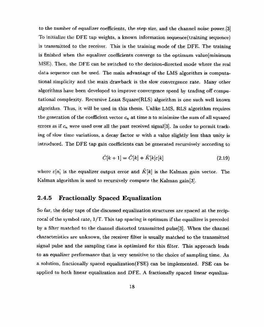
to the number of equalizer coefficients, the step size, and the channel noise powver. (31

To initialize the DFE tap weights, a knowvn information sequence(training sequence)

is transmitted to the receiver. This is the training mode of the DFE. The training

is finished when the equalizer coefficients converge to the optimum value(minimum

MSE). Then, the DFE can be switched to the decision-directed mode where the real

data sequence can be used. The main advantage of the LMS algorithm is computa-

tional simplicity and the main drawback is the slow convergence rate. Many other

algorithms have been developed to improve convergence speed by trading off compu-

tational cornplexity. Rccursive Least Square(RLS) algorithm is one such well known

algorithm. Thus, it will be used in this thesis. Unlike LMS, RLS algorithm requires

the generation of the coefficient vector c, a t time n to minimize the sum of al1 squared

errors as if c, were used over al1 the past received signal[3]. In order to permit track-

ing of slow time variations, a decay factor w with a value slightly less than unity is

introduced. The DFE tap gain coefficients can be generated recursively according to

where ~ [ n ] is the equalizer output error and ~ [ k ] is the Kalrnan gain vector. The

Kalman algorithm is used to recursively compute the Kalman gain[3].

2.4.5 Fract ionally Spaced Equalizat ion

So far, the delay taps of the discussed equalization structures are spaced a t the recip-

rocal of the symbol rate, 1/T. This tap spacing is optimum if the equalizer is preceded

by a filter matched to the channel distorted transmitted pulse[3]. When the channel

characteristics are unknown, the receiver filter is usually matched t o the transmitted

signal pulse and the sampling time is optimized for this filter. This approach leads

to an equalizer performance that is very sensitive to the choice of sarnpling tirne. As

a solution, fractionally spaced equalization(FSE) can be implemented. FSE can be

applied to both linear equalization and DFE. A fractionally spaced linear equaliza-

tion structure is shown in Figure 2.8[3]: where the delay line taps are spaced a t an

Zigure 2.8: Fractionally spaced linear equalizer

interval T which is less than the symbol interval T. T is typically selected such that

the bandwidth occupied by the signal at the equalizer input satisfies the sampling

theorem. In digital implementation, T is selected to be AT/B where A and B are

integers and B > .1. The equalization output is given by

The adaptive algorithms discussed in section 2.4.4 can also be used for FSE. -4s an

esample, the LMS algorithm(2.18) can now be written as:

Because of the higher sampling rate, FSE can effectively compensate for more severe

delay distortion and deal with amplitude distortion with less noise enhancement than

a T spaced equalizer.

2.5 Equalizat ion for Noncoherent Systems

The implementation and operation of coherent detection is a complex process in-

volving many ancillary functions associated with the carrier synchronization loop, for

esample, acquisition, tracking, lock detection, etc. In many applications, it is more

desirable to have simple aud robust implementation than have the best possible sys-

tem performance. Therefore, noncoherent detection schemes are more attractive. In

t his t hesis, we will use differential detection. Since the nonlinear nature of differential

detection and the presence of frequency selective fading channels make linear equal-

izat ion a less t han sat isfactory choice, Noncoherent DFE(NDFE) will be considered.

LVe will now discuss some of the known NDFE schemes.

-4 noncoherent equalizer for DQPSK under frequency-selective mobile radio chan-

nels with differential detection is proposed by Kohama et a1.[24]. A block diagram

of the receiver is shown in Figure 2.9. This equalizer adjusts the decision thresholds

received sign T

-f T*

Data Output -

Figure 2.9: Block diagram of the RANI based equalizer

adaptively by decision feedback. The threshold control signal is stored in a Ran-

dom Access Memory(RAM) during the training period. As the training signal starts,

the signals are sampled and stored. The sampled signals are mapped in a complex

plane. Decision boundaries are drawn to separate four signal points and stored in the

threshold data Ra4M. Because the transmit ted training data is known, it is possible

to determine which region corresponds to a data signal among the four signal points.

The result is then written in a classifying R-AM. The information data can then be

determined by finding out which region the sampled information signal falls in the

classifying RA4hI.

The performance of an indoor radio system with DQPSK modulation in frequency

selective fading channels has been studied by Benvenuto et a1.[25]. Based on the

nonlinear echo canceler given in [26], a nonlinear equalizer is proposed with differential

detection. A block diagram of the receiver is shown in Figure 2.10. The structure

Figure 2.10: Block diagram of another RAM based equalizer

received signal +n - - - Data Output t

of the filter taps of the proposed equalizer is based on the table look-up method

which takes the form of RAMs. The update of the coefficients is achieved by adding a

scaled portion of error signal to the current R-431 contents. The equalizer employ two

RAMs; one for removing the noniinear ISI due to the multiplication in the differential

detector and the other one for compensating the additive interference. The content

of each RAM location is determined by making use of a training sequence. The

equations for updating the R.4M locations are based on the LMS algorithm. Since

[24] and [23] both employ RAMs, they are not robust compared to conventional DFE

when various channels are considered.

-4 more robust NDFE structure is proposed by Masoomzadeh-Fard et al. for

4 IL -

Differential Phase Shift Keying(DPSK) under multipath fading channels[27]. The

Noncoherent receiver is illustrated in Figure 2.1 1[27]. In the Figure, rk is the received

! computation of nonlinear terms of ISI(Xk )

adaptation 1

Figure 2.11 : A noncoherent decision feedback equalizer

signal(after T sampling), which has been differentially encoded at the transmitter.

After receiving rk, a conventional differential detector is applied to remove the ab-

solute phase of the received signal. In the next stage of the receiver, the nonlinear

ISI caused by differential detection is caltulated by using decision feedback. They

are then weighted and summed in a conventional equalizer. Finally, the equalizer

output is quantized to form the decision âk, which should be equal to the original

transmitted symbol a k if no error occurs. In addition, it is shown that for nonlinear

phase channels, the differential detector creates large amounts of phase distortion and

therefore, a T-spaced nonlinear equalizer is unable to equalize these channels. The

authors proposed a fractionally-spaced NDFE structure which significantly outper-

forms the T-spaced NDFE structure. Hoivever, in the proposed NDFE algorithm, a

nonlinear processor with 0 (L2) complexity is used to determine the elements in the

equalizer input vector, where L is the number of significant symbol-spaced multipath

components in the channel[28]. Jones et al. [28] used the same NDFE structure, but

provided a more computationally efficient DFE algorithm. However, the proposed

NDFE structure is suboptimum and cause a large loss in power efficiency(typical1y

more t han 4 dB) when compared \vit h coherent DFE[29]. Schober et al. [29] proposed

a high performance NDFE scheme for the ISI channel. This scheme is derived from

optimum noncoherent MLSE and can approach coherent Minimum Mean Square Er-

ror (AIMSE) DFE arbitrarily close[29]. So Far, no other combination of an equalizer

and a noncoherent detector has been reported in literature, which can approach the

performance of a corresponding coherent receiver[30]. For adaptation of the feed-

forward and feedback filters, efficient novel modified Least Mean Square(LMS) and

Recursive Least Square(RLS) algorit hms are provided. Simulations confirm that the

proposed adaptive NDFE schemes are robust against frequency offset. The details of

this NDFE scheme will be further described in the following chapter.

Chapter 3

Demodulating GMSK wit h

Adaptive DFE in AWGN Channel

The previous chapter gives an overvieïv on GMSK, the Laurent representation of

CPM, signal detection schenies, fading channel and some typical coherent and nonco-

herent equalization techniques. We learned that due to its low implementation costs

and robustness against frequency and carrier phase offsets, differential detection, a

noncoherent signal detection schemes, is can be more advantages over coherent signal

detection schemes in a fading channel. In addition, we learned that under severe

fading channel, such as channels with spectral null, DFE is a better suboptimum

equalization technique than LE.

This chapter discusses the design issues of a noncoherent GMSK receiver based

on the Laurent representation under .\\VGN channel. Section 3.1 derives a reduced

complesitÿ PSI<-based GMSK demodulator. Section 3.2 discusses the use of coherent

DFE with the GMSK demodulator. The BER performance of the overall coherent

receiver structure will be used as the performance benchmark. Section 3.3 discusses

the use of noncoherent DFE with the GMSK demodulator. Section 3.4 discusses the

use of fractionally spaced DFE with the GMSK demodulator. For convenience of

simulation, we will use GMSK with Global System Mobiles(GSM) standard, ïvhich

specifies a BT of 0.3. Thus, ive truncates the GMSK frequency pulse to 3T.

3.1 The Laurent Approximation of GMSK Signals

It las shoivn by Laurent [31] that any binary CPM signal ivith modulation filter

duration L can be rvritten as a sum of 2L-1 P-AM signals. By applying this result, we

can write the transmitted G-VISK signals with BT=0.3 and L=3 as the sum of four

P-AM modulated signals:

where k is the P-Mil pulse index, n is the indes of the current bit of the input sequence,

and

~ [ n ] = ao[n - l ] j Q ~ * ] with,

j = e'f and a[n] E 1,-1

The other ak[n] have the following general form:

ak[n] = ao[n - 3) n ja["-'1 , k = 1 ,2 ,3 i f I k

witli, Ik c {O, 1, 2)

The P-4M pulses are expressed as:

where, B(t ) is defined as:

s n ( ( 1 - q t ) ) : O 5 t 5 3T

B(-t) : - 3 T L t s O

q ( t ) is the GMSK phase shaping filter discussed in Chapter 2. Numerical integration

of the main Laurent pulse, ho, shows that it contains 99.7% of t he total GMSK pulse

energy. Thus, s ( t ) can be well represented in terms of ho(t) only. The pulse shape

for ho is shown in Figure 3.1. Note that although ho is defined over 4T, the main

Time (units of T)

Figure 3.1: The Laurent main pulse

pulse energy is contained within 3T. ho can then be truncated t o 3T. By using only

ho, s ( t ) can be further simplified to:

From (3.2), if ive assume that the initial s tate of ao[n] = 1 and note that jQLnl = ja[n],

ive can rewrite s( t) as:

where, a& - 11 E {f 1, f j } , or

tvhere, a[n] E {&l}. A block diagram of an one-pulse(1P) approximation of GMSK

modulator is given in Figure 3.2.

Figure 3.2: The Laurent modulator

3.1.1 Approximating GMSK as Binary Differential PSK

The approsimated GMSK modulator consists of a differential encoder, an I/Q m a p

per(mhich can also be seen as a 90 degree phase rotation), and a transmitter filter,

ho. In this sect,ion, me will show tha t with a simple derotation a t the receiver, tve can

approsimate the Laurent-based G MSK transmission system by a Binary Different ial

PSK(BDPSK) transmission system. Figure 3.3 shows a block diagram of the discrete-

time 1 P approsimated GMSK transmission model. The received signal, sampled a t

times kT a t the output of the receiver input filter can be written as: Lh-1

r [k] = h, a [k - n ] jk-" + n [k] n=O

where a [ k ] is the antipodal input symbol and a[k] = a [ k ] a [ k - 11. h,, O 5 n 5 Lh - 1,

are the coefficients of the combined discrete-time impulse response of the transmit

filter, channel, and receiver input fi1ter;its length is denoted by Lh. n [ k ] represents

comples additive Gaussian noise with a one-sided power spectral density of No. First

we recognize that:

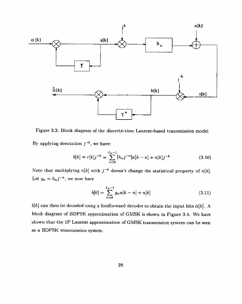
Figure 3.3: Block diagram of the discrete-time Laurent-based transmission mode1

By applying derotation j-', we have:

Lh-L

b[k] = r [k] j-' = [h,j-"]a[k - n] +n[k]j-k (3.10) n=O

Note that multiplying n[k] with j-' doesn't change the statistical property of n[k].

Let g, = h, j d n , we now have

b[k] can then be decoded using a feedforward decoder to obtain the input bits &[k]. -4

block diagram of BDPSK approsimation of GMSK is shown in Figure 3.4. We have

shown that the 1P Laurent approximation of GMSK transmission system can be seen

as a BDPSK transmission system.

Figure 3.4: Block diagram of the discrete-time BPSK-based transmission model

3.2 Detecting GMSK with A Coherent Adaptive

DFE

If synchronization is possible and inexpensive, it is well known that a coherent de-

tection scheme outperforms a noncoherent detection scheme. Therefore, we will first

implement a coherent PSK-Based GMSK receiver. The performance of the coherent

scheme will be used as a benchmark for the noncoherent scheme. For simplicity, we

will derive the receiver using the BDPSK transmission model shown in Figure 3.4.

In a coherent -4WGN channel, matched filtering is an optimal front-end for the re-

ceiver because it maximizes the SNR and provides sufficient statistics for detection.

Therefore, the receiver filter is matched to the main Laurent pulse. However, this

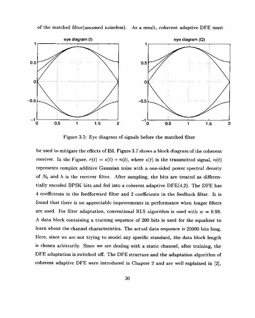
matched filtering introduces additional ISI. This is clearly shown in Figure 3.5 and

Figure 3.6. Figure 3.5 shows the eye diagrams for the signal(1 and Q ) a t the input of

the matched filter and Figure 3.6 shows the eye diagrams for the signal at the output

of the matched filter(assumed noiseless). As a result, coherent adaptive DFE must

eye diagram (1) eye diagram (O)

Figure 3.5: Eye diagram of signals before the matched filter

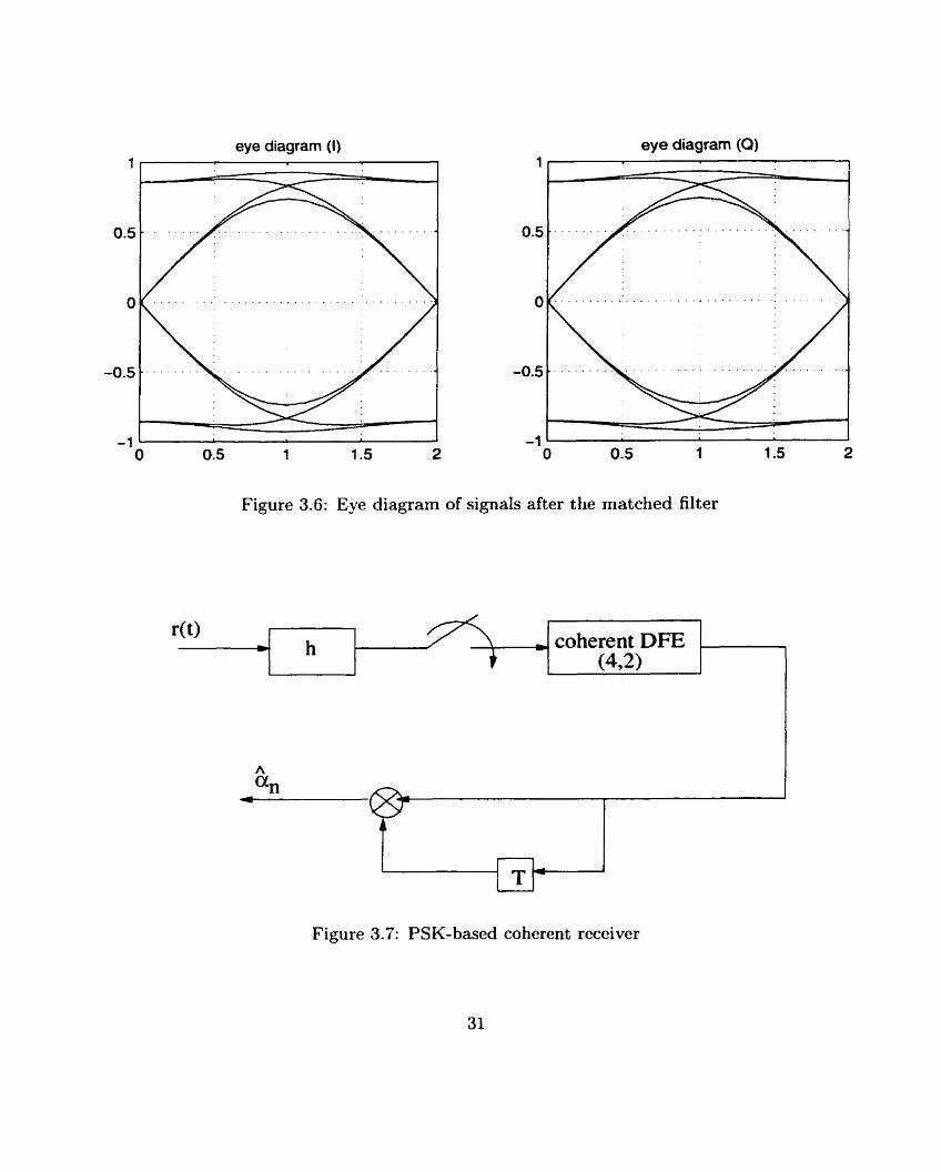
be iised to rnitigate the effects of ISI. Figure 3.7 shows a block diagram of the coherent

receiver. In the Figure, r ( t ) = s(t) + n(t) , where s ( t ) is the transmitted signal, n(t)

represents complex additive Gaussian noise wit h a one-sided power spectral density

of No and h is the receiver filter. .4fter sampling, the bits are treated as differen-

tially encoded BPSK bits and fed into a coherent adaptive DFE(4,P). The DFE has

4 coefficients in the feedforward filter and 2 coefficients in the feedback filter. It is

found that there is no appreciable improvements in performance wlien longer filters

are used. For filter adaptation, conventional RLS algorithm is used with w = 0.98.

A data block containing a training sequence of 200 bits is used for the equalizer to

learn about the channel characteristics. The actual data sequence is 20000 bits long.

Here, since we are not trying to mode1 any specific standard, the data block length

is chosen arbitrarily. Since we are dealing with a static channel, after training, the

DFE adaptation is switched off. The DFE structure and the adaptation algorithm of

coherent adaptive DFE were introduced in Chapter 2 and are well explained in [2],

eye diagram (1)

Figure 3.6: Eye diagram of signals after the matched filter

Figure 3.7: PSK-based coherent receiver

we will not discuss it further here. In this thesis, the signal to noise ratio(SNR) is

defined as Eb/No

3.2.1 Coherent GMSK Receiver Performance

In ordcr to find the performance loss due to the 1P approximation, the PSK-based

cotierent receiver shown in Figure 3.7 will be used to receive actual GiMSK sig-

nals(generated by Figure 2.1) and approximated GMSK signals (generated by Figure

3.2). Since the receiver is designed according to the 1P approximation of GMSK, we

espect the performance of the receiver receiving actual GMSK signals to be worse

tlian the performance of the receiver receiving the approsimated GLMSK signals. Fur-

thcrmore, since the 1 P approximation contains most of the GMSK energy, ive expect

the performance difference to be small. However, computer simulation results contra-

dict our espectation. Froni Figure 3.8, ive see that the receiver receiving the actual

G h4SK signals performs much worse t han receiving the approximated G MSK signals.

Further analysis shows that when receiving real GPvlSK signals, the DFE filter taps

hiled to converge. This indicates that the ISI may be time-varying.

3.2.2 Sirnulating GMSK

In section 2.1.1, ive mentioned that g(t), the GMSK frequency pulse is normally

truncated to LT. For GkISK with BT=0.3, L is chosen to be 3. When simulating the

GMSK modulator, Ive used the truncated g(t). Since the phase function q(t) is the

integral of g(t), the truncation of g(t) causes instability of GMSK phase. This insta-

bility in turn causes the instability of DFE algorithm. To illustxate this, assume that

the GMSK modulator presented in Figure 2.1 is used to modulate an al1 1 input data

block. IdealIy, the phase of the modulated signals should be a linear continuously

increasing function. Figure 3.9 shows the plot of such a function(phase is normally

represented between T and -w). When truncation is applied to g(t), it creates dis-

continuity in the phase function. Figure 3.10 shows that the truncation loss causes

. . . . . . . . + . . . . . . . . . . . . . . . . . . . . . ; : : : : : : ': : : : : : : :':. . . . . . . L - W . .

. . . . . . . a . . . . . . . . . . . . . . . . . - . . . . . . . . . . . . . . . . . . . . . . . . . . . 1 + GMSK signais

. . . . . . . . . . . .

. . . . . . . . . . . . . . . . . . . . . . . . . . . . . . . . . . . . . . . . . . . . . . . . . . . . . . . . . . .

SNR (dB)

Figure 3.8: BER performance of the PSK-based receiver receiving 1P approximated

GMSK signals and GMSK signals in an .4WGN channel

the phase of GiLISK signal t o fluctuate. This fluctuation in turn caused the ISI to

be time-varying. Therefore, the initial training of DFE did not provide convergence.

To solve this problem, a truncation of L = ï is used in the simulation of GMSK modu-

lator. Note that to obtain a Laurent representation, L=3 is still sufficient. Using the

improved GMSK modulator, Figure 3.11 shows that the performance of the receiver

receiving the actual GMSK signals is very close to the approximated GMSK signals.

Therefore, GbISK can be well approximated as BDPSK in a coherent system.

3.2.3 Sensitivity to Frequency Offset

One of the major problem of coherent detection scheme is its sensitivity to frequency

offsets. However, a practical wireless charinel sornetimes introduces phase drift, which

would cause frequency offset. This can be represented by r ( t ) e j tAf , where r ( t ) is the

received signal. Coherent adaptive DFE can not cope with this impairment even when

O 500 1 O00 1500 2000 2500 sample number

Figure 3.9: Ideal phase plot of GMSK signals with al1 Is as input

O 500 1 O00 1500 2000 2500 sample nurnber

Figure 3.10: Phase plot of GMSK signals with al1 1s as input and L=3

. . . . . . . . . . . . . . . . . . . . - . . . . loO 1 : : : : : : : :::: : : : : :.:. . . . . . ' , ' . . . . . . . . , . . . . . . . . . .

: : : : : : : : : : : : : : : : ::: ' -8 GMSK signais : : : : : : : : : : : : : : : : ::: -iic 1 P approximated GMSK signals :: . . . . . . . . . . . . . . . . . . . . . . . . . . . . . . . . . . . . . . . . . . . . . . . . . . . . . . . . . . .

1 1 I I I 1 l 2 3 4 5 6 7 8 9

SNR (dB)

Figure 3.11: Performance of the PSK-based receiver receiving 1P approximated

GMSK signals and GMSK signals

running in decision directed mode. In Figure 3.12, the performance of the coherent

receiver receiving GlMSK signals is evaluated for a constant frequency offset A f a t

S N R = 8dB. We see that coherent adaptive DFE fails to equalize even for very small

frequency offsets. This shows that the conventional RLS algorithm is unable to track

the phase variations[2].

3.3 Differential Detection of GMSK signals with

Adaptive NDFE

We have seen that coherent equalizers are not capable of compensating for the time-

varying phase. In addition, in many applications, it is not possible to perform coherent

detection due to the inability of the receiver to produce carrier phase estimates.

Therefore, differential detection, which obviates the need for implementing the carrier

Figure 3.12: Probability of error versus 4 f T for coherent detection

synchronizat ion function, is an attractive alternative to coherent detection. In chapter

2, we briefiy introduced Schober's NDFE scheme. In this section, we wili discuss

detecting GMSK signals with Schober's adaptive NDFE.

3.3.1 Schober's Adaptive NDFE

Schober7s adaptive NDFE scheme is proposed for M-ary differential PSK signals.

First, we will discuss in more detail the NDFE algorithm. Figure 3.13 shows a block

diagram of a complex baseband discrete-time M-ary differential PSK transmission

mode1 used in deriving the algorithm[29]. The information symbols a[k] E {ej2""/" 1 v E {O, 1, ..., M - l}}, which are independent and identically distributed random

variables, are differentially encoded into the symbols b[k] as follows:

where b[O] = 1. The transmitter filter has a real impulse response corresponding to

square-root raised cosine spectrum. The receiver filter is matched to the transmitter

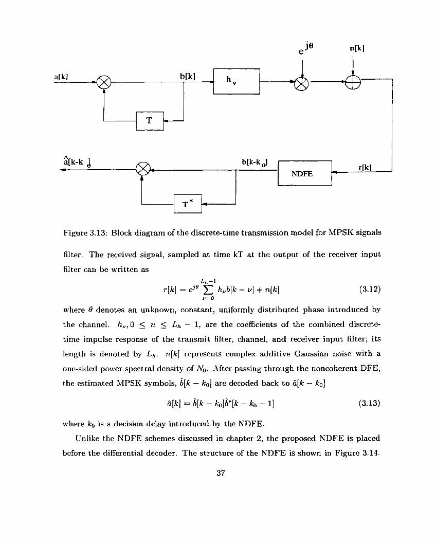
Figure 3.13: Block diagram of the discrete-time transmission mode1 for MPSK signals

filter. The received signal, sampled a t time kT at the output of the receiver input

filter can be written as

where 0 denotes an unknowri, constant, uniformly distributed phase introduced by

the channel. h,, O 5 n 5 Lh - 1, are the coefficients of the combined discrete-

time impulse response of the transmit filter, channel, and receiver input filter; its

length is dennted by Lh. n[k] represents complex additive Gaussian noise with a

one-sided power spectral density of No. After passing through the noncoherent DFE,

the estimated MPSK syrnbols, b[k - ko] are decoded back t o â[k - ko]

where ko is a decision delay introduced by the NDFE.

Unlike the NDFE schemes discussed in chapter 2, the proposed NDFE is placed

hefore the differential decoder. The structure of the NDFE is shown in Figure 3.14.

In the Figure, r D F E [ k ] is the output of the NDFE feedforward(FF) filter, YDFE[k] is

Figure 3.14: Block diagram of Schober's NDFE structure[29]

the output of the NDFE feedback(FB) filter. The FF filter coefficient vector f F [ k ]

with length L F , the FB filter coefficient vector f B [k] with Length LB and the received

signal sarnples vector R[k] with length LF are defined as:

R[k] A [ r [ k ] r [ k - 11 ... r [ k - LF i- 1]IT

' [ ~ B . o [ ~ ] f ~ , i [ k ] .-- fL?,(L,- i> [ k ] l x

Siiice FF and FB filters introduce an additional degree of design freedom, the con-

strain f B y o [ k ] E 1 is used. Thus

From -4ppendi.u A, me see that the NDFE might be interpreted as a noncoherent

reduced state MLSE with only one state. The resulting DFE decision rule is given as

where

b[k - ko] is the decision,

and

Note that the decision rule does not depend on the channel phase 0 which is manda-

tory for a noncoherent receiver. -4s a result, differential encoding is needed since the

absolute phase of the estirnated symbol sequence b[k] rnay differ from the absolute

phase of the transmitted symbol sequence b[k] . The phase of Q,[k - 11 is inter-

preted as an estimation of the phase difference between rDFE[k] and $oFE[k]. Thus,

as N increases, the accuracy of the estimation improves. However, increasing N also

increases the required number of computations. Tiierefore, instead of the summation

form, a recursive met hod can be used to estimate the phase difference:

AN-1 where ,û, O 5 < 1, is a forgetting factor. Note that q,,, [k - 11 and qrec[k - 11 are

identical as N + oo and ,B + 1.

Since this is a noncoherent scheme, there is no simple filter design criterion based

on minimization of an error variance. Therefore, E { D [ k ] ) is used as the cost function

for calculation of the FF and FB filters. The filter settings for f F [ k ] and fB[k] can

be calculated from

where O s , denotes the al1 zeros vector with Sx rows. For finite N, it is very difficult

to find the solution analytically. The authors derived the modified LMS and RLS

algorit hms to find the desired filter settings[29]. For illustration purpose, the modified

LMS algorithm is given below:

The FF filter coefficient vector is updated according to

wit h

where 6 is the adaptation step size. Similarly, the feedback filter coefficients can be

updated as

f ~ [ k + 11 = fB[k] + bekc[k]

with

To calculate eF[k] and es[k], knowledge of the transmitted symbol sequence b[k ] is

necessary. Therefore, a training sequence is needed for adaptation of the FF and FB

filter coefficients. The modified LMS algorithm is very similar to the conventional

LW. When compared to conventional LMS algorithm, the only difference is the factor

and for calculation of eF[k] and ee [k]. Furthermore, at time k = O, al1 I+ec[kIl

FF and FB filter coefficients are initialized with zeros. At k = 1, Iqrec[kII - - 1 is used.

ko7 the delay introduced by DFE,can be determined by using ko = LF + Lh - 1 - LB.

It is shown both analytically and through simulation that as P increases, the

performance of the proposed NDFE increases[29]. As f l -+ 1, the performance of

the NDFE is the same as coherent DFE. To illustrate this, we will compare the

performance of a coherent DFE(4,2) with the NDFE(4,2) by iising the proposed PSK-

based receiver receiving 1P approximated GMSK signals. Figure 3.15 shows that at

,!3 = 0.9, there is onlÿ a very small difference. It is shown in last section that the

. . . . . . . . . . . . . . . . . . . . . . . . . . - . . . . . . . . . . . . . . . . . . . . . . . . . . . . . . . . . . . . . . . . . . . 1 - 0 - Coherent DFE 11

- -

2 3 4 5 6 7 8 9 SNR (dB)

Figure 3.15: BER Performance of the PSK-based receiver receiving 1 P approximated

GMSK signals with coherent DFE versus NDFE at P = 0.9

coherent DFE fails to function when a frequency offset is present, and the NDFE can

track this frequency offset by decreasing P . It is shown through simulation that as @

decreases, the frequency sensitivity decreases as well[29]. This will be demonstrated

later in the chapter. Therefore, for the NDFE, there is a tradeoff between performance

and sensitivity to frequency offset.

3.3.2 Noncoherent GMSK Receiver Performance

From section 3.1.1, ive see that GMSK can be well approximated as BDPSK in co-

herent system. Therefore, we will apply Schober's DFE algorithm directly to GMSK

signals. For the simulations, the modified RLS algorithm(presented in Appendix B

along with its learning curve) with w = 0.98, is used for adaptation of NDFE taps.

For each data block, the training sequence is 200 bits long and the actual data is

20000 bits long. To have a fair cornparison, the NDFE has the same number of FF

and FB filter taps as the coherent DFE. Since the outputs of matched filter are suf-

ficient statistics for syrnbol detection, ive will continue to use the rnatched filter as

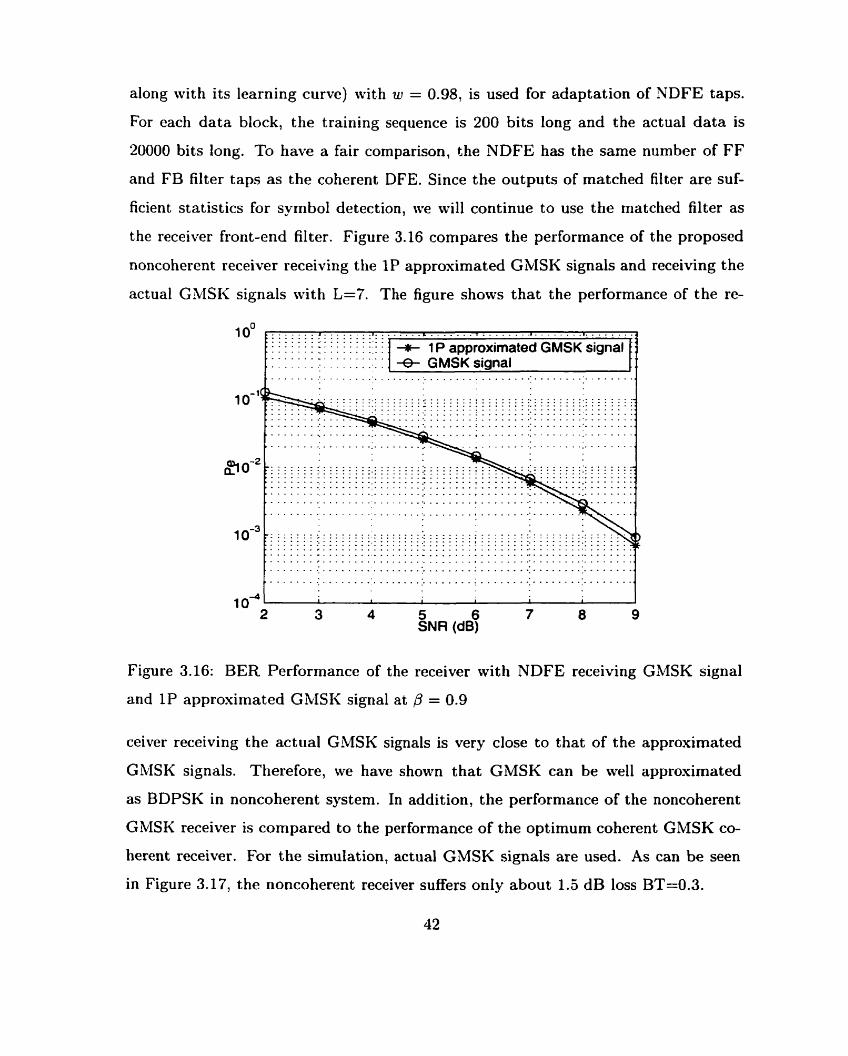
the receiver front-end filter. Figure 3.16 compares the performance of the proposed

noncoherent receiver receiving the 1P approximated GklSK signals and receiving the

actual GMSK signals with L=7. The figure shows that the performance of the re-

10" : : : ,: : : : : : : :.::. . . . . . . . . . . . . . . . . . .,. . . . . . . . . . . . . . . . . . . . . . . a ,. . . . . . . . . . .

: : : : : : : : : : : : : : : : :.: : ' + 1 P approximated GMSK signal !! . . . . . . . . - . . . . . . . . . . . . . . . . . . . . . . . . . . . . . . . : + GMSK signal . . . . . . . . . . . . . . . . . . . . . . . . . . . . . . . . . . . . . . . . . . . . . . . . . . . . . . . . . . .

2 3 4

Figure 3.16: BER Performance of the

and 1P approsimated GMSK signal at

5 6 SNR (dB)

receiver with NDFE receiving GMSK signal

0 = 0.9

ceiver receiving the actiial G-MSK signals is very close to that of the approximated

GMSK signals. Therefore, we have shown that GMSK can be well approximated

as BDPSK in noncoherent system. In addition, the performance of the noncoherent

GMSK receiver is compared to the performance of the optimum coherent GMSK co-

herent receiver. For the simulation, actual GMSK signals are used. As can be seen

in Figure 3.17, the noncoherent receiver suffers only about 1.5 dB loss BT=0.3.

. . . . . , . - . . . . . . .

2 3 4 5 6 7 8 9 SNR (dB)

Figure 3.17: BER Performance of optimum coherent receiver versus proposed nonco-

herent receiver a t ,l3 = 0.9

3.3.3 Sensitivity to Frequency Offset

In this section, we will investigate the sensitivity of the proposed noncoherent GMSK

receiver to frequency offset. Frorn here on, actual GMSK signals are used for al1

simulations and the performance of the coherent GMSK receiver is included when

appropriate. Figure 3.18 compares the performance of the receivers with P = 0.9,

,b' = 0.6 and B = 0.4. The plot verifies that as P increases t o 1, the performance of

the noncoherent receiver approaches the performance of the coherent receiver. The

noncoherent receivers are then compared for their ability to handle frequency offset.

For the simulation, a constant frequency offset 4 f a t SNR = 8dB is introduced.

Figure 3.19 show that though P = 0.4 performs the worst when no frequency offset

is present, it is the best when severe frequency offset is present. Hence we have

shown that there is a tradeoff between the receiver's sensitivity to frequency offset

and its performance. To explain this tradeoff, we have to take a close look at the

NDFE structure. The phase of q,.& - 11 might be interpreted as the estimate for

the phase difference between rDFE[k] and yDFE[k ] . If we assume the phase differencc

is a constant value(no frequency offset), as 0 + 1, the accuracy of this estimate

increases, which improves the performance. However, if the phase difference is time

variant value(frequency offset is present), as 0 + 1, the phase of q& - 11 cari not

be used to track the changes in the phase difference. Smaller value is more robust

for the changes, which results in better performance.

5 6 SNR (dB)

Figure 3-18: BER Performance

3.3.4 The Role of BT

So far, we only considered GMSK

of the noncoherent receiver with different ,B

with BT = 0.3. This section investigates the

performance of the noncoherent receiver for different BT vaIues. From chapter 2, ive

have seen that by increasing BT, the duration of GMSK phase function is reduced.

This reduction in duration translates to reduction in duration of Laurent pulses L,

thus, less ISI. Therefore, it is expected that as BT increases, the BER performance of

Figure 3.19: Probability of error versus A f T for the noncoherent receiver with dif-

ferent fl

the noiicoherent receiver will increase. This is verified in Figure 3.20. In the figure,

the performance of noncoherent detection of DBPSK and MSK are also plotted for

reference. The probability of error for DBPSK and EVISK in AWGN channel are given

However, as BT increases, the spectral

shows the power spectrum of the GMSI(

efficiency of GMSK decreases. Figure 3.21

signal versus the normahzed frequency wi t h

BT as a parameter. This figure is generated by using Urelch's method for spectrum

estimation. [37] Therefore, there is a. tradeoff between performance and spectrum effi-

ciency for the proposed receiver.

Figure 3.20: BER Performance of the noncoherent receiver with different BT and L

Welch PSD Estimate

Figure 3.21: Power spectra of GMSK

3.3.5 Fractionally Spaced NDFE

For liriear modulation, the optimum receiver filter is the cascade of a filter matched

to the actual channel, with a transversal T-spaced equalizer[2]. By reducing the sam-

pling phase sensit ivity relative to T-spaced equalizer, the fractionally spaced equalizer

can synthesize the best combination of the matched filter and a T-spaced equalizer for

maximum likelihood detection. This advantage is not as important for GMSK modu-

lation since there is no single receiver filter that can match exactly to the transmitter

filter. In addition, the difference between the best and worst timing epochs is much

smaller for the DFE than for a LE[21]. Therefore, for GMSK modulation, fractionally

spaced NDFE has no performance advantage over T-spaced NDFE. This is verified

by computer simulation by using the proposed NDFE, for BT = 0.3, f l = 0.9. The

feedforward t ap spacing of the fractionally spaced NDFE is 5 . To cover the same

channel span as T-spaced NDFE, fractionally spaced NDFE requires twice as many

FF filter taps as the T-spaced NDFE. The simulation result is shown in Figure 3.22.

The figure shows no performance improvement by using fractionally spaced NDFE.

Similar result is also reported in [22] for coherent detection of GMSK signals.

3.3.6 Performance Versus Ot her Noncoherent GMSK Re-

ceivers

It was shown that a t p = 0.9, the proposed noncoherent GMSK receiver performs

very close to a corresponding coherent receiver. In addition, we will compare the pro-

posed receiver a t p = 0.9 to three other noncoherent receivers presented in [38],[15]

and [39]. In [38], Korn proposed a noncoherent GMSK receiver by employing limiter-

discriminator and Zbit decision feedback. In [15], Yongacoglu e t al. proposed a

noncoherent GMSK receiver by combining 2 and 3-bit differential detection and deci-

sion feedback. In [39], Colavolpe e t al. proposed a noncoherent GMSK receiver based

on noncoherent sequence detection using the Viterbi algorithm with 32 states. It is

1 041 . , , fi I , j 3 4 5 6 7 8 9

SNR (dB)

Figure 3.22: BER Performance of the receiver with T-spaced NDFE and T/2-spaced

NDFE

found that the receiver proposed by us is slightly more computationally complex than

the receivers proposed by Korn and Yongacoglu. Hotvever, the receiver proposed by

Colavolpe is much more complex than the receiver proposed by us. Table 3.1 com-

pares the BER performances with BT = 0.25 under AWGN channel. From the table,

ive see t hat \vit h slight ly higher computationa1 complexity, the receiver proposed by

us outperforms the receivers proposed by Korn and Yongacoglu. However, the re-

ceiver proposed by Colavolpe performs better than the receiver proposed by us a t

the price of a much higher cornputational complexity. Thus, we conclude that the

receiver proposed by us is a high performance noncoherent receiver when compared

to other known noncoherent GMSK receivers.

Table 3.1: BER performance comparison of various noncoherent receiver at BT =

0.25 under AWGN channel

SNR (dB)

BER Proposed Korn[38] Yongacoglu [l5] Colavolpe[39]

Chapter 4

Reduced-complexity Noncoherent

Receiver in Fading Channels

In the previous chapter, we proposed a noncoherent GMSK receiver. We investigated

the performance of the receiver in .4WGN channel where the primary source of error is

the thermal noise. Hoivever, in wireless systems, more errors are caused by fading and

multipath effects. Therefore, analyzing the performance of a wireless communication

system requires more complex channel models.

This chapter investigates the performance of the proposed noncoherent receiver

in fading channels. Section 4.1 investigates the receiver's performance in two static

Finite Impulse Response(F1R) channels. The cffects of parameters, P(the NDFE7s

forgetting factor) and BT(GMSK's spreading factor), on the receiver7s overall perfor-

mance will be discussed. Section 4.2 investigates the effects of the same parameters

on the overall performance of the receiver under flat Rayleigh fading channel. In

addition, the effects of multipath delay spread on the performance of the receiver will

be discussed.

4- 1 Performance Under Static Channels

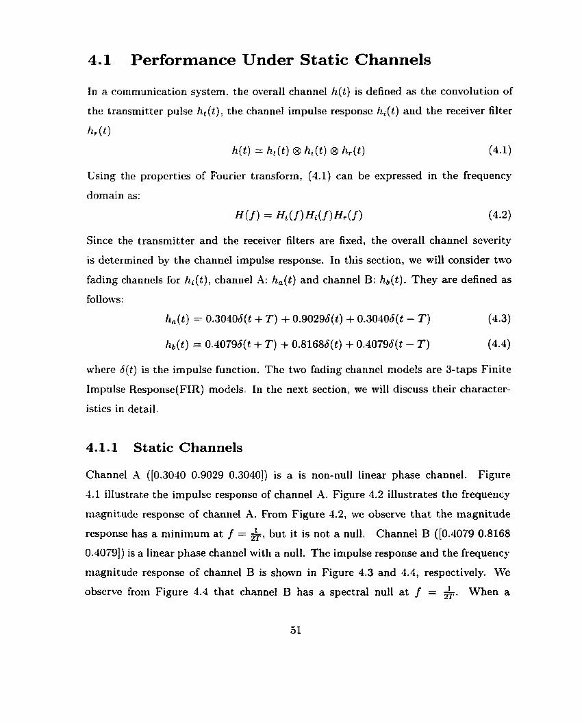
In a communication system, the overall channel h(t) is defined as the convolution of

the transmit ter pulse hl (t) , the channel impulse response hi (t) and the receiver filter

hr ( t )

h(t) = h, ( t ) 8 hi(t) 8 hr(t) (4.1)

Using the properties of Fourier transform, (4.1) can be expressed in the frequency

domain as:

Since the transmitter and the receiver filters are fixed, the overall channel severity

is determined by the channel impulse response. In this section, tve will consider two

fading channels for hi(t), channel A: h,( t ) and channel B: hb( t ) . They are defined as

follotvs:

h,(t) = 0.304Od(t + T) + 0.90296(t) + 0.30406(t - T) (4-3)

where 6 ( t ) is the impulse function. The two fading channel models are 3-taps Finite

Impulse Response(F1R) models. In the next section, ive will discuss their character-

istics in detail.

4.1.1 Static Channels

Channel A ([0.3040 0.9029 0.30401) is a is non-nul1 linear phase channel. Figure

4.1 illustrate the impulse response of channel A. Figure 4.2 illustrates the frequency

magnitude response of channel A. From Figure 4.2, we observe that the magnitude

response has a minimum a t f = &, but it is not a null. Channel B (10.4079 0.8168

0.40791) is a linear phase channel with a null. The impulse response and the frequency

magnitude response of channel B is shown in Figure 4.3 and 4.4, respectively. We

observe from Figure 4.4 that channel B has a spectral nul1 at f = p. When a

Figure 4.1: Impulse response of channel A

Impulse response

Figure 4.2: Frequency magnitude response of channel A

1

0.8

0.6 CI +- -- .c

0.4

0.2

-2T -T O T 2T t

. O

Q

9

-

-

-

O

-

1

linear transversal equalizer is used to eliminate ISI, the resulting filter is the inverse

of the channel. For channel B, i-e. channel with spectral null, the resulting filter

will have large gain a t the nul1 region. This amplifies noise in that region and czuses

more probability of error. Therefore, channel with nulls are more severe than those

channels without null. In such channels, DFE is needed.

Impulse response

Figure 4.3: Impulse response of channel B

4.1.2 Simulation Results

For the simulations? the modified RLS algorithm(w = 0.998) is used for the adaptation

of the NDFE taps. The training sequence is 500 bits long and the actual data is

20000 bits long. The NDFE has 6 taps in the FF filter and 4 taps in the FE3 filter.

Figure 4.5, 4.6, 4.7 and 4.8 show the effects of 0 (at constant BT = 0.3) and BT

(at constant B = 0.9) on the proposed noncoherent receiver under channel A and B.

The performance of the coherent receiver under each channel is also presented as a

reference. From the figures, we verify that channel B is mcre harsh than channel A.

Figure 4.4: Frequency magnitude response of channel B

Yet, the effects of @ and BT on the receivers under both channels are very similar to

the results under the AWGN channel.

4.2 Performance Under Rayleigh Fading Channels

4.2.1 Rayleigh Fading Channel Mode1

In Chapter 2, we introduced the multipath fading channel and some of its charac-

teristics. Here, Ive will look at a popular fading channel model, the Rayleigh fading

channel. If the sum of the multipath components is a complex Gaussian process, the

magnitude of the process has a Rayleigh distribution. Therefore, in a Rayleigh fad-

ing channel, the transmit ted signal is randomly modulated wit h a complex Gaussian

process denoted as z(t). The wireless channel in which only one such path exists is

known as a flat RayLeigh fading channel. When there are more than one such path

esisting, the channel is called multipath Rayleigh fading channel. In multipath fad-

1 1 I I 4 6 8 10 12 14

SNR (dB)

Figure 4.5: Performance of the receiver under channel -4 with various 0

Figure 4.6: Performance of the receiver under channel A with various BT

. . . . . . . . . . . . . . . . . . . . . . . . . . . . . . . . . . . . . . . . . . . . . - 1 . . . . . . . . - 1 . . . . . . . . . . . . . . . . . . . . . . . . . . . . . . . . . . . . . . . . . . . . . . . . . . . . . . . . . . . . . . . . . . . . . . . . . . . . . . . . . . . . . . . . . . . . . - . . . . - . . . - . . . . . . . . . . . . . . . . . . . . . . - . Coherent [ . . . . . . . . . . . . . . . . . . . . . . . . . . . . . . . . . . . . . . . . .

loa l I 1 1 1 I I

2 4 6 8 10 12 14 SNR (dB)

Figure 4.7: Performance of the receiver under channel B with various ,B

SNR (dB)

Figure 4.8: Performance of the receiver under channel B with various BT

ing channel, if the difference between each path delay, r, is significant relative to a

symbol duration, then there esists frequency selectivity in the channel, which would

introduce ISI. -4 parameter called rms delay spread, p,, is introduced to indicate the

significance of the ISI of the channel. In this thesis, we will use a two ray fading

channel model to investigate the effect of p, on the proposed receiver. The two ray

fading channel model is shown in Figure 4.9. The gain z I ( t ) and z2 ( t ) are independent

comples Gaussian processes. The two rays in the channel have the same mean power,

so the rnean rms delay spread is :.

Path 2

Figure 4.9: The block diagram of a frequency selective Rayleigh fading channel

.-

4.2.2 Simulation Results

. z ,O) Signais at Path 1

To simulate Rayleigh distribution, 1000 zero mean, unit variance, comples Gaussian

raridom variables are generated. For the simulations, the modified RLS algorithm(w =

0.998) is used for adaptation of NDFE taps. The training sequence is 500 bits long

and the actual data is 20000 bits long. The NDFE has 6 taps in the FF filter and

4 taps in the FB filter. Figure 4.10 and Figure 4.11 shows the effects of /3 and BT

on the proposed noncoherent receiver under flat Rayleigh fading channel. In Figure

4.10, the performance of noncoherent detection of DBPSK and MSK are also plotted

for reference. The probability of error for DBPSK and MSK in flat Rayleigh fading

the output of the

transmitter

C

Rayleigh faded signal - C - Z

channel are given as [2] : 1

The figures show that the general trend of the effects of the parameters are similar

to the case of the -4WGN channel. However, the degree is much reduced. It was

men tioned t hat frequency selective fading, caused by multipat h delay spread, causes

ISI. If equalizers are not used, the ISI can result in an irreducible BER floor. Figure

4.12 shows the effect of delay spread on the performance of the proposed receiver. It

was confirmed through simulation that as SNR + oo, there was no BER floor forming

with increasing delay spread. When compared to flat Rayleigh fading, because of

channel diversity, the performance of the receivers with channel delay spread greater

than O.5T are better than the performance of the receiver under flat Rayleigh fading

channel.

a II

. . . . . . . . . . . . . . . . . . . . . . . . . . . . . . . . . . . . . .

. . . . . . . . . . . . . . . . . . . . . . . . . . . . . . . . . . . . . . . . . . . . . . . . . . . . . . . . . .

1 o - ~ 1 1 I L

8 10 12 14 16 18 20 22 SNR (dB)

Figure 4.10: Performance of the receiver under flat Rayleigh fading channel with

various 0

I 1 1 I l 8 10 12 14 16 18 20 22

SNR (dB)

Figure 4.11: Performance of the receiver under flat Rayleigh fading channet with

various BT

Figure 4.12: Performance of the receiver under multipath Rayleigh fading channel

with various r

Chapter 5

Conclusion

5.1 Summary of Results

In this thesis, we proposed a reduced complexity noncoherent receiver for GMSK

signals. The main body of the thesis is divided in to three parts. In chapter 2, we

have given an overview on GMSK, the Laurent representation of CPM, signal detec-

tion schemes, fading channel and some typical coherent and noncoherent equalization

techniques. In chapter 3, Ive have investigated the design issues of the noncoher-

ent GMSK receiver based on the Laurent representation under AWGN channel. In

cliapter 4, we have evaluated the proposed noncoherent receiver in fading channels.

In chapter 2, it was noted that due to its low implernentation costs and robustness

against frequency and carrier phase offsets, differential detection, a noncoherent signal

detection scheme, may be more advantageous over coherent signal detection schemes

in fading channel. It was also shown that a coherent Laurent-based MLSE GMSK

demodulator requires 4 x 2L-1 states in AWGN channel. If channel-induced ISI is

also considered, more states must be added. As a result, the overall computational

complcxity of the receiver will be too high to implement. Therefore, suboptimurn

channel equalization schemes are used to combat ISI. We learned that under severe

fading channel, such as channels with spectral null, DFE is a better suboptimum

equalization technique than LE.

In chapter 3, it was discovered that by using Laurent one-pulse approximation

of GMSK and a derotation process, a GMSK system can be well approximated by

DBPSK system. Thus, a high performance PSK-based NDFE scheme can be applied

directly to GMSK signals. It was shown that the performance of the proposed nonco-

herent receiver can approach the corresponding coherent GMSK receiver. In addition,

it was shown that the proposed noncoherent receiver suffers only about 1.5 dB loss

when compared to the optimum coherent GMSK receiver. Two int rinsic paramet.ers

(BT and B ) were also esamined to see their effects on the performance. Furthermore,

the performance of the proposed noncoherent receiver is compared to other known

noncoherent GMSK receivers. The result concluded t hat the proposed receiver has

high performance.

In chapter 4, the proposed noncoherent receiver was examined for fading chan-

nels. The receivers, along with the two parameters, were first exarnined under static

fading channel with deterministic properties. They w r e then esamined under quasi-

static flat Rayleigh fading channels. Finally, the receiver was examined under two-ray

Rayleigh fading channels with different multipath delay spread. Figure 5.1 shows that

a t /3 = 0.9 and BT=0.3, the performance were poorer going from -4kVGN channel to

static fading channels then to flat Rayleigh fading channel. It is concluded that in

multipath Rayleigh fading channcl, due to path diversity, the performance of the re-

ceivers with channel delay spread greater than 0.5T are better than the performance

of the receiver under flat Rayleigh fading channel.

5.2 Suggestions for Future Work

We used two ray Rayleigh fading channel mode1 to study the effects of multipath delay

spread on the proposed receiver. In a real wireless communication channel, there are

greater number of rays. Therefore, more accurate fading channel models can be used

. . . . . . . . . . . . . . . . . . . . . . . . . . . . . . . . . . . . . . . . . . . . . . . . . . . . . +-Rat Rayleigh ~ading~hannel . . . . . . . . . . . . . . . . . . . . . . . . . . . * Channel 0

Figure 5.1: BER Performances of the proposed noncoherent receiver a t ,B = 0.9 under

various channels

to further evaluate the receiver. In addition, instead of simulated fading channels, real

fading channels may be used to evaluate the performance of the proposed receiver.

This could be done by using measured channel responses.

In a practical wireless communication systems, channel coding is usually used

to improve the performance of the overall system. Furtherrnore, adding an error-

correcting code involves finding a balance between the strength of the code chosen

and the complesity involved in encoding and decoding it. Therefore, it is worthwhile

to investigate the performance gain on the proposed noncoherent receiver by using

various coding schemes.

Appendix A

Derivation of NDFE Decision Rule

In this appendis, the decision rule for schober's NDFE scheme is derived. This

derivation is drawn heavily from [29].

A. 1 Transmission Mode1

Figure -4.1 shows a block diagram of the discrete-time transmission model. Al1 signals

are represented by t heir complex-valued baseband equivalents. At the transmit ter,

the MDPSK symbols a[k] are differentially encoded. The resulting MPSK symbol

b[k] are given by

b[k] = a[k]b[k - 11, k = 1,2, ... (A. 1)

The received signal, sampled at time kT a t the output of the receiver input filter can

written as

where O denotes an unknown, constant, uniformly distributed phase introduced by

the channel. h,, O 5 n 5 Lh - 1, are the coefficients of the combined discrete-time

impulse response of the transmit filter, channeI, and receiver input fi1ter;its length is

denoted by Lh. n[k] is the n(t) represents complex additive Gaussian noise with a

one-sided power spectral density of No.

Figure Al: Block diagram of the discrete-time transmission mode1 for MPSK signals

A.2 NDFE Decision Rule

Based on observation of N received symbols r [ k - v], O 5 v 5 fV - 1, the optimum

noncoherent MLSE metric for estimation of a block of N 2 2 symbols b[k - v] is given

in (161. For moderate to high ,TSINo ratios, the optimum metric is well approximated

where L h - 1

(A. 3)

The feedforward(FF) filter of the NDFE is defined as fF,,[k], O 5 v 5 LF - 1. The

FF filter output signal can be written as

where [l" denotes Hermitian transposition and

The feedback(FB) filter of the NDFE is defined as fB,,[k], O 5 v 5 Ls - 1. The FB

filter output signal can be written as

Since FF and FB filters introduce an additional degree of design freedom, w e set

If nrc replace r[k] with rDFB[k] and y[k] with ~ ~ ~ ~ [ k ] , the FF and FB filter coefficients

can be adjusted to minimize the variance of the difference between detector input

signal and transmitted symbol. Thus, -4.3 becomes the following suboptimum metric

If we interpret NDFE as noncoherent reduced-state MLSE with only one state, in .4.7,

the unknown symbols b[k - ko - v], u 2 1, has to be replaced by previously decided

syrnbols î>[k - ko - v], v 2 1. The resulting metric to be minimized with respect to

where

Since the additive terms in -4.9 do not influence the decision, they are omitted. The

resulting DFE decision rule is then given by equation 3.14 in chapter 3.

Appendix B

Modified RLS algorit hm

In tliis appendix, a modified RLS algorithm is presented[29]. It is used to minimize

the noncoherent cost function defined in Chapter 3. The feedforward filter coefficient

may be calculated by using the following equations:

- P, [k - 11 r [k] "[k l - ~ + ~ ~ [ k ] P ~ [ k - - l ] R [ k ]

where O 5 w 5 1, denotes the forgetting factor of the rnodified RLS algorithm. The

feedback filter coefficient niay be calculated sirnilarly as:

Similarly to the modified LMS algorithm, it is different from the conventional LEVIS

For initialization of PFIO] and PB[O], it is proposed

1 P , ~ [O] = - Q = F7B

~ R L S

dRLS is a small positive constant(typica1 wiue:0.001) and I is the identity niatrix.

The modified RLS algorithm provides a faster convergence than the modified LMS

algorithm. Figure B. 1 and B.2 compares the learning curves of the modified LklS

and RLS algorit hms for the noncoherent GMSK(BT=0.3) receiver receiving GMSK

signais. The average is done over 500 adaptation processes a t SNR = 8 d B with

@ = 0.6. For LMS, 6 = 0.03 is used. For RLS, w = 0.98 is used.

Number of lteration

Figure B.l: Learning curve for modified LMS algorithm

50 1 O 0 1 50 Number of lteration

Figure B.2: Learning curve for modified RLS algorithm

Bibliography

[l] J . Anderson, T. Aulin, C. Sundberg, Digital Phase Modulation, New York:

Plenum Press, 1986.

[2] J. G. Proakis, Digital Communications, Third Edition,New York: McGraw-Hill,

Inc., 1995.

[3] S.U.H. Qureshi, "-4daptive Equalization'', Proceedings of the IEEE, Vol. 73, No.

9, Sept. 1 985.

[4] B. Sklar, " Rayleigh Fading Channels in Mobile Digital Communication Sys-

tems Part 1: Characterization" , IEEE Communication Magazine, pp. 90-1 00, July

1997

[j] T.S. Rappaport , Wireless Communication, New Jersey: Pretice-Hall, Inc., 1995

[6] K. Murota and H. Hirade, "GkISK Modulation for Digital Mobile Radio Tele-.

phony" , IEEE Trans. on Con~rnunications, Vol. 29, No. 7, pp.1 O&-lOXI, M y

1981.

[7] S. Pasupat hy, " Minimum Shift Keying: A spectrally Efficient Modulation71 ; IEEE

Communication Magazine, pp.14-22, July 1979.

[a] 2. Ding and G. Li, " Linear Blind Channel Equalization for GSM Systems" , IEEE

ICC 98, Conference Record, Vol. 1, pp. 355-359, 1 998.

[9] F. Davarian, "klobile Digital Communication via Tone Calibration", IEEE

Trans. on Vehicular Technology, Vol. 36, No. 2, pp.55-61, May 198%

[IO] M.K. Simon and C. C. Wang, "Differential Versus Limiter-Discriminator Detec-

tion of Narrow-Band FM1', IEEE Trans. on Communications, Vol. Com-3l1 No.

I I , pp.1227-1234, Nov. 1983.

(111 M.-\. Wickert and W.S. Sward, "Limiter Discriminator-Detected GMSK witli

FM and GMSK Interference in a Land Mobile Channel", IEEE Trans. on Com-

munications, Vol. 4 7, No. 11, pp. 1693-1 700, Nov. 1999.

[12] D. Divsalar and M.K. Simon, " Multiple-Symbol Differential Detection of

MPSK" , IEEE Trans. on Communications, Corn-38, pp.300-308, March 1990.

[13] M.S. El-Tanany, H.P. Stern and S.A. Mahmoud, "Data Detection and Timing

Recovery for a Noncoherent Discriminator-Based GMSK Receiver" , iEEE Ve-

hicular Technology Conference 89, Vol. 1, pp.243-248, 1989.

[14] S.M. Elnoubi, "Analysis of GMSK with Differential Detection in Land Mobile

Radio Channels" , IEEE Trans. on Vehicular Technology, Vol. 35, No. 4, pp. 16%

167, Nov. 1986.

[15] -4. Yongacoglu and D. Makrakis, Differential Detection of GMSK using Decision

Feedback" , IEEE Trans. on Communications, Vol. 36, No. 6, pp.641-649, June

1988.

1161 W. Gerstacker, R. Schober and J. B. Huber, "Noncoherent Equalization 41-

gorithms Based on Sequence Estimation7', IEEE GLOBECOM 1998, Vol. 6,

pp.3485 -3490, 1998

1171 F. G. S tremler, Introduction to Communication Systems, Third Edition, New

York: Addison-Welsley Publishing Company, Inc., 1992.

[18] K. Hirade, M. Ishizuka, F. Adachi and K. Ohtani, "Error-Rate Performance of

Digital FM with Differential Detection in Land Mobile Radio Channcls", IEEE

Trans. on Vehicular Technologg, Vol. 28, No. 3, pp.204-212, August 1919.

1191 D.A. Johnson. S.W. Wales and P.H. Waters, " Equalizers for GSM" , IEE Collo-

quium on Methods of Combating Multipaths, pp.1-6, 1990

PO] J. Tellado-Mourelo and E.K. Welsel, " Adaptive DFE for GMSK in Indoor Radio

Cliannels", IEEE Journal on Selected Areas in Communication, Vol. 14, No. 3,

pp.492-501, A p d 1996.

[2 11 D. D. Falconer, " Application of passband decision equalization in two-dimensional

data communication system" , IEEE Transaction on Communication, Vol. 24,

pp.1159-1166, Oct 1976.

[22] H. Zou, H.J. Kim, S. Kim, B. Daneshrad, R. Wesel and W. Magione-Smith,

"Equalized GMSK, equalized QPSK and OFDM, a comparative study for high-

speed wireless indoor data comm~nications'~ , 49th Vehicular Technology Confer-

ence, Vol. 2, pp. 11 O6 - 11 10, 1999

[23] F. Adachi and K. Ohno, "Performance Analysis of GMSK Frequency Detection

with DFE in Digital Land Mobile Radio", IEE Proceeding, Vol. 135, Pt. F, No.

3, pp.199-207, June 1988.

[24] T. Kohama, H. Kondoh and Y. Akaiwa, "An Adaptive Equalizer for Frequency-

Selective Mobile Radio Channels with Noncoherent Demodulation", 41st IEEE

Vehicular Technology Conference, pp. 770 - 775, 1991.

[25] N. Benvenuto, R. Corvaja, and L. Tomba, "Diversity Selection Combining

and Nonlinear Equalization in DQPSK indoor Radio System" , Proceedings of

IEEE Communication Theory Mzni-Conference in Conjzlnction with Globecom

94, pp.100-103, 1994.

[26] M.J. Smith, C.F.N. Cowan, and P.F. Adams, "Nonlinear Echo Cancellers Based

on Transpose Distributed - h i thmetic" ? IEEE Transaction on Circuits and Sys-

tems, Vol.35, no. 1, pp.6-18, 1988.

[27] A. Masoomzadeh-Fard and S. Pasupathy, "Nonlinear Equalization of Multipath

Fading Channel wi t h Noncoherent Demodulation", IEEE Journal on Selected

Areas in Communication, Vol. 14, No. 3, pp.512-520, April 1996.

[28] A.E. Jones and R. Perry. "Frequency-offset Invariant Equalizer for Broadband

\Vireless Networks", The Ninth IEEE International Symposium on Personal,

Indoor and Mobile Radio Communications 98, Vol. 1, pp.33-37, 1998.

[29] R. Schober and W.H. Gerstacker, "Adaptive Noncoherent DFE for MDPSK Sig-

nals Transmitted Over ISI Channels", I E E Transactions on Communications,

Vol. 48, pp.1128-1140, July 2000.

[30] R. Schober, W.H. Gerstacker and J.B. Huber " -4daptive Linear Equalization

Combined With Noncoherent Detection for MDPSK Signals" , IEEE Transac-

tions on Communications, Vol. 48, pp.733-738, May 2000.

[31] P. A. Laurent, " Exact and Approximate Construction of Digital Phase Modula-

tions by Superposition of .4mplitude Modulated Pulses (.4MP)", IEEE Trans-

actions on Communications, Vol. Com-34, No. 2, pp.150-160, Feb. 1986.

[32] L. Chen," Reduced-Complexity Coded G MSK System Using Iterative Decoding" , M. A.Sc. thesis, Toronto, Ont: University of Toronto, 2000.

1331 G .K. Kaleh, " Simple Coherent Receivers for Partial Response Continuous Phase

blodulation" , IEEE Journal on Selected Areas in Communications, Vol. 7,

pp. 1427-1436, Dec. 1989.

1311 G. Li and 2. Ding, "Blind Linear Equalization for GMSK Signals in a Mobile

Environment", IEEE Wireless Communications and Networking Conference 99,

Vol. 2, pp . 801-804, 1999.

[35] N. AI-Dhahir and G. Saulnier, ''-4 High Performance Reduced-complexity

GMSK Demoduiator" , IEEE Transactions on Communications, Vol. 46, No.

11, pp.1409-1/12, Nov. 1998.

[36] J. Feuerstein, "Performance of Decision Feedback Equalizers in Simulated Urban

and Indoor Radio Channels", IEICE Transaction on Communication, Vol. E76-

B, No.2, pp. 78-89, Feb. 1993.

1371 S.M. Kay, Modern Spectral Estimation, Prentice Hall, 1988.

[38] 1. Korn, "GMSK with Limiter Discriminator Detection in Satellite Mobile Chan-

nel", IEEE Transactions on Communications, Vol. 39, No. 1, pp.94-100, Jan.

1991.

[39] G. Colavolpe and R. Raheli, " Noncoherent Sequence Detect ion of CPM" , Elec-

tronics Letters, Vol. 34, No. 3, pp.259-261, 5th Feb. 1998.

Date post:	27-Jun-2018
Category:	Documents
Upload:	dominh
View:	217 times
Download:	0 times

Reduced-complexity Noncoherent Receiver for GMSK … Equalization for Noncoherent Systems 20 3...

Documents