Reeb Graphs: Approximation and Persistence

Tamal K. Dey∗ Yusu Wang∗

Abstract

Given a continuous function f : X → IR on a topological space X, its level set f−1(a) changescontinuously as the real value a changes. Consequently, the connected components in the level setsappear, disappear, split and merge. The Reeb graph of f summarizes this information into a graphstructure. Previous work on Reeb graph mainly focused on its efficient computation. In this paper, weinitiate the study of two important aspects of the Reeb graph which can facilitate its broader applicationsin shape and data analysis.

The first one is the approximation of the Reeb graph of a function on a smooth compact manifoldM without boundary. The approximation is computed from a set of points P sampled from M. Byleveraging a relation between the Reeb graph and the so-called vertical homology group, as well asbetween cycles in M and in a Rips complex constructed from P , we compute the H1-homology of theReeb graph from P . It takes O(n log n) expected time, where n is the size of the 2-skeleton of the Ripscomplex. As a by-product, when M is an orientable 2-manifold, we also obtain an efficient near-lineartime (expected) algorithm for computing the rank of H1(M) from point data. The best known previousalgorithm for this problem takes O(n3) time for point data.

The second aspect concerns the definition and computation of the persistent Reeb graph homologyfor a sequence of Reeb graphs defined on a filtered space. For a piecewise-linear function defined on afiltration of a simplicial complex K, our algorithm computes all persistent H1-homology for the Reebgraphs in O(nn3

e) time, where n is the size of the 2-skeleton and ne is the number of edges in K.

1 Introduction

Given a topological space X and a continuous scalar function f : X → IR, the set {x ∈ X : f(x) = a}is a level set of f for some value a ∈ IR. The level sets of f may have multiple connected components.The Reeb graph of f is obtained by continuously collapsing each connected component in the level set intoa single point. Intuitively, as a changes continuously, the connected components in the level sets appear,disappear, split and merge; and the Reeb graph of f tracks such changes. Hence, the Reeb graph providesa simple yet meaningful abstraction of the input scalar field. It has been used in a range of applications incomputer graphics and visualization; see, for example, the survey [2] and references therein on applicationsof Reeb graph.

Our results. Most of the previous work on the Reeb graph focused on its efficient computation. In thispaper, we initiate the study of two questions related to Reeb graphs both of which are important in shapeand data analysis applications.

The first question is concerned with the approximation of the Reeb graph from a set of points sampledfrom a hidden manifold. It turns out that the Reeb graph homology is also related to the so-called verticalhomology groups. These relations enable us to develop an efficient algorithm to approximate the Reeb graphof the manifold from its point samples.

∗Department of Computer Science and Engineering, The Ohio State University, Columbus, OH 43221. Emails: tamaldey,yusu @cse.ohio-state.edu.

1

As a by-product of our approximation result, we also obtain a near-linear time algorithm that computesthe first betti number β1(M) of an orientable smooth compact 2-manifold M without boundary from its pointsamples. This result may be of independent interest even though the correctness of our algorithm needs aslightly stronger condition than the previous best-known approach for computing β1(M) from point data.Using a result of Hausmann [18], one can compute the first betti number of a Rips complex constructed outof the input data and claim it as β1(M). A straightforward computation of betti numbers of the Rips complexusing Smith normal form [19] takes cubic time whereas our algorithm runs in near-linear expected time.

The second question we study concerns with the definition and computation of loops in Reeb graphswhich remain “persistent” as its defining domain “grows”. We propose a definition of the persistent Reebgraph homology for a sequence of Reeb graphs computed for a function defined on a filtered space in thesame spirit as the standard persistent homology which is defined for a filtered space [16]. Interestingly, thisproblem does not seem to be easier than computing the standard persistent homology, potentially due to thefact that the domains in question (the sequence of Reeb graphs) do not have an inclusion between them, aswas the case for standard persistence homology.

Related work. As mentioned already, most previous work on the Reeb graph focused on its efficient com-putation. Shinagawa and Kunii [22] presented the first provably correct algorithm to compute Reeb Graphsfor a triangulation of a 2-manifold in Θ(m2) time where m is the number of vertices in the triangulation.Cole-McLaughlin et al. [8] improved the running time to O(m log m). Doraiswamy and Natarajan [13]extended the sweeping idea to compute the Reeb graph in O(n log n(log log n)3) time from a triangulationof a d-manifold, where n is the size of the 2-skeleton of the triangulation. For a piecewise-linear func-tion defined on an arbitrary simplicial complex, a simple algorithm is proposed in [12] that runs in timeO(n log n + L), where L = Θ(nm) is the total complexity of all level-sets passing through critical points.Tierny et al. [23] proposed an algorithm that computes the Reeb graph for a 3-manifold with boundaryembedded in IR3 in time O(n log n + hn), where h is number of independent loops in the Reeb graph. Astreaming algorithm was presented in [21] to compute the Reeb graph for an arbitrary simplicial complex inan incremental manner in Θ(nm) time. Very recently, Harvey et al. [17] presented an efficient randomizedalgorithm to compute the Reeb graph for an arbitrary simplicial complex in O(n log m) expected runningtime. The Reeb graph for a time-varying function defined on a 3-dimensional space was studied in [15].

Recently a flurry of research has been initiated on estimating topological information from point data,such as computing ranks of homology groups [5], cut locus [10], and the shortest set of homology loops[11]. In [3], Chazal et al. initiated the study of approximating topological attributes of scalar functions frompoint data, and showed that the standard persistent diagram induced by a function can be approximated frominput points.This result was later used in [4] to produce a clustering algorithm with theoretical guarantees.We remark that results from [3, 4] can be used to approximate the loop-free version of the Reeb graph (theso-called contour tree) from point data, thus providing a partial solution to our first question. However, it isunclear how to approximate loops in the Reeb graph which correspond to a subset of essential loops in theinput domain which represent a subgroup of H1-homology.

2 Background and notations

Homology. A homology group of a topological space X encodes its topological connectivity. We considerthe simplicial homology group if X is a simplicial complex, and consider the singular homology groupotherwise, both denoted with Hp(X) for the pth homology group. The definitions of these two homologygroups can be obtained from any standard book on algebraic topology. Here we single out the concepts ofp-chains and p-cycles in singular homology whose definitions are not as widely known in computationalgeometry as their simplicial counterparts. See [19] for detailed discussions on this topic.

2

A singular p-simplex for a topological space X is a map σ that maps the standard p-simplex ∆p ⊂ IRp

continuously in X. A p-chain is a formal sum of singular p-simplices. A singular p-cycle in X is a p-chainwhose boundary is a zero (p − 1)-chain. Therefore, technically speaking, a p-chain or a p-cycle for X is aformal sum of maps. To access the geometry of X, for a p-chain α = σ1+ · · ·+σk, we define ∪iσi(∆

p) ⊆ X

as the carrier of α. Let a loop refer to the image of an injective map S1 → X or a finite union of such images.

We will deal with 1-cycles whose carriers are loops.We assume that X is triangulable. Thus, its simplicial homology defined by a triangulation identifies to

its singular homology. We also assume that the homology groups are defined over Z2 coefficients. Since Z2

is a field, Hp(X) is a vector space of dimension p.Similar to homology groups, a cycle in X refers to a simplicial cycle when X is a simplicial complex

and a singular cycle otherwise. Let Zp(X) denote the p-th cycle group in X. A continuous map Φ :X1 → X2 between two topological spaces induces a map among its chain groups which we denote as Φ#.Clearly, Φ# provides a map from the cycle group Zp(X1) to the cycle group Zp(X2) which in turn inducesa homomorphism Φ∗ : Hp(X1) → Hp(X2).

Horizontal and Vertical Homology Following [6], we now extend the standard homology to the so-calledhorizontal and vertical homology with respect to a function f : X → IR. First, given a continuous functionf , its level sets and interval sets are defined as: Xa := f−1(a) and XI := f−1(I) for a ∈ IR and for an openor closed interval I ⊆ IR, respectively. From now on we sometimes omit the use of f when its choice isclear from the context.

A homology class ω ∈ Hp(X) is horizontal if there exists a discrete set of iso-values {ai} such that ωhas a pre-image under the map Hp(

⋃i Xai

) → Hp(X) induced by inclusion. The set of horizontal homologyclasses form a subgroup Hp(X) of Hp(X) since the trivial homology class is horizontal, and the addition ofany two horizontal homology class is still horizontal. We call this subgroup Hp(X) the horizontal homologygroup of X with respect to f . The vertical homology group of X with respect to f is defined as:

Hp(X) := Hp(X)/Hp(X), the quotient of Hp(X) with Hp(X).

The coset ω+Hp(X) for every class ω ∈ Hp(X) provides an equivalence class in Hp(X). We call ω a verticalhomology class if ω + Hp(X) is not identity in Hp(X). In other words, ω 6∈ Hp(X). Two homology classesω1 and ω2 are vertically homologous if ω1 + ω2 ∈ Hp(X).

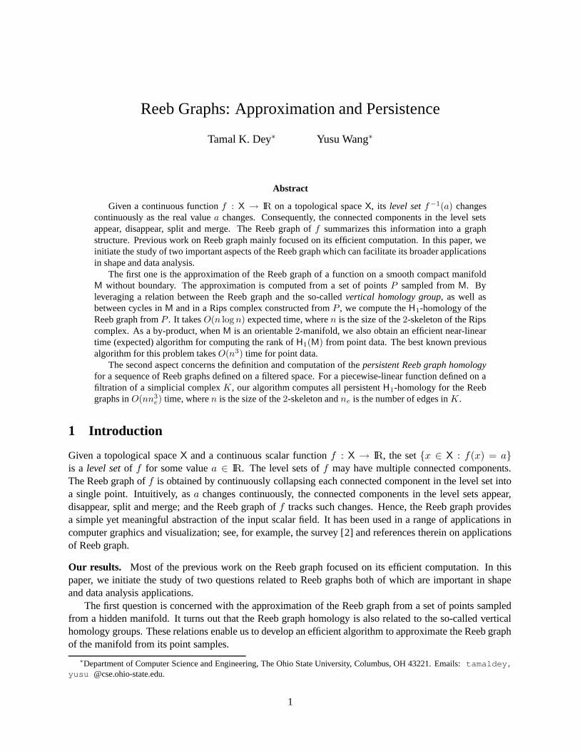
α1

α3

α2

We percolate the definitions from the homology classes to cycles. A cycle α is horizon-tal if [α], the standard homology class represented by α, is a horizontal class. Two cyclesα1 and α2 are vertically homologous if [α1] and [α2] are vertically homologous. Obviously,two p-cycles α1 and α2 are vertically homologous if and only if there is a (p + 1)-chain Bsuch that ∂B + α1 + α2 is a horizontal cycle. See the torus in the right figure for an ex-ample, where α2 is a horizontal cycle as it is homologous to α3 carried by a loop containedin a connected component of a level set; while α1 is a vertical cycle, i.e, [α1] is a verticalhomology class. We say that {α1, . . . , αk} is a set of base cycles for Hp(X) if {[α1], . . . , [αk]} form a basisfor Hp(X). A set of base cycles for Hp(X) and Hp(X) are defined analogously.

Finally, the range of a loop γ ⊆ X, denoted by range(γ), is the interval [minx∈γ f(x),maxx∈αf(x)].The height of this loop, height(γ), is simply the length of range(γ). We extend the definitions of rangeand height to cycles by saying that range(α) = range(γ) and height(α) = height(γ) where the cycleα ∈ Z1(X) is carried by the loop γ. The height of a homology class ω, denoted by height(ω), is theminimal height of any cycle in this class. Notice that the height of a horizontal class ω is not necessarilyzero since ω may be the addition of multiple height-0 horizontal classes.

Reeb graph. Given a triangulable topological space X and a continuous function f : X → IR, we say thattwo points x, y ∈ X are equivalent, denoted by x ∼ y, if and only if x and y belong to the same connected

3

component of Xa for some a ∈ IR. Consider the quotient space X∼, which is the set of equivalence classesequipped with the quotient topology induced by this equivalence relation; X∼ is also called the Reeb graphof X with respect to f , denoted by Rf (X). See Figure 1 (a) and (b) for an example.

f

c6

c5

c4

c3

c2

c1

µ

Xc3

Xc4

Xc × [0, 1]

X[c3,c4]Xc

(a) (b) (c)

Figure 1: (a) X is a solid torus and its Reeb graph w.r.t the height function f is shown in (b). (c) If f islevelset-tame, then there is a continuous map µ : Xc × [0, 1] → X[c3,c4] whose restriction to the open setXc × (0, 1) is a homeomorphism.

An alternative way to view the Reeb graph is that there is a natural continuous surjection Φ : X → X∼

where Φ(x) = Φ(y) if and only if x and y come from the same connected component of a level set off . In this sense, Rf (X) is obtained by continuously identifying each connected component. The map Φinduces a scalar function f : Rf (X) → IR where f(p) = f(x) if p = Φ(x). Since f(x) = f(y) wheneverΦ(x) = Φ(y), the function f is well-defined. Since f is continuous, so is f . The range or height of a loopin Rf (X) is measured with respect to this function f . In this paper, we abuse the notation slightly and use fto also refer to f for simplicity.

3 Reeb graphs and vertical homology

In this section, we show that H1(Rf (X)) and the first vertical homology group H1(X) of X are isomorphic1 .The surjection Φ : X → Rf (X) induces a chain map Φ# from the 1-chains of X to the 1-chains of Rf (X)

which eventually induces a homomorphism Φ∗ : H1(X) → H1(Rf (X)). For the horizontal subgroup H1(X),we have that Φ∗(H1(X)) = ∅ = H1(Rf (X)). Hence Φ∗ induces a well-defined homomorphism between thequotient groups

Φ : H1(X) =H1(X)

H1(X)→

H1(Rf (X))

H1(Rf (X))= H1(Rf (X)).

In what follows, we show that Φ is indeed an isomorphism under some mild conditions. Intuitively, this isnot surprising as Φ maps each contour in the level set to a single point, which in turn also collapses everyhorizontal cycle.

For technical reasons, we consider functions that behave nicely. Specifically, we call a continuousfunction f : X → IR levelset-tame if there are only finite number of discrete values {c1, . . . , cm} such thatthe following is true: for any two consecutive ci and ci+1, (i) there is a homeomorphism µi : Xc × (0, 1) →X(ci,ci+1) for an arbitrary c ∈ (ci, ci+1); (ii) the homeomorphism µi can be extended to a continuous mapµi : Xc × [0, 1] → X[ci,ci+1]; (iii) there is no map satisfying (i) and (ii) whose extension in (ii) is also ahomeomorphism. We call cis the levelset-critical values. See Figure 1 (c) for an example. It can be shown

1This relation is observed for 2-manifolds in [6], but to the best of our knowledge, it has not been formally introduced andproved anywhere yet for general topological spaces. We include it here for completion.

4

that Morse functions on a compact smooth manifold and piecewise-linear functions on a finite simplicialcomplex are both levelset-tame functions.

The set of points from Rf (X) having levelset-critical values are called the nodes of the Reeb graphRf (X). (Some nodes may have degree 2). Removing the nodes from Rf (X) leaves a set of connectedcomponents. The closure of each such component is an arc of Rf (X). Given an arc γ of Rf (X), let X(γ)denote the pre-images of γ under the map Φ. Observe that any two points of X(γ) are path-connected withinX(γ).

s1 s2

p1 q1

q2p2

s3

s

s1 s2

p1 q1

q2p2

s3

s

(b) (c)

s1 s2

(a)

p2 q2

p1 q1

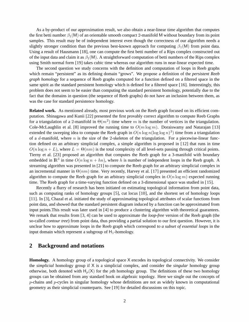
Figure 2: (a) An illustration of the cylinder C = S × [0, 1], where each horizontal slice of this cylinder isa copy of S. (b) s is the projection of s = s1 ◦ s3 ◦ s2 from the product space onto the slice C[1]. (c) Theboundary of the surface B ′ is s + s.

We now show two results to relate vertical cycles in X and cycles in Rf (X) for a levelset-tame functionf . Our main result of this section is obtained from these two claims.

Claim 3.1 Let f : X → IR be a levelset-tame function. Given a loop γ ⊆ Rf (X), there is a loop γ ⊆ X

such that Φ(γ) = γ and range(γ) = range(γ).

Proof: We construct γ from γ as follows: suppose γ consists of a sequences of k arcs

γ[p1, p2], γ[p2, p3], . . . , γ[pk, p1]

where each pi is a node of the Reeb graph Rf (X). For each pi, choose an arbitrary pre-image qi ∈ X fromΦ−1(pi). Now for each arc γ[pi, pi+1], connect qi and qi+1 within X(γ[pi, pi+1]) by γ[qi, qi+1] arbitrarily.The concatenation of all γ[qi, qi+1] provides γ ⊂ X. It is easy to check that range(γ) = range(γ).

Claim 3.2 Let f : X → IR be a levelset-tame function. For a 1-cycle α ∈ Z1(X) the image Φ#(α)represents a trivial class in H1(Rf (X)) if only if [α] is horizontal in H1(X).

Proof: First, if a cycle α is from a horizontal class [α], then there is another representative cycle α ′ of [α]such that the carrier of α′ is contained in a discrete set of level-sets. Since each connected component withina level-set is mapped to a single point in the Reeb graph, the image Φ#(α′) in Rf (X) is a 0-chain and thushas trivial H1-homology. It follows that Φ#(α) also has trivial homology.

We now show the opposite direction. That is, if the image of α in Rf (X) has trivial homology, then [α]must be horizontal. For simplicity, assume that Φ#(α) is carried by a sequence of full arcs in Rf (X). Thecase where Φ#(α) is carried by some arcs only partially can be handled similarly. Since Φ#(α) has trivialhomology in H1(Rf (X)), each arc of Rf (X) appears even number of times in its carrier. Consider an arc γof Rf (X) and its pre-image X(γ) in X. Let cp and cp+1 be the levelset-critical values of the endpoints of γ.Assume that the carrier of α consists of 2k pieces in X(γ), whose chains are α1, α2, . . . , α2k . Partition it intok pairs (α1, α2), . . . , (α2k−1, α2k). Consider an arbitrary pair (α2i, α2i+1). We now argue that there exists a2-chain Bi such that the carrier of ∂Bi +α2i +α2i+1 lies in the level sets Xcp ∪Xcp+1 . Notice that by taking

5

the union of all such Bis for i ∈ [1, k], we obtain a 2-chain Bγ such that the carrier of ∂Bγ +α1 + · · ·+α2k

is contained in the two level sets Xcp and Xcp+1 . Taking the union of Bγ for all arcs γ from Rf (X) gives riseto a 2-chain B such that the carrier of ∂B + α is contained in a discrete set of level sets. It follows that α isa horizontal cycle.

Now, we only need to focus on the construction of the 2-chain Bi for a pair of chains α2i and α2i+1.Let π1 and π2 be the two curves carrying α2i and α2i+1. Recall that there is a continuous map µ : Xc ×[0, 1] → X[cp,cp+1] for an arbitrary but fixed c ∈ (cp, cp+1), whose restriction to the open set Xc × (0, 1) isa homeomorphism onto X(cp,cp+1). Let π1

o and π2o denote the interiors of π1 and π2, respectively; π1

o andπ2

o have unique pre-images s1o and s2

o in Xc × (0, 1) under µ.The product space Xc × [0, 1] has several connected components each of which, called a cylinder, cor-

responds to the product between a connected component in the level-set Xc and [0, 1]. The images of allsuch cylinders under µ can touch each other only in Xcp or in Xcp+1 when µ is no longer a homeomorphism.See Figure 1 (c) for an illustration, where in this example, Xc × [0, 1] has three cylinders. The cylinder thatcontains s1

o and s2o is denoted as C = S × [0, 1], where S is the corresponding connected component in

Xc. Every point x ∈ C can be represented as x = (x, t), where x ∈ S is called its horizontal coordinate andt ∈ [0, 1] is its vertical coordinate (or height). A slice C[t] refers to one copy of S at height t.

Let s1 (resp. s2) denote the closure of s1o (resp. s2

o) in C, with p1 and p2 (resp. q1 and q2) being itsendpoints. See Figure 2 (a) for an illustration. Notice that µ(s1) = π1 and µ(s2) = π2 due to the continuityof µ. Since each slice C[t] of the cylinder C is path-connected, there is a path, say s3, that connects p1

and q1 in C[0]. Let s denote the concatenated curve s1 ◦ s3 ◦ s2; see Figure 2 (b). Now for every pointx = (x, tx) ∈ s, consider the “vertical line” lx = {(x, t) | t ∈ [tx, 1]}. That is, lx contains the images ofx in each slice C[t] with t ≥ tx. The union of lxs for all x ∈ s traces out a 2-dimensional surface B ′. Theboundary of B ′, denoted by bndB ′, is bndB′ = s ◦ s where s is the image of s in C[1]. See Figure 2 (b)and (c).

Finally, through the continuous map µ, we obtain a 2-chain Bi whose carrier is µ(B ′) ⊂ X[cp,cp+1] andbndµ(B′) = π1 ◦ µ(s3) ◦ π2 ◦ µ(s). Furthermore, µ(s3) ∪ µ(s) lie in the level-sets Xcp ∪ Xcp+1 . Asdescribed earlier, by taking the union of such 2-chains for all pairs and for all arcs, we obtain a 2-chainB whose boundary is exactly α and a finite set of cycles whose carriers are contained in a discrete set oflevel-sets

⋃cp

Xcp . Hence [α] must be a horizontal homology class.

Theorem 3.3 Given a levelset-tame function f : X → IR, let Φ : H1(X) → H1(Rf (X)) be the homo-morphism induced by the surjection Φ : X → Rf (X) as defined before. The map Φ is an isomorphism.Furthermore, for any vertical homology class ω ∈ H1(X), we have that height(ω) = height(Φ(ω)).

Proof: It follows from Claim 3.1 that the homomorphism Φ∗ : H1(X) → H1(Rf (X)) induced by Φ issurjective. Combining this with the fact that Φ∗(H1(X)) = ∅ = H1(Rf (X)) implies that the quotient map Φis also surjective. The injectivity of Φ follows from Claim 3.2. Hence Φ is an isomorphism.

For the second part of the theorem, suppose α is a vertical cycle such that [α] = ω and height(α) =height(ω), i.e., α is a thinnest cycle in the vertical homology class ω. Let γ ⊆ Rf (X) be the loop in Rf (X)that carries the cycle in the homology class Φ(ω) ∈ H1(Rf (X)). We have that

height(α) ≥ height(Φ#(α)) ≥ height(Φ(ω)) = height(γ) (1)

On the other hand, by Claim 3.1, there is a loop γ ⊆ X such that Φ(γ) = γ and height(γ) = height(γ).Let α be any 1-cycle carried by γ. By Claim 3.2, we have [α] = ω, as the cycle α + α is mapped to atrivial cycle in Rf (X). Hence height(γ) = height(γ) ≥ height(α). Combining this with Eqn (1) provesthat height(Φ(ω)) = height(ω).

6

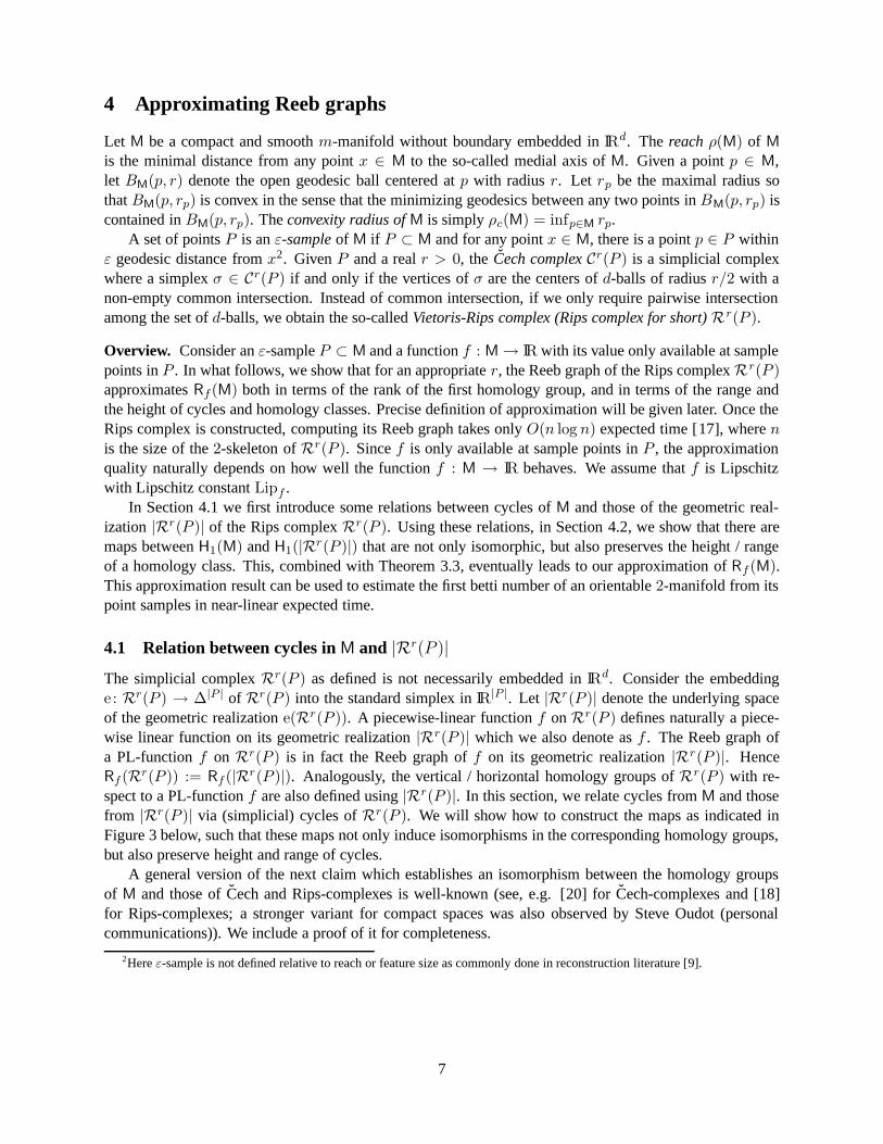
4 Approximating Reeb graphs

Let M be a compact and smooth m-manifold without boundary embedded in IRd. The reach ρ(M) of M

is the minimal distance from any point x ∈ M to the so-called medial axis of M. Given a point p ∈ M,let BM(p, r) denote the open geodesic ball centered at p with radius r. Let rp be the maximal radius sothat BM(p, rp) is convex in the sense that the minimizing geodesics between any two points in BM(p, rp) iscontained in BM(p, rp). The convexity radius of M is simply ρc(M) = infp∈M rp.

A set of points P is an ε-sample of M if P ⊂ M and for any point x ∈ M, there is a point p ∈ P withinε geodesic distance from x2. Given P and a real r > 0, the Cech complex Cr(P ) is a simplicial complexwhere a simplex σ ∈ Cr(P ) if and only if the vertices of σ are the centers of d-balls of radius r/2 with anon-empty common intersection. Instead of common intersection, if we only require pairwise intersectionamong the set of d-balls, we obtain the so-called Vietoris-Rips complex (Rips complex for short) Rr(P ).

Overview. Consider an ε-sample P ⊂ M and a function f : M → IR with its value only available at samplepoints in P . In what follows, we show that for an appropriate r, the Reeb graph of the Rips complex Rr(P )approximates Rf (M) both in terms of the rank of the first homology group, and in terms of the range andthe height of cycles and homology classes. Precise definition of approximation will be given later. Once theRips complex is constructed, computing its Reeb graph takes only O(n log n) expected time [17], where nis the size of the 2-skeleton of Rr(P ). Since f is only available at sample points in P , the approximationquality naturally depends on how well the function f : M → IR behaves. We assume that f is Lipschitzwith Lipschitz constant Lipf .

In Section 4.1 we first introduce some relations between cycles of M and those of the geometric real-ization |Rr(P )| of the Rips complex Rr(P ). Using these relations, in Section 4.2, we show that there aremaps between H1(M) and H1(|R

r(P )|) that are not only isomorphic, but also preserves the height / rangeof a homology class. This, combined with Theorem 3.3, eventually leads to our approximation of Rf (M).This approximation result can be used to estimate the first betti number of an orientable 2-manifold from itspoint samples in near-linear expected time.

4.1 Relation between cycles in M and |Rr(P )|

The simplicial complex Rr(P ) as defined is not necessarily embedded in IRd. Consider the embeddinge : Rr(P ) → ∆|P | of Rr(P ) into the standard simplex in IR|P |. Let |Rr(P )| denote the underlying spaceof the geometric realization e(Rr(P )). A piecewise-linear function f on Rr(P ) defines naturally a piece-wise linear function on its geometric realization |Rr(P )| which we also denote as f . The Reeb graph ofa PL-function f on Rr(P ) is in fact the Reeb graph of f on its geometric realization |Rr(P )|. HenceRf (Rr(P )) := Rf (|Rr(P )|). Analogously, the vertical / horizontal homology groups of Rr(P ) with re-spect to a PL-function f are also defined using |Rr(P )|. In this section, we relate cycles from M and thosefrom |Rr(P )| via (simplicial) cycles of Rr(P ). We will show how to construct the maps as indicated inFigure 3 below, such that these maps not only induce isomorphisms in the corresponding homology groups,but also preserve height and range of cycles.

A general version of the next claim which establishes an isomorphism between the homology groupsof M and those of Cech and Rips-complexes is well-known (see, e.g. [20] for Cech-complexes and [18]for Rips-complexes; a stronger variant for compact spaces was also observed by Steve Oudot (personalcommunications)). We include a proof of it for completeness.

2Here ε-sample is not defined relative to reach or feature size as commonly done in reconstruction literature [9].

7

Z1(M)d //

µ = e#◦d

++

Z1(Rr(P ))

h#

oo

e#//Z1(|R

r(P )|)g

oo

ξ = h#◦g

kk

Figure 3: Maps between cycle groups

Claim 4.1 Let P ⊂ M be an ε-sample and r a parameter such that 4ε ≤ r ≤ 12

√35ρ(M). Then,

H1(Cr(P )) ≈ H1(R

r(P )) ≈ H1(C2r(P )) ≈ H1(M).

The first two isomorphisms are induced by the natural inclusion from C r(P ) to Rr(P ) and then to C2r(P ).The last isomorphism is induced by the homotopy equivalence defined in Proposition 3.3 of [11].

Proof: Consider the following sequence of inclusions:

Cr(P )i1↪→ Rr(P )

i2↪→ C2r(P )

i3↪→ R2r(P )

i4↪→ C4r(P ).

Let i∗ : H1(Rr(P )) → H1(R

2r(P )) be induced by the inclusion i = i3 ◦ i2. By Proposition 3.4 [11], wehave that image(i∗) ≈ H1(C

r(P )).Notice that since C2r(P ) and R2r(P ) share the same edge set, and R2r(P ) only has more triangles than

C2r(P ), the inclusion induces a surjection from H1(C2r(P )) to H1(R

2r(P )). Combining this with the factthat image(i∗) ≈ H1(C

r) ≈ H1(M) ≈ H1(C2r(P )), one obtains that exactly rank(H1(C

2r(P ))) number ofindependent homology classes survive from H1(R

r(P )) to H1(R2r(P )) through H1(C

2r(P )) via inclusions.Hence we have H1(C

2r(P )) ≈ H1(R2r(P )) where the isomorphism is induced by inclusion. By a similar

argument we also have that H1(Cr(P )) ≈ H1(R

r(P )) and the isomorphism is also induced by inclusion.Since H1(C

r(P )) ≈ H1(C2r(P )), we have H1(C

r(P )) ≈ H1(Rr(P )) ≈ H1(C

2r(P )) ≈ H1(R2r(P )), and

all the isomorphisms are induced by inclusions.

Maps d and h#. We now define maps as indicated in Figure 3. First, given a cycle α ∈ Z1(M), we map itto a cycle d(α) ∈ Z1(R

r(P )) using the same Decomposition method [1] as applied in [11]. In particular,break the carrier of α into pieces where each piece has length at most r − 2ε. For each piece with endpointsxi and xi+1, find the closest sample points pi and pi+1 from P to xi and xi+1, respectively, and connect pi

and pi+1 (which is necessarily an edge in Rr(P ) by triangle inequality). The resulting simplicial 1-cycle inRr(P ) is d(α).

We now define the map h : Rr(P ) → M as the inclusion map Rr(P ) ↪→ C2r(P ) composed withthe homotopy equivalence from C2r(P ) to M introduced in Proposition 3.3 of [11]. The correspondingchain map h# maps p-cycles to p-cycles, and p-boundaries to p-boundaries inducing the homomorphismh∗ : Hp(R

r(P )) → Hp(M). We restrict h∗ only to the first homology group h∗ : H1(Rr(P )) → H1(M).

By Claim 4.1, h∗ is an isomorphism.The following lemma states that d: Z1(M) → Z1(R

r(P )) is in fact the homology-inverse of h#, whicheventually implies that the map d takes homologous cycles to homologous cycles and induces a well-definedhomomorphism (in fact, an isomorphism) d∗ : H1(M) → H1(R

r(P )). The ranges of mapped cycles are alsorelated. We put the proof of the following lemma in Appendix A to maintain the flow of the presentation.Given two intervals I1 = [a, b] and I2 = [c, d], we say that I1 is oneside-δ-close to I2 if: [a, b] ⊆ [c−δ, d+δ].I1 and I2 are δ-Hausdorff-close if the two intervals are oneside-δ-close to each other. In the Lemma below,

8

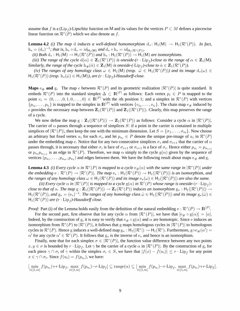
assume that f is a (Lipf )-Lipschitz function on M and its values for the vertices P ⊂ M defines a piecewiselinear function on Rr(P ) which we also denote as f .

Lemma 4.2 (i) The map d induces a well-defined homomorphism d∗ : H1(M) → H1(Rr(P )). In fact,

h∗ = (d∗)−1; that is, h∗ ◦ d∗ = idH1(M) and d∗ ◦ h∗ = idH1(Rr(P )).

(ii) Both d∗ : H1(M) → H1(Rr(P )) and h∗ : H1(R

r(P )) → H1(M) are isomorphisms.(iii) The range of the cycle d(α) ∈ Z1(R

r(P )) is oneside-(r · Lipf )-close to the range of α ∈ Z1(M).Similarly, the range of the cycle h#(α) ∈ Z1(M) is oneside-(·Lipf )-close to α ∈ Z1(R

r(P )).(iv) The ranges of any homology class ω ∈ H1(M) (resp. ω ∈ H1(Rr(P ))) and its image d∗(ω) ∈

H1(Rr(P )) (resp. h∗(ω) ∈ H1(M)), are (r · Lipf )-Hausdorff-close.

Maps e# and g. The map e between Rr(P ) and its geometric realization |Rr(P )| is quite standard. Itembeds Rr(P ) into the standard simplex ∆ ⊂ IR|P | as follows: Each vertex pi ∈ P is mapped to thepoint vi = (0, . . . , 0, 1, 0, . . . , 0) ∈ IR|P | with the ith position 1; and a simplex in Rr(P ) with vertices{pi0 , . . . , pil} is mapped to the simplex in IR|P | with vertices {vi0 , . . . , vil}. The chain map e# induced bye provides the necessary map between Z1(R

r(P )) and Z1(|Rr(P )|). Clearly, this map preserves the range

of a cycle.We now define the map g : Z1(|R

r(P )|) → Z1(Rr(P )) as follows: Consider a cycle α in |Rr(P )|.

The carrier of α passes through a sequence of simplices S: if a point in the carrier is contained in multiplesimplices of |Rr(P )|, then keep the one with the minimum dimension. Let S = {σ1, . . . , σm}. Now choosean arbitrary but fixed vertex ui for each σi, and let pui

∈ P denote the unique pre-image of ui in Rr(P )under the embedding map e. Notice that for any two consecutive simplices σi and σi+1 that the carrier of αpasses through, it is necessary that either σi is face of σi+1 or σi+1 is a face of σi. Hence either pui

= pui+1

or puipui+1 is an edge in Rr(P ). Therefore, we map α simply to the cycle g(α) given by the sequence of

vertices (pu1 , . . . , pum , pu1) and edges between them. We have the following result about maps e# and g.

Lemma 4.3 (i) Every cycle α in Rr(P ) is mapped to a cycle e#(α) with the same range in |Rr(P )| underthe embedding e : Rr(P ) → |Rr(P )|. The map e∗ : H1(R

r(P )) → H1(|Rr(P )|) is an isomorphism, and

the ranges of any homology class ω ∈ H1(Rr(P )) and its image e∗(ω) ∈ H1(|R

r(P )|) are also the same.(ii) Every cycle α in |Rr(P )| is mapped to a cycle g(α) in Rr(P ) whose range is oneside-(r · Lipf )-

close to that of α. The map g : Z1(|Rr(P )|) → Z1(R

r(P )) induces an isomorphism g∗ : H1(|Rr(P )|) →

H1(Rr(P )), and g∗ = (e∗)

−1. The ranges of any homology class ω ∈ H1(|Rr(P )|) and its image g∗(ω) ∈

H1(Rr(P )) are (r · Lipf )-Hausdorff close.

Proof: Part (i) of the Lemma holds easily from the definition of the natural embedding e : Rr(P ) → IR|P |.For the second part, first observe that for any cycle α from |Rr(P )|, we have that [e# ◦ g(α)] = [α].

Indeed, by the construction of g, it is easy to verify that e# ◦ g(α) and α are homotopic. Since e induces anisomorphism from Rr(P ) to |Rr(P )|, it follows that g maps homologous cycles in |Rr(P )| to homologouscycles in Rr(P ). Hence g induces a well-defined map g∗ : H1(|R

r|) → H1(Rr). Furthermore, g◦e#(α′) =

α′ for any cycle α′ ∈ Rr(P ). It follows that g∗ is the inverse of e∗ and hence is an isomorphism.Finally, note that for each simplex σ ∈ |Rr(P )|, the function value difference between any two points

x, y ∈ σ is bounded by r · Lipf . Let γ be the carrier of a cycle α in |Rr(P )|. By the construction of g, foreach piece γ ∩ σi of γ within the simplex σi ∈ S, we have that |f(x) − f(ui)| ≤ r · Lipf for any pointx ∈ γ ∩ σi. Since f(ui) = f(pui

), we have:

[ mini∈[1,m]

f(pui)+r·Lipf , max

i∈[1,m]f(pui

)−r·Lipf ] ⊆ range(α) ⊆ [ mini∈[1,m]

f(pui)−r·Lipf , max

i∈[1,m]f(pui

)+r·Lipf ].

9

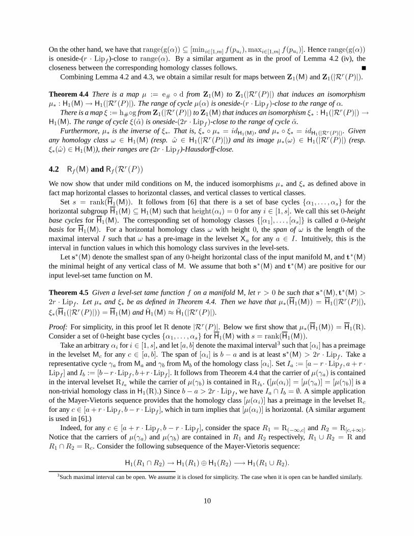
On the other hand, we have that range(g(α)) ⊆ [mini∈[1,m] f(pui),maxi∈[1,m] f(pui

)]. Hence range(g(α))is oneside-(r · Lipf )-close to range(α). By a similar argument as in the proof of Lemma 4.2 (iv), thecloseness between the corresponding homology classes follows.

Combining Lemma 4.2 and 4.3, we obtain a similar result for maps between Z1(M) and Z1(|Rr(P )|).

Theorem 4.4 There is a map µ := e# ◦ d from Z1(M) to Z1(|Rr(P )|) that induces an isomorphism

µ∗ : H1(M) → H1(|Rr(P )|). The range of cycle µ(α) is oneside-(r · Lipf )-close to the range of α.

There is a map ξ := h#◦g from Z1(|Rr(P )|) to Z1(M) that induces an isomorphism ξ∗ : H1(|R

r(P )|) →H1(M). The range of cycle ξ(α) is oneside-(2r · Lipf )-close to the range of cycle α.

Furthermore, µ∗ is the inverse of ξ∗. That is, ξ∗ ◦ µ∗ = idH1(M), and µ∗ ◦ ξ∗ = idH1(|Rr(P )|). Givenany homology class ω ∈ H1(M) (resp. ω ∈ H1(|R

r(P )|)) and its image µ∗(ω) ∈ H1(|Rr(P )|) (resp.

ξ∗(ω) ∈ H1(M)), their ranges are (2r · Lipf )-Hausdorff-close.

4.2 Rf(M) and Rf(Rr(P ))

We now show that under mild conditions on M, the induced isomorphisms µ∗ and ξ∗ as defined above infact map horizontal classes to horizontal classes, and vertical classes to vertical classes.

Set s = rank(H1(M)). It follows from [6] that there is a set of base cycles {α1, . . . , αs} for thehorizontal subgroup H1(M) ⊆ H1(M) such that height(αi) = 0 for any i ∈ [1, s]. We call this set 0-heightbase cycles for H1(M). The corresponding set of homology classes {[α1], . . . , [αs]} is called a 0-heightbasis for H1(M). For a horizontal homology class ω with height 0, the span of ω is the length of themaximal interval I such that ω has a pre-image in the levelset Xa for any a ∈ I . Intuitively, this is theinterval in function values in which this homology class survives in the level-sets.

Let s∗(M) denote the smallest span of any 0-height horizontal class of the input manifold M, and t∗(M)

the minimal height of any vertical class of M. We assume that both s∗(M) and t

∗(M) are positive for ourinput level-set tame function on M.

Theorem 4.5 Given a level-set tame function f on a manifold M, let r > 0 be such that s∗(M), t∗(M) >

2r · Lipf . Let µ∗ and ξ∗ be as defined in Theorem 4.4. Then we have that µ∗(H1(M)) = H1(|Rr(P )|),

ξ∗(H1(|Rr(P )|)) = H1(M) and H1(M) ≈ H1(|R

r(P )|).

Proof: For simplicity, in this proof let R denote |Rr(P )|. Below we first show that µ∗(H1(M)) = H1(R).Consider a set of 0-height base cycles {α1, . . . , αs} for H1(M) with s = rank(H1(M)).

Take an arbitrary αi for i ∈ [1, s], and let [a, b] denote the maximal interval3 such that [αi] has a preimagein the levelset Mc for any c ∈ [a, b]. The span of [αi] is b − a and is at least s

∗(M) > 2r · Lipf . Take arepresentative cycle γa from Ma and γb from Mb of the homology class [αi]. Set Ia := [a− r · Lipf , a + r ·Lipf ] and Ib := [b−r ·Lipf , b+r ·Lipf ]. It follows from Theorem 4.4 that the carrier of µ(γa) is containedin the interval levelset RIa while the carrier of µ(γb) is contained in RIb

. ([µ(αi)] = [µ(γa)] = [µ(γb)] is anon-trivial homology class in H1(R).) Since b − a > 2r · Lipf , we have Ia ∩ Ib = ∅. A simple applicationof the Mayer-Vietoris sequence provides that the homology class [µ(αi)] has a preimage in the levelset Rc

for any c ∈ [a + r ·Lipf , b− r · Lipf ], which in turn implies that [µ(αi)] is horizontal. (A similar argumentis used in [6].)

Indeed, for any c ∈ [a + r · Lipf , b − r · Lipf ], consider the space R1 = R(−∞,c] and R2 = R[c,+∞).Notice that the carriers of µ(γa) and µ(γb) are contained in R1 and R2 respectively, R1 ∪ R2 = R andR1 ∩ R2 = Rc. Consider the following subsequence of the Mayer-Vietoris sequence:

H1(R1 ∩ R2) → H1(R1) ⊕ H1(R2) −→ H1(R1 ∪ R2).

3Such maximal interval can be open. We assume it is closed for simplicity. The case when it is open can be handled similarly.

10

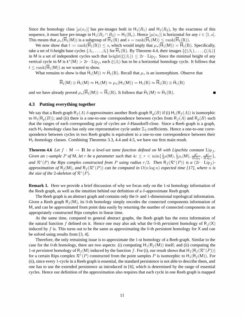
Since the homology class [µ(αi)] has pre-images both in H1(R1) and H1(R2), by the exactness of thissequence, it must have pre-image in H1(R1 ∩R2) = H1(Rc). Hence [µ(αi)] is horizontal for any i ∈ [1, s].This means that µ∗(H1(M)) is a subgroup of H1(R) and s = rank(H1(M)) ≤ rank(H1(R)).

We now show that t := rank(H1(R)) ≤ s, which would imply that µ∗(H1(M)) = H1(R). Specifically,take a set of 0-height base cycles {β1, . . . , βt} for H1(R). By Theorem 4.4, their images {ξ(β1), . . . , ξ(βt)}in M is a set of independent cycles such that height(ξ(βi)) ≤ 2r · Lipf . Since the minimal height of anyvertical cycle in M is t

∗(M) > 2r · Lipf , each ξ(βi) has to be a horizontal homology cycle. It follows thatt ≤ rank(H1(M)) as we wanted to show.

What remains to show is that H1(M)) ≈ H1(R). Recall that µ∗ is an isomorphism. Observe that

H1(M) ⊕ H1(M) ≈ H1(M) ≈ µ∗(H1(M)) = H1(R) ≈ H1(R) ⊕ H1(R)

and we have already proved µ∗(H1(M)) = H1(R). It follows that H1(M) ≈ H1(R).

4.3 Putting everything together

We say that a Reeb graph Rf (A) δ-approximates another Reeb graph Rg(B) if (i) H1(Rf (A)) is isomorphicto H1(Rg(B)); and (ii) there is a one-to-one correspondence between cycles from Rf (A) and Rg(B) suchthat the ranges of each corresponding pair of cycles are δ-Hausdorff-close. Since a Reeb graph is a graph,each H1-homology class has only one representative cycle under Z2 coefficients. Hence a one-to-one corre-spondence between cycles in two Reeb graphs is equivalent to a one-to-one correspondence between theirH1-homology classes. Combining Theorems 3.3, 4.4 and 4.5, we have our first main result.

Theorem 4.6 Let f : M → IR be a level-set tame function defined on M with Lipschitz constant Lipf .

Given an ε-sample P of M, let r be a parameter such that 4ε ≤ r < min{ 14ρ(M), 1

4ρc(M), t∗

2Lipf, s

∗

2Lipf},

and Rr(P ) the Rips complex constructed from P using radius r/2. Then Rf (Rr(P )) is a (2r · Lipf )-approximation of Rf (M), and Rf (Rr(P )) can be computed in O(n log n) expected time [17], where n isthe size of the 2-skeleton of Rr(P ).

Remark 1. Here we provide a brief discussion of why we focus only on the 1-st homology information ofthe Reeb graph, as well as the intuition behind our definition of a δ-approximate Reeb graph.

The Reeb graph is an abstract graph and contains only the 0- and 1-dimensional topological information.Given a Reeb graph Rf (M), its 0-th homology simply encodes the connected components information ofM, and can be approximated from point data easily by returning the number of connected components in anappropriately constructed Rips complex in linear time.

At the same time, compared to general abstract graphs, the Reeb graph has the extra information ofthe natural function f defined on it. Hence one may also ask what the 0-th persistent homology of Rf (X)induced by f is. This turns out to be the same as approximating the 0-th persistent homology for X and canbe solved using results from [3, 4].

Therefore, the only remaining issue is to approximate the 1-st homology of a Reeb graph. Similar to thecase for the 0-th homology, there are two aspects: (i) computing H1(Rf (M)) itself; and (ii) computing the1-st persistent homology of Rf (M) induced by the function f . For (i), our result shows that H1(Rf (Rr(P )))for a certain Rips complex Rr(P ) constructed from the point samples P is isomorphic to H1(Rf (M)). For(ii), since every 1-cycle in a Reeb graph is essential, the standard persistence is not able to describe them, andone has to use the extended persistence as introduced in [6], which is determined by the range of essentialcycles. Hence our definition of the approximation also requires that each cycle in one Reeb graph is mapped

11

uniquely to a cycle in the other one such that the ranges of these two cycles are close.

Remark 2. One can strengthen Theorem 4.6 slightly to show that if the parameter r does not satisfy theconditions that r < t

∗

2Lipfor r < s

∗

2Lipf, then all homology classes of H1(Rf (M)) with height at least

2r · Lipf are preserved in H1(Rf (Rr(P ))) (and vice versa).

Computing β1(M) for orientable 2-manifolds. It was shown in [8] that for a Morse function f : M → IRdefined on a compact orientable surface M without boundary, one has rank(H1(M)) = 2·rank(H1(Rf (M))).Hence intuitively, using Theorem 4.6, we can compute β1(M) = rank(H1(M)) by 2 · rank(H1(Rf (Rr(P )))from an appropriate f and a Rips Complex Rr(P ) constructed from a point sample P of M. Specifically,choose a function f : M → IR so that we can evaluate it at points in P . For example, pick a base pointv ∈ P and define a function fv(x) to be the Euclidean distance from x ∈ M to the base point v. Observethat the Lipschitz constant of this function fv is at most 1. Our algorithm simply computes the Reeb graphRfv(Rr(P )) and returns 2 · rank(H1(Rfv(Rr(P ))).

Corollary 4.7 Let M be an orientable smooth compact 2-manifold M without boundary and P an ε-sampleof M. The above algorithm computes β1(M)) in O(n log n) expected time if t

∗(M) and s∗(M) are positive

for the chosen function f , and the parameters satisfy 4ε ≤ r < min{ 14ρ(M), 1

4ρc(M), t∗

2Lipf, s

∗

2Lipf}.

Observe that a Morse function on an orientable 2-manifold provides positive t∗ and s

∗. We remark thatour algorithm produces a correct answer only under good choices of f and r; while previously, the bestalgorithm to estimate β1(M) only depends on choosing r small enough. The advantage of our algorithm isits efficiency, as the previous algorithm needs to compute the first-betti number of the simplicial complexRr(P ), which takes O(n3) time no matter what the intrinsic dimension of M is.

5 Persistent Reeb graph

Imagine that we have a set of points P sampled from a hidden space X, and f : X → IR a function whosevalues at points in P are available. We wish to study this function f through its Reeb graph. A naturalapproach to approximate X from P is to construct a Rips complex Rr(P ) from P . Since it is often unclearwhat the right value of r should be, it is desirable to compute a series of Reeb graphs from Rips complexesconstructed with various r, and then find out which cycles in the Reeb graph persist. This calls for computingpersistent homology groups for the sequence of Reeb graphs.

Let K1 ⊆ K2 ⊆ · · · ⊆ Kn be a filtration of a simplicial complex Kn. A piecewise linear functionf : |Kn| → IR provides a PL-function for every Ki, i ∈ [1, n]. Let Rf (Ki) denote the Reeb graph of fdefined on the geometric realization |Ki| of Ki and let Ri := Rf (Ki). Below we first show that there is asequence of homomorphisms H1(Ri) → H1(Ri+1) induced by the inclusions Ki ⊂ Ki+1. We then presentan algorithm to compute the persistent homologies induced by these homomorphisms.

5.1 Persistent Reeb graph homology

Let Φi denote the surjection from |Ki| → Ri, for any i ∈ [1, n]. The maps Φis, along with inclusionsbetween Kjs, induce a well-defined continuous map ξ : Ri → Rj , for any i < j. Indeed, given a pointp ∈ Ri, points in its pre-image Φ−1

i (p) come from the same contour in |Ki| and share the same functionvalue. Under inclusion |Ki| → |Kj | for any j > i, points in Φ−1

i (p) are still contained in a single contourin |Kj |. Thus all points in the pre-image Φ−1

i (p) are mapped to a single point ξ(p) ∈ Rj , implying that ξ iswell-defined. Let ιi denote the inclusion map from |Ki| to |Kj |, and ξi the induced map from Ri to Ri+1.We have the following diagram that commutes.

12

|K1|ι1 //

Φ1��

|K2|ι2 //

Φ2��

· · · · · ·ιn−1 // |Kn|

Φn��

R1ξ1 // R2

ξ2 // · · · · · ·ξn−1 // Rn

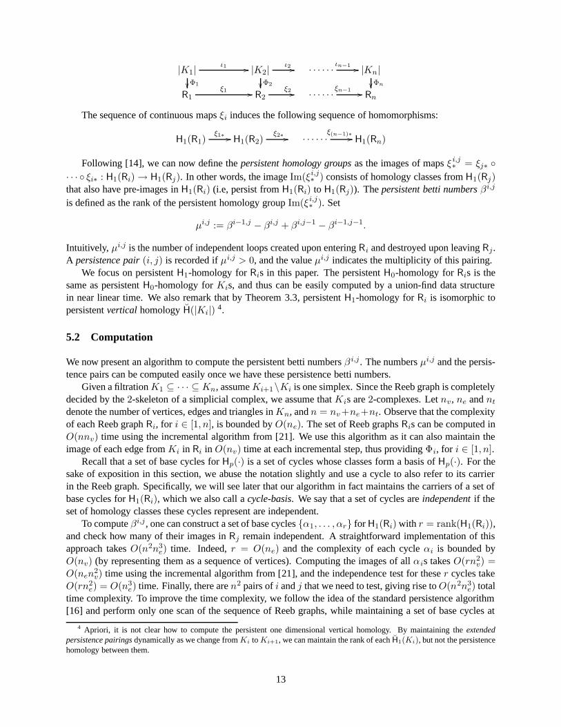
The sequence of continuous maps ξi induces the following sequence of homomorphisms:

H1(R1)ξ1∗ // H1(R2)

ξ2∗ // · · · · · ·ξ(n−1)∗

// H1(Rn)

Following [14], we can now define the persistent homology groups as the images of maps ξ i,j∗ = ξj∗ ◦

· · · ◦ ξi∗ : H1(Ri) → H1(Rj). In other words, the image Im(ξi,j∗ ) consists of homology classes from H1(Rj)

that also have pre-images in H1(Ri) (i.e, persist from H1(Ri) to H1(Rj)). The persistent betti numbers β i,j

is defined as the rank of the persistent homology group Im(ξ i,j∗ ). Set

µi,j := βi−1,j − βi,j + βi,j−1 − βi−1,j−1.

Intuitively, µi,j is the number of independent loops created upon entering Ri and destroyed upon leaving Rj .A persistence pair (i, j) is recorded if µi,j > 0, and the value µi,j indicates the multiplicity of this pairing.

We focus on persistent H1-homology for Ris in this paper. The persistent H0-homology for Ris is thesame as persistent H0-homology for Kis, and thus can be easily computed by a union-find data structurein near linear time. We also remark that by Theorem 3.3, persistent H1-homology for Ri is isomorphic topersistent vertical homology H(|Ki|)

4.

5.2 Computation

We now present an algorithm to compute the persistent betti numbers β i,j . The numbers µi,j and the persis-tence pairs can be computed easily once we have these persistence betti numbers.

Given a filtration K1 ⊆ · · · ⊆ Kn, assume Ki+1\Ki is one simplex. Since the Reeb graph is completelydecided by the 2-skeleton of a simplicial complex, we assume that Kis are 2-complexes. Let nv , ne and nt

denote the number of vertices, edges and triangles in Kn, and n = nv+ne+nt. Observe that the complexityof each Reeb graph Ri, for i ∈ [1, n], is bounded by O(ne). The set of Reeb graphs Ris can be computed inO(nnv) time using the incremental algorithm from [21]. We use this algorithm as it can also maintain theimage of each edge from Ki in Ri in O(nv) time at each incremental step, thus providing Φi, for i ∈ [1, n].

Recall that a set of base cycles for Hp(·) is a set of cycles whose classes form a basis of Hp(·). For thesake of exposition in this section, we abuse the notation slightly and use a cycle to also refer to its carrierin the Reeb graph. Specifically, we will see later that our algorithm in fact maintains the carriers of a set ofbase cycles for H1(Ri), which we also call a cycle-basis. We say that a set of cycles are independent if theset of homology classes these cycles represent are independent.

To compute βi,j , one can construct a set of base cycles {α1, . . . , αr} for H1(Ri) with r = rank(H1(Ri)),and check how many of their images in Rj remain independent. A straightforward implementation of thisapproach takes O(n2n3

e) time. Indeed, r = O(ne) and the complexity of each cycle αi is bounded byO(nv) (by representing them as a sequence of vertices). Computing the images of all αis takes O(rn2

v) =O(nen

2v) time using the incremental algorithm from [21], and the independence test for these r cycles take

O(rn2e) = O(n3

e) time. Finally, there are n2 pairs of i and j that we need to test, giving rise to O(n2n3e) total

time complexity. To improve the time complexity, we follow the idea of the standard persistence algorithm[16] and perform only one scan of the sequence of Reeb graphs, while maintaining a set of base cycles at

4 Apriori, it is not clear how to compute the persistent one dimensional vertical homology. By maintaining the extendedpersistence pairings dynamically as we change from Ki to Ki+1, we can maintain the rank of each H1(Ki), but not the persistencehomology between them.

13

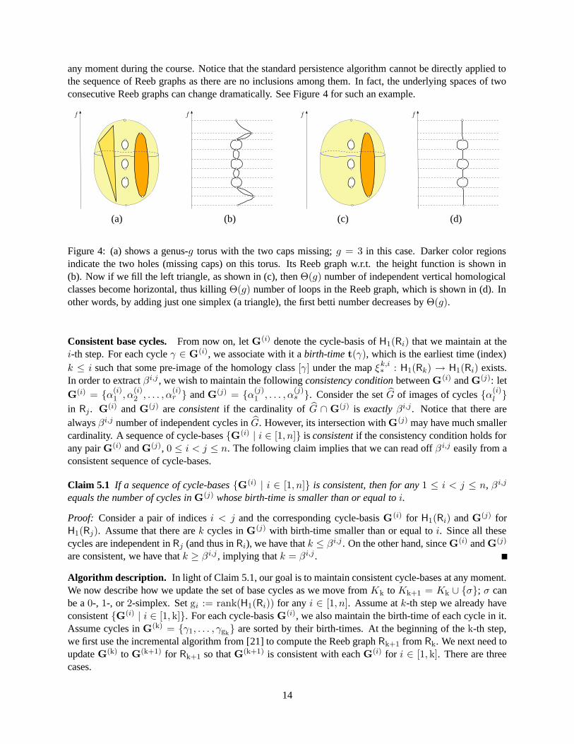
any moment during the course. Notice that the standard persistence algorithm cannot be directly applied tothe sequence of Reeb graphs as there are no inclusions among them. In fact, the underlying spaces of twoconsecutive Reeb graphs can change dramatically. See Figure 4 for such an example.

f f f f

(a) (b) (c) (d)

Figure 4: (a) shows a genus-g torus with the two caps missing; g = 3 in this case. Darker color regionsindicate the two holes (missing caps) on this torus. Its Reeb graph w.r.t. the height function is shown in(b). Now if we fill the left triangle, as shown in (c), then Θ(g) number of independent vertical homologicalclasses become horizontal, thus killing Θ(g) number of loops in the Reeb graph, which is shown in (d). Inother words, by adding just one simplex (a triangle), the first betti number decreases by Θ(g).

Consistent base cycles. From now on, let G(i) denote the cycle-basis of H1(Ri) that we maintain at the

i-th step. For each cycle γ ∈ G(i), we associate with it a birth-time t(γ), which is the earliest time (index)

k ≤ i such that some pre-image of the homology class [γ] under the map ξk,i∗ : H1(Rk) → H1(Ri) exists.

In order to extract βi,j , we wish to maintain the following consistency condition between G(i) and G

(j): letG

(i) = {α(i)1 , α

(i)2 , . . . , α

(i)r } and G

(j) = {α(j)1 , . . . , α

(j)s }. Consider the set G of images of cycles {α

(i)l }

in Rj . G(i) and G

(j) are consistent if the cardinality of G ∩ G(j) is exactly βi,j . Notice that there are

always βi,j number of independent cycles in G. However, its intersection with G(j) may have much smaller

cardinality. A sequence of cycle-bases {G(i) | i ∈ [1, n]} is consistent if the consistency condition holds forany pair G

(i) and G(j), 0 ≤ i < j ≤ n. The following claim implies that we can read off β i,j easily from a

consistent sequence of cycle-bases.

Claim 5.1 If a sequence of cycle-bases {G(i) | i ∈ [1, n]} is consistent, then for any 1 ≤ i < j ≤ n, β i,j

equals the number of cycles in G(j) whose birth-time is smaller than or equal to i.

Proof: Consider a pair of indices i < j and the corresponding cycle-basis G(i) for H1(Ri) and G

(j) forH1(Rj). Assume that there are k cycles in G

(j) with birth-time smaller than or equal to i. Since all thesecycles are independent in Rj (and thus in Ri), we have that k ≤ βi,j . On the other hand, since G

(i) and G(j)

are consistent, we have that k ≥ β i,j , implying that k = βi,j .

Algorithm description. In light of Claim 5.1, our goal is to maintain consistent cycle-bases at any moment.We now describe how we update the set of base cycles as we move from Kk to Kk+1 = Kk ∪ {σ}; σ canbe a 0-, 1-, or 2-simplex. Set gi := rank(H1(Ri)) for any i ∈ [1, n]. Assume at k-th step we already haveconsistent {G(i) | i ∈ [1, k]}. For each cycle-basis G

(i), we also maintain the birth-time of each cycle in it.Assume cycles in G

(k) = {γ1, . . . , γgk} are sorted by their birth-times. At the beginning of the k-th step,

we first use the incremental algorithm from [21] to compute the Reeb graph Rk+1 from Rk. We next need toupdate G

(k) to G(k+1) for Rk+1 so that G

(k+1) is consistent with each G(i) for i ∈ [1, k]. There are three

cases.

14

Case 1: σ is a vertex. A new connected component is created in Kk+1, consisting of only σ. Similarly,a new node is created in Rk+1. The set of base 1-cycles are not affected, and G

(k+1) = G(k).

Case 2: σ = pq is an edge. Let p = Φk(p) and q = Φk(q) be the images of endpoints p and q of σ inthe Reeb graph Rk. Adding σ to Kk creates a new edge e = pq in Rk+1. If p and q are not in the sameconnected component in Rk, then adding e will only reduce the rank of H0(Rk) by 1 and does not affectH1(Rk). In that case G

(k+1) = G(k). Otherwise, p and q are already connected in Rk. Adding e results in

rank(H1(Rk+1)) = rank(H1(Rk)) + 1. Let γ be any cycle in Rk+1 that contains e (which can be computedeasily in linear time). All previous base cycles in G

(k) will remain independent in Rk+1, and we simply setG

(k+1) = G(k) ∪ {γ}. The birth-time for γ is k + 1.

Case 3: σ is a triangle. The first two cases are simple and similar to the cases of standard persistencealgorithm. Case 3 is much more complicated. In particular, unlike the standard persistence algorithmwherein adding a triangle may reduce β1 by at most 1, the rank of H1(Rk) may decrease by Θ(gk). Whathappens is that even though β1(Kk) reduces by at most 1, arbitrary number of vertical homology classescan be converted into horizontal homology classes. An example is given in Figure 4.

Let σ = 4pqr, and let p = Φk(p), q = Φk(q) and r = Φk(r) be the images of the three endpointsof σ in Rk, respectively. Assume without loss of generality that f(p) ≤ f(q) ≤ f(r) and set e1 = pq,e2 = qr and e3 = pr. First, we compute the image of each ei in Rk, which is necessarily a monotone path(i.e, monotonic in function values) denoted by πi = Φk(ei). These images can be computed in O(nv) timeusing the incremental algorithm and the data structure of [21]. By our assumption of f(p) ≤ f(q) ≤ f(r),π1 and π2 are disjoint in their interiors, while π3 may share subcurves with π1 and π2. Set π1,2 := π1 ◦ π2

to be the concatenation of π1 and π2, which is still a monotone path, and note π1,2 and π3 share the sametwo endpoints.

Now if π1,2 and π3 coincide in Rk, the addition of triangle σ does not ensue any change, that is, Rk+1 =Rk and G

(k+1) = G(k). In this case, the vertical homology of Kk remains the same; either σ destroys a

horizontal homology class in H1(Kk), or it creates a 2-cycle.

π1,2

π3

π1,2 = π3

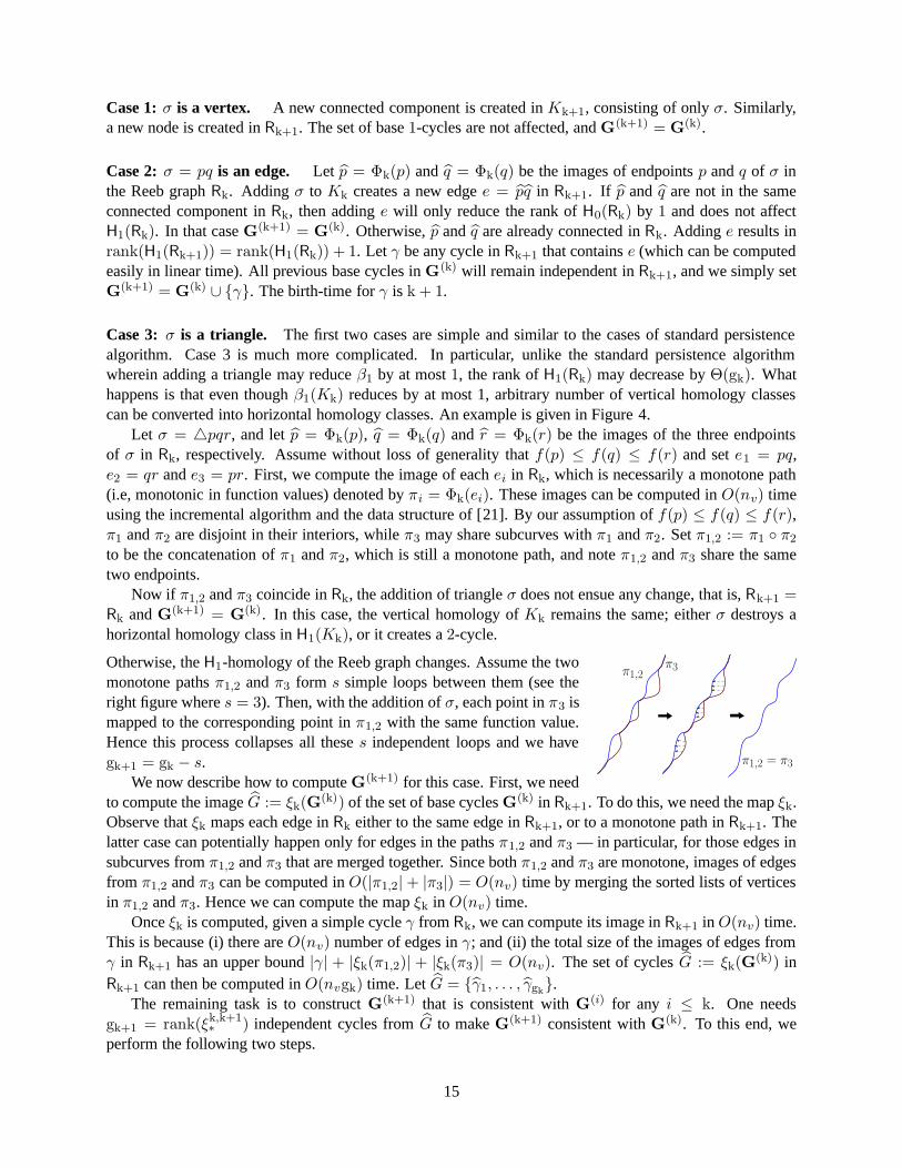
Otherwise, the H1-homology of the Reeb graph changes. Assume the twomonotone paths π1,2 and π3 form s simple loops between them (see theright figure where s = 3). Then, with the addition of σ, each point in π3 ismapped to the corresponding point in π1,2 with the same function value.Hence this process collapses all these s independent loops and we havegk+1 = gk − s.

We now describe how to compute G(k+1) for this case. First, we need

to compute the image G := ξk(G(k)) of the set of base cycles G

(k) in Rk+1. To do this, we need the map ξk.Observe that ξk maps each edge in Rk either to the same edge in Rk+1, or to a monotone path in Rk+1. Thelatter case can potentially happen only for edges in the paths π1,2 and π3 — in particular, for those edges insubcurves from π1,2 and π3 that are merged together. Since both π1,2 and π3 are monotone, images of edgesfrom π1,2 and π3 can be computed in O(|π1,2| + |π3|) = O(nv) time by merging the sorted lists of verticesin π1,2 and π3. Hence we can compute the map ξk in O(nv) time.

Once ξk is computed, given a simple cycle γ from Rk, we can compute its image in Rk+1 in O(nv) time.This is because (i) there are O(nv) number of edges in γ; and (ii) the total size of the images of edges fromγ in Rk+1 has an upper bound |γ| + |ξk(π1,2)| + |ξk(π3)| = O(nv). The set of cycles G := ξk(G

(k)) inRk+1 can then be computed in O(nvgk) time. Let G = {γ1, . . . , γgk

}.The remaining task is to construct G

(k+1) that is consistent with G(i) for any i ≤ k. One needs

gk+1 = rank(ξk,k+1∗ ) independent cycles from G to make G

(k+1) consistent with G(k). To this end, we

perform the following two steps.

15

(S1). We represent each cycle in G as a linear combination of cycles in a basis for the graph Rk+1.

(S2). We check the dependency of cycles in G in order of their birth-times, and remove redundant cycles toobtain G

(k+1).

Step (S1). Since Rk+1 is a graph, we compute a canonical basis of cycles, B = {α1, . . . , αgk+1}, in the

following standard way. Construct an arbitrary spanning tree T of Rk+1. Let E = {e1, . . . , egk+1} denote

the set of non-tree edges in Rk+1. Each edge ei = pq ∈ E creates a canonical cycle that concatenates edgeei with the two unique paths in T from p and q to their common ancestor. We set αi to be this canonicalcycle created by ei. Obviously, each ei appears exactly once among all cycles in B. Given a cycle γ ∈ G,we need to find coefficients cis such that γ =

∑gk+1

i=1 ciαi, where each ci is either 0 or 1. Since ei appearsonly in αi, we have ci equal the number of times ei appears in γ modulo 2. Since γ is a simple curve, ci is1 if ei ∈ γ and 0 otherwise. Hence all cis for i ∈ [1, gk+1] can be computed in O(nv) time for one curve γ.Computing the coefficients of all cycles in G takes O(nvgk) time.

Step (S2). Recall that cycles in G(k) = {γ1, . . . , γgk

} are sorted by increasing order of their birth-times.Note, the birth-time of the cycle γi ∈ G, which is the image of the cycle γi ∈ G

(k) in Rk+1, may be smallerthan the birth-time of γi. Now represent cycles in G with respect to the canonical basis B = {α1, . . . , αgk+1

}in a matrix M , where the ith column of M , denoted by colM [i], contains the coordinates of γi under basisB; that is, γi =

∑gk+1

j=1 colM [i][j]αj . Obviously, the matrix M has size gk × gk+1.Next, we perform a left-to-right reduction of matrix M , which is the same as the reduction of the

adjacency matrix used in the standard persistence algorithm [7, 16]. In particular, the only operation thatone can use is to add a column to another one on its right. For a column colM [i], let its low-row index denotethe largest index j such that colM [i][j] = 1. At the end of the reduction, each column is either empty orhas a unique low-row index; that is, no other column can have the same low-row index as this one. We setG

(k+1) as the subset of G whose corresponding columns in the reduced matrix M ′ is not all zeros. Thereduction takes time O(gk+1g

2k). Intuitively, the consistency of G

(k+1) with each G(i) for i ∈ [1, k] follows

from the left-to-right reduction. It guarantees that if a set of cycles in G are dependent, then only thosecreated earlier (i.e, with smaller birth-time) will be kept.

Lemma 5.2 G(k+1) as constructed above provides a basis of H1(Rk+1). Furthermore, if {G(1), . . . ,G(k)}

is consistent, so is {G(1), . . . ,G(k+1)}.

Proof: Let M ′ denote the reduced matrix of M . Recall that G = {γ1, . . . , γgk} contains the images of cycles

from G(k) in Rk+1. Set Gi = {γ1, . . . , γi} and let G′

i be the set of cycles from Gi whose correspondingcolumn in the reduced matrix M ′ is non-empty (i.e, not all zeros). In other words, G′

i = Gi ∩G(k+1) is the

intersection between Gi and the set G(k+1) constructed by our algorithm. By induction on i, it is easy to

show that for any i ∈ [1, gk], cycles in G′i generate the same subgroup of H1(Rk+1) as Gi. It then follows

that, in the end, cycles in G(k+1) = G′

gkare all independent in Rk+1 and |G(k+1)| equals the rank of the

homology group generated by cycles in G, which is βk,k+1 = gk+1. This proves the first part of the claim.For the second part of the claim, first note that G(k+1) is consistent with G

(k) as G∩G(k+1) = G

(k+1)

and has cardinality gk+1. Now consider an arbitrary G(i) with i < k. Since {G(1), . . . ,G(k)} are consistent,

and cycles {γ1, . . . , γgk} in G

(k) are sorted by their birth-times, it follows from Claim 5.1 that the firsts = βi,k number of cycles Gs = {γ1, . . . , γs} from G

(k) are images of cycles from G(i). Hence the

image of cycles from G(i) in Rk+1 are exactly the cycles in Gs, and classes of cycles in Gs generate the

persistent homology group ξi,k+1∗ (H1(Rf (Ki)). On the other hand, as mentioned above, classes of cycles in

G′s = Gs ∩ G

(k+1) generate the same subgroup of H1(Rk+1) as Gs. Since cycles in G′s are independent,

G′s has rank βi,k+1, implying that G

(k+1) is consistent with G(i), for any i ∈ [1, k]. The second part of the

claim then follows.

16

Finally, for our algorithm to continue into the next iteration, we also need to maintain the birth-times foreach cycle in G

(k+1). This is achieved by the following claim.

Claim 5.3 Let G(k+1) = {γI1 , . . . γIgk+1

}, where Iis are the set of indices of non-zero columns in thereduced matrix M ′. Then the birth-time of γIi

equals to the birth-time of γIifor any i ∈ [1, gk+1].

Proof: Recall that G(k+1) contains the set of cycles γIiwhere {Ii} is the set of indices of non-zero columns

from the reduced matrix M ′. Given a cycle α ∈ G(i), let birthtime(α) denote the birth-time of α. Assume

that one of the cycles, say γm ∈ G(k+1), has a birth-time that is different from that of γm ∈ G

(k). Sett := birthtime(γm). Since γm = ξk(γm), we have t ≤ birthtime(γm). Since the two birth-times aredifferent, t must be strictly smaller than the birth-time of γm.

Furthermore, there exists a cycle α ∈ Rt such that its image α1 := ξt,k(α) in Rk is not homologousto γm, while its image α2 := ξt,k+1(α) in Rk+1 is γm. On the other hand, α1 can be uniquely written asa linear combination of a subset of cycles from G

(k), say α1 = γJ1 + · · · + γJt . It is easy to verify thatthe birth-time of each γJi

is at most t. Since t < birthtime(γm), it follows that all indices Jis are strictlysmaller than m (as cycles in G

(k) are sorted by their birth-times). However, this is not possible since theresulting m-th column will be all zero at the time when we reduce the m-th column to construct G

(k+1) asγm =

∑i γJi

. Hence the cycle γm cannot be chosen as a base cycle in G(k+1) reaching a contradiction. It

follows that t = birthtime(γm), or more generally, birthtime(γIi) = birthtime(γIi

) for every index Ii

of non-zero column in the reduced matrix M ′.Putting everything together, we conclude with the following main result.

Theorem 5.4 Given a filtration K1 ⊂ · · · ⊂ Kn of a simplicial complex Kn with a piecewise linear functionf : Kn → IR, we can compute all persistent first betti numbers for the induced sequence of Reeb graphsRf (Ki)s in O(

∑ni=1(nvgi +g3

i )) = O(nn3e) time, where nv and ne are the number of vertices and edges in

Kn, respectively, n is the size of 2-skeleton of Kn, and gi is the first betti number of the Reeb graph Rf (Ki).

6 Conclusions and discussions

In this paper, we present a simple and efficient algorithm to approximate the Reeb graph Rf (M) of a mapf : M → IR from point data sampled from a smooth and compact manifold M. Given that Reeb graph isan abstract graph with a function defined on it, we only approximate its topology together with the rangeinformation for each loop in it. It will be interesting to see whether the Reeb graph we compute from thepoint data is also geometrically close to some specific embedding of the Reeb graph Rf (M) in the hiddendomain M. To this end, our results in Section 4.1 on mappings between cycles can be useful.

We also study how to compute the “persistence” of loops in a Reeb graph by measuring their life timeas the defining domain grows. An immediate question is to see whether the time complexity can be furtherimproved to match that of the standard persistence algorithm in the worst case.

Finally, it will be interesting to explore whether one can leverage the simple structure and efficient com-putation of the Reeb graph to retrieve topological information for various spaces efficiently. For example,given a 3-manifold with a function f defined on it, its vertical H1-homology is already encoded in the Reebgraph and can thus be computed in near-linear time. Can we retrieve the horizontal H1-homology efficientlyby tracking the levelsets of f , or by defining another function that is somewhat “orthogonal” to f?

17

Acknowledgments.

The authors thank anonymous reviewers for helpful comments. This work is supported by National ScienceFoundation under grants CCF-0915996, CCF-1116258 and CCF-1048983.

References

[1] M. Bernstein, V. de Silva, J. Lanford, and J. Tenenbaum. Graph pproximations to geodesics on em-bedded manifolds. Technical report, Dept. Psychology, Stanford University, USA, 2000.

[2] S. Biasotti, D. Giorgi, M. Spagnuolo, and B. Falcidieno. Reeb graphs for shape analysis and applica-tions. Theor. Comput. Sci., 392(1-3):5–22, 2008.

[3] F. Chazal, L. J. Guibas, S. Oudot, and P. Skraba. Analysis of scalar fields over point cloud data. InProc. 20th ACM-SIAM Sympos. Discrete Algorithms, pages 1021–1030, 2009.

[4] F. Chazal, L. J. Guibas, S. Y. Oudot, and P. Skraba. Persistence-based clustering in Riemannian mani-folds. In Proc. 27th Annu. Sympos. Comput. Geom., pages 97–106, 2011.

[5] F. Chazal and S. Oudot. Towards persistence-based reconstruction in Euclidean spaces. In Proc. 24thACM Sympos. on Comput. Geom., pages 232–241, 2008.

[6] D. Cohen-Steiner, H. Edelsbrunner, and J. Harer. Extending persistence using Poincare and Lefschetzduality. Foundations of Computational Mathematics, 9(1):79–103, 2009.

[7] D. Cohen-Steiner, H. Edelsbrunner, and D. Morozov. Vines and vineyards by updating persistence inlinear time. In Proc. 22nd Annu. Sympos. Comput. Geom., pages 119–126, 2006.

[8] K. Cole-McLaughlin, H. Edelsbrunner, J. Harer, V. Natarajan, and V. Pascucci. Loops in Reeb graphsof 2-manifolds. Discrete Comput. Geom., 32(2):231–244, 2004.

[9] T. K. Dey. Curve and Surface Reconstruction: Algorithms with Mathematical Analysis. Cambridge U.Press, New York, NY, USA, 2007.

[10] T. K. Dey and K. Li. Cut locus and topology from surface point data. In Proc. 25th Annu. Sympos.Comput. Geom., pages 125–134, 2009.

[11] T. K. Dey, J. Sun, and Y. Wang. Approximating loops in a shortest homology basis from point data. InProc. 26th Annu. Sympos. Compu. Geom., pages 166–175, 2010.

[12] H. Doraiswamy and V. Natarajan. Efficient output-sensitive construction of Reeb graphs. In Proc. 19thInternat. Sym. Alg. and Comput., pages 556–567, 2008.

[13] H. Doraiswamy and V. Natarajan. Efficient algorithms for computing Reeb graphs. ComputationalGeometry: Theory and Applications, 42:606–616, 2009.

[14] H. Edelsbrunner and J. Harer. Persistent homology — a survey. In J. E. Goodman, J. Pach, andR. Pollack, editors, Surveys on Discrete and Computational Geometry. Twenty Years Later, pages257–282. Amer. Math. Soc., Providence, Rhode Island, 2008. Contemporary Mathematics 453.

[15] H. Edelsbrunner, J. Harer, A. Mascarenhas, V. Pascucci, and J. Snoeyink. Time-varying Reeb graphsfor continuous space-time data. Comput. Geom., 41(3):149–166, 2008.

18

[16] H. Edelsbrunner, D. Letscher, and A. Zomorodian. Topological persistence and simplification. DiscreteComput. Geom., 28:511–533, 2002.

[17] W. Harvey, R. Wenger, and Y. Wang. A randomized O(m log m) time algorithm for computing Reebgraph of arbitrary simplicial complexes. In Proc. 26th Annu. Sympos. Compu. Geom., pages 267–276,2010.

[18] J.-C. Hausmann. On the Vietoris-Rips complexes and a cohomology theory for metric spaces. InProspects in Topology: Proc. Conf. in Honour of William Browder, Ann. Math. Stud., 138, pages175–188. Princeton Univ. Press, 1995.

[19] J. R. Munkres. Elements of Algebraic Topology. Westview Press, 1996.

[20] P. Niyogi, S. Smale, and S. Weinberger. Finding the homology of submanifolds with high confidencefrom random samples. Discrete Comput. Geom., 39:419–441, 2008.

[21] V. Pascucci, G. Scorzelli, P.-T. Bremer, and A. Mascarenhas. Robust on-line computation of Reebgraphs: simplicity and speed. ACM Trans. Graph., 26(3):58, 2007.

[22] Y. Shinagawa and T. L. Kunii. Constructing a Reeb graph automatically from cross sections. IEEEComput. Graph. Appl., 11(6):44–51, 1991.

[23] J. Tierny, A. Gyulassy, E. Simon, and V. Pascucci. Loop surgery for volumetric meshes: Reeb graphsreduced to contour trees. IEEE Trans. Vis. Comput. Graph., 15(6):1177–1184, 2009.

A Proof for Lemma 4.2

The second part of claim (ii) follows immediately from Claim 4.1.The first part of claim (ii) follows fromclaim (i). Hence we focus on proving claim (i). First, we show the following two claims: (C-1) given a cycleα from Z1(M), [α] = [h#(d(α))]; and (C-2) given a cycle α ∈ Z1(R

r(P )), we have that [α] = [d(h#(α))].Note that cycles in Z1(R

r(P )) are simplicial cycles, while cycles in Z1(M) are singular cycles.

Proving (C-1). We show that given a cycle α from Z1(M), [α] = [h#(d(α))]. Let γ ⊆ M be the carrierof α. To map α to d(α), suppose that its carrier γ is broken into k pieces as described earlier using theDecomposition method. For the i-th piece with endpoints xi and xi+1, let pi and pi+1 be their closest pointin P , respectively; recall that d(α) is the concatenation of all edges pipi+1 for i ∈ [1, k].

Now consider the cycle h#(d(α)) in M: its carrier γ ′ is the concatenation of h(pipi+1) ⊂ M for alli ∈ [1, k]. By Proposition 3.3 of [11], each curve h(pipi+1) has endpoints pi and pi+1, and it is containedin the union of the two Euclidean balls of radius r centered at pi and at pi+1. Since pi and pi+1 are withinr Euclidean distance, h(pipi+1) is contained in the Euclidean balls of radius 2r centered at pi and at pi+1.Notice that the geodesic distance and the Euclidean distance between two points x, y ∈ M approximateeach other when x and y are close enough (see e.g, Proposition 1.2 from [11]). It follows that when r issmaller than ρ(M)/4, h(pipi+1) is contained in both geodesic balls of radius 3r centered at pi ∈ M andpi+1 ∈ M.

Let γ[xi, xi+1] denote the subcurve of γ from xi to xi+1. Since the length of γ[xi, xi+1] is less than rby construction, the curve γ[xi, xi+1] is contained in the geodesic balls of radius r centered at xi and xi+1.This implies that the curve γ[xi, xi+1] is contained in the geodesic tubular neighborhood

Tubr(πg(xi, xi+1)) := {y ∈ M | d(y, πg(xi, xi+1)) ≤ r}

19

where πg(x, y) denote a minimizing geodesic between two points x, y ∈ M. By Proposition 3.7 of [11],Tubr(πg(xi, xi+1)) is contractible and hence γ[xi, xi+1] is homotopy equivalent to πg(xi, xi+1).

On the other hand, due to the sampling condition, the geodesic distances between xi and pi, and be-tween xi+1 and pi+1, are both bounded by r. Combining this with the fact that h(pipi+1) lies within thegeodesic balls of radius 3r centered at both pi and pi+1, we have that any point in h(pipi+1) is withingeodesic distance 4r to both xi and to xi+1. Hence h(pipi+1) lies within the geodesic tubular neighbor-hood Tub4r(πg(xi, xi+1)). Again by Proposition 3.7 of [11], when r ≤ ρc(M)/4, the curve πg(xi, pi) ◦h(pipi+1)◦πg(pi+1, xi+1) is homotopy equivalent to πg(xi, xi+1) and thus homotopy equivalent to γ[xi, xi+1].In fact, one can find a homotopy hi that keeps pi and pi+1 on the geodesics πg(xi, pi) and πg(xi+1, pi+1)respectively so that two maps hi and hi+1, for i ∈ [1, k − 1], are consistent in mapping the common end-points xi+1. Therefore, we can combine all such hi’s to obtain a homotopy between γ ′ (which is the carrierof h#(d(α))) and γ (which is the carrier of α). It follows that [h# ◦ d(α)] = [α].

Proving (C-2). We now show that given any (simplicial) cycle α ∈ Z1(Rr(P )), we have that [α] =

[d ◦h#(α)]. First, consider the image γ = h(α) of α in M; γ is the carrier of the cycle h#(α) ∈ Z1(M). Byconstruction, γ is the concatenation of h(e)s for every edge e = pq in the simplicial cycle α. By Proposition3.3 in [11], each curve h(e) is contained inside M ∩ (Br(p) ∪ Br(q)). Hence, for any point x ∈ h(e), itsgeodesic distance to p and to q is bounded by 3r.

Now consider mapping the cycle h#(α) carried by γ back to Rr(P ) using the decomposition methoddescribed earlier. Consider the set of breaking points xi’s in the subcurve h(e) ⊂ γ — assume for simplicitythat the endpoints of h(e), that is p and q, are also break points. Each break point xi in h(e) will be mappedto its nearest point pi ∈ P and the geodesic distance between xi and pi is at most r. Hence pi is within3r + r = 4r geodesic distance to both endpoints p and q of the edge e ⊂ α. This means that both pip andpiq are edges in the Rips complex R4r(P ). Hence the concatenation of arcs pipi+1 is homotopy equivalentto the edge e in the simplicial complex R4r(P ). Combining this homotopy equivalent map for every edgee ∈ α, we have that d(h#(α)) is homotopy equivalent, and thus homologous, to α in R4r(P ). Finally, sincethe inclusion map from Rr(P ) to R4r(P ) induces an isomorphism in the first homology groups when r issmall, we have that d(h#(α)) is homologous to α in Rr(P ) as well. Thus [α] = [d(h#(α))].

Proving Claim (i). (C-1) and (C-2) imply that d is the homology-inverse of the map h#. The map h#

induces an isomorphism h∗ : H1(Rr(P )) → H1(M). Hence d also induces an isomorphism in the homology

groups H1(M) → H1(Rr(P )).

Proving Claim (iii). Claim (iii) follows easily from the constructions of d and h. In particular, consider acycle α ∈ Z1(M) and d(α) ∈ Z1(R

r(P )). (The case for α from Z1(Rr(P )) and h#(α) from Z1(M) can

be similarly argued.) Let γ ⊂ M be the carrier of α. The Decomposition method breaks γ into k piecesγ(xi, xi+1)s, for i ∈ [0, k]. Each piece γ(xi, xi+1) is mapped to the edge pipi+1 where pi is the closestpoint of xi in P . Since P is an ε-sample of M, and since the length of γ(xi, xi+1) is at most r − 2ε, anypoint x in γ(xi, xi+1) is within r geodesic distance to the point pi ∈ M. Hence by the Lipschitz conditionof f , we have |f(xi) − f(pi)| ≤ r · Lipf . It follows that

[ mini∈[0,k]

f(pi) + r · Lipf , maxi∈[0,k]

f(pi) − r · Lipf ] ⊆ range(γ) = range(α)

⊆ [ mini∈[0,k]

f(pi) − r · Lipf , maxi∈[0,k]

f(pi) + r · Lipf ].

On the other hand, note that under Z2 coefficient, range(d(α)) ⊆ [mini∈[0,k] f(pi),maxi∈[0,k] f(pi)] (andit can be much smaller than this interval). It then follows that range(d(α)) is oneside-(r · Lipf )-close torange(α).

20

Proof of Claim (iv). Consider any homology class ω ∈ H1(M). By Claim (iii) we have that the rangeof d∗(ω) is oneside-(r · Lipf )-close to the range of ω: indeed, choose the thinnest cycle α of ω, we haverange(d(α)) is oneside-(r · Lipf )-close to range(α) = range(ω). Since range(d∗(α)) ⊆ range(d(γ)),range(d∗(α)) is also oneside-(r · Lipf )-close to range(ω).

Now map d∗(ω) back to H1(M), we have that the range of h∗(d∗(ω)) is also oneside-(r · Lipf )-close tothe range of d∗(ω) by Claim (iii). Since h∗(d∗(ω)) = ω, the ranges of ω and d∗(ω) are (r ·Lipf )-Hausdorff-close.

The statement for ω and h∗(ω) can be argued similarly.

21