Abstract In this paper, we present a novel algorithm thatcombines the power of expression of Geometric Algebrawith the robustness of Tensor Voting to find the correspon-dences between two sets of 2D points with an underlyingrigid transformation. Unlike other popular algorithms forpoint registration (like the Iterated Closest Points), our algo-rithm does not require an initialization, works equally wellwith small and large transformations between the data sets,performs even in the presence of large amounts of outliers(90% and more), and have less chance to be trapped in “lo-cal minima”. Furthermore, we will show how this algorithmcan be easily extended to account for multiple overlappingmotions and certain non-rigid transformations.
In this paper we address the problem of finding the corre-spondences of two point sets in 2D assuming that a rigidtransformation has taken place without further information.These correspondences enable us to compute the motion be-tween these sets to perform registration. The problem of reg-istering data sets is common in the computer vision litera-ture. Applications range from the alignment of range mea-
L. Reyes-Lozano · E. Bayro-Carrochano (�)Department of Electrical Engineering and Computer Science,CINVESTAV, Unidad Guadalajara, Jalisco, Mexicoe-mail: [email protected]
G. MedioniInstitute for Robotics and Intelligence Systems, Universityof Southern California, Los Angeles, CA, USA
surements for the automatic re-construction of maps for ro-botic navigation [14, 19]; registration of CT and MR imagesfor medical purposes [8, 10, 11, 18, 24]; computer graph-ics and CAD modeling [7, 26] and recognition of objects[3, 27].
2 State of the Art
The classical solution to this problem was given by Besl andMcKay with the Iterative Closest Points algorithm (ICP) [2].Several improvements have been made to the basic schemestarting with a more efficient way to compute the distanceand thresholding of the points [29] by the use of K-D treesand statistical analysis, respectively; the use of extra cuesto improve the matching of points like texture [12, 15]; theimplementation of a soft-assign scheme to allow for varyingdegrees of certainty in the matches [27]; and the use of morerobust iteration techniques like Levenberg-Marquardt [4, 9].
The advantages of the ICP are that it is simple, fast,and hence can be used for real-time applications. However,in general, all the ICP-based approaches refine an initialguess of the registration by iteratively updating the parame-ters of the transformation. If the initialization is poor, themethod will not converge to the desired solution. Becauseof this, ICP is generally used when the difference betweenthe model and the data is small, constraining the range ofpossible applications to those where this constraint can bemet. One way to overcome this problem is by initializingthe transformation with other methods like the Procrustes[20] algorithm. Another drawback of this method is that itrequires a model and a data set, so that the data set is asubset of the model. That is, at least one of the data setsmust not contain outliers (the model) and must be relativelynoise-free. Also, the ICP in general is not robust against the
presence of outliers, and is limited to registering points viaa rigid transformation. Another disadvantage is that the re-sulting mapping may not be one-to-one.
Another method widely used to solve the registrationproblem is Chamfer matching [3]. In this paper, Borgeforsimproves the original chamfer matching algorithm by usinga resolution pyramid in a hierarchical matching procedure.Chamfer matching can also be implemented in a parallelfashion [28] to improve its performance. Again, the limi-tation of this method is that the motion between the imagesmust be small or the process might converge to a local min-imum. The images must also be free of outliers.
Methods that do not require initialization and are ro-bust to outliers are generally based on voting schemes, likethe Hough Transform. Kalviainen et al use the RandomizedHough Transform [16], for example, to obtain the 2D mo-tion between two point sets. The advantages of this methodis that it does not require an initialization and works equallywell independently of the “size” of the transformation. How-ever, due to the inherent discretization of the transforma-tion space, the range of possible motions becomes limitedin range and precision. This becomes an issue when largeamounts of outliers are present. We will show in this paperhow Tensor Voting does not suffer from this problem. Fi-nally, another disadvantage of this method is that it is basedon a model that must be free of outliers and relatively lownoise level.
Finally, in the voting-based algorithms. Kang et al. [17]demonstrated how Tensor Voting can be used to detect mul-tiple affine motions in 2D. It should be noted that all thealgorithms mentioned so far only work when a single globalmotion is present in the data. Kang’s algorithm is largely in-dependent of initialization (it allows for multiple candidatematches and has a robust way of rejecting the false matches),and is robust to outliers. This paper is inspired by the workof Kang, therefore, we will discuss the similarities and dif-ferences of both algorithms in a subsequent section.
There are also a few algorithms that handle non-rigidtransformations like [5] which uses soft-assign and an iter-ative minimization method (deterministic annealing) to pro-duce a non-rigid registration of points. The advantage of thismethod is that it guarantees a one-to-one mapping when thealgorithm finishes, but the disadvantage is that it requires agood initialization and only withstands a small amount ofoutliers in the input data. Another ICP-based algorithm thatperforms non-rigid (affine and spline) registration is givenin [8], the same disadvantages of initialization and outliersapply. Finally, in [18] B-splines are used to perform the reg-istration and gradient descent technique is used to find thesolution. This approach is dependent on a good initializa-tion. Generally, these methods find a greater application formedical imaging.
Another type of problem is the registration of multipledata sets. Solutions to this problem have been reviewed
in [6]. One solution consists mainly of expressing the prob-lem as an optimization problem where the parameters areall the transformations needed to register the multiple datasets [10] and then a standard minimization algorithm is used.Another approach relies on modeling the problem as a dy-namic spring system to register the multiple sets together[7, 25]. These algorithms suffer from the same problemsthat have been already mentioned: they require an initializa-tion and, depending on its quality, may or may not convergeto the desired solution, and they are not robust against thepresence of outliers. However, we will restrict ourselves tothe two-frame case only. Finally, using other mathematicalframeworks there are applications in medical imaging regis-tration which use a Lie group approach [22] and conformalgeometric algebra [1].
In general, the ICP and Chamfer matching based algo-rithms suffer from the following disadvantages.
• A good initialization must be provided. The quality of theinitial correspondences impacts the performance of the al-gorithms.
• The range of possible motions is restricted (they work bet-ter for small motions).
• No outliers are permitted in the model and few to none inthe data.
• Require preprocessing of the data to reject outliers (ifpresent).
• Only work when a single global rigid motion is present.• For the gradient-descent and Levenberg-Marquardt im-
plementations, a computation of the derivatives is needed.• The resulting mapping is not guaranteed to be one-to-one.
For the Hough-based algorithms, the disadvantages are
• The range of the possible transformations is limited dueto the size of the voting space.
• The voting space introduces a quantization of the parame-ters which compromises the accuracy of the solution.
In this paper we propose a novel algorithm that providesthe following advantages.
• Robust to large numbers of outliers.• No initialization required.• No thresholding to reject incorrect pairings needed (as is
the case for most ICP implementations).• Works equally well for large and small motions.• No quantization is introduced for the parameters of the
transformation, the accuracy of the solution is thereforenot compromised.
• Does not require any preprocessing of the data.• Does not require estimation of derivatives.• Guarantees a one-to-one correspondence.• Multiple overlapping motions can be detected.
J Math Imaging Vis (2010) 37: 249–266 251
2.1 Affine 2D Motion Estimation Using Tensor Voting
As mentioned in previous paragraphs, this work was largelyinspired by Kang’s paper [17]. We would like to discuss herapproach in some detail here.
Kang begins with the six-parameter 2D affine transfor-mation equation
[x′y′
]=
[a b
c d
][x
y
]+
[txty
], (1)
which transforms a 2D point (x, y) into (x′, y′). This equa-tion can be rewritten as[a b −1 0 txc d 0 −1 ty
][x y x′ y′ 1
]T = 0. (2)
From this equation it can be clearly seen that we actuallyhave the following separate joint spaces
[a b −1 tx
] [x y x′ 1
]T = 0, (3)
and
[c d −1 ty
] [x y y′ 1
]T = 0, (4)
which correspond to two independent 3D spaces in the ho-mogeneous coordinates (x, y, x′,1) and (x, y, y′,1). It isalso easy to see that any correspondence pair (x, y) ↔(x′, y′) obeying such an affine transformation will producetwo points in these joint spaces which lie on the 3D planes(a, b,−1, tx) and (c, d,−1, ty).
From this observation, Kang proceeds to populate bothjoint spaces with a set of tentative correspondences. Thesecorrespondences might contain a large amount of outliers(wrong correspondences). The outliers were dealt with byapplying Tensor Voting to find the actual planes which rep-resented the affine motion.
2.2 Our Approach
Based on these results, we tried to answer the followingquestion: By restricting the problem to rigid motion, wasis possible to produce a further simplification of the prob-lem? It was clear that Kang’s approach could also detectrigid motion since it is just a special case of the affine mo-tion. However, by restricting the problem to detecting rigidmotion only, a simplification of the detection process shouldalso be possible.
We followed Kang’s procedure and began by writingdown the equation of rigid motion in 2D
[x′y′
]=
[cos(θ) − sin(θ)
sin(θ) cos(θ)
][x
y
]+
[txty
]. (5)
This equation can be rewritten as
[cos(θ) − sin(θ) −1 0 txsin(θ) cos(θ) 0 −1 ty
]
× [x y x′ y′ 1
]T = 0. (6)
But we end up with the same joint space which consists oftwo 3D spaces. It was clear that no further simplification waspossible unless we used a different parameterization whichdisentangled the inner dependency between the sine and co-sine inside the transformation matrix. Therefore, we turnedour attention to Geometric Algebra to accomplish this task.
Even though we will save the details about Geometric Al-gebra and the formulation of our problem for the followingsections, we will present a summary here. In Geometric Al-gebra of the 2D space, the rigid transformation of a pointcan be written as
x′ = RxR + t, (7)
where R = eθ2 σ12 = cos( θ
2 ) + sin( θ2 )σ12 represents the ro-
tation and t = txσ1 + tyσ2 is a translation vector. From theprevious equation, by left-multiplication with R we get
Rx′ = xR + Rt, (8)(cos
(θ
2
)+ sin
(θ
2
)σ12
)(x′σ1 + y′σ2)
= (xσ1 + yσ2)
(cos
(θ
2
)+ sin
(θ
2
)σ12
)
+(
cos
(θ
2
)+ sin
(θ
2
)σ12
)(txσ1 + tyσ2). (9)
Developing products and factoring the results we get the fol-lowing equations
[− sin(
θ2
)cos
(θ2
)(sin
(θ2
)tx − cos
(θ2
)ty)
]× [
(x′ + x) (y′ − y) 1]T = 0, (10)[
sin(
θ2
)cos
(θ2
) −(cos(
θ2
)tx + sin
(θ2
)ty)
]× [
(y′ + y) (x′ − x) 1]T = 0. (11)
Which are clearly the equations of two lines in the jointspaces (x′+x), (y′ −y) and (y′+y), (x′−x). Hence, by ap-plying Geometric Algebra we simplified the problem fromfinding two independent 3D planes to detecting two non-independent 2D lines. This dependency between the spacesworks to our advantage too: it will be shown in subsequentsections that there is a geometric constraint between bothlines which further confirms a correct rigid transformationhas been detected and also helps in rejecting false or multi-ple matches.
252 J Math Imaging Vis (2010) 37: 249–266
We believe that this simplification is not possible usingthe traditional matrix representation of the rigid transforma-tion, since the key step was a left-multiplication by the in-verse of the rotor. This was necessary because the transfor-mation equation requires a left and right multiplication inorder to rotate a 2D point in Geometric Algebra. Recentlythis approach was extended for registration of 3D points,see [23].
2.3 Structure of the Paper
The structure of the paper is as follows. Section 3 gives abrief description of the Tensor Voting methodology for thedetection of curves in 2D. Section 4 introduces GeometricAlgebra. In Sect. 5 we describe how we used the Geomet-ric Algebra to re-cast the problem as a problem of detect-ing 2 lines in 2D. Next, we describe the core of our algo-rithm in Sect. 6, followed by a series of tests with syntheticdata to validate it in Sect. 7 and a more formal analysis inSect. 8. Experimental results with real data are presented inSect. 9, along with the extensions needed for multiple mo-tions and non-rigid motion estimation. The Conclusions fol-low in Sect. 10.
3 Tensor Voting
Tensor voting is a methodology for the extraction of denseor sparse features from nD data. Some of the features thatcan be detected with this meth odology include lines, curves,points of junction and surfaces.
The Tensor Voting methodology is grounded in two el-ements: tensor calculus for data representation and tensorvoting for data communication. Each input site propagatesits information in a neighborhood (the information itselfis encoded as a tensor and is defined by a predefined vot-ing field). Each site collects the information cast there byits neighbors and analyzes it, building a saliency map foreach feature type. Salient features are located at local ex-trema of these saliency maps, which can be extracted bynon-maximal suppression.
For the present work, we found that sparse tensor vot-ing, along with Geometric Algebra, was enough to solvethe problem. Also, we only needed the detection of lines (orcurves) in 2D. Therefore we will confine our explanation oftensor voting to this particular process. The interested readermay find further information in [21].
3.1 Tensor Representation in 2D
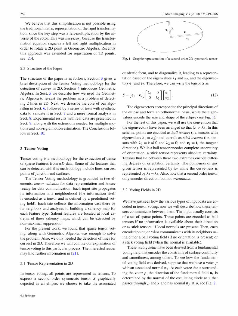
In tensor voting, all points are represented as tensors. Toexpress a second order symmetric tensor S graphicallydepicted as an ellipse, we choose to take the associated
Fig. 1 Graphic representation of a second order 2D symmetric tensor
quadratic form, and to diagonalize it, leading to a represen-tation based on the eigenvalues λ1 and λ2, and the eigenvec-tors e1 and e2. Therefore, we can write the tensor S as
S = [e1 e2
][λ1 00 λ2
][e1
e2
]. (12)
The eigenvectors correspond to the principal directions ofthe ellipse and form an orthonormal basis, while the eigen-values encode the size and shape of the ellipse (see Fig. 1).
For the rest of this paper, we will use the convention thatthe eigenvectors have been arranged so that λ1 > λ2. In thisscheme, points are encoded as ball tensors (i.e. tensors witheigenvalues λ1 = λ2), and curvels as stick tensors (i.e. ten-sors with λ1 = k �= 0 and λ2 = 0; and e1 = t, the tangentdirection). While a ball tensor encodes complete uncertaintyof orientation, a stick tensor represents absolute certainty.Tensors that lie between these two extremes encode differ-ing degrees of orientation certainty. The point-ness of anygiven tensor is represented by λ2 while the curve-ness isrepresented by λ1 −λ2. Also, note that a second order tensoronly encodes direction, but not orientation.
3.2 Voting Fields in 2D
We have just seen how the various types of input data are en-coded in tensor voting, now we will describe how these ten-sors communicate between them. The input usually consistsof a set of sparse points. These points are encoded as balltensors if no information is available about their directionor as stick tensors, if local normals are present. Then, eachencoded point, or token communicates with its neighbors us-ing either a ball voting field (if no orientation is present) ora stick voting field (when the normal is available).
These voting fields have been derived from a fundamentalvoting field that encodes the constrains of surface continuityand smoothness, among others. To see how the fundamen-tal voting field was derived, suppose that we have a voter p
with an associated normal np . At each votee site x surround-ing the voter p, the direction of the fundamental field nx isdetermined by the normal of the osculating circle at x thatpasses through p and x and has normal np at p, see Fig. 2.
J Math Imaging Vis (2010) 37: 249–266 253
The strength of the fundamental field s(d, ρ, σ ) at eachpoint depends on the distance d and curvature ρ between p
and x and is given by the following Gaussian function
s(d, ρ, σ ) = e−(
|d2|+ρ2
σ2 ), (13)
where σ is a scale factor that determines the overall rate ofattenuation. The shape of the fundamental field can be seenin Fig. 3.
Finally, both orientation and strength are encoded as astick vote. Hence, each voting site is also encoded as a ten-sor, and communication is performed by the addition of thetensor present at the votee and the tensor produced by thefield at that site.
The fundamental voting field, in the 2D case, is also thestick voting field. The stick voting field can be used whenthere is information about the local normal of the token.However, when no information is available, we must use theball voting field. This field is produced by rotating the fun-damental field and integrating the contributions at each sitesurrounding the voter. The resulting field is shown in Fig. 4.
Fig. 2 The osculating circleand the corresponding normalsof the voter and votee
3.3 Sparse Tensor Voting in 2D
Now that we have defined the tensors used to encode theinformation and the voting fields, we can describe the sparsevoting process.
If no information is available about the normals at eachtoken, we initialize them all as ball tensors. Then, in order toacquire the preferred orientations at each token, we place aball voting field at each voter and cast votes to all the neigh-bors. The process is repeated until all tokens have cast votesto all their neighbors. Once this step is finished, we can ex-tract the preferred orientations of each token by analyzingthe eigensystem encoded in its tensor. The preferred direc-tion is given by the eigenvector e1, and the saliency of thisorientation is given by λ1 − λ2.
To enforce the orientation of the tokens, or if we have thenormals available from the beginning, a sparse stick votingis performed. In this case, a stick voting field is placed oneach token and is rotated until it becomes aligned with thelocal normal. Then, the resulting field is used to cast votesto all the neighbors and reinforce the local normals.
After the voting stage is finished. The tensors at each siteare decomposed into their eigensystem. The resulting eigen-value λ1 encodes the absolute saliency of the token. Thisvalue roughly represents the number of neighbors that havelent support to this token. Tokens that are isolated will havea low absolute value and can be discarded as noise. Fromthe remaining tokens, we can identify which ones belong toa curve or a junction as follows. If λ1 � λ2, then there isa high confidence about the orientation of the token, and itbelongs to a curve. On the contrary, if λ1 ≈ λ2, then there isno preferred orientation and the token belongs to a junction.
Fig. 3 The fundamental voting field. Orientation and strength fields (left and center, respectively). 3D display of the strength field (right)
Fig. 4 The ball voting field.Orientation and strength fields(left and center, respectively).3D display of the strength field(right)
254 J Math Imaging Vis (2010) 37: 249–266
In this work, we have also used another curve-ness mea-sure that is independent of the absolute saliency of the to-ken. We simply take the ratio λ2/λ1. If the token belongs toa curve, the ratio will be close to 0. On the other hand, ifthe token is not oriented, the ratio becomes closer to 1. Thisis useful to find tokens with a low saliency but with a highorientation.
In the general formalism, after the preferred directionshave been obtained, a dense tensor voting is performed. Inthis stage, each voting field casts votes all around the spacesurrounding the voter (not only to neighboring tokens), andfeatures are extracted by performing an analysis that de-tects maxima from the dense junction and curvature saliencymaps. However, since we did not need that part of the enginein our present work, we refer the interested reader to [21] formore details.
4 Geometric Algebra
The main alternative to the classical approach to computervision is Clifford Geometric Algebra. This algebra sys-tem was invented by the English mathematician WilliamKingdom Clifford (1845–1879) who combined the ideas in-troduced by the German mathematician Hermann GüntherGrassmann (1809–1877) and Sir William Rowan Hamilton(1805–1865). Since the 1960s, David Hestenes has beenworking on developing his version of Clifford Algebra [13].We will now present a brief introduction to Geometric Al-gebra.
Geometric Algebra is enabled with a new product (theClifford product) that has an inverse (in general) and com-bines the properties of the inner and exterior products. Thatis to say, for two vectors a and b, their Clifford product isexpressed as
ab = a · b + a ∧ b, (14)
where · stands for the inner product and the wedge product∧ is similar to the cross product; but instead of producing avector, a new entity, called a bivector is rendered. The bivec-tor a ∧ b can be visualized as the oriented plane spanned bya and b. The Clifford product is linear, associative and anti-commutative, that is
ab = −ba (15)
and
a ∧ b = −b ∧ a. (16)
From (14), we can see that the Clifford product of a vec-tor with itself produces a scalar. In general, this scalar willnot be necessarily positive. By definition, in a geometric al-gebra Gp,q,r , the first p basis vectors σ1, . . . , σp will square
to 1, the next q basis vectors ep+1, . . . , ep+q will square in−1 and the last r basis vectors will square to 0.
Inside this mathematical framework, the common geo-metric algebra of 2D space G2,0,0 is spanned by
⎧⎨⎩ 1︸︷︷︸
scalar
, e1, e2︸ ︷︷ ︸vectors
, e21 ≡ I︸ ︷︷ ︸bivector
⎫⎬⎭ . (17)
The elements that span a given geometric algebra are calledblades. The grade of a blade indicates the number of basisvectors used to form it. That is to say, a scalar is a zero-gradeblade and the element e12 is a three-grade blade; however,in general, blades will be multiplied by a scalar factor. Theblade with the greatest grade in any given algebra is calledthe pseudoscalar and is commonly represented by the let-ter I . A k-vector is a linear combination of blades of grade k.A multivector is a linear combination of k-vectors of differ-ent grades. For any given multivector A, the notation 〈A〉rindicates the component r-vector of A (if the subindex isomitted, the scalar part is assumed). The grade of a multi-vector is the highest grade of its component blades. Usingthe grade notation, we can express the Clifford product ofany two given multivectors Ar and Bs of grade r and s, re-spectively, as
From this equation, we can derive the general definition forthe interior and exterior product for multivectors as
Ar · Bs = 〈ArBs〉|r−s|, (19)
Ar ∧ Bs = 〈ArBs〉r+s . (20)
Finally, for an r-grade multivector Ar = ∑ri=0〈Ar〉i , the
following operations are defined
Grade Involution: Ar =r∑
i=0
(−1)i〈Ar〉i , (21)
Reversion: Ar =r∑
i=0
(−1)i(i−1)
2 〈Ar〉i , (22)
Clifford Conjugation: Ar = ˜Ar =r∑
i=0
(−1)i(i+1)
2 〈Ar 〉i .(23)
The grade involution simply negates the odd-grade bladesof a multivector. The reversion can also be obtained by re-versing the order of basis vectors making up the blades in amultivector and then rearranging them to their original or-der using the anticommutativity of the Clifford product. The
J Math Imaging Vis (2010) 37: 249–266 255
Clifford conjugation can be used to compute the inverse ofa vector a as
a−1 = aaa
. (24)
This formula for the inverse can also be applied for k-vectorsbut cannot be used for all multivectors in general.
4.1 The Geometric Algebra of 3-D Space
The basis for the geometric algebra G3,0,0 of the 3-D spacehas 23 = 8 elements and is given by:
1︸︷︷︸scalar
, e1, e2, e3︸ ︷︷ ︸vectors
, e1e2, e2e3, e3e1︸ ︷︷ ︸bivectors
, e1e2e3 ≡ I︸ ︷︷ ︸trivector
.
In G3,0,0 a typical multivector v will be of the form v = α0 +α1e1 + α2e2 + α3e3 + α4e2e3 + α5e3e1 + α6e1e2 + α7I3 =〈v〉0 + 〈v〉1 + 〈v〉2 + 〈v〉3, where the αi ’s are real num-
bers and 〈v〉0 = α0 ∈0∧
V n, 〈v〉1 = α1e1 + α2e2 + α3e3 ∈1∧
V n, 〈v〉2 = α4e2e3 + α5e3e1 + α6e1e2 ∈2∧
V n, 〈v〉3 =α7I3 ∈
3∧V n.
In geometric algebra a rotor (short name for rotator),R, is an even-grade element of the algebra which satisfiesRR = 1, where R stands for the conjugate of R using (23).
If A = {a0, a1, a2, a3} ∈ G3,0,0 represents a unit quater-nion, then the rotor which performs the same rotation is sim-ply given by
R = a0︸︷︷︸scalar
+a1(Ie1) − a2(Ie2) + a3(Ie3)︸ ︷︷ ︸bivectors
= a0 + a1e2e3 − a2e3e1 + a3e1e2. (25)
The quaternion algebra is therefore seen to be a subset ofthe geometric algebra of 3-space. According to (23) for the3D Euclidean geometric algebra the conjugate of the rotor isR = a0 − a1e2e3 + a2e3e1 − a3e1e2.
The transformation in terms of a rotor a �→ RaR = b isa very general way of handling rotations; it works for multi-vectors of any grade and in spaces of any dimension in con-trast to quaternion calculus. Rotors combine in a straight-forward manner, i.e. a rotor R1 followed by a rotor R2 isequivalent to a total rotor R where R = R2R1.
In this work we will use a rotor for our formulations.Since the rotor is isomorphic with a rotor, our equations ofSect. 5 can be basically derived from a quaternion. How-ever, we prefer to work with rotors within the framework ofgeometric algebra, because we believe that this kind of geo-metric computing can be easily extended using multivectorsand the powerful algebraic facilities of the geometric algebraand not in quaternion algebra. For example we can use lines,planes, circles or spheres instead of just points. Quaternion
algebra cannot easily handle as geometric algebra [1] thekinematics of lines, planes and spheres. Since a quaternioncan be used to represent 3D rotations, if will no be useful forformulating other transformation as translations, reflectionsand inversions. We dope that the reader can be stimulatedwith our approach and explore tensor voting schemes usingother constraints and different transformations and not onlyrotations.
5 Formulation of the Problem
Using the Geometric Algebra of 2D, G2,0,0, the rigid motionmodel of a point x = xe1 + ye2 can be expressed as
x′ = RxR + t, (26)
where R = eθ2 e12 = cos( θ
2 ) + sin( θ2 )e12 is a rotor and t =
txe1 + tye2 is a translation vector. From the previous equa-tion, by left-multiplication with R we get
Rx′ = xR + Rt, (27)(cos
(θ
2
)+ sin
(θ
2
)e12
)(x′e1 + y′e2)
= (xe1 + ye2)
(cos
(θ
2
)+ sin
(θ
2
)e12
)
+(
cos
(θ
2
)+ sin
(θ
2
)e12
)(txe1 + tye2). (28)
Developing products and separating the resulting expressioninto its basis vectors we get the following equations
x′ cos
(θ
2
)+ y′ sin
(θ
2
)
= x cos
(θ
2
)− y sin
(θ
2
)+ cos
(θ
2
)tx + sin
(θ
2
)ty,
(29)
y′ cos
(θ
2
)− x′ sin
(θ
2
)
= x sin
(θ
2
)+ y cos
(θ
2
)− sin
(θ
2
)tx + cos
(θ
2
)ty .
(30)
Factoring together the cosines and sines we get
cos
(θ
2
)(x′ − x) + sin
(θ
2
)(y′ + y)
−(
cos
(θ
2
)tx + sin
(θ
2
)ty
)= 0, (31)
− sin
(θ
2
)(x′ + x) + cos
(θ
2
)(y′ − y)
+(
sin
(θ
2
)tx − cos
(θ
2
)ty
)= 0, (32)
256 J Math Imaging Vis (2010) 37: 249–266
which are clearly the equations of two lines in the jointspaces (x′ + x), (y′ − y) and (y′ + y), (x′ − x):
[− sin(
θ2
)cos
(θ2
)(sin
(θ2
)tx − cos
(θ2
)ty)
]× [
(x′ + x) (y′ − y) 1]T = 0. (33)[
sin(
θ2
)cos
(θ2
) −(cos(
θ2
)tx + sin
(θ2
)ty)
]× [
(y′ + y) (x′ − x) 1]T = 0. (34)
Finally, it can be easily seen by inspection that the normalsof these two lines are not independent. They are related by areflection about the y-axis and obey the following constraint
ab′ + ba′ = 0, (35)
where (a, b) and (a′, b′) are the normals of the first and sec-ond line respectively. This equation will prove highly usefulin the following sections and we will refer to it as The Re-flection Constraint.
Equations (33) and (34) tell us that if we have two sets ofpoints, we can detect which ones are in correspondence, viaa rigid transformation, by checking for two lines in the jointspaces (x′ + x), (y′ − y) and (y′ + y), (x′ − x). Previouswork has been done for the case of 2D affine transforma-tions [17], which in the end was formulated as a problem offinding two independent 3D planes. However, by restrictingthe problem to a rigid motion model and by using GeometricAlgebra, we have now simplified the problem to finding twonon-independent lines in 2D. We will now show how thisproblem can be solved in a robust way by applying tensorvoting to find these lines.
6 Estimation of Correspondences
Given two sets of 2D points X1 and X2, we are expected tofind the correspondences between these two sets assuminga rigid transformation has taken place. The points that areactually in correspondence will be referred to as inliers andthe rest of the points as outliers, and we have an unspecifiednumber of them. No other information is given.
In the absence of better information, we populate the jointspaces as modeled by (33) and (34) by matching all pointsfrom the first set with all the points from the second set. Letn1 and n2 be the number of points in the sets X1 and X2 re-spectively, and let m be the number of inliers in these sets. Inthe best possible case (no outliers), we have to find m pointsout of a set of m2 points in each joint space. The percent-age of noise in the best case is thus 100m%. To give us anidea of the extent of the problem, suppose that we have nooutliers and m = 50. In this case, we are trying to find a linecomposed of 50 points out of a set of 2500 points (5000%noise, see Fig. 5) in each joint space. If we add outliers, thenoise ratio in the joint spaces increases even more.
To alleviate this problem, we have adopted a divide-and-conquer strategy. First, we populate the joint spaces by tak-ing all possible matches between the sets X1 and X2 as candi-date matches. Then, we translate the centroid of these spacesto the origin and perform a skew so as to separate the outliersfrom the real line, but taking care to preserve the constraintexpressed by (35). To ease the exposition of our algorithm,we will refer to the points in the joint spaces as tokens todistinguish them from the points in the original 2D spaces.
In practice we do not know the normal of the line we areseeking. Therefore we do a series of hypothesize-and-test
Fig. 5 An example of 50 points(first row, left) with no outliersobeying a rigid motiontransformation (95.5 deg,Tx = 1.6, Ty = −1.5), the firstset is marked with crosses, thetransformed set, with circles.The joint spaces for thisexample (x′ + x), (y′ − y) (firstrow, center) and(y′ + y)(x′ − x) (first row,right). Note the huge amountsof noise that must be filtered inthese spaces, even with nooutliers. Nevertheless, ourmethod correctly identifies 48 ofthe 50 points (see second row)
J Math Imaging Vis (2010) 37: 249–266 257
Fig. 6 Section of the voting spaces showing the effect of the skew (theskew factor is k in this case). Note how the lines are much more salientnow
runs, varying the axis of skew at discrete intervals, until wefind the desired lines that satisfy (35) or the full range (360degrees) is covered. The skew is implemented as a rotationabout the origin followed by a ten-fold scale in the y-axis(the extent of skew was chosen arbitrarily). The sense of ro-tation must be opposite across the different joint spaces soas to preserve (35) (see Fig. 6).
The problem can be simplified if a search window is usedto produce the candidate matches (instead of matching allpoints against themselves), but this limits the range of pos-sible transformations that can be detected (Note however,that this is common practice and is in fact the solution usedby the ICP-based algorithms [2, 29]). However, for the restof this discussion we will assume the worst case where wematch all points from X1 with all the points from X2 unlessotherwise stated.
Once the joint spaces have been normalized and skewedwith the hypothesized angle, we proceed as follows. First,we need to find the preferred local orientations of all thepoints. We initialize all the points as ball tensors and per-form a sparse ball voting using a small ball voting field.After this voting is finished, we get the preferred orienta-tions from the eigenvectors e1. If the space has been skewed,we discard the points with a preferred normal directionn = [nx,ny] that is “too horizontal” (i.e. all those points forwhich ‖nx‖ > 0.8), since we expect to find lines with nor-mals close to the vertical. Then, we reject all those pointswith low curve saliency: (λ1 − λ2)/λ1 > 0.75.
The next step is to reinforce the preferred orientations bymeans of a sparse stick voting with a slightly higher reach.Only the points that passed the tests mentioned before emita vote, but all points in the space receive votes. This is doneso that points that might have been erroneously rejected inthe previous stage may have a chance to be re-activated
in further stages. After the sparse stick voting is done, wetest all the points and reject (or re-activate) the points with‖nx‖ > 0.8. From the remaining set of active points we re-ject those with low curve saliency ratio as mentioned before.
The sparse voting step just described is repeated severaltimes, but using a smaller angle for the stick vote and widerreach each time to refine the sets of orientations and producea highly salient line (if present). Typically, it is enough toincrement the reach of the stick votes σ at discrete intervalsuntil it covers at least half the total range of the voting spacein the x-direction (the axis that is not skewed). We also re-ject all points with an absolute saliency λ1 smaller than theaverage, at each step, to speed up the process of outlier re-jection. When this is done, we should have a highly salientline (if one is present). The process is done simultaneouslyin both joint spaces and all the points must pass all tests inboth spaces in order to cast votes on the next stage. Notealso that depending on the amount of outliers present, thisrepetition can be omitted.
Once we have found the salient lines, we enter the fi-nal stage of the process where we refine the initial line es-timates as follows. First, we save the preferred orientationsof the active points and then reset all the votes at each siteto the original ball tensors. Then, we perform sparse stickvoting with a high σ so that the stick votes reach the wholespace in the x-direction, using the stored preferred normals.Again, we cast votes only from active sites but receive voteseverywhere.
We repeat the same tests of rejection by nx and plane ra-tio; however, we add another test that takes into account theconstraint of (35). Namely, we take the preferred orientationof the most highly salient token in each joint space and com-pute the equation of the line for each one. If the normals ofthe lines satisfy (35), then we only keep the points that si-multaneously line in both lines and reject the rest. We alsooverwrite the preferred directions of all the tokens lying ona line to be consistent with the direction of the line. On theother hand, if the normals of the line do not satisfy (35), thenwe keep the tokens that lie on either line instead and rejectthe rest.
Since we populated the space by taking all possiblematches, for each point in the first set there are multiple can-didate matches on the second. The test of forcing each tokento lie simultaneously in both lines in the joint spaces in orderto remain active also has the effect of rejecting these multi-ple matches from the same point. Hence by using this simplerule we are also assuring that the final set will be at most aone-to-one mapping. We will prove why this happens in thefollowing sub-section
This process is repeated (including resetting the votes toball tensors each time) until we find the lines that satisfy thereflection constraint and the amount of inliers detected isstable, or we hit a certain predefined number of iterations. If
258 J Math Imaging Vis (2010) 37: 249–266
the lines found are indeed the correct ones but the reflectionconstraint is not satisfied well enough, then the subsequentiterations will have the effect of sightly modifying the di-rection of the line by mutual reinforcement of the votes castby the active tokens. Since the large majority of the activetokens will be inliers (because the lines we found are theright ones), then the line that is computed in the next itera-tion will be closer to satisfying the orthogonality constraint.However, if the lines are wrong, this reinforcement will notoccur and the lines will vary randomly. There is a chancethat wrong lines will randomly satisfy this constraint, butthese lines are rejected based on the amount of inliers de-tected. The number of iterations is typically low, only 4 or 5are needed in most cases, but we use 10 iterations as a toplimit.
If the number of iterations is hit and no stable pair oflines are detected that satisfy (35), then we know we havenot found the desired correspondence and continue to testthe next axis of skew until all possibilities are exhausted.Typically using the described normalization, lines with tan-gent directions ranging from −15 to 15 degrees are detectedwith confidence. Hence, the axis of skew is incremented atabout 10 degrees each time. An outline of the process is pre-sented in Algorithm 6.1.
Algorithm 6.1 General algorithm for the robust detection ofcorrespondences between two 2D point sets under a singlerigid transformation
1. Populate the voting spaces with tokens generated fromthe candidate correspondences.
Initialize the skew angle α = 0◦.
2. Skew the voting space according to α.
3. Initialize all tokens to ball tensors.
4. Perform sparse ball voting and extract the preferrednormals.
5. Perform sparse stick voting using the preferrednormals. Optionally, repeat this step to eliminateoutliers.
6. Obtain the equations of the lines described by thetokens with highest saliency in each voting space.Perform sparse stick voting between the tokens that liein these lines.
Enforce the Reflection Constraint of (35). Iterate until astable line is found or a set number of iterations is hit.
7. If a satisfactory line is found, output thecorrespondences. Otherwise, increment α and
repeat steps 2–6 until α = 360°.
6.1 Uniqueness Constraint Enforcement
We have mentioned previously that requiring that both to-kens generated by the same correspondence lie on the linesdetected using Tensor Voting is enough to guarantee a one-to-one mapping. We will now prove why this is correct.Let (x, y) be a point that is in correspondence with a point(x′, y′) via a known rigid transformation. Then, these pointssatisfy (31) and (32) of the lines
cos
(θ
2
)(x′ − x) + sin
(θ
2
)(y′ + y)
−(
cos
(θ
2
)tx + sin
(θ
2
)ty
)= 0, (36)
− sin
(θ
2
)(x′ + x) + cos
(θ
2
)(y′ − y)
+(
sin
(θ
2
)tx − cos
(θ
2
)ty
)= 0. (37)
Suppose that there is another point (x′′, y′′) �= (x′, y′) that isalso in correspondence with (x, y) by the same transforma-tion. Then (x′′, y′′) must satisfy (31) and (32) too
cos
(θ
2
)(x′′ − x) + sin
(θ
2
)(y′′ + y)
−(
cos
(θ
2
)tx + sin
(θ
2
)ty
)= 0, (38)
− sin
(θ
2
)(x′′ + x) + cos
(θ
2
)(y′′ − y)
+(
sin
(θ
2
)tx − cos
(θ
2
)ty
)= 0. (39)
If we subtract (38) and (39) from (36) and (37), respectivelywe get
cos
(θ
2
)(x′ − x′′) + sin
(θ
2
)(y′ − y′′) = 0, (40)
− sin
(θ
2
)(x′ − x′′) + cos
(θ
2
)(y′ − y′′) = 0. (41)
It can be easily demonstrated that the only values for (x′ −x′′) and (y′ − y′′) that simultaneously satisfy (40) and (41)are 0, which in turn implies that (x′, y′) = (x′′, y′′). Thismeans that if we have a multiple match between (x, y) andtwo other points (x′, y′) and (x′′, y′′) under the same rigidtransformation, then either (x′, y′) = (x′′, y′′) or only one ofthese points will simultaneously satisfy the equations of thelines 33 and 34, and we can safely reject the other as a falsematch. In practice this is implemented by checking againstthe lines obtained through Tensor Voting: if these lines sat-isfy the reflection constraint, then we can reject multiplematches by requiring that the points lie simultaneously on
J Math Imaging Vis (2010) 37: 249–266 259
both lines. Thus eventhough of noise causing outliers, the is-sue of uniqueness is fulfilled because there will be an enoughvoting amount due to large quantities of points which lie si-multaneously on both lines.
7 Tests with Synthetic Data
The method just described was validated by performing alarge set of experiments. We also compared our methodagainst the Iterated Closest Points algorithm (ICP). The clas-sic ICP was described in [2], but we actually used Fitzgib-bon’s implementation as described in [9]. Briefly, Fitzgib-bon’s ICP (F-ICP) is based on an iterative scheme where anerror measure is minimized to find the correspondences.
The experimental setup to test these methods is as fol-lows. We generated 50 points uniformly distributed in a10 × 10 square centered at the origin. Then, we applied aknown rigid motion to this set of points. After this trans-formation was applied, an equal number of random outliersdistributed uniformly throughout the space spanned by bothsets, was added to both the model and the data sets. It iswell-known that the reliability of ICP depends largely on thesimilarity between the two input sets: the closer the transfor-mation is to the identity, the better it performs. Thus, to tryto keep things fair, we chose to constrain the range of rota-tions between −5° and 5° and the translation range to ±1.5in both axes.
The results of these tests can be seen in Table 1. The suc-cess rate is defined by computing the percentage of correctmatches produced by the algorithm. If the percentage is atleast equal to 50%, we deem the experiment a success. Theoutput of ICP is not a set of correspondences, but we com-puted these simply by selecting the closest points to each
other across both sets. It must be noted that using this pro-cedure, we could find a correspondence for all the outliers.However, we only counted the correspondences producedfor the actual inliers in Table 1. Another approach wouldhave been to use a threshold window to reject the outliers,but we did not want to risk rejecting a true inlier with apoorly chosen window in some experiment.
However, given that the core of the problem, as we haveformulated it, is finding a line from a set of points, we alsocompared Tensor Voting against the simpler Hough Trans-form. It is interesting to note that the Hough Transformperforms slightly better than Tensor Voting in many cases.However, the disadvantage of the Hough Transform is thatits range is limited. Hence, the input space must be normal-ized so that it always lies within the working range of theHough Transform, whereas Tensor Voting works regardlessof the size of the input space. This normalization has adverseeffects for the Hough Transform in many cases. Another ad-vantage of Tensor Voting over the Hough Transform is itsability to detect curves, we will return to this point later.
To keep things fair, we performed a set of tests where theparameters of the transformation where well within work-ing range of the Hough Transform at varying levels of noise.The setup of the experiment was similar to the previous case.We chose the same working space of a 10 × 10 square cen-tered on the origin. However, in this case, the full rangeof angles was used and the translation was constrained sothat the sets remained in the general vicinity of this square,so as not to disqualify the Hough Transform by applyingan out-of-range transformation. In practice, this means thatwe set the maximum possible translation of ±10 units ineach axis. Then, we added random outliers uniformly dis-tributed throughout the space spanned by both sets, to eachset. The results of this experiment at varying degrees ofnoise are presented in Table 2. From this table it is clear that
Table 1 Success rates for theF-ICP algorithm Angle Tx Tx Outliers Success rate Number of trials
Angle Tx , Ty Density Outliers HT success TV success Trials
0..360° −10..10 1.0 50% 100% 100% 20
0..360° −10..10 2.0 66% 100% 100% 20
0..360° −10..10 2.6 72% 100% 80% 20
0..360° −10..10 3.0 75% 100% 60% 20
0..360° −10..10 4.0 80% 100% 15% 20
260 J Math Imaging Vis (2010) 37: 249–266
Table 3 Success rates for the Hough Transform (HT) versus Tensor Voting (TV)
Angle Tx , Ty Density Outliers HT success TV success Trials
0..360° −100..−50,50..100 0.03 75% 100% 100% 20
0..360° −100..−50,50..100 0.04 80% 100% 100% 20
0..360° −100..−50,50..100 0.06 85% 50% 100% 20
0..360° −100..−50,50..100 0.08 88% 10% 100% 20
0..360° −100..−50,50..100 0.10 90% 0% 100% 20
0..360° −100..−50,50..100 0.12 92% 0% 100% 20
0..360° −100..−50,50..100 0.14 93% 0% 100% 20
in these cases, the Hough Transform performs better thanTensor Voting (Tensor Voting stops working reliably beforethe 300% outlier mark, whereas the Hough Transform stillworks in this situation).
Note that unlike F-ICP, our algorithm is insensitive to themagnitude of the transformation. Therefore we have allowedthe full range of rotations and a larger range of translationsin our experiments. Also, our algorithm is still stable at 66%outliers, whereas the performance of F-ICP was reduced toapproximately 30% by this mark.
We also performed a series of tests where the parametersof the transformation where not so strictly bounded. For thiscase, we generated points in the same fashion as previouslydescribed, but the transformations were now much larger(the translation ranged between 50 and 100 units). Then, weadded random noise evenly distributed throughout the areacovered by both sets. Since we had optimized the HoughTransform to work in the original 10 × 10 square area, anormalization of the data was always needed (or else, theHough Transform would not detect any lines at all). How-ever, no normalization of the data was needed for the TensorVoting algorithm. The results of these tests are shown in Ta-ble 3.
Note how the results of the Hough Transform start dete-riorating because of its intrinsic range limits whereas Ten-sor Voting remains stable. For instance, starting at 85% out-liers, the Hough Transform starts detecting false or multiplematches whereas the Tensor Voting remains stable.
This is because of the outlier density to inlier density ratio(shown in both tables under the column labeled “Density”).In the first batch of experiments, the density of the inliers is0.5 points per square area unit. The density of the outliersat the 50% case is the same. Hence, by adding more out-liers, the ratio of the density of outliers versus the density ofinliers increases quickly.
On the other hand, in the second batch of experiments,the density of the inliers is still 0.5 points per square areaunit, but the density of the outliers is reduced to a mere 0.005points per square area unit since we are adding them over thefull space spanned by the transformation. Remember that theHough Transform works by counting the number of votes
for each line, whereas Tensor Voting works by using the lo-cal density of the tokens. This explains why in the first setof experiments, the Hough Transform performs better sincethere are less overall points with a higher density. Accord-ingly, in the second set of experiments, there are much morepoints but their density is much lower, hence Tensor Votingworks well but the Hough Transform fails.
From these experiments we conclude that our approachseems to be less outlier-sensitive than F-ICP, in general. Webelieve that F-ICP might still work under outlier levels of90% in a few cases, but the reliability of that algorithmwould be rather low. However, our algorithm managed toremain stable throughout all these experiments.
On the other hand, we can also see that the Hough Trans-form may be more reliable than Tensor Voting in a limitedrange of transformations; however, Tensor Voting is by farmore stable in the more general sense where the range ofthe transformations is not bounded by any limits. Further-more, as will be shown later, Tensor Voting can also be usedto detect general curves in the voting spaces which corre-spond to certain types of non-rigid transformations. In suchcases, the use of the Hough Transform is completely out ofthe question.
8 Analysis of the Algorithm
The complexity analysis is rather straightforward. Let usconsider the first voting step where a sparse ball voting isperformed. In each voting space there will be n tokens. Sup-pose that in average, these tokens reach m neighbors withtheir voting fields. Then, the average number of votes cast isnm. Therefore, the complexity of this step is O(nm) wheren is the number of tokens in each voting space and m isthe number of tokens within reach. Note that all subsequentvoting is also of the same order. Hence, the overall com-plexity of our algorithm is O(mn), in average. In the worstcase, where every single token casts a vote to every other to-ken, the complexity increases to O(n2). Taking into accountoverheads from repeated Tensor Voting (steps 2–6, Algo-rithm 6.1), the complexity will amount to just O(cn2), wedo no expect powers of n higher than 2.
J Math Imaging Vis (2010) 37: 249–266 261
Fig. 7 (a) and (b) Two laserrange readings. (c) Thealignment produced by ouralgorithm
The algorithm, in its most general implementation (vot-ing space skewing, test-and-hypothesize runs) is rather slow.It may take from several minutes to hours to compute a 2Dmotion with 90% outliers. However, bear in mind that thisis an excessive scenario. Most applications rely on the as-sumption that the motion between both data sets is smalland, more importantly, that there are no outliers. If we ap-ply these same constrains to our algorithm, we can producean optimized version that produces the desired results in afast way. This is possible mainly because in these cases noiterations are needed at all, and the problem is solved in twoor three tensor voting passes.
9 Experimental Results
9.1 Range Readings
We tested our 2D engine with various experiments. For thefirst experiment, we aligned to sets of points obtained witha laser range scanner mounted on a mobile robot In the 2Dcase, we tested our method with some range readings takenwith a laser system mounted on a mobile robot.1 We tooktwo non-consecutive readings after the robot had performedboth an unknown rotation and translation. The matches werecomputed using the procedure described in previous sec-tions with the difference that instead of populating the vot-ing spaces with a full matching scheme, a search windowwas used instead. With the correspondences thus obtained,the motion between the frames was computed using the stan-dard Direct Linear Transform (DLT) algorithm. The originaldata sets and the aligned sets are shown in Fig. 7.
1Thanks to Denis Wolf of the Robotics Embedded Systems Laboratoryof the USC for providing the data.
9.2 Experiments with Images
In another experiment, we used our algorithm to register acouple of images of a plane with a random pattern perform-ing an unknown rigid transformation (Figs. 8a and b). Theimages were first processed to compensate for any projec-tive distortion produced by the camera and then, the Harriscorner detector was used to find features of interest.
The number of features in each image might be differ-ent. Also, note that there is no texture at all surroundingthe features. We only have homogeneous white paper in alldirections. Hence, no initialization of correspondences bymeans of cross-correlation (or similar methods) was pos-sible. Therefore, a dense correspondence scheme was used(each point from the first image was matched against eachpoint in the second image).
The resulting matches produced by our algorithm wereused to compute a rigid transformation between the two im-ages and register them (Fig. 8). Please, note that in Fig. 8c,we show both images overlapped after the motion was com-puted, hence showing the alignment produced by our algo-rithm.
It is worth noting that in this case, due to the noise in thedetection of the features, our algorithm had to be adapted toaccount for this. Thus, instead of looking for a perfect linein the joint space, we looked for a small band of points ly-ing nearly on a line. The search criteria were accordinglyrelaxed. This, however, allowed for a few multiple matchesto “pass through” the original algorithm. To correct this sit-uation, an additional final step was employed to reject themultiplicity of correspondences based on the closeness tothe lines found in the joint spaces. Figure 9 illustrates thissituation. In that figure, we have two tokens xi and xj whichviolate the uniqueness constraint. In order to reject one orthe other, we fit a line to all the inliers and choose the to-ken with the smallest distance to this line. In our particularexample, xj would be chosen.
262 J Math Imaging Vis (2010) 37: 249–266
Fig. 8 (a) and (b) Two imagesof a plane performing anunknown rigid motion. (c) Thealignment produced by ouralgorithm (the features havebeen enhanced for clarity)
Fig. 9 If two tokens xi and xj violate the uniqueness constraint, onlythe point lying closer to the fitted line is chosen
9.3 Multiple overlapping motions
Another advantage of our algorithm is that it can easily beextended to account for multiple overlapping motions. In or-der to detect multiple motions, we apply the algorithm asdescribed in Algorithm 6.1; but in the last stage, instead ofjust taking the token with the highest saliency and assumethat it belongs to the only line present, we first group allexisting lines and then perform the final stage for each lineseparately.
The grouping of lines proceeds as follows. First, we cre-ate two lists of line equations (one for each joint voting
space). Then, for each active token, we compute the equa-tion of the line passing through this token based on its posi-tion and its preferred orientation. If the equation of the line issimilar to one of the equations that has already been stored inthe list, we update the equation on the list by averaging bothequations and we add the point to the set of points belongingto this equation. If, on the contrary, no line equation is foundthat is similar enough with the current line, we simply adda new line to the list, create a new set of points and add thecurrent token to this set. We repeat this algorithm until alltokens have been assigned to a line equation. Then, we findcorresponding line pairs across both voting spaces (i.e., thelines that roughly satisfy (35) and discard the rest. Finally,for each pair of lines we run the last stage of the algorithmto discard possible outliers and enforce the uniqueness con-straint.
We present a synthetic example with three overlappingmotions in a 10 × 10 square in Fig. 10a. The resulting cor-respondence sets as detected by our algorithm are shown inFigs. 10b–d. Note that the traditional approaches like ICPand Chamfer matching cannot deal with multiple overlap-ping motions.
J Math Imaging Vis (2010) 37: 249–266 263
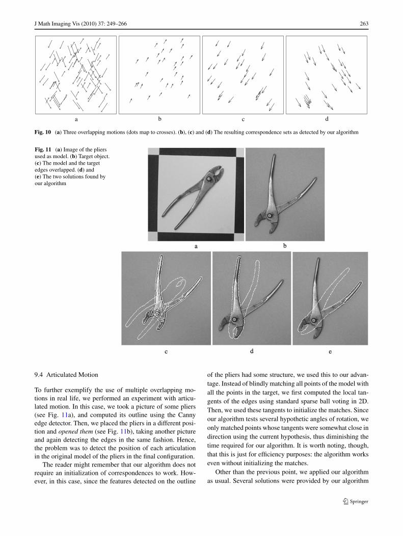
Fig. 10 (a) Three overlapping motions (dots map to crosses). (b), (c) and (d) The resulting correspondence sets as detected by our algorithm
Fig. 11 (a) Image of the pliersused as model. (b) Target object.(c) The model and the targetedges overlapped. (d) and(e) The two solutions found byour algorithm
9.4 Articulated Motion
To further exemplify the use of multiple overlapping mo-tions in real life, we performed an experiment with articu-lated motion. In this case, we took a picture of some pliers(see Fig. 11a), and computed its outline using the Cannyedge detector. Then, we placed the pliers in a different posi-tion and opened them (see Fig. 11b), taking another pictureand again detecting the edges in the same fashion. Hence,the problem was to detect the position of each articulationin the original model of the pliers in the final configuration.
The reader might remember that our algorithm does notrequire an initialization of correspondences to work. How-ever, in this case, since the features detected on the outline
of the pliers had some structure, we used this to our advan-tage. Instead of blindly matching all points of the model withall the points in the target, we first computed the local tan-gents of the edges using standard sparse ball voting in 2D.Then, we used these tangents to initialize the matches. Sinceour algorithm tests several hypothetic angles of rotation, weonly matched points whose tangents were somewhat close indirection using the current hypothesis, thus diminishing thetime required for our algorithm. It is worth noting, though,that this is just for efficiency purposes: the algorithm workseven without initializing the matches.
Other than the previous point, we applied our algorithmas usual. Several solutions were provided by our algorithm
264 J Math Imaging Vis (2010) 37: 249–266
Fig. 12 (a) The set of pointsthat were applied a non-rigidtransformation (dots transformto crosses). (b) The curvesgenerated in the voting spaces.The arrows across the votingspaces show the localenforcement of the ReflectionConstraint. (c) Thecorrespondences found with ouralgorithm
at different angles. That is, for several hypothetic rotationangles, we found the position of both articulations of thepliers at the same time. However, we chose the solution thatyielded the highest number of matches for both articulationsat the same time. The original model of the pliers can beseen in Fig. 11a. The situation of the pliers after we rotatedand opened them can be seen in Fig. 11b. The edges of themodel and the target can be seen overlapped in Fig. 11c.The couple of positions found for each articulation of thepliers in the chosen solution can be seen in Fig. 11d and e.Note the large rotation present between the model and thetarget region (about 180°). It must also be mentioned thatin this experiment, we ran into another problem. A precisecorrespondence between the edges detected in each imagecannot be established, due to small differences in the “sam-pling rate”. Therefore, a fuzzy line was produced in the vot-ing spaces. To account for this inconvenience, we had to re-lax the thresholds for outlier rejection and uniqueness en-forcement. This, in turn, produced a few wrong or multiplematches in the end. However, since the vast majority of thecorrespondences were correct, the motion estimation algo-rithm was able to align the sets without further trouble. Inthis work, we have claimed that our algorithm has less prob-ability to be trapped in a local minimum, however in casesof pathological situations we should enforce to additionalconstrains to narrow down the search space, so that our algo-rithm is in a better position to chose the solution that yieldedthe highest number of matches.
9.5 Extension to Smooth 2D Non-rigid Motion
Our algorithm can also detect some instances of non-rigidmotion. Namely, those that still produce detectable curves inthe voting spaces. We have found that point sets that displaysmoothly-varying rigid transformations produce smoothcurves in the voting spaces. For example Fig. 12a displaysone such set. We generated this set by slowly varying therotation angle over the length of the string of points. Thevoting spaces display two clearly salient curves, as seen inFig. 12b.
In order to detect these curves, we employ the Algo-rithm 6.1. However, in the last stage, instead of globally en-forcing the reflection constraint of (35), we only require thateach token is locally consistent with this constraint acrossboth voting spaces, and reject the rest. This is illustrated inFig. 12b. Here we show two tokens along with their nor-mals, the arrows across the voting spaces show which tokensare used to enforce the Reflection Constraint locally. The re-sulting correspondences in this synthetic test are shown inFig. 12c.
10 Conclusions
We have presented a novel algorithm that combines thepower of expression of Geometric Algebra with the robust-ness of Tensor Voting to find the correspondences betweentwo sets of 2D points with an underlying rigid transforma-tion. This algorithm was also shown to work with excessiveamounts of outliers in both sets.
We have also used Geometric Algebra to derive a con-straint (35) that serves a double purpose: on one hand, it letsus decide whether or not the current lines correspond to arigid motion; and on the other hand, it allows us to rejectmultiple matches and enforce the uniqueness constraint.
Our algorithm does not require an initialization (thoughit can benefit from one). Works equally well for large andsmall motions. And can be easily extended to account formultiple overlapping motions and certain non-rigid transfor-mations.
It must be noted that our algorithms can detect multi-ple overlapping motions, whereas the current solutions onlywork for a single global motion. We have also shown thatour algorithm can work with data sets that present small non-rigid deformations.
In the unconstrained case, with a large amount of outliers(83–90%), our algorithm can take several minutes to fin-ish. However, in most real-life applications, these extremecircumstances are not found, and a good initialization can
J Math Imaging Vis (2010) 37: 249–266 265
Fig. 13 (a) A set of points X(circles) and the same set after arigid transformation has beenapplied Y (crosses). A tentativeset of correspondences betweenone point xi and the set Y isshown. (b) The same set, in thiscase, two points xi and xj arechosen and left fixed and all thepossible correspondences arethen considered (shown)
be computed. When these conditions are met, our algorithmcan be rather fast.
It is worth noting the effect of the “sampling rate” ofthe input points in our algorithm. Our method is based onan equation for point motion and assumes a direct point-to-point correspondence can be established. If the input datasets have been sampled at different rates, this condition willnot be met and the performance of our algorithm will de-grade, maybe even stop working altogether. We are currentlyworking on ways to overcome this problem.
10.1 Final Thoughts
It has come to our attention one interesting fact. The gen-eral correspondences problem might be considered as an NPproblem, since it consists of two parts: the non-deterministicgeneration of a set of correspondences, and the testing of thecorrectness of the set. In our particular case, the complexityof the problem is reduced significantly by using the extrainformation that a rigid transformation has taken place. Thisalone serves to diminish the complexity of the problem fromNP to P time.
Now, assume we have two sets of points X and Y. Foreach xi ∈ X there is one, and only one yj ∈ Y such that yi =Hxj , where H is 2D rigid transformation consisting of anarbitrarily large rotation and translation. We are expected tofind the correspondences mapping X to Y via H.
The naive approach to solve this problem would be asfollows: generate a tentative correspondences set betweenX and Y, compute the H generated by this set and test ifthe points X are actually mapped to the points Y. The non-deterministic part of the algorithm is the generation of thecorrespondences set. However, this can be easily formulatedin a systematic fashion and, since we are dealing with a 2Drigid transformation, the set does not need to comprise allthe points in X, but only enough to account for the threedegrees of freedom of H (two points).
The algorithm to choose the correspondences may pro-ceed as follows. Select xi ∈ X for each i = 1, . . . , n wheren is the number of points in X. For each xi chosen, select a
tentative corresponding point yj ∈ Y for each j = 1, . . . , n,where again, n is the number of points in Y (see Fig. 13a).This can be easily coded with two nested iterations, one toiterate over i and the other to iterate over j . The total num-ber of possible selections is therefore O(n2). Now, if weconsider that we need two such correspondences, it is evi-dent that we must nest four iterations (two iterations for eachpair) and therefore the algorithm is O(n4) in the worst case.Since the computation of H given a set of tentative corre-spondences is of O(1), this does not increase the complexityof the problem.
This simple scheme can be further optimized. We canchoose two points xi and xj from X and leave them fixed.Then we can iterate over the possible selections of the cor-responding yi′ and yj ′ for these points (see Fig. 13b). Thisoperation is of O(n2) since only two cycles are nested, oneto iterate over i′ and another to iterate over j ′.
On the other hand, in current approaches like ICP, thegeneration of correspondences is much more efficient but isbased on the assumption that corresponding points are closeto each other. Therefore, algorithms like the ICP will notwork even in the absence of outliers if the transformation islarge. Another problem of the ICP is that the solution pro-duced is highly dependent on the quality of the initialization.This algorithm might become trapped in a “local minimum”and thus might not produce the desired answer.
We have already shown that our algorithm is of O(nm) <
O(n2) where m < n is the number of neighbors that receivevotes from the current token. The reader might rememberthat we also proposed a hypothesize-and-test scheme wheredifferent skewing angles were tested in a systematic fashion.However, we must stress that when no outliers are present,we can detect the correct transformation without skewingthe space regardless of the magnitude of the transformation(see Fig. 5 for an example of this). Hence, no extra iterationsare needed, and our algorithm does provide a real decreasein computational costs. This has been possible because wehave re-cast the correspondences problem into another spacewhere a particular constraint of the problem was more read-ily detected and exploited. It is interesting to note that thisspace was found by using the Geometric Algebra.
266 J Math Imaging Vis (2010) 37: 249–266
Finally, we have discussed how a general NP problemcould be solved using a simple algorithm that runs in Ptime thanks to the use of extra knowledge that constrainsthe problem. Namely, that a rigid transformation has takenplace between the sets we must match. This same constraintis not properly exploited by other algorithms that also solvethis problem. In the case of ICP, for example, the problemis further limited by bounding the magnitude of the trans-formation to a relatively small range. In our case, we haveapplied a transformation to the problem, taking it into an-other space where the aforementioned constraint is readilydetectable, without introducing extra limitations to the prob-lem (like bounding the magnitude of the transformation).Thus producing a more efficient algorithm by exploiting thispowerful constraint.
References
1. Bayro-Corrochano, E., Rivera-Rovelo, J.: The use of geometricalgebra for 3d modelling and registration of medical data. Int. J.Math. Imaging Vis. 34(1), 48–60 (2009)
2. Besl, P.J., McKay, N.: A method for registration of 3-d shapes.IEEE Trans. Pattern Anal. Mach. Intell. 14(2), 239–256 (1992)
4. Champleboux, G., Lavallée, S., Szeliski, R., Brunnie, L.: Fromaccurate range imaging sensor calibration to accurate model-based3d subject localization. In: IEEE Conference on Computer Visionand Pattern Recognition, pp. 83–89 (1992)
5. Chui, H., Rangarajan, A.: A new point matching algorithm fornon-rigid registration. In: IEEE Conference on Computer Visionand Pattern Recognition (CVPR), vol. 2, pp. 44–51 (2000)
6. Cunnington, S.J., Stoddart, A.J.: N-view point set registration:a comparison. In: British Machine Vision Conference, pp. 234–244 (1999)
7. Eggert, D., Fitzgibbon, A., Fisher, R.: Simultaneous registrationof multiple range views satisfying global consistency constraintsfor use in reverse engineering. Comput. Vis. Image Underst. 69,253–272 (1998)
8. Feldmar, J., Malandain, G., Declerck, J., Ayache, N.: Extensionof the icp algorithm to non-rigid intensity-based registration of 3dvolumes. In: Workshop on Mathematical Methods in BiomedicalImage Analysis, pp. 84–93 (1996)
9. Fitzgibbon, A.W.: Robust registration of 2d and 3d point sets. Im-age Vis. Comput. 21, 1145–1153 (2003)
10. Fookes, C., Williams, J., Bennamoun, M.: Global 3d rigid regis-tration of medical images. In: International Conference on ImageProcessing, vol. 2, pp. 447–450 (2000)
11. Grimson, W., Lozano-Pérez, T., Wells, W., Ettinger, G., White,S., Kikinis, R.: An automatic registration method for frameless
stereotaxy, image-guided surgery, and enhanced reality visualiza-tion. In: IEEE Conference on Computer Vision and Pattern Recog-nition, pp. 430–436 (1994)
12. Guest, E., Berry, E., Baldock, R., Fidrich, M., Smith, M.: Robustpoint correspondence applied to two- and three-dimensional im-age registration. IEEE Trans. Pattern Anal. Mach. Intell. 23(2),165–179 (2001)
13. Hestenes, D.: Space-Time Algebra. Gordon and Breach, NewYork (1966)
14. Ionescu, D., Abdelsayed, S., Goodenough, D.: A registration andmatching method for remote sensing images. In: Canadian Confer-ence on Electrical and Computer Engineering, vol. 2, pp. 710–712(1993)
15. Johnson, A., Kange, S.: Registration and integration of textured3d data. In: 3DIM’97, pp. 234–241 (1997)
16. Kalviainen, H., Oja, E., Xu, L.: Randomized hough transform ap-plied to translational and rotational motion analysis. In: 11th IAPRInternational Conference on Pattern Recognition, Conference A:Computer Vision and Applications, vol. 1, pp. 672–675 (1992)
17. Kang, E.Y., Cohen, I., Medioni, G.: Robust affine motion estima-tion in joint image space using tensor voting. In: 16th InternationalConference on Pattern Recognition, vol. 4, pp. 256–259 (2002)
19. Lu, F., Milios, E.: Robot pose estimation in unknown environ-ments by matching 2d range scans. In: Conference on ComputerVision and Pattern Recognition, pp. 935–938 (1994)
20. Luo, B., Hancock, E.: Matching point-sets using Procrustes align-ment and the em algorithm. In: 10th British Machine Vision Con-ference, pp. 43–52 (1999)
21. Medioni, G., Lee, M., Tang, C.: A Computational Frameworkfor Segmentation and Grouping. Elsevier Science, Amsterdam(2000)
22. Parka, W., Yan, L., Zhoua, Y., Mosesa, M., Chirikjian, G.: Kine-matic state estimation and motion planing for stochastic nonholo-nomic systems using the exponential map. J. Robot. 26
23. Reyes, L., Medioni, G., Bayro-Corrochano, E.: Registration of 3dpoints using geometric algebra and tensor voting. Int. J. Comput.Vis. 75(1), 67–92 (2007)
24. Simon, D., Herbert, M., Kanade, T.: Techniques for fast and ac-curate intra-surgical registration. J. Image Guid. Surg. 1(1), 17–29(1995)
25. Stoddart, A., Hilton, A.: Registration of multiple point sets. In:Proceedings of the International Conference on Pattern Recogni-tion, pp. 40–44 (1996)
26. Turk, G., Levoy, M.: Zippered polygons meshes from range im-ages. In: ACM SIGGRAPH Conference on Computer Graphics,pp. 311–318 (1994)
27. Wells, W.: Statistical approaches to feature-based object recogni-tion. Int. J. Comput. Vis. 21, 63–98 (1997)
28. You, J., Zhu, W., Pissaloux, E., Cohen, H.: Hierarchical imagematching: A chamfer matching algorithm using interesting points.In: Third Australian and New Zealand Conference on IntelligentInformation Systems, pp. 70–75 (1995)
29. Zhang, Z.: Iterative point matching for registration of free-formcurves. Technical Report 1658, INRIA (1992)


![[52] Sarvajit S. Sinha and Brian G. Schunck …iris.usc.edu/Outlines/papers/1995/liao-paper-95.pdf · [54] Stoer, J., and Bulirsch, R. 1980, inIntroduction to Numerical Analysis (New](https://static.documents.pub/doc/80x56/5b91ba6509d3f2f8508c3b98/52-sarvajit-s-sinha-and-brian-g-schunck-irisusceduoutlinespapers1995liao-paper-95pdf.jpg)


