36
Regularization Yow-Bang (Darren) Wang 8/1/2013
| Date post: | 13-Apr-2017 |
| Category: |
Technology |
| Upload: | yow-bang-darren-wang |
| View: | 254 times |
| Download: | 0 times |

RegularizationYow-Bang (Darren) Wang8/1/2013
Outline● VC dimension & VC bound – Frequentist viewpoint
● L1 regularization – An intuitive interpretation
● Model parameter prior – Bayesian viewpoint
● Early stopping – Also a regularization
● Conclusion

VC dimension & VC bound – Frequentist viewpoint

Regularization● (My) definition: Techniques to prevent overfitting
● Frequentists’ viewpoint:
○ Regularization = suppress model complexity
○ “Usually” done by inserting a term representing model complexity into the objective function:
Training error
Model complexity
Trade-off weight

VC dimension & VC bound● Why suppressing model complexity?
○ A theoretical bound of testing error, called Vapnik–Chervonenkis (VC) bound, state the follows:
● To reduce the testing error, we prefer:○ Low training error ( Etrain ↓)○ Big data ( N ↑)○ Low model complexity ( dVC ↓)

VC dimension & VC bound● : VC dimension
○ We say a hypothesis set H has iff given # of instances ≤ N, there exists a certain
set of instances that can be binary-classified into any combination of class labels by H.
● Example: H = {straight lines in 2D space}
Label=1
Label=0
Label=1
Label=0
Label=1
Label=0
……
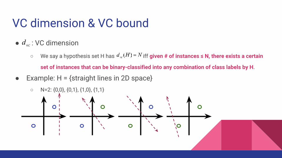
VC dimension & VC bound● : VC dimension
○ We say a hypothesis set H has iff given # of instances ≤ N, there exists a certain
set of instances that can be binary-classified into any combination of class labels by H.
● Example: H = {straight lines in 2D space}○ N=2: {0,0}, {0,1}, {1,0}, {1,1}

VC dimension & VC bound● : VC dimension
○ We say a hypothesis set H has iff given # of instances ≤ N, there exists a certain
set of instances that can be binary-classified into any combination of class labels by H.
● Example: H = {straight lines in 2D space}○ N=2: {0,0}, {0,1}, {1,0}, {1,1}
○ N=3: {0,0,0}, {0,0,1},……, {1,1,1}
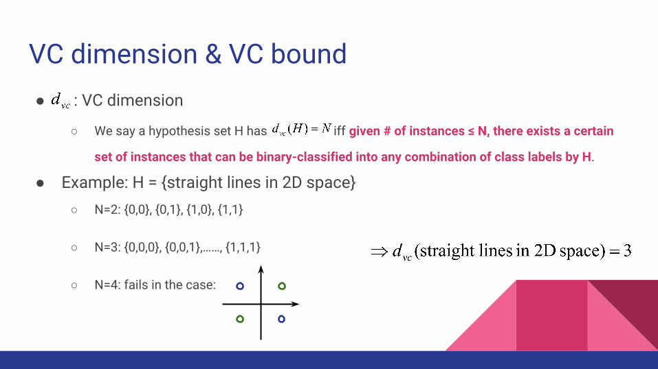
○ N=4: fails in the case:

Regularization – Frequentist viewpoint● In general, more model parameters
↔ higher VC dimension
↔ higher model complexity
↔
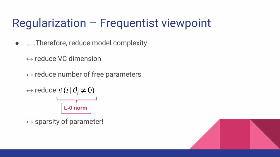
Regularization – Frequentist viewpoint● ……Therefore, reduce model complexity
↔ reduce VC dimension
↔ reduce number of free parameters
↔ reduce
↔ sparsity of parameter!
L-0 norm

Regularization – Frequentist viewpoint● The L-p norm of a K-dimensional vector x:
1. L-2 norm:
2. L-1 norm:
3. L-0 norm: defined as
4. L-∞ norm:

Regularization – Frequentist viewpoint● However, since L-0 norm is hard to incorporate into the objective function (∵
not continuous), we turn to the other more approachable L-p norms● E.g. Linear SVM:
● Linear SVM = Hinge loss + L-2 regularization!
L-2 regularization (a.k.a. Large Margin)Trade-off weight
Hinge Loss:

L1 regularization – An intuitive interpretation

L1 Regularization – An Intuitive Interpretation● Now we know we prefer sparse parameters
○ ↔ small L-0 norm
● ……but why people say minimizing L1 norm would introduce sparsity?
● “For most large underdetermined systems of linear equations, the minimal L1‐norm solution is also the sparsest solution”
○ Donoho, David L, Communications on pure and applied mathematics, 2006.

L1 Regularization – An Intuitive Interpretation● An intuitive interpretation: L-p norm ≣ control our preference to parameters
○ L-2 norm:
○ L-1 norm:
Equal-preferable lines
<Parameter Space>
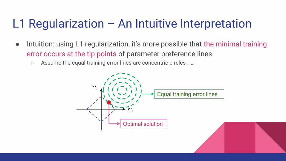
L1 Regularization – An Intuitive Interpretation● Intuition: using L1 regularization, it’s more possible that the minimal training
error occurs at the tip points of parameter preference lines○ Assume the equal training error lines are concentric circles ……
Equal training error lines
Optimal solution
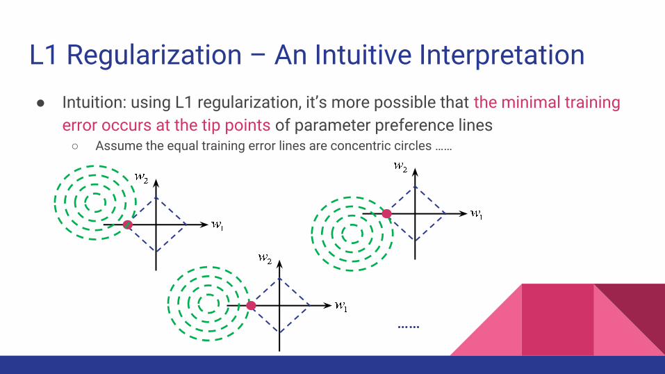
L1 Regularization – An Intuitive Interpretation● Intuition: using L1 regularization, it’s more possible that the minimal training
error occurs at the tip points of parameter preference lines○ Assume the equal training error lines are concentric circles ……
……

L1 Regularization – An Intuitive Interpretation● Intuition: using L1 regularization, it’s more possible that the minimal training
error occurs at the tip points of parameter preference lines○ Assume the equal training error lines are concentric circles, then the minimal training error
occurs at the tip points iff the centric of equal training error lines lies in the shaded areas as the figure shows, which is relatively highly probable!

Model parameter prior – Bayesian viewpoint

Regularization – Bayesian viewpoint● Bayesian: model parameters are probabilistic.
● Frequentist: model parameters are deterministic.
Given observation
Fixed yet unknown universeSampling
Estimate parameters
Unknown universe
Random observation
Sampling
Estimate parameters assuming the universe is a certain type of model
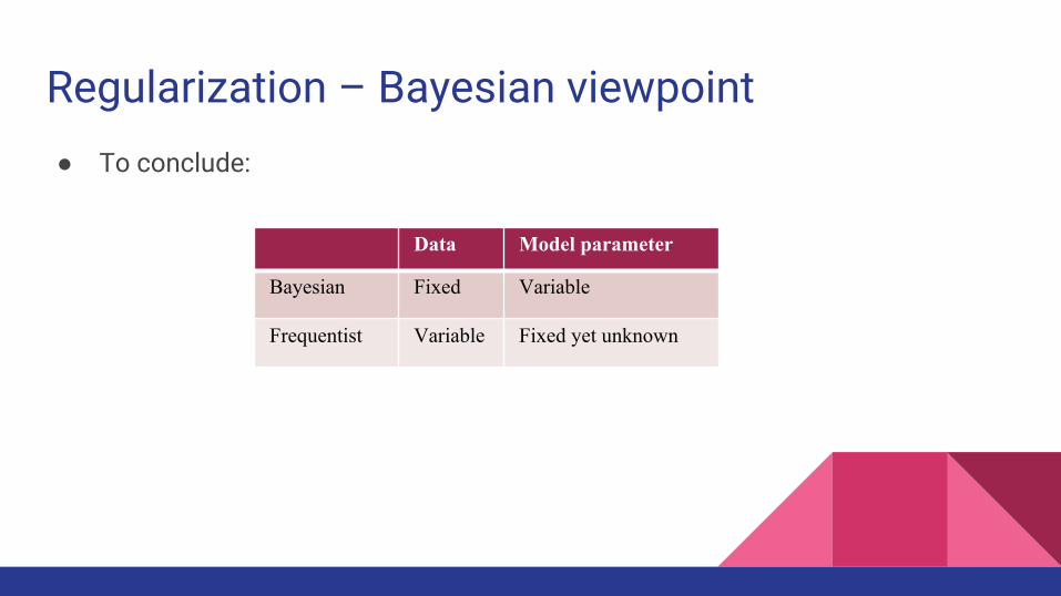
Regularization – Bayesian viewpoint● To conclude:
Data Model parameter
Bayesian Fixed Variable
Frequentist Variable Fixed yet unknown

Regularization – Bayesian viewpoint● E.g. L-2 regularization
● Assume the parameters w are from a Gaussian distribution with zero-mean, identity covariance:
<Parameter Probability Space>
Equal probability lines

Regularization – Bayesian viewpoint● E.g. L-2 regularization
● Assume the parameters w are from a Gaussian distribution with zero-mean, identity covariance:

Early stopping – Also a regularization

Early Stopping● Early stopping – stop training before optimal
● Often used in MLP training
● An intuitive interpretation:○ Training iteration ↑
○ → number of updates of weights ↑
○ → number of active (far from 0) weights ↑
○ → complexity ↑

Early Stopping● Theoretical proof:
○ Consider a perceptron with hinge loss:
○ Assume the optimal separating hyperplane is , with maximal margin
○ Denote the weight at t-th iteration as , with margin
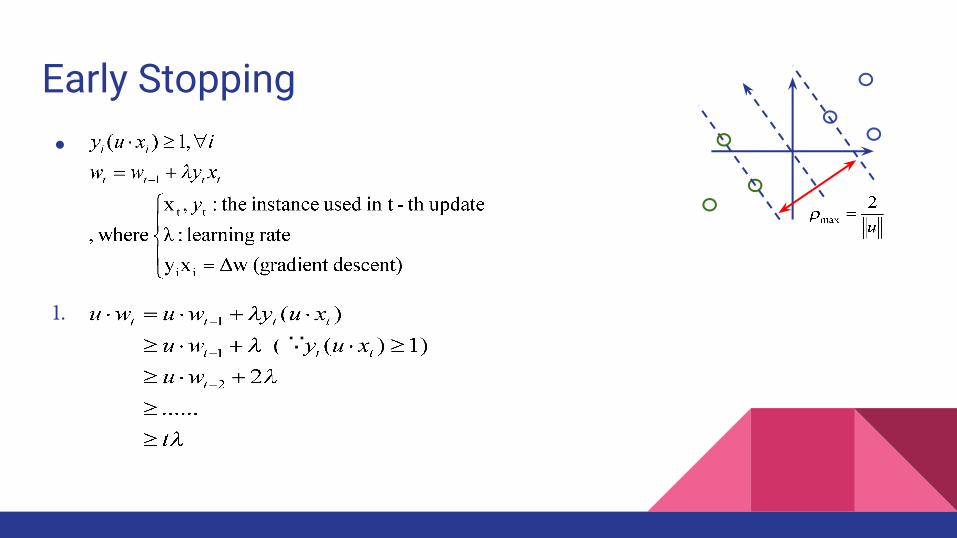
Early Stopping●
1.
∵
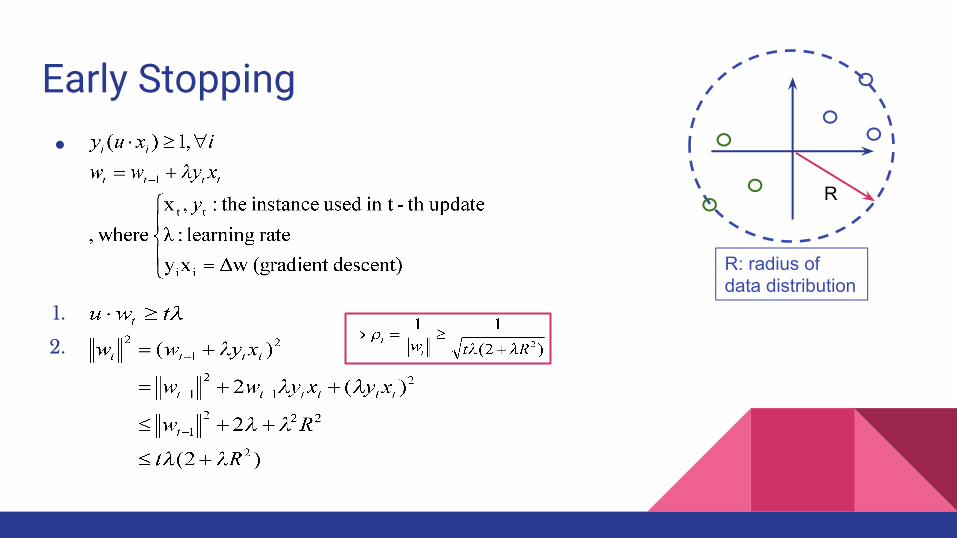
Early Stopping●
1.
2.
R: radius of data distribution
R

Early Stopping●
1.
2.
→
R: radius of data distribution
R
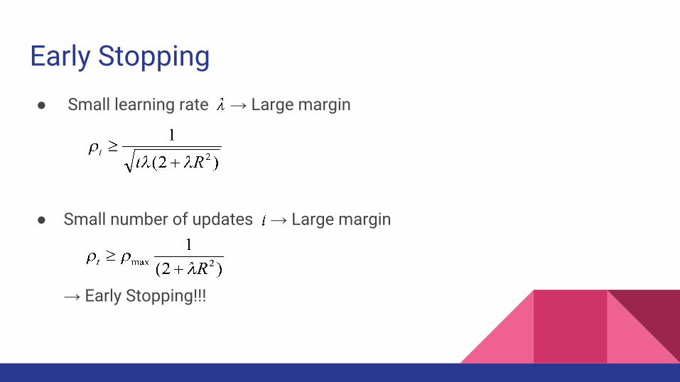
Early Stopping● Small learning rate → Large margin
● Small number of updates → Large margin
→ Early Stopping!!!

Early Stopping
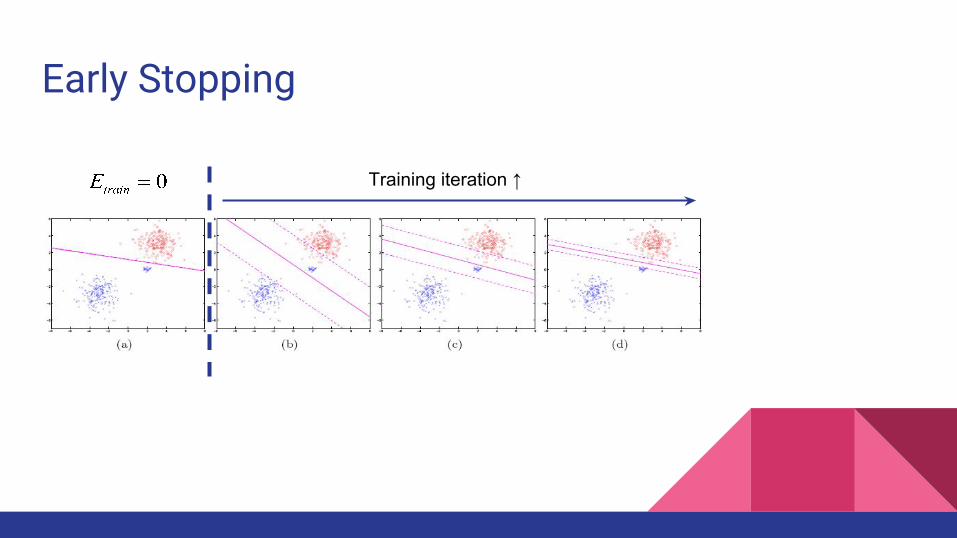
Early Stopping
Training iteration ↑

Conclusion

Conclusion● Regularization: Techniques to prevent overfitting
○ L1-norm: Sparsity of parameter○ L2-norm: Large Margin○ Early stopping○ ……etc.
● The philosophy of regularization○ Occam’s razor: “Entities must not be multiplied beyond necessity.”

Reference● Learning From Data - A Short Course
○ Yaser S. Abu-Mostafa, Malik Magdon-Ismail, Hsuan-Tien Lin
● Ronan Collobert, Samy Bengio, “Links Between Perceptrons, MLPs and SVMs”, in ACM 2004.


![WCDA Regularization for 3D Quantitative Microwave Tomography · WCDA Regularization for 3D Quantitative Microwave Tomography 2 problem is also ill-posed [11] and regularization is](https://static.documents.pub/doc/80x56/5e3abb0a2129886ec2199ead/wcda-regularization-for-3d-quantitative-microwave-tomography-wcda-regularization.jpg)


