1

Reinsurance Structure and Shareholder Value James Karim

August 2012

Introduction 1

Evaluating financing alternatives for an insurance company in a simplified model 2

Equity capital 2

Combination of equity and debt capital 3

Combination of equity capital and reinsurance 5

Illustration of the effect of reinsurance on equityholders’ return profile 7

Discussion and extensions to theoretical framework 15

Taxation 15

Bankruptcy costs 15

Multi-period insurance cashflows 16

Quantifying the effect of reinsurance structure on shareholder value 17

Appendix 1: Debt-to-equity and price-to-book ratios of selection of US P&C companies 19

Appendix 2: Financial data by company 20

References 21

1

Introduction

The value that an insurer’s decision to purchase reinsurance brings to a company can

only be measured on the scale of that company’s individual objectives. Whilst this

might seem like an obvious statement on the face of it, in fact many companies

struggle to be explicit about potentially contradictory corporate objectives. In this article,

we consider the position of a company that is purely seeking to maximise the market

value of its outstanding shares. This is a commercial goal that is fundamental for most

public companies.

At any given time, the value of a company’s shares will represent the expected NPV of

its dividend stream, evaluated at a discount rate reflecting the perceived riskiness of

the cashflows. The value of the dividend stream can in turn be maximised by

maximising the NPV of the firm’s corporate activities. This evaluation is our focus

below.

Questions relating to the amount of capital an insurer should hold are not addressed in

this article. In practice, this is a complex decision that will need to allow for pricing

implications of the company’s financial strength, regulatory and rating agency

considerations, as well as the potential costs of raising additional capital in a post-loss

environment - see Froot (2007).

In this article, we therefore take the decision as to capital quantum as a given, with our

analysis focussed upon a consideration of the relative merits of reinsurance and

traditional capital sources (i.e. debt and equity) for meeting the target funding level.

While reinsurance involves paying upfront for a promise of loss-contingent funding –

the opposite of equity and debt, where financing is given upfront and it is the return that

is contingent – it is a genuine capital substitute and can be incorporated within

conventional finance frameworks.

ABSTRACT

This article uses traditional corporate finance techniques to develop a methodology for the

economic valuation of reinsurance purchase. The issues are illustrated from the

perspective of a public company wishing solely to maximise the market value of its

outstanding shares. The company can do this by maximising the net present value

(“NPV”) of operations at its weighted average cost of capital (“WACC”). We demonstrate

below that reinsurance may affect not just operational cashflows, but also the WACC itself.

Previously, the latter effect has been accorded little attention, but as we show in this

article, it may well form the primary motivation for some reinsurance hedging. The NPV

framework unifies valuation issues surrounding earnings stability and capital relief and is

naturally suited to both short-and-long-tailed insurance lines of business. Using empirical

data, we show how the theory can be applied directly to infer the effects of reinsurance

purchase on company share valuations.

2

Equity capital

Let us assume a simplified world, in which a

new insurance company, initially funded with

100% equity capital, is characterised by the

following cashflows:

Time Description Cashflow

0 Initial equity injection – K

0 Receipt of premiums + P

0 Establishment of claim reserves

– P

– K

1 Payment of claims – C

1 Release of claim reserves + P

1 Release of tied up equity + K

P + K – C

We have omitted expenses, investment

income and frictional costs such as taxation

for simplicity. The highly stylised nature of

this example helps to draw out the key

insights, with practical extensions discussed

further below. The expected net present

value of this company’s operations is given

by the following expression1.

The parameter i0 above is the company’s cost

of capital. In this example, with 100% equity

financing, i0 is also the company’s cost of

equity and thus the parameter via which we

take account of the riskiness of the

cashflows. The more uncertain the insurance

profit at time 1, the greater the discount we

apply to it. A zero NPV would imply that the

expected profitability was just sufficient to

compensate shareholders for the risks

assumed. A positive NPV would be indicative

of the creation of shareholder value.

1 Strictly, we should cap the cashflow at time 1 at a minimum of zero, reflecting the shareholders’ limited liability. We ignore this for simplicity, without prejudicing the conclusions

In well-functioning capital markets, investors’

buying and selling actions influence the share

price so that the NPV of share purchase at

the appropriate discount rate is zero in

equilibrium. Consequently, no sooner is

shareholder value created, than the share

price is correspondingly bid upwards. This

instant recognition of the value operates to

return the NPV of share purchase to zero.

In the context of this example, if the firm’s

prospects are seen to offer exceptional value,

the second term on the right hand side of (1)

will grow beyond K and the market value of

the firm’s shares will exceed the book value

of K. We set out below empirical backup for

the notion that insurers generating returns in

excess of the cost of capital are valued more

highly by equity markets.

For the illustration of the basic theory, we

assume that initial equilibrium for the model

company sees prospective returns equal to

the cost of capital: In other words, the market

value of the firm equals its book value and

NPV0 above is zero.

We are assuming in this example that

equityholders are risk averse and demand a

risk premium for assuming insurance risk.

This could come about in a Capital-Asset-

Pricing-Model (“CAPM”) compliant world if

insurance companies’ risks were to some

extent non-diversifiable from broader equity

market risks - i.e. if insurance companies

have “β” parameters greater than zero. We

will demonstrate below that CAPM estimates

of the cost of equity for insurance companies

show risk premiums, with associated β

parameters being significantly positive.

NPV = – K +E (P – C + K)

1 + ioo

(1)

Evaluating financing alternatives for an insurance company in a simplified model

3

This may occur because insurance

companies themselves invest premiums and

surplus funds in positive β assets, or because

their liabilities share a correlation with market

risk. For example underwriters of trade credit

insurance may experience higher claims

during recessions or Financial Institutions

underwriters may find a correlation between

lawsuits and dislocations in financial markets.

However, we do not need to assume a world

where CAPM assumptions apply. Looking at

the coupons received by investors on

catastrophe bonds or the returns demanded

on sidecar investments, it would appear that

investors in these instruments require returns

in excess of risk free rates. This is observed

despite the fact that the underlying insurance

risk is generally catastrophe related and

broadly uncorrelated with market risk (zero

β). Either way, there is clear support for the

assumption of risk aversion amongst

investors in insurance-linked assets.

Combination of equity and debt capital

Whilst debt capital is not the primary focus of

this article, we develop some concepts below

that provide a foundation for an assessment

of reinsurance value.

Our company above may decide to consider

financing its operations in part by the

issuance of debt, which can be directly

substituted for equity. The debt would be

subordinate to the obligations to

policyholders. In this example, the company

still purchases no reinsurance.

Let us assume that an amount KD = K – KE is

raised as debt, where KE remains to be

financed as equity. The interest payable on

the debt is at a promised rate of r. Since debt

interest is a fixed cost, the equityholders here

are “gearing” their returns, amplifying their

returns in good times and their losses in bad

times.

In the revised capital structure, claim

liabilities will be paid firstly from policyholder

premiums, secondly from equity capital and

finally from debt capital.

As the equityholders have now taken a “first-

loss” position, the debtholders are a step

further removed from losses. This means that

the equityholders are carrying more risk per

unit of their investment. Consequently they

will require a greater return.

Modigliani and Miller (“MM”: see Modigliani

and Miller, 1958) demonstrated that capital

structure has no impact on the value of a firm

in a world of seamless capital markets and

devoid of frictional costs. Formally, they

argued that individual shareholders could

borrow or lend on their own accounts in a

way that would generate or remove leverage

as they desired. As such they could replicate

or undo the effects of borrowing by the firm,

meaning that no value would be created by

the firm doing this on their behalf.

More intuitively, we can say that capital

structure does not change the activities of the

firm. For a given set of investment decisions

– which for our company would be

underwriting insurance contracts - changing

capital structure is merely redefining the

division of the spoils. The value is generated

by the selection of insurance contracts

written, rather than by how the resulting

profits are divided among the parties who put

up the finance. The division of these profits is

a zero-sum game.

Looking specifically at the equityholders in

the newly-levered firm, their expected NPV is

given by:

NPV = – K +

E (P – C – rK + K )1 + iE E

E

D E (2)

4

We described above how NPV0 is zero in

equilibrium, when the activities of the firm

earn just enough margin to meet the cost of

equity. But what would it take to make NPVE

positive, having modified the capital

structure?

The right-hand-side will be positive and thus

the equityholders will gain financially from the

debt-for-equity swap if:

Intuitively, if the cost of equity is less than the

expected return on equity, the equityholders

gain. However, in efficient capital markets,

the debtholders’ required interest return will

leave just enough of the pie remaining for

equityholders to meet their necessary return -

but no more. In other words:

Observing that NPV0 is zero in (1), we can

rewrite this as the more conventional

expression of MM’s second proposition:

The right hand side is usually termed the

weighted average cost of capital (“WACC”).

E(r) here is interpreted as the cost of debt or

the expected return to debtholders. Where

there is a risk of default on cashflows due to

the debtholders, E(r) is lower than the

promised rate of interest, r. MM’s second

proposition tells us that, absent capital

market inefficiencies and frictional costs, the

WACC is invariant to capital structure.

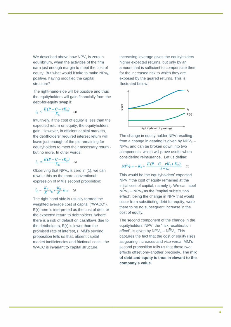
Increasing leverage gives the equityholders

higher expected returns, but only by an

amount that is sufficient to compensate them

for the increased risk to which they are

exposed by the geared returns. This is

illustrated below:

The change in equity holder NPV resulting

from a change in gearing is given by NPVE –

NPV0 and can be broken down into two

components, which will prove useful when

considering reinsurance. Let us define:

This would be the equityholders’ expected

NPV if the cost of equity remained at the

initial cost of capital, namely i0. We can label

NPVE – NPV0 as the “capital substitution

effect”, being the change in NPV that would

occur from substituting debt for equity, were

there to be no subsequent increase in the

cost of equity.

The second component of the change in the

equityholders’ NPV, the “risk recalibration

effect”, is given by NPVE – NPVE. This

captures the fact that the cost of equity rises

as gearing increases and vice versa. MM’s

second proposition tells us that these two

effects offset one-another precisely. The mix

of debt and equity is thus irrelevant to the

company’s value.

i <E (P – C – rK )

KEE

D(3)

i =E (P – C – rK )

KEE

D(4)

i =KKE io E

+KKD E (r) (5)

Re

turn

KD / KE (level of gearing)

ie

i0

E(r)

NPV = – K +E (P – C – rK + K )

1 + iE ED E

o

^(6)

^

^

5

Combination of equity capital and reinsurance

The first question to be asked is whether, in a

world free of capital market distortions and

frictional costs, MM’s propositions would

negate the need to evaluate reinsurance

strategy. Could we use the argument above

that the parties’ claims on the company’s

assets merely adjust themselves to reflect the

relative risk positions assumed, such that the

mix between equity and reinsurance is

irrelevant? If so, we could move directly to

the issue of how to consider adjusting MM’s

propositions in a world featuring the

distortions we have assumed away.

The idea of MM irrelevance may be less

intuitive in a reinsurance context. This is

partly because of the reversal of the

investment and return cashflows: with

reinsurance, the investment (the recovery) is

contingent and payable after the loss event,

with the return (the reinsurance premium)

payable upfront. However, this does not

prevent us from calculating the amount of

reinsurance capital sourced, nor its cost, as

we show below.

Another sense in which reinsurance feels at

odds with an equity/debt framework is that its

location in the capital structure is hard to

pinpoint. With the exception of whole account

aggregate stop loss, which is rarely bought or

available, reinsurance permeates the capital

structure. It is everywhere, but nowhere that

can be pinpointed precisely. Fortunately,

many reinsurance structures act either to

generate or to remove leverage, and so can

be accommodated within the developed

framework.

The key reason why we should not just

assume that MM will apply in a reinsurance

context is that reinsurance markets do not

behave identically to the capital markets:-

Unlike the equity and debt securities

issued by large companies, reinsurance

may be available from a small number of

sellers and is untraded. For some classes

and types of reinsurance, there may even

only be a single seller, meaning that the

mechanism by which the scrutiny of

thousands of investors drives a price to its

“fair” value is removed;

Reinsurers are professional risk

diversifiers. This opens up a possible

asymmetry in the cost of a particular risk

between cedant and reinsurer and thus an

opportunity for mutual benefit from a

reinsurance transaction. The zero-sum

game described above between debt and

equityholders may not be present here;

and

Reinsurance may be subject to pricing

cycles (“soft” and “hard” markets), which

means that short-run reinsurance

economics fluctuate and are worthy of

analysis

Given these important considerations, the

Reinsurance Manager has a valuable role to

play by incorporating reinsurance capital into

the firm’s financing structure in a manner that

improves the economics to equityholders.

To illustrate this further, suppose that the

ceded reinsurance premium is given by “X”

and the reinsurance recoveries are given by

“R”. Let us assume further that the revised

equity requirement with the reinsurance

hedges in place is given by KRI. KRI may be

calculated after value-at-risk type risk

measures, more complex risk measures,

rating agency requirements or regulatory

factors have been taken into account.

The NPV for equityholders in a firm that

partially finances with reinsurance is:

NPV = – K +E (P – X – C + R + K )

1 + iRI RIRI

RI

(7)

6

Here, iRI represents the cost of equity with the

reinsurance programme in place. If NPVRI –

NPV0 is positive, changing the financing

structure to incorporate reinsurance will have

a positive payoff to the equityholders. By way

of analogy to (6) above, we can define:

The capital substitution effect resulting from a

reinsurance purchase is given by NPVRI –

NPV0 and will be positive if:

The expression on the left of (8) measures

the expected cost of reinsurance per unit of

equity capital saved and is akin to what is

sometimes termed “Ceded RoE”. This is the

first part of our analysis of the increase in

equityholders’ value from the purchase of

reinsurance.

Where the reinsurance purchase leaves the

equityholders’ risk profile unchanged - i.e.

where the risk recalibration effect is zero and

i0 = iRI - this provides a complete picture of

the changes in NPV. In all other cases, we

need a means of trying to assess the impact

of reinsurance changes on the cost of equity

itself. This is a problem which we address

below.

Intuitively, reinsurance can change

shareholder value by reducing the overall

cost of financing the company’s operations. It

does not directly influence the insurance

contracts written, but may allow them to be

written more efficiently. We discuss this

notion of efficiency further, but an important

observation at this stage is that the right hand

side of (7) will be positive and the

reinsurance will add shareholder value if:

The left hand side of (10) is an expression for

the WACC when capital is provided by a

mixture of reinsurance and equity. The first

term can be thought of as the cost of

reinsurance capital. The reinsurance

structure will add value if it reduces the

WACC from its initial starting value of i0.

There is a one-to-one link between increasing

NPV and reducing WACC. They are flipsides

of the same coin.

NPV = – K +^

RI RI

E (P – X – C + R + K )1 + i

RI

o(8)

E (X – R)K – KRI

< io (9)

E (X – R)K – KRI

*K – K

KRI + i

RI

KK

RI < io (10)

^

7

Overleaf, we illustrate equityholder return

profiles for different financing alternatives. A

model insurance company weighing up its

funding options is modelled as having a

combined ratio with mean 85% and standard

deviation 27.5% and seeks to capitalise itself

to the 1 in 500 value at risk (net of any

reinsurance). In the gross case, this requires

capital of 100% of gross written premium.

Figure 1 shows the density function of the

equityholders’ internal rate of return, where

all cashflows are modelled as realised within

the first year for simplicity. Equityholders

have an expected return of 15%, which we

assume just sufficient.

In Figure 2, we can see the effect on the

equityholders’ return profile of refinancing

50% of the equity with debt. The debt interest

rate here is set at 8%, with a probability of

attachment of 2.6%. This generates an

expected return to the debtholders of 6.8%.

The gearing effect increases the

equityholders’ expected IRR, but the spread

of returns is now considerably greater. Note

the probability mass at a minus 100% return,

when all the equity is burned through, and the

debtholders start paying claims. The chance

of losing the entire equity investment has

increased by a factor of 15.

As explained above, if the MM result is taken

as broadly applicable – we set out more

below on how reasonable this is – and on the

assumption that the debt cost is fair, the

equityholders are indifferent between these

two investment profiles. The increase in

expected return from 15% to 23%

compensates them just sufficiently, but not

excessively, for the increase in risk assumed.

The change in capital structure has left their

value position unchanged.

In Figures 3 and 4, we consider the purchase

of stop loss reinsurance. The stop loss in

Figure 3 attaches at a combined ratio of

146% and exhausts at 200% for a premium

of 4% (or 7.4% rate on line). Since the

premium of 4% is payable upfront (unlike a

debt interest payment, which may be

defaulted upon), the capital relief provided by

this contract is 50% of gross premium.

Another way of saying this is that equity of

50% of gross premium must be raised to pay

the stop loss premium and cover the risk of

the combined ratio being realised between

100% and 146%. This will ensure the 1 in

500 downside is just covered.

The remaining equity investment in Figure 3

has an identical payoff structure to that of the

levered equity position shown in Figure 2.

The stop loss mirrors the subordinated debt

precisely. As such, the value of purchasing

this stop loss must be the same as the value

of the refinancing carried out with debt in

Figure 2.

If MM is applicable, both have zero value.

Looking solely at the cost of the stop loss per

unit of equity capital saved is in isolation an

insufficient value metric. Whilst it is below the

WACC of 15%, this merely represents its

greater subordination in the capital structure.

We cannot judge value without considering

the knock-on effect on the post-reinsurance

cost of equity. To do so would be to accept

implicitly that a company can increase its

value merely by issuing more debt, a

conclusion that few CFOs would accept and

which we show later has no empirical

support.

On first glance, it can seem counter-intuitive

to think of reinsurance as potentially

increasing the cost of equity. Surely

reinsurance is about risk reduction? Isn’t risk

always lower with reinsurance?

In fact, a more accurate way to think about

reinsurance is as a risk transfer mechanism.

If we transfer the least risky parts of the

capital structure and retain the riskiest, then

Illustration of the effect of reinsurance on equityholders’ return profile

8

the risk per unit of the remaining investment

actually increases. We have already

illustrated this above with debt, where we

transferred the most remote risk to

debtholders, thus leaving behind a more

volatile risk.

Figure 4 shows an alternative stop loss,

representing a layer of 62.5% excess of

87.5% in combined ratio terms. The stop loss

premium here is 12.5% of gross premium (or

20% rate on line). The equityholders in this

example have effectively taken the claims-

paying position of the debtholders in Figure 2.

However, they receive all the upside profit

from the business. Their return is maintained

and their risk reduced. In the terminology

developed above, both capital substitution

and risk recalibration effects are positive. As

such, this contract would deliver tremendous

value to the company. Yet if we measure

value solely based on cost per unit of equity

capital relieved, it looks no different to the

prior stop loss we considered.

The final graphs (Figures 5 and 6) show the

effects of two different types of quota share

reinsurance. Figure 5 illustrates a traditional

quota share without override commission.

There is no leverage effect here; rather, we

are really just selling a (one-year) equity

stake in the company to a reinsurer. The

equityholders have the same return

distribution on a smaller investment. Their

cost of equity remains unchanged.

Conversely, the structured quota share to the

right has a long sliding scale commission,

such that the reinsurer starts losing money at

a remote combined ratio. We have designed

this contract so that the reinsurer faces a

loss-making position beyond a 150%

combined ratio.

While such an arrangement may raise

eyebrows, we have assumed for the purpose

of illustrating the theory that full capital relief

is available at the rate of cession. The

reinsurer here is putting itself in the position

of the debt investors in Figure 2. The

equityholders’ IRR distribution is halfway

(representing 50% cession) between the

cases shown in pictures 1 and 2. As the

cession rate increases to 100%, the

distribution converges to that seen in Figures

2 and 3.

Using the same argument as before, if MM

conditions hold, this quota share generates

no value, even though the cost per unit of

released equity is low. There is a negative

risk recalibration effect to be taken into

account: the cost of equity will go up as a

result of the leverage introduced.

Structured quota shares are common, but are

often valued simplistically in the same way as

traditional quota shares. This can lead to

misleading decision rules.

These examples have been designed to

highlight the key insights from above, rather

than to illustrate the most common

reinsurance structures placed. In the next

section, we look at some real world case

studies.

9

Figure. 1

100% Equity financing Figure. 2

50% Equity + 50% debt

Mean 15.13% Mean 23.48%

E(Return | Return < 0) -22.35% E(Return | Return < 0) -41.62%

75th %ile 0.09% 75th %ile -7.82%

90th %ile -20.75% 90th %ile -49.50%

95th %ile -36.51% 95th %ile -81.03%

Prob(-100%) 0.21% Prob(-100%) 3.16%

Equity Capital Saving N/A Equity Capital Saving 50

E(Ceded Profit) N/A E(Ceded Profit) 3.40

Cost per Unit Equity Saved N/A Cost per Unit Equity Saved 6.8%

Figure. 3

50% Equity + 50% stop loss (54% XS 146% combined ratio for premium of 4.00)

Figure. 4

50% Equity + 50% stop loss (62.5% XS 87.5% combined ratio for premium of 12.50)

Mean 23.48% Mean 23.42%

E(Return | Return < 0) -41.62% E(Return | Return < 0) -37.92%

75th %ile -7.82% 75th %ile 0.00%

90th %ile -49.50% 90th %ile 0.00%

95th %ile -81.03% 95th %ile 0.00%

Prob(-100%) 3.16% Prob(-100%) 0.21%

Equity Capital Saving 50 Equity Capital Saving 50

E(Ceded Profit) 3.40 E(Ceded Profit) 3.42

Cost per Unit Equity Saved 6.8% Cost per Unit Equity Saved 6.8%

-100% 0% 100% 200%

Equityholder IRR

-100% 0% 100% 200%

Equityholder IRR

-100% 0% 100% 200%

Equityholder IRR

-100% 0% 100% 200%

Equityholder IRR

10

Figure. 5

50% equity + 50% traditional quota share Figure. 6

50% equity + 50% structured quota share

Mean 15.13% Mean 17.91%

E(Return | Return < 0) -22.35% E(Return | Return < 0) -28.73%

75th %ile 0.09% 75th %ile -2.55%

90th %ile -20.75% 90th %ile -30.34%

95th %ile -36.51% 95th %ile -51.35%

Prob(-100%) 0.21% Prob(-100%) 0.21%

Equity Capital Saving 50.00 Equity Capital Saving 25.00

E(Ceded Profit) 7.57 E(Ceded Profit) 1.70

Cost per Unit Equity Saved 15.1% Cost per Unit Equity Saved 6.8%

-100% 0% 100% 200%

Equityholder IRR

-100% 0% 100% 200%

Equityholder IRR

11

Case Study 1 Reinsurance Programme Of Lloyd’s Syndicate

This Lloyd’s Syndicate has a variety of reinsurance structures that protect its gross

account. Reinsurance reduces its 1 in 200 net loss - which we are using as a proxy for the

capital requirement, ignoring the “Lloyd’s Uplift” and non-underwriting risk for simplicity -

from 86.5m to 31.1m. The gross return on equity would be 19.1% and we assume for

simplicity that this equals its cost. Effectively we are assuming for illustration purposes that

the book value of the company equals its market capitalisation.

The expected cost of the reinsurance capital, given by the left hand side of the inequality

marked (9) above (and sometimes termed “Ceded RoE”) is 14.9%, which is below the cost

of equity. Since the reinsurance capital costs less than the equity it replaces, this

generates a positive capital substitution effect. However, the graph overleaf demonstrates

clearly what has happened to the distribution of the equityholders’ return. The green line

shows how the equityholders’ IRR distribution would look if the business were 100%

equity funded. The dark blue line shows the distribution of equity returns after the

purchase of the reinsurance programme. It can be seen that this has a higher mean, up

from 19.1% to 26.5%, but with a much greater spread. The risk profile of the equity has

therefore increased, and we need to assess what this has done to the cost of equity. If we

accept that these equityholders are risk averse, the cost of equity must have risen from

19.1%.

Estimating the increase in the cost of equity is a tough proposition. In the situations above,

we were able to precisely replicate reinsurance structures with debt alternatives. Generally

speaking, in the absence of aggregate stop loss or contracts which operate in the same

way (such as some structured quota shares), we will need to make the best possible

approximation. This is likely to be more accurate than assuming no change in the cost of

equity at all.

Suppose that the company could swap 55% of its equity for debt and that this debt, with a

2.2% chance of attachment, would typically be priced at 8% in the fixed income capital

markets. If we apply MM’s second proposition, the cost of equity would then rise to 34.1%,

leaving the WACC unchanged at 19.1%. The return profile of the equityholders after this

hypothetical refinancing is shown by the light blue line in the graph overleaf. Its variability

is similar to that of the equityholders’ return after reinsurance. The lines are not a perfect

match: the light blue line is slightly tighter, but has a higher probability of total loss (i.e. -

100% return). We are required to trade these two types of risk against one other using no

more than intuition. But the light blue line is a less imperfect fit for the dark blue line than

the green line.

We can infer from this that the costs of equity under these two financing structures should

be similar. If we use 34.1% as the revised cost of equity for the structure involving

reinsurance purchase, we can see that the risk recalibration effect outweighs the capital

substitution effect. The overall effect of the reinsurances purchased by this Syndicate is to

increase the WACC and reduce shareholder value. Far from being disheartening, this

invites a more granular analysis to ascertain which contracts are generating the leverage -

and at what price.

Whereas a traditional reinsurance analysis looks at the marginal dollars of equity saved by

different structures, here we need to look at the marginal effects of different structures on

the cost of equity. By restructuring or removing the contracts leveraging equityholder

returns without sufficient reward, we can improve this Syndicate’s offering to shareholders.

In attempting to mirror the effect of reinsurance on equity returns, we considered a 55%

debt financing structure. The feasibility of such a high leverage ratio from a regulatory

perspective is not something that we need to worry about per se: it is only an obstacle

insofar as it renders the job of estimating a suitable debt interest rate more difficult. It is

worth pointing out here that this example highlights the ability of reinsurance to generate

leveraged returns when conventional methods may not be permissible.

12

Equity Equity + R/I Equity + Debt

Written Premium 123,400,000 105,800,000 123,400,000

Expense Ratio 8.00% 9.33% 8.00%

Return Period Capitalisation 200 200 200

Capital Requirement 86,488,606 86,488,606 86,488,606

Equity Capital 86,488,606 31,068,148 38,919,873

Debt Capital 0 0 47,568,733

Reinsurance Capital 0 55,420,458 0

Expected Equity IRR 19.07% 26.51% 34.13%

Debt Interest Rate 0.00% 0.00% 8.00%

Cost of Equity 19.07% 34.13% 34.13%

Cost of Debt 0.00% 0.00% 6.74%

Cost of Reinsurance Capital 0.00% 14.89% 0.00%

WACC 19.07% 21.80% 19.07%

Capital Substitution Effect (1) 0 1,941,463 4,924,257

Risk Recalibration Effect (2) 0 -3,707,402 -4,924,257

NPV of Change in Capital Structure = (1) + (2) 0 -1,765,939 0

NPV Change as % Company Gross Book Value 0.00% -2.04% 0.00%

Equityholder IRR WACC

-100% -50% 0% 50% 100% 150%

Equity IRR

Equity + R/I IRR

Equity + Debt IRR

0%

5%

10%

15%

20%

25%

Equity Equity + R/I

Risk RecalibrationCapital

Substitution

13

Case Study 2 Per risk reinsurance programme of direct US property insurer

This primary US Insurer (“ABC”) is exposed to property risk and Cat perils and is

considering the value of its risk excess of loss programme. Rather than looking at the

effect of a combination of programmes, as we did above, in this case we are looking at

one programme in isolation.

Here, the reinsurance structure actually decreases equityholder leverage slightly, rather

than increasing it. This can be seen in the graph on the exhibits page overleaf and may be

expected from a risk excess of loss structure. Noting this, we need to make subtle

changes to the approach used above in order to compute the two value effects that we

have developed.

Rather than considering notionally swapping debt for equity, we now need to consider the

opposite: ie notionally raising more equity capital than is required to run the insurance

company and then lending the excess capital to a similar company seeking leverage

(Company “XYZ”). It must be stressed that this is a purely conceptual exercise: we are

merely considering this course of action to compare the distribution of returns achievable

with those obtained from running ABC with its reinsurance programme.

If ABC raised an additional 12% capital, which it then proceeded to lend to XYZ in order to

assist XYZ in its 12% debt for equity swap, ABC would be dampening down the overall

risk of its investment portfolio. The return for this portfolio would be 14.2%, rather than the

15.1% receivable for pure investment in ABC’s own activities. So it would be taking a

lower return, but for a lower risk.

The return profile of this portfolio of two investments is comparable to the return for the

equityholders in ABC after reinsurance, as can be seen in the graph overleaf. Hence,

14.2% is a reasonable starting point for ABC’s post reinsurance cost of equity. We can

see this in the top graph, where the equityholder return profiles have the same risk and

return characteristics. Using this, we can see that, while the capital substitution effect is

negative, it is outweighed by the positive risk recalibration effect. ABC is adding more

value by reducing the volatility of equityholders’ returns than it is removing by replacing

equity with slightly more costly reinsurance. This highlights one of the key benefits of using

a joined-up, NPV-based approach to reinsurance valuation: we are explicitly able to value

reductions in earnings volatility. Under a more simplistic valuation framework, the

programme might be written off in light of every dollar of equity saving costing 18 cents, a

rate higher than the cost of capital.

14

Equity Equity + R/I Equity + Loan

Written Premium 280,000,000 259,300,000 280,000,000

Expense Ratio 30.00% 32.39% 30.00%

Return Period Capitalisation 200 200 200

Capital Requirement for Investments 128,523,626 128,523,626 143,946,461

Investment in ABC 128,523,626 110,164,189 128,523,626

Capital Loaned to XYZ 0 0 15,422,835

Reinsurance Capital 0 18,359,438 0

Expected IRR on Equity Investment in ABC 15.06% 14.46% 15.06%

Interest rate on Loan to XYZ 0.00% 0.00% 8.00%

Cost of Equity Investment in ABC 15.06% 14.22% 15.06%

Expected Return on Loan to XYZ 0.00% 0.00% 7.28%

Cost of Reinsurance Capital 0.00% 18.64% 0.00%

"WACC" 15.06% 14.85% 14.22%

Capital Substitution Effect (1) 0 -571,747 -

Risk Recalibration Effect (2) 0 798,848 -

NPV of Change in Capital Structure = (1) + (2) 0 227,101 -

NPV Change as % Company Gross Book Value 0.00% 0.18% -

Equityholder IRR WACC

-100% -50% 0% 50% 100% 150%

Equity IRR

Equity + R/I IRR

Equity + Loan IRR

0%

2%

4%

6%

8%

10%

12%

14%

16%

Equity Equity + R/I

Risk Recalibration

Capital

Substitution

15

Taxation

In our description of MM’s Proposition II, we

summarised the idea that capital structure

affects the division of returns between capital

providers, but not the returns themselves.

Hence, the WACC should not change with

capital structure: one party’s gain is another’s

loss.

In the real world, there may be third parties

who have an interest in the company’s

cashflows. A notable example would be the

tax authorities. It is typical that debt interest is

tax deductible, meaning that the taxman gets

a lower share of the company’s revenue as

the level of gearing rises: debt is more tax

efficient than equity. Ceded reinsurance

premiums are a tax deductible cost, meaning

that reinsurance shares the tax efficiency of

debt capital.

The simple framework used above can be

generalised: in computing the NPV of a

change in capital structure, we simply need to

consider the NPV of changes in taxation

payable, as well as the NPV of the other two

effects upon which we have focussed

primarily. In practice, we would need to take

all forms of taxation into account, including

the personal taxation of interest payments,

dividend payments and capital gains. If

capital gains are taxed at a lower rate or with

more favourable allowances, the tax benefits

of debt financing may be considerably

reduced.

Bankruptcy costs

Were the tax efficiency of debt without

opposing forces, the optimal capital structure

would involve minimising equity capital. In

practice, as the gearing of a firm increases,

the probability of its bankruptcy increases.

This increase may be negligible or modest at

first, but becomes overwhelming at very high

levels of gearing.

Bankruptcy is a costly process. The direct

costs of professional fees may be substantial,

but a high probability of bankruptcy carries

with it indirect costs, such as an inability to

retain staff or a distortion of the activities that

the firm takes on. Equityholders may take

excessively risky ventures in the knowledge

that they have minimal downside, but all the

upside.

The choice of optimal capital structure may

be described as finding the optimal balance

between these two effects. Estimating

bankruptcy costs is, regrettably, more

difficult.

It is important to stress that the framework

above does not rely on the acceptance of

MM. As long as we can value changes in

debt / equity policy and can mirror the payoffs

expected under different reinsurance

structures, we can place a value on those

structures.

We show in Appendix 1 that there is

significant variability of debt-to-equity ratios

among insurers and reinsurers. Were capital

structure to be crucial, one would expect a

greater degree of clustering around the

perceived optimum.

Discussion and extensions to theoretical framework

16

The regression line fitted in the left-hand box

of Appendix 1 shows a positive relationship

between the price-to-book ratio and the

degree of leverage. However, this is entirely

driven by the outlying Amtrust. There is good

reason to believe that Amtrust is valued

highly because its returns exceed its cost of

capital, rather than because shareholders are

attaching value to its high debt-to-equity ratio.

Without Amtrust, there is no significant

relationship and an R-squared of below 2%.

This is evidence to suggest that debt-to-

equity policies have little obvious and

consistent effect on value. Hence,

reinsurance valuation metrics should not

routinely ascribe value to capital structures

that are replicable via, and cost equivalent to,

the use of traditional capital sources.

This notion is not currently widely considered

by industry practitioners. We have shown

above that this can lead to potentially

misleading value decisions.

The full dataset is shown in Appendix 2.

Multi-period insurance cashflows

Our model of the insurance company was

considerably simplified in that we assumed all

cashflows happened at time zero or time 1. If

we have long-tailed lines of business, our

formula for the NPV of the company’s

operations (using equity financing) can be

rewritten as:

K0 here is the initial capital injection, with Kt

denoting the capital flow at time t, Ct the

claims paid at time t and Pt the premiums

received at time t. The other formulas can be

adjusted analogously. This is a considerable

advantage of using an NPV methodology

over a ratio-based approach, where allowing

for the tying up of capital over a multi-period

horizon is more challenging. Note that we are

not discounting any cashflows at the risk free

rate.

NPV = – K + ∑o ot

E (P – C + K )(1 + i )t t t

(11)

ot

17

The approach outlined above advocates

analysing the effect of reinsurance purchase

on the NPV of the company or, equivalently,

the WACC. The case studies showed how we

can put this into practice. We now consider

whether we can go one step further and

assess the implication for the company’s

share price of an improvement in its financing

efficiency.

One way of doing this would be purely

theoretical: we could calculate a theoretical

share price based on a simple discounted

dividend model. The standard formula

would be:

Here, P is the price of a share, D is the

dividend due next period, g the growth rate of

those dividends and i the cost of equity.

Using the techniques developed, we can

assess the impact on i of the reinsurance

purchase. We would also need to factor in

the change in D that may result in a greater

or lesser number of shares being in

circulation, as a result of the change in

financing structure.

However, this remains very theoretical and it

is difficult to apply sense-checking to any

proposed change in share price. An

alternative way of looking at the problem is to

look at a cross-section of company valuations

and see if the assumptions and implications

of the framework developed are supported.

We would expect to find that:

Those companies with future return

prospects in excess of their costs of equity

will trade above book value (and vice-

versa); and

The greater the excess of the expected

return over the cost of equity, the higher

the valuation

It is difficult to estimate objectively all the

future returns expected and to discount them.

Over a shorter horizon, however, we can look

at Analysts’ estimates for the 2013 return on

equity. Clearly this is a shorter term view of

value than would be ideal, but it is a useful

starting point.

In estimating each company’s cost of equity,

we have used the CAPM methodology

described above: we estimate each

company’s β based on its correlation with

broader (stock) market risk and add this

proportion of the market’s risk premium to the

risk free rate of return. The resulting

relationship for US insurance companies is

shown below, with the full dataset

summarised in Appendix 2.

The relationship is broadly as we would

expect to see. There are only 3 points in an

unexpected quadrant (circled in the graph),

where the price-book ratio is above 1, despite

a 2013 return that is expected to be below

the estimated cost of equity. There are many

possible reasons for this, but differences in

accounting methodologies, expectations of

merger activity and expectations of high

returns after 2013 are all possibilities.

The concave nature of the curve is what we

would expect to see if differential costs of

equity were the primary driver of different

valuations. In this case, we would expect the

Di – g

P = (12)

0.5

1.0

1.5

2.0

2.5

3.0

3.5

-10% -5% 0% 5% 10%

Pri

ce

/ B

oo

k R

atio

2013 Prospective RoE - Cost of Equity

Quantifying the effect of reinsurance structure on shareholder value

18

rate of descent of the curve to decline at low

valuations, as the company could always go

into run-off, placing a lower bound on the

discount to book value that could reasonably

apply. Here, the curve crosses at about 1.1,

close to the theoretical expectation of 1.

We demonstrate above how a change in

reinsurance structure may increase or

decrease the expected return on equity,

depending on whether the reinsurance adds

or removes leverage. We showed how to

estimate this change in the cost of equity,

and hence how to calculate the difference

between expected ROE and cost of equity

before and after changes in reinsurance

structure. We can thereby identify

reinsurance structures that move us North-

Eastwards along the valuation curve from our

starting position, towards higher share prices.

It is quite notable how relatively small

movements appear to offer the potential of

materially higher valuations. Looking at a

company with one of the lowest valuations,

XL Group, the valuation is severely impacted

by the high cost of equity. This may be

reduced by identifying and removing

reinsurances that are adding gearing, but for

little return, and by implementing

reinsurances that reduce earnings volatility

(see Case Study 2).

The relationship is less strong for the

reinsurers (see graph to right), where there is

a smaller sample and less variability.

However, the relationship is directionally as

one would expect. This adds support to the

idea that, if reinsurance can be used to

increase the spread between expected return

and cost of equity, equity valuations can be

increased.

R² = 0.5859

0.5

0.6

0.7

0.8

0.9

1.0

1.1

1.2

1.3

1.4

1.5

-5% 0% 5% 10%

Pri

ce

/ B

oo

k R

atio

2013 Prospective RoE - Cost of Equity

19

Including Amtrust Excluding Amtrust

Debt / Equity Ratio Debt / Equity Ratio

Mean 24.60% Mean 23.41%

Standard Deviation 14.18% Standard Deviation 12.22%

Minimum 2.30% Minimum 2.30%

Lower Quartile 15.15% Lower Quartile 15.13%

Median 23.00% Median 21.70%

Upper Quartile 30.90% Upper Quartile 29.30%

Maximum 70.00% Maximum 62.10%

R² = 0.3076

0.5

1.0

1.5

2.0

2.5

3.0

3.5

0% 20% 40% 60% 80%

Pri

ce

/ b

oo

k b

atio

Debt / equity ratio

R² = 0.0188

0.5

1.0

1.5

2.0

2.5

3.0

3.5

0% 20% 40% 60% 80%P

rice

/ b

oo

k r

atio

Debt / equity ratio

Appendix 1: Debt-to-equity and price-to-book ratios of selection of US P&C companies

20

Debt-to-Equity

Price / Book

Cost of Equity

Prospective 2013 RoE

Excess RoE

Insurer / Reinsurer

Ace 20.40% 1.23 9.60% 9.65% 0.05% Insurer

Alleghany 23.00% 1.02 7.60% 6.80% -0.80% Insurer

Allied World 24.60% 1.01 8.80% 7.39% -1.41% Insurer

American Financial Group 20.30% 0.84 9.40% Insurer

Amtrust 70.00% 3.06 9.80% 16.84% 7.04% Insurer

Arch 13.20% 7.20% 8.20% 1.00% Insurer

Argo 25.00% 0.64 8.20% 4.50% -3.70% Insurer

Chubb 23.10% 1.29 8.50% 10.00% 1.50% Insurer

Cincinnati 18.00% 1.17 9.20% 5.07% -4.13% Insurer

Employers * 26.20% 1.38 10.90% 8.04% -2.86% Insurer

Hanover Insurance Group 35.60% 0.72 8.80% 7.22% -1.58% Insurer

Loews 37.50% 0.87 10.40% 6.92% -3.48% Insurer

Markel 35.50% 1.58 8.00% 4.92% -3.08% Insurer

Navigators 14.00% 0.89 9.20% 4.95% -4.25% Insurer

Old Republic 24.10% 10.70% 12.46% Insurer

ProAssurance 2.30% 1.41 7.90% 9.00% 1.10% Insurer

RLI Corp 12.10% 1.92 8.30% 10.50% 2.20% Insurer

Selective 28.40% 0.9 9.70% 7.41% -2.29% Insurer

Tower 38.40% 1.2 8.60% 9.85% 1.25% Insurer

Travelers 26.60% 1.17 9.00% 9.48% 0.48% Insurer

United Fire 7.30% 0.79 9.90% 4.75% -5.15% Insurer

White Mountains ** 15.70% 0.95 7.50% 6.17% -1.33% Insurer

WR Berkley 52.40% 1.34 8.30% 9.20% 0.90% Insurer

XL Group 15.10% 0.69 14.50% 6.70% -7.80% Insurer

Alterra 15.40% 9.40% Reinsurer

Aspen 15.50% 0.75 8.60% 7.39% -1.21% Reinsurer

Axis 16.90% 0.83 8.80% 8.49% -0.31% Reinsurer

Bershire Hathaway 34.30% 9.10% Reinsurer

Endurance 19.60% 7.80% Reinsurer

Everest 12.90% 0.88 7.60% 10.40% 2.80% Reinsurer

Fairfax 36.00% 1.3 5.40% 8.70% 3.30% Reinsurer

Flagstone 29.60% 11.00% Reinsurer

Hannover Rueck 32.20% 12.60% Reinsurer

Muenchener Rueck 26.60% 11.90% Reinsurer

Partner Re 12.10% 0.91 8.30% 8.03% -0.27% Reinsurer

Platinum 14.60% 0.79 9.10% 6.80% -2.30% Reinsurer

Ren Re 7.70% 1.22 7.90% 13.40% 5.50% Reinsurer

Swiss Re 62.10% 12.50% Reinsurer

Validus 15.20% 0.96 8.10% 12.53% 4.43% Reinsurer

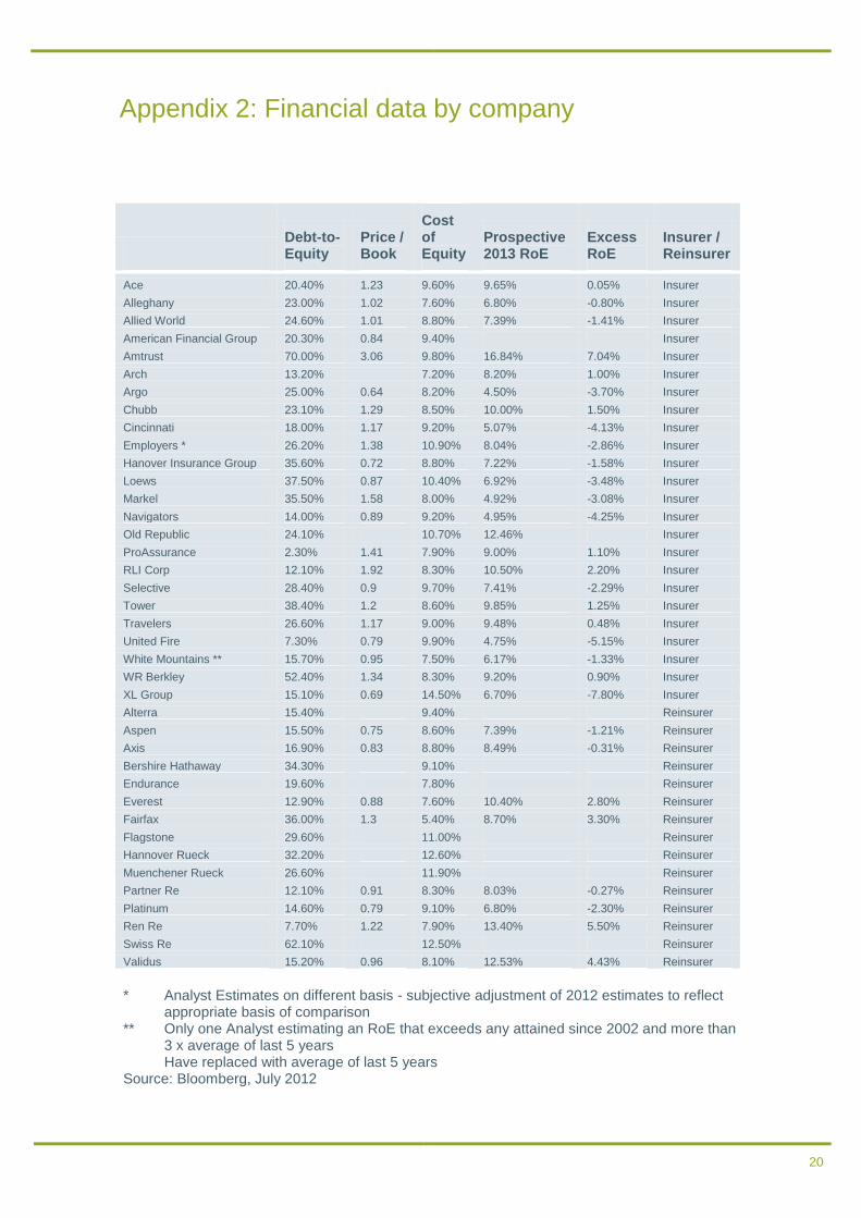
* Analyst Estimates on different basis - subjective adjustment of 2012 estimates to reflect

appropriate basis of comparison ** Only one Analyst estimating an RoE that exceeds any attained since 2002 and more than

3 x average of last 5 years Have replaced with average of last 5 years

Source: Bloomberg, July 2012

Appendix 2: Financial data by company

21

Froot, K.A, 2007, Risk Management, Capital Budgeting, and Capital Structure Policy for

Insurers and Reinsurers, Journal of Risk and Insurance, 74: 273-299

Modigliani, F.; Miller, M. (1958). "The Cost of Capital, Corporation Finance and the Theory of

Investment". American Economic Review 48 (3): 261–297

References