NCHRP Web Document 68 (Project 9-27) Relationships of HMA In-Place Air Voids, Lift Thickness, and Permeability Prepared for: National Cooperative Highway Research Program Submitted by: E. Ray Brown M. Rosli Hainin Allen Cooley Graham Hurley National Center for Asphalt Technology Auburn University Auburn, Alabama September 2004 Volume One
Transcript
NCHRP Web Document 68 (Project 9-27)
Relationships of HMA In-Place Air
Voids, Lift Thickness, and Permeability
Prepared for:
National Cooperative Highway Research Program
Submitted by:
E. Ray Brown
M. Rosli Hainin Allen Cooley
Graham Hurley National Center for Asphalt Technology
Auburn University Auburn, Alabama
September 2004
Volume One
ACKNOWLEDGMENT This work was sponsored by the American Association of State Highway and Transportation Officials (AASHTO), in cooperation with the Federal Highway Administration, and was conducted in the National Cooperative Highway Research Program (NCHRP), which is administered by the Transportation Research Board (TRB) of the National Academies.
DISCLAIMER The opinion and conclusions expressed or implied in the report are those of the research agency. They are not necessarily those of the TRB, the National Research Council, AASHTO, or the U.S. Government. This report has not been edited by TRB.
The National Academy of Sciences is a private, nonprofit, self-perpetuating society of distinguished scholars engaged in scientific and engineering research, dedicated to the furtherance of science and technology and to their use for the general welfare. On the authority of the charter granted to it by the Congress in 1863, the Academy has a mandate that requires it to advise the federal government on scientific and technical matters. Dr. Bruce M. Alberts is president of the National Academy of Sciences. The National Academy of Engineering was established in 1964, under the charter of the National Academy of Sciences, as a parallel organization of outstanding engineers. It is autonomous in its administration and in the selection of its members, sharing with the National Academy of Sciences the responsibility for advising the federal government. The National Academy of Engineering also sponsors engineering programs aimed at meeting national needs, encourages education and research, and recognizes the superior achievements of engineers. Dr. William A. Wulf is president of the National Academy of Engineering. The Institute of Medicine was established in 1970 by the National Academy of Sciences to secure the services of eminent members of appropriate professions in the examination of policy matters pertaining to the health of the public. The Institute acts under the responsibility given to the National Academy of Sciences by its congressional charter to be an adviser to the federal government and, on its own initiative, to identify issues of medical care, research, and education. Dr. Harvey V. Fineberg is president of the Institute of Medicine. The National Research Council was organized by the National Academy of Sciences in 1916 to associate the broad community of science and technology with the Academy’s purposes of furthering knowledge and advising the federal government. Functioning in accordance with general policies determined by the Academy, the Council has become the principal operating agency of both the National Academy of Sciences and the National Academy of Engineering in providing services to the government, the public, and the scientific and engineering communities. The Council is administered jointly by both the Academies and the Institute of Medicine. Dr. Bruce M. Alberts and Dr. William A. Wulf are chair and vice chair, respectively, of the National Research Council. The Transportation Research Board is a division of the National Research Council, which serves the National Academy of Sciences and the National Academy of Engineering. The Board’s mission is to promote innovation and progress in transportation through research. In an objective and interdisciplinary setting, the Board facilitates the sharing of information on transportation practice and policy by researchers and practitioners; stimulates research and offers research management services that promote technical excellence; provides expert advice on transportation policy and programs; and disseminates research results broadly and encourages their implementation. The Board's varied activities annually engage more than 5,000 engineers, scientists, and other transportation researchers and practitioners from the public and private sectors and academia, all of whom contribute their expertise in the public interest. The program is supported by state transportation departments, federal agencies including the component administrations of the U.S. Department of Transportation, and other organizations and individuals interested in the development of transportation. www.TRB.org
www.national-academies.org
i
TABLE OF CONTENTS
Page
LIST OF TABLES……………………………………………………………………………… iv
LIST OF FIGURES ..………………………………………...………………………...……… viii
1.0 INTRODUCTION AND PROBLEM STATEMENT…………………………………… 1
2.0 OBJECTIVE……………………………………………………………………………. 3
3.0 RESEARCH APPROACH………………………………………………………………. 3
3.1 Part 1 – Experimental Plan ……………………………………………………… 6
3.1.1 Evaluation of Effect of t/NMAS on Density Using
Gyratory Compactor…………………………………………………...… 6
3.1.2 Evaluation of Effect of t/NMAS on Density Using
Vibratory Compactor ……………………………………………………10
3.1.3 Evaluation of Effect of t/NMAS on Density Using Field Experiment.. ...11
3.1.4 Evaluation of Effect of Temperature on Relationship Between Density
and t/NMAS from Field Experiment ….………………………………...14
3.1.5 Evaluation of Effect of t/NMAS on Permeability Using Gyratory
Compactor ……………………………………………………………… 14
3.1.6 Evaluation of Effect of t/NMAS on Permeability Using Vibratory
Compactor …………………………………………………………..….. 15
3.1.7 Evaluation of Effect of t/NMAS on Permeability Using Field
Experiment ……..………………………………………………………. 15
VOLUME ONE
ii
3.2 Part 2 Experimental Plan – Evaluation of Relationship of Laboratory
Permeability, In-place Air Voids, and Lift Thickness of Field Compacted Cores
(NCHRP 9-9(1))………………………………………………………………... 16
4.0 MATERIALS AND TEST METHODS ………………………………………………. 17
4.1 Aggregate and Binder Properties ………………………………………………. 17
Table 4: Mix Information for Field Study ………………………………………. 22
Table 5: Project Mix Information for Field Compacted Cores …………………… 26
Table 6: Definition of Fine- and Coarse-Graded Mixes (11) …………………….. 27
Table 7: Summary of Mix Design Results for Superpave Mixes ………………… 29
Table 8: Summary of Mix Design Results for SMA Mixes ……………………… 30
Table 9: Change of Gradation for 9.5 mm NMAS Superpave Mixes …………… 30
Table 10: Change of Gradation for 19.0 mm NMAS Superpave Mixes …………. 31
Table 11: Change of Gradation for SMA Mixes ………………………………… 31
Table 12: Results for Granite Mixes …………………………………………….. 34
Table 13: Results for Limestone Mixes ………………………………………….. 35
Table 14: Results for Gravel Mixes …………………………………………….. 36
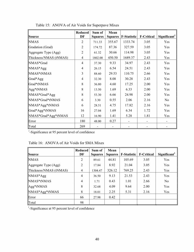
Table 15: ANOVA of Air Voids for Superpave Mixes …………………………. 40
Table 16: ANOVA of Air Voids for SMA Mixes ………………………………. 40
Table 17: Summary of Minimum t/NMAS to Provide 7.0 % Air Voids
in Laboratory ………………………………………………………..… 48
Table 18: Results of Air Voids for Limestone Superpave Mixes ………………… 50
Table 19: Results of Air Voids for Granite Superpave Mixes ………….………… 51
Table 20: ANOVA of Air Voids for Superpave Mixes …………………………. 53
v
Table 21: ANOVA of Air Voids for SMA Mixes ………………………………. 54
Table 22: Summary of Minimum t/NMAS Using Laboratory
Vibratory Compactor …………………………………………………… 60
Table 23 Thickness, t/NMAS, Air Voids and Water Absorption for Section 1…… 62
Table 24 Thickness, t/NMAS, Air Voids and Water Absorption for Section 2
Steel Wheel Roller……………………………….………….…… 66
Table 25 Thickness, t/NMAS, Air Voids and Water Absorption for Section 2
Steel/Rubber Tire Roller………………………………….………….… 66
Table 26 Thickness, t/NMAS, Air Voids and Water Absorption for Section 3
Steel Wheel Roller……………………………….………….………… 70
Table 27 Thickness, t/NMAS, Air Voids and Water Absorption for Section 3
Steel/Rubber Tire Roller………………………………….………….… 70
Table 28 Thickness, t/NMAS, Air Voids and Water Absorption for Section 4
Steel Wheel Roller……………………………….………….……….… 73
Table 29 Thickness, t/NMAS, Air Voids and Water Absorption for Section 4
Steel/Rubber Tire Roller………………………….………………..….… 74
Table 30 Thickness, t/NMAS, Air Voids and Water Absorption for Section 5
Steel Wheel Roller……………………………….………….………..… 76
Table 31 Thickness, t/NMAS, Air Voids and Water Absorption for Section 6
Steel Wheel Roller……………………………….………….………..… 79
Table 32 Thickness, t/NMAS, Air Voids and Water Absorption for Section 6
Steel/Rubber Tire Roller………………………………….………….… 79
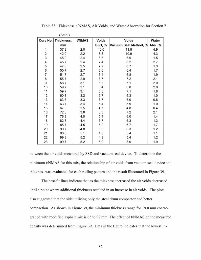
Table 33 Thickness, t/NMAS, Air Voids and Water Absorption for Section 6
vi
Steel Wheel Roller……………………………….………….………..… 82
Table 34 Thickness, t/NMAS, Air Voids and Water Absorption for Section 6
Steel/Rubber Tire Roller………………………………….………….… 83
Table 35: T/NMAS, Temperature at 20 min., Asphalt Type and Difference in
Temperature…………………………………………………………… 85
Table 36: Results of Permeability Testing Using Gyratory Compactor ………… 92
Table 37: Results of Permeability Testing Using Vibratory Compactor ………… 94
Table 38: Permeability Results for 9.5 mm Fine-Graded –Steel Roller …………. 95
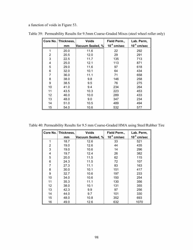
Table 39: Permeability Results for 9.5 mm Coarse-Graded –Steel Roller ………. 98
Table 40: Permeability Results for 9.5 mm Coarse-Graded –Steel/RubberTire …. 98
Table 41: Permeability Results for 9.5 mm SMA –Steel Roller ……………….…. 100
Table 42: Permeability Results for 9.5 mm SMA –Steel/RubberTire ……………. 101
Table 43: Permeability Results for 12.5 mm SMA –Steel Roller ………………….103
Table 44: Permeability Results for 12.5 mm SMA –Steel/RubberTire ………….... 104
Table 45: Permeability Results for 19.0 mm Fine-Graded –Steel Roller ………… 106
Table 46: Permeability Results for 19.0 mm Coarse-Graded –Steel Roller………. 108
Table 47: Permeability Results for 19.0 mm Coarse-Graded –Steel/Rubber Tire... 109
Table 48: Permeability Results for 19.0 mm Coarse-Graded
with Modified Asphalt –Steel Roller………………………………….... 111
Table 49: Permeability Results for 19.0 mm Coarse-Graded
With Modified Asphalt –Steel/Rubber Tire Roller……………….……. 112
Table 50: Average Air Voids, Water Absorption and Permeability
For Field Projects ……………………………………………………… 115
vii
Table 51: Best Subsets Regression on Factors Affecting Permeability …………. 120
Table 52: Effect of t/NMAS on Compactibility of HMA…………..…………… 122
viii
LIST OF FIGURES
Page
Figure 1: Experimental Plan for Part 1 of Task 3 ………………………………… 4
Figure 2: Experimental Plan for Field Study……………………………………… 7
Figure 3: Experimental Plan for Part 2 …………………………………………… 8
Figure 4: Thermocouple Location in Asphalt Mat ………………………………. 13
Figure 5: Permeability Test Conducted at Each Location ……………………….. 16
Figure 6: 9.5 mm NMAS Superpave Gradations ………………………………… 20
Figure 7: 19.0 mm NMAS Superpave Gradations ………………………………. 20
Figure 8: 37.5 mm NMAS Superpave Gradations ……………………………….. 21
Figure 9: SMA Gradations ……………………..………………………………… 21
Figure 10: Plot of 9.5 mm NMAS Gradations …………………………………… 27
Figure 11: Plot of 12.5 mm NMAS Gradations ………………………………… 28
Figure 12: Plot of 19.0 mm NMAS Gradations ………………………………… 28
Figure 13: Relationship Between Air Voids for ARZ Mixes……………………. 37
Figure 14: Relationship Between Air Voids for TRZ Mixes…………………….. 37
Figure 15: Relationship Between Air Voids for BRZ Mixes…………………….. 38
Figure 16: Relationship Between Air Voids for SMA Mixes…………………….. 38
Figure 17: Relationships of t/NMAS and Air Voids for Superpave Mixes……….. 41
Figure 18: Relationships of Gradations and Air Voids for Superpave Mixes…….. 41
Figure 19: Relationships of t/NMAS and Air Voids for SMA Mixes…………….. 42
Figure 20: Relationships Between Air Voids and t/NMAS for 9.5 mm
Superpave Mixes ……………………………………………………… 44
ix
Figure 21: Relationships Between Air Voids and t/NMAS for 19.0 mm
Superpave Mixes ……………………………………………………… 45
Figure 22: Relationships Between Air Voids and t/NMAS for 37.5 mm
Superpave Mixes ……………………………………………………… 45
Figure 23: Relationships Between Air Voids and t/NMAS for 9.5 mm
SMA Mixes …………………………………………………………… 46
Figure 24: Relationships Between Air Voids and t/NMAS for 12.5 mm
SMA Mixes …………………………………………………………… 47
Figure 25: Relationships Between Air Voids and t/NMAS for 19.0 mm
Superpave Mixes ……………………………………………………… 47
Figure 26: Relationships Between Air Voids and t/NMAS for 9.5 mm
ARZ Mixes ……………………………………………………………. 57
Figure 27: Relationships Between Air Voids and t/NMAS for 9.5 mm
BRZ Mixes …………………………………………………………….. 57
Figure 28: Relationships Between Air Voids and t/NMAS for 19.0 mm
ARZ Mixes ……………………………………………………………. 58
Figure 29: Relationships Between Air Voids and t/NMAS for 19.0 mm
BRZ Mixes …………………………………………………………… 58
Figure 30: Relationships Between Air Voids and t/NMAS for 9.5 mm
SMA Mixes ……………………………………………………………. 59
Figure 31: Relationships Between Air Voids and t/NMAS for 12.5 mm
SMA Mixes ……………………………………………………………. 59
Figure 32: Relationships Between Air Voids and t/NMAS for 19.0 mm
x
SMA Mixes ……………………………………………………………. 60
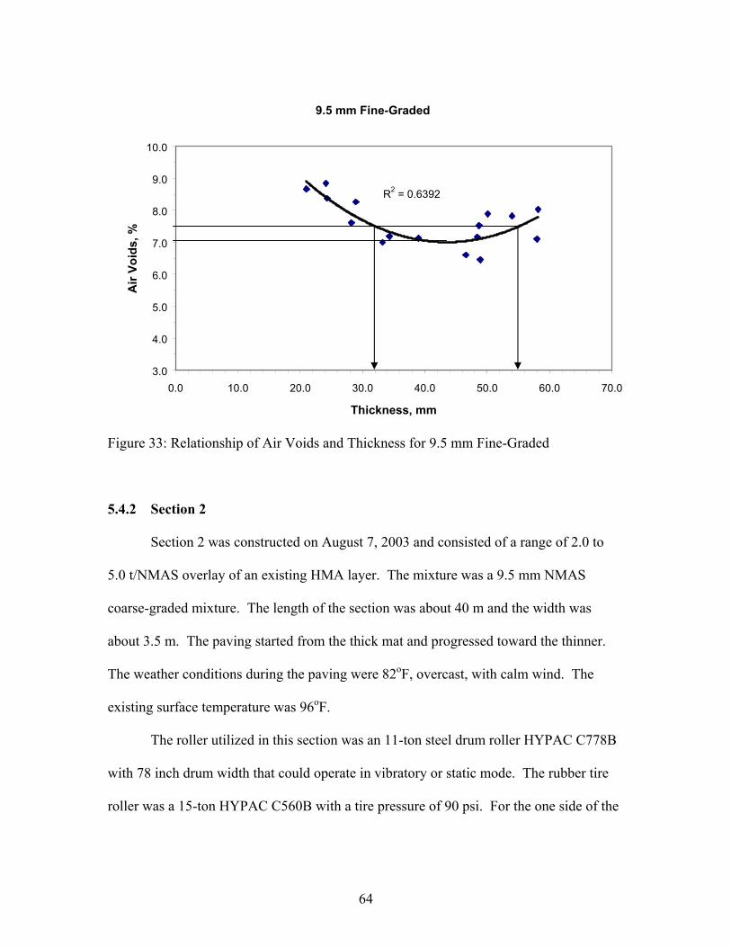
Figure 33: Relationships of Air Voids and Thickness for 9.5 mm
Fine-Graded Mix………………………………………………………. 64
Figure 34: Relationships of Air Voids and Thickness for 9.5 mm
Coarse-Graded Mix……………………………………………………. 67
Figure 35: Relationships of Air Voids and Thickness for 9.5 mm
SMA Mix……………………………………………………………. 71
Figure 36: Relationships of Air Voids and Thickness for 12.5 mm
SMA Mix………………………………………………………….…. 74
Figure 37: Relationships of Air Voids and Thickness for 19.0 mm
Fine-Graded Mix………………………………………………………. 77
Figure 38: Relationships of Air Voids and Thickness for 19.0 mm
Coarse-Graded Mix……………………………………………………. 80
Figure 39: Relationships of Air Voids and Thickness for 19.0 mm
Coarse-Graded Mix with Modified Asphalt….………………………. 84
Figure 40: Relationships Between Density, t/NMAS and Temperature for
Section 1……………………………………………………………… 86
Figure 41: Relationships Between Density, t/NMAS and Temperature for
Section 2……………………………………………………………… 86
Figure 42: Relationships Between Density, t/NMAS and Temperature for
Section 3……………………………………………………………… 87
Figure 43: Relationships Between Density, t/NMAS and Temperature for
Section 4……………………………………………………………… 87
xi
Figure 44: Relationships Between Density, t/NMAS and Temperature for
Section 5……………………………………………………………… 88
Figure 45: Relationships Between Density, t/NMAS and Temperature for
Section 6……………………………………………………………… 88
Figure 46: Relationships Between Density, t/NMAS and Temperature for
Section 7……………………………………………………………… 89
Figure 47: Relationships Between Density, and t/NMAS for All Sections…… 90
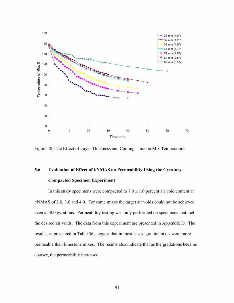
Figure 48: The Effect of Layer Thickness and Cooling Time on Mix
Temperature ………………………………………………………… 91
Figure 49: Relationships Between Permeability and t/NMAS …………………... 95
Figure 50: Permeability of 9.5 mm Fine-Graded Mix and Thickness ……………. 96
Figure 51: Permeability of 9.5 mm Fine-Graded Mix and Air Voids ……………. 97
Figure 52: Permeability of 9.5 mm Coarse-Graded Mix and Thickness …………. 99
Figure 53: Permeability of 9.5 mm Coarse-Graded Mix and Air Voids …………. 99
Figure 54: Permeability of 9.5 mm SMA Mix and Thickness ……………………. 101
Figure 55: Permeability of 9.5 mm SMA Mix and Air Voids ……………………. 102
Figure 56: Permeability of 12.5 mm SMA Mix and Thickness ……….…………. 105
Figure 57: Permeability of 9.5 mm SMA Mix and Air Voids ……………………. 105
Figure 58: Permeability of 19.0 mm Fine-Graded Mix and Thickness ………….. 107
Figure 59: Permeability of 19.0 mm Fine-Graded Mix and Air Voids ………….. 107
Figure 60: Permeability of 19.0 mm Coarse-Graded Mix and Thickness ……….. 109
Figure 61: Permeability of 19.0 mm Coarse-Graded Mix and Air Voids ..………. 110
Figure 62: Permeability of 19.0 mm Coarse-Graded Mix with
xii
Modified Asphalt and Thickness …………………………..…………. 113
Figure 63: Permeability of 19.0 mm Coarse-Graded Mix with
Modified Asphalt and Air Voids …………………………………..…. 113
Figure 64: Plot of In-place Air Voids Versus Permeability for all data …………. 116
Figure 65: Plot of In-place Air Voids Versus Permeability for 9.5 mm
NMAS Mixes …………………………………………….……………. 116
Figure 66: Plot of In-place Air Voids Versus Permeability for 12.5 mm
NMAS Mixes …………………………………………….……………. 118
Figure 67: Plot of In-place Air Voids Versus Permeability for 19.0 mm
NMAS Mixes …………………………………………….……………. 119
1
RELATIONSHIPS OF HMA IN-PLACE AIR VOIDS, LIFT THICKNESS, AND PERMEABILITY
NCHRP 9-27 Task 3 – Part 1 and 2
1.0 INTRODUCTION AND PROBLEM STATEMENT
Proper compaction of HMA mixtures is vital to ensure that a stable and durable
pavement is built. For dense-graded mixes, numerous studies have shown that initial in-
place air voids should not be below approximately 3 percent nor above approximately 8
percent (1). Low in-place air voids can result in rutting and shoving, while high air voids
allow water and air to penetrate into the pavement leading to an increased potential for
water damage, oxidation, raveling, and cracking. Low in-place air voids are generally the
result of a mix problem while high in-place voids are generally caused by inadequate
compaction.
Many researchers have shown that increases in in-place air void contents have
meant increases in pavement permeability. Zube (2) in the 1960's indicated dense-graded
pavements become excessively permeable at in-place air voids above 8 percent. Brown et
al. (3) later confirmed this value during the 1980s. However, due to problems associated
with coarse-graded (gradation passing below the maximum density line) mixes, the size
and interconnectivity of air voids have been shown to greatly influence permeability. A
study conducted by the Florida Department of Transportation (FDOT) (4) indicated that
coarse-graded Superpave mixes can be excessively permeable to water at in-place air
voids less than 8 percent. Permeability is also a major concern in stone matrix asphalt
(SMA) mixes since they utilize a gap-graded coarse gradation. Data has shown that
SMA mixes tend to become permeable when air voids are above approximately 6
percent.
2
Numerous factors can potentially affect the permeability of HMA pavements. In a
study by Ford and McWilliams (5), it was suggested that particle size distribution,
particle shape, and density (air voids or percent compaction) affect permeability. Hudson
and Davis (6) concluded that permeability is dependent on the size of air voids within a
pavement, not just the percentage of voids. Research by Mallick et al. (7) has also shown
that the nominal maximum aggregate size (NMAS) and lift thickness for a given NMAS
affect permeability.
Work by FDOT indicated that lift thickness can have an influence on density, and
hence permeability (8). FDOT constructed numerous pavement test sections on Interstate
75 that included mixes of different NMAS and lift thicknesses. Results of this experiment
suggested that increased lift thicknesses could lead to better pavement density and, hence,
lower permeability.
The three items discussed (permeability, lift thickness, and air voids) are all
interrelated. Permeability has been shown to be related to pavement density (in-place air
voids). Increased lift thickness has been shown to allow desirable density levels to be
more easily achieved. Westerman (9), Choubane et al. (4), and Musselman et al. (8) have
suggested that a thickness to NMAS ratio (t/NMAS) of 4.0 is preferred. Most guidance
recommends that a minimum t/NMAS of 3.0 be used (10). However, due to the potential
problems of achieving the desired density, it is believed that this ratio should be further
evaluated based on NMAS, gradation and mix type (Superpave and SMA).
This report is divided into 5 volumes. The first volume includes the work on Task
3-Part 1 and 2. The second volume includes the work on Task 3-Part 3. The third
volume includes the work on Task 5. The fourth volume is the appendix. The fifth
3
volume is an executive summary of the work.
2.0 OBJECTIVE
The objectives of this study are 1) to determine the minimum t/NMAS needed for
desirable pavement density levels to be achievable, and thus impermeable pavements, 2)
to evaluate the permeability characteristics of compacted samples at different thicknesses,
and 3) to evaluate factors affecting the relationship between in-place air voids,
permeability, and lift thickness.
3.0 RESEARCH APPROACH
The laboratory evaluation of the relationship between thickness, density, and
permeability was divided into two parts. Part 1 evaluated the relationship of lift
thickness, air voids, and permeability in a controlled, statistically designed experiment.
Figure 1 illustrates the research approach to evaluate these relationships. The
relationship between lift thickness and air voids is essentially one of compactability.
Enough mixture is needed on the roadway (lift thickness) so that aggregate particles can
orient themselves in such a way that a desirable density can be achieved (assuming
sufficient compactive effort). If sufficient mix is not available (lift thickness too thin),
then aggregate particles cannot slide past each other and orient in such a way as to allow
a desirable density level to be achieved. Another problem with thinner lifts is that the
mixture tends to cool more quickly, which also hinders adequate compaction. Therefore,
the objective of Part 1 was to identify the minimum thickness(es) of HMA that is needed
on the roadway to allow a desirable density to be achieved. Since lift thickness, air voids,
4
Figure 1: Experimental Plan for Part 1 of Task 3
Task 3, Part 1
Evaluate Lift Thickness vs. Air Voids (Using Vibratory Compactor)
Materials: 2 Aggregates: Limestone, Granite 3 Gradations: ARZ, BRZ, SMA 2 Superpave NMAS: 9.5, 19.0 3 SMA NMAS: 9.5, 12.5, 19.0 (Total of 14 Mixes)
3 thicknesses: 2.0, 3.0, and 4.0 t/NMAS Compact 2 replicates per combination using 3 compactive efforts: 30, 60, and 90 seconds Compact to desired height ±3 mm
Measure Gmb Using AASHTO T166 and Vacuum Sealing Method
Analyze data to determine minimum t/NMAS Based upon Gmb
Recommend Minimum Lift Thickness
Evaluate Lift Thickness vs. Air Voids (Using Gyratory Compactor)
Materials: 3 Aggregates: Limestone, Granite, Gravel 4 Gradations: ARZ, TRZ, BRZ, SMA 3 Superpave NMAS: 9.5, 19.0, 37.5 3 SMA NMAS: 9.5, 12.5, 19.0 (Total of 36 Mixes)
Mix Design
3 thicknesses: 2.0, 3.0, and 4.0 t/NMAS Compact 3 replicates per combination using standard compactive effort (N = 100 gyrations) Compact to desired height ±3 mm
Measure Gmb Using AASHTO T166 and Vacuum Sealing Method
Recommend Minimum Lift Thickness
Analyze data to determine minimum t/NMAS Based upon Gmb
Continue on next page
5
Figure 1 (cont.): Experimental Plan for Part 1
Part 1 (cont.)
Evaluate Lift Thickness vs. Permeability
Materials: 2 Aggregates: Limestone, Granite 3 Gradations: ARZ, BRZ, SMA 2 Superpave NMAS: 9.5, 19.0 3 SMA NMAS: 9.5, 12.5, 19.0 (Total of 14 Mixes)
3 thicknesses: 2.0, 3.0, and 4.0 t/NMAS
Compact 2 replicates per combination using vibratory compactor to desired void content (7 ± 1%) determined by vacuum sealing method
Measure Permeability Using ASTM PS 129-01
Analyze data to evaluate relationship between permeability and lift thickness
Make recommendation regarding the relationship
Compact 3 replicates per combination using gyratory compactor to desired void content (7 ± 1%) determined by vacuum sealing method
6
and permeability are interrelated; another objective was to investigate the permeability
characteristics of compacted HMA at different thicknesses.
After completion of the laboratory study, NCAT decided to conduct field tests to
confirm and improve on the results from the laboratory tests. This was not part of the
proposed work but it was considered necessary to better understand the effects of
thickness on compaction. The reconstruction of the 2003 NCAT Test Track gave NCAT
the opportunity to build sections (off the track) with varying thickness from one end of
each section to the other. Through the field experiments, the following issues were also
evaluated to strengthen the conclusions of this study: 1) How does lift thickness affect the
compactibility of HMA mixes, and 2) What effect does a pneumatic tire roller have on
density and permeability as compared to a steel drum roller? Figure 2 illustrates the
research approach for this part of the study.
Part 2 of this research project evaluated the relationship between in-place air
voids and laboratory permeability of core samples from NCHRP 9-9(1). Figure 3
illustrates the research approach to evaluate this relationship. Other factors influencing
the permeability such as gradation, NMAS, lift thickness, and design compactive effort
(Ndes) were also investigated.
3.1 Part 1-Experimental Plan
3.1.1 Evaluation of Effect of t/NMAS on Density Using Gyratory Compactor
In the experimental plan, a total of 36 HMA mixes were designed. Mixes were
designed having different aggregates, gradations, and NMASs. The aggregates utilized in
this research were a crushed siliceous gravel, a granite, and a limestone. These aggregates
7
Figure 2: Experimental Plan for Field Study
Analyze data to draw conclusions and make recommendations concerning the relationship between lift thickness, in-place air voids and laboratory permeability and effects of roller type on density and permeability.
Analyze data to determine minimum t/NMAS
Evaluate relationship between lift thickness, in-place air voids and permeability
Utilize seven mixes from 2003 NCAT Test Track projects with different gradation shapes, NMAS.
Construct about 40 meter long sections for each mix at increasing thickness (2.0 to 5.0 t/NMAS). One side of each paving lane utilized only a steel drum compactor and the other side incorporated a pneumatic tire roller as an intermediate roller.
Measure thickness and perform bulk specific gravity using AASHTO T 166, vacuum seal device and lab permeability for each core
Field Study
Select a minimum of 12 test locations at increasing t/NMAS and perform two field permeability tests and cut one core in between the two permeability test points for each side of mat.
8
Figure 3: Experimental Plan for Part 2
were selected because they represent a wide range of mineralogical origin, particle shape,
and surface texture. The asphalt binder utilized for all mixes was a PG 64-22. All
samples were compacted using a Superpave gyratory compactor at the temperature that
provides the recommended viscosity for the asphalt binder during the mix design.
Draw conclusions and make recommendations concerning the relationship between in-place air voids and laboratory permeability.
Perform statistical analysis to determine the statistical significance of the factors (gradation type, NMAS, thickness, and design gyrations) on the relationship between permeability and air voids.
Perform laboratory permeability using ASTM PS 129-01
Evaluate relationship between in place air voids and laboratory permeability
Utilize cores from NCHRP 9-9(1) projects with 40 mixes of different gradation shapes, NMAS, thickness, and design gyrations.
Obtain 9 cores per mix immediately after construction.
Perform bulk specific gravity using AASHTO T 166 and Vacuum seal
Part 2
9
The experiment also included four gradation shapes and three nominal maximum
aggregate sizes (NMAS). Three gradations fell within Superpave gradation control points
and one gradation conformed to stone matrix asphalt specifications. For the gradations
meeting the Superpave requirements, NMASs of 9.5, 19.0 and 37.5 mm were
investigated. For the SMA gradations, NMASs of 9.5, 12.5, and 19.0 mm were utilized.
The three Superpave gradations included one gradation that passed near the upper
gradation control limits and above the restricted zone (ARZ), one that resided near the
maximum density line and passed through the restricted zone (TRZ), and one that passed
near the lower gradation control limits and below the restricted zone (BRZ). This
resulted in a total of 36 mix designs.
The property selected to define lift thickness in this experiment was the ratio of
thickness to NMAS (t/NMAS). This ratio was selected for two reasons: (1) the ratio
normalizes lift thickness for any type of gradation and (2) a general rule-of-thumb for
Superpave mixes has been a t/NMAS ratio of 3.0 be used during construction (10). For
each NMAS in the experiment, three t/NMAS ratios were investigated. For the 9.5 and
19.0 mm NMAS Superpave mixes and all three SMA NMASs (9.5, 12.5, and 19.0 mm),
t/NMAS ratios of 2.0, 3.0, and 4.0 were used. Additional ratios of 8.0 and 6.0 for 9.5 and
12.5 mm NMAS, respectively, were also evaluated to better define the relationship where
air voids reach a limiting value (approximately 4.0 percent air voids). For the 37.5 mm
NMAS Superpave mixes, ratios of 2.0, 2.5, and 3.0 were investigated. The 4.0 t/NMAS
was excluded for the 37.5 mm NMAS mixes since this ratio would produce a 150 mm (6
in.) lift thickness which is unlikely to be used in the field. The desired thicknesses of
samples (2.0, 2.5, 3.0, 4.0, 6.0 and 8.0 t/NMAS) were achieved by altering the mass
10
placed in the mold prior to compaction (as mass changes for a given compactive effort,
thickness will change). All samples were short-term aged prior to compaction according
to “Standard Practice for Mixture Conditioning of HMA”, AASHTO PP2-01. This
procedure simulates aging of mixture during production and placement.
Three replicates of each aggregate-gradation-NMAS-thickness combination were
compacted using a single Superpave gyratory compactor. For the Superpave mixes, each
sample was compacted to 100 gyrations, the upper limit that most state DOTs use. The
100-gyration level was selected because it is probably the compactive effort that presents
the most difficulty in obtaining adequate density. For the SMA mixes, each sample was
compacted to 75 gyrations in the Superpave gyratory compactor in accordance with the
“Standard Practice for Designing SMA”, AASHTO PP44-01. The reason for using 75
gyrations was that all the aggregate types had Los Angeles abrasion values of more than
30 percent. Cellulose fiber was used as the fiber within the SMA mixes at 0.3 percent of
total mass. Designs were conducted to determine the asphalt binder content necessary to
produce 4.0 percent air voids at the design number of gyrations. Testing of each sample
after compaction included measuring the bulk specific gravity of each replicate using
both AASHTO T166 and the vacuum sealing method. A standard test method has been
developed for the vacuum sealing method, ASTM D6752-02a, “Bulk Specific Gravity
and Density of Compacted Bituminous Mixtures Using Automatic Vacuum Sealing
Method.” A statistical analysis of the data was then conducted.
3.1.2 Evaluation of Effect of t/NMAS on Density Using Vibratory Compactor
To further evaluate the relationship between density and lift thickness, a similar
11
study was conducted but on a smaller scale, using the vibratory compactor as the
compaction mode. This was not part of the original proposed work but it was believed
that the vibratory compactor might provide compaction that has more typical of in-place
compaction. Of the 36 mix designs from Part 1, 14 mixes were selected for this study.
Two types of aggregates, granite and limestone were used. For Superpave designed
mixes, two gradations were utilized (ARZ and BRZ) along with two NMASs (9.5 mm
and 19.0 mm). The 37.5 mm NMAS mix was excluded from the study because the
maximum thickness of the vibratory specimen that could be obtained was 75.0 mm,
which would only be 2.0 t/NMAS. For the SMA mixes, three NMASs were selected (9.5
mm, 12.5 mm and 19 mm). The t/NMAS ratios utilized were 2.0, 3.0 and 4.0. The
compactive effort for each t/NMAS was varied over a range including 30 sec, 60 sec, and
90 sec of compaction. The range of compactive efforts was selected for two reasons: (1)
there is no standard compactive effort for the vibratory compactor and (2) the effects of
compactive effort on density at different thicknesses could be evaluated. After
compaction, the bulk specific gravity was measured and the data was analyzed to provide
recommendations concerning the minimum t/NMAS.
3.1.3 Evaluation of Effect of t/NMAS on Density Using Field Experiment
NCAT also conducted a field study to evaluate the acceptable minimum lift
thickness. Through the field experiments, the following issues were also evaluated to
strengthen the conclusions of this study: 1) How does lift thickness affect the
compactibility of HMA mixes, and 2) What effect does a pneumatic tire roller have on
density as compared to a steel drum roller?
12
Seven mixes from the 2003 NCAT Test Track study were selected consisting of
the NMASs, gradations, and mix types (Superpave and SMA) shown in Table 1.
Table 1: Mix Information for Field Density Study
Section NMAS Gradation Asphalt Type Aggregate Type 1 9.5 mm Fine-Graded
Superpave Unmodified Granite and
Limestone 2 9.5 mm Coarse-Graded
Superpave Unmodified Limestone
3 9.5 mm SMA Modified Granite 4 12.5 mm SMA Modified Limestone 5 19.0 mm Fine-Graded
Superpave Unmodified Granite and
Limestone 6 19.0 mm Coarse-Graded
Superpave Unmodified Granite
7 19.0 mm Coarse-Graded Superpave
Modified Limestone
The experiment was conducted during the trial mixing stage and included the
construction of each section with t/NMAS ratios ranging from approximately 2.0 to 5.0
on the seven sections at the NCAT track facilities. The desired mat thicknesses were
achieved by gradually adjusting the screed depth crank of the paver during the laydown
operation. To investigate the effect of lift thickness on the rate of cooling in the mat and
to ensure the mat was being compacted within the time available for compaction, three
locations were selected for temperature measurements for each section; one at the
beginning of the section, one at the middle and one at the end of the section. At each
location, two thermocouples were placed in the mat immediately after placement and
prior to compaction as shown in Figure 4. Surface temperatures were also obtained with
an infrared temperature gun. Temperature readings were monitored and recorded every
13
few minutes and after every roller pass. The air and base temperatures at time of
placement, as well as the weather conditions, were also recorded.
Figure 4: Thermocouple Location in Asphalt Mat
Reasonable and consistent compactive effort was applied throughout the section
regardless of the t/NMAS. To study the effect of roller type on density, one side of the
mat utilized only a steel drum compactor and the other side incorporated a pneumatic tire
roller as an intermediate roller. The steel drum roller operated in both vibratory and static
modes. A non-destructive density gauge (Pavement Quality Indicator (PQI)) was used to
monitor the density after each pass with the rollers and to determine the rate of
densification for the various thicknesses.
A minimum of twelve test locations (at increasing t/NMAS) per compactive effort
(steel wheel or pneumatic tire) was selected for testing. At each test location, one field
core was obtained approximately 2 ft from the pavement edge. This equated to a total of
at least 12 cores for each compactive effort and a total of at least 24 cores for one section
(when both roller types were used). The cores obtained were used to determine in-place
density, and thickness.
Height,HT
1 ft.Pavement Edge
Thermocouple 1
Thermocouple 2
1/3HT
2/3HT
14
3.1.4 Evaluation of Effect of Temperature on Relationship Between Density and
t/NMAS from Field Experiment
Recall from the field experiment that three locations were selected for
temperature measurements for each section; one near the beginning of the section, one
near the middle, and one near the end of section. This was done because the rate of
cooling varied from one end to the other due to change of thickness. The rate of cooling
was determined by plotting the average temperature from each location against time. To
determine the effect of temperature on the density, the temperature at 20 minutes after
placement of mix was selected. This number is somewhat arbitrary but it is realistic
because in general, the compaction in the field should be obtained within approximately
20 minutes after paving. Since the mixes in this study used two different types of asphalt
binder, (PG 67-22 and PG 76-22), the temperatures at 20 minutes were normalized by
subtracting the high temperature grade of the asphalt binder from the measured mat
temperatures at 20 minutes. For instance, if the temperature at 20 minutes was 100oC for
a mix using PG 67-22, the difference of the temperature was 33oC (100oC – 67oC). This
was done because in general the higher PG binder (PG 76-22) would require a higher
compaction temperature and hence it is the difference in the mix temperature and the high
temperature PG grade that affects compaction.
3.1.5 Evaluation of Effect of t/NMAS on Permeability Using Gyratory Compactor
To investigate the permeability characteristics of HMA at different thicknesses,
the same 14 mixes used in the experiment to determine the effect of t/NMAS on density
using vibratory compactor were utilized. The gyratory compactor height for t/NMAS
15
ratios of 2.0, 3.0, and 4.0 was determined and samples were compacted with appropriate
mass to produce 7.0 ± 1 percent air voids. The 7.0 percent air voids was selected to
simulate the density of a pavement in the field after construction. The bulk specific
gravity was measured using the vacuum seal method. Permeability tests were performed
on all samples and the relationships between permeability and lift thickness evaluated.
3.1.6 Evaluation of Effect of t/NMAS on Permeability Using Vibratory Compactor
For this study, the same 14 mixes used in the previous vibratory compactor study
were utilized. T/NMAS ratios of 2.0, 3.0, and 4.0 were used and two beams of each
aggregate-gradation-t/NMAS combination were compacted to 7.0 ± 1 percent air voids.
Two 100 mm cores were cut from the beams. Bulk specific gravity for beams and cores
was determined using the vacuum seal method. Permeability tests were performed on all
core samples and the relationships between permeability and lift thickness evaluated.
3.1.7 Evaluation of the Effect of t/NMAS on Permeability Using Field Experiment
The seven sections constructed to determine the minimum t/NMAS from the field
experiment were utilized in this study. The effect of roller type on permeability was also
evaluated. A minimum of twelve test locations per compactive effort (steel wheel or
pneumatic tire) was selected for testing. Two field permeability tests were performed at
the locations where the cores were obtained as shown in Figure 5. Laboratory
permeability testing was also performed on the cores obtained from each section. This
was done to evaluate the relationships between laboratory and field permeability tests.
16
Field Permeability Test
Core
Figure 5: Testing Conducted at Each Test Location.
3.2 Part 2 Experimental Plan – Evaluation of Relationship of Laboratory
Permeability, In-place Air Voids, and Lift Thickness of Field Compacted
Cores (NCHRP 9-9(1))
Part 2 evaluated the relationship between in-place air voids and laboratory
permeability. Figure 2 illustrates the research approach to evaluate this relationship. A
total of 40 on-going HMA construction projects were visited by NCAT during NCHRP
9-9(1) “Verification of Gyration Levels in the Ndes Table”. Five different combinations
of gradation shape and NMAS were studied: fine-graded 9.5 mm, 12.5 mm, and 19.0 mm
NMAS mixes and coarse-graded 9.5 mm and 12.5 mm NMAS mixes. At each of the
projects, cores were obtained from the roadway after construction but before traffic so
that the actual lift thickness and in-place air voids could be determined. Cores brought
back to the laboratory from NCHRP 9-9(1) field projects were sawed and tested for bulk
specific gravity (AASHTO T 166 and the vacuum seal methods), thickness, and
Direction of Travel
25.4 cm
25.4 cm
25.4 cm
17
laboratory permeability (ASTM PS 129-01). Plant-produced mix was also sampled at
each project in order to determine the theoretical maximum density (TMD) and the
mixture gradation. The TMD test was performed according to AASHTO T209.
4.0 MATERIALS AND TEST METHODS
4.1 Aggregate and Binder Properties
Properties of the coarse and fine aggregates utilized in the laboratory experiments
of Part 1 study are shown in Table 2. The aggregates were selected to represent a range
of physical properties, such as bulk specific gravity (2.585 to 2.725), flat and elongated
particles (4 to 14 percent at 3:1), Los Angeles abrasion (31 to 37 percent), coarse
aggregate angularity (42.9 to 44.0 percent), and fine aggregate angularity (45.7 to 49.4
percent). This variability in aggregate properties, while not very different, should
provide some variability of mix properties.
Table 3 presents the test results for the asphalt binder utilized in the study. The
binder was classified as PG 64-22 and is commonly used for warm to moderate climates.
The binder met high temperature property criteria at a temperature of 67oC and so can be
classified as a PG 67-22.
18
Table 2: Physical Properties of Aggregate
Aggregate Type Property Test Method
Granite Limestone Crushed Gravel
Coarse Aggregate
Bulk Specific Gravity AASHTO T-85 2.654 2.725 2.585
Apparent Specific Gravity AASHTO T-85 2.704 2.758 2.642
Absorption (%) AASHTO T-85 0.7 0.4 0.9
19.0 mm 14, 0 10, 0 4, 0
12.5 mm 16, 0 6, 0 16, 2 Flat and
Elongated (%), 3:1, 5:1 9.0 mm
ASTM D4791
9, 1 16, 3 19, 2
Los Angeles Abrasion (%) AASHTO T-96 37 35 31 Coarse Aggregate
Angularity (%) AASHTO TP56-99 42.9 43.0 44.0
Percent Crushed (%) ASTM D5821 100 100 80
Fine Aggregate
Bulk Specific Gravity AASHTO T-84 2.678 2.689 2.610
Apparent Specific Gravity AASHTO T-84 2.700 2.752 2.645
Ln (CL) = natural log of air voids from vacuum sealed device
CAratio = coarse aggregate ratio
Ln(VMA) = natural log of voids in mineral aggregate
Table 51: Best Subsets Regression on Factors Affecting Permeability No. of
Variables R-Sq R-Sq(adj) C-p NMAS Thickness Ln (CL) CAratio Ln (VMA)1 68.5 68.4 31.3 X 1 43.2 42.9 235.1 X 2 71.6 71.4 8.2 X X 2 70.2 69.9 19.8 X X 3 72.5 72.2 3.1 X X X 3 71.8 71.5 8.5 X X X 4 72.6 72.1 4.1 X X X X 4 72.5 72 4.9 X X X X 5 72.7 72 6 X X X X X
121
There was a good correlation for the above equation with an R2 of 0.72. The
equation indicated that permeability increased as the air voids increased. The
illustrations of this relationship are presented in the previous figures. The permeability
also increased as the coarse aggregate ratio increased. The coarser the gradations, the
larger the individual air voids leading to higher potential for interconnected air voids.
The equation also suggested that the permeability increased as the VMA decreased.
Lower VMA suggests less room for asphalt cement in a mix, which results in higher
potential for interconnected air voids.
6.0 DISCUSSION OF RESULTS
6.1 Determination of the Minimum t/NMAS
The minimum t/NMAS determined from both gyratory and vibratory compactors
was discussed earlier. Neither of these methods appeared to provide a clear approach for
selecting the minimum t/NMAS. The results that provided the clearest answer to the
minimum t/NMAS were obtained from the HMA sections constructed at the NCAT test
track. For these sections the thickness was varied from relatively thin to relatively thick
and a reasonable compactive effort with conventional rollers was applied. The results
from these 7 mixtures appeared to provide suitable numbers that could be used to provide
guidance on selecting minimum t/NMAS ratios. The data determined from this part of
the study are summarized and presented in Table 52.
The results shown in Table 52 indicate that t/NMAS clearly has an effect on the
compactibility of HMA mixes. This table shows the effect of changing the t/NMAS.
The numbers presented indicate the difference between the air voids at the t/NMAS
indicated and the lowest air voids at optimum t/NMAS.
122
Table 52: Effect of t/NMAS on Compactibility of HMA
Description of Mix
Difference from Minimum Air Voids for t/NMAS=2
Difference from Minimum Air Voids for t/NMAS=3
Difference from Minimum Air Voids for t/NMAS=4
Difference from Minimum Air Voids for t/NMAS=5
Section 1-9.5mm Fine Graded—Steel Roller
2.5% 1.0% 0.1% 0.1%
Section 2-9.5mm Coarse Graded-Steel Roller
2.5% 1.0% 0.5% 0.0%
Section 2-9.5mm Coarse Graded-Steel and Rubber Roller
2.0% 0.5% 0.0% 1.0%
Section 3-9.5mm SMA(mod AC) Steel Roller
5.5% 2.0% 0.2% 0.2%
Section 3-9.5mm SMA(Mod AC) Steel & Rubber Roller
1.2% 0.2% 0.0% 0.5%
Section 4-12.5mm SMA (mod AC) Steel Roller
11.3% 3.3% 0.3% 0.5%
Section 4-12.5mm SMA (mod AC) Steel & Rubber Roller
6.5% 3.5% 0.5% 0.0%
Section 5-19mm Fine Graded Steel Roller
3.1% 0.6% 0.0% 1.3%
Section 6-19mm Coarse Graded Steel and Rubber Roller