462
Robotics Toolbox for MATLAB ® Release 10 Peter Corke
Robotics Toolboxfor MATLAB®
Release 10
Peter Corke
2
Release 10.4Release date September 2020
Licence LGPLToolbox home page http://www.petercorke.com/robotDiscussion group http://groups.google.com.au/group/robotics-tool-box
Copyright ©2020Peter [email protected]://www.petercorke.com
Preface
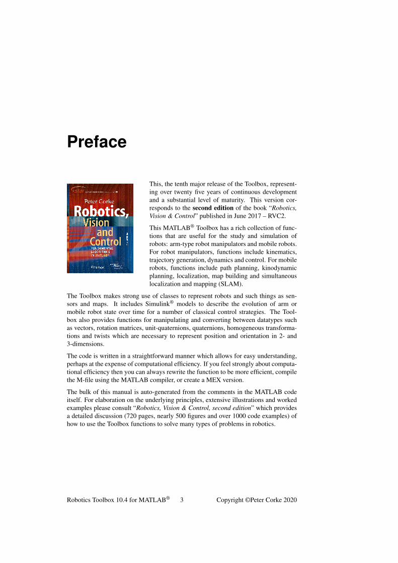
This, the tenth major release of the Toolbox, represent-ing over twenty five years of continuous developmentand a substantial level of maturity. This version cor-responds to the second edition of the book “Robotics,Vision & Control” published in June 2017 – RVC2.
This MATLAB® Toolbox has a rich collection of func-tions that are useful for the study and simulation ofrobots: arm-type robot manipulators and mobile robots.For robot manipulators, functions include kinematics,trajectory generation, dynamics and control. For mobilerobots, functions include path planning, kinodynamicplanning, localization, map building and simultaneouslocalization and mapping (SLAM).
The Toolbox makes strong use of classes to represent robots and such things as sen-sors and maps. It includes Simulink® models to describe the evolution of arm ormobile robot state over time for a number of classical control strategies. The Tool-box also provides functions for manipulating and converting between datatypes suchas vectors, rotation matrices, unit-quaternions, quaternions, homogeneous transforma-tions and twists which are necessary to represent position and orientation in 2- and3-dimensions.
The code is written in a straightforward manner which allows for easy understanding,perhaps at the expense of computational efficiency. If you feel strongly about computa-tional efficiency then you can always rewrite the function to be more efficient, compilethe M-file using the MATLAB compiler, or create a MEX version.
The bulk of this manual is auto-generated from the comments in the MATLAB codeitself. For elaboration on the underlying principles, extensive illustrations and workedexamples please consult “Robotics, Vision & Control, second edition” which providesa detailed discussion (720 pages, nearly 500 figures and over 1000 code examples) ofhow to use the Toolbox functions to solve many types of problems in robotics.
Robotics Toolbox 10.4 for MATLAB® 3 Copyright ©Peter Corke 2020

Robotics Toolbox 10.4 for MATLAB® 4 Copyright ©Peter Corke 2020

Functions by category
Robotics Toolbox 10.4 for MATLAB® 5 Copyright ©Peter Corke 2020

Robotics Toolbox 10.4 for MATLAB® 6 Copyright ©Peter Corke 2020
Contents
Preface . . . . . . . . . . . . . . . . . . . . . . . . . . . . . . . . . . . . . 2Functions by category . . . . . . . . . . . . . . . . . . . . . . . . . . . . . 5
1 Introduction 131.1 Changes in RTB 10 . . . . . . . . . . . . . . . . . . . . . . . . . . . 13
1.1.1 Incompatible changes . . . . . . . . . . . . . . . . . . . . . . 131.1.2 New features . . . . . . . . . . . . . . . . . . . . . . . . . . 141.1.3 Enhancements . . . . . . . . . . . . . . . . . . . . . . . . . 15
1.2 Changes in RTB 10.3 . . . . . . . . . . . . . . . . . . . . . . . . . . 171.3 Changes in RTB 10.2 . . . . . . . . . . . . . . . . . . . . . . . . . . 191.4 How to obtain the Toolbox . . . . . . . . . . . . . . . . . . . . . . . 19
1.4.1 From .mltbx file . . . . . . . . . . . . . . . . . . . . . . . . 191.4.2 From .zip file . . . . . . . . . . . . . . . . . . . . . . . . . . 201.4.3 MATLAB OnlineTM . . . . . . . . . . . . . . . . . . . . . . 201.4.4 Simulink® . . . . . . . . . . . . . . . . . . . . . . . . . . . 211.4.5 Notes on implementation and versions . . . . . . . . . . . . . 241.4.6 Documentation . . . . . . . . . . . . . . . . . . . . . . . . . 24
1.5 Compatible MATLAB versions . . . . . . . . . . . . . . . . . . . . . 251.6 Use in teaching . . . . . . . . . . . . . . . . . . . . . . . . . . . . . 251.7 Use in research . . . . . . . . . . . . . . . . . . . . . . . . . . . . . 251.8 Support . . . . . . . . . . . . . . . . . . . . . . . . . . . . . . . . . 251.9 Related software . . . . . . . . . . . . . . . . . . . . . . . . . . . . 26
1.9.1 Robotics System ToolboxTM . . . . . . . . . . . . . . . . . . 261.9.2 Octave . . . . . . . . . . . . . . . . . . . . . . . . . . . . . 261.9.3 Machine Vision toolbox . . . . . . . . . . . . . . . . . . . . 26
1.10 Contributing to the Toolboxes . . . . . . . . . . . . . . . . . . . . . 271.11 Acknowledgements . . . . . . . . . . . . . . . . . . . . . . . . . . . 27
2 Functions and classes 29Astar . . . . . . . . . . . . . . . . . . . . . . . . . . . . . . . . . . . . . . 29AstarMOO . . . . . . . . . . . . . . . . . . . . . . . . . . . . . . . . . . . 35AstarPO . . . . . . . . . . . . . . . . . . . . . . . . . . . . . . . . . . . . 41Bicycle . . . . . . . . . . . . . . . . . . . . . . . . . . . . . . . . . . . . 47Bug2 . . . . . . . . . . . . . . . . . . . . . . . . . . . . . . . . . . . . . . 51ccodefunctionstring . . . . . . . . . . . . . . . . . . . . . . . . . . . . . . 53chi2inv_rtb . . . . . . . . . . . . . . . . . . . . . . . . . . . . . . . . . . 55ctraj . . . . . . . . . . . . . . . . . . . . . . . . . . . . . . . . . . . . . . 55delta2tr . . . . . . . . . . . . . . . . . . . . . . . . . . . . . . . . . . . . 56
Robotics Toolbox 10.4 for MATLAB® 7 Copyright ©Peter Corke 2020
CONTENTS CONTENTS
DHFactor . . . . . . . . . . . . . . . . . . . . . . . . . . . . . . . . . . . 56distancexform . . . . . . . . . . . . . . . . . . . . . . . . . . . . . . . . . 58distributeblocks . . . . . . . . . . . . . . . . . . . . . . . . . . . . . . . . 59doesblockexist . . . . . . . . . . . . . . . . . . . . . . . . . . . . . . . . . 59Dstar . . . . . . . . . . . . . . . . . . . . . . . . . . . . . . . . . . . . . . 60DstarMOO . . . . . . . . . . . . . . . . . . . . . . . . . . . . . . . . . . . 64DstarPO . . . . . . . . . . . . . . . . . . . . . . . . . . . . . . . . . . . . 70Dubbins . . . . . . . . . . . . . . . . . . . . . . . . . . . . . . . . . . . . 77DXform . . . . . . . . . . . . . . . . . . . . . . . . . . . . . . . . . . . . 78EKF . . . . . . . . . . . . . . . . . . . . . . . . . . . . . . . . . . . . . . 82ETS . . . . . . . . . . . . . . . . . . . . . . . . . . . . . . . . . . . . . . 90ETS2 . . . . . . . . . . . . . . . . . . . . . . . . . . . . . . . . . . . . . 92ETS3 . . . . . . . . . . . . . . . . . . . . . . . . . . . . . . . . . . . . . 101Frame . . . . . . . . . . . . . . . . . . . . . . . . . . . . . . . . . . . . . 110getprofilefunctionstats . . . . . . . . . . . . . . . . . . . . . . . . . . . . . 112joy2tr . . . . . . . . . . . . . . . . . . . . . . . . . . . . . . . . . . . . . 113joystick . . . . . . . . . . . . . . . . . . . . . . . . . . . . . . . . . . . . 113jsingu . . . . . . . . . . . . . . . . . . . . . . . . . . . . . . . . . . . . . 114jtraj . . . . . . . . . . . . . . . . . . . . . . . . . . . . . . . . . . . . . . 114LandmarkMap . . . . . . . . . . . . . . . . . . . . . . . . . . . . . . . . . 115Lattice . . . . . . . . . . . . . . . . . . . . . . . . . . . . . . . . . . . . . 118bresenham . . . . . . . . . . . . . . . . . . . . . . . . . . . . . . . . . . . 121circle . . . . . . . . . . . . . . . . . . . . . . . . . . . . . . . . . . . . . . 121colorname . . . . . . . . . . . . . . . . . . . . . . . . . . . . . . . . . . . 122diff2 . . . . . . . . . . . . . . . . . . . . . . . . . . . . . . . . . . . . . . 123dockfigs . . . . . . . . . . . . . . . . . . . . . . . . . . . . . . . . . . . . 123edgelist . . . . . . . . . . . . . . . . . . . . . . . . . . . . . . . . . . . . 123filt1d . . . . . . . . . . . . . . . . . . . . . . . . . . . . . . . . . . . . . . 124gaussfunc . . . . . . . . . . . . . . . . . . . . . . . . . . . . . . . . . . . 125mmlabel . . . . . . . . . . . . . . . . . . . . . . . . . . . . . . . . . . . . 125mplot . . . . . . . . . . . . . . . . . . . . . . . . . . . . . . . . . . . . . 126mtools . . . . . . . . . . . . . . . . . . . . . . . . . . . . . . . . . . . . . 127pickregion . . . . . . . . . . . . . . . . . . . . . . . . . . . . . . . . . . . 127plotp . . . . . . . . . . . . . . . . . . . . . . . . . . . . . . . . . . . . . . 128polydiff . . . . . . . . . . . . . . . . . . . . . . . . . . . . . . . . . . . . 128Polygon . . . . . . . . . . . . . . . . . . . . . . . . . . . . . . . . . . . . 128randinit . . . . . . . . . . . . . . . . . . . . . . . . . . . . . . . . . . . . 135runscript . . . . . . . . . . . . . . . . . . . . . . . . . . . . . . . . . . . . 135rvcpath . . . . . . . . . . . . . . . . . . . . . . . . . . . . . . . . . . . . . 136stlRead . . . . . . . . . . . . . . . . . . . . . . . . . . . . . . . . . . . . 136usefig . . . . . . . . . . . . . . . . . . . . . . . . . . . . . . . . . . . . . 137xaxis . . . . . . . . . . . . . . . . . . . . . . . . . . . . . . . . . . . . . . 137yaxis . . . . . . . . . . . . . . . . . . . . . . . . . . . . . . . . . . . . . . 138about . . . . . . . . . . . . . . . . . . . . . . . . . . . . . . . . . . . . . . 138angdiff . . . . . . . . . . . . . . . . . . . . . . . . . . . . . . . . . . . . . 139angvec2r . . . . . . . . . . . . . . . . . . . . . . . . . . . . . . . . . . . . 139angvec2tr . . . . . . . . . . . . . . . . . . . . . . . . . . . . . . . . . . . 140Animate . . . . . . . . . . . . . . . . . . . . . . . . . . . . . . . . . . . . 140circle . . . . . . . . . . . . . . . . . . . . . . . . . . . . . . . . . . . . . . 143colnorm . . . . . . . . . . . . . . . . . . . . . . . . . . . . . . . . . . . . 143
Robotics Toolbox 10.4 for MATLAB® 8 Copyright ©Peter Corke 2020
CONTENTS CONTENTS
delta2tr . . . . . . . . . . . . . . . . . . . . . . . . . . . . . . . . . . . . 144e2h . . . . . . . . . . . . . . . . . . . . . . . . . . . . . . . . . . . . . . . 144eul2jac . . . . . . . . . . . . . . . . . . . . . . . . . . . . . . . . . . . . . 145eul2r . . . . . . . . . . . . . . . . . . . . . . . . . . . . . . . . . . . . . . 145eul2tr . . . . . . . . . . . . . . . . . . . . . . . . . . . . . . . . . . . . . 146h2e . . . . . . . . . . . . . . . . . . . . . . . . . . . . . . . . . . . . . . . 147homline . . . . . . . . . . . . . . . . . . . . . . . . . . . . . . . . . . . . 147homtrans . . . . . . . . . . . . . . . . . . . . . . . . . . . . . . . . . . . . 147ishomog . . . . . . . . . . . . . . . . . . . . . . . . . . . . . . . . . . . . 148ishomog2 . . . . . . . . . . . . . . . . . . . . . . . . . . . . . . . . . . . 149isrot . . . . . . . . . . . . . . . . . . . . . . . . . . . . . . . . . . . . . . 149isrot2 . . . . . . . . . . . . . . . . . . . . . . . . . . . . . . . . . . . . . 150isunit . . . . . . . . . . . . . . . . . . . . . . . . . . . . . . . . . . . . . . 150isvec . . . . . . . . . . . . . . . . . . . . . . . . . . . . . . . . . . . . . . 151lift23 . . . . . . . . . . . . . . . . . . . . . . . . . . . . . . . . . . . . . . 151numcols . . . . . . . . . . . . . . . . . . . . . . . . . . . . . . . . . . . . 152numrows . . . . . . . . . . . . . . . . . . . . . . . . . . . . . . . . . . . . 152oa2r . . . . . . . . . . . . . . . . . . . . . . . . . . . . . . . . . . . . . . 152oa2tr . . . . . . . . . . . . . . . . . . . . . . . . . . . . . . . . . . . . . . 153PGraph . . . . . . . . . . . . . . . . . . . . . . . . . . . . . . . . . . . . 154plot2 . . . . . . . . . . . . . . . . . . . . . . . . . . . . . . . . . . . . . . 172plot_arrow . . . . . . . . . . . . . . . . . . . . . . . . . . . . . . . . . . . 173plot_box . . . . . . . . . . . . . . . . . . . . . . . . . . . . . . . . . . . . 173plot_circle . . . . . . . . . . . . . . . . . . . . . . . . . . . . . . . . . . . 175plot_ellipse . . . . . . . . . . . . . . . . . . . . . . . . . . . . . . . . . . 176plot_homline . . . . . . . . . . . . . . . . . . . . . . . . . . . . . . . . . 177plot_point . . . . . . . . . . . . . . . . . . . . . . . . . . . . . . . . . . . 178plot_poly . . . . . . . . . . . . . . . . . . . . . . . . . . . . . . . . . . . 179plot_ribbon . . . . . . . . . . . . . . . . . . . . . . . . . . . . . . . . . . 180plot_sphere . . . . . . . . . . . . . . . . . . . . . . . . . . . . . . . . . . 181plotvol . . . . . . . . . . . . . . . . . . . . . . . . . . . . . . . . . . . . . 182Plucker . . . . . . . . . . . . . . . . . . . . . . . . . . . . . . . . . . . . 182Quaternion . . . . . . . . . . . . . . . . . . . . . . . . . . . . . . . . . . . 192r2t . . . . . . . . . . . . . . . . . . . . . . . . . . . . . . . . . . . . . . . 204randinit . . . . . . . . . . . . . . . . . . . . . . . . . . . . . . . . . . . . 204rot2 . . . . . . . . . . . . . . . . . . . . . . . . . . . . . . . . . . . . . . 205rotx . . . . . . . . . . . . . . . . . . . . . . . . . . . . . . . . . . . . . . 205roty . . . . . . . . . . . . . . . . . . . . . . . . . . . . . . . . . . . . . . 206rotz . . . . . . . . . . . . . . . . . . . . . . . . . . . . . . . . . . . . . . 206rpy2jac . . . . . . . . . . . . . . . . . . . . . . . . . . . . . . . . . . . . . 206rpy2r . . . . . . . . . . . . . . . . . . . . . . . . . . . . . . . . . . . . . . 207rpy2tr . . . . . . . . . . . . . . . . . . . . . . . . . . . . . . . . . . . . . 208rt2tr . . . . . . . . . . . . . . . . . . . . . . . . . . . . . . . . . . . . . . 209RTBPose . . . . . . . . . . . . . . . . . . . . . . . . . . . . . . . . . . . 210SE2 . . . . . . . . . . . . . . . . . . . . . . . . . . . . . . . . . . . . . . 223SE3 . . . . . . . . . . . . . . . . . . . . . . . . . . . . . . . . . . . . . . 232skew . . . . . . . . . . . . . . . . . . . . . . . . . . . . . . . . . . . . . . 251skewa . . . . . . . . . . . . . . . . . . . . . . . . . . . . . . . . . . . . . 252SO2 . . . . . . . . . . . . . . . . . . . . . . . . . . . . . . . . . . . . . . 253SO3 . . . . . . . . . . . . . . . . . . . . . . . . . . . . . . . . . . . . . . 261
Robotics Toolbox 10.4 for MATLAB® 9 Copyright ©Peter Corke 2020
CONTENTS CONTENTS
SpatialAcceleration . . . . . . . . . . . . . . . . . . . . . . . . . . . . . . 278SpatialF6 . . . . . . . . . . . . . . . . . . . . . . . . . . . . . . . . . . . 280SpatialForce . . . . . . . . . . . . . . . . . . . . . . . . . . . . . . . . . . 281SpatialInertia . . . . . . . . . . . . . . . . . . . . . . . . . . . . . . . . . 282SpatialM6 . . . . . . . . . . . . . . . . . . . . . . . . . . . . . . . . . . . 285SpatialMomentum . . . . . . . . . . . . . . . . . . . . . . . . . . . . . . . 287SpatialVec6 . . . . . . . . . . . . . . . . . . . . . . . . . . . . . . . . . . 288SpatialVelocity . . . . . . . . . . . . . . . . . . . . . . . . . . . . . . . . 292stlRead . . . . . . . . . . . . . . . . . . . . . . . . . . . . . . . . . . . . 293t2r . . . . . . . . . . . . . . . . . . . . . . . . . . . . . . . . . . . . . . . 294tb_optparse . . . . . . . . . . . . . . . . . . . . . . . . . . . . . . . . . . 294tr2angvec . . . . . . . . . . . . . . . . . . . . . . . . . . . . . . . . . . . 296tr2delta . . . . . . . . . . . . . . . . . . . . . . . . . . . . . . . . . . . . 297tr2eul . . . . . . . . . . . . . . . . . . . . . . . . . . . . . . . . . . . . . 298tr2jac . . . . . . . . . . . . . . . . . . . . . . . . . . . . . . . . . . . . . 298tr2rpy . . . . . . . . . . . . . . . . . . . . . . . . . . . . . . . . . . . . . 299tr2rt . . . . . . . . . . . . . . . . . . . . . . . . . . . . . . . . . . . . . . 300tranimate . . . . . . . . . . . . . . . . . . . . . . . . . . . . . . . . . . . 300tranimate2 . . . . . . . . . . . . . . . . . . . . . . . . . . . . . . . . . . . 301transl . . . . . . . . . . . . . . . . . . . . . . . . . . . . . . . . . . . . . . 302transl2 . . . . . . . . . . . . . . . . . . . . . . . . . . . . . . . . . . . . . 303trchain . . . . . . . . . . . . . . . . . . . . . . . . . . . . . . . . . . . . . 304trchain2 . . . . . . . . . . . . . . . . . . . . . . . . . . . . . . . . . . . . 305trexp . . . . . . . . . . . . . . . . . . . . . . . . . . . . . . . . . . . . . . 306trexp2 . . . . . . . . . . . . . . . . . . . . . . . . . . . . . . . . . . . . . 307trinterp . . . . . . . . . . . . . . . . . . . . . . . . . . . . . . . . . . . . . 308trinterp2 . . . . . . . . . . . . . . . . . . . . . . . . . . . . . . . . . . . . 309trlog . . . . . . . . . . . . . . . . . . . . . . . . . . . . . . . . . . . . . . 310trnorm . . . . . . . . . . . . . . . . . . . . . . . . . . . . . . . . . . . . . 311trot2 . . . . . . . . . . . . . . . . . . . . . . . . . . . . . . . . . . . . . . 311trotx . . . . . . . . . . . . . . . . . . . . . . . . . . . . . . . . . . . . . . 312troty . . . . . . . . . . . . . . . . . . . . . . . . . . . . . . . . . . . . . . 312trotz . . . . . . . . . . . . . . . . . . . . . . . . . . . . . . . . . . . . . . 313trplot . . . . . . . . . . . . . . . . . . . . . . . . . . . . . . . . . . . . . . 313trplot2 . . . . . . . . . . . . . . . . . . . . . . . . . . . . . . . . . . . . . 315trprint . . . . . . . . . . . . . . . . . . . . . . . . . . . . . . . . . . . . . 316trprint2 . . . . . . . . . . . . . . . . . . . . . . . . . . . . . . . . . . . . 317trscale . . . . . . . . . . . . . . . . . . . . . . . . . . . . . . . . . . . . . 317Twist . . . . . . . . . . . . . . . . . . . . . . . . . . . . . . . . . . . . . . 318unit . . . . . . . . . . . . . . . . . . . . . . . . . . . . . . . . . . . . . . 324UnitQuaternion . . . . . . . . . . . . . . . . . . . . . . . . . . . . . . . . 325vex . . . . . . . . . . . . . . . . . . . . . . . . . . . . . . . . . . . . . . . 347vexa . . . . . . . . . . . . . . . . . . . . . . . . . . . . . . . . . . . . . . 348xyzlabel . . . . . . . . . . . . . . . . . . . . . . . . . . . . . . . . . . . . 349Link . . . . . . . . . . . . . . . . . . . . . . . . . . . . . . . . . . . . . . 349lspb . . . . . . . . . . . . . . . . . . . . . . . . . . . . . . . . . . . . . . 360makemap . . . . . . . . . . . . . . . . . . . . . . . . . . . . . . . . . . . 361models . . . . . . . . . . . . . . . . . . . . . . . . . . . . . . . . . . . . . 362mdl_ball . . . . . . . . . . . . . . . . . . . . . . . . . . . . . . . . . . . . 362mdl_baxter . . . . . . . . . . . . . . . . . . . . . . . . . . . . . . . . . . 363
Robotics Toolbox 10.4 for MATLAB® 10 Copyright ©Peter Corke 2020
CONTENTS CONTENTS
mdl_cobra600 . . . . . . . . . . . . . . . . . . . . . . . . . . . . . . . . . 364mdl_coil . . . . . . . . . . . . . . . . . . . . . . . . . . . . . . . . . . . . 364mdl_fanuc10L . . . . . . . . . . . . . . . . . . . . . . . . . . . . . . . . . 365mdl_hyper2d . . . . . . . . . . . . . . . . . . . . . . . . . . . . . . . . . 366mdl_hyper3d . . . . . . . . . . . . . . . . . . . . . . . . . . . . . . . . . 366mdl_irb140 . . . . . . . . . . . . . . . . . . . . . . . . . . . . . . . . . . 367mdl_irb140_mdh . . . . . . . . . . . . . . . . . . . . . . . . . . . . . . . 368mdl_jaco . . . . . . . . . . . . . . . . . . . . . . . . . . . . . . . . . . . . 369mdl_KR5 . . . . . . . . . . . . . . . . . . . . . . . . . . . . . . . . . . . 370mdl_LWR . . . . . . . . . . . . . . . . . . . . . . . . . . . . . . . . . . . 370mdl_M16 . . . . . . . . . . . . . . . . . . . . . . . . . . . . . . . . . . . 371mdl_mico . . . . . . . . . . . . . . . . . . . . . . . . . . . . . . . . . . . 372mdl_motomanHP6 . . . . . . . . . . . . . . . . . . . . . . . . . . . . . . 373mdl_nao . . . . . . . . . . . . . . . . . . . . . . . . . . . . . . . . . . . . 373mdl_offset6 . . . . . . . . . . . . . . . . . . . . . . . . . . . . . . . . . . 374mdl_onelink . . . . . . . . . . . . . . . . . . . . . . . . . . . . . . . . . . 375mdl_p8 . . . . . . . . . . . . . . . . . . . . . . . . . . . . . . . . . . . . 376mdl_panda . . . . . . . . . . . . . . . . . . . . . . . . . . . . . . . . . . . 376mdl_phantomx . . . . . . . . . . . . . . . . . . . . . . . . . . . . . . . . 377mdl_planar1 . . . . . . . . . . . . . . . . . . . . . . . . . . . . . . . . . . 378mdl_planar2 . . . . . . . . . . . . . . . . . . . . . . . . . . . . . . . . . . 378mdl_planar2_sym . . . . . . . . . . . . . . . . . . . . . . . . . . . . . . . 379mdl_planar3 . . . . . . . . . . . . . . . . . . . . . . . . . . . . . . . . . . 380mdl_puma560 . . . . . . . . . . . . . . . . . . . . . . . . . . . . . . . . . 380mdl_puma560akb . . . . . . . . . . . . . . . . . . . . . . . . . . . . . . . 381mdl_quadrotor . . . . . . . . . . . . . . . . . . . . . . . . . . . . . . . . . 382mdl_S4ABB2p8 . . . . . . . . . . . . . . . . . . . . . . . . . . . . . . . . 383mdl_sawyer . . . . . . . . . . . . . . . . . . . . . . . . . . . . . . . . . . 384mdl_simple6 . . . . . . . . . . . . . . . . . . . . . . . . . . . . . . . . . . 384mdl_stanford . . . . . . . . . . . . . . . . . . . . . . . . . . . . . . . . . 385mdl_stanford_mdh . . . . . . . . . . . . . . . . . . . . . . . . . . . . . . 386mdl_twolink . . . . . . . . . . . . . . . . . . . . . . . . . . . . . . . . . . 386mdl_twolink_mdh . . . . . . . . . . . . . . . . . . . . . . . . . . . . . . . 387mdl_twolink_sym . . . . . . . . . . . . . . . . . . . . . . . . . . . . . . . 388mdl_ur10 . . . . . . . . . . . . . . . . . . . . . . . . . . . . . . . . . . . 389mdl_ur3 . . . . . . . . . . . . . . . . . . . . . . . . . . . . . . . . . . . . 390mdl_ur5 . . . . . . . . . . . . . . . . . . . . . . . . . . . . . . . . . . . . 390mstraj . . . . . . . . . . . . . . . . . . . . . . . . . . . . . . . . . . . . . 391mtraj . . . . . . . . . . . . . . . . . . . . . . . . . . . . . . . . . . . . . . 392multidfprintf . . . . . . . . . . . . . . . . . . . . . . . . . . . . . . . . . . 393Navigation . . . . . . . . . . . . . . . . . . . . . . . . . . . . . . . . . . . 394ParticleFilter . . . . . . . . . . . . . . . . . . . . . . . . . . . . . . . . . . 402plot_vehicle . . . . . . . . . . . . . . . . . . . . . . . . . . . . . . . . . . 407plotbotopt . . . . . . . . . . . . . . . . . . . . . . . . . . . . . . . . . . . 409PoseGraph . . . . . . . . . . . . . . . . . . . . . . . . . . . . . . . . . . . 409Prismatic . . . . . . . . . . . . . . . . . . . . . . . . . . . . . . . . . . . 410PrismaticMDH . . . . . . . . . . . . . . . . . . . . . . . . . . . . . . . . 412PRM . . . . . . . . . . . . . . . . . . . . . . . . . . . . . . . . . . . . . . 415purepursuit . . . . . . . . . . . . . . . . . . . . . . . . . . . . . . . . . . 418qplot . . . . . . . . . . . . . . . . . . . . . . . . . . . . . . . . . . . . . . 419
Robotics Toolbox 10.4 for MATLAB® 11 Copyright ©Peter Corke 2020
CONTENTS CONTENTS
RandomPath . . . . . . . . . . . . . . . . . . . . . . . . . . . . . . . . . . 419RangeBearingSensor . . . . . . . . . . . . . . . . . . . . . . . . . . . . . 422ReedsShepp . . . . . . . . . . . . . . . . . . . . . . . . . . . . . . . . . . 427Revolute . . . . . . . . . . . . . . . . . . . . . . . . . . . . . . . . . . . . 428RevoluteMDH . . . . . . . . . . . . . . . . . . . . . . . . . . . . . . . . . 430RobotArm . . . . . . . . . . . . . . . . . . . . . . . . . . . . . . . . . . . 433RRT . . . . . . . . . . . . . . . . . . . . . . . . . . . . . . . . . . . . . . 437rtbdemo . . . . . . . . . . . . . . . . . . . . . . . . . . . . . . . . . . . . 441RTBPlot . . . . . . . . . . . . . . . . . . . . . . . . . . . . . . . . . . . . 441Sensor . . . . . . . . . . . . . . . . . . . . . . . . . . . . . . . . . . . . . 442simulinkext . . . . . . . . . . . . . . . . . . . . . . . . . . . . . . . . . . 444startup_rtb . . . . . . . . . . . . . . . . . . . . . . . . . . . . . . . . . . . 445sym2 . . . . . . . . . . . . . . . . . . . . . . . . . . . . . . . . . . . . . . 445symexpr2slblock . . . . . . . . . . . . . . . . . . . . . . . . . . . . . . . 446test_jacob_dot . . . . . . . . . . . . . . . . . . . . . . . . . . . . . . . . . 447tpoly . . . . . . . . . . . . . . . . . . . . . . . . . . . . . . . . . . . . . . 447Unicycle . . . . . . . . . . . . . . . . . . . . . . . . . . . . . . . . . . . . 448Vehicle . . . . . . . . . . . . . . . . . . . . . . . . . . . . . . . . . . . . . 452wtrans . . . . . . . . . . . . . . . . . . . . . . . . . . . . . . . . . . . . . 460
Robotics Toolbox 10.4 for MATLAB® 12 Copyright ©Peter Corke 2020
Chapter 1
Introduction
1.1 Changes in RTB 10
RTB 10 is largely backward compatible with RTB 9.
1.1.1 Incompatible changes
• The class Vehicle no longer represents an Ackerman/bicycle vehicle model.Vehicle is now an abstract superclass of Bicycle and Unicycle whichrepresent car-like and differentially-steered vehicles respectively.
• The class LandmarkMap replaces PointMap.
• Robot-arm forward kinematics now returns an SE3 object rather than a 4× 4matrix.
• The Quaternion class used to represent both unit and non-unit quaternionswhich was untidy and confusing. They are now represented by two classesUnitQuaternion and Quaternion.
• The method to compute the arm-robot Jacobian in the end-effector frame hasbeen renamed from jacobn to jacobe.
• The path planners, subclasses of Navigation, the method to find a path hasbeen renamed from path to query.
• The Jacobian methods for the RangeBearingSensor class have been re-named to Hx, Hp, Hw, Gx,Gz.
• The function se2 has been replaced with the class SE2. On some platforms(Mac) this is the same file. Broadly similar in function, the former returns a3×3 matrix, the latter returns an object.
• The function se3 has been replaced with the class SE3. On some platforms(Mac) this is the same file. Broadly similar in function, the former returns a4×4 matrix, the latter returns an object.
Robotics Toolbox 10.4 for MATLAB® 13 Copyright ©Peter Corke 2020
1.1. CHANGES IN RTB 10 CHAPTER 1. INTRODUCTION
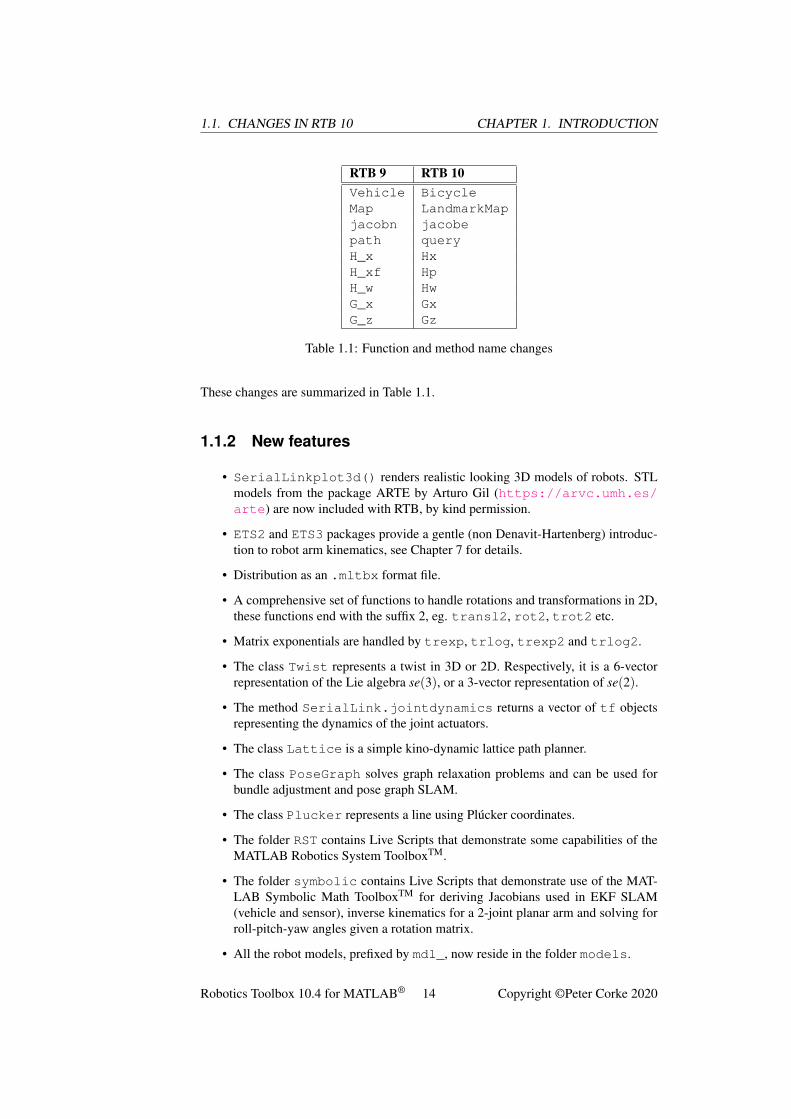
RTB 9 RTB 10Vehicle BicycleMap LandmarkMapjacobn jacobepath queryH_x HxH_xf HpH_w HwG_x GxG_z Gz
Table 1.1: Function and method name changes
These changes are summarized in Table 1.1.
1.1.2 New features
• SerialLinkplot3d() renders realistic looking 3D models of robots. STLmodels from the package ARTE by Arturo Gil (https://arvc.umh.es/arte) are now included with RTB, by kind permission.
• ETS2 and ETS3 packages provide a gentle (non Denavit-Hartenberg) introduc-tion to robot arm kinematics, see Chapter 7 for details.
• Distribution as an .mltbx format file.
• A comprehensive set of functions to handle rotations and transformations in 2D,these functions end with the suffix 2, eg. transl2, rot2, trot2 etc.
• Matrix exponentials are handled by trexp, trlog, trexp2 and trlog2.
• The class Twist represents a twist in 3D or 2D. Respectively, it is a 6-vectorrepresentation of the Lie algebra se(3), or a 3-vector representation of se(2).
• The method SerialLink.jointdynamics returns a vector of tf objectsrepresenting the dynamics of the joint actuators.
• The class Lattice is a simple kino-dynamic lattice path planner.
• The class PoseGraph solves graph relaxation problems and can be used forbundle adjustment and pose graph SLAM.
• The class Plucker represents a line using Plúcker coordinates.
• The folder RST contains Live Scripts that demonstrate some capabilities of theMATLAB Robotics System ToolboxTM.
• The folder symbolic contains Live Scripts that demonstrate use of the MAT-LAB Symbolic Math ToolboxTM for deriving Jacobians used in EKF SLAM(vehicle and sensor), inverse kinematics for a 2-joint planar arm and solving forroll-pitch-yaw angles given a rotation matrix.
• All the robot models, prefixed by mdl_, now reside in the folder models.
Robotics Toolbox 10.4 for MATLAB® 14 Copyright ©Peter Corke 2020
CHAPTER 1. INTRODUCTION 1.1. CHANGES IN RTB 10
• New robot models include Universal Robotics UR3, UR5 and UR10; and Kukalight weight robot arm.
• A new folder data now holds various data files as used by examples in RVC2:STL models, occupancy grids, Hershey font, Toro and G2O data files.
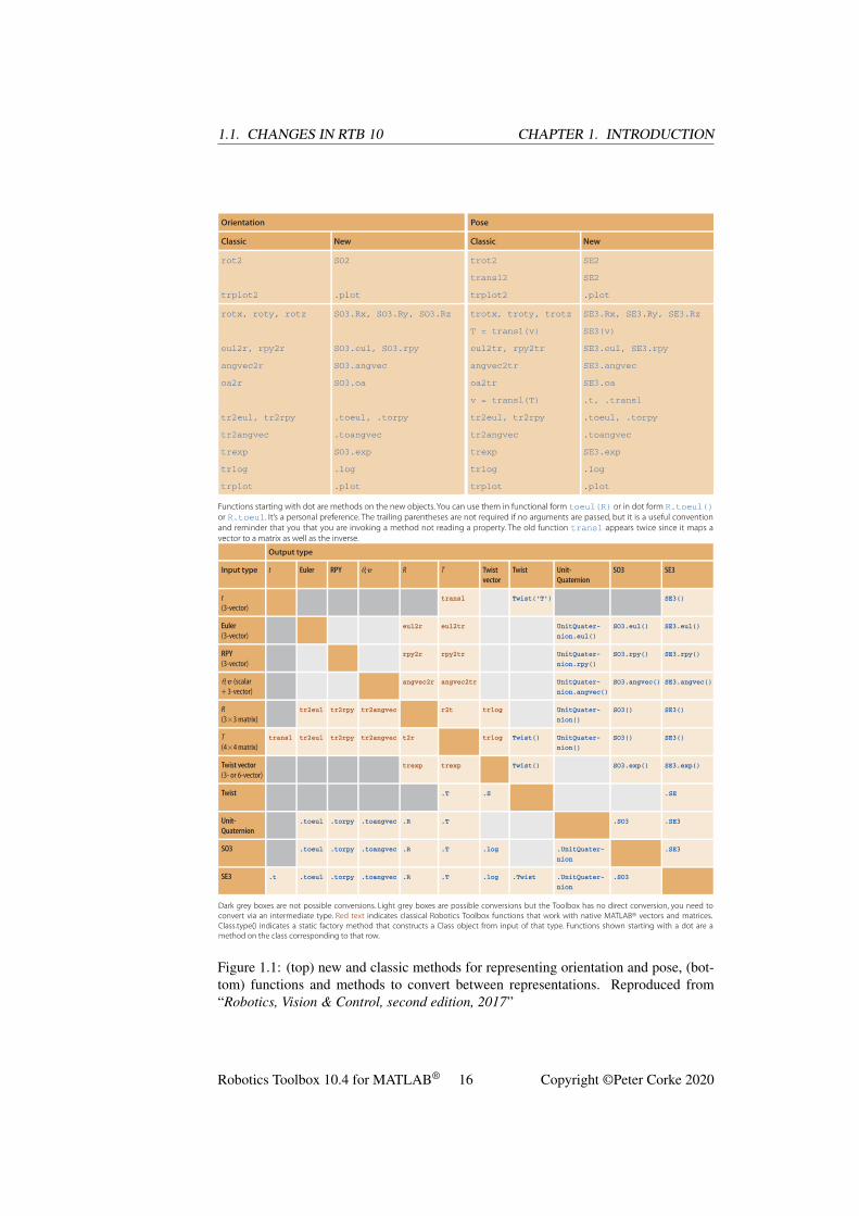
Since its inception RTB has used matrices1 to represent rotations and transformationsin 2D and 3D. A trajectory, or sequence, was represented by a 3-dimensional matrix,eg. 4× 4×N. In RTB10 a set of classes have been introduced to represent orienta-tion and pose in 2D and 3D: SO2, SE2, SO3, SE3, Twist and UnitQuaternion.These classes are fairly polymorphic, that is, they share many methods and operators2.All have a number of static methods that serve as constructors from particular repre-sentations. A trajectory is represented by a vector of these objects which makes codeeasier to read and understand. Overloaded operators are used so the classes behavein a similar way to native matrices3. The relationship between the classical Toolboxfunctions and the new classes are shown in Fig 1.1.
You can continue to use the classical functions. The new classes have methods withthe names of classical functions to provide similar functionality. For instance
>> T = transl(1,2,3); % create a 4x4 matrix>> trprint(T) % invoke the function trprint>> T = SE3(1,2,3); % create an SE3 object>> trprint(T) % invoke the method trprint>> T.T % the equivalent 4x4 matrix>> double(T) % the equivalent 4x4 matrix
>> T = SE3(1,2,3); % create a pure translation SE3 object>> T2 = T*T; % the result is an SE3 object>> T3 = trinterp(T, T2,, 5); % create a vector of five SE3 objects between T and T2>> T3(1) % the first element of the vector>> T3*T % each element of T3 multiplies T, giving a vector of five SE3 objects
1.1.3 Enhancements
• Dependencies on the Machine Vision Toolbox for MATLAB (MVTB) have beenremoved. The fast dilation function used for path planning is now searched forin MVTB and the MATLAB Image Processing Toolbox (IPT) and defaults to aprovided M-function.
• A major pass over all code and method/function/class documentation.
• Reworking and refactoring all the manipulator graphics, work in progress.
• An “app" is included: tripleangle which allows graphical experimentationwith Euler and roll-pitch-yaw angles.
• A tidyup of all Simulink models. Red blocks now represent user settable param-eters, and shaded boxes are used to group parts of the models.
1Early versions of RTB, before 1999, used vectors to represent quaternions but that changed to an objectonce objects were added to the language.
2For example, you could substitute objects of class SO3 and UnitQuaternion with minimal codechange.
3The capability is extended so that we can element-wise multiple two vectors of transforms, multiply onetransform over a vector of transforms or a set of points.
Robotics Toolbox 10.4 for MATLAB® 15 Copyright ©Peter Corke 2020
1.1. CHANGES IN RTB 10 CHAPTER 1. INTRODUCTION
Figure 1.1: (top) new and classic methods for representing orientation and pose, (bot-tom) functions and methods to convert between representations. Reproduced from“Robotics, Vision & Control, second edition, 2017”
Robotics Toolbox 10.4 for MATLAB® 16 Copyright ©Peter Corke 2020
CHAPTER 1. INTRODUCTION 1.2. CHANGES IN RTB 10.3
• RangeBearingSensor animation
• All the java code that supports the DHFactor functionality now lives in thefolder java. The Makefile in there can be used to recompile the code. Thereare java version issues and the shipped class files are built to java 1.7 whichallows operation
1.2 Changes in RTB 10.3
This release includes minor new features and a number of bug fixes compared to 10.2:
• Serial-link manipulators
– The Symbolic Robot Modeling Toolbox component by Jörn Malzahn hasbeen updated. It offers amazing speedups by using symbolic algebra tocreate robot specific MATLAB code or MEX files and it can even generateoptimised Simulink blocks. I’ve seen speedups of over 50,000x. You needto have the Symbolic Math Toolbox.
– New robot kinematic models: Franka-Emika PANDA and Rethink Sawyer.
– Methods DH and MDH on the SerialLink class convert models betweenDH and MDH kinematics. Dynamics not yet supported.
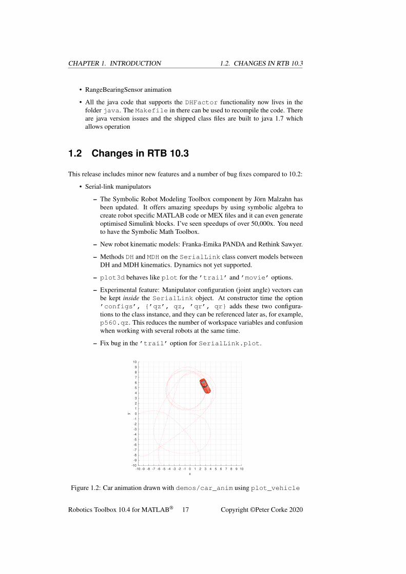
– plot3d behaves like plot for the ’trail’ and ’movie’ options.
– Experimental feature: Manipulator configuration (joint angle) vectors canbe kept inside the SerialLink object. At constructor time the option’configs’, {’qz’, qz, ’qr’, qr} adds these two configura-tions to the class instance, and they can be referenced later as, for example,p560.qz. This reduces the number of workspace variables and confusionwhen working with several robots at the same time.
– Fix bug in the ’trail’ option for SerialLink.plot.
-10 -9 -8 -7 -6 -5 -4 -3 -2 -1 0 1 2 3 4 5 6 7 8 9 10
x
-10
-9
-8
-7
-6
-5
-4
-3
-2
-1
0
1
2
3
4
5
6
7
8
9
10
y
Figure 1.2: Car animation drawn with demos/car_anim using plot_vehicle
Robotics Toolbox 10.4 for MATLAB® 17 Copyright ©Peter Corke 2020
1.2. CHANGES IN RTB 10.3 CHAPTER 1. INTRODUCTION
– Fixed bug in ikunc, ikcon which ignored q0.
• Mobile robotics
– Added the ability to animate a picture of a vehicle to plot_vehicle,see demos/car_demo and Figure 1.2. Also added a ’trail’ feature,and updated documentation.
– Experimental feature : A Reeds-Shepp path planner, see rReedsShepp.mand demos/reedsshepp.mlx, this is not (yet) properly integrated intothe Navigation class architecture.
• Simulink
– Simulink blocks for Euler angles now have a checkbox to allow degreesmode.
– Simulink blocks for roll-pitch-yaw angles now have a checkbox to allowdegrees mode and radio buttons to select the angle sequence.
– New Simulink block for mstraj gives full access to all capabilities of thatfunction.
– A folder simulink/R2015a contains all the Simulink models exportedas .slx files for Simulink R2015a. This might ease problems for thoseusing older versions of Simulink on the models in the top folder, many ofwhich have been edited and saved under R2018a. Check the README filefor details.
• A new script rvccheck which attempts to diagnose installation and MATLABpath issues.
• The demos folder now includes LiveScript versions of each demo, these are.mlx files. I’ve done a first pass at formatting the content and in a few casesupdating the content a little. From here on, the .m files are deprecated. You needMATLAB 2016a or later to run the LiveScripts.
• Major tidyup and documentation improvements for the Twist and Pluckerobjects.
• Changes to the RTBPose.mtimes method which now allows you to:
– postmultiply an SE3 object by a Plucker object which returns a Pluckerobject. This applies a rigid-body transformation to the line in space.
– postmultiply an SE2 object by a MATLAB polyshape object which re-turns a polyshape object. This applies a rigid-body transformation tothe polygon.
• Added a disp method to various toolbox objects, invokes display, whichprovides a display of the type from within the debugger.
• Quaternion == operator
• UnitQuaternion == accounts for double mapping
• UnitQuaternion has a rand method that generates a randomly distributedrotation, also used by SO3.rand and SE3.rand.
Robotics Toolbox 10.4 for MATLAB® 18 Copyright ©Peter Corke 2020
CHAPTER 1. INTRODUCTION 1.3. CHANGES IN RTB 10.2
• tr2rpy fixed a long standing bug with the pitch angle in certain corner cases,the pitch angle now lies in the range [−π,+π).
• Remove dependency on numrows() and numcols() for rt2tr, tr2rt,transl, transl2 which simplifies standalone operation.
• A campaign to reduce the size of the RTB distribution file:
– tripleangle uses updated STL files with reduced triangle counts forfaster loading.
– This manual is compressed.
– Removal of extraneous files.
• Options to RTB functions can now be strings or character arrays, ie. rotx(45,’deg’) or rotx(45, "deg"). If you don’t yet know about MATLABstrings (with double quotes) check them out.
• General tidyup to code and documentation, added missing files from earlier re-leases.
1.3 Changes in RTB 10.2
This release has a relatively small number of bug fixes compared to 10.1:
• Fixed bugs in jacobe and coriolis when using symbolic arguments.
• New robot models: UR3, UR5, UR10, LWR.
• Fixed bug for interp method of SE3 object.
• Fixed bug with detecting Optimisation Toolbox for ikcon and ikunc.
• Fixed bug in ikine_sym.
• Fixed various bugs related to plotting robots with prismatic joints.
1.4 How to obtain the Toolbox
The Robotics Toolbox is freely available from the Toolbox home page at
http://www.petercorke.com
The file is available in MATLABtoolbox format (.mltbx) or zip format (.zip).
1.4.1 From .mltbx file
Since MATLAB R2014b toolboxes can be packaged as, and installed from, files withthe extension .mltbx. Download the most recent version of robot.mltbx orvision.mltbx to your computer. Using MATLAB navigate to the folder whereyou downloaded the file and double-click it (or right-click then select Install). The
Robotics Toolbox 10.4 for MATLAB® 19 Copyright ©Peter Corke 2020
1.4. HOW TO OBTAIN THE TOOLBOX CHAPTER 1. INTRODUCTION
Toolbox will be installed within the local MATLAB file structure, and the paths will beappropriately configured for this, and future MATLAB sessions.
1.4.2 From .zip file
Download the most recent version of robot.zip or vision.zip to your computer. Useyour favourite unarchiving tool to unzip the files that you downloaded. To add theToolboxes to your MATLAB path execute the command
>> addpath RVCDIR ;>> startup_rvc
where RVCDIR is the full pathname of the folder where the folder rvctools wascreated when you unzipped the Toolbox files. The script startup_rvc adds varioussubfolders to your path and displays the version of the Toolboxes. After installationthe files for both Toolboxes reside in a top-level folder called rvctools and beneaththis are a number of folders:
robot The Robotics Toolboxvision The Machine Vision Toolboxcommon Utility functions common to the Robotics and Machine Vision Toolboxessimulink Simulink blocks for robotics and vision, as well as examplescontrib Code written by third-parties
If you already have the Machine Vision Toolbox installed then download the zip file tothe folder above the existing rvctools directory, and then unzip it. The files fromthis zip archive will properly interleave with the Machine Vision Toolbox files.
You need to setup the path every time you start MATLAB but you can automate this bysetting up environment variables, editing your startup.m script, using pathtooland saving the path, or by pressing the “Update Toolbox Path Cache" button underMATLAB General preferences. You can check the path using the command path orpathtool.
A menu-driven demonstration can be invoked by
>> rtbdemo
1.4.3 MATLAB OnlineTM
The Toolbox works well with MATLAB OnlineTM which lets you access a MATLABsession from a web browser, tablet or even a phone. The key is to get the RTB filesinto the filesystem associated with your Online account. The easiest way to do this isto install MATLAB DriveTM from MATLAB File Exchange or using the Get Add-Onsoption from the MATLAB GUI. This functions just like Google Drive or Dropbox,a local filesystem on your computer is synchronized with your MATLAB Online ac-count. Copy the RTB files into the local MATLAB Drive cache and they will soon besynchronized, invoke startup_rvc to setup the paths and you are ready to simulaterobots on your mobile device or in a web browser.
Robotics Toolbox 10.4 for MATLAB® 20 Copyright ©Peter Corke 2020
CHAPTER 1. INTRODUCTION 1.4. HOW TO OBTAIN THE TOOLBOX
(a) (b)
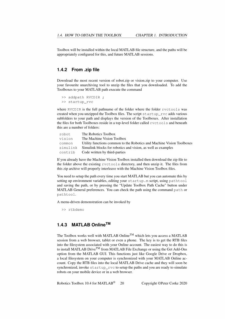
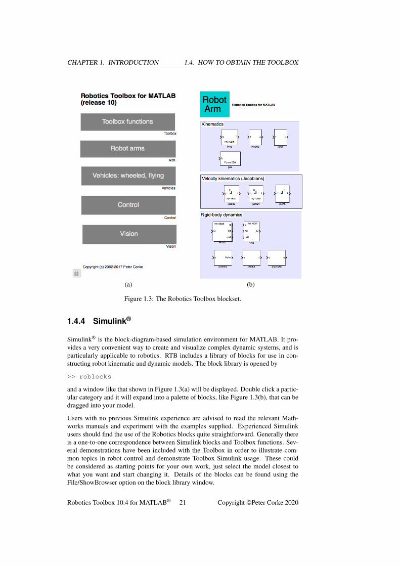
Figure 1.3: The Robotics Toolbox blockset.
1.4.4 Simulink®
Simulink® is the block-diagram-based simulation environment for MATLAB. It pro-vides a very convenient way to create and visualize complex dynamic systems, and isparticularly applicable to robotics. RTB includes a library of blocks for use in con-structing robot kinematic and dynamic models. The block library is opened by
>> roblocks
and a window like that shown in Figure 1.3(a) will be displayed. Double click a partic-ular category and it will expand into a palette of blocks, like Figure 1.3(b), that can bedragged into your model.
Users with no previous Simulink experience are advised to read the relevant Math-works manuals and experiment with the examples supplied. Experienced Simulinkusers should find the use of the Robotics blocks quite straightforward. Generally thereis a one-to-one correspondence between Simulink blocks and Toolbox functions. Sev-eral demonstrations have been included with the Toolbox in order to illustrate com-mon topics in robot control and demonstrate Toolbox Simulink usage. These couldbe considered as starting points for your own work, just select the model closest towhat you want and start changing it. Details of the blocks can be found using theFile/ShowBrowser option on the block library window.
Robotics Toolbox 10.4 for MATLAB® 21 Copyright ©Peter Corke 2020
1.4. HOW TO OBTAIN THE TOOLBOX CHAPTER 1. INTRODUCTION
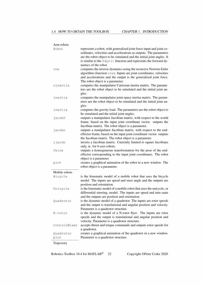
Arm robotsRobot represents a robot, with generalized joint force input and joint co-
ordinates, velocities and accelerations as outputs. The parametersare the robot object to be simulated and the initial joint angles. Itis similar to the fdyn() function and represents the forward dy-namics of the robot.
rne computes the inverse dynamics using the recursive Newton-Euleralgorithm (function rne). Inputs are joint coordinates, velocitiesand accelerations and the output is the generalized joint force.The robot object is a parameter.
cinertia computes the manipulator Cartesian inertia matrix. The parame-ters are the robot object to be simulated and the initial joint an-gles.
inertia computes the manipulator joint-space inertia matrix. The param-eters are the robot object to be simulated and the initial joint an-gles.
inertia computes the gravity load. The parameters are the robot object tobe simulated and the initial joint angles.
jacob0 outputs a manipulator Jacobian matrix, with respect to the worldframe, based on the input joint coordinate vector. outputs theJacobian matrix. The robot object is a parameter.
jacobn outputs a manipulator Jacobian matrix, with respect to the end-effector frame, based on the input joint coordinate vector. outputsthe Jacobian matrix. The robot object is a parameter.
ijacob inverts a Jacobian matrix. Currently limited to square Jacobiansonly, ie. for 6-axis robots.
fkine outputs a homogeneous transformation for the pose of the end-effector corresponding to the input joint coordinates. The robotobject is a parameter.
plot creates a graphical animation of the robot in a new window. Therobot object is a parameter.
Mobile robotsBicycle is the kinematic model of a mobile robot that uses the bicycle
model. The inputs are speed and steer angle and the outputs areposition and orientation.
Unicycle is the kinematic model of a mobile robot that uses the unicycle, ordifferential steering, model. The inputs are speed and turn raateand the outputs are position and orientation.
Quadrotor is the dynamic model of a quadrotor. The inputs are rotor speedsand the output is translational and angular position and velocity.Parameter is a quadrotor structure.
N-rotor is the dynamic model of a N-rotor flyer. The inputs are rotorspeeds and the output is translational and angular position andvelocity. Parameter is a quadrotor structure.
ControlMixer accepts thrust and torque commands and outputs rotor speeds fora quadrotor.
Quadrotorplot
creates a graphical animation of the quadrotor in a new window.Parameter is a quadrotor structure.
Trajectory
Robotics Toolbox 10.4 for MATLAB® 22 Copyright ©Peter Corke 2020
CHAPTER 1. INTRODUCTION 1.4. HOW TO OBTAIN THE TOOLBOX
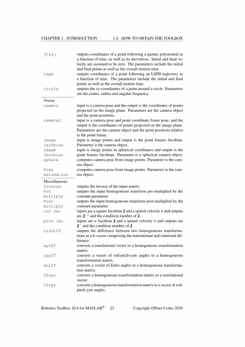
jtraj outputs coordinates of a point following a quintic polynomial asa function of time, as well as its derivatives. Initial and final ve-locity are assumed to be zero. The parameters include the initialand final points as well as the overall motion time.
lspb outputs coordinates of a point following an LSPB trajectory asa function of time. The parameters include the initial and finalpoints as well as the overall motion time.
circle outputs the xy-coordinates of a point around a circle. Parametersare the centre, radius and angular frequency.
Visioncamera input is a camera pose and the output is the coordinates of points
projected on the image plane. Parameters are the camera objectand the point positions.
camera2 input is a camera pose and point coordinate frame pose, and theoutput is the coordinates of points projected on the image plane.Parameters are the camera object and the point positions relativeto the point frame.
imageJacobian
input is image points and output is the point feature Jacobian.Parameter is the camera object.
imageJacobiansphere
input is image points in spherical coordinates and output is thepoint feature Jacobian. Parameter is a spherical camera object.computes camera pose from image points. Parameter is the cam-era object.
Poseestimation
computes camera pose from image points. Parameter is the cam-era object.
MiscellaneousInverse outputs the inverse of the input matrix.Premultiply
outputs the input homogeneous transform pre-multiplied by theconstant parameter.
Postmultiply
outputs the input homogeneous transform post-multiplied by theconstant parameter.
inv Jac inputs are a square Jacobian J and a spatial velocity ν and outputsare J−1 and the condition number of J.
pinv Jac inputs are a Jacobian J and a spatial velocity ν and outputs areJ+ and the condition number of J.
tr2diff outputs the difference between two homogeneous transforma-tions as a 6-vector comprising the translational and rotational dif-ference.
xyz2T converts a translational vector to a homogeneous transformationmatrix.
rpy2T converts a vector of roll-pitch-yaw angles to a homogeneoustransformation matrix.
eul2T converts a vector of Euler angles to a homogeneous transforma-tion matrix.
T2xyz converts a homogeneous transformation matrix to a translationalvector.
T2rpy converts a homogeneous transformation matrix to a vector of roll-pitch-yaw angles.
Robotics Toolbox 10.4 for MATLAB® 23 Copyright ©Peter Corke 2020
1.4. HOW TO OBTAIN THE TOOLBOX CHAPTER 1. INTRODUCTION
T2eul converts a homogeneous transformation matrix to a vector of Eu-ler angles.
angdiff computes the difference between two input angles modulo 2π .
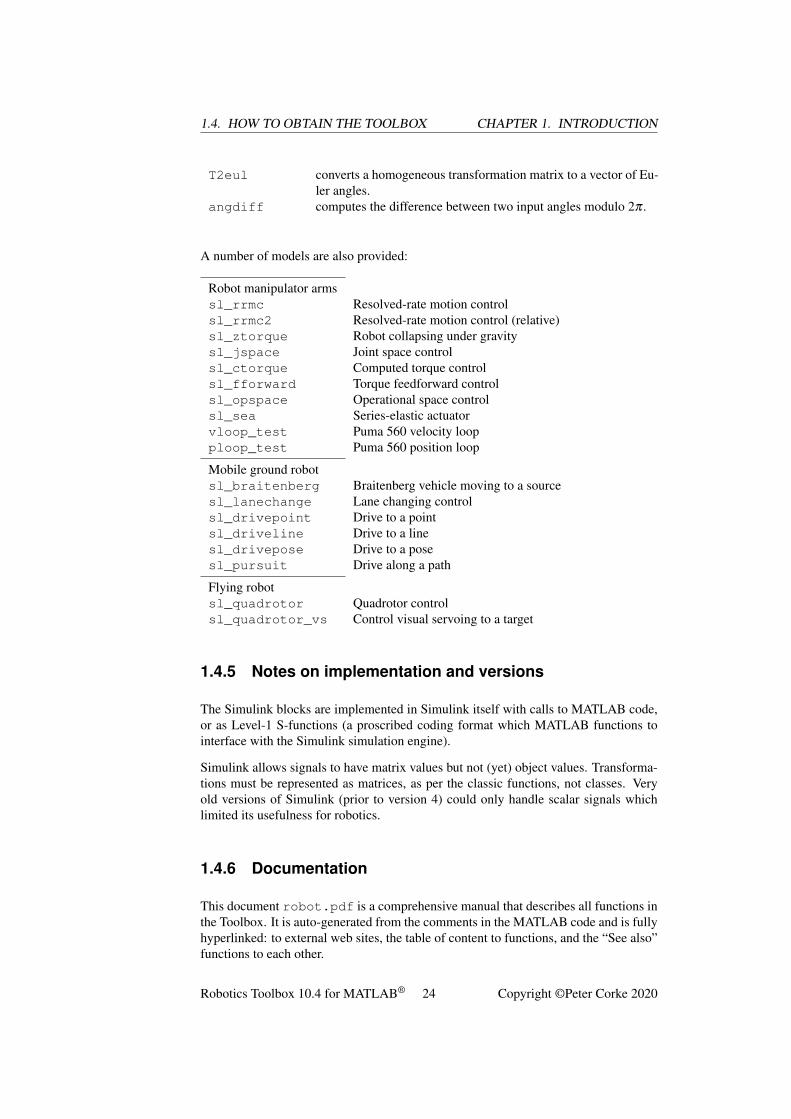
A number of models are also provided:
Robot manipulator armssl_rrmc Resolved-rate motion controlsl_rrmc2 Resolved-rate motion control (relative)sl_ztorque Robot collapsing under gravitysl_jspace Joint space controlsl_ctorque Computed torque controlsl_fforward Torque feedforward controlsl_opspace Operational space controlsl_sea Series-elastic actuatorvloop_test Puma 560 velocity loopploop_test Puma 560 position loop
Mobile ground robotsl_braitenberg Braitenberg vehicle moving to a sourcesl_lanechange Lane changing controlsl_drivepoint Drive to a pointsl_driveline Drive to a linesl_drivepose Drive to a posesl_pursuit Drive along a path
Flying robotsl_quadrotor Quadrotor controlsl_quadrotor_vs Control visual servoing to a target
1.4.5 Notes on implementation and versions
The Simulink blocks are implemented in Simulink itself with calls to MATLAB code,or as Level-1 S-functions (a proscribed coding format which MATLAB functions tointerface with the Simulink simulation engine).
Simulink allows signals to have matrix values but not (yet) object values. Transforma-tions must be represented as matrices, as per the classic functions, not classes. Veryold versions of Simulink (prior to version 4) could only handle scalar signals whichlimited its usefulness for robotics.
1.4.6 Documentation
This document robot.pdf is a comprehensive manual that describes all functions inthe Toolbox. It is auto-generated from the comments in the MATLAB code and is fullyhyperlinked: to external web sites, the table of content to functions, and the “See also”functions to each other.
Robotics Toolbox 10.4 for MATLAB® 24 Copyright ©Peter Corke 2020
CHAPTER 1. INTRODUCTION 1.5. COMPATIBLE MATLAB VERSIONS
1.5 Compatible MATLAB versions
The Toolbox has been tested under R2019b and R2020aPRE. Compatibility problemsare increasingly likely the older your version of MATLAB is.
1.6 Use in teaching
This is definitely encouraged! You are free to put the PDF manual (robot.pdf orthe web-based documentation html/*.html on a server for class use. If you plan todistribute paper copies of the PDF manual then every copy must include the first twopages (cover and licence).
Link to other resources such as MOOCs or the Robot Academy can be found at www.petercorke.com/moocs.
1.7 Use in research
If the Toolbox helps you in your endeavours then I’d appreciate you citing the Toolboxwhen you publish. The details are:
@book{Corke17a,Author = {Peter I. Corke},Note = {ISBN 978-3-319-54413-7},Edition = {Second},Publisher = {Springer},Title = {Robotics, Vision \& Control: Fundamental Algorithms in {MATLAB}},Year = {2017}}
or
P.I. Corke, Robotics, Vision & Control: Fundamental Algorithms in MAT-LAB. Second edition. Springer, 2017. ISBN 978-3-319-54413-7.
which is also given in electronic form in the CITATION file.
1.8 Support
There is no support! This software is made freely available in the hope that you find ituseful in solving whatever problems you have to hand. I am happy to correspond withpeople who have found genuine bugs or deficiencies but my response time can be longand I can’t guarantee that I respond to your email.
I can guarantee that I will not respond to any requests for help with assignmentsor homework, no matter how urgent or important they might be to you. That’swhat your teachers, tutors, lecturers and professors are paid to do.
You might instead like to communicate with other users via the Google Group called“Robotics and Machine Vision Toolbox”
Robotics Toolbox 10.4 for MATLAB® 25 Copyright ©Peter Corke 2020
1.9. RELATED SOFTWARE CHAPTER 1. INTRODUCTION
http://tiny.cc/rvcforum
which is a forum for discussion. You need to signup in order to post, and the signupprocess is moderated by me so allow a few days for this to happen. I need you to write afew words about why you want to join the list so I can distinguish you from a spammeror a web-bot.
1.9 Related software
1.9.1 Robotics System ToolboxTM
The Robotics System ToolboxTM (RST) from MathWorks is an official and supportedproduct. System toolboxes (see also the Computer Vision System Toolbox) are aimedat developers of systems. RST has a growing set of functions for mobile robots, armrobots, ROS integration and pose representations but its design (classes and functions)and syntax is quite different to RTB. A number of examples illustrating the use of RSTare given in the folder RST as Live Scripts (extension .mlx), but you need to have theRobotics System ToolboxTM installed in order to use it.
1.9.2 Octave
GNU Octave (www.octave.org) is an impressive piece of free software that implementsa language that is close to, but not the same as, MATLAB. The Toolboxes currently donot work well with Octave, though as time goes by compatibility improves. ManyToolbox functions work just fine under Octave, but most classes do not.
For uptodate information about running the Toolbox with Octave check out the pagehttp://petercorke.com/wordpress/toolboxes/other-languages.
1.9.3 Machine Vision toolbox
Machine Vision toolbox (MVTB) for MATLAB. This was described in an article
@article{Corke05d,Author = {P.I. Corke},Journal = {IEEE Robotics and Automation Magazine},Month = nov,Number = {4},Pages = {16-25},Title = {Machine Vision Toolbox},Volume = {12},Year = {2005}}
and provides a very wide range of useful computer vision functions and is used to il-lustrate principals in the Robotics, Vision & Control book. You can obtain this fromhttp://www.petercorke.com/vision. More recent products such as MAT-LAB Image Processing Toolbox and MATLAB Computer Vision System Toolbox pro-vide functionality that overlaps with MVTB.
Robotics Toolbox 10.4 for MATLAB® 26 Copyright ©Peter Corke 2020
CHAPTER 1. INTRODUCTION 1.10. CONTRIBUTING TO THE TOOLBOXES
1.10 Contributing to the Toolboxes
I am very happy to accept contributions for inclusion in future versions of the toolbox.You will, of course, be suitably acknowledged (see below).
1.11 Acknowledgements
I have corresponded with a great many people via email since the first release of thisToolbox. Some have identified bugs and shortcomings in the documentation, and evenbetter, some have provided bug fixes and even new modules, thankyou. See the fileCONTRIB for details.
I would especially like to thank the following. Giorgio Grisetti and Gian Diego Tipaldifor the core of the pose graph solver. Arturo Gil for allowing me to ship the STLrobot models from ARTE. Jörn Malzahn has donated a considerable amount of code,his Robot Symbolic Toolbox for MATLAB. Bryan Moutrie has contributed parts of hisopen-source package phiWARE to RTB, the remainder of that package can be foundonline. Other special mentions to Gautam Sinha, Wynand Smart for models of indus-trial robot arm, Pauline Pounds for the quadrotor and related models, Paul Newmanfor inspiring the mobile robot code, and Giorgio Grissetti for inspiring the pose graphcode.
Robotics Toolbox 10.4 for MATLAB® 27 Copyright ©Peter Corke 2020

1.11. ACKNOWLEDGEMENTS CHAPTER 1. INTRODUCTION
Robotics Toolbox 10.4 for MATLAB® 28 Copyright ©Peter Corke 2020
Chapter 2
Functions and classes
Astars
A* navigation class
A concrete subclass of the Navigation class that implements the A* navigationalgorithm. Methods included are for the standard case, multiobjective optimization(MOO) – i.e. optimizes over several objectives/criteria – and the A*-PO algorithms forMOO that utilizes Pareto optimality.
Methods:
plan Compute the cost map given a goal and mappath Compute a path to the goalvisualize Display the obstacle map (deprecated)plot Display the obstacle map
costmap_modify Modify the costmap
costmap_get Return the current costmapcostmap_set Set the current costmapdisplay Print the parameters in human readable formchar Convert to string
Properties: TBD
Example 1
load map1 % load mapgoal = [50;30];
Robotics Toolbox 10.4 for MATLAB® 29 Copyright ©Peter Corke 2020
CHAPTER 2. FUNCTIONS AND CLASSES
start=[20;10];as = Astar(map); % create Navigation objectas.plan(goal,2,3,0); % setup costmap for specified goal;
% standard D* algorithm w/ 2 objectives% and 3 costmap layers
as.path(start); % plan solution path start-to-goal, animateP = as.path(start); % plan solution path start-to-goal, return
% path
Example 2
goal = [100;100];start = [1;1];as = Astar(0); % create Navigation object with pseudo-
% random occupancy grid
ds.addCost(terrain); % terrain is a 100x100 matrix of
% elevations [0,1]
ds.plan(goal,3,4,0); % setup costmap for specified goal
% (3 and 4 include the added terrain cost)
as.path(start); % plan solution path start-goal, animateP = as.path(start); % plan solution path start-goal, return
% path
Notes
• Obstacles are represented by Inf in the costmap.
References
• A Pareto Optimal D* Search Algorithm for Multiobjective Path Planning, A.Lavin.
• A Pareto Front-Based Multiobjective Path Planning Algorithm, A. Lavin.
• Robotics, Vision & Control, Sec 5.2.2, Peter Corke, Springer, 2011.
See Also Navigation, Dstar
Astar.AstarA* constructor
AS = Astar(MAP, OPTIONS) is a A* navigation object, and MAP is an occu-pancy grid, a representation of a planar world as a matrix whose elements are 0 (freespace) or 1 (occupied). The occupancy grid is coverted to a costmap with a unit costfor traversing a cell.
Robotics Toolbox 10.4 for MATLAB® 30 Copyright ©Peter Corke 2020
CHAPTER 2. FUNCTIONS AND CLASSES
Options
'world'= 0 will call for a pseudo-random occupancy grid'goal',G Specify the goal point (2×1)'metric',M (default) or 'cityblock' Specify the distance metric as 'Euclidean''inflate',K Inflate all obstacles by K cells'quiet' Don't display the progress spinner
Other options are supported by the Navigation superclass.
See also
Navigation.Navigation
Astar.addCostAdd an additional cost layer
AS.addCost(values) adds the matrix specified by values as a cost layer. Inputs
values: normalized matrix the size of the environment
Astar.charConvert Navigation object to string
AS.char() is a string representing the state of the Astar object in human-readableform.
See also
Astar.display, Navigation.char
Astar.cost_getGet the specified cost layer
Robotics Toolbox 10.4 for MATLAB® 31 Copyright ©Peter Corke 2020
CHAPTER 2. FUNCTIONS AND CLASSES
Astar.costmap_getGet the current costmap
C = AS.costmap_get() is the current costmap. The value of each element rep-resents the cost of traversing the cell. It is autogenerated by the class constructor fromthe occupancy grid such that:
• free cell (occupancy 0) has a cost of 1
• occupied cell (occupancy >0) has a cost of Inf
See also
Astar.costmap_set, Astar.costmap_modify
Astar.costmap_modifyModify cost map
AS.costmap_modify(P, NEW) modifies the cost map at P=[X,Y] to have thevalue NEW. If P (2×M) and NEW (1×M) then the cost of the points defined by thecolumns of P are set to the corresponding elements of NEW.
Notes
• After one or more point costs have been updated the path should be replannedby calling AS.plan().
See also
Astar.costmap_set, Astar.costmap_get
Astar.costmap_setSet the current costmap
AS.costmap_set(C) sets the current costmap. This method accepts the full costmap– i.e. all layers.
Notes:
• After the cost map is changed the path should be replanned by calling AS.plan().
Robotics Toolbox 10.4 for MATLAB® 32 Copyright ©Peter Corke 2020
CHAPTER 2. FUNCTIONS AND CLASSES
See also
Astar.costmap_get, Astar.costmap_modify
Astar.dcthe distance cost of moving from state X to state Y
Astar.goal_changeChanges the costlayers due to new goal
position
Astar.heurstic_getGet the current heuristic map
C = AS.heuristice_get() is the current heuristic layer. It is computed in As-tar.plan.
See also
Astar.plan
Astar.INSERTstate X to the openlist with objective space values
specified by pt.
Astar.neighborsindices of neighbor states (max 8) as a row vector
Robotics Toolbox 10.4 for MATLAB® 33 Copyright ©Peter Corke 2020
CHAPTER 2. FUNCTIONS AND CLASSES
Astar.nextby Navigation.step
Backpropagate from goal to start Return [col;row] of previous step
Astar.pathFind a path between two points
AS.path(START) finds and displays a path from START to GOAL which is overlaidon the occupancy grid.
P = AS.path(START) returns the path (2×M) from START to GOAL.
Astar.planPrep the grid for planning.
AS.plan() updates AS with a costmap of distance to the goal from every non-obstacle point in the map. The goal is as specified to the constructor.
Inputs:
goal: goal state coordinates N: number of optimization objectives; standard A* is 2(i.e. distance and heuristic) layers: number of cost layers in costmap algorithm: specifystandard A*(0), A*-MOO (1), A*-PO (2)
Astar.plotVisualize navigation environment
AS.plot() displays the occupancy grid and the goal distance in a new figure. Thegoal distance is shown by intensity which increases with distance from the goal. Ob-stacles are overlaid and shown in red.
AS.plot(P) as above but also overlays a path given by the set of points P (M×2).
See also
Navigation.plot
Robotics Toolbox 10.4 for MATLAB® 34 Copyright ©Peter Corke 2020
CHAPTER 2. FUNCTIONS AND CLASSES
Astar.projectCostthe projection of state a into objective space. If
specified, location is moving from b to a (case 3).
Astar.resetReset the planner
AS.reset() resets the A* planner. The next instantiation of AS.plan() will performa global replan.
Astar.updateCostsOnly for costs that accumulate (i.e. sum) over the
path, and for dynamic costs. E.g. the heuristic parameter only needs updating whenthe goal state changes; its values are stored for each cell.
Location moving from state b to a.
The costs are coded to be (1) distance, (2) heuristic, (3) elevation, (4) solar devia-tion, and (5) risk. If deviating from these costs (in this order) you MUST EDIT THISMETHOD.
Astar.vcthe robot unit vector – direction of moving from
state X to state Y
AstarMOOA*-MOO navigation class
A concrete subclass of the Navigation class that implements the A* navigation al-gorithm for multiobjective optimization (MOO) - i.e. optimizes over several objec-
Robotics Toolbox 10.4 for MATLAB® 35 Copyright ©Peter Corke 2020
CHAPTER 2. FUNCTIONS AND CLASSES
tives/criteria.
Methods:
plan Compute the cost map given a goal and mappath Compute a path to the goalvisualize Display the obstacle map (deprecated)plot Display the obstacle mapcostmap_modify Modify the costmapcostmap_get Return the current costmapcostmap_set Set the current costmapdistancemap_get Set the current distance mapheuristic_get Get the current heuristic mapdisplay Print the parameters in human readable formchar Convert to string
Properties: TBD
Example
load map1 % load mapgoal = [50;30];start = [20;10];as = AstarMOO(map); % create Navigation objectas.plan(goal,2); % setup costmap for specified goalas.path(start); % plan solution path star-goal, animateP = as.path(start); % plan solution path star-goal, return path
Example 2:
goal = [100;100];start = [1;1];as = AstarMOO(0); % create Navigation object with random occupancy gridas.addCost(1,L); % add 1st add’l cost layer Las.plan(goal,3); % setup costmap for specified goalas.path(start); % plan solution path start-goal, animateP = as.path(start); % plan solution path start-goal, return path
Notes
• Obstacles are represented by Inf in the costmap.
References
• A Pareto Optimal D* Search Algorithm for Multiobjective Path Planning, A.Lavin.
• A Pareto Front-Based Multiobjective Path Planning Algorithm, A. Lavin.
• Robotics, Vision & Control, Sec 5.2.2, Peter Corke, Springer, 2011.
Robotics Toolbox 10.4 for MATLAB® 36 Copyright ©Peter Corke 2020
CHAPTER 2. FUNCTIONS AND CLASSES
Author
Alexander Lavin
See also
Navigation, Astar, AstarPO
AstarMOO.AstarMOOA*-MOO constructor
AS = AstarMOO(MAP, OPTIONS) is a A* navigation object, and MAP is an oc-cupancy grid, a representation of a planar world as a matrix whose elements are 0 (freespace) or 1 (occupied). The occupancy grid is coverted to a costmap with a unit costfor traversing a cell.
Options
'goal',G Specify the goal point (2×1)'metric',M or 'cityblock'. Specify the distance metric as 'euclidean'(default)'inflate',K Inflate all obstacles by K cells.'quiet' Don't display the progress spinner
Other options are supported by the Navigation superclass.
Notes
• If MAP == 0 a random map is created.
See also
Navigation.Navigation
AstarMOO.addCostAdd an additional cost layer
AS.addCost(LAYER, VALUES) adds the matrix specified by values as a costlayer. The layer number is given by LAYER, and VALUES has the same size as the
Robotics Toolbox 10.4 for MATLAB® 37 Copyright ©Peter Corke 2020
CHAPTER 2. FUNCTIONS AND CLASSES
original occupancy grid.
AstarMOO.charConvert navigation object to string
AS.char() is a string representing the state of the Astar object in human-readableform.
See also
AstarMOO.display, Navigation.char
AstarMOO.cost_getGet the specified cost layer
AstarMOO.costmap_getGet the current costmap
C = AS.costmap_get() is the current costmap. The cost map is the same size asthe occupancy grid and the value of each element represents the cost of traversing thecell. It is autogenerated by the class constructor from the occupancy grid such that:
• free cell (occupancy 0) has a cost of 1
• occupied cell (occupancy >0) has a cost of Inf
See also
Astar.costmap_set, Astar.costmap_modify
AstarMOO.costmap_modifyModify cost map
AS.costmap_modify(P, NEW) modifies the cost map at P=[X,Y] to have thevalue NEW. If P (2×M) and NEW (1×M) then the cost of the points defined by thecolumns of P are set to the corresponding elements of NEW.
Robotics Toolbox 10.4 for MATLAB® 38 Copyright ©Peter Corke 2020
CHAPTER 2. FUNCTIONS AND CLASSES
Notes
• After one or more point costs have been updated the path should be replannedby calling AS.plan().
See also
AstarMOO.costmap_set, AstarMOO.costmap_get
AstarMOO.costmap_setSet the current costmap
AS.costmap_set(C) sets the current costmap. The cost map is the same size asthe occupancy grid and the value of each element represents the cost of traversing thecell. A high value indicates that the cell is more costly (difficult) to traverese. A valueof Inf indicates an obstacle.
Notes
• After the cost map is changed the path should be replanned by calling AS.plan().
See also
Astar.costmap_get, Astar.costmap_modify
AstarMOO.heuristic_getGet the current heuristic map
C = AS.heuristic_get() is the current heuristic map. This map is the samesize as the occupancy grid and the value of each element is the shortest distance fromthe corresponding point in the map to the current goal. It is computed by Astar.plan.
See also
Astar.plan
Robotics Toolbox 10.4 for MATLAB® 39 Copyright ©Peter Corke 2020
CHAPTER 2. FUNCTIONS AND CLASSES
AstarMOO.nextfrom goal to start
Return [col;row] of previous step
AstarMOO.pathFind a path between two points
AS.path(START) finds and displays a path from START to GOAL which is overlaidon the occupancy grid.
P = AS.path(START) returns the path (2×M) from START to GOAL.
AstarMOO.planPrep the grid for planning.
AS.plan() updates AS with a costmap of distance to the goal from every non-obstacle point in the map. The goal is as specified to the constructor.
Inputs:
goal: goal state coordinates N: number of optimization objectives; standard A* is 2(i.e. distance and heuristic)
AstarMOO.plotVisualize navigation environment
AS.plot() displays the occupancy grid and the goal distance in a new figure. Thegoal distance is shown by intensity which increases with distance from the goal. Ob-stacles are overlaid and shown in red.
AS.plot(P) as above but also overlays a path given by the set of points P (M×2).
See also
Navigation.plot
Robotics Toolbox 10.4 for MATLAB® 40 Copyright ©Peter Corke 2020
CHAPTER 2. FUNCTIONS AND CLASSES
AstarMOO.resetReset the planner
AS.reset() resets the A* planner. The next instantiation of AS.plan() will performa global replan.
AstarPO(A*-PO)
A*PO navigation class
A concrete subclass of the Navigation class that implements the A* navigation al-gorithm for multiobjective optimization (MOO) - i.e. optimizes over several objec-tives/criteria.
Methods
plan Compute the cost map given a goal and mappath Compute a path to the goalvisualize Display the obstacle map (deprecated)plot Display the obstacle map
costmap_modify Modify the costmap
costmap_get Return the current costmapcostmap_set Set the current costmapdistancemap_get Set the current distance mapheuristic_get Get the current heuristic mapdisplay Print the parameters in human readable formchar Convert to string
Properties
TBD
Example
Robotics Toolbox 10.4 for MATLAB® 41 Copyright ©Peter Corke 2020
CHAPTER 2. FUNCTIONS AND CLASSES
load map1 % load map
goal = [50;30];start = [20;10];as = AstarPO(map); % create Navigation objectas.plan(goal,2); % setup costmap for specified goalas.path(start); % plan solution path star-goal, animateP = as.path(start); % plan solution path star-goal, return path
Example 2:
goal = [100;100];start = [1;1];as = AstarPO(0); % create Navigation object with random occupancy gridas.addCost(1,L); % add 1st add’l cost layer Las.plan(goal,3); % setup costmap for specified goalas.path(start); % plan solution path start-goal, animateP = as.path(start); % plan solution path start-goal, return path
Notes
• Obstacles are represented by Inf in the costmap.
References
• A Pareto Optimal D* Search Algorithm for Multiobjective Path Planning, A.Lavin.
• A Pareto Front-Based Multiobjective Path Planning Algorithm, A. Lavin.
• Robotics, Vision & Control, Sec 5.2.2, Peter Corke, Springer, 2011.
Author
Alexander Lavin
See also
Navigation, Astar, AstarMOO
AstarPO.AstarPOA*-PO constructor
AS = AstarPO(MAP, OPTIONS) is a A* navigation object, and MAP is an occu-pancy grid, a representation of a planar world as a matrix whose elements are 0 (free
Robotics Toolbox 10.4 for MATLAB® 42 Copyright ©Peter Corke 2020
CHAPTER 2. FUNCTIONS AND CLASSES
space) or 1 (occupied). The occupancy grid is coverted to a costmap with a unit costfor traversing a cell.
Options
'world'= 0 will call for a random occupancy grid to be built'goal',G Specify the goal point (2×1)'metric',M or 'cityblock'. Specify the distance metric as 'euclidean'(default)'inflate',K Inflate all obstacles by K cells.'quiet' Don't display the progress spinner
Other options are supported by the Navigation superclass.
See also
Navigation.Navigation
AstarPO.addCost
Add an additional cost layer
AS.addCost(LAYER, VALUES) adds the matrix specified by values as a costlayer. The layer number is given by LAYER, and VALUES has the same size as theoriginal occupancy grid.
AstarPO.char
Convert navigation object to string
AS.char() is a string representing the state of the Astar object in human-readableform.
See also
AstarMOO.display, Navigation.char
Robotics Toolbox 10.4 for MATLAB® 43 Copyright ©Peter Corke 2020
CHAPTER 2. FUNCTIONS AND CLASSES
AstarPO.cost_get
Get the specified cost layer
AstarPO.costmap_get
Get the current costmap
C = AS.costmap_get() is the current costmap. The cost map is the same size asthe occupancy grid and the value of each element represents the cost of traversing thecell. It is autogenerated by the class constructor from the occupancy grid such that:
• free cell (occupancy 0) has a cost of 1
• occupied cell (occupancy >0) has a cost of Inf
See also
Astar.costmap_set, Astar.costmap_modify
AstarPO.costmap_modify
Modify cost map
AS.costmap_modify(P, NEW) modifies the cost map at P=[X,Y] to have thevalue NEW. If P (2×M) and NEW (1×M) then the cost of the points defined by thecolumns of P are set to the corresponding elements of NEW.
Notes
• After one or more point costs have been updated the path should be replannedby calling AS.plan().
See also
AstarMOO.costmap_set, AstarMOO.costmap_get
Robotics Toolbox 10.4 for MATLAB® 44 Copyright ©Peter Corke 2020
CHAPTER 2. FUNCTIONS AND CLASSES
AstarPO.costmap_setSet the current costmap
AS.costmap_set(C) sets the current costmap. The cost map is the same size asthe occupancy grid and the value of each element represents the cost of traversing thecell. A high value indicates that the cell is more costly (difficult) to traverese. A valueof Inf indicates an obstacle.
Notes:
• After the cost map is changed the path should be replanned by calling AS.plan().
See also
Astar.costmap_get, Astar.costmap_modify
AstarPO.heurstic_getGet the current heuristic map
C = AS.heuristice_get() is the current heuristic map. This map is the samesize as the occupancy grid and the value of each element is the shortest distance fromthe corresponding point in the map to the current goal. It is computed by Astar.plan.
See also
Astar.plan
AstarPO.nextfrom goal to start
Return [col;row] of previous step
AstarPO.pathFind a path between two points
AS.path(START) finds and displays a path from START to GOAL which is overlaidon the occupancy grid.
Robotics Toolbox 10.4 for MATLAB® 45 Copyright ©Peter Corke 2020
CHAPTER 2. FUNCTIONS AND CLASSES
P = AS.path(START) returns the path (2×M) from START to GOAL.
AstarPO.plan
Prep the grid for planning.
AS.plan() updates AS with a costmap of distance to the goal from every non-obstacle point in the map. The goal is as specified to the constructor.
Inputs:
goal: goal state coordinates N: number of optimization objectives; standard A* is 2(i.e. distance and heuristic)
AstarPO.plot
Visualize navigation environment
AS.plot() displays the occupancy grid and the goal distance in a new figure. Thegoal distance is shown by intensity which increases with distance from the goal. Ob-stacles are overlaid and shown in red.
AS.plot(P) as above but also overlays a path given by the set of points P (M×2).
See also
Navigation.plot
AstarPO.reset
Reset the planner
AS.reset() resets the A* planner. The next instantiation of AS.plan() will performa global replan.
Robotics Toolbox 10.4 for MATLAB® 46 Copyright ©Peter Corke 2020
CHAPTER 2. FUNCTIONS AND CLASSES
BicycleCar-like vehicle class
This concrete class models the kinematics of a car-like vehicle (bicycle or Ackermanmodel) on a plane. For given steering and velocity inputs it updates the true vehiclestate and returns noise-corrupted odometry readings.
Methods
Bicycle constructoradd_driver attach a driver object to this vehiclecontrol generate the control inputs for the vehiclederiv derivative of state given inputsinit initialize vehicle statef predict next state based on odometryFx Jacobian of f wrt xFv Jacobian of f wrt odometry noiseupdate update the vehicle staterun run for multiple time stepsstep move one time step and return noisy odometry
Plotting/display methods
char convert to stringdisplay display state/parameters in human readable formplot plot/animate vehicle on current figureplot_xy plot the true path of the vehicleVehicle.plotv plot/animate a pose on current figure
Properties (read/write)
x true vehicle state: x, y, theta (3×1)V odometry covariance (2×2)odometry distance moved in the last interval (2×1)
rdim dimension of the robot (for drawing)
L length of the vehicle (wheelbase)alphalim steering wheel limitmaxspeed maximum vehicle speedT sample interval
Robotics Toolbox 10.4 for MATLAB® 47 Copyright ©Peter Corke 2020
CHAPTER 2. FUNCTIONS AND CLASSES
verbose verbosityx_hist history of true vehicle state (N ×3)driver reference to the driver objectx0 initial state, restored on init()
Examples
Odometry covariance (per timstep) is
V = diag([0.02, 0.5*π/180].2);
Create a vehicle with this noisy odometry
v = Bicycle( 'covar', diag([0.1 0.01].2 );
and display its initial state
v
now apply a speed (0.2m/s) and steer angle (0.1rad) for 1 time step
odo = v.step(0.2, 0.1)
where odo is the noisy odometry estimate, and the new true vehicle state
v
We can add a driver object
v.add_driver( RandomPath(10) )
which will move the vehicle within the region -10<x<10, -10<y<10 which we cansee by
v.run(1000)
which shows an animation of the vehicle moving for 1000 time steps between randomlyselected wayoints.
Notes
• Subclasses the MATLAB handle class which means that pass by reference se-mantics apply.
Reference
Robotics, Vision & Control, Chap 6 Peter Corke, Springer 2011
See also
RandomPath, EKF
Robotics Toolbox 10.4 for MATLAB® 48 Copyright ©Peter Corke 2020
CHAPTER 2. FUNCTIONS AND CLASSES
Bicycle.BicycleVehicle object constructor
V = Bicycle(OPTIONS) creates a Bicycle object with the kinematics of a bicycle(or Ackerman) vehicle.
Options
'steermax',M Maximu steer angle [rad] (default 0.5)'accelmax',M Maximum acceleration [m/s2] (default Inf)
'covar',C specify odometry covariance (2×2) (default 0)'speedmax',S Maximum speed (default 1m/s)'L',L Wheel base (default 1m)'x0',x0 Initial state (default (0,0,0) )'dt',T Time interval (default 0.1)'rdim',R Robot size as fraction of plot window (default 0.2)'verbose' Be verbose
Notes
• The covariance is used by a “hidden” random number generator within the class.
• Subclasses the MATLAB handle class which means that pass by reference se-mantics apply.
Notes
• Subclasses the MATLAB handle class which means that pass by reference se-mantics apply.
Bicycle.charConvert to a string
s = V.char() is a string showing vehicle parameters and state in a compact humanreadable format.
See also
Bicycle.display
Robotics Toolbox 10.4 for MATLAB® 49 Copyright ©Peter Corke 2020
CHAPTER 2. FUNCTIONS AND CLASSES
Bicycle.deriv
Time derivative of state
DX = V.deriv(T, X, U) is the time derivative of state (3×1) at the state X (3×1) with input U (2×1).
Notes
• The parameter T is ignored but called from a continuous time integrator such asode45 or Simulink.
Bicycle.f
Predict next state based on odometry
XN = V.f(X, ODO) is the predicted next state XN (1×3) based on current state X(1×3) and odometry ODO (1×2) = [distance, heading_change].
XN = V.f(X, ODO, W) as above but with odometry noise W.
Notes
• Supports vectorized operation where X and XN (N ×3).
Bicycle.Fv
Jacobian df/dv
J = V.Fv(X, ODO) is the Jacobian df/dv (3×2) at the state X, for odometry inputODO (1×2) = [distance, heading_change].
See also
Bicycle.F, Vehicle.Fx
Robotics Toolbox 10.4 for MATLAB® 50 Copyright ©Peter Corke 2020
CHAPTER 2. FUNCTIONS AND CLASSES
Bicycle.FxJacobian df/dx
J = V.Fx(X, ODO) is the Jacobian df/dx (3×3) at the state X, for odometry inputODO (1×2) = [distance, heading_change].
See also
Bicycle.f, Vehicle.Fv
Bicycle.updateUpdate the vehicle state
ODO = V.update(U) is the true odometry value for motion with U=[speed,steer].
Notes
• Appends new state to state history property x_hist.
• Odometry is also saved as property odometry.
Bug2Bug navigation class
A concrete subclass of the abstract Navigation class that implements the bug2 naviga-tion algorithm. This is a simple automaton that performs local planning, that is, it canonly sense the immediate presence of an obstacle.
Methods
Bug2 Constructorquery Find a path from start to goalplot Display the obstacle mapdisplay Display state/parameters in human readable formchar Convert to string
Robotics Toolbox 10.4 for MATLAB® 51 Copyright ©Peter Corke 2020
CHAPTER 2. FUNCTIONS AND CLASSES
Example
load map1 % load the mapbug = Bug2(map); % create navigation objectstart = [20,10];goal = [50,35];bug.query(start, goal); % animate path
Reference
• Dynamic path planning for a mobile automaton with limited information on theenvironment„ V. Lumelsky and A. Stepanov,
• IEEE Transactions on Automatic Control, vol. 31, pp. 1058-1063, Nov. 1986.
• Robotics, Vision & Control, Sec 5.1.2, Peter Corke, Springer, 2011.
See also
Navigation, DXform, Dstar, PRM
Bug2.Bug2Construct a Bug2 navigation object
B = Bug2(MAP, OPTIONS) is a bug2 navigation object, and MAP is an occupancygrid, a representation of a planar world as a matrix whose elements are 0 (free space)or 1 (occupied).
Options
'goal',G Specify the goal point (1×2)'inflate',K Inflate all obstacles by K cells.
See also
Navigation.Navigation
Robotics Toolbox 10.4 for MATLAB® 52 Copyright ©Peter Corke 2020

CHAPTER 2. FUNCTIONS AND CLASSES
Bug2.queryFind a path
B.query(START, GOAL, OPTIONS) is the path (N ×2) from START (1×2) toGOAL (1× 2). Row are the coordinates of successive points along the path. If eitherSTART or GOAL is [] the grid map is displayed and the user is prompted to select apoint by clicking on the plot.
Options
'animate' show a simulation of the robot moving along the path'movie',M create a movie'current' show the current position position as a black circle
Notes
• START and GOAL are given as X,Y coordinates in the grid map, not as MATLABrow and column coordinates.
• START and GOAL are tested to ensure they lie in free space.
• The Bug2 algorithm is completely reactive so there is no planning method.
• If the bug does a lot of back tracking it's hard to see the current position, use the'current'option.
• For the movie option if M contains an extension a movie file with that extensionis created. Otherwise a folder will be created containing
• individual frames.
See also
Animate
ccodefunctionstringConverts a symbolic expression into a C-code function
[FUNSTR, HDRSTR] = ccodefunctionstring(SYMEXPR, ARGLIST) re-turns a string representing a C-code implementation of a symbolic expression SYMEXPR.The C-code implementation has a signature of the form:
Robotics Toolbox 10.4 for MATLAB® 53 Copyright ©Peter Corke 2020
CHAPTER 2. FUNCTIONS AND CLASSES
void funname(double[][n_o] out, const double in1,const double* in2, const double[][n_i] in3);
depending on the number of inputs to the function as well as the dimensionality of theinputs (n_i) and the output (n_o). The whole C-code implementation is returned inFUNSTR, while HDRSTR contains just the signature ending with a semi-colon (for theuse in header files).
Options
'funname',name this optional argument is omitted, the variable name Specify the name of the generated C-function. Ifof the first input argument is used, if possible.
'output',outVar Defines the identifier of the output variable in the C-function.'vars',varCells elements of this cell array contain the symbolic variables required to The inputs to the C-code function must be defined as a cell array. The
compute the output. The elements may be scalars, vectors or matricessymbolic variables. The C-function prototype will be composed accoringlyas exemplified above.
'flag',sig Specifies if function signature only is generated, default (false).
Example
% Create symbolic variablessyms q1 q2 q3
Q = [q1 q2 q3];% Create symbolic expressionmyrot = rotz(q3)*roty(q2)*rotx(q1)
% Generate C-function string[funstr, hdrstr] = ccodefunctionstring(myrot,’output’,’foo’, ...’vars’,{Q},’funname’,’rotate_xyz’)
Notes
• The function wraps around the built-in Matlab function 'ccode'. It does not checkfor proper C syntax. You must take care of proper
• dimensionality of inputs and outputs with respect to your symbolic
• expression on your own. Otherwise the generated C-function may not
• compile as desired.
Author
Joern Malzahn, ([email protected])
Robotics Toolbox 10.4 for MATLAB® 54 Copyright ©Peter Corke 2020
CHAPTER 2. FUNCTIONS AND CLASSES
See also
ccode, matlabFunction
chi2inv_rtb
Inverse chi-squared function
X = CHI2INV_RTB(P, N) is the inverse chi-squared CDF function of N-degreesof freedom.
Notes
• only works for N=2
• uses a table lookup with around 6 figure accuracy
• an approximation to chi2inv() from the Statistics & Machine Learning Toolbox
See also
chi2inv
ctraj
Cartesian trajectory between two poses
TC = CTRAJ(T0, T1, N) is a Cartesian trajectory (4×4×N) from pose T0 to T1with N points that follow a trapezoidal velocity profile along the path. The Cartesiantrajectory is a homogeneous transform sequence and the last subscript being the pointindex, that is, T(:,:,i) is the i'th point along the path.
TC = CTRAJ(T0, T1, S) as above but the elements of S (N×1) specify the frac-tional distance along the path, and these values are in the range [0 1]. The i'th pointcorresponds to a distance S(i) along the path.
Robotics Toolbox 10.4 for MATLAB® 55 Copyright ©Peter Corke 2020
CHAPTER 2. FUNCTIONS AND CLASSES
Notes
• If T0 or T1 is equal to [] it is taken to be the identity matrix.
• In the second case S could be generated by a scalar trajectory generator such asTPOLY or LSPB (default).
• Orientation interpolation is performed using quaternion interpolation.
Reference
Robotics, Vision & Control, Sec 3.1.5, Peter Corke, Springer 2011
See also
lspb, mstraj, trinterp, UnitQuaternion.interp, SE3.ctraj
delta2trConvert differential motion to a homogeneous transform
T = DELTA2TR(D) is a homogeneous transform (4 × 4) representing differentialtranslation and rotation. The vector D=(dx, dy, dz, dRx, dRy, dRz) represents an in-finitessimal motion, and is an approximation to the spatial velocity multiplied by time.
See also
tr2delta, SE3.delta
DHFactorSimplify symbolic link transform expressions
F = DHFactor(S) is an object that encodes the kinematic model of a robot pro-vided by a string S that represents a chain of elementary transforms from the robot'sbase to its tool tip. The chain of elementary rotations and translations is symbolicallyfactored into a sequence of link transforms described by DH parameters.
For example:
Robotics Toolbox 10.4 for MATLAB® 56 Copyright ©Peter Corke 2020
CHAPTER 2. FUNCTIONS AND CLASSES
s = 'Rz(q1).Rx(q2).Ty(L1).Rx(q3).Tz(L2)';
indicates a rotation of q1 about the z-axis, then rotation of q2 about the x-axis, transla-tion of L1 about the y-axis, rotation of q3 about the x-axis and translation of L2 alongthe z-axis.
Methods
base the base transform as a Java stringtool the tool transform as a Java stringcommand representing the specified kinematics a command string that will create a SerialLink() objectchar convert to string representationdisplay display in human readable form
Example
>> s = 'Rz(q1).Rx(q2).Ty(L1).Rx(q3).Tz(L2)'; >> dh = DHFactor(s); >> dh DH(q1+90,0, 0, +90).DH(q2, L1, 0, 0).DH(q3-90, L2, 0, 0).Rz(+90).Rx(-90).Rz(-90) >> r = eval(dh.command('myrobot') );
Notes
• Variables starting with q are assumed to be joint coordinates.
• Variables starting with L are length constants.
• Length constants must be defined in the workspace before executing the last lineabove.
• Implemented in Java.
• Not all sequences can be converted to DH format, if conversion cannot be achievedan error is reported.
Reference
• A simple and systematic approach to assigning Denavit-Hartenberg parameters,P.Corke, IEEE Transaction on Robotics, vol. 23, pp. 590-594, June 2007.
• Robotics, Vision & Control, Sec 7.5.2, 7.7.1, Peter Corke, Springer 2011.
See also
SerialLink
Robotics Toolbox 10.4 for MATLAB® 57 Copyright ©Peter Corke 2020
CHAPTER 2. FUNCTIONS AND CLASSES
distancexformDistance transform
D = DISTANCEXFORM(IM, OPTIONS) is the distance transform of the binaryimage IM. The elements of D have a value equal to the shortest distance from thatelement to a non-zero pixel in the input image IM.
D = DISTANCEXFORM(OCCGRID, GOAL, OPTIONS) is the distance transformof the occupancy grid OCCGRIDwith respect to the specified goal point GOAL = [X,Y].The cells of the grid have values of 0 for free space and 1 for obstacle. The resultingmatrix D has cells whose value is the shortest distance to the goal from that cell, orNaN if the cell corresponds to an obstacle (set to 1 in OCCGRID).
Options:
'euclidean' Use Euclidean (L2) distance metric (default)'cityblock' Use cityblock or Manhattan (L1) distance metric
'animate' Show the iterations of the computation'delay',D Delay of D seconds between animation frames (default 0.2s)'movie',M Save animation to a movie file or folder
'noipt' Don't use Image Processing Toolbox, even if available'novlfeat' Don't use VLFeat, even if available'nofast' Don't use IPT, VLFeat or imorph, even if available.
'delay'
Notes
• For the first case Image Processing Toolbox (IPT) or VLFeat will be used ifavailable, searched for in that order. They use a 2-pass rather than
• iterative algorithm and are much faster.
• Options can be used to disable use of IPT or VLFeat.
• If IPT or VLFeat are not available, or disabled, then imorph is used.
• If IPT, VLFeat or imorph are not available a slower M-function is used.
• If the 'animate'option is given then the MATLAB implementation is used.
• Using imorph requires iteration and is slow.
– For the second case the Machine Vision Toolbox function imorph is re-quired.
– imorph is a mex file and must be compiled.
• The goal is given as [X,Y] not MATLAB [row,col] format.
Robotics Toolbox 10.4 for MATLAB® 58 Copyright ©Peter Corke 2020
CHAPTER 2. FUNCTIONS AND CLASSES
See also
imorph, DXform, Animate
distributeblocksDistribute blocks in Simulink block library
distributeBlocks(MODEL) equidistantly distributes blocks in a Simulink blocklibrary named MODEL.
Notes
• The MATLAB functions to create Simulink blocks from symbolic expresssionsactually place all blocks on top of each other. This
• function scans a simulink model and rearranges the blocks on an
• equidistantly spaced grid.
• The Simulink model must already be opened before running this function!
Author
Joern Malzahn, ([email protected])
See also
symexpr2slblock, doesblockexist
doesblockexistCheck existence of block in Simulink model
RES = doesblockexist(MDLNAME, BLOCKADDRESS) is a logical result thatindicates whether or not the block BLOCKADDRESS exists within the Simulink modelMDLNAME.
Robotics Toolbox 10.4 for MATLAB® 59 Copyright ©Peter Corke 2020
CHAPTER 2. FUNCTIONS AND CLASSES
Author
Joern Malzahn, ([email protected])
See also
symexpr2slblock, distributeblocks
DstarD* navigation class
A concrete subclass of the abstract Navigation class that implements the D* navigationalgorithm. This provides minimum distance paths and facilitates incremental replan-ning.
Methods
Dstar Constructorplan Compute the cost map given a goal and mapquery Find a pathplot Display the obstacle mapdisplay Print the parameters in human readable formchar Convert to string% costmap_modify Modify the costmap
modify_cost Modify the costmap
Properties (read only)
distancemap Distance from each point to the goal.costmap Cost of traversing cell (in any direction).niter Number of iterations.
Example
load map1 % load mapgoal = [50,30];start=[20,10];ds = Dstar(map); % create navigation objectds.plan(goal) % create plan for specified goalds.query(start) % animate path from this start location
Robotics Toolbox 10.4 for MATLAB® 60 Copyright ©Peter Corke 2020
CHAPTER 2. FUNCTIONS AND CLASSES
Notes
• Obstacles are represented by Inf in the costmap.
• The value of each element in the costmap is the shortest distance from the corre-sponding point in the map to the current goal.
References
• The D* algorithm for real-time planning of optimal traverses, A. Stentz,
• Tech. Rep. CMU-RI-TR-94-37, The Robotics Institute, Carnegie-Mellon Uni-versity, 1994.
• https://www.ri.cmu.edu/pub_files/pub3/stentz_anthony__tony__1994_2/stentz_anthony__tony__1994_2.pdf
• Robotics, Vision & Control, Sec 5.2.2, Peter Corke, Springer, 2011.
See also
Navigation, DXform, PRM
Dstar.DstarD* constructor
DS = Dstar(MAP, OPTIONS) is a D* navigation object, and MAP is an occu-pancy grid, a representation of a planar world as a matrix whose elements are 0 (freespace) or 1 (occupied). The occupancy grid is coverted to a costmap with a unit costfor traversing a cell.
Options
'goal',G Specify the goal point (2×1)'metric',M or 'cityblock'. Specify the distance metric as 'euclidean'(default)'inflate',K Inflate all obstacles by K cells.'progress' Don't display the progress spinner
Other options are supported by the Navigation superclass.
See also
Navigation.Navigation
Robotics Toolbox 10.4 for MATLAB® 61 Copyright ©Peter Corke 2020
CHAPTER 2. FUNCTIONS AND CLASSES
Dstar.charConvert navigation object to string
DS.char() is a string representing the state of the Dstar object in human-readableform.
See also
Dstar.display, Navigation.char
Dstar.modify_costModify cost map
DS.modify_cost(P, C) modifies the cost map for the points described by thecolumns of P (2×N) and sets them to the corresponding elements of C (1×N). Forthe particular case where P (2× 2) the first and last columns define the corners of arectangular region which is set to C (1×1).
Notes
• After one or more point costs have been updated the path should be replannedby calling DS.plan().
See also
Dstar.set_cost
Dstar.planPlan path to goal
DS.plan(OPTIONS) create a D* plan to reach the goal from all free cells in themap. Also updates a D* plan after changes to the costmap. The goal is as previouslyspecified.
DS.plan(GOAL,OPTIONS) as above but goal given explicitly.
Options
Robotics Toolbox 10.4 for MATLAB® 62 Copyright ©Peter Corke 2020
CHAPTER 2. FUNCTIONS AND CLASSES
'animate' Plot the distance transform as it evolves'progress' Display a progress bar
Note
• If a path has already been planned, but the costmap was modified, then reinvok-ing this method will replan,
• incrementally updating the plan at lower cost than a full
• replan.
• The reset method causes a fresh plan, rather than replan.
See also
Dstar.reset
Dstar.plot
Visualize navigation environment
DS.plot() displays the occupancy grid and the goal distance in a new figure. Thegoal distance is shown by intensity which increases with distance from the goal. Ob-stacles are overlaid and shown in red.
DS.plot(P) as above but also overlays a path given by the set of points P (M×2).
See also
Navigation.plot
Dstar.reset
Reset the planner
DS.reset() resets the D* planner. The next instantiation of DS.plan() will performa global replan.
Robotics Toolbox 10.4 for MATLAB® 63 Copyright ©Peter Corke 2020
CHAPTER 2. FUNCTIONS AND CLASSES
Dstar.set_costSet the current costmap
DS.set_cost(C) sets the current costmap. The cost map is the same size as theoccupancy grid and the value of each element represents the cost of traversing the cell.A high value indicates that the cell is more costly (difficult) to traverese. A value of Infindicates an obstacle.
Notes
• After the cost map is changed the path should be replanned by calling DS.plan().
See also
Dstar.modify_cost
DstarMOOD*-MOO navigation class
A concrete subclass of the Navigation class that implements the D* navigation al-gorithm; facilitates incremental replanning. This implementation of D* is intendedfor multiobjective optimization (MOO) problems - i.e. optimizes over several objec-tives/criteria.
Methods
plan Compute the cost map given a goal and mappath Compute a path to the goalvisualize Display the obstacle map (deprecated)plot Display the obstacle mapcost_get Return the specified cost layercostmap_modify Modify the costmapmodify_cost Modify the costmap (deprecated, use costmap_modify)costmap_get Return the current costmapcostmap_set Set the current costmapdistancemap_get Set the current distance mapdisplay Print the parameters in human readable formchar Convert to string
Robotics Toolbox 10.4 for MATLAB® 64 Copyright ©Peter Corke 2020
CHAPTER 2. FUNCTIONS AND CLASSES
Properties
TBD
Example
load map1 % load mapgoal = [50,30];start=[20,10];ds = DstarMOO(map); % create navigation objectds.plan(goal,1) % create plan for specified goalds.path(start) % animate path from this start location
Example 2:
goal = [100;100]; start = [1;1];
ds = DstarMOO(0); % create Navigation object with random occupancy gridds.addCost(1,L); % add 1st add'l cost layer Lds.plan(goal,2); % setup costmap for specified goalds.path(start); % plan solution path start-goal, animateP = as.path(start); % plan solution path start-goal, return path
Notes
• Obstacles are represented by Inf in the costmap.
References
• The D* algorithm for real-time planning of optimal traverses, A. Stentz, Tech.Rep. CMU-RI-TR-94-37, The Robotics Institute,
• Carnegie-Mellon University, 1994.
• A Pareto Optimal D* Search Algorithm for Multiobjective Path Planning, A.Lavin.
• Robotics, Vision & Control, Sec 5.2.2, Peter Corke, Springer, 2011.
Author
Alexander Lavin based on Dstar by Peter Corke
See also
Navigation, Dstar, DstarPO, Astar, DXform
Robotics Toolbox 10.4 for MATLAB® 65 Copyright ©Peter Corke 2020
CHAPTER 2. FUNCTIONS AND CLASSES
DstarMOO.DstarMOOD*MOO constructor
DS = DstarMOO(MAP, OPTIONS) is a D* navigation object, and MAP is an oc-cupancy grid, a representation of a planar world as a matrix whose elements are 0 (freespace) or 1 (occupied). The occupancy grid is coverted to a costmap with a unit costfor traversing a cell.
Options
'goal',G Specify the goal point (2×1)'metric',M or 'cityblock'. Specify the distance metric as 'euclidean'(default)'inflate',K Inflate all obstacles by K cells.'quiet' Don't display the progress spinner
Other options are supported by the Navigation superclass.
Notes
• If MAP == 0 a random map is created.
See also
Navigation.Navigation
DstarMOO.addCost
Add an additional cost layer
DS.addCost(layer,values) adds the matrix specified by values as a costlayer. Inputs
layer: 1, 2, or 3 to specify which cost layer to add values: normalized matrixthe size of the environment (100×100)
Robotics Toolbox 10.4 for MATLAB® 66 Copyright ©Peter Corke 2020
CHAPTER 2. FUNCTIONS AND CLASSES
DstarMOO.charConvert navigation object to string
DS.char() is a string representing the state of the Dstar object in human-readableform.
See also
Dstar.display, Navigation.char
DstarMOO.cost_getGet the specified cost layer
DstarMOO.costmap_getGet the current costmap
C = DS.costmap_get() is the current costmap. The cost map is the same size asthe occupancy grid and the value of each element represents the cost of traversing thecell. It is autogenerated by the class constructor from the occupancy grid such that:
• free cell (occupancy 0) has a cost of 1
• occupied cell (occupancy >0) has a cost of Inf
See also
Dstar.costmap_set, Dstar.costmap_modify
DstarMOO.costmap_modifyModify cost map
DS.costmap_modify(P, NEW) modifies the cost map at P=[X,Y] to have thevalue NEW. If P (2×M) and NEW (1×M) then the cost of the points defined by thecolumns of P are set to the corresponding elements of NEW.
Robotics Toolbox 10.4 for MATLAB® 67 Copyright ©Peter Corke 2020
CHAPTER 2. FUNCTIONS AND CLASSES
Notes
• After one or more point costs have been updated the path should be replannedby calling DS.plan().
• Replaces modify_cost, same syntax.
See also
Dstar.costmap_set, Dstar.costmap_get
DstarMOO.costmap_setSet the current costmap
DS.costmap_set(C) sets the current costmap. The cost map is the same size asthe occupancy grid and the value of each element represents the cost of traversing thecell. A high value indicates that the cell is more costly (difficult) to traverese. A valueof Inf indicates an obstacle.
Notes
• After the cost map is changed the path should be replanned by calling DS.plan().
See also
Dstar.costmap_get, Dstar.costmap_modify
DstarMOO.distancemap_getGet the current distance map
C = DS.distancemap_get() is the current distance map. This map is the samesize as the occupancy grid and the value of each element is the shortest distance fromthe corresponding point in the map to the current goal. It is computed by Dstar.plan.
See also
Dstar.plan
Robotics Toolbox 10.4 for MATLAB® 68 Copyright ©Peter Corke 2020
CHAPTER 2. FUNCTIONS AND CLASSES
DstarMOO.INSERT
state X to the openlist with objective space values
specified by pt.
DstarMOO.plan
Plan path to goal
DS.plan() updates DS with a costmap of distance to the goal from every non-obstacle point in the map. The goal is as specified to the constructor.
Note
• If a path has already been planned, but the costmap was modified, then reinvok-ing this method will replan,
• incrementally updating the plan at lower cost than a full
• replan.
Inputs:
goal: goal state coordinates N: number of optimization objectives; standard D* is 2(i.e. distance and heuristic)
DstarMOO.plot
Visualize navigation environment
DS.plot() displays the occupancy grid and the goal distance in a new figure. Thegoal distance is shown by intensity which increases with distance from the goal. Ob-stacles are overlaid and shown in red.
DS.plot(P) as above but also overlays a path given by the set of points P (M×2).
See also
Navigation.plot
Robotics Toolbox 10.4 for MATLAB® 69 Copyright ©Peter Corke 2020
CHAPTER 2. FUNCTIONS AND CLASSES
DstarMOO.PROCESS_STATEwith the lowest k value are removed from the
open list
DstarMOO.projectCostthe projection of state a into objective space. If
specified, location is moving from b to a.
DstarMOO.resetReset the planner
DS.reset() resets the D* planner. The next instantiation of DS.plan() will performa global replan.
DstarMOO.updateCostsOnly for costs that accumulate (i.e. sum) over the
path, and for dynamic costs. E.g. the heuristic parameter DS.cost_h only needs updat-ing when the goal state changes; it's values are stored for each cell.
Location moving from state b to a.
DstarPOD*-PO navigation class
A concrete subclass of the Navigation class that implements the D* navigation al-gorithm; facilitates incremental replanning. This implementation of D* is intendedfor multiobjective optimization (MOO) problems - i.e. optimizes over several objec-tives/criteria - with the use of Pareto fronts (see Lavin paper).
Robotics Toolbox 10.4 for MATLAB® 70 Copyright ©Peter Corke 2020
CHAPTER 2. FUNCTIONS AND CLASSES
Methods
plan Compute the cost map given a goal and mappath Compute a path to the goalvisualize Display the obstacle map (deprecated)plot Display the obstacle mapcost_get Return the specified cost layercostmap_modify Modify the costmapmodify_cost Modify the costmap (deprecated, use costmap_modify)costmap_get Return the current costmapcostmap_set Set the current costmapdistancemap_get Set the current distance mapdisplay Print the parameters in human readable formchar Convert to string
Properties
TBD
Example
load map1 % load mapgoal = [50,30];start=[20,10];ds = DstarPO(map); % create navigation objectds.plan(goal,1) % create plan for specified goalds.path(start) % animate path from this start location
Example 2:
goal = [100;100]; start = [1;1];
ds = DstarPO(0); % create Navigation object with random occupancy gridds.addCost(1,L); % add 1st add'l cost layer Lds.plan(goal,2); % setup costmap for specified goalds.path(start); % plan solution path start-goal, animateP = as.path(start); % plan solution path start-goal, return path
Notes
• Obstacles are represented by Inf in the costmap.
References
• The D* algorithm for real-time planning of optimal traverses, A. Stentz, Tech.Rep. CMU-RI-TR-94-37, The Robotics Institute,
Robotics Toolbox 10.4 for MATLAB® 71 Copyright ©Peter Corke 2020
CHAPTER 2. FUNCTIONS AND CLASSES
• Carnegie-Mellon University, 1994.
• A Pareto Optimal D* Search Algorithm for Multiobjective Path Planning, A.Lavin.
• Robotics, Vision & Control, Sec 5.2.2, Peter Corke, Springer, 2011.
Author
Alexander Lavin based on Dstar by Peter Corke
See also
Navigation, Dstar, DstarMOO, Astar, DXform
DstarPO.DstarPOD*-PO constructor
DS = Dstar(MAP, OPTIONS) is a D* navigation object, and MAP is an occu-pancy grid, a representation of a planar world as a matrix whose elements are 0 (freespace) or 1 (occupied). The occupancy grid is coverted to a costmap with a unit costfor traversing a cell.
Options
'goal',G Specify the goal point (2×1)'metric',M or 'cityblock'. Specify the distance metric as 'euclidean'(default)'inflate',K Inflate all obstacles by K cells.'quiet' Don't display the progress spinner
Other options are supported by the Navigation superclass.
Notes
• If MAP == 0 a random map is created.
See also
Navigation.Navigation
Robotics Toolbox 10.4 for MATLAB® 72 Copyright ©Peter Corke 2020
CHAPTER 2. FUNCTIONS AND CLASSES
DstarPO.addCostAdd an additional cost layer
DS.addCost(layer,values) adds the matrix specified by values as a costlayer. Inputs
layer: 1, 2, or 3 to specify which cost layer to add values: normalized matrixthe size of the environment (100×100)
DstarPO.charConvert navigation object to string
DS.char() is a string representing the state of the Dstar object in human-readableform.
See also
Dstar.display, Navigation.char
DstarPO.cost_getGet the specified cost layer
DstarPO.costmap_getGet the current costmap
C = DS.costmap_get() is the current costmap. The cost map is the same size asthe occupancy grid and the value of each element represents the cost of traversing thecell. It is autogenerated by the class constructor from the occupancy grid such that:
• free cell (occupancy 0) has a cost of 1
• occupied cell (occupancy >0) has a cost of Inf
See also
Dstar.costmap_set, Dstar.costmap_modify
Robotics Toolbox 10.4 for MATLAB® 73 Copyright ©Peter Corke 2020
CHAPTER 2. FUNCTIONS AND CLASSES
DstarPO.costmap_modify
Modify cost map
DS.costmap_modify(P, NEW) modifies the cost map at P=[X,Y] to have thevalue NEW. If P (2×M) and NEW (1×M) then the cost of the points defined by thecolumns of P are set to the corresponding elements of NEW.
Notes
• After one or more point costs have been updated the path should be replannedby calling DS.plan().
• Replaces modify_cost, same syntax.
See also
Dstar.costmap_set, Dstar.costmap_get
DstarPO.costmap_set
Set the current costmap
DS.costmap_set(C) sets the current costmap. The cost map is the same size asthe occupancy grid and the value of each element represents the cost of traversing thecell. A high value indicates that the cell is more costly (difficult) to traverese. A valueof Inf indicates an obstacle.
Notes
• After the cost map is changed the path should be replanned by calling DS.plan().
See also
Dstar.costmap_get, Dstar.costmap_modify
Robotics Toolbox 10.4 for MATLAB® 74 Copyright ©Peter Corke 2020
CHAPTER 2. FUNCTIONS AND CLASSES
DstarPO.distancemap_get
Get the current distance map
C = DS.distancemap_get() is the current distance map. This map is the samesize as the occupancy grid and the value of each element is the shortest distance fromthe corresponding point in the map to the current goal. It is computed by Dstar.plan.
See also
Dstar.plan
DstarPO.INSERT
state X to the openlist with objective space values
specified by pt.
DstarPO.plan
Plan path to goal
DS.plan() updates DS with a costmap of distance to the goal from every non-obstacle point in the map. The goal is as specified to the constructor.
DS.plan(GOAL) as above but uses the specified goal.
Note
• If a path has already been planned, but the costmap was modified, then reinvok-ing this method will replan,
• incrementally updating the plan at lower cost than a full
• replan.
Inputs:
goal: goal state coordinates N: number of optimization objectives; standard D* is 2(i.e. distance and heuristic)
Robotics Toolbox 10.4 for MATLAB® 75 Copyright ©Peter Corke 2020
CHAPTER 2. FUNCTIONS AND CLASSES
DstarPO.plotVisualize navigation environment
DS.plot() displays the occupancy grid and the goal distance in a new figure. Thegoal distance is shown by intensity which increases with distance from the goal. Ob-stacles are overlaid and shown in red.
DS.plot(P) as above but also overlays a path given by the set of points P (M×2).
See also
Navigation.plot
DstarPO.PROCESS_STATEwith the lowest cost value are removed from the
open list
DstarPO.projectCostthe projection of state a into objective space. If
specified, location is moving from b to a.
DstarPO.resetReset the planner
DS.reset() resets the D* planner. The next instantiation of DS.plan() will performa global replan.
DstarPO.updateCostsOnly for costs that accumulate (i.e. sum) over the
path, and for dynamic costs. E.g. the heuristic parameter DS.cost_h only needs updat-ing when the goal state changes; it's values are stored for each cell.
Robotics Toolbox 10.4 for MATLAB® 76 Copyright ©Peter Corke 2020
CHAPTER 2. FUNCTIONS AND CLASSES
Location moving from state b to a.
Dubbins
path planner sample code
P = Dubbins(q0, qf, maxc, dl) finds the shortest path between configura-tions q0 and qf where each is a vector [x y theta]. maxc is the maximum curvature
The robot can only move forwards and the path consists of 3 segments which havezero or maximum curvature maxc. There are discontinuities in velocity and steeringcommands (cusps) at the transitions between the segments.
Example
q0 = [1 1 pi/4]’; qf = [1 1 pi]’;p = Dubbins(q0, qf, 1, 0.05)p.plot(’circles’, ’k--’, ’join’, {’Marker’, ’o’, ’MarkerFaceColor’, ’k’});
or alternatively
Dubbins.test
References
• Dubins, L.E. On Curves of Minimal Length with a Constraint on Average Cur-vature, and with Prescribed Initial and Terminal Positions and Tangents
• American Journal of Mathematics. 79(3), July 1957, pp497?516.
• doi:10.2307/2372560.
Acknowledgement
• Based on python code from Python Robotics by Atsushi Sakai https://github.com/AtsushiSakai/PythonRobotics
See also Navigation, ReedsShepp
Robotics Toolbox 10.4 for MATLAB® 77 Copyright ©Peter Corke 2020
CHAPTER 2. FUNCTIONS AND CLASSES
Dubbins.generate_patha list of all possible words
Dubbins.mod2pi= theta - 2.0 * π * floor(theta / 2.0 / π)
Dubbins.pi_2_pi= (angle + π) % (2 * math.π) - math.π
Dubbins.plotPlot Dubbins path
DP.plot(OPTIONS) plots the optimal Dubbins path.
Options
'circle',LS Plot the full circle corresponding to each curved segment'join',LS Plot a marker at the intermediate segment boundaries
Notes
• LS can be a simple LineSpec string or a cell array of Name,Value pairs.
DXformDistance transform navigation class
A concrete subclass of the abstract Navigation class that implements the distance trans-form navigation algorithm which computes minimum distance paths.
Methods
Robotics Toolbox 10.4 for MATLAB® 78 Copyright ©Peter Corke 2020
CHAPTER 2. FUNCTIONS AND CLASSES
DXform Constructorplan Compute the cost map given a goal and mapquery Find a pathplot Display the distance function and obstacle mapplot3d Display the distance function as a surfacedisplay Print the parameters in human readable formchar Convert to string
Properties (read only)
distancemap Distance from each point to the goal.metric The distance metric, can be 'euclidean'(default) or 'cityblock'
Example
load map1 % load mapgoal = [50,30]; % goal pointstart = [20, 10]; % start pointdx = DXform(map); % create navigation objectdx.plan(goal) % create plan for specified goaldx.query(start) % animate path from this start location
Notes
• Obstacles are represented by NaN in the distancemap.
• The value of each element in the distancemap is the shortest distance from thecorresponding point in the map to the current goal.
References
• Robotics, Vision & Control, Sec 5.2.1, Peter Corke, Springer, 2011.
See also
Navigation, Dstar, PRM, distancexform
DXform.DXformDistance transform constructor
DX = DXform(MAP, OPTIONS) is a distance transform navigation object, andMAP is an occupancy grid, a representation of a planar world as a matrix whose el-
Robotics Toolbox 10.4 for MATLAB® 79 Copyright ©Peter Corke 2020
CHAPTER 2. FUNCTIONS AND CLASSES
ements are 0 (free space) or 1 (occupied).
Options
'goal',G Specify the goal point (2×1)'metric',M or 'cityblock'. Specify the distance metric as 'euclidean'(default)'inflate',K Inflate all obstacles by K cells.
Other options are supported by the Navigation superclass.
See also
Navigation.Navigation
DXform.charConvert to string
DX.char() is a string representing the state of the object in human-readable form.
See also DXform.display, Navigation.char
DXform.planPlan path to goal
DX.plan(GOAL, OPTIONS) plans a path to the goal given to the constructor, up-dates the internal distancemap where the value of each element is the minimum distancefrom the corresponding point to the goal.
DX.plan(GOAL, OPTIONS) as above but goal is specified explicitly
Options
'animate' Plot the distance transform as it evolves
Notes
• This may take many seconds.
Robotics Toolbox 10.4 for MATLAB® 80 Copyright ©Peter Corke 2020
CHAPTER 2. FUNCTIONS AND CLASSES
See also
Navigation.path
DXform.plot
Visualize navigation environment
DX.plot(OPTIONS) displays the occupancy grid and the goal distance in a newfigure. The goal distance is shown by intensity which increases with distance from thegoal. Obstacles are overlaid and shown in red.
DX.plot(P, OPTIONS) as above but also overlays a path given by the set of pointsP (M×2).
Notes
• See Navigation.plot for options.
See also
Navigation.plot
DXform.plot3d
3D costmap view
DX.plot3d() displays the distance function as a 3D surface with distance from goalas the vertical axis. Obstacles are “cut out” from the surface.
DX.plot3d(P) as above but also overlays a path given by the set of points P (M×2).
DX.plot3d(P, LS) as above but plot the line with the MATLAB linestyle LS.
See also
Navigation.plot
Robotics Toolbox 10.4 for MATLAB® 81 Copyright ©Peter Corke 2020
CHAPTER 2. FUNCTIONS AND CLASSES
EKFExtended Kalman Filter for navigation
Extended Kalman filter for optimal estimation of state from noisy measurments givena non-linear dynamic model. This class is specific to the problem of state estimationfor a vehicle moving in SE(2).
This class can be used for:
• dead reckoning localization
• map-based localization
• map making
• simultaneous localization and mapping (SLAM)
It is used in conjunction with:
• a kinematic vehicle model that provides odometry output, represented by a Ve-hicle sbuclass object.
• The vehicle must be driven within the area of the map and this is achieved byconnecting the Vehicle subclass object to a Driver object.
• a map containing the position of a number of landmark points and is representedby a LandmarkMap object.
• a sensor that returns measurements about landmarks relative to the vehicle's poseand is represented by a Sensor object subclass.
The EKF object updates its state at each time step, and invokes the state update methodsof the vehicle object. The complete history of estimated state and covariance is storedwithin the EKF object.
Methods
run run the filterplot_xy plot the actual path of the vehicleplot_P plot the estimated covariance norm along the pathplot_map plot estimated landmark points and confidence limitsplot_vehicle plot estimated vehicle covariance ellipsesplot_error plot estimation error with standard deviation boundsdisplay print the filter state in human readable formchar convert the filter state to human readable string
Properties
x_est estimated stateP estimated covariance
Robotics Toolbox 10.4 for MATLAB® 82 Copyright ©Peter Corke 2020
CHAPTER 2. FUNCTIONS AND CLASSES
V_est estimated odometry covarianceW_est estimated sensor covariance
landmarks maps sensor landmark id to filter state element
robot reference to the Vehicle objectsensor reference to the Sensor subclass objecthistory each time step vector of structs that hold the detailed filter state fromverbose show lots of detail (default false)joseph use Joseph form to represent covariance (default true)
Vehicle position estimation (localization)
Create a vehicle with odometry covariance V, add a driver to it, create a Kalman filterwith estimated covariance V_est and initial state covariance P0
veh = Vehicle(V); veh.add_driver( RandomPath(20, 2) ); ekf = EKF(veh, V_est,P0);
We run the simulation for 1000 time steps
ekf.run(1000);
then plot true vehicle path
veh.plot_xy(’b’);
and overlay the estimated path
ekf.plot_xy(’r’);
and overlay uncertainty ellipses
ekf.plot_ellipse(’g’);
We can plot the covariance against time as
clf ekf.plot_P();
Map-based vehicle localization
Create a vehicle with odometry covariance V, add a driver to it, create a map with20 point landmarks, create a sensor that uses the map and vehicle state to estimatelandmark range and bearing with covariance W, the Kalman filter with estimated co-variances V_est and W_est and initial vehicle state covariance P0
veh = Bicycle(V); veh.add_driver( RandomPath(20, 2) ); map = LandmarkMap(20);sensor = RangeBearingSensor(veh, map, W); ekf = EKF(veh, V_est, P0, sensor,W_est, map);
We run the simulation for 1000 time steps
Robotics Toolbox 10.4 for MATLAB® 83 Copyright ©Peter Corke 2020
CHAPTER 2. FUNCTIONS AND CLASSES
ekf.run(1000);
then plot the map and the true vehicle path
map.plot(); veh.plot_xy('b');
and overlay the estimatd path
ekf.plot_xy(’r’);
and overlay uncertainty ellipses
ekf.plot_ellipse(’g’);
We can plot the covariance against time as
clf ekf.plot_P();
Vehicle-based map making
Create a vehicle with odometry covariance V, add a driver to it, create a sensor thatuses the map and vehicle state to estimate landmark range and bearing with covarianceW, the Kalman filter with estimated sensor covariance W_est and a “perfect” vehicle(no covariance), then run the filter for N time steps.
veh = Vehicle(V); veh.add_driver( RandomPath(20, 2) ); map = LandmarkMap(20);sensor = RangeBearingSensor(veh, map, W); ekf = EKF(veh, [], [], sensor, W_est,[]);
We run the simulation for 1000 time steps
ekf.run(1000);
Then plot the true map
map.plot();
and overlay the estimated map with 97% confidence ellipses
ekf.plot_map('g', 'confidence', 0.97);
Simultaneous localization and mapping (SLAM)
Create a vehicle with odometry covariance V, add a driver to it, create a map with 20point landmarks, create a sensor that uses the map and vehicle state to estimate land-mark range and bearing with covariance W, the Kalman filter with estimated covari-ances V_est and W_est and initial state covariance P0, then run the filter to estimatethe vehicle state at each time step and the map.
veh = Vehicle(V); veh.add_driver( RandomPath(20, 2) ); map = PointMap(20);sensor = RangeBearingSensor(veh, map, W); ekf = EKF(veh, V_est, P0, sensor, W,[]);
We run the simulation for 1000 time steps
ekf.run(1000);
Robotics Toolbox 10.4 for MATLAB® 84 Copyright ©Peter Corke 2020
CHAPTER 2. FUNCTIONS AND CLASSES
then plot the map and the true vehicle path
map.plot(); veh.plot_xy('b');
and overlay the estimated path
ekf.plot_xy(’r’);
and overlay uncertainty ellipses
ekf.plot_ellipse(’g’);
We can plot the covariance against time as
clf ekf.plot_P();
Then plot the true map
map.plot();
and overlay the estimated map with 3 sigma ellipses
ekf.plot_map(3, 'g');
References
Robotics, Vision & Control, Chap 6, Peter Corke, Springer 2011
Stochastic processes and filtering theory, AH Jazwinski Academic Press 1970
Acknowledgement
Inspired by code of Paul Newman, Oxford University, http://www.robots.ox.ac.uk/ pnewman
See also
Vehicle, RandomPath, RangeBearingSensor, PointMap, ParticleFilter
EKF.EKFEKF object constructor
E = EKF(VEHICLE, V_EST, P0, OPTIONS) is an EKF that estimates the state of theVEHICLE (subclass of Vehicle) with estimated odometry covariance V_EST (2× 2)and initial covariance (3×3).
E = EKF(VEHICLE, V_EST, P0, SENSOR, W_EST, MAP, OPTIONS) as abovebut uses information from a VEHICLE mounted sensor, estimated sensor covarianceW_EST and a MAP (LandmarkMap class).
Robotics Toolbox 10.4 for MATLAB® 85 Copyright ©Peter Corke 2020
CHAPTER 2. FUNCTIONS AND CLASSES
Options
'verbose' Be verbose.'nohistory' Don't keep history.'joseph' Use Joseph form for covariance'dim',D Dimension of the robot's workspace.
• D scalar; X: -D to +D, Y: -D to +D
• D (1×2); X: -D(1) to +D(1), Y: -D(2) to +D(2)
• D (1×4); X: D(1) to D(2), Y: D(3) to D(4)
Notes
• If MAP is [] then it will be estimated.
• If V_EST and P0 are [] the vehicle is assumed error free and the filter will onlyestimate the landmark positions (map).
• If V_EST and P0 are finite the filter will estimate the vehicle pose and the land-mark positions (map).
• EKF subclasses Handle, so it is a reference object.
• Dimensions of workspace are normally taken from the map if given.
See also
Vehicle, Bicycle, Unicycle, Sensor, RangeBearingSensor, LandmarkMap
EKF.char
Convert to string
E.char() is a string representing the state of the EKF object in human-readableform.
See also
EKF.display
Robotics Toolbox 10.4 for MATLAB® 86 Copyright ©Peter Corke 2020
CHAPTER 2. FUNCTIONS AND CLASSES
EKF.displayDisplay status of EKF object
E.display() displays the state of the EKF object in human-readable form.
Notes
• This method is invoked implicitly at the command line when the result of anexpression is a EKF object and the command has no trailing
• semicolon.
See also
EKF.char
EKF.get_mapGet landmarks
P = E.get_map() is the estimated landmark coordinates (2×N) one per column.If the landmark was not estimated the corresponding column contains NaNs.
See also
EKF.plot_map, EKF.plot_ellipse
EKF.get_PGet covariance magnitude
E.get_P() is a vector of estimated covariance magnitude at each time step.
EKF.get_xyGet vehicle position
P = E.get_xy() is the estimated vehicle pose trajectory as a matrix (N×3) whereeach row is x, y, theta.
Robotics Toolbox 10.4 for MATLAB® 87 Copyright ©Peter Corke 2020
CHAPTER 2. FUNCTIONS AND CLASSES
See also
EKF.plot_xy, EKF.plot_error, EKF.plot_ellipse, EKF.plot_P
EKF.initReset the filter
E.init() resets the filter state and clears landmarks and history.
EKF.plot_ellipsePlot vehicle covariance as an ellipse
E.plot_ellipse() overlay the current plot with the estimated vehicle positioncovariance ellipses for 20 points along the path.
E.plot_ellipse(LS) as above but pass line style arguments LS to plot_ellipse.
Options
'interval',I Plot an ellipse every I steps (default 20)'confidence',C Confidence interval (default 0.95)
See also
plot_ellipse
EKF.plot_errorPlot vehicle position
E.plot_error(OPTIONS) plot the error between actual and estimated vehiclepath (x, y, theta) versus time. Heading error is wrapped into the range [−π,π)
Options
'bound',S Display the confidence bounds (default 0.95).'color',C Display the bounds using color CLS Use MATLAB linestyle LS for the plots
Robotics Toolbox 10.4 for MATLAB® 88 Copyright ©Peter Corke 2020
CHAPTER 2. FUNCTIONS AND CLASSES
Notes
• The bounds show the instantaneous standard deviation associated with the state.Observations tend to decrease the uncertainty
• while periods of dead-reckoning increase it.
• Set bound to zero to not draw confidence bounds.
• Ideally the error should lie “mostly” within the +/-3sigma bounds.
See also
EKF.plot_xy, EKF.plot_ellipse, EKF.plot_P
EKF.plot_mapPlot landmarks
E.plot_map(OPTIONS) overlay the current plot with the estimated landmark po-sition (a +-marker) and a covariance ellipses.
E.plot_map(LS, OPTIONS) as above but pass line style arguments LS to plot_ellipse.
Options
'confidence',C Draw ellipse for confidence value C (default 0.95)
See also
EKF.get_map, EKF.plot_ellipse
EKF.plot_P
Plot covariance magnitude
E.plot_P() plots the estimated covariance magnitude against time step.
E.plot_P(LS) as above but the optional line style arguments LS are passed to plot.
Robotics Toolbox 10.4 for MATLAB® 89 Copyright ©Peter Corke 2020
CHAPTER 2. FUNCTIONS AND CLASSES
EKF.plot_xyPlot vehicle position
E.plot_xy() overlay the current plot with the estimated vehicle path in the xy-plane.
E.plot_xy(LS) as above but the optional line style arguments LS are passed toplot.
See also
EKF.get_xy, EKF.plot_error, EKF.plot_ellipse, EKF.plot_P
EKF.runRun the filter
E.run(N, OPTIONS) runs the filter for N time steps and shows an animation of thevehicle moving.
Options
'plot' Plot an animation of the vehicle moving
Notes
• All previously estimated states and estimation history are initially cleared.
ETSElementary Transform Sequence class
Manipulate a sequence (vector) of elementary transformations
• ETS.TX
• ETS.TY
• ETS.TZ
Robotics Toolbox 10.4 for MATLAB® 90 Copyright ©Peter Corke 2020
CHAPTER 2. FUNCTIONS AND CLASSES
• ETS.RX
• ETS.RY
• ETS.RZ
Methods
ETS Construct a sequence from stringisrot True if rotational transformistrans True if translational transformisjoint Is ETS a function of qjnjoints Maximum joint variable indexaxis Axis of translation or rotationfind Find ETS that is a function of qjsubs Substitute element of sequence
eval Evaluate ETSjacobian Compute Jacobian of ETS
display Display a sequence in human readable formchar Convert sequence to a string
Example
ets = ETS(’Rx(q1)Tx(a1)Ry(q2)Ty(a3)Rz(q3)Rx(pi/2)’)ets.eval([1 2 3]);
Notes
• Still experimental
See also
trchain, trchain2
ETS.ETSConstruct elementary transform element or sequence
e = ETS() is a new ETS object.
e = ETS(t) is a clone of the ETS object t and all properties are copied.
e = ETS(op, v) is a new ETS object of type op and value v. OP can be any of
Robotics Toolbox 10.4 for MATLAB® 91 Copyright ©Peter Corke 2020
CHAPTER 2. FUNCTIONS AND CLASSES
'Rx' rotation about the x-axis'Ry' rotation about the y-axis'Rz' rotation about the z-axis'Tx' translation along the x-axis'Ty' translation along the y-axis'Tz' translation along the z-axis'transl' sequence of finite translations along the x-, y- and z-directions.'rpy' sequence of finite rotations about the x-, y- and z-directions.
e = ETS(str) is a sequence of ETS objects, each described by a subexpressionin the string STR. Each subexpression comprises an operation as per the table abovefollowed by parentheses and a value. For example:
ets = ETS(’Rx(q1)Tx(a1)Ry(q2)Ty(a3)Rz(q3)Rx(pi/2)’)
ETS.displayDisplay parameters
ETS.display() displays the transform parameters in compact single line format.
Notes
• This method is invoked implicitly at the command line when the result of anexpression is a Link object and the command has no trailing
• semicolon.
See also
Link.char, Link.dyn, SerialLink.showlink
ETS2Elementary transform sequence in 2D
This class and package allows experimentation with sequences of spatial transforma-tions in 2D.
Robotics Toolbox 10.4 for MATLAB® 92 Copyright ©Peter Corke 2020
CHAPTER 2. FUNCTIONS AND CLASSES
import ETS2.*a1 = 1; a2 = 1;E = Rz(’q1’) * Tx(a1) * Rz(’q2’) * Tx(a2)
Operation methods
fkine forward kinematics
Information methods
isjoint test if transform is a jointnjoints the number of joint variables
structure a string listing the joint types
Display methods
display display value as a stringplot graphically display the sequence as a robotteach graphically display as robot and allow user control
Conversion methods
char convert to stringstring convert to string with symbolic variables
Operators
* compound two elementary transforms+ compound two elementary transforms
Notes
• The sequence is an array of objects of superclass ETS2, but with distinct sub-classes: Rz, Tx, Ty.
• Use the command 'clear imports'after using ETS3.
Robotics Toolbox 10.4 for MATLAB® 93 Copyright ©Peter Corke 2020
CHAPTER 2. FUNCTIONS AND CLASSES
See also
ETS3
ETS2.ETS2
Create an ETS2 object
E = ETS2(W, V) is a new ETS2 object that defines an elementary transform whereW is 'Rz', 'Tx'or 'Ty'and V is the paramter for the transform. If V is a string of the form'qN'where N is an integer then the transform is considered to be a joint. Otherwise thetransform is a constant.
E = ETS2(E1) is a new ETS2 object that is a clone of the ETS2 object E1.
See also
ETS2.Rz, ETS2.Tx, ETS2.Ty
ETS2.char
Convert to string
E.char() is a string showing transform parameters in a compact format. If E is atransform sequence (1×N) then the string describes each element in sequence in asingle line format.
See also
ETS2.display
ETS2.display
Display parameters
E.display() displays the transform or transform sequence parameters in compactsingle line format.
Robotics Toolbox 10.4 for MATLAB® 94 Copyright ©Peter Corke 2020
CHAPTER 2. FUNCTIONS AND CLASSES
Notes
• This method is invoked implicitly at the command line when the result of anexpression is an ETS2 object and the command has no trailing
• semicolon.
See also
ETS2.char
ETS2.findFind joints in transform sequence
E.find(J) is the index in the transform sequence ETS (1×N) corresponding to theJ'th joint.
ETS2.fkineForward kinematics
ETS.fkine(Q, OPTIONS) is the forward kinematics, the pose of the end of thesequence as an SE2 object. Q (1×N) is a vector of joint variables.
ETS.fkine(Q, N, OPTIONS) as above but process only the first N elements ofthe transform sequence.
Options
'deg' Angles are given in degrees.
ETS2.isjoint
Test if transform is a joint
E.isjoint is true if the transform element is a joint, that is, its parameter is of theform 'qN'.
Robotics Toolbox 10.4 for MATLAB® 95 Copyright ©Peter Corke 2020
CHAPTER 2. FUNCTIONS AND CLASSES
ETS2.isprismaticTest if transform is prismatic joint
E.isprismatic is true if the transform element is a joint, that is, its parameter is ofthe form 'qN'and it controls a translation.
ETS2.mtimesCompound transforms
E1 * E2 is a sequence of two elementary transform.
See also
ETS2.plus
ETS2.nNumber of joints in transform sequence
E.njoints is the number of joints in the transform sequence.
Notes
• Is a wrapper on njoints, for compatibility with SerialLink object.
See also
ETS2.n
ETS2.njointsNumber of joints in transform sequence
E.njoints is the number of joints in the transform sequence.
Robotics Toolbox 10.4 for MATLAB® 96 Copyright ©Peter Corke 2020
CHAPTER 2. FUNCTIONS AND CLASSES
See also
ETS2.n
ETS2.plotGraphical display and animation
ETS.plot(Q, options) displays a graphical animation of a robot based on thetransform sequence. Constant translations are represented as pipe segments, rotationaljoints as cylinder, and prismatic joints as boxes. The robot is displayed at the jointangle Q (1×N), or if a matrix (M ×N) it is animated as the robot moves along theM-point trajectory.
Options
'workspace', W Size of robot 3D workspace, W = [xmn, xmx ymn ymx zmn zmx]'floorlevel',L Z-coordinate of floor (default -1)
'delay',D Delay betwen frames for animation (s)'fps',fps Number of frames per second for display, inverse of 'delay'option'[no]loop' Loop over the trajectory forever'[no]raise' Autoraise the figure'movie',M Save an animation to the movie M'trail',L Draw a line recording the tip path, with line style L
'scale',S Annotation scale factor'zoom',Z robot look bigger Reduce size of auto-computed workspace by Z, makes'ortho' Orthographic view'perspective' Perspective view (default)'view',V plan view, or general view by azimuth and elevation Specify view V='x', 'y', 'top'or [az el] for side elevations,
angle.'top' View from the top.
'[no]shading' Enable Gouraud shading (default true)'lightpos',L Position of the light source (default [0 0 20])'[no]name' Display the robot's name
'[no]wrist' Enable display of wrist coordinate frame'xyz' Wrist axis label is XYZ'noa' Wrist axis label is NOA'[no]arrow' Display wrist frame with 3D arrows
'[no]tiles' Enable tiled floor (default true)'tilesize',S Side length of square tiles on the floor (default 0.2)
Robotics Toolbox 10.4 for MATLAB® 97 Copyright ©Peter Corke 2020
CHAPTER 2. FUNCTIONS AND CLASSES
'tile1color',C Color of even tiles [r g b] (default [0.5 1 0.5] light green)'tile2color',C Color of odd tiles [r g b] (default [1 1 1] white)
'[no]shadow' Enable display of shadow (default true)'shadowcolor',C Colorspec of shadow, [r g b]'shadowwidth',W Width of shadow line (default 6)
'[no]jaxes' Enable display of joint axes (default false)'[no]jvec' Enable display of joint axis vectors (default false)'[no]joints' Enable display of joints'jointcolor',C Colorspec for joint cylinders (default [0.7 0 0])'jointcolor',C Colorspec for joint cylinders (default [0.7 0 0])'jointdiam',D Diameter of joint cylinder in scale units (default 5)
'linkcolor',C Colorspec of links (default 'b')
'[no]base' Enable display of base 'pedestal''basecolor',C Color of base (default 'k')'basewidth',W Width of base (default 3)
The options come from 3 sources and are processed in order:
• Cell array of options returned by the function PLOTBOTOPT (if it exists)
• Cell array of options given by the 'plotopt'option when creating the SerialLinkobject.
• List of arguments in the command line.
Many boolean options can be enabled or disabled with the 'no'prefix. The variousoption sources can toggle an option, the last value encountered is used.
Graphical annotations and options
The robot is displayed as a basic stick figure robot with annotations such as:
• shadow on the floor
• XYZ wrist axes and labels
• joint cylinders and axes
which are controlled by options.
The size of the annotations is determined using a simple heuristic from the workspacedimensions. This dimension can be changed by setting the multiplicative scale factorusing the 'mag'option.
Robotics Toolbox 10.4 for MATLAB® 98 Copyright ©Peter Corke 2020
CHAPTER 2. FUNCTIONS AND CLASSES
Figure behaviour
• If no figure exists one will be created and the robot drawn in it.
• If no robot of this name is currently displayed then a robot will be drawn in thecurrent figure. If hold is enabled (hold on) then the
• robot will be added to the current figure.
• If the robot already exists then that graphical model will be found and moved.
Notes
• The options are processed when the figure is first drawn, to make differentoptions come into effect it is neccessary to clear the figure.
• Delay betwen frames can be eliminated by setting option 'delay', 0 or 'fps', Inf.
• The size of the plot volume is determined by a heuristic for an all-revolute robot.If a prismatic joint is present the 'workspace'option is
• required. The 'zoom'option can reduce the size of this workspace.
See also
ETS2.teach, SerialLink.plot3d
ETS2.plusCompound transforms
E1 + E2 is a sequence of two elementary transform.
See also
ETS2.mtimes
ETS2.stringConvert to string with symbolic variables
E.string is a string representation of the transform sequence where non-jointparameters have symbolic names L1, L2, L3 etc.
Robotics Toolbox 10.4 for MATLAB® 99 Copyright ©Peter Corke 2020

CHAPTER 2. FUNCTIONS AND CLASSES
See also
trchain
ETS2.structureShow joint type structure
E.structure is a character array comprising the letters 'R'or 'P'that indicates thetypes of joints in the elementary transform sequence E.
Notes
• The string will be E.njoints long.
See also
SerialLink.config
ETS2.teachGraphical teach pendant
Allow the user to “drive” a graphical robot using a graphical slider panel.
ETS.teach(OPTIONS) adds a slider panel to a current ETS plot. If no graphicalrobot exists one is created in a new window.
ETS.teach(Q, OPTIONS) as above but the robot joint angles are set to Q (1×N).
Options
'eul' Display tool orientation in Euler angles (default)'rpy' Display tool orientation in roll/pitch/yaw angles'approach' Display tool orientation as approach vector (z-axis)'[no]deg' Display angles in degrees (default true)
GUI
• The Quit (red X) button removes the teach panel from the robot plot.
Robotics Toolbox 10.4 for MATLAB® 100 Copyright ©Peter Corke 2020
CHAPTER 2. FUNCTIONS AND CLASSES
Notes
• The currently displayed robots move as the sliders are adjusted.
• The slider limits are derived from the joint limit properties. If not set then for
– a revolute joint they are assumed to be [-π , +π]
– a prismatic joint they are assumed unknown and an error occurs.
See also
ETS2.plot
ETS3Elementary transform sequence in 3D
This class and package allows experimentation with sequences of spatial transforma-tions in 3D.
import +ETS3.*L1 = 0; L2 = -0.2337; L3 = 0.4318; L4 = 0.0203; L5 = 0.0837; L6 = 0.4318;E3 = Tz(L1) * Rz(’q1’) * Ry(’q2’) * Ty(L2) * Tz(L3) * Ry(’q3’) * Tx(L4) * Ty(L5) * Tz(L6)
Operation methods
fkine
Information methods
isjoint test if transform is a jointnjoints the number of joint variables
structure a string listing the joint types
Display methods
display display value as a stringplot graphically display the sequence as a robotteach graphically display as robot and allow user control
Robotics Toolbox 10.4 for MATLAB® 101 Copyright ©Peter Corke 2020
CHAPTER 2. FUNCTIONS AND CLASSES
Conversion methods
char convert to stringstring convert to string with symbolic variables
Operators
* compound two elementary transforms+ compound two elementary transforms
Notes
• The sequence is an array of objects of superclass ETS3, but with distinct sub-classes: Rx, Ry, Rz, Tx, Ty, Tz.
• Use the command 'clear imports'after using ETS2.
See also
ETS2
ETS3.ETS3
Create an ETS3 object
E = ETS3(W, V) is a new ETS3 object that defines an elementary transform whereW is 'Rx', 'Ry', 'Rz', 'Tx', 'Ty'or 'Tz'and V is the paramter for the transform. If V is astring of the form 'qN'where N is an integer then the transform is considered to be ajoint and the parameter is ignored. Otherwise the transform is a constant.
E = ETS3(E1) is a new ETS3 object that is a clone of the ETS3 object E1.
See also
ETS2.Rz, ETS2.Tx, ETS2.Ty
Robotics Toolbox 10.4 for MATLAB® 102 Copyright ©Peter Corke 2020
CHAPTER 2. FUNCTIONS AND CLASSES
ETS3.char
Convert to string
E.char() is a string showing transform parameters in a compact format. If E is atransform sequence (1×N) then the string describes each element in sequence in asingle line format.
See also
ETS3.display
ETS3.display
Display parameters
E.display() displays the transform or transform sequence parameters in compactsingle line format.
Notes
• This method is invoked implicitly at the command line when the result of anexpression is an ETS3 object and the command has no trailing
• semicolon.
See also
ETS3.char
ETS3.find
Find joints in transform sequence
E.find(J) is the index in the transform sequence ETS(1×N) corresponding to theJ'th joint.
Robotics Toolbox 10.4 for MATLAB® 103 Copyright ©Peter Corke 2020
CHAPTER 2. FUNCTIONS AND CLASSES
ETS3.fkineForward kinematics
ETS.fkine(Q, OPTIONS) is the forward kinematics, the pose of the end of thesequence as an SE3 object. Q (1×N) is a vector of joint variables.
ETS.fkine(Q, N, OPTIONS) as above but process only the first N elements ofthe transform sequence.
Options
'deg' Angles are given in degrees.
ETS3.isjointTest if transform is a joint
E.isjoint is true if the transform element is a joint, that is, its parameter is of theform 'qN'.
ETS3.isprismaticTest if transform is prismatic joint
E.isprismatic is true if the transform element is a joint, that is, its parameter is ofthe form 'qN'and it controls a translation.
ETS3.mtimesCompound transforms
E1 * E2 is a sequence of two elementary transform.
See also
ETS3.plus
Robotics Toolbox 10.4 for MATLAB® 104 Copyright ©Peter Corke 2020
CHAPTER 2. FUNCTIONS AND CLASSES
ETS3.nNumber of joints in transform sequence
E.njoints is the number of joints in the transform sequence.
Notes
• Is a wrapper on njoints, for compatibility with SerialLink object.
See also
ETS3.n
ETS3.njointsNumber of joints in transform sequence
E.njoints is the number of joints in the transform sequence.
See also
ETS2.n
ETS3.plotGraphical display and animation
ETS.plot(Q, options) displays a graphical animation of a robot based on thetransform sequence. Constant translations are represented as pipe segments, rotationaljoints as cylinder, and prismatic joints as boxes. The robot is displayed at the jointangle Q (1×N), or if a matrix (M ×N) it is animated as the robot moves along theM-point trajectory.
Options
'workspace', W Size of robot 3D workspace, W = [xmn, xmx ymn ymx zmn zmx]'floorlevel',L Z-coordinate of floor (default -1)
'delay',D Delay betwen frames for animation (s)
Robotics Toolbox 10.4 for MATLAB® 105 Copyright ©Peter Corke 2020
CHAPTER 2. FUNCTIONS AND CLASSES
'fps',fps Number of frames per second for display, inverse of 'delay'option'[no]loop' Loop over the trajectory forever'[no]raise' Autoraise the figure'movie',M Save an animation to the movie M'trail',L Draw a line recording the tip path, with line style L
'scale',S Annotation scale factor'zoom',Z robot look bigger Reduce size of auto-computed workspace by Z, makes'ortho' Orthographic view'perspective' Perspective view (default)'view',V plan view, or general view by azimuth and elevation Specify view V='x', 'y', 'top'or [az el] for side elevations,
angle.'top' View from the top.
'[no]shading' Enable Gouraud shading (default true)'lightpos',L Position of the light source (default [0 0 20])'[no]name' Display the robot's name
'[no]wrist' Enable display of wrist coordinate frame'xyz' Wrist axis label is XYZ'noa' Wrist axis label is NOA'[no]arrow' Display wrist frame with 3D arrows
'[no]tiles' Enable tiled floor (default true)'tilesize',S Side length of square tiles on the floor (default 0.2)
'tile1color',C Color of even tiles [r g b] (default [0.5 1 0.5] light green)'tile2color',C Color of odd tiles [r g b] (default [1 1 1] white)
'[no]shadow' Enable display of shadow (default true)'shadowcolor',C Colorspec of shadow, [r g b]'shadowwidth',W Width of shadow line (default 6)
'[no]jaxes' Enable display of joint axes (default false)'[no]jvec' Enable display of joint axis vectors (default false)'[no]joints' Enable display of joints'jointcolor',C Colorspec for joint cylinders (default [0.7 0 0])'jointcolor',C Colorspec for joint cylinders (default [0.7 0 0])'jointdiam',D Diameter of joint cylinder in scale units (default 5)
'linkcolor',C Colorspec of links (default 'b')
'[no]base' Enable display of base 'pedestal''basecolor',C Color of base (default 'k')'basewidth',W Width of base (default 3)
Robotics Toolbox 10.4 for MATLAB® 106 Copyright ©Peter Corke 2020
CHAPTER 2. FUNCTIONS AND CLASSES
The options come from 3 sources and are processed in order:
• Cell array of options returned by the function PLOTBOTOPT (if it exists)
• Cell array of options given by the 'plotopt'option when creating the SerialLinkobject.
• List of arguments in the command line.
Many boolean options can be enabled or disabled with the 'no'prefix. The variousoption sources can toggle an option, the last value encountered is used.
Graphical annotations and options
The robot is displayed as a basic stick figure robot with annotations such as:
• shadow on the floor
• XYZ wrist axes and labels
• joint cylinders and axes
which are controlled by options.
The size of the annotations is determined using a simple heuristic from the workspacedimensions. This dimension can be changed by setting the multiplicative scale factorusing the 'mag'option.
Figure behaviour
• If no figure exists one will be created and the robot drawn in it.
• If no robot of this name is currently displayed then a robot will be drawn in thecurrent figure. If hold is enabled (hold on) then the
• robot will be added to the current figure.
• If the robot already exists then that graphical model will be found and moved.
Notes
• The options are processed when the figure is first drawn, to make differentoptions come into effect it is neccessary to clear the figure.
• Delay betwen frames can be eliminated by setting option 'delay', 0 or 'fps', Inf.
• The size of the plot volume is determined by a heuristic for an all-revolute robot.If a prismatic joint is present the 'workspace'option is
• required. The 'zoom'option can reduce the size of this workspace.
Robotics Toolbox 10.4 for MATLAB® 107 Copyright ©Peter Corke 2020
CHAPTER 2. FUNCTIONS AND CLASSES
See also
ETS3.teach, SerialLink.plot3d
ETS3.plus
Compound transforms
E1 + E2 is a sequence of two elementary transform.
See also
ETS3.mtimes
ETS3.string
Convert to string with symbolic variables
E.string is a string representation of the transform sequence where non-jointparameters have symbolic names L1, L2, L3 etc.
See also
trchain
ETS3.structure
Show joint type structure
E.structure is a character array comprising the letters 'R'or 'P'that indicates thetypes of joints in the elementary transform sequence E.
Notes
• The string will be E.njoints long.
Robotics Toolbox 10.4 for MATLAB® 108 Copyright ©Peter Corke 2020
CHAPTER 2. FUNCTIONS AND CLASSES
See also
SerialLink.config
ETS3.teachGraphical teach pendant
Allow the user to “drive” a graphical robot using a graphical slider panel.
ETS.teach(OPTIONS) adds a slider panel to a current ETS plot. If no graphicalrobot exists one is created in a new window.
ETS.teach(Q, OPTIONS) as above but the robot joint angles are set to Q (1×N).
Options
'eul' Display tool orientation in Euler angles (default)'rpy' Display tool orientation in roll/pitch/yaw angles'approach' Display tool orientation as approach vector (z-axis)'[no]deg' Display angles in degrees (default true)
GUI
• The Quit (red X) button removes the teach panel from the robot plot.
Notes
• The currently displayed robots move as the sliders are adjusted.
• The slider limits are derived from the joint limit properties. If not set then for
– a revolute joint they are assumed to be [-π , +π]
– a prismatic joint they are assumed unknown and an error occurs.
See also
ETS3.plot
Robotics Toolbox 10.4 for MATLAB® 109 Copyright ©Peter Corke 2020
CHAPTER 2. FUNCTIONS AND CLASSES
FrameCoordinate frame object
F = Frame(P, OPTIONS) creates an object that graphically renders a coordinateframe for SE(2), SO(2) or SE(3) represented by the pose P which can be:
• homogeneous transform (3×3) for SE(2)
• Quaternion for SO(3)
• orthonormal rotation matrix (3×3) for SO(3)
• homogeneous transform (4×4) for SE(3)
Methods
move move the graphical coordinate frame to a new poseanimate move the graphical coordinate frame to a new pose
char display delete
Options
'color',C The color to draw the axes, MATLAB colorspec C'noaxes' Don't display axes on the plot'axis',A Set dimensions of the MATLAB axes to A=[xmin xmax ymin ymax zmin zmax]'frame',F The frame is named {F} and the subscript on the axis labels is F.'text_opts', opt A cell array of MATLAB text properties'handle',H Draw in the MATLAB axes specified by the axis handle H'view',V for view toward origin of coordinate frame Set plot view parameters V=[az el] angles, or 'auto''arrow' Use arrows rather than line segments for the axes'width', w Width of arrow tips
Examples
f_a = Frame(TA, 'frame', 'A') f_b = Frame(TB, 'frame', 'B', 'color', 'b') f_c = Frame(TC,'frame', 'C', 'text_opts', {'FontSize', 10, 'FontWeight', 'bold'})
f_a.move(T);
Notes
• The arrow option requires the third party package arrow3.
Robotics Toolbox 10.4 for MATLAB® 110 Copyright ©Peter Corke 2020
CHAPTER 2. FUNCTIONS AND CLASSES
See also
trplot2, tranimate
Frame.animateAnimate a coordinate frame
ANIMATE(P1, P2, OPTIONS) animates a 3D coordinate frame moving from poseP1 to pose P2. Poses P1 and P2 can be represented by:
• homogeneous transformation matrices (4×4)
• orthonormal rotation matrices (3×3)
• Quaternion
ANIMATE(P, OPTIONS) animates a coordinate frame moving from the identitypose to the pose P represented by any of the types listed above.
ANIMATE(PSEQ, OPTIONS) animates a trajectory, where PSEQ is any of
• homogeneous transformation matrix sequence (4×4×N)
• orthonormal rotation matrix sequence (3×3×N)
• Quaternion vector (N ×1)
Options
'fps', fps Number of frames per second to display (default 10)'nsteps', n The number of steps along the path (default 50)'axis',A Axis bounds [xmin, xmax, ymin, ymax, zmin, zmax]
See also
trplot
Frame.char
String representation of parameters
s = L.char() is a string showing link parameters in compact single line format. IfL is a vector of Link objects return a string with one line per Link.
Robotics Toolbox 10.4 for MATLAB® 111 Copyright ©Peter Corke 2020
CHAPTER 2. FUNCTIONS AND CLASSES
See also
Link.display
Frame.deleteDelete the coordinate frame
Frame.displayDisplay parameters
F.display() display link parameters in compact single line format. If L is a vectorof Link objects display one line per element.
Notes
• this method is invoked implicitly at the command line when the result of anexpression is a Link object and the command has no trailing
• semicolon.
See also
Link.char, Link.dyn, SerialLink.showlink
getprofilefunctionstatsSummary of this function goes here
Detailed explanation goes here
Author
Joern Malzahn, ([email protected])
Robotics Toolbox 10.4 for MATLAB® 112 Copyright ©Peter Corke 2020
CHAPTER 2. FUNCTIONS AND CLASSES
joy2trUpdate transform from joystick
T = JOY2TR(T, OPTIONS) updates the SE(3) homogeneous transform (4 × 4)according to spatial velocities sourced from a connected joystick device.
Options
'delay',D Pause for D seconds after reading (default 0.1)'scale',S rotational to rates (default [0.5m/s, 0.25rad/s]) A 2-vector which scales joystick translational and'world' Joystick motion is in the world frame'tool' Joystick motion is in the tool frame (default)'rotate',R Index of the button used to enable rotation (default 7)
Notes
• Joystick axes 0,1,3 map to X,Y,Z or R,P,Y motion.
• A joystick button enables the mapping to translation OR rotation.
• A 'delay'of zero means no pause
• If 'delay'is non-zero 'scale'maps full scale to m/s or rad/s.
• If 'delay'is zero 'scale'maps full scale to m/sample or rad/sample.
See also
joystick
joystick
Input from joystick
J = JOYSTICK() returns a vector of joystick values in the range -1 to +1.
[J,B] = JOYSTICK() as above but also returns a vector of button values, either 0(not pressed) or 1 (pressed).
Robotics Toolbox 10.4 for MATLAB® 113 Copyright ©Peter Corke 2020
CHAPTER 2. FUNCTIONS AND CLASSES
Notes
• This is a MEX file that uses SDL (www.libsdl.org) to interface to a standardgaming joystick.
• The length of the vectors J and B depend on the capabilities of the joystickidentified when it is first opened.
See also
joy2tr
jsinguShow the linearly dependent joints in a Jacobian matrix
JSINGU(J) displays the linear dependency of joints in a Jacobian matrix. This de-pendency indicates joint axes that are aligned and causes singularity.
See also
SerialLink.jacobn
jtrajCompute a joint space trajectory
[Q,QD,QDD] = JTRAJ(Q0, QF, M) is a joint space trajectory Q (M×N) wherethe joint coordinates vary from Q0 (1×N) to QF (1×N). A quintic (5th order) polyno-mial is used with default zero boundary conditions for velocity and acceleration. Timeis assumed to vary from 0 to 1 in M steps. Joint velocity and acceleration can be op-tionally returned as QD (M×N) and QDD (M×N) respectively. The trajectory Q, QD andQDD are M×N matrices, with one row per time step, and one column per joint.
[Q,QD,QDD] = JTRAJ(Q0, QF, M, QD0, QDF) as above but also specifiesinitial QD0 (1×N) and final QDF (1×N) joint velocity for the trajectory.
[Q,QD,QDD] = JTRAJ(Q0, QF, T) as above but the number of steps in thetrajectory is defined by the length of the time vector T (M×1).
Robotics Toolbox 10.4 for MATLAB® 114 Copyright ©Peter Corke 2020
CHAPTER 2. FUNCTIONS AND CLASSES
[Q,QD,QDD] = JTRAJ(Q0, QF, T, QD0, QDF) as above but specifies ini-tial and final joint velocity for the trajectory and a time vector.
Notes
• When a time vector is provided the velocity and acceleration outputs are scaledassumign that the time vector starts at zero and increases
• linearly.
See also
qplot, ctraj, SerialLink.jtraj
LandmarkMapMap of planar point landmarks
A LandmarkMap object represents a square 2D environment with a number of land-mark landmark points.
Methods
plot Plot the landmark map
landmark Return a specified map landmark
display Display map parameters in human readable formchar Convert map parameters to human readable string
Properties
map Matrix of map landmark coordinates 2×Ndim The dimensions of the map region x,y in [-dim,dim]
nlandmarks The number of map landmarks N
Robotics Toolbox 10.4 for MATLAB® 115 Copyright ©Peter Corke 2020
CHAPTER 2. FUNCTIONS AND CLASSES
Examples
To create a map for an area where X and Y are in the range -10 to +10 metres and with50 random landmark points
map = LandmarkMap(50, 10);
which can be displayed by
map.plot();
Reference
Robotics, Vision & Control, Chap 6, Peter Corke, Springer 2011
See also
RangeBearingSensor, EKF
LandmarkMap.LandmarkMapCreate a map of point landmark landmarks
M = LandmarkMap(N, DIM, OPTIONS) is a LandmarkMap object that rep-resents N random point landmarks in a planar region bounded by +/-DIM in the x- andy-directions.
Options
'verbose' Be verbose
LandmarkMap.char
Convert map parameters to a string
s = M.char() is a string showing map parameters in a compact human readableformat.
Robotics Toolbox 10.4 for MATLAB® 116 Copyright ©Peter Corke 2020
CHAPTER 2. FUNCTIONS AND CLASSES
LandmarkMap.display
Display map parameters
M.display() displays map parameters in a compact human readable form.
Notes
• This method is invoked implicitly at the command line when the result of anexpression is a LandmarkMap object and the command has no trailing
• semicolon.
See also
map.char
LandmarkMap.landmark
Get landmarks from map
F = M.landmark(K) is the coordinate (2×1) of the K'th landmark (landmark).
LandmarkMap.plot
Plot the map
M.plot() plots the landmark map in the current figure, as a square region with di-mensions given by the M.dim property. Each landmark is marked by a black diamond.
M.plot(LS) as above, but the arguments LS are passed to plot and override thedefault marker style.
Notes
• The plot is left with HOLD ON.
Robotics Toolbox 10.4 for MATLAB® 117 Copyright ©Peter Corke 2020
CHAPTER 2. FUNCTIONS AND CLASSES
LandmarkMap.showShow the landmark map
Notes
• Deprecated, use plot method.
LandmarkMap.verbositySet verbosity
M.verbosity(V) set verbosity to V, where 0 is silent and greater values displaymore information.
LatticeLattice planner navigation class
A concrete subclass of the abstract Navigation class that implements the lattice plannernavigation algorithm over an occupancy grid. This performs goal independent planningof kinematically feasible paths.
Methods
Lattice Constructorplan Compute the roadmapquery Find a pathplot Display the obstacle mapdisplay Display the parameters in human readable formchar Convert to string
Properties (read only)
graph A PGraph object describign the tree
Robotics Toolbox 10.4 for MATLAB® 118 Copyright ©Peter Corke 2020
CHAPTER 2. FUNCTIONS AND CLASSES
Example
lp = Lattice(); % create navigation objectlp.plan(’iterations’, 8) % create roadmapslp.query( [1 2 pi/2], [2 -2 0] ) % find pathlp.plot(); % plot the path
References
• Robotics, Vision & Control, Section 5.2.4, P. Corke, Springer 2016.
See also
Navigation, DXform, Dstar, PGraph
Lattice.LatticeCreate a Lattice navigation object
P = Lattice(MAP, options) is a probabilistic roadmap navigation object, andMAP is an occupancy grid, a representation of a planar world as a matrix whose ele-ments are 0 (free space) or 1 (occupied).
Options
'grid',G Grid spacing in X and Y (default 1)'root',R Root coordinate of the lattice (2×1) (default [0,0])'iterations',N Number of sample points (default Inf)'cost',C Cost for straight, left, right (default [1,1,1])'inflate',K Inflate all obstacles by K cells.
Other options are supported by the Navigation superclass.
Notes
• Iterates until the area defined by the map is covered.
See also
Navigation.Navigation
Robotics Toolbox 10.4 for MATLAB® 119 Copyright ©Peter Corke 2020
CHAPTER 2. FUNCTIONS AND CLASSES
Lattice.charConvert to string
P.char() is a string representing the state of the Lattice object in human-readableform.
See also
Lattice.display
Lattice.planCreate a lattice plan
P.plan(OPTIONS) creates the lattice by iteratively building a tree of possible paths.The resulting graph is kept within the object.
Options
'iterations',N Number of sample points (default Inf)'cost',C Cost for straight, left, right (default [1,1,1])
Default parameter values come from the constructor
Lattice.plotVisualize navigation environment
P.plot() displays the occupancy grid with an optional distance field.
Options
'goal' Superimpose the goal position if set'nooverlay' Don't overlay the Lattice graph
Robotics Toolbox 10.4 for MATLAB® 120 Copyright ©Peter Corke 2020
CHAPTER 2. FUNCTIONS AND CLASSES
Lattice.queryFind a path between two poses
P.query(START, GOAL) finds a path (N × 3) from pose START (1× 3) to poseGOAL (1×3). The pose is expressed as [X,Y,THETA].
bresenhamGenerate a line
P = BRESENHAM(X1, Y1, X2, Y2) is a list of integer coordinates (2×N) forpoints lying on the line segment joining the integer coordinates (X1,Y1) and (X2,Y2).
P = BRESENHAM(P1, P2) as above but P1=[X1; Y1] and P2=[X2; Y2].
Notes
• Endpoint coordinates must be integer values.
Author
• Based on code by Aaron Wetzler
See also
icanvas
circleCompute points on a circle
CIRCLE(C, R, OPTIONS) plots a circle centred at C (1×2) with radius R on thecurrent axes.
X = CIRCLE(C, R, OPTIONS) is a matrix (2 × N) whose columns define thecoordinates [x,y] of points around the circumferance of a circle centred at C (1×2) andof radius R.
Robotics Toolbox 10.4 for MATLAB® 121 Copyright ©Peter Corke 2020
CHAPTER 2. FUNCTIONS AND CLASSES
C is normally 2×1 but if 3×1 then the circle is embedded in 3D, and X is N ×3, butthe circle is always in the xy-plane with a z-coordinate of C(3).
Options
'n',N Specify the number of points (default 50)
colorname
Map between color names and RGB values
RGB = COLORNAME(NAME) is the RGB-tristimulus value (1× 3) corresponding tothe color specified by the string NAME. If RGB is a cell-array (1×N) of names thenRGB is a matrix (N ×3) with each row being the corresponding tristimulus.
XYZ = COLORNAME(NAME, ’xyz’) as above but the XYZ-tristimulus value cor-responding to the color specified by the string NAME.
XY = COLORNAME(NAME, ’xy’) as above but the xy-chromaticity coordinatescorresponding to the color specified by the string NAME.
NAME = COLORNAME(RGB) is a string giving the name of the color that is closest(Euclidean) to the given RGB-tristimulus value (1×3). If RGB is a matrix (N ×3) thenreturn a cell-array (1×N) of color names.
NAME = COLORNAME(XYZ, ’xyz’) as above but the color is the closest (Eu-clidean) to the given XYZ-tristimulus value.
NAME = COLORNAME(XYZ, ’xy’) as above but the color is the closest (Euclidean)to the given xy-chromaticity value with assumed Y=1.
Notes
• Color name may contain a wildcard, eg. “?burnt”
• Based on the standard X11 color database rgb.txt.
• Tristimulus values are in the range 0 to 1
Robotics Toolbox 10.4 for MATLAB® 122 Copyright ©Peter Corke 2020
CHAPTER 2. FUNCTIONS AND CLASSES
diff2First-order difference
D = DIFF2(V) is the first-order difference (1×N) of the series data in vector V(1×N) and the first element is zero.
D = DIFF2(A) is the first-order difference (M×N) of the series data in each row ofthe matrix A (M×N) and the first element in each row is zero.
Notes
• Unlike the builtin function DIFF, the result of DIFF2 has the same number ofcolumns as the input.
See also
diff
dockfigsControl figure docking in the GUI
dockfigs causes all new figures to be docked into the GUI
dockfigs(1) as above.
dockfigs(0) causes all new figures to be undocked from the GUI
edgelistReturn list of edge pixels for region
EG = EDGELIST(IM, SEED) is a list of edge pixels (2×N) of a region in theimage IM starting at edge coordinate SEED=[X,Y]. The edgelist has one column peredge point coordinate (x,y).
EG = EDGELIST(IM, SEED, DIRECTION) as above, but the direction of edgefollowing is specified. DIRECTION == 0 (default) means clockwise, non zero is
Robotics Toolbox 10.4 for MATLAB® 123 Copyright ©Peter Corke 2020
CHAPTER 2. FUNCTIONS AND CLASSES
counter-clockwise. Note that direction is with respect to y-axis upward, in matrix co-ordinate frame, not image frame.
[EG,D] = EDGELIST(IM, SEED, DIRECTION) as above but also returns avector of edge segment directions which have values 1 to 8 representing W SW SSE E NW N NW respectively.
Notes
• Coordinates are given assuming the matrix is an image, so the indices are alwaysin the form (x,y) or (column,row).
• IM is a binary image where 0 is assumed to be background, non-zero is an object.
• SEED must be a point on the edge of the region.
• The seed point is always the first element of the returned edgelist.
• 8-direction chain coding can give incorrect results when used with blobs foundsusing 4-way connectivty.
Reference
• METHODS TO ESTIMATE AREAS AND PERIMETERS OF BLOB-LIKEOBJECTS: A COMPARISON Luren Yang, Fritz Albregtsen, Tor Lgnnestad andPer Grgttum
• IAPR Workshop on Machine Vision Applications Dec. 13-15, 1994, Kawasaki
See also
ilabel
filt1d1-dimensional rank filter
Y = FILT1D(X, OPTIONS) is the minimum, maximum or median value (1×N)of the vector X (1×N) compute over an odd length sliding window.
Options
'max' Compute maximum value over the window (default)'min' Compute minimum value over the window
Robotics Toolbox 10.4 for MATLAB® 124 Copyright ©Peter Corke 2020
CHAPTER 2. FUNCTIONS AND CLASSES
'median' Compute minimum value over the window'width',W Width of the window (default 5)
Notes
• If the window width is even, it is incremented by one.
• The first and last elements of X are replicated so the output vector is the samelength as the input vector.
gaussfunckernel
G = GAUSSFUNC(MEAN, VARIANCE, X) is the value of the normal distribution(Gaussian) function with MEAN (1×1) and VARIANCE (1×1), at
the point X.
G = GAUSSFUNC(MEAN, COVARIANCE, X, Y) is the value of the bivariate nor-mal distribution (Gaussian) function with MEAN (1×2) and COVARIANCE (2×2), atthe point (X,Y).
G = GAUSSFUNC(MEAN, COVARIANCE, X) as above but X (N ×M) and the re-sult is also (N ×M). X and Y values come from the column and row indices of X.
Notes
• X or Y can be row or column vectors, and the result will also be a vector.
• The area or volume under the curve is unity.
mmlabelfor mplot style graph
mmlabel({lab1 lab2 lab3})
Robotics Toolbox 10.4 for MATLAB® 125 Copyright ©Peter Corke 2020
CHAPTER 2. FUNCTIONS AND CLASSES
Notes
• was previously (rev 9) named mlabel() but changed to avoid clash with the Map-ping Toolbox.
mplotPlot time-series data
A convenience function for plotting time-series data held in a matrix. Each row is atimestep and the first column is time.
MPLOT(Y, OPTIONS) plots the time series data Y(N×M) in multiple subplots. Thefirst column is assumed to be time, so M-1 plots are produced.
MPLOT(T, Y, OPTIONS) plots the time series data Y(N×M) in multiple subplots.Time is provided explicitly as the first argument so M plots are produced.
MPLOT(S, OPTIONS) as above but S is a structure. Each field is assumed to be atime series which is plotted. Time is taken from the field called 't'. Plots are labelledaccording to the name of the corresponding field.
MPLOT(W, OPTIONS) as above but W is a structure created by the Simulink write toworkspace block where the save format is set to "Structure with time". Each field inthe signals substructure is plotted.
MPLOT(R, OPTIONS) as above but R is a Simulink.SimulationOutput object re-turned by the Simulink sim() function.
Options
'col',C column indices in the range 1 to M-1 Select columns to plot, a boolean of length M-1 or a list of'label',L Label the axes according to the cell array of strings L'date' Add a datestamp in the top right corner
Notes
• In all cases a simple GUI is created which is invoked by a right clicking on oneof the plotted lines. The supported options are:
– zoom in the x-direction
– shift view to the left or right
– unzoom
– show data points
Robotics Toolbox 10.4 for MATLAB® 126 Copyright ©Peter Corke 2020
CHAPTER 2. FUNCTIONS AND CLASSES
See also
plot2, plotp
mtoolssimple/useful tools to all windows in figure
pickregionPick a rectangular region of a figure using mouse
[p1,p2] = PICKREGION() initiates a rubberband box at the current click pointand animates it so long as the mouse button remains down. Returns the first and lastcoordinates in axis units.
Options
'axis',A The axis to select from (default current axis)'ls',LS Line style for foreground line (default ':y');'bg'LS, Line style for background line (default '-k');'width',W Line width (default 2)'pressed' Don't wait for first button press, use current position
Notes
• Effectively a replacement for the builtin rbbox function which draws the box inthe wrong location on my Mac's external monitor.
Author
Based on rubberband box from MATLAB Central written/Edited by Bob Hamans([email protected]) 02-04-2003, in turn based on an idea of Sandra Mar-tinka's Rubberline.
Robotics Toolbox 10.4 for MATLAB® 127 Copyright ©Peter Corke 2020
CHAPTER 2. FUNCTIONS AND CLASSES
plotpPlot trajectory
Convenience function to plot points stored columnwise.
PLOTP(P) plots a set of points P, which by Toolbox convention are stored one percolumn. P can be 2×N or 3×N. By default a linestyle of 'bx'is used.
PLOTP(P, LS) as above but the line style arguments LS are passed to plot.
See also
plot, plot2
polydiffDifferentiate a polynomial
PD = POLYDIFF(P) is a vector of coefficients of a polynomial (1×N−1) which isthe derivative of the polynomial P (1×N).
p = [3 2 -1];polydiff(p)ans =
6 2
See also
polyval
PolygonPolygon class
A general class for manipulating polygons and vectors of polygons.
Robotics Toolbox 10.4 for MATLAB® 128 Copyright ©Peter Corke 2020
CHAPTER 2. FUNCTIONS AND CLASSES
Methods
Robotics Toolbox 10.4 for MATLAB® 129 Copyright ©Peter Corke 2020
CHAPTER 2. FUNCTIONS AND CLASSES
plot Plot polygonarea Area of polygonmoments Moments of polygoncentroid Centroid of polygonperimeter Perimter of polygontransform Transform polygoninside Test if points are inside polygonintersection Intersection of two polygonsdifference Difference of two polygonsunion Union of two polygonsxor Exclusive or of two polygonsdisplay print the polygon in human readable formchar convert the polgyon to human readable string
Properties
vertices List of polygon vertices, one per columnextent Bounding box [minx maxx; miny maxy]n Number of vertices
Notes
• This is reference class object
• Polygon objects can be used in vectors and arrays
Acknowledgement
The methods: inside, intersection, difference, union, and xor are based on code writtenby:
Kirill K. Pankratov, [email protected], http://puddle.mit.edu/ glenn/kirill/saga.html
and require a licence. However the author does not respond to email regarding thelicence, so use with care, and modify with acknowledgement.
Polygon.PolygonPolygon class constructor
P = Polygon(V) is a polygon with vertices given by V, one column per vertex.
P = Polygon(C, WH) is a rectangle centred at C with dimensions WH=[WIDTH,HEIGHT].
Robotics Toolbox 10.4 for MATLAB® 130 Copyright ©Peter Corke 2020
CHAPTER 2. FUNCTIONS AND CLASSES
Polygon.areaArea of polygon
A = P.area() is the area of the polygon.
See also
Polygon.moments
Polygon.centroidCentroid of polygon
X = P.centroid() is the centroid of the polygon.
See also
Polygon.moments
Polygon.charString representation
S = P.char() is a compact representation of the polgyon in human readable form.
Polygon.differenceDifference of polygons
D = P.difference(Q) is polygon P minus polygon Q.
Notes
• If polygons P and Q are not intersecting, returns coordinates of P.
• If the result D is not simply connected or consists of several polygons, resultingvertex list will contain NaNs.
Robotics Toolbox 10.4 for MATLAB® 131 Copyright ©Peter Corke 2020
CHAPTER 2. FUNCTIONS AND CLASSES
Polygon.display
Display polygon
P.display() displays the polygon in a compact human readable form.
See also
Polygon.char
Polygon.inside
Test if points are inside polygon
IN = P.inside(P) tests if points given by columns of P (2×N) are inside thepolygon. The corresponding elements of IN (1×N) are either true or false.
Polygon.intersect
Intersection of polygon with list of polygons
I = P.intersect(PLIST) indicates whether or not the Polygon P intersectswith
i(j) = 1 if p intersects polylist(j), else 0.
Polygon.intersect_line
Intersection of polygon and line segment
I = P.intersect_line(L) is the intersection points of a polygon P with theline segment L=[x1 x2; y1 y2]. I (2×N) has one column per intersection, each columnis [x y]'.
Robotics Toolbox 10.4 for MATLAB® 132 Copyright ©Peter Corke 2020
CHAPTER 2. FUNCTIONS AND CLASSES
Polygon.intersectionIntersection of polygons
I = P.intersection(Q) is a Polygon representing the intersection of polygonsP and Q.
Notes
• If these polygons are not intersecting, returns empty polygon.
• If intersection consist of several disjoint polygons (for non-convex P or Q) thenvertices of I is the concatenation
• of the vertices of these polygons.
Polygon.momentsMoments of polygon
A = P.moments(p, q) is the pq'th moment of the polygon.
See also
Polygon.area, Polygon.centroid, mpq_poly
Polygon.perimeterPerimeter of polygon
L = P.perimeter() is the perimeter of the polygon.
Polygon.plotDraw polygon
P.plot() draws the polygon P in the current plot.
P.plot(LS) as above but pass the arguments LS to plot.
Robotics Toolbox 10.4 for MATLAB® 133 Copyright ©Peter Corke 2020
CHAPTER 2. FUNCTIONS AND CLASSES
Notes
• The polygon is added to the current plot.
Polygon.transformTransform polygon vertices
P2 = P.transform(T) is a new Polygon object whose vertices have been trans-formed by the SE(2) homgoeneous transformation T (3×3).
Polygon.unionUnion of polygons
I = P.union(Q) is a polygon representing the union of polygons P and Q.
Notes
• If these polygons are not intersecting, returns a polygon with vertices of bothpolygons separated by NaNs.
• If the result P is not simply connected (such as a polygon with a “hole”) theresulting contour consist of counter-
• clockwise “outer boundary” and one or more clock-wise
• “inner boundaries” around “holes”.
Polygon.xorExclusive or of polygons
I = P.union(Q) is a polygon representing the exclusive-or of polygons P and Q.
Notes
• If these polygons are not intersecting, returns a polygon with vertices of bothpolygons separated by NaNs.
• If the result P is not simply connected (such as a polygon with a “hole”) theresulting contour consist of counter-
Robotics Toolbox 10.4 for MATLAB® 134 Copyright ©Peter Corke 2020
CHAPTER 2. FUNCTIONS AND CLASSES
• clockwise “outer boundary” and one or more clock-wise
• “inner boundaries” around “holes”.
randinitReset random number generator
RANDINIT resets the defaul random number stream.
See also
RandStream
runscriptRun an M-file in interactive fashion
RUNSCRIPT(SCRIPT, OPTIONS) runs the M-file SCRIPT and pauses after everyexecutable line in the file until a key is pressed. Comment lines are shown without anydelay between lines.
Options
'delay',D Don't wait for keypress, just delay of D seconds (default 0)'cdelay',D Pause of D seconds after each comment line (default 0)'begin' Start executing the file after the comment line %%begin (default false)'dock' Cause the figures to be docked when created'path',P Look for the file SCRIPT in the folder P (default .)'dock' Dock figures within GUI'nocolor' Don't use cprintf to print lines in color (comments black, code blue)
Notes
• If no file extension is given in SCRIPT, .m is assumed.
• A copyright text block will be skipped and not displayed.
Robotics Toolbox 10.4 for MATLAB® 135 Copyright ©Peter Corke 2020
CHAPTER 2. FUNCTIONS AND CLASSES
• If cprintf exists and 'nocolor'is not given then lines are displayed in color.
• Leading comment characters are not displayed.
• If the executable statement has comments immediately afterward (no blank lines)then the pause occurs after those comments are displayed.
• A simple '-'prompt indicates when the script is paused, hit enter.
• If the function cprintf() is in your path, the display is more colorful. You can getthis file from MATLAB File Exchange.
• If the file has a lot of boilerplate, you can skip over and not display it by givingthe 'begin'option which searchers for the first line
• starting with %%begin and commences execution at the line after that.
See also
eval
rvcpath
Install location of RVC tools
p = RVCPATH is the path of the top level folder for the installed RVC tools.
p = RVCPATH(FOLDER) is the full path of the specified FOLDER which is relativeto the installed RVC tools.
stlRead
reads any STL file not depending on its format
[v, f, n, name] = stlRead(fileName) reads the STL format file (ASCIIor binary) and returns vertices V, faces F, normals N and NAME is the name of theSTL object (NOT the name of the STL file).
Robotics Toolbox 10.4 for MATLAB® 136 Copyright ©Peter Corke 2020
CHAPTER 2. FUNCTIONS AND CLASSES
Authors
• from MATLAB File Exchange by Pau Mico, https://au.mathworks.com/matlabcentral/fileexchange/51200-stltools
• Copyright (c) 2015, Pau Mico
• Copyright (c) 2013, Adam H. Aitkenhead
• Copyright (c) 2011, Francis Esmonde-White
usefig
figure windows
usefig(’Foo’) makes figure 'Foo'the current figure, if it doesn't exist create it.
h = usefig(’Foo’) as above, but returns the figure handle
xaxis
Set X-axis scaling
XAXIS(MAX) set x-axis scaling from 0 to MAX.
XAXIS(MIN, MAX) set x-axis scaling from MIN to MAX.
XAXIS([MIN MAX]) as above.
XAXIS restore automatic scaling for x-axis.
See also
yaxis
Robotics Toolbox 10.4 for MATLAB® 137 Copyright ©Peter Corke 2020
CHAPTER 2. FUNCTIONS AND CLASSES
yaxis
Y-axis scaling
YAXIS(MAX) set y-axis scaling from 0 to MAX.
YAXIS(MIN, MAX) set y-axis scaling from MIN to MAX.
YAXIS([MIN MAX]) as above.
YAXIS restore automatic scaling for y-axis.
See also
yaxis
about
Compact display of variable type
ABOUT(X) displays a compact line that describes the class and dimensions of X.
ABOUT X as above but this is the command rather than functional form.
Examples
>> a=1;>> about aa [double] : 1x1 (8 bytes)
>> a = rand(5,7);>> about aa [double] : 5x7 (280 bytes)
See also
whos
Robotics Toolbox 10.4 for MATLAB® 138 Copyright ©Peter Corke 2020
CHAPTER 2. FUNCTIONS AND CLASSES
angdiffDifference of two angles
ANGDIFF(TH1, TH2) is the difference between angles TH1 and TH2, ie. TH1-TH2on the circle. The result is in the interval [-π π). Either or both arguments can be avector:
• If TH1 is a vector, and TH2 a scalar then return a vector where TH2 is modulosubtracted from the corresponding elements of TH1.
• If TH1 is a scalar, and TH2 a vector then return a vector where the correspondingelements of TH2 are modulo subtracted from TH1.
• If TH1 and TH2 are vectors then return a vector whose elements are the modulodifference of the corresponding elements of TH1 and TH2, which must be the
• same length.
ANGDIFF(TH) as above but TH=[TH1 TH2].
ANGDIFF(TH) is the equivalent angle to the scalar TH in the interval [-π π).
Notes
• The MathWorks Robotics Systems Toolbox defines a function with the samename which computes TH2-TH1 rather than TH1-TH2.
• If TH1 and TH2 are both vectors they should have the same orientation, whichthe output will assume.
angvec2rConvert angle and vector orientation to a rotation matrix
R = ANGVEC2R(THETA, V) is an orthonormal rotation matrix (3× 3) equivalentto a rotation of THETA about the vector V.
Notes
• Uses Rodrigues'formula
• If THETA == 0 then return identity matrix and ignore V.
• If THETA ̸= 0 then V must have a finite length.
Robotics Toolbox 10.4 for MATLAB® 139 Copyright ©Peter Corke 2020
CHAPTER 2. FUNCTIONS AND CLASSES
See also
angvec2tr, eul2r, rpy2r, tr2angvec, trexp, SO3.angvec
angvec2trConvert angle and vector orientation to a homogeneous trans-form
T = ANGVEC2TR(THETA, V) is a homogeneous transform matrix (4×4) equiva-lent to a rotation of THETA about the vector V.
Note
• Uses Rodrigues'formula
• The translational part is zero.
• If THETA == 0 then return identity matrix and ignore V.
• If THETA ̸= 0 then V must have a finite length.
See also
angvec2r, eul2tr, rpy2tr, angvec2r, tr2angvec, trexp, SO3.angvec
AnimateCreate an animation
Helper class for creating animations as MP4, animated GIF or a folder of images.
Example
anim = Animate(’movie.mp4’);for i=1:100
plot(...);anim.add();
endanim.close();
Robotics Toolbox 10.4 for MATLAB® 140 Copyright ©Peter Corke 2020
CHAPTER 2. FUNCTIONS AND CLASSES
will save the frames in an MP4 movie file using VideoWriter.
Alternatively, to createa of images in PNG format frames named 0000.png, 0001.pngand so on in a folder called 'frames'
anim = Animate(’frames’);for i=1:100
plot(...);anim.add();
endanim.close();
To convert the image files to a movie you could use a tool like ffmpeg
ffmpeg -r 10 -i frames/%04d.png out.mp4
Notes
• MP4 movies cannot be generated under Linux, a limitation of MATLAB Vide-oWriter.
Animate.AnimateCreate an animation class
ANIM = ANIMATE(NAME, OPTIONS) initializes an animation, and creates a moviefile or a folder holding individual frames.
ANIM = ANIMATE({NAME, OPTIONS}) as above but arguments are passed as a cellarray, which allows a single argument to a higher-level option like 'movie',M to expressoptions as well as filename.
Options
'resolution',R Set the resolution of the saved image to R pixels per inch.'profile',P See VideoWriter for details'fps',F Frame rate (default 30)'bgcolor',C color name. Set background color of axes, 3 vector or MATLAB'inner' inner frame of axes; no axes, labels, ticks.
A profile can also be set by the file extension given:
none 0000.png, 0001.png and so on Create a folder full of frames in PNG format frames named.gif Create animated GIF.mp4 Create MP4 movie (not on Linux).avi Create AVI movie.mj2 Create motion jpeg file
Robotics Toolbox 10.4 for MATLAB® 141 Copyright ©Peter Corke 2020

CHAPTER 2. FUNCTIONS AND CLASSES
Notes
• MP4 movies cannot be generated under Linux, a limitation of MATLAB Vide-oWriter.
• if no extension or profile is given a folder full of frames is created.
• if a profile is given a movie is created, see VideoWriter for allowable profiles.
• if the file has an extension it specifies the profile.
• if an extension of '.gif'is given an animated GIF is created
• if NAME is [] then an Animation object is created but the add() and close() meth-ods do nothing.
See also
VideoWriter
Animate.addAdds current plot to the animation
A.ADD() adds the current figure to the animation.
A.ADD(FIG) as above but captures the figure FIG.
Notes
• the frame is added to the output file or as a new sequentially numbered image ina folder.
• if the filename was given as [] in the constructor then no action is taken.
See also
Animate.closeCloses the animation
A.CLOSE() ends the animation process and closes any output file.
Robotics Toolbox 10.4 for MATLAB® 142 Copyright ©Peter Corke 2020
CHAPTER 2. FUNCTIONS AND CLASSES
Notes
• if the filename was given as [] in the constructor then no action is taken.
circleCompute points on a circle
CIRCLE(C, R, OPTIONS) plots a circle centred at C (1×2) with radius R on thecurrent axes.
X = CIRCLE(C, R, OPTIONS) is a matrix (2 × N) whose columns define thecoordinates [x,y] of points around the circumference of a circle centred at C (1×2) andof radius R.
C is normally 2×1 but if 3×1 then the circle is embedded in 3D, and X is N ×3. Thecircle is always in the xy-plane with a z-coordinate of C(3).
Options
'n',N Specify the number of points (default 50)
colnorm
Column-wise norm of a matrix
CN = COLNORM(A) is a vector (1×M) comprising the Euclidean norm of each col-umn of the matrix A (N ×M).
See also
norm
Robotics Toolbox 10.4 for MATLAB® 143 Copyright ©Peter Corke 2020
CHAPTER 2. FUNCTIONS AND CLASSES
delta2tr
Convert differential motion to SE(3) homogeneous transform
T = DELTA2TR(D) is a homogeneous transform (4 × 4) representing differentialmotion D (6×1).
The vector D=(dx, dy, dz, dRx, dRy, dRz) represents infinitessimal translation androtation, and is an approximation to the instantaneous spatial velocity multiplied bytime step.
Reference
• Robotics, Vision & Control: Second Edition, P. Corke, Springer 2016; p67.
See also
tr2delta, SE3.delta
e2h
Euclidean to homogeneous
H = E2H(E) is the homogeneous version (K+1×N) of the Euclidean points E (K×N) where each column represents one point in RK .
Reference
• Robotics, Vision & Control: Second Edition, P. Corke, Springer 2016; p604.
See also
h2e
Robotics Toolbox 10.4 for MATLAB® 144 Copyright ©Peter Corke 2020
CHAPTER 2. FUNCTIONS AND CLASSES
eul2jacEuler angle rate Jacobian
J = EUL2JAC(PHI, THETA, PSI) is a Jacobian matrix (3×3) that maps ZYZEuler angle rates to angular velocity at the operating point specified by the Euler anglesPHI, THETA, PSI.
J = EUL2JAC(EUL) as above but the Euler angles are passed as a vector EUL=[PHI,THETA, PSI].
Notes
• Used in the creation of an analytical Jacobian.
• Angles in radians, rates in radians/sec.
Reference
• Robotics, Vision & Control: Second Edition, P. Corke, Springer 2016; p232-3.
See also
rpy2jac, eul2r, SerialLink.jacobe
eul2rConvert Euler angles to rotation matrix
R = EUL2R(PHI, THETA, PSI, OPTIONS) is an SO(3) orthonornal rotationmatrix (3× 3) equivalent to the specified Euler angles. These correspond to rotationsabout the Z, Y, Z axes respectively. If PHI, THETA, PSI are column vectors (N × 1)then they are assumed to represent a trajectory and R is a three-dimensional matrix(3×3×N), where the last index corresponds to rows of PHI, THETA, PSI.
R = EUL2R(EUL, OPTIONS) as above but the Euler angles are taken from thevector (1×3) EUL = [PHI THETA PSI]. If EUL is a matrix (N ×3) then R is a three-dimensional matrix (3×3×N), where the last index corresponds to rows of RPY whichare assumed to be [PHI,THETA,PSI].
Options
Robotics Toolbox 10.4 for MATLAB® 145 Copyright ©Peter Corke 2020
CHAPTER 2. FUNCTIONS AND CLASSES
'deg' Angles given in degrees (radians default)
Note
• The vectors PHI, THETA, PSI must be of the same length.
See also
eul2tr, rpy2tr, tr2eul, SO3.eul
eul2trConvert Euler angles to homogeneous transform
T = EUL2TR(PHI, THETA, PSI, OPTIONS) is an SE(3) homogeneous trans-formation matrix (4× 4) with zero translation and rotation equivalent to the specifiedEuler angles. These correspond to rotations about the Z, Y, Z axes respectively. If PHI,THETA, PSI are column vectors (N×1) then they are assumed to represent a trajectoryand R is a three-dimensional matrix (4× 4×N), where the last index corresponds torows of PHI, THETA, PSI.
R = EUL2R(EUL, OPTIONS) as above but the Euler angles are taken from thevector (1×3) EUL = [PHI THETA PSI]. If EUL is a matrix (N ×3) then R is a three-dimensional matrix (4×4×N), where the last index corresponds to rows of RPY whichare assumed to be [PHI,THETA,PSI].
Options
'deg' Angles given in degrees (radians default)
Note
• The vectors PHI, THETA, PSI must be of the same length.
• The translational part is zero.
See also
eul2r, rpy2tr, tr2eul, SE3.eul
Robotics Toolbox 10.4 for MATLAB® 146 Copyright ©Peter Corke 2020
CHAPTER 2. FUNCTIONS AND CLASSES
h2eHomogeneous to Euclidean
E = H2E(H) is the Euclidean version (K−1×N) of the homogeneous points H (K×N) where each column represents one point in PK .
Reference
• Robotics, Vision & Control: Second Edition, P. Corke, Springer 2016; p604.
See also
e2h
homlineHomogeneous line from two points
L = HOMLINE(X1, Y1, X2, Y2) is a vector (3× 1) which describes a line inhomogeneous form that contains the two Euclidean points (X1,Y1) and (X2,Y2).
Homogeneous points X (3×1) on the line must satisfy L'*X = 0.
See also
plot_homline
homtransApply a homogeneous transformation
P2 = HOMTRANS(T, P) applies the homogeneous transformation T to the pointsstored columnwise in P.
• If T is in SE(2) (3×3) and
– P is 2×N (2D points) they are considered Euclidean (R2)
Robotics Toolbox 10.4 for MATLAB® 147 Copyright ©Peter Corke 2020
CHAPTER 2. FUNCTIONS AND CLASSES
– P is 3×N (2D points) they are considered projective (P2)
• If T is in SE(3) (4×4) and
– P is 3×N (3D points) they are considered Euclidean (R3)
– P is 4×N (3D points) they are considered projective (P3)
P2 and P have the same number of rows, ie. if Euclidean points are given then Eu-clidean points are returned, if projective points are given then projective points arereturned.
TP = HOMTRANS(T, T1) applies homogeneous transformation T to the homoge-neous transformation T1, that is TP=T*T1. If T1 is a 3-dimensional transformationthen T is applied to each plane as defined by the first two dimensions, ie. if T is N ×Nand T1 is N ×N ×M then the result is N ×N ×M.
Notes
• If T is a homogeneous transformation defining the pose of {B} with respect to{A}, then the points are defined with respect to frame {B} and are transformedto be
• with respect to frame {A}.
See also
e2h, h2e, RTBPose.mtimes
ishomogTest if SE(3) homogeneous transformation matrix
ISHOMOG(T) is true (1) if the argument T is of dimension 4× 4 or 4× 4×N, elsefalse (0).
ISHOMOG(T, ’check’) as above, but also checks the validity of the rotation sub-matrix.
Notes
• A valid rotation sub-matrix has determinant of 1.
• The first form is a fast, but incomplete, test for a transform is SE(3).
Robotics Toolbox 10.4 for MATLAB® 148 Copyright ©Peter Corke 2020
CHAPTER 2. FUNCTIONS AND CLASSES
See also
isrot, ishomog2, isvec
ishomog2
Test if SE(2) homogeneous transformation matrix
ISHOMOG2(T) is true (1) if the argument T is of dimension 3× 3 or 3× 3×N, elsefalse (0).
ISHOMOG2(T, ’check’) as above, but also checks the validity of the rotation sub-matrix.
Notes
• A valid rotation sub-matrix has determinant of 1.
• The first form is a fast, but incomplete, test for a transform in SE(3).
See also
ishomog, isrot2, isvec
isrot
Test if SO(3) rotation matrix
ISROT(R) is true (1) if the argument is of dimension 3×3 or 3×3×N, else false (0).
ISROT(R, ’check’) as above, but also checks the validity of the rotation matrix.
Notes
• A valid rotation matrix has determinant of 1.
Robotics Toolbox 10.4 for MATLAB® 149 Copyright ©Peter Corke 2020
CHAPTER 2. FUNCTIONS AND CLASSES
See also
ishomog, isrot2, isvec
isrot2
Test if SO(2) rotation matrix
ISROT2(R) is true (1) if the argument is of dimension 2× 2 or 2× 2×N, else false(0).
ISROT2(R, ’check’) as above, but also checks the validity of the rotation matrix.
Notes
• A valid rotation matrix has determinant of 1.
See also
isrot, ishomog2, isvec
isunit
Test if vector has unit length
ISUNIT(V) is true if the vector has unit length.
Notes
• A tolerance of 100eps is used.
Robotics Toolbox 10.4 for MATLAB® 150 Copyright ©Peter Corke 2020
CHAPTER 2. FUNCTIONS AND CLASSES
isvec
Test if vector
ISVEC(V) is true (1) if the argument V is a 3-vector, either a row- or column-vector.Otherwise false (0).
ISVEC(V, L) is true (1) if the argument V is a vector of length L, either a row- orcolumn-vector. Otherwise false (0).
Notes
• Differs from MATLAB builtin function ISVECTOR which returns true for thecase of a scalar, ISVEC does not.
• Gives same result for row- or column-vector, ie. 3×1 or 1×3 gives true.
• Works for a symbolic math symfun.
See also
ishomog, isrot
lift23
Lift SE(2) transform to SE(3)
T3 = SE3(T2) returns a homogeneous transform (4× 4) that represents the sameX,Y translation and Z rotation as does T2 (3×3).
See also
SE2, SE2.SE3, transl, rotx
Robotics Toolbox 10.4 for MATLAB® 151 Copyright ©Peter Corke 2020
CHAPTER 2. FUNCTIONS AND CLASSES
numcolsNumber of columns in matrix
NC = NUMCOLS(M) is the number of columns in the matrix M.
Notes
• Readable shorthand for SIZE(M,2);
See also
numrows, size
numrowsNumber of rows in matrix
NR = NUMROWS(M) is the number of rows in the matrix M.
Notes
• Readable shorthand for SIZE(M,1);
See also
numcols, size
oa2rConvert orientation and approach vectors to rotation matrix
R = OA2R(O, A) is an SO(3) rotation matrix (3× 3) for the specified orientationand approach vectors (3×1) formed from 3 vectors such that R = [N O A] and N = O xA.
Robotics Toolbox 10.4 for MATLAB® 152 Copyright ©Peter Corke 2020
CHAPTER 2. FUNCTIONS AND CLASSES
Notes
• The matrix is guaranteed to be orthonormal so long as O and A are not parallel.
• The vectors O and A are parallel to the Y- and Z-axes of the coordinate framerespectively.
References
• Robot manipulators: mathematics, programming and control Richard Paul, MITPress, 1981.
See also
rpy2r, eul2r, oa2tr, SO3.oa
oa2trConvert orientation and approach vectors to homogeneoustransformation
T = OA2TR(O, A) is an SE(3) homogeneous tranformation (4×4) for the specifiedorientation and approach vectors (3×1) formed from 3 vectors such that R = [N O A]and N = O x A.
Notes
• The rotation submatrix is guaranteed to be orthonormal so long as O and A arenot parallel.
• The vectors O and A are parallel to the Y- and Z-axes of the coordinate framerespectively.
• The translational part is zero.
References
• Robot manipulators: mathematics, programming and control Richard Paul, MITPress, 1981.
Robotics Toolbox 10.4 for MATLAB® 153 Copyright ©Peter Corke 2020
CHAPTER 2. FUNCTIONS AND CLASSES
See also
rpy2tr, eul2tr, oa2r, SE3.oa
PGraphGraph class
g = PGraph() create a 2D, planar embedded, directed graphg = PGraph(n) create an n-d, embedded, directed graph
Provides support for graphs that:
• are directed
• are embedded in a coordinate system (2D or 3D)
• have multiple unconnected components
• have symmetric cost edges (A to B is same cost as B to A)
• have no loops (edges from A to A)
Graph representation:
• vertices are represented by integer vertex ids (vid)
• edges are represented by integer edge ids (eid)
• each vertex can have arbitrary associated data
• each edge can have arbitrary associated data
Methods
Constructing the graph
g.add_node(coord) add vertexg.add_edge(v1, v2) add edge fbetween verticesg.setcost(e, c) set cost for edgeg.setedata(e, u) set user data for edgeg.setvdata(v, u) set user data for vertex
Modifying the graph
g.clear() remove all vertices and edges from the graph
Robotics Toolbox 10.4 for MATLAB® 154 Copyright ©Peter Corke 2020
CHAPTER 2. FUNCTIONS AND CLASSES
g.delete_edge(e) remove edgeg.delete_node(v) remove vertexg.setcoord(v) set coordinate of vertex
Information from graph
g.about() summary information about nodeg.component(v) component id for vertexg.componentnodes(c) vertices in componentg.connectivity() number of edges for all verticesg.connectivity_in() number of incoming edges for all verticesg.connectivity_out() number of outgoing edges for all verticesg.coord(v) coordinate of vertexg.cost(e) cost of edgeg.distance_metric(v1,v2) distance between nodesg.edata(e) get edge user datag.edgedir(v1,v2) direction of edgeg.edges(v) list of edges for vertexg.edges_in(v) list of edges into vertexg.edges_out(v) list of edges from vertexg.lookup(name) vertex from nameg.name(v) name of vertexg.neighbours(v) neighbours of vertexg.neighbours_d(v) neighbours of vertex and edge directionsg.neighbours_in(v) neighbours with edges ing.neighbours_out(v) neighbours with edges outg.samecomponent(v1,v2) test if vertices in same componentg.vdata(v) vertex user datag.vertices(e) vertices for edge
Display
g.char() convert graph to stringg.display() display summary of graphg.highlight_node(v) highlight vertexg.highlight_edge(e) highlight edgeg.highlight_component(c) highlight all nodes in componentg.highlight_path(p) highlight nodes and edge along pathg.pick(coord) vertex closest to coordg.plot() plot graph
Matrix representations
g.adjacency() adjacency matrixg.degree() degree matrix
Robotics Toolbox 10.4 for MATLAB® 155 Copyright ©Peter Corke 2020
CHAPTER 2. FUNCTIONS AND CLASSES
g.incidence() incidence matrixg.laplacian() Laplacian matrix
Planning paths through the graph
g.Astar(s, g) shortest path from s to gg.goal(v) set goal vertex, and plan pathsg.path(v) list of vertices from v to goal
Graph and world points
g.closest(coord) vertex closest to coordg.coord(v) coordinate of vertex vg.distance(v1, v2) distance between v1 and v2g.distances(coord) return sorted distances from coord to all vertices
Object properties (read only)
g.n number of verticesg.ne number of edgesg.nc number of components
Example
g = PGraph();g.add_node([1 2]’); % add node 1g.add_node([3 4]’); % add node 1g.add_node([1 3]’); % add node 1g.add_edge(1, 2); % add edge 1-2g.add_edge(2, 3); % add edge 2-3g.add_edge(1, 3); % add edge 1-3g.plot()
Notes
• Support for edge direction is quite simple.
• The method distance_metric() could be redefined in a subclass.
Robotics Toolbox 10.4 for MATLAB® 156 Copyright ©Peter Corke 2020
CHAPTER 2. FUNCTIONS AND CLASSES
PGraph.PGraphGraph class constructor
G=PGraph(D, OPTIONS) is a graph object embedded in D dimensions.
Options
'distance',M 'Euclidean'(default) or 'SE2'. Use the distance metric M for path planning which is either'verbose' Specify verbose operation
Notes
• Number of dimensions is not limited to 2 or 3.
• The distance metric 'SE2'is the sum of the squares of the difference in positionand angle modulo 2π .
• To use a different distance metric create a subclass of PGraph and override themethod distance_metric().
PGraph.add_edge
Add an edge
E = G.add_edge(V1, V2) adds a directed edge from vertex id V1 to vertex idV2, and returns the edge id E. The edge cost is the distance between the vertices.
E = G.add_edge(V1, V2, C) as above but the edge cost is C.
Notes
• If V2 is a vector add edges from V1 to all elements of V2
• Distance is computed according to the metric specified in the constructor.
See also
PGraph.add_node, PGraph.edgedir
Robotics Toolbox 10.4 for MATLAB® 157 Copyright ©Peter Corke 2020
CHAPTER 2. FUNCTIONS AND CLASSES
PGraph.add_nodeAdd a node
V = G.add_node(X, OPTIONS) adds a node/vertex with coordinate X (D× 1)and returns the integer node id V.
Options:
'name',N Assign a string name N to this vertex'from',V Create a directed edge from vertex V with cost equal to the distance between the
vertices.'cost',C If an edge is created use cost C
Notes
• Distance is computed according to the metric specified in the constructor.
See also
PGraph.add_edge, PGraph.data, PGraph.getdata
PGraph.adjacencyAdjacency matrix of graph
A = G.adjacency() is a matrix (N×N) where element A(i,j) is the cost of movingfrom vertex i to vertex j.
Notes
• Matrix is symmetric.
• Eigenvalues of A are real and are known as the spectrum of the graph.
• The element A(I,J) can be considered the number of walks of one edge fromvertex I to vertex J (either zero or one). The element (I,J)
• of AN are the number of walks of length N from vertex I to vertex J.
See also
PGraph.degree, PGraph.incidence, PGraph.laplacian
Robotics Toolbox 10.4 for MATLAB® 158 Copyright ©Peter Corke 2020
CHAPTER 2. FUNCTIONS AND CLASSES
PGraph.Astarpath finding
PATH = G.Astar(V1, V2) is the lowest cost path from vertex V1 to vertex V2.PATH is a list of vertices starting with V1 and ending V2.
[PATH,C] = G.Astar(V1, V2) as above but also returns the total cost of travers-ing PATH.
Notes
• Uses the efficient A* search algorithm.
• The heuristic is the distance function selected in the constructor, it must be ad-missible, meaning that it never overestimates the actual
• cost to get to the nearest goal node.
References
• Correction to “A Formal Basis for the Heuristic Determination of Minimum CostPaths”. Hart, P. E.; Nilsson, N. J.; Raphael, B.
• SIGART Newsletter 37: 28-29, 1972.
See also
PGraph.goal, PGraph.path
PGraph.charConvert graph to string
S = G.char() is a compact human readable representation of the state of the graphincluding the number of vertices, edges and components.
PGraph.clearClear the graph
G.clear() removes all vertices, edges and components.
Robotics Toolbox 10.4 for MATLAB® 159 Copyright ©Peter Corke 2020
CHAPTER 2. FUNCTIONS AND CLASSES
PGraph.closest
Find closest vertex
V = G.closest(X) is the vertex geometrically closest to coordinate X.
[V,D] = G.closest(X) as above but also returns the distance D.
See also
PGraph.distances
PGraph.component
Graph component
C = G.component(V) is the id of the graph component that contains vertex V.
PGraph.componentnodes
Graph component
C = G.component(V) are the ids of all vertices in the graph component V.
PGraph.connectivity
Node connectivity
C = G.connectivity() is a vector (N ×1) with the number of edges per vertex.
The average vertex connectivity is
mean(g.connectivity())
and the minimum vertex connectivity is
min(g.connectivity())
Robotics Toolbox 10.4 for MATLAB® 160 Copyright ©Peter Corke 2020
CHAPTER 2. FUNCTIONS AND CLASSES
PGraph.connectivity_inGraph connectivity
C = G.connectivity() is a vector (N × 1) with the number of incoming edgesper vertex.
The average vertex connectivity is
mean(g.connectivity())
and the minimum vertex connectivity is
min(g.connectivity())
PGraph.connectivity_outGraph connectivity
C = G.connectivity() is a vector (N × 1) with the number of outgoing edgesper vertex.
The average vertex connectivity is
mean(g.connectivity())
and the minimum vertex connectivity is
min(g.connectivity())
PGraph.coordCoordinate of node
X = G.coord(V) is the coordinate vector (D×1) of vertex id V.
PGraph.costCost of edge
C = G.cost(E) is the cost of edge id E.
Robotics Toolbox 10.4 for MATLAB® 161 Copyright ©Peter Corke 2020
CHAPTER 2. FUNCTIONS AND CLASSES
PGraph.degreeDegree matrix of graph
D = G.degree() is a diagonal matrix (N ×N) where element D(i,i) is the numberof edges connected to vertex id i.
See also
PGraph.adjacency, PGraph.incidence, PGraph.laplacian
PGraph.displayDisplay graph
G.display() displays a compact human readable representation of the state of thegraph including the number of vertices, edges and components.
See also
PGraph.char
PGraph.distanceDistance between vertices
D = G.distance(V1, V2) is the geometric distance between the vertices V1 andV2.
See also
PGraph.distances
PGraph.distancesDistances from point to vertices
D = G.distances(X) is a vector (1×N) of geometric distance from the point X(D×1) to every other vertex sorted into increasing order.
Robotics Toolbox 10.4 for MATLAB® 162 Copyright ©Peter Corke 2020
CHAPTER 2. FUNCTIONS AND CLASSES
[D,W] = G.distances(P) as above but also returns W (1×N) with the corre-sponding vertex id.
Notes
• Distance is computed according to the metric specified in the constructor.
See also
PGraph.closest
PGraph.dotfileCreate a GraphViz dot file
G.dotfile(filename, OPTIONS) creates the specified file which contains theGraphViz code to represent the embedded graph.
G.dotfile(OPTIONS) as above but outputs the code to the console.
Options
'directed' create a directed graph
Notes
• An undirected graph is default
• Use neato rather than dot to get the embedded layout
PGraph.edataGet user data for node
U = G.data(V) gets the user data of vertex V which can be of any type such as anumber, struct, object or cell array.
See also
PGraph.setdata
Robotics Toolbox 10.4 for MATLAB® 163 Copyright ©Peter Corke 2020
CHAPTER 2. FUNCTIONS AND CLASSES
PGraph.edgedirFind edge direction
D = G.edgedir(V1, V2) is the direction of the edge from vertex id V1 to vertexid V2.
If we add an edge from vertex 3 to vertex 4
g.add_edge(3, 4)
then
g.edgedir(3, 4)
is positive, and
g.edgedir(4, 3)
is negative.
See also
PGraph.add_node, PGraph.add_edge
PGraph.edgesFind edges given vertex
E = G.edges(V) is a vector containing the id of all edges connected to vertex id V.
See also
PGraph.edgedir
PGraph.edges_inFind edges given vertex
E = G.edges(V) is a vector containing the id of all edges connected to vertex id V.
See also
PGraph.edgedir
Robotics Toolbox 10.4 for MATLAB® 164 Copyright ©Peter Corke 2020
CHAPTER 2. FUNCTIONS AND CLASSES
PGraph.edges_outFind edges given vertex
E = G.edges(V) is a vector containing the id of all edges connected to vertex id V.
See also
PGraph.edgedir
PGraph.get.nNumber of vertices
G.n is the number of vertices in the graph.
See also
PGraph.ne
PGraph.get.ncNumber of components
G.nc is the number of components in the graph.
See also
PGraph.component
PGraph.get.neNumber of edges
G.ne is the number of edges in the graph.
Robotics Toolbox 10.4 for MATLAB® 165 Copyright ©Peter Corke 2020
CHAPTER 2. FUNCTIONS AND CLASSES
See also
PGraph.n
PGraph.graphcolorthe graph
PGraph.highlight_componentHighlight a graph component
G.highlight_component(C, OPTIONS) highlights the vertices that belong tograph component C.
Options
'NodeSize',S Size of vertex circle (default 12)'NodeFaceColor',C Node circle color (default yellow)'NodeEdgeColor',C Node circle edge color (default blue)
See also
PGraph.highlight_node, PGraph.highlight_edge, PGraph.highlight_component
PGraph.highlight_edgeHighlight a node
G.highlight_edge(V1, V2) highlights the edge between vertices V1 and V2.
G.highlight_edge(E) highlights the edge with id E.
Options
'EdgeColor',C Edge edge color (default black)'EdgeThickness',T Edge thickness (default 1.5)
Robotics Toolbox 10.4 for MATLAB® 166 Copyright ©Peter Corke 2020
CHAPTER 2. FUNCTIONS AND CLASSES
See also
PGraph.highlight_node, PGraph.highlight_path, PGraph.highlight_component
PGraph.highlight_nodeHighlight a node
G.highlight_node(V, OPTIONS) highlights the vertex Vwith a yellow marker.If V is a list of vertices then all are highlighted.
Options
'NodeSize',S Size of vertex circle (default 12)'NodeFaceColor',C Node circle color (default yellow)'NodeEdgeColor',C Node circle edge color (default blue)
See also
PGraph.highlight_edge, PGraph.highlight_path, PGraph.highlight_component
PGraph.highlight_pathHighlight path
G.highlight_path(P, OPTIONS) highlights the path defined by vector Pwhichis a list of vertex ids comprising the path.
Options
'NodeSize',S Size of vertex circle (default 12)'NodeFaceColor',C Node circle color (default yellow)'NodeEdgeColor',C Node circle edge color (default blue)'EdgeColor',C Node circle edge color (default black)'EdgeThickness',T Edge thickness (default 1.5)
See also
PGraph.highlight_node, PGraph.highlight_edge, PGraph.highlight_component
Robotics Toolbox 10.4 for MATLAB® 167 Copyright ©Peter Corke 2020
CHAPTER 2. FUNCTIONS AND CLASSES
PGraph.incidence
Incidence matrix of graph
IN = G.incidence() is a matrix (N ×NE) where element IN(i,j) is non-zero ifvertex id i is connected to edge id j.
See also
PGraph.adjacency, PGraph.degree, PGraph.laplacian
PGraph.laplacian
Laplacian matrix of graph
L = G.laplacian() is the Laplacian matrix (N ×N) of the graph.
Notes
• L is always positive-semidefinite.
• L has at least one zero eigenvalue.
• The number of zero eigenvalues is the number of connected components in thegraph.
See also
PGraph.adjacency, PGraph.incidence, PGraph.degree
PGraph.name
Name of node
X = G.name(V) is the name (string) of vertex id V.
Robotics Toolbox 10.4 for MATLAB® 168 Copyright ©Peter Corke 2020
CHAPTER 2. FUNCTIONS AND CLASSES
PGraph.neighboursNeighbours of a vertex
N = G.neighbours(V) is a vector of ids for all vertices which are directly con-nected neighbours of vertex V.
[N,C] = G.neighbours(V) as above but also returns a vector C whose elementsare the edge costs of the paths corresponding to the vertex ids in N.
PGraph.neighbours_dDirected neighbours of a vertex
N = G.neighbours_d(V) is a vector of ids for all vertices which are directlyconnected neighbours of vertex V. Elements are positive if there is a link from V to thenode (outgoing), and negative if the link is from the node to V (incoming).
[N,C] = G.neighbours_d(V) as above but also returns a vector C whose ele-ments are the edge costs of the paths corresponding to the vertex ids in N.
PGraph.neighbours_inIncoming neighbours of a vertex
N = G.neighbours(V) is a vector of ids for all vertices which are directly con-nected neighbours of vertex V.
[N,C] = G.neighbours(V) as above but also returns a vector C whose elementsare the edge costs of the paths corresponding to the vertex ids in N.
PGraph.neighbours_outOutgoing neighbours of a vertex
N = G.neighbours(V) is a vector of ids for all vertices which are directly con-nected neighbours of vertex V.
[N,C] = G.neighbours(V) as above but also returns a vector C whose elementsare the edge costs of the paths corresponding to the vertex ids in N.
Robotics Toolbox 10.4 for MATLAB® 169 Copyright ©Peter Corke 2020
CHAPTER 2. FUNCTIONS AND CLASSES
PGraph.pickGraphically select a vertex
V = G.pick() is the id of the vertex closest to the point clicked by the user on aplot of the graph.
See also
PGraph.plot
PGraph.plotPlot the graph
G.plot(OPT) plots the graph in the current figure. Nodes are shown as coloredcircles.
Options
'labels' Display vertex id (default false)'edges' Display edges (default true)'edgelabels' Display edge id (default false)'NodeSize',S Size of vertex circle (default 8)'NodeFaceColor',C Node circle color (default blue)'NodeEdgeColor',C Node circle edge color (default blue)'NodeLabelSize',S Node label text sizer (default 16)'NodeLabelColor',C Node label text color (default blue)'EdgeColor',C Edge color (default black)'EdgeLabelSize',S Edge label text size (default black)'EdgeLabelColor',C Edge label text color (default black)'componentcolor' Node color is a function of graph component'only',N Only show these nodes
PGraph.samecomponentGraph component
C = G.component(V) is the id of the graph component that contains vertex V.
Robotics Toolbox 10.4 for MATLAB® 170 Copyright ©Peter Corke 2020
CHAPTER 2. FUNCTIONS AND CLASSES
PGraph.setcoord
Coordinate of node
X = G.coord(V) is the coordinate vector (D×1) of vertex id V.
PGraph.setcost
Set cost of edge
G.setcost(E, C) set cost of edge id E to C.
PGraph.setedata
Set user data for node
G.setdata(V, U) sets the user data of vertex V to U which can be of any type suchas a number, struct, object or cell array.
See also
PGraph.data
PGraph.setvdata
Set user data for node
G.setdata(V, U) sets the user data of vertex V to U which can be of any type suchas a number, struct, object or cell array.
See also
PGraph.data
Robotics Toolbox 10.4 for MATLAB® 171 Copyright ©Peter Corke 2020
CHAPTER 2. FUNCTIONS AND CLASSES
PGraph.vdata
Get user data for node
U = G.data(V) gets the user data of vertex V which can be of any type such as anumber, struct, object or cell array.
See also
PGraph.setdata
PGraph.vertices
Find vertices given edge
V = G.vertices(E) return the id of the vertices that define edge E.
plot2
Plot trajectories
Convenience function for plotting 2D or 3D trajectory data stored in a matrix with onerow per time step.
PLOT2(P) plots a line with coordinates taken from successive rows of P(N × 2 orN ×3).
If P has three dimensions, ie. N × 2×M or N × 3×M then the M trajectories areoverlaid in the one plot.
PLOT2(P, LS) as above but the line style arguments LS are passed to plot.
See also
mplot, plot
Robotics Toolbox 10.4 for MATLAB® 172 Copyright ©Peter Corke 2020
CHAPTER 2. FUNCTIONS AND CLASSES
plot_arrowDraw an arrow in 2D or 3D
PLOT_ARROW(P1, P2, OPTIONS) draws an arrow from P1 to P2 (2×1 or 3×1).For 3D case the arrow head is a cone.
PLOT_ARROW(P, OPTIONS) as above where the columns of P (2 × 2 or 3 × 2)define the start and end points, ie. P=[P1 P2].
H = PLOT_ARROW(...) as above but returns the graphics handle of the arrow.
Options
• All options are passed through to arrow3.
• MATLAB LineSpec such as 'r'or 'b–'
Example
plot_arrow([0 0 0]’, [1 2 3]’, ’r’) % a red arrowplot_arrow([0 0 0], [1 2 3], ’r--3’, 4) % dashed red arrow big head
Notes
• Requires https://www.mathworks.com/matlabcentral/fileexchange/14056-arrow3
• ARROW3 attempts to preserve the appearance of existing axes. In particular,ARROW3 will not change XYZLim, View, or CameraViewAngle.
See also
arrow3
plot_boxDraw a box
PLOT_BOX(B, OPTIONS) draws a box defined by B=[XL XR; YL YR] on the cur-rent plot with optional MATLAB linestyle options LS.
Robotics Toolbox 10.4 for MATLAB® 173 Copyright ©Peter Corke 2020
CHAPTER 2. FUNCTIONS AND CLASSES
PLOT_BOX(X1,Y1, X2,Y2, OPTIONS) draws a box with corners at (X1,Y1)and (X2,Y2), and optional MATLAB linestyle options LS.
PLOT_BOX(’centre’, P, ’size’, W, OPTIONS) draws a box with centerat P=[X,Y] and with dimensions W=[WIDTH HEIGHT].
PLOT_BOX(’topleft’, P, ’size’, W, OPTIONS) draws a box with top-left at P=[X,Y] and with dimensions W=[WIDTH HEIGHT].
PLOT_BOX(’matlab’, BOX, LS) draws box(es) as defined using the MATLABconvention of specifying a region in terms of top-left coordinate, width and height.One box is drawn for each row of BOX which is [xleft ytop width height].
H = PLOT_ARROW(...) as above but returns the graphics handle of the arrow.
Options
'edgecolor' the color of the circle's edge, MATLAB ColorSpec'fillcolor' the color of the circle's interior, MATLAB ColorSpec'alpha' transparency of the filled circle: 0=transparent, 1=solid
• For an unfilled box:
– any standard MATLAB LineSpec such as 'r'or 'b—'.
– any MATLAB LineProperty options can be given such as 'LineWidth', 2.
• For a filled box any MATLAB PatchProperty options can be given.
Examples
plot_box([0 1; 0 2], ’r’) % draw a hollow red boxplot_box([0 1; 0 2], ’fillcolor’, ’b’, ’alpha’, 0.5) % translucent filled blue box
Notes
• The box is added to the current plot irrespective of hold status.
See also
plot_poly, plot_circle, plot_ellipse
Robotics Toolbox 10.4 for MATLAB® 174 Copyright ©Peter Corke 2020
CHAPTER 2. FUNCTIONS AND CLASSES
plot_circleDraw a circle
plot_circleC, R, OPTIONS) draws a circle on the current plot with centre C=[X,Y] andradius R. If C=[X,Y,Z] the circle is drawn in the XY-plane at height Z.
If C (2×N) then N circles are drawn. If R (1×1) then all circles have the same radiusor else R (1×N) to specify the radius of each circle.
H = plot_circle(...) as above but return handles. For multiple circles H is avector of handles, one per circle.
Options
'edgecolor' the color of the circle's edge, Matlab color spec'fillcolor' the color of the circle's interior, Matlab color spec'alpha' transparency of the filled circle: 0=transparent, 1=solid'alter',H alter existing circles with handle H
• For an unfilled circle:
– any standard MATLAB LineStyle such as 'r'or 'b—'.
– any MATLAB LineProperty options can be given such as 'LineWidth', 2.
• For a filled circle any MATLAB PatchProperty options can be given.
Example
H = plot_circle([3 4]’, 2, ’r’); % draw red circleplot_circle([3 4]’, 3, ’alter’, H); % change the circle radiusplot_circle([3 4]’, 3, ’alter’, H, ’LineColor’, ’k’); % change the color
Notes
• The 'alter'option can be used to create a smooth animation.
• The circle(s) is added to the current plot irrespective of hold status.
See also
plot_ellipse, plot_box, plot_poly
Robotics Toolbox 10.4 for MATLAB® 175 Copyright ©Peter Corke 2020
CHAPTER 2. FUNCTIONS AND CLASSES
plot_ellipseDraw an ellipse or ellipsoid
plot_ellipse(E, OPTIONS) draws an ellipse or ellipsoid defined by X'EX = 0on the current plot, centred at the origin. E (2× 2) for an ellipse and E (2× 3) for anellipsoid.
plot_ellipse(E, C, OPTIONS) as above but centred at C=[X,Y]. If C=[X,Y,Z]the ellipse is parallel to the XY plane but at height Z.
H = plot_ellipse(...) as above but return graphic handle.
Options
'confidence',C confidence interval, range 0 to 1'alter',H alter existing ellipses with handle H'npoints',N use N points to define the ellipse (default 40)'edgecolor' color of the ellipse boundary edge, MATLAB color spec'fillcolor' the color of the ellipses's interior, MATLAB color spec'alpha' transparency of the fillcolored ellipse: 0=transparent, 1=solid'shadow' show shadows on the 3 walls of the plot box
• For an unfilled ellipse:
– any standard MATLAB LineStyle such as 'r'or 'b—'.
– any MATLAB LineProperty options can be given such as 'LineWidth', 2.
• For a filled ellipse any MATLAB PatchProperty options can be given.
Example
H = plot_ellipse(diag([1 2]), [3 4]’, ’r’); % draw red ellipseplot_ellipse(diag([1 2]), [5 6]’, ’alter’, H); % move the ellipseplot_ellipse(diag([1 2]), [5 6]’, ’alter’, H, ’LineColor’, ’k’); % change color
plot_ellipse(COVAR, ’confidence’, 0.95); % draw 95% confidence ellipse
Notes
• The 'alter'option can be used to create a smooth animation.
• If E (2×2) draw an ellipse, else if E (3×3) draw an ellipsoid.
• The ellipse is added to the current plot irrespective of hold status.
• Shadow option only valid for ellipsoids.
Robotics Toolbox 10.4 for MATLAB® 176 Copyright ©Peter Corke 2020
CHAPTER 2. FUNCTIONS AND CLASSES
• If a confidence interval is given then E is interpretted as a covariance matrix andthe ellipse size is computed using an inverse chi-squared function.
• This requires CHI2INV in the Statistics and Machine Learning Toolbox or
• CHI2INV_RTB from the Robotics Toolbox for MATLAB.
See also
plot_ellipse_inv, plot_circle, plot_box, plot_poly, ch2inv
plot_homlineDraw a line in homogeneous form
PLOT_HOMLINE(L) draws a 2D line in the current plot defined in homogenous formax + by + c = 0 where L (3 × 1) is L = [a b c]. The current axis limits are usedto determine the endpoints of the line. If L (3×N) then N lines are drawn, one percolumn.
PLOT_HOMLINE(L, LS) as above but the MATLAB line specification LS is given.
H = PLOT_HOMLINE(...) as above but returns a vector of graphics handles forthe lines.
Notes
• The line(s) is added to the current plot.
• The line(s) can be drawn in 3D axes but will always lie in the xy-plane.
Example
L = homline([1 2]’, [3 1]’); % homog line from (1,2) to (3,1)plot_homline(L, ’k--’); % plot dashed black line
See also
plot_box, plot_poly, homline
Robotics Toolbox 10.4 for MATLAB® 177 Copyright ©Peter Corke 2020
CHAPTER 2. FUNCTIONS AND CLASSES
plot_pointDraw a point
PLOT_POINT(P, OPTIONS) adds point markers and optional annotation text tothe current plot, where P (2×N) and each column is a point coordinate.
H = PLOT_POINT(...) as above but return handles to the points.
Options
'textcolor', colspec Specify color of text'textsize', size Specify size of text'bold' Text in bold font.'printf', fmt, data string and corresponding element of data Label points according to printf format'sequence' Label points sequentially'label',L Label for point
Additional options to PLOT can be used:
• standard MATLAB LineStyle such as 'r'or 'b—'
• any MATLAB LineProperty options can be given such as 'LineWidth', 2.
Notes
• The point(s) and annotations are added to the current plot.
• Points can be drawn in 3D axes but will always lie in the xy-plane.
• Handles are to the points but not the annotations.
Examples
Simple point plot with two markers
P = rand(2,4);plot_point(P);
Plot points with markers
plot_point(P, ’*’);
Plot points with solid blue circular markers
plot_point(P, ’bo’, ’MarkerFaceColor’, ’b’);
Plot points with square markers and labelled 1 to 4
Robotics Toolbox 10.4 for MATLAB® 178 Copyright ©Peter Corke 2020
CHAPTER 2. FUNCTIONS AND CLASSES
plot_point(P, ’sequence’, ’s’);
Plot points with circles and labelled P1, P2, P4 and P8
data = [1 2 4 8];plot_point(P, ’printf’, {’ P%d’, data}, ’o’);
plot_polyDraw a polygon
plot_poly(P, OPTIONS) adds a closed polygon defined by vertices in the columnsof P (2×N), in the current plot.
H = plot_poly(...) as above but returns a graphics handle.
plot_poly(H, )
OPTIONS
'fillcolor',F the color of the circle's interior, MATLAB color spec'alpha',A transparency of the filled circle: 0=transparent, 1=solid.'edgecolor',E edge color'animate' the polygon can be animated'tag',T the polygon is created with a handle graphics tag'axis',h handle of axis or UIAxis to draw into (default is current axis)
• For an unfilled polygon:
– any standard MATLAB LineStyle such as 'r'or 'b—'.
– any MATLAB LineProperty options can be given such as 'LineWidth', 2.
• For a filled polygon any MATLAB PatchProperty options can be given.
Notes
• If P (3×N) the polygon is drawn in 3D
• If not filled the polygon is a line segment, otherwise it is a patch object.
• The 'animate'option creates an hgtransform object as a parent of the polygon,which can be animated by the last call signature above.
• The graphics are added to the current plot.
Robotics Toolbox 10.4 for MATLAB® 179 Copyright ©Peter Corke 2020
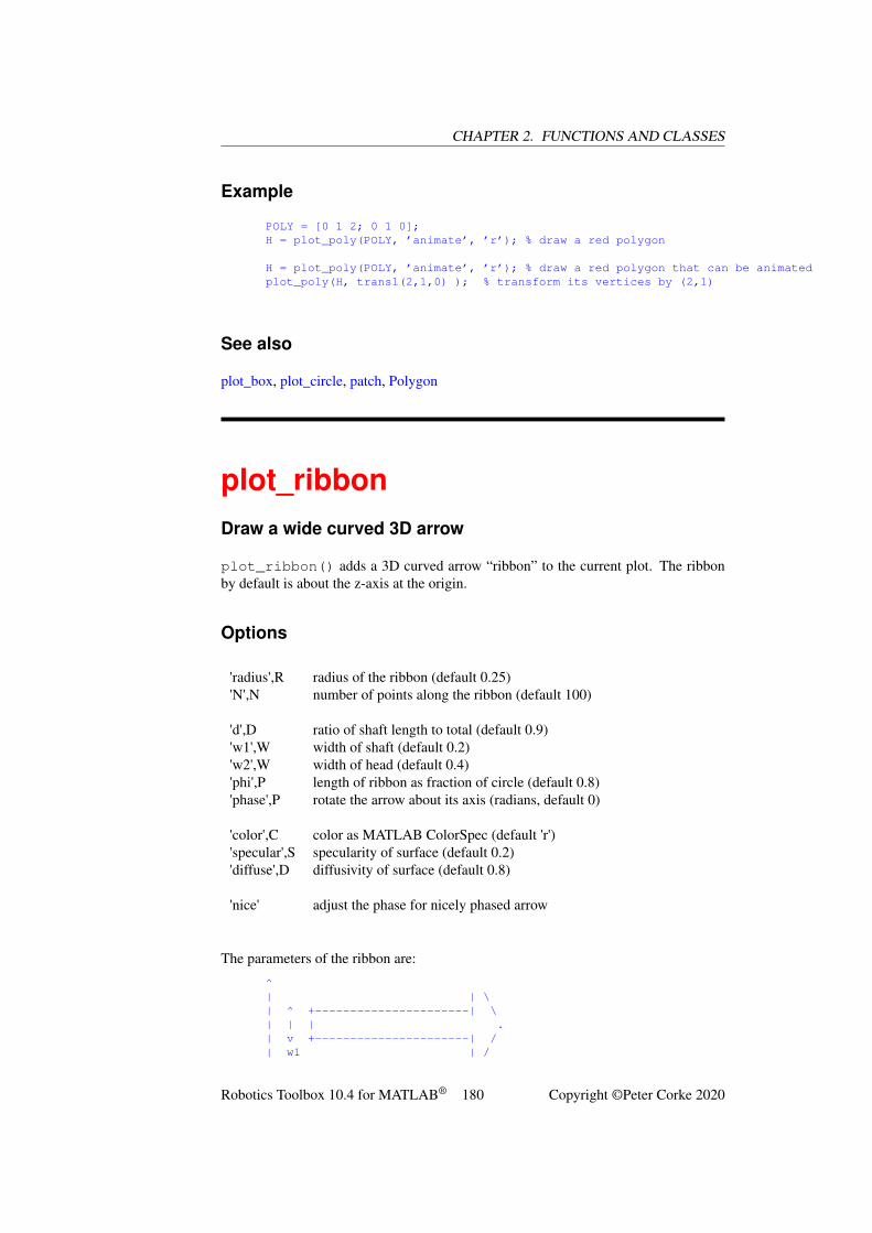
CHAPTER 2. FUNCTIONS AND CLASSES
Example
POLY = [0 1 2; 0 1 0];H = plot_poly(POLY, ’animate’, ’r’); % draw a red polygon
H = plot_poly(POLY, ’animate’, ’r’); % draw a red polygon that can be animatedplot_poly(H, transl(2,1,0) ); % transform its vertices by (2,1)
See also
plot_box, plot_circle, patch, Polygon
plot_ribbonDraw a wide curved 3D arrow
plot_ribbon() adds a 3D curved arrow “ribbon” to the current plot. The ribbonby default is about the z-axis at the origin.
Options
'radius',R radius of the ribbon (default 0.25)'N',N number of points along the ribbon (default 100)
'd',D ratio of shaft length to total (default 0.9)'w1',W width of shaft (default 0.2)'w2',W width of head (default 0.4)'phi',P length of ribbon as fraction of circle (default 0.8)'phase',P rotate the arrow about its axis (radians, default 0)
'color',C color as MATLAB ColorSpec (default 'r')'specular',S specularity of surface (default 0.2)'diffuse',D diffusivity of surface (default 0.8)
'nice' adjust the phase for nicely phased arrow
The parameters of the ribbon are:
^| | \| ^ +----------------------| \| | | .| v +----------------------| /| w1 | /
Robotics Toolbox 10.4 for MATLAB® 180 Copyright ©Peter Corke 2020
CHAPTER 2. FUNCTIONS AND CLASSES
v <---------- d --------->w2 <----------- phi ---------->
Examples
To draw the ribbon at distance A along the X, Y, Z axes is:
plot_ribbon2( SE3(A,0,0)*SE3.Ry(pi/2) )plot_ribbon2( SE3(0, A,0)*SE3.Rx(pi/2) )plot_ribbon2( SE3(0, 0, A) )shading interpcamlight
See also
plot_arrow, plot
plot_sphereDraw sphere
PLOT_SPHERE(C, R, LS) draws spheres in the current plot. C is the centre of thesphere (3×1), R is the radius and LS is an optional MATLAB ColorSpec, either a letteror a 3-vector.
PLOT_SPHERE(C, R, COLOR, ALPHA) as above but ALPHA specifies the opac-ity of the sphere where 0 is transparant and 1 is opaque. The default is 1.
If C (3×N) then N sphhere are drawn and H is N×1. If R (1×1) then all spheres havethe same radius or else R (1×N) to specify the radius of each sphere.
H = PLOT_SPHERE(...) as above but returns the handle(s) for the spheres.
Notes
• The sphere is always added, irrespective of figure hold state.
• The number of vertices to draw the sphere is hardwired.
Example
plot_sphere( mkgrid(2, 1), .2, ’b’); % Create four sphereslighting gouraud % full lighting modellight
Robotics Toolbox 10.4 for MATLAB® 181 Copyright ©Peter Corke 2020
CHAPTER 2. FUNCTIONS AND CLASSES
See also
: plot_point, plot_box, plot_circle, plot_ellipse, plot_poly
plotvolSet the bounds for a 2D or 3D plot
2D plots::
PLOTVOL([WX WY]) creates a new axis, and sets the bounds for a 2D plot, with Xspanning [-WX, WX] and Y spanning [-WY,WY].
PLOTVOL([XMIN XMAX YMIN YMAX]) as above but the X and Y axis limits areexplicitly provided.
3D plots::
PLOTVOL(W) creates a new axis, and sets the bounds for a 3D plot with X, Y and Zspanning the interval -W to W.
PLOTVOL([WX WY WZ]) as above with X spanning [-WX, WX], Y spanning [-WY,WY] and Z spanning [-WZ, WZ].
Notes
• The axes are labelled, grid is enabled, aspect ratio set to 1:1.
• Hold is enabled for subsequent plots.
See also
: axis
PluckerPlucker coordinate class
Concrete class to represent a 3D line using Plucker coordinates.
Robotics Toolbox 10.4 for MATLAB® 182 Copyright ©Peter Corke 2020
CHAPTER 2. FUNCTIONS AND CLASSES
Methods
Plucker Contructor from pointsPlucker.planes Constructor from planesPlucker.pointdir Constructor from point and direction
Information and test methods
closest closest point on linecommonperp common perpendicular for two linescontains test if point is on linedistance minimum distance between two linesintersects intersection point for two linesintersect_plane intersection points with a planeintersect_volume intersection points with a volumepp principal pointppd principal point distance from originpoint generate point on line
Conversion methods
char convert to human readable stringdouble convert to 6-vectorskew convert to 4×4 skew symmetric matrix
Display and print methods
display display in human readable formplot plot line
Operators
* multiply Plucker matrix by a general matrix| test if lines are parallel^ test if lines intersect== test if two lines are equivalent∼= test if lines are not equivalent
Notes
• This is reference (handle) class object
Robotics Toolbox 10.4 for MATLAB® 183 Copyright ©Peter Corke 2020
CHAPTER 2. FUNCTIONS AND CLASSES
• Plucker objects can be used in vectors and arrays
References
• Ken Shoemake, “Ray Tracing News”, Volume 11, Number 1 http://www.realtimerendering.com/resources/RTNews/html/rtnv11n1.html#art3
• Matt Mason lecture notes http://www.cs.cmu.edu/afs/cs/academic/class/16741-s07/www/lectures/lecture9.pdf
• Robotics, Vision & Control: Second Edition, P. Corke, Springer 2016; p596-7.
Implementation notes
• The internal representation is two 3-vectors: v (direction), w (moment).
• There is a huge variety of notation used across the literature, as well as the or-dering of the direction and moment components in the 6-vector.
Plucker.PluckerCreate Plucker line object
P = Plucker(P1, P2) create a Plucker object that represents the line joining the3D points P1 (3×1) and P2 (3×1). The direction is from P2 to P1.
P = Plucker(X) creates a Plucker object from X (6×1) = [V,W] where V (3×1)is the moment and W (3×1) is the line direction.
P = Plucker(L) creates a copy of the Plucker object L.
Plucker.charConvert to string
s = P.char() is a string showing Plucker parameters in a compact single lineformat.
See also
Plucker.display
Robotics Toolbox 10.4 for MATLAB® 184 Copyright ©Peter Corke 2020
CHAPTER 2. FUNCTIONS AND CLASSES
Plucker.closestPoint on line closest to given point
P = PL.closest(X) is the coordinate of a point (3×1) on the line that is closestto the point X (3×1).
[P,d] = PL.closest(X) as above but also returns the minimum distance be-tween the point and the line.
[P,dist,lambda] = PL.closest(X) as above but also returns the line pa-rameter lambda corresponding to the point on the line, ie. P = PL.point(lambda)
See also
Plucker.point
Plucker.commonperpCommon perpendicular to two lines
P = PL1.commonperp(PL2) is a Plucker object representing the common per-pendicular line between the lines represented by the Plucker objects PL1 and PL2.
See also
Plucker.intersect
Plucker.containsTest if point is on the line
PL.contains(X) is true if the point X (3×1) lies on the line defined by the Pluckerobject PL.
Plucker.displayDisplay parameters
P.display() displays the Plucker parameters in compact single line format.
Robotics Toolbox 10.4 for MATLAB® 185 Copyright ©Peter Corke 2020
CHAPTER 2. FUNCTIONS AND CLASSES
Notes
• This method is invoked implicitly at the command line when the result of anexpression is a Plucker object and the command has no trailing
• semicolon.
See also
Plucker.char
Plucker.distance
Distance between lines
d = P1.distance(P2) is the minimum distance between two lines representedby Plucker objects P1 and P2.
Notes
• Works for parallel, skew and intersecting lines.
Plucker.double
Convert Plucker coordinates to real vector
PL.double() is a vector (6×1) comprising the Plucker moment and direction vec-tors.
Plucker.eq
Test if two lines are equivalent
PL1 == PL2 is true if the Plucker objects describe the same line in space. Note thatbecause of the over parameterization, lines can be equivalent even if they have differentparameters.
Robotics Toolbox 10.4 for MATLAB® 186 Copyright ©Peter Corke 2020
CHAPTER 2. FUNCTIONS AND CLASSES
Plucker.get.uwLine direction as a unit vector
PL.UW is a unit-vector parallel to the line
Plucker.intersect_planeLine intersection with plane
X = PL.intersect_plane(PI) is the point where the Plucker line PL inter-sects the plane PI. X=[] if no intersection.
The plane PI can be either:
• a vector (1×4) = [a b c d] to describe the plane ax+by+cz+d=0.
• a structure with a normal PI.n (3×1) and an offset PI.p (1×1) such that PI.nX + PI.p = 0.
[X,lambda] = PL.intersect_plane(P) as above but also returns the lineparameter at the intersection point, ie. X = PL.point(lambda).
See also
Plucker.point
Plucker.intersect_volumeLine intersection with volume
P = PL.intersect_volume(BOUNDS) is a matrix (3×N) with columns that in-dicate where the Plcuker line PL intersects the faces of a volume specified by BOUNDS= [xmin xmax ymin ymax zmin zmax]. The number of columns N is either 0 (the lineis outside the plot volume) or 2 (where the line pierces the bounding volume).
[P,lambda] = PL.intersect_volume(bounds, line) as above but alsoreturns the line parameters (1×N) at the intersection points, ie. X = PL.point(lambda).
See also
Plucker.plot, Plucker.point
Robotics Toolbox 10.4 for MATLAB® 187 Copyright ©Peter Corke 2020
CHAPTER 2. FUNCTIONS AND CLASSES
Plucker.intersectsFind intersection of two lines
P = P1.intersects(P2) is the point of intersection (3× 1) of the lines repre-sented by Plucker objects P1 and P2. P = [] if the lines do not intersect, or the lines areequivalent.
Notes
• Can be used in operator form as P1P2.
• Returns [] if the lines are equivalent (P1==P2) since they would intersect at aninfinite number of points.
See also
Plucker.commonperp, Plucker.eq, Plucker.mpower
Plucker.isparallelTest if lines are parallel
P1.isparallel(P2) is true if the lines represented by Plucker objects P1 and P2are parallel.
See also
Plucker.or, Plucker.intersects
Plucker.mpowerTest if lines intersect
P1^P2 is true if lines represented by Plucker objects P1 and P2 intersect at a point.
Notes
• Is false if the lines are equivalent since they would intersect at an infinite numberof points.
Robotics Toolbox 10.4 for MATLAB® 188 Copyright ©Peter Corke 2020
CHAPTER 2. FUNCTIONS AND CLASSES
See also
Plucker.intersects, Plucker.parallel
Plucker.mtimesPlucker multiplication
PL1 * PL2 is the scalar reciprocal product.
PL * M is the product of the Plucker skew matrix and M (4×N).
M * PL is the product of M (N ×4) and the Plucker skew matrix (4×4).
Notes
• The * operator is overloaded for convenience.
• Multiplication or composition of Plucker lines is not defined.
• Premultiplying by an SE3 will transform the line with respect to the world coor-dinate frame.
See also
Plucker.skew, SE3.mtimes
Plucker.neTest if two lines are not equivalent
PL1 ̸= PL2 is true if the Plucker objects describe different lines in space. Note thatbecause of the over parameterization, lines can be equivalent even if they have differentparameters.
Plucker.orTest if lines are parallel
P1|P2 is true if the lines represented by Plucker objects P1 and P2 are parallel.
Robotics Toolbox 10.4 for MATLAB® 189 Copyright ©Peter Corke 2020
CHAPTER 2. FUNCTIONS AND CLASSES
Notes
• Can be used in operator form as P1|P2.
See also
Plucker.isparallel, Plucker.mpower
Plucker.planesCreate Plucker line from two planes
P = Plucker.planes(PI1, PI2) is a Plucker object that represents the lineformed by the intersection of two planes PI1, PI2 (each 4×1).
Notes
• Planes are given by the 4-vector [a b c d] to represent ax+by+cz+d=0.
Plucker.plotPlot a line
PL.plot(OPTIONS) adds the Plucker line PL to the current plot volume.
PL.plot(B, OPTIONS) as above but plots within the plot bounds B = [XMINXMAX YMIN YMAX ZMIN ZMAX].
Options
• Are passed directly to plot3, eg. 'k–', 'LineWidth', etc.
Notes
• If the line does not intersect the current plot volume nothing will be displayed.
See also
plot3, Plucker.intersect_volume
Robotics Toolbox 10.4 for MATLAB® 190 Copyright ©Peter Corke 2020
CHAPTER 2. FUNCTIONS AND CLASSES
Plucker.point
Generate point on line
P = PL.point(LAMBDA) is a point on the line, where LAMBDA is the parametricdistance along the line from the principal point of the line P = PP + PL.UW*LAMBDA.
See also
Plucker.pp, Plucker.closest
Plucker.pointdir
Construct Plucker line from point and direction
P = Plucker.pointdir(P, W) is a Plucker object that represents the line con-taining the point P (3×1) and parallel to the direction vector W (3×1).
See also
: Plucker
Plucker.pp
Principal point of the line
P = PL.pp() is the point on the line that is closest to the origin.
Notes
• Same as Plucker.point(0)
See also
Plucker.ppd, Plucker.point
Robotics Toolbox 10.4 for MATLAB® 191 Copyright ©Peter Corke 2020
CHAPTER 2. FUNCTIONS AND CLASSES
Plucker.ppdDistance from principal point to the origin
P = PL.ppd() is the distance from the principal point to the origin. This is thesmallest distance of any point on the line to the origin.
See also
Plucker.pp
Plucker.skewSkew matrix form of the line
L = PL.skew() is the Plucker matrix, a 4×4 skew-symmetric matrix representa-tion of the line.
Notes
• For two homogeneous points P and Q on the line, PQ'-QP'is also skew symmet-ric.
• The projection of Plucker line by a perspective camera is a homogeneous line(3×1) given by vex(C*L*C') where C (3×4) is the camera matrix.
QuaternionQuaternion class
A quaternion is 4-element mathematical object comprising a scalar s, and a vector vwhich can be considered as a pair (s,v). In the Toolbox it is denoted by q = s <<vx,vy, vz>>.
A quaternion of unit length can be used to represent 3D orientation and is implementedby the subclass UnitQuaternion.
Robotics Toolbox 10.4 for MATLAB® 192 Copyright ©Peter Corke 2020
CHAPTER 2. FUNCTIONS AND CLASSES
Constructors
Quaternion general constructorQuaternion.pure pure quaternion
Display and print methods
display print in human readable form
Group operations
* quaternion (Hamilton) product or elementwise multiplication by scalar/ multiply by inverse or elementwise division by scalar^ exponentiate (integer only)+ elementwise sum of quaternion elements- elementwise difference of quaternion elementsconj conjugateexp exponentiallog logarithminv inverseprod product of elementsunit unitized quaternion
Methods
inner inner productisequal test for non-equalitynorm norm, or length
Conversion methods
char convert to stringdouble quaternion elements as 4-vectormatrix quaternion as a 4×4 matrix
Overloaded operators
== test for quaternion equality∼= test for quaternion inequality
Robotics Toolbox 10.4 for MATLAB® 193 Copyright ©Peter Corke 2020
CHAPTER 2. FUNCTIONS AND CLASSES
Properties (read only)
s real partv vector part
Notes
• This is reference (handle) class object
• Quaternion objects can be used in vectors and arrays.
References
• Animating rotation with quaternion curves, K. Shoemake, in Proceedings ofACM SIGGRAPH, (San Fran cisco), pp. 245-254, 1985.
• On homogeneous transforms, quaternions, and computational efficiency, J. Funda,R. Taylor, and R. Paul,
• IEEE Transactions on Robotics and Automation, vol. 6, pp. 382-388, June 1990.
• Quaternions for Computer Graphics, J. Vince, Springer 2011.
• Robotics, Vision & Control: Second Edition, P. Corke, Springer 2016; p44-45.
See also
UnitQuaternion
Quaternion.QuaternionConstruct a quaternion object
Q = Quaternion(S, V) is a Quaternion formed from the scalar S and vectorpart V (1×3).
Q = Quaternion([S V1 V2 V3]) is a Quaternion formed by specifying di-rectly its 4 elements.
Q = Quaternion() is a zero Quaternion, all its elements are zero.
Notes
• The constructor is not vectorized, it cannot create a vector of Quaternions.
Robotics Toolbox 10.4 for MATLAB® 194 Copyright ©Peter Corke 2020
CHAPTER 2. FUNCTIONS AND CLASSES
Quaternion.char
Convert to string
S = Q.char() is a compact string representation of the Quaternion's value as a4-tuple. If Q is a vector then S has one line per element.
Notes
• The vector part is delimited by double angle brackets, to differentiate from aUnitQuaternion which is delimited by single angle brackets.
See also
UnitQuaternion.char
Quaternion.conj
Conjugate of a quaternion
Q.conj() is a Quaternion object representing the conjugate of Q.
Notes
• Conjugatation is the negation of the vector component.
See also
Quaternion.inv
Quaternion.display
Display quaternion
Q.display() displays a compact string representation of the Quaternion's value asa 4-tuple. If Q is a vector then S has one line per element.
Robotics Toolbox 10.4 for MATLAB® 195 Copyright ©Peter Corke 2020
CHAPTER 2. FUNCTIONS AND CLASSES
Notes
• This method is invoked implicitly at the command line when the result of anexpression is a Quaternion object and the command has no trailing
• semicolon.
• The vector part is displayed with double brackets << 1, 0, 0 >> to distinguishit from a UnitQuaternion which displays as < 1, 0, 0 >
• If Q is a vector of Quaternion objects the elements are displayed on consecutivelines.
See also
Quaternion.char
Quaternion.doubleConvert a quaternion to a 4-element vector
V = Q.double() is a row vector (1 × 4) comprising the Quaternion elements,scalar then vector, ie. V = [s vx vy vz]. If Q is a vector (1×N) of Quaternion ob-jects then V is a matrix (N ×4) with rows corresponding to the quaternion elements.
Quaternion.eqTest quaternion equality
Q1 == Q2 is true if the Quaternions Q1 and Q2 are equal.
Notes
• Overloaded operator '=='.
• Equality means elementwise equality of Quaternion elements.
• If either, or both, of Q1 or Q2 are vectors, then the result is a vector.
– if Q1 is a vector (1×N) then R is a vector (1×N) such that R(i) = Q1(i)==Q2.
– if Q2 is a vector (1×N) then R is a vector (1×N) such that R(i) = Q1==Q2(i).
– if both Q1 and Q2 are vectors (1×N) then R is a vector (1×N) such thatR(i) = Q1(i)==Q2(i).
Robotics Toolbox 10.4 for MATLAB® 196 Copyright ©Peter Corke 2020
CHAPTER 2. FUNCTIONS AND CLASSES
See also
Quaternion.ne
Quaternion.expExponential of quaternion
Q.log() is the logarithm of the Quaternion Q.
See also
Quaternion.exp
Quaternion.innerQuaternion inner product
V = Q1.inner(Q2) is the inner (dot) product of two vectors (1× 4), comprisingthe elements of Q1 and Q2 respectively.
Notes
• Q1.inner(Q1) is the same as Q1.norm().
See also
Quaternion.norm
Quaternion.invInvert a quaternion
Q.inv() is a Quaternion object representing the inverse of Q.
Notes
• If Q is a vector then an equal length vector of Quaternion objects is computedrepresenting the elementwise inverse of Q.
Robotics Toolbox 10.4 for MATLAB® 197 Copyright ©Peter Corke 2020
CHAPTER 2. FUNCTIONS AND CLASSES
See also
Quaternion.conj
Quaternion.isequalTest quaternion element equality
ISEQUAL(Q1,Q2) is true if the Quaternions Q1 and Q2 are equal.
Notes
• Used by test suite verifyEqual() in addition to eq().
• Invokes eq() so respects double mapping for UnitQuaternion.
See also
Quaternion.eq
Quaternion.logLogarithm of quaternion
Q.log() is the logarithm of the Quaternion Q.
See also
Quaternion.exp
Quaternion.matrixMatrix representation of Quaternion
Q.matrix() is a matrix (4×4) representation of the Quaternion Q.
Quaternion, or Hamilton, multiplication can be implemented as a matrix-vector prod-uct, where the column-vector is the elements of a second quaternion:
matrix(Q1) * double(Q2)’
Robotics Toolbox 10.4 for MATLAB® 198 Copyright ©Peter Corke 2020
CHAPTER 2. FUNCTIONS AND CLASSES
Notes
• This matrix is not unique, other matrices will serve the purpose for multiplica-tion, see https://en.wikipedia.org/wiki/Quaternion#Matrix_representations
• The determinant of the matrix is the norm of the Quaternion to the fourth power.
See also
Quaternion.double, Quaternion.mtimes
Quaternion.minusSubtract quaternions
Q1-Q2 is a Quaternion formed from the element-wise difference of Quaternion ele-ments.
Q1-V is a Quaternion formed from the element-wise difference of Q1 and the vectorV (1×4).
Notes
• Overloaded operator '-'.
• Effectively V is promoted to a Quaternion.
See also
Quaternion.plus
Quaternion.mpowerRaise quaternion to integer power
Q^N is the Quaternion Q raised to the integer power N.
Notes
• Overloaded operator '^textquotesingle .
• N must be an integer, computed by repeated multiplication.
Robotics Toolbox 10.4 for MATLAB® 199 Copyright ©Peter Corke 2020
CHAPTER 2. FUNCTIONS AND CLASSES
See also
Quaternion.mtimes
Quaternion.mrdivideQuaternion quotient.
R = Q1/Q2 is a Quaternion formed by Hamilton product of Q1 and inv(Q2).R = Q/S is the element-wise division of Quaternion elements by the scalar S.
Notes
• Overloaded operator '/'.
• If either, or both, of Q1 or Q2 are vectors, then the result is a vector.
– if Q1 is a vector (1×N) then R is a vector (1×N) such that R(i) = Q1(i)./Q2.
– if Q2 is a vector (1×N) then R is a vector (1×N) such that R(i) = Q1./Q2(i).
– if both Q1 and Q2 are vectors (1×N) then R is a vector (1×N) such thatR(i) = Q1(i)./Q2(i).
See also
Quaternion.mtimes, Quaternion.mpower, Quaternion.plus, Quaternion.minus
Quaternion.mtimesMultiply a quaternion object
Q1*Q2 is a Quaternion formed by the Hamilton product of two Quaternions.Q*S is the element-wise multiplication of Quaternion elements by the scalar S.S*Q is the element-wise multiplication of Quaternion elements by the scalar S.
Notes
• Overloaded operator '*'.
• If either, or both, of Q1 or Q2 are vectors, then the result is a vector.
– if Q1 is a vector (1×N) then R is a vector (1×N) such that R(i) = Q1(i)*Q2.
Robotics Toolbox 10.4 for MATLAB® 200 Copyright ©Peter Corke 2020
CHAPTER 2. FUNCTIONS AND CLASSES
– if Q2 is a vector (1×N) then R is a vector (1×N) such that R(i) = Q1*Q2(i).
– if both Q1 and Q2 are vectors (1×N) then R is a vector (1×N) such thatR(i) = Q1(i)*Q2(i).
See also
Quaternion.mrdivide, Quaternion.mpower
Quaternion.neTest quaternion inequality
Q1 ̸= Q2 is true if the Quaternions Q1 and Q2 are not equal.
Notes
• Overloaded operator '̸='.
• If either, or both, of Q1 or Q2 are vectors, then the result is a vector.
– if Q1 is a vector (1×N) then R is a vector (1×N) such that R(i) = Q1(i)̸=Q2.
– if Q2 is a vector (1×N) then R is a vector (1×N) such that R(i) = Q1̸=Q2(i).
– if both Q1 and Q2 are vectors (1×N) then R is a vector (1×N) such thatR(i) = Q1(i)̸=Q2(i).
See also
Quaternion.eq
Quaternion.newConstruct a new quaternion
QN = Q.new() constructs a new Quaternion object.
QN = Q.new([S, V1, V2, V3]) as above but specified directly by its 4 ele-ments.
QN = Q.new(S, V) as above but specified directly by the scalar S and vector partV (1×3)
Robotics Toolbox 10.4 for MATLAB® 201 Copyright ©Peter Corke 2020
CHAPTER 2. FUNCTIONS AND CLASSES
Notes
• Polymorphic with UnitQuaternion and RTBPose derived classes.
Quaternion.normQuaternion magnitude
Q.norm(Q) is the scalar norm or magnitude of the Quaternion Q.
Notes
• This is the Euclidean norm of the Quaternion written as a 4-vector.
• A unit-quaternion has a norm of one and is represented by the UnitQuaternionclass.
See also
Quaternion.inner, Quaternion.unit, UnitQuaternion
Quaternion.plusAdd quaternions
Q1+Q2 is a Quaternion formed from the element-wise sum of Quaternion elements.
Q1+V is a Quaternion formed from the element-wise sum of Q1 and the vector V(1×4).
Notes
• Overloaded operator '+'.
• Effectively V is promoted to a Quaternion.
See also
Quaternion.minus
Robotics Toolbox 10.4 for MATLAB® 202 Copyright ©Peter Corke 2020
CHAPTER 2. FUNCTIONS AND CLASSES
Quaternion.prodProduct of quaternions
prod(Q) is the product of the elements of the vector of Quaternion objects Q.
See also
Quaternion.mtimes, RTBPose.prod
Quaternion.pureConstruct a pure quaternion
Q = Quaternion.pure(V) is a pure Quaternion formed from the vector V (1×3) and has a zero scalar part.
Quaternion.set.sSet scalar component
Q.s = S sets the scalar part of the Quaternion object to S.
Quaternion.set.vSet vector component
Q.v = V sets the vector part of the Quaternion object to V (1×3).
Quaternion.unitUnitize a quaternion
QU = Q.unit() is a Quaternion with a norm of 1. If Q is a vector (1×N) then QUis also a vector (1×N).
Robotics Toolbox 10.4 for MATLAB® 203 Copyright ©Peter Corke 2020
CHAPTER 2. FUNCTIONS AND CLASSES
Notes
• This is Quaternion of unit norm, not a UnitQuaternion object.
See also
Quaternion.norm, UnitQuaternion
r2tConvert rotation matrix to a homogeneous transform
T = R2T(R) is an SE(2) or SE(3) homogeneous transform equivalent to an SO(2)or SO(3) orthonormal rotation matrix R with a zero translational component. Worksfor T in either SE(2) or SE(3):
• if R is 2×2 then T is 3×3, or
• if R is 3×3 then T is 4×4.
Notes
• Translational component is zero.
• For a rotation matrix sequence (K ×K ×N) returns a homogeneous transformsequence (K +1×K+1×N).
See also
t2r
randinitReset random number generator
RANDINIT resets the defaul random number stream. For example:
Robotics Toolbox 10.4 for MATLAB® 204 Copyright ©Peter Corke 2020
CHAPTER 2. FUNCTIONS AND CLASSES
>> randans =
0.8147>> randans =
0.9058>> randans =
0.1270>> randinit>> randans =
0.8147
rot2SO(2) rotation matrix
R = ROT2(THETA) is an SO(2) rotation matrix (2× 2) representing a rotation ofTHETA radians.
R = ROT2(THETA, ’deg’) as above but THETA is in degrees.
See also
trot2, isrot2, trplot2, rotx, roty, rotz, SO2
rotxSO(3) rotation about X axis
R = ROTX(THETA) is an SO(3) rotation matrix (3× 3) representing a rotation ofTHETA radians about the x-axis.
R = ROTX(THETA, ’deg’) as above but THETA is in degrees.
See also
trotx, roty, rotz, angvec2r, rot2, SO3.Rx
Robotics Toolbox 10.4 for MATLAB® 205 Copyright ©Peter Corke 2020
CHAPTER 2. FUNCTIONS AND CLASSES
rotySO(3) rotation about Y axis
R = ROTY(THETA) is an SO(3) rotation matrix (3× 3) representing a rotation ofTHETA radians about the y-axis.
R = ROTY(THETA, ’deg’) as above but THETA is in degrees.
See also
troty, rotx, rotz, angvec2r, rot2, SO3.Ry
rotzSO(3) rotation about Z axis
R = ROTZ(THETA) is an SO(3) rotation matrix (3× 3) representing a rotation ofTHETA radians about the z-axis.
R = ROTZ(THETA, ’deg’) as above but THETA is in degrees.
See also
trotz, rotx, roty, angvec2r, rot2, SO3.Rx
rpy2jacJacobian from RPY angle rates to angular velocity
J = RPY2JAC(RPY, OPTIONS) is a Jacobian matrix (3×3) that maps ZYX roll-pitch-yaw angle rates to angular velocity at the operating point RPY=[R,P,Y].
J = RPY2JAC(R, P, Y, OPTIONS) as above but the roll-pitch-yaw angles arepassed as separate arguments.
Options
Robotics Toolbox 10.4 for MATLAB® 206 Copyright ©Peter Corke 2020
CHAPTER 2. FUNCTIONS AND CLASSES
'xyz' Use XYZ roll-pitch-yaw angles'yxz' Use YXZ roll-pitch-yaw angles
Notes
• Used in the creation of an analytical Jacobian.
• Angles in radians, rates in radians/sec.
Reference
• Robotics, Vision & Control: Second Edition, P. Corke, Springer 2016; p232-3.
See also
eul2jac, rpy2r, SerialLink.jacobe
rpy2rRoll-pitch-yaw angles to SO(3) rotation matrix
R = RPY2R(ROLL, PITCH, YAW, OPTIONS) is an SO(3) orthonornal rotationmatrix (3× 3) equivalent to the specified roll, pitch, yaw angles angles. These corre-spond to rotations about the Z, Y, X axes respectively. If ROLL, PITCH, YAW arecolumn vectors (N×1) then they are assumed to represent a trajectory and R is a three-dimensional matrix (3× 3×N), where the last index corresponds to rows of ROLL,PITCH, YAW.
R = RPY2R(RPY, OPTIONS) as above but the roll, pitch, yaw angles are takenfrom the vector (1× 3) RPY=[ROLL,PITCH,YAW]. If RPY is a matrix (N × 3) then Ris a three-dimensional matrix (3×3×N), where the last index corresponds to rows ofRPY which are assumed to be [ROLL,PITCH,YAW].
Options
'deg' Compute angles in degrees (radians default)'xyz' Rotations about X, Y, Z axes (for a robot gripper)'zyx' Rotations about Z, Y, X axes (for a mobile robot, default)'yxz' Rotations about Y, X, Z axes (for a camera)'arm' Rotations about X, Y, Z axes (for a robot arm)
Robotics Toolbox 10.4 for MATLAB® 207 Copyright ©Peter Corke 2020
CHAPTER 2. FUNCTIONS AND CLASSES
'vehicle'Rotations about Z, Y, X axes (for a mobile robot)
'camera' Rotations about Y, X, Z axes (for a camera)
Note
• Toolbox rel 8-9 has XYZ angle sequence as default.
• ZYX order is appropriate for vehicles with direction of travel in the X direction.XYZ order is appropriate if direction of travel is in the Z
• direction.
• 'arm', 'vehicle', 'camera'are synonyms for 'xyz', 'zyx'and 'yxz'respectively.
See also
tr2rpy, eul2tr
rpy2trRoll-pitch-yaw angles to SE(3) homogeneous transform
T = RPY2TR(ROLL, PITCH, YAW, OPTIONS) is an SE(3) homogeneous trans-formation matrix (4× 4) with zero translation and rotation equivalent to the specifiedroll, pitch, yaw angles angles. These correspond to rotations about the Z, Y, X axesrespectively. If ROLL, PITCH, YAW are column vectors (N ×1) then they are assumedto represent a trajectory and R is a three-dimensional matrix (4×4×N), where the lastindex corresponds to rows of ROLL, PITCH, YAW.
T = RPY2TR(RPY, OPTIONS) as above but the roll, pitch, yaw angles are takenfrom the vector (1× 3) RPY=[ROLL,PITCH,YAW]. If RPY is a matrix (N × 3) then Ris a three-dimensional matrix (4×4×N), where the last index corresponds to rows ofRPY which are assumed to be ROLL,PITCH,YAW].
Options
'deg' Compute angles in degrees (radians default)'xyz' Rotations about X, Y, Z axes (for a robot gripper)'zyx' Rotations about Z, Y, X axes (for a mobile robot, default)'yxz' Rotations about Y, X, Z axes (for a camera)'arm' Rotations about X, Y, Z axes (for a robot arm)
Robotics Toolbox 10.4 for MATLAB® 208 Copyright ©Peter Corke 2020
CHAPTER 2. FUNCTIONS AND CLASSES
'vehicle'Rotations about Z, Y, X axes (for a mobile robot)
'camera' Rotations about Y, X, Z axes (for a camera)
Note
• Toolbox rel 8-9 has the reverse angle sequence as default.
• ZYX order is appropriate for vehicles with direction of travel in the X direction.XYZ order is appropriate if direction of travel is in the Z
• direction.
• 'arm', 'vehicle', 'camera'are synonyms for 'xyz', 'zyx'and 'yxz'respectively.
See also
tr2rpy, rpy2r, eul2tr
rt2trConvert rotation and translation to homogeneous transform
TR = RT2TR(R, t) is a homogeneous transformation matrix (N+1×N+1) formedfrom an orthonormal rotation matrix R (N ×N) and a translation vector t (N × 1).Works for R in SO(2) or SO(3):
• If R is 2×2 and t is 2×1, then TR is 3×3
• If R is 3×3 and t is 3×1, then TR is 4×4
For a sequence R (N ×N ×K) and t (N ×K) results in a transform sequence (N +1×N+1×K).
Notes
• The validity of R is not checked
See also
t2r, r2t, tr2rt
Robotics Toolbox 10.4 for MATLAB® 209 Copyright ©Peter Corke 2020
CHAPTER 2. FUNCTIONS AND CLASSES
RTBPoseSuperclass for SO2, SO3, SE2, SE3
This abstract class provides common methods for the 2D and 3D orientation and poseclasses: SO2, SE2, SO3 and SE3.
Display and print methods
animate graphically animate coordinate frame for posedisplay print the pose in human readable matrix formplot graphically display coordinate frame for poseprint print the pose in single line format
Group operations
* mtimes: multiplication within group, also transform vector/ mrdivide: multiplication within group by inverseprod mower: product of elements
Methods
dim dimension of the underlying matrixisSE true for SE2 and SE3issym true if value is symbolicsimplify apply symbolic simplification to all elementsvpa apply vpa to all elements
% Conversion methods::
char convert to human readable matrix as a stringdouble convert to real rotation or homogeneous transformation matrix
Operators
+ plus: elementwise addition, result is a matrix- minus: elementwise subtraction, result is a matrix== eq: test equality∼= ne: test inequality
Robotics Toolbox 10.4 for MATLAB® 210 Copyright ©Peter Corke 2020
CHAPTER 2. FUNCTIONS AND CLASSES
Compatibility methods
A number of compatibility methods give the same behaviour as the classic RTB func-tions:
tr2rt convert to rotation matrix and translation vectort2r convert to rotation matrixtranimate animate coordinate frametrprint print single line representationtrprint2 print single line representationtrplot plot coordinate frametrplot2 plot coordinate frame
Notes
• This is a handle class.
• RTBPose subclasses can be used in vectors and arrays.
• Multiplication and division with normalization operations are performed in thesubclasses.
• SO3 is polymorphic with UnitQuaternion making it easy to change rotationalrepresentations.
See also
SO2, SO3, SE2, SE3
RTBPose.animateAnimate a coordinate frame
RTBPose.animate(P1, P2, OPTIONS) animates a 3D coordinate frame mov-ing from RTBPose P1 to RTBPose P2.
RTBPose.animate(P, OPTIONS) animates a coordinate frame moving from theidentity pose to the RTBPose P.
RTBPose.animate(PV, OPTIONS) animates a trajectory, where PV is a vectorof RTBPose subclass objects.
%
Options
Robotics Toolbox 10.4 for MATLAB® 211 Copyright ©Peter Corke 2020
CHAPTER 2. FUNCTIONS AND CLASSES
'fps', fps Number of frames per second to display (default 10)'nsteps', n The number of steps along the path (default 50)'axis',A Axis bounds [xmin, xmax, ymin, ymax, zmin, zmax]'movie',M Save frames as files in the folder M'cleanup' Remove the frame at end of animation'noxyz' Don't label the axes'rgb' Color the axes in the order x=red, y=green, z=blue'retain' Retain frames, don't animate
Additional options are passed through to tranimate or tranimate2.
See also
tranimate, tranimate2
RTBPose.charConvert to string
s = P.char() is a string showing RTBPose matrix elements as a matrix.
See also
RTBPose.display
RTBPose.dimDimension
N = P.dim() is the dimension of the matrix representing the RTBPose subclassinstance P. It is 2 for SO2, 3 for SE2 and SO3, and 4 for SE3.
RTBPose.displayDisplay pose in matrix form
P.display() displays the matrix elements for the RTBPose instance P to the con-sole. If P is a vector (1×N) then matrices are displayed sequentially.
Robotics Toolbox 10.4 for MATLAB® 212 Copyright ©Peter Corke 2020
CHAPTER 2. FUNCTIONS AND CLASSES
Notes
• This method is invoked implicitly at the command line when the result of anexpression is an RTBPose subclass object and the command has no trailing
• semicolon.
• If the function cprintf is found is used to colorise the matrix: rotational elementsin red, translational in blue.
• See https://www.mathworks.com/matlabcentral/fileexchange/24093-cprintf-display-formatted-colored-text-in-the-command-window
See also
SO2, SO3, SE2, SE3
RTBPose.double
Convert to matrix
T = P.double() is a native matrix representation of the RTBPose subclass in-stance P, either a rotation matrix or a homogeneous transformation matrix.
If P is a vector (1×N) then T will be a 3-dimensional array (M×M×N).
Notes
• If the pose is symbolic the result will be a symbolic matrix.
RTBPose.ishomog
Test if SE3 class (compatibility)
ISHOMOG(T) is true (1) if T is of class SE3.
See also
ishomog
Robotics Toolbox 10.4 for MATLAB® 213 Copyright ©Peter Corke 2020
CHAPTER 2. FUNCTIONS AND CLASSES
RTBPose.ishomog2Test if SE2 class (compatibility)
ISHOMOG2(T) is true (1) if T is of class SE2.
See also
ishomog2
RTBPose.isrotTest if SO3 class (compatibility)
ISROT(R) is true (1) if R is of class SO3.
See also
isrot
RTBPose.isrot2Test if SO2 class (compatibility)
ISROT2(R) is true (1) if R is of class SO2.
See also
isrot2
RTBPose.isSETest if rigid-body motion
P.isSE() is true if P is an instance of the RTBPose sublass SE2 or SE3.
Robotics Toolbox 10.4 for MATLAB® 214 Copyright ©Peter Corke 2020
CHAPTER 2. FUNCTIONS AND CLASSES
RTBPose.issymTest if pose is symbolic
P.issym() is true if the RTBPose subclass instance P has symbolic rather than realvalues.
RTBPose.isvecTest if vector (compatibility)
ISVEC(T) is always false.
See also
isvec
RTBPose.minusSubtract poses
P1-P2 is the elementwise difference of the matrix elements of the two poses. Theresult is a matrix not the input class type since the result of subtraction is not in thegroup.
RTBPose.mpowerExponential of pose
P^N is an RTBPose subclass instance equal to RTBPose subclass instance P raised tothe integer power N. It is equivalent of compounding P with itself N-1 times.
Notes
• N can be 0 in which case the result is the identity element.
• N can be negative which is equivalent to the inverse of ^-N).
Robotics Toolbox 10.4 for MATLAB® 215 Copyright ©Peter Corke 2020
CHAPTER 2. FUNCTIONS AND CLASSES
See also
RTBPose.power, RTBPose.mtimes, RTBPose.times
RTBPose.mrdivideCompound SO2 object with inverse
R = P/Q is an RTBPose subclass instance representing the composition of the RTB-Pose subclass instance P by the inverse of the RTBPose subclass instance Q.
If either, or both, of P or Q are vectors, then the result is a vector.
• if P is a vector (1×N) then R is a vector (1×N) such that R(i) = P(i)/Q.
• if P is a vector (1×N) then R is a vector (1×N) such that R(i) = P/Q(i).
• if both P and Q are vectors (1×N) then R is a vector (1×N) such that R(i) =P(i)/Q(i).
Notes
• Computed by matrix multiplication of their equivalent matrices with the secondone inverted.
See also
RTBPose.mtimes
RTBPose.mtimesCompound pose objects
R = P*Q is an RTBPose subclass instance representing the composition of the RTB-Pose subclass instance P by the RTBPose subclass instance Q.
If either, or both, of P or Q are vectors, then the result is a vector.
• if P is a vector (1×N) then R is a vector (1×N) such that R(i) = P(i)*Q.
• if P is a vector (1×N) then R is a vector (1×N) such that R(i) = P*Q(i).
• if both P and Q are vectors (1×N) then R is a vector (1×N) such that R(i) =P(i)*Q(i).
Robotics Toolbox 10.4 for MATLAB® 216 Copyright ©Peter Corke 2020
CHAPTER 2. FUNCTIONS AND CLASSES
W = P*V is a column vector (2×1) which is the transformation of the column vectorV (2×1) by the matrix representation of the RTBPose subclass instance P.
P can be a vector and/or V can be a matrix, a columnwise set of vectors:
• if P is a vector (1×N) then W is a matrix (2×N) such that W(:,i) = P(i)*V.
• if V is a matrix (2×N) V is a matrix (2×N) then W is a matrix (2×N) such thatW(:,i) = P*V(:,i).
• if P is a vector (1×N) and V is a matrix (2×N) then W is a matrix (2×N) suchthat W(:,i) = P(i)*V(:,i).
Notes
• Computed by matrix multiplication of their equivalent matrices.
See also
RTBPose.mrdivide
RTBPose.plotDraw a coordinate frame (compatibility)
trplot(P, OPTIONS) draws a 3D coordinate frame represented by P which isSO2, SO3, SE2 or SE3.
Compatible with matrix function trplot(T).
Options are passed through to trplot or trplot2 depending on the object type.
See also
trplot, trplot2
RTBPose.plusAdd poses
P1+P2 is the elementwise summation of the matrix elements of the RTBPose subclassinstances P1 and P2. The result is a native matrix not the input class type since theresult of addition is not in the group.
Robotics Toolbox 10.4 for MATLAB® 217 Copyright ©Peter Corke 2020
CHAPTER 2. FUNCTIONS AND CLASSES
RTBPose.power
Exponential of pose
P.^N is the exponential of P where N is an integer, followed by normalization. It isequivalent of compounding the rigid-body motion of P with itself N-1 times.
Notes
• N can be 0 in which case the result is the identity matrix.
• N can be negative which is equivalent to the inverse of P.abs(N).
See also
RTBPose.mpower, RTBPose.mtimes, RTBPose.times
RTBPose.print
Compact display of pose
P.print(OPTIONS) displays the RTBPose subclass instance P in a compact single-line format. If P is a vector then each element is printed on a separate line.
Example
T = SE3.rand()T.print(’rpy’, ’xyz’) % display using XYZ RPY angles
Notes
• Options are passed through to trprint or trprint2 depending on the object type.
See also
trprint, trprint2
Robotics Toolbox 10.4 for MATLAB® 218 Copyright ©Peter Corke 2020
CHAPTER 2. FUNCTIONS AND CLASSES
RTBPose.prod
Compound array of poses
P.prod() is an RTBPose subclass instance representing the product (composition)of the successive elements of P (1×N).
Note
• Composition is performed with the .* operator, ie. the product is renormalizedat every step.
See also
RTBPose.times
RTBPose.simplify
Symbolic simplification
P2 = P.simplify() applies symbolic simplification to each element of internalmatrix representation of the RTBPose subclass instance P.
See also
simplify
RTBPose.subs
Symbolic substitution
T = subs(T, old, new) replaces oldwith new in the symbolic transformationT.
See also: subs
Robotics Toolbox 10.4 for MATLAB® 219 Copyright ©Peter Corke 2020
CHAPTER 2. FUNCTIONS AND CLASSES
RTBPose.t2rGet rotation matrix (compatibility)
t2r(P) is a native matrix corresponding to the rotational component of the SE2 orSE3 instance P.
See also
t2r
RTBPose.tr2rtSplit rotational and translational components (compatibility)
[R,t] = tr2rt(P) is the rotation matrix and translation vector corresponding tothe SE2 or SE3 instance P.
See also
tr2rt
RTBPose.tranimateAnimate a 3D coordinate frame (compatibility)
TRANIMATE(P1, P2, OPTIONS) animates a 3D coordinate frame moving be-tween RTBPose subclass instances P1 and pose P2.
TRANIMATE(P, OPTIONS) animates a 2D coordinate frame moving from the iden-tity pose to the RTBPose subclass instance P.
TRANIMATE(PV, OPTIONS) animates a trajectory, where PV is a vector of RTB-Pose subclass instances.
Notes
• see tranimate for details of options.
• P, P1, P2, PV can be instances of SO3 or SE3.
Robotics Toolbox 10.4 for MATLAB® 220 Copyright ©Peter Corke 2020
CHAPTER 2. FUNCTIONS AND CLASSES
See also
RTBPose.animate, tranimate
RTBPose.tranimate2Animate a 2D coordinate frame (compatibility)
TRANIMATE2(P1, P2, OPTIONS) animates a 2D coordinate frame moving be-tween RTBPose subclass instances P1 and pose P2.
TRANIMATE2(P, OPTIONS) animates a 2D coordinate frame moving from theidentity pose to the RTBPose subclass instance P.
TRANIMATE2(PV, OPTIONS) animates a trajectory, where PV is a vector of RTB-Pose subclass instances.
Notes
• see tranimate2 for details of options.
• P, P1, P2, PV can be instances of SO2 or SE2.
See also
RTBPose.animate, tranimate
RTBPose.trplotDraw a 3D coordinate frame (compatibility)
trplot(P, OPTIONS) draws a 3D coordinate frame represented by RTBPose sub-class instance P.
Notes
• see trplot for details of options.
• P can be instances of SO3 or SE3.
See also
RTBPose.plot, trplot
Robotics Toolbox 10.4 for MATLAB® 221 Copyright ©Peter Corke 2020
CHAPTER 2. FUNCTIONS AND CLASSES
RTBPose.trplot2Draw a 2D coordinate frame (compatibility)
trplot2(P, OPTIONS) draws a 2D coordinate frame represented by RTBPosesubclass instance P.
Notes
• see trplot for details of options.
• P can be instances of SO2 or SE2.
See also
RTBPose.plot, trplot2
RTBPose.trprintCompact display of 3D rotation or transform (compatibility)
trprint(P, OPTIONS) displays the RTBPose subclass instance P in a compactsingle-line format. If P is a vector then each element is printed on a separate line.
Notes
• see trprint for details of options.
• P can be instances of SO3 or SE3.
See also
RTBPose.print, trprint
RTBPose.trprint2Compact display of 2D rotation or transform (compatibility)
trprint2(P, OPTIONS) displays the RTBPose subclass instance P in a compactsingle-line format. If P is a vector then each element is printed on a separate line.
Robotics Toolbox 10.4 for MATLAB® 222 Copyright ©Peter Corke 2020
CHAPTER 2. FUNCTIONS AND CLASSES
Notes
• see trprint for details of options.
• P can be instances of SO2 or SE2.
See also
RTBPose.print, trprint2
RTBPose.vpaVariable precision arithmetic
P2 = P.vpa() numerically evaluates each element of internal matrix representationof the RTBPose subclass instance P.
P2 = P.vpa(D) as above but with D decimal digit accuracy.
Notes
• Values of symbolic variables are taken from the workspace.
See also
vpa, simplify
SE2Representation of 2D rigid-body motion
This subclasss of RTBPose is an object that represents rigid-body motion in 2D. Inter-nally this is a 3×3 homogeneous transformation matrix (3×3) belonging to the groupSE(2).
Robotics Toolbox 10.4 for MATLAB® 223 Copyright ©Peter Corke 2020
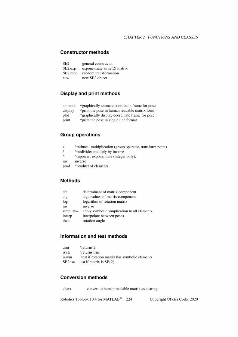
CHAPTER 2. FUNCTIONS AND CLASSES
Constructor methods
SE2 general constructorSE2.exp exponentiate an se(2) matrixSE2.rand random transformationnew new SE2 object
Display and print methods
animate ^graphically animate coordinate frame for posedisplay ^print the pose in human readable matrix formplot ^graphically display coordinate frame for poseprint ^print the pose in single line format
Group operations
* ^mtimes: multiplication (group operator, transform point)/ ^mrdivide: multiply by inverse^ ^mpower: exponentiate (integer only):inv inverseprod ^product of elements
Methods
det determinant of matrix componenteig eigenvalues of matrix componentlog logarithm of rotation matrixinv inversesimplify* apply symbolic simplication to all elementsinterp interpolate between posestheta rotation angle
Information and test methods
dim ^returns 2isSE ^returns trueissym ^test if rotation matrix has symbolic elementsSE2.isa test if matrix is SE(2)
Conversion methods
char* convert to human readable matrix as a string
Robotics Toolbox 10.4 for MATLAB® 224 Copyright ©Peter Corke 2020
CHAPTER 2. FUNCTIONS AND CLASSES
SE2.convert convert SE2 object or SE(2) matrix to SE2 objectdouble convert to rotation matrixR convert to rotation matrixSE3 convert to SE3 object with zero translationSO2 convert rotational part to SO2 objectT convert to homogeneous transformation matrixTwist convert to Twist objectt get.t: convert to translation column vector
Compatibility methods
isrot2 ^returns falseishomog2 ^returns truetr2rt ^convert to rotation matrix and translation vectort2r ^convert to rotation matrixtransl2 ^translation as a row vectortrprint2 ^print single line representationtrplot2 ^plot coordinate frametranimate2 ^animate coordinate frame
^inherited from RTBPose class.
See also
SO2, SE3, RTBPose
SE2.SE2Construct an SE(2) object
Constructs an SE(2) pose object that contains a 3× 3 homogeneous transformationmatrix.
T = SE2() is the identity element, a null motion.
T = SE2(X, Y) is an object representing pure translation defined by X and Y.
T = SE2(XY) is an object representing pure translation defined by XY (2×1). If XY(N ×2) returns an array of SE2 objects, corresponding to the rows of XY.
T = SE2(X, Y, THETA) is an object representing translation, X and Y, and rota-tion, angle THETA.
T = SE2(XY, THETA) is an object representing translation, XY (2× 1), and rota-tion, angle THETA.
Robotics Toolbox 10.4 for MATLAB® 225 Copyright ©Peter Corke 2020
CHAPTER 2. FUNCTIONS AND CLASSES
T = SE2(XYT) is an object representing translation, XYT(1) and XYT(2), and rota-tion angle XYT(3). If XYT (N × 3) returns an array of SE2 objects, corresponding tothe rows of XYT.
T = SE2(T) is an object representing translation and rotation defined by the SE(2)homogeneous transformation matrix T (3×3). If T (3×3×N) returns an array (1×N)of SE2 objects, corresponding to the third index of T.
T = SE2(R) is an object representing pure rotation defined by the SO(2) rotationmatrix R (2×2)
T = SE2(R, XY) is an object representing rotation defined by the orthonormal ro-tation matrix R (2×2) and position given by XY (2×1)
T = SE2(T) is a copy of the SE2 object T. If T (N × 1) returns an array of SE2objects, corresponding to the index of T.
Options
'deg' Angle is specified in degrees
Notes
• Arguments can be symbolic
• The form SE2(XY) is ambiguous with SE2(R) if XY has 2 rows, the second formis assumed.
• The form SE2(XYT) is ambiguous with SE2(T) if XYT has 3 rows, the secondform is assumed.
• R and T are checked to be valid SO(2) or SE(2) matrices.
SE2.convertConvert to SE2
Q = SE2.convert(X) is an SE2 object equivalent to X where X is either an SE2object, or an SE(2) homogeneous transformation matrix (3×3).
SE2.expConstruct SE2 from Lie algebra
SE2.exp(SIGMA) is the SE2 rigid-body motion corresponding to the se(2) Lie al-gebra element SIGMA (3×3).
Robotics Toolbox 10.4 for MATLAB® 226 Copyright ©Peter Corke 2020
CHAPTER 2. FUNCTIONS AND CLASSES
SE3.exp(TW) as above but the Lie algebra is represented as a twist vector TW (1×1).
Notes
• TW is the non-zero elements of X.
Reference
• Robotics, Vision & Control: Second Edition, P. Corke, Springer 2016; p25-31.
See also
trexp2, skewa
SE2.get.tGet translational component
P.t is a column vector (2× 1) representing the translational component of the rigid-body motion described by the SE2 object P.
Notes
• If P is a vector the result is a MATLAB comma separated list, in this case useP.transl().
See also
SE2.transl
SE2.interpInterpolate between SO2 objects
P1.interp(P2, s) is an SE2 object which is an interpolation between poses rep-resented by SE2 objects P1 and P2. s varies from 0 (P1) to 1 (P2). If s is a vector(1×N) then the result will be a vector of SE2 objects.
Robotics Toolbox 10.4 for MATLAB® 227 Copyright ©Peter Corke 2020
CHAPTER 2. FUNCTIONS AND CLASSES
Notes
• It is an error if S is outside the interval 0 to 1.
See also
SO2.angle
SE2.invInverse of SE2 object
Q = inv(P) is the inverse of the SE2 object P.
Notes
• This is formed explicitly, no matrix inverse required.
• This is a group operator: input and output in the SE(2) group.
• P*Q will be the identity group element (zero motion, identity matrix).
SE2.isaTest if matrix is SE(2)
SE2.isa(T) is true (1) if the argument T is of dimension 3× 3 or 3× 3×N, elsefalse (0).
SE2.isa(T, true) as above, but also checks the validity of the rotation sub-matrix.
Notes
• This is a class method.
• The first form is a fast, but incomplete, test for a transform in SE(3).
• There is ambiguity in the dimensions of SE2 and SO3 in matrix form.
See also
SO3.ISA, SE2.ISA, SO2.ISA, ishomog2
Robotics Toolbox 10.4 for MATLAB® 228 Copyright ©Peter Corke 2020
CHAPTER 2. FUNCTIONS AND CLASSES
SE2.logLie algebra
se2 = P.log() is the Lie algebra corresponding to the SE2 object P. It is an aug-mented skew-symmetric matrix (3×3).
See also
SE2.Twist, logm, skewa, vexa
SE2.newConstruct a new object of the same type
P2 = P.new(X) creates a new object of the same type as P, by invoking the SE2constructor on the matrix X (3×3).
P2 = P.new() as above but defines a null motion.
Notes
• Serves as a dynamic constructor.
• This method is polymorphic across all RTBPose derived classes, and allows easycreation of a new object of the same class as an existing
• one without needing to explicitly determine its type.
See also
SE3.new, SO3.new, SO2.new
SE2.randConstruct a random SE(2) object
SE2.rand() is an SE2 object with a uniform random translation and a uniform ran-dom orientation. Random numbers are in the interval [-1 1] and rotations in the interval[-π π].
Robotics Toolbox 10.4 for MATLAB® 229 Copyright ©Peter Corke 2020
CHAPTER 2. FUNCTIONS AND CLASSES
See also
rand
SE2.SE3Lift to 3D
Q = P.SE3() is an SE3 object formed by lifting the rigid-body motion described bythe SE2 object P from 2D to 3D. The rotation is about the z-axis, and the translation iswithin the xy-plane.
See also
SE3
SE2.set.tSet translational component
P.t = TV sets the translational component of the rigid-body motion described by theSE2 object P to TV (2×1).
Notes
• TV can be a row or column vector.
• If TV contains a symbolic value then the entire matrix becomes symbolic.
SE2.SO2Extract SO(2) rotation
Q = SO2(P) is an SO2 object that represents the rotational component of the SE2rigid-body motion.
See also
SE2.R
Robotics Toolbox 10.4 for MATLAB® 230 Copyright ©Peter Corke 2020
CHAPTER 2. FUNCTIONS AND CLASSES
SE2.TGet homogeneous transformation matrix
T = P.T() is the homogeneous transformation matrix (3× 3) associated with theSE2 object P, and has zero translational component. If P is a vector (1×N) then T (3×3×N) is a stack of homogeneous transformation matrices, with the third dimensioncorresponding to the index of P.
See also
SO2.T
SE2.translGet translational component
TV = P.transl() is a row vector (1×2) representing the translational componentof the rigid-body motion described by the SE2 object P. If P is a vector of objects(1×N) then TV (N ×2) will have one row per object element.
SE2.TwistConvert to Twist object
TW = P.Twist() is the equivalent Twist object. The elements of the twist are theunique elements of the Lie algebra of the SE2 object P.
See also
SE2.log, Twist
SE2.xytExtract configuration
XYT = P.xyt() is a column vector (3×1) comprising the minimum three configu-ration parameters of this rigid-body motion: translation (x,y) and rotation theta.
Robotics Toolbox 10.4 for MATLAB® 231 Copyright ©Peter Corke 2020
CHAPTER 2. FUNCTIONS AND CLASSES
SE3Representation of 3D rigid-body motion
This subclasss of RTBPose is an object that represents rigid-body motion in 2D. Inter-nally this is a 3×3 homogeneous transformation matrix (4×4) belonging to the groupSE(3).
Constructor methods
SE3 general constructorSE3.angvec rotation about vectorSE3.eul rotation defined by Euler anglesSE3.exp exponentiate an se(3) matrixSE3.oa rotation defined by o- and a-vectorsSE3.Rx rotation about x-axisSE3.Ry rotation about y-axisSE3.Rz rotation about z-axisSE3.rand random transformationSE3.rpy rotation defined by roll-pitch-yaw anglesnew new SE3 object
Display and print methods
animate ^graphically animate coordinate frame for posedisplay ^print the pose in human readable matrix formplot ^graphically display coordinate frame for poseprint ^print the pose in single line format
Group operations
* ^mtimes: multiplication (group operator, transform point).* ^^times: multiplication (group operator) followed by normalization/ ^mrdivide: multiply by inverse./ ^^rdivide: multiply by inverse followed by normalization^ ^mpower: xponentiate (integer only).^ ^power: exponentiate followed by normalizationinv inverseprod ^product of elements
Methods
det determinant of matrix component
Robotics Toolbox 10.4 for MATLAB® 232 Copyright ©Peter Corke 2020
CHAPTER 2. FUNCTIONS AND CLASSES
eig eigenvalues of matrix componentlog logarithm of rotation matrixr>=0 && r<=1ubsimplify ^apply symbolic simplication to all elementsAd adjoint matrix (6×6)increment update pose based on incremental motioninterp interpolate posesvelxform compute velocity transformationinterp interpolate between posesctraj Cartesian motionnorm normalize the rotation submatrix
Information and test methods
dim* returns 4isSE* returns trueissym* test if rotation matrix has symbolic elementsisidentity test for null motionSE3.isa check if matrix is SE(3)
Conversion methods
char convert to human readable matrix as a stringSE3.convert convert SE3 object or SE(3) matrix to SE3 objectdouble convert to SE(3) matrixR convert rotation part to SO(3) matrixSO3 convert rotation part to SO3 objectT convert to SE(3) matrixt translation column vectortoangvec convert to rotation about vector formtodelta convert to differential motion vectortoeul convert to Euler anglestorpy convert to roll-pitch-yaw anglestv translation column vector for vector of SE3UnitQuaternion convert to UnitQuaternion object
Compatibility methods
homtrans apply to vectorisrot ^returns falseishomog ^returns truet2r ^convert to rotation matrixtr2rt ^convert to rotation matrix and translation vectortr2eul ^^convert to Euler anglestr2rpy ^^convert to roll-pitch-yaw anglestranimate ^animate coordinate frame
Robotics Toolbox 10.4 for MATLAB® 233 Copyright ©Peter Corke 2020
CHAPTER 2. FUNCTIONS AND CLASSES
transl translation as a row vectortrnorm ^^normalize the rotation matrixtrplot ^plot coordinate frametrprint ^print single line representation
Other operators
+ ^plus: elementwise addition, result is a matrix- ^minus: elementwise subtraction, result is a matrix== ^eq: test equality∼= ^ne: test inequality
• ^inherited from RTBPose
• ^^inherited from SO3
Properties
n get.n: normal (x) vectoro get.o: orientation (y) vectora get.a: approach (z) vectort get.t: translation vector
For single SE3 objects only, for a vector of SE3 objects use the equivalent methods
t translation as a 3×1 vector (read/write)R rotation as a 3×3 matrix (read)
Notes
• The properies R, t are implemented as MATLAB dependent properties. Whenapplied to a vector of SE3 object the result is a comma-separated
• list which can be converted to a matrix by enclosing it in square
• brackets, eg [T.t] or more conveniently using the method T.transl
See also
SO3, SE2, RTBPose
Robotics Toolbox 10.4 for MATLAB® 234 Copyright ©Peter Corke 2020
CHAPTER 2. FUNCTIONS AND CLASSES
SE3.SE3Create an SE(3) object
Constructs an SE(3) pose object that contains a 4× 4 homogeneous transformationmatrix.
T = SE3() is the identity element, a null motion.
T = SE3(X, Y, Z) is an object representing pure translation defined by X, Y andZ.
T = SE3(XYZ) is an object representing pure translation defined by XYZ (3×1). IfXYZ (N ×3) returns an array of SE3 objects, corresponding to the rows of XYZ.
T = SE3(T) is an object representing translation and rotation defined by the homo-geneous transformation matrix T (3× 3). If T (3× 3×N) returns an array of SE3objects, corresponding to the third index of T.
T = SE3(R, XYZ) is an object representing rotation defined by the orthonormalrotation matrix R (3×3) and position given by XYZ (3×1).
T = SE3(T) is a copy of the SE3 object T. If T (N × 1) returns an array of SE3objects, corresponding to the index of T.
Options
'deg' Angle is specified in degrees
Notes
• Arguments can be symbolic.
• R and T are checked to be valid SO(2) or SE(2) matrices.
SE3.AdAdjoint matrix
A = P.Ad() is the adjoint matrix (6×6) corresponding to the pose P.
See also
Twist.ad
Robotics Toolbox 10.4 for MATLAB® 235 Copyright ©Peter Corke 2020

CHAPTER 2. FUNCTIONS AND CLASSES
SE3.angvecConstruct SE3 from angle and axis vector
SE3.angvec(THETA, V) is an SE3 object equivalent to a rotation of THETA aboutthe vector V and with zero translation.
Notes
• If THETA == 0 then return identity matrix.
• If THETA ̸= 0 then V must have a finite length.
See also
SO3.angvec, eul2r, rpy2r, tr2angvec
SE3.convertConvert to SE3
Q = SE3.convert(X) is an SE3 object equivalent to X where X is either an SE3object, or an SE(3) homogeneous transformation matrix (4×4).
SE3.ctrajCartesian trajectory between two poses
TC = T0.ctraj(T1, N) is a Cartesian trajectory defined by a vector of SE3 ob-jects (1×N) from pose T0 to T1, both described by SE3 objects. There are N points onthe trajectory that follow a trapezoidal velocity profile along the trajectory.
TC = CTRAJ(T0, T1, S) as above but the elements of S (N×1) specify the frac-tional distance along the path, and these values are in the range [0 1]. The i'th pointcorresponds to a distance S(i) along the path.
Notes
• In the second case S could be generated by a scalar trajectory generator such asTPOLY or LSPB (default).
• Orientation interpolation is performed using quaternion interpolation.
Robotics Toolbox 10.4 for MATLAB® 236 Copyright ©Peter Corke 2020
CHAPTER 2. FUNCTIONS AND CLASSES
Reference
Robotics, Vision & Control, Sec 3.1.5, Peter Corke, Springer 2011
See also
lspb, mstraj, trinterp, ctraj, UnitQuaternion.interp
SE3.deltaConstruct SE3 object from differential motion vector
T = SE3.delta(D) is an SE3 pose object representing differential motion D (6×1).
The vector D=(dx, dy, dz, dRx, dRy, dRz) represents infinitessimal translation androtation, and is an approximation to the instantaneous spatial velocity multiplied bytime step.
Reference
• Robotics, Vision & Control: Second Edition, P. Corke, Springer 2016; p67.
See also
SE3.todelta, SE3.increment, tr2delta
SE3.eulConstruct SE3 from Euler angles
P = SO3.eul(PHI, THETA, PSI, OPTIONS) is an SE3 object equivalent tothe specified Euler angles. These correspond to rotations about the Z, Y, Z axes re-spectively. If PHI, THETA, PSI are column vectors (N ×1) then they are assumed torepresent a trajectory then P is a vector (1×N) of SE3 objects.
P = SO3.eul(EUL, OPTIONS) as above but the Euler angles are taken from con-secutive columns of the passed matrix EUL = [PHI THETA PSI]. If EUL is a matrix(N × 3) then they are assumed to represent a trajectory then P is a vector (1×N) ofSE3 objects.
Robotics Toolbox 10.4 for MATLAB® 237 Copyright ©Peter Corke 2020
CHAPTER 2. FUNCTIONS AND CLASSES
Options
Robotics Toolbox 10.4 for MATLAB® 238 Copyright ©Peter Corke 2020
CHAPTER 2. FUNCTIONS AND CLASSES
'deg' Angles are specified in degrees (default radians)
Note
• Translation is zero.
• The vectors PHI, THETA, PSI must be of the same length.
Reference
• Robotics, Vision & Control: Second Edition, P. Corke, Springer 2016; p36-37.
See also
SO3.eul, SE3.rpy, eul2tr, rpy2tr, tr2eul
SE3.expConstruct SE3 from Lie algebra
SE3.exp(SIGMA) is the SE3 rigid-body motion corresponding to the se(3) Lie al-gebra element SIGMA (4×4).
SE3.exp(TW) as above but the Lie algebra is represented as a twist vector TW (6×1).
SE3.exp(SIGMA, THETA) as above, but the motion is given by SIGMA*THETAwhere SIGMA is an se(3) element (4×4) whose rotation part has a unit norm.
Notes
• TW is the non-zero elements of X.
Reference
• Robotics, Vision & Control: Second Edition, P. Corke, Springer 2016; p42-43.
See also
trexp, skewa, Twist
Robotics Toolbox 10.4 for MATLAB® 239 Copyright ©Peter Corke 2020
CHAPTER 2. FUNCTIONS AND CLASSES
SE3.homtransApply transformation to points (compatibility)
homtrans(P, V) applies SE3 pose object P to the points stored columnwise in V(3×N) and returns transformed points (3×N).
Notes
• P is an SE3 object defining the pose of {A} with respect to {B}.
• The points are defined with respect to frame {A} and are transformed to be withrespect to frame {B}.
• Equivalent to P*V using overloaded SE3 operators.
See also
RTBPose.mtimes, homtrans
SE3.incrementApply incremental motion to an SE3 pose
P1 = P.increment(D) is an SE3 pose object formed by compounding the SE3pose with the incremental motion described by D (6×1).
The vector D=(dx, dy, dz, dRx, dRy, dRz) represents infinitessimal translation androtation, and is an approximation to the instantaneous spatial velocity multiplied bytime step.
See also
SE3.todelta, SE3.delta, delta2tr, tr2delta
SE3.interpInterpolate SE3 poses
P1.interp(P2, s) is an SE3 object representing an interpolation between posesrepresented by SE3 objects P1 and P2. s varies from 0 (P1) to 1 (P2). If s is a vector(1×N) then the result will be a vector of SO3 objects.
Robotics Toolbox 10.4 for MATLAB® 240 Copyright ©Peter Corke 2020
CHAPTER 2. FUNCTIONS AND CLASSES
P1.interp(P2, N) as above but returns a vector (1×N) of SE3 objects interpo-lated between P1 and P2 in N steps.
Notes
• The rotational interpolation (slerp) can be interpretted
as interpolation along a great circle arc on a sphere.
• It is an error if any element of S is outside the interval 0 to 1.
See also
trinterp, ctraj, UnitQuaternion
SE3.invInverse of SE3 object
Q = inv(P) is the inverse of the SE3 object P.
Notes
• This is formed explicitly, no matrix inverse required.
• This is a group operator: input and output in the SE(3)) group.
• P*Q will be the identity group element (zero motion, identity matrix).
SE3.isaTest if matrix is SE(3)
SE3.ISA(T) is true (1) if the argument T is of dimension 4× 4 or 4× 4×N, elsefalse (0).
SE3.ISA(T, ’valid’) as above, but also checks the validity of the rotation sub-matrix.
Notes
• Is a class method.
• The first form is a fast, but incomplete, test for a transform in SE(3).
Robotics Toolbox 10.4 for MATLAB® 241 Copyright ©Peter Corke 2020
CHAPTER 2. FUNCTIONS AND CLASSES
See also
SO3.isa, SE2.isa, SO2.isa
SE3.isidentityTest if identity element
P.isidentity() is true if the SE3 object P corresponds to null motion, that is, itshomogeneous transformation matrix is identity.
SE3.logLie algebra
P.log() is the Lie algebra corresponding to the SE3 object P. It is an augmentedskew-symmetric matrix (4×4).
Reference
• Robotics, Vision & Control: Second Edition, P. Corke, Springer 2016; p42-43.
See also
SE3.logs, SE3.Twist, trlog, logm, skewa, vexa
SE3.logsLie algebra in vector form
P.logs() is the Lie algebra expressed as a vector (1× 6) corresponding to the SE2object P. The vector comprises the translational elements followed by the unique ele-ments of the skew-symmetric upper-left 3×3 submatrix.
Reference
• Robotics, Vision & Control: Second Edition, P. Corke, Springer 2016; p42-43.
Robotics Toolbox 10.4 for MATLAB® 242 Copyright ©Peter Corke 2020
CHAPTER 2. FUNCTIONS AND CLASSES
See also
SE3.log, SE3.Twist, trlog, logm
SE3.newConstruct a new object of the same type
P2 = P.new(X) creates a new object of the same type as P, by invoking the SE3constructor on the matrix X (4×4).
P2 = P.new() as above but defines a null motion.
Notes
• Serves as a dynamic constructor.
• This method is polymorphic across all RTBPose derived classes, and allows easycreation of a new object of the same class as an existing
• one without needing to explicitly determine its type.
See also
SO3.new, SO2.new, SE2.new
SE3.normNormalize rotation submatrix (compatibility)
P.norm() is an SE3 pose equivalent to P but the rotation matrix is normalized (guar-anteed to be orthogonal).
Notes
• Overrides the classic RTB function trnorm for an SE3 object.
See also
trnorm
Robotics Toolbox 10.4 for MATLAB® 243 Copyright ©Peter Corke 2020
CHAPTER 2. FUNCTIONS AND CLASSES
SE3.oaConstruct SE3 from orientation and approach vectors
P = SE3.oa(O, A) is an SE3 object for the specified orientation and approachvectors (3×1) formed from 3 vectors such that R = [N O A] and N = O x A, with zerotranslation.
Notes
• The rotation submatrix is guaranteed to be orthonormal so long as O and A arenot parallel.
• The vectors O and A are parallel to the Y- and Z-axes of the coordinate frame.
References
• Robot manipulators: mathematics, programming and control Richard Paul, MITPress, 1981.
See also
rpy2r, eul2r, oa2tr, SO3.oa
SE3.randConstruct random SE3
SE3.rand() is an SE3 object with a uniform random translation and a uniform ran-dom RPY/ZYX orientation. Random numbers are in the interval -1 to 1.
See also
rand
SE3.rpyConstruct SE3 from roll-pitch-yaw angles
P = SE3.rpy(ROLL, PITCH, YAW, OPTIONS) is an SE3 object equivalentto the specified roll, pitch, yaw angles angles with zero translation. These correspond
Robotics Toolbox 10.4 for MATLAB® 244 Copyright ©Peter Corke 2020
CHAPTER 2. FUNCTIONS AND CLASSES
to rotations about the Z, Y, X axes respectively. If ROLL, PITCH, YAW are columnvectors (N×1) then they are assumed to represent a trajectory then P is a vector (1×N)of SE3 objects.
P = SE3.rpy(RPY, OPTIONS) as above but the roll, pitch, yaw angles anglesangles are taken from consecutive columns of the passed matrix RPY = [ROLL, PITCH,YAW]. If RPY is a matrix (N ×3) then they are assumed to represent a trajectory and Pis a vector (1×N) of SE3 objects.
Options
'deg' Compute angles in degrees (radians default)'xyz' Rotations about X, Y, Z axes (for a robot gripper)'yxz' Rotations about Y, X, Z axes (for a camera)
Reference
• Robotics, Vision & Control: Second Edition, P. Corke, Springer 2016; p37-38.
See also
SO3.rpy, SE3.eul, tr2rpy, eul2tr
SE3.Rx
Construct SE3 from rotation about X axis
P = SE3.Rx(THETA) is an SE3 object representing a rotation of THETA radiansabout the x-axis. If the THETA is a vector (1×N) then P will be a vector (1×N) ofcorresponding SE3 objects.
P = SE3.Rx(THETA, ’deg’) as above but THETA is in degrees.
See also
SE3.Ry, SE3.Rz, rotx
Robotics Toolbox 10.4 for MATLAB® 245 Copyright ©Peter Corke 2020
CHAPTER 2. FUNCTIONS AND CLASSES
SE3.RyConstruct SE3 from rotation about Y axis
P = SE3.Ry(THETA) is an SE3 object representing a rotation of THETA radiansabout the y-axis. If the THETA is a vector (1×N) then P will be a vector (1×N) ofcorresponding SE3 objects.
P = SE3.Ry(THETA, ’deg’) as above but THETA is in degrees.
See also
SE3.Ry, SE3.Rz, rotx
SE3.RzConstruct SE3 from rotation about Z axis
P = SE3.Rz(THETA) is an SE3 object representing a rotation of THETA radiansabout the z-axis. If the THETA is a vector (1×N) then P will be a vector (1×N) ofcorresponding SE3 objects.
P = SE3.Rz(THETA, ’deg’) as above but THETA is in degrees.
See also
SE3.Ry, SE3.Rz, rotx
SE3.set.tGet translation vector
T = P.t is the translational part of SE3 object as a 3-element column vector.
Notes
• If applied to a vector will return a comma-separated list, use .tv() instead.
See also
SE3.tv, transl
Robotics Toolbox 10.4 for MATLAB® 246 Copyright ©Peter Corke 2020
CHAPTER 2. FUNCTIONS AND CLASSES
SE3.SO3Convert rotational component to SO3 object
P.SO3 is an SO3 object representing the rotational component of the SE3 pose P. IfP is a vector (N ×1) then the result is a vector (N ×1).
SE3.TGet homogeneous transformation matrix
T = P.T() is the homogeneous transformation matrix (3× 3) associated with theSO2 object P, and has zero translational component. If P is a vector (1×N) then T(3× 3×N) is a stack of rotation matrices, with the third dimension corresponding tothe index of P.
See also
SO2.T
SE3.toangvecConvert to angle-vector form
[THETA,V] = P.toangvec(OPTIONS) is rotation expressed in terms of an an-gle THETA (1×1) about the axis V (1×3) equivalent to the rotational part of the SE3object P.
If P is a vector (1×N) then THETA (K × 1) is a vector of angles for correspondingelements of the vector and V (K ×3) are the corresponding axes, one per row.
Options
'deg' Return angle in degrees
Notes
• If no output arguments are specified the result is displayed.
Robotics Toolbox 10.4 for MATLAB® 247 Copyright ©Peter Corke 2020
CHAPTER 2. FUNCTIONS AND CLASSES
See also
angvec2r, angvec2tr, trlog
SE3.todeltaConvert SE3 object to differential motion vector
D = P0.todelta(P1) is the differential motion (6×1) corresponding to infinites-simal motion (in the P0 frame) from SE3 pose P0 to P1.
The vector D=(dx, dy, dz, dRx, dRy, dRz) represents infinitessimal translation androtation, and is an approximation to the instantaneous spatial velocity multiplied bytime step.
D = P.todelta() as above but the motion is from the world frame to the SE3 poseP.
Notes
• D is only an approximation to the motion, and assumes that P0≈P1 or P≈eye(4,4).
• can be considered as an approximation to the effect of spatial velocity over a atime interval, average spatial velocity multiplied by time.
See also
SE3.increment, tr2delta, delta2tr
SE3.toeulConvert to Euler angles
EUL = P.toeul(OPTIONS) are the ZYZ Euler angles (1×3) corresponding to therotational part of the SE3 object P. The 3 angles EUL=[PHI,THETA,PSI] correspondto sequential rotations about the Z, Y and Z axes respectively.
If P is a vector (1×N) then each row of EUL corresponds to an element of the vector.
Options
'deg' Compute angles in degrees (radians default)'flip' Choose first Euler angle to be in quadrant 2 or 3.
Robotics Toolbox 10.4 for MATLAB® 248 Copyright ©Peter Corke 2020
CHAPTER 2. FUNCTIONS AND CLASSES
Notes
• There is a singularity for the case where THETA=0 in which case PHI is arbi-trarily set to zero and PSI is the sum (PHI+PSI).
See also
SO3.toeul, SE3.torpy, eul2tr, tr2rpy
SE3.torpyConvert to roll-pitch-yaw angles
RPY = P.torpy(options) are the roll-pitch-yaw angles (1× 3) correspondingto the rotational part of the SE3 object P. The 3 angles RPY=[R,P,Y] correspond tosequential rotations about the Z, Y and X axes respectively.
If P is a vector (1×N) then each row of RPY corresponds to an element of the vector.
Options
'deg' Compute angles in degrees (radians default)'xyz' Return solution for sequential rotations about X, Y, Z axes'yxz' Return solution for sequential rotations about Y, X, Z axes
Notes
• There is a singularity for the case where P=π/2 in which case R is arbitrarily setto zero and Y is the sum (R+Y).
See also
SE3.torpy, SE3.toeul, rpy2tr, tr2eul
SE3.translGet translation vector
T = P.transl() is the translational part of SE3 object as a 3-element row vector.If P is a vector (1×N) then
Robotics Toolbox 10.4 for MATLAB® 249 Copyright ©Peter Corke 2020
CHAPTER 2. FUNCTIONS AND CLASSES
the rows of T (M×3) are the translational component of the
corresponding pose in the sequence.
[X,Y,Z] = P.transl() as above but the translational part is returned as threecomponents. If P is a vector (1×N) then X,Y,Z (1×N) are the translational componentsof the corresponding pose in the sequence.
Notes
• The .t method only works for a single pose object, on a vector it returns a comma-separated list.
See also
SE3.t, transl
SE3.trnormNormalize rotation submatrix (compatibility)
T = trnorm(P) is an SE3 object equivalent to P but normalized (rotation matrixguaranteed to be orthogonal).
Notes
• Overrides the classic RTB function trnorm for an SE3 object.
See also
trnorm
SE3.tvReturn translation for a vector of SE3 objects
P.tv is a column vector (3× 1) representing the translational part of the SE3 poseobject P. If P is a vector of SE3 objects (N ×1) then the result is a matrix (3×N) withcolumns corresponding to the elements of P.
Robotics Toolbox 10.4 for MATLAB® 250 Copyright ©Peter Corke 2020
CHAPTER 2. FUNCTIONS AND CLASSES
See also
SE3.t
SE3.TwistConvert to Twist object
TW = P.Twist() is the equivalent Twist object. The elements of the twist are theunique elements of the Lie algebra of the SE3 object P.
See also
SE3.logs, Twist
SE3.velxformVelocity transformation
Transform velocity between frames. A is the world frame, B is the body frame and Cis another frame attached to the body. PAB is the pose of the body frame with respectto the world frame, PCB is the pose of the body frame with respect to frame C.
J = PAB.velxform() is a 6×6 Jacobian matrix that maps velocity from frame Bto frame A.
J = PCB.velxform(’samebody’) is a 6×6 Jacobian matrix that maps velocityfrom frame C to frame B. This is also the adjoint of PCB.
skewCreate skew-symmetric matrix
S = SKEW(V) is a skew-symmetric matrix formed from V.
If V (1×1) then S =
| 0 -v || v 0 |
and if V (1×3) then S =
Robotics Toolbox 10.4 for MATLAB® 251 Copyright ©Peter Corke 2020
CHAPTER 2. FUNCTIONS AND CLASSES
| 0 -vz vy || vz 0 -vx ||-vy vx 0 |
Notes
• This is the inverse of the function VEX().
• These are the generator matrices for the Lie algebras so(2) and so(3).
References
• Robotics, Vision & Control: Second Edition, Chap 2, P. Corke, Springer 2016.
See also
skewa, vex
skewaCreate augmented skew-symmetric matrix
S = SKEWA(V) is an augmented skew-symmetric matrix formed from V.
If V (1×3) then S =
| 0 -v3 v1 || v3 0 v2 || 0 0 0 |
and if V (1×6) then S =
| 0 -v6 v5 v1 || v6 0 -v4 v2 ||-v5 v4 0 v3 || 0 0 0 0 |
Notes
• This is the inverse of the function VEXA().
• These are the generator matrices for the Lie algebras se(2) and se(3).
• Map twist vectors in 2D and 3D space to se(2) and se(3).
Robotics Toolbox 10.4 for MATLAB® 252 Copyright ©Peter Corke 2020
CHAPTER 2. FUNCTIONS AND CLASSES
References
• Robotics, Vision & Control: Second Edition, Chap 2, P. Corke, Springer 2016.
See also
skew, vex, Twist
SO2Representation of 2D rotation
This subclasss of RTBPose is an object that represents rotation in 2D. Internally this isa 2×2 orthonormal matrix belonging to the group SO(2).
Constructor methods
SO2 general constructorSO2.exp exponentiate an so(2) matrixSO2.rand random orientationnew new SO2 object from instance
Display and print methods
animate ^graphically animate coordinate frame for posedisplay ^print the pose in human readable matrix formplot ^graphically display coordinate frame for poseprint ^print the pose in single line format
Group operations
* ^mtimes: multiplication (group operator, transform point)/ ^mrdivide: multiply by inverse^ ^mpower: exponentiate (integer only)inv ^inverse rotationprod ^product of elements
Robotics Toolbox 10.4 for MATLAB® 253 Copyright ©Peter Corke 2020
CHAPTER 2. FUNCTIONS AND CLASSES
Methods
det determinant of matrix value (is 1)eig ^eigenvalues of matrix valueinterp interpolate between rotationslog logarithm of rotation matrixsimplify ^apply symbolic simplication to all elementssubs ^symbolic substitutionvpa ^symbolic variable precision arithmetic
Information and test methods
dim ^returns 2isSE ^returns falseissym ^test if rotation matrix has symbolic elementsSO2.isa test if matrix is SO(2)
Conversion methods
char ^convert to human readable matrix as a stringSO2.convert convert SO2 object or SO(2) matrix to SO2 objectdouble ^convert to rotation matrixtheta rotation angleR convert to rotation matrixSE2 convert to SE2 object with zero translationT convert to homogeneous transformation matrix with zero translation
Compatibility methods
ishomog2 ^returns falseisrot2 ^returns truetranimate2 ^animate coordinate frametrplot2 ^plot coordinate frametrprint2 ^print single line representation
Operators
+ ^plus: elementwise addition, result is a matrix- ^minus: elementwise subtraction, result is a matrix== ^eq: test equality∼= ^ne: test inequality
Robotics Toolbox 10.4 for MATLAB® 254 Copyright ©Peter Corke 2020
CHAPTER 2. FUNCTIONS AND CLASSES
^inherited from RTBPose class.
See also
SE2, SO3, SE3, RTBPose
SO2.SO2Construct SO2 object
P = SO2() is the identity element, a null rotation.
P = SO2(THETA) is an SO2 object representing rotation of THETA radians. IfTHETA is a vector (N) then P is a vector of objects, corresponding to the elementsof THETA.
P = SO2(THETA, ’deg’) as above but with THETA degrees.
P = SO2(R) is an SO2 object formed from the rotation matrix R (2×2).
P = SO2(T) is an SO2 object formed from the rotational part of the homogeneoustransformation matrix T (3×3).
P = SO2(Q) is an SO2 object that is a copy of the SO2 object Q.
Notes
• For matrix arguments R or T the rotation submatrix is checked for validity.
See also
rot2, SE2, SO3
SO2.angleRotation angle
P.angle() is the rotation angle, in radians [−π,π), associated with the SO2 objectP.
See also
atan2
Robotics Toolbox 10.4 for MATLAB® 255 Copyright ©Peter Corke 2020
CHAPTER 2. FUNCTIONS AND CLASSES
SO2.charConvert to string
P.char() is a string containing rotation matrix elements.
See also
RTB.display
SO2.convertConvert value to SO2
Q = SO2.convert(X) is an SO2 object equivalent to X where X is either an SO2object, an SO(2) rotation matrix (2× 2), an SE2 object, or an SE(2) homogeneoustransformation matrix (3×3).
SO2.detDeterminant
det(P) is the determinant of the SO2 object P and should always be +1.
SO2.eigEigenvalues and eigenvectors
E = eig(P) is a column vector containing the eigenvalues of the underlying rotationmatrix.
[V,D] = eig(P) produces a diagonal matrix D of eigenvalues and a full matrix Vwhose columns are the corresponding eigenvectors such that A*V = V*D.
See also
eig
Robotics Toolbox 10.4 for MATLAB® 256 Copyright ©Peter Corke 2020
CHAPTER 2. FUNCTIONS AND CLASSES
SO2.expConstruct SO2 from Lie algebra
R = SO3.exp(X) is the SO2 rotation corresponding to the so(2) Lie algebra ele-ment SIGMA (2×2).
R = SO3.exp(TW) as above but the Lie algebra is represented as a twist vector TW(1×1).
Notes
• TW is the non-zero elements of X.
Reference
• Robotics, Vision & Control: Second Edition, P. Corke, Springer 2016; p25-31.
See also
trexp2, skewa
SO2.interpInterpolate between rotations
P1.interp(P2, s) is an SO2 object representing interpolation between rotationsrepresented by SO2 objects P1 and P2. s varies from 0 (P1) to 1 (P2). If s is a vector(1×N) then the result will be a vector of SO2 objects.
P1.interp(P2,N) as above but returns a vector (1×N) of SO2 objects interpolatedbetween P1 and P2 in N steps.
Notes
• It is an error if any element of S is outside the interval 0 to 1.
See also
SO2.angle
Robotics Toolbox 10.4 for MATLAB® 257 Copyright ©Peter Corke 2020
CHAPTER 2. FUNCTIONS AND CLASSES
SO2.inv
Inverse
Q = inv(P) is an SO2 object representing the inverse of the SO2 object P.
Notes
• This is a group operator: input and output in the SO(2) group.
• This is simply the transpose of the underlying matrix.
• P*Q will be the identity group element (zero rotation, identity matrix).
SO2.isa
Test if matrix belongs to SO(2)
SO2.ISA(T) is true (1) if the argument T is of dimension 2× 2 or 2× 2×N, elsefalse (0).
SO2.ISA(T, true) as above, but also checks the validity of the rotation matrix,ie. that its determinant is +1.
Notes
• The first form is a fast, but incomplete, test for a transform in SO(2).
See also
SO3.ISA, SE2.ISA, SE2.ISA, ishomog2
SO2.log
Logarithm
so2 = P.log() is the Lie algebra corresponding to the SO2 object P. It is a skew-symmetric matrix (2×2).
Robotics Toolbox 10.4 for MATLAB® 258 Copyright ©Peter Corke 2020
CHAPTER 2. FUNCTIONS AND CLASSES
See also
SO2.exp, Twist, logm, vex, skew
SO2.new
Construct a new object of the same type
Create a new object of the same type as the RTBPose derived instance object.
P.new(X) creates a new object of the same type as P, by invoking the SO2 constructoron the matrix X (2×2).
P.new() as above but assumes an identity matrix.
Notes
• Serves as a dynamic constructor.
• This method is polymorphic across all RTBPose derived classes, and
allows easy creation of a new object of the same class as an existing one without need-ing to explicitly determine its type.
See also
SE3.new, SO3.new, SE2.new
SO2.R
Get rotation matrix
R = P.R() is the rotation matrix (2× 2) associated with the SO2 object P. If P is avector (1×N) then R (2×2×N) is a stack of rotation matrices, with the third dimensioncorresponding to the index of P.
See also
SO2.T
Robotics Toolbox 10.4 for MATLAB® 259 Copyright ©Peter Corke 2020
CHAPTER 2. FUNCTIONS AND CLASSES
SO2.rand
Construct a random SO(2) object
SO2.rand() is an SO2 object where the angle is drawn from a uniform randomorientation. Random numbers are in the interval 0 to 2π .
See also
rand
SO2.SE2
Convert to SE2 object
P.SE2() is an SE2 object formed from the rotational component of the SO2 object Pand with a zero translational component.
See also
SE2
SO2.T
Get homogeneous transformation matrix
T = P.T() is the homogeneous transformation matrix (3× 3) associated with theSO2 object P, and has zero translational component. If P is a vector (1×N) then T(3× 3×N) is a stack of rotation matrices, with the third dimension corresponding tothe index of P.
See also
SO2.T
Robotics Toolbox 10.4 for MATLAB® 260 Copyright ©Peter Corke 2020
CHAPTER 2. FUNCTIONS AND CLASSES
SO2.thetaRotation angle
P.theta() is the rotation angle, in radians, associated with the SO2 object P.
Notes
• Deprecated, use angle() instead.
See also
SO2.angle
SO3Representation of 3D rotation
This subclasss of RTBPose is an object that represents rotation in 3D. Internally this isa 3×3 orthonormal matrix belonging to the group SO(3).
Constructor methods
SO3 general constructorSO3.exp exponentiate an so(3) matrixSO3.angvec rotation about vectorSO3.eul rotation defined by Euler anglesSO3.oa rotation defined by o- and a-vectorsSO3.Rx rotation about x-axisSO3.Ry rotation about y-axisSO3.Rz rotation about z-axisSO3.rand random orientationSO3.rpy rotation defined by roll-pitch-yaw anglesnew new SO3 object from instance
Display and print methods
plot ^graphically display coordinate frame for poseanimate ^graphically animate coordinate frame for poseprint ^print the pose in single line format
Robotics Toolbox 10.4 for MATLAB® 261 Copyright ©Peter Corke 2020
CHAPTER 2. FUNCTIONS AND CLASSES
display ^print the pose in human readable matrix form
Group operations
* ^mtimes: multiplication (group operator, transform point)
.* times: multiplication (group operator) followed by normalization/ ^mrdivide: multiply by inverse./ rdivide: multiply by inverse followed by normalization^ ^mpower: exponentiate (integer only).^ power: exponentiate followed by normalizationinv ^inverse rotationprod ^product of elements
Methods
det determinant of matrix value (is 1)eig eigenvalues of matrix valueinterp interpolate between rotationslog logarithm of matrix valuenorm normalize matrixsimplify ^apply symbolic simplication to all elementssubs ^symbolic substitutionvpa ^symbolic variable precision arithmetic
Information and test methods
dim ^returns 3isSE ^returns falseissym ^test if rotation matrix has symbolic elementsSO3.isa test if matrix is SO(3)
Conversion methods
char ^convert to human readable matrix as a stringSO3.convert convert SO3 object or SO(3) matrix to SO3 objectdouble convert to rotation matrixR convert to rotation matrixSE3 convert to SE3 object with zero translationT convert to homogeneous transformation matrix with zero translationtoangvec convert to rotation about vector formtoeul convert to Euler angles
Robotics Toolbox 10.4 for MATLAB® 262 Copyright ©Peter Corke 2020
CHAPTER 2. FUNCTIONS AND CLASSES
torpy convert to roll-pitch-yaw anglesUnitQuaternion convert to UnitQuaternion object
Compatibility methods
isrot ^returns trueishomog ^returns falsetrprint ^print single line representationtrplot ^plot coordinate frametranimate ^animate coordinate frametr2eul convert to Euler anglestr2rpy convert to roll-pitch-yaw anglestrnorm normalize rotation matrix
Operators
+ ^plus: elementwise addition, result is a matrix- ^minus: elementwise subtraction, result is a matrix== ^eq: test equality∼= ^ne: test inequality
^inherited from RTBPose class.
Properties
n normal (x) vectoro orientation (y) vectora approach (z) vector
See also
SE2, SO2, SE3, RTBPose
SO3.SO3Construct SO3 object
P = SO3() is the identity element, a null rotation.
P = SO3(R) is an SO3 object formed from the rotation matrix R (3×3).
Robotics Toolbox 10.4 for MATLAB® 263 Copyright ©Peter Corke 2020
CHAPTER 2. FUNCTIONS AND CLASSES
P = SO3(T) is an SO3 object formed from the rotational part of the homogeneoustransformation matrix T (4×4).
P = SO3(Q) is an SO3 object that is a copy of the SO3 object Q.
Notes
• For matrix arguments R or T the rotation submatrix is checked for validity.
See also
SE3, SO2
SO3.angvecConstruct SO3 from angle and axis vector
R = SO3.angvec(THETA, V) is an SO3 object representitng a rotation of THETAabout the vector V.
Notes
• If THETA == 0 then return null group element (zero rotation, identity matrix).
• If THETA ̸= 0 then V must have a finite length, does not have to be unit length.
Reference
• Robotics, Vision & Control: Second Edition, P. Corke, Springer 2016; p41-42.
See also
SE3.angvec, eul2r, rpy2r, tr2angvec
SO3.convertConvert value to SO3
Q = SO3.convert(X) is an SO3 object equivalent to X where X is either an SO3object, an SO(3) rotation matrix (3× 3), an SE3 object, or an SE(3) homogeneoustransformation matrix (4×4).
Robotics Toolbox 10.4 for MATLAB® 264 Copyright ©Peter Corke 2020
CHAPTER 2. FUNCTIONS AND CLASSES
SO3.detDeterminant
det(P) is the determinant of the SO3 object P and should always be +1.
SO3.eigEigenvalues and eigenvectors
E = eig(P) is a column vector containing the eigenvalues of the underlying rotationmatrix.
[V,D] = eig(P) produces a diagonal matrix D of eigenvalues and a full matrix Vwhose columns are the corresponding eigenvectors such that A*V = V*D.
See also
eig
SO3.eulConstruct SO3 from Euler angles
P = SO3.eul(PHI, THETA, PSI, OPTIONS) is an SO3 object equivalent tothe specified Euler angles. These correspond to rotations about the Z, Y, Z axes re-spectively. If PHI, THETA, PSI are column vectors (N ×1) then they are assumed torepresent a trajectory then P is a vector (1×N) of SO3 objects.
P = SO3.eul(EUL, OPTIONS) as above but the Euler angles are taken from con-secutive columns of the passed matrix EUL = [PHI THETA PSI]. If EUL is a matrix(N × 3) then they are assumed to represent a trajectory then P is a vector (1×N) ofSO3 objects.
Options
'deg' Angles are specified in degrees (default radians)
Note
• The vectors PHI, THETA, PSI must be of the same length.
Robotics Toolbox 10.4 for MATLAB® 265 Copyright ©Peter Corke 2020
CHAPTER 2. FUNCTIONS AND CLASSES
Reference
• Robotics, Vision & Control: Second Edition, P. Corke, Springer 2016; p36-37.
See also
SO3.rpy, SE3.eul, eul2tr, rpy2tr, tr2eul
SO3.expConstruct SO3 from Lie algebra
R = SO3.exp(X) is the SO3 rotation corresponding to the so(3) Lie algebra ele-ment SIGMA (3×3).
R = SO3.exp(TW) as above but the Lie algebra is represented as a twist vector TW(3×1).
Notes
• TW is the non-zero elements of X.
Reference
• Robotics, Vision & Control: Second Edition, P. Corke, Springer 2016; p42-43.
See also
trexp, skew
SO3.get.aGet approach vector
P.a is the approach vector (3× 1), the third column of the rotation matrix, which isthe z-axis unit vector.
See also
SO3.n, SO3.o
Robotics Toolbox 10.4 for MATLAB® 266 Copyright ©Peter Corke 2020
CHAPTER 2. FUNCTIONS AND CLASSES
SO3.get.nGet normal vector
P.n is the normal vector (3× 1), the first column of the rotation matrix, which is thex-axis unit vector.
See also
SO3.o, SO3.a
SO3.get.oGet orientation vector
P.o is the orientation vector (3×1), the second column of the rotation matrix, whichis the y-axis unit vector..
See also
SO3.n, SO3.a
SO3.interpInterpolate between rotations
P1.interp(P2, s) is an SO3 object representing a slerp interpolation betweenrotations represented by SO3 objects P1 and P2. s varies from 0 (P1) to 1 (P2). If s isa vector (1×N) then the result will be a vector of SO3 objects.
P1.interp(P2,N) as above but returns a vector (1×N) of SO3 objects interpolatedbetween P1 and P2 in N steps.
Notes
• It is an error if any element of S is outside the interval 0 to 1.
See also
UnitQuaternion
Robotics Toolbox 10.4 for MATLAB® 267 Copyright ©Peter Corke 2020
CHAPTER 2. FUNCTIONS AND CLASSES
SO3.invInverse
Q = inv(P) is an SO3 object representing the inverse of the SO3 object P.
Notes
• This is a group operator: input and output in the SO(3) group.
• This is simply the transpose of the underlying matrix.
• P*Q will be the identity group element (zero rotation, identity matrix).
SO3.isaTest if a rotation matrix
SO3.ISA(R) is true (1) if the argument is of dimension 3×3 or 3×3×N, else false(0).
SO3.ISA(R, ’valid’) as above, but also checks the validity of the rotation ma-trix, ie. that its determinant is +1.
Notes
• The first form is a fast, but incomplete, test for a rotation in SO(3).
See also
SE3.ISA, SE2.ISA, SO2.ISA
SO3.logLogarithm
P.log() is the Lie algebra corresponding to the SO3 object P. It is a skew-symmetricmatrix (3×3).
Reference
• Robotics, Vision & Control: Second Edition, P. Corke, Springer 2016; p42-43.
Robotics Toolbox 10.4 for MATLAB® 268 Copyright ©Peter Corke 2020
CHAPTER 2. FUNCTIONS AND CLASSES
See also
SO3.exp, Twist, trlog, skew, vex
SO3.newConstruct a new object of the same type
Create a new object of the same type as the RTBPose derived instance object.
P.new(X) creates a new object of the same type as P, by invoking the SO3 constructoron the matrix X (3×3).
P.new() as above but assumes an identity matrix.
Notes
• Serves as a dynamic constructor.
• This method is polymorphic across all RTBPose derived classes, and allows easycreation of a new object of the same class as an existing
• one without needing to explicitly determine its type.
See also
SE3.new, SO2.new, SE2.new
SO3.normNormalize rotation
P.norm() is an SO3 object equivalent to P but with a rotation matrix guaranteed tobe orthogonal.
Notes
• Overrides the classic RTB function trnorm for an SO3 object.
See also
trnorm
Robotics Toolbox 10.4 for MATLAB® 269 Copyright ©Peter Corke 2020
CHAPTER 2. FUNCTIONS AND CLASSES
SO3.oaConstruct SO3 from orientation and approach vectors
P = SO3.oa(O, A) is an SO3 object for the specified orientation and approachvectors (3×1) formed from 3 vectors such that R = [N O A] and N = O x A.
Notes
• The rotation matrix is guaranteed to be orthonormal so long as O and A
are not parallel.
• The vectors O and A are parallel to the Y- and Z-axes of the coordinate
frame.
References
• Robot manipulators: mathematis, programming and control Richard Paul, MITPress, 1981.
• Robotics, Vision & Control: Second Edition, P. Corke, Springer 2016; p40-41.
SO3.RGet rotation matrix
R = P.R() is the rotation matrix (3× 3) associated with the SO3 object P. If P is avector (1×N) then R (3×3×N) is a stack of rotation matrices, with the third dimensioncorresponding to the index of P.
See also
SO3.T
SO3.randConstruct random SO3
SO3.rand() is an SO3 object with a random orientation drawn from a uniform dis-tribution.
Robotics Toolbox 10.4 for MATLAB® 270 Copyright ©Peter Corke 2020
CHAPTER 2. FUNCTIONS AND CLASSES
See also
rand, UnitQuaternion.rand
SO3.rdivideCompose SO3 object with inverse and normalize
P ./ Q is an SO3 object representing the composition of SO3 object P by the inverseof SO3 object Q. This is matrix multiplication of their orthonormal rotation matricesfollowed by normalization.
If either, or both, of P1 or P2 are vectors, then the result is a vector.
• if P1 is a vector (1×N) then R is a vector (1×N) such that R(i) = P1(i).*P2.
• if P2 is a vector (1×N) then R is a vector (1×N) such that R(i) = P1.*P2(i).
• if both P1 and P2 are vectors (1×N) then R is a vector (1×N) such that R(i) =P1(i).*P2(i).
Notes
• Overloaded operator './'.
• This is a group operator: P, Q and result all belong to the SO(3) group.
See also
SO3.mrdivide, SO3.times, trnorm
SO3.rpyConstruct SO3 from roll-pitch-yaw angles
P = SO3.rpy(ROLL, PITCH, YAW, OPTIONS) is an SO3 object equivalentto the specified roll, pitch, yaw angles angles. These correspond to rotations about theZ, Y, X axes respectively. If ROLL, PITCH, YAW are column vectors (N ×1) then theyare assumed to represent a trajectory then P is a vector (1×N) of SO3 objects.
P = SO3.rpy(RPY, OPTIONS) as above but the roll, pitch, yaw angles anglesangles are taken from consecutive columns of the passed matrix RPY = [ROLL, PITCH,YAW]. If RPY is a matrix (N ×3) then they are assumed to represent a trajectory and Pis a vector (1×N) of SO3 objects.
Robotics Toolbox 10.4 for MATLAB® 271 Copyright ©Peter Corke 2020
CHAPTER 2. FUNCTIONS AND CLASSES
Options
'deg' Compute angles in degrees (radians default)'xyz' Rotations about X, Y, Z axes (for a robot gripper)'yxz' Rotations about Y, X, Z axes (for a camera)
Reference
• Robotics, Vision & Control: Second Edition, P. Corke, Springer 2016; p37-38
See also
SO3.eul, SE3.rpy, tr2rpy, eul2tr
SO3.RxConstruct SO3 from rotation about X axis
P = SO3.Rx(THETA) is an SO3 object representing a rotation of THETA radiansabout the x-axis. If the THETA is a vector (1×N) then P will be a vector (1×N) ofcorresponding SO3 objects.
P = SO3.Rx(THETA, ’deg’) as above but THETA is in degrees.
See also
SO3.Ry, SO3.Rz, rotx
SO3.RyConstruct SO3 from rotation about Y axis
P = SO3.Ry(THETA) is an SO3 object representing a rotation of THETA radiansabout the y-axis. If the THETA is a vector (1×N) then P will be a vector (1×N) ofcorresponding SO3 objects.
P = SO3.Ry(THETA, ’deg’) as above but THETA is in degrees.
See also
SO3.Rx, SO3.Rz, roty
Robotics Toolbox 10.4 for MATLAB® 272 Copyright ©Peter Corke 2020
CHAPTER 2. FUNCTIONS AND CLASSES
SO3.RzConstruct SO3 from rotation about Z axis
P = SO3.Rz(THETA) is an SO3 object representing a rotation of THETA radiansabout the z-axis. If the THETA is a vector (1×N) then P will be a vector (1×N) ofcorresponding SO3 objects.
P = SO3.Rz(THETA, ’deg’) as above but THETA is in degrees.
See also
SO3.Rx, SO3.Ry, rotz
SO3.SE3Convert to SE3 object
Q = P.SE3() is an SE3 object with a rotational component given by the SO3 objectP, and with a zero translational component. If P is a vector of SO3 objects then Q willa same length vector of SE3 objects.
See also
SE3
SO3.TGet homogeneous transformation matrix
T = P.T() is the homogeneous transformation matrix (4× 4) associated with theSO3 object P, and has zero translational component. If P is a vector (1×N) then T(4× 4×N) is a stack of rotation matrices, with the third dimension corresponding tothe index of P.
See also
SO3.T
Robotics Toolbox 10.4 for MATLAB® 273 Copyright ©Peter Corke 2020
CHAPTER 2. FUNCTIONS AND CLASSES
SO3.timesCompose SO3 objects and normalize
R = P1 .* P2 is an SO3 object representing the composition of the two rotationsdescribed by the SO3 objects P1 and P2. This is matrix multiplication of their or-thonormal rotation matrices followed by normalization.
If either, or both, of P1 or P2 are vectors, then the result is a vector.
• if P1 is a vector (1×N) then R is a vector (1×N) such that R(i) = P1(i).*P2.
• if P2 is a vector (1×N) then R is a vector (1×N) such that R(i) = P1.*P2(i).
• if both P1 and P2 are vectors (1×N) then R is a vector (1×N) such that R(i) =P1(i).*P2(i).
Notes
• Overloaded operator '.*'.
• This is a group operator: P, Q and result all belong to the SO(3) group.
See also
RTBPose.mtimes, SO3.divide, trnorm
SO3.toangvecConvert to angle-vector form
[THETA,V] = P.toangvec(OPTIONS) is rotation expressed in terms of an an-gle THETA about the axis V (1×3) equivalent to the rotational part of the SO3 objectP.
If P is a vector (1×N) then THETA (N × 1) is a vector of angles for correspondingelements of the vector and V (N ×3) are the corresponding axes, one per row.
Options
'deg' Return angle in degrees (default radians)
Notes
• If no output arguments are specified the result is displayed.
Robotics Toolbox 10.4 for MATLAB® 274 Copyright ©Peter Corke 2020
CHAPTER 2. FUNCTIONS AND CLASSES
Reference
• Robotics, Vision & Control: Second Edition, P. Corke, Springer 2016; p41-42.
See also
angvec2r, angvec2tr, trlog
SO3.toeulConvert to Euler angles
EUL = P.toeul(OPTIONS) are the ZYZ Euler angles (1× 3) corresponding tothe rotational part of the SO3 object P. The three angles EUL=[PHI,THETA,PSI] cor-respond to sequential rotations about the Z, Y and Z axes respectively.
If P is a vector (1×N) then each row of EUL corresponds to an element of the vector.
Options
'deg' Compute angles in degrees (default radians)'flip' Choose PHI to be in quadrant 2 or 3.
Notes
• There is a singularity when THETA=0 in which case PHI is arbitrarily set to zeroand PSI is the sum (PHI+PSI).
Reference
• Robotics, Vision & Control: Second Edition, P. Corke, Springer 2016; p36-37.
See also
SO3.torpy, eul2tr, tr2rpy
Robotics Toolbox 10.4 for MATLAB® 275 Copyright ©Peter Corke 2020
CHAPTER 2. FUNCTIONS AND CLASSES
SO3.torpyConvert to roll-pitch-yaw angles
RPY = P.torpy(options) are the roll-pitch-yaw angles (1× 3) correspondingto the rotational part of the SO3 object P. The 3 angles RPY=[ROLL,PITCH,YAW]correspond to sequential rotations about the Z, Y and X axes respectively.
If P is a vector (1×N) then each row of RPY corresponds to an element of the vector.
Options
'deg' Compute angles in degrees (default radians)'xyz' Return solution for sequential rotations about X, Y, Z axes'yxz' Return solution for sequential rotations about Y, X, Z axes
Notes
• There is a singularity for the case where PITCH=π/2 in which case ROLL isarbitrarily set to zero and YAW is the sum (ROLL+YAW).
Reference
• Robotics, Vision & Control: Second Edition, P. Corke, Springer 2016; p37-38.
See also
SO3.toeul, rpy2tr, tr2eul
SO3.tr2eulConvert to Euler angles (compatibility)
tr2eul(P, OPTIONS) is a vector (1× 3) of ZYZ Euler angles equivalent to therotation P (SO3 object).
Notes
• Overrides the classic RTB function tr2eul for an SO3 object.
• All the options of tr2eul apply.
Robotics Toolbox 10.4 for MATLAB® 276 Copyright ©Peter Corke 2020
CHAPTER 2. FUNCTIONS AND CLASSES
See also
tr2eul
SO3.tr2rpy
Convert to RPY angles (compatibility)
tr2rpy(P, OPTIONS) is a vector (1×3) of roll-pitch-yaw angles equivalent to therotation P (SO3 object).
Notes
• Overrides the classic RTB function tr2rpy for an SO3 object.
• All the options of tr2rpy apply.
• Defaults to ZYX order.
See also
tr2rpy
SO3.trnorm
Normalize rotation (compatibility)
trnorm(P) is an SO3 object equivalent to P but with a rotation matrix guaranteed tobe orthogonal.
Notes
• Overrides the classic RTB function trnorm for an SO3 object.
See also
trnorm
Robotics Toolbox 10.4 for MATLAB® 277 Copyright ©Peter Corke 2020
CHAPTER 2. FUNCTIONS AND CLASSES
SO3.UnitQuaternionConvert to UnitQuaternion object
P.UnitQuaternion() is a UnitQuaternion object equivalent to the rotation de-scribed by the SO3 object P.
See also
UnitQuaternion
SpatialAccelerationSpatial acceleration class
Concrete subclass of SpatialM6 and represents the translational and rotational acceler-ation of a rigid-body moving in 3D space.
SpatialVec6 (abstract handle class)|+--- SpatialM6 (abstract)| || +---SpatialVelocity| +---SpatialAcceleration|+---SpatialF6 (abstract)
|+---SpatialForce+---SpatialMomentum
Methods
SpatialAcceleration ^constructor invoked by subclasseschar ^convert to stringcross ^^cross productdisplay ^display in human readable formdouble ^convert to a 6×N doublenew construct new concrete class of same type
Operators
+ ^add spatial vectors of the same type
Robotics Toolbox 10.4 for MATLAB® 278 Copyright ©Peter Corke 2020
CHAPTER 2. FUNCTIONS AND CLASSES
- ^subtract spatial vectors of the same type- ^unary minus of spatial vectors* ^^^premultiplication by SpatialInertia yields SpatialForce* ^^^^premultiplication by Twist yields transformed SpatialAcceleration
Notes:
• ^is inherited from SpatialVec6.
• ^^is inherited from SpatialM6.
• ^^^are implemented in SpatialInertia.
• ^^^^are implemented in Twist.
References
• Robot Dynamics Algorithms, R. Featherstone, volume 22, Springer InternationalSeries in Engineering and Computer Science,
• Springer, 1987.
• A beginner's guide to 6-d vectors (part 1), R. Featherstone, IEEE Robotics Au-tomation Magazine, 17(3):83-94, Sep. 2010.
SpatialAcceleration.new
Construct a new object of the same type
A2 = A.new(X) creates a new object of the same type as A, with the value X (6×1).
Notes
• Serves as a dynamic constructor.
• This method is polymorphic across all SpatialVec6 derived classes, and allowseasy creation of a new object of the same class as an existing
• one without needing to explicitly determine its type.
Robotics Toolbox 10.4 for MATLAB® 279 Copyright ©Peter Corke 2020
CHAPTER 2. FUNCTIONS AND CLASSES
SpatialF6Abstract spatial force class
Abstract superclass that represents spatial force. This class has two concrete sub-classes:
SpatialVec6 (abstract handle class)|+--- SpatialM6 (abstract)| || +---SpatialVelocity| +---SpatialAcceleration|+---SpatialF6 (abstract)
|+---SpatialForce+---SpatialMomentum
Methods
SpatialF6 ^constructor invoked by subclasseschar ^convert to stringdisplay ^display in human readable formdouble ^convert to a 6×N double
Operators
+ ^add spatial vectors of the same type- ^subtract spatial vectors of the same type- ^unary minus of spatial vectors
Notes:
• ^is inherited from SpatialVec6.
• Subclass of the MATLAB handle class which means that pass by reference se-mantics apply.
• Spatial vectors can be placed into arrays and indexed.
References
• Robot Dynamics Algorithms, R. Featherstone, volume 22, Springer InternationalSeries in Engineering and Computer Science,
• Springer, 1987.
Robotics Toolbox 10.4 for MATLAB® 280 Copyright ©Peter Corke 2020
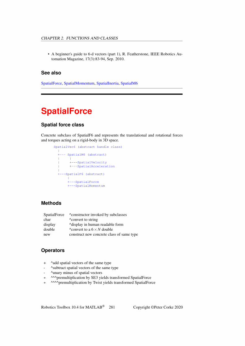
CHAPTER 2. FUNCTIONS AND CLASSES
• A beginner's guide to 6-d vectors (part 1), R. Featherstone, IEEE Robotics Au-tomation Magazine, 17(3):83-94, Sep. 2010.
See also
SpatialForce, SpatialMomentum, SpatialInertia, SpatialM6
SpatialForceSpatial force class
Concrete subclass of SpatialF6 and represents the translational and rotational forcesand torques acting on a rigid-body in 3D space.
SpatialVec6 (abstract handle class)|+--- SpatialM6 (abstract)| || +---SpatialVelocity| +---SpatialAcceleration|+---SpatialF6 (abstract)
|+---SpatialForce+---SpatialMomentum
Methods
SpatialForce ^constructor invoked by subclasseschar ^convert to stringdisplay ^display in human readable formdouble ^convert to a 6×N doublenew construct new concrete class of same type
Operators
+ ^add spatial vectors of the same type- ^subtract spatial vectors of the same type- ^unary minus of spatial vectors* ^^^premultiplication by SE3 yields transformed SpatialForce* ^^^^premultiplication by Twist yields transformed SpatialForce
Robotics Toolbox 10.4 for MATLAB® 281 Copyright ©Peter Corke 2020
CHAPTER 2. FUNCTIONS AND CLASSES
Notes:
• ^is inherited from SpatialVec6.
• ^^is inherited from SpatialM6.
• ^^^are implemented in RTBPose.
• ^^^^are implemented in Twist.
References
• Robot Dynamics Algorithms, R. Featherstone, volume 22, Springer InternationalSeries in Engineering and Computer Science,
• Springer, 1987.
• A beginner's guide to 6-d vectors (part 1), R. Featherstone, IEEE Robotics Au-tomation Magazine, 17(3):83-94, Sep. 2010.
See also
SpatialVec6, SpatialF6, SpatialMomentum
SpatialForce.newConstruct a new object of the same type
A2 = A.new(X) creates a new object of the same type as A, with the value X (6×1).
Notes
• Serves as a dynamic constructor.
• This method is polymorphic across all SpatialVec6 derived classes, and allowseasy creation of a new object of the same class as an existing
• one without needing to explicitly determine its type.
SpatialInertiaSpatial inertia class
Concrete class representing spatial inertia.
Robotics Toolbox 10.4 for MATLAB® 282 Copyright ©Peter Corke 2020
CHAPTER 2. FUNCTIONS AND CLASSES
Methods
SpatialInertia constructorchar convert to stringdisplay display in human readable formdouble convert to a 6×N double
Operators
+ plus: add spatial inertia of connected bodies* mtimes: compute force or momentum
Notes
• Subclass of the MATLAB handle class which means that pass by reference se-mantics apply.
• Spatial inertias can be placed into arrays and indexed.
References
• Robot Dynamics Algorithms, R. Featherstone, volume 22, Springer InternationalSeries in Engineering and Computer Science,
• Springer, 1987.
• A beginner's guide to 6-d vectors (part 1), R. Featherstone, IEEE Robotics Au-tomation Magazine, 17(3):83-94, Sep. 2010.
See also SpatialM6, SpatialF6, SpatialVelocity, SpatialAcceleration, SpatialForce, Spa-tialMomentum.
SpatialInertia.SpatialInertia
Constructor
SI = SpatialInertia(M, C, I) is a spatial inertia object for a rigid-bodywith mass M, centre of mass at C relative to the link frame, and an inertia matrix (3×3)about the centre of mass.
SI = SpatialInertia(I) is a spatial inertia object with a value equal to I (6×6).
Robotics Toolbox 10.4 for MATLAB® 283 Copyright ©Peter Corke 2020
CHAPTER 2. FUNCTIONS AND CLASSES
SpatialInertia.char
Convert to string
s = SI.char() is a string showing spatial inertia parameters in a compact format.If SI is an array of spatial inertia objects return a string with the inertia values in avertical list.
See also
SpatialInertia.display
SpatialInertia.display
Display parameters
SI.display() displays the spatial inertia parameters in compact format. If SI is anarray of spatial inertia objects it displays them in a vertical list.
Notes
• This method is invoked implicitly at the command line when the result of anexpression is a spatial inerita object and the command has
• no trailing semicolon.
See also
SpatialInertia.char
SpatialInertia.double
Convert to matrix
double(V) is a native matrix (6× 6) with the value of the spatial inertia. If V is anarray (1×N) the result is a matrix (6×6×N).
Robotics Toolbox 10.4 for MATLAB® 284 Copyright ©Peter Corke 2020
CHAPTER 2. FUNCTIONS AND CLASSES
SpatialInertia.mtimesMultiplication operator
SI * A is the SpatialForce required for a body with SpatialInertia SI to acceleratewith the SpatialAcceleration A.
SI * V is the SpatialMomemtum of a body with SpatialInertia SI and SpatialVe-locity V.
Notes
• These products must be written in this order, A*SI and V*SI are not defined.
SpatialInertia.plusAddition operator
SI1 + SI2 is the SpatialInertia of a composite body when bodies with SpatialIn-ertia SI1 and SI2 are connected.
SpatialM6Abstract spatial motion class
Abstract superclass that represents spatial motion. This class has two concrete sub-classes:
SpatialVec6 (abstract handle class)|+--- SpatialM6 (abstract)| || +---SpatialVelocity| +---SpatialAcceleration|+---SpatialF6 (abstract)
|+---SpatialForce+---SpatialMomentum
Robotics Toolbox 10.4 for MATLAB® 285 Copyright ©Peter Corke 2020
CHAPTER 2. FUNCTIONS AND CLASSES
Methods
SpatialM6 ^constructor invoked by subclasseschar ^convert to stringcross cross productdisplay ^display in human readable formdouble ^convert to a 6×N double
Operators
+ ^add spatial vectors of the same type- ^subtract spatial vectors of the same type- ^unary minus of spatial vectors
Notes:
• ^is inherited from SpatialVec6.
• Subclass of the MATLAB handle class which means that pass by reference se-mantics apply.
• Spatial vectors can be placed into arrays and indexed.
References
• Robot Dynamics Algorithms, R. Featherstone, volume 22, Springer InternationalSeries in Engineering and Computer Science,
• Springer, 1987.
• A beginner's guide to 6-d vectors (part 1), R. Featherstone, IEEE Robotics Au-tomation Magazine, 17(3):83-94, Sep. 2010.
See also
SpatialForce, SpatialMomentum, SpatialInertia, SpatialM6
SpatialM6.crossSpatial velocity cross product
cross(V1, V2) is a SpatialAcceleration object where V1 and V2 are SpatialM6subclass instances.
cross(V, F) is a SpatialForce object where V1 is a SpatialM6 subclass instancesand F is a SpatialForce subclass instance.
Robotics Toolbox 10.4 for MATLAB® 286 Copyright ©Peter Corke 2020
CHAPTER 2. FUNCTIONS AND CLASSES
Notes
• The first form is Featherstone's “x” operator.
• The second form is Featherstone's “x*” operator.
SpatialMomentumSpatial momentum class
Concrete subclass of SpatialF6 and represents the translational and rotational momen-tum of a rigid-body moving in 3D space.
SpatialVec6 (abstract handle class)|+--- SpatialM6 (abstract)| || +---SpatialVelocity| +---SpatialAcceleration|+---SpatialF6 (abstract)
|+---SpatialForce+---SpatialMomentum
Methods
SpatialMomentum ^constructor invoked by subclassesnew construct new concrete class of same typedouble ^convert to a 6×N doublechar ^convert to stringcross ^^cross productdisplay ^display in human readable form
Operators
+ ^add spatial vectors of the same type- ^subtract spatial vectors of the same type- ^unary minus of spatial vectors
Notes:
• ^is inherited from SpatialVec6.
• ^^is inherited from SpatialM6.
Robotics Toolbox 10.4 for MATLAB® 287 Copyright ©Peter Corke 2020
CHAPTER 2. FUNCTIONS AND CLASSES
References
• Robot Dynamics Algorithms, R. Featherstone, volume 22, Springer InternationalSeries in Engineering and Computer Science,
• Springer, 1987.
• A beginner's guide to 6-d vectors (part 1), R. Featherstone, IEEE Robotics Au-tomation Magazine, 17(3):83-94, Sep. 2010.
See also
SpatialVec6, SpatialF6, SpatialForce
SpatialMomentum.newConstruct a new object of the same type
A2 = A.new(X) creates a new object of the same type as A, with the value X (6×1).
Notes
• Serves as a dynamic constructor.
• This method is polymorphic across all SpatialVec6 derived classes, and allowseasy creation of a new object of the same class as an existing
• one without needing to explicitly determine its type.
SpatialVec6Abstract spatial 6-vector class
Abstract superclass for spatial vector functionality. This class has two abstract sub-classes, which each have concrete subclasses:
SpatialVec6 (abstract handle class)
|+--- SpatialM6 (abstract)| || +---SpatialVelocity| +---SpatialAcceleration|+---SpatialF6 (abstract)
Robotics Toolbox 10.4 for MATLAB® 288 Copyright ©Peter Corke 2020
CHAPTER 2. FUNCTIONS AND CLASSES
|+---SpatialForce+---SpatialMomentum
Methods
SpatialV6 constructor invoked by subclassesdouble convert to a 6×N doublechar convert to stringdisplay display in human readable form
Operators
+ add spatial vectors of the same type- subtract spatial vectors of the same type- unary minus of spatial vectors
Notes
• Subclass of the MATLAB handle class which means that pass by reference se-mantics apply.
• Spatial vectors can be placed into arrays and indexed.
References
• Robot Dynamics Algorithms, R. Featherstone, volume 22, Springer InternationalSeries in Engineering and Computer Science,
• Springer, 1987.
• A beginner's guide to 6-d vectors (part 1), R. Featherstone, IEEE Robotics Au-tomation Magazine, 17(3):83-94, Sep. 2010.
See also SpatialM6, SpatialF6, SpatialVelocity, SpatialAcceleration, SpatialForce, Spa-tialMomentum, SpatialInertia.
SpatialVec6.SpatialVec6Constructor
SpatiaVecXXX(V) is a spatial vector of type SpatiaVecXXX with a value from V(6×1). If V (6×N) then an (N ×1) array of spatial vectors is returned.
This constructor is inherited by all the concrete subclasses.
Robotics Toolbox 10.4 for MATLAB® 289 Copyright ©Peter Corke 2020
CHAPTER 2. FUNCTIONS AND CLASSES
See also
SpatialVelocity, SpatialAcceleration, SpatialForce, SpatialMomentum
SpatialVec6.charConvert to string
s = V.char() is a string showing spatial vector parameters in a compact singleline format. If V is an array of spatial vector objects return a string with one line perelement.
See also
SpatialVec6.display
SpatialVec6.displayDisplay parameters
V.display() displays the spatial vector parameters in compact single line format.If V is an array of spatial vector objects it displays one per line.
Notes
• This method is invoked implicitly at the command line when the result of anexpression is a serial vector subclass object and the command has
• no trailing semicolon.
See also
SpatialVec6.char
SpatialVec6.doubleConvert to matrix
double(V) is a native matrix (6× 1) with the value of the spatial vector. If V is anarray (1×N) the result is a matrix (6×N).
Robotics Toolbox 10.4 for MATLAB® 290 Copyright ©Peter Corke 2020
CHAPTER 2. FUNCTIONS AND CLASSES
SpatialVec6.minusSubtraction operator
V1 - V2 is a spatial vector of the same type as V1 and V2 whose value is the differ-ence of V1 and V2. If both are arrays of spatial vectors V1 (1×N) and V2 (1×N) theresult is an array (1×N).
See also
SpatialVec6.uminus, SpatialVec6.plus
SpatialVec6.plusAddition operator
V1 + V2 is a spatial vector of the same type as V1 and V2 whose value is the sum ofV1 and V2. If both are arrays of spatial vectors V1 (1×N) and V2 (1×N) the result isan array (1×N).
See also
SpatialVec6.minus
SpatialVec6.uminusUnary minus operator
• V is a spatial vector of the same type as V whose value is
the negative of V. If V is an array V (1×N) then the result is an array (1×N).
See also
SpatialVec6.minus, SpatialVec6.plus
Robotics Toolbox 10.4 for MATLAB® 291 Copyright ©Peter Corke 2020
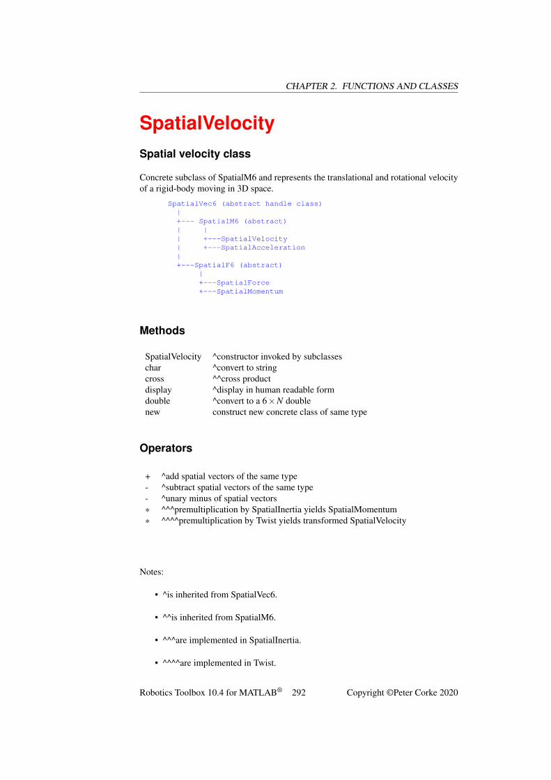
CHAPTER 2. FUNCTIONS AND CLASSES
SpatialVelocitySpatial velocity class
Concrete subclass of SpatialM6 and represents the translational and rotational velocityof a rigid-body moving in 3D space.
SpatialVec6 (abstract handle class)|+--- SpatialM6 (abstract)| || +---SpatialVelocity| +---SpatialAcceleration|+---SpatialF6 (abstract)
|+---SpatialForce+---SpatialMomentum
Methods
SpatialVelocity ^constructor invoked by subclasseschar ^convert to stringcross ^^cross productdisplay ^display in human readable formdouble ^convert to a 6×N doublenew construct new concrete class of same type
Operators
+ ^add spatial vectors of the same type- ^subtract spatial vectors of the same type- ^unary minus of spatial vectors* ^^^premultiplication by SpatialInertia yields SpatialMomentum* ^^^^premultiplication by Twist yields transformed SpatialVelocity
Notes:
• ^is inherited from SpatialVec6.
• ^^is inherited from SpatialM6.
• ^^^are implemented in SpatialInertia.
• ^^^^are implemented in Twist.
Robotics Toolbox 10.4 for MATLAB® 292 Copyright ©Peter Corke 2020
CHAPTER 2. FUNCTIONS AND CLASSES
References
• Robot Dynamics Algorithms, R. Featherstone, volume 22, Springer InternationalSeries in Engineering and Computer Science,
• Springer, 1987.
• A beginner's guide to 6-d vectors (part 1), R. Featherstone, IEEE Robotics Au-tomation Magazine, 17(3):83-94, Sep. 2010.
See also
SpatialVec6, SpatialM6, SpatialAcceleration, SpatialInertia, SpatialMomentum
SpatialVelocity.newConstruct a new object of the same type
A2 = A.new(X) creates a new object of the same type as A, with the value X (6×1).
Notes
• Serves as a dynamic constructor.
• This method is polymorphic across all SpatialVec6 derived classes, and allowseasy creation of a new object of the same class as an existing
• one without needing to explicitly determine its type.
stlReadReads STL file
[v, f, n, objname] = stlRead(fileName) reads the STL format file (ASCIIor binary) and returns:
V (Mx3) each row is the 3D coordinate of a vertexF (Nx3) each row is a list of vertex indices that defines a triangular faceN (Nx3) each row is a unit-vector defining the face normalOBJNAME is the name of the STL object (NOT the name of the STL file).
Robotics Toolbox 10.4 for MATLAB® 293 Copyright ©Peter Corke 2020
CHAPTER 2. FUNCTIONS AND CLASSES
Authors
• From MATLAB File Exchange by Pau Mico, https://au.mathworks.com/matlabcentral/fileexchange/51200-stltools
• Copyright (c) 2015, Pau Mico
• Copyright (c) 2013, Adam H. Aitkenhead
• Copyright (c) 2011, Francis Esmonde-White
t2rRotational submatrix
R = T2R(T) is the orthonormal rotation matrix component of homogeneous trans-formation matrix T. Works for T in SE(2) or SE(3)
• If T is 4×4, then R is 3×3.
• If T is 3×3, then R is 2×2.
Notes
• For a homogeneous transform sequence (K ×K ×N) returns a rotation matrixsequence (K −1×K-1×N).
• The validity of rotational part is not checked
See also
r2t, tr2rt, rt2tr
tb_optparseStandard option parser for Toolbox functions
OPTOUT = TB_OPTPARSE(OPT, ARGLIST) is a generalized option parser forToolbox functions. OPT is a structure that contains the names and default values forthe options, and ARGLIST is a cell array containing option parameters, typically itcomes from VARARGIN. It supports options that have an assigned value, boolean orenumeration types (string or int).
Robotics Toolbox 10.4 for MATLAB® 294 Copyright ©Peter Corke 2020
CHAPTER 2. FUNCTIONS AND CLASSES
[OPTOUT,ARGS] = TB_OPTPARSE(OPT, ARGLIST) as above but returns allthe unassigned options, those that don't match anything in OPT, as a cell array of allunassigned arguments in the order given in ARGLIST.
[OPTOUT,ARGS,LS] = TB_OPTPARSE(OPT, ARGLIST) as above but if anyunmatched option looks like a MATLAB LineSpec (eg. 'r:') it is placed in LS ratherthan in ARGS.
[OBJOUT,ARGS,LS] = TB_OPTPARSE(OPT, ARGLIST, OBJ) as above butproperties of OBJ with matching names in OPT are set.
The software pattern is:
function myFunction(a, b, c, varargin)opt.foo = false;opt.bar = true;opt.blah = [];opt.stuff = {};opt.choose = {’this’, ’that’, ’other’};opt.select = {’#no’, ’#yes’};opt.old = ’@foo’;opt = tb_optparse(opt, varargin);
Optional arguments to the function behave as follows:
'foo' sets opt.foo := true'nobar' sets opt.foo := false'blah', 3 sets opt.blah := 3'blah',x,y sets opt.blah := {x,y}'that' sets opt.choose := 'that''yes' sets opt.select := 2 (the second element)'stuff', 5 sets opt.stuff to {5}'stuff', 'k',3 sets opt.stuff to {'k',3}'old' synonym, is the same as the option foo
and can be given in any combination.
If neither of 'this', 'that'or 'other'are specified then opt.choose := 'this'. Alternatively if:
opt.choose = {[], ’this’, ’that’, ’other’};
then if neither of 'this', 'that'or 'other'are specified then opt.choose := [].
If neither of 'no'or 'yes'are specified then opt.select := 1.
The return structure is automatically populated with fields: verbose and debug. Thefollowing options are automatically parsed:
'verbose' sets opt.verbose := true'verbose=2' sets opt.verbose := 2 (very verbose)'verbose=3' sets opt.verbose := 3 (extremeley verbose)'verbose=4' sets opt.verbose := 4 (ridiculously verbose)'debug', N sets opt.debug := N'showopt' displays opt and arglist'setopt',S opt.foo is set to 4. sets opt := S, if S.foo=4, and opt.foo is present, then
Robotics Toolbox 10.4 for MATLAB® 295 Copyright ©Peter Corke 2020
CHAPTER 2. FUNCTIONS AND CLASSES
The allowable options are specified by the names of the fields in the structure OPT. Bydefault if an option is given that is not a field of OPT an error is declared.
Notes
• That the enumerator names must be distinct from the field names.
• That only one value can be assigned to a field, if multiple values are requiredthey must placed in a cell array.
• If the option is seen multiple times the last (rightmost) instance applies.
• To match an option that starts with a digit, prefix it with 'd_', so the field 'd_3d'matchesthe option '3d'.
• Any input argument or element of the opt struct can be a string instead of a chararray.
tr2angvecConvert rotation matrix to angle-vector form
[THETA,V] = TR2ANGVEC(R, OPTIONS) is rotation expressed in terms of anangle THETA (1× 1) about the axis V (1× 3) equivalent to the orthonormal rotationmatrix R (3×3).
[THETA,V] = TR2ANGVEC(T, OPTIONS) as above but uses the rotational partof the homogeneous transform T (4×4).
If R (3×3×K) or T (4×4×K) represent a sequence then THETA (K×1)is a vector ofangles for corresponding elements of the sequence and V (K×3) are the correspondingaxes, one per row.
Options
'deg' Return angle in degrees (default radians)
Notes
• For an identity rotation matrix both THETA and V are set to zero.
• The rotation angle is always in the interval [0 π], negative rotation is handled byinverting the direction of the rotation axis.
• If no output arguments are specified the result is displayed.
Robotics Toolbox 10.4 for MATLAB® 296 Copyright ©Peter Corke 2020
CHAPTER 2. FUNCTIONS AND CLASSES
See also
angvec2r, angvec2tr, trlog
tr2delta
Convert SE(3) homogeneous transform to differential motion
D = TR2DELTA(T0, T1) is the differential motion (6× 1) corresponding to in-finitessimal motion (in the T0 frame) from pose T0 to T1 which are homogeneoustransformations (4×4) or SE3 objects.
The vector D=(dx, dy, dz, dRx, dRy, dRz) represents infinitessimal translation androtation, and is an approximation to the instantaneous spatial velocity multiplied bytime step.
D = TR2DELTA(T) as above but the motion is from the world frame to the SE3 poseT.
Notes
• D is only an approximation to the motion T, and assumes that T0≈T1 or T≈eye(4,4).
• Can be considered as an approximation to the effect of spatial velocity over a atime interval, average spatial velocity multiplied by time.
Reference
• Robotics, Vision & Control: Second Edition, P. Corke, Springer 2016; p67.
See also
delta2tr, skew, SE3.todelta
Robotics Toolbox 10.4 for MATLAB® 297 Copyright ©Peter Corke 2020
CHAPTER 2. FUNCTIONS AND CLASSES
tr2eulConvert SO(3) or SE(3) matrix to Euler angles
EUL = TR2EUL(T, OPTIONS) are the ZYZ Euler angles (1×3) corresponding tothe rotational part of a homogeneous transform T (4×4). The 3 angles EUL=[PHI,THETA,PSI]correspond to sequential rotations about the Z, Y and Z axes respectively.
EUL = TR2EUL(R, OPTIONS) as above but the input is an orthonormal rotationmatrix R (3×3).
If R (3×3×K) or T (4×4×K) represent a sequence then each row of EUL correspondsto a step of the sequence.
Options
'deg' Compute angles in degrees (radians default)'flip' Choose first Euler angle to be in quadrant 2 or 3.
Notes
• There is a singularity for the case where THETA=0 in which case PHI is arbi-trarily set to zero and PSI is the sum (PHI+PSI).
• Translation component is ignored.
See also
eul2tr, tr2rpy
tr2jacJacobian for differential motion
J = TR2JAC(TAB) is a Jacobian matrix (6×6) that maps spatial velocity or differ-ential motion from frame {A} to frame {B} where the pose of {B} relative to {A} isrepresented by the homogeneous transform TAB (4×4).
J = TR2JAC(TAB, ’samebody’) is a Jacobian matrix (6×6) that maps spatialvelocity or differential motion from frame {A} to frame {B} where both are attachedto the same moving body. The pose of {B} relative to {A} is represented by the homo-geneous transform TAB (4×4).
Robotics Toolbox 10.4 for MATLAB® 298 Copyright ©Peter Corke 2020
CHAPTER 2. FUNCTIONS AND CLASSES
See also
wtrans, tr2delta, delta2tr, SE3.velxform
tr2rpyConvert SO(3) or SE(3) matrix to roll-pitch-yaw angles
RPY = TR2RPY(T, options) are the roll-pitch-yaw angles (1× 3) correspond-ing to the rotation part of a homogeneous transform T. The 3 angles RPY=[ROLL,PITCH,YAW]correspond to sequential rotations about the Z, Y and X axes respectively. Roll and yawangles are in [−π,π) while pitch angle is in [-π/2,π/2).
RPY = TR2RPY(R, options) as above but the input is an orthonormal rotationmatrix R (3×3).
If R (3×3×K) or T (4×4×K) represent a sequence then each row of RPY correspondsto a step of the sequence.
Options
'deg' Compute angles in degrees (radians default)
'xyz' Return solution for sequential rotations about X, Y, Z axes'zyx' Return solution for sequential rotations about Z, Y, X axes (default)'yxz' Return solution for sequential rotations about Y, X, Z axes'arm' Return solution for sequential rotations about X, Y, Z axes'vehicle' Return solution for sequential rotations about Z, Y, X axes'camera' Return solution for sequential rotations about Y, X, Z axes
Notes
• There is a singularity for the case where PITCH=π/2 in which case ROLL isarbitrarily set to zero and YAW is the sum (ROLL+YAW).
• Translation component is ignored.
• Toolbox rel 8-9 has XYZ angle sequence as default.
• 'arm', 'vehicle', 'camera'are synonyms for 'xyz', 'zyx'and 'yxz'respectively.
• these solutions are generated by symbolic/rpygen.mlx
Robotics Toolbox 10.4 for MATLAB® 299 Copyright ©Peter Corke 2020
CHAPTER 2. FUNCTIONS AND CLASSES
See also
rpy2tr, tr2eul
tr2rtConvert homogeneous transform to rotation and translation
[R,t] = TR2RT(TR) splits a homogeneous transformation matrix (N × N) intoan orthonormal rotation matrix R (M ×M) and a translation vector t (M × 1), whereN=M+1.
Works for TR in SE(2) or SE(3)
• If TR is 4×4, then R is 3×3 and T is 3×1.
• If TR is 3×3, then R is 2×2 and T is 2×1.
A homogeneous transform sequence TR (N ×N ×K) is split into rotation matrix se-quence R (M×M×K) and a translation sequence t (K ×M).
Notes
• The validity of R is not checked.
See also
rt2tr, r2t, t2r
tranimateAnimate a 3D coordinate frame
TRANIMATE(P1, P2, OPTIONS) animates a 3D coordinate frame moving frompose X1 to pose X2. Poses X1 and X2 can be represented by:
• SE(3) homogeneous transformation matrices (4×4)
• SO(3) orthonormal rotation matrices (3×3)
Robotics Toolbox 10.4 for MATLAB® 300 Copyright ©Peter Corke 2020
CHAPTER 2. FUNCTIONS AND CLASSES
TRANIMATE(X, OPTIONS) animates a coordinate frame moving from the identitypose to the pose X represented by any of the types listed above.
TRANIMATE(XSEQ, OPTIONS) animates a trajectory, where XSEQ is any of
• SE(3) homogeneous transformation matrix sequence (4×4×N)
• SO(3) orthonormal rotation matrix sequence (3×3×N)
Options
'fps', fps Number of frames per second to display (default 10)'nsteps', n The number of steps along the path (default 50)'axis',A Axis bounds [xmin, xmax, ymin, ymax, zmin, zmax]'movie',M Save frames as a movie or sequence of frames'cleanup' Remove the frame at end of animation'noxyz' Don't label the axes'rgb' Color the axes in the order x=red, y=green, z=blue'retain' Retain frames, don't animate
Additional options are passed through to TRPLOT.
Notes
• Uses the Animate helper class to record the frames.
See also
trplot, Animate, SE3.animate
tranimate2Animate a 2D coordinate frame
TRANIMATE2(P1, P2, OPTIONS) animates a 3D coordinate frame moving frompose X1 to pose X2. Poses X1 and X2 can be represented by:
• SE(2) homogeneous transformation matrices (3×3)
• SO(2) orthonormal rotation matrices (2×2)
TRANIMATE2(X, OPTIONS) animates a coordinate frame moving from the iden-tity pose to the pose X represented by any of the types listed above.
TRANIMATE2(XSEQ, OPTIONS) animates a trajectory, where XSEQ is any of
Robotics Toolbox 10.4 for MATLAB® 301 Copyright ©Peter Corke 2020
CHAPTER 2. FUNCTIONS AND CLASSES
• SE(2) homogeneous transformation matrix sequence (3×3×N)
• SO(2) orthonormal rotation matrix sequence (2×2×N)
Options
'fps', fps Number of frames per second to display (default 10)'nsteps', n The number of steps along the path (default 50)'axis',A Axis bounds [xmin, xmax, ymin, ymax, zmin, zmax]'movie',M Save frames as a movie or sequence of frames'cleanup' Remove the frame at end of animation'noxyz' Don't label the axes'rgb' Color the axes in the order x=red, y=green, z=blue'retain' Retain frames, don't animate
Additional options are passed through to TRPLOT2.
Notes
• Uses the Animate helper class to record the frames.
See also
trplot, Animate, SE3.animate
transl
SE(3) translational homogeneous transform
Create a translational SE(3) matrix
T = TRANSL(X, Y, Z) is an SE(3) homogeneous transform (4×4) representinga pure translation of X, Y and Z.
T = TRANSL(P) is an SE(3) homogeneous transform (4×4) representing a transla-tion of P=[X,Y,Z]. P (M×3) represents a sequence and T (4×4×M) is a sequence ofhomogeneous transforms such that T(:,:,i) corresponds to the i'th row of P.
Robotics Toolbox 10.4 for MATLAB® 302 Copyright ©Peter Corke 2020
CHAPTER 2. FUNCTIONS AND CLASSES
Extract the translational part of an SE(3) matrix
P = TRANSL(T) is the translational part of a homogeneous transform T as a 3-element column vector. T (4× 4×M) is a homogeneous transform sequence and therows of P (M × 3) are the translational component of the corresponding transform inthe sequence.
[X,Y,Z] = TRANSL(T) is the translational part of a homogeneous transform Tas three components. If T (4 × 4 ×M) is a homogeneous transform sequence thenX,Y,Z (1×M) are the translational components of the corresponding transform in thesequence.
Notes
• Somewhat unusually, this function performs a function and its inverse. An his-torical anomaly.
See also
SE3.t, SE3.transl
transl2SE(2) translational homogeneous transform
Create a translational SE(2) matrix
T = TRANSL2(X, Y) is an SE(2) homogeneous transform (3× 3) representing apure translation.
T = TRANSL2(P) is a homogeneous transform representing a translation or pointP=[X,Y]. P (M×2) represents a sequence and T (3×3×M) is a sequence of homoge-nous transforms such that T(:,:,i) corresponds to the i'th row of P.
Extract the translational part of an SE(2) matrix
P = TRANSL2(T) is the translational part of a homogeneous transform as a 2-elementcolumn vector. T (3× 3×M) is a homogeneous transform sequence and the rows ofP (M × 2) are the translational component of the corresponding transform in the se-quence.
Robotics Toolbox 10.4 for MATLAB® 303 Copyright ©Peter Corke 2020
CHAPTER 2. FUNCTIONS AND CLASSES
Notes
• Somewhat unusually, this function performs a function and its inverse. An his-torical anomaly.
See also
SE2.t, rot2, ishomog2, trplot2, transl
trchainCompound SE(3) transforms from string
T = TRCHAIN(S) is a homogeneous transform (4×4) that results from compound-ing a number of elementary transformations defined by the string S. The string S com-prises a number of tokens of the form X(ARG) where X is one of Tx, Ty, Tz, Rx, Ry, orRz. ARG is an arbitrary MATLAB expression that can include constants or workspacevariables. For example:
trchain(’Tx(1) Rx(90) Ry(45) Tz(2)’)
is equivalent to computing
transl(1,0,0) * trotx(90, ’deg’) * troty(45, ’deg’) * transl(0,0,2)
T = TRCHAIN(S, Q) as above but the expression for ARG can also contain a vari-able 'qJ'which selects the Jth value from the passed vector Q (1×N). For example:
trchain(’Rx(q1)Tx(a1)Ry(q2)Ty(a3)Rz(q3)’, [1 2 3])
[T,TOK] = TRCHAIN(S ...) as above but return an array of tokens which can be passedin, instead of the string.
T = TRCHAIN(TOK ...) as above but chain is defined by array of tokens instead of astring.
Options
- 'deg' all angular variables are in degrees (default radians)- 'qvar',V treat the string V as the joint variable name rather than 'q'
Robotics Toolbox 10.4 for MATLAB® 304 Copyright ©Peter Corke 2020
CHAPTER 2. FUNCTIONS AND CLASSES
Notes
• Variables used in the string must exist in the caller workspace.
• The string can contain arbitrary characters between the elements, for examplespace, +, *, . or even |.
• Works for symbolic variables in the workspace and/or passed in via the vector Q.
• For symbolic operations that involve use of the value π , make sure you define itfirst in the workspace: π = sym('π ');
• The tokens are simply a parsed version of the input string and provide someefficiency for repeated calls on the same chain.
See also
trchain2, trotx, troty, trotz, transl, SerialLink.trchain, ETS
trchain2
Compound SE(2) transforms from string
T = TRCHAIN(S) is a homogeneous transform (3×3) that results from compound-ing a number of elementary transformations defined by the string S. The string S com-prises a number of tokens of the form X(ARG) where X is one of Tx, Ty, or R. ARGis an arbitrary MATLAB expression that can include constants or workspace variables.For example:
trchain(’Tx(1) R(90) Ty(2)’)
is equivalent to computing
transl2(1,0) * trot2(90, ’deg’) * transl2(0,2)
T = TRCHAIN(S, Q) as above but the expression for ARG can also contain a vari-able 'qJ'which selects the Jth value from the passed vector Q (1×N). For example:
trchain(’Tx(1) R(q1-90) Ty(2) R(q2)’, [1 2])
[T,TOK] = TRCHAIN(S ...) as above but return an array of tokens which can be passedin, instead of the string.
T = TRCHAIN(TOK ...) as above but chain is defined by array of tokens instead of astring.
Robotics Toolbox 10.4 for MATLAB® 305 Copyright ©Peter Corke 2020
CHAPTER 2. FUNCTIONS AND CLASSES
Options
- 'deg' all angular variables are in degrees (default radians)- 'qvar',V treat the string V as the joint variable name rather than 'q'
Notes
• Variables used in the string must exist in the caller workspace.
• The string can contain arbitrary characters between the elements, for examplespace, +, *, . or even |.
• Works for symbolic variables in the workspace and/or passed in via the vector Q.
• For symbolic operations that involve use of the value π , make sure you define itfirst in the workspace: π = sym('π ');
• The tokens are simply a parsed version of the input string and provide someefficiency for repeated calls on the same chain.
See also
trchain2, trotx, troty, trotz, transl, SerialLink.trchain, ETS
trexpMatrix exponential for so(3) and se(3)
For so(3)
R = TREXP(OMEGA) is the matrix exponential (3×3) of the so(3) element OMEGAthat yields a rotation matrix (3×3).
R = TREXP(OMEGA, THETA) as above, but so(3) motion of THETA*OMEGA.
R = TREXP(S, THETA) as above, but rotation of THETA about the unit vector S.
R = TREXP(W) as above, but the so(3) value is expressed as a vector W (1×3) whereW = S * THETA. Rotation by ||W|| about the vector W.
For se(3)
T = TREXP(SIGMA) is the matrix exponential (4×4) of the se(3) element SIGMAthat yields a homogeneous transformation matrix (4×4).
Robotics Toolbox 10.4 for MATLAB® 306 Copyright ©Peter Corke 2020
CHAPTER 2. FUNCTIONS AND CLASSES
T = TREXP(SIGMA, THETA) as above, but se(3) motion of SIGMA*THETA, therotation part of SIGMA (4×4) must be unit norm.
T = TREXP(TW) as above, but the se(3) value is expressed as a twist vector TW(1×6).
T = TREXP(TW, THETA) as above, but se(3) motion of TW*THETA, the rotationpart of TW (1×6) must be unit norm.
Notes
• Efficient closed-form solution of the matrix exponential for arguments that areso(3) or se(3).
• If THETA is given then the first argument must be a unit vector or a skew-symmetric matrix from a unit vector.
• Angle vector argument order is different to ANGVEC2R.
References
• Robotics, Vision & Control: Second Edition, P. Corke, Springer 2016; p42-43.
• Mechanics, planning and control, Park & Lynch, Cambridge, 2017.
See also
angvec2r, trlog, trexp2, skew, skewa, Twist
trexp2
Matrix exponential for so(2) and se(2)
SO(2)
R = TREXP2(OMEGA) is the matrix exponential (2×2) of the so(2) element OMEGAthat yields a rotation matrix (2×2).
R = TREXP2(THETA) as above, but rotation by THETA (1×1).
Robotics Toolbox 10.4 for MATLAB® 307 Copyright ©Peter Corke 2020
CHAPTER 2. FUNCTIONS AND CLASSES
SE(2)
T = TREXP2(SIGMA) is the matrix exponential (3×3) of the se(2) element SIGMAthat yields a homogeneous transformation matrix (3×3).
T = TREXP2(SIGMA, THETA) as above, but se(2) rotation of SIGMA*THETA,the rotation part of SIGMA (3×3) must be unit norm.
T = TREXP2(TW) as above, but the se(2) value is expressed as a vector TW (1×3).
T = TREXP(TW, THETA) as above, but se(2) rotation of TW*THETA, the rotationpart of TW must be unit norm.
Notes
• Efficient closed-form solution of the matrix exponential for arguments that areso(2) or se(2).
• If THETA is given then the first argument must be a unit vector or a skew-symmetric matrix from a unit vector.
References
• Robotics, Vision & Control: Second Edition, P. Corke, Springer 2016; p25-26.
• Mechanics, planning and control, Park & Lynch, Cambridge, 2017.
See also
trexp, skew, skewa, Twist
trinterpInterpolate SE(3) homogeneous transformations
TRINTERP(T0, T1, S) is a homogeneous transform (4×4) interpolated betweenT0 when S=0 and T1 when S=1. T0 and T1 are both homogeneous transforms (4×4).If S (N×1) then T (4×4×N) is a sequence of homogeneous transforms correspondingto the interpolation values in S.
TRINTERP(T1, S) as above but interpolated between the identity matrix when S=0to T1 when S=1.
TRINTERP(T0, T1, M) as above but M is a positive integer and return a sequence(4×4×M) of homogeneous transforms linearly interpolating between T0 and T1 in Msteps.
Robotics Toolbox 10.4 for MATLAB® 308 Copyright ©Peter Corke 2020
CHAPTER 2. FUNCTIONS AND CLASSES
TRINTERP(T1, M) as above but return a sequence (4 × 4 × M) of homogeneousinterpolating between identity matrix and T1 in M steps.
Notes
• T0 or T1 can also be an SO(3) rotation matrix (3×3) in which case the result is(3×3×N).
• Rotation is interpolated using quaternion spherical linear interpolation (slerp).
• To obtain smooth continuous motion S should also be smooth and continuous,such as computed by tpoly or lspb.
See also
trinterp2, ctraj, SE3.interp, UnitQuaternion, tpoly, lspb
trinterp2Interpolate SE(2) homogeneous transformations
TRINTERP2(T0, T1, S) is a homogeneous transform (3 × 3) interpolated be-tween T0 when S=0 and T1 when S=1. T0 and T1 are both homogeneous transforms(4× 4). If S (N × 1) then T (3× 3×N) is a sequence of homogeneous transformscorresponding to the interpolation values in S.
TRINTERP2(T1, S) as above but interpolated between the identity matrix whenS=0 to T1 when S=1.
TRINTERP2(T0, T1, M) as above but M is a positive integer and return a sequence(4×4×M) of homogeneous transforms linearly interpolating between T0 and T1 in Msteps.
TRINTERP2(T1, M) as above but return a sequence (4× 4×M) of homogeneousinterpolating between identity matrix and T1 in M steps.
Notes
• T0 or T1 can also be an SO(2) rotation matrix (2×2).
• Rotation angle is linearly interpolated.
• To obtain smooth continuous motion S should also be smooth and continuous,such as computed by tpoly or lspb.
Robotics Toolbox 10.4 for MATLAB® 309 Copyright ©Peter Corke 2020
CHAPTER 2. FUNCTIONS AND CLASSES
See also
trinterp, SE3.interp, UnitQuaternion, tpoly, lspb
trlogLogarithm of SO(3) or SE(3) matrix
S = trlog(R) is the matrix logarithm (3×3) of R (3×3) which is a skew symmet-ric matrix corresponding to the vector theta*w where theta is the rotation angle and w(3×1) is a unit-vector indicating the rotation axis.
[theta,w] = trlog(R) as above but returns directly theta the rotation angleand w (3×1) the unit-vector indicating the rotation axis.
S = trlog(T) is the matrix logarithm (4 × 4) of T (4 × 4) which has a skew-symmetric upper-left 3 × 3 submatrix corresponding to the vector theta*w wheretheta is the rotation angle and w (3×1) is a unit-vector indicating the rotation axis,and a translation component.
[theta,twist] = trlog(T) as above but returns directly theta the rotationangle and a twist vector (6×1) comprising [v w].
Notes
• Efficient closed-form solution of the matrix logarithm for arguments that areSO(3) or SE(3).
• Special cases of rotation by odd multiples of π are handled.
• Angle is always in the interval [0,π].
• There is no Toolbox function for SO(2) or SE(2), use LOGM instead.
References
• Robotics, Vision & Control: Second Edition, P. Corke, Springer 2016; p43.
• Mechanics, planning and control, Park & Lynch, Cambridge, 2016.
See also
trexp, trexp2, Twist, logm
Robotics Toolbox 10.4 for MATLAB® 310 Copyright ©Peter Corke 2020
CHAPTER 2. FUNCTIONS AND CLASSES
trnorm
Normalize an SO(3) or SE(3) matrix
TRNORM(R) is guaranteed to be a proper orthogonal matrix rotation matrix (3× 3)which is “close” to the input matrix R (3×3). If R = [N,O,A] the O and A vectors aremade unit length and the normal vector is formed from N = O x A, and then we ensurethat O and A are orthogonal by O = A x N.
TRNORM(T) as above but the rotational submatrix of the homogeneous transformationT (4×4) is normalised while the translational part is unchanged.
If R (3× 3×K) or T (4× 4×K) representing a sequence then the normalisation isperformed on each of the K planes.
Notes
• Only the direction of A (the z-axis) is unchanged.
• Used to prevent finite word length arithmetic causing transforms to become ‘un-normalized'.
• There is no Toolbox function for SO(2) or SE(2).
See also
oa2tr, SO3.trnorm, SE3.trnorm
trot2
SE(2) rotation matrix
T = TROT2(THETA) is a homogeneous transformation (3× 3) representing a rota-tion of THETA radians.
T = TROT2(THETA, ’deg’) as above but THETA is in degrees.
Notes
• Translational component is zero.
Robotics Toolbox 10.4 for MATLAB® 311 Copyright ©Peter Corke 2020
CHAPTER 2. FUNCTIONS AND CLASSES
See also
rot2, transl2, ishomog2, trplot2, trotx, troty, trotz, SE2
trotx
SE(3) rotation about X axis
T = TROTX(THETA) is a homogeneous transformation (4× 4) representing a rota-tion of THETA radians about the x-axis.
T = TROTX(THETA, ’deg’) as above but THETA is in degrees.
Notes
• Translational component is zero.
See also
rotx, troty, trotz, trot2, SE3.Rx
troty
SE(3) rotation about Y axis
T = troty(THETA) is a homogeneous transformation (4× 4) representing a rota-tion of THETA radians about the y-axis.
T = troty(THETA, ’deg’) as above but THETA is in degrees.
Notes
• Translational component is zero.
Robotics Toolbox 10.4 for MATLAB® 312 Copyright ©Peter Corke 2020
CHAPTER 2. FUNCTIONS AND CLASSES
See also
roty, trotx, trotz, trot2, SE3.Ry
trotz
SE(3) rotation about Z axis
T = trotz(THETA) is a homogeneous transformation (4× 4) representing a rota-tion of THETA radians about the z-axis.
T = trotz(THETA, ’deg’) as above but THETA is in degrees.
Notes
• Translational component is zero.
See also
rotz, trotx, troty, trot2, SE3.Rz
trplot
Plot a 3D coordinate frame
TRPLOT(T, OPTIONS) draws a 3D coordinate frame represented by the SE(3) ho-mogeneous transform T (4×4).
H = TRPLOT(T, OPTIONS) as above but returns a handle.
TRPLOT(R, OPTIONS) as above but the coordinate frame is rotated about the originaccording to the orthonormal rotation matrix R (3×3).
H = TRPLOT(R, OPTIONS) as above but returns a handle.
H = TRPLOT() creates a default frame EYE(3,3) at the origin and returns a handle.
Robotics Toolbox 10.4 for MATLAB® 313 Copyright ©Peter Corke 2020
CHAPTER 2. FUNCTIONS AND CLASSES
Animation
Firstly, create a plot and keep the the handle as per above.
TRPLOT(H, T) moves the coordinate frame described by the handle H to the pose T(4×4).
Options
'handle',h Update the specified handle'axhandle',A Draw in the MATLAB axes specified by the axis handle A
'color',C The color to draw the axes, MATLAB ColorSpec'axes' Show the MATLAB axes, box and ticks (default true)'axis',A Set dimensions of the MATLAB axes to A=[xmin xmax ymin ymax zmin zmax]'frame',F The coordinate frame is named {F} and the subscript on the axis labels is F.'framelabel',F The coordinate frame is named {F}, axes have no subscripts.'framelabeloffset',O Offset O=[DX DY] frame labels in units of text box height'text_opts', opt A cell array of MATLAB text properties'length',s Length of the coordinate frame arms (default 1)'thick',t Thickness of lines (default 0.5)'text' Enable display of X,Y,Z labels on the frame (default true)'labels',L Label the X,Y,Z axes with the 1st, 2nd, 3rd character of the string L'rgb' Display X,Y,Z axes in colors red, green, blue respectively'rviz' Display chunky rviz style axes%'arrow' Use arrows rather than line segments for the axes'width', w Width of arrow tips (default 1)
'perspective' Display the axes with perspective projection (default off)'3d' Plot in 3D using anaglyph graphics'anaglyph',A left and right (default colors 'rc'): chosen from Specify anaglyph colors for '3d'as 2 characters for
r)ed, g)reen, b)lue, c)yan, m)agenta.'dispar',D Disparity for 3d display (default 0.1)'view',V for view toward origin of coordinate frame Set plot view parameters V=[az el] angles, or 'auto''lefty' Draw left-handed frame (dangerous)
Examples
trplot(T, ’frame’, ’A’) trplot(T, 'frame', 'A', 'color', 'b') trplot(T1, 'frame','A', 'text_opts', {'FontSize', 10, 'FontWeight', 'bold'}) trplot(T1, 'labels', 'NOA');
h = trplot(T, ’frame’, ’A’, ’color’, ’b’); trplot(h, T2);
3D anaglyph plot
trplot(T, ’3d’);
Robotics Toolbox 10.4 for MATLAB® 314 Copyright ©Peter Corke 2020
CHAPTER 2. FUNCTIONS AND CLASSES
Notes
• Multiple frames can be added using the HOLD command
• When animating a coordinate frame it is best to set the axis bounds initially.
• The 'rviz'option is equivalent to 'rgb', 'notext', 'noarrow', 'thick', 5.
• The 'arrow'option requires https://www.mathworks.com/matlabcentral/fileexchange/14056-arrow3
trplot2Plot a 2D coordinate frame
TRPLOT2(T, OPTIONS) draws a 2D coordinate frame represented by the SE(2)homogeneous transform T (3×3).
H = TRPLOT2(T, OPTIONS) as above but returns a handle.
TRPLOT(R, OPTIONS) as above but the coordinate frame is rotated about the originaccording to the orthonormal rotation matrix R (2×2).
H = TRPLOT(R, OPTIONS) as above but returns a handle.
H = TRPLOT2() creates a default frame EYE(2,2) at the origin and returns a handle.
Animation
Firstly, create a plot and keep the the handle as per above.
TRPLOT2(H, T) moves the coordinate frame described by the handle H to the SE(2)pose T (3×3).
Options
'handle',h Update the specified handle'axhandle',A Draw in the MATLAB axes specified by the axis handle A
'color', c The color to draw the axes, MATLAB ColorSpec'axes' Show the MATLAB axes, box and ticks (default true)'axis',A Set dimensions of the MATLAB axes to A=[xmin xmax ymin ymax]'frame',F The frame is named {F} and the subscript on the axis labels is F.'framelabel',F The coordinate frame is named {F}, axes have no subscripts.'framelabeloffset',O Offset O=[DX DY] frame labels in units of text box height'text_opts', opt A cell array of Matlab text properties'length',s Length of the coordinate frame arms (default 1)
Robotics Toolbox 10.4 for MATLAB® 315 Copyright ©Peter Corke 2020
CHAPTER 2. FUNCTIONS AND CLASSES
'thick',t Thickness of lines (default 0.5)'text' Enable display of X,Y,Z labels on the frame (default true)'labels',L Label the X,Y,Z axes with the 1st and 2nd character of the string L'arrow' Use arrows rather than line segments for the axes'width', w Width of arrow tips'lefty' Draw left-handed frame (dangerous)
Examples
trplot2(T, ’frame’, ’A’) trplot2(T, 'frame', 'A', 'color', 'b') trplot2(T1, 'frame','A', 'text_opts', {'FontSize', 10, 'FontWeight', 'bold'})
Notes
• Multiple frames can be added using the HOLD command
• When animating a coordinate frame it is best to set the axis bounds initially.
• The 'arrow'option requires https://www.mathworks.com/matlabcentral/fileexchange/14056-arrow3
See also
trplot
trprint
Compact display of SE(3) homogeneous transformation
TRPRINT(T, OPTIONS) displays the homogoneous transform (4×4) in a compactsingle-line format. If T is a homogeneous transform sequence then each element isprinted on a separate line.
TRPRINT(R, OPTIONS) as above but displays the SO(3) rotation matrix (3×3).
S = TRPRINT(T, OPTIONS) as above but returns the string.
TRPRINT T OPTIONS is the command line form of above.
Robotics Toolbox 10.4 for MATLAB® 316 Copyright ©Peter Corke 2020
CHAPTER 2. FUNCTIONS AND CLASSES
trprint2Compact display of SE(2) homogeneous transformation
TRPRINT2(T, OPTIONS) displays the homogoneous transform (3× 3) in a com-pact single-line format. If T is a homogeneous transform sequence then each elementis printed on a separate line.
TRPRINT2(R, OPTIONS) as above but displays the SO(2) rotation matrix (3×3).
S = TRPRINT2(T, OPTIONS) as above but returns the string.
TRPRINT2 T is the command line form of above, and displays in RPY format.
Options
'radian' display angle in radians (default is degrees)'fmt', f use format string f for all numbers, (default %g)'label',l display the text before the transform
Examples
>> trprint2(T2)t = (0,0), theta = -122.704 deg
See also
trprint
trscaleHomogeneous transformation for pure scale
T = TRSCALE(S) is a homogeneous transform (4×4) corresponding to a pure scalechange. If S is a scalar the same scale factor is used for x,y,z, else it can be a 3-vectorspecifying scale in the x-, y- and z-directions.
Note
• This matrix does not belong to SE(3) and if compounded with any SE(3) matrixthe result will not be in SE(3).
Robotics Toolbox 10.4 for MATLAB® 317 Copyright ©Peter Corke 2020
CHAPTER 2. FUNCTIONS AND CLASSES
TwistSE(2) and SE(3) Twist class
A Twist class holds the parameters of a twist, a representation of a rigid body displace-ment in SE(2) or SE(3).
Methods
S twist vector (1×3 or 1×6)se twist as (augmented) skew-symmetric matrix (3×3 or 4×4)T convert to homogeneous transformation (3×3 or 4×4)R convert rotational part to matrix (2×2 or 3×3)exp synonym for Tad logarithm of adjointpitch pitch of the screw, SE(3) onlypole a point on the line of the screwprod product of a vector of Twiststheta rotation about the screwline Plucker line object representing line of the screwdisplay print the Twist parameters in human readable formchar convert to string
Conversion methods
SE convert to SE2 or SE3 objectdouble convert to real vector
Overloaded operators
* compose two Twists* multiply Twist by a scalar
Properties (read only)
v moment part of twist (2×1 or 3×1)w direction part of twist (1×1 or 3×1)
Robotics Toolbox 10.4 for MATLAB® 318 Copyright ©Peter Corke 2020
CHAPTER 2. FUNCTIONS AND CLASSES
References
• “Mechanics, planning and control” Park & Lynch, Cambridge, 2016.
See also
trexp, trexp2, trlog
Twist.TwistCreate Twist object
TW = Twist(T) is a Twist object representing the SE(2) or SE(3) homogeneoustransformation matrix T (3×3 or 4×4).
TW = Twist(V) is a twist object where the vector is specified directly.
3D CASE::
TW = Twist(’R’, A, Q) is a Twist object representing rotation about the axisof direction A (3×1) and passing through the point Q (3×1).
TW = Twist(’R’, A, Q, P) as above but with a pitch of P (distance/angle).
TW = Twist(’T’, A) is a Twist object representing translation in the direction ofA (3×1).
2D CASE::
TW = Twist(’R’, Q) is a Twist object representing rotation about the point Q(2×1).
TW = Twist(’T’, A) is a Twist object representing translation in the direction ofA (2×1).
Notes
The argument 'P'for prismatic is synonymous with 'T'.
Twist.adLogarithm of adjoint
TW.ad is the logarithm of the adjoint matrix of the corresponding homogeneous trans-formation.
Robotics Toolbox 10.4 for MATLAB® 319 Copyright ©Peter Corke 2020
CHAPTER 2. FUNCTIONS AND CLASSES
See also
SE3.Ad
Twist.AdAdjoint
TW.Ad is the adjoint matrix of the corresponding homogeneous transformation.
See also
SE3.Ad
Twist.charConvert to string
s = TW.char() is a string showing Twist parameters in a compact single line for-mat. If TW is a vector of Twist objects return a string with one line per Twist.
See also
Twist.display
Twist.displayDisplay parameters
L.display() displays the twist parameters in compact single line format. If L is avector of Twist objects displays one line per element.
Notes
• This method is invoked implicitly at the command line when the result of anexpression is a Twist object and the command has no trailing
• semicolon.
Robotics Toolbox 10.4 for MATLAB® 320 Copyright ©Peter Corke 2020
CHAPTER 2. FUNCTIONS AND CLASSES
See also
Twist.char
Twist.doubleReturn the twist vector
double(TW) is the twist vector in se(2) or se(3) as a vector (3×1 or 6×1). If TW isa vector (1×N) of Twists the result is a matrix (6×N) with one column per twist.
Notes
• Sometimes referred to as the twist coordinate vector.
Twist.expConvert twist to homogeneous transformation
TW.exp is the homogeneous transformation equivalent to the twist (SE2 or SE3).
TW.exp(THETA) as above but with a rotation of THETA about the twist.
Notes
• For the second form the twist must, if rotational, have a unit rotational compo-nent.
See also
Twist.T, trexp, trexp2
Twist.lineLine of twist axis in Plucker form
TW.line is a Plucker object representing the line of the twist axis.
Robotics Toolbox 10.4 for MATLAB® 321 Copyright ©Peter Corke 2020
CHAPTER 2. FUNCTIONS AND CLASSES
Notes
• For 3D case only.
See also
Plucker
Twist.mtimesMultiply twist by twist or scalar
TW1 * TW2 is a new Twist representing the composition of twists TW1 and TW2.
TW * T is an SE2 or SE3 that is the composition of the twist TW and the homogeneoustransformation object T.
TW * S with its twist coordinates scaled by scalar S.
TW * T compounds a twist with an SE2/3 transformation
Twist.pitchPitch of the twist
TW.pitch is the pitch of the Twist as a scalar in units of distance per radian.
Notes
• For 3D case only.
Twist.polePoint on the twist axis
TW.pole is a point on the twist axis (2×1 or 3×1).
Notes
• For pure translation this point is at infinity.
Robotics Toolbox 10.4 for MATLAB® 322 Copyright ©Peter Corke 2020
CHAPTER 2. FUNCTIONS AND CLASSES
Twist.prodCompound array of twists
TW.prod is a twist representing the product (composition) of the successive elementsof TW (1×N), an array of Twists.
See also
RTBPose.prod, Twist.mtimes
Twist.SReturn the twist vector
TW.S is the twist vector in se(2) or se(3) as a vector (3×1 or 6×1).
Notes
• Sometimes referred to as the twist coordinate vector.
Twist.SEConvert twist to SE2 or SE3 object
TW.SE is an SE2 or SE3 object representing the homogeneous transformation equiva-lent to the twist.
See also
Twist.T, SE2, SE3
Twist.seReturn the twist matrix
TW.se is the twist matrix in se(2) or se(3) which is an augmented skew-symmetricmatrix (3×3 or 4×4).
Robotics Toolbox 10.4 for MATLAB® 323 Copyright ©Peter Corke 2020
CHAPTER 2. FUNCTIONS AND CLASSES
Twist.T
Convert twist to homogeneous transformation
TW.T is the homogeneous transformation equivalent to the twist (3×3 or 4×4).
TW.T(THETA) as above but with a rotation of THETA about the twist.
Notes
• For the second form the twist must, if rotational, have a unit rotational compo-nent.
See also
Twist.exp, trexp, trexp2, trinterp, trinterp2
Twist.theta
Twist rotation
TW.theta is the rotation (1×1) about the twist axis in radians.
Twist.unit
Return a unit twist
TW.unit() is a Twist object representing a unit aligned with the Twist TW.
unit
Unitize a vector
VN = UNIT(V) is a unit-vector parallel to V.
Robotics Toolbox 10.4 for MATLAB® 324 Copyright ©Peter Corke 2020
CHAPTER 2. FUNCTIONS AND CLASSES
Note
• Reports error for the case where V is non-symbolic and norm(V) is zero
UnitQuaternionUnit quaternion class
A UnitQuaternion is a compact method of representing a 3D rotation that has computa-tional advantages including speed and numerical robustness. A quaternion has 2 parts,a scalar s, and a vector v and is typically written: q = s <vx, vy, vz>.
A UnitQuaternion is one for which s2+vx2+vy2+vz2 = 1. It can be considered as arotation by an angle theta about a unit-vector V in space where
q = cos (theta/2) < v sin(theta/2)>
Constructors
UnitQuaternion general constructorUnitQuaternion.angvec constructor, from (angle and vector)UnitQuaternion.eul constructor, from Euler anglesUnitQuaternion.omega constructor for angle*vectorUnitQuaternion.rpy constructor, from roll-pitch-yaw anglesUnitQuaternion.Rx constructor, from x-axis rotationUnitQuaternion.Ry constructor, from y-axis rotationUnitQuaternion.Rz constructor, from z-axis rotationUnitQuaternion.vec constructor, from 3-vector
Display and print methods
animate animates a coordinate framedisplay print in human readable formplot plot a coordinate frame representing orientation of quaternion
Group operations
* ^quaternion (Hamilton) product.* quaternion (Hamilton) product and renormalize/ ^multiply by inverse./ multiply by inverse and renormalize
Robotics Toolbox 10.4 for MATLAB® 325 Copyright ©Peter Corke 2020
CHAPTER 2. FUNCTIONS AND CLASSES
^ ^exponentiate (integer only)exp ^exponentialinv ^inverselog ^logarithmprod product of elements
Methods
angle angle between two quaternionsconj ^conjugatedot derivative of quaternion with angular velocityinner ^inner productinterp interpolation (slerp) between two quaternionsnorm ^norm, or lengthunit unitized quaternionUnitQuaternion.qvmul multiply unit-quaternions in 3-vector form
Conversion methods
char convert to stringdouble ^convert to 4-vectormatrix convert to 4×4 matrixR convert to 3×3 rotation matrixSE3 convert to SE3 objectSO3 convert to SO3 objectT convert to 4×4 homogeneous transform matrixtoangvec convert to angle vector formtoeul convert to Euler anglestorpy convert to roll-pitch-yaw anglestovec convert to 3-vector
Operators
+ elementwise sum of quaternion elements (result is a Quaternion)- elementwise difference of quaternion elements (result is a Quaternion)== test for equality∼= ^test for inequality
^means inherited from Quaternion class.
Properties (read only)
s real part
Robotics Toolbox 10.4 for MATLAB® 326 Copyright ©Peter Corke 2020
CHAPTER 2. FUNCTIONS AND CLASSES
v vector part
Notes
• A subclass of Quaternion
• Many methods and operators are inherited from the Quaternion superclass.
• UnitQuaternion objects can be used in vectors and arrays.
• The + and - operators return a Quaternion object not a UnitQuaternion sincethese are not group operators.
• For display purposes a Quaternion differs from a UnitQuaternion by using <<>> notation rather than < >.
• To a large extent polymorphic with the SO3 class.
References
• Animating rotation with quaternion curves, K. Shoemake,
• in Proceedings of ACM SIGGRAPH, (San Fran cisco), pp. 245-254, 1985.
• On homogeneous transforms, quaternions, and computational efficiency, J. Funda,R. Taylor, and R. Paul,
• IEEE Transactions on Robotics and Automation, vol. 6, pp. 382-388, June 1990.
• Quaternions for Computer Graphics, J. Vince, Springer 2011.
• Robotics, Vision & Control: Second Edition, P. Corke, Springer 2016; p44-45.
See also
Quaternion, SO3
UnitQuaternion.UnitQuaternionConstruct a unit quaternion object
Construct a UnitQuaternion from various other orientation representations.
Q = UnitQuaternion() is the identitity UnitQuaternion 1<0,0,0> representinga null rotation.
Q = UnitQuaternion(Q1) is a copy of the UnitQuaternion Q1, if Q1 is a Quater-nion it is normalised.
Q = UnitQuaternion(S, V) is a UnitQuaternion formed by specifying di-rectly its scalar and vector parts which are normalised.
Robotics Toolbox 10.4 for MATLAB® 327 Copyright ©Peter Corke 2020
CHAPTER 2. FUNCTIONS AND CLASSES
Q = UnitQuaternion([S, V1, V2, V3]) is a UnitQuaternion formed byspecifying directly its 4 elements which are normalised.
Q = Quaternion(R) is a UnitQuaternion corresponding to the SO(3) orthonor-mal rotation matrix R (3×3). If R (3×3×N) is a sequence then Q (N ×1) is a vectorof Quaternions corresponding to the elements of R.
Q = Quaternion(T) is a UnitQuaternion equivalent to the rotational part of theSE(3) homogeneous transform T (4×4). If T (4×4×N) is a sequence then Q (N ×1)is a vector of Quaternions corresponding to the elements of T.
Notes
• Only the R and T forms are vectorised.
• To convert an SO3 or SE3 object to a UnitQuaternion use their UnitQuaternionconversion methods.
See also UnitQuaternion.eul, UnitQuaternion.rpy, UnitQuaternion.angvec, UnitQuater-nion.omega, UnitQuaternion.Rx, UnitQuaternion.Ry, UnitQuaternion.Rz, SE3.UnitQuaternion,SO3.UnitQuaternion.
UnitQuaternion.angle
Angle between two UnitQuaternions
A = Q1.angle(Q2) is the angle (in radians) between two UnitQuaternions Q1 andQ2.
Notes
• If either, or both, of Q1 or Q2 are vectors, then the result is a vector.
– if Q1 is a vector (1×N) then A is a vector (1×N) such that A(i) = P1(i).angle(Q2).
– if Q2 is a vector (1×N) then A is a vector (1×N) such that A(i) = P1.angle(P2(i)).
– if both Q1 and Q2 are vectors (1×N) then A is a vector (1×N) such thatA(i) = P1(i).angle(Q2(i)).
References
• Metrics for 3D rotations: comparison and analysis, Du Q. Huynh, J.Math Imag-ing Vis. DOFI 10.1007/s10851-009-0161-2.
Robotics Toolbox 10.4 for MATLAB® 328 Copyright ©Peter Corke 2020
CHAPTER 2. FUNCTIONS AND CLASSES
See also
Quaternion.angvec
UnitQuaternion.angvecConstruct UnitQuaternion from angle and rotation vector
Q = UnitQuaternion.angvec(TH, V) is a UnitQuaternion representing ro-tation of TH about the vector V (3×1).
See also
UnitQuaternion.omega
UnitQuaternion.animateAnimate UnitQuaternion object
Q.animate(options) animates a UnitQuaternion array Q (1×N) as a 3D coor-dinate frame.
Q.animate(QF, options) animates a 3D coordinate frame moving from orien-tation Q to orientation QF.
Options
Options are passed to tranimate and include:
'fps', fps Number of frames per second to display (default 10)'nsteps', n The number of steps along the path (default 50)'axis',A Axis bounds [xmin, xmax, ymin, ymax, zmin, zmax]'movie',M Save frames as files in the folder M'cleanup' Remove the frame at end of animation'noxyz' Don't label the axes'rgb' Color the axes in the order x=red, y=green, z=blue'retain' Retain frames, don't animate
Additional options are passed through to TRPLOT.
Robotics Toolbox 10.4 for MATLAB® 329 Copyright ©Peter Corke 2020
CHAPTER 2. FUNCTIONS AND CLASSES
See also
tranimate, trplot
UnitQuaternion.charConvert to string
S = Q.char() is a compact string representation of the UnitQuaternion's value asa 4-tuple. If Q is a vector then S has one line per element.
Notes
• The vector part is delimited by single angle brackets, to differentiate from aQuaternion which is delimited by double angle brackets.
See also
Quaternion.char
UnitQuaternion.dotUnitQuaternion derivative in world frame
QD = Q.dot(omega) is the rate of change of the UnitQuaternion Q expressed asa Quaternion in the world frame. Q represents the orientation of a body frame withangular velocity OMEGA (1×3).
Notes
• This is not a group operator, but it is useful to have the result as a Quaternion.
Reference
• Robotics, Vision & Control, 2nd edition, Peter Corke, pp.64.
See also
UnitQuaternion.dotb
Robotics Toolbox 10.4 for MATLAB® 330 Copyright ©Peter Corke 2020
CHAPTER 2. FUNCTIONS AND CLASSES
UnitQuaternion.dotb
UnitQuaternion derivative in body frame
QD = Q.dotb(omega) is the rate of change of the UnitQuaternion Q expressedas a Quaternion in the body frame. Q represents the orientation of a body frame withangular velocity OMEGA (1×3).
Notes
• This is not a group operator, but it is useful to have the result as a quaternion.
Reference
• Robotics, Vision & Control, 2nd edition, Peter Corke, pp.64.
See also
UnitQuaternion.dot
UnitQuaternion.eq
Test for equality
Q1 == Q2 is true if the two UnitQuaternions represent the same rotation.
Notes
• The double mapping of the UnitQuaternion is taken into account, that is, UnitQuater-nions are equal if Q1.s == -Q1.s && Q1.v == -Q2.v.
• If Q1 is a vector of UnitQuaternions, each element is compared to Q2 and theresult is a logical array of the same length as Q1.
• If Q2 is a vector of UnitQuaternion, each element is compared to Q1 and theresult is a logical array of the same length as Q2.
• If Q1 and Q2 are equal length vectors of UnitQuaternion, then the result is alogical array of the same length.
Robotics Toolbox 10.4 for MATLAB® 331 Copyright ©Peter Corke 2020
CHAPTER 2. FUNCTIONS AND CLASSES
UnitQuaternion.eulConstruct UnitQuaternion from Euler angles
Q = UnitQuaternion.eul(PHI, THETA, PSI, OPTIONS) is a UnitQuater-nion representing rotation equivalent to the specified Euler angles angles. These cor-respond to rotations about the Z, Y, Z axes respectively.
Q = UnitQuaternion.eul(EUL, OPTIONS) as above but the Euler anglesare taken from the vector (1×3) EUL = [PHI THETA PSI]. If EUL is a matrix (N×3)then Q is a vector (1×N) of UnitQuaternion objects where the index corresponds torows of EUL which are assumed to be [PHI,THETA,PSI].
Options
'deg' Compute angles in degrees (default radians)
Notes
• Is vectorised, see eul2r for details.
See also
UnitQuaternion.rpy, eul2r
UnitQuaternion.incrementUpdate UnitQuaternion by angular displacement
QU = Q.increment(OMEGA) updates Q by an infinitessimal rotation which isgiven as a spatial displacement OMEGA (3 × 1) whose direction is the rotation axisand magnitude is the amount of rotation.
Notes
• OMEGA is an approximation to the instantaneous spatial velocity multiplied bytime step.
See also
tr2delta
Robotics Toolbox 10.4 for MATLAB® 332 Copyright ©Peter Corke 2020
CHAPTER 2. FUNCTIONS AND CLASSES
UnitQuaternion.interpInterpolate UnitQuaternion
QI = Q.scale(S, OPTIONS) is a UnitQuaternion that interpolates between anull rotation (identity UnitQuaternion) for S=0 to Q for S=1.
QI = Q1.interp(Q2, S, OPTIONS) as above but interpolates a rotation be-tween Q1 for S=0 and Q2 for S=1.
If S is a vector QI is a vector of UnitQuaternions, each element corresponding tosequential elements of S.
Options
'shortest' Take the shortest path along the great circle
Notes
• This is a spherical linear interpolation (slerp) that can be interpretted as interpo-lation along a great circle arc on a sphere.
• It is an error if any element of S is outside the interval 0 to 1.
References
• Animating rotation with quaternion curves, K. Shoemake, in Proceedings ofACM SIGGRAPH, (San Francisco), pp. 245-254, 1985.
See also
ctraj
UnitQuaternion.inv
Invert a UnitQuaternion
Q.inv() is a UnitQuaternion object representing the inverse of Q. If Q is a vector(1×N) the result is a vector of elementwise inverses.
Robotics Toolbox 10.4 for MATLAB® 333 Copyright ©Peter Corke 2020
CHAPTER 2. FUNCTIONS AND CLASSES
See also
Quaternion.conj
UnitQuaternion.mrdivideDivide unit quaternions
R = Q1/Q2 is a UnitQuaternion object formed by Hamilton product of Q1 andinv(Q2) where Q1 and Q2 are both UnitQuaternion objects.
Notes
• Overloaded operator '/'.
• If either, or both, of Q1 or Q2 are vectors, then the result is a vector.
– if Q1 is a vector (1×N) then R is a vector (1×N) such that R(i) = Q1(i)/Q2.
– if Q2 is a vector (1×N) then R is a vector (1×N) such that R(i) = Q1/Q2(i).
– if both Q1 and Q2 are vectors (1×N) then R is a vector (1×N) such
that R(i) = Q1(i)/Q2(i).
See also
Quaternion.mtimes, Quaternion.mpower, Quaternion.plus, Quaternion.minus
UnitQuaternion.mtimesMultiply UnitQuaternion's
R = Q1*Q2 is a UnitQuaternion object formed by Hamilton product of Q1 and Q2where Q1 and Q2 are both UnitQuaternion objects.
Q*V is a vector (3×1) formed by rotating the vector V (3×1)by the UnitQuaternion Q.
Notes
• Overloaded operator '*'
• If either, or both, of Q1 or Q2 are vectors, then the result is a vector.
Robotics Toolbox 10.4 for MATLAB® 334 Copyright ©Peter Corke 2020
CHAPTER 2. FUNCTIONS AND CLASSES
– if Q1 is a vector (1×N) then R is a vector (1×N) such that R(i) = Q1(i)*Q2.
– if Q2 is a vector (1×N) then R is a vector (1×N) such that R(i) = Q1*Q2(i).
– if both Q1 and Q2 are vectors (1×N) then R is a vector (1×N) such
that R(i) = Q1(i)*Q2(i).
See also
Quaternion.mrdivide, Quaternion.mpower, Quaternion.plus, Quaternion.minus
UnitQuaternion.newConstruct a new UnitQuaternion
QN = Q.new() constructs a new UnitQuaternion object of the same type as Q.
QN = Q.new([S, V1, V2, V3]) as above but specified directly by its 4 ele-ments.
QN = Q.new(S, V) as above but specified directly by the scalar S and vector partV (1×3)
Notes
• Polymorphic with Quaternion and RTBPose derived classes. For any of theseinstance objects the new method creates a new instance object of the same type.
UnitQuaternion.omegaConstruct UnitQuaternion from angle times rotation vector
Q = UnitQuaternion.omega(W) is a UnitQuaternion representing rotation of||W|| about the vector W (3×1).
Notes
• The input representation is known as exponential coordinates.
See also
UnitQuaternion.angvec
Robotics Toolbox 10.4 for MATLAB® 335 Copyright ©Peter Corke 2020
CHAPTER 2. FUNCTIONS AND CLASSES
UnitQuaternion.plotPlot a quaternion object
Q.plot(options) plots the UnitQuaternion as an oriented coordinate frame.
H = Q.plot(options) as above but returns a handle which can be used for ani-mation.
Animation
Firstly, create a plot and keep the the handle as per above.
Q.plot(’handle’, H) updates the coordinate frame described by the handle Hto the orientation of Q.
Options
'color',C The color to draw the axes, MATLAB colorspec C'frame',F The frame is named {F} and the subscript on the axis labels is F.'view',V for view toward origin of coordinate frame Set plot view parameters V=[az el] angles, or 'auto''handle',h Update the specified handle
These options are passed to trplot, see trplot for more options.
See also
trplot
UnitQuaternion.prod
Product of unit quaternions
prod(Q) is the product of the elements of the vector of UnitQuaternion objects Q.
Note
• Multiplication is performed with the .* operator, ie. the product is renormalizedat every step.
Robotics Toolbox 10.4 for MATLAB® 336 Copyright ©Peter Corke 2020
CHAPTER 2. FUNCTIONS AND CLASSES
See also
UnitQuaternion.times, RTBPose.prod
UnitQuaternion.q2rConvert unit quaternion as vector to SO(3) rotation matrix
UnitQuaternion.q2r(V) is an SO(3) orthonormal rotation matrix (3×3) repre-senting the same 3D orientation as the elements of the unit quaternion V (1×4).
Notes
• Is a static class method.
Reference
• Funda, Taylor, IEEE Trans. Robotics and Automation, 6(3), June 1990, pp.382-388.
See also UnitQuaternion.tr2q
UnitQuaternion.qvmulMultiply unit quaternions defined by vector part
QV = UnitQuaternion.QVMUL(QV1, QV2)multiplies two unit-quaternions de-fined only by their vector components QV1 and QV2 (3×1). The result is similarly thevector component of the Hamilton product (3×1).
Notes
• Is a static class method.
See also
UnitQuaternion.tovec, UnitQuaternion.vec
Robotics Toolbox 10.4 for MATLAB® 337 Copyright ©Peter Corke 2020
CHAPTER 2. FUNCTIONS AND CLASSES
UnitQuaternion.RConvert to SO(3) rotation matrix
R = Q.R() is the equivalent SO(3) orthonormal rotation matrix (3×3). If Q repre-sents a sequence (N ×1) then R is 3×3×N.
See also
UnitQuaternion.T, UnitQuaternion.SO3
UnitQuaternion.randConstruct a random UnitQuaternion
UnitQuaternion.rand() is a UnitQuaternion representing a random 3D rota-tion.
References
• Planning Algorithms, Steve LaValle, p164.
See also
SO3.rand, SE3.rand
UnitQuaternion.rdivideDivide unit quaternions and unitize
Q1./Q2 is a UnitQuaternion object formed by Hamilton product of Q1 and
inv(Q2) where Q1 and Q2 are both UnitQuaternion objects. The result is explicitlyunitized.
Notes
• Overloaded operator './'.
Robotics Toolbox 10.4 for MATLAB® 338 Copyright ©Peter Corke 2020
CHAPTER 2. FUNCTIONS AND CLASSES
• If either, or both, of Q1 or Q2 are vectors, then the result is a vector.
– if Q1 is a vector (1×N) then R is a vector (1×N) such that R(i) = Q1(i)./Q2.
– if Q2 is a vector (1×N) then R is a vector (1×N) such that R(i) = Q1./Q2(i).
– if both Q1 and Q2 are vectors (1×N) then R is a vector (1×N) such
that R(i) = Q1(i)./Q2(i).
See also
Quaternion.mtimes
UnitQuaternion.rpyConstruct UnitQuaternion from roll-pitch-yaw angles
Q = UnitQuaternion.rpy(ROLL, PITCH, YAW, OPTIONS) is a UnitQuater-nion representing rotation equivalent to the specified roll, pitch, yaw angles angles.These correspond to rotations about the Z, Y, X axes respectively.
Q = UnitQuaternion.rpy(RPY, OPTIONS) as above but the angles are givenby the passed vector RPY = [ROLL, PITCH, YAW]. If RPY is a matrix (N × 3) then Qis a vector (1×N) of UnitQuaternion objects where the index corresponds to rows ofRPY which are assumed to be [ROLL,PITCH,YAW].
Options
'deg' Compute angles in degrees (default radians)'zyx' Return solution for sequential rotations about Z, Y, X axes (default)'xyz' Return solution for sequential rotations about X, Y, Z axes'yxz' Return solution for sequential rotations about Y, X, Z axes
Notes
• Is vectorised, see rpy2r for details.
See also
UnitQuaternion.eul, rpy2r
Robotics Toolbox 10.4 for MATLAB® 339 Copyright ©Peter Corke 2020
CHAPTER 2. FUNCTIONS AND CLASSES
UnitQuaternion.RxConstruct UnitQuaternion from rotation about x-axis
Q = UnitQuaternion.Rx(ANGLE) is a UnitQuaternion representing rotationof ANGLE about the x-axis.
Q = UnitQuaternion.Rx(ANGLE, ’deg’) as above but THETA is in degrees.
See also
UnitQuaternion.Ry, UnitQuaternion.Rz
UnitQuaternion.RyConstruct UnitQuaternion from rotation about y-axis
Q = UnitQuaternion.Ry(ANGLE) is a UnitQuaternion representing rotationof ANGLE about the y-axis.
Q = UnitQuaternion.Ry(ANGLE, ’deg’) as above but THETA is in degrees.
See also
UnitQuaternion.Rx, UnitQuaternion.Rz
UnitQuaternion.RzConstruct UnitQuaternion from rotation about z-axis
Q = UnitQuaternion.Rz(ANGLE) is a UnitQuaternion representing rotationof ANGLE about the z-axis.
Q = UnitQuaternion.Rz(ANGLE, ’deg’) as above but THETA is in degrees.
See also
UnitQuaternion.Rx, UnitQuaternion.Ry
Robotics Toolbox 10.4 for MATLAB® 340 Copyright ©Peter Corke 2020
CHAPTER 2. FUNCTIONS AND CLASSES
UnitQuaternion.SE3Convert to SE3 object
Q.SE3() is an SE3 object with equivalent rotation and zero translation.
Notes
• The translational part of the SE3 object is zero
• If Q is a vector then an equivalent vector of SE3 objects is created.
See also
UnitQuaternion.SE3, SE3
UnitQuaternion.SO3Convert to SO3 object
Q.SO3() is an SO3 object with equivalent rotation.
Notes
• If Q is a vector then an equivalent vector of SO3 objects is created.
See also
UnitQuaternion.SE3, SO3
UnitQuaternion.TConvert to homogeneous transformation matrix
T = Q.T() is the equivalent SE(3) homogeneous transformation matrix (4× 4). IfQ is a sequence (N ×1) then T is 4×4×N.
Notes:
• Has a zero translational component.
Robotics Toolbox 10.4 for MATLAB® 341 Copyright ©Peter Corke 2020
CHAPTER 2. FUNCTIONS AND CLASSES
See also
UnitQuaternion.R, UnitQuaternion.SE3
UnitQuaternion.timesMultiply UnitQuaternion's and unitize
R = Q1.*Q2 is a UnitQuaternion object formed by Hamilton product of Q1 andQ2. The result is explicitly unitized.
Notes
• Overloaded operator '.*'
• If either, or both, of Q1 or Q2 are vectors, then the result is a vector.
– if Q1 is a vector (1×N) then R is a vector (1×N) such that R(i) = Q1(i).*Q2.
– if Q2 is a vector (1×N) then R is a vector (1×N) such that R(i) = Q1.*Q2(i).
– if both Q1 and Q2 are vectors (1×N) then R is a vector (1×N) such
that R(i) = Q1(i).*Q2(i).
See also
Quaternion.mtimes
UnitQuaternion.toangvecConvert to angle-vector form
TH = Q.toangvec(OPTIONS) is the rotational angle, about some vector, corre-sponding to this UnitQuaternion. If Q is a UnitQuaternion vector (1×N) then TH(1×N) and V (N ×3).
[TH,V] = Q.toangvec(OPTIONS) as above but also returns a unit vector paral-lel to the rotation axis.
Q.toangvec(OPTIONS) prints a compact single line representation of the rota-tional angle and rotation vector corresponding to this UnitQuaternion. If Q is a UnitQuater-nion vector then print one line per element.
Robotics Toolbox 10.4 for MATLAB® 342 Copyright ©Peter Corke 2020

CHAPTER 2. FUNCTIONS AND CLASSES
Options
Robotics Toolbox 10.4 for MATLAB® 343 Copyright ©Peter Corke 2020
CHAPTER 2. FUNCTIONS AND CLASSES
'deg' Display/return angle in degrees rather than radians
Notes
• Due to the double cover of the UnitQuaternion, the returned rotation angles willbe in the interval [-2π , 2π).
See also
UnitQuaternion.angvec
UnitQuaternion.toeulConvert to roll-pitch-yaw angle form.
EUL = Q.toeul(OPTIONS) are the Euler angles (1×3) corresponding to the UnitQuater-nion Q. These correspond to rotations about the Z, Y, Z axes respectively. EUL =[PHI,THETA,PSI].
If Q is a vector (1×N) then each row of EUL corresponds to an element of the vector.
Options
'deg' Compute angles in degrees (radians default)
Notes
• There is a singularity for the case where THETA=0 in which case PHI is arbi-trarily set to zero and PSI is the sum (PHI+PSI).
See also
UnitQuaternion.torpy, tr2eul
UnitQuaternion.torpyConvert to roll-pitch-yaw angle form.
RPY = Q.torpy(OPTIONS) are the roll-pitch-yaw angles (1× 3) correspondingto the UnitQuaternion Q. These correspond to rotations about the Z, Y, X axes respec-
Robotics Toolbox 10.4 for MATLAB® 344 Copyright ©Peter Corke 2020
CHAPTER 2. FUNCTIONS AND CLASSES
tively. RPY = [ROLL, PITCH, YAW].
If Q is a vector (1×N) then each row of RPY corresponds to an element of the vector.
Options
'deg' Compute angles in degrees (radians default)'xyz' Return solution for sequential rotations about X, Y, Z axes'yxz' Return solution for sequential rotations about Y, X, Z axes
Notes
• There is a singularity for the case where P=π/2 in which case R is arbitrarily setto zero and Y is the sum (R+Y).
See also
UnitQuaternion.toeul, tr2rpy
UnitQuaternion.tovec
Convert to unique 3-vector
V = Q.tovec() is a vector (1× 3) that uniquely represents the UnitQuaternion.The scalar component can be recovered by 1 - norm(V) and will always be positive.
Notes
• UnitQuaternions have double cover of SO(3) so the vector is derived from theUnitQuaternion with positive scalar component.
• This unique and concise vector representation of a UnitQuaternion is often usedin bundle adjustment problems.
See also
UnitQuaternion.vec, UnitQuaternion.qvmul
Robotics Toolbox 10.4 for MATLAB® 345 Copyright ©Peter Corke 2020
CHAPTER 2. FUNCTIONS AND CLASSES
UnitQuaternion.tr2qConvert SO(3) or SE(3) matrix to unit quaternion as vector
[S,V] = UnitQuaternion.tr2q(R) is the scalar S and vector V (1× 3) ele-ments of a unit quaternion equivalent to the SO(3) rotation matrix R (3×3).
[S,V] = UnitQuaternion.tr2q(T) as above but for the rotational part of theSE(3) matrix T (4×4).
Notes
• Is a static class method.
Reference
• Funda, Taylor, IEEE Trans. Robotics and Automation, 6(3), June 1990, pp.382-388.
UnitQuaternion.unitUnitize unit-quaternion
QU = Q.unit() is a UnitQuaternion with a norm of 1. If Q is a vector (1×N)then QU is also a vector (1×N).
Notes
• This is UnitQuaternion of unit norm, not a Quaternion of unit norm.
See also
Quaternion.norm
UnitQuaternion.vecConstruct UnitQuaternion from 3-vector
Q = UnitQuaternion.vec(V) is a UnitQuaternion constructed from just itsvector component (1×3) and the scalar part is 1 - norm(V) and will always be positive.
Robotics Toolbox 10.4 for MATLAB® 346 Copyright ©Peter Corke 2020
CHAPTER 2. FUNCTIONS AND CLASSES
Notes
• This unique and concise vector representation of a UnitQuaternion is often usedin bundle adjustment problems.
See also
UnitQuaternion.tovec, UnitVector.qvmul
vexConvert skew-symmetric matrix to vector
V = VEX(S) is the vector which has the corresponding skew-symmetric matrix S.
In the case that S (2×2) =
| 0 -v || v 0 |
then V = [v]. In the case that S (3×3) =
| 0 -vz vy || vz 0 -vx ||-vy vx 0 |
then V = [vx; vy; vz].
Notes
• This is the inverse of the function SKEW().
• Only rudimentary checking (zero diagonal) is done to ensure that the matrix isactually skew-symmetric.
• The function takes the mean of the two elements that correspond to each uniqueelement of the matrix.
• The matrices are the generator matrices for so(2) and so(3).
References
• Robotics, Vision & Control: Second Edition, P. Corke, Springer 2016; p25+43.
Robotics Toolbox 10.4 for MATLAB® 347 Copyright ©Peter Corke 2020
CHAPTER 2. FUNCTIONS AND CLASSES
See also
skew, vexa
vexaConvert augmented skew-symmetric matrix to vector
V = VEXA(S) is the vector which has the corresponding augmented skew-symmetricmatrix S.
In the case that S (3×3) =
| 0 -v3 v1 || v3 0 v2 || 0 0 0 |
then V = [v1; v2; v3]. In the case that S (6×6) =
| 0 -v6 v5 v1 || v6 0 -v4 v2 ||-v5 v4 0 v3 || 0 0 0 0 |
then V = [v1; v2; v3; v4; v5; v6].
Notes
• This is the inverse of the function SKEWA().
• The matrices are the generator matrices for se(2) and se(3). The elements com-prise the equivalent twist vector.
References
• Robotics, Vision & Control: Second Edition, Chap 2, P. Corke, Springer 2016.
See also
skewa, vex, Twist
Robotics Toolbox 10.4 for MATLAB® 348 Copyright ©Peter Corke 2020
CHAPTER 2. FUNCTIONS AND CLASSES
xyzlabelLabel X, Y and Z axes
XYZLABEL() label the x-, y- and z-axes with 'X', 'Y', and 'Z'respectiveley.
XYZLABEL(FMT) as above but pass in a format string where %s is substituted for theaxis label, eg.
xyzlabel(’This is the %s axis’)
See also
xlabel, ylabel, zlabel, sprintf
Linkmanipulator Link class
A Link object holds all information related to a robot joint and link such as kinematicsparameters, rigid-body inertial parameters, motor and transmission parameters.
Constructors
Link general constructorPrismatic construct a prismatic joint+link using standard DHPrismaticMDH construct a prismatic joint+link using modified DHRevolute construct a revolute joint+link using standard DHRevoluteMDH construct a revolute joint+link using modified DH
Information/display methods
display print the link parameters in human readable formdyn display link dynamic parameterstype joint type: 'R'or 'P'
Conversion methods
char convert to string
Robotics Toolbox 10.4 for MATLAB® 349 Copyright ©Peter Corke 2020
CHAPTER 2. FUNCTIONS AND CLASSES
Operation methods
A link transform matrixfriction friction forcenofriction Link object with friction parameters set to zero%
Testing methods
islimit test if joint exceeds soft limitisrevolute test if joint is revoluteisprismatic test if joint is prismaticissym test if joint+link has symbolic parameters
Overloaded operators
+ concatenate links, result is a SerialLink object
Properties (read/write)
theta kinematic: joint angled kinematic: link offseta kinematic: link lengthalpha kinematic: link twistjointtype kinematic: 'R'if revolute, 'P'if prismaticmdh kinematic: 0 if standard D&H, else 1offset kinematic: joint variable offsetqlim kinematic: joint variable limits [min max]
m dynamic: link massr dynamic: link COG wrt link coordinate frame 3×1I dynamic: link inertia matrix, symmetric 3×3, about link COG.B dynamic: link viscous friction (motor referred)Tc dynamic: link Coulomb friction
G actuator: gear ratioJm actuator: motor inertia (motor referred)
Examples
L = Link([0 1.2 0.3 pi/2]);L = Link(’revolute’, ’d’, 1.2, ’a’, 0.3, ’alpha’, pi/2);L = Revolute(’d’, 1.2, ’a’, 0.3, ’alpha’, pi/2);
Robotics Toolbox 10.4 for MATLAB® 350 Copyright ©Peter Corke 2020
CHAPTER 2. FUNCTIONS AND CLASSES
Notes
• This is a reference class object.
• Link objects can be used in vectors and arrays.
• Convenience subclasses are Revolute, Prismatic, RevoluteMDH and Prismat-icMDH.
References
• Robotics, Vision & Control, P. Corke, Springer 2011, Chap 7.
See also
Link, Revolute, Prismatic, SerialLink, RevoluteMDH, PrismaticMDH
Link.LinkCreate robot link object
This the class constructor which has several call signatures.
L = Link() is a Link object with default parameters.
L = Link(LNK) is a Link object that is a deep copy of the link object LNK and hastype Link, even if LNK is a subclass.
L = Link(OPTIONS) is a link object with the kinematic and dynamic parametersspecified by the key/value pairs.
Options
'theta',TH joint angle, if not specified joint is revolute'd',D joint extension, if not specified joint is prismatic'a',A joint offset (default 0)'alpha',A joint twist (default 0)'standard' defined using standard D&H parameters (default).'modified' defined using modified D&H parameters.'offset',O joint variable offset (default 0)'qlim',L joint limit (default [])'I',I link inertia matrix (3×1, 6×1 or 3×3)'r',R link centre of gravity (3×1)'m',M link mass (1×1)'G',G motor gear ratio (default 1)'B',B joint friction, motor referenced (default 0)
Robotics Toolbox 10.4 for MATLAB® 351 Copyright ©Peter Corke 2020
CHAPTER 2. FUNCTIONS AND CLASSES
'Jm',J motor inertia, motor referenced (default 0)'Tc',T Coulomb friction, motor referenced (1×1 or 2×1), (default [0 0])'revolute' for a revolute joint (default)'prismatic' for a prismatic joint 'p''standard' for standard D&H parameters (default).'modified' for modified D&H parameters.'sym' consider all parameter values as symbolic not numeric
Notes
• It is an error to specify both 'theta'and 'd'
• The joint variable, either theta or d, is provided as an argument to the A() method.
• The link inertia matrix (3×3) is symmetric and can be specified by giving a 3×3matrix, the diagonal elements [Ixx Iyy Izz], or the moments and products
• of inertia [Ixx Iyy Izz Ixy Iyz Ixz].
• All friction quantities are referenced to the motor not the load.
• Gear ratio is used only to convert motor referenced quantities such as frictionand interia to the link frame.
Old syntax
L = Link(DH, OPTIONS) is a link object using the specified kinematic conven-tion and with parameters:
• DH = [THETA D A ALPHA SIGMA OFFSET] where SIGMA=0 for a revoluteand 1 for a prismatic joint; and OFFSET is a constant displacement between the
• user joint variable and the value used by the kinematic model.
• DH = [THETA D A ALPHA SIGMA] where OFFSET is zero.
• DH = [THETA D A ALPHA], joint is assumed revolute and OFFSET is zero.
Options
'standard' for standard D&H parameters (default).'modified' for modified D&H parameters.'revolute' for a revolute joint, can be abbreviated to 'r'(default)'prismatic' for a prismatic joint, can be abbreviated to 'p'
Notes
• The parameter D is unused in a revolute joint, it is simply a placeholder in thevector and the value given is ignored.
Robotics Toolbox 10.4 for MATLAB® 352 Copyright ©Peter Corke 2020
CHAPTER 2. FUNCTIONS AND CLASSES
• The parameter THETA is unused in a prismatic joint, it is simply a placeholderin the vector and the value given is ignored.
Examples
A standard Denavit-Hartenberg link
L3 = Link(’d’, 0.15005, ’a’, 0.0203, ’alpha’, -pi/2);
since 'theta'is not specified the joint is assumed to be revolute, and since the kinematicconvention is not specified it is assumed 'standard'.
Using the old syntax
L3 = Link([ 0, 0.15005, 0.0203, -pi/2], ’standard’);
the flag 'standard'is not strictly necessary but adds clarity. Only 4 parameters are spec-ified so sigma is assumed to be zero, ie. the joint is revolute.
L3 = Link([ 0, 0.15005, 0.0203, -pi/2, 0], ’standard’);
the flag 'standard'is not strictly necessary but adds clarity. 5 parameters are specifiedand sigma is set to zero, ie. the joint is revolute.
L3 = Link([ 0, 0.15005, 0.0203, -pi/2, 1], ’standard’);
the flag 'standard'is not strictly necessary but adds clarity. 5 parameters are specifiedand sigma is set to one, ie. the joint is prismatic.
For a modified Denavit-Hartenberg revolute joint
L3 = Link([ 0, 0.15005, 0.0203, -pi/2, 0], ’modified’);
Notes
• Link object is a reference object, a subclass of Handle object.
• Link objects can be used in vectors and arrays.
• The joint offset is a constant added to the joint angle variable before forwardkinematics and subtracted after inverse kinematics. It is useful
• if you want the robot to adopt a 'sensible'pose for zero joint angle
• configuration.
• The link dynamic (inertial and motor) parameters are all set to zero. These mustbe set by explicitly assigning the object
• properties: m, r, I, Jm, B, Tc.
• The gear ratio is set to 1 by default, meaning that motor friction and inertia willbe considered if they are non-zero.
Robotics Toolbox 10.4 for MATLAB® 353 Copyright ©Peter Corke 2020
CHAPTER 2. FUNCTIONS AND CLASSES
See also
Revolute, Prismatic, RevoluteMDH, PrismaticMDH
Link.ALink transform matrix
T = L.A(Q) is an SE3 object representing the transformation between link frameswhen the link variable Q which is either the Denavit-Hartenberg parameter THETA(revolute) or D (prismatic). For:
• standard DH parameters, this is from the previous frame to the current.
• modified DH parameters, this is from the current frame to the next.
Notes
• For a revolute joint the THETA parameter of the link is ignored, and Q usedinstead.
• For a prismatic joint the D parameter of the link is ignored, and Q used instead.
• The link offset parameter is added to Q before computation of the transformationmatrix.
See also
SerialLink.fkine
Link.charConvert to string
s = L.char() is a string showing link parameters in a compact single line format.If L is a vector of Link objects return a string with one line per Link.
See also
Link.display
Robotics Toolbox 10.4 for MATLAB® 354 Copyright ©Peter Corke 2020
CHAPTER 2. FUNCTIONS AND CLASSES
Link.displayDisplay parameters
L.display() displays the link parameters in compact single line format. If L is avector of Link objects displays one line per element.
Notes
• This method is invoked implicitly at the command line when the result of anexpression is a Link object and the command has no trailing
• semicolon.
See also
Link.char, Link.dyn, SerialLink.showlink
Link.dynShow inertial properties of link
L.dyn() displays the inertial properties of the link object in a multi-line format. Theproperties shown are mass, centre of mass, inertia, friction, gear ratio and motor prop-erties.
If L is a vector of Link objects show properties for each link.
See also
SerialLink.dyn
Link.frictionJoint friction force
F = L.friction(QD) is the joint friction force/torque (1×N) for joint velocityQD (1×N). The friction model includes:
• Viscous friction which is a linear function of velocity.
• Coulomb friction which is proportional to sign(QD).
Robotics Toolbox 10.4 for MATLAB® 355 Copyright ©Peter Corke 2020
CHAPTER 2. FUNCTIONS AND CLASSES
Notes
• The friction value should be added to the motor output torque, it has a negativevalue when QD>0.
• The returned friction value is referred to the output of the gearbox.
• The friction parameters in the Link object are referred to the motor.
• Motor viscous friction is scaled up by G2.
• Motor Coulomb friction is scaled up by G.
• The appropriate Coulomb friction value to use in the non-symmetric case de-pends on the sign of the joint velocity, not the motor velocity.
• The absolute value of the gear ratio is used. Negative gear ratios are tricky: thePuma560 has negative gear ratio for joints 1 and 3.
See also
Link.nofriction
Link.horzcatConcatenate link objects
[L1 L2] is a vector that contains deep copies of the Link class objects L1 and L2.
Notes
• The elements of the vector are all of type Link.
• If the elements were of a subclass type they are convered to type Link.
• Extends to arbitrary number of objects in list.
See also
Link.plus
Link.islimitTest joint limits
L.islimit(Q) is true (1) if Q is outside the soft limits set for this joint.
Robotics Toolbox 10.4 for MATLAB® 356 Copyright ©Peter Corke 2020
CHAPTER 2. FUNCTIONS AND CLASSES
Note
• The limits are not currently used by any Toolbox functions.
Link.isprismatic
Test if joint is prismatic
L.isprismatic() is true (1) if joint is prismatic.
See also
Link.isrevolute
Link.isrevolute
Test if joint is revolute
L.isrevolute() is true (1) if joint is revolute.
See also
Link.isprismatic
Link.issym
Check if link is a symbolic model
res = L.issym() is true if the Link L has any symbolic parameters.
See also
Link.sym
Robotics Toolbox 10.4 for MATLAB® 357 Copyright ©Peter Corke 2020
CHAPTER 2. FUNCTIONS AND CLASSES
Link.nofrictionRemove friction
LN = L.nofriction() is a link object with the same parameters as L except non-linear (Coulomb) friction parameter is zero.
LN = L.nofriction(’all’) as above except that viscous and Coulomb frictionare set to zero.
LN = L.nofriction(’coulomb’) as above except that Coulomb friction is setto zero.
LN = L.nofriction(’viscous’) as above except that viscous friction is setto zero.
Notes
• Forward dynamic simulation can be very slow with finite Coulomb friction.
See also
Link.friction, SerialLink.nofriction, SerialLink.fdyn
Link.plusConcatenate link objects into a robot
L1+L2 is a SerialLink object formed from deep copies of the Link class objects L1and L2.
Notes
• The elements can belong to any of the Link subclasses.
• Extends to arbitrary number of objects, eg. L1+L2+L3+L4.
See also
SerialLink, SerialLink.plus, Link.horzcat
Robotics Toolbox 10.4 for MATLAB® 358 Copyright ©Peter Corke 2020
CHAPTER 2. FUNCTIONS AND CLASSES
Link.set.I
Set link inertia
L.I = [Ixx Iyy Izz] sets link inertia to a diagonal matrix.
L.I = [Ixx Iyy Izz Ixy Iyz Ixz] sets link inertia to a symmetric matrix with specifiedinertia and product of intertia elements.
L.I = M set Link inertia matrix to M (3×3) which must be symmetric.
Link.set.r
Set centre of gravity
L.r = R sets the link centre of gravity (COG) to R (3-vector).
Link.set.Tc
Set Coulomb friction
L.Tc = F sets Coulomb friction parameters to [F -F], for a symmetric Coulomb frictionmodel.
L.Tc = [FP FM] sets Coulomb friction to [FP FM], for an asymmetric Coulomb fric-tion model. FP>0 and FM<0. FP is applied for a positive joint velocity and FM for anegative joint velocity.
Notes
• The friction parameters are defined as being positive for a positive joint velocity,the friction force computed by Link.friction uses the
• negative of the friction parameter, that is, the force opposing motion of
• the joint.
See also
Link.friction
Robotics Toolbox 10.4 for MATLAB® 359 Copyright ©Peter Corke 2020
CHAPTER 2. FUNCTIONS AND CLASSES
Link.symConvert link parameters to symbolic type
LS = L.sym is a Link object in which all the parameters are symbolic ('sym') type.
See also
Link.issym
Link.typeJoint type
c = L.type() is a character 'R'or 'P'depending on whether joint is revolute or pris-matic respectively. If L is a vector of Link objects return an array of characters in jointorder.
See also
SerialLink.config
lspbLinear segment with parabolic blend
[S,SD,SDD] = LSPB(S0, SF, M) is a scalar trajectory (M×1) that varies smoothlyfrom S0 to SF in M steps using a constant velocity segment and parabolic blends (atrapezoidal velocity profile). Velocity and acceleration can be optionally returned asSD (M×1) and SDD (M×1) respectively.
[S,SD,SDD] = LSPB(S0, SF, M, V) as above but specifies the velocity ofthe linear segment which is normally computed automatically.
[S,SD,SDD] = LSPB(S0, SF, T) as above but specifies the trajectory in termsof the length of the time vector T (M×1).
[S,SD,SDD] = LSPB(S0, SF, T, V) as above but specifies the velocity ofthe linear segment which is normally computed automatically and a time vector.
LSPB(S0, SF, M, V) as above but plots S, SD and SDD versus time in a singlefigure.
Robotics Toolbox 10.4 for MATLAB® 360 Copyright ©Peter Corke 2020
CHAPTER 2. FUNCTIONS AND CLASSES
Notes
• If M is given
– Velocity is in units of distance per trajectory step, not per second.
– Acceleration is in units of distance per trajectory step squared, not per sec-ond squared.
• If T is given then results are scaled to units of time.
• The time vector T is assumed to be monotonically increasing, and time scalingis based on the first and last element.
• For some values of V no solution is possible and an error is flagged.
References
• Robotics, Vision & Control, Chap 3, P. Corke, Springer 2011.
See also
tpoly, jtraj
makemapMake an occupancy map
map = makemap(N) is an occupancy grid map (N×N) created by a simple interac-tive editor. The map is initially unoccupied and obstacles can be added using geometricprimitives.
map = makemap() as above but N=128.
map = makemap(map0) as above but the map is initialized from the occupancygrid map0, allowing obstacles to be added.
With focus in the displayed figure window the following commands can be entered:
left button click and drag to create a rectanglep draw polygonc draw circleu undo last actione erase mapq leave editing mode and return map
Robotics Toolbox 10.4 for MATLAB® 361 Copyright ©Peter Corke 2020
CHAPTER 2. FUNCTIONS AND CLASSES
See also
DXForm, PRM, RRT
modelsSummarise and search available robot models
MODELS() lists keywords associated with each of the models in Robotics Toolbox.
MODELS(QUERY) lists those models that match the keyword QUERY. Case is ignoredin the comparison.
M = MODELS(QUERY) as above but returns a cell array (N ×1) of the names of theM-files that define the models.
Examples
modelsmodels(’modified_DH’) % all models using modified DH notationmodels(’kinova’) % all Kinova robot modelsmodels(’6dof’) % all 6dof robot modelsmodels(’redundant’) % all redundant robot models, >6 DOFmodels(’prismatic’) % all robots with a prismatic joint
Notes
• A model is a file mdl_*.m in the models folder of the RTB directory.
• The keywords are indicated by a line '% MODEL: 'after the main comment block.
mdl_ballCreate model of a ball manipulator
MDL_BALL creates the workspace variable ball which describes the kinematic char-acteristics of a serial link manipulator with 50 joints that folds into a ball shape.
MDL_BALL(N) as above but creates a manipulator with N joints.
Robotics Toolbox 10.4 for MATLAB® 362 Copyright ©Peter Corke 2020
CHAPTER 2. FUNCTIONS AND CLASSES
Also define the workspace vectors:
q joint angle vector for default ball configuration
Reference
• “A divide and conquer articulated-body algorithm for parallel O(log(n)) calcula-tion of rigid body dynamics, Part 2”,
• Int. J. Robotics Research, 18(9), pp 876-892.
Notes
• Unlike most other mdl_xxx scripts this one is actually a function that behaveslike a script and writes to the global workspace.
See also
mdl_coil, SerialLink
mdl_baxterKinematic model of Baxter dual-arm robot
MDL_BAXTER is a script that creates the workspace variables left and right whichdescribes the kinematic characteristics of the two 7-joint arms of a Rethink RoboticsBaxter robot using standard DH conventions.
Also define the workspace vectors:
qz zero joint angle configurationqr vertical 'READY'configurationqd lower arm horizontal as per data sheet
Notes
• SI units of metres are used.
Robotics Toolbox 10.4 for MATLAB® 363 Copyright ©Peter Corke 2020
CHAPTER 2. FUNCTIONS AND CLASSES
References
“Kinematics Modeling and Experimental Verification of Baxter Robot” Z. Ju, C. Yang,H. Ma, Chinese Control Conf, 2015.
See also
mdl_nao, SerialLink
mdl_cobra600Create model of Adept Cobra 600 manipulator
MDL_COBRA600 is a script that creates the workspace variable c600 which describesthe kinematic characteristics of the 4-axis Adept Cobra 600 SCARA manipulator usingstandard DH conventions.
Also define the workspace vectors:
qz zero joint angle configuration
Notes
• SI units are used.
See also
SerialRevolute, mdl_puma560akb, mdl_stanford
mdl_coilCreate model of a coil manipulator
MDL_COIL creates the workspace variable coil which describes the kinematic char-acteristics of a serial link manipulator with 50 joints that folds into a helix shape.
MDL_BALL(N) as above but creates a manipulator with N joints.
Robotics Toolbox 10.4 for MATLAB® 364 Copyright ©Peter Corke 2020
CHAPTER 2. FUNCTIONS AND CLASSES
Also defines the workspace vectors:
q joint angle vector for default helical configuration
Reference
• “A divide and conquer articulated-body algorithm for parallel O(log(n)) calcula-tion of rigid body dynamics, Part 2”,
• Int. J. Robotics Research, 18(9), pp 876-892.
Notes
• Unlike most other mdl_xxx scripts this one is actually a function that behaveslike a script and writes to the global workspace.
See also
mdl_ball, SerialLink
mdl_fanuc10LCreate kinematic model of Fanuc AM120iB/10L robot
MDL_FANUC10L is a script that creates the workspace variable R which describesthe kinematic characteristics of a Fanuc AM120iB/10L robot using standard DH con-ventions.
Also defines the workspace vector:
q0 mastering position.
Notes
• SI units of metres are used.
Author
Wynand Swart, Mega Robots CC, P/O Box 8412, Pretoria, 0001, South Africa, [email protected]
Robotics Toolbox 10.4 for MATLAB® 365 Copyright ©Peter Corke 2020
CHAPTER 2. FUNCTIONS AND CLASSES
See also
mdl_irb140, mdl_m16, mdl_motomanHP6, mdl_puma560, SerialLink
mdl_hyper2dCreate model of a hyper redundant planar manipulator
MDL_HYPER2D creates the workspace variable h2d which describes the kinematiccharacteristics of a serial link manipulator with 10 joints which at zero angles is astraight line in the XY plane.
MDL_HYPER2D(N) as above but creates a manipulator with N joints.
Also define the workspace vectors:
qz joint angle vector for zero angle configuration
R = MDL_HYPER2D(N) functional form of the above, returns the SerialLink object.
[R,QZ] = MDL_HYPER2D(N) as above but also returns a vector of zero joint an-gles.
Notes
• All joint axes are parallel to z-axis.
• The manipulator in default pose is a straight line 1m long.
• Unlike most other mdl_xxx scripts this one is actually a function that behaveslike a script and writes to the global workspace.
See also
mdl_hyper3d, mdl_coil, mdl_ball, mdl_twolink, SerialLink
mdl_hyper3dCreate model of a hyper redundant 3D manipulator
MDL_HYPER3D is a script that creates the workspace variable h3d which describesthe kinematic characteristics of a serial link manipulator with 10 joints which at zero
Robotics Toolbox 10.4 for MATLAB® 366 Copyright ©Peter Corke 2020
CHAPTER 2. FUNCTIONS AND CLASSES
angles is a straight line in the XY plane.
MDL_HYPER3D(N) as above but creates a manipulator with N joints.
Also define the workspace vectors:
qz joint angle vector for zero angle configuration
R = MDL_HYPER3D(N) functional form of the above, returns the SerialLink object.
[R,QZ] = MDL_HYPER3D(N) as above but also returns a vector of zero joint an-gles.
Notes
• In the zero configuration joint axes alternate between being parallel to the z- andy-axes.
• A crude snake or elephant trunk robot.
• The manipulator in default pose is a straight line 1m long.
• Unlike most other mdl_xxx scripts this one is actually a function that behaveslike a script and writes to the global workspace.
See also
mdl_hyper2d, mdl_ball, mdl_coil, SerialLink
mdl_irb140Create model of ABB IRB 140 manipulator
MDL_IRB140 is a script that creates the workspace variable irb140 which describesthe kinematic characteristics of an ABB IRB 140 manipulator using standard DH con-ventions.
Also define the workspace vectors:
qz zero joint angle configurationqr vertical 'READY'configurationqd lower arm horizontal as per data sheet
Reference
• “IRB 140 data sheet”, ABB Robotics.
Robotics Toolbox 10.4 for MATLAB® 367 Copyright ©Peter Corke 2020
CHAPTER 2. FUNCTIONS AND CLASSES
• “Utilizing the Functional Work Space Evaluation Tool for Assessing a SystemDesign and Reconfiguration Alternatives”
• A. Djuric and R. J. Urbanic
Notes
• SI units of metres are used.
• Unlike most other mdl_xxx scripts this one is actually a function that behaveslike a script and writes to the global workspace.
See also
mdl_fanuc10l, mdl_m16, mdl_motormanHP6, mdl_S4ABB2p8, mdl_puma560, Seri-alLink
mdl_irb140_mdhCreate model of the ABB IRB 140 manipulator
MDL_IRB140_MOD is a script that creates the workspace variable irb140 which de-scribes the kinematic characteristics of an ABB IRB 140 manipulator using modifiedDH conventions.
Also define the workspace vectors:
qz zero joint angle configuration
Reference
• ABB IRB 140 data sheet
• “The modeling of a six degree-of-freedom industrial robot for the purpose ofefficient path planning”,
• Master of Science Thesis, Penn State U, May 2009,
• Tyler Carter
See also
mdl_irb140, mdl_puma560, mdl_stanford, mdl_twolink, SerialLink
Robotics Toolbox 10.4 for MATLAB® 368 Copyright ©Peter Corke 2020
CHAPTER 2. FUNCTIONS AND CLASSES
Notes
• SI units of metres are used.
• The tool frame is in the centre of the tool flange.
• Zero angle configuration has the upper arm vertical and lower arm horizontal.
mdl_jacoCreate model of Kinova Jaco manipulator
MDL_JACO is a script that creates the workspace variable jaco which describes thekinematic characteristics of a Kinova Jaco manipulator using standard DH conventions.
Also define the workspace vectors:
qz zero joint angle configurationqr vertical 'READY'configuration
Reference
• “DH Parameters of Jaco” Version 1.0.8, July 25, 2013.
Notes
• SI units of metres are used.
• Unlike most other mdl_xxx scripts this one is actually a function that behaveslike a script and writes to the global workspace.
See also
mdl_mico, mdl_puma560, SerialLink
Robotics Toolbox 10.4 for MATLAB® 369 Copyright ©Peter Corke 2020
CHAPTER 2. FUNCTIONS AND CLASSES
mdl_KR5Create model of Kuka KR5 manipulator
MDL_KR5 is a script that creates the workspace variable KR5 which describes thekinematic characteristics of a Kuka KR5 manipulator using standard DH conventions.
Also define the workspace vectors:
qk1 nominal working position 1qk2 nominal working position 2qk3 nominal working position 3
Notes
• SI units of metres are used.
• Includes an 11.5cm tool in the z-direction
Author
• Gautam Sinha, Indian Institute of Technology, Kanpur.
See also
mdl_irb140, mdl_fanuc10l, mdl_motomanHP6, mdl_S4ABB2p8, mdl_puma560, Se-rialLink
mdl_LWRCreate model of Kuka LWR manipulator
MDL_LWR is a script that creates the workspace variable KR5 which describes thekinematic characteristics of a Kuka KR5 manipulator using standard DH conventions.
Also define the workspace vectors:
qz all zero angles
Robotics Toolbox 10.4 for MATLAB® 370 Copyright ©Peter Corke 2020
CHAPTER 2. FUNCTIONS AND CLASSES
Notes
• SI units of metres are used.
Reference
• Identifying the Dynamic Model Used by the KUKA LWR: A Reverse Engineer-ing Approach Claudio Gaz Fabrizio Flacco Alessandro De Luca
• ICRA 2014
See also
mdl_kr5, mdl_irb140, mdl_puma560, SerialLink
mdl_M16Create model of Fanuc M16 manipulator
MDL_M16 is a script that creates the workspace variable m16 which describes thekinematic characteristics of a Fanuc M16 manipulator using standard DH conventions.
Also define the workspace vectors:
qz zero joint angle configurationqr vertical 'READY'configurationqd lower arm horizontal as per data sheet
References
• “Fanuc M-16iB data sheet”, http://www.robots.com/fanuc/m-16ib.
• “Utilizing the Functional Work Space Evaluation Tool for Assessing a SystemDesign and Reconfiguration Alternatives”,
• A. Djuric and R. J. Urbanic
Notes
• SI units of metres are used.
• Unlike most other mdl_xxx scripts this one is actually a function that behaveslike a script and writes to the global workspace.
Robotics Toolbox 10.4 for MATLAB® 371 Copyright ©Peter Corke 2020
CHAPTER 2. FUNCTIONS AND CLASSES
See also
mdl_irb140, mdl_fanuc10l, mdl_motomanHP6, mdl_S4ABB2p8, mdl_puma560, Se-rialLink
mdl_micoCreate model of Kinova Mico manipulator
MDL_MICO is a script that creates the workspace variable mico which describes thekinematic characteristics of a Kinova Mico manipulator using standard DH conven-tions.
Also define the workspace vectors:
qz zero joint angle configurationqr vertical 'READY'configuration
Reference
• “DH Parameters of Mico” Version 1.0.1, August 05, 2013. Kinova
Notes
• SI units of metres are used.
• Unlike most other mdl_xxx scripts this one is actually a function that behaveslike a script and writes to the global workspace.
See also
Revolute, mdl_jaco, mdl_puma560, mdl_twolink, SerialLink
Robotics Toolbox 10.4 for MATLAB® 372 Copyright ©Peter Corke 2020
CHAPTER 2. FUNCTIONS AND CLASSES
mdl_motomanHP6Create kinematic data of a Motoman HP6 manipulator
MDL_MotomanHP6 is a script that creates the workspace variable hp6 which describesthe kinematic characteristics of a Motoman HP6 manipulator using standard DH con-ventions.
Also defines the workspace vector:
q0 mastering position.
Author
Wynand Swart, Mega Robots CC, P/O Box 8412, Pretoria, 0001, South Africa, [email protected]
Notes
• SI units of metres are used.
See also
mdl_irb140, mdl_m16, mdl_fanuc10l, mdl_S4ABB2p8, mdl_puma560, SerialLink
mdl_naoCreate model of Aldebaran NAO humanoid robot
MDL_NAO is a script that creates several workspace variables
leftarm left-arm kinematics (4DOF)rightarm right-arm kinematics (4DOF)leftleg left-leg kinematics (6DOF)rightleg right-leg kinematics (6DOF)
which are each SerialLink objects that describe the kinematic characteristics of thearms and legs of the NAO humanoid.
Robotics Toolbox 10.4 for MATLAB® 373 Copyright ©Peter Corke 2020
CHAPTER 2. FUNCTIONS AND CLASSES
Reference
• “Forward and Inverse Kinematics for the NAO Humanoid Robot”, Nikolaos Ko-finas,
• Thesis, Technical University of Crete
• July 2012.
• “Mechatronic design of NAO humanoid” David Gouaillier etal.
• IROS 2009, pp. 769-774.
Notes
• SI units of metres are used.
• The base transform of arms and legs are constant with respect to the torso frame,which is assumed to be the constant value when the robot
• is upright. Clearly if the robot is walking these base transforms
• will be dynamic.
• The first reference uses Modified DH notation, but doesn't explicitly mentionthis, and the parameter tables have the wrong column headings
• for Modified DH parameters.
• TODO; add joint limits
• TODO; add dynamic parameters
See also
mdl_baxter, SerialLink
mdl_offset6A minimalistic 6DOF robot arm with shoulder offset
MDL_OFFSET6 is a script that creates the workspace variable off6 which describesthe kinematic characteristics of a simple arm manipulator with a spherical wrist and ashoulder offset, using standard DH conventions.
Also define the workspace vectors:
qz zero joint angle configuration
Robotics Toolbox 10.4 for MATLAB® 374 Copyright ©Peter Corke 2020
CHAPTER 2. FUNCTIONS AND CLASSES
Notes
• Unlike most other mdl_xxx scripts this one is actually a function that behaveslike a script and writes to the global workspace.
See also
mdl_simple6, mdl_puma560, mdl_twolink, SerialLink
mdl_onelinkCreate model of a simple 1-link mechanism
MDL_ONELINK is a script that creates the workspace variable tl which describes thekinematic and dynamic characteristics of a simple planar 1-link mechanism.
Also defines the vector:
qz corresponds to the zero joint angle configuration.
Notes
• SI units are used.
• It is a planar mechanism operating in the XY (horizontal) plane and is thereforenot affected by gravity.
• Assume unit length links with all mass (unity) concentrated at the joints.
References
• Based on Fig 3-6 (p73) of Spong and Vidyasagar (1st edition).
See also
mdl_twolink, mdl_planar1, SerialLink
Robotics Toolbox 10.4 for MATLAB® 375 Copyright ©Peter Corke 2020
CHAPTER 2. FUNCTIONS AND CLASSES
mdl_p8Create model of Puma robot on an XY base
MDL_P8 is a script that creates the workspace variable p8 which is an 8-axis robotcomprising a Puma 560 robot on an XY base. Joints 1 and 2 are the base, joints 3-8 arethe robot arm.
Also define the workspace vectors:
qz zero joint angle configurationqr vertical 'READY'configurationqstretch arm is stretched out in the X directionqn arm is at a nominal non-singular configuration
Notes
• SI units of metres are used.
References
• Robotics, Vision & Control, 1st edn, P. Corke, Springer 2011. Sec 7.3.4.
See also
mdl_puma560, SerialLink
mdl_pandaCreate model of Franka-Emika PANDA robot
MDL_PANDA is a script that creates the workspace variable panda which describesthe kinematic characteristics of a Franka-Emika PANDA manipulator using standardDH conventions.
Also define the workspace vectors:
qz zero joint angle configurationqr arm along +ve x-axis configuration
Robotics Toolbox 10.4 for MATLAB® 376 Copyright ©Peter Corke 2020
CHAPTER 2. FUNCTIONS AND CLASSES
Reference
• http://www.diag.uniroma1.it/ deluca/rob1_en/WrittenExamsRob1/Robotics1_18.01.11.pdf
• “Dynamic Identification of the Franka Emika Panda Robot With Retrieval ofFeasible Parameters Using Penalty-Based Optimization” C. Gaz, M. Cognetti,A. Oliva, P. Robuffo Giordano and A. De Luca
• IEEE Robotics and Automation Letters 4(4), pp. 4147-4154, Oct. 2019, doi:10.1109/LRA.2019.2931248
Notes
• SI units of metres are used.
• Unlike most other mdl_xxx scripts this one is actually a function that behaveslike a script and writes to the global workspace.
See also
mdl_sawyer, SerialLink
mdl_phantomxCreate model of PhantomX pincher manipulator
MDL_PHANTOMX is a script that creates the workspace variable px which describesthe kinematic characteristics of a PhantomX Pincher Robot, a 4 joint hobby class ma-nipulator by Trossen Robotics.
Also define the workspace vectors:
qz zero joint angle configuration
Notes
• Uses standard DH conventions.
• Tool centrepoint is middle of the fingertips.
• All translational units in mm.
Robotics Toolbox 10.4 for MATLAB® 377 Copyright ©Peter Corke 2020
CHAPTER 2. FUNCTIONS AND CLASSES
Reference
• http://www.trossenrobotics.com/productdocs/assemblyguides/phantomx-basic-robot-arm.html
mdl_planar1Create model of a simple planar 1-link mechanism
MDL_PLANAR1 is a script that creates the workspace variable p1 which describes thekinematic characteristics of a simple planar 1-link mechanism.
Also defines the vector:
qz corresponds to the zero joint angle configuration.
Notes
• Moves in the XY plane.
• No dynamics in this model.
See also
mdl_planar2, mdl_planar3, SerialLink
mdl_planar2Create model of a simple planar 2-link mechanism
MDL_PLANAR2 is a script that creates the workspace variable p2 which describes thekinematic characteristics of a simple planar 2-link mechanism.
Also defines the vector:
qz corresponds to the zero joint angle configuration.
Robotics Toolbox 10.4 for MATLAB® 378 Copyright ©Peter Corke 2020
CHAPTER 2. FUNCTIONS AND CLASSES
Notes
• Moves in the XY plane.
• No dynamics in this model.
See also
mdl_twolink, mdl_planar1, mdl_planar3, SerialLink
mdl_planar2_symCreate model of a simple planar 2-link mechanism
MDL_PLANAR2 is a script that creates the workspace variable p2 which describes thekinematic characteristics of a simple planar 2-link mechanism.
Also defines the vector:
qz corresponds to the zero joint angle configuration.
Also defines the vector:
qz corresponds to the zero joint angle configuration.
Notes
• Moves in the XY plane.
• No dynamics in this model.
See also
mdl_twolink, mdl_planar1, mdl_planar3, SerialLink
Robotics Toolbox 10.4 for MATLAB® 379 Copyright ©Peter Corke 2020
CHAPTER 2. FUNCTIONS AND CLASSES
mdl_planar3Create model of a simple planar 3-link mechanism
MDL_PLANAR2 is a script that creates the workspace variable p3 which describes thekinematic characteristics of a simple redundant planar 3-link mechanism.
Also defines the vector:
qz corresponds to the zero joint angle configuration.
Notes
• Moves in the XY plane.
• No dynamics in this model.
See also
mdl_twolink, mdl_planar1, mdl_planar2, SerialLink
mdl_puma560Create model of Puma 560 manipulator
MDL_PUMA560 is a script that creates the workspace variable p560 which describesthe kinematic and dynamic characteristics of a Unimation Puma 560 manipulator usingstandard DH conventions.
Also define the workspace vectors:
qz zero joint angle configurationqr vertical 'READY'configurationqstretch arm is stretched out in the X directionqn arm is at a nominal non-singular configuration
Notes
• SI units are used.
• The model includes armature inertia and gear ratios.
Robotics Toolbox 10.4 for MATLAB® 380 Copyright ©Peter Corke 2020
CHAPTER 2. FUNCTIONS AND CLASSES
Reference
• “A search for consensus among model parameters reported for the PUMA 560robot”, P. Corke and B. Armstrong-Helouvry,
• Proc. IEEE Int. Conf. Robotics and Automation, (San Diego),
• pp. 1608-1613, May 1994.
See also
SerialRevolute, mdl_puma560akb, mdl_stanford
mdl_puma560akbCreate model of Puma 560 manipulator
MDL_PUMA560AKB is a script that creates the workspace variable p560m whichdescribes the kinematic and dynamic characterstics of a Unimation Puma 560 manipu-lator modified DH conventions.
Also defines the workspace vectors:
qz zero joint angle configurationqr vertical 'READY'configurationqstretch arm is stretched out in the X direction
Notes
• SI units are used.
References
• “The Explicit Dynamic Model and Inertial Parameters of the Puma 560 Arm”Armstrong, Khatib and Burdick
• 1986
See also
mdl_puma560, mdl_stanford_mdh, SerialLink
Robotics Toolbox 10.4 for MATLAB® 381 Copyright ©Peter Corke 2020
CHAPTER 2. FUNCTIONS AND CLASSES
mdl_quadrotorDynamic parameters for a quadrotor.
MDL_QUADCOPTER is a script creates the workspace variable quad which describesthe dynamic characterstics of a quadrotor flying robot.
Properties
This is a structure with the following elements:
nrotors Number of rotors (1×1)J Flyer rotational inertia matrix (3×3)h Height of rotors above CoG (1×1)d Length of flyer arms (1×1)nb Number of blades per rotor (1×1)r Rotor radius (1×1)c Blade chord (1×1)e Flapping hinge offset (1×1)Mb Rotor blade mass (1×1)Mc Estimated hub clamp mass (1×1)ec Blade root clamp displacement (1×1)Ib Rotor blade rotational inertia (1×1)Ic Estimated root clamp inertia (1×1)mb Static blade moment (1×1)Ir Total rotor inertia (1×1)Ct Non-dim. thrust coefficient (1×1)Cq Non-dim. torque coefficient (1×1)sigma Rotor solidity ratio (1×1)thetat Blade tip angle (1×1)theta0 Blade root angle (1×1)theta1 Blade twist angle (1×1)theta75 3/4 blade angle (1×1)thetai Blade ideal root approximation (1×1)a Lift slope gradient (1×1)A Rotor disc area (1×1)gamma Lock number (1×1)
Notes
• SI units are used.
Robotics Toolbox 10.4 for MATLAB® 382 Copyright ©Peter Corke 2020
CHAPTER 2. FUNCTIONS AND CLASSES
References
• Design, Construction and Control of a Large Quadrotor micro air vehicle. P.Pounds,PhD thesis,
• Australian National University, 2007.
• http://www.eng.yale.edu/pep5/P_Pounds_Thesis_2008.pdf
• This is a heavy lift quadrotor
See also
sl_quadrotor
mdl_S4ABB2p8Create kinematic model of ABB S4 2.8robot
MDL_S4ABB2p8 is a script that creates the workspace variable s4 which describes thekinematic characteristics of an ABB S4 2.8 robot using standard DH conventions.
Also defines the workspace vector:
q0 mastering position.
Author
Wynand Swart, Mega Robots CC, P/O Box 8412, Pretoria, 0001, South Africa, [email protected]
See also
mdl_fanuc10l, mdl_m16, mdl_motormanHP6, mdl_irb140, mdl_puma560, SerialLink
Robotics Toolbox 10.4 for MATLAB® 383 Copyright ©Peter Corke 2020
CHAPTER 2. FUNCTIONS AND CLASSES
mdl_sawyerCreate model of Rethink Robotics Sawyer robot
MDL_SAYWER is a script that creates the workspace variable sawyer which describesthe kinematic characteristics of a Rethink Robotics Sawyer manipulator using standardDH conventions.
Also define the workspace vectors:
qz zero joint angle configurationqr arm along +ve x-axis configuration
Reference
• https://sites.google.com/site/daniellayeghi/daily-work-and-writing/major-project-2
Notes
• SI units of metres are used.
• Unlike most other mdl_xxx scripts this one is actually a function that behaveslike a script and writes to the global workspace.
See also
mdl_baxter, SerialLink
mdl_simple6A minimalistic 6DOF robot arm
MDL_SIMPLE6 is a script creates the workspace variable s6 which describes the kine-matic characteristics of a simple arm manipulator with a spherical wrist and no shoulderoffset, using standard DH conventions.
Also define the workspace vectors:
qz zero joint angle configuration
Robotics Toolbox 10.4 for MATLAB® 384 Copyright ©Peter Corke 2020
CHAPTER 2. FUNCTIONS AND CLASSES
Notes
• Unlike most other mdl_xxx scripts this one is actually a function that behaveslike a script and writes to the global workspace.
See also
mdl_offset6, mdl_puma560, SerialLink
mdl_stanfordCreate model of Stanford arm
MDL_STANFORD is a script that creates the workspace variable stanf which describesthe kinematic and dynamic characteristics of the Stanford (Scheinman) arm.
Also defines the vectors:
qz zero joint angle configuration.
Note
• SI units are used.
• Gear ratios not currently known, though reflected armature inertia is known, sogear ratios are set to 1.
References
• Kinematic data from “Modelling, Trajectory calculation and Servoing of a com-puter controlled arm”. Stanford AIM-177. Figure 2.3
• Dynamic data from “Robot manipulators: mathematics, programming and con-trol” Paul 1981, Tables 6.5, 6.6
• Dobrotin & Scheinman, “Design of a computer controlled manipulator for robotresearch”, IJCAI, 1973.
See also
mdl_puma560, mdl_puma560akb, SerialLink
Robotics Toolbox 10.4 for MATLAB® 385 Copyright ©Peter Corke 2020
CHAPTER 2. FUNCTIONS AND CLASSES
mdl_stanford_mdhCreate model of Stanford arm using MDH conventions
MDL_STANFORD is a script that creates the workspace variable stanf which describesthe kinematic and dynamic characteristics of the Stanford (Scheinman) arm using mod-ified Denavit-Hartenberg parameters.
Also defines the vectors:
qz zero joint angle configuration.
Notes
• SI units are used.
References
• Kinematic data from “Modelling, Trajectory calculation and Servoing of a com-puter controlled arm”. Stanford AIM-177. Figure 2.3
• Dynamic data from “Robot manipulators: mathematics, programming and con-trol” Paul 1981, Tables 6.5, 6.6
See also
mdl_puma560, mdl_puma560akb, SerialLink
mdl_twolinkCreate model of a 2-link mechanism
MDL_TWOLINK is a script that creates the workspace variable twolink which de-scribes the kinematic and dynamic characteristics of a simple planar 2-link mechanismmoving in the xz-plane, it experiences gravity loading.
Also defines the vector:
qz corresponds to the zero joint angle configuration.
Robotics Toolbox 10.4 for MATLAB® 386 Copyright ©Peter Corke 2020
CHAPTER 2. FUNCTIONS AND CLASSES
Notes
• SI units are used.
• It is a planar mechanism operating in the vertical plane and is therefore affectedby gravity (unlike mdl_planar2 in the horizontal
• plane).
• Assume unit length links with all mass (unity) concentrated at the joints.
References
• Based on Fig 3-6 (p73) of Spong and Vidyasagar (1st edition).
See also
mdl_twolink_sym, mdl_planar2, SerialLink
mdl_twolink_mdhCreate model of a 2-link mechanism using modified DH con-vention
MDL_TWOLINK_MDH is a script that the workspace variable twolink which de-scribes the kinematic and dynamic characteristics of a simple planar 2-link mechanismusing modified Denavit-Hartenberg conventions.
Also defines the vector:
qz corresponds to the zero joint angle configuration.
Notes
• SI units of metres are used.
• It is a planar mechanism operating in the xz-plane (vertical) and is therefore notaffected by gravity.
References
• Based on Fig 3.8 (p71) of Craig (3rd edition).
Robotics Toolbox 10.4 for MATLAB® 387 Copyright ©Peter Corke 2020
CHAPTER 2. FUNCTIONS AND CLASSES
See also
mdl_twolink, mdl_onelink, mdl_planar2, SerialLink
mdl_twolink_sym
Create symbolic model of a simple 2-link mechanism
MDL_TWOLINK_SYM is a script that creates the workspace variable twolink whichdescribes in symbolic form the kinematic and dynamic characteristics of a simple pla-nar 2-link mechanism moving in the xz-plane, it experiences gravity loading. Thesymbolic parameters are:
• link lengths: a1, a2
• link masses: m1, m2
• link CoMs in the link frame x-direction: c1, c2
• gravitational acceleration: g
• joint angles: q1, q2
• joint angle velocities: qd1, qd2
• joint angle accelerations: qdd1, qdd2
Notes
• It is a planar mechanism operating in the vertical plane and is therefore affectedby gravity (unlike mdl_planar2 in the horizontal
• plane).
• Gear ratio is 1 and motor inertia is 0.
• Link inertias Iyy1, Iyy2 are 0.
• Viscous and Coulomb friction is 0.
References
• Based on Fig 3-6 (p73) of Spong and Vidyasagar (1st edition).
Robotics Toolbox 10.4 for MATLAB® 388 Copyright ©Peter Corke 2020
CHAPTER 2. FUNCTIONS AND CLASSES
See also
mdl_puma560, mdl_stanford, SerialLink
mdl_ur10Create model of Universal Robotics UR10 manipulator
MDL_UR5 is a script that creates the workspace variable ur10 which describes thekinematic characteristics of a Universal Robotics UR10 manipulator using standardDH conventions.
Also define the workspace vectors:
qz zero joint angle configurationqr arm along +ve x-axis configuration
Reference
• https://www.universal-robots.com/how-tos-and-faqs/faq/ur-faq/actual-center-of-mass-for-robot-17264/
Notes
• SI units of metres are used.
• Unlike most other mdl_xxx scripts this one is actually a function that behaveslike a script and writes to the global workspace.
See also
mdl_ur3, mdl_ur5, mdl_puma560, SerialLink
Robotics Toolbox 10.4 for MATLAB® 389 Copyright ©Peter Corke 2020
CHAPTER 2. FUNCTIONS AND CLASSES
mdl_ur3Create model of Universal Robotics UR3 manipulator
MDL_UR5 is a script that creates the workspace variable ur3 which describes the kine-matic characteristics of a Universal Robotics UR3 manipulator using standard DH con-ventions.
Also define the workspace vectors:
qz zero joint angle configurationqr arm along +ve x-axis configuration
Reference
• https://www.universal-robots.com/how-tos-and-faqs/faq/ur-faq/actual-center-of-mass-for-robot-17264/
Notes
• SI units of metres are used.
• Unlike most other mdl_xxx scripts this one is actually a function that behaveslike a script and writes to the global workspace.
See also
mdl_ur5, mdl_ur10, mdl_puma560, SerialLink
mdl_ur5Create model of Universal Robotics UR5 manipulator
MDL_UR5 is a script that creates the workspace variable ur5 which describes the kine-matic characteristics of a Universal Robotics UR5 manipulator using standard DH con-ventions.
Also define the workspace vectors:
qz zero joint angle configurationqr arm along +ve x-axis configuration
Robotics Toolbox 10.4 for MATLAB® 390 Copyright ©Peter Corke 2020
CHAPTER 2. FUNCTIONS AND CLASSES
Reference
• https://www.universal-robots.com/how-tos-and-faqs/faq/ur-faq/actual-center-of-mass-for-robot-17264/
Notes
• SI units of metres are used.
• Unlike most other mdl_xxx scripts this one is actually a function that behaveslike a script and writes to the global workspace.
See also
mdl_ur3, mdl_ur10, mdl_puma560, SerialLink
mstrajMulti-segment multi-axis trajectory
TRAJ = MSTRAJ(WP, QDMAX, TSEG, Q0, DT, TACC, OPTIONS) is a tra-jectory (K ×N) for N axes moving simultaneously through M segment. Each segmentis linear motion and polynomial blends connect the segments. The axes start at Q0(1×N) and pass through M-1 via points defined by the rows of the matrix WP (M×N),and finish at the point defined by the last row of WP. The trajectory matrix has one rowper time step, and one column per axis. The number of steps in the trajectory K is afunction of the number of via points and the time or velocity limits that apply.
• WP (M ×N) is a matrix of via points, 1 row per via point, one column per axis.The last via point is the destination.
• QDMAX (1×N) are axis speed limits which cannot be exceeded,
• TSEG (1×M) are the durations for each of the K segments
• Q0 (1×N) are the initial axis coordinates
• DT is the time step
• TACC (1×1) is the acceleration time used for all segment transitions
• TACC (1×M) is the acceleration time per segment, TACC(i) is the accelerationtime for the transition from segment i to segment i+1. TACC(1) is also
• the acceleration time at the start of segment 1.
Robotics Toolbox 10.4 for MATLAB® 391 Copyright ©Peter Corke 2020
CHAPTER 2. FUNCTIONS AND CLASSES
TRAJ = MSTRAJ(WP, QDMAX, TSEG, [], DT, TACC, OPTIONS) as above but theinitial coordinates are taken from the first row of WP.
TRAJ = MSTRAJ(WP, QDMAX, Q0, DT, TACC, QD0, QDF, OPTIONS) asabove but additionally specifies the initial and final axis velocities (1×N).
Options
'verbose' Show details.
Notes
• Only one of QDMAX or TSEG can be specified, the other is set to [].
• If no output arguments are specified the trajectory is plotted.
• The path length K is a function of the number of via points, Q0, DT and TACC.
• The final via point P(end,:) is the destination.
• The motion has M segments from Q0 to P(1,:) to P(2,:) ... to P(end,:).
• All axes reach their via points at the same time.
• Can be used to create joint space trajectories where each axis is a joint coordi-nate.
• Can be used to create Cartesian trajectories where the “axes” correspond to trans-lation and orientation in RPY or Euler angle form.
• If qdmax is a scalar then all axes are assumed to have the same maximum speed.
See also
mtraj, lspb, ctraj
mtrajMulti-axis trajectory between two points
[Q,QD,QDD] = MTRAJ(TFUNC, Q0, QF, M) is a multi-axis trajectory (M×N)varying from configuration Q0 (1×N) to QF (1×N) according to the scalar trajectoryfunction TFUNC in M steps. Joint velocity and acceleration can be optionally returnedas QD (M×N) and QDD (M×N) respectively. The trajectory outputs have one row pertime step, and one column per axis.
Robotics Toolbox 10.4 for MATLAB® 392 Copyright ©Peter Corke 2020
CHAPTER 2. FUNCTIONS AND CLASSES
The shape of the trajectory is given by the scalar trajectory function TFUNC which isapplied to each axis:
[S,SD,SDD] = TFUNC(S0, SF, M);
and possible values of TFUNC include @lspb for a trapezoidal trajectory, or @tpoly fora polynomial trajectory.
[Q,QD,QDD] = MTRAJ(TFUNC, Q0, QF, T) as above but T (M×1) is a timevector which dictates the number of points on the trajectory.
Notes
• If no output arguments are specified Q, QD, and QDD are plotted.
• When TFUNC is @tpoly the result is functionally equivalent to JTRAJ exceptthat no initial velocities can be specified. JTRAJ is computationally a little
• more efficient.
See also
jtraj, mstraj, lspb, tpoly
multidfprintfPrint formatted text to multiple streams
COUNT = MULTIDFPRINTF(IDVEC, FORMAT, A, ...) performs formatted outputto multiple streams such as console and files. FORMAT is the format string as usedby sprintf and fprintf. A is the array of elements, to which the format will be appliedsimilar to sprintf and fprint.
IDVEC is a vector (1×N) of file descriptors and COUNT is a vector (1×N) of thenumber of bytes written to each file.
Notes
• To write to the consolde use the file identifier 1.
Example
% Create and open a new example file:fid = fopen(’exampleFile.txt’,’w+’);% Write something to the file and the console simultaneously:
Robotics Toolbox 10.4 for MATLAB® 393 Copyright ©Peter Corke 2020
CHAPTER 2. FUNCTIONS AND CLASSES
multidfprintf([1 FID],’% s % d % d % d % Close the file:fclose(FID);
Authors
Joern Malzahn, ([email protected])
See also
fprintf, sprintf
NavigationNavigation superclass
An abstract superclass for implementing planar grid-based navigation classes.
Methods
Navigation Superclass constructorplan Find a path to goalquery Return/animate a path from start to goalplot Display the occupancy griddisplay Display the parameters in human readable formchar Convert to stringisoccupied Test if cell is occupiedrand Uniformly distributed random numberrandn Normally distributed random numberrandi Uniformly distributed random integer
progress_init Create a progress barprogress Update progress barprogress_delete Remove progress bar
Properties (read only)
occgrid Occupancy grid representing the navigation environmentgoal Goal coordinatestart Start coordinateseed0 Random number state
Robotics Toolbox 10.4 for MATLAB® 394 Copyright ©Peter Corke 2020
CHAPTER 2. FUNCTIONS AND CLASSES
Methods that must be provided in subclass
plan Generate a plan for motion to goalnext Returns coordinate of next point along path
Methods that may be overriden in a subclass
goal_set The goal has been changed by nav.goal = (a,b)navigate_init Start of path planning.
Notes
• Subclasses the MATLAB handle class which means that pass by reference se-mantics apply.
• A grid world is assumed and vehicle position is quantized to grid cells.
• Vehicle orientation is not considered.
• The initial random number state is captured as seed0 to allow rerunning an ex-periment with an interesting outcome.
See also
Bug2, Dstar, Dxform, PRM, Lattice, RRT
Navigation.NavigationCreate a Navigation object
N = Navigation(OCCGRID, OPTIONS) is a Navigation object that holds anoccupancy grid OCCGRID. A number of options can be be passed.
Options
'goal',G Specify the goal point (2×1)'inflate',K Inflate all obstacles by K cells.'private' Use private random number stream.'reset' Reset random number stream.'verbose' Display debugging information'seed',S be a proper random number generator state such as saved in Set the initial state of the random number stream. S must
the seed0 property of an earlier run.
Robotics Toolbox 10.4 for MATLAB® 395 Copyright ©Peter Corke 2020
CHAPTER 2. FUNCTIONS AND CLASSES
Notes
• In the occupancy grid a value of zero means free space and non-zero meansoccupied (not driveable).
• Obstacle inflation is performed with a round structuring element (kcircle) withradius given by the 'inflate'option.
• Inflation requires either MVTB or IPT installed.
• The 'private'option creates a private random number stream for the methods rand,randn and randi. If not given the global stream is used.
See also
randstream
Navigation.charConvert to string
N.char() is a string representing the state of the navigation object in human-readableform.
Navigation.displayDisplay status of navigation object
N.display() displays the state of the navigation object in human-readable form.
Notes
• This method is invoked implicitly at the command line when the result of anexpression is a Navigation object and the command has no trailing
• semicolon.
See also
Navigation.char
Robotics Toolbox 10.4 for MATLAB® 396 Copyright ©Peter Corke 2020
CHAPTER 2. FUNCTIONS AND CLASSES
Navigation.goal_changeNotify change of goal
Invoked when the goal property of the object is changed. Typically this is overriden ina subclass to take particular action such as invalidating a costmap.
Navigation.isoccupiedTest if grid cell is occupied
N.isoccupied(POS) is true if there is a valid grid map and the coordinates givenby the columns of POS (2×N) are occupied.
N.isoccupied(X,Y) as above but the coordinates given separately.
Notes:
• X and Y are Cartesian rather than MATLAB row-column coordinates.
Navigation.messagePrint debug message
N.message(S) displays the string S if the verbose property is true.
N.message(FMT, ARGS) as above but accepts printf() like semantics.
Navigation.navigate_initNotify start of path
N.navigate_init(START) is called when the query() method is invoked. Typ-ically overriden in a subclass to take particular action such as computing some pathparameters. START (2× 1) is the initial position for this path, and nav.goal (2× 1) isthe final position.
See also
Navigate.query
Robotics Toolbox 10.4 for MATLAB® 397 Copyright ©Peter Corke 2020
CHAPTER 2. FUNCTIONS AND CLASSES
Navigation.plotVisualize navigation environment
N.plot(OPTIONS) displays the occupancy grid in a new figure.
N.plot(P, OPTIONS) as above but overlays the points along the path (2 × M)matrix.
Options
'distance',D a matrix of the same size as the occupancy grid. Display a distance field D behind the obstacle map. D is'colormap',@f Specify a colormap for the distance field as a function handle, eg. @hsv'beta',B Brighten the distance field by factor B.'inflated' Show the inflated occupancy grid rather than original
Notes
• The distance field at a point encodes its distance from the goal, small distance isdark, a large distance is bright. Obstacles are encoded as
• red.
• Beta value -1<B<0 to darken, 0<B<+1 to lighten.
See also
Navigation.plot_fg, Navigation.plot_bg
Navigation.plot_bgVisualization background
N.plot_bg(OPTIONS) displays the occupancy grid with occupied cells shown asred and an optional distance field.
N.plot_bg(P,OPTIONS) as above but overlays the points along the path (2×M)matrix.
Options
'distance',D a matrix of the same size as the occupancy grid. Display a distance field D behind the obstacle map. D is'colormap',@f Specify a colormap for the distance field as a function handle, eg. @hsv
Robotics Toolbox 10.4 for MATLAB® 398 Copyright ©Peter Corke 2020
CHAPTER 2. FUNCTIONS AND CLASSES
'beta',B Brighten the distance field by factor B.'inflated' Show the inflated occupancy grid rather than original'pathmarker',M Options to draw a path point'startmarker',M Options to draw the start marker'goalmarker',M Options to draw the goal marker
Notes
• The distance field at a point encodes its distance from the goal, small distance isdark, a large distance is bright. Obstacles are encoded as
• red.
• Beta value -1<B<0 to darken, 0<B<+1 to lighten.
See also
Navigation.plot, Navigation.plot_fg, brighten
Navigation.plot_fgVisualization foreground
N.plot_fg(OPTIONS) displays the start and goal locations if specified. By defaultthe goal is a pentagram and start is a circle.
N.plot_fg(P, OPTIONS) as above but overlays the points along the path (2×M)matrix.
Options
'pathmarker',M Options to draw a path point'startmarker',M Options to draw the start marker'goalmarker',M Options to draw the goal marker
Notes
• In all cases M is a single string eg. 'r*'or a cell array of MATLAB LineSpecoptions.
• Typically used after a call to plot_bg().
Robotics Toolbox 10.4 for MATLAB® 399 Copyright ©Peter Corke 2020
CHAPTER 2. FUNCTIONS AND CLASSES
See also
Navigation.plot_bg
Navigation.queryFind a path from start to goal using plan
N.query(START, OPTIONS) animates the robot moving from START (2× 1) tothe goal (which is a property of the object) using a previously computed plan.
X = N.query(START, OPTIONS) returns the path (M × 2) from START to thegoal (which is a property of the object).
The method performs the following steps:
• Initialize navigation, invoke method N.navigate_init()
• Visualize the environment, invoke method N.plot()
• Iterate on the next() method of the subclass until the goal is achieved.
Options
'animate' Show the computed path as a series of green dots.
Notes
• If START given as [] then the user is prompted to click a point on the map.
See also
Navigation.navigate_init, Navigation.plot, Navigation.goal
Navigation.randUniformly distributed random number
R = N.rand() return a uniformly distributed random number from a private randomnumber stream.
R = N.rand(M) as above but return a matrix (M×M) of random numbers.
R = N.rand(L,M) as above but return a matrix (L×M) of random numbers.
Robotics Toolbox 10.4 for MATLAB® 400 Copyright ©Peter Corke 2020
CHAPTER 2. FUNCTIONS AND CLASSES
Notes
• Accepts the same arguments as rand().
• Seed is provided to Navigation constructor.
• Provides an independent sequence of random numbers that does not interferewith any other randomised algorithms that might be used.
See also
Navigation.randi, Navigation.randn, rand, RandStream
Navigation.randiInteger random number
I = N.randi(RM) returns a uniformly distributed random integer in the range 1 toRM from a private random number stream.
I = N.randi(RM, M) as above but returns a matrix (M×M) of random integers.
I = N.randn(RM, L,M) as above but returns a matrix (L×M) of random integers.
Notes
• Accepts the same arguments as randi().
• Seed is provided to Navigation constructor.
• Provides an independent sequence of random numbers that does not interferewith any other randomised algorithms that might be used.
See also
Navigation.rand, Navigation.randn, randi, RandStream
Navigation.randnNormally distributed random number
R = N.randn() returns a normally distributed random number from a private ran-dom number stream.
R = N.randn(M) as above but returns a matrix (M×M) of random numbers.
Robotics Toolbox 10.4 for MATLAB® 401 Copyright ©Peter Corke 2020
CHAPTER 2. FUNCTIONS AND CLASSES
R = N.randn(L,M) as above but returns a matrix (L×M) of random numbers.
Notes
• Accepts the same arguments as randn().
• Seed is provided to Navigation constructor.
• Provides an independent sequence of random numbers that does not interferewith any other randomised algorithms that might be used.
See also
Navigation.rand, Navigation.randi, randn, RandStream
Navigation.spinnerUpdate progress spinner
N.spinner() displays a simple ASCII progress spinner, a rotating bar.
Navigation.verbositySet verbosity
N.verbosity(V) set verbosity to V, where 0 is silent and greater values displaymore information.
ParticleFilterParticle filter class
Monte-carlo based localisation for estimating vehicle pose based on odometry andobservations of known landmarks.
Robotics Toolbox 10.4 for MATLAB® 402 Copyright ©Peter Corke 2020
CHAPTER 2. FUNCTIONS AND CLASSES
Methods
run run the particle filterplot_xy display estimated vehicle pathplot_pdf display particle distribution
Properties
robot reference to the robot objectsensor reference to the sensor objecthistory each time step vector of structs that hold the detailed information fromnparticles number of particles usedx particle states; nparticles x 3weight particle weights; nparticles x 1x_est mean of the particle populationstd standard deviation of the particle populationQ covariance of noise added to state at each stepL covariance of likelihood modelw0 offset in likelihood modeldim maximum xy dimension
Example
Create a landmark map
map = PointMap(20);
and a vehicle with odometry covariance and a driver
W = diag([0.1, 1*π/180].2); veh = Vehicle(W); veh.add_driver( RandomPath(10) );
and create a range bearing sensor
R = diag([0.005, 0.5*π/180].2); sensor = RangeBearingSensor(veh, map, R);
For the particle filter we need to define two covariance matrices. The first is is thecovariance of the random noise added to the particle states at each iteration to representuncertainty in configuration.
Q = diag([0.1, 0.1, 1*pi/180]).2;
and the covariance of the likelihood function applied to innovation
L = diag([0.1 0.1]);
Now construct the particle filter
pf = ParticleFilter(veh, sensor, Q, L, 1000);
which is configured with 1000 particles. The particles are initially uniformly dis-tributed over the 3-dimensional configuration space.
We run the simulation for 1000 time steps
Robotics Toolbox 10.4 for MATLAB® 403 Copyright ©Peter Corke 2020
CHAPTER 2. FUNCTIONS AND CLASSES
pf.run(1000);
then plot the map and the true vehicle path
map.plot(); veh.plot_xy('b');
and overlay the mean of the particle cloud
pf.plot_xy(’r’);
We can plot the standard deviation against time
plot(pf.std(1:100,:))
The particles are a sampled approximation to the PDF and we can display this as
pf.plot_pdf()
Acknowledgement
Based on code by Paul Newman, Oxford University, http://www.robots.ox.ac.uk/ pnewman
Reference
Robotics, Vision & Control, Peter Corke, Springer 2011
See also
Vehicle, RandomPath, RangeBearingSensor, PointMap, EKF
ParticleFilter.ParticleFilterParticle filter constructor
PF = ParticleFilter(VEHICLE, SENSOR, Q, L, NP, OPTIONS) is aparticle filter that estimates the state of the VEHICLEwith a landmark sensor SENSOR.Q is the covariance of the noise added to the particles at each step (diffusion), L is thecovariance used in the sensor likelihood model, and NP is the number of particles.
Options
'verbose' Be verbose.'private' Use private random number stream.'reset' Reset random number stream.'seed',S be a proper random number generator state such as saved in Set the initial state of the random number stream. S must
the seed0 property of an earlier run.
Robotics Toolbox 10.4 for MATLAB® 404 Copyright ©Peter Corke 2020
CHAPTER 2. FUNCTIONS AND CLASSES
'nohistory' Don't save history.'x0' Initial particle states (N ×3)
Notes
• ParticleFilter subclasses Handle, so it is a reference object.
• If initial particle states not given they are set to a uniform distribution over themap, essentially the kidnapped robot problem
• which is quite unrealistic.
• Initial particle weights are always set to unity.
• The 'private'option creates a private random number stream for the methods rand,randn and randi. If not given the global stream is used.
See also
Vehicle, Sensor, RangeBearingSensor, PointMap
ParticleFilter.char
Convert to string
PF.char() is a string representing the state of the ParticleFilter object in human-readable form.
See also
ParticleFilter.display
ParticleFilter.display
Display status of particle filter object
PF.display() displays the state of the ParticleFilter object in human-readableform.
Robotics Toolbox 10.4 for MATLAB® 405 Copyright ©Peter Corke 2020
CHAPTER 2. FUNCTIONS AND CLASSES
Notes
• This method is invoked implicitly at the command line when the result of anexpression is a ParticleFilter object and the command has no trailing
• semicolon.
See also
ParticleFilter.char
ParticleFilter.initInitialize the particle filter
PF.init() initializes the particle distribution and clears the history.
Notes
• If initial particle states were given to the constructor the states are set to thisvalue, else a random distribution over the map is used.
• Invoked by the run() method.
ParticleFilter.plot_pdfPlot particles as a PDF
PF.plot_pdf() plots a sparse PDF as a series of vertical line segments of heightequal to particle weight.
ParticleFilter.plot_xyPlot vehicle position
PF.plot_xy() plots the estimated vehicle path in the xy-plane.
PF.plot_xy(LS) as above but the optional line style arguments LS are passed toplot.
Robotics Toolbox 10.4 for MATLAB® 406 Copyright ©Peter Corke 2020
CHAPTER 2. FUNCTIONS AND CLASSES
ParticleFilter.runRun the particle filter
PF.run(N, OPTIONS) runs the filter for N time steps.
Options
'noplot' Do not show animation.'movie',M Create an animation movie file M
Notes
• All previously estimated states and estimation history is cleared.
plot_vehicleDraw mobile robot pose
PLOT_VEHICLE(X,OPTIONS) draws an oriented triangle to represent the pose of amobile robot moving in a planar world. The pose X (1×3) = [x,y,theta]. If X is a matrix(N × 3) then an animation of the robot motion is shown and animated at the specifiedframe rate.
Image mode
Create a structure with the following elements and pass it with the 'model'option.
image an RGB image (H ×W ×3)alpha an alpha plane (H ×W ) with pixels 0 if transparentrotation image rotation in degrees required for front to pointing to the rightcentre image coordinate (U,V) of the centre of the back axlelength length of the car in real-world units
Animation mode
H = PLOT_VEHICLE(X,OPTIONS) as above draws the robot and returns a handle.
Robotics Toolbox 10.4 for MATLAB® 407 Copyright ©Peter Corke 2020
CHAPTER 2. FUNCTIONS AND CLASSES
PLOT_VEHICLE(X, ’handle’, H) updates the pose X (1×3) of the previouslydrawn robot.
Options
'scale',S 1/60) draw vehicle with length S x maximum axis dimension (default'size',S draw vehicle with length S'fillcolor',F the color of the circle's interior, MATLAB color spec'alpha',A transparency of the filled circle: 0=transparent, 1=solid'box' draw a box shape (default is triangle)'fps',F animate at F frames per second (default 10)'image',I use an image to represent the robot pose'retain' when X (N ×3) then retain the robots, leaving a trail'model',M elements: image, alpha, rotation (deg), centre (pix), length (m). animate an image of the vehicle. M is a structure with'axis',h handle of axis or UIAxis to draw into (default is current axis)'movie',M create a movie file in file M
Example
[car.image,~,car.alpha] = imread(’car2.png’); % image and alpha layercar.rotation = 180; % image rotation to align front with world x-axiscar.centre = [648; 173]; % image coordinates of centre of the back wheelscar.length = 4.2; % real world length for scaling (guess)h = plot_vehicle(x, ’model’, car) % draw car at configuration xplot_vehicle(x, ’handle’, h) % animate car to configuration x
Notes
• The vehicle is drawn relative to the size of the axes, so set them first using axis().
• For backward compatibility, 'fill', is a synonym for 'fillcolor'
• For the 'model'option, you provide a monochrome or color image of the vehicle.Optionally you can provide an alpha mask (0=transparent).
• Specify the reference point on the vehicle as the (x,y) pixel
• coordinate within the image. Specify the rotation, in degrees, so that
• the car's front points to the right. Finally specify a length of the
• car, the image is scaled to be that length in the plot.
• Set 'fps'to Inf to have zero pause
See also Vehicle.plot, Animate, plot_poly, demos/car_animation
Robotics Toolbox 10.4 for MATLAB® 408 Copyright ©Peter Corke 2020
CHAPTER 2. FUNCTIONS AND CLASSES
plotbotopt
Define default options for robot plotting
A user provided function that returns a cell array of default plot options for the Seri-alLink.plot method.
See also
SerialLink.plot
PoseGraph
Pose graph
PoseGraph.PoseGraph
the file data
we assume g2o format
VERTEX* vertex_id X Y THETA EDGE* startvertex_id endvertex_id X Y THETAIXX IXY IYY IXT IYT ITT
vertex numbers start at 0
PoseGraph.linear_factors
the ids of the vertices connected by the kth edge
id_i=eids(1,k); id_j=eids(2,k);
extract the poses of the vertices and the mean of the edge
v_i=vmeans(:,id_i); v_j=vmeans(:,id_j); z_ij=emeans(:,k);
Robotics Toolbox 10.4 for MATLAB® 409 Copyright ©Peter Corke 2020
CHAPTER 2. FUNCTIONS AND CLASSES
PrismaticRobot manipulator prismatic link class
A subclass of the Link class for a prismatic joint defined using standard Denavit-Hartenberg parameters: holds all information related to a robot link such as kinematicsparameters, rigid-body inertial parameters, motor and transmission parameters.
Constructors
Prismatic construct a prismatic joint+link using standard DH
Information/display methods
display print the link parameters in human readable formdyn display link dynamic parameterstype joint type: 'R'or 'P'
Conversion methods
char convert to string
Operation methods
A link transform matrixfriction friction forcenofriction Link object with friction parameters set to zero%
Testing methods
islimit test if joint exceeds soft limitisrevolute test if joint is revoluteisprismatic test if joint is prismaticissym test if joint+link has symbolic parameters
Overloaded operators
+ concatenate links, result is a SerialLink object
Robotics Toolbox 10.4 for MATLAB® 410 Copyright ©Peter Corke 2020
CHAPTER 2. FUNCTIONS AND CLASSES
Properties (read/write)
theta kinematic: joint angled kinematic: link offseta kinematic: link lengthalpha kinematic: link twistjointtype kinematic: 'R'if revolute, 'P'if prismaticmdh kinematic: 0 if standard D&H, else 1offset kinematic: joint variable offsetqlim kinematic: joint variable limits [min max]
m dynamic: link massr dynamic: link COG wrt link coordinate frame 3×1I dynamic: link inertia matrix, symmetric 3×3, about link COG.B dynamic: link viscous friction (motor referred)Tc dynamic: link Coulomb friction
G actuator: gear ratioJm actuator: motor inertia (motor referred)
Notes
• Methods inherited from the Link superclass.
• This is reference class object
• Link class objects can be used in vectors and arrays
References
• Robotics, Vision & Control, P. Corke, Springer 2011, Chap 7.
See also
Link, Revolute, SerialLink
Prismatic.PrismaticCreate prismatic robot link object
L = Prismatic(OPTIONS) is a prismatic link object with the kinematic and dy-namic parameters specified by the key/value pairs using the standard Denavit-Hartenbergconventions.
Robotics Toolbox 10.4 for MATLAB® 411 Copyright ©Peter Corke 2020
CHAPTER 2. FUNCTIONS AND CLASSES
Options
'theta',TH joint angle'a',A joint offset (default 0)'alpha',A joint twist (default 0)'standard' defined using standard D&H parameters (default).'modified' defined using modified D&H parameters.'offset',O joint variable offset (default 0)'qlim',L joint limit (default [])'I',I link inertia matrix (3×1, 6×1 or 3×3)'r',R link centre of gravity (3×1)'m',M link mass (1×1)'G',G motor gear ratio (default 1)'B',B joint friction, motor referenced (default 0)'Jm',J motor inertia, motor referenced (default 0)'Tc',T Coulomb friction, motor referenced (1×1 or 2×1), (default [0 0])'sym' consider all parameter values as symbolic not numeric
Notes
• The joint extension, d, is provided as an argument to the A() method.
• The link inertia matrix (3×3) is symmetric and can be specified by giving a 3×3matrix, the diagonal elements [Ixx Iyy Izz], or the moments and products
• of inertia [Ixx Iyy Izz Ixy Iyz Ixz].
• All friction quantities are referenced to the motor not the load.
• Gear ratio is used only to convert motor referenced quantities such as frictionand interia to the link frame.
See also
Link, Prismatic, RevoluteMDH
PrismaticMDHRobot manipulator prismatic link class for MDH convention
A subclass of the Link class for a prismatic joint defined using modified Denavit-Hartenberg parameters: holds all information related to a robot link such as kinematicsparameters, rigid-body inertial parameters, motor and transmission parameters.
Robotics Toolbox 10.4 for MATLAB® 412 Copyright ©Peter Corke 2020
CHAPTER 2. FUNCTIONS AND CLASSES
Constructors
PrismaticMDH construct a prismatic joint+link using modified DH
Information/display methods
display print the link parameters in human readable formdyn display link dynamic parameterstype joint type: 'R'or 'P'
Conversion methods
char convert to string
Operation methods
A link transform matrixfriction friction forcenofriction Link object with friction parameters set to zero%
Testing methods
islimit test if joint exceeds soft limitisrevolute test if joint is revoluteisprismatic test if joint is prismaticissym test if joint+link has symbolic parameters
Overloaded operators
+ concatenate links, result is a SerialLink object
Properties (read/write)
theta kinematic: joint angled kinematic: link offseta kinematic: link lengthalpha kinematic: link twistjointtype kinematic: 'R'if revolute, 'P'if prismaticmdh kinematic: 0 if standard D&H, else 1offset kinematic: joint variable offset
Robotics Toolbox 10.4 for MATLAB® 413 Copyright ©Peter Corke 2020
CHAPTER 2. FUNCTIONS AND CLASSES
qlim kinematic: joint variable limits [min max]
m dynamic: link massr dynamic: link COG wrt link coordinate frame 3×1I dynamic: link inertia matrix, symmetric 3×3, about link COG.B dynamic: link viscous friction (motor referred)Tc dynamic: link Coulomb friction
G actuator: gear ratioJm actuator: motor inertia (motor referred)
Notes
• Methods inherited from the Link superclass.
• This is reference class object
• Link class objects can be used in vectors and arrays
• Modified Denavit-Hartenberg parameters are used
References
• Robotics, Vision & Control, P. Corke, Springer 2011, Chap 7.
See also
Link, Prismatic, RevoluteMDH, SerialLink
PrismaticMDH.PrismaticMDHCreate prismatic robot link object using MDH notaton
L = PrismaticMDH(OPTIONS) is a prismatic link object with the kinematic anddynamic parameters specified by the key/value pairs using the modified Denavit-Hartenbergconventions.
Options
'theta',TH joint angle'a',A joint offset (default 0)'alpha',A joint twist (default 0)'standard' defined using standard D&H parameters (default).'modified' defined using modified D&H parameters.
Robotics Toolbox 10.4 for MATLAB® 414 Copyright ©Peter Corke 2020
CHAPTER 2. FUNCTIONS AND CLASSES
'offset',O joint variable offset (default 0)'qlim',L joint limit (default [])'I',I link inertia matrix (3×1, 6×1 or 3×3)'r',R link centre of gravity (3×1)'m',M link mass (1×1)'G',G motor gear ratio (default 1)'B',B joint friction, motor referenced (default 0)'Jm',J motor inertia, motor referenced (default 0)'Tc',T Coulomb friction, motor referenced (1×1 or 2×1), (default [0 0])'sym' consider all parameter values as symbolic not numeric
Notes
• The joint extension, d, is provided as an argument to the A() method.
• The link inertia matrix (3×3) is symmetric and can be specified by giving a 3×3matrix, the diagonal elements [Ixx Iyy Izz], or the moments and products
• of inertia [Ixx Iyy Izz Ixy Iyz Ixz].
• All friction quantities are referenced to the motor not the load.
• Gear ratio is used only to convert motor referenced quantities such as frictionand interia to the link frame.
See also
Link, Prismatic, RevoluteMDH
PRMProbabilistic RoadMap navigation class
A concrete subclass of the abstract Navigation class that implements the probabilisticroadmap navigation algorithm over an occupancy grid. This performs goal independentplanning of roadmaps, and at the query stage finds paths between specific start and goalpoints.
Methods
PRM Constructorplan Compute the roadmapquery Find a pathplot Display the obstacle map
Robotics Toolbox 10.4 for MATLAB® 415 Copyright ©Peter Corke 2020
CHAPTER 2. FUNCTIONS AND CLASSES
display Display the parameters in human readable formchar Convert to string
Example
load map1 % load mapgoal = [50,30]; % goal pointstart = [20, 10]; % start pointprm = PRM(map); % create navigation objectprm.plan() % create roadmapsprm.query(start, goal) % animate path from this start location
References
• Probabilistic roadmaps for path planning in high dimensional configuration spaces,L. Kavraki, P. Svestka, J. Latombe, and M. Overmars,
• IEEE Transactions on Robotics and Automation, vol. 12, pp. 566-580, Aug1996.
• Robotics, Vision & Control, Section 5.2.4, P. Corke, Springer 2011.
See also
Navigation, DXform, Dstar, PGraph
PRM.PRMCreate a PRM navigation object
P = PRM(MAP, options) is a probabilistic roadmap navigation object, and MAPis an occupancy grid, a representation of a planar world as a matrix whose elements are0 (free space) or 1 (occupied).
Options
'npoints',N Number of sample points (default 100)'distthresh',D than D (default 0.3 max(size(occgrid))) Distance threshold, edges only connect vertices closer
Other options are supported by the Navigation superclass.
Robotics Toolbox 10.4 for MATLAB® 416 Copyright ©Peter Corke 2020
CHAPTER 2. FUNCTIONS AND CLASSES
See also
Navigation.Navigation
PRM.charConvert to string
P.char() is a string representing the state of the PRM object in human-readableform.
See also
PRM.display
PRM.planCreate a probabilistic roadmap
P.plan(OPTIONS) creates the probabilistic roadmap by randomly sampling the freespace in the map and building a graph with edges connecting close points. The resultinggraph is kept within the object.
Options
'npoints',N Number of sample points (default is set by constructor)'distthresh',D than D (default set by constructor) Distance threshold, edges only connect vertices closer'movie',M make a movie of the PRM planning
PRM.plotVisualize navigation environment
P.plot() displays the roadmap and the occupancy grid.
Options
'goal' Superimpose the goal position if set'nooverlay' Don't overlay the PRM graph
Robotics Toolbox 10.4 for MATLAB® 417 Copyright ©Peter Corke 2020
CHAPTER 2. FUNCTIONS AND CLASSES
Notes
• If a query has been made then the path will be shown.
• Goal and start locations are kept within the object.
PRM.query
Find a path between two points
P.query(START, GOAL) finds a path (M×2) from START to GOAL.
purepursuit
Find pure pursuit goal
P = PUREPURSUIT(CP, R, PATH) is the current pursuit point (2×1) for a robotat location CP (2×1) following a PATH (N ×2). The pursuit point is the closest pointalong the path that is a distance >= R from the current point CP.
Reference
• A review of some pure-pursuit based tracking techniques for control of autonomousvehicle, Samuel etal., Int. J. Computer Applications, Feb 2016
• Steering Control of an Autonomous Ground Vehicle with Application to theDARPA Urban Challenge, Stefan F. Campbell, Masters thesis, MIT, 2007.
See also
Navigation
Robotics Toolbox 10.4 for MATLAB® 418 Copyright ©Peter Corke 2020
CHAPTER 2. FUNCTIONS AND CLASSES
qplotPlot robot joint angles
QPLOT(Q) is a convenience function to plot joint angle trajectories (M × 6) for a 6-axis robot, where each row represents one time step.
The first three joints are shown as solid lines, the last three joints (wrist) are shown asdashed lines. A legend is also displayed.
QPLOT(T, Q) as above but displays the joint angle trajectory versus time given thetime vector T (M×1).
See also
jtraj, plotp, plot
RandomPathVehicle driver class
Create a “driver” object capable of steering a Vehicle subclass object through randomwaypoints within a rectangular region and at constant speed.
The driver object is connected to a Vehicle object by the latter's add_driver() method.The driver's demand() method is invoked on every call to the Vehicle's step() method.
Methods
init reset the random number generatordemand speed and steer angle to next waypointdisplay display the state and parameters in human readable formchar convert to string
plot
Properties
goal current goal/waypoint coordinateveh the Vehicle object being controlleddim dimensions of the work space (2×1) [m]
Robotics Toolbox 10.4 for MATLAB® 419 Copyright ©Peter Corke 2020
CHAPTER 2. FUNCTIONS AND CLASSES
speed speed of travel [m/s]dthresh proximity to waypoint at which next is chosen [m]
Example
veh = Bicycle(V); veh.add_driver( RandomPath(20, 2) );
Notes
• It is possible in some cases for the vehicle to move outside the desired region,for instance if moving to a waypoint near the edge, the limited
• turning circle may cause the vehicle to temporarily move outside.
• The vehicle chooses a new waypoint when it is closer than property closeenoughto the current waypoint.
• Uses its own random number stream so as to not influence the performance ofother randomized algorithms such as path planning.
Reference
Robotics, Vision & Control, Chap 6, Peter Corke, Springer 2011
See also
Vehicle, Bicycle, Unicycle
RandomPath.RandomPathCreate a driver object
D = RandomPath(D, OPTIONS) returns a “driver” object capable of driving aVehicle subclass object through random waypoints. The waypoints are positioned in-side a rectangular region of dimension D interpreted as:
• D scalar; X: -D to +D, Y: -D to +D
• D (1×2); X: -D(1) to +D(1), Y: -D(2) to +D(2)
• D (1×4); X: D(1) to D(2), Y: D(3) to D(4)
Options
'speed',S Speed along path (default 1m/s).'dthresh',D Distance from goal at which next goal is chosen.
Robotics Toolbox 10.4 for MATLAB® 420 Copyright ©Peter Corke 2020
CHAPTER 2. FUNCTIONS AND CLASSES
See also
Vehicle
RandomPath.charConvert to string
s = R.char() is a string showing driver parameters and state in in a compact hu-man readable format.
RandomPath.demandCompute speed and heading to waypoint
[SPEED,STEER] = R.demand() is the speed and steer angle to drive the vehicletoward the next waypoint. When the vehicle is within R.dtresh a new waypoint ischosen.
See also
Vehicle
RandomPath.displayDisplay driver parameters and state
R.display() displays driver parameters and state in compact human readable form.
Notes
• This method is invoked implicitly at the command line when the result of anexpression is a RandomPath object and the command has no trailing
• semicolon.
See also
RandomPath.char
Robotics Toolbox 10.4 for MATLAB® 421 Copyright ©Peter Corke 2020
CHAPTER 2. FUNCTIONS AND CLASSES
RandomPath.initReset random number generator
R.init() resets the random number generator used to create the waypoints. Thisenables the sequence of random waypoints to be repeated.
Notes
• Called by Vehicle.run.
See also
randstream
RangeBearingSensorRange and bearing sensor class
A concrete subclass of the Sensor class that implements a range and bearing anglesensor that provides robot-centric measurements of landmark points in the world. Toenable this it holds a references to a map of the world (LandmarkMap object) and arobot (Vehicle subclass object) that moves in SE(2).
The sensor observes landmarks within its angular field of view between the minimumand maximum range.
Methods
reading range/bearing observation of random landmarkh range/bearing observation of specific landmarkHx Jacobian matrix with respect to vehicle pose dh/dxHp Jacobian matrix with respect to landmark position dh/dpHw Jacobian matrix with respect to noise dh/dw
g feature position given vehicle pose and observationGx Jacobian matrix with respect to vehicle pose dg/dxGz Jacobian matrix with respect to observation dg/dz
Properties (read/write)
Robotics Toolbox 10.4 for MATLAB® 422 Copyright ©Peter Corke 2020
CHAPTER 2. FUNCTIONS AND CLASSES
W measurement covariance matrix (2×2)interval valid measurements returned every interval'th call to reading()
landmarklog time history of observed landmarks
Reference
Robotics, Vision & Control, Chap 6, Peter Corke, Springer 2011
See also
Sensor, Vehicle, LandmarkMap, EKF
RangeBearingSensor.RangeBearingSensorRange and bearing sensor constructor
S = RangeBearingSensor(VEHICLE, MAP, OPTIONS) is an object repre-senting a range and bearing angle sensor mounted on the Vehicle subclass object VEHICLEand observing an environment of known landmarks represented by the LandmarkMapobject MAP. The sensor covariance is W (2×2) representing range and bearing covari-ance.
The sensor has specified angular field of view and minimum and maximum range.
Options
'covar',W covariance matrix (2×2)'range',xmax maximum range of sensor'range',[xmin xmax] minimum and maximum range of sensor'angle',TH angular field of view, from -TH to +TH'angle',[THMIN THMAX] and THMAX detection for angles betwen THMIN'skip',K return a valid reading on every K'th call'fail',[TMIN TMAX] timesteps TMIN and TMAX sensor simulates failure between'animate' animate sensor readings
See also
options for Sensor constructor
Robotics Toolbox 10.4 for MATLAB® 423 Copyright ©Peter Corke 2020
CHAPTER 2. FUNCTIONS AND CLASSES
See also
RangeBearingSensor.reading, Sensor.Sensor, Vehicle, LandmarkMap, EKF
RangeBearingSensor.gCompute landmark location
P = S.g(X, Z) is the world coordinate (2×1) of a feature given the observation Z(1×2) from a vehicle state with X (3×1).
See also
RangeBearingSensor.Gx, RangeBearingSensor.Gz
RangeBearingSensor.GxJacobian dg/dx
J = S.Gx(X, Z) is the Jacobian dg/dx (2× 3) at the vehicle state X (3× 1) forsensor observation Z (2×1).
See also
RangeBearingSensor.g
RangeBearingSensor.GzJacobian dg/dz
J = S.Gz(X, Z) is the Jacobian dg/dz (2× 2) at the vehicle state X (3× 1) forsensor observation Z (2×1).
See also
RangeBearingSensor.g
Robotics Toolbox 10.4 for MATLAB® 424 Copyright ©Peter Corke 2020
CHAPTER 2. FUNCTIONS AND CLASSES
RangeBearingSensor.h
Landmark range and bearing
Z = S.h(X, K) is a sensor observation (1×2), range and bearing, from vehicle atpose X (1×3) to the K'th landmark.
Z = S.h(X, P) as above but compute range and bearing to a landmark at coordi-nate P.
Z = s.h(X) as above but computes range and bearing to all map features. Z has onerow per landmark.
Notes
• Noise with covariance W (propertyW) is added to each row of Z.
• Supports vectorized operation where XV (N ×3) and Z (N ×2).
• The landmark is assumed visible, field of view and range liits are not applied.
See also
RangeBearingSensor.reading, RangeBearingSensor.Hx, RangeBearingSensor.Hw, Range-BearingSensor.Hp
RangeBearingSensor.Hp
Jacobian dh/dp
J = S.Hp(X, K) is the Jacobian dh/dp (2×2) at the vehicle state X (3×1) for maplandmark K.
J = S.Hp(X, P) as above but for a landmark at coordinate P (1×2).
See also
RangeBearingSensor.h
Robotics Toolbox 10.4 for MATLAB® 425 Copyright ©Peter Corke 2020
CHAPTER 2. FUNCTIONS AND CLASSES
RangeBearingSensor.HwJacobian dh/dw
J = S.Hw(X, K) is the Jacobian dh/dw (2×2) at the vehicle state X (3×1) for maplandmark K.
See also
RangeBearingSensor.h
RangeBearingSensor.HxJacobian dh/dx
J = S.Hx(X, K) returns the Jacobian dh/dx (2× 3) at the vehicle state X (3× 1)for map landmark K.
J = S.Hx(X, P) as above but for a landmark at coordinate P.
See also
RangeBearingSensor.h
RangeBearingSensor.readingChoose landmark and return observation
[Z,K] = S.reading() is an observation of a random visible landmark whereZ=[R,THETA] is the range and bearing with additive Gaussian noise of covarianceW (property W). K is the index of the map feature that was observed.
The landmark is chosen randomly from the set of all visible landmarks, those withinthe angular field of view and range limits. If no valid measurement, ie. no featureswithin range, interval subsampling enabled or simulated failure the return is Z=[] andK=0.
Notes
• Noise with covariance W (property W) is added to each row of Z.
• If 'animate'option set then show a line from the vehicle to the landmark
Robotics Toolbox 10.4 for MATLAB® 426 Copyright ©Peter Corke 2020
CHAPTER 2. FUNCTIONS AND CLASSES
• If 'animate'option set and the angular and distance limits are set then display thatregion as a shaded polygon.
• Implements sensor failure and subsampling if specified to constructor.
See also
RangeBearingSensor.h
ReedsSheppShepp path planner sample code
based on python code from Python Robotics by Atsushi Sakai(@Atsushi_twi)
Peter 3/18
Finds the shortest path between 2 configurations:
• robot can move forward or backward
• the robot turns at zero or maximum curvature
• there are discontinuities in velocity and steering commands (cusps)
to see what it does run
>> ReedsShepp.test
References
• Reeds, J. A.; Shepp, L. A. Optimal paths for a car that goes both forwards andbackwards.
• Pacific J. Math. 145 (1990), no. 2, 367–393.
• https://projecteuclid.org/euclid.pjm/1102645450
ReedsShepp.generate_patha list of all possible words
Robotics Toolbox 10.4 for MATLAB® 427 Copyright ©Peter Corke 2020
CHAPTER 2. FUNCTIONS AND CLASSES
RevoluteRobot manipulator Revolute link class
A subclass of the Link class for a revolute joint defined using standard Denavit-Hartenbergparameters: holds all information related to a revolute robot link such as kinematics pa-rameters, rigid-body inertial parameters, motor and transmission parameters.
Constructors
Revolute construct a revolute joint+link using standard DH
Information/display methods
display print the link parameters in human readable formdyn display link dynamic parameterstype joint type: 'R'or 'P'
Conversion methods
char convert to string
Operation methods
A link transform matrixfriction friction forcenofriction Link object with friction parameters set to zero%
Testing methods
islimit test if joint exceeds soft limitisrevolute test if joint is revoluteisprismatic test if joint is prismaticissym test if joint+link has symbolic parameters
Overloaded operators
+ concatenate links, result is a SerialLink object
Robotics Toolbox 10.4 for MATLAB® 428 Copyright ©Peter Corke 2020
CHAPTER 2. FUNCTIONS AND CLASSES
Properties (read/write)
theta kinematic: joint angled kinematic: link offseta kinematic: link lengthalpha kinematic: link twistjointtype kinematic: 'R'if revolute, 'P'if prismaticmdh kinematic: 0 if standard D&H, else 1offset kinematic: joint variable offsetqlim kinematic: joint variable limits [min max]
m dynamic: link massr dynamic: link COG wrt link coordinate frame 3×1I dynamic: link inertia matrix, symmetric 3×3, about link COG.B dynamic: link viscous friction (motor referred)Tc dynamic: link Coulomb friction
G actuator: gear ratioJm actuator: motor inertia (motor referred)
Notes
• Methods inherited from the Link superclass.
• This is reference class object
• Link class objects can be used in vectors and arrays
References
• Robotics, Vision & Control, P. Corke, Springer 2011, Chap 7.
See also
Link, Prismatic, RevoluteMDH, SerialLink
Revolute.RevoluteCreate revolute robot link object
L = Revolute(OPTIONS) is a revolute link object with the kinematic and dy-namic parameters specified by the key/value pairs using the standard Denavit-Hartenbergconventions.
Robotics Toolbox 10.4 for MATLAB® 429 Copyright ©Peter Corke 2020
CHAPTER 2. FUNCTIONS AND CLASSES
Options
'd',D joint extension'a',A joint offset (default 0)'alpha',A joint twist (default 0)'standard' defined using standard D&H parameters (default).'modified' defined using modified D&H parameters.'offset',O joint variable offset (default 0)'qlim',L joint limit (default [])'I',I link inertia matrix (3×1, 6×1 or 3×3)'r',R link centre of gravity (3×1)'m',M link mass (1×1)'G',G motor gear ratio (default 1)'B',B joint friction, motor referenced (default 0)'Jm',J motor inertia, motor referenced (default 0)'Tc',T Coulomb friction, motor referenced (1×1 or 2×1), (default [0 0])'sym' consider all parameter values as symbolic not numeric
Notes
• The joint angle, theta, is provided as an argument to the A() method.
• The link inertia matrix (3×3) is symmetric and can be specified by giving a 3×3matrix, the diagonal elements [Ixx Iyy Izz], or the moments and products
• of inertia [Ixx Iyy Izz Ixy Iyz Ixz].
• All friction quantities are referenced to the motor not the load.
• Gear ratio is used only to convert motor referenced quantities such as frictionand interia to the link frame.
See also
Link, Prismatic, RevoluteMDH
RevoluteMDHRobot manipulator Revolute link class for MDH convention
A subclass of the Link class for a revolute joint defined using modified Denavit-Hartenbergparameters: holds all information related to a revolute robot link such as kinematics pa-rameters, rigid-body inertial parameters, motor and transmission parameters.
Robotics Toolbox 10.4 for MATLAB® 430 Copyright ©Peter Corke 2020

CHAPTER 2. FUNCTIONS AND CLASSES
Constructors
RevoluteMDH construct a revolute joint+link using modified DH
Information/display methods
display print the link parameters in human readable formdyn display link dynamic parameterstype joint type: 'R'or 'P'
Conversion methods
char convert to string
Operation methods
A link transform matrixfriction friction forcenofriction Link object with friction parameters set to zero%
Testing methods
islimit test if joint exceeds soft limitisrevolute test if joint is revoluteisprismatic test if joint is prismaticissym test if joint+link has symbolic parameters
Overloaded operators
+ concatenate links, result is a SerialLink object
Properties (read/write)
theta kinematic: joint angled kinematic: link offseta kinematic: link lengthalpha kinematic: link twistjointtype kinematic: 'R'if revolute, 'P'if prismaticmdh kinematic: 0 if standard D&H, else 1offset kinematic: joint variable offset
Robotics Toolbox 10.4 for MATLAB® 431 Copyright ©Peter Corke 2020
CHAPTER 2. FUNCTIONS AND CLASSES
qlim kinematic: joint variable limits [min max]
m dynamic: link massr dynamic: link COG wrt link coordinate frame 3×1I dynamic: link inertia matrix, symmetric 3×3, about link COG.B dynamic: link viscous friction (motor referred)Tc dynamic: link Coulomb friction
G actuator: gear ratioJm actuator: motor inertia (motor referred)
Notes
• Methods inherited from the Link superclass.
• This is reference class object
• Link class objects can be used in vectors and arrays
• Modified Denavit-Hartenberg parameters are used
References
• Robotics, Vision & Control, P. Corke, Springer 2011, Chap 7.
See also
Link, PrismaticMDH, Revolute, SerialLink
RevoluteMDH.RevoluteMDHCreate revolute robot link object using MDH notation
L = RevoluteMDH(OPTIONS) is a revolute link object with the kinematic and dy-namic parameters specified by the key/value pairs using the modified Denavit-Hartenbergconventions.
Options
'd',D joint extension'a',A joint offset (default 0)'alpha',A joint twist (default 0)'standard' defined using standard D&H parameters (default).'modified' defined using modified D&H parameters.
Robotics Toolbox 10.4 for MATLAB® 432 Copyright ©Peter Corke 2020
CHAPTER 2. FUNCTIONS AND CLASSES
'offset',O joint variable offset (default 0)'qlim',L joint limit (default [])'I',I link inertia matrix (3×1, 6×1 or 3×3)'r',R link centre of gravity (3×1)'m',M link mass (1×1)'G',G motor gear ratio (default 1)'B',B joint friction, motor referenced (default 0)'Jm',J motor inertia, motor referenced (default 0)'Tc',T Coulomb friction, motor referenced (1×1 or 2×1), (default [0 0])'sym' consider all parameter values as symbolic not numeric
Notes
• The joint angle, theta, is provided as an argument to the A() method.
• The link inertia matrix (3×3) is symmetric and can be specified by giving a 3×3matrix, the diagonal elements [Ixx Iyy Izz], or the moments and products
• of inertia [Ixx Iyy Izz Ixy Iyz Ixz].
• All friction quantities are referenced to the motor not the load.
• Gear ratio is used only to convert motor referenced quantities such as frictionand interia to the link frame.
See also
Link, Prismatic, RevoluteMDH
RobotArmSerial-link robot arm class
A subclass of SerialLink than includes an interface to a physical robot.
Methods
plot display graphical representation of robot
teach drive the physical and graphical robotsmirror use the robot as a slave to drive graphics
jmove joint space motion of the physical robotcmove Cartesian space motion of the physical robot
Robotics Toolbox 10.4 for MATLAB® 433 Copyright ©Peter Corke 2020
CHAPTER 2. FUNCTIONS AND CLASSES
plus all other methods of SerialLink
Properties
as per SerialLink class
Note
• the interface to a physical robot, the machine, should be an abstract
superclass but right now it isn't
• RobotArm is a subclass of SerialLink.
• RobotArm is a reference (handle subclass) object.
• RobotArm objects can be used in vectors and arrays
Reference
• http://www.petercorke.com/doc/robotarm.pdf
• Robotics, Vision & Control, Chaps 7-9, P. Corke, Springer 2011.
• Robot, Modeling & Control, M.Spong, S. Hutchinson & M. Vidyasagar, Wiley2006.
See also
Machine, SerialLink, Link, DHFactor
RobotArm.RobotArmConstruct a RobotArm object
RA = RobotArm(L, M, OPTIONS) is a robot object defined by a vector of Linkobjects L with a physical robot interface M represented by an object of class Machine.
Options
'name', name set robot name property'comment', comment set robot comment property'manufacturer', manuf set robot manufacturer property'base', base set base transformation matrix property'tool', tool set tool transformation matrix property
Robotics Toolbox 10.4 for MATLAB® 434 Copyright ©Peter Corke 2020
CHAPTER 2. FUNCTIONS AND CLASSES
'gravity', g set gravity vector property'plotopt', po set plotting options property
See also
SerialLink.SerialLink, Arbotix.Arbotix
RobotArm.cmoveCartesian space move
RA.cmove(T) moves the robot arm to the pose specified by the homogeneous trans-formation (4×4).
Notes
• A joint-space trajectory is computed from the current configuration to QD usingthe jmove() method.
• If the robot is 6-axis with a spherical wrist inverse kinematics are computed usingikine6s() otherwise numerically using ikine().
See also
RobotArm.jmove, Arbotix.setpath
RobotArm.deleteDestroy the RobotArm object
RA.delete() closes and destroys the machine interface object and the RobotArmobject.
RobotArm.getqGet the robot joint angles
Q = RA.getq() is a vector (1×N) of robot joint angles.
Robotics Toolbox 10.4 for MATLAB® 435 Copyright ©Peter Corke 2020
CHAPTER 2. FUNCTIONS AND CLASSES
Notes
• If the robot has a gripper, its value is not included in this vector.
RobotArm.gripperControl the robot gripper
RA.gripper(C) sets the robot gripper according to C which is 0 for closed and 1for open.
Notes
• Not all robots have a gripper.
• The gripper is assumed to be the last servo motor in the chain.
RobotArm.jmoveJoint space move
RA.jmove(QD) moves the robot arm to the configuration specified by the joint anglevector QD (1×N).
RA.jmove(QD, T) as above but the total move takes T seconds.
Notes
• A joint-space trajectory is computed from the current configuration to QD.
See also
RobotArm.cmove, Arbotix.setpath
RobotArm.mirrorMirror the robot pose to graphics
RA.mirror() places the robot arm in relaxed mode, and as it is moved by hand thegraphical animation follows.
Robotics Toolbox 10.4 for MATLAB® 436 Copyright ©Peter Corke 2020
CHAPTER 2. FUNCTIONS AND CLASSES
See also
SerialLink.teach, SerialLink.plot
RobotArm.teachTeach the robot
RA.teach() invokes a simple GUI to allow joint space motion, as well as showingan animation of the robot on screen.
See also
SerialLink.teach, SerialLink.plot
RRTClass for rapidly-exploring random tree navigation
A concrete subclass of the abstract Navigation class that implements the rapidly ex-ploring random tree (RRT) algorithm. This is a kinodynamic planner that takes intoaccount the motion constraints of the vehicle.
Methods
RRT Constructorplan Compute the treequery Compute a pathplot Display the treedisplay Display the parameters in human readable formchar Convert to string
Properties (read only)
graph A PGraph object describign the tree
Example
Robotics Toolbox 10.4 for MATLAB® 437 Copyright ©Peter Corke 2020
CHAPTER 2. FUNCTIONS AND CLASSES
goal = [0,0,0];start = [0,2,0];veh = Bicycle(’steermax’, 1.2);rrt = RRT(veh, ’goal’, goal, ’range’, 5);rrt.plan() % create navigation treerrt.query(start, goal) % animate path from this start location
References
• Randomized kinodynamic planning, S. LaValle and J. Kuffner,
• International Journal of Robotics Research vol. 20, pp. 378-400, May 2001.
• Probabilistic roadmaps for path planning in high dimensional configuration spaces,L. Kavraki, P. Svestka, J. Latombe, and M. Overmars,
• IEEE Transactions on Robotics and Automation, vol. 12, pp. 566-580, Aug1996.
• Robotics, Vision & Control, Section 5.2.5, P. Corke, Springer 2011.
See also
Navigation, PRM, DXform, Dstar, PGraph
RRT.RRTCreate an RRT navigation object
R = RRT.RRT(VEH, OPTIONS) is a rapidly exploring tree navigation object fora vehicle kinematic model given by a Vehicle subclass object VEH.
R = RRT.RRT(VEH, MAP, OPTIONS) as above but for a region with obstaclesdefined by the occupancy grid MAP.
Options
'npoints',N Number of nodes in the tree (default 500)'simtime',T random point (default 0.5s) Interval over which to simulate kinematic model toward'goal',P Goal position (1×2) or pose (1×3) in workspace'speed',S Speed of vehicle [m/s] (default 1)'root',R Configuration of tree root (3×1) (default [0,0,0])'revcost',C Cost penalty for going backwards (default 1)'range',R Specify rectangular bounds of robot's workspace:
• R scalar; X: -R to +R, Y: -R to +R
Robotics Toolbox 10.4 for MATLAB® 438 Copyright ©Peter Corke 2020
CHAPTER 2. FUNCTIONS AND CLASSES
• R (1×2); X: -R(1) to +R(1), Y: -R(2) to +R(2)
• R (1×4); X: R(1) to R(2), Y: R(3) to R(4)
Other options are provided by the Navigation superclass.
Notes
• 'range'option is ignored if an occupacy grid is provided.
Reference
• Robotics, Vision & Control Peter Corke, Springer 2011. p102.
See also
Vehicle, Bicycle, Unicycle
RRT.charConvert to string
R.char() is a string representing the state of the RRT object in human-readableform.
RRT.planCreate a rapidly exploring tree
R.plan(OPTIONS) creates the tree roadmap by driving the vehicle model towardrandom goal points. The resulting graph is kept within the object.
Options
'goal',P Goal pose (1×3)'ntrials',N Number of path trials (default 50)'noprogress' Don't show the progress bar'samples' Show progress in a plot of the workspace
• '.'for each random point x_rand
• 'o'for the nearest point which is added to the tree
Robotics Toolbox 10.4 for MATLAB® 439 Copyright ©Peter Corke 2020
CHAPTER 2. FUNCTIONS AND CLASSES
• red line for the best path
Notes
• At each iteration we need to find a vehicle path/control that moves it from arandom point towards a point on the graph. We sample ntrials of
• random steer angles and velocities and choose the one that gets us
• closest (computationally slow, since each path has to be integrated
• over time).
RRT.plotVisualize navigation environment
R.plot() displays the navigation tree in 3D, where the vertical axis is vehicle head-ing angle. If an occupancy grid was provided this is also displayed.
RRT.queryFind a path between two points
X = R.path(START, GOAL) finds a path (N × 3) from pose START (1× 3) topose GOAL (1×3). The pose is expressed as [X,Y,THETA].
R.path(START, GOAL) as above but plots the path in 3D, where the vertical axisis vehicle heading angle. The nodes are shown as circles and the line segments are bluefor forward motion and red for backward motion.
Notes
• The path starts at the vertex closest to the START state, and ends at the vertexclosest to the GOAL state. If the tree is sparse this
• might be a poor approximation to the desired start and end.
See also
RRT.plot
Robotics Toolbox 10.4 for MATLAB® 440 Copyright ©Peter Corke 2020
CHAPTER 2. FUNCTIONS AND CLASSES
rtbdemoRobot toolbox demonstrations
rtbdemo displays a menu of toolbox demonstration scripts that illustrate:
• fundamental datatypes
– rotation and homogeneous transformation matrices
– quaternions
– trajectories
• serial link manipulator arms
– forward and inverse kinematics
– robot animation
– forward and inverse dynamics
• mobile robots
– kinematic models and control
– path planning (D*, PRM, Lattice, RRT)
– localization (EKF, particle filter)
– SLAM (EKF, pose graph)
– quadrotor control
rtbdemo(T) as above but waits for T seconds after every statement, no need to pushthe enter key periodically.
Notes
• By default the scripts require the user to periodically hit <Enter> in order tomove through the explanation.
• Some demos require Simulink
• To quit, close the rtbdemo window
RTBPlotPlot utilities for Robotics Toolbox
Robotics Toolbox 10.4 for MATLAB® 441 Copyright ©Peter Corke 2020
CHAPTER 2. FUNCTIONS AND CLASSES
RTBPlot.boxDraw a box
BPX(AX, R, EXTENT, COLOR, OFFSET, OPTIONS) draws a cylinder paral-lel to axis AX ('x', 'y'or 'z') of side length R between EXTENT(1) and EXTENT(2).
RTBPlot.cylDraw a cylinder
CYL(AX, R, EXTENT, COLOR, OFFSET, OPTIONS) draws a cylinder paral-lel to axis AX ('x', 'y'or 'z') of radius R between EXTENT(1) and EXTENT(2).
OPTIONS are passed through to surf.
See also
surf, RTBPlot.box
SensorSensor superclass
An abstract superclass to represent robot navigation sensors.
Methods
plot plot a line from robot to map featuredisplay print the parameters in human readable formchar convert to string
Properties
robot The Vehicle object on which the sensor is mountedmap The PointMap object representing the landmarks around the robot
Robotics Toolbox 10.4 for MATLAB® 442 Copyright ©Peter Corke 2020
CHAPTER 2. FUNCTIONS AND CLASSES
Reference
Robotics, Vision & Control, Peter Corke, Springer 2011
See also
RangeBearingSensor, EKF, Vehicle, LandmarkMap
Sensor.SensorSensor object constructor
S = Sensor(VEHICLE, MAP, OPTIONS) is a sensor mounted on a vehicle de-scribed by the Vehicle subclass object VEHICLE and observing landmarks in a mapdescribed by the LandmarkMap class object MAP.
Options
'animate' animate the action of the laser scanner'ls',LS laser scan lines drawn with style ls (default 'r-')'skip', I return a valid reading on every I'th call'fail',T sensor simulates failure between timesteps T=[TMIN,TMAX]
Notes
• Animation shows a ray from the vehicle position to the selected landmark.
Sensor.charConvert sensor parameters to a string
s = S.char() is a string showing sensor parameters in a compact human readableformat.
Sensor.displayDisplay status of sensor object
S.display() displays the state of the sensor object in human-readable form.
Robotics Toolbox 10.4 for MATLAB® 443 Copyright ©Peter Corke 2020
CHAPTER 2. FUNCTIONS AND CLASSES
Notes
• This method is invoked implicitly at the command line when the result of anexpression is a Sensor object and the command has no trailing
• semicolon.
See also
Sensor.char
Sensor.plotPlot sensor reading
S.plot(J) draws a line from the robot to the J'th map feature.
Notes
• The line is drawn using the linestyle given by the property ls
• There is a delay given by the property delay
simulinkextReturn file extension of Simulink block diagrams.
str = simulinkext() is either
• '.mdl'if Simulink version number is less than 8
• '.slx'if Simulink version numberis larger or equal to 8
Notes
The file extension for Simulink block diagrams has changed from Matlab 2011b toMatlab 2012a. This function is used for backwards compatibility.
Author
Joern Malzahn, ([email protected])
Robotics Toolbox 10.4 for MATLAB® 444 Copyright ©Peter Corke 2020
CHAPTER 2. FUNCTIONS AND CLASSES
See also
symexpr2slblock, doesblockexist, distributeblocks
startup_rtb
Initialize MATLAB paths for Robotics Toolbox
Adds demos, data, contributed code and examples to the MATLAB path, and adds alsoto Java class path.
Notes
• This sets the paths for the current session only.
• To make the settings persistent across sessions you can:
– Add this script to your MATLAB startup.m script.
– After running this script run PATHTOOL and save the path.
See also
path, addpath, pathtool, javaaddpath
sym2
Subclass of sym class
This is ugly. The provided sym class can only generate MATLAB functions, not ex-pressions. It can generate expressions in C and Fortran however.
The only way to access this capability is direct to the MuPad engine, and since we can'tchange the sym class we use a subclass and add a matgen method
Robotics Toolbox 10.4 for MATLAB® 445 Copyright ©Peter Corke 2020
CHAPTER 2. FUNCTIONS AND CLASSES
sym2.matgen
MATLAB representation of a symbolic expression.
MATGEN(S) is a fragment of MATLAB that evaluates symbolic expression S.
See also
sym/pretty, sym/latex, sym/ccode
Based on sym.fortran().
symexpr2slblock
Create symbolic embedded MATLAB Function block
symexpr2slblock(VARARGIN) creates an Embedded MATLAB Function blockfrom a symbolic expression. The input arguments are just as used with the functionsemlBlock or matlabFunctionBlock.
Notes
• In Symbolic Toolbox versions prior to V5.7 (2011b) the function to create Em-bedded Matlab Function blocks from symbolic expressions is
• 'emlBlock'.
• Since V5.7 (2011b) there is another function named 'matlabFunctionBlock'whichreplaces the old function.
• symexpr2slblock is a wrapper around both functions, which checks for the in-stalled Symbolic Toolbox version and calls the
• required function accordingly.
Authors
Joern Malzahn, ([email protected])
Robotics Toolbox 10.4 for MATLAB® 446 Copyright ©Peter Corke 2020
CHAPTER 2. FUNCTIONS AND CLASSES
See also
emlBlock, matlabFunctionBlock
test_jacob_dotharness for jacob_dot
tpolyGenerate scalar polynomial trajectory
[S,SD,SDD] = TPOLY(S0, SF, M) is a scalar trajectory (M× 1) that variessmoothly from S0 to SF in M steps using a quintic (5th order) polynomial. Velocityand acceleration can be optionally returned as SD (M×1) and SDD (M×1) respectively.
TPOLY(S0, SF, M) as above but plots S, SD and SDD versus time in a single figure.
[S,SD,SDD] = TPOLY(S0, SF, T) as above but the trajectory is computed ateach point in the time vector T (M×1).
[S,SD,SDD] = TPOLY(S0, SF, T, QD0, QD1) as above but also specifiesthe initial and final velocity of the trajectory.
Notes
• If M is given
– Velocity is in units of distance per trajectory step, not per second.
– Acceleration is in units of distance per trajectory step squared, not per sec-ond squared.
• If T is given then results are scaled to units of time.
• The time vector T is assumed to be monotonically increasing, and time scalingis based on the first and last element.
Reference:
Robotics, Vision & Control Chap 3 Springer 2011
Robotics Toolbox 10.4 for MATLAB® 447 Copyright ©Peter Corke 2020
CHAPTER 2. FUNCTIONS AND CLASSES
See also
lspb, jtraj
Unicyclevehicle class
This concrete class models the kinematics of a differential steer vehicle (unicyclemodel) on a plane. For given steering and velocity inputs it updates the true vehiclestate and returns noise-corrupted odometry readings.
Methods
init initialize vehicle statef predict next state based on odometrystep move one time step and return noisy odometrycontrol generate the control inputs for the vehicleupdate update the vehicle staterun run for multiple time stepsFx Jacobian of f wrt xFv Jacobian of f wrt odometry noisegstep like step() but displays vehicleplot plot/animate vehicle on current figureplot_xy plot the true path of the vehicleadd_driver attach a driver object to this vehicledisplay display state/parameters in human readable formchar convert to string
Class methods
plotv plot/animate a pose on current figure
Properties (read/write)
x true vehicle state: x, y, theta (3×1)V odometry covariance (2×2)odometry distance moved in the last interval (2×1)
rdim dimension of the robot (for drawing)
Robotics Toolbox 10.4 for MATLAB® 448 Copyright ©Peter Corke 2020
CHAPTER 2. FUNCTIONS AND CLASSES
L length of the vehicle (wheelbase)alphalim steering wheel limitmaxspeed maximum vehicle speedT sample intervalverbose verbosityx_hist history of true vehicle state (N ×3)driver reference to the driver objectx0 initial state, restored on init()
Examples
Odometry covariance (per timstep) is
V = diag([0.02, 0.5*π/180].2);
Create a vehicle with this noisy odometry
v = Unicycle( 'covar', diag([0.1 0.01].2) );
and display its initial state
v
now apply a speed (0.2m/s) and steer angle (0.1rad) for 1 time step
odo = v.step(0.2, 0.1)
where odo is the noisy odometry estimate, and the new true vehicle state
v
We can add a driver object
v.add_driver( RandomPath(10) )
which will move the vehicle within the region -10<x<10, -10<y<10 which we cansee by
v.run(1000)
which shows an animation of the vehicle moving for 1000 time steps between randomlyselected wayoints.
Notes
• Subclasses the MATLAB handle class which means that pass by reference se-mantics apply.
Reference
Robotics, Vision & Control, Chap 6 Peter Corke, Springer 2011
Robotics Toolbox 10.4 for MATLAB® 449 Copyright ©Peter Corke 2020
CHAPTER 2. FUNCTIONS AND CLASSES
See also
RandomPath, EKF
Unicycle.UnicycleUnicycle object constructor
V = Unicycle(VA, OPTIONS) creates a Unicycle object with actual odometrycovariance VA (2×2) matrix corresponding to the odometry vector [dx dtheta].
Options
'W',W Wheel separation [m] (default 1)
'vmax',S Maximum speed (default 5m/s)'x0',x0 Initial state (default (0,0,0) )'dt',T Time interval'rdim',R Robot size as fraction of plot window (default 0.2)'verbose' Be verbose
Notes
• Subclasses the MATLAB handle class which means that pass by reference se-mantics apply.
Unicycle.char
Convert to a string
s = V.char() is a string showing vehicle parameters and state in a compact humanreadable format.
See also
Unicycle.display
Robotics Toolbox 10.4 for MATLAB® 450 Copyright ©Peter Corke 2020
CHAPTER 2. FUNCTIONS AND CLASSES
Unicycle.derivbe called from a continuous time integrator such as ode45 orSimulink
Unicycle.fPredict next state based on odometry
XN = V.f(X, ODO) is the predicted next state XN (1×3) based on current state X(1×3) and odometry ODO (1×2) = [distance, heading_change].
XN = V.f(X, ODO, W) as above but with odometry noise W.
Notes
• Supports vectorized operation where X and XN (N ×3).
Unicycle.FvJacobian df/dv
J = V.Fv(X, ODO) is the Jacobian df/dv (3×2) at the state X, for odometry inputODO (1×2) = [distance, heading_change].
See also
Unicycle.F, Vehicle.Fx
Unicycle.FxJacobian df/dx
J = V.Fx(X, ODO) is the Jacobian df/dx (3×3) at the state X, for odometry inputODO (1×2) = [distance, heading_change].
See also
Unicycle.f, Vehicle.Fv
Robotics Toolbox 10.4 for MATLAB® 451 Copyright ©Peter Corke 2020
CHAPTER 2. FUNCTIONS AND CLASSES
Unicycle.updateUpdate the vehicle state
ODO = V.update(U) is the true odometry value for motion with U=[speed,steer].
Notes
• Appends new state to state history property x_hist.
• Odometry is also saved as property odometry.
VehicleAbstract vehicle class
This abstract class models the kinematics of a mobile robot moving on a plane and witha pose in SE(2). For given steering and velocity inputs it updates the true vehicle stateand returns noise-corrupted odometry readings.
Methods
Vehicle constructoradd_driver attach a driver object to this vehiclecontrol generate the control inputs for the vehiclef predict next state based on odometryinit initialize vehicle staterun run for multiple time stepsrun2 run with control inputsstep move one time step and return noisy odometryupdate update the vehicle state
Plotting/display methods
char convert to stringdisplay display state/parameters in human readable form
Robotics Toolbox 10.4 for MATLAB® 452 Copyright ©Peter Corke 2020
CHAPTER 2. FUNCTIONS AND CLASSES
plot plot/animate vehicle on current figureplot_xy plot the true path of the vehicleVehicle.plotv plot/animate a pose on current figure
Properties (read/write)
x true vehicle state: x, y, theta (3×1)V odometry covariance (2×2)odometry distance moved in the last interval (2×1)
rdim dimension of the robot (for drawing)
L length of the vehicle (wheelbase)alphalim steering wheel limitspeedmax maximum vehicle speedT sample intervalverbose verbosityx_hist history of true vehicle state (N ×3)driver reference to the driver objectx0 initial state, restored on init()
Examples
If veh is an instance of a Vehicle class then we can add a driver object
veh.add_driver( RandomPath(10) )
which will move the vehicle within the region -10<x<10, -10<y<10 which we cansee by
veh.run(1000)
which shows an animation of the vehicle moving for 1000 time steps between randomlyselected wayoints.
Notes
• Subclass of the MATLAB handle class which means that pass by reference se-mantics apply.
Reference
Robotics, Vision & Control, Chap 6 Peter Corke, Springer 2011
Robotics Toolbox 10.4 for MATLAB® 453 Copyright ©Peter Corke 2020
CHAPTER 2. FUNCTIONS AND CLASSES
See also
Bicycle, Unicycle, RandomPath, EKF
Vehicle.VehicleVehicle object constructor
V = Vehicle(OPTIONS) creates a Vehicle object that implements the kinematicmodel of a wheeled vehicle.
Options
'covar',C specify odometry covariance (2×2) (default 0)'speedmax',S Maximum speed (default 1m/s)'L',L Wheel base (default 1m)'x0',x0 Initial state (default (0,0,0) )'dt',T Time interval (default 0.1)'rdim',R Robot size as fraction of plot window (default 0.2)'verbose' Be verbose
Notes
• The covariance is used by a “hidden” random number generator within the class.
• Subclasses the MATLAB handle class which means that pass by reference se-mantics apply.
Vehicle.add_driverAdd a driver for the vehicle
V.add_driver(D) connects a driver object D to the vehicle. The driver object hasone public method:
[speed, steer] = D.demand();
that returns a speed and steer angle.
Notes
• The Vehicle.step() method invokes the driver if one is attached.
Robotics Toolbox 10.4 for MATLAB® 454 Copyright ©Peter Corke 2020

CHAPTER 2. FUNCTIONS AND CLASSES
See also
Vehicle.step, RandomPath
Vehicle.char
Convert to string
s = V.char() is a string showing vehicle parameters and state in a compact humanreadable format.
See also
Vehicle.display
Vehicle.control
Compute the control input to vehicle
U = V.control(SPEED, STEER) is a control input (1×2) = [speed,steer] basedon provided controls SPEED,STEER to which speed and steering angle limits havebeen applied.
U = V.control() as above but demand originates with a “driver” object if oneis attached, the driver's DEMAND() method is invoked. If no driver is attached thenspeed and steer angle are assumed to be zero.
See also
Vehicle.step, RandomPath
Vehicle.display
Display vehicle parameters and state
V.display() displays vehicle parameters and state in compact human readableform.
Robotics Toolbox 10.4 for MATLAB® 455 Copyright ©Peter Corke 2020
CHAPTER 2. FUNCTIONS AND CLASSES
Notes
• This method is invoked implicitly at the command line when the result of anexpression is a Vehicle object and the command has no trailing
• semicolon.
See also
Vehicle.char
Vehicle.initReset state
V.init() sets the state V.x := V.x0, initializes the driver object (if attached) andclears the history.
V.init(X0) as above but the state is initialized to X0.
Vehicle.pathCompute path for constant inputs
XF = V.path(TF, U) is the final state of the vehicle (3×1) from the initial state(0,0,0) with the control inputs U (vehicle specific). TF is a scalar to specify the totalintegration time.
XP = V.path(TV, U) is the trajectory of the vehicle (N ×3) from the initial state(0,0,0) with the control inputs U (vehicle specific). T is a vector (N) of times for whichelements of the trajectory will be computed.
XP = V.path(T, U, X0) as above but specify the initial state.
Notes
• Integration is performed using ODE45.
• The ODE being integrated is given by the deriv method of the vehicle object.
See also
ode45
Robotics Toolbox 10.4 for MATLAB® 456 Copyright ©Peter Corke 2020
CHAPTER 2. FUNCTIONS AND CLASSES
Vehicle.plotPlot vehicle
The vehicle is depicted graphically as a narrow triangle that travels “point first” andhas a length V.rdim.
V.plot(OPTIONS) plots the vehicle on the current axes at a pose given by the cur-rent robot state. If the vehicle has been previously plotted its pose is updated.
V.plot(X, OPTIONS) as above but the robot pose is given by X (1×3).
H = V.plotv(X, OPTIONS) draws a representation of a ground robot as an ori-ented triangle with pose X (1×3) [x,y,theta]. H is a graphics handle.
V.plotv(H, X) as above but updates the pose of the graphic represented by thehandle H to pose X.
Options
'scale',S Draw vehicle with length S x maximum axis dimension'size',S Draw vehicle with length S'color',C Color of vehicle.'fill' Filled'trail',S Trail with line style S, use line() name-value pairs
Example
veh.plot(’trail’, {’Color’, ’r’, ’Marker’, ’o’, ’MarkerFaceColor’, ’r’, ’MarkerEdgeColor’, ’r’, ’MarkerSize’, 3})
Vehicle.plot_xy
Plots true path followed by vehicle
V.plot_xy() plots the true xy-plane path followed by the vehicle.
V.plot_xy(LS) as above but the line style arguments LS are passed to plot.
Notes
• The path is extracted from the x_hist property.
Robotics Toolbox 10.4 for MATLAB® 457 Copyright ©Peter Corke 2020
CHAPTER 2. FUNCTIONS AND CLASSES
Vehicle.plotvPlot ground vehicle pose
H = Vehicle.plotv(X, OPTIONS) draws a representation of a ground robotas an oriented triangle with pose X (1× 3) [x,y,theta]. H is a graphics handle. If X(N × 3) is a matrix it is considered to represent a trajectory in which case the vehiclegraphic is animated.
Vehicle.plotv(H, X) as above but updates the pose of the graphic representedby the handle H to pose X.
Options
'scale',S Draw vehicle with length S x maximum axis dimension'size',S Draw vehicle with length S'fillcolor',C Color of vehicle.'fps',F Frames per second in animation mode (default 10)
Example
Generate some path 3×N
p = PRM.plan(start, goal);
Set the axis dimensions to stop them rescaling for every point on the path
axis([-5 5 -5 5]);
Now invoke the static method
Vehicle.plotv(p);
Notes
• This is a class method.
See also
Vehicle.plot
Robotics Toolbox 10.4 for MATLAB® 458 Copyright ©Peter Corke 2020
CHAPTER 2. FUNCTIONS AND CLASSES
Vehicle.runRun the vehicle simulation
V.run(N) runs the vehicle model for N timesteps and plots the vehicle pose at eachstep.
P = V.run(N) runs the vehicle simulation for N timesteps and return the state his-tory (N×3) without plotting. Each row is (x,y,theta).
See also
Vehicle.step, Vehicle.run2
Vehicle.run2Run the vehicle simulation with control inputs
P = V.run2(T, X0, SPEED, STEER) runs the vehicle model for a time Twithspeed SPEED and steering angle STEER. P (N ×3) is the path followed and each rowis (x,y,theta).
Notes
• Faster and more specific version of run() method.
• Used by the RRT planner.
See also
Vehicle.run, Vehicle.step, RRT
Vehicle.stepAdvance one timestep
ODO = V.step(SPEED, STEER) updates the vehicle state for one timestep ofmotion at specified SPEED and STEER angle, and returns noisy odometry.
ODO = V.step() updates the vehicle state for one timestep of motion and returnsnoisy odometry. If a “driver” is attached then its DEMAND() method is invoked tocompute speed and steer angle. If no driver is attached then speed and steer angle areassumed to be zero.
Robotics Toolbox 10.4 for MATLAB® 459 Copyright ©Peter Corke 2020
CHAPTER 2. FUNCTIONS AND CLASSES
Notes
• Noise covariance is the property V.
See also
Vehicle.control, Vehicle.update, Vehicle.add_driver
Vehicle.update
Update the vehicle state
ODO = V.update(U) is the true odometry value for motion with U=[speed,steer].
Notes
• Appends new state to state history property x_hist.
• Odometry is also saved as property odometry.
Vehicle.verbosity
Set verbosity
V.verbosity(A) set verbosity to A. A=0 means silent.
wtrans
Transform a wrench between coordinate frames
WT = WTRANS(T, W) is a wrench (6×1) in the frame represented by the homoge-neous transform T (4×4) corresponding to the world frame wrench W (6×1).
The wrenches W and WT are 6-vectors of the form [Fx Fy Fz Mx My Mz]'.
Robotics Toolbox 10.4 for MATLAB® 460 Copyright ©Peter Corke 2020
CHAPTER 2. FUNCTIONS AND CLASSES
See also
tr2delta, tr2jac
Robotics Toolbox 10.4 for MATLAB® 461 Copyright ©Peter Corke 2020

Bibliography
Robotics Toolbox 10.4 for MATLAB® 462 Copyright ©Peter Corke 2020


