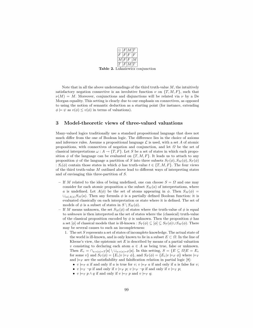
Printed by Dutta Printer, 5 Raja S.C. Mullick Road, Kolkata-700032, India
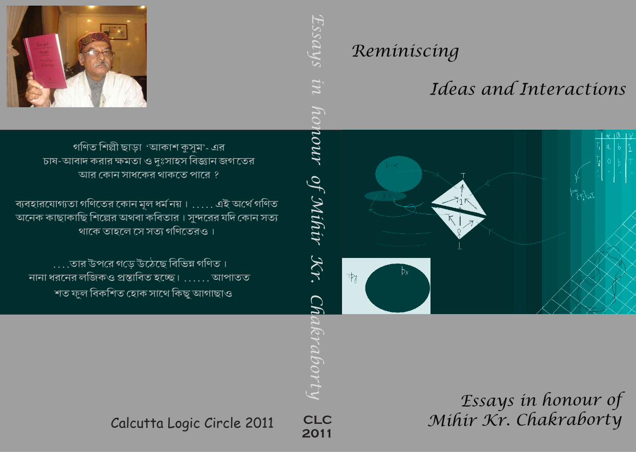
Cover designed by Soma Dutta and Supriya Pahari
Quotations on the back cover are from the following articles in books of Bengaliessays written by Mihir Kr. Chakraborty.
giNt iS°p qaa : Mihir Chakraborty, Akaskusumer Adhikar, in Gan. iterDharapat O Galpasalpa, Nandimukh Samsad, Kolkata, India, 2005, p. 15.
bYbHareJagYta giNetr ekan : Mihir Chakraborty, Sundarer Satya, Gan. iter Satya,in Amimam. sar Alo-Andhari, Nandimukh Samsad, Kolkata, India, 2010, p. 111-112.
tar Uper ge : Mihir Chakraborty, Gan. itjagate Parbaparibartan, inGan. iter Dharapat O Galpasalpa, Nandimukh Samsad, Kolkata, 2005, p. 33.
Sketch on the right by Mihir Kr. Chakraborty (courtesy: Soma Dutta)
KEEP THE FLAG FLYING
(To Professor Mihir K. Chakraborty: An Appreciation)
Haragauri N. Gupta
I was very pleased to receive an invitation to write for a volume of essays in honour of Professor Mihir K. Chakraborty. I have had the privilege of knowing Professor Chakraborty for over thirty five years and take this opportunity to send an appreciation of his work in Logic and his service in the area of Logical research. Mihir K. Chakraborty’s contributions in Logic are considerable. His dedication to Logic is an abiding source of inspiration for his students and has resulted in the creation of the Calcutta Logic Circle (CLC) some twenty five years ago. Members of the circle belong to diverse disciplines. Under Professor Chakraborty’s leadership they gather together to discuss problems arising in their fields, specifically problems of a logical nature. “Logic has been esteemed as the lamp of all studies, the source of all actions and the shelter of all virtues” to quote the ancient Indian savant Kautilya of the third century BC. Modern Logic provides a space where Arts (Humanities), Sciences and Technology interplay to the mutual benefit of them all. It also gives valuable insights for Philosophy, Mathematics, Computer Science, Engineering, and Linguistics, to name only a few. The growth of Logic in recent times is astounding. For about two thousand years since Aristotle (384-324 BC) Logic remained in the shape which Aristotle gave to it. Then, about the middle of the 19th century some mathematicians (Boole, De Morgan, Peirce, and Schroeder et al) began to investigate the logical processes as they existed at the time. They brought to the open the mathematical nature of much that went in the name of Logic. For example, the propositional core of logic was seen to constitute a mathematical system, ushering in the Boolean Algebra. The Aristotelian System of syllogisms was extended to become the Predicate Calculus of today (Frege, Russell, Hilbert). (Why did this much needed generalization have to wait for so long?) Fundamental questions on the newly emerging logical systems were raised and answered using mathematical methods. This was possible because of a parallel event in Mathematics itself, namely, the emergence of Set Theory (Cantor, Dedekind, Zermelo). The concept of truth (at least in formalized languages) was cleared up by Alfred Tarski (1901-1983) putting Logic of derived knowledge on reliable semantic foundations. Model Theory emerged. Notions of completeness, decidability and axiomatizability of theories (mathematical) began to engage the attention of mathematicians. Kurt Godel (1906-1978) made groundbreaking discoveries in Logic and Set Theory. His arithmetization of logical syntax can be perceived as fulfilment of the Leibnizian dream. Way back in the seventeenth century G.W. Leibniz (1646-1716) had advanced the idea that Logic ought to be seen as a variety of Mathematics both in content and in form (calculemos). All this happened in a brief span of time (1840-1930) blurring the
distinction between Mathematics and Logic. Logic is no longer in the exclusive care of philosophers. Doors of cross-fertilization with other disciplines have been flung open. Alternative, non-standard logics have emerged (many-valued logics, modal logics, Logic of fuzzy sets, Logic of rough sets). Computer Science appeared and is growing in rapid strides. We are witness to a magnificent era of cooperation, wondering at the power that interplay of disciplines can generate. Members of the Calcutta Logic Circle are held together by this shared sense of wonder. They welcome everything that can be seen as the logical heart of their concerns. They meet regularly to discuss logical matters. Under Mihir K. Chakraborty’s leadership, the Calcutta Logic Circle has brought about a renaissance of logical studies in Calcutta and beyond. The present volume of essays is a fitting testimonial to the measure of respect and gratefulness which his students, colleagues and members of the Calcutta Logic Circle feel toward him. It is a lovely way indeed to felicitate a loving and caring teacher. From overseas, I send Mihir Chakraborty warmest good wishes on his sixty fifth birthday and wish him many more years of service to Logic and Learning. To the Calcutta Logic Circle I say:
Keep the Flag Flying
Haragauri N. Gupta Emeritus Professor, Department of Mathematics & Statistics, University of Regina, Canada. [email protected]
Contents
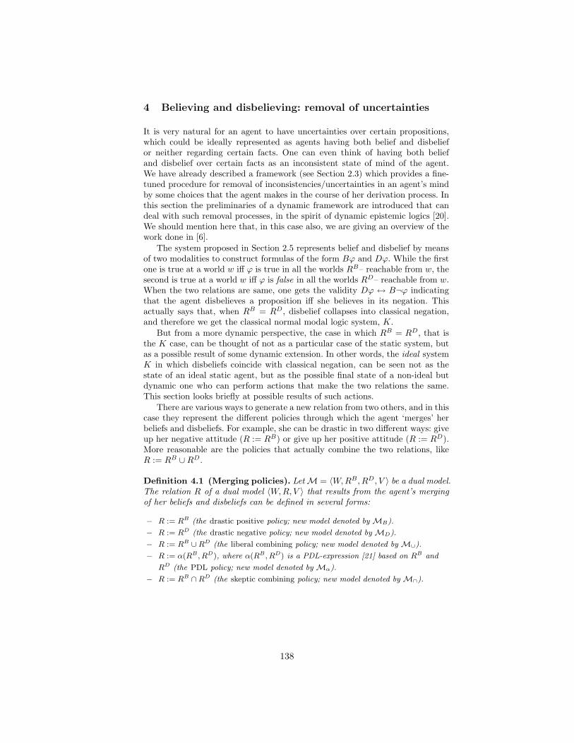
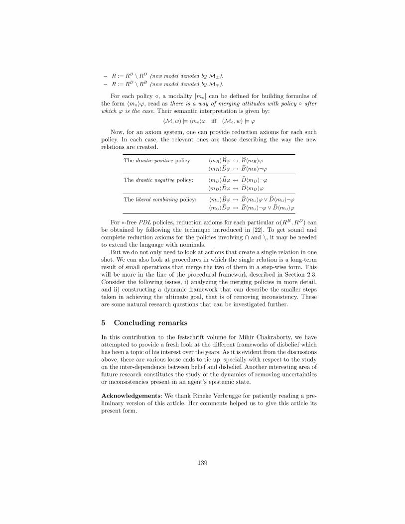
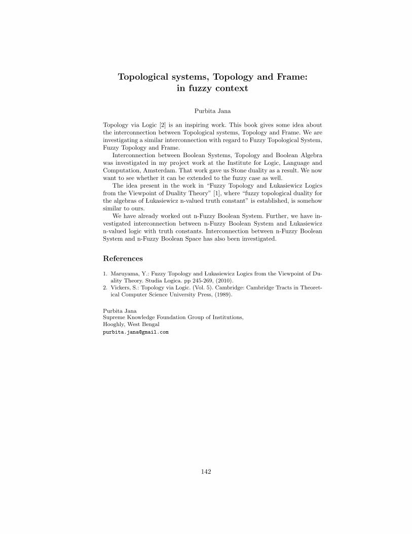
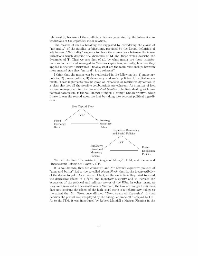
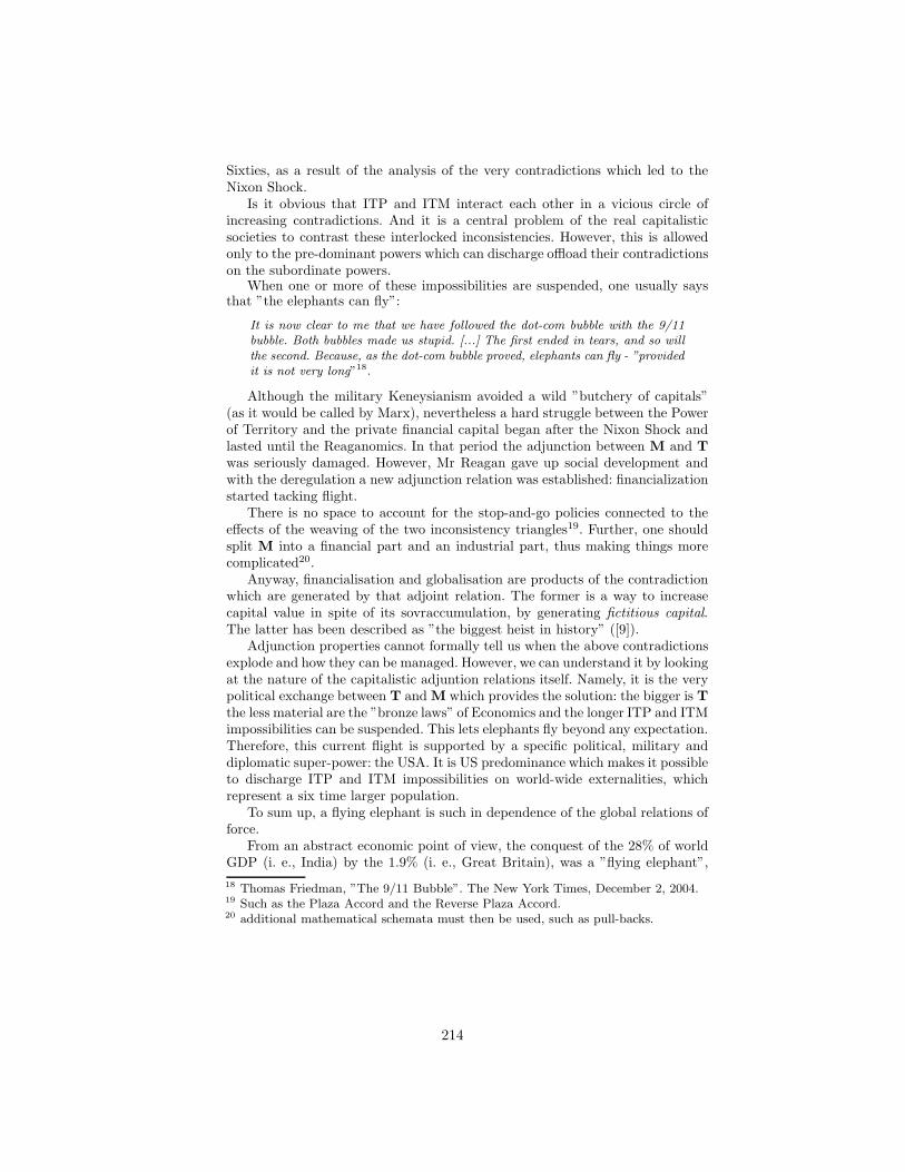
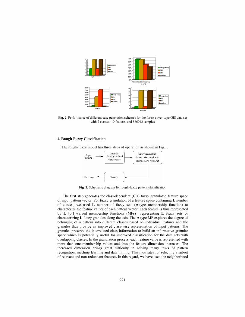
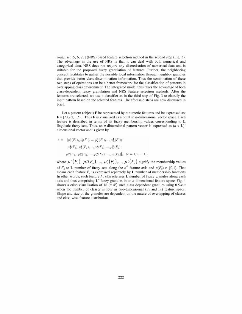
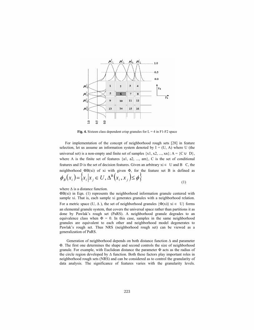
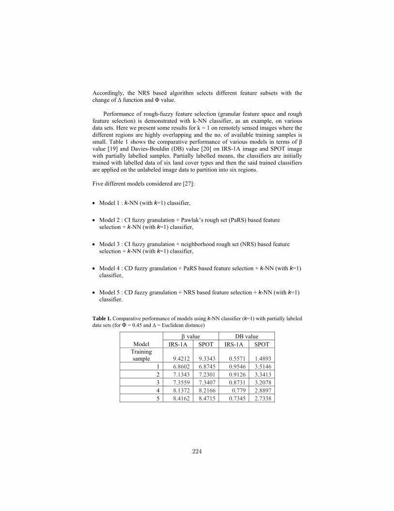
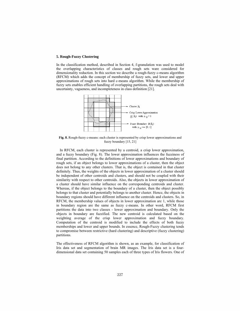
Preface 11Algebraic Studies in Pawlak’s Rough Set TheoryMohua Banerjee 13Should Logic Be Normative?Sanjukta Basu 32Rough Sets and Vague ConceptsJan Bazan, Andrzej Skowron, Jaros law Stepaniuk, Roman Swiniarski 38Enigma of ContradictionLopamudra Choudhury 73Some technical features of the graded consequenceCristina Coppola and Giangiacomo Gerla 80Three-valued logics and Knowledge Representation: Pragmatic IssuesDidier Dubois 95A fragment of Mathematics from graded context: a proposalSoma Dutta 108Belief and disbelief: a logic approachSujata Ghosh 120Topological systems, Topology and Frame: in fuzzy contextPurbita Jana 142Generalizations and Logics of Rough Set TheoryMd. Aquil Khan 143Axioms for locality as productKamal Lodaya and R. Ramanujam 162Jibaner pathe dekha haoya ek ananya byaktitvaMadhabendranath Mitra 181Can the feminists qua feminists be allies of M.C.?Shefali Moitra 184GeneralizingRanjan Mukhopadhyay 193Universality, locality, dialectic, dynamics and contradiction.Logico-political thoughts in honour of professor Mihir K. ChakrabortyPiero Pagliani 196F-granulation and Generalized Rough Sets: Uncertainty analysis andpattern recognitionSankar K. Pal 217The Notion of Consistency in the Presence of Knowledge OperatorSaswati Sadhu 239
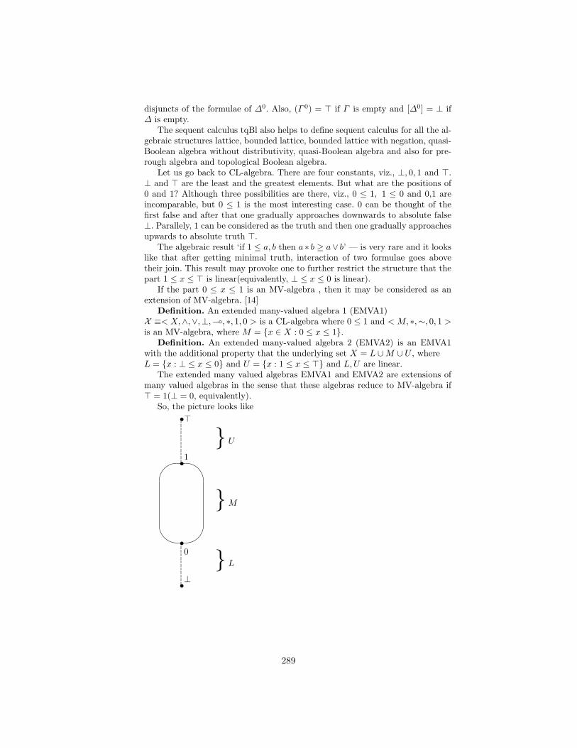
Axiomatization of Topological Quasi Boolean AlgebraAnirban Saha 244Generalized Rough Sets, Implication Lattices andConsistency-DegreePulak Samanta 247Journey and Joy of MathematicsSatyabachi Sar 263Mathematics and music: An aesthetic detour into logicSundar Sarukkai 270Contractifiability and Equivalent MetricesAmita Sen 278A glimpse of linear logic and its algebraJayanta Sen 283Some aspects of Fuzzy Hyperstructure TheoryM.K. Sen 292The Nature of ANUMEYA: Some Early Indian ViewsPrabal Kumar Sen 304Some Musings on Mathematical Creations and RationalitySmita Sirker 312Some pages from my diarySourav Tarafder 322
Preface
It was in 1985 when a mathematician in love with logic invited one of his teachersHaragauri Narayan Gupta, a prominent student of Alfred Tarski, to deliver acourse of lectures designed for charting a roadmap for serious studies in logic athis workplace, the University of Calcutta, Kolkata. A motley collection of peoplealso interested in logic, but from various disciplines, gathered to go through thecourse. The course ended, but the craving for more and more of what was servedwas felt by the mathematician, and, encouraged by the mood of the othersaround him, he took up the challenging task of forming a community of logiclovers single handedly, providing the infrastructure, the planning and also theresources in terms of materials and seminars, all by himself. The community,although informal, bonded slowly into a close knit group, the cementing factorbeing the gentle yet irresistible personality of Mihir Kumar Chakraborty, themathematician we have been talking about.
The community, called Calcutta Logic Circle, is still alive, informally. Frominitially being a study group, it has now become a research group gaining theaffection, attention and support of many around the country and abroad. In itsjourney many have joined, and some have drifted away, but a core group – not allof them residing in Kolkata – remains, keeping in touch with all those who carefor it. The central figure, around whom all in the group assembled sometime orother, called variously as MKC, Mihirda, Mihirbabu, Mihir, Sir, etc. (dependingon the context and relationship), turns sixty five this year. It is not only in ashow of respect for this person – an extra-ordinary teacher – but also in a showof solidarity with the ideas, vision and efforts of his in letting this communitylive, that Calcutta Logic Circle presents a collection of essays on the occasion(prepared as a surprise for him).
A variety of articles, touching various aspects of his life and philosophy,and ranging from technical articles on different areas of logic and mathematicsthat he has worked on, to very personal ones, written by his students, friends,colleagues and members of Calcutta Logic Circle, give this volume a uniquelook. We hope that, through these articles, the readers would get a glimpse ofhis vision and ideas, as well as of him as a person. A few of his graduate studentshave presented outlines of their ongoing doctoral work, thus giving an idea ofhis current research projects as well.
We are indebted to Haragauri Narayan Gupta for supporting our effort whole-heartedly and contributing to this volume. Our sincere thanks go to all the otherauthors, who have unhesitatingly given their consent to contribute, and thenvaluable time and effort in preparing the articles. The members of CalcuttaLogic Circle also thank their family, friends and colleagues for providing themuch needed support in making this volume a reality.
Calcutta Logic Circle, 2011
http://home.iitk.ac.in/∼mohua/CLC.html
11
Algebraic Studies in Pawlak’s Rough Set Theory
Mohua Banerjee
1 Introduction
Indiscernibility has been at the focus of debates, for ages. I ventured to makeit the focus of my Ph.D. thesis [1] as well, spurred on by my supervisor’s veryinfectious enthusiasm1 about the notion. We explored it from different points ofview, which led to the consideration of different approximate identities. In par-ticular, we considered the situation when there was lack of complete informationon the objects of the domain involved – which is just what Pawlak’s rough settheory [31] deals with. The theory hinges on the notion of an approximationspace (U,R), where R is an indiscernibility relation on the domain of discourseU , represented by a partition.
Since the interest in the thesis was on foundational issues, we naturally tooka close look at operations on rough sets. Pawlak had, of course, meticulouslylisted some immediate properties, in his first paper itself, and later in his book[32]. However, that was clearly only a starting point, and not surprisingly, soonafter, questions on algebras that could be formed with rough sets as basic entitiessurfaced, and started being addressed by many. We joined the bandwagon, soto speak, but soon realized that we must put the study in perspective. Theresult turned out to be a list of algebras, both new and well-known, the commonfeature being that each has a ‘rough set’ as an instance. In this article, wepresent an account of the developments in the study of algebraic structures thatresult only from ‘classical’ rough set theory, i.e. ones using notions defined byPawlak. There have also been algebraic investigations in various generalizationsof rough set theory, but covering those is beyond the scope of this article. A briefpresentation of these studies is made at the end in [6]. The account presentedhere is a re-organized and updated version of that in [6]. We also refer to [23].
In order to develop an algebra an instance (or model) of which would be roughsets, it is clearly necessary to specify the definition of a rough set. Interestingly,we find that there are four set-based definitions of a (Pawlak) rough set itself,viz. Definitions 3, 4, 5, 6 below. Apart from these, we also have the ‘operator-oriented’ view [37] reflected by Definitions 1, 2.
First, a brief on the preliminaries [32]. Consider an approximation space(U,R). Let [x] denote the equivalence class of the element x of U under theequivalence relation R. For any subset A of U , the lower approximation A ofA in the approximation space (U,R) is the set x ∈ U : [x] ⊆ U, i.e. theunion of equivalence classes contained in A. The upper approximation A of A in1 This is only one amongst various other subjects, mostly non-standard, many “non-
academic”, that Prof. Mihir Chakraborty continues to inspire me about, in quite asimilar manner.
13
(U,R) is the set x ∈ U : [x]∩A 6= ∅: the union of equivalence classes properlyintersecting A. The boundary BnA of A is the set A \A – it consists of elementspossibly, but not definitely, in A. A definable set in (U,R) is one whose boundaryis empty.Two sets A,B in (U,R) are said to be roughly equal, denoted A ≈ B, providedA = B, as well as A = B. ≈, clearly is an equivalence relation on P(U), thepower set of U .
Definition 1. [32] A ⊆ U is a rough set in (U,R), provided Bn(A) 6= ∅.
For generality’s sake however, we could remove the restriction in the definitionabove, and term any subset A of U rough. A definable set then becomes a specialcase of a rough set. Moreover, to keep the context clear, we could have
Definition 2. The triple (U,R,A) is called a rough set [3].
Definition 3. (cf. [23]) The pair (A,A), for each A ⊆ U , is called a rough setin (U,R).
Definition 4. [29] The pair (A,Ac), for each A ⊆ U , is called a rough set in
(U,R), where c denotes complementation in P(U).
Definition 5. [27] Given an approximation space (U,R), a rough set is an or-dered quadruple (U,R,L,B), where (i) L,B are disjoint subsets of U , (ii) bothL and B are definable sets in (U,R), and (iii) for each x ∈ B there exists y ∈ Bsuch that x 6= y and xRy (i.e. no equivalence class contained in B is a singleton).
Definition 6. [31] A rough set in (U,R) is an equivalence class of P(U)/ ≈.
Let us fix an approximation space (U,R). We denote by Fi, i = 1, . . . , 5, thecollection of all rough sets corresponding to (U,R), given by Definition 1, 3, 4,5, 6 respectively, only the version of Definition 5 where (U,R) is fixed in all thequadruples, is considered to get F4. We observe that Definitions 3, 4, 5 and 6 areequivalent to each other for any given (U,R), in the sense that there is a one-onecorrespondence between families F2, F3, F4 and F5. Indeed, for any A ⊆ U ,the entities (A,A), (A,A
c) and the equivalence class [A] of A in P(U)/ ≈ are
identifiable. Again, for a fixed (U,R), a quadruple (U,R,L,B) is essentially thepair (L,B), and due to condition (iii) of Definition 5, one can always find asubset A of U such that A = L and Bn(A) = B. Hence Definition 5 may bereformulated as follows: the pair (A,Bn(A)) for each A ⊆ U is a rough set solong as (U,R) remains unchanged. So, via this interpretation, Definition 5 alsobecomes equivalent to 3, 4 and 6. These definitions have been said to representthe ‘set-oriented’ view of rough sets, viz. when rough sets are defined throughpairs of definable sets. In contrast, Definitions 1 and 2 are said to represent the‘operator-oriented’ view, where the term ‘rough’ is used as an adjective for thesubset A of U , and operators of lower and upper approximations are defined onU , in order to approximately describe A.
14
However, as we shall see in this article, these equivalent definitions yielddifferent (though related) algebras, by taking different definitions of union, in-tersection, complementation and other algebraic operations.
Apart from the above families F1, . . . ,F5, another collection that makes anappearance in the algebraic studies is R := (D1, D2), D1 ⊆ D2, D1, D2 ∈ D,where D denotes the collection of all definable sets of a fixed approximation space(U,R).Notice that R is a generalization of F2 : F2 ⊆ R. Further, since D2 \D1 mayinclude singleton equivalence classes, F2 may be a proper subset of R.
A summary of the structures obtained by considering the families aboveare presented in Section 2. Section 3 presents the algebras obtained from theoperator-based definitions, that include ones coming from information systems,another basic notion in rough set theory. Both Sections 2 and 3 give the mainresults proved about the algebras as well. In Section 4, we outline the variousrelationships that are obtained among these algebras. Section 5 concludes thearticle.
2 Algebras from set-based definitions
One finds that the different algebras emerging from the set-based definitions ofrough sets are instances of :
3. regular double Stone algebras [15, 29];4. complete atomic Stone algebras [12];5. semi-simple Nelson algebras [29];6. 3-valued Lukasiewicz algebras [29, 18].
In the sequel, we sketch how exactly these algebras come about, startingfrom the definitions of rough sets. Broadly, the scheme is of the following nature.As remarked in the Introduction, the primary task is to fix the definition of arough set and therefore the corresponding family. The next step is to take anappropriate operation of union / intersection / complementation / interior etc.on the family, to give rise to a class of algebraic structures, sayRS. This leads, onabstraction (according to the properties of the operations in RS), to one of theclasses of algebras in the preceding list. In many cases, the connection betweenRS and the corresponding class (say A) of abstract algebras, is formalized byestablishing a representation result. One demonstrates a correspondence c : A →RS such that any element A ∈ A is isomorphic to a subalgebra of c(A). In somecases, a reverse representation is proved.
We note that when the family F2, or the more general R is considered, anatural definition for the operations of union and intersection of the memberswould be the following.
15
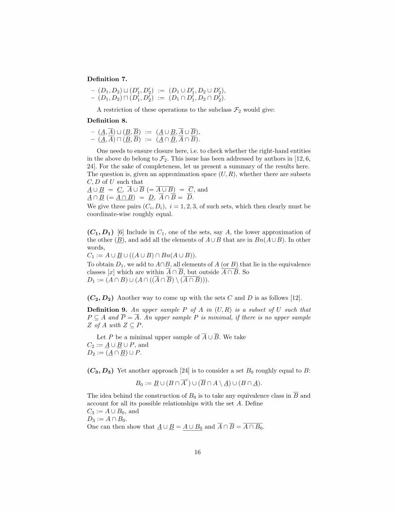
Definition 7.
– (D1, D2) t (D′1, D′2) := (D1 ∪D′1, D2 ∪D′2),
– (D1, D2) u (D′1, D′2) := (D1 ∩D′1, D2 ∩D′2).
A restriction of these operations to the subclass F2 would give:
Definition 8.
– (A,A) t (B,B) := (A ∪B,A ∪B),– (A,A) u (B,B) := (A ∩B,A ∩B).
One needs to ensure closure here, i.e. to check whether the right-hand entitiesin the above do belong to F2. This issue has been addressed by authors in [12, 6,24]. For the sake of completeness, let us present a summary of the results here.The question is, given an approximation space (U,R), whether there are subsetsC,D of U such thatA ∪B = C, A ∪B (= A ∪B) = C, andA ∩B (= A ∩B) = D, A ∩B = D.We give three pairs (Ci, Di), i = 1, 2, 3, of such sets, which then clearly must becoordinate-wise roughly equal.
(C1, D1) [6] Include in C1, one of the sets, say A, the lower approximation ofthe other (B), and add all the elements of A∪B that are in Bn(A∪B). In otherwords,C1 := A ∪B ∪ ((A ∪B) ∩Bn(A ∪B)).To obtain D1, we add to A∩B, all elements of A (or B) that lie in the equivalenceclasses [x] which are within A ∩B, but outside A ∩B. SoD1 := (A ∩B) ∪ (A ∩ ((A ∩B) \ (A ∩B))).
(C2, D2) Another way to come up with the sets C and D is as follows [12].
Definition 9. An upper sample P of A in (U,R) is a subset of U such thatP ⊆ A and P = A. An upper sample P is minimal, if there is no upper sampleZ of A with Z ⊆ P .
Let P be a minimal upper sample of A ∪B. We takeC2 := A ∪B ∪ P , andD2 := (A ∩B) ∪ P .
(C3, D3) Yet another approach [24] is to consider a set B0 roughly equal to B:
B0 := B ∪ (B ∩Ac) ∪ (B ∩A \A) ∪ (B ∩A).
The idea behind the construction of B0 is to take any equivalence class in B andaccount for all its possible relationships with the set A. DefineC3 := A ∪B0, andD3 := A ∩B0.One can then show that A ∪B = A ∪B0 and A ∩B = A ∩B0.
16
2.1 Quasi-Boolean algebras
Definition 10. [35] A quasi-Boolean algebra (or a De Morgan lattice) is abounded distributive lattice (A,≤,∨,∧, 0, 1) with a unary operation ¬ that satis-fies involution (¬¬a = a, for each a ∈ A), and makes the De Morgan identitieshold.
Iwinski [19] and Pomyka la [33] show that rough sets form structures thatare quasi-Boolean algebras. Iwinski, presenting a ‘rough algebra’ for the firsttime, follows Definition 3. The general collection R instead of F2 is considered.Operations of join (t) and meet (u) on R are given by Definition 7. It may benoted that any definable set A of (U,R) is identifiable with the pair (A,A) ofR. Further,
Definition 11. ¬(D1, D2) := (D2c, D1
c), where c denotes ordinary set-theoreticcomplementation.
¬ satisfies the De Morgan identities, and when restricted to definable sets, is theusual complement. But it does not satisfy the laws of Boolean complementationin general.
Proposition 1. [19] (R,t,u,¬, 0, 1) is a complete atomic quasi-Boolean alge-bra, where 0 := (∅, ∅) and 1 := (U,U). Atoms are of the form (∅, A), A being anelementary set of (U,R). The definable sets form a maximal Boolean subalgebraof (R,t,u,¬, 0, 1).
Does the converse of this proposition hold? Let us see.A basic finite quasi-Boolean algebra is U0 := (0, a, b, 1,∨,∧,¬, 1). It is adiamond as a lattice, viz.
1
a b
0and ¬ is given by the equations :
¬0 := 1, ¬1 := 0, ¬a := a, ¬b := b.It is known [35] that any quasi-Boolean algebra is isomorphic to a subalgebra ofthe product
∏i∈I Ui, where I is a set of indices, and Ui = U0.
Hence, to address the converse of proposition 1, it seems natural to askif U0 is isomorphic to some R. The answer is in the negative, since for anymember (D1, D2) of R other than (∅, X), ¬(D1, D2) 6= (D1, D2), whereas in U0,¬a = a, ¬b = b and a 6= b. So the class R is a proper subclass of the class ofquasi-Boolean algebras.
No representation result is proved in [19]. However, if one considers the familyF2, such a result is obtained in [33].
Clearly, (F2,t,u,¬, 0, 1) is also a quasi-Boolean algebra, the operations beingrestrictions of those in R. But [33] says more. An important notion involved here
17
is that of an ‘individual atom’ – a singleton elementary class. Let us denote byS, the collection of all individual atoms in the approximation space < X,R >.Two simple examples of quasi-Boolean algebras are the two and three elementchains B0 := (0, 1,∨,∧,¬, 1) and C0 := (0, a, 1,∨,∧,¬, 1) respectively.¬ is defined as: ¬0 := 1, ¬1 := 0, ¬a := a.
Theorem 1. (F2,t,u,¬, 0, 1) is isomorphic to a subalgebra of the product∏i∈I Ui, where I is a set of indices, and Ui = B0 or Ui = C0, for each i ∈ I.
It should be mentioned that Pomyka la came up with a number of algebraicstructures that have F2 as domain. These differ from each other with respect tothe complementation and implication operations chosen.
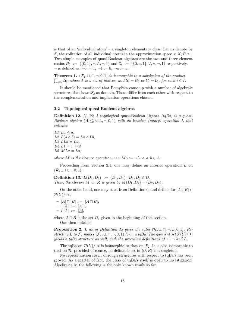
2.2 Topological quasi-Boolean algebras
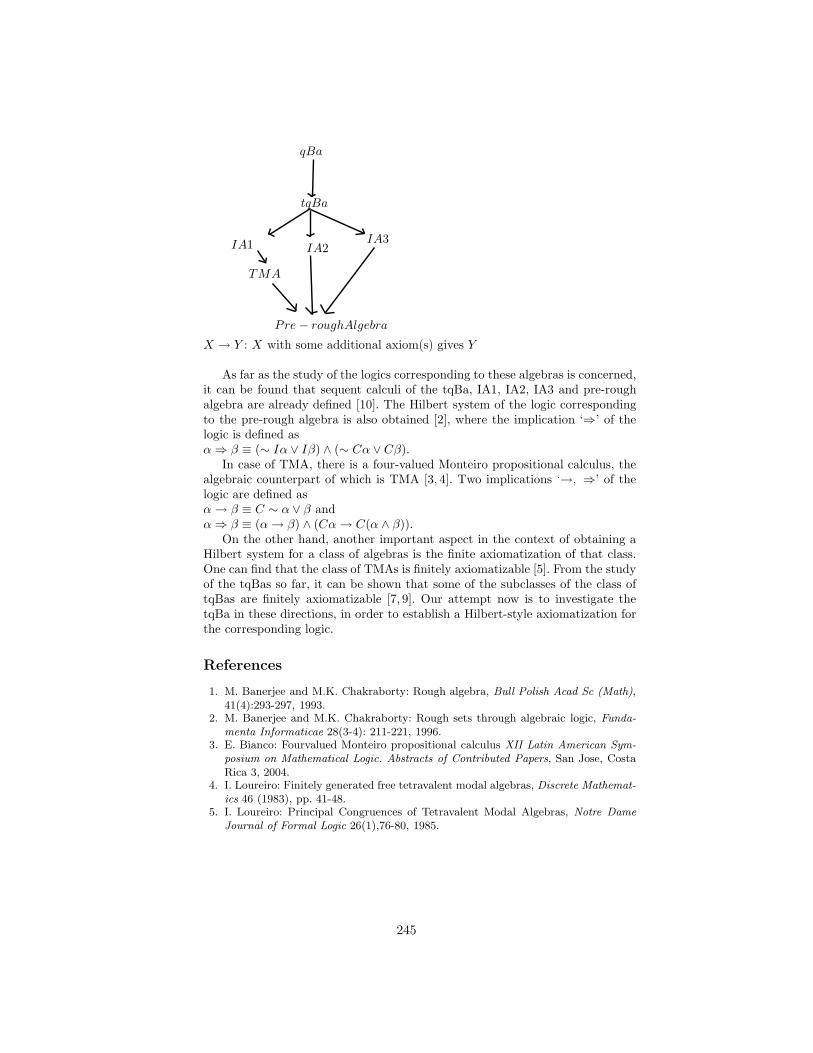
Definition 12. [4, 36] A topological quasi-Boolean algebra (tqBa) is a quasi-Boolean algebra (A,≤,∨,∧,¬, 0, 1) with an interior (unary) operation L thatsatisfies
L1 La ≤ a,L2 L(a ∧ b) = La ∧ Lb,L3 LLa = La,L4 L1 = 1 andL5 MLa = La,
where M is the closure operation, viz. Ma := ¬L¬a, a, b ∈ A.Proceeding from Section 2.1, one may define an interior operation L on
(R,t,u,¬, 0, 1):
Definition 13. L(D1, D2) := (D1, D1), D1, D2 ∈ D.Thus, the closure M on R is given by M(D1, D2) = (D2, D2).
On the other hand, one may start from Definition 6, and define, for [A], [B] ∈P(U)/ ≈,
where A uB is the set D1 given in the beginning of this section.One then obtains
Proposition 2. L as in Definition 13 gives the tqBa (R,t,u,¬, L, 0, 1). Re-stricting L to F2 makes (F2,t,u,¬, 0, 1) form a tqBa. The quotient set P(U)/ ≈yields a tqBa structure as well, with the preceding definitions of u,¬ and L.
The tqBa on P(U)/ ≈ is isomorphic to that on F2. It is also isomorphic tothat on R, provided of course, no definable set in (U,R) is a singleton.
No representation result of rough structures with respect to tqBa’s has beenproved. As a matter of fact, the class of tqBa’s itself is open to investigation.Algebraically, the following is the only known result so far.
18
Proposition 3. [8] TqBa’s form a variety that is not a discriminator variety.
The tqBas on P(U)/ ≈ and F2 satisfy more properties, as we shall see inSections 2.3 and 2.4.
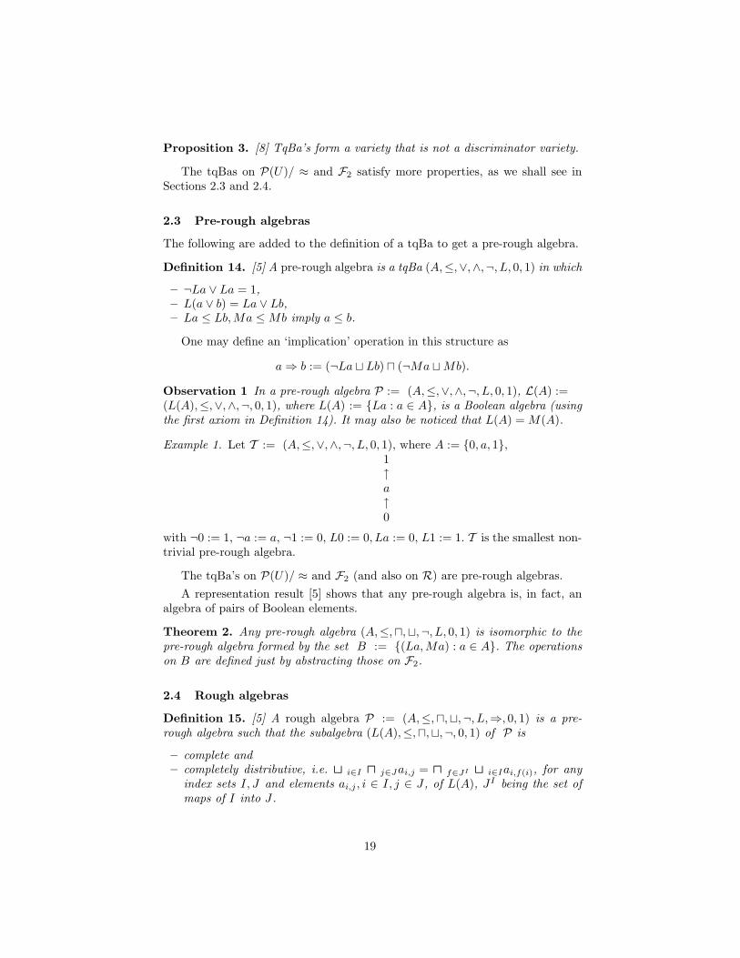
2.3 Pre-rough algebras
The following are added to the definition of a tqBa to get a pre-rough algebra.
Definition 14. [5] A pre-rough algebra is a tqBa (A,≤,∨,∧,¬, L, 0, 1) in which
– ¬La ∨ La = 1,– L(a ∨ b) = La ∨ Lb,– La ≤ Lb,Ma ≤Mb imply a ≤ b.
One may define an ‘implication’ operation in this structure as
a⇒ b := (¬La t Lb) u (¬Ma tMb).
Observation 1 In a pre-rough algebra P := (A,≤,∨,∧,¬, L, 0, 1), L(A) :=(L(A),≤,∨,∧,¬, 0, 1), where L(A) := La : a ∈ A, is a Boolean algebra (usingthe first axiom in Definition 14). It may also be noticed that L(A) = M(A).
Example 1. Let T := (A,≤,∨,∧,¬, L, 0, 1), where A := 0, a, 1,1↑a↑0
with ¬0 := 1, ¬a := a, ¬1 := 0, L0 := 0, La := 0, L1 := 1. T is the smallest non-trivial pre-rough algebra.
The tqBa’s on P(U)/ ≈ and F2 (and also on R) are pre-rough algebras.A representation result [5] shows that any pre-rough algebra is, in fact, an
algebra of pairs of Boolean elements.
Theorem 2. Any pre-rough algebra (A,≤,u,t,¬, L, 0, 1) is isomorphic to thepre-rough algebra formed by the set B := (La,Ma) : a ∈ A. The operationson B are defined just by abstracting those on F2.
2.4 Rough algebras
Definition 15. [5] A rough algebra P := (A,≤,u,t,¬, L,⇒, 0, 1) is a pre-rough algebra such that the subalgebra (L(A),≤,u,t,¬, 0, 1) of P is
– complete and– completely distributive, i.e. t i∈I u j∈Jai,j = u f∈JI t i∈Iai,f(i), for any
index sets I, J and elements ai,j , i ∈ I, j ∈ J , of L(A), JI being the set ofmaps of I into J .
19
The pre-rough algebras on each of P(U)/ ≈, F2 and R, are rough algebrasas well. The following representation result is then obtained.
Theorem 3. Any rough algebra is isomorphic to a subalgebra of(R,t,u,¬, L, 0, 1) corresponding to some approximation space (U,R).
In fact, one can show [6] that
Corollary 1. Any rough algebra is isomorphic to a subalgebra of P(U ′)/ ≈ forsome approximation space (U ′, R′).
2.5 Complete atomic Stone algebras
Definition 16. A Stone algebra is a bounded distributive lattice (A,≤,∨,∧, 0, 1)which has a pseudo-complement ∗ on A, i.e. y ≤ x∗ if and only if y ∧ x = 0,and which satisfies the Stone identity, viz. x∗ ∨ x∗∗ = 1.
In [34], Pomyka la defines ∗ on F2 as:
Definition 17. (A,A)∗ := (Ac, A
c), (A,A) ∈ F2.
Then one obtains (with t,u as in Definition 8, and 0, 1 as in Proposition 1)
Proposition 4. (F2,t,u,∗ , 0, 1) is a Stone algebra.
However, no representation is obtained.Starting from Definition 6, [12] arrives at an enhanced rough structure.
(P(U)/ ≈,≤) is clearly a partially ordered set, ≤ being defined in terms of roughinclusion, i.e. [A] ≤ [B], if and only if A is roughly included in B, [A], [B] ∈P(U)/ ≈. Now operations of join (∪≈), meet (∩≈) on P(U)/ ≈ and (‘exterior’)complementation (ex) are defined.
For a subset A of U , an upper sample P is such that P ⊆ A and P = A. Anupper sample P of A is minimal, if there is no upper sample Z of A with Z ⊆ P .Then
Definition 18. – [A] ∪≈ [B] := [A ∪ B ∪ P ], where P is a minimal uppersample of A ∪B, and
– [A]∩≈ [B] := [(A∩B)∪P ], where P is a minimal upper sample of A∩B.– [A]ex := [(A)c].
One may note that ∅ is included among elementary sets. For a finite domain U ,
Proposition 5. (P(U)/ ≈,∪≈,∩≈,ex , [∅], [U ]) is a complete atomic Stone alge-bra, where the atoms are determined by proper subsets of the elementary sets orby singleton elementary sets in (U,R).
Again, no representation is obtained. Such a result is found though, on in-troducing a further operation on the family of rough sets F2.
20
2.6 Regular double Stone algebras
Definition 19. A double Stone algebra (dSa) is a Stone algebra (A,∨,∧,∗ , 0, 1)which has a dual pseudo-complement +, i.e.
– y ≥ x+ if and only if y ∨ x = 1,
and which satisfies
– x+ ∧ x++ = 0.
The dSa is regular if, for all x, y ∈ A,
– x ∧ x+ ≤ y ∨ y∗ holds.
(This is equivalent to requiring that
– x∗ = y∗, x+ = y+ imply x = y, for all x, y ∈ A.)
[15] introduces a dual pseudo-complementation + on F2 and gets, further toProposition 4,
Proposition 6. (F2,t,u,∗ ,+ , 0, 1), for a given approximation space (U,R), isa regular dSa, where (A,A)+ := (Ac, Ac).
As a representation result, Comer obtains
Theorem 4. Any regular dSa is isomorphic to a subalgebra of(F2,t,u,∗ ,+ , 0, 1) for some approximation space (U,R).
2.7 Semi-simple Nelson algebras
Definition 20. [35] A Nelson algebra is a quasi-Boolean algebra (A,∧,∨,¬, 0, 1)equipped with a unary operation ∼ and a binary operation → such that, for anya, b, x ∈ A,
– a ∧ ¬a ≤ b ∨ ¬b,– a ∧ x ≤ ¬a ∨ b if and only if x ≤ a→ b,– a→ (b→ c) = (a ∧ b)→ c,– ∼ a = a→ ¬a = a→ 0.
A Nelson algebra A is semi-simple, if a ∨ ∼ a = 1, for all a ∈ A.
¬ and ∼ are the ‘strong’ and ‘weak’ negations on A respectively.These algebras are discussed in the context of rough sets in [29], which con-
siders finite domains, and adopts Definition 4. It is observed that
Proposition 7. (F3,u,t,¬,∼,→, 0, 1) is a semi-simple Nelson algebra, the op-erations being defined as:
– (A1, A1c) u (A2, A2
c) := (A1 ∩A2, A1
c ∪A2c),
21
– (A1, A1c) t (A2, A2
c) := (A1 ∪A2, A1
c ∩A2c),
– (A1, A1c)→ (A2, A2
c) := (A1
c ∪A2, A1 ∩A2c),
– ¬(A1, A1c) := (A1
c, A1), and
– ∼ (A1, A1c) := (A1
c, A1).
The representation theorem is as follows.
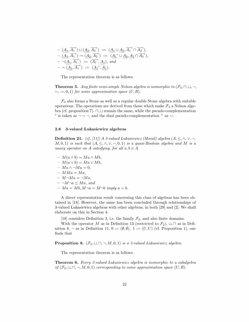
Theorem 5. Any finite semi-simple Nelson algebra is isomorphic to (F3,u,t,¬,∼,→, 0, 1) for some approximation space (U,R).
F3 also forms a Stone as well as a regular double Stone algebra with suitableoperations. The operations are derived from those which make F3 a Nelson alge-bra (cf. proposition 7). u,t remain the same, while the pseudo-complementation∗ is taken as ¬ ∼ ¬, and the dual pseudo-complementation + as ∼.
2.8 3-valued Lukasiewicz algebras
Definition 21. (cf. [11]) A 3-valued Lukasiewicz (Moisil) algebra (A,≤,∧,∨,¬,M, 0, 1) is such that (A,≤,∧,∨,¬, 0, 1) is a quasi-Boolean algebra and M is aunary operator on A satisfying, for all a, b ∈ A
– M(a ∧ b) = Ma ∧Mb,– M(a ∨ b) = Ma ∨Mb,– Ma ∧ ¬Ma = 0,– MMa = Ma,– M¬Ma = ¬Ma,– ¬M¬a ≤Ma, and– Ma = Mb,M¬a = M¬b imply a = b.
A direct representation result concerning this class of algebras has been ob-tained in [18]. However, the same has been concluded through relationships of3-valued Lukasiewicz algebras with other algebras, in both [29] and [2]. We shallelaborate on this in Section 4.
[18] considers Definition 3, i.e. the family F2, and also finite domains.With the operator M as in Definition 13 (restricted to F2), t,u as in Defi-
nition 8, ¬ as in Definition 11, 0 := (∅, ∅), 1 := (U,U) (cf. Proposition 1), onefinds that
Proposition 8. (F2,t,u,¬,M, 0, 1) is a 3-valued Lukasiewicz algebra.
The representation theorem is as follows.
Theorem 6. Every 3-valued Lukasiewicz algebra is isomorphic to a subalgebraof (F2,t,u,¬,M, 0, 1) corresponding to some approximation space (U,R).
22
2.9 Other algebras
In the special situation when the approximation space has no singleton elemen-tary sets in it, [29] observes that F2 with its pairs in reverse order, viz. thecollection of pairs (A,A), A ⊆ U , turns out to be a Post algebra of order three[35]. Therefore [13], it is a 3-valued Lukasiewicz algebra with a centre (i.e. anelement c such that ¬c = c).
In the general situation (with no restriction on the approximation space), thesame structure can be made into an algebra that is a generalization of a Postalgebra, viz. a certain chain-based lattice of order three [16].
3 Algebras from operator-based definitions
As mentioned in the Introduction, in the operator-oriented approach, the lowerand upper approximations are viewed as unary operators on the domain. In thesimplest manifestation here, we see that rough set structures form instances ofBoolean algebras with operators.
3.1 Boolean algebras with operators
Definition 22. (cf. [10]) A Boolean algebra with operators is a Boolean algebra(A,∨,∧,∼, 0, 1, ) along with a collection fii∈I of operators on A, where I isan index set. Each n-ary operator fi, i ∈ I, satisfies the two following properties:
An instance of a Boolean algebra with operators, is a topological Booleanalgebra:
Definition 23. [35] A topological Boolean algebra (tBa) is a Boolean algebra(A,∨,∧,∼, 0, 1), that has a unary operation L satisfying the properties L1-L4 ofan interior given in Definition 12.
If (U,R) is an approximation space, the set P(U) of all subsets of U formsa topological Boolean algebra. The interior operation on P(U) is nothing butthe lower approximation with respect to the approximation space (U,R), re-garded as a unary operator on U , i.e. L(X) := X, for any X ⊆ U . L, in fact,satisfies all the properties L1-L5 of Definition 12. The upper approximationoperator, denoted by − say, would then satisfy the properties of a closure oper-ator, which include O1, O2 of Definition 22. In other words, as observed in [18],(P(U),∪,∩,c ,− , ∅, U) forms a monadic Boolean algebra [25], that is an instanceof a Boolean algebra with the single binary operator −. In [38], the lower approx-imation operator , dual to −, is also brought into the picture. Yao studies anabstraction of (P(U),∪,∩,c , ,− ), and considers a structure (P(U),∪,∩,c , L,H),called a rough set algebra. (P(U),∪,∩,c , H) is first taken to be simply a Booleanalgebra with the operator H, and L as an operation on P(U) dual to H. Theresult of imposing further conditions on the two operators are then investigated.
23
3.2 Algebras from complete information systems
A basic notion in rough set theory is that of an information system [31]: a tableproviding information about the values that objects of a domain are assignedunder a given set of attributes.
Definition 24. A complete information system (CIS) S := (U,A,⋃a∈A Va, f),comprises a non-empty set U of objects, A of attributes, Va of attribute-valuesfor each a ∈ A, and information function f : U × A → ⋃
a∈A Va such thatf(x, a) ∈ Va.
Any subset B of the attribute set A induces an indiscernibility relation IndSB(an equivalence relation on U):
(x, y) ∈ IndSB , if and only if f(x, a) = f(y, a) for all a ∈ B.
Each relation IndSB induces an upper approximation operator IndSB on P(U),mapping a set X(⊆ U) to XIndSB
. Similarly, we have a lower approximationoperator IndSB , for each B ⊆ A.
3.2.1 Cylindric algebras
The structure BS := (P(U),∪,∩,c , IndSBB⊆A, ∅, U), is called a knowledge ap-proximation algebra of type A derived from the CIS S in [14]. For each B ⊆ A,the structure (P(U),∪,∩,c , IndSB , ∅, U) is called the (upper) approximation clo-sure algebra of B. It may be noted that this is an instance of a monadic Booleanalgebra.
Now (P(U),∪,∩,c , ∅, U) is not only a Boolean algebra, as mentioned in Sec-tion 3.1, it is also complete, and atomic. In fact, Comer observes that a knowledgeapproximation algebra of type A is an instance of a general algebraic structure,an abstract knowledge approximation algebra of type A.
Definition 25. An abstract knowledge approximation algebra of type A con-sists of a complete atomic Boolean algebra (S,∨,∧,∼, 0, 1), and a family of func-tions KB : S → S, B ⊆ A, A being a finite set. Moreover, the functions satisfythe following, for x, y ∈ S and B,C ⊆ A.
– KB(0) = 0.– KB(x) ≥ x.– KB(x ∧KB(y)) = KB(x) ∧KB(y).– If x 6= 0 then K∅(x) = 1.– KB∪C(x) = KB(x) ∧KC(x), if x is an atom of S.
Comer then indicates the relation of approximation closure algebras withcylindric algebras.
Definition 26. A cylindric algebra of dimension |A| [17] is a structure A :=(U,∧,¬, 0, Λaa∈A, µ(a,b)(a,b)∈A×A), where (U,∧,¬, 0) is a Boolean algebra,and Λa, µ(a,b) are respectively unary and nullary operations on U , such that
24
(L1) Λa(0) = 0,(L2) x ≤ Λa(x),(L3) Λa(x ∧ Λa(y)) = Λa(x) ∧ Λa(y),(L4) Λa(Λb(x)) = Λb(Λa(x)),(L5) µ(a,a) = 1,(L6) If a 6= b, c, then µ(b,c) = Λa(µ(b,a) ∧ µ(a,c)),(L7) If a 6= b, then Λa(µ(a,b) ∧ x) ∧ Λa(µ(a,b) ∧ ¬x) = 0.
We then see that
Proposition 9. Approximation closure algebras are complete atomic cylindricalgebras of dimension one.
A representation theorem is subsequently obtained.
Theorem 7. Every complete atomic cylindric algebra of dimension one is iso-morphic to an approximation closure algebra. In fact, every cylindric algebra ofdimension one is embeddable in an approximation closure algebra.
3.2.2 CIS-algebras
The knowledge approximation algebra derived from a CIS does not give a com-plete description of an information system: attribute and attribute-value pairs,which are the salient features of an information system, do not appear in this de-scription. Thus these algebras are unable to capture the fact that approximationsare induced in information systems by attributes and their values. In a recentwork [22], a class of algebras that takes care of this aspect, has been studied indetail. We give the basic definitions and summary of the results obtained.
In a CIS S := (U,A,⋃a∈A Va, f), we observe that each descriptor [32] (a, v),where a is an attribute, and v an attribute-value, also determines a nullaryoperation (constant) cS(a,v) on P(U):
cS(a,v) := x ∈ U : f(x, a) = v.Let Ω be the tuple (A,V), for a fixed A and V :=
⋃a∈A Va, and let D denote
the set of all descriptors obtained from Ω.
Definition 27. A complete information system algebra (in brief, CIS-algebra)of type Ω generated by a complete information system S := (U,A,V, f) is thestructure
S∗ := (P(U),∩,c , IndSBB⊆A, cSγ γ∈D, ∅).
So a CIS-algebra generated by a CIS S is an extension of the knowledge approx-imation algebra derived from S with a collection of nullary operations.
Making use of some properties that actually turn out to be characterizingproperties of CIS-algebras, a notion of an abstract CIS-algebra is defined.
25
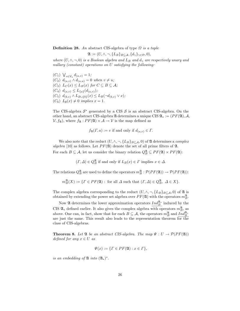
Definition 28. An abstract CIS-algebra of type Ω is a tuple
A := (U,∧,¬, LBB⊆A, dγγ∈D, 0),
where (U,∧,¬, 0) is a Boolean algebra and LB and dγ are respectively unary andnullary (constant) operations on U satisfying the following:
(C1)∨v∈Va
d(a,v) = 1;(C2) d(a,v) ∧ d(a,u) = 0 when v 6= u;(C3) LC(x) ≤ LB(x) for C ⊆ B ⊆ A;(C4) d(a,v) ≤ La(d(a,v));(C5) d(b,v) ∧ LB∪b(x) ≤ LB(¬d(b,v) ∨ x);(C6) L∅(x) 6= 0 implies x = 1.
The CIS-algebra S∗ generated by a CIS S is an abstract CIS-algebra. On theother hand, an abstract CIS-algebra A determines a unique CIS A∗ := (PF (A),A,V, fA), where fA : PF (A)×A → V is the map defined as
fA(Γ, a) := v if and only if d(a,v) ∈ Γ.
We also note that the reduct (U,∧,¬, LBB⊆A, 0) of A determines a complexalgebra [10] as follows. Let PF (A) denote the set of all prime filters of A.
For each B ⊆ A, let us consider the binary relation QAB ⊆ PF (A)× PF (A):
(Γ,∆) ∈ QAB if and only if LB(x) ∈ Γ implies x ∈ ∆.
The relations QAB are used to define the operators mA
B : P(PF (A))→ P(PF (A)):
mAB(X) := Γ ∈ PF (A) : for all ∆ such that (Γ,∆) ∈ QA
B , ∆ ∈ X.
The complex algebra corresponding to the reduct (U,∧,¬, LBB⊆A, 0) of A isobtained by extending the power set algebra over PF (A) with the operators mA
B .
Now A determines the lower approximation operators IndA∗B induced by the
CIS A∗ defined earlier. It also gives the complex algebra with operators mAB , as
above. One can, in fact, show that for each B ⊆ A, the operators mAB and IndA∗
B
are just the same. This result also leads to the representation theorem for theclass of CIS-algebras.
Theorem 8. Let A be an abstract CIS-algebra. The map Ψ : U → P(PF (A))defined for any x ∈ U as
Ψ(x) := Γ ∈ PF (A) : x ∈ Γ,
is an embedding of A into (A∗)∗.
26
4 Relationships
As observed in [29, 6], one can define to and fro transformations to show thatpre-rough, regular double Stone, semi-simple Nelson and 3-valued Lukasiewiczalgebras are all equivalent to each other.
It is not difficult to see that the defining axioms of pre-rough and 3-valued Lukasiewicz algebras (cf. Definitions 14 and 21 respectively), are deducible fromeach other.
The transformations involved for a passage to and from a pre-rough alge-bra (A,∧,∨,¬, L,⇒, 0, 1) and a regular double Stone algebra (Definition 3)(L,∨,∧,∗ ,+ , 0, 1) are:DP1. a+ := ¬La,DP2. a∗ := L(¬a), andPD1. ¬a := (a ∧ a+) ∨ a∗,PD2. La := a++.
For a semi-simple Nelson algebra (Definition 5) N := (A,∧,∨,¬,∼,→, 0, 1)and a pre-rough algebra (A,∧,∨,¬, L,⇒, 0, 1), the transformations are:
NP1. La = ¬ ∼ a,NP2. a⇒ b = ¬ ∼ (a → b),
where a → b := (∼ a∧ ∼ ¬b) ∨ (¬ ∼ ¬a ∨ b), andPN1. ∼ a = ¬La,PN2. a→ b = ¬La ∨ b.
It may be noted that an equivalent axiomatization of 3-valued Lukasiewiczalgebras is given by the Wajsberg algebras.
Definition 29. [11] A Wajsberg algebra is a structure (A,→,¬, 1) such that
1. a→ (b→ a) = 1,2. (a→ b)→ ((b→ c)→ (a→ c)) = 1,3. ((a→ ¬a)→ a)→ a = 1,4. (¬a→ ¬b)→ (b→ a) = 1,5. If 1→ a = 1 then a = 1,6. If a→ b = 1 = b→ a then a = b,
where a, b, c ∈ A.
Thus Wajsberg algebras also get related to the group of algebras being con-sidered here. The transformations involved for a 3-valued Lukasiewicz algebra(A,≤,u,t,¬,M, 0, 1) and a Wajsberg algebra (A,→,¬, 1) are:
LW. a→ b := (M¬a t b) u (Mb t ¬a), andWL1. a t b := (a→ b)→ b,WL2. a u b := ¬(¬a t ¬b),WL3. Ma := ¬a→ a,WL4. 0 := ¬1.
27
A 3-valued Lukasiewicz algebra is cryptoisomorphic to an MV3-algebra [26]in the sense of Birkhoff [9]. Thus all the preceding algebras are also cryptoiso-morphic to MV3-algebras as well.
Amongst algebras obtained from the operator-based approach, we observethe following relationships. Let UB be the dual of the operator LB in Definition28, i.e. UB(x) := ¬LB(¬x). UB and LB are respectively closure and interioroperators, and the reduct A := (U,∧,¬, LBB⊆A, 0) is a topological Booleanalgebra. (U,∧,¬, 0, UBB⊆A) satisfies all the conditions of an abstract knowl-edge approximation algebra (cf. Definition 25) except the following. In the lattercase, the reduct (U,∧,¬, 0) is taken to be a complete atomic Boolean algebra,while we do not have that requirement. An abstract knowledge approximationalgebra also needs to satisfy UB∪C(x) = UB(x) ∧ UC(x), x being an atom, andthis, in general, may not hold in an abstract CIS-algebra.
The difference between the signature of an abstract CIS-algebra of type(A,V), and that of a cylindric algebra of dimension |A| (cf. Definition 26) isthe following. The cylindric algebra has unary and nullary operations corre-sponding to each element of A and A×A respectively. In the case of an abstractCIS-algebra, unary and nullary operations are indexed respectively over the setsP(A) and A × V. Moreover, operators UB of an abstract CIS-algebra satisfy(L1)–(L3), but may fail to satisfy (L4). (L5)–(L7) do not make sense in the caseof abstract CIS-algebras. However, the Boolean algebra (U,∧,¬, 0, UB) with theoperator UB obtained from an abstract CIS-algebra, is a cylindric algebra ofdimension 1.
5 Conclusions
We have presented algebraic structures that have been obtained so far, startingwith set-based and operator-based definitions of Pawlak’s rough sets. These havebeen abstracted, yielding known and new algebras, and the article summarizesresults such as representation theorems for these algebras. The results indicatethat some algebras known for years, get a new interpretation in terms of roughsets.
As mentioned in the Introduction, there has been work in the algebraic stud-ies of generalized rough set theory also, and a number of interesting open ques-tions remain. There are algebras of rough sets based on coverings, or definedon binary relations other than equivalences on the domain. Understandably, thepicture gets more complicated there; in some cases the rough set structures donot even form lattices (cf. e.g. [20]). Algebras induced by an arbitrary number ofapproximation spaces on the same domain, called multiple-source approximationsystem, have been studied in [21]. Each approximation space in such a systemrepresents the knowledge base of a source, hence the name. The algebraic inves-tigation is open in case of finite dynamic spaces [30], essentially collections of afinite number of approximation spaces on the same domain. The interpretationin the case of these collections is that the knowledge base of a source is evolvingover time [7].
28
Another direction of study is for classes of algebras induced by informationsystems that are not complete. Comer’s work in [14] and the work in [22] are con-fined to complete information systems (CIS) only. But there are generalizationsof CISs as well – we have incomplete and non-deterministic information systems,where some attribute value may not be known, or there may be multiple pos-sibilities for the assignment of a value. Non-deterministic information systemsinduce a number of relations other than the standard indiscernibility relationon the domain. Considering these and abstracting [28], one gets different infor-mation algebras. However, as is the case with Comer’s knowledge approximationalgebras, these information algebras do not involve attribute and attribute-valuepairs. So, as remarked earlier, these are unable to express the fact that approxi-mations defined in the information systems are induced by attributes and theirvalues. One of our current interests is to extend the notions and results of [22]to these generalized scenarios.
References
1. Banerjee, M.: A Categorial Approach to the Algebra and Logic of the Indiscernible.Ph.D. Thesis, University of Calcutta (1995)
3. Banerjee, M., Chakraborty, M. K.: A category for rough sets. Foundations ofComputing and Decision Sciences 18(3-4), 167–180 (1993)
4. Banerjee, M., Chakraborty, M. K.: Rough algebra. Bull. Polish Acad. Sc.(Math.)41(4), 293–297 (1993)
5. Banerjee, M., Chakraborty, M. K.: Rough sets through algebraic logic. Funda-menta Informaticae 28(3-4), 211–221 (1996)
6. Banerjee, M., Chakraborty, M. K.: Algebras from rough sets. In: Pal, S. K.,Polkowski, L., Skowron, A. (eds.) Rough-neuro Computing: Techniques for Com-puting with Words, pp. 157–184. Springer Verlag, Berlin (2004)
7. Banerjee, M. and Khan, M.A.: Rough set theory: a temporal logic view. In:Chakraborty, M.K. et al. (eds.) Studies in Logic Vol. 15, Proc. Logic, Navya-Nyaya & Applications: Homage to Bimal Krishna Matilal, Kolkata, 2007, pp.1–20. College Publications, London (2008)
8. Banerjee, M. and Pal, K.: The variety of topological quasi-Boolean algebras.In: Trends in Logic III – Int. Conf. in Memoriam A. Mostowski, H. Ra-siowa, C. Rauszer, Warsaw, Poland (2005). Extended abstract available athttp://www.studialogica.org/.
10. Blackburn, P., de Rijke, M., Venema, Y.: Modal Logic. Cambridge Univ. Press(2001)
11. Boicescu, V., Filipoiu, A., Georgescu, G., Rudeano, S.: Lukasiewicz-Moisil Alge-bras. North Holland, Amsterdam (1991)
12. Bonikowski, Z.: A certain conception of the calculus of rough sets. Notre Dame J.of Formal Logic 33, 412–421 (1992)
13. Cignoli, R.: Representation of Lukasiewicz and Post algebras by continuous func-tions. Colloq. Math. 24(2), 127–138 (1972)
29
14. Comer, S.: An algebraic approach to the approximation of information. Funda-menta Informaticae 14, 492–502 (1991)
15. Comer, S.: Perfect extensions of regular double Stone algebras. Algebra Universalis34, 96–109 (1995)
16. Epstein, G., Horn, A.: Chain based lattices. J. of Mathematics 55(1), 65–84 (1974)Reprinted In: Rine, D. C. (ed.) Computer Science and Multiple-valued Logic.Theory and Applications, pp. 58–76. North Holland (1991)
17. Henkin, L., Monk, J. D., Tarski, A.: Cylindric Algebras, Part I. North-Holland,Amsterdam (1971)
18. Iturrioz, L.: Rough sets and three-valued structures. In: Or lowska, E. (ed.) Logic atWork: Essays Dedicated to the Memory of Helena Rasiowa, pp. 596–603. Physica-Verlag (1999)
19. Iwinski, T. B.: Algebraic approach to rough sets. Bull. Polish Acad. Sc. (Math.)35(9-10), 673–683 (1987)
20. Jarvinen, J.: The ordered set of rough sets. In: Tsumoto, S. et al. (eds.) Proc.Rough Sets and Current Trends in Computing (RSCTC 2004), Sweden, 2004,LNAI 3066, pp. 49–58. Springer-Verlag (2004)
21. Khan, M.A. and Banerjee, M.: An algebraic semantics for the logic of multiple-source approximation systems. In: Sakai, H. et al. (eds.) Proc. Rough Sets, FuzzySets, Data Mining and Granular Computing (RSFDGrC 2009), Delhi, India, 2009,LNCS 5908, pp. 69–76. Springer-Verlag (2009)
22. Khan, M.A. and Banerjee, M.: Information systems and rough set approximations:an algebraic approach. In: Kuznetsov, S.O. et al. (eds.) Proc. Pattern Recognitionand Machine Intelligence (PReMI ’11), Moscow, Russia, 2011, LNCS 6744, pp.744–749. Springer-Verlag (2011).
23. Komorowski, J., Pawlak, Z., Polkowski, L. and Skowron, A.: Rough sets: A tuto-rial. In: Pal, S. K., Skowron, A. (eds.) Rough Fuzzy Hybridization: A New Trendin Decision–Making, pp. 3–98. Springer-Verlag, Singapore (1999)
24. Gehrke, M., Walker, E.: The structure of rough sets. Bull. Polish Acad. Sc. (Math.)40, 235–245 (1992)
25. Monteiro, A.: Construction des algebres de Lukasiewicz trivalentes dans les alge-bres de Boole monadiques. I. Math. Japonicae 12, 1–23 (1967)
26. Mundici, D.: The C∗-algebras of three-valued logic. In: Ferro, R. et al. (eds.) LogicColloquium ’88, pp. 61–77. North Holland, Amsterdam (1989)
28. Or lowska, E.: Introduction: what you always wanted to know about rough sets.In: Or lowska, E. (ed.) Incomplete Information: Rough Set Analysis, pp. 1–20.Physica-Verlag (1998)
29. Pagliani, P.: Rough set theory and logic-algebraic structures. In: Or lowska, E.(ed.) Incomplete Information: Rough Set Analysis, pp. 109–190. Physica-Verlag(1998)
31. Pawlak, Z.: Rough sets. Int. J. Comp. Inf. Sci. 11, 341–356 (1982)32. Pawlak, Z.: Rough Sets. Theoretical Aspects of Reasoning about Data. Kluwer
Academic Publishers, Dordrecht (1991)33. Pomyka la, J. A.: Approximation, similarity and rough construction. Preprint,
ILLC Prepublication Series CT–93–07, University of Amsterdam (1993)34. Pomyka la, J. and Pomyka la, J. A.: The Stone algebra of rough sets. Bull. Polish
Acad. Sc. (Math.) 36, 495–508 (1988)
30
35. Rasiowa, H.: An Algebraic Approach to Non-classical Logics. North Holland, Am-sterdam (1974)
36. Wasilewska, A., Vigneron, L.: Rough equality algebras. In: Wang, P. P. (ed.) Proc.Int. Workshop on Rough Sets and Soft Computing (JCIS’95), pp. 26–30 (1995)
37. Yao, Y.: Two views of the theory of rough sets in finite universes. Int. J. Approx.Reasoning 15, 291–317 (1996)
38. Yao, Y.: Generalized rough set models. In: Polkowski, L., Skowron, A. (eds.)Rough Sets in Knowledge Discovery 1: Methodology and Applications, pp. 286–318. Physica-Verlag, Heidelberg (1998)
Mohua BanerjeeDepartment of Mathematics and Statistics,Indian Institute of Technology, Kanpur 208016, India.
Should logic be normative? This question, like the question ‘is this reasoning correct?’ or, ‘is this argument valid?’ is a question which does not call for a matter-of-fact answer. This, rather, is a meta-normative question. In the wake of a number of non-classical logical systems during the past few decades, neither can we give a straight forward answer to the question ‘is this argument valid?’ by judging the argument’s compliance with the rules for validity, nor can we pass off the claim that logic is normative without much ado. One reason for this is the plurality of logics in the current logical scenario, logics which oppose some laws/principles/rules of classical logic, and do not consider them to be valid in general. Pluralism in any field is an anathema to absolutism, its natural ally being relativism. Unless and until any of the proposed alternative systems of logic is capable to replace classical logic globally, or, the case for each such logic is shown to be untenable, relativism can not be avoided. Relativism undoubtedly would weaken the case for normativity of logic.
Quine’s effort to naturalize epistemology[Quine, W.V.(1969)], and earlier, Hume’s and other empiricists’ naturalist explanation of morality have sought to shift the orientation of these studies from theoretical justification to scientific explanation of the phenomena under consideration. Likewise, for those who consider logical laws to be a posteriori and revisable in face of some empirical evidences, the question of normativity even in the context of logic is out of place. The above two possible cases of opposition to the absolute and a priori nature of logical laws represent two different aspects of non-normativity of logic. This paper aims to present these trends challenging classical logic, and to consider whether logic can be regarded as normative, and if so in what sense.
2. Traditional View of Logic as Normative
Traditionally it has been held that philosophy upholds three ideals – truth, beauty, and goodness.
Logic is supposed to be concerned with the ideal of truth. According to Aristotle, logic provides the organon for arriving at the most general truths about being-qua-being in his ‘First Philosophy’. Thus logic is the study of those principles of reasoning/inference that would yield true conclusion from true premises; in other words, logic consists in the enlistment of truth-preserving, i.e. valid forms of arguments, and the fundamental laws of thought. That logic provides universal and necessary laws of thought, and Aristotle’s syllogistics are the paradigm of correct
32
reasoning was the general belief till the time of Kant. In his Critique of Pure Reason Kant remarks that all logic is a footnote on Aristotle even though many of these footnotes have today, in complexity, profundity, and range surpassed the whole of the original treatise. Classicists, including Kant hold that there is a strict distinction between the way we reason actually and the way we ought to reason as rational agents. Any attempt to conflate the fact-value dichotomy, and derive a value judgment from a factual statement is, it is said, to indulge in psychologism. Being a champion of anti-psycologism, Frege also considers logic to be concerned with the most general laws, which prescribe universally the way in which one ought to think if one is to think at all [Frege, G. (1893)].
Whether logic is conceived to be the science of the most general forms of valid inference, and the notion of consequence underlying those inferences or, logic is to be considered the system of logical truths – truths of the most general nature, a peculiar feature of logic in contrast to natural sciences like, physics is its normative character. The forms of inference or the laws that logic enunciate are not empirical generalizations, these are a priori. We would not enter here into a discussion of various views regarding the nature of logical laws. However, we must note that a Platonist like, Frege considers laws of logic e.g., the law of non-contradiction, the law of excluded middle, and the law of identity as the laws about the universal features of real entities, to be discovered by our logical intuition. In this sense, logic as embodying such laws is definitely an a priori and absolute science. Further, logic can be considered normative in the sense that it prescribes those principles of inference as correct, which accord with the universal and a priori laws of reality. According to Kant however, laws of logic are the a priori conditions of our understanding and thought. But on this view it is not plausible how humans could think at all except in accordance with the laws of logic. In that case it would be meaningless to say that we ought to obey these laws.
Why the rules of inference that classical logic prescribes are the rules of correct reasoning? This is because these rules preserve truth. And, though we sometimes believe what is false, our beliefs can not be considered as knowledge unless we believe truly. In this regard, Hartry Field [Field, H. (2009)] observes that our views about entailment or logical consequence constrain our views about how we ought to reason or, about the proper interrelations among our beliefs. The classical notion of validity as preservation of truth is actually a deterrent against what one should not believe as true; that is, it warns us, as if, against believing not-B when we know or, at least believe that A implies B, and that A. If we do not follow this prohibition, we will believe not only something false, but more significantly, we would end up nurturing a system of beliefs, which may be inconsistent. The notion of validity as necessary truth-preservation acts as a safeguard against allowing any inferential move in a formal system that would enable one to derive contradiction (A and not-A) in that system. However, this classical notion of validity as necessary truth-preservation, which is captured model theoretically as preservation of truth in all models, is not an unrestricted notion of validity as the Curry paradox shows [Field, H. (2009)].
33
3. Pluralism in Logic
But, even when the classical notion of validity is restricted to the bounds of a given theory and not allowed to step into the purview of its meta-theory, and to apply to inferences expressible in the meta-language, some of the classical rules of inference / laws are allegedly not validated by this notion of validity. Examples abound. Various systems of many-valued logic, fuzzy logic, intuitionist logic, quantum logic, relevance logic, para-consistent logic particularly, dialeathic logic, and so on – an enumeration of all these logics that have opposed classical logic in some way or other is perplexing enough to doubt whether logic is normative, and more importantly, to doubt the feasibility of this very question. The main suspects among the classical laws / rules are the law of non-contradiction (challenged by various systems of many-valued logic, and systems of para-consistent logic), the rule for double negation (to infer A from not not-A, denied by intuitionist logic), the law of distributivity (contested by quantum logic), the law of excluded middle (opposed by various systems of many-valued logic, and also, rejected by intuitionist logic), even the classical notion of validity and consequence that permits any proposition to follow logically from a contradiction have been decried and rejected (relevance logic, para-consistent logic).
Now, rejection of any of the classical logical laws / rules also precipitates change of meaning of the logical constants involved essentially in those laws / rules. In this context, Quine’s opinion regarding the predicament of the deviant logicians is to be noted. Quine says that when a deviant logician denies, say, the law of non-contradiction by considering some conjunction of the form ‘p and not-p’ as true, and checks derivation of any sentence in the proposed system from such a conjunction by adjusting the existing rules of derivation, he thinks he is talking about negation, ‘not’, but surely ‘not’ has ceased to be recognizable as negation. “When he tries to deny the doctrine he only changes the subject” [Quine, W.V.(1970), p.81].
Even so, we must say, as Quine himself admits that the issue between classical logic and non-classical logic is not just verbal. In repudiating the law of excluded middle – ‘p or not-p’ – the deviant logician is indeed giving up classical negation, or perhaps alternation, or both; and he may have his reason. The more important issue in this context is whether this reason for change of meaning is such as would recommend a thorough change or, would recommend restricted and localized change in the meanings of the logical constants. In the former case there would be a genuine rivalry between classical logic and non-classical logic. In the latter case there would be no genuine opposition between classical logic and non-classical logic or, between any two non-classical logics. Each logic including, classical logic having its own field of enquiry would co-exist side by side peacefully. There would be no incompatibility in effect between them. Change of meaning in such cases would turn out to be a case of equivocation or relabelling. For example, the law of distributivity is no longer held to be valid in quantum mechanics, and a quantum logician should use different symbols for conjunction and disjunction from those that are used in classical logic. However, outside the scope of quantum mechanics quantum logician has no qualms to admit the law of distributivity, and there he uses ‘and’ and ‘or’ in their old classical meanings. A thorough-going pragmatism would be a natural consequence of this kind
34
of relativistic pluralism in logic. For those who subscribe to this view, the question of normativity of logic is beside the point.
But according to Dummett, whether non-classical logic should replace classical logic is an issue pertaining to the theory of meaning. Thus, the issue between classical logic and intuitionist logic relates to “the correct model for the meanings which we confer upon our mathematical statements. A model of meaning, in this sense, is a model of understanding, that is, of what it is to know the meaning of a statement” [Dummett, M. (1976), p.288]. This knowledge of meaning, according to Dummett, has to relate to “the means available to us for knowing the truth of statements of the relevant class: in the quantum- logical case, in terms of measurement of physical qualities; in the intuitionistic case, in terms of proofs of mathematical propositions” [Dummett, M. (1976), pp.288 – 289].Thus, on Dummett’s view, the question which logic is the correct logic of reasoning is a meaningful question. An answer to this question depends on a choice of the correct theory of meaning. And which theory is the correct theory of meaning is a question which is “irreducibly philosophical in character”.
4. Naturalizing Logic
The most prominent effort in naturalizing logic, in questioning the demarcation between statements which are true by virtue of meanings of words alone (analytic), and statements which are true solely by virtue of matter of fact (synthetic) is also made by Quine [Quine, W.V. (1951), (1969)]. The scathing attack against the fundamentality of the distinction between analytic and synthetic statements in ‘Two Dogmas of Empiricism’ [Quine, W. V. (1951)], together with the theory of indeterminacy of meaning and meaning holism prompted Quine to regard even logic not to be immune to any revision in the theory in which logic lies at the core, due to recalcitrant empirical evidence. Putnam too joined Quine in a league against a priority of logic [Putnam, H. (1968)]. Indeed, how much this extremism in Quine is theoretical is to be judged from his later views. Thus even conceding to the possibility of revision of logical laws on empirical grounds, Quine [Quine, W. V. (1978), p.81] holds: “If sheer logic is not conclusive, what is? What higher tribunal could abrogate the logic of truth functions or of quantification?” Then, with a pragmatic note he maintains that since a revision in physical theory, however extensive it may be, will always be less disruptive of our total theory than a revision in classical logic, the former will always be preferred to the latter.
In recent times, works in artificial intelligence and belief revision, results obtained from experiments like, Wason’s card selection task have made some philosophers and cognitive scientists to realize that everyday reasoning is much more sensitive to the context of particular statements than formal logic is. They hold that if a content is believable then it tends to be believed whether logic or any other normative standards dictate us to do so or not. It can be said, however, that in such a case the statement is believed on some ground other than logic. It is believed not as a conclusion of an invalid argument, the premises of which have nothing to do with the truth or the degree of belief of that statement. The fact that majority of us, while engaged in
35
reasoning do not follow classical logical rules as the data collected from experiments on Wason’s tasks seek to establish, indicate on the contrary that logical rules are prescriptive in nature.
Logic is of course not experimental or even theoretical psychology; it approaches human reasoning with a different purpose of its own. But a logical theory can not be totally disjoint from actual reasoning, also. We often have to draw conclusion from incomplete inadequate information, which calls for making provisions in the tools of reasoning for withdrawing previous conclusions, and even making conclusions that might contradict already existing premises. This led researchers in the area of artificial intelligence and belief revision to abandon the condition of monotonicity of consequence. Perhaps a redefinition of the term ‘logic’ should be on the agenda of those who think logic should be responsive to context.
5. Conclusion
The debate concerning the role of empirical evidence in changing classical logical rules, regarding the fact-value dichotomy, and also, regarding absolutism vs. relativism will go on. Philosophers will continue debating whether an archipelago of distinct purpose-oriented systems of logic is to be recognized, or logicians should search for an all-purpose unitary logic. Meanwhile, we must admit that all rational practices, all rational discourses, all theory building have to abide by some regulative principles which are the common minimum desiderata of mutual understanding and sharing of views, of the very possibility and plausibility of any debate between the contesting parties.
References
1. Dummett, M. (1976): ‘Is Logic Empirical?’ in M.Dummett, Truth and Other Enigmas, London: Duckworth, 1978.
2. Field, H. (2009): ‘Pluralism in Logic’, The Review of Symbolic Logic, Vol. 2, No. 2, June, 2009, pp. 342 – 359.
3. Frege, G. (1893): Grundgesetze der Arithmetic translated by Montgomery Furth as Basic Laws of Arithmetic, Berkeley: University of California Press, 1967.
4. Kant, Immanuel (1974): Logic: Immanuel Kant, translated with an introduction by R.S. Hartman and W. Schwartz, New York: Dover Publications, Inc.
5. Putnam, H. (1968): ‘Is Logic Empirical?’ in R.S.Cohen and M. Wartofsky (Eds.) Boston Studies for Philosophy of Science, vol.v, pp. 216 – 241.
6. Quine, W.V. (1950): Methods of Logic, New York: Holt, Rinehart and Winston Inc. 7. Quine, W.V. (1951): ‘Two Dogmas of Empiricism’, Philosophical Review, 60/1 January;
reprinted in W.D. Hart (Ed.), Philosophy of Mathematics, Oxford: Oxford University Press, 1976, pp.31-51.
8. Quine, W.V.(1969): ‘Epistemology Naturalized’, in W.V.Quine, Ontological Relativity and Other Essays, New York: Columbia University Press, pp. 69-90.
9. Quine, W.V. (1970): Philosophy of Logic, USA: Prentice-Hall Inc., Englewood Cliffs; Indian reprint, New Delhi: Prentice-Hall of India Pvt. Ltd., 1978.
36
Internet Resources
1. Johan van Benthem (2007): ‘Logic and reasoning: do the facts matter?’, http:// staff.science.uva.nl/~johan.
2. Field, H. (2009): ‘What is the Normative Role of Logic?’, Proceedings of the Aristotelian Society, Supplementary, 83(1), pp. 251-268; also available online,
http://philpapers.org/rec/FIEWIT Sanjukta Basu Department of Philosophy, Rabindrabharati University, Kolkata, India. [email protected]
37
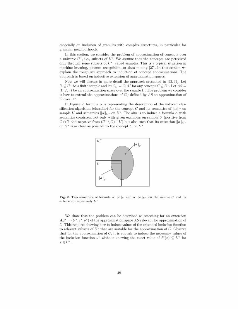
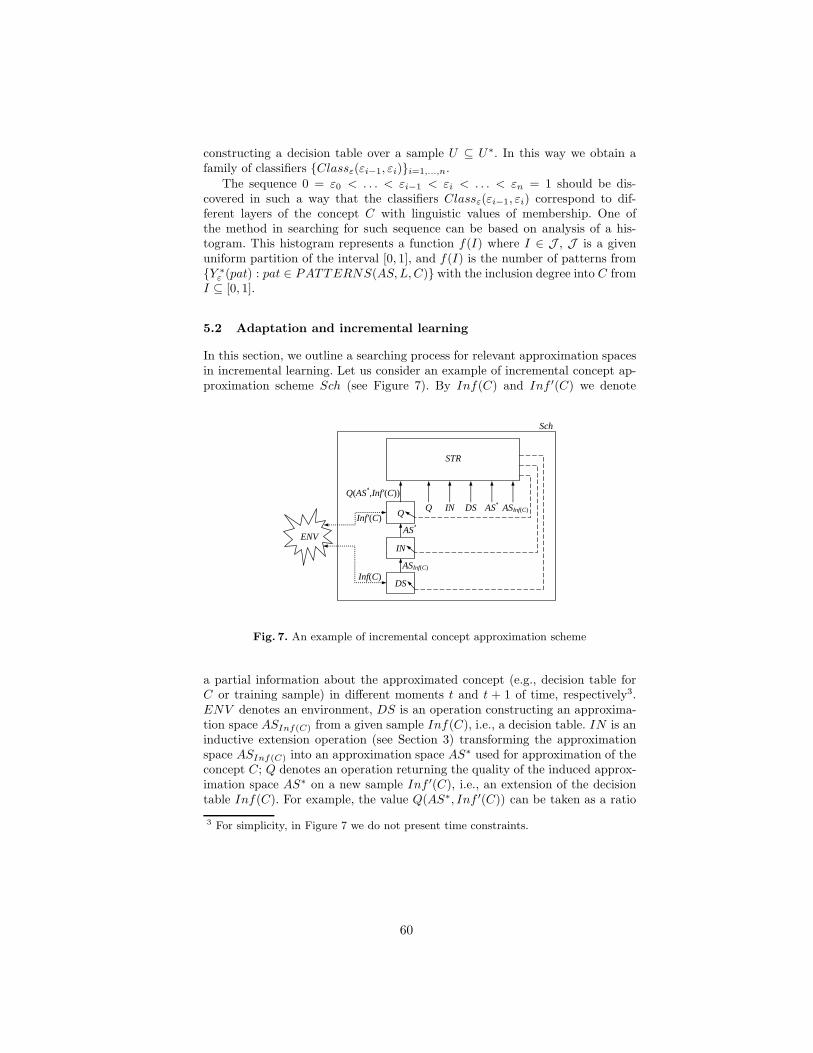
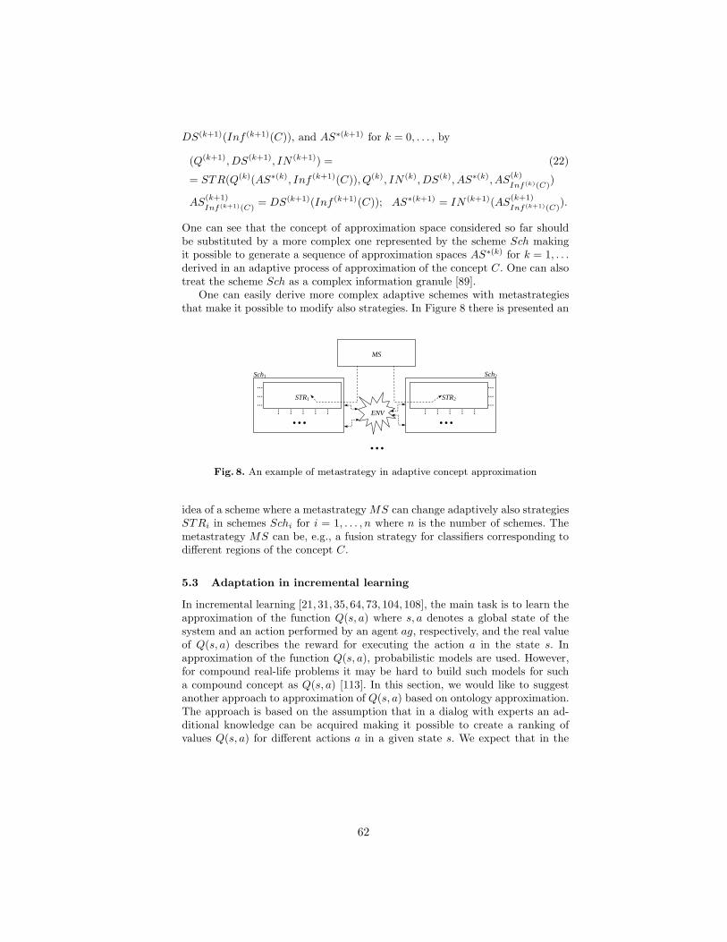
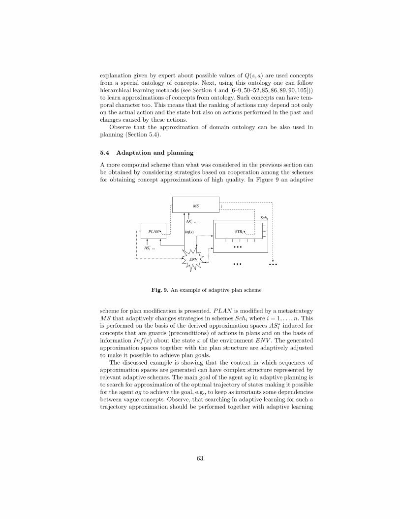
Rough Sets and Vague Concepts
Jan Bazan, Andrzej Skowron, Jaros law Stepaniukand Roman Swiniarski
Abstract. In this paper, we summarize and extend our previous resultson relationships between rough sets and vague concepts (see, e.g., [87, 5,104, 63, 92]). In particular, we consider imperfect specifications of vagueconcepts (e.g., by examples) and changes of knowledge about vague con-cepts. In these cases, the rough set based methods are allowing us toinduce temporary approximations of vague concepts. These approxima-tions may change with changes of knowledge about the approximatedconcepts. Approximation spaces used for concept approximation havebeen initially defined on samples of objects (decision tables) representingpartial information about concepts. Such approximation spaces definedon samples are next inductively extended on the whole object universe.This makes it possible to define the concept approximation on extensionsof samples. We discuss the role of inductive extensions of approximationspaces in searching for concept approximation. However, searching forrelevant inductive extensions of approximation spaces defined on samplesis infeasible for compound concepts. We outline an approach making thissearching feasible by using a concept ontology specified by domain knowl-edge and its approximation. We also extend this approach to a frameworkfor adaptive approximation of vague concepts by agents interacting withenvironments. This paper realizes a step toward approximate reasoningin multiagent systems (MAS), intelligent systems, and complex dynamicsystems (CAS).
1 Introduction
In this paper we discuss the rough set approach to vague concept approximation.There is a long debate in philosophy on vague concepts [36]. Nowadays, com-
puter scientists are also interested in vague (imprecise) concepts, e.g, many in-telligent systems should satisfy some constraints specified by vague concepts.Hence, the problem of vague concept approximation as well as preserving vaguedependencies especially in dynamically changing environments is important forsuch systems. Lotfi Zadeh [117] introduced a very successful approach to vague-ness. In this approach, sets are defined by partial membership in contrast to crispmembership used in the classical definition of a set. Rough set theory [59] ex-presses vagueness not by means of membership but by employing the boundaryregion of a set. If the boundary region of a set is empty it means that a particularset is crisp, otherwise the set is rough (inexact). The non-empty boundary re-gion of the set means that our knowledge about the set is not sufficient to definethe set precisely. In this paper some consequences on understanding of vagueconcepts caused by inductive extensions of approximation spaces and adaptive
38
concept learning are presented. A discussion on vagueness in the context of fuzzysets and rough sets can be found in [74].
Initially, the approximation spaces were introduced for decision tables (sam-ples of objects). The assumption was made that the partial information aboutobjects is given by values of attributes and on the basis of such informationabout objects the approximations of subsets of objects form the universe re-stricted to sample have been defined [59]. Starting, at least, from the early90s, many researchers have been using the rough set approach for construct-ing classification algorithms (classifiers) defined over extensions of samples. Thisis based on the assumption that available information about concepts is partial.In recent years, there have been attempts based on approximation spaces andoperations on approximation spaces for developing an approach to approxima-tion of concepts over the extensions of samples (see, e.g., [89, 93, 94, 104]). In thispaper, we follow this approach and we show that the basic operations relatedto approximation of concepts on extension of samples are inductive extensionsof approximation spaces. For illustration of the approach we use approximationspaces defined in [88]. Among the basic components of approximation spacesare neighborhoods of objects defined by the available information about objectsand rough inclusion functions between sets of objects. Observe that searchingfor relevant (for approximation of concepts) extensions of approximation spacesrequires tuning many more parameters than in the case of approximation of con-cepts on samples. The important conclusion from our considerations is that theinductive extensions defining classification algorithms (classifiers) are defined byarguments “for” and “against” of concepts. Each argument is defined by a tu-ple consisting of a degree of inclusion of objects into a pattern and a degree ofinclusion of the pattern into the concepts. Patterns in the case of rule-based clas-sifiers can be interpreted as the left hand sides of decision rules. The argumentsare discovered from available data and can be treated as the basic informationgranules used in the concept approximation process. For any new object, it ispossible to check the satisfiability of arguments and select arguments satisfiedto a satisfactory degree. Such selected arguments are fused by conflict resolu-tion strategies for obtaining the classification decision. Searching for relevantapproximation spaces in the case of approximations over extensions of samplesrequires discovery of many parameters and patterns including selection of rele-vant attributes defining information about objects, discovery of relevant patternsfor approximated concepts, selection of measures (similarity or closeness) of ob-jects into discovered patters for concepts, structure and parameters of conflictresolution strategy. This causes that in the case of more compound conceptsthe searching process becomes infeasible (see, e.g., [14, 113]). We propose to useas hints in the searching for relevant approximation spaces for compound con-cepts an additional domain knowledge making it possible to approximate suchconcepts. This additional knowledge is represented by a concept ontology [7–9,50–52,85, 86, 89, 90, 105] including concepts expressed in natural language andsome dependencies between them. We assume that the ontology of concept has ahierarchical structure. Moreover, we assume that for each concept from ontology
39
there is given a labelled set of examples of objects. The labels show the mem-bership for objects relative to the approximated concepts. The aim is to discoverthe relevant conditional attributes for concepts on different levels of a hierarchy.Such attributes can be constructed using the so-called production rules, produc-tions, and approximate reasoning schemes (AR schemes, for short) discoveredfrom data (see, e.g. [7–9, 50–52,85, 86, 89, 90, 105])). The searching for relevantarguments “for” and “against” for more compound concepts can be simplifiedbecause the searching can be organized along the derivations over the ontologyusing the domain knowledge.
Notice, that the searching process for relevant approximation spaces is drivenby some selected quality measures. While in some learning problems such mea-sures can be selected in a relatively easy way and remain unchanged duringlearning in other learning processes they can be only approximated on the basisof a partial information about such measures, e.g., received as the result of in-teraction with the environment. This case concerns, e.g., adaptive learning. Wediscuss the process of searching for relevant approximation spaces in differenttasks of adaptive learning [2, 19, 29, 32, 46, 48, 42, 106]. In particular, we presentillustrative examples of adaptation of observation to the agent’s scheme, incre-mental learning, reinforcement learning, and adaptive planning. Our discussionis presented in the framework of multiagent systems (MAS). The main conclu-sion is that the approximation of concepts in adaptive learning requires muchmore advanced methods, which, in particular, will make it possible to approxi-mate the quality measures together with approximation of concepts. We suggestthat this approach can be also based on approximation of ontology. In adap-tive learning, the approximation of concepts is constructed gradually and thetemporary approximations are changing dynamically in the learning process inwhich we are trying to achieve the approximation of the relevant quality. This, inparticular, causes, e.g., boundary conditions to change dynamically during thelearning process in which we are attempting to find the relevant approximationof the boundary regions of approximated vague concepts. This is consistent withthe requirement of the higher order vagueness [36] stating that the borderlinecases of vague concepts are not crisp sets. In Conclusions we point out someconsequences of this fact for further research on the rough set logic.
This paper is an extension and continuation of several papers (see, e.g., [7–9, 50–52, 87, 85, 86, 89, 90, 93, 104, 5, 96, 92]) on approximation spaces and vagueconcept approximation processes. In particular, we discuss here a problem ofadaptive learning of concept approximation. In this case, we are also searchingfor relevant approximation of the quality approximation measure. In a givenstep of the learning process, we have only a partial information about such ameasure. On the basis of such information we construct its approximation andwe use it for inducing approximation spaces relevant for concept approximation.However, in the next stages of the learning process, it may happen that afterreceiving new information form the environment, it is necessary to reconstructthe approximation of the quality measure and in this way we obtain a new
40
“driving force” in searching for relevant approximation spaces during the learningprocess.
This paper is organized as follows. Section 2 presents an introductory dis-cussion on sets and vagueness. In Section 3, we discuss inductive extensions ofapproximation spaces. We emphasize the role of discovery of special patternsand the so called arguments in inductive extensions. In Section 4, the role ofapproximation spaces in hierarchical learning is presented. Section 4, outlinesand approach based on approximation spaces during adaptive learning. In Sec-tion 6 (Conclusions), we summarize the discussion presented in the paper andwe present some further research directions based on approximation spaces toapproximate reasoning in multiagent systems and complex adaptive systems.
2 Sets and Vague Concepts
In this section, we put forward some general remarks on the concept of a set andthe place of rough sets in set theory.
The concept of a set is fundamental for the whole of mathematics. Modernset theory was formulated by George Cantor [16]. Bertrand Russell discoveredthat the intuitive notion of a set proposed by Cantor leads to antinomies [79].Two kinds of remedy for this problem have been proposed: axiomatization ofCantorian set theory and alternative set theories.
Another issue discussed in connection with the notion of a set or a concept isvagueness (see, e.g., [11, 24, 36, 37, 77, 80]). Mathematics requires that all math-ematical notions (including set) must be exact (Gottlob Frege [26]). However,philosophers (see, e.g., [36, 37, 74, 77]) and recently computer scientists (see, e.g.,[59, 117]) have become interested in vague concepts.
2.1 Sets
The notion of a set is one of, if not the most, basic concepts in mathematics. Allmathematical structures refer to it.
The definition of this notion and the creation of set theory are due to Ger-man mathematician Georg Cantor (1845-1918) [16], who laid the foundations ofcontemporary set theory over 100 years ago.
The birth of set theory can be traced back to his proof in 1873 of the un-countability of real line (i.e., the set of all real numbers is not countable) [15]. Itwas Bernhard Bolzano (1781-1848) who coined the term Menge (“set”), whichCantor used to refer to objects in his theory. According to Cantor, a set is acollection of any objects, which can be considered as a whole according to somelaw. As one can see, the notion of set is very intuitive and simple.
Mathematical objects such as relations, functions, numbers, are examples ofsets. In fact, set theory is needed in mathematics to provide rigor.
The notion of a set is not only fundamental for the whole of mathematics butit also plays an important role in natural language. We often speak about sets
41
(collections) of various objects of interest such as collection of books, paintingsand people.
The intuitive meaning of a set according to some dictionaries is the following:“A number of things of the same kind that belong or are used together.”
Webster’s Dictionary
“Number of things of the same kind, that belong together because they aresimilar or complementary to each other.”
The Oxford English Dictionary
Thus a set is a collection of things which are somehow related to each other butthe nature of this relationship is not specified in these definitions.
In fact, these definitions are due to the original definition given by Cantor.
2.2 Antinomies
In 1903, the renowned English philosopher Bertrand Russell (1872-1970) ob-served [79] that the intuitive notion of a set given by Cantor leads to logicalantinomies (contradictions), i.e., Cantor set theory is contradictory (there areother kinds of antinomies, which are outside the scope of this paper). A logicalantinomy (for simplicity, we refer to “antinomy” in the rest of this paper) ariseswhenever correct logical reasoning leads to a contradiction, i.e., to propositionsA and non-A, which is not allowed in logic.
As an example let us discuss briefly the so-called Russell’s antinomy. Considerthe set X containing all the sets Y , which are not the elements of themselves. Ifwe assume that X is its own element then X , by definition, cannot be its ownelement; while if we assume that X is not its own element then, according to thedefinition of the set X , it must be its own element. Thus while applying eachassumption we obtain contradiction.
Antinomies show that a set cannot be a collection of arbitrary elements, aswas stipulated by Cantor.
One could think that antinomies are ingenuous logical play, but it is not so.They question the essence of logical reasoning. That is why there have been at-tempts to “repair” Cantor’s theory for over 100 years or to substitute another settheory for it but the results so far are still not satisfactory. So, is all mathematicsbased on doubtful foundations?
As a remedy for this defect several axiomatizations of set theory have beenproposed (e.g., Zermelo and Fraenkel, 1904 [33]).
Instead of improvements of Cantors’ set theory by its axiomatization, somemathematicians proposed escape from classical set theory by creating a com-pletely new idea of a set, which would free the theory from antinomies [41, 114,1].
No doubt the most interesting proposal was given by Polish logician Stanis lawLesniewski, who introduced the relation of “being a part” instead of the mem-bership relation between elements and sets employed in classical set theory. In
42
his set theory called mereology, being a part is a fundamental relation [41]. Mere-ology is a significant part of recent studies on the foundations of mathematics(see, e.g., [12, 17, 25, 112, 39, 82]), artificial intelligence [98], cognitive science [97],natural language [23], and research in rough set theory (see, e.g., [70, 71, 67]).
The problem of finding an alternative to classical set theory has failed to besolved until now.
The deficiency of sets, mentioned above, has rather philosophical than prac-tical meaning, since sets used practically in mathematics are free from the abovediscussed faults. Antinomies are associated with very “peculiar” sets constructedin logic but not found in sets used in “everyday” mathematics. That is why wecan use mathematics safely.
2.3 Vagueness
Another issue discussed in connection with the notion of a set is vagueness.Mathematics requires that all mathematical notions (including set) must be ex-act, otherwise precise reasoning would be impossible. However, philosophers [36,37, 74, 78] and recently computer scientists (see, e.g., [3, 53, 54, 45, 18, 61, 62, 87,5, 22, 63, 101, 13, 69, 96, 92]) as well as other researchers have become interestedin vague (imprecise) concepts.
In classical set theory a set is uniquely determined by its elements. In otherwords, this means that every element must be uniquely classified as belongingto the set or not. That is to say the notion of a set is a crisp (precise) one. Forexample, the set of odd numbers is crisp because every number is either odd oreven.
In contrast to odd numbers, the notion of a beautiful painting is vague,because we are unable to classify uniquely all paintings into two classes: beautifuland not beautiful. Some paintings cannot be decided whether they are beautifulor not and thus they remain in the doubtful area. Thus, beauty is not a precisebut a vague concept.
Almost all concepts in natural language are vague. Therefore, common sensereasoning based on natural language must be based on vague concepts and noton classical logic. Interesting discussion of this issue can be found in [74].
The idea of vagueness can be traced back to the ancient Greek philosopherEubulides of Megara (ca. 400BC) who first formulated so called “sorites” (heap)and “falakros” (bald man) paradoxes (see, e.g., [36, 37]). The bald man paradoxgoes as follows: suppose a man has 100,000 hairs on his head. Removing one hairfrom his head surely cannot make him bald. Repeating this step we arrive atthe conclusion the a man without any hair is not bald. Similar reasoning can beapplied to a hip of stones.
Vagueness is usually associated with the boundary region approach (i.e.,existence of objects which cannot be uniquely classified relative to a set or itscomplement) which was first formulated in 1893 by the father of modern logic,German logician, Gottlob Frege (1848-1925) (see [26]).
According to Frege the concept must have a sharp boundary. To the conceptwithout a sharp boundary there would correspond an area that would not have
43
any sharp boundary–line all around. It means that mathematics must use crisp,not vague concepts, otherwise it would be impossible to reason precisely.
Summing up, vagueness is
– not allowed in mathematics;– interesting for philosophy;– nettlesome problem for natural language, cognitive science, artificial intelli-
gence, machine learning, and computer science.
Discussion on vague (imprecise) concepts includes the following issues [36]:
1. The presence of borderline cases.2. Boundary regions of vague concepts are not crisp.3. Vague concepts are susceptible to sorites paradoxes.
The existence of boundary cases are represented in rough sets by boundaryregions which are defined as crisp sets. However, boundary regions are definedrelative to a given set of attributes and in a more general setting to approx-imation space used for approximation. Hence, one can obtain many differentapproximations of vague concepts with many boundary regions. Note that theseare not all possible boundary regions. Next, many different methods for aggregat-ing the boundary regions can be used. In selection of these aggregating methodsagain some subjective or inductive assumptions are used. In the consequence,due to imperfect knowledge about the approximated concept, there is no possi-bility to define using classical set theory the absolute boundary region consistingall borderline cases for a given concept. In applications, the approximation ofvague concepts is induced using some optimization criteria, e.g., based on theminimum length principle. The obtained boundary region can be treated as atemporary approximation of the absolute boundary region. This view may bechanged, if our knowledge about the approximated concept was changed. Forexample, it is usually assumed that the understanding (approximation) of vagueconcepts (their semantics is determined by the satisfiability relation) dependson the agent’s knowledge, which is often changing. Hence, the approximation ofvague concepts by an agent should also be considered changing with time (thisis known as the concept drift). This problem is discussed in more detail in thispaper.
One can use rough sets for explanations of the existence of borderline in-stances discussed in the literature (see, e.g., [110, 18]). If x is and object andC is a concept than using the rough set approach the following situations mayhappen:
1. x is either C or not C but it is not known which case is true. This situationmay happen if in the decision table there is an object with unknown decisionassigned by, e.g., domain expert. Note that any further conditional attributescan not change this situation.
2. x is actually neither C nor non− P . This may happen if one considers onlycertain knowledge about C and then in may happen that the union of the
44
lower approximation of C and the lower approximation of the complementof C is not equal to the whole universe of objects. This situation may bealso happen for induced classifiers. For example, in the case of rule basedclassifiers, weights of rules matched by x which are voting for C and againstC may be not discernible to a satisfactory degree [50].
3. x is partially C, and partially non− C. By introducing the rough member-ship function one can obtain membership degrees different from 0 and 1 forobjects in the boundary region.
4. Depending on the context (perspective), x is sometimes C, and sometimesnon−C. This situation may happen when we deal with inconsistent decisiontables [63]. Following some context, sometimes one can add some new (con-ditional) attributes and with these new attributes the decision table becomesconsistent.
3 Approximation Spaces and their Inductive Extensions
In [59], any approximation space is defined as a pair (U, R), where U is a universeof objects and R ⊆ U × U is an indiscernibility relation defined by an attributeset.
The lower approximation, the upper approximation and the boundary regionare defined as crisp sets. It means that the higher order vagueness condition isnot satisfied [36]. We will return to this issue in Section 5.
We use the definition of approximation space introduced in [88]. Any approx-imation space is a tuple AS = (U, I, ν), where U is the universe of objects, Iis an uncertainty function, and ν is a measure of inclusion called the inclusionfunction, generalized in rough mereology to the rough inclusion [88, 94].
3.1 Uncertainty Function
In [91], the uncertainty function I defines for every object x from a given sampleU of objects, a set of objects with descriptions similar to x. The set I(x) is calledthe neighborhood of x. In our next papers (see, e.g. [95, 4, 92]) more generaluncertainty functions are considered for structural objects. The structures ofobjects are induced in hierarchical modeling. Let us recall some basic concepts.
LetPω(U∗) =
⋃
i≥1
P i(U∗),
where P 1(U∗) = P (U∗) and P i+1(U∗) = P (P i(U∗))) for i ≥ 1. For example, ifcard(U∗) = 2 and U∗ = x1, x2, then we obtain P 1(U∗) = ∅, x1, x2, x1,x2, P 2(U∗) = ∅, ∅, x1, x2, x1, x2, ∅, x1, ∅, x2, ∅, x1,x2, . . ., . . . . If card(U∗) = n, where n is a positive natural number, thencard(P 1(U∗)) = 2n and card(Pn+1(U∗)) = 2card(P n(U∗)), for n ≥ 1. For exam-ple, card(P 3(U∗)) = 222n
. Hence, we see that the levels of the powerset hierarchyare very rich and full automatic searching for relevant sets (structures) on such
45
levels is not feasible. However, this approach allows us to present in a uniformway foundations for modeling of granular computing aimed at inducing com-pound granules from different levels of the powerset hierarchy relevant for solv-ing the target task, e.g., approximation of complex concepts. For applications,it is necessary to restrict searching for relevant granules in relevant fragments ofthe powerset hierarchy. These fragments are defined by some sets of formulas.Discovery of such sets often is the big challenge for many problems.
Now, we consider uncertainty functions of the form I : U∗ −→ Pω(U∗). Thevalues of uncertainty functions are called granular neighborhoods. These gran-ular neighborhoods are defined by the so called granular formulas. The valuesof such uncertainty functions are not necessarily from P (U∗) but from Pω(U∗).Figure 1 presents an illustrative example of the uncertainty function with valuesin P 2(U∗) rather than in P (U∗). The generalization of neighborhoods discussedhere are also motivated by the necessity of modeling or discovery of complexstructural objects in solving problems of pattern recognition, machine learning,or data mining. These structural objects (granules) can be defined as sets onhigher levels of the powerset hierarchy. Among examples of such granules areindiscernibility or similarity classes of patterns or relational structures discov-ered in images, clusters of time widows, indiscernibility or similarity classes ofsequences of time windows representing processes, behavioral graphs (for moredetails see, e.g., [95, 4]).
*21U
ca =∧=
X U*
U
*201U
cba =∧=∧=
*01U
ba =∧=
x
Fig. 1. Uncertainty function I : U∗ → P 2(U∗). The neighborhood of x ∈ U∗ \ U ,where InfA(x) = (a, 1), (b, 0), (c, 2), does not contain training cases from U . Thegeneralizations of this neighborhood described by formulas ‖a = 1 ∧ c = 2‖U∗ and‖a = 1 ∧ b = 0‖U∗ have non empty intersections with U .
If X ∈ Pω(U∗) and U ⊆ U∗, then by X U we denote the set definedas follows (i) if X ∈ P (U∗) then X U = X ∩ U and (ii) for any i ≥ 1 ifX ∈ P i+1(U∗) then X U = Y U : Y ∈ X. For example, if U = x1,
46
U∗ = x1, x2 and X = x2, x1, x2 (X ∈ P 2(U∗)), then X U = Y U :Y ∈ X = Y ∩ U : Y ∈ X = ∅, x1.
In the above example, we discussed uncertainty functions assigning granulesfrom P 2(U∗) to objects from U∗ . We assume that objects from U and U∗ are ofatomic type with the type defined by attributes from a given information systemIS = (U, A) over U . For example, the type of objects from U may be identifiedwith ×a∈AVa. In a number of papers (see, e.g., [92]), we present methods ofdefining information systems with objects of higher order type (structural ob-jects). Such objects can be from different levels of Pω(U∗), i.e., they can belongto P k(U∗), for k > 2. Note that neighborhoods (e.g., indiscernibility classes)over such objects are sets of objects of higher order type from Pω(U∗).
3.2 Rough Inclusion Function
The second component of any approximation space is the rough inclusion func-tion [91].
One can consider general constraints which the rough inclusion functionsshould satisfy. In this section, we present only some examples of rough inclusionfunctions.
The rough inclusion function ν : P (U)×P (U) → [0, 1] defines the degree ofinclusion of X in Y , where X, Y ⊆ U and U is a finite sample of objects.
In the simplest case the standard rough inclusion function νSRI can be definedby (see, e.g., [91], [63]):
νSRI (X, Y ) =
card(X∩Y )
card(X) , if X 6= ∅1, if X = ∅. (1)
Some illustrative examples are given in Table 1.
Table 1. Illustration of Standard Rough Inclusion Function
X Y νSRI (X, Y )
x1, x3, x7, x8 x2, x4, x5, x6, x9 0
x1, x3, x7, x8 x1, x2, x4, x5, x6, x9 0.25
x1, x3, x7, x8 x1, x2, x3, x7, x8 1
It is important to note that an inclusion measure expressed in terms of theconfidence measure, widely used in data mining, was considered by Lukasiewicz[43] a long time ago in studies on assigning fractional truth values to logicalformulas.
For a definition of the inclusion function for more general granules, e.g.,partitions of objects, one can use a measure based on positive region [63], entropy[27] or rough entropy [56, 44]. Inclusion measures for more general granules werealso investigated [84, 10]. However, more work in this direction should be done,
47
especially on inclusion of granules with complex structures, in particular forgranular neighborhoods.
In this section, we consider the problem of approximation of concepts overa universe U∗, i.e., subsets of U∗. We assume that the concepts are perceivedonly through some subsets of U∗, called samples. This is a typical situation inmachine learning, pattern recognition, or data mining [27]. In this section weexplain the rough set approach to induction of concept approximations. Theapproach is based on inductive extension of approximation spaces.
Now we will discuss in more detail the approach presented in [93, 94]. LetU ⊆ U∗ be a finite sample and let CU = C∩U for any concept C ⊆ U∗. Let AS =(U, I, ν) be an approximation space over the sample U . The problem we consideris how to extend the approximations of CU defined by AS to approximation ofC over U∗.
In Figure 2, formula α is representing the description of the induced clas-sification algorithm (classifier) for the concept C and its semantics of ‖α‖U onsample U and semantics ‖α‖U∗ on U∗. The aim is to induce a formula α withsemantics consistent not only with given examples on sample U (positive fromC ∩ U and negative from (U∗ \ C) ∩ U) but also such that its extension ‖α‖U∗
on U∗ is as close as possible to the concept C on U∗ .
*Uα
Uα
*U
U
*Uα
Uα
*U
U
Fig. 2. Two semantics of formula α: ‖α‖U and α: ‖α‖U∗ on the sample U and itsextension, respectively U∗
We show that the problem can be described as searching for an extensionAS∗ = (U∗, I∗, ν∗) of the approximation space AS relevant for approximation ofC. This requires showing how to induce values of the extended inclusion functionto relevant subsets of U∗ that are suitable for the approximation of C. Observethat for the approximation of C, it is enough to induce the necessary values ofthe inclusion function ν∗ without knowing the exact value of I∗(x) ⊆ U∗ forx ∈ U∗.
48
We consider an example for rule-based classifiers1. However, the analogousconsiderations for k-NN classifiers, feed-forward neural networks, and hierarchi-cal classifiers [27] show that their construction is based on the inductive inclusionextension [87, 94].
Usually, neighborhoods of objects in approximation spaces are defined bysome formulas called patterns. Let us consider an example. Let AS∗ be a givenapproximation space over U∗ and let us consider a language L of patterns, wherex denotes an object from U∗. In the case of rule-based classifiers, patterns aredefined by feature value vectors. More precisely, in this case any pattern pat(x)is defined by a formula
∧(a, a(x)) : a ∈ A and va ∈ Va, where A is a givenset of condition attributes [59]. An object u ∈ U∗ is satisfying
∧(a, a(x)) : a ∈A and v ∈ Va if a(u) = a(x) for any a ∈ A, i.e., if and only if x, u are A-indiscernible [59]. The set of objects satisfying pat(x) in U∗, i.e., the semanticsof pat(x) in U∗, is denoted by ‖pat(x)‖U∗ . Hence, ‖pat(x)‖U∗ = [x]A where[x]A is the A-indiscernibility class of x ∈ U∗ [59]. By ‖pat(x)‖U we denote therestriction of ‖pat(x)‖ to U ⊆ U∗, i.e., the set ‖pat(x)‖ ∩ U . In the consideredcase, we assume that any neighborhood I(x) ⊆ U in AS is is expressible by apattern pat(x). It means that I(x) = ‖pat(x)‖U ⊆ U , where ‖pat(x)‖U denotesthe meaning of pat(x) restricted to the sample U .
We assume that for any object x ∈ U∗, only partial information about xresulting, e.g., from a sensor measurement represented by a pattern pat(x) ∈L with semantics ‖pat(x)‖U∗ ⊆ U∗ defining the neighborhood of x in U∗ isavailable. Moreover, only partial information such as ‖pat(x)‖U is available aboutthis set. In particular, relationships between information granules over U∗, e.g.,‖pat(x)‖U∗ and ‖pat(y)‖U∗ , for different x, y ∈ U∗, are known only to a degreeestimated by using relationships between the restrictions of these sets to thesample U , i.e., between sets ‖pat(x)‖U∗ ∩ U and ‖pat(y)‖U∗ ∩ U .
The set pat(x) : x ∈ U of patterns (defined by the whole set of attributesA from an approximation space AS) is usually not relevant for approximation ofthe concept C ⊆ U∗. Such patterns can be too specific or not general enough, andcan directly be applied only to a very limited number of new sample elements.For example, if for a new object x ∈ U∗ \ U the set ‖pat(x)‖U can be disjointwith all sets ‖pat(y)‖U for y ∈ U .
However, by using some generalization strategies, one can induce from pat-terns belonging to pat(x) : x ∈ U some new patterns that are relevant forapproximation of concepts over U∗.
Usually, first we define a new set PAT of patterns, which are candidatesfor relevant approximation of a given concept C. A typical example of the set ofsuch patterns used in the case of rule based classifiers can be defined by droppingsome descriptors from patterns constructed over the whole set of attributes, i.e.,∧(a, a(x)) : a ∈ B and va ∈ Va : B ⊆ A and x ∈ U. Among such patternswe search for the left hand sides of decision rules.
1 For simplicity of reasoning we consider only binary classifiers, i.e. classifiers with twodecision classes. One can easily extend the approach to the case of classifiers withmore decision classes.
49
The set PATTERNS(AS, L, C) can be selected from PAT using some qual-ity measures evaluated on meanings (semantics) of patterns from this set re-stricted to the sample U . Often such measures are based on the numbers ofexamples from the concept CU and its complement that support (satisfy) agiven pattern. For example, if the confidence coefficient
card(‖pat‖U ∩ CU )card(‖pat(x)‖U )
, (2)
where pat ∈ PAT , is at least equal to a given threshold and the support
card(‖pat‖U ∩ CU )card(U
, (3)
is also at least equal to a given threshold than we select pat as a member ofPATTERNS(AS, L, C).
Next, on the basis of some properties of sets definable by patterns fromPATTERNS(AS, L, C) over U , we induce approximate values of the inclusionfunction ν∗(X, C) on subsets of X ⊆ U∗ definable by any such pattern and theconcept C. For example, we assume that the value of the confidence coefficientis not changing significantly if we move from U to U∗, i.e.,
card(‖pat‖U ∩CU )card(‖pat(x)‖U )
≈ card(‖pat‖U∗ ∩ C)card(‖pat(x)‖U∗)
, (4)
Next, we induce the value of ν∗ on pairs (X, Y ) where X ⊆ U∗ is defin-able by a pattern from pat(x) : x ∈ U∗ and Y ⊆ U∗ is definable by a pat-tern from PATTERNS(AS, L, C). For example, if pat(x) =
∧(a, a(x)) : a ∈A and va ∈ Va and pat is obtained from pat(x) by dropping some conjuncts thenν∗(‖pat(x)‖U∗ , ‖pat‖)U∗) = 1 because ‖pat‖U∗ ⊆ ‖pat(x)‖U∗ . In a more generalcase, one can estimate the degree of inclusion of ‖pat(x)‖U∗ into ‖pat‖U∗ usingsome similarity degrees defined between formulas from PATTERNS(AS, L, C)and PAT . For example, one can assume that the values of attributes on x whichoccur in pat are not necessarily the same but similar. Certainly, such a similarityshould be also defined or learned from data.
Finally, for any object x ∈ U∗ \ U we induce the degree ν∗(‖pat(x)‖U∗ , C)applying a conflict resolution strategy Conflict res (e.g, a voting strategy) totwo families of tuples:
(ν∗(‖pat(x)‖U∗ , ‖pat‖U∗), pat, ν∗(‖pat‖U∗ , C)) : pat ∈ PATTERNS(AS, L, C).(5)
Let us observe that conflicts can occur due to inductive reasoning in estimationof values of ν∗. For some x ∈ U∗ and pat, pat′ ∈ PATTERNS(AS, L, C) thevalues ν∗(‖pat(x)‖U∗ , ‖pat‖U∗), ν∗(‖pat(x)‖U∗ , ‖pat′‖U∗) can be both large (i.e.,close to 1) and at the same time the value ν∗(‖pat‖U∗ , C) can be small (i.e., closeto 0) and the value of ν∗(‖pat′‖U∗ , C) can be large.
Values of the inclusion function for the remaining subsets of U∗ can be chosenin any way – they do not have any impact on the approximations of C. Moreover,
50
observe that for the approximation of C we do not need to know the exact valuesof uncertainty function I∗ – it is enough to induce the values of the inclusionfunction ν∗. The defined extension ν∗ of ν to some subsets of U∗ makes it possibleto define an approximation of the concept C in a new approximation space AS∗.
To reduce the number of conditions from (5) one can use the so called argu-ments “for” and “against” discussed, e.g., in [90].
Any C-argument, where C ⊆ U∗ is a concept is a triple
(ǫ, pat, ǫ′) (6)
where ǫ, ǫ′ ∈ [0, 1] are degrees and pat is a pattern from PATTERNS(AS, L, C).The argument arg = (ε, pat, ε′) is satisfied by a given object x ∈ U∗, in
symbols x |=C arg, if and only if the following conditions are satisfied:
ν∗(‖pat(x)‖U∗ , ‖pat‖U∗) ≥ ε; (7)ν∗(‖pat‖U∗ , C) ≥ ε′.
The idea of C-arguments is illustrated in Figure 3.
ε'ε
Cpat)(xpat
Fig. 3. C-argument
Instead of all conditions from (5) only some arguments “for” and “against”C are selected and the conflict resolution strategy is based on them. For anynew object the strategy resolves conflicts between selected arguments “for” and“against” C which are satisfied by the object.
The very simple strategy for selection of arguments is the following one.The C-argument arg = (ε, pat, ε′) is called the argument “for” C if ε ≥ t andε′ ≥ t′, where t, t′ > 0.5 are given thresholds. The argument arg is “against”C, if this argument is the argument for the complement of C, i.e., for U∗ \ C.However, in general this may be not relevant method and the relevant argumentsshould be selected on the basis of more advanced quality measures. They cantake into account , e.g., the support of patterns in arguments (see Section 5.1),their coverage, independence from other arguments, or relevance in searching forarguments used for approximation of more compound concepts in hierarchicallearning.
51
One can define the lower approximation and upper approximation of theconcept C ⊆ U∗ in the approximation space AS∗ by
LOW (AS∗, C) = x ∈ U∗ : ν∗(I∗(x), C) = 1, (8)UPP (AS∗, C) = x ∈ U∗ : ν∗(I∗(x), C) > 0.
From the definition we have:
LOW (AS∗, C) ∩ U ⊆ C ∩ U ⊆ UPP (AS∗, C) ∩ U. (9)
However, in general the following equalities do not hold:
LOW (AS, C ∩ U) = LOW (AS∗, C) ∩ U, (10)UPP (AS, C ∩ U) = UPP (AS∗, C) ∩ U.
One can check that in the case of standard rough inclusion [89] we have:
LOW (AS, C ∩ U) ⊇ LOW (AS∗, C) ∩ U, (11)UPP (AS, C ∩ U) ⊆ UPP (AS∗, C) ∩ U.
Following the minimal length principle [75, 76, 100] some parameters of the in-duced approximation spaces are tuned to obtain a proper balance between thedescription length of the classifier and its consistency degree. The consistencydegree on a given sample U of data can be represented by degrees to which thesets defined in equalities (10) are close. The description length is measured bydescription complexity of the classifier representation. Among parameters whichare tuned are attribute sets used in the classifier construction, degrees of inclu-sion of patterns defined by objects to the left hand sides of decision rules, degreesof inclusion of patterns representing the left hand sides of decision rules in thedecision classes, the specificity or support of these patterns, parameters of theconflict resolution strategy (e.g., set of arguments and parameters of arguments).
We can summarize our considerations in this section as follows. The induc-tive extensions of approximation spaces are basic operations on approximationspaces in searching for relevant approximation spaces for concept approxima-tion. The approximation of concepts over U∗ is based on searching for relevantapproximation spaces AS∗ in the set of approximation spaces defined by induc-tive extensions of a given approximation space AS. For any object x ∈ U∗ \ U ,the value ν∗(I∗(x), C) of the induced inclusion function ν∗ is defined by conflictresolution strategy from collected arguments for classifying x to C and fromcollected arguments against classifying x to C.
4 Approximation Spaces in Hierarchical Learning
The methodology for approximation spaces extension presented in Section 3 iswidely used for construction of rule based classifiers. However, this methodologycannot be directly used for concepts that are compound because of problems
52
with inducing of the relevant set PATTERNS(AS, L, C) of patterns. For suchcompound concepts, hierarchical learning methods have been developed (see,e.g., [6–9, 50–52,85, 86, 89, 90, 105]).
We assume that domain knowledge is available about concepts. There is givena hierarchy of concepts and dependencies between them creating the so-calledconcept ontology. Only partial information is available about concepts in thehierarchy. For concepts from the lowest level of hierarchy, decision tables withcondition attributes representing sensory measurements are given. Classifiers forthese concepts are induced (constructed) from such decision tables. Assumingthat classifiers have been induced for concepts from some level l of the hierarchy,we are aiming at inducing classifiers for concepts on the next l + 1 level of thehierarchy. It is assumed that for concepts on higher levels there are given samplesof objects with information about their membership values relative to the con-cepts. The relevant patterns for approximation of concepts from the l+1 level arediscovered using (i) these decision tables, (ii) information about dependencieslinking concepts from the level l + 1 with concepts from the level l, and (iii) pat-terns discovered for approximation of concepts from the level l of the hierarchy.Such patterns define condition attributes (e.g., by the characteristic functionsof patterns) in decision tables. Next, from such approximation of concepts areinduced. In this way, also, the neighborhoods for objects on the level l + 1 aredefined. Observe also that the structure of objects on the higher level l + 1 isdefined by means of their parts from the level l. In this section, for simplicity ofreasoning, we assume that on each level the same objects are considered. To thisend, we also assume that rough inclusion functions from approximation spacesare standard rough inclusion functions [89].
Now we outline a method of construction of patterns used for approxima-tion of concepts from a given level of concept hierarchy by patterns used forapproximation of concepts belonging to the lower level of the hierarchy. Thisapproach has been elaborated in a number of papers cited above, in particularin [90]. Assume that a concept C belongs to a level l + 1 of the hierarchy. Weoutline the idea of searching for sets PATTERNS(AS, L, C) of patterns for aconcept C, where AS is an approximation space discovered for approximation ofthe concept C and L is a language in which discovered patterns are expressed.
To illustrate this idea, let us consider and example of a dependency for aconcept C from domain knwoledge:
if C1 and C2 then C, (12)
where C1, C2, C are vague concepts. Analogously, let us consider a dependencyfor the complement of C:
if C′1 and C′
2 then ¬C. (13)
In general, we should consider a set with many dependencies with differentconcepts on the right hand sides of dependencies (creating, e.g., a partition ofthe universe) and in the process of generating arguments “for” and “against” aselected concept C are involved other vague dependencies from the given set. Let
53
us recall that such a set of concepts and dependencies between them is specifiedin a given domain knowledge.
To approximate the target concept C, relevant patterns for C and ¬C shouldbe derived. The main idea is presented in Figure 4 and Figure 5. We assume thatfor any considered concept and for each pattern selected for this concept a degreeof its inclusion into the concept can be estimated.
2ε1ε
1C1pat2C2pat
Cpat
ε
Fig. 4. An illustration of pattern construction
1ε2ε
1C1pat
'1ε
'2ε
2C2pat
ε'ε
Cpat
Fig. 5. An illustration of production rule
In Figure 4 it is shown that for patterns pat1, pat2 (e.g., left hand sides ofdecision rules in case of a rule based classifiers) for (or against) C1 and C2 and
54
their inclusion degrees ǫ1 and ǫ2 into C1 and C2, respectively, it is constructeda pattern pat for (or against) C together with estimation of its inclusion degreeǫ to the concept C.
Figure 5 represents a construction of the target argument (ǫ, pat, ǫ′) for Cfrom arguments (ǫ1, pat1, ǫ
′1) and (ǫ2, pat2, ǫ
′2) for C1 and C2, respectively. Such
a construction
if (ǫ1, pat1, ǫ′1) and (ǫ2, pat2, ǫ
′2) then (ǫ, pat, ǫ′) (14)
is called a production rule for the dependency (12). Such a production rule istrue at a given object x if and only if the following implication holds:
if x |=C1 (ǫ1, pat1, ǫ′1) and x |=C2 (ǫ2, pat2, ǫ
′2) then x |=C (ǫ, pat, ǫ′). (15)
Certainly, it is necessary to search for production rules of the high quality(with respect to some measures) making possible to construct “strong” argu-ments in the conclusion of the production from “strong” arguments in the pre-misses of the production rule. The quality of arguments is defined by means ofrelevant degrees of inclusion in these arguments and properties of patterns (suchas support or description length).
The quality of arguments for concepts from the level l + 1 can be estimatedon the basis properties of arguments for the concepts from the level l from whichthese arguments have been constructed. In this estimation are used decision ta-bles delivered by domain experts. Such decision tables consist of objects withdecision values equal to the membership degrees of objects relative to the con-cept or to its complement. In searching for productions of high quality, we useoperations called constrained sums (see, e.g., [99]). Using these operations thereare performed joins of information systems representing patterns appearing inarguments from the premise of production. The join is parameterized by con-straints helping by tuning these parameters to filter the relevant objects fromcomposition of patterns used for constructing a pattern for the concept C onthe level l + 1 for the argument in the conclusion of the production rule. More-over, the production rules may be composed into the so called approximationreasoning schemes (AR schemes, for short). This makes it possible to generatepatterns for approximation of concepts on the higher level of the hierarchy (see,e.g., [6–9, 50–52, 86, 90]). In this way one can induce gradually for any concept Cin the hierarchy a relevant set of arguments (based on the relevant set of patternsPATTERNS(AS, L, C) of patterns; see Section 4) for approximation of C.
We have recognized that for a given concept C ⊆ U∗ and any object x ∈ U∗,instead of crisp decision about the relationship of I∗(x) and C, we can gathersome arguments for and against it only. Next, it is necessary to induce from sucharguments the value ν∗(I(x), C) using some strategies making it possible to re-solve conflicts between those arguments [27, 89]. Usually some general principlesare used such as the minimal length principle [27] in searching for algorithmscomputing an extension ν∗(I(x), C). However, often the approximated conceptover U∗ \ U is too compound to be induced directly from ν(I(x), C). This isthe reason that the existing learning methods are not satisfactory for inducing
55
high quality concept approximations in case of complex concepts [113]. Therehave been several attempts trying to omit this drawback. In this section we havediscussed the approach based on hierarchical (layered) learning [105].
There are some other issues which should be discussed in approximation ofcompound vague concepts. Among them are issues related to adaptive learningand construction or reconstruction of approximation spaces in interaction withenvironments. In the following section, we consider an agent learning some con-cepts. This agent is learning the concepts in interaction with the environments.Different types of interaction are defining different types of adaptive learning pro-cesses. In particular one can distinguish incremental learning [30, 47, 109, 116],reinforcement learning [21, 31, 35, 64, 73, 108], competitive or cooperative learn-ing [32]. There are several issues, important for adaptive learning that shouldbe mentioned. For example, the compound target concept which we attempt tolearn can gradually change over time and this concept drift is a natural extensionfor incremental learning systems toward adaptive systems. In adaptive learningit is important not only what we learn but also how we learn, how we measurechanges in a distributed environment and induce from them adaptive changesof constructed concept approximations. The adaptive learning for autonomoussystems became a challenge for machine learning, robotics, complex systems,and multiagent systems. It is becoming also a very attractive research area forthe rough set approach. Some of these issues will be discussed in the followingsection.
5 Approximation Spaces in Adaptive Learning
There are different interpretations of the terms adaptive learning and adaptivesystems (see, e.g., [2, 19, 29, 32, 46, 48, 42, 106]). We mean by adaptive a systemthat learns to change with its environment. Our understanding is closest to thespirit of what appears in [19, 29]. In complex adaptive systems (CAS), agentsscan their environment and develop a schema for action. Such a schema definesinteractions with agents surrounding it together with information and resourcesflow externally [19]. In this section, we concentrate only on some aspects ofadaptive learning. The other issues of adaptive learning in MAS and CAS willbe discussed elsewhere.
In particular, we would like to discuss the role of approximation spaces inadaptive learning.
In this paper, we consider the following exemplary situation. There is anagent ag interacting with another agent called the environment (ENV). Interac-tions are represented by actions [28, 111] performed by agents. These actions arechanging values of some sensory attributes of agents. The agent ag is equippedwith ontology of vague concepts consisting of vague concepts and dependenciesbetween them.
There are three main tasks of the agent ag: (i) adaptation of observation tothe agent’s scheme, (ii) adaptive learning of the approximations of vague con-
56
cepts, and (iii) preserving constraints (e.g., expressed by dependencies betweenconcepts).
Through adaptation of observation to the agent’s scheme agent becomes morerobust and can handle more variability [19].
Approximation of vague concepts by the agent ag requires development ofsearching methods for relevant approximation spaces which create the basis forapproximation of concepts. Observe that the approximations of vague conceptsare dynamically changing in adaptive learning when new knowledge about ap-proximated concept is obtained by the agent ag. In particular, from this it followsthat the boundary regions of approximated concepts are dynamically changingin adaptive learning. For each approximated concept we obtain a sequence ofboundary regions rather than a single crisp boundary region. By generating thissequence we are attempting to approximate the set of borderline cases of a givenvague concept. Hence, if the concept approximation problem is considered inadaptive framework the higher order postulate for vague concepts is satisfied(i.e., the set of borderline cases of any vague concept can not be crisp) [36, 87,93].
The third task of the agent ag requires learning of a planning strategy. Thisis a strategy for predicting plans (i.e., sequences of actions) on the basis of ob-served changes in the satisfiability of the observed concepts from ontology. Byexecuting plans the actual state of the system is transformed to a state satisfy-ing the constraints. Changes in the environments can cause that the executedplans should be reconstructed dynamically by relevant adaptive strategies. Inour example actions performed by the agent ag are adjusting values of sensoryattributes which are controllable by ag.
Before we will discuss the mentioned above tasks in more detail we wouldlike to add some comments on interaction between agents.
The interactions among agents belong to the most important ingredients ofcomputations realized by multiagent systems [42]. In particular, adaptive learn-ing agents are interact, in particular, with their environments. In this section,we will continue our discussion on adaptive learning by agents interacting withenvironment. Some illustrative examples of interactions which have influence onthe learning process are presented.
Let us consider two agents ag and ENV representing the agent learningsome concepts and the environment, respectively. By ag s(t) and ENV s(t)we denote (information about) the state of agents ag and ENV at the timet, respectively. Such an information can be represented, e.g., by a vector ofattribute values Aag and AENV , respectively [94]. The agent ag is computingthe next state ags(t + 1) using his own transition relation −→ag applied to theresult of interaction of ags(t) and ENVs(t). The result of such an interaction wedenote by ags(t) ⊕ENV ENVs(t) where ⊕ENV is an operation of interaction ofENV on the state of ag. Hence, the following condition holds:
ags(t)⊕ENV ENVs(t) −→ag ags(t + 1). (16)
57
Analogously, we obtain the following transition for environment states:
ags(t)⊕ag ENVs(t) −→ENV ENVs(t + 1). (17)
In our examples, we will concentrate on two examples of interactions. Inthe first example related to incremental learning (see, e.g., [47, 109, 30, 116]),we assume that ags(t) ⊕ENV ENVs(t) is obtained by extending of ags(t) by anew information about some new sample of objects labelled by decisions. Thestructure of ags(t) is much more compound than in non-incremental learning.This will be discussed in one of the following section together with some aspectsof adaptation in incremental learning. These aspects are related to searchingfor relevant approximation spaces. In the discussed case, we also assume thatags(t) ⊕ag ENVs(t), i.e., there is no interaction of the agentag on the environ-ment. In our second example, the agent ag can change the state of ENV byperforming some actions or plans which change the state of the environment.
5.1 Adaptation of observation to the agent’s scheme
In this section, we present two illustrative examples of adaptation of observationto the agent’s scheme. In the consequence of such an adaptation, the agent’sscheme becomes more robust relative to observations.
In the first example, we consider instead of patterns pat(x) (see Section 3)mode general patterns which are obtained by granulation of such patterns usinga similarity relation τ . Assuming that the object description pat(x) is defined by∧(a, a(x)) : a ∈ A and va ∈ Va one can define such a similarity τ on descrip-tion of objects, e.g., by a composition of similarity relations on attribute valuesets (see, e.g., [40, 49, 88])2. Then instead of patterns pat(x) we obtain patternspatτ (x) with the semantics defined by ‖patτ (x)‖U∗ = y ∈ U∗ : pat(x)τpat(y).The definition of satisfiability of arguments (7) changes as follows
Observe, that ‖patτ (x)‖U∗ is usually supported by many more objects than‖pat(x)‖U∗ . Hence, if it is possible to tune the parameters of τ in such a way thatthe first condition in (18) is satisfied for sufficiently large ε than the obtainedargument is much more robust than the previous one, i.e., it is satisfied by muchmore objects than the previous one pat(x) and at the same time the requirementrelated to the degrees of inclusion is preserved.
Our second example concerns construction of more robust production rulesand productions (sets of production rules corresponding to the same dependencybetween vague concepts) (see Figure 6). Patterns in such productions representdifferent layers of vague concepts and are determined by the linguistic valuesof membership such as small, medium, high (see, e.g., [9]). These more generalpatterns are constructed using information granulation [94]. Let us consider a2 Note, that the similarity relation τ has usually many parameters which should be
tuned in searching for relevant similarity relations.
58
C4 ≥≥≥≥ ” large”
C3 ≥≥≥≥ ” large”
C5 ≥≥≥≥ ”large”
C4 ≥≥≥≥ ” medium”
C3 ≥≥≥≥ ” large”
C5 ≥≥≥≥ ” medium”
C4 ≥≥≥≥ ” small” C3 ≥≥≥≥ ” medium”
C5 ≥≥≥≥ ” small”
C2 ≥≥≥≥ ” large”
C1 ≥≥≥≥ ” medium”
C3 ≥≥≥≥ ”large”
C2 ≥≥≥≥ ” medium”
C1 ≥≥≥≥ ”small”
C3 ≥≥≥≥ ” medium”
C2 ≥≥≥≥ ” small”
C1 ≥≥≥≥ ” small”
C3 ≥≥≥≥ ” small”
C2 ≥≥≥≥ ” medium”
C1 ≥≥≥≥ ”small”
C4 ≥≥≥≥ ” small”
C5 ≥≥≥≥ ” small”
C4 ≥≥≥≥ ” small”
C3 ≥≥≥≥ ” medium”
C5 ≥≥≥≥ ” small”
C2 ≥≥≥≥ ” medium”
C1 ≥≥≥≥ ”small”
AR-scheme as a new
production rule
Production for C5
AR-scheme
Production for C3
Fig. 6. An illustration of production and AR scheme
simple example of information granulation. Observe that the definition of thesatisfiability of arguments given by (7) is not unique. One can consider thedecision table (U, A, d), where A is a given set of condition attributes [59] andthe decision d is the characteristic function of the set Yε(pat) = y ∈ U :ν(‖pat(y)‖U , ‖pat‖U)) ≥ ε. From this decision table can be induced the classifierClass(pat) for the concept Y ∗
ε (pat) = y ∈ U∗ : ν∗(‖pat(y)‖U∗ , ‖pat‖U∗)) ≥ ε.Any object x ∈ U∗ is satisfying the C-argument (6) if and only if the followingcondition is satisfied:
ν∗(Y ∗ε (pat), C) ≥ ε′. (19)
The satisfiability of (19) is estimated by checking if the following condition holdson the sample U :
ν(Yε(pat), C ∩ U) ≥ ε′. (20)
We select only the arguments (ε, pat, ε′) with the maximal ε′ satisfying (20) forgiven ε and pat.
Assume that 0 = ε0 < . . . < εi−1 < εi < . . . < εn = 1. For any i = 1, . . . , nwe granulate a family of sets
Y ∗ε (pat) : pat ∈ PATTERNS(AS, L, C) and ν∗(Y ∗
ε (pat), C) ∈ [εi−1, εi)(21)
into one set Y ∗ε (εi−1, εi). Each set Y ∗
ε (εi−1, εi) is defined by an induced classifierClassε(εi−1, εi). The classifiers are induced, in an analogous way as before, by
59
constructing a decision table over a sample U ⊆ U∗. In this way we obtain afamily of classifiers Classε(εi−1, εi)i=1,...,n.
The sequence 0 = ε0 < . . . < εi−1 < εi < . . . < εn = 1 should be dis-covered in such a way that the classifiers Classε(εi−1, εi) correspond to dif-ferent layers of the concept C with linguistic values of membership. One ofthe method in searching for such sequence can be based on analysis of a his-togram. This histogram represents a function f(I) where I ∈ J , J is a givenuniform partition of the interval [0, 1], and f(I) is the number of patterns fromY ∗
ε (pat) : pat ∈ PATTERNS(AS, L, C) with the inclusion degree into C fromI ⊆ [0, 1].
5.2 Adaptation and incremental learning
In this section, we outline a searching process for relevant approximation spacesin incremental learning. Let us consider an example of incremental concept ap-proximation scheme Sch (see Figure 7). By Inf(C) and Inf ′(C) we denote
STR
Q
IN
DS
ENV
Inf(C)
Inf'(C)
ASInf(C)
AS*
Q(AS*,Inf'(C))
ASInf(C) AS* DS IN Q
Sch
Fig. 7. An example of incremental concept approximation scheme
a partial information about the approximated concept (e.g., decision table forC or training sample) in different moments t and t + 1 of time, respectively3.ENV denotes an environment, DS is an operation constructing an approxima-tion space ASInf(C) from a given sample Inf(C), i.e., a decision table. IN is aninductive extension operation (see Section 3) transforming the approximationspace ASInf(C) into an approximation space AS∗ used for approximation of theconcept C; Q denotes an operation returning the quality of the induced approx-imation space AS∗ on a new sample Inf ′(C), i.e., an extension of the decisiontable Inf(C). For example, the value Q(AS∗, Inf ′(C)) can be taken as a ratio
3 For simplicity, in Figure 7 we do not present time constraints.
60
of the number of objects from Inf ′(C) that are classified correctly (relative tothe decision values from Inf ′(C)) by the classification algorithm (classifier) forC defined by AS∗ (see Section 3) to the number of all objects in Inf ′(C).
The double-ended arrows leading into and out of ENV illustrate an inter-action between agent ag and the environment ENV . In the case of a simpleincremental learning strategy only samples of C are communicated by ENVto ag. More compound interactions between ag and ENV will be discuss later.They can be related to reaction from ENV on predicted by ag decisions (actions,plans) (see, e.g., award and penalty policies in reinforcement strategies [21, 31,35, 64, 73, 108]).
STR is a strategy that adaptively changes the approximation of C by mod-ifying the quality measure Q, the operation of inductive extension IN , and theoperation DS of constructing the approximation space ASInf(C) from the sam-ple Inf(C). Dotted lines outgoing from the box labelled by STR in Figure 7are illustrating that the strategy STR after receiving the actual values of inputits parameters is changing them (e.g., in the next moment of time). To makeFigure 7 more readable the dotted lines are pointing to only one occurrence ofeach parameter of STR but we assume that its occurrences on the input forSTR are modified too.
In the simple incremental learning strategy, the quality measure is fixed.The aim of the strategy STR is to optimize the value of Q in the learningprocess. This means that in the learning process we would like to reach as soon aspossible an approximation space which will guarantee the quality of classificationmeasured by Q to be almost optimal. Still, we do not know how to controlby STR this optimization. For example, should this strategy be more like theannealing strategy [38], then it is possible to perform more random choices atthe beginning of the learning process and next be more “frozen” to guarantee thehigh convergence speed of the learning process to (semi-)optimal approximationspace. In the case of more compound interactions between ag and ENV , e.g.,in reinforcement learning, the quality measure Q should be learned using, e.g.,awards or penalties received as the results of such interactions. This means thattogether with searching for an approximation space for the concept it is necessaryto search for an approximation space over which the relevant quality measurecan be approximated with high quality.
The scheme Sch describes an adaptive strategy ST modifying the inducedapproximation space AS∗ with respect to the changing information about theconcept C. To explain this in more detail, let us first assume that a proce-dure newC(ENV, u) is given returning from the environment ENV and cur-rent information u about the concept C a new piece of information about thisconcept (e.g., an extension of a sample u of C). In particular, Inf (0)(C) =newC(ENV, ∅) and Inf (k+1)(C) = newC(ENV, Inf (k)(C)) for k = 0, . . .. InFigure 7 Inf ′(C) = Inf (1)(C). Next, assuming that operations Q(0) = Q,DS(0) = DS, IN (0) = IN are given, we define Q(k+1), DS(k+1), IN (k+1),
61
DS(k+1)(Inf (k+1)(C)), and AS∗(k+1) for k = 0, . . . , by
(Q(k+1), DS(k+1), IN (k+1)) = (22)
= STR(Q(k)(AS∗(k), Inf (k+1)(C)), Q(k), IN (k), DS(k), AS∗(k), AS(k)
Inf(k)(C))
AS(k+1)
Inf(k+1)(C)= DS(k+1)(Inf (k+1)(C)); AS∗(k+1) = IN (k+1)(AS
(k+1)
Inf(k+1)(C)).
One can see that the concept of approximation space considered so far shouldbe substituted by a more complex one represented by the scheme Sch makingit possible to generate a sequence of approximation spaces AS∗(k) for k = 1, . . .derived in an adaptive process of approximation of the concept C. One can alsotreat the scheme Sch as a complex information granule [89].
One can easily derive more complex adaptive schemes with metastrategiesthat make it possible to modify also strategies. In Figure 8 there is presented an
ENV
STR1
…
Sch1
…
…
… …
…
…
…
…
STR2
…
Sch2
…
…
… …
…
…
…
…
MS
…
Fig. 8. An example of metastrategy in adaptive concept approximation
idea of a scheme where a metastrategy MS can change adaptively also strategiesSTRi in schemes Schi for i = 1, . . . , n where n is the number of schemes. Themetastrategy MS can be, e.g., a fusion strategy for classifiers corresponding todifferent regions of the concept C.
5.3 Adaptation in incremental learning
In incremental learning [21, 31, 35, 64, 73, 104, 108], the main task is to learn theapproximation of the function Q(s, a) where s, a denotes a global state of thesystem and an action performed by an agent ag, respectively, and the real valueof Q(s, a) describes the reward for executing the action a in the state s. Inapproximation of the function Q(s, a), probabilistic models are used. However,for compound real-life problems it may be hard to build such models for sucha compound concept as Q(s, a) [113]. In this section, we would like to suggestanother approach to approximation of Q(s, a) based on ontology approximation.The approach is based on the assumption that in a dialog with experts an ad-ditional knowledge can be acquired making it possible to create a ranking ofvalues Q(s, a) for different actions a in a given state s. We expect that in the
62
explanation given by expert about possible values of Q(s, a) are used conceptsfrom a special ontology of concepts. Next, using this ontology one can followhierarchical learning methods (see Section 4 and [6–9, 50–52,85, 86, 89, 90, 105]))to learn approximations of concepts from ontology. Such concepts can have tem-poral character too. This means that the ranking of actions may depend not onlyon the actual action and the state but also on actions performed in the past andchanges caused by these actions.
Observe that the approximation of domain ontology can be also used inplanning (Section 5.4).
5.4 Adaptation and planning
A more compound scheme than what was considered in the previous section canbe obtained by considering strategies based on cooperation among the schemesfor obtaining concept approximations of high quality. In Figure 9 an adaptive
ENV
PLAN
…
STR1
…
Sch1
…
…
… …
…
…
…
…
MS
…
*1AS
… *1AS
Inf(x)
… …
Fig. 9. An example of adaptive plan scheme
scheme for plan modification is presented. PLAN is modified by a metastrategyMS that adaptively changes strategies in schemes Schi where i = 1, . . . , n. Thisis performed on the basis of the derived approximation spaces AS∗i induced forconcepts that are guards (preconditions) of actions in plans and on the basis ofinformation Inf(x) about the state x of the environment ENV . The generatedapproximation spaces together with the plan structure are adaptively adjustedto make it possible to achieve plan goals.
The discussed example is showing that the context in which sequences ofapproximation spaces are generated can have complex structure represented byrelevant adaptive schemes. The main goal of the agent ag in adaptive planning isto search for approximation of the optimal trajectory of states making it possiblefor the agent ag to achieve the goal, e.g., to keep as invariants some dependenciesbetween vague concepts. Observe, that searching in adaptive learning for such atrajectory approximation should be performed together with adaptive learning
63
of many other vague concepts which should be approximated, e.g., preconditionsfor actions, meta actions or plans.
One of the very important issue in adaptive learning is approximation ofcompound concepts used in reasoning about changes observed in the environ-ment. The agent ag interacting with the environment ENV is recording changesin the satisfiability of concepts from her/his ontology. These changes should beexpressed by relevant concepts (features) which are next used for constructionof preconditions of actions (or plans) performed by the agent ag. In real-lifeproblems these preconditions are compound concepts. Hence, to approximatesuch concepts we suggest to use an additional ontology of changes which can beacquired in a dialog with experts. All concepts from the ontology create a hierar-chical structure. In this ontology relevant concepts characterizing changes in thesatisfiability of concepts from the original ontology are included together withother simpler concepts from which they can be derived. We assume that such anontology can be acquired in a dialog with experts. Concepts from this ontologyare included in the expert explanations consisting of justifications why in someexemplary situations it is necessary to perform some particular actions in a par-ticular order. Next, by approximation of the new ontology (see Section 4 and[6–9, 50–52,85, 86, 89, 90, 105]) we obtain the approximation of the mentionedabove compound concepts relevant for describing changes. This methodologycan be used not only for predicting the relevant actions, meta actions or plansbut also for the plan reconstruction. In our current projects we are developingthe methodology for adaptive planning based on ontology approximation.
6 Conclusions
In the paper we have discussed some problems of adaptive approximation ofconcepts by agents interacting with environments. These are the fundamentalproblems in synthesis of intelligent systems. Along this line important researchdirections perspective arise.
In particular, this paper realizes a step toward developing methods for adap-tive maintenance of constraints specified by vague dependencies. Notice thatthere is a very important problem related to such a maintenance which shouldbe investigated further, i.e., approximation of vague dependencies. The approachto this problem based on construction of arguments “for” and “against” for con-cepts from conclusions of dependencies on the basis of such arguments frompremisses of dependencies will be presented in one of our next paper.
Among interesting topics for further research are also strategies for modelingof networks supporting approximate reasoning in adaptive learning. For example,AR schemes and AR networks (see, e.g., [89]) can be considered as a step towarddeveloping such strategies. Strategies for adaptive revision of such networks andfoundations for autonomous systems based on vague concepts are other examplesof important issues.
In this paper also some consequences on understanding of vague conceptscaused by inductive extensions of approximation spaces and adaptive concept
64
learning are presented. They are showing that in the learning process each tempo-rary approximations, in particular boundary regions are crisp but they are onlytemporary approximations of the set of borderline cases of the vague concept.Hence, the approach we propose is consistent with the higher order vaguenessprinciple [36].
There are some important consequences of our considerations for researchon approximate reasoning about vague concepts. It is not possible to base suchreasoning only on static models of vague concepts (i.e., approximations of givenconcepts [59] or membership functions [117] induced from a sample available at agiven moment) and on multi-valued logics widely used for reasoning about roughsets or fuzzy sets (see, e.g., [58, 70, 117, 120]). Instead of this there is a need fordeveloping evolving systems of logics which in open and changing environmentswill make it possible to gradually acquire knowledge about approximated con-cepts and reason about them. This is related to the view presented by ProfessorLeslie Valiant (http://people.seas.harvard.edu/ valiant/researchinterests.htm)
A specific challenge is to build on the success of machine learning soas to cover broader issues in intelligence. This requires, in particular areconciliation between two contradictory characteristics – the apparentlogical nature of reasoning and the statistical nature of learning.
Acknowledgment
The research has been supported by the grant NN516 077837, from the Ministryof Science and Higher Education of the Republic of Poland, the National Centrefor Research and Development (NCBiR) under grant SP/I/1/77065/10 by theStrategic scientific research and experimental development program: “Interdis-ciplinary System for Interactive Scientific and Scientific-Technical Information”.
References
1. P. Apostoli, A. Kanda (1979). Parts of the continuum: Towards a modern ontologyof sciences, Technical Reports in Philosophical Logic, vol. 96 (1). The University ofToronto, Department of Philosophy, Toronto, Canada, 1999. Revised March, 1999.
2. R. M. Axaelrod (1997). The Complexity of Cooperation. Princeton University Press,Princeton, NJ.
3. M. Banerjee, M. K. Chakraborty (2003). Foundations of vagueness: a category-theoretic approach. Electronic Notes in Theoretical Computer Science 82(4): 10-19.
4. J. Bazan (2008). Hierarchical classifiers for complex spatio-temporal concepts.Transactions on Rough Sets IX, Journal Subline, Lecture Notes in Computer Sci-ence 5390: 474–750.
5. Bazan J., Skowron A., Swiniarski R. (2006). Rough sets and vague concept approx-imation: From sample approximation to adaptive learning. Transactions on RoughSets V: Journal Subline, Lecture Notes in Computer Science 4100: 39–62.
65
6. J. G. Bazan, H. S. Nguyen, J. F. Peters, A. Skowron, M. Szczuka (2003). Roughset approach to pattern extraction from classifiers. In: A. Skowron and M. Szczuka(Eds.), Proceedings of the Workshop on Rough Sets in Knowledge Discovery andSoft Computing at ETAPS 2003 (RSKD 2003), April 12-13, 2003, ElectronicNotes in Computer Science, 82(4), Elsevier, Amsterdam, Netherlands, 20–29,www.elsevier.nl/locate/entcs/volume82.html.
7. J. G. Bazan, J. F. Peters, A. Skowron (2005). Behavioral pattern identificationthrough rough set modelling. In [103], 688–697.
8. J. Bazan, A. Skowron (2005). On-line elimination of non-relevant parts of complexobjects in behavioral pattern identification. In [57], 720–725.
9. J. Bazan, A. Skowron (2005). Classifiers based on approximate reasoning schemes.In B. Dunin-Keplicz, A. Jankowski A. Skowron, M. Szczuka (Eds.), Monitoring,Security, and Rescue Tasks in Multiagent Systems MSRAS, Advances in Soft Com-puting. Springer, Heidelberg, 2005, 191–202.
10. D. Bianucci, G. Cattaneo (2009). Information entropy and granulation coEntropyof partitions and coverings: A summary. Transactions on Rough Sets X, JournalSubline, Lecture Notes in Computer Science 5656: 15-66.
11. M. Black (1937). Vagueness: An exercise in logical analysis. Philosophy of Science4(4): 427–455.
12. A. O. V. Le Blanc (2003). Lesniewski’s computative protothetic. Report (Ph.D.Thesis), University of Manchester, Manchester, UK, 2003
13. Z. Bonikowski, U. Wybraniec-Skardowska (2008). Vagueness and roughness. Trans-actions on Rough Sets IX, Journal Subline, Lecture Notes in Computer Science5390: 1–13.
14. L. Breiman (2001). Statistical modeling: The two cultures. Statistical Science16(3), 199–231.
15. G. Cantor (1874). Uber eine Eigenschaft des Inbegriffes aller reellen algebraischenZahlen. Crelle’s Journal fur Mathematik 77: 258–263.
16. G. Cantor (1883). Grundlagen einer allgemeinen Mannigfaltigkeitslehre. B. G.Teubner, Leipzig, Germany.
17. R. Casti, A. Varzi (Eds.) (1999). Parts and Places. The Structures of Spatial Rep-resentation. The MIT Press, Cambridge, MA, 1999.
18. M. K. Chakraborty (2011). On fuzzy sets and rough sets from the perspective ofindiscernibility. In Proceedings of the 4th Indian Conference Logic and Its Applica-tions (ICLA 2011), Delhi, India, January 5-11, 2011. Lecture Notes in ComputerScence 6521, Springer, Heidelberg, 22–37.
20. T. G. Dietterich (1997). Machine Learning Research: Four Current Directions. AIMagazine 18(4), 97–136.
21. T. G. Dietterich (2000). Hierarchical reinforcement learning with the MAXQ valuefunction decomposition. Artificial Intelligence 13, 227–303.
22. D. Dubois, L. Godo, H. Prade, F.Esteva (2005). An information-based discussionof vagueness. In H. Cohen, C. Lefebvre (Eds.), Handbook of Categorization in Cog-nitive Science, Chap. 40, Elsevier, 892–913.
23. H. Filip (2000). Nominal and verbal semantic structure: Analogies and interactions.Language Sciences 23: 453–501.
24. K. Fine (1975). Vagueness, truth and logic. Synthese 30: 265–300.25. P. Forrest (2002). Sets as mereological tropes. Metaphysical 3: 5–10.26. G. Frege (1903). Grundgesetzen der Arithmetik vol. 2. Verlag von Hermann Pohle,
Jena, Germany.
66
27. J. Friedman, T. Hastie, R. Tibshirani (2001). The Elements of Statistical Learning:Data Mining, Inference, and Prediction. Springer-Verlag, Heidelberg.
28. M. Ghallab, D. Nau, P. Traverso (2004). Automated Planning: Theory and Practice.Elsevier, Morgan Kaufmann, CA.
29. M. Gell-Mann (1994). The Quark and the Jaguar. Freeman and Co., NY.30. Ch. Giraud-Carrier (2000). A note on the utility of incremental learning. AI Com-
munications 13(4), 215–223.31. A. McGovern (2002). Autonomous Discovery of Temporal Abstractions from Inter-
action with an Environment. PhD thesis, University of Massachusetts Amherst.32. P. J. Hoen, K. Tuyls, L, Panait, S. Luke, J.A. La Poutre (2005). An Overview
of cooperative and competitive multiagent learning. In K. Tuyls, P. J. Hoen, K.Verbeeck, S. Sen (Eds.), Learning and Adaption in Multi-Agent Systems: FirstInternational Workshop (LAMAS 2005), Utrecht, The Netherlands, July 25, 2005,1–46.
33. T. Jech (1997). Set Theory (2nd ed). Springer-Verlag, New York.34. H. Kautz, B. Selman, Y. Jiang (1997). A General Stochastic Approach to Solving
Problems with Hard and Soft Constraints. In D. Gu, J. Du, P. Pardalos (Eds.), TheSatisfiability Problem: Theory and Applications, DIMACS Series in Discrete Math-ematics and Theoretical Computer Science 35, American Mathematical Society,573–586.
35. L. P. Kaelbling, M. L. Littman, A. W. Moore (1996). Reinforcement learning: Asurvey. Journal of Artificial Intelligence Research 4, 237–285.
36. R. Keefe (2000). Theories of Vagueness. Cambridge Studies in Philosophy, Cam-bridge, UK.
37. R. Keefe, P. Smith (1999). Vagueness: A Reader. MIT Press, Cambridge, MA,1999.
38. S. Kirkpatrick, C. D. Gelatt, M. P. Vecchi (1983). Optimization by simulatedannealing. Science 220(4598), 671–680.
39. D. Krause (2003). The mathematics of non-individuality. Report, Universidade deSao Paulo, Sao Paulo, Brazil, 2003.
40. K. Krawiec, R. S lowinski, D. Vanderpooten (1998). Lerning decision rules fromsimilarity based rough approximations. In L. Polkowski, A. Skowron (Eds.), RoughSets in Knowledge Discovery 2: Applications, Case Studies and Software Systems,Physica-Verlag, Heidelberg, 37–54.
41. S. Lesniewski (1929). Grungzuge eines neuen Systems der Grundlagen der Mathe-matik. Fundamenta Mathematicae 14: 1–81.
42. M. Luck, P. McBurney, O. Shehory, S. Willmott(2005). Agent Technology: Comput-ing as Interaction. A Roadmap for Agent-Based Computing. Agentlink III, the Eu-ropean Coordination Action for Agent-Based Computing, University of Southamp-ton, UK.
43. J. Lukasiewicz (1913). Die logischen Grundlagen der Wahrscheinlichkeitsrechnung,1913, In: L. Borkowski (Ed.), Jan Lukasiewicz - Selected Works, North HollandPublishing Company, Amsterdam, London, Polish Scientific Publishers, Warsaw,1970, 16–63.
44. Malyszko D., Stepaniuk J.: Adaptive Multilevel Rough Entropy EvolutionaryThresholding, Information Sciences 180(7), 2010, 1138–1158.
45. S. Marcus (1998). The paradox of the heap of grains, in respect to roughness,fuzziness and negligibility. In: Polkowski and Skowron [65], 19–23.
46. L.M. Marx (1999). Adaptive learning and iterated weak dominance. Games andEconomic Behavior 26, 253–278.
67
47. R. S. Michalski, I. Mozetic, J. Hong, N. Lavrac (1986). The multi-purpose incre-mental learning system AQ15 and its testing application to three medical domains.In Proceedings of the 5th National Conference on Artificial Intelligence, Philadel-phia, PA, August 11-15, 1986, Morgan Kaufmann, 1986, 1041–1047.
48. P. Milgrom, J. Roberts (1991). Adaptive and sophisticated learning in normal formgames. Games Economic Behavior 3, 82–100.
49. S. H. Nguyen (2000). Regularity analysis and its applications in Data Mining. In L.Polkowski, T. Y. Lin, S. Tsumoto (Eds.), Rough Set Methods and Applications: NewDevelopments in Knowledge Discovery in Information Systems, Physica-Verlag,Heidelberg, Germany, 289–378.
50. S. H. Nguyen, J. Bazan, A. Skowron, H. S. Nguyen (2004). Layered learning forconcept synthesis. Transactions on Rough Sets I: Journal Subline, Lecture Notesin Computer Science 3100: 187–208.
51. T. T. Nguyen, A. Skowron (2003). Rough set approach to domain knowledge ap-proximation. In [115], 221–228.
52. T. T. Nguyen (2005). Eliciting domain knowledge in handwritten digit recognition.In [57], pp. 762–767.
53. E. Or lowska (1984). Semantics of vague conepts. In: G. Dorn, P. Weingartner(Eds.), Foundation of Logic and Linguistics, Plenum Press, New York, 465–482.
54. E. Or lowska (1987). Reasoning about vague concepts. Bulletin of the PolishAcademy of Sciences, Mathematics 35: 643–652.
55. S. K. Pal, L. Polkowski, A. Skowron (eds.)(2004). Rough-Neural Computing: Tech-niques for Computing with Words, Cognitive Technologies, Springer-Verlag, Hei-delberg.
56. S. K. Pal., B. U. Shankar, P. Mitra (2005). Granular computing, rough entropyand object extraction, Pattern Recognition Letters 26(16): 2509–2517.
57. S. K. Pal, S. Bandoyopadhay, S. Biswas (Eds.). Proceedings of the First Interna-tional Conference on Pattern Recognition and Machine Intelligence (PReMI’05),December 18-22, 2005, Indian Statistical Institute, Kolkata, Lecture Notes in Com-puter SCience 3776, Springer-Verlag, Heidelberg, Germany, 2005.
58. J. Pavelka (1979). On Fuzzy Logic I-III. Zeit. Math Logik Grund. Math. 25, 45–52,119-134, 447-464.
59. Z. Pawlak (1991). Rough Sets: Theoretical Aspects of Reasoning about Data. Sys-tem Theory, Knowledge Engineering and Problem Solving 9, Kluwer AcademicPublishers, Dordrecht.
60. Z. Pawlak, A. Skowron (1994). Rough Membership Functions. In R. R. Yager, M.Fedrizzi, J. Kacprzyk (eds.), Advances in the Dempster-Schafer Theory of Evidence,John Wiley and Sons, New York, 251–271.
61. Z. Pawlak (1995). Vagueness and uncertainty: a rough set perspective. Computa-tional Intelligence: An International Journal 11: 217–232.
62. Z. Pawlak (1997). Vagueness - a rough set view. In: Mycielski, J., Rozenberg, G.,Salomaa, A. (Eds.) Structures in Logic and Computer Science, Lecture Notes inComputer Scence 1261, Springer, Heidelberg 106-117.
63. Z. Pawlak, A. Skowron (2007). Rudiments of rough sets; Rough sets: Some ex-tensions; Rough sets and boolean reasoning. Information Sciences 177(1): 3–27;28–40; 41–73.
64. J. F. Peters, Ch. Henry (2006). Reinforcement learning with approximation spaces.Fundamenta Informaticae 71(2-3), 323–349.
65. L. Polkowski, A. Skowron (Eds.) (1998). First International Conference on RoughSets and Soft Computing RSCTC’1998, Lecture Notes in Artificial Intelligence1424, Springer-Verlag, Warsaw, Poland, 1998.
68
66. L. Polkowski, T. Y. Lin, S. Tsumoto (Eds.) (2000). Rough Set Methods and Applica-tions: New Developments in Knowledge Discovery in Information Systems, Studiesin Fuzziness and Soft Computing 56, Springer-Verlag/Physica-Verlag, Heidelberg,Germany, 2000.
67. L. Polkowski, A. Skowron (2000). Rough mereology in information systems. a casestudy: Qualitative spatial reasoning. In: Polkowski et al. [66], 89–135.
68. J. F. Peters, A. Skowron (Eds.) (2005). Transactions on Rough Sets III: JournalSubline, Lecture Notes in Computer Science 3400, Springer, Heidelberg.
69. L. Polkowski (2011). Approximate Reasoning by Parts. An Introduction to RoughMereology. Intelligent Systems Reference Library 20, Springer, Heidelberg 2011.
70. L. Polkowski (2002). Rough Sets: Mathematical Foundations. Physica-Verlag, Hei-delberg.
71. L. Polkowski, A. Skowron (1996). Rough mereology: A new pParadigm for approx-imate reasoning. International Journal of Approximate Reasoning 15, 333–365.
72. L. Polkowski, A. Skowron (2001). Rough mereological calculi of granules: A roughset approach to computation. Computational Intelligence 17, 472–492.
73. J. Randlov (2001). Solving Complex Problems with Reinforcement Learning. Ph.D.Thesis, University of Copenhagen.
74. S. Read (1995). Thinking about Logic. An Introduction to the Philosophy of Logic.Oxford University Press, Oxford, New York.
75. J. Rissanen (1978). Modeling by shortes data description. Automatica 14, 465–471.76. J. Rissanen (1985). Minimum-description-length principle. In: S. Kotz, N. Johnson
(Eds.), Encyclopedia of Statistical Sciences, John Wiley & Sons, New York, NY,pp. 523–527.
77. G. Ronzitti (Ed.) (2011). Vagueness: A Guide. Logic. Epistemology, and The Unityof Science Series 19, Springer, Heidelberg, 2011.
78. B. Russell (1940). An Inquiry into Meaning and Truth. George Allen & Unwin Ltd.and W. W. Norton, London and New York, 1940.
79. B. Russell (1903). The Principles of Mathematics. George Allen & Unwin Ltd.,London, Great Britain, 1903. (2nd Edition in 1937).
80. B. Russell (1923). Vagueness. The Australasian Journal of Psychology and Philos-ophy 1: 84–92.
81. S. Shapiro (2006). Vagueness in Context. Clarendon Press, Oxford, 2006.82. P. Simons (Ed.) (1987). A Study in Ontology. Oxford University Press, Oxford,
UK, 1987.83. A. Skowron (2000). Rough Sets in KDD. 16-th World Computer Congress
(IFIP’2000), Beijing, August 19-25, 2000, In Z. Shi, B. Faltings, M. Musen (Eds.),Proceedings of Conference on Intelligent Information Processing (IIP2000), Pub-lishing House of Electronic Industry, Beijing, 2000, 1–17.
84. A. Skowron (2001). Toward intelligent systems: Calculi of information granules,(keynote talk at RSTGC’01), Matsue, May 20-22, Japan, In: S. Hirano, M.Inuiguchi, and S. Tsumoto (Eds.), Proc. Int. Workshop on Rough Set Theory andGranular Computing (RSTGC’2001), May 20-22, 2001, Matsue, Japan, Bull. Int.Rough Set Society 5(1-2), 2001, 9-30; see also: Terano T., Nishida T., NamatameA., Tsumoto S., Ohsawa Y., Washio T.(Eds.), New Frontiers in Artificial Intelli-gence, Joint JSAI Workshop Post Proceedings, Lecture Notes in Artificial Intelli-gence 2253, Springer, Heidelberg, 2001, 251–260.
85. A. Skowron (2004). Approximate reasoning in distributed environments. InN. Zhong, J. Liu (Eds.), Intelligent Technologies for Information Analysis,Springer, Heidelberg, 433–474.
69
86. A. Skowron, J. Peters (2003). Rough sets: Trends and challenges. In [115], 25–34.87. A. Skowron. Rough sets and vague concepts. Fundamenta Informaticae 64(1-4)
(2005) 417–431.88. A. Skowron, J. Stepaniuk (1996). Tolerance Approximation Spaces. Fundamenta
Informaticae 27, 245–253.89. A. Skowron, J. Stepaniuk (2004). Information granules and rough-neural comput-
ing. In [55], 43–84.90. A. Skowron, J. Stepaniuk (2005). Ontological framework for approximation. In
icae 27, 1996, 245–253.92. A. Skowron, J. Stepaniuk, R. Swiniarski: Rough granular computing based on
approximation spaces. Information Sciences, 2011 (in print).93. A. Skowron, R. Swiniarski (2005). Rough sets and higher order vagueness. In [102],
33–42.94. A. Skowron, R. Swiniarski, P. Synak (2004). Approximation spaces and information
granulation. In [68], 175–189.95. A. Skowron, M. Szczuka (2010). Toward interactive computations: A rough-
granular approach. In J. Koronacki, S. Wierzchon, Z. Ras, J. Kacprzyk (Eds.),Advances in Machine Learning II, Dedicated to the Memory of Professor RyszardMichalski, Studies in Computational Intelligence 263, Springer, Heidelberg, 23-42.
96. A. Skowron, P. Wasilewski (2011). Information systems in modeling in-teractive computations on granules, Theoretical Computer Science, (2011),doi:10.1016/j.tcs.2011.05.045
97. B. Smith (1995). Formal ontology, common sense and cognitive science. Interna-tional Journal of Human-Computer Studies 43: 641–667.
98. J. G. Stell (2000). Boolean connection algebras: A new approach to the region-connection calculus. Artificial Intelligence 122: 111–136.
99. J. Stepaniuk, J. Bazan, A. Skowron (2005). Modelling complex patterns by infor-mation systems. Fundamenta Informaticae 67(1-3), 203–217.
100. D. Slezak (2002). Approximate entropy reducts. Fundamenta Informaticae 53,365–387.
101. D. Slezak, P. Wasilewski (2007). Foundations of rough sets from vagueness per-spective. In A. E. Hassanien, Z. Suraj, D. Slezak, P. Lingras (Eds.), Rough Com-puting: Theories, Technologies and Applications, IGI Global, Hershey , PA, 1–37.
102. D. Slezak, G. Wang, M. Szczuka, I. Duntsch, Y. Yao (Eds.) (2005). Proceedingsof the 10th International Conference on Rough Sets, Fuzzy Sets, Data Mining, andGranular Computing (RSFDGrC’2005), Regina, Canada, August 31-September 3,2005, Part I, Lecture Notes in Artificial Intelligence, vol. 3641. Springer-Verlag,Heidelberg, Germany.
103. D. Slezak, J. T. Yao, J. F. Peters, W. Ziarko, X. Hu (Eds.) (2005). Proceedingsof the 10th International Conference on Rough Sets, Fuzzy Sets, Data Mining, andGranular Computing (RSFDGrC’2005), Regina, Canada, August 31-September 3,2005, Part II, Lecture Notes in Artificial Intelligence, vol. 3642. Springer-Verlag,Heidelberg, Germany.
104. J. Stepaniuk, A. Skowron, J. Peters, R. Swiniarski (2006). Calculi of approxima-tion spaces. Fundamenta Informaticae 72(1-3) 363–378.
105. P. Stone (2000). Layered Learning in Multi-Agent Systems: A Winning Approachto Robotic Soccer. The MIT Press, Cambridge, MA.
106. R. Sun (ed.) (2006). Cognition and Multi-Agent Interaction. From Cognitive Mod-eling to Social Simulation. Cambridge University Press, New York, NY.
70
107. Z. Suraj (1998). The synthesis problem of concurrent systems specified by dy-namic information systems. In L. Polkowski, A. Skowron (Eds.), Rough Sets inKnowledge Discovery 2: Applications, Case Studies and Software Systems, Physica-Verlag, Heidelberg, 418–448.
108. R. S. Sutton, A. G. Barto (1998). Reinforcement Learning: An Introduction. MITPress, Cambridge, MA.
109. P. Utgoff (1988). An incremental ID3. In Proceedings of the Fifth InternationalWorkshop on Machine Learning, Ann Arbor, Michigan, June 12-14, 1988, MorganKaufmann, 107–120.
110. D. Vakarelov, (1987). Abstract characterization of some knowledge representationsystems and the logic NIL of nondeterministic information. In Ph. Jorrand, V.Sgurev (Eds.), Artificial Intelligence II, North-Holland, 255-260.
111. W. Van Wezel, R. Jorna, A. Meystel (2006). Planning in Intelligent Systems:Aspects, Motivations, and Methods. John Wiley & Sons, Hoboken, New Jersey.
112. A. C. Varzi (2005). Change, temporal parts, and the argument from vagueness.Dialectica 59(4): 485–498.
113. V. Vapnik (1998). Statistical Learning Theory. John Wiley & Sons, New York,NY.
114. P. Vopenka (1979). Mathematics in the Alternative Set Theory. Teubner, Leipzig,1979.
115. G. Wang, Q. Liu, Y. Yao, A. Skowron (Eds.) (2003). Proceedings of the 9-thInternational Conference on Rough Sets, Fuzzy Sets, Data Mining, and GranularComputing (RSFDGrC’2003), Chongqing, China, May 26-29, 2003, Lecture Notesin Artificial Intelligence 2639, Springer-Verlag, Heidelberg, Germany, 2003.
116. A. Wojna (2001). Constraint based incremental learning of classification rules. In[122], 428-435.
117. L. A. Zadeh (1965). Fuzzy sets. Information and Control 8, 333–353.
118. L. A. Zadeh (1973). Outline of a new approach to the analysis of complex systemsand decision processes. Trans. on Systems, Man and Cybernetics SMC-3, 28-44.
119. L. A. Zadeh (1975). The concept of a linguistic variable and its application toapproximate reasoning I, II, III, Information Sciences 8, 199-257, 301-357; 9 43-80.
120. L. A. Zadeh (1996). Fuzzy Logic = Computing with Words. IEEE Transactionson Fuzzy Systems 2, 103–111.
121. W. Ziarko (1993). Variable precision rough set model. Journal of Computer andSystem Sciences 46, 39–59.
122. W. Ziarko, Y. Yao (Eds.) (2001). Proceedings of the 2nd International Conferenceon Rough Sets and Current Trends in Computing (RSCTC’2000), Banff, Canada,October 16-19, 2000, Lecture Notes in Artificial Intelligence 2005, Springer-Verlag,Heidelberg, Germany, 2001.
Jan BazanChair of Computer Science, University of Rzeszow,
Abstract. The Law of Non-Contradiction has played a very crucial role in the history of reasoning. Irrespective of Indian, Chinese, Greek or Western culture, beginning from Sanjaya (pre Buddhist philosopher) to the contemporary logicians the law of non-contradiction has preoccupied thinkers over the ages. Philosophers, mathematicians, information scientists, logicians, and poets alike have been baffled by the enigmatic principle and tried to reconcile it within their own enterprise. This paper attempts to provide a broad overview of some interpretations of principle and tries to link its significance with the stand point of cognitive science.
1.1 Aristotle’s view of non-contradiction
Aristotle considers the principle of non-contradiction as the firmest of his first principle or basics of his theoretical standpoint which holds an important place in his first philosophy i.e metaphysics. This principle is prior to any theoretical construct irrespective of the subject matter of any science. Aristotle considers the principle of non-contradiction to be the principle of scientific enquiry, reasoning and communication. Communication and for that matter in any informal content the law of non-contradiction is presupposed. It a presupposition of human reasoning. Unlike modus ponens it is not a rule of inference. To Aristotle it is the principle which “is necessary for anyone to have who knows any of the things that are”1. It is also not a hypothesis.
Aristotle says that it cannot be demonstrated. Although it is not susceptible to
demonstration, it is subject to “elenctic refutation” where by he means the Socratic method of argument. By the use of “elenchus” Socrates gets his opponent to refute himself out of his own mouth. In such a situation the opponent gives up one of his claims to be consistent. This is as a matter of fact the reduction ad absurdum method of argumentation.
Aristotle discusses three versions of the principle of non-contradiction. The first is an ontological version, which reads as “It is impossible for the same
thing to belong and not to belong at the same time to the same thing and in the same respect.”2
1 Metephysics IV3 1005b15 2Metaphysics IV 3 1005b19-20.
73
The second version, a doxastic one is as follows: “It is impossible to hold (suppose) the same thing to be and not to be”3. This can be understood as the claim that it is impossible to hold the same thing to be F and not to be F. Taking recourse to psychology where one can claim that it is possible to hold contradictory belief, the formulation may be revised as, one cannot believe that x is F and x is not F.
The third is semantic version which says “opposite assertions cannot be true at the
same time”4.this version is neutral about the internal structure of the assertion. However, Aristotle assumes that any assertion involves predicating one thing of the other.
If we accept Aristotelian essentialism then we have to accept the view that
individuals belonging to natural kinds have essential natures that are definable. There cannot be any change in the essence of the individual but change in their accidental property is accepted. A human being in essence is a human being and he cannot undergo change to become an animal, on the other hand, a human being can undergo change by changing his fashion. This may tell on the identity of the human being but not on its specieshood. One cannot be both human and non- human but there is no absurdity or contradiction in being both traditional and modern at the same time. At this juncture, it would be interesting to bring in the views of Anaxagorous and Democritus who hold that contradictions are true at the same time; they see contraries come into existence out of the same thing. Aristotle distinguishes between the actual and the potential to resolve this issue. An object can be potentially P and potentially not P, but it cannot actually be P and not P at the same time. In response to Heraclitean doctrine of flux, that one cannot step into the same river twice, Aristotle maintains that there is no radical flux. Though the water is flowing constantly, the river is still identifiable.
1.2 Contradiction in logic
In Western logic, encountering a contradiction in a proof empowers one to jump into any conclusion in a two valued logic. This is why the law is popularly known as the Law of Explosive Premises. However, the explosion is essentially aided by the Law of Addition (unrestricted). It is unrestricted liberality of the law of addition that can be traced as the cause of the trouble. It is raining and it is sunny are not contradictory. They are the phenomena that are seldom found to go together. It is raining and it is not raining are contradictory to each other. Contradictory situations are not instantiated. No two facts are contradictory but the corresponding statements are.
The addition of any q given p needs to be constrained. If reasoning is rooted in commonsensical argumentation, then the inference from the law of absurdity seems to be counter - intuitive. Whereas the law of addition is not counter-intuitive.
It is important to mention that negation is a syntactic concept whereas contradiction is a semantic concept. It is the interpretation of negation in various contexts that either give rise to contradiction (as in the classical case) or does not give rise to contradiction (as in case of many valued logics). Change in the concept of negation may help in doing away with contradiction. Syntactically it would mean these are different negations expressed through different symbols. Many valued and paraconsistent logics are some examples to cite in this regard. It is the demand of consistent theories that they cannot hold contradictory propositions as thesis. Many valued logics and paraconsistent logics take different paths to solve the problem. The paraconsistent logicians primarily take into consideration the concept of contradiction understood as pairs of propositions which cannot be true together. To them one contradiction need not lead to an explosion where anything goes. In many valued systems there are no contradictions as there are values more than two. There are values beyond truth and falsity.
1.4 Open universe
In place of the classical set theory where the universe is closed by definition, if we bring in the notion of an open universe5, we cannot say that either x belongs to P or x does not belong to P. For example, in classical set theoretic assertion, we say for any individual x, x belongs to some predicate P or x does belong to the complement of P. However, in a system with open universe, from x does not belong to P we cannot say x belongs to the complement of P but we say, know not where x is. The system is so formulated that expressions of the form x is in P and x is not in P will not be accommodated.
2.1 Jaina logical system
In the Jaina logical system p.~ p is interpreted like that of the many valued systems. Here, discontent with the two- valued situation, a modified notion of negation is brought in. The emphasis now shifts to the meaning of negation. The Jainas are of the opinion that there can be reasons for affirming or denying propositions; thus its theory of relativity of truth was formulated. The doctrine of standpoints (nayavāda) and the doctrine of conditioned predication ( syādavāda) were formulated to justify every statement is true from one standpoint and false from another; thus both S is P and S is not P can be true from different standpoints. This formulation bypasses the law of noncontradiction in its own way. Because of this no statement can be absolutely true, it has only relative truth.
The sevenfold conditional predication of the Jainas are the following: 1. It is possible “S is P” 2. It is possible “S is not-P”
5 Choudhury L and Chakraborty M, On Representing Open Universe, Studies in logic,
China, forthcoming issue, 2012.
75
3. It is possible “S is both P and not-P” 4. It is possible “S is indescribable” 5. It is possible “S is both P and indescribable” 6. It is possible “S is not-P and indescribable” 7. It is possible “S is both P and not-P and also indescribable”
The meaning of indescribability is that S is neither P nor not-P. P and not P are opposites and therefore cannot be applied to the same subject. In this situation, we can say about S that no predicate can be referred to it; i.e. S is neither P nor not-P. If there is a contradiction at all, then there will not be any predication.
2.2 Buddhist logic
It will be relevant to bring in the four-fold negation of the Indian logicians and metaphysicians. The principle of four cornered negation of the Indian logicians, P.T Raju6 holds, is proposed by Sanjaya, a predecessor of Buddha, may be of relevance here:
“S is neither P nor not-P, nor both P and not-P, nor neither P nor not-P”; clearly in this metaphysics one withholds ones position. It was not possible to fix position either for approval or for rejection of a particular standpoint. The proponents of four cornered negation would criticize any view positive or negative but would themselves not hold any. Even Buddha at times refused to answer questions about what he called the imponderables, such as “Is there an eternal entity like the self?” Though some of his followers interpreted his silence as denial and developed their own theory, some considered his silence to be refusal to say “yes” or “no”. The reason for Buddha’s silence lay in the indefiniteness of the nature of the concept of the self or atman. Nagarjuna, one of the renowned Buddhist philosophers, adopted the same principle to prove his doctrine of sunya or void. To him the reality is neither being, nor non-being, nor both nor neither. It is interesting to note that what was for Sanjaya a principle or method of doubt or skepticism, became a metaphysical principle in the hands of Nagarjuna to express the ultimate reality. It is interesting to note that the supporters of the four cornered negation transcend the principle of non contradiction. P and not-P situation do not arise here.
2.3 Navya-nyāya view
According to Sibajiban Bhattacharyya7 as far as the relation between cognition of contradictory proposition is concerned, the problem reduces to the fact as to whether it is logically possible for one and the same person to believe that p and believe that not-p. Navya-nyāya solves this problem by distinguishing between actual state of believing and the disposition to believe. We may recall the Aristotelian distinction between the actual and the potential here. In case of the cognition of two contradictory propositions the presence of one act prevents the origination of the other act, which
6 P.T.Raju, The Principle of four cornered negation in Indian Philosophy, The review of
Metaphysica, Vol 7, No.4, ( 1954), pp 694-713. 7 Sibajiban Bhattacharyya, Some features of Navya nyaya logic, Philosophy East and West, Vol
24, No 3 (1974) pp 329-342.
76
stops them from being present at the same moment. There is a fundamental distinction between disposition and an act. So long as part of conscious act one believes that p, it will prevent a person from believing that not-p; however as dispositions the belief that p and the belief that not-p both can be believed provided the beliefs are not recalled. “A person cannot consciously, knowingly, hold self-contradictory beliefs”8. As unconscious dispositions one can hold contradictory beliefs.
The law of non-contradiction can be stated in the following way: S cannot be both P and not-P. S is both P and not-P is self-contradictory. The Navya-nyāya replaces the ‘is’ by the expression ‘related to’. The law of non-contradiction can then be reformulated as ‘S cannot be related to t and absence of t by the same occurrence exacting relation’.
Bhattacharyya further explains by arguing that we can say that the pen is on the table which means it is in contact with the surface of the table; but it will not make any sense to say that the negation of the above proposition, absence - of - the – pen, is in contact with the surface of the table; if we say that absence of pen on the table, it would mean absence of pen is in contact with the surface of the table, which is meaningless for this violates the definition of ‘contact’. If the pen cannot both be and not be on the table, then we shall have to say that ‘the surface of the table is in contact with the pen’ will be self contradictory with ‘the surface of the table is in some other specific relation with the absence -of - the - pen’. There is no other way of specifying the nature of the ‘some other relation’.
3.1 Chinese philosophy
Dialectical thinking is a form of folk wisdom in Chinese culture. The Chinese have a preference for proverbs containing seeming contradiction. It is interesting to note that in the version of Peng and Nisbett when two contradictory propositions are presented, the Americans polarized their views and the Chinese moderately accept both the propositions.
Depending on the nature of reality the metaphysical conjectures are formed. The Chinese philosophy hold reality as a process-- life is constantly changing from one state of being to another. It reminds us of the Heraclitean view that one cannot step into the same river twice.
The principle of contradiction (Mao Dun Lu) states that the reality is full of contradictions. Just as there is constant change, there is constant contradiction: old and new, strong and weak, day and night, etc. The world is a single entity integrated over opposites. According to Lao-zi, the founder of Daoist school, “when the people of the world all know beauty as beauty, there arises the recognition of ugliness; when all know the good as good, there arises recognition of evil. And so being and nonbeing produce each other..”9 . The Daoist hold that the two sides of any contradiction exist in harmony, opposed but connected and more importantly mutually connecting.
8Ibid, p.332 9 Lao-Zi ( 570-490BC/1993) The Book of Lao Zi Beijing, Foreign Language Press. P.16
77
3.2 Chakraborty’s incorporation of freedom
Nothing is isolated, neither are the polar concepts. The concepts belong to the extreme ends of an imaginary line which are placed at the ends of the spectrum. I would like to have both the spectrum in my world; I would like to have light and darkness, good and bad, flower and weed in my world. Without the polar concepts the reality would be incomplete. Chakraborty10 elegantly brings in the notion of freedom to construct ones own world by whatever concepts one wishes. There is individual choice to built and rebuilt one’s conceptual world just as the painter or the poet does engage in creation by deconstructing and reconstructing forms or thought at his own whim. The contradiction in the conceptual world is different from the contradiction of propositions.
3.3 Contradiction and cognitive science
Categorization is an essential prerequisite to perception and knowledge. Our knowledge formation would be impossible if we do not categorize to identify entities. Our categorization as part of cognition and Aristotle’s talk about essence are somewhat related. A child looks confused if he is asked to bring a flower and not to bring a flower at the same time or taught someone to be a teacher and not a teacher at the same time. No knowledge of the principle is needed to restrain the child from the execution of an act. That some animal is a cow is taught by contrasting it with non-cows. Inconsistency in the request or teaching, in the above example, withdraws the child from engaging in any action. Towards the extreme ends of the spectrum, the polar concepts belong to two different categories which are contradictory to each other; we cite different examples to understand different polar concepts and at times we take the help of contrasting concepts to understand one concept. A child is taught the concept of good by contrasting it with the concept of bad by taking appropriate examples. Thus at the cognitive level contradiction is welcome as an aid to concept forming operations.
3.4 Conclusion
It is usually accepted that contradiction leads to inconsistency. However, even consistency is questioned by Chakraborty in some practical or theoretical enterprise. Here too individual choice plays important role in preserving or not preserving consistency of the domain of discourse. However, consistency and its elegant properties cannot be outright rejected. Some situations may embrace paraconsistency but paraconsistency cannot penetrate into every mode of reasoning. We have seen through the itinerary of our exploration of contradiction, how varied and versatile role it plays in the human conceptual framework.
10 Mihir Chakraborty(2011), Achin pakhir ghar in Ganiter Dharapat o Gappasappa, ,
Nandimukh Sansad, pp152-156.
78
References
1. Barnes, J. The Complete Works of Aristotle: The Revised Oxford Translation. Princeton: Princeton University Press, vols 1 and 2. (1984)
2. Bhattacharyya Sibajiban, Some features of Navya nyāya logic, Philosophy East and West, Vol24, No 3 (1974) 329-342
3. Choudhury L and Chakraborty M, On Representing Open Universe, Studies in Logic, China, forthcoming (2012)
4. Dutta Soma and Chakraborty, M.K Negation and Paraconsistent Logics, Log. Univers, Vol 5, pp167-176, Springer Basel AG (2011)
5. Gottlieb, Paula: Aristotle on Non-contradiction, in The Stanford Encyclopedia of Philosophy (Summer 2011 Edition), Edward N. Zalta (ed.), URL =<http://plato.stanford.edu/archives/sum2011/entries/ aristotle-noncontradiction/>.(2011)
7. Lao-Zi: The Book of Lao Zi Beijing, Foreign Language Press. ( 570?-490?BC/1993) 8. Mihir Chakraborty: Achin pakhir ghar (in Bangla) in Ganiter Dharapat o
Gappasappa, Nandimukh Sansad, (2011)152-156 9. Nicholas Rescher: Topics in Philosophical logic, D. Reidal Pub Company,
Dordrechet- Holland(1968) 10. Peng Kaiping, Nisbett R.E: Culture, Dialectics and Reasoning about Contradiction,
Dissertation submitted by Peng under the guidance of Richard Nisbett, University Michigan
11. Raju P.T: The Principle of fur cornered negation in Indian Philosophy, The Review of Metaphysica, Vol 7, No.4, ( 1954) 694-713
Lopamudra Choudhury Department of Philosophy and School of Cognitive Science, Jadavpur University, Kolkata, India. [email protected]
79
Some technical features of the gradedconsequence
Cristina Coppola and Giangiacomo Gerla
1 Introduction
This paper is devoted to examine some mathematical features of Chakraborty’stheory of graded consequence (see [3],[4],[5],[6]). Namely we emphasize the suit-ability of analyzing the connections of such a fundamental approach to fuzzylogic with the notions of canonical extension of a deduction apparatus, closureoperator, compactness, recursive enumerability (see [1],[2],[8],[9],[10]).
2 Preliminaries on fuzzy logic
We denote by U the interval [0, 1] and we look this interval as a complete latticein which λ ∧ µ = infλ, µ and λ ∨ µ = supλ, µ. Given a nonempty set S wecall fuzzy subset of S any map s : S → U . The class US of all fuzzy subsetsof S defines a complete lattice whose join and meet operations we call unionand intersection, respectively. We define the complement −s of s by setting−s(x) = 1− s(x) for every x ∈ S. Let’s call continuous chain an order-reversingfamily (Sλ)λ∈U of subsets of S such that Sµ = ∩λ<µSλ. Then we can identifythe fuzzy subsets of S with the continuous chains of subsets of S. Indeed, everyfuzzy subset s is associated with the continuous chain C(s, λ))λ∈U of its cuts,where C(s, λ) = x ∈ S : s(x) ≥ λ. Since for every x ∈ S
s(x) = supλ ∈ U : x ∈ C(s, λ),
such a correspondence is injective. Conversely, given any continuous chain (Sλ)λ∈Uof subsets of S, define s by setting
s(x) = supλ ∈ U : x ∈ Sλ.
Then s is a fuzzy subset whose family of cuts coincides with (Sλ)λ∈U . This provesthat the correspondence is one-to-one.
Let F be a set whose elements we call formulas, then an Hilbert deductionsystem, in brief an H-system, is a pair Σ = (LA, IR) such that LA is a subset ofF , the set of logical axioms, and IR a set of inference rules. In turn, an inferencerule is a partially defined n-ary map r : Fn → F . We denote by Dom(r) thedomain of r. Given X ⊆ F , a proof π of a formula α under the hypotheses X isany sequence α1, ..., αm of formulas such that αm = α and, for any i = 1, ...,m,
- either αi ∈ X (α is a hypothesis)- or αi ∈ LA (α is an axiom)
80
- or αi = r(αs(1), ..., αs(n)), where r ∈ IR and s(1) < i, ..., s(n) < i (α isobtained by an inference rule).
Given a set X of formulas, we write X ` α to denote that a proof of α existswhose hypotheses are contained in X. The deduction operator D : P (F )→ P (F )associated with Σ is defined by setting, for any set X of formulas,
D(X) = α ∈ F : X ` α. (1)
A theory is a set T of formulas such that D(T ) = T . This is equivalent to saythat T contains the set LA of logical axioms and that T is closed with respectto the inference rules, i.e., for every n-ary inference rule r,
α1, ..., αn ∈ T and (α1, ..., αn) ∈ Dom(r)⇒ r(α1, ..., αn) ∈ T.By extending the above definitions, we define a fuzzy Hilbert system, in brieffuzzy H-system, a pair Σ = (la, IR) where la is a fuzzy subset of F , the fuzzysubset of logical axioms, and IR is a set of fuzzy inference rules. In turn, a fuzzyinference rule is a pair r = (r′, r′′), where
- r′ is a partial n-ary operation on F whose domain we denote by Dom(r);- r′′ is a join-preserving n-ary operation on U , i.e.
In other words, an inference rule r consists- of a syntactical component r′ that operates on formulas (in fact, it is an
inference rule in the usual sense);- of a valuation component r′′ which operates on truth values to calculate how
the truth value of the conclusion depends on the truth values of the premises.We indicate an application of an inference rule r by
α1, ...αnr′(α1, ...αn)
;λ1, ..., λn
r′′(λ1, ..., λn).
A proof π of a formula α is a sequence α1, ..., αm of formulas such that αm = α,together with a sequence of related ‘justifications’. This means that, given anyformula αi, we must specify whether
(i) αi is assumed as a logical axiom; or(ii) αi is assumed as a proper axiom; or(iii) αi is obtained by a rule (in this case we must indicate also the rule and the
formulas from α1, ..., αi−1 used to obtain αi).
The valuation V al(π, v) of π with respect to v is defined by induction on thelength m of π as follows. If αm is assumed as a logical axiom, we set V al(π, v) =la(αm) if αm is assumed as a hypothesis, we set V al(π, v) = v(αm). Finally, ifαm is obtained by the inference rule (r
′, r
′′), i.e. αm = r′(αs(1), ..., αs(n)), where
s(1) < m, ..., s(n) < m, then we set
V al(π, v) = r′′(V al(πs(1), v), ..., V al(πs(n), v)).
81
If α is the formula proven by π, the meaning we assign to V al(π, v) is that: giventhe information v, π assures that α holds at least with degree V al(π, v).
Finally, we define the deduction operator D : [0, 1]F → [0, 1]F by setting
D(v)(α) = supV al(π, v) : π is a proof of α. (2)
A fuzzy theory is a fuzzy subset τ of formulas such that D(τ) = τ . Equivalently,τ is a fuzzy theory provided that it contains the fuzzy subset la of logical axiomsand it is closed with respect to the fuzzy inference rules, i.e. for every n-aryinference rule r = (r′, r′′),
τ(r′(α1, ..., αn)) ≥ r′′(τ(α1), ..., τ(αn)).
It is immediate to prove that, given any fuzzy subset of hypothesis v, D(v) is afuzzy theory, the least fuzzy theory containing v.
There is no difficulty to extend these definitions in such a way that infinitaryinference rules are admitted.
3 Graded consequence relations as theories of a fuzzydeduction apparatus
We recall the main definitions in Chakraborty’s theory. If F is the set of formulasof a logical language, we set SEQ = P (F )×F and we call sequents the elementsin SEQ. Then a sequent is a pair (X,α) where X is a set of formulas andα a formula. The intended meaning of (X,α) is the metalogical claim “α is aconsequence of X”. We call sets-formulas relation, in brief sf-relation, a relationfrom P (F ) to F , i.e. a subset of SEQ. Also, we denote by ` such a kind ofrelation, we write X ` α instead of (X,α) ∈ ` and, given Z ∈ P (F ), we writeX ` Z to denote that X ` α for every α ∈ Z. A sf -relation ` is a consequencerelation if
(j) X ` α whenever α ∈ X,(jj) X ` α⇒ X ∪ Y ` α,(jjj) X ` Z and X ∪ Z ` α⇒ X ` α.
If ` is a consequence relation and X ` α, then α is a consequence of X.By extending such a definition, we interpret any fuzzy subset of sequents,
as a fuzzy relation g : SEQ → [0, 1] from P (F ) to F and we call it graded sf-relation. If X is a set of formulas and α is a formula, we write g(X ` α) insteadof g((X,α)). Also, we set, for every X and Z in P (F ),
g(X ` Z) = infg(X ` z) : z ∈ Z. (3)
Definition 3.1. We say that g is a graded consequence if, for every X, Y ,Z ∈ P (F ) and α ∈ F ,
(i) g(X ` α) = 1 for every α ∈ X,
82
(ii) g(X ∪ Y ` α) ≥ g(X ` α),(iii) g(X ` α) ≥ g(X ` Z) ∧ g(X ∪ Z ` α).
If λ = g(X ` α) we say that α is a consequence of X with degree λ. Given agraded sf -relation g : SEQ→ U , we denote by `λ its λ-cut C(g, λ) = (X,α) ∈SEQ : g(X,α) ≥ λ.
Theorem 3.1. The following are equivalent:
(a) g : SEQ→ U is a graded consequence.(b) every cut `λ is a consequence relation.
Proof. (a)⇒ (b). It is self-evident that `λ satisfies (j) and (jj). To prove (jjj),suppose X ∪ Z `λ α and that X `λ z for every z ∈ Z. Then g(X ∪ Z ` α) ≥ λand g(X ` z) ≥ λ for every z ∈ Z. Consequently, g(X ` Z) ≥ λ and, by (iii) ofDefinition 3.1, g(X ` α) ≥ λ. Hence, X `λ α.(b)⇒ (a). Let X be a set of formulas and α ∈ X. Then, since `1 is a consequencerelation, X `1 α, i.e., g(X ` α) = 1. Let Y be a set of formulas and λ = g(X `α). Then, since X `λ α, we have X∪Y `λ α, and therefore, g(X∪Y ` α) ≥ λ =g(X ` α). Finally, given any set Z of formulas, set λ = g(X ` Z)∧g(X∪Z ` α).Then, since `λ is a consequence relation, X `λ z and for every z ∈ Z, X∪Z `λ α,we may conclude that X `λ α. Thus g(X ` α) ≥ g(X ` Z)∧ g(X ∪Z ` α). Theremaining part of the theorem is evident. ut
Such a theorem enables us to prove the following way to represent the gradedconsequences.
Corollary 3.1. A graded sf-relation g is a graded consequence iff a continuousfamily (`λ)λ∈U of consequence relations exists such that
g(X ` α) = supλ ∈ U : X `λ α. (4)
Now, consider the Hilbert deduction system Σ = (LA, IR), which we call mini-mal sequent calculus, such that
- the set of formulas is SEQ,- the set LA of logical axioms is (X,x) : x ∈ X,- there is a finitary rule:
(X,α)(X ∪ Y, α)
and an infinitary rule:
(X,β) : β ∈ Z, (X ∪ Z,α)(X,α)
.
A theory of such a system is a class ` of sequents such that
- ` ⊇ LA- (X,α) ∈ ` ⇒ (X ∪ Y, α) ∈ `
83
- (X,β) : β ∈ Z ⊆ ` and (X ∪ Z,α) ∈ ` ⇒ (X,α) ∈ `.
The proof of the following proposition is evident.
Proposition 3.1. The class of theories of the minimal sequent calculus coin-cides with the class of consequence relations.
In [1] and [9], one proposes the notion of canonical extension of an inferentialapparatus into a fuzzy deduction apparatus. The idea is that in the canonicalextension the set of axioms remains the same while every n-ary inference ruler′ : Fn → F is extended into a fuzzy inference rule by adding the function r′′ :Un → U defined by setting r′′(λ1, ..., λn) = λ1∧...∧λn. The interpretation is thatif α1, ..., αn were proved with degree λ1, ..., λn then the conclusion r′(α1, ..., αn)is proved with degree λ1 ∧ ... ∧ λn. Such a definition is extended to the case arule admits infinitely many premises in an obvious way.
Now, the ‘canonical extension’ of the minimal sequent calculus, we denoteby Σ∗, is defined by assuming that:
- la(X,x) = 1 if x ∈ X, and la(X,x) = 0, otherwise- there is a finitary rule
(X,α)(X ∪ Y, α)
;λ
λ
- there is an infinitary rule
(X,β) : β ∈ Z, (X ∪ Z,α)(X,α)
;S, λ
inf(s) ∧ λ.
The proof of the following theorem is trivial.
Theorem 3.2. The class of graded consequence relations coincides with theclass of theories of the canonical extension Σ∗ of the minimal sequent calcu-lus Σ.
As an immediate consequence, we obtain the following corollary.
Corollary 3.2. Given any graded sf-relation g, we can consider the graded con-sequence D(g) generated by g, i.e. the least graded consequence extending g.
4 Finite sequent calculus and compact gradedconsequences
The notion of compactness is a basic one in any logic. Indeed such a notionemphasizes that the inferential process is finite in nature. In connection with thegraded consequence theory, we propose the following definition where, given aset X, we indicate by Pf (X) the class of finite subsets of X.
84
Definition 4.1. We say that a sf-relation ` is compact if
X ` α⇐⇒ there exists Xf ∈ Pf (X) such that Xf ` α.
We say that a graded sf-relation g is compact if
g(X ` α) = supg(Xf ` α) : Xf ∈ Pf (X). (5)
We can characterize the compact graded consequences as follows.
Proposition 4.1. Let g be a graded sf-relation, then g is a compact gradedconsequence if and only if g is compact and
(i) g(X ` α) = 1 for every α ∈ X,(ii) g(X ∪ Y ` α) ≥ g(X ` α),(iii) g(X ` α) ≥ g(X ` z) ∧ g(X ∪ z ` α).
Proof. It is evident that if g is a compact graded consequence, then (i), (ii) and(iii) are satisfied. Conversely, assume that g is compact and that (i), (ii) and(iii) are satisfied. Then, first we demonstrate that, for every finite set Zf ,
We put Zf = z1, ..., zn and we prove this by induction on n. Indeed, in thecase n = 1 such an inequality coincides with (iii). Assume that n 6= 1, then, byinduction hypothesis and by (iii),
where the last equality is justified by the compactness of g ut
We call finite sequent any sequent (X,α) in which X is finite and we denote bySEQf the set of finite sequents. If ` is compact, then ` is completely determinedby its intersection with SEQf . If ` is a subset of SEQf , we define ` by setting
` = (X,α) ∈ SEQ : there is a finite subsetXf ⊆ X,Xf ` α.
85
In such a case we say that ` is the compact extension of `.Likewise, a compact graded sf -relation g is completely defined by its restric-
tion to SEQf . Let h be a fuzzy subset of SEQf and set
h(X,α) = suph(Xf , α) : Xf is a finite subset of X.
Then h is a compact graded sf -relation we call the compact extension of h.
Proposition 4.2. g is a compact graded consequence iff g is the compact exten-sion of a graded sf-relation h : SEQf → U satisfying
(j) h(X,α) = 1 for every α ∈ X,(jj) h(X ∪ Y, α) ≥ h(X,α),(jjj) h(X,α) ≥ h(X,β) ∧ h(X ∪ β, α).
Proof. If g is a compact graded sf -relation, then it is obvious that its restriction hto SEQf satisfies (j), (jj) and (jjj). Conversely, let g be the compact extensionof a graded sf -relation h satisfying (j), (jj) and (jjj). Then, by Proposition 4.1,to prove g is a graded consequence it is sufficient to prove that g satisfies (i) and(ii) and
g(X,α) ≥ g(X,β) ∧ g(X ∪ β, α). (6)
Now, (i) and (ii) are trivial. In order to prove (6) observe that g(X,α) =suph(Xf , α) : Xf ∈ Pf (X) ≥ suph(Xf , β) ∧ h(Xf ∪ β, α) : Xf ∈ Pf (X).On the other hand,
Such a proposition enables us to eliminate the infinitary inference rule indefining the canonical extension of the minimal sequent calculus. In fact, letΣf = (LA, IR) be the H-system such that
- SEQf is the set of formulas,- the set LA of logical axioms is (X,x) ∈ SEQf : x ∈ X,- there are the following rules:
(Y, α)(X ∪ Y, α)
;(X,β), (X ∪ β, α)
(X,α).
86
We call minimal finite-sequent calculus such a system. Then, we have thefollowing theorem whose proof is immediate.
Theorem 4.1. Let Σ∗f be the canonical extension of Σf . Then, g is a compactgraded consequence iff g is the compact extension of a theory of Σ∗f .
5 A connection with the stratified closure operators
Let L be a complete lattice. Then a closure operator in L is an operator J : L→L satisfying:
(i) x ≤ y ⇒ J(x) ≤ J(y) (order-preserving),(ii) x ≤ J(x) (inclusion),(iii) J(J(x)) = J(x) (idempotence).
An order-preserving operator J is called continuous provided that, for everydirected class C of elements of L
J(limC) = lim J(C).
Given a set S, we are interested to the case in which L is the lattice of all thesubsets of a given set S. In such a case the continuity of an operator coincideswith the compactness of such an operator. As it is well known, the deductionoperator of a crisp logic is a compact closure operator in the lattice P (F ). Also,we are interested to the case L is the lattice of all the fuzzy subset of S. We callfuzzy operator on S an operator in such a lattice. In this case the continuity isagain a kind of compactness. Indeed, denote by USf the class of the finite fuzzysubsets of S with rational values and write s1 s2 provided that s1(x) < s2(x)for every x in Supp(s1). Then J is continuous if and only if
J(v) =⋃J(sf ) : sf s.
It is easy to prove that the deduction operator in a fuzzy logic is a continuousclosure operator in the lattice UF . This suggests to propose an abstract approachto fuzzy logic intended as a theory of continuous closure operators in UF .
This section is devoted to compare the notion of fuzzy closure operator withthe one of graded consequence. At first we observe that every operator J in P (F )is associated with a sf -relation ` by setting
X ` α⇔ α ∈ J(X).
Moreover, every sf -relation ` is associated with an operator J defined by setting
J(X) = α ∈ F : X ` α.
The proof of the following proposition is matter of routine.
87
Proposition 5.1. Given a closure operator J , its associated sf-relation is a con-sequence relation `. If J is compact, then ` is compact. Conversely, given aconsequence relation `, its associated operator J is a closure operator. If ` iscompact, then J is compact.
The question arises whether we can extend such a connection to the gradedconsequence relations and the fuzzy closure operators in F . Notice that whilethe graded consequences operate on sets of formulas, the fuzzy operators operateon fuzzy subsets of formulas. Now, if J : UF → UF is a fuzzy closure operator,then we can define a graded sf -relation g by setting
g(X ` α) = J(X)(α) (7)
Also, if g is a graded consequence and `λ denotes its λ−cut, then we can definea fuzzy operator D by setting
D(s)(α) = supλ : C(s, λ) `λ α (8)
Regarding Definition (7), we have the following proposition.
Proposition 5.2. Let J : UF → UF be a fuzzy closure operator and define thegraded sf-relation g by (6). Then, by referring to Definition 3.1, g satisfies (i)and (ii) but not (iii) in general. Therefore g is not a graded consequence.
Proof. A straightforward verification proves the first part of the proposition. Inthe following example (iii) is not satisfied (M. K. Chakraborty, personal commu-nication). Let F = α1, α2, α3, α4 and let s1 and s2 be the two fuzzy subsetsof F defined by setting s1(α1) = s1(α3) = 1, s1(α2) = 0.7, s1(α4) = 0.8 ands2(α1) = s2(α3) = s2(α4) = 1, s2(α2) = 0.9.
Define J by setting, for every fuzzy subset s and α ∈ F ,
J(s)(α) = infsi(α) : si ⊇ s.Take X = α1, α3 and Z = α4. Then, a simple calculation gives J(X)(α2) =0.7, J(X ∪ Z)(α2) = 0.9, J(X)(α4) = 0.8. So, if g is the graded sf -relationassociated with J , g(X ` α2) = 0.7, infg(X ` z) : z ∈ Z = 0.8, and g(X∪Z `α2) = 0.9. Hence, g(X ` α2) < (infg(X ` z) : z ∈ Z) ∧ g(X ∪ Z ` α2). Thisdemonstrates that (iii) is not satisfied. ut
To obtain that g is a graded consequence we have to refer to a particularclass of closure operators: the well stratified closure operators. To introducesuch a notion, imagine a class of different deduction tools each with a relateddegree of validity. We can represent such a state of affairs assuming that, forevery λ ∈ U , a crisp deduction operator Dλ is defined. This means that, forevery set X, we interpret Dλ(X) as the set of formulas that we can derivefrom X by argumentations which are ‘reliable’ with degree λ. So, the deductionapparatus is ‘stratified’, in a sense. More generally, it is possible that both theavailable information and the deduction apparatus are stratified. In this case,if we represent the stratified information by a fuzzy set v : F → [0, 1] and
88
α ∈ Dλ(C(v, λ)), we say that α is a consequence of v at least with degree λ. Thismeans that λ is a lower bound constraint on the truth value of α. Obviously,given a formula α, we have to search for the best lower-constraint we are ableto get. This leads to the following definition.
Definition 5.1. We say that a family (Dλ)λ∈U of closure operators is a con-tinuous chain provided that (Dλ(X))λ∈U is a continuous chain for every subsetX. In such a case we associate (Dλ)λ∈U with the fuzzy operator D defined bysetting, for every s ∈ UF and α ∈ F ,
D(s)(α) = supλ ∈ U : α ∈ Dλ(C(s, λ)). (9)
The proof of the following theorem is in [9].
Theorem 5.1. Let (Dλ)λ∈U be a continuous family of closure operators andlet D be the associated operator. Then D is a fuzzy closure operator (we callwell-stratified).
Theorem 5.2. A graded sf-relation g : P (F )× F → U is a graded consequenceiff a well-stratified closure operator D exists such that
g(X ` α) = D(X)(α) (10)
for every X subset of F and α ∈ F .
Proof. Let g be a graded consequence and, for every λ ∈ U , let Dλ be the closureoperator associated with the consequence relation `λ= C(g, λ), i.e.
Dλ(X) = α ∈ F : X `λ α.
Moreover, denote by D the closure operator associated with (Dλ)λ∈U . Theng(X ` α) = supλ ∈ U : g(X ` α) ≥ λ = supλ ∈ U : α ∈ Dλ(X) =D(X)(α). So, we must prove only that (Dλ)λ∈U is a continuous chain. Let X bea set of formulas. Then, trivially, D0(X) = F . Furthermore, if µ ∈ U , then α ∈Dµ(X)⇔ g(X ` α) ≥ µ⇔ g(X ` α) ≥ λ for every λ < µ⇔ α ∈ ∪λ<µDλ(X).
Conversely, let (F,D) be the fuzzy deduction system associated with a givencontinuous chain (Dλ)λ∈U of deduction systems and, for every λ ∈ U , denoteby `λ the consequence relation associated with Dλ , that is `λ= (X,x) : x ∈Dλ(X). We claim that (`λ)λ∈U is a continuous family. Indeed, `0= SEQ andX `µ α ⇔ α ∈ Dµ(X) ⇔ α ∈ Dλ(X) for every λ < µ ⇔ X `λ α for every λ <µ. Thus, by Theorem 3.1 the graded sf -relation g defined by (10) is a gradedconsequence. ut
We observe in an explicit way that this theorem entails that any gradedconsequence g can be represented as follows
g(X ` α) = supλ ∈ U : α ∈ Dλ(X)
where (Dλ)λ∈U is a continuous family of closure operators.
89
Another question is to associate any graded consequence g with a suitablefuzzy closure operator D. To this purpose we can set Now, it is possible to sothis purpose, lso, such a theorem suggests a natural way to extend a gradedconsequence relation g : P (F ) × F → U in a fuzzy relation g : UF × F → U .Indeed, it is sufficient to consider the stratified deduction operator D associatedwith g and to set
g(s ` α) = D(s)(α). (11)
Equivalently, we can set
g(s ` α) = supλ ∈ U : C(s, λ) `λ α (12)
for every s ∈ UF and α ∈ F . This suggests to examine the possibility of extend-ing the theory of the graded consequence by calling fuzzy sequent any pair (s, α)and by defining the graded consequence relations as suitable fuzzy relations be-tween fuzzy subsets and formulas.
6 Introducing effectiveness
The effectiveness of the deduction operator is an essential feature for any logic.In particular, in classical logic this effectiveness is expressed by the fact that if Xis a decidable set of axioms then the related set D(X) of theorems is effectivelyenumerable. In addition, the passage from an algorithm for (the characteristicfunction of) X to an algorithm for (the effective enumeration of) D(X) is ob-tained in an ”uniform way”. Now the better way to represent this is by thenotion of “enumeration operator” or “computable operator” we express in termsof sequents (see Roger’s book [15])).
Definition 6.1. An operator H : P (F )→ P (F ) is computable if a recursivelyenumerable subset W of SEQf exists such that
H(X) = α ∈ F : there is (Xf , α) ∈W,Xf ⊆ X. (13)
Then H is computable provided that a computable map h : N → SEQf existssuch that, for any X ∈ P (F ),
H(X) = α ∈ F : there is n ∈ N such that h(n) = (Xf , α), Xf ⊆ X. (14)
It is easy to verify that if X is effectively enumerable, in particular if Xis decidable, then H(X) is effectively enumerable. The following proposition,whose proof is matter of routine, gives an alternative definition.
Proposition 6.1. An operator H : P (F ) → P (F ) is computable if and only ifit is compact and the relation
To extend such a notion to the sf-relations we can use the connection betweensf -relations and operators established in Section 5.
Definition 6.2. A sf-relation ` is computable if its associated operator is com-putable.
Then ` is computable if a computable map h : N → SEQf exists such that, forany X ∈ P (F ),
X ` α⇔ there is n ∈ N such that h(n) = (Xf , α) and Xf ⊆ X. (15)
We can interpret this by assuming that there is an effective coding of the set ofthe proofs in a logic and that for every proof n, h(n) = (Xf , α) means that nproves α and that its set of hypotheses is Xf . Then (15) says that X ` α holdstrue if and only if a proof of α exists whose set of hypotheses are in X.
Proposition 6.2. A sf-relation ` is computable if and only if ` is the compactextension of an effectively enumerable sf-relation W ⊆ SEQf if and only if ` iscompact and its restriction to the finite sets of formulas is effectively enumerable.
Proof. Assume that ` is computable and let h be as in (15). Then, since thesubset (n,X) : ”h(n) = (Xf , α) and Xf ⊆ X” of N × Pf (F ) is decidable, therestriction of ` to finite sets of formulas is recursivery enumerable. The converseimplication is trivial. In a similar way one proves the remaining part of theproposition. ut
To extend Definitions 6.1 and 6.2 to the fuzzy framework, at first we givethe definition of effectively enumerable fuzzy subset of a set S (see [2], [9], [10]).Obviously, we refer to a set S for which there is a coding in N . By UQ we denotethe set of rational numbers in U .
Definition 6.3. A fuzzy subset s : S → U of a set S is effectively enumerableif an effectively computable function h : S ×N → UQ exists which is increasingwith respect to the second variable and such that, for every x ∈ S,
s(x) = limn→∞
h(x, n).
Then a fuzzy subset s is effectively enumerable provided that, for every x ∈ S,we can calculate s(x) by an effective approximation process “from below”.
Definition 6.4. A fuzzy subset s : S → U of a set S is decidable provided thatboth s and its complement −s are effectively enumerable.
Equivalently, s is decidable provided that there are two computable maps h :S × N → UQ and k : S × N → UQ, order-preserving and order-reversing withrespect to the second variable, respectively, and such that for every x ∈ S,limn→∞ h(x, n) = s(x) = limn→∞ k(x, n). In other words, we can calculate s(x)by an effective approximation process “from below” and an effective approxi-mation process “from above”. It is easy to see that by substituting U with the
91
Boolean algebra 0, 1 we obtain the usual definitions of effectively enumerableand decidable subset.
Set SEQf
= USf × F . Then, since an element of such a set is defined bya finite set of formulas and rational numbers, there is no difficulty to define acoding for SEQ
fand therefore the notion of effectively enumerable fuzzy subset
of SEQf.
Definition 6.5. We say that a fuzzy operator H : UF → UF is computable ifan effectively enumerable fuzzy subset w : SEQ
f→ U of SEQ
fexists such that,
for every α ∈ F ,H(s)(α) = supw(sf ` α) : sf s. (16)
Then H is computable if a recursive map k : SEQf×N → UQ exists such that,
for any α ∈ F and s ∈ UF ,
H(s)(α) = supk(sf , α, n) : n ∈ N and sf s. (17)
The following theorem gives some support to the just given definition.
Theorem 6.1. Let H : UF → UF be computable. Then H is continuous. More-over, if s is effectively enumerable, then H(s) is effectively enumerable. In par-ticular
s decidable ⇒ H(s) effectively enumerable .
Proof. Let (si)i∈I be a directed family of fuzzy subsets and observe that if s ∈ USfand s ∪i∈Isi, then there is i ∈ I such that s ⊆ si. Then
H(∪i∈Isi)(α) = supw(sf ` α) : sf ∪i∈Isi = supw(sf ` α) : sf si, i ∈ I = supi∈I H(si)(α).
Assume that s is recursively enumerable and let h be as in Definition 6.3.Moreover, let k : SEQ
f× N → UQ be as in (17) and, for every n ∈ N , let
sn be the fuzzy subset of formulas defined by setting sn(α) = h(α, n) for anyα ∈ F . Then, since H is continuous and (sn)n∈N is a directed family, we haveH(s)(α) = H(∪n∈Nsn)(α) = supn∈N H(sn)(α). By observing that H(sn)(α) =supw(sf ` α) : sf sn, we get H(s)(α) = supk(sf , α,m) : sf sn, n,m ∈N. Define r by setting r(α, i, n,m) = k(sf , α,m) if i is the code number of sfand sf sn and otherwise, r(α, i, n,m) = 0. Then r is a recursive map and
H(s)(α) = supi∈N
supn∈N
supm∈N
r(α, i, n,m).
It is easy to see that this entails that H(s) is recursively enumerable. utTheorem 6.2. Given H : UF → UF , define wH : SEQ
f→ U by setting, for
any α ∈ F and sf ∈ USf ,
wH(sf ` α) = H(sf )(α). (18)
Then H is computable if and only if H is continuous and wH is a recursivelyenumerable fuzzy relation.
92
Proof. Let H be computable and let k be as in (17). Then wH(sf ` α) =H(sf )(α) = supk(s′f , α,m) : s′f sf ,m ∈ N. Define the function h by settingh(s′f , α, sf ,m) = k(s′f , α,m) if s′f sf and otherwise, h(s′f , α, sf ,m) = 0. ThenwH(sf ` α) = suph(s′f , α, sf ,m) : s′f ∈ USf and m ∈ N, and this proves thatwH is recursively enumerable.
Conversely, if wH is recursively enumerable andH is continuous, thenH(s)(α) =supH(sf )(α) : sf s = supw(sf ` α) : sf s. This proves that H is com-putable. ut
To attempt for a definition of computable graded sf -relation a first idea is touse the connection between these relations and the computable fuzzy operatorsestablished in Section 5.
Definition 6.6. Let g be a graded sf-relation, then we say that g is computableif g is the graded sf-relation associated with a computable operator.
Then g is computable if there is a computable map k : SEQf × N → UQincreasing with respect to n such that
g(X ` α) = supk(sf , α, n) : n ∈ N, sf X.Such a definition is rather obscure since it involves the finite fuzzy subsets sf todefine a relation on classical subsets. Perhaps we can propose the following onearising from the definition of the compactness of a graded sf -relations.
Definition 6.7. Let g be a graded sf-relation, then we say that g is computableif g is compact and its restriction to SEQf is effectively enumerable.
7 Conclusions
We conclude this paper by emphasizing that all the questions on graded conse-quences sketched in this paper requires further investigations. As an example,the connection with the canonical extension has to be extended in order to admitany triangular norm. Regarding the connections between graded consequencesand fuzzy operators, it would be interesting to prove that such a connection pre-serves the compactness. Also, should be useful to prove the equivalence betweenDefinition 9 and Definition 10.
References
1. Biacino L., Gerla G., [1996], An extension principle for closure operators, J. ofMath. Anal. Appl., 198, 1-24.
2. Biacino L., Gerla G. [2002], Fuzzy logic, continuity and effectiveness, Archive forMathematical Logic, 41, 643-667.
3. Chakraborty M.K. [1988], Use of fuzzy set theory in introducing graded conse-quence in multiple valued logic, in Fuzzy Logic in Knowledge-Based Systems, De-cision and Control, M.M. Gupta and T.Yamakawa (eds), North-Holland, Amster-dam, 247-257.
93
4. Chakraborty M.K. [1994], Graded consequence: further studies, J. of Applied non-classical Logic, 5, 227-237.
5. Chakraborty M.K., Dutta S. [2009], Some Proof Theoretic Results Depending onContext from the Perspective of Graded Consequence, 2009, 144-151.
7. Dubois D., Lang J., Prade H. [1994], Possibilistic logic, In: D.Gabbay, C.Hoggerand J.Robinson (eds.), Handbook of Logic in Artificial Intelligence and Logic Pro-gramming, vol. 3. Clarendon Press.
8. Gerla G. [1996], Graded consequence relations and closure operators, J. of Appliednon-classical Logic, 6, 369-379.
9. Gerla G. [2001], Fuzzy Logic: Mathematical Tools for Approximate Reasoning.Kluwer Academic Publishers.
10. Gerla G.[2006], Effectiveness and Multivalued Logics, Journal of Symbolic Logic,71, 137-162.
11. Gottwald S. [1993], Fuzzy Sets and Fuzzy Logic, Wiesbaden: Vieweg.12. Hajek P. [1998], Metamathematics of Fuzzy Logic, Kluwer Academic Publishers,
Dordrecht.13. Novak V., Perfilieva I, Mockor J. [1999], Mathematical Principles of Fuzzy Logic,
Kluwer Academic Publishers, Dordrecht.14. Pavelka J. [1979], On fuzzy logic I: Many-valued rules of inference, Zeitschr. f.
math. Logik und Grundlagen d. Math., 25, 45-52.15. Rogers H. [1967], Theory of Recursive Functions and Effective Computability,
McGraw-Hill, New York.16. Turunen E. [1999], Mathematics Behind Fuzzy Logic, Physica-Verlag.17. Zadeh L.A. [1965], Fuzzy Sets, Information and Control, 12, 338-353.
Three-valued logics and KnowledgeRepresentation: Pragmatic Issues
Didier Dubois
1 Introduction
There has been in the last thirty years or so a considerable surge of interest in theissue of uncertainty handling in information processing, decision theory and artificialintelligence. However, the tradition of logic did not so much focus on this issue inthe first half of XXth century. Indeed, it is well-known that since the divorce betweenprobability and logic more than 100 years ago, the latter has been considered morein the scope of the foundations of mathematics and more recently computer sciences,while probability theory became the major tool for representing belief and uncertaintyafter the pioneering works of De Finetti and Ramsey ( see [34] for a collection ofseminal papers). In the 1960’s the raise of modal logics gave an opportunity to developlogics of knowledge and belief [30], as initiated by Hintikka [31], originally without clearconnections with probability. Since then, artificial intelligence and decision theory havemotivated the need for moving away from the strict Bayesian probability tradition,by introducing explicit representations of incomplete information. Various kinds ofconcerns led to this trend
– On the one hand, there was the necessity of distinguishing between not believ-ing and believing that not in expert systems with certainty factors (somethingmodal logic easily grasps, albeit in a symbolic approach): it ended up with thedevelopment of evidence theory [38].
– The representation of gradual linguistic information supplied by humans. Initiatedby Zadeh, this topic led to possibility theory [41].
– The limited expressiveness of relational tables for representing sets of objects indatabases, due to indiscernibility phenomenon: this is the theory of rough sets [36].
Another logic trend, initiated by Lukasiewicz in the 1920’s, is multiple logics [35].However, while the algebraic setting developed in connection with the multiple-valuedlogic trend turned out to be very fruitful, the meaning of truth-degrees seemed to beproblematic from the start. In particular, a number of authors have tried to attachan epistemic flavor to such degrees, starting with Lukasiewicz himself, for whom thethird truth-value different from true or false, explicitly referred to the idea of possible(in connection with future contingents), which is a modality. And indeed there havebeen attempts to capture three-valued logics by modal logics, as well as attempts atmodeling incomplete information problems by three-valued logics. This situation hasled to some confusion between degrees of truth and degrees of belief in many-valuedlogical formalisms. However, the situation starts to be clarified, due to a number ofworks due to Hajek [28], Dubois and Prade [18, 15], and others, trying to disentanglethe two issues of gradual truth and gradual belief in the logical setting.
Interestingly, the works of Chakraborty also deal with interactions between many-valued logics and incomplete information. On the one hand, he made efforts at captur-ing degrees of entailment [10, 11], and it is clear that viewing a set of propositions as a
95
set of beliefs, there is a close connection between entailment and belief, since believedpropositions are those that can be entailed by the set of propositions. On the otherhand, Chakraborty and his students investigated logical foundations of rough sets, andretrieve the three-valued logic originally proposed by Lukasiewicz [4, 3, 37].
This short note discusses the issue of semantics of three-valued logics in relationto the handling of incomplete, conditional or gradual information, relying on personaldiscussions with Chakraborty. A central thesis is that rather than trying to preserve asimple syntax (like the one of propositional logics) and overloading the semantics byepistemic notions, it is better to use two levels of syntax, one that speaks of properties ofthe real world, and another that handles epistemic notions, in the tradition of epistemicmodal logics, but without resorting to relational semantics a la Kripke, whose target isto handle nested modalities, which is of no concern in this paper. The paper also relieson some recent works by the author, and insists on lines for future research.
2 Semantic issues on three-valued logics
The role of Boolean logic in the philosophical and mathematical tradition has beenoverwhelming, and for many, the notion of truth cannot be gradual. This state offacts is particularly patent in studies about vagueness, where the use of truth-degrees,taken for granted in fuzzy logic, is severely criticized by philosophers like Fine [23] orWilliamson [40]. There is a dispute between tenants of gradual truth approaches tovagueness, and those who interpret this phenomenon in terms of epistemic uncertainty,truth-value gaps, or the possibility of several models. We have argued elsewhere thatthe latter views can be reconciled with gradual truth [16].
In fact, while Boolean truth is hard to dispute in a purely philosophical perspec-tive, taking the point of view of computer and information sciences opens the doorto natural interpretations of more than two truth-values. And first of all, the role oflogic is then to represent information. This means a language is needed. If we assumesimplicity, objects are then described by means of properties, which can be modelled byatomic propositions. If an object possesses such a property, the corresponding atomicproposition is true. If the property is Boolean, it can be attached to a variable takingvalues on the set T, F, where T stand for true and F for false. In this situation it isclear that
– true is just a value in the domain of the attribute describing the property, not theabsolute metaphysical notion traditional philosophy speaks about.
– The traditional notion of truth comes down to evaluating the conformity of a state-ment with respect to the real state of facts. But, in the information representationperspective, only pieces of information can be compared. The real state of factsis not accessible, only its description can be and the latter requires a languagewhose precision is limited. The set of interpretations of a language only describesequivalence classes of states of facts (and this is precisely the point made by roughsets).
– As a consequence, the choice of a truth-set, viewed as an attribute domain is amatter of convention, since the choice of the language is ours, as argued by DeFinetti [14]. One may decide whether a property like tall will be modelled by aBoolean predicate, or if we need a more refined truth-scale that mirrors the agescale in a more faithful way.
96
Of course we can always describe a gradual property with a finite number n of truth-values by a set of k Boolean variables with 2k−1 ≤ n ≤ 2k, plus axioms expressingexhaustiveness and mutual exclusions of gradual values in the scale, but this approachlooks tedious.
If we consider the choice of using three truth-values instead of two, it means wewould work with a three-valued chain (F,M, T,≥) where F < M < T . While thissetting is slightly more elaborated that the usual Boolean setting, one may admit thatit sounds almost as basic as the latter, even if it allows for more connectives (especiallybinary) than Boolean logics. Prior to defining a three-valued algebraic framework,the question is then to find natural understandings of the third truth value M (for“middle”) in such a way that propositions in the given language could be declared tobe M in some state of affairs.
In the literature one can find several possible understandings of the third truth-value M . Here are four examples:
– undefined : this view was put forward by Kleene [32], viewing logical formulas asrecursively defined functions, and moving to partial recursive functions. The idea isthat if one component of the recursive function is undefined in some interpretationthe whole function is undefined. This interpretation of M seems to be akin to themotivation of Bochvar logic, where M refers to meaninglessness.
– unknown : this view is perhaps the most usual proposal and was put forward byKleene [32] in his book, namely (p. 64):
We further conclude [...] that, for the definitions of partial recursive oper-ations, T, F, U must be susceptible of another meaning besides (i) ’true’,’false’, ’undefined’, namely (ii) ’true’, ’false’, ’unknown’ (or value immate-rial). Here, ’unknown’ is a category into which we regard any propositionas falling, whose value we either do not know or choose for the momentto disregard; and it does not exclude the two other possibilities ’true’ and’false’.
This approach has been considered as a natural way of handling incomplete infor-mation in logic and has been developed further in partial logic [8], for instance.More recently it has been found natural to apply it to formal concept analysis tohandle contexts with missing information [24]. The intuition of Lukasiewicz thatM means possible can be thought of as akin to the idea of not knowing, as it makesreference to future contingent (the idea of not known yet), even though Lukasiewiczlogic differs from Kleene’s.
– irrelevant: in this case, if a proposition takes this truth-value, it should not affectthe truth-value of formulas containing this proposition as a component. The reasonis that this proposition becomes irrelevant in the evaluation process of the wholeformula. This idea was put forward by De Finetti [14], and the basic example ofsuch an irrelevant state of truth is an if-then rule whose antecedent is false.
– half-true: This understanding of the third truth-value as to do with the modelingof natural language and the idea of fuzziness. Namely, not all concepts of naturallanguage are Boolean, namely some concepts admit of borderline cases to whichsuch concepts only apply partially. In other words, concepts have examples that aretypical and other that are peripheral. For instance a sparrow is a typical bird whilea penguin is an exceptional one. This view of concepts as inducing a 3-partition ofthe set of interpretations is due to Gentilhomme [25].
The extension of Boolean truth-tables to three-valued connectives should be driven bythe meaning of the third truth-value, under the constraint of coinciding with Boolean
97
tables on T, F. For instance, the undefined state will infect any proposition, a com-ponent of which has the corresponding truth-value (because the resulting function willtake no value on such an undefined argument). In particular, for any Boolean connec-tive f, f(M, t) = f(t,M) = M , i.e., M acts as an absorbing element of the truth-valuealgebra. It yields the weak truth-tables of Kleene.
In the case of the understanding of M as unknown, Kleene’s rationale makes it clearthat it stands for the set T, F of truth-values, representing hesitancy between T andF . The natural way of extending Boolean truth-tables to account for this rationale isto apply the canonical extension f of functions f : U → V to set-valued arguments,namely, f : 2U → 2V is such that f(A) = f(u)|u ∈ A ⊆ V . This process is an elemen-tary form of uncertainty propagation. Applying this calculus to the 16 connectives ofBoolean logic, in particular, negation, conjunction, disjunction and implication, yieldsKleene strong truth tables.
If M is understood as irrelevant, it will serve as a semi-group identity for binaryconnectives, in particular for conjunction and disjunction. The conjunction and disjunc-tion defined by the two properties that, (i) they coincide with Boolean truth-tables andthat (ii) M is an identity, are unique. They are associative and differ only for argu-ments (T, F ). The three-valued truth-table of quasi-conjunction is given in Table 1.Mathematically, operation & is known as a conjunctive idempotent uninorm [13]. It isa monotonically increasing semigroup operation on the ordered set T > M > F withidentity M , that coincides with conjunction on T, F. It is the most elementary ex-ample of such an operation. This quasi-conjunction is actually the one of Sobocinski’sthree-valued logic [39], that pioneered relevance logic [2].
& F M T
F F F F
M F M T
T F T TTable 1. Conjunctive uninorm
In the fourth view of the third truth-value, there seems to be much more freedom inthe choice of three-valued connectives, but for the requirement of their coinciding withBoolean connectives on T, F. Consider for instance the conjunction of two conceptslike cheap and small for a car, that clearly admit of peripheral elements. Consider anot fully cheap car that is not fully small, to what extent should it be considered ascheap and small? One may for instance admit that for a conjunction the degree oftruth v(cheap and small) ≤ min(v(cheap), v(small)):1. It stills leaves it open whethert(M,M) should be F or M . This choice depends on how demanding we are regardingthe conjunction. If we decide that the corresponding car should be deleted as possessingtwo defects, then M ⊗M = F and we get Lukasiewicz conjunction (that he does notseem to have used explicitly, even though it can be derived from his implication).Being tolerant leads to using min, as a conjunction. These considerations lead to usingLukasiewicz 3-valued logic as a formal setting for the most elementary kind of gradualconcepts. Indeed, both conjunctions can be retrieved from the Lukasiewicz implication.
1 Although even this assumption can be questionable in practice
98
F M T
F F F F
M F F M
T F M TTable 2. Lukasiewicz conjunction
Note that in all the above understandings of the third truth-value M , the intuitivelysatisfactory negation connective is an involutive function ν on T,M,F, such thatν(M) = M . Moreover, conjunctions and disjunctions will be related via ν by a DeMorgan equality. This setting is clearly due to our emphasis on connectives, as opposedto using the notion of semantic deduction as a starting point (for instance, extendingφ |= ψ as v(φ) ≤ v(φ) in terms of valuations).
3 Model-theoretic views of three-valued valuations
Many-valued logics traditionally use a standard propositional language that does notmuch differ from the one of Boolean logic. The difference lies in the choice of axiomsand inference rules. Assume a propositional language L is used, with a set A of atomicpropositions, with connectives of negation and conjunction, and let Ω be the set ofclassical interpretations ω : A→ T, F. Let S be a set of states in which each propo-sition φ of the language can be evaluated on T,M,F. It leads us to attach to anyproposition φ of the language a partition of S into three subsets ST (φ), SM (φ), SF (φ): St(φ) contain those states in which φ has truth-value t ∈ T,M,F. The four viewsof the third truth-value M outlined above lead to different ways of interpreting statesand of envisaging this three-partition of S.
– If M related to the idea of being undefined, one can choose S = Ω and one mayconsider for each atomic proposition a the subset SM (a) of interpretations, wherea is undefined. Let A(φ) be the set of atoms appearing in φ. Then SM (φ) =∪a∈A(φ)SM (a). Then any formula φ is a partially defined Boolean function: it isevaluated classically on each interpretation or state where it is defined. The set ofmodels of φ is a subset of states in S \ SM (φ).
– If M means unknown, the set SM (φ) of states where the truth-value of φ is equalto unknown is then interpreted as the set of states where the (classical) truth-valueof the classical proposition encoded by φ is unknown. Then the proposition φ hasa set [φ] of classical models that is ill-known : ST (φ) ⊆ [φ] ⊆ ST (φ)∪SM (φ). Theremay be several causes to such an incompleteness:
1. The set S represents a set of states of incomplete knowledge. The actual state ofthe world is ill-known, and is only known to lie in a subset E ⊂ Ω. In the line ofKleene’s view, the epistemic set E is described by means of a partial valuationv consisting to declaring each atom a ∈ A as being true, false or unknown.Then Ev = ∩a:v(a)=T [a] \ ∪a:v(a)=F [a]. In this setting, S = E ⊆ Ω|E = Evfor some v and ST (φ) = Ev|v |=T φ, and SF (φ) = Ev|v |=F φ where |=T
and |=F are the satisfiability and falsification relation in partial logic [8]:
• v |=T a if and only if a is true for v; v |=F a if and only if a is false for v;• v |=T ¬p if and only if v |=F p; v |=F ¬p if and only if v |=T p;• v |=T p ∧ q if and only if v |=T p and v |=T q;
99
• v |=F p ∧ q if and only if v |=F p or v |=F q• v |=T p ∨ q if and only if v |=T p or v |=T q;• v |=F p ∨ q if and only if s |=F p and v |=F q.
2. Another incomplete information scenario is that of rough sets. S = Ω, buteach formula φ refers to an ill-known subset of interpretations, with lowerapproximation ST (φ) and upper approximation ST (φ)∪SM (φ). This situationis caused by the the existence of an equivalence R relation on Ω that preventsthe accurate perception of interpretations, so that ST (φ) = ∪R(ω)⊆[φ]R(ω),and SF (φ) = ∪R(ω)⊆[¬φ]R(ω), where R(ω) is the equivalence class containingω. Banerjee and Chakraborty [4, 3] have tried to capture this situation usingLukasiewicz three-valued logic. The idea is to build a logic whose formulas φ areviewed as pairs (S(φ), S(φ)) of subsets of Ω under the following understandingof logical operations• ` φ→ ψ means S(φ) ⊆ S(ψ) and S(φ) ⊆ S(ψ) (rough implication);• φ ∧ ψ stands for the pair (S(φ) ∩ S(ψ), S(φ) ∩ S(ψ));• φ ∨ ψ stands for the pair S(φ) ∪ S(ψ), S(φ) ∪ S(ψ));• ¬φ stands for the pair (S(φ)c, S(φ)c).
Banerjee [3] shows that the corresponding calculus is isomorphic to Lukasiewiczthree-valued logic using his implication and negation connectives as primitives,letting φ ∧ ψ ≡ (φ → ψ) → ψ and φ ∨ ψ ≡ ¬(¬φ ∧ ¬ψ). Lukasiewicz’simplication connective is such that t(x → y) = 1 if x ≤ y, t(M → F ) = Mand t(T → y) = y,∀y ∈ T,M,F, which accounts for rough implication. Thelower approximation of φ is then syntactically expressed as ¬(φ→ ¬φ).
– If the third truth value refers to the idea of half-true designating peripheral inter-pretations of a gradual proposition, then we can define S = Ω, but, contrary to theprevious case, the set of models of any formula φ is a fuzzy set with membershipset T,M,F, that can be directly described as the pair (ST (φ), SM (φ)) made ofcentral and peripheral interpretations. Lukasiewicz three-valued logic again lookslike the most suitable setting for this view. Indeed, idempotent conjunctions ∧ anddisjunctions ∨ can be expressed as explained above, as well as non idempotentones φ⊕ ψ = ¬φ→ ψ and φ⊗ ψ = ¬(φ→ ¬ψ).
4 Encapsulated logics
Three-valued logics mentioned previously share the use of a standard propositionallanguage L, but the semantic part of these logics appear not always so easy to grasp.While some views of M are purely a matter of defining what a proposition is (likein the fourth situation), other views involve epistemic aspects. While the syntacticpart of the construction (the language) is very simple, the semantics is then quitecomplex. In this section we suggest that it is better to use a more expressive languagewhere the epistemic and ontic aspects of the semantics are disentangled, what we callencapsulated logics. If there are several levels of semantics, there should be several levelsof syntax, where degrees of truth in the higher-level language model some epistemicnotion concerning the lower-level language. After pointing out some difficulties linkedto a poor syntax, we briefly give a few examples of encapsulated logics.
For instance, in the case of the understanding of the third truth-value as unknown,there is a mix-up between epistemic and ontic notions: If we interpret M as 0, 1 tojustify the Kleene logic strong truth-tables, it means that we use Boolean truth-valuesT, F that can be called ontic and that define the essence of propositions that can be
100
expressed in L, and epistemic truth-values (as Belnap [7] calls them), M = T, F andsingletons T, F, that together form a Kleene algebra. It is well-known that Kleenelogic has no tautologies. It has been argued elsewhere that this situation is anomalous[15]. If we assume a rational agent using a Boolean language (T, F as ontic truth-values), in the absence of specific knowledge, this agent should know the tautologies ofthe propositional calculus. Then, for instance, if φ and ψ are unknown, this agent shouldconsider φ ∧ ¬ψ as unknown if φ and ψ are logically independent, but false if ψ ≡ ¬φ.This conflicts with the use of truth-tables when computing the epistemic truth-value ofa formulas in terms of the epistemic truth-values of its atoms. Worse, the use of truthtables enforces the use of partial valuations for representing incomplete knowledge(assigning epistemic truth-values to all atoms of the language). But only special kindof epistemic states, viewed as non-empty sets of mutually exclusive interpretations ofthe language, can be captured by partial valuations, i.e. those that can be described byconsistent conjunctions of literals, not any disjunctions of interpretations. These twolimitations imply that Kleene logic is a very approximate approach to the handling ofepistemic uncertainty in propositional logic. The lack of tautologies indicates that inmany cases a proposition that is arguably known as true or as false using constraintpropagation techniques will be considered unknown via truth-tables.
In the case of the use of Lukasiewicz logics of rough sets, the difficulty posed by theapproach has been studied in [12]. Namely, in order to properly justify the intersectionof pairs of upper and lower approximations (S(φ) ∩ S(ψ), S(φ) ∩ S(ψ)) accounting forthe conjunction connective, one must find a set of interpretations expressible in termsof the actual [φ] and [ψ] the upper and lower approximations of which form the pair(S(φ) ∩ S(ψ), S(φ) ∩ S(ψ)). Banerjee and Chakraborty found such a set, of the form([φ] ∩ [ψ]) ∪ ([φ] ∩ S(ψ) ∩ S(χ)c), where [χ] = [φ] ∩ [ψ]. It is clear that the latterset depends on the equivalence relation R, which is the epistemic ingredient of theconstruction. Hence, the epistemic and ontic components are again entangled in thisapproach.
One way out of this kind of difficulty is to resort to encapsulated logics. The idea isas follows. Consider a language L1 as above. This is the ontic language. Define anotherlanguage L2 whose atoms are built from formulas of L1. Namely, L2 is a first orderlanguage that uses one or several predicates Pi, referring to some epistemic notion ofconcern, and L1 is the set of constants that will be used for the arguments of thesepredicates. For instance, if the predicate is of arity 2, and φ, ψ ∈ L1, then Pi(φ, ψ)is an atom of L1. L2 does not include formulas of L1. This why we can say thatL1 is encapsulated into L2. On top of axioms of first order logic one, must add theencapsulation axiom ensuring that at the higher level, the lower language is properlyused:
∀j, if φi ≡ ψi, i = 1, . . . , n then Pj(φ1, . . . , φn) ≡ Pj(ψ1, . . . , ψn).
At the semantic level, this trick enables degrees of truth pertaining to φ to bedistinct from degrees of truth of formulas of L2, for instance of P (φ) that may captureepistemic issues dealing with φ. This idea goes back to attempts by Hajek et al. [29] whocapture probability theory inside a many-valued logic. In this case, L1 is propositionallogic, while L2 contains only one unary predicate P (for probable) that is many-valued,and the degree of truth of P (φ) is interpreted as the degree of probability of the eventencoded by the Boolean formula φ.
In the following, we give two examples of encapsulated logics disentangling ontic andepistemic truth-values of three-valued logic, one dealing with the truth-value unknown,one dealing with the truth-value irrelevant. In both cases, L1 is propositional logic.
101
4.1 The logic of unknown
The language L2 uses a unary predicate T and T(φ) means that φ is known to be true(or believed: we do not deal here with the distinction between belief and knowledge). Aformula Φ ∈ L2 is either of the form T(φ), or ¬Φ or Φ∧Ψ .The following abbreviationsare used:
– F(φ) stands for T(¬φ) and means that φ is known to be false;– U(φ) is short for ¬T(φ) ∧ ¬F(φ) and means that φ is unknown.
We thus clearly distinguish between the claim that φ is true from the claim that φis known to be true. Moreover, the epistemic valuation unknown is explicitly mod-elled as ignorance about truth or falsity of φ by means of a derived predicate. Axiomsshould be added to those of first-order calculus (where→ denotes material implication):
(A1) enforces coherence of the epistemic valuation T with respect to the logical in-ference of proposition in the lower language. Axiom (A2) means that, for the source,asserting the truth of a conjunction of propositions in L is the same as asserting thetruth of the conjuncts. Axiom (A3) assumes the source considers all classical tautolo-gies as true. Axiom (A4) forbids the source from claiming simultaneously the truth ofφ and its falsity. It means the knowledge is consistent.
It is not hard to be convinced that this logic is the same as a fragment of the KDsystem of modal logic, if we use p instead of T(φ), as studied by Banerjee and Dubois[5].
Now, satisfiability in L2 is defined in a standard way, but the set of valuations ofL2 is isomorphic to E ⊆ Ω,E 6= ∅ (recall that due to axiom (A4), the knowledgeis consistent). Indeed, suppose a valuation v2 : T(φ), φ ∈ L1 → T, F Due toaxioms A1-A4, the set K(v2) = φ, v2(T(φ)) = T is clearly a consistent deductivelyclosed set of L1 formulas. Then there exists a non-empty subset E(v2) = [φ] ∈ Ω ofinterpretations of L1 such that K(v2) = ψ|φ |= ψ. Then the semantics of L2 can beexpressed as follows: v2(T(φ)) = T if and only if ∀ω ∈ E(v2), ω(φ) = T .
The reader can check the soundness and completeness of this logic with respect tothis semantics. All axioms are obviously in agreement with it.
Compared to Kleene logic, one may notice that :
1. the semantics involves all possible incomplete information states, not just thosethat can be captured by partial models.
2. The encapsulated approach preserves all classical tautologies. In particular, the lawof excluded middle and the law of non-contradiction in the lower level languagecan be expressed in the higher-level language: ` T(φ∨¬φ) and ` T(φ∧¬φ) hold.
3. The excluded fourth law holds in L2 that is, ` T(φ)∨U(φ)∨F(φ) and its compo-nents are mutually exclusive.
4. If φ, ψ are logically independent propositions, F,F′ ∈ T,U,F and function f∧interprets conjunction according to Kleene logic truth-table, then F(φ),F′(ψ) `f∧(F,F′)(φ∧ψ). except if F = F′ = U. So Kleene truth-tables are recovered whenpossible under the constraints induced by Boolean propositional logic L1.
102
While the interpretation of the truth-tables in terms of set-valued extensions of Booleanconnectives indicates that Kleene logic is sound and will not produce wrong results(false propositions, where classical logic would predict tautologies), it is clearly insuf-ficient to propagate incomplete knowledge and reason about ignorance in an optimalway.
Other encapsulated logics akin to the above are possibilistic logic [17] (where L2 isGodel many-valued logic and only conjunction is used), and its multi-agent extensions[20], but also belief function logic [26].
4.2 The logic of irrelevance
Another example of encapsulated logic captures the case when a proposition can beirrelevant and as a consequence will not affect the truth-value of other propositions ofwhich it is a component. This is the logic of exception-tolerant rules. The language L2
is then defined by means of a unique binary predicate Imp(x, y). Terms x and y canbe assigned formulas in L1, and Imp(φ, ψ) expresses the idea that in general φ impliesψ, up to exceptions. Imp(φ, ψ) encodes a rule if φ then ψ, and is a conditional. Onlyone connective is used : the conjunction denoted by &.
At the semantic level L2 is a three-valued logic and conjunction obeys the truth-table 1 of Sobocinski’s logic [39]. Indeed, a rule if φ then ψ shares the set of interpre-tations Ω in 3 parts:
– Examples of the rule: interpretations where φ ∧ ψ is true.– Counterexamples of the rule: interpretations where φ ∧ ¬ψ is true;– Irrelevant cases: interpretations where φ is false.
This approach was originally proposed by De Finetti [14] who tried to model conditionalevents involved in conditional probabilities. It has been rediscovered several times inthe literature (see bibliographies in the references [27, 19]), especially by [1], and [9].Hence we define interpretations of L2 as:
– v2(Imp(φ, ψ)) = T if and only if ω(φ ∧ ψ) = T ,– v2(Imp(φ, ψ)) = F if and only if ω(φ ∧ ¬ψ) = T– v2(Imp(φ, ψ)) = I otherwise (we denote the third truth-value by I for irrelevant.
A conditional Imp(φ, ψ) can be viewed as a set of propositions in L1 rather thana single one, namely χ : φ ∧ ψ ⊆ χ ⊆ ¬φ ∨ ψ. It forms an interval in the Booleanalgebra of propositions, lower bounded by the conjunction B ∧ A and upper boundedby material implication ¬A∨B. This is the set of Boolean solutions χ to the equationψ ∧ φ = χ ∧ φ, i.e., a Boolean form of Bayes rule holds (just write Imp(φ, ψ) as “ψ|φ”in the style of probability theory).
A rule Imp(φ, ψ) semantically implies another rule Imp(ζ, χ), if the latter has moreexamples and less exceptions than the former:
Imp(φ, ψ) |= Imp(ζ, χ) if and only if φ ∧ ψ |= ζ ∧ χ and ζ ∧ ¬χ |= φ ∧ ¬ψ.
This intuition is in agreement with the inequality of truth-values on L2: equippingthe truth-set T, F, I with the intuitive logical ordering T > I > F , the entailmentbetween rules also reads:
Imp(φ, ψ) |= Imp(ζ, χ) if and only if v2(Imp(φ, ψ)) ≤ v2(Imp(ζ, χ)).
103
Noticing that ζ ∧ ¬χ |= φ ∧ ¬ψ equivalently writes φ → ψ |= ζ → χ, this is alsothe same as rough entailment discussed above between pairs of nested propositions(φ ∧ ψ, φ→ ψ) and (ζ ∧ χ, ζ → χ).
Now, consider a set ∆ made of two rules Imp(φi, ψi), i = 1, 2. We can extend ideasof example and counterexample to more then one rule.
– ∆ is said to be verified by an L1-interpretation ω if ω is an example of at least onerule and is no counterexample of the other; this is naturally an example of ∆.
– The rule base ∆ is falsified by an interpretation ω if ω is a counterexample of atleast one rule in it; this is naturally a counterexample of ∆.
– An interpretation ω is irrelevant for the rule base ∆ if it is irrelevant to both rules.
These requirements completely determine the conjunction Imp(φ1, ψ1)&Imp(φ2, ψ2)of the two rules:
– v2(Imp(φ1, ψ1)&Imp(φ2, ψ2)) = F ,if v2(Imp(φ1, ψ1)) = F or v2(Imp(φ2, ψ2)) = F ;
– v2(Imp(φ1, ψ1)&Imp(φ2, ψ2)) = I,if v2(Imp(φ1, ψ1)) = I and v2(Imp(φ2, ψ2)) = I;
– v2(Imp(φ1, ψ1)&Imp(φ2, ψ2)) = T otherwise.
This is the uninorm (hence associative) of Table 1 precisely coinciding with the truth-table for conjunction of Sobocinski’s logic and the following semantic equivalence canbe checked :Imp(φ1, ψ1)&Imp(φ2, ψ2) ≡ Imp(φ1 ∧ φ2, (φ1 → ψ1) ∧ (φ2 → ψ2))(where → is material implication). This is also the definition of quasi-conjunction QCin Adams [1] probabilistic conditional logic.
At this point we can define the semantic inference of rules from rules in L2 basedon this three-valued semantics: A consistent set of rules ∆ is said to semantically implyanother rule Imp(φ, ψ), denoted by ∆ |= Imp(φ, ψ) if and only if
∃Σ ⊆ ∆,QC(Σ) |= Imp(φ, ψ).
Note that this is not equivalent to QC(∆) |= Imp(φ, ψ) due to interference betweenrules.
It is possible to show that this three-valued semantic inference validates all pos-tulates of system P of the non-monotonic logic of conditional assertions of Kraus etal. [33]. In fact, rewriting system P in L2 leads to the following additional axiom andinference rules:
– Left Logical Equivalence: if φ ≡ ψ then ` Imp(φ, χ) if and only if ` Imp(ψ, χ)(LLE)
– Right Weakening: if ψ |= χ then Imp(φ, ψ) ` Imp(φ, χ) (RW)– Reflexivity Axiom: ` Imp(φ, φ)– Left OR: from Imp(φ, χ) and Imp(ψ, χ) deduce Imp(φ ∨ ψ, χ) (LOR)– Cumulativity: if ` Imp(φ, ψ) then ` Imp(φ, χ) if and only Imp(φ ∧ ψ, χ)
However, it is easy to see that some usual deduction patterns fail in the three-valuedlogic L2:
– Monotony : Imp(φ, ψ) 6|= Imp(φ ∧ χ, ψ): indeed the latter rule has less examplesthan the first one.
104
– Transitivity : Imp(φ, ψ), Imp(ψ, χ) 6|= Imp(φ, χ); indeed, an example to Imp(ψ, χ)that falsifies φ verifies Imp(φ, ψ), Imp(ψ, χ) but it is not an example of the con-clusion.
– half deduction theorem: Imp(φ,¬ψ∨χ) 6|= Imp(φ∧ψ, χ); indeed models of φ∧¬ψverify the premise, not the conclusion.
It was proved [19] that system P, handling conditional statements of the formImp(φ, ψ) (understood as reifications of non monotonic inference rules) is a syntacticcounterpart of the three-valued logic of conditional events. From available results in theliterature it follows that ∆ `P Imp(φ, ψ) if and only if ∆ |= Imp(φ, ψ). This logic isalso closely related to Adams [1] probabilistic conditional logic, based on infinitesimalprobabilities. More details on these connections can be found in Dubois and Prade [19,21]. This logic actually provide symbolic underpinnings for reasoning with conditionalprobabilities as well, since if P is a positive probability distribution, then Imp(φ, ψ) |=Imp(ζ, χ) implies P (ψ|φ) ≤ P (ζ|χ).
Other formalisms that use the notion of rule are logic programming formalismsthat are often connected with three-valued logics. Casting them in the framework ofencapsulated logics may shed light on their significance and their meaning (see [22]).
5 Conclusion
This short paper suggests that three-valued logics should be studied from the point ofview of their pragmatics, not just from a syntactic and formal semantic point of view.Indeed, one may argue that in some sense three-valued logics are almost as basic asBoolean logic. A number of existing three-valued logic exists, that have been extensivelystudied in the past century, but there has been some confusion about what they canactually be useful for. Some bridges have been laid bare to uncertainty handling, roughsets, logic programming, reasoning with exceptions etc. However, as discussed here,these attempts, as interesting as they may be, are not perfect. One reason is that themere use of a single propositional language with truth-functional semantics may beunable to capture all subtleties of a pragmatic notion, and to go beyond ontic truth-values. Here we have suggested the notion of encapsulated logics as a tool to separateepistemic notions from ontic ones at the semantic level. We show that the handlingof ignorance with Kleene logic can be enhanced using an encapsulated approach akinto the modal logic. We also take the example of exception tolerant-rules where thethree-valued calculus of Sobocinski looks instrumental.
There is a need to explore three-valued logics in a more systematic way using theapproach outlined here, so as to establish each of them as a basic tool for exploringsuitable pragmatic notions. The same methodology looks reasonable for other multiple-valued that aim at expressing more that ontic truth notions, like Belnap’s four-valuedlogic for inconsistency handling [6, 7], and paraconsistent logics as well.
References
1. E. W. Adams. The Logic of Conditionals. D. Reidel, Dordrecht, The Netherlands,1975.
2. A. Anderson and N. Belnap. Entailment - The Logic of Necessity and Relevance,volume 1. Princeton University Press, Princeton, N. J., 1975.
105
3. M. Banerjee. Rough sets and 3-valued lukasiewicz logic. Fundam. Inform.,31(3/4):213–220, 1997.
4. M. Banerjee and M. K. Chakraborty. Rough sets through algebraic logic. Fundam.Inform., 28(3-4):211–221, 1996.
5. M. Banerjee and D. Dubois. A simple modal logic for reasoning about revealedbeliefs. In C. Sossai and G. Chemello, editors, Proc. ECSQARU 2009, Verona,Italy, LNAI 5590, pages 805–816. Springer-Verlag, 2009.
6. N. D. Belnap. How a computer should think. In G. Ryle, editor, ContemporaryAspects of Philosophy, page 3056. Oriel Press, 1977.
7. N. D. Belnap. A useful four-valued logic. In J.M. Dunn and G. Epstein, edi-tors, Modern Uses of Multiple-Valued Logic, pages 8–37. D.Reidel, Dordrecht, TheNetherlands, 1977.
8. S. Blamey. Partial logic. In D. Gabbay and F. Guentner, editors, Handbook ofPhilosophical Logic, 2d Ed., volume 5, pages 261–353. Kluwer Academic Publ.,Dordrecht, The Netherlands, 1998.
9. P. Calabrese. An algebraic synthesis of the foundations of logic and probability.Information Sciences, 42(3):187–237, 1987.
10. M. K. Chakraborty and Sanjukta Basu. Graded consequence and some metalogicalnotions generalized. Fundam. Inform., 32(3-4):299–311, 1997.
11. M. K. Chakraborty and Soma Dutta. Graded consequence revisited. Fuzzy Setsand Systems, 161(14):1885–1905, 2010.
12. D. Ciucci and D. Dubois. Truth-functionality, rough sets and three-valued logics.In ISMVL, pages 98–103. IEEE Computer Society, 2010.
13. B. De Baets, J. C. Fodor, D. Ruiz-Aguilera, and J. Torrens. Idempotent uni-norms on finite ordinal scales. International Journal of Uncertainty, Fuzziness andKnowledge-Based Systems, 17(1):1–14, 2009.
14. B. De Finetti. La logique de la probabilite. In Actes du Congres Inter. de Philoso-phie Scientifique (1935), pages IV1–IV9, Paris, France, 1936. Hermann et Cie Edi-tions.
15. D. Dubois. On ignorance and contradiction considered as truth-values. LogicJournal of the IGPL, 16(2):195–216, 2008.
16. D. Dubois. Have fuzzy sets anything to do with vagueness. In C. Fermuelleret al., editor, Logical Models of Reasoning with Vague Information, page to appear.Springer, 2011.
17. D. Dubois, J. Lang, and H. Prade. Possibilistic logic. In D. M. Gabbay, C. J.Hogger, J. A. Robinson, and D. Nute, editors, Handbook of Logic in ArtificialIntelligence and Logic Programming, volume 3, pages 439–513. Oxford UniversityPress, 1994.
18. D. Dubois and H. Prade. Can we enforce full compositionality in uncertainty calculi? In Proc. of the 12th National Conf. on Artificial Intelligence (AAAI’94), Seattle,WA, 31/07/94-04/08/94, pages 149–154, 1994.
19. D. Dubois and H. Prade. Conditional objects as nonmonotonic consequence rela-tionships. Special issue on Conditional Event Algebra, IEEE Trans. on Systems,Man and Cybernetics, 24(12):1724–1740, 1994.
20. D. Dubois and H. Prade. Toward multiple-agent extensions of possibilistic logic.In Proc. IEEE International Conference on Fuzzy Systems (FUZZ-IEEE 2007),pages 187–192. IEEE, 2007.
21. D. Dubois and H. Prade. Non-monotonic reasoning and uncertainty theories. InGerhard Brewka, Victor W. Marek, and Miroslaw Truszczynski, editors, Nonmono-tonic Reasoning: Essays Celebrating its 30th Anniversary, Mathematical Logic andFoundations, pages 141–176. College Publications, London, 2011.
106
22. D. Dubois, H. Prade, and S. Schockaert. Rules and meta-rules in the frameworkof possibility theory and possibilistic logic. Scientia Iranica, to appear, 2011.
23. K. Fine. Vagueness, truth and logic. Synthese, 54:235–259, 1975.24. B. Ganter, G. Stumme, and R. Wille, editors. Formal Concept Analysis, Foun-
dations and Applications, volume 3626 of Lecture Notes in Computer Science.Springer, 2005.
25. Y. Gentilhomme. Les ensembles flous en linguistique. Cahiers de LinguistiqueTheorique et Appliquee, 5:47–63, 1968.
26. L. Godo, P. Hajek, and F. Esteva. A fuzzy modal logic for belief functions. Fundam.Inform., 57(2-4):127–146, 2003.
27. I. R. Goodman, H. T. Nguyen, and E. A. Walker. Conditional Inference and Logicfor Intelligent Systems. North-Holland, Amsterdam, 1991.
28. P. Hajek. Metamathematics of Fuzzy Logic. Kluwer, Dordrecht, 1998.29. P. Hajek, L. Godo, and F. Esteva. Fuzzy logic and probability. In P. Besnard and
S. Hanks, editors, UAI, pages 237–244. Morgan Kaufmann, 1995.30. J. Y. Halpern, R. Fagin, Y. Moses, and M.Y. Vardi. Reasoning About Knowledge.
MIT Press (Revised paperback edition), 2003.31. J. Hintikka. Knowledge and Belief. Cornell University Press, 1962.32. S. C. Kleene. Introduction to metamathematics. North–Holland Pub. Co., Ams-
terdam, 1952.33. S. Kraus, D. Lehmann, and M. Magidor. Nonmonotonic reasoning, preferential
models and cumulative logics. Artificial Intelligence, 44:167–207, 1990.34. J. Kyburg and H.E. Smokler, editors. Studies in Subjective Probability, Huntington,
N.Y., 1980. Krieger Pub. Co.35. J. Lukasiewicz. Philosophical remarks on many-valued systems of propositional
logic (1930). In L. Borkowski, editor, Selected Works, pages 481–495. North-Holland, 1970.
36. Z. Pawlak. Rough sets – Theoretical aspects of reasoning about data. KluwerAcademic Publishers, Dordrecht, 1991.
37. Jayanta Sen and M. K. Chakraborty. A study of interconnections between roughand 3-valued lukasiewicz logics. Fundam. Inform., 51(3):311–324, 2002.
38. G. Shafer. A Mathematical Theory of Evidence. Princeton University Press, Prince-ton, N.J., 1976.
39. B. Sobocinski. Axiomatization of a partial system of three-value calculus of propo-sitions. Journal of Computing Systems, 1:23–55, 1952.
40. T. Williamson. Vagueness. Routledge, London, 1994.41. L.A. Zadeh. Fuzzy sets as a basis for theory of possibility. Fuzzy Sets and Systems,
1:3–28, 1978.
Didier DuboisInstitut de Recherche en Informatique deToulouse,CNRS and Universite de Toulouse, [email protected]
107
A fragment of Mathematics from gradedcontext: a proposal
Soma Dutta
1 Introduction
“You will never reach point B from point A as you must always get half-waythere and half of the half, and half of that half and so on” – Zeno’s Paradox
This is the intriguing nature of real numbers where we are dragged into. Aninfinite line holding all the real numbers along its length is lying on the ground.I thought from A I can reach to you at B. But each time I only could get close toyou and more close to you and more more close to you. I even could not locatethe point next to which you are standing.
While getting introduced to real numbers, we are taught – Real numbers aredense; between any two real numbers you can find infinitely many real numbers;howevermuch close you can imagine a real number to a particular real numberx, there always exists a real number more close to x, etcetera. Almost all booksof real numbers do use the phrases like, ‘x tends to y’, ‘x is close to infinity(∞)’, ‘given any large positive number’ etcetera, in their formal presentationfor real numbers. Nevertheless, incorporating vagueness in its texture, standardpresentation of real numbers makes us perceive it as a crisp theory.
Theoretically, real numbers are axiomatized as an ordered, algebraic structure(R,≤,+, ·) where ≤ is a crisp relation detrmining whether y lies right to x (ory is greater than x) or not, for any two real number x and y. So, according tothe relation ≤, given any two numbers we can say which is right to which; butcannot locate an element lying just right to a particular number. This intrinsiccontinuous nature of real numbers opens a door to vagueness. In this article,one of the targets is to generate a language for real numbers where the basicpredication is ‘a number is close to another number’.
This enterprise of fuzzifying the language of reals prepares the ground forgraded Mathematics.
There are already a number of approaches towards constructing an alterna-tive Mathematics; one such found in ‘Alternative Mathematics: the vague way’[1] by Jean Paul Van Bendegem. The paper talks about a Mathematics wherea theorem like, ‘small numbers has few prime factors’ can be dealt with. So,numbers now have a fuzzy description and fuzzy quantification within its formaltheory presentation. But graded Mathematics looks for something else. As inthe existing approaches to fuzzy logic [5, 7, 8], in this approach too, to fuzzifyMathematics, researchers do not bother to address whether, if S1, S2, . . . , Sn, Sare of matter of grade then in general ‘S can be derived from S1, S2, . . . , Sn’ is
108
also a matter of grade. So, from the context of graded consequence, after fuzzi-fying the object language for reals, an example of relevant question will be – towhat extent one can derive ‘y is large’ from the premise consisting of ‘x is large’and ‘x is close to y’.
2 Graded consequence
We are now at the stage of revisiting the basic philosophy of the theory ofgraded consequence introduced by Chakraborty [2] in 1987. The theory wasbuilt on the idea that, if the object level formulas are many-valued, then itcannot be generally denied that the meta-level assertions are also many-valued.To elucidate the idea, let us observe the process of assigning grade to the notionof semantic consequence.
Let L be a language and Tii∈I be a collection of fuzzy subsets [9] assigninggrades/values from a lattice L to the formulas of L. The notion of semanticconsequence is represented by a meta-level sentence which states: ‘α is a semanticconsequence of X’ if and only if ‘for all Ti belonging to Tii∈I , if all membersof X are true under Ti, then α is true under Ti’. . . . (Σ)That is, in the graded context, for all Ti, having the value of ‘for all γ ∈ X, γ istrue under Ti, i.e. infγ∈XTi(γ) and Ti(α), the value of ‘α is true under Ti’, wecan compute the value of the ‘if-then’ statement, given in (Σ), by a many-valuedmeta-linguistic implication, say →m. And thus the grade to which α is semanticconsequence of X i.e. gr(X |≈ α) becomesinfiinfγ∈XTi(γ)→m Ti(α) . . . (Σ′).
This clarifies that the many-valuedness of object level formulas gets carriedon to the meta-level concepts too. So, |≈ is a L-fuzzy relation [4] representing thegraded counterpart of the notion of semantic consequence relation. The opera-tors ‘inf ’, ‘→m’ used in (Σ′) are the respective ‘infimum’ and ‘residuum of themultiplicative conjunction’ of a complete residuated lattice L and they computethe meta-level ‘for all’ and ‘if-then’ respectively.
Initially, the idea of the theory of graded consequence was started by intro-ducing a notion viz., |∼, a graded consequence relation as a generalization of theclassical consequence relation in many-valued context. Given a set of formulasX and a single formula α, gr(X |∼ α) determines the grade to which α is aconsequence of X and is axiomatized by the following axioms.
(GC1) If α ∈ X then gr(X |∼ α) = 1 (Reflexivity)(GC2) If X ⊆ Y then gr(X |∼ α) ≤ gr(Y |∼ α) (Monotonicity)(GC3) infβ∈Y gr(X |∼ β) ∗m gr(X ∪ Y |∼ α) ≤ gr(X |∼ α) (Cut)
Then the bridging between |∼ and |≈ was established [3] by the following theo-rems.
Theorem 2.1. (Representation Theorem)(i) Given a collection of fuzzy subsets Tii∈I and a complete residuated lattice
109
(L, →m, ∗m) for meta level algebra, |≈Tii∈Iis a graded consequence relation.
(ii) Given any graded consequence relation |∼ there exists Tii∈I , a collectionof fuzzy subsets over formulas, such that the fuzzy relation |≈Tii∈I
coincideswith |∼.
3 A fragment of Mathematics from graded context
In this section a language involving vague predicates will be introduced in sucha way that one of its interpretations turns out to be the model of real numbers.Let us call the language as LR.
Syntax of LRThe language of LR is given as follows.
where t11, t12 are terms corresponding to first kind of propositional constants, vari-
ables or terms involving them and t21, t22 are used for second kind of propositional
constants.
An interpretation of LRLet T be a model of LR consisting of a domain of interpretation, an interpreta-tion function I and a value set [0, 1]. The domain of interpretation for the propo-sitional constants 0, x, y, z, . . . is the set of all real numbers 0, x, y, z, . . . (non-negative real numbers) and that of −x,−y,−z, . . . are −x,−y,−z, . . . (negativereal numbers) respectively. The domain of interpretation of the propositionalconstants of the second kind is the set of all sets of real numbers. The variablesv, w,w′ ranges over the propositional constants of the first kind and u rangesover the propositional constants of the form x, y, z, . . . .
110
Interpretation of the fuzzy predicates of the form clx i.e. I(clx) is given by afuzzy relation, say cx : R 7→ [0, 1] such that(i) cx(x) = 1.(ii) cx(y) ≤ cx(z) if | y − x |≥| z − x |.That is, for the wff clx(y), I(clx(y)) determines cx(y), the value of the wff ‘y isclose to x’.
I((+ve)clx) is given by a fuzzy relation I((+ve)clx): R 7→ [0, 1] such thatI((+ve)clx)(y) > 0 if y − x > 0
= 0 if y − x < 0= 1 if y − x = 0
I((+ve)clx)(y) is actually the truth value of the sentence (+ve)clx(y).
I((−ve)clx) is given by a fuzzy relation I((−ve)clx): R 7→ [0, 1] such thatI((−ve)clx)(y) > 0 if y − x < 0
= 0 if y − x > 0= 1 if y − x = 0
I((−ve)clx)(y) represents the truth value of the sentence (−ve)clx(y).
I(L) and I(Sm) are given by two fuzzy relations say I(L) : R 7→ [0, 1] andI(Sm) : R 7→ [0, 1] respectively.
I(x ∈ X) gets the truth value 1 if I(x) i.e. x is a member of I(X) i.e. X.
I(⊕) and I() are the respective ‘addition’ (+) and ‘multiplication’ (·) op-erations of reals.
Interpretation of Supp(+ve)cl and Supp(−ve)cl are functions from R to P (R),defined by –I(Supp(+ve)cl(x)) = y/I((+ve)clx(y)) > 0 andI(Supp(−ve)cl(x)) = y/I((−ve)clx(y)) > 0.
Interpretation of connectives:– Interpretation of & and ∨ are given by the lattice meet and join operators.– Interpretation of ¬ is any standard complementation operation say, ¬a satis-fying ¬a(1) = 0 and ¬a(0) = 1.– → is interpreted by an operator ⇒, defined by a⇒ b = 1 if a ≤ b
= 0 otherwise.– →n is interpreted by any standard fuzzy implication operator ⇒n satisfyinga⇒n b = 1 iff a ≤ b and 1⇒n a = a.
Interpretation of quantifiers for any predicate symbol P is given by:– I(∀u(P (u))) = infI(u)I(P (u)).– I(∃u(P (u))) = supI(u)I(P (u)).
111
– I(∃inf ) is given by a [0, 1]-fuzzy subset over P (R).Here, it should be mentioned that as in general I(P ) is a fuzzy relation, I(P (u))actually represents the degree of belongingness of I(u) to I(P ).
Obtaining standard concepts of reals in the proposed fuzzified lan-guage LRAfter introducing the language LR, the first task is to represent some basic con-cepts of real numbers within this fuzzified language. In order to do this, firstsome compound sentences will be framed in the proposed language and then itwill be shown that their interpretation coincide with the usual understandingof some notions viz., ‘neighbourhood’, ‘interior point’, ‘limit point’, ‘open set’,‘closed set’, ‘bounded set’ unbounded set’, ‘upper bound’, ‘lower bound’ etceteraof real numbers.
§ Let for each propositional constant of the type x, y, z, . . . the language containsfunction symbols of the form Nx, Ny, Nz . . . . So, one can obtain terms of theform Nx(t′) and hence expressions of the form t ∈ Nx(t′) should be considered asa wff of the language, where t, t′ are propositional constants of the first kind or avariable. Let us now represent a formula of the form z ∈ Ny(x) in this proposedlanguage. z ∈ Ny(x) stands for the formula viz.,[(clx(x− y)→ clx(z)) ∨ (clx(x+ y)→ clx(z))
]&¬(z = x− y)&¬(z = x+ y).
As for each pair of real numbers x, y both x+ y and x− y are real numbers,the langugae must contain propositional constants, say x+ y, x− y representingx + y, x − y respectively. Now given the model T of LR we will show that thewff z ∈ Ny(x) either gets the truth value 1 or 0.T (z ∈ Ny(x)) = 1 if T (¬(z = x− y)) = 1, T (¬(z = x+ y)) = 1 andT (clx(x− y)→ clx(z)) = 1 or T (clx(x+ y)→ clx(z)) = 1.Otherwise, as ‘=’ represents the crisp equality relation and the interpretation of‘→’ is given by a 0, 1-valued function ⇒, the value of z ∈ Ny(x) will be 0.
Now T (z ∈ Ny(x)) = 1 implies T (z = x+ y) = 0, T (z = x− y) = 0, andI(clx(x− y)) ≤ I(clx(z)) or I(clx(x+ y)) ≤ I(clx(z)). Here we should note thatinterpretation of a closed formula/sentence gives the truth value of the formula inthe model T . So, by writing T (α) we actually mean I(α) for any closed formulaα. Now, from the first line of this paragraph we can see that T (z ∈ Ny(x)) =1 implies z 6= x + y, z 6= x − y and | z − x |≤| y |. That is, | z − x |<| y |.This inequality can be, in other way, written as − | y |< z − x <| y |, where yis the positive real number interpreting the propositional constant y. Hence weobtain the definition of ‘neighbourhood (nbd)’ viz., for any y > 0, z belongs tothe y-nbd of x if x− y < z < x+ y.
So, I(Ny(x)) is a subset of R, given by I(Ny(x)) = z ∈ R/x−y < z < x+y.
§ Let the language contain a function symbol ‘Int’ generating terms of theform Int(X) in the language. So, expression of the form t ∈ Int(X) (where trepresents propositional constants of the first kind or variable) is a wff of thelanguage. Now, in the language the wff x ∈ Int(X) is represented by the follow-
112
ing formula.x ∈ Int(X) ≡ x ∈ X & ∃u(∀v(v ∈ Nu(x)→ v ∈ X).
As u runs over the propositional constants corresponding to the positive realnumbers x, y, z, . . ., Nu represents any one of Nx, Ny, Nz, . . . . Here again, theproposed interpretation of the predicate symbol ∈, connectives &, → and thatof Nu(x) imply that in the model T , T (x ∈ Int(X)) either gets the value 1 or 0.
Now, T (x ∈ Int(X)) = 1 implies T (x ∈ X) = 1 andT (∃u(∀v(v ∈ Nu(x)→ v ∈ X)) = supI(u)(infI(v)(I(v ∈ Nu(x))⇒ I(v ∈ X)))is 1. That is, there is some I(u) such that for all I(v), I(v ∈ Nu(x))⇒ I(v ∈ X)gets the value 1. That is, the condition for T (x ∈ Int(X)) = 1 turns out to be ‘xis a member of X and for some interpretation I(u) of u there exists a I(u)-nbdof x (i.e. I(Nu(x)) such that for all interpretation of v, I(v) belongs to I(u)-nbdof x implies I(v) belongs to X’. This coincides with the standard definition of‘x is an interior point of X’.
So, interpretation of Int(X) becomes –I(Int(X)) = x ∈ X/I(u)-nbd of x ⊆ X, for some I(u)
= x ∈ X/Nu(x) ⊆ X, for some I(u).For convenience of writing, let us call I(Nu(x)) i.e. I(u)-nbd of x as Nu(x)
and I(Int(X)) as Int(X).
§ Now we introduce the sentence describing Open(X), where ‘Open’ is assumedto be an unary predicate giving formulas of the form Open(X) in the language.Open(X) ≡ ∀v(v ∈ X → v ∈ Int(X))In this case also, the proposed interpretation of ∈, → and Int(X) makes it ev-ident that in the model T , T (Open(X)) is either 1 or 0. Now T (Open(X)) = 1means infI(v)(I(v ∈ X) ⇒ I(v ∈ Int(X))) = 1. That is, for all interpretationof v, I(v) is a member of X implies I(v) is a member of Int(X); or in otherwords, X ⊆ Int(X). So, holding of the formula ‘Open(X)’ in LR algebraicallygives our standard definition of ‘X is open’.
§ Let us now introduce a binary predicate symbol ‘Lim’, generating formulas ofthe form Lim(x,X) in the language LR. Lim(x,X) stands for a wff in LR andit is given as follows.Lim(x,X) ≡ ∀u(∃v(v ∈ Nu(x)→ v ∈ X) &¬(v = x))
Again from the proposed interpretation of ∈, →, = and Nu(x) we canconclude that in the model T , Lim(x,X) either gets the value 1 or 0. Now,T (Lim(x,X)) = 1 impliesinfI(u)(supI(v)(I(v ∈ Nu(x))⇒ I(v ∈ X)) ∧ I(¬(v = x))) = 1.That is, Lim(x,X) gets the value 1 means that for all interpretation I(u) ofu, there is some interpretation of v distinct from x for which I(v) belongs toI(u)-nbd of x implies I(v) belongs to X. In more concise form we can representthe above condition as: Lim(x,X) holds if for all interpretation of u,[Nu(x) − x] ∩X 6= φ. This reminds our usual definition of ‘x is a limit pointof X’.
113
§ Now with the help of the predicate ‘Lim’ we shall represent a formula viz.,Closed(X) in the language of LR. Let Closed be a predicate symbol giving riseto formulas of the form ‘Closed(X)’. The formula representing Closed(X) isgiven below.Closed(X) ≡ ∀v(Lim(v,X)→ v ∈ X).
Algebraically, in the model T , Closed(X) gets either the value 1 or 0. Thatis, infI(v)(I(Lim(v,X)⇒ I(v ∈ X)) = 1. This indicates that Closed(X) holdsif for all interpretation of v, I(v) is a limit point of X, then I(v) is a memberof X. This is nothing but our standard definition of ‘X is closed’.
§ Let LR contain a predicate symbol Ubdda which generates ‘X is unboundedabove’ by the formula Ubdda(X). In LR, Ubdda(X) is represented as follows.Ubdda(X) ≡ ∀v(v ∈ X → ∃w(¬(w = v) & w ∈ X & w ∈ Supp(+ve)cl(v)))
From the proposed interpretation of Supp(+ve)cl, it is clear that for any in-terpretation of v, Supp(+ve)cl(v) generates an ordinary set of R. So, for anyinterpretation of v and w, I(w ∈ Supp(+ve)cl(v)) always gets either 1 or 0. So,like earlier cases, here also we can say that in the model T , Ubdda(X) eithergets the value 1 or 0. Now T (Ubdda(X)) = 1 meansinfI(v)(I(v ∈ X)⇒ supI(w)(I(¬(w = v))∧I(w ∈ X)∧I(w ∈ Supp(+ve)cl(v))))gets the value 1. That is, Ubdda(X) holds if for all interpretation of v, I(v)belongs to X implies that there is some I(w) distinct from I(v), for which I(w)belongs to X as well as I(w) belongs to I(Supp(+ve)cl(v)).
Now, the definition of I(Supp(+ve)cl) implies that for any I(v),I(Supp(+ve)cl(v)) actually determines all those real numbers which are lyingright to the number referred to by I(v). That is, given any two x, y, ify ∈ Supp(+ve)cl(x) holds, then y ≥ x.
So, in other words, from semantic angle ‘Ubdda(X) holds’ can be stated as:for all interpretation of v, I(v) belongs to X implies that there is some I(w)distinct from I(v), for which I(w) belongs to X and I(w) ≥ I(v). This reflectsour standard definition of ‘X is unbounded above’.
§ Similarly, introducing a predicate ‘Ubddb’ in the language, ‘X is unboundedbelow’ can be represented in LR. The formula representing Ubddb(X) is givenas follows.Ubddb(X) ≡ ∀v(v ∈ X → ∃w(¬(w = v) & w ∈ X & w ∈ Supp(−ve)cl(v)))
From the interpretation of the predicate (−ve)cl and hence Supp(−ve)cl, itis clear that, if for some interpretation of w and v, I(w ∈ Supp(−ve)cl(v)) = 1,then I(w) lies left to I(v) i.e. I(w) ≤ I(v). So, holding Ubddb(X) algebraicallyrepresents that for all interpretation of v, I(v) belongs to X implies that thereis some interpretation of w distinct from I(v) for which I(w) belongs to X andI(w) ≤ I(v). This coincides with the standard definition of ‘X is unboundedbelow’.
§ Let us now consider Bdd to be a predicate generating formulas of the typeBdd(X) in LR. Bdd(X) is represented in the language LR by the following for-
114
mula.∃v∃w(∀w′(w′ ∈ X → ((v ∈ Supp(+ve)cl(w′)) & (w ∈ Supp(−ve)cl(w′)))))
So, with the interpretation of Supp(+ve)vl and Supp(−ve)vl, it is now clearthat Bdd(X) holds if there are some interpretation of v, w such that for all in-terpretation of w′, I(w′) belongs to X implies I(v) ≥ I(w′) and I(w) ≤ I(w′).This conforms with the usual definition of ‘X is bounded’.
§ Let us now introduce the binary predicate U − bd in LR. We shall now repre-sent the formula viz., U − bd(x,X) in LR.U − bd(x,X) ≡ ∀v(v ∈ X → x ∈ Supp(+ve)cl(v))
So, it is quite obvious from the above expression that U − bd(x,X) holds iffor all interpretation of v, I(v) belongs to X implies I(v) ≤ x. Thus holding ofU−bd(x,X) in LR gives us the standard condition for ‘x is an upper bound of X’.
§ After introducing U − bd(x,X) in LR, we now introduce Lub(x,X) in LR.Lub(x,X) ≡ U − bd(x,X) & ∀v(U − bd(v,X)→ v ∈ Supp(+ve)cl(x))
That is, Lub(x,X) holds if x is an upper bound of X and for all interpreta-tion I(v) of v, if I(v) is an upper bound of X then I(v) ≥ x. This reminds usthe definition of ‘x is the least upper bound of X’.
§ Next, we present ‘x is a lower bound of X’ in LR. In order to do this, weintroduce a predicate L− bd in the language LR. Now the formula L− bd(x,X)is represented by the following formula.L− bd(x,X) ≡ ∀v(v ∈ X → x ∈ Supp(−ve)cl(v))
That is, L − bd(x,X) holds if for all interpretation I(v) of v, I(v) belongsto X then x ≤ I(v). Thus the standard meaning of ‘x is a lower bound of X’ iscaptured in the language of LR.
§ Now, with the help of the formula L − bd(x,X) we can introduce the no-tion Glb(x,X) representing ‘x is the greatest lower bound of X’.Glb(x,X) ≡ L− bd(x,X) & ∀v(L− bd(v,X)→ x ∈ Supp(+ve)cl(v))
Hence, Glb(x,X) holds if x is a lower bound of X and for all interpretationI(v) of v, if I(v) is a lower bound of X, then I(v) ≤ x. Thus, the definition of‘x is the greatest lower bound of X’ is represented in the language LR.
All these notions represented above are the standard, often-used notions ofreal numbers. The difference lies in the presentation of LR, where the basic in-gredient has been the idea of fuzzifying the concept viz., ‘x is close to y’. Andthen the entire enterprise has been built on the basic fuzzy predicates of the type‘clx’. Also, it has been shown, that the crisp relation ≤ which is assumed to bethe basic relation in the classical presentation of real numbers, can be obtainedas a derived notion in LR. So, we are now at the stage of representing all theaxioms of (R,≤,+, ·), our known complete, ordered field of real numbers.
115
1. Algebraic axioms of LR(i) x⊕ y = x+ y (vi) x y = x · y(ii) x⊕ (y ⊕ z) = (x⊕ y)⊕ z (vii) x (y z) = (x y) z(iii) x⊕ 0 = x (viii) x 1 = x(iv) x⊕−x = 0 (ix) ¬(x = 0)→ (x x−1 = 1)(v) x⊕ y = y ⊕ x (x) x y = y x
(xi) x (y ⊕ z) = (x y)⊕ (x z)
In the presentation of the language of LR, for not making the presentationcumbersome, we have not explicitly used propositional constants of the typex−1. But, for the convenience of understanding, here we have used x−1 as thepropositional constant representing the real number which is the inverse of x.
From the proposed interpretation of ⊕, , → and propositional constants, itis not difficult to check that all these formulas are true i.e. gets the value 1 inthe model T .
From the proposed interpretation of Supp(+ve)cl, we know x ∈ Supp(+ve)cl(y)algebraically represents y ≤ x. Hence we can observe that (i) represents thetransitivity condition, (ii) represents the law of trichotomy and, (iii) and (iv)represent the law of compatibility of the ordered set (R,≤). And that the ax-ioms viz., 2 (i), (ii), (iii), (iv) are true in the model T is quite obvious from theinterpretation of ∈, →, &, ∨ and Supp(+ve)cl.
3. Completeness axiom of LR(¬(X = φ) & Bdd(X))→ ∃vLub(v,X)
The validity of the completeness axiom is also reflected from the proposed in-terpretation of the logical symbols present in the above mentioned formula.
The meta-logic of classical Mathematics follows the laws of first order pred-icate logic. The opeartors computing the connectives of LR operate on many-valued components. But restricted to the set 0, 1, all these operators for theconnectives present in LR turn out to be exactly those of classical operators for‘implication’, ‘conjunction’, ‘disjunction’ and ‘negation’. The concepts of realnumbers presented above viz., ‘z belongs to y-nbd of x’, ‘x belongs to interior ofX’, ‘X is open’, ‘x is a limit point of X’, ‘X is closed’, ‘X is unbounded above’,‘X is unbounded below’, ‘X is bounded’, ‘x is an upper bound of X’, ‘x is theleast upper bound of X’, ‘x is a lower bound of X’, ‘x is the greatest lower boundof X’ are introduced in LR as two-valued sentences. So, while dealing with thesenotions, the meta-logic in this new framework also remains the same as that of
116
classical one. Now as in LR all the axioms of real numbers can be presented, itis expected, concerning the above mentioned notions, that if α can be derivedfrom X in the standard presentation of the formal theory of real numbers, thenα can be obtained from X in LR also.
4 Going beyond the classical theory of reals
Though the basic language of LR has been fuzzified, till now the basic notions ofreal numbers have been presented crisply, as it is prevalently used in the existingliterature of real number theory. But we do feel that in the real numbers, thereare some concepts whose inherent vagueness need to be addressed distinctly andkept intact.
Let us consider the standard definition of ‘x is close to∞’. Existing definitionstates that ‘given any large positive number G, x is always found to be greaterthan G’. But do we understand the phrase ‘given any large positive number’as we understand an ‘yes-no’ concept? Definitely, we do not. But, still, theseexisting approaches make us perceive ‘x is close to ∞’ crisply. We would like toperceive ‘x is close to ∞’ as a matter of grade and hence in LR, assuming cl∞as a predicate symbol, the concept is presented as follows.cl∞(x) ≡ ∀u(L(u)→n (+ve)clu(x))
In the proposed interpretation, L and (+ve)cl have been presented as fuzzyrelations. Also →n is computed by a fuzzy implication operator viz., ⇒n whichas an output may give a non-zero, non-unit value to cl∞(x). So, generally, in LR,cl∞(x) is a graded concept. In the classical presentations, L(u) and (+ve)clu(x)are interpreted in a crisp way. That is, one can partition the domain of u in twohalves; one consists of those interpretations of u for which I(L(u)) is 0 and theother consists of those interpretations of u for which I(L(u)) is 1. On the otherhand, for every interpretation of u, (+ve)clu is crisply interpreted by the set ofthose real numbers which lie right to the number, referred to by u. Now ‘x isclose to ∞’/‘x tends to ∞’ means, x is assumed to be right of any number. Thephrase ‘large number’ does not play any role actually. And hence for any I(u),(+ve)clu(x) always gets the value 1. So, for such an x, whatever be the I(u),infI(u)(I(L(u))⇒n I((+ve)clu(x))) always gets the value 1.
That is, to keep the concept ‘x is close to ∞’ as a two-valued notion, oneonly needs to interpret ‘L’ and ‘(+ve)cl’ crisply. Now, let us explore, what kindof Mathematics can be developed if one allows ‘x is close to ∞’ i.e. cl∞(x) as amany-valued notion. In the context of graded consequence, given the languageLR and its interpretation in the model T , one can now be curious to know towhat grade from the premise cl∞(x) and clx(y), cl∞(y) can be derived. That is,calculating gr(cl∞(x), clx(y) |≈ cl∞(y)) and/or gr(cl∞(x), clx(y) |≈ L(y))and/or gr(cl∞(x), L(y) |≈ clx(y)) and/or finding their interrelations may adda new dimension to the study of Mathematics.
There is one more thread in classical Mathematics, which may lead to vague-ness. The thread is, how do we perceive ‘infinity’. As Aristotle remarked [6],
117
“. . . generally the infinite is as follows: there is always another and another tobe taken. And the thing taken will always be finite, but always different.”
That is, ‘infinity’ means that there is always something outside of what hasbeen taken [6]. We do perceive ‘infinity’ something as ‘very large’ - larger thananything one can imagine or percieve; nothing else. In [6], Jonathan Lear, de-scribed Aristotle’s position about infinite number by the following line.“. . . on his account, the most natural conception of the infinite by addition - thatit is possible to exceed any given length - is impossible. Thus one cannot assigna numerical unit (I) to a standard unit length and hope that an infinity of num-bers will be guaranteed by the fact that this length can be repeatedly added withoutend.”
According to [6], to the intuitionist, the claim that a man may actually startby making theoretical division and given any number of divisions he has made,he could make another, gives nothing but an idea of vaguely determined totality.Lear thinks that it is absurd to suppose that some particular division is the lastdivision one could make, and hence the number of the theoretical division onecould actually carry out specifies only a vague totality.
How do we perceive 10100? Can we write down all the natural numbers reach-ing 10100? If not, then according to Aristotle’s terminology, one can consider10100 as a number lying ‘outside of what has been taken’. This may appear sim-ilar to the sense of infinite. On the other hand, theoretically one can preciselydefine 10100 as a number representing 100 times of 10 and hence the numberis considered as a finite number. It seems, as if there is a passage of graduallyincreasing large numbers connecting ‘finte’ to ‘infinite’ and 10100 is lying in thatpassage. So, for such a number having inclination towards both ‘finite’ and ‘in-finite’, can we think of a notion like ‘boundary case of infinity’?
Let us consider the phrase that ‘there is infinite number of elements in X’as a vague concept. We would like to introduce a quantifier viz., ∃inf , ‘thereexists infinitely many’ in the language of LR. Then a sentence of the form‘∃infv(v ∈ X)’ can be formed and Inf(X), (X is infinite) may stand for theexpression ∃infv(v ∈ X). Now, interpreting ∃inf as a fuzzy subset assigning avalue from [0, 1] to each subset of R, to some extent, we can be precise about aset’s grade of infiniteness or in other words, largeness. And then in the context ofgraded consequence, we can be inquisitive about the classical theorem viz., ‘x is alimit point of X if and only if every neighbourhood of x contains infinitely manypoints of X’. From the perspective of graded consequence, now the concern mayextend to study the grade of Lim(x,X) |≈ ∀u[∃infv(v ∈ Nu(x)&v ∈ X)],where both Lim(x,X) and ∀u[∃infv(v ∈ Nu(x)&v ∈ X)] are treated equiva-lently in the classical context. Naturally, some well known results like, Bolzano-Weierstrass theorem which states that ‘every bounded, infinite set of real num-bers has a limit point in R’ needs to be investigated in the graded context, wherethe grade of Inf(X), Bdd(X) |≈ ∃vLim(v,X) may not be the same as thegrade of Inf(X), Bdd(X) |≈ ∀u[∃infv(v ∈ Nu(x)&v ∈ X)].
118
Classical theory of Mathematics is well established with its notion of infinity.Besides, the concept of infinity also further had been classified in a hierarchicalmanner. In this initial stage of graded mathematics we are introducing ‘thereexists infinitely many’ as a vague concept. Further study on graded mathematicsmay throw light on the other related issues.
——————————————————————————————————-In 2006, on the occasion of felicitating Prof. Mihir K. Chakraborty on his
60th birthday, an international seminar was organized by Calcutta Logic Circle.The seminar ended with Prof. Chakraborty’s talk briefing his area of interests,works and the areas where he desires to work. Graded Mathematics has beenone such area which he mentioned as a task to be done. Afterwards, on a fewoccasions, I had some interactions with him on the idea of graded Mathematics.Here an attempt to develop that idea of graded Mathematics has been made,whereby I took the privilege of giving a shape to our teacher’s wish.——————————————————————————————————-
References
1. Bandegem Jean Paul Van: Alternative Mathematics: the vague way. Synthese 125:Kluwer Academic Publishers, Netherlands, 19-31, (2000).
2. Chakraborty M.K.: Use of fuzzy set theory in introducing graded consequencein multiple valued logic. in M.M. Gupta and T. Yamakawa (eds.), Fuzzy Logicin Knowledge-Based Systems, Decision and Control, Elsevier Science Publishers,B.V.(North Holland) 247-257, (1988).
3. Chakraborty M.K.: Graded Consequence: further studies. Journal of Applied Non-Classical Logics, 5(2), 127-137, (1995).
4. Goguen J.A.: L-fuzzy Sets. Journal of Mathematical Analysis and Applications,18(1), 145-174, (1967)
5. Hajek P.: Metamathematics of Fuzzy Logic. Kluwer Academic Publishers, (1998).6. Lear Jonathan: Aristotelian Infinity. Proceedings of Aristotelian Society, New series,
Blackwell Publishing, Vol 80, 187-210, (1979-1980).7. Pavelka J.: On fuzzy logic I, II, III. Zeitscher for Math. Logik und Grundlagen d.
Math 25, 45-52, 119-134, 447-464, (1979).8. Novak V.: On syntactico-semantical completeness of first order fuzzy logic, Parts I
And II. Kybernetica, 2, 6(1,2), Academia Praha, 47-154, (1990).9. Zadeh L.A.: Fuzzy sets. Information and Control, 8, 338-353, (1965).
Soma DuttaIndian Institute of Bio-Social Research and Development,Prafulla Kanan, VIP Road, Kestopur, Kolkata.
Abstract. Over the years, several researchers have considered givingnegative epistemic attitudes such as disbelief a similar footing as theusual ones such as knowledge and belief. This paper provides a surveyof such works which focus on the frameworks of belief and disbelief andtheir interplay. We also provide a few pointers towards further researchregarding the dynamics of the removal of inconsistent attitudes that ahuman mind might possess in certain situations.
1 Introduction
Writing an article for this volume encourages us to be as non-classical and in-consistent as possible, as the main philosophical stance that we have learnt fromMihir Chakraborty is to be tolerant towards different styles and methodologies,both classical and non-classical. Over the years, there has always been an in-herent interest towards the so-called non-classical approaches such as fuzzy settheory, rough set theory, vagueness, and non-monotonic logics in developing for-mal frameworks for reasoning in different scenarios. Akin to these approaches,various formal frameworks have been developed to put forward the notion ofagents’ disbeliefs as a separate epistemic category, in addition to the well-studiednotion of agents’ beliefs. This paper attempts to provide a descriptive summaryof some of these developments together with a comparative study. Focussing onthe ideas developed in [1,2,3,4,5,6], we look into the interplay of agents’ beliefsand disbeliefs.
Considering disbelief together with belief leads us to express various notionsof uncertainties as well. For example, having both belief and disbelief over aproposition can be thought of as being uncertain about that proposition, whereashaving neither can be thought of as having no opinion. The sky may not bedark with thunder clouds hovering, but it may not be sunny either, leading touncertainty in an agent’s mind regarding the possibility of rain in a few hourstime. This mental state would be quite different of having no opinion aboutthe performance of the home team in a cricket match, when one is simply notinterested in the game of cricket.
Before proceeding any further with these issues, we would like to take thisopportunity to make a thematic translation of an excerpt from a poem writtenby Mihir Chakraborty [7] to provide an exemplar for his thoughts on the notionsof belief and disbelief and their interplay.
The twin rivulets of belief and disbelieforiginating from the same bedrock,
120
to the quiet deluge of whichtime and again we retreat,
to descant later.
Flowing alongside,along their paths, obeying their maxims;
the burden on belief – a wee bit high,frown it might, under the strain.
On disbelief too, the burden enforced,to substantiate its presence;
creating a perpetual whirl, even fine-tuned.
I care not, this ostensible differencein my eyes, they are alike – captivating, alluring
with identical morale and candor.
But, what if they blend and cajole together,that inconsistent look;can this world endure?
A patient wait for the new cells to develop,bringing in new life;
bifurcation happens, creating an ease.
The journey continues,diverging forces moving into a confluence,
disembodies again.Unwanted the burden is not,revisiting the mother rock.
Let us now try to decipher these lines in our way: There is a continuousreasoning process going on in our mind, which results in the formation of variousbeliefs and/or disbeliefs. We have these beliefs/disbeliefs about the world around,which are more often than not, distinct from each other. But sometimes, it mayso happen that our belief and disbelief coincide, giving rise to an inconsistentattitude. What do we do, when something like that happens? If we reach atsome kind of inconsistency, our natural tendency would be to try to remove suchinconsistencies. We might try to go back in our reasoning process, find the rootcause of the problem, and revise some of our assumptions accordingly, so as toget rid of the inconsistency.
Following the lines described above, a formal framework was developed in [4],which we will present in the next section. In addition, we will describe variousother frameworks that consider belief and disbelief as separate epistemic at-titudes and not as one attitude being the negation of the other. An obviousquestion arises: Are there situations where it is meaningful to think about beliefand disbelief as separate entities? Suppose we believe that a horse will win arace if its rating is above a certain number, and disbelieve it if it is below some
121
other number. Disbelieving will not equate to not believing in this case, nor tobelieving that not.
Let us consider a fair 100 ticket lottery. Though we do believe that exactlyone of the tickets will win the lottery, we have doubts regarding the possibilityof an individual ticket winning it. This is the lottery paradox, first consideredby Kyburg [8]. For some interesting philosophical treatments of this problem,see [9,10]. Another way of resolving this paradoxical situation is by replacingthe classical negation (believing that the ticket number 99 will not win) by theweaker notion of disbelief (disbelieving that the ticket number 99 will win). Thisapplies to many practical situations as well. A crime has been committed andtwo of your very good friends are the prime suspects. It is really hard for you tobelieve that any one of them has committed the crime, yet the circumstantialevidence forces you to believe that either of them did it.
From the perspective of belief merging, consider k sources of informationproviding their opinions regarding a certain event p. Suppose that m of themstate that p holds, and n of them state that p does not hold. Some of the sourcesmay not have any opinion regarding p, but none of the sources are inconsistentin the sense that any single source does not simultaneously state that p holdsand does not hold. So we have that m + n ≤ k. The fraction m/k can be seenas the degree of certainty of the source that p holds and n/k that ¬p holds.Let cr(p) ∈ [0, 1] denote the degree of certainty that p holds. We can think ofthreshold values t1 and t2 (0 < t1 ≤ t2 ≤ 1) for belief and disbelief, that is, pis believed if t2 ≤ cr(p), and is disbelieved if cr(p) < t1. In the remaining casesp is neither believed nor disbelieved. So, from the fact the p is not believed, wecannot say that p is disbelieved. Also, from the fact that p is disbelieved, it doesnot necessarily follow that ¬p is believed.1
Considering belief and disbelief together is in some sense talking about bothpositive and negative attitudes of a person. The idea of representing both positiveand negative aspects of a subject is not new. There are approaches with suchproposals in many areas, like decision theory [12], argumentation theory [13],and many others (see [14] for an overview). The concept of bipolarity is preciselyabout this: an explicit handling of the positive and negative aspects in informa-tion [15]. It is based on the fact that, when taking a decision or weighing somepossibilities, we consider not only the positive aspects of the available options,but also the negative ones.
From this perspective, frameworks that consider only the positive aspect canbe seen as special situations in which the positive and the negative informationare mutually exclusive and mirror images of each other: I consider p as good ifand only if I consider ¬p as bad. But this does not need to be the case: we canimagine a situation in which, though p is good, its negation ¬p is not necessarilybad, and the notion of bipolarity allows us to deal with such cases. Consideringsuch dual frameworks for positive and negative information paves the way foran in-depth study of qualitative representation of uncertainty [6].
1 These examples are taken from [3,11].
122
In the remaining part of this paper, we provide a comprehensive survey ofsome of the research done in this area in Section 2. A technical comparison for afew frameworks is provided in Section 3. Section 4 suggests a dynamic frameworkto model the removal of inconsistent attitudes. Pointers towards future work havebeen included in Section 5.
2 A descriptive survey
We now discuss various formal frameworks that have evolved over the yearsproviding different ways for modeling the notion of disbelief, focussing on therelevant aspects of such models. We start with describing Gomolinska’s work ondeveloping a logic of acceptance and rejection [1], followed by a short survey ofseveral logics of belief and disbelief proposed by Chopra et al [3]. Then we moveon to discuss a procedural framework of revising beliefs and disbeliefs [4], andfinally finishing with discussing more recent works on modeling disbelief [5,6].The main objective of this survey is to acquaint the reader with the variedformalisms developed to deal with the notion of disbelief of an agent explicitly.A technical comparison of some of these works will be provided in Section 3.
2.1 A logic of acceptance and rejection
Gomolinska [1] presented a nonmonotonic formalism, AEL2, extending the frame-work of Moore’s autoepistemic logic [16] to deal with uncertainty of an agent.In order to deal with uncertainty that arises in an agent’s mind, the possiblealternatives regarding a piece of information that are taken into account arethat of acceptance, rejection, and lack of decision. Even though the underlyingintuition came from a different motivation, that of modeling uncertainty, it wasfelt that a more fine-grained study of what can be accepted (believed) or rejected(disbelieved) was needed. We now give a short formal account of this study.
The underlying logical framework is that of classical propositional logic aug-mented with two modal operators, B and D, for acceptance and rejection, respec-tively, where B and D are not inter-definable in general. In AEL2, accepted andrejected premises are separated to form a pair of sets of formulas, say (I1, I2),and AEL2 extensions (T1, T2) of (I1, I2) are considered, where T1 is expectedto contain all the accepted formulas with respect to I1 and T2 to contain allthe rejected formulas with respect to I2. For (T1, T2) to be considered as stableexpansions of (I1, I2), T1 needs to be closed under the classical consequence op-erator Cn, and T2 needs to be closed under the rejection consequence operatorCn′. To define these operators, let us first define what we mean by a syntacticconsequence operator C [1].
Consider an inference rule r. The notation (Y, α) ∈ r is used to indicate thatY is a finite set of premises and α is a conclusion of an inference rule r from thepremise Y . Given a set of inference rules R and a set of formulas X, C is definedinductively as follows:
Let us consider the inference rules MP (modus ponens) and Rej, given by:
MP : α, α→ β
β
Rej : β,¬(α→ β)α
Note that ¬(α→ β) is equivalent to α∧¬β. Intuitively, the Rej rule says thatif both β and α ∧ ¬β do not hold, then it follows that α cannot hold. Let LBD
denote the language of AEL2, and FORBD denote the set of all formulas in LBD.Let Ax denote the set of all substitution instances of the classical propositionallogic axioms in the language of LBD. Then for a set of formulas X ⊆ FORBD,Cn(X), and Cn′(X) are defined as follows:
Cn(X) = C(MP,Ax ∪X)
Cn′(x) = C(Rej,¬Cn(∅) ∪X), where ¬Y = ¬α : α ∈ Y
We say that a set of formulas X is Cn-consistent if Cn(X) 6= FORBD, Cn′-consistent if Cn′(X) 6= FORBD. A pair of sets of formulas in LBD, (X,Y ) is saidto be consistent if X is Cn-consistent, and Y is Cn′-consistent. Now we are allset to define stable expansions of a pair of accepted and rejected sets of formulasdue to [1].
Definition 2.1. (T1, T2) is said to be a stable AEL2 expansion of (I1, I2) if,T1 = Cn(I1 ∪ Bϕ : ϕ ∈ T1 ∪ ¬Bϕ : ϕ 6∈ T1 ∪ Dϕ : ϕ ∈ T2 ∪ ¬Dϕ : ϕ 6∈ T2);
The above definition gives a syntactic way of producing stable sets of acceptedand rejected propositions, with respect to some initial configurations. The intu-itive meaning of such sets being stable is that : a) no further conclusions canbe drawn from them, and b) a set of accepted propositions should be in somesense grounded in terms of the initially accepted propositions, and the samefor a set of rejected propositions. In terms of epistemic attitudes, these stableexpansions can be thought of as intuitively complete pairs of sets of beliefs anddisbeliefs that an agent might have, starting from her initial position. Gomolin-ska has provided semantic characterizations of these notions as well [1]. Basedon this logical framework, Gomolinska and Pearce [11] developed a formalismfor disbelief expansion, contraction and revision in line with the correspondingAlchourron-Gardenfors-Makinson (AGM) belief operations [17].
2.2 Some logics of belief and disbelief
Intuitively, there is a lot of interaction that goes on between believing and dis-believing propositions and negations of such propositions. That is essentiallythe reason to consider belief and disbelief as separate epistemic entities. In [3],
124
Chopra, Heidema and Meyer presented four logics to describe agents’ beliefs anddisbeliefs and their interplay. These formalisms differ in terms of their usage ofthe negation, from classical to weaker ones, as well as in terms of the inter-relationship assumed between beliefs and disbeliefs. Below we will first presentthe general framework and then the four logics presented in [3], namely, i) aweak logic of belief and disbelief, WBD, ii) a logic of belief and disbelief similarto that developed by Gomolinska, GBD, iii) a logic describing some interac-tions between belief and disbelief, BD, and finally, iv) a logic where disbeliefcorresponds to classical negation, BN.
The framework Given a set of atomic propositions P , let LB denote the set ofpropositional formulas built from P , and let LD := φ | φ ∈ LB. The languageL is given by LB ∪ LD. The agent’s information set, containing her beliefs anddisbeliefs, is defined as any subset of the language. Given an information set Γ ,
– the agent is said to believe every φ such that φ ∈ Γ (forming ΓB ⊆ Γ ) , and– the agent is said to disbelieve every φ such that φ ∈ Γ (forming ΓD ⊆ Γ ).
Based on this language and the corresponding representation of an agent’sbeliefs and disbeliefs, the authors propose four different logics by defining dif-ferent closure properties an agent’s information set should have. We are onlytalking about the single agent case here, but one can easily extend these logicsto describe the multi-agent systems.
The logic WBD This logic is defined by the following three properties of itsconsequence relation `:
(B) If φ is a propositional consequence of what the agent believes, then theagent believes it:
ΓB `PL φ implies Γ ` φ(D⊥) If φ is a propositional contradiction, then the agent disbelieves it:
φ `PL ⊥ implies Γ ` φ
(WD) If the agent disbelieves ψ and φ implies ψ classically, then the agentdisbelieves φ:
ψ ∈ ΓD and φ `PL ψ imply Γ ` φ
Note that in this framework we do not find any interrelation between thederivation processes of beliefs and disbeliefs.
Let us now have a look at the semantics. Let V denote the set of all proposi-tional valuations for the atomic propositions in the language. A WBD model isa tuple 〈M,N〉 where M ⊆ V is a set of propositional valuations, that is, a set ofpossible worlds with valuation already provided, and N ⊆ ℘(V ) is a set of setsof propositional valuations. Intuitively, M represents the positive information,that is, the situations the agent considers possible, and N is a collection of an
125
agent’s sources which gives the information regarding what can be disbelieved.Each N ∈ N is a set of the situations (N ⊆ V) which are considered possibleby such a source. An agent is associated with at least one source of negativeinformation, that is, N 6= ∅. Given a WBD model,
〈M,N〉 |= φ iff φ is true under every valuation in M , and〈M,N〉 |= φ iff ¬φ is true under every valuation of N for some N ∈ N .
The agent believes φ (φ ∈ L) whenever 〈M,N〉 |= φ, and the agent disbelievesφ (φ ∈ L) whenever 〈M,N〉 |= φ. The consequence relation ` characterized bythe three properties B, D⊥ and WD mentioned above corresponds exactly tothe semantic consequence relation |= just defined.
The logic GBD The logic GBD considers a consequence relation for disbeliefswhich is exactly the dual of that for beliefs (similar to the approach in [1,11]).
Let ΓD denote the set containing the negation of the propositional formulasthat correspond to formulas in ΓD, that is,
ΓD := ¬φ | φ ∈ ΓD
In other words, ΓD contains the negations of the formulas the agent disbelieves.Then consider the following property:
(GD) If ¬φ can be concluded from ΓD, the agent disbelieves φ:
ΓD `PL ¬φ implies Γ ` φ
This condition exemplifies the role of negation in considering disbeliefs ofan agent with belief playing an implicit role. The logic GBD is obtained fromWBD by replacing WD by GD.
The class of WBD models that corresponds to the GBD logic containsexactly those models 〈M,N〉 in which N has exactly one element. This assump-tion is quite natural: the B property states that the set of an agent’s beliefs isclosed under logical consequences, but the GD property states that the set ofan agent’s disbeliefs is closed under the logical consequence modulo negation offormulas.
Note again that the relation between beliefs and disbeliefs is still at a su-perficial level; the closure properties for the disbelief notion have only beenstrengthened in comparison to WBD. One interesting observation about thislogic is the following: if the agent disbelieves both φ and ψ then she disbelievesφ ∨ ψ. But then, this notion of disbelief is on similar footing as the classicalnotion of negation, which is not desirable. Returning to the example from theintroduction, it may be very hard to believe that your friend Craig is the traitorand even that another close friend Denis is the traitor, but circumstantial evi-dence may make it perfectly plausible that one of them is. The subsequent logic,BD, rectifies this disadvantage.
126
The logic BD The logic BD provides some interaction between beliefs anddisbeliefs, in the sense that disbelieving is considered to be a weaker notion thanbelieving not. Formally, BD is defined by B, D⊥, and the following property:
(D) If the agent disbelieves some ψ which is a classical consequence of theagent’s beliefs together with φ, then the agent disbelieves φ:
Γ ` ψ and ΓB ∪ φ `PL ψ imply Γ ` φThe general idea is that one should disbelieve those propositions whose conse-
quences are disbelieved. The notion of consequence can be independent of otherfactors (WD), or may be dependent or grounded in the agent’s belief set (D).In some sense, property WD is the special case of D where ΓB = ∅.
A consequence of this property: For any φ, believing in ¬φ implies disbe-lieving φ. For, by property D⊥, the agent disbelieves any contradiction, that is,ΓD ` φ ∧ ¬φ. Suppose the agent believes in ¬φ; since ¬φ, φ implies classicallythat φ ∧ ¬φ, that is, ¬φ, φ `PL φ ∧ ¬φ, the agent disbelieves in φ, as desired.
The class of WBD models that correspond to the BD logic contains exactlythose models 〈M,N〉 in which every N ∈ N is a subset of M . This is to say thatwe get the logic BD when the agent already considers possible all the situationsthat each one of her sources considers possible.
The fact that the agent can disbelieve both φ and ¬φ without disbelievingφ∨¬φ, follows from the fact that now the agent can have more than one sourceto acquire her disbeliefs.
The logic BN Finally, the logic BN looks at the other direction, adding aproperty to BD to guarantee that if the agent disbelieves a formula, then shebelieves in its negation. This is given by the following property:
(D → B) If the agent disbelieves φ, then she believes in ¬φ:
Γ ` φ implies Γ ` ¬φBecause the logic BD already satisfies the other direction, adding this prop-
erty to BD gives us: The agent disbelieves φ if and only if she believes in ¬φ.Then, the notion of disbelief collapses to classical negation. For the semantics,〈M,N〉 are those models such that N is a singleton and consists of M .
Some discussions It is evident that there can be various ways of constructingformal syntax and semantics to reason about agents’ beliefs and disbeliefs. Butthe interplay between an agent’s belief and disbelief needs to be taken into ac-count when one is modeling such notions. Otherwise, one could very well proposecertain technical results without any intuitive grounding. In this sense, the logicsBD and BN are more interesting as they talk about generating disbeliefs frombeliefs and beliefs from disbeliefs. But, as Chopra and colleagues [3] mention, wedo not really get past the expressivity of propositional logic in this whole exer-cise. In what follows, we introduce several other ways of describing the notion ofdisbelief that do transport us beyond propositional logic, and provide pointersto the readers regarding the usefulness of such methodologies.
127
2.3 A procedural framework for revising belief and disbelief
Influenced by the work on disbelief change [11], Ghosh [4] developed a proceduralframework for revising or updating beliefs and disbeliefs in a step-by-step mannerdescribed below. The whole framework is based on a belief-disbelief duo, a pairof sets 〈B,D〉 representing belief and disbelief. This study proposes a generalmethod for deriving a pair 〈β, δ〉 of sentences from a pair of sets 〈B,D〉. In addi-tion, two operations, namely deletion of a formula and replacement of a formulaby another, are performed on 〈B,D〉 giving rise to a new pair, 〈B′, D′〉. Theseoperations correspond to AGM-contraction and AGM-revision respectively [17]and are performed only when the need arises. The need informally means thatat least one statement has been derived as belief and disbelief both. There aresome restrictions on replacement, that is, not any sentence is allowed to replacean existing one. This means that a sentence (belief/disbelief) may be replacedby any of a specified collection of sentences, unlike for standard revisions.
Consider an arbitrary propositional language L and a suitable algebraic struc-ture for its interpretation (i.e. semantics). A valuation v is a homomorphismfrom L to the corresponding algebraic structure. Two (possibly different) logicalframeworks are considered together in a pair form which is termed as a bi-logic.
A bi-logic is a consequence relation deriving a pair 〈β, δ〉 ∈ L × L froma pair 〈B,D〉 ∈ P(L) × P(L), denoted by, 〈B,D〉 〈β, δ〉, and defined by twoconsequence relations `1 and `2 from P(L) to L, such that B `1 β and D `2 δ,where both of `1 and `2 may be inter-defined or independent. In any case, eachof the consequences, `1 and `2 is called the dual of the other and each of thepremise sets B, D is called the dual of the other.
Two subsets D1 and D2 (with D1 ∩ D2 = ∅) of the base set of the algebraicstructure are taken as designated sets for the two logics, given by `1 and `2
respectively. Relative to D1 and D2, semantic consequence relations |=1 and |=2
are defined. It is assumed that X `1 α iff X |=1 α and X `2 α iff X |=2 α, i.e. thelogics are sound and complete relative to the respective semantics. For simplicity,we assume that both the base logics have Hilbert-style axiomatization.
Let us now describe the operations in more detail. To take care of the re-stricted replacement operation, two binary relations R1 and R2 are defined inthe language that satisfy the following conditions:
If α R1 β and β `1 γ, then α `1 γ
If α R2 β and β `2 γ, then α `2 γ
Let X ⊆ L and α ∈ L. Let X `i α, i = 1,2 and let a particular derivationof α be specified. Let PX
ri(α) denote a minimal subset X ′ of X such that the
given derivation is still a derivation of α from X ′.This is a finite subset of X.We impose the additional restriction that X ′ does not include any axiom.
Now, if X |=i α, i.e. α semantically follows from X, then because of com-pleteness, X `i α and some PX
ri(α) exists. The notation X(α/β) denotes the set
of formulas obtained from X by replacing the formula α by β; the set X(α/β)is said to be obtained from X by replacement.
128
A logic for belief and disbelief L is defined as follows. Let 〈B,D〉 be a pairsuch that B, D ⊆ L are consistent subsets relative to the respective logics.
Definition 2.2. The syntactic consequence relation of the logic L shall bedefined through the following steps.(1) A derivation of the pair 〈β, δ〉, β, δ ∈ L in one step by rules in RS1 andRS2 denoted by ⇒ is defined as follows:
〈B,D〉 ⇒ 〈β, δ〉 iff either δ ∈ D and B `1 β in one step;or, β ∈ B, and D `2 δ in one step,
where A `i α iff either α ∈ A, or α is an axiom or obtained by some rule.Such an expression 〈B,D〉 ⇒ 〈β, δ〉 is called a sequent.(2) 〈B,D〉 〈β, δ〉 iff there exists a sequence of sequents,
〈Bi, Di〉 ⇒ 〈βi, δi〉, i = 0,1, . . ., n
to some of which a ∗–mark is ascribed satisfying the following conditions :(1a) 〈B0, D0〉 = 〈B,D〉.(1b) 〈βn, δn〉 = 〈β, δ〉.(2) 〈B0, D0〉 ⇒ 〈β0, δ0〉 is ∗–marked.(3) If 〈Bi+1, Di+1〉 ⇒ 〈βi+1, δi+1〉 is ∗–marked then, (Bi ∪ βi) ∩ (Di ∪ δi)6= ∅.(4) either, Bi+1 = Bi ∪ βi, Di+1 = Di ∪ δi,or, 〈Bi+1, Di+1〉 is obtained by DELETION, i.e.
Bi+1 = Bf(i) – β′ for some β′ ∈ PBf(i)r1 (α) and Di+1 = Df(i)
or,
Di+1 = Df(i) – δ′ for some δ′ ∈ PDf(i)r2 (α) and Bi+1 = Bf(i),
or, 〈Bi+1, Di+1〉 is obtained by REPLACEMENT, i.e.Bi+1 = Bf(i)(β′′/β′) s.t. β′′ R1 β
′ for some β′ ∈ PBf(i)r1 (α) and Di+1 = Df(i)
or,
Di+1 = Df(i)(δ′′/δ′) s.t. δ′′ R2 δ′ for some δ′ ∈ PDf(i)
r2 (α) and Bi+1 = Bf(i),where α ∈ (Bi ∪ βi) ∩ (Di ∪ δi), and f(i) is the largest integer ≤ i suchthat the f(i)-th sequent is ∗–marked. This ∗–mark is used to denote some specialsteps in the derivation, where the possibilities of deletion or replacement maycome up.
At the ∗ – marked steps 3, 5, 8, 9, either a deletion or a replacement isperformed. In the above derivation, f(2) = 0, f(4) = 3, f(7) = 5, f(8) = 8.
The sequence 〈Bi, Di〉 denotes the successive belief-disbelief pairs of sets(called b-d states). The pair 〈βi, δi〉 denotes the belief-disbelief pair of formulasobtained at the i-th stage from 〈Bi, Di〉 by the base logics by one-step derivation.Any such 〈Bi, Di〉 is also said to be derived from the initial b-d state 〈B,D〉.
The semantic relation for this logic can be defined in a similar fashion as thesyntactic one [4]. The derivation process describes the step-by-step reasoningmethod that an agent performs while updating her beliefs and disbeliefs aboutthe world around. The interesting part is when the agent has some inconsistenciesin her mind. A procedure for removing such inconsistencies has been providedabove. These notions are formalized below.
Definition 2.3. A pair 〈B,D〉 is said to be incoherent iff there exists a b-dstate 〈Bi, Di〉 derived from 〈B,D〉, by the consequence relation , such that(Bi ∪ βi) ∩ (Di ∪ δi) 6= ∅, where 〈Bi, Di〉 ⇒ 〈βi, δi〉 is a sequent in thederivation.
Definition 2.4. A pair 〈B,D〉 is said to be coherent iff it is not incoherent.
It can be shown that a pair 〈B,D〉 is incoherent iff β : B `1 β ∩ δ : D `2 δ6= ∅. An agent’s natural state of mind is often incoherent in the above sense, andthe target is to reach a coherent state of mind through a reasoning process. Thisexercise is meant to model such a process. The step-by-step derivation methodis meant to capture the dynamics of an agent’s reasoning. We will come back tothis discussion on the dynamic removal of agents’ inconsistencies in Section 4.
2.4 Modeling disbelief in terms of belief ordering
De Jongh and Ghosh [5] used the notion of belief ordering to describe disbeliefs.The authors gave different status to belief and disbelief, considering belief to bea more fundamental notion in lines of the BD-logic described in [3]. Describingbelief ordering explicitly provides this path of expressing the concept of disbelief.In this sense, disbelieving a proposition means that the inclination to believe in
130
its negation is stronger than the inclination to believe it. Consequently, disbe-lieving is a much weaker notion than believing the negation of the proposition,but on the other hand, it should imply that one does not believe in the proposi-tion. In other words, Dϕ is implied by B¬ϕ and implies ¬Bϕ but not the otherway around in either case.
Consider the following exemplification of such a situation. Due to the un-predictable weather conditions, Pam’s belief that it is not a good idea for herto bike from Amsterdam to Leiden is much stronger than her belief that it is agood idea. When options like these are available, it is very natural to have thissort of ordering dilemma playing around people’s mind. This can be interpretedas that Pam disbelieves that it is a good idea to bike, which evidently impliesthat she does not believe that it is a good idea to bike. But she believes that itis not a good idea to bike is a much stronger statement, which fails to expressthe finer interplay of doubts that may be prevalent in one’s mind.
Before going any further, let us first introduce the framework of belief order-ing. The language is defined as follows:
Definition 2.5. Given a countable set of atomic propositions Φ, formulas ϕ aredefined by the Backus-Naur form:
ϕ := ⊥ | p | ¬ϕ | ϕ ∨ ϕ | Bϕ | ϕ<B ψ
where p ∈ Φ.
The intuitive reading of the formula Bϕ is ϕ is believed, and that of ϕ<B ψ isbelief in ϕ is at least as strong as belief in ψ. We introduce the notations ϕB ψfor (ϕ<B ψ) ∧ ¬(ψ<B ϕ) and ϕ≡Bψ for (ϕ<B ψ) ∧ (ψ<B ϕ). Intuitively, theycan be read as belief in ϕ is stronger than that in ψ and belief in ϕ and ψ are ofsame strength, respectively. We now move on to define a model for this logic.
Definition 2.6. A model is defined to be a structure M = (S,≤,≥B , V ), whereS is a non-empty finite set of states, V is a valuation assigning truth values toatomic propositions in states, ≤ is a quasi-linear2 order relation (a plausibilityordering) over S, and ≥B is a quasi-linear order relation over P(S), satisfyingthe conditions
1. If X ⊆ Y , then Y ≥B X2. If B is the set of all ≤-minimal worlds (the set of most-plausible worlds,
called the center), then B ⊆ X and B 6⊆ Y imply X >B Y , where X >B Yiff X ≥B Y and not (Y ≥B X).
3. If X is non-empty, then X >B ∅.
The truth definition for formulas ϕ in a model M is as usual with the fol-lowing clauses for the belief and ordering modalities.2 A binary relation ≤ on a non-empty set S is said to be quasi-linear if it is reflexive,
transitive and linear, i.e. a total pre-order. That we do take the order to be quasi-linear, but not more generally a pre-order is not a matter of principle but rather ofconvenience.
131
M, s |= Bϕ iff M, t |= ϕ for all ≤-minimal worlds t.
M, s |= ϕ<B ψ iff t |M, t |= ϕ ≥B t |M, t |= ψ.From the definition of B , it follows that:
M, s |= ϕB ψ iff t |M, t |= ϕ >B t |M, t |= ψ.It is clear that <B is a global notion: if ϕ<B ψ is true anywhere in the
model, then it is true everywhere. So, it is either true or false throughout themodel; <B is a global notion like B. It follows that B is also a global notion.
Going back to the notion of disbelief as presented in this work, the formal wayof representing it is as follows: Dϕ corresponds to ¬ϕB ϕ: disbelieving ϕ meansthat the inclination of believing in ¬ϕ is more than that in ϕ. Thus, disbelief isgiven a global stance and the representation is different from that of belief whichis apparent from their respective interpretations. This also emphasizes the factthat disbelieving something is different from both not believing as well as frombelieving the negation.
A logic of belief and disbelief was introduced, and the authors provided acomplete axiomatization, which is presented below.
Definition 2.7. Given a countable set of atomic propositions Φ, formulas ϕ aredefined by the Backus-Naur form:
ϕ := ⊥ | p | ¬ϕ | ϕ ∨ ϕ | Bϕ | Dϕwhere p ∈ Φ.
Theorem 2.1. BD-logic is complete and its validities are completely axioma-tized by the following axioms and rules:
a) all substitution instances of propositional tautologies and inference rulesb) all KD45 axioms and rulesc) disbelief axioms:
Dψ ∧Dϕ→ D(ψ ∨ ¬Dϕ)¬Dϕ→ DDϕ
Dϕ→ ¬D¬ϕD⊥
d) special axioms:Bϕ→ D¬ϕDϕ→ BDϕ
e) anti-monotone rule:if ϕ→ ψ then Dψ → Dϕ.
Here, the KD45 logic denotes the usual logic representing the belief modality.For more details, see [18].
One can show that the intuitively incorrect principle discussed in Section 2.2,Dϕ ∧Dψ → D(ϕ ∨ ψ), can be avoided in the BD-logic.
132
2.5 A modal logic of belief and disbelief
In [6], Ghosh and Velaquez-Quesada proposed a bi-modal framework that allowsto express various kinds of attitudes toward a formula ϕ. Once again, the aim wasto deal with negative attitudes of agents on a par with their positive attitudes. Anextension of the classical modal language was introduced that allows to expressboth positive and negative attitudes explicitly.
Definition 2.8. Let P be a set of atomic propositions. Formulas ϕ of the lan-guage L are given by
ϕ ::= p | ¬ϕ | ϕ ∧ ϕ | [+]ϕ | [−]ϕ
with p ∈ P. Formulas of the form [+]ϕ ([−]ϕ) are read as the agent has a positive(negative) attitude towards ϕ. The corresponding diamond modalities are definedin the usual way.
Definition 2.9 (Dual model). Given a set of atomic propositions P, a dualmodel is a tupleM = 〈W,R+, R−, V 〉 where W is a non-empty set of worlds, R+
and R− are binary relations on W and V : P → ℘(W ) is a valuation function.We denote by M the class of all semantic models.
The difference between this system and an ordinary bi-modal frameworkrelies on the interpretation of negative attitude formulas [−]ϕ.
Definition 2.10. Let M = 〈W,R+, R−, V 〉 be a dual semantic model and let wbe a world in it. Atomic propositions, negation and conjunction are interpretedas usual. For the modalities, we have
(M, w) |= [+]ϕ iff for all w′ such that R+ww′, (M, w′) |= ϕ
(M, w) |= [−]ϕ iff for all w′ such that R−ww′, (M, w′) |= ¬ϕ.
We would refer to [+] and [−] as universal modalities, and the correspond-ing diamond modalities as the existential ones. The authors also considered aparticular interpretation of the [+] and the [−] modalities: belief and disbelief.As mentioned earlier, some intuitive ways to relate them are: disbelieving ϕ isa stronger notion than not believing in ϕ, whereas believing in ¬ϕ should implydisbelieving ϕ. In what follows, the model and axiom system of the belief-disbelieflogic (LBD) are provided.
Definition 2.11. Let MBD denote the class of models for which the positiveand negative relations, now denoted by RB and RD, are serial, reflexive andEuclidean. Their respective universal modalities are given by B and D (with Band D denoting the corresponding existential ones).
Theorem 2.2. The logic LBD given by the axiom system below is sound andcomplete with respect to MBD.
133
P All instances of propositional tautologies MP If ` ϕ and ` ϕ→ ψ, then ` ψ
This can be considered as a minimal logic of belief and disbelief. To makethings more interesting and useful one should have inter-relations between thebelief and disbelief modalities. The table below lists interesting axioms and thecriteria they characterize in the class of BD-frames.
C ` Dϕ→ ¬Bϕ Mc ∀w ∈W , RB[w] ∩RD[w] 6= ∅BD ` B¬ϕ→ Dϕ Mbd RD ⊆ RB
DB ` D¬ϕ→ Bϕ Mdb RB ⊆ RD
Intro1 ` Dϕ→ B Dϕ MI-1 wRBw′ ∧ wRDw′′ ⇒ w′RDw′′
Intro2 ` Bϕ→ D¬Bϕ MI-2 wRDw′ ∧ wRBw′′ ⇒ w′RBw′′
3 A comparative study
We have seen a plethora of frameworks that consider disbelief as a separateepistemic attitude in addition to belief. The natural question that arises hereis: Are there any correspondences between this variety of frameworks? In thissection we give a partial answer to this question based on the various studiesthat have been done over the years.
3.1 Belief-disbelief logics in a bi-logic framework
A detailed analysis of the various properties of the different logics presentedin [3] in terms of the bi-logic framework can be found in [4]. We now consider afew of those properties to show the inter-dependence of the frameworks of [3].
1. If ΓD `2 α and ΓD `2 β then ΓD `2 α ∨ β. (disjunctiveness)
2. If ΓD `2 α then ¬ΓD `1 ¬α. (role of negation-I)
3. If ΓB `1 β for all β then ¬ΓB `2 β for all β. (belief-disbelief consistency)
4. If ΓD `2 α then ΓD ∪ ¬α `2 β for all β. (disbelief consistency)
5. If ΓD `1 ¬α then ΓD `2 α. (role of negation-II)
134
These properties state interconnections between the dual consequence rela-tions `1 and `2 and the negation in the bi-logic framework. The summary ofthe analysis is presented in the following table.
1 2 3 4 5WBD × √ × × ×GBD
√ √ √ √ ×BD × × √ × √
Inter-dependences:
– WBD and GBD - From column 1 it is clear that GBD is not contained inWBD, and it can be proved that WBD is contained in GBD.
– WBD and BD - Independence follows from columns 2 and 3.
– GBD and BD - Independence follows from columns 4 and 5.
3.2 Embedding Gomolinska’s logic in a modal framework
It has been shown in [6] that the logic of acceptance and rejection [1] corre-sponds to the modal framework of beliefs and disbeliefs proposed in [6]. A briefdiscussion is provided in the following.
It is a well-known result that Moore’s autoepistemic logic corresponds to thenonmonotonic modal logic weak S5, in particular the K45-logic (see [19] for adetailed discussion). A similar correspondence has been shown between AEL2 [1]and a modal framework of belief and disbelief that is very close in spirit to whatis proposed in [6]. Consider the following axioms:
B1 B(ϕ→ ψ)→ (Bϕ→ Bψ) D1 D(ϕ ∧ ψ)→ (D¬ϕ→ Dψ)
B2 Bϕ→ BBϕ D2 Dϕ→ ¬DDϕB3 ¬Bϕ→ B¬Bϕ D3 ¬Dϕ→ ¬D¬Dϕ
Let the underlying language be that of LBD. Let L1 be the logic axiomatised bythe propositional tautologies, B1, B2, and B3, MP and B- necessitation rule, andlet L2 be the logic axiomatised by the propositional contradictions, D1, D2, andD3, Rej and D-necessitation rule. The basic idea is to simulate the consequenceclosure and the groundedness properties of the stable expansions in AEL2. Thenotion of BD-dual extensions of a pair of accepted and rejected sets of formulasis defined in the following.
Definition 3.1. (T1, T2) is said to be a BD-dual extension of (I1, I2) if,T1 = ψ | I1 ∪ ¬Bϕ : ϕ 6∈ T1 ∪ Dϕ : ϕ ∈ T2 ∪ ¬Dϕ : ϕ 6∈ T2 `L1 ψ;T2 = ψ | I2 ∪ ¬Bϕ : ϕ ∈ T1 ∪ Bϕ : ϕ 6∈ T1 ∪ ¬Dϕ : ϕ ∈ T2 `L2 ψ.The following proposition [6] brings out the equivalence of the frameworks.
Proposition 3.1. (T1, T2) is a consistent stable AEL2 expansion of (I1, I2) iff(T1, T2) is a BD-dual extension of (I1, I2).
135
3.3 Embedding different logics of belief and disbelief in a modalframework
A semantic correspondence (shown in [6]) is now provided between the logicsdeveloped in [3] and the modal frameworks developed in [6]. One should firstnote that in the modal language proposed in [6], an agent can have beliefs anddisbeliefs not only about propositional ontic facts, but also about her own beliefsand disbeliefs.
For a semantic comparison, note how in [3], the agent’s beliefs are given byM :the set of worlds (situations) she considers possible. She believes everything thatis true in all the worlds (situations) in M , just like a standard modal operator.This coincides with the positive attitudes of the modal approach.
On the other hand, the agent’s disbeliefs in [3] are not given by a single setof worlds, but by several of them: N = N1, . . . , Nk where k is finite. It is saidthat the agent disbelieves φ when φ is true in all worlds in Ni, for some Ni ∈ N .More precisely, the agent’s disbeliefs are not given by a single universal modalitybut by a combination of an existential and then a universal one.
Evidently, one can build up a Kripke model that encodes the information of agiven WBD model. The idea behind the construction is the following. Considera WBD model M = 〈M,N〉 in which N is finite, and denote by k its number ofelements. An extension of the dual models (cf. Section 2.5) is built in which thedomain consists of all the possible valuations for the given atomic propositions.Since the formulas are evaluated in pointed dual models, an evaluation world wis needed - any world in the dual model works. For representing beliefs, it is onlyneeded to make RB-accessible from w exactly those situations (valuations) theagent considers possible in M, that is, one should connect w by means of RB ,with all valuations in M . The representation of disbeliefs is different since theapproach in [3] considers a set of sets of worlds. So first one fixes k worlds in thedual model, w1, . . . ,wk, each one of them standing for one of the sources thatan agent has. Then, for every i ∈ 1, . . . , k, one makes RD-accessible from wi
exactly the worlds the source i considers possible. What is left now is to indicatethat the agent indeed has these k sources from the evaluation point w, and forthis an auxiliary relation RB
s is used that connects this w with every wi. Herefollows a formal definition of the model construction.
Definition 3.2. Let P be a set of atomic propositions and let M = 〈M,N〉 bea WBD model based on them, with N = N1, . . . , Nk (i.e, N is finite). Recallthat V is the set of all propositional valuations over P , and denote by Vp theset of propositional valuations in V that make p true. The extended dual modelMM = 〈W,RB , RB
s , RD, V 〉 has as domain the set of all valuations for P , that
is, W := V. Now select arbitrary k + 1 worlds w,w1, . . . ,wk in W .
– Define RBwu iff u ∈ M . This way one indicates that, at w, the positiverelation can reach exactly all the situations u the agent considers possible inthe WBD model M.
136
– For each i ∈ 1, . . . , k, define RDwi′u iff u ∈ Ni. This way one indicates
that, at each wi, the negative relation RD can reach exactly all the situationsu the negative source i considers possible in the WBD model M.
– Define RBs wwi for every i ∈ 1, . . . , k. This way one states that w can reach
exactly all the wi worlds (RBs is the source relation).
– For every atomic proposition p, define V (p) := Vp.
The properties of a WBD model that give rise to the logics WBD, GBD,BD and BN are directly encoded.
– A model M = 〈M,N〉 for the logic GBD has been defined as a WBD modelin which N is a singleton. This produces a model MM in which RB
s [w] is asingleton.
– A model M = 〈M,N〉 for the logic BD has been defined as a WBD modelin which every N ∈ N is a subset of M . This produces a modelMM in whichRD[wi] is a subset of RB [w] for every i ∈ 1, . . . , k.
– A model M = 〈M,N〉 for the logic BN has been defined as a model forthe logic BD with the additional property that M is a subset of every N ∈N . This produces a model MM where, besides having RD[wi] ⊆ RB [w] forevery i ∈ 1, . . . , k, we have RB [w] ⊆ RD[wi]. This of course implies thatRD[wi] = RB [w], for every i ∈ 1, . . . , k.For this special dual model, a modality is used for each relation. The relations
RB , RBs are positive and RD is negative, that is, for every world w ∈W ,
(MM, w) |= B ϕ iff for all w′ such that RBww′, (MM, w′) |= ϕ
(MM, w) |= Bs ϕ iff for all w′ such that RBs ww
′, (MM, w′) |= ϕ
(MM, w) |= Dϕ iff for all w′ such that RDww′, (MM, w′) |= ¬ϕ
The following proposition is immediate.
Proposition 3.2. Let P be a set of atomic propositions and let M = 〈M,N〉 bea WBD model based on them, with N finite. For every propositional formula γ,it can be shown
M |= γ iff (MM,w) |= B γ
M |= γ iff (MM,w) |= BsDγ
The particular semantic requirements of the logics GBD, BD and BN cor-respond to the same semantic requirements as for extended dual models.
We have already seen that modeling the notion of disbelief in terms of possibleworlds and accessibility relations, similar to the way one models beliefs canprovide a uniform framework of belief and disbelief [6]. The comparative studythat has been presented in this section shows that such a modal framework maycapture all the intuitive properties of an agent’s disbelief. Thus we can use theresults of modal logic to investigate the finer inter-dependences between beliefand disbelief.
137
4 Believing and disbelieving: removal of uncertainties
It is very natural for an agent to have uncertainties over certain propositions,which could be ideally represented as agents having both belief and disbeliefor neither regarding certain facts. One can even think of having both beliefand disbelief over certain facts as an inconsistent state of mind of the agent.We have already described a framework (see Section 2.3) which provides a fine-tuned procedure for removal of inconsistencies/uncertainties in an agent’s mindby some choices that the agent makes in the course of her derivation process. Inthis section the preliminaries of a dynamic framework are introduced that candeal with such removal processes, in the spirit of dynamic epistemic logics [20].We should mention here that, in this case also, we are giving an overview of thework done in [6].
The system proposed in Section 2.5 represents belief and disbelief by meansof two modalities to construct formulas of the form Bϕ and Dϕ. While the firstone is true at a world w iff ϕ is true in all the worlds RB– reachable from w, thesecond is true at a world w iff ϕ is false in all the worlds RD– reachable from w.When the two relations are same, one gets the validity Dϕ ↔ B¬ϕ indicatingthat the agent disbelieves a proposition iff she believes in its negation. Thisactually says that, when RB = RD, disbelief collapses into classical negation,and therefore we get the classical normal modal logic system, K.
But from a more dynamic perspective, the case in which RB = RD, that isthe K case, can be thought of not as a particular case of the static system, butas a possible result of some dynamic extension. In other words, the ideal systemK in which disbeliefs coincide with classical negation, can be seen not as thestate of an ideal static agent, but as the possible final state of a non-ideal butdynamic one who can perform actions that make the two relations the same.This section looks briefly at possible results of such actions.
There are various ways to generate a new relation from two others, and in thiscase they represent the different policies through which the agent ‘merges’ herbeliefs and disbeliefs. For example, she can be drastic in two different ways: giveup her negative attitude (R := RB) or give up her positive attitude (R := RD).More reasonable are the policies that actually combine the two relations, likeR := RB ∪RD.
Definition 4.1 (Merging policies). LetM = 〈W,RB , RD, V 〉 be a dual model.The relation R of a dual model 〈W,R, V 〉 that results from the agent’s mergingof her beliefs and disbeliefs can be defined in several forms:
− R := RB (the drastic positive policy; new model denoted by MB).
− R := RD (the drastic negative policy; new model denoted by MD).
− R := RB ∪RD (the liberal combining policy; new model denoted by M∪).
− R := α(RB , RD), where α(RB , RD) is a PDL-expression [21] based on RB and
RD (the PDL policy; new model denoted by Mα).
− R := RB ∩RD (the skeptic combining policy; new model denoted by M∩).
138
− R := RB \RD (new model denoted by M±).
− R := RD \RB (new model denoted by M∓).
For each policy , a modality [m] can be defined for building formulas ofthe form 〈m〉ϕ, read as there is a way of merging attitudes with policy afterwhich ϕ is the case. Their semantic interpretation is given by:
(M, w) |= 〈m〉ϕ iff (M, w) |= ϕ
Now, for an axiom system, one can provide reduction axioms for each suchpolicy. In each case, the relevant ones are those describing the way the newrelations are created.
The liberal combining policy: 〈m∪〉 bBϕ ↔ bB〈m∪〉ϕ ∨ bD〈m∪〉¬ϕ〈m∪〉 bDϕ ↔ bB〈m∪〉¬ϕ ∨ bD〈m∪〉ϕ
For ∗-free PDL policies, reduction axioms for each particular α(RB , RD) canbe obtained by following the technique introduced in [22]. To get sound andcomplete reduction axioms for the policies involving ∩ and \, it may be neededto extend the language with nominals.
But we do not only need to look at actions that create a single relation in oneshot. We can also look at procedures in which the single relation is a long-termresult of small operations that merge the two of them in a step-wise form. Thiswill be more in the line of the procedural framework described in Section 2.3.Consider the following issues, i) analyzing the merging policies in more detail,and ii) constructing a dynamic framework that can describe the smaller stepstaken in achieving the ultimate goal, that is of removing inconsistency. Theseare some natural research questions that can be investigated further.
5 Concluding remarks
In this contribution to the festschrift volume for Mihir Chakraborty, we haveattempted to provide a fresh look at the different frameworks of disbelief whichhas been a topic of his interest over the years. As it is evident from the discussionsabove, there are various loose ends to tie up, specially with respect to the studyon the inter-dependence between belief and disbelief. Another interesting area offuture research constitutes the study of the dynamics of removing uncertaintiesor inconsistencies present in an agent’s epistemic state.
Acknowledgements: We thank Rineke Verbrugge for patiently reading a pre-liminary version of this article. Her comments helped us to give this article itspresent form.
139
References
1. Gomolinska, A.: On the logic of acceptance and rejection. Studia Logica 60(2)(1998) 233–251
2. Ghose, A., Goebel, R.: Belief states as default theories: Studies in non-prioritizedbelief change. In: Proceedings of the European Conference on Artificial Intelligence.(1998) 8–12
3. Chopra, S., Heidema, J., Meyer, T.A.: Some logics of belief and disbelief. InGedeon, T.D., Fung, L.C.C., eds.: Australian Conference on Artificial Intelligence.Volume 2903 of Lecture Notes in Computer Science., Springer (2003) 364–376
4. Ghosh, S.: Nonmonotonic Reasoning and Belief Revision – Two Aspects of Com-mon Sense Reasoning: A Logic-Algebraic Study. PhD thesis, University of Cal-cutta, Kolkata, India (2005)
5. de Jongh, D., Ghosh, S.: Comparing strengths of beliefs explicitly. In Baldoni,M., et al., eds.: MALLOW. Volume 494 of CEUR Workshop Proceedings., CEUR-WS.org (2009)
6. Ghosh, S., Velazquez-Quesada, F.: A qualitative approach to uncertainty. InBanerjee, M., Seth, A., eds.: Proceedings of the 4th Indian Conference on Logicand its Applications (ICLA 2011). Volume 6521, LNAI. (2011) 90–104
7. Chakraborty, M.: Ganiter dharapat o galposhalpo. Nandimukh Samsad (2001)8. Kyburg, H.: Probability and the Logic of Rational Belief. Wesleyan University
Press, Middletown, CT (1961)9. Arlo-Costa, H.: Non-adjunctive inference and classical modalities. The Journal of
gence 25(1) (1985) 75–9417. Alchourron, C.E., Gardenfors, P., Makinson, D.: On the logic of theory change:
Partial meet contraction and revision functions. The Journal of Symbolic Logic50(2) (1985) 510–530
18. Halpern, J.Y., Moses, Y.: A guide to completeness and complexity for modal logicsof knowledge and belief. Artificial Intelligence 54(2) (1992) 319–379
19. Schwarz, G.: Autoepistemic modal logics. In: Proceedings of the 3rd Conferenceon Theoretical Aspects of Rationality and Knowledge (TARK). (1990)
20. van Ditmarsch, H., van der Hoek, W., Kooi, B.: Dynamic Epistemic Logic. Volume337 of Synthese Library. Springer (2007)
21. Harel, D., Kozen, D., Tiuryn, J.: Dynamic Logic. MIT Press, Cambridge (2000)22. van Benthem, J., Liu, F.: Dynamic logic of preference upgrade. Journal of Applied
Non-Classical Logics 17(2) (2007) 157–182
140
Sujata GhoshDepartment of Artificial Intelligence,University of Groningen, Netherlands.
Topological systems, Topology and Frame:in fuzzy context
Purbita Jana
Topology via Logic [2] is an inspiring work. This book gives some idea aboutthe interconnection between Topological systems, Topology and Frame. We areinvestigating a similar interconnection with regard to Fuzzy Topological System,Fuzzy Topology and Frame.
Interconnection between Boolean Systems, Topology and Boolean Algebrawas investigated in my project work at the Institute for Logic, Language andComputation, Amsterdam. That work gave us Stone duality as a result. We nowwant to see whether it can be extended to the fuzzy case as well.
The idea present in the work in “Fuzzy Topology and Lukasiewicz Logicsfrom the Viewpoint of Duality Theory” [1], where “fuzzy topological duality forthe algebras of Lukasiewicz n-valued truth constant” is established, is somehowsimilar to ours.
We have already worked out n-Fuzzy Boolean System. Further, we have in-vestigated interconnection between n-Fuzzy Boolean System and Lukasiewiczn-valued logic with truth constants. Interconnection between n-Fuzzy BooleanSystem and n-Fuzzy Boolean Space has also been investigated.
References
1. Maruyama, Y.: Fuzzy Topology and Lukasiewicz Logics from the Viewpoint of Du-ality Theory. Studia Logica. pp 245-269, (2010).
2. Vickers, S.: Topology via Logic. (Vol. 5). Cambridge: Cambridge Tracts in Theoret-ical Computer Science University Press, (1989).
Purbita JanaSupreme Knowledge Foundation Group of Institutions,Hooghly, West Bengal
Rough set theory, introduced by Pawlak, is based on the concept of approximationspace [35] which is defined as a tuple (W,R), where R is an equivalence relationon the set W . Any concept represented as a subset (say) X of the partitioneddomain W , is then approximated from ‘within’ and ‘outside’, by its lower andupper approximations given as XR := x : [x] ⊆ X and XR := x : [x] ∩X 6=∅ respectively. Here, [x] denotes the equivalence class of x ∈ W . Given anapproximation space (W,R) with a finite W , the rough membership function
f : W × 2W → [0, 1] is defined as f(x,X) =|[x] ∩X||[x]| , x ∈ W, X ⊆ W . Note
that f(x,X) = 1 if and only if x ∈ XR, and f(x,X) = 0 if and only if x /∈ XR.A practical source of a Pawlak approximation space is an information system
[35], formally defined as a tuple S := (W,A, V alaa∈A, f), consisting of a non-empty set W of objects, a non-empty set A of attributes, a non-empty set V ala ofattribute values for each a ∈ A, and f : W ×A→ ⋃
a∈A V ala such that f(x, a) ∈V ala. Any information system S := (W,A, V alaa∈A, f) and B ⊆ A wouldinduce an ‘indiscernibility’ relation IndS(B) on W :
x IndS(B) y if and only if f(x, a) = f(y, a) for all a ∈ B.
Thus, given an information system S, and a set B of attributes, we obtain anapproximation space (U, IndS(B)).Note that the above notion of information system can be generalized by consid-ering the function f to be a mapping from W×A to 2
Sa∈A V ala . Such an informa-
tion system is called non-deterministic information system. A non-deterministicinformation system induces the following relations apart from the indiscernibil-ity.
(Similarity) x SimS(B) y if and only if f(x, a) ∩ f(y, a) 6= ∅ for all a ∈ B.(Inclusion) x InS(B) y if and only if f(x, a) ⊆ f(y, a) for all a ∈ B.
Since the inception of rough set theory, a large number of high quality paperson various aspects of rough sets and their applications have been published. Inthis article, our aim is to present a survey of the works related to two importantdirections of research on rough set theory, viz. generalizations of Pawlak’s roughset approach, and logical aspects of rough set theory.
? I dedicate this article to our beloved teacher M. K. Chakraborty
143
2 Generalized rough set models
Over the years it has been observed that Pawlak’s simple idea of rough settheory needs extensions to make it applicable in different practical situations.As a consequence of it, one can find several generalizations of rough set theoryin literature. In this section, we present some of these generalizations.
2.1 Approximation space with relation other than equivalence
Most natural generalization is the one where the relation R is not necessarilyan equivalence. So different types of R gives different useful generalizations ofthe Pawlak rough set model. For instance, in [41, 25], tolerance approximationspace is considered which is a tuple (U,R) with tolerance, i.e with a reflexiveand symmetric relation R. The notion of lower and upper approximations inthese generalized approximation spaces are defined in standard way as follows.Let R(x) := y ∈ U : (x, y) ∈ R. Then for X ⊆ U , XR := x ∈ U : R(x) ⊆ Xand XR := x ∈ U : R(x) ∩X 6= ∅.
2.2 Multiple relation approximation space
Another natural generalization of approximation space is one where we consider anumber of relations instead of just one. In [35], a relational system K := (U,R)is considered, where R is a family of equivalence relations. Moreover, for anyP ⊆ R and P 6= ∅, the equivalence relation IND(P ), which is the intersectionof all equivalence relations belonging to P , is considered. One can view R as thecollection of indiscernibility relations corresponding to individual attributes. So,for P ⊆ R, IND(P ) is the indiscernibility relation corresponding to the set ofattributes consisting of precisely those attributes, the corresponding indiscerni-bility relation of which are in P . This intuition is more explicitly represented byinformation structure proposed by Or lowska [30]. It is a structure of the form(U, RBB⊆A), where A is a non-empty set of parameters or attributes and foreach B ⊆ A, RB is an equivalence relation on U satisfying,
R∅ = U × U (1)RB∪C = RB ∩RC . (2)
Condition 1 signifies that we can distinguish objects only using the informationabout the objects regarding the attributes. We note that given an informationsystem S := (W,A, V alaa∈A, f), the structure (W, IndS(B)B⊆A) is an infor-mation structure. For every information structure (W, RBB⊆A), can we deter-mine an information system S := (W,A, V alaa∈A, f) such that IndS(B) = RBfor all B ⊆ A? The answer is yes, provided A is finite. This is due to the fact thatan information structure may not have the property RB =
⋂b∈B Rb, B ⊆ A
as shown in Example 1 below, but we always have IndS(B) =⋂b∈B IndS(b).
144
Example 1. Consider F := (U := x, y, RBB⊆A) where RB := U ×U for anyfinite subset B of A, while RB := IdU for infinite B. Note that for any infiniteB, we have RB 6=
⋂b∈B Rb.
Given the collection of indiscernibility relations corresponding to differentsets of attributes, one can define different operations on this collection to ob-tain new properties. For instance, in [11], the intersection and transitive clo-sure of union of indiscernibility relations is considered. A structure of the form(U, Raa∈REL) is defined, where REL is a set of relational expressions builtinductively using a set R of relational variables and two binary operations ∩and ] such that
– for each a ∈ REL, Ra is an equivalence relation on U ,– for a, b ∈ REL, Ra∩b = Ra ∩Rb and Ra]b = (Ra ∪Rb)+ (transitive closure
of Ra ∪Rb).
Let us call the above structure, a data analysis logic structure, or in brief, aDAL-structure. A variant of DAL-structure is considered in [12], where Ra]b istaken as Ra∪Rb, keeping all the other conditions same as in DAL-structure. Letus call it a DALLA-structure. So every DALLA-structure is a DAL-structure,but not conversely.
Collection of equivalence relations over the same domain is also consideredin [39], but the motivation is different from the structures discussed earlier.Multi-agent scenario is considered where each agent has its own knowledge baserepresented by an equivalence relation. Thus in [39], a structure of the form(U, Rtt∈T ) is considered, where T is a set of terms built using a set T ofindividual agents and two binary operations ∧ and ∨ such that
– for each a ∈ T , Ra is an equivalence relation on U ,– for a, b ∈ T ,
U/Ra∨b := [x]Ra∩ [y]Rb
: [x]Ra∩ [y]Rb
6= ∅ andU/Ra∧b := [x]Ra ∪ [y]Rb
: [x]Ra ∩ [y]Rb6= ∅.
If Ra and Rb represents the knowledge base of the agents a and b respectively,then Ra∨b and Ra∧b are respectively called the strong distributed knowledge baseand weak distributed knowledge base of the group a, b of agents. Note thatRa∨b = Ra ∩ Rb and hence notion of strong distributed knowledge base can beidentified with the notion of distributed knowledge in epistemic logic [8].
Multiple agent scenario is also considered in [23], although a more generalterm ‘source’ is used. The notion of multiple-source approximation system withdistributed knowledge base (MSASD) is used to represent such a situation. It isgiven by a tuple F := (U, RP P⊆N ), where U is a non-empty set, N an initialsegment of the set N of positive integers and for each P ⊆ N, RP is a binaryrelation on U satisfying the following:
(M1) RP is an equivalence relation;(M2) RP =
⋂i∈P Ri, for each P ⊆ N .
145
For i ∈ N , Ri denotes the knowledge base of the ith source of the system.It is observed that, either of the following approaches can be taken to obtainnotions of approximations in the multiple source situation. One may define up-per and lower approximations with respect to each source, and then combinethem (via conjunction or disjunction). On the other hand, one may also definea new relation using the (equivalence) relations attached to each source andthen construct the upper and lower approximations with respect to this newrelation. Note that the approximations with respect to strong/weak distributedknowledge base considered in [39] are instances of this approach. Moreover, theapproximations defined in [24] are also based on this idea. We shall discuss it inSect. 2.5. The notions of strong/weak lower and upper approximations proposedin [23], on the other hand, are based on the first approach. Let us consider aMSASD F := (U, RP P⊆N ). Then, corresponding to each P (6= ∅) ⊆ N , thenotions of strong lower approximation Xs(P ), weak lower approximation Xw(P ),strong upper approximation Xs(P ), and weak upper approximation Xw(P ) aredefined as follows.
Xs(P )F:=
⋂i∈PXRi
; Xw(P )F:=
⋃i∈PXRi
.
Xs(P )F:=
⋂i∈PXRi ; Xw(P )F
:=⋃i∈PXRi .
Observe that in the special case when |N | = 1, the weak/strong lower and upperapproximations are just the standard Pawlak’s lower and upper approximationsrespectively.
In the above considered structures, only a collection of equivalence relationsover the same domain is considered. This can be further generalized by con-sidering a collection of relations other than equivalence, or even a collection ofdifferent types of relations over the same domain. For instance, in [33], a struc-ture of the form (U, Rii∈I), called dynamic space, is considered, where Rii∈Iis a family of binary relations. On the other hand, in [42], NIL-structure (non-deterministic information logic structure) is defined which is a structure of theform (U, S,R), where R and S are binary relations on U satisfying the following.
1. (x, x) ∈ R ∩ S.2. if (x, y) ∈ R and (y, z) ∈ R then (x, z) ∈ R.3. If (x, y) ∈ S, then (y, x) ∈ S.4. If (x, y) ∈ S, (x, u) ∈ R, (y, v) ∈ R, then (u, v) ∈ S.
Note that given a non-deterministic information systemK := (U,A, V alaa∈A, f),(U, SimK(A), InK(A)) is aNIL-structure, called standard NIL-structure. More-over, in [42], the following proposition is proved.
Proposition 1. Every NIL-structure is standard, that is, given a NIL-structure(U, S,R), there exists a non-deterministic information system K := (U , A,V alaa∈A, f) such that SimK(A) = S and InK(A) = R.
146
2.3 Rough set models based on covering and neighborhood system
Pawlak approximation space can also be generalized by considering a coveringof the domain instead of partition. By a covering of a domain U , we mean acollection of subsets Ci of U such that
⋃Ci = U . Thus, every partition is also
a covering. Given a covering C := Ci of U , the following four types of lowerand upper approximations are defined in [36]. Let NCx :=
⋃Ci : x ∈ Ci andP Cx := y ∈ U : ∀Ci(x ∈ Ci ⇔ y ∈ Ci).1. C1(X) := x : NCx ⊆ X.C1(X) :=
⋃P Cx : P Cx ∩X 6= ∅.Note that all of the above four notions of lower and upper approximations coin-cide with the Pawlak’s standard notion of lower and upper approximations whenthe covering Ci is actually a partition of U , i.e. when it satisfies the additionalproperty Ci ∩ Cj 6= ∅ ⇒ Ci = Cj .
The above notion of approximation space based on covering is further gen-eralized in [26]. A neighborhood system is considered in [26], defined as a tuple(U,N), where N : U → 22U
satisfies the following:
1. ∅ /∈ N(x) for all x ∈ U ,2. for all x ∈ U and X ⊆ Y ⊆ U , if X ∈ N(x), then Y ∈ N(x).
The lower and upper approximation of a set X, denoted by N(X) and N(X), isthen defined as follows:
N(X) := x ∈ U : ∃Y ∈ N(x), Y ⊆ XN(X) := x ∈ U : ∀Y ∈ N(x), Y ∩X 6= ∅.
Note that given a generalized approximation space (U,R), R being any binaryrelation, one can define the neighborhood system (U,N), where N(x) := X ⊆U : R(x) ⊆ X. Moreover, we obtain N(X) = XR and N(X) = XR.
Let C := Ci be a covering of a domain U . Let us consider the neighborhoodsystem (U,NC), where NC(x) := Ci : x ∈ Ci. Then we have the followingproposition relating the covering and neighborhood based rough set models.
Proposition 2. 1. Neighborhood system (U,NC) satisfies the following.(a) x ∈ X ∈ NC(y)⇒ X ∈ NC(x);(b) X ∈ NC(x)⇒ x ∈ X;(c) NC(x) 6= ∅ for all x ∈ U .
2. NC(X) = C3(X) and NC(X) = C3(X), where C3(X) and C3(X) are definedabove.
3. Given a neighborhood system (U,N) satisfying (1a)-(1c), there exists a cov-ering C of U such that NC = N .
147
2.4 Rough set models based on membership functions
In [45], variable precision rough set model (VPRS-model) is proposed which isbased on the Pawlak approximation space (with finite domain) together with ageneralized notion of lower and upper approximation. In fact, the notion of lowerapproximation is generalized by replacing the inclusion relation with a majorityinclusion relation in the original definition of Pawlak lower approximation of aset. For β ∈ [0, 1
2 ), majority inclusion relation ⊆β is defined as follows:
X ⊆β Y if and only if C(X,Y ) ≤ β,
where C(X,Y ) = 1− |X∩Y ||X| , if |X| > 0; otherwise, C(X,Y ) = 0.Note that C([x]R, X) = 1− f([x]R, X), f being the rough membership function.Now, using ⊆β , the β-lower approximation RβX and β-upper approximationRβX of a set X ⊆ U is defined as follows:
RβX := x ∈ U : [x]R ⊆β X = x ∈ U : f([x]R, X) ≥ 1− β,RβX := x ∈ U : C([x]R, X) < 1− β = x ∈ U : f([x]R, X) > β.
Observe that R0X = XR and R0X = XR.Note that the definitions of the membership function, β-lower and upper ap-proximations are well defined when the domain U is finite. But these may notbe well defined when U is infinite. This problem is dealt with by introducingprobabilistic approximation space defined as the tuple (U,R, Pr), where (U,R)is a Pawlak approximation space and Pr is a probability distribution on U . Inthat case, one modify the rough membership function as
f(x,X) :=Pr([x]R ∩X)Pr([x]R)
.
When U is finite and Pr is a uniform distribution, we just obtain the roughmembership function. Now, by replacing the rough membership function withthe above modified membership function in the definition of β-lower and up-per approximations, we obtain the corresponding notions in the probabilisticapproximation space (U,R, Pr).
The rough membership function is an absolute rough membership functionin the sense that it takes into account the objects from the set [x]R only, and notthe objects outside [x]R. The relative rough membership functions are consideredin [13] which depends on the objects from the set [x]R as well as the objectsoutside it. Different types of relative rough membership functions are defined inthe following:
d(x,X) := |[x]R∩X||[x]R| −
|X||U |
r(x,X) := log[|[x]R∩X||[x]R| /
|X||U |
]
l(x,X) := log[|[x]R∩X||X| / |[x]R∩(U\X)|
|U\X|
]
148
f(x,X) :=[|[x]R∩X||X| − |[x]R∩(U\X)|
|U\X|
]/
[|[x]R∩X||X| + |[x]R∩(U\X)|
|U\X|
]
s(x,X) := |[x]R∩X||[x]R| −
|(U\[x]R)∩X||U\[x]R|
b(x,X) := |[x]R∩X||U | − |[x]R||U |
|X||U | .
Using the relative membership function C(x,X), the following parametrizedlower and upper approximations of a setX is defined. Let t, q be two real numberssuch that 0 ≤ q ≤ t ≤ 1 and α, β, α ≥ β be two real values in the range ofvariation of C(x,X). Then
Rt,α(X) = x ∈ U :|[x]R ∩X||[x]R|
≥ t and C(x,X) ≥ α,
Rq,β(X) = x ∈ U :|[x]R ∩X||[x]R|
> q and C(x,X) > β.
Note that Pawlak rough set model is obtained when t = 1, q = 0, α = β =minC(x,X) : x ∈ U and X ⊆ U. Moreover, VPRS model is obtained when0 ≤ q ≤ t ≤ 1, α = β = minC(x,X) : x ∈ U and X ⊆ U.
2.5 Fuzzy approximation space
In [7], the Pawlak approximations space is generalized by bringing the notion offuzzy sets. A fuzzy approximation space is defined as a tuple (U,R), where R isnow a fuzzy binary relation on U , i.e. R : U × U → [0, 1]. The fuzzy lower andupper approximation RF,RF : U → [0, 1] of a crisp or fuzzy subset F of U isdefined as follows:
RF (u) := infv∈U
R(u, v)→∗ F (v),
RF (u) := supv∈U
R(u, v) ∗ F (v),
where ∗ : [0, 1] × [0, 1] → [0, 1] is a t − norm and →∗: [0, 1] × [0, 1] → [0, 1] isthe S-implication with respect to ∗ defined by a →∗ b := 1 − (a ∗ (1 − b)). Inparticular, when F is a crisp subset of U , the above two equations reduce to
RF (u) := infv/∈F
1−R(u, v),
RF (u) := supv∈F
R(u, v).
In order to handle multiple agent situation, [24] considered a special type offuzzy approximation space, called [0, 1]∩Q-tolerance space. It is a fuzzy approx-imation space G := (U,R) satisfying the following additional conditions: for allx, y ∈ U ,
– R : U × U → [0, 1] ∩Q.– (reflexivity) R(x, x) = 1.– (symmetry) R(x, y) = R(y, x).
149
The following notions of apprpoximations based on [0, 1] ∩ Q-tolerance spacesare proposed in [24]. For a [0, 1] ∩ Q-fuzzy approximation space G := (U,R),x ∈ U and a threshold λ ∈ (0, 1] ∩ Q, we will write x ↑λ to denote the sety ∈ U : R(x, y) ≥ λ. The lower approximation LG and upper approximationUG of X of degree λ ∈ (0, 1] ∩Q are then defined as follows:
LG(X,λ) := x ∈ U : x ↑λ⊆ X, UG(X,λ) := x ∈ U : x ↑λ ∩X 6= ∅.
We note that in a [0, 1] ∩ Q-fuzzy approximation space G := (U,R) with finiteR[U × U ], we obtain the following relationship between the notions of approxi-mations defined in [7] and [24]:
x ∈ UG(X,λ) if and only if RX(x) ≥ λ.
3 Logics for indiscernibility relation
In this section, we will survey some of the logics defined for rough set theory.Some parts of this section has appeared in [4], where logics for rough set theorywere surveyed. But here we restrict our study to the logics for the indiscernibilityrelations only. Moreover, it also includes some work done after the publicationof the article [4].
3.1 Normal Modal Systems
The modal nature of the lower and upper approximations of rough sets wasevident from the start. Hence, it is of no surprise that normal modal systemswere focussed upon, during investigations on logics for rough sets. In particular,in case of Pawlak rough sets, the two approximations considered as operatorsclearly obey all the S5 laws. The formal connection between the syntax of S5and its semantics in terms of rough sets is given as follows [3].
According to the Kripke semantics for S5, a well-formed formula (wff) αis interpreted by a function v as a subset in a non-empty domain U , the sub-set representing the extension of the wff – i.e. the collection of objects/worldswhere the wff holds. Moreover, in a S5-model M := (U,R, v) (say), the acces-sibility relation R is an equivalence on U . Further, if , ♦ denote the necessityand possibility operators respectively then for any wff α, v(α) = v(α)
Rand
v(♦α) = v(α)R.A wff α is true in M, if v(α) = U . Now it can easily be seen that all the S5
theorems involving and ♦ translate into valid properties of lower and upperapproximations.
Taking a cue from this connection, a multi-modal logic is defined in [31].The language of the logic contains a set CONREL of constants representingindiscernibility relations. Using the standard Boolean connectives, the set of allwffs is defined following the scheme: p ∈ PV | ¬α | α ∧ β | [R]α, where PV isthe set of propositional variables and R ∈ CONREL.
150
The semantics is based on a structure of the form F := (U, Rii∈I), whereRii∈I is a family of equivalence relations over U . The satisfiability relation isdefined using the meaning functions m : CONREL→ Rii∈I and v : PV → 2U
in a standard way. For instance, for M := (F,m, v) and w ∈ U ,
M, w |= [R]α if and only if for all w′ such that (w,w′) ∈ m(R), M, w′ |= α.
The collection Rii∈I of equivalence relations, as mentioned in [31], is in-tended to represent the family of indiscernibility relations corresponding to afamily of information systems over the same domain.
A sound and complete deductive system for the logic is also presented con-sisting of the following axioms.
Observe that this axiomatic system is the same as the axiomatic system ofepistemic logic S5n without the common knowledge and distributed knowledgeoperators [8]. However, there is a difference in the language of the two logics.S5n has n modal operators representing the epistemic state of n agents. Onthe other hand, nothing is said about the cardinality of CONREL. On theside of semantics, in case of S5n, we have structures with exactly n equivalencerelations. But in the case of the logic defined in [31], we do not have any suchrestriction.
3.2 Logic DAL and its variant
As mentioned in Sect. 2.2, one can obtain different properties by defining oper-ations on the set of indiscernibility relations, and we obtained a structure suchas DAL-structure (cf. Sect. 2.2). A logic DAL (data analysis logic) for DAL-structure is proposed in [11]. The language of DAL, as in the case of the logicdefined in [31], contains a set R of relation variables representing indiscernibilityrelations. Moreover, there are binary operations ∩,], and a collection REL ofrelational expressions that are built inductively out of the members of R withthese operations. Thus the set of all DAL wffs is defined following the scheme:p ∈ PV | ¬α | α∧β | [a]α, where a ∈ REL. For aDAL-structure (U, Raa∈REL),the satisfiability relation is defined in a similar way as in case of the logic in [31],using a meaning function m : REL→ Raa∈REL such that m(a) = Ra.
As mentioned in [6], DAL is the paradigm logic for reasoning about indis-cernibility relation, but unfortunately, very few results have been obtained forDAL. Decidability as well as a Hilbert-style axiomatization of DAL are stillopen. In [12], a variant of DAL, called DALLA is proposed. The language ofDALLA is the same as that of DAL, but the semantics is based on DALLA-structures (cf. Sect. 2.2). A sound and complete deductive system consisting ofthe following two axioms in addition to S5 axioms for the operators is given.
3.3 Information Structures and the Logic by Balbiani
As pointed out by Or lowska in [30], when we say that two objects are indis-tinguishable in an information system, we actually mean that these are indis-tinguishable not absolutely, but with respect to certain properties/attributes.Thus in the study of indiscernibility relations, it seems important to bring theattribute set also into the picture. But the logics discussed so far lack this fea-ture. In order to achieve this, Or lowska proposed the notion of an informationstructure (cf. Sect. 2.2), but referred the axiomatization of a logic with seman-tics based on information structures as an open problem. Later, Balbiani gavea complete axiomatization of the set of wffs valid in every information struc-ture, using the technique of copying introduced by Vakarelov [43]. In fact, in[2], complete axiomatizations of logics with semantics based on various typesof structures with relative accessibility relations is presented. One of these is alogic for information structures (cf. [1]). This, as required, is a multi-modal logicwith a modal operator [P ] for each P ⊆ A. Apart from the S5−axioms for eachmodal operator, the axiom [P ]α∨ [Q]α→ [P ∪Q]α is considered. The canonicalmodel obtained for this system only satisfies the condition RB∪C ⊆ RB ∩ RC .Such a model is called decreasing. Using the method of copying, one obtainsfrom a decreasing model, a model that satisfies condition RB∪C = RB ∩RC andpreserves satisfiability as well.
3.4 Logic LMSASD for multiple source systems
We note that the logics discussed above including epistemic logic S5n are notstrong enough to talk about the notions of strong/weak approximations consid-ered in [23] (cf. Sect. 2.2). Thus a quantified propositional modal logic LMSASD,different from modal logic with propositional quantifiers as well as modal predi-cate logic, is proposed in [15] with semantics based on MSASDs. The languagehas a set PV of propositional variables, and a set T of terms built with countablesets of constants and variables and a binary function symbol ∗. Formulae are gotthrough the scheme: p | α | α ∧ β | Aα | [t]α | ∀xα, where p ∈ PV , t ∈ T , andA is the global modal operator. Thus quantification ranges over modalities. Thesemantics is defined with the help of a function which maps a term t to a finitesubset of the set N of sources, ∗ being translated as union of sets. The functiondetermines which equivalence relation is to be used to evaluate a modality involv-ing a term t. A sound and complete axiomatization is obtained for LMSASD
consisting of the standard S5 and first order logic axioms, in addition to thefollowing:
[t]α→ [t′]α when B(t) ⊆ B(t′),
where B(t) denotes the set of all variables and constants used in the term t.
152
3.5 Logics with Attribute Expressions
The logics discussed so far lack an important aspect related to the study ofinformation systems. The language of these logics cannot refer to attributes orattribute values which are essential parts of an information systems. In thissection, we survey logics with attribute expressions.
Decision Logic: Decision logic (DL) is the simplest logic with this feature.It is a propositional logic, the language of which contains a set A of attributeconstants and for each a ∈ A, a finite set V ala of attribute value constants.Using these constants, atomic wffs are formed which are of the form (a, v),a ∈ A, v ∈ V ala, and are called descriptors. The wffs of DL are formed in thestandard way using the descriptors and Boolean connectives ¬,∧. Semantics ofDL is directly based on the information systems. The satisfiability of the wffs inan information system S := (U,A, V alaa∈A, f) at an object x ∈ U is definedin the natural way. For instance,
S, x |= (a, v) if and only if f(x, a) = v.
A sound and complete deductive system for DL can be given consisting of thefollowing axioms in addition to the propositional logic axioms.
1. (a, v) ∧ (a, u)↔ ⊥, for any a ∈ A, u, v ∈ V ala and v 6= u.2.
∨v∈V ala(a, v), for every a ∈ A.
The proof of completeness theorem is very simple. We need to show that everyconsistent set is satisfiable. Consider the system (W , A, V alaa∈A, f), whereW is the set all maximal consistent sets. Moreover, f(w, a) = v if and only if(a, v) ∈ w. Axioms 1 and 2 guarantee that f is a total function. Now, one canprove α ∈ w if and only if α is satisfiable in the above information system. Thisgives us the desired result.
Dynamic Information Logic: A temporal dimension is added to the studyof information system by Or lowska. In [27], the notion of an information sys-tem is extended by adding the concept of time. A set T of ‘time points’ and alinear order < on T are included to define dynamic information system DS :=(U,A, V alaa∈A, T,<, f), where f : U ×T ×A → ∪V ala : a ∈ A is such thatf(x, t, a) ∈ V ala, for any x ∈ U, t ∈ T, a ∈ A. A logic DIL for dynamic informa-tion systems is also proposed in [27]. In the language of DIL, atomic statementsare descriptors of decision logic, together with an object constant x – so theseare triples (x, a, v), and are intended to express: “object x assumes value v forattribute a”. There are modal operators to reflect the relations < and <−1. Sothe set of wffs is defined following the scheme: (x, a, v) |¬α | α∧β | [<]α | [<−1]α.The truth of all statements of the language is evaluated in a model based on adynamic information system, with respect to moments of time, i.e. members ofthe set T .
153
A DIL-model is a tuple M := (S,m) where S is a dynamic informationsystem, and m a meaning function which assigns objects, attributes and valuesfrom U, A, V al to the respective constants. The satisfiability of a wff α in amodel M at a moment t(∈ T ) of time is defined inductively as follows:
M, t |= (x, a, v) if and only if f(m(x), t,m(a)) = m(v),M, t |= [R]α if and only if for all t′ ∈ T, if (t, t′) ∈ R, then M, t |= α,
R ∈ <,<−1. For the Boolean cases, we have the usual definitions. A soundand complete deductive system of DIL can be given consisting of the axioms oflinear time temporal logic along with the axiom,
(x, a, v) ∧ (x, a, u) ∧ (x′, a, v)→ (x′, a, u),
which says that the values of attributes are uniquely assigned to objects.
Logic NIL: The logic NIL (non-deterministic information logic) proposed byOr lowska and Pawlak [32] is an extension of the description logic by enriching thelanguage with modal operators ,1,2 corresponding to similarity relation,inclusion relation and converse of inclusion relation. Wffs are built, as usual,out of the atomic wffs (descriptors) and the connectives. A NIL-model M :=(U, S,R,m) consists of a NIL-structure (U, S,R) (cf. Sect. 2.2), along with ameaning function m from the set of all descriptors to the set 2U . Satisfiabilityrelation is defined in the usual way.
A sound and complete deductive system for NIL was proposed in [32], con-sisting of the following three axioms in addition to the KTB axioms for andS4 axioms for 1 and 2.
1. α→ 1¬2¬α.2. α→ 2¬1¬α.3. α→ 21α.
Note that due to Proposition 1, we also obtain completeness with respect toclass of all standard NIL-structures.
Rauszer’s Logic for Multi-agent Systems: Rauszer [39] describes a logic,that takes into account a (finite) collection of agents and their knowledge bases.We denote the logic as LMA. The language of LMA has ‘agent constants’ alongwith two special constants 0,1. Binary operations +,. are provided to build theset T of terms from these constants. Wffs of a kind are obtained from terms, andare of the form s⇒ t, s, t ∈ T , where ⇒ is a binary relational symbol. s⇒ t isto reflect that “the classification ability of agent t is at least as good as that ofagent s”.
Furthermore, there are attributes as well as attribute-value constants. De-scriptors formed by these constants constitute atomic propositions, and usingconnectives ∧,¬ and modal operators It, t ∈ T (representing ‘partial knowl-edge’ of each agent), other wffs are formed.
154
LMA-models are not approximation spaces, but what could be called ‘parti-tion spaces’ on information systems. Informally put, a model consists of an in-formation system S := (U,A, V alaa∈A, f), and a family of partitions Ett∈Ton the domain U – each corresponding to the knowledge base of an agent. Thefamily is shown to have a lattice structure, and the ordering involved gives theinterpretation of the relational symbol⇒. Wffs built out of descriptors are inter-preted in the standard way, in the information system S. The partial knowledgeoperator It for a term t reflects the lower approximation operator with respect tothe partition Et on U . An axiomatization of LMA is presented, to give soundnessand completeness results.
Some other Logics with Attribute Expressions: A class of logics withattribute expressions is also defined in [29, 28]. Models are based on structuresof the form (U,A, ind(P )P⊆A), where the ‘indiscernibility’ relation ind(P ) foreach subset P of the attribute set A, has to satisfy certain conditions. For themodels of one of the logics, for example, the following conditions are stipulatedfor ind(P ):
(U1) ind(P ) is an equivalence relation on U ,(U2) ind(P ∪Q) = ind(P ) ∩ ind(Q),(U3) if P ⊆ Q then ind(Q) ⊆ ind(P ), and(U4) ind(∅) = U × U .
Other logics may be obtained by changing some of (U1)−(U4). The languageof the logics has a set of variables each representing a set of attributes, as well asconstants to represent all one element sets of attributes. Further, the languagecan express the result of (set-theoretic) operations on sets of attributes. Thelogics are multimodal – there is a modal operator to reflect the indiscernibilityrelation for each set of attributes as above. A usual Kripke-style semantics isgiven, and a number of valid wffs presented. However, as remarked in [28], wedo not know of a complete axiomatization for such logics.
In the literature, one can find many other generalizations and extensions ofDL without any hints on axiomatization, apart from those discussed above (eg.[10, 44, 9]). In [10], the features of arrow logic is added to define arrow decisionlogic. On the other hand, in [44], a generalized DL, denoted as GDL is proposedfor interval set valued information system which itself is a generalization ofinformation system where corresponding to each attribute a, objects are assigneda closed interval [f∗(a), f∗(a)] := L ⊆ V ala : f∗(a) ⊆ L ≤ f∗(a) instead of anelement of V ala. If f(x, a) = [f∗(a), f∗(a)], then the interpretation is that theobject x definitely has properties in f∗(a) and possibly has properties in f∗(a).The language of GDL is same as that of DL but two types of satisfiabilityrelations are defined.
x |=∗ (a, v) if and only if v ∈ f∗(a);x |=∗ (a, v) if and only if v ∈ f∗(a).
Above satisfiability relations are extended to the set of all wffs in the standardway.
155
In [9], the notion of descriptors itself is generalized. There, descriptors are of theform (a, r, l) where,
a is an element of a finite set A of attribute symbols;l is an element of a set La of label symbols;r ⊆ V ala × La is an element of a finite set Ra.
The semantics is based on the structure of the form S+ := (S, La : a ∈ A),where S := (U,A, V alaa∈A, f) is an information system. Thus we have x |=(a, r, l) if and only if (f(x, a), l) ∈ r. It is extended to the set of all wffs in thestandard way. Note that, we obtain DL if we take Ra := = and La := V ala,for each a ∈ A.
Logic LIS for Information Systems: From the preceding discussions, onesees that a logic for information systems with all of the following features is yetto be obtained.
1. The language includes attribute and attribute value constants.2. The semantics is based on a structure having relative accessibility relations
with the power set of the set A of attributes as the parameter set. Theserelations in the structure are represented syntactically as modalities.
3. The relationship of the indiscernibility relation with the attributes and at-tribute values is reflected syntactically in the relationship between the modal-ities and the pairs of attribute-value constants.
4. There is a sound and complete deductive system for the logic.
In [21], a logic LIS for information systems is proposed having all the abovementioned properties. The language of LIS contains a finite set A of attributes,and for each a ∈ A, a finite set Va of attribute values. The wffs of the logic isgiven by the scheme: (a, v) | p | ¬α | α ∧ β | [B]α, where a ∈ A, v ∈ Va, B ⊆ A,and p ∈ PV is a propositional variable. A LIS-model is a tuple M := (S, V ),where S := (U,A, Vaa∈A, f) is an information system, and V : PV → 2U .
The satisfiability of a modal formula [B]α is defined as,
M, w |= [B]α if and only if for all w′ ∈ U with (w,w′) ∈ IndS(B), M, w′ |= α.
For the other cases, we have the usual definitions.A sound and complete deductive system for LIS is given consisting of the fol-lowing axioms:
Ax1. All axioms of classical propositional logic (PL).Ax2. [B](α→ β)→ ([B]α→ [B]β).Ax3. [∅]α→ α.Ax4. α→ [∅]〈∅〉α.Ax5. 〈∅〉〈∅〉α→ 〈∅〉α.Ax6. [C]α→ [B]α for C ⊆ B ⊆ AC.Ax7. (a, v)→ ¬(a, v′), for v 6= v′.Ax8.
∨v∈VCa
(a, v)Ax9. (a, v)→ [a](a, v).
156
Ax10. ((b, v) ∧ [B ∪ b]α)→ [B]((b, v)→ α).
In [16], the logic LIS is extended to obtain a dynamic logic for informationsystems, which can talk about flow of information and its effect on the approxi-mations of sets. The presence of the properties 1-4 listed above in LIS plays acrucial role there.
3.6 Temporal Logic for Rough Set Theory
The logic DIL, discussed in Sect. 3.5, is the first proposal of temporal logic forrough set theory. Note that DIL does not have modal operators for indiscernibil-ity relations induced by information systems. So DIL can express the changesin attribute values of the objects with time, but the language of this logic isnot strong enough to talk about (changes in) set approximations. A temporallogic, called temporal rough logic (TRL) is proposed in [5] which overcomes thislimitation of DIL. TRL can be viewed as a combination of temporal logic withoperators ⊕ (next), (previous), U (until) and S (since) and the logic of roughsets handling upper and lower approximations. The wffs of TRL are generatedby the scheme: p ∈ PV | ¬α | α∧β | α | α | ⊕α | αUβ | αSβ. The semanticsof TRL is based on a structure called dynamic approximation space, which is afinite sequence F := F1,F2, . . . ,FN , where Fi := (U,Ri) is an approximationspace, i = 1, 2, . . . , N . The elements of TF := 1, 2, . . . , N are the time points.Moreover, the relation Rt, t ∈ TF represents the information about the domainU of the objects at the time point t. A model for TRL is defined to be a tuple(F, V ), where F is a dynamic approximation space, and V : PV → 2U . The sat-isfiability of a wff α in a model M at t ∈ TF and w ∈ U , denoted as M, t, w |= α,is defined inductively:
– For each propositional variable p, M, t, w |= p, if and only if w ∈ V (p);– The standard definitions for the Boolean cases;– M, t, w |= α, if and only if M, t, w′ |= α for all w′ such that (w,w′) ∈ Rt;– M, t, w |= ⊕α, if and only if t > 1 and M, t− 1, w |= α;– M, t, w |= X, if and only if t > 1 and M, t− 1, w |= X;– M, t, w |= αUβ, if and only if there exists r with t ≤ r ≤ N such that
M, r, w |= β, and for all k such that t ≤ k < r, M, k, w |= α;– M, t, w |= XSY , if and only if there exists r with 1 ≤ r ≤ t such that
M, r, w |= Y , and for all k such that r < k ≤ t, M, k, w |= X.
Axoimatization of the logic TRL is cited as an open problem in [17], but atableau based proof procedure for TRL is proposed in [14].
4 Conclusions
This article is an attempt to present some of the works done on the generaliza-tions and logical aspects of rough set theory. The multiple-agent scenario is animportant issue in artificial intelligence, and one would like to extend rough the-ory in such a situation. Although, the articles [37–39, 34, 40] study the rough set
157
theory in multiple-agent scenario, the issue of counterparts of standard roughset concepts such as approximations of sets, definability of sets, membershipfunction, is not addressed. This issue is raised first time in [17], and this studyis continued in [18, 20, 19, 14, 23, 15, 24]. It is to be noted here that these studiesare based on the assumption that each agent is equally preferred. But one maybe interested in a situation where an agent is preferred over another agent ofthe system in deciding membership of an object. For instance, we could makethe assumption that an agent will always prefer herself (i.e. her knowledge base)over the other agents of the system. Thus with this assumption, if we find thatx ∈ XR1
∩ BR2(X) and y ∈ XR2∩ BR1(X), R1, R2 being the knowledge bases
of sources 1 and 2 respectively and BRi(X) := XRi
\ XRi, then source 1 will
put more possibility on x to be an element of X than y. Observe that in theabove conclusion, not only the knowledge base of the sources but also the pref-erence of source 1 is playing a role. In [22], a rough set model is proposed wherea preference order on the set of agents is also considered. Moreover, notions oflower/upper approximations are proposed which depend on the knowledge baseof the agents as well as on the position of the agents in the hierarchy giving thepreference of agents.
Search for a suitable logic for information systems remains an issue for roughset community working on the logical aspects of rough set theory. In Section 3.5,we have seen that the logic LIS proposed in [21] has some nice features, which aredesirable for any logic of information systems handling approximations of sets.In fact, presence of these features has made it possible to extend LIS to obtain adynamic logic for information systems. This dynamic logic can be used to reasonabout the information flow and its effect on the approximations of sets. The logicLIS and its dynamic extension is extended in [16] to obtain corresponding logicsfor incomplete information systems where some of the information regardingattributes of the objects may be missing. It remains to be seen if one couldextend these works to capture non-deterministic information systems as wellwhere an object-attribute pair is mapped to a set of attribute values.
References
1. P. Balbiani. Axiomatization of logics based on Kripke models with relative ac-cessibility relations. In E. Or lowska, editor, Incomplete Information: Rough SetAnalysis, pages 553–578. Physica Verlag, Heidelberg New York, 1998.
2. P. Balbiani and E. Or lowska. A hierarchy of modal logics with relative accessibilityrelations. Journal of Applied Non-Classical Logics, 9(2-3):303–328, 1999.
3. M. Banerjee and M. K. Chakraborty. Rough consequence and rough algebra. InW. Ziarko, editor, Proc. RSKD ’93, Canada, pages 196–207. Springer-Verlag.
4. M. Banerjee and M. A. Khan. Propositional logics from rough set theory. Trans-actions on Rough Sets, VI, LNCS 4374:1–25, 2007.
5. M. Banerjee and M. A. Khan. Rough set theory: a temporal logic view. In M. K.Chakraborty, B. Lowe, M. N. Mitra, and S. Sarukkai, editors, Studies in LogicVol. 15, Proc. Logic, Navya-Nyaya and Applications: Homage to Bimal KrishnaMatilal, 3-6 Jan, 2007, Kolkata, pages 1–20. College Publications, London, 2008.
158
6. S. Demri and E. Or lowska. Incomplete Information: Structure, Inference, Com-plexity. Springer, 2002.
7. D. Dubois and H. Prade. Rough fuzzy sets and fuzzy rough sets. InternationalJournal of General Systems, 17:191–200, 1990.
8. R. Fagin, J. Y. Halpern, Y. Moses, and M. Y. Vardi. Reasoning About Knowledge.The MIT Press, 1995.
9. T. F. Fan, W. C. Hu, and C. J Liau. Decision logics for knowledge representationin data mining. In Proc. COMPSAC ’01, pages 626–631, Washington, DC, USA,2001. IEEE Computer Society.
10. T. F. Fan, D. R. Liu, and G. H. Tzeng. Arrow decision logic. In D. Slezak, G. Wang,M. Szczuka, I. Duntsch, and Y. Yao, editors, Proc. RSFDGrC ’05, Regina, Canada,volume 3641 of LNAI, pages 651–659. Springer Verlag, 2005.
11. L. Farinas Del Cerro and E. Or lowska. DAL – a logic for data analysis. TheoreticalComputer Science, 36:251–264, 1985.
12. G. Gargov. Two completeness theorems in the logic for data analysis. TechnicalReport 581, Institute of Computer Science, Polish Academy of Sciences, Warsaw,1986.
13. S. Greco, B. Matarazzo, and R. S lowinski. Rough membership and bayesian confir-mation measures for parameterized rough sets. In D. Slezak, G. Wang, M. Szczuka,and I. Duntsch, editors, Proc. RSFDGrC ’05, Regina, Canada, volume 3641 ofLNAI, pages 314–324. Springer Verlag, 2005.
14. M. A. Khan. Multiple-source Approximation Systems, Evolving Information Sys-tems and Corresponding Logics: A Study in Rough Set Theory. PhD thesis, IndianInstitute of Technology Kanpur, 2010.
15. M. A. Khan and M. Banerjee. A logic for multiple-source approximation systemswith distributed knowledge base. Journal of Philosophical Logic. In Press. Avail-able online at http://www.springerlink.com/content/lk47276g5022mn08/.
16. M. A. Khan and M. Banerjee. Logics for information systems and their dynamicextensions. ACM Transactions on Computational Logic, 12(4). In Press. Availableonline at http://tocl.acm.org/accepted.html.
17. M. A. Khan and M. Banerjee. Formal reasoning with rough sets in multiple-source approximation systems. International Journal of Approximate Reasoning,49(2):466–477, 2008.
18. M. A. Khan and M. Banerjee. Multiple-source approximation systems: membershipfunctions and indiscernibility. In G. Wang, T. Li, J. W. Grzyma la-Busse, D. Miao,and Y. Yao, editors, Proc. RSKT’08, Chengdu, China, volume 5009 of LNAI, pages80–87. Springer-Verlag, 2008.
19. M. A. Khan and M. Banerjee. An algebraic semantics for the logic of multiple-source approximation systems. In H. Sakai, M. K. Chakraborty, A. E. Hassanien,D. Slezak, and W. Zhu, editors, Proc. RSFDGrC’09, New Delhi, India, volume5908 of LNAI, pages 69–76. Springer-Verlag, 2009.
20. M. A. Khan and M. Banerjee. A dynamic logic for multi-agent partial knowledgeinformation systems. In Proc. LMSC’09 at ESSLLI’09, Bordeaux, France, 2009.Available at http://www.irit.fr/ Andreas.Herzig/Esslli09/.
21. M. A. Khan and M. Banerjee. A logic for complete information systems. InC. Sossai and G. Chemello, editors, Proc. ECSQARU’09, Verona, Italy, volume5590 of LNAI, pages 829–840. Springer-Verlag, 2009.
22. M. A. Khan and M. Banerjee. A preference-based multiple-source rough set model.In M. Szczuka, M. Kryszkiewicz, S. Ramanna, R. Jensen, and Q. Hu, editors,Proc. RSCTC’10, Warsaw, Poland, volume 6086 of LNAI, pages 247–256. Springer-Verlag, 2010.
159
23. M. A. Khan and M. Banerjee. A study of multiple-source approximation systems.Transactions on Rough Sets, XII, LNCS 6190:46–75, 2010.
24. M. A. Khan and M. Ma. A modal logic for multi-agent tolerance approximationsystems. In M. Banerjee and A. Seth, editors, Proc. ICLA’11, New Delhi, India,volume 6521 of LNCS, pages 124 – 136. Springer-Verlag, 2011.
25. J. Komorowski, Z. Pawlak, L. Polkowski, and A. Skowron. Rough sets: a tutorial.In S. K. Pal and A. Skowron, editors, Rough Fuzzy Hybridization: A New Trend inDecision-Making, pages 3–98. Springer Verlag, Singapore, 1999.
26. T. Y. Lin and Y. Y. Yao. Neighborhoods system: measure, probability and belieffunctions. In Proceedings of the 4th International Workshop on Rough Sets andFuzzy Sets and Machine Discovery, pages 202–207, November 1996.
27. E. Or lowska. Dynamic information system. Fundamenta Informaticae, 5:101–118,1982.
28. E. Or lowska. Logic of indiscernibility relations. In G. Goos and J. Hartmanis, edi-tors, Proceedings of the Symposium on Computation Theory, Zabrow, 1984, volume208 of LNCS, pages 177–186. Springer Verlag, 1985.
29. E. Or lowska. Logic of nondeterministic information. Studia Logica, 1:91–100, 1985.30. E. Or lowska. Kripke semantics for knowledge representation logics. Studia Logica,
XLIX:255–272, 1990.31. E. Or lowska and Z. Pawlak. Expressive power of knowledge representation systems.
International Journal of Man-Machine Studies, 20(5):485–500, 1984.32. E. Or lowska and Z. Pawlak. Representation of nondeterministic information. The-
oretical Computer Science, 29:27–39, 1984.33. P. Pagliani. Pretopologies and dynamic spaces. Fundamenta Informaticae, 59(2-
3):221–239, 2004.34. P. Pagliani. Information quanta and approximation spaces I: non-classical ap-
proximation operators. In GrC ’05: Proceedings of the 2005 IEEE Conference onGranular Computing, pages 605–610. IEEE Press, 2005.
35. Z. Pawlak. Rough Sets. Theoretical Aspects of Reasoning about Data. KluwerAcademic Publishers, Dordrecht, 1991.
36. J. A. Pomyka la. Approximation, similarity and rough constructions. ILLC pre-publication series for computation and complexity theory CT-93-07, University ofAmsderdam, 1993.
37. H. Rasiowa. Mechanical proof systems for logic of reaching consensus by groups ofintelligent agents. International Journal of Approximate Reasoning, 5(4):415–432,1991.
38. C. M. Rauszer. Knowledge representation systems for groups of agents. InJ. Wolenski, editor, Philosophical Logic in Poland, pages 217–238. Kluwer, Dor-drecht, 1994.
39. C. M. Rauszer. Rough logic for multiagent systems. In M. Masuch and L. Polos,editors, Knowledge Representation and Reasoning under Uncertainty, volume 808of LNAI, pages 161–181. Springer-Verlag, 1994.
40. A. Skowron. Approximate reasoning in MAS: Rough set approach. In WI ’06:Proceedings of the 2006 IEEE/WIC/ACM International Conference on Web Intel-ligence, pages 12–18, Washington, DC, USA, 2006. IEEE Computer Society.
41. A. Skowron and J. Stepaniuk. Tolerance approximation spaces. Fundamenta In-formaticae, 27:245–253, 1996.
42. D. Vakarelov. Abstract characterization of someknowledge representation systemsand the logic NIL ofnondeterministic information. In Ph. Jorrand and V. Sgurev,editors, Artificial Intelligence II, pages 255–260. North–Holland, 1987.
160
43. D. Vakarelov. Modal logics for knowledge representation systems. TheoreticalComputer Science, 90:433–456, 1991.
44. Y. Y. Yao and Q. Liu. A generalized decision logic in interval-set-valued informa-tion tables. In N. Zhong, A. Skowron, and S. Ohsuga, editors, Proc. RSFDGrC’99, volume 1711 of LNAI, pages 285–293, London, UK, 1999. Springer-Verlag.
45. W. Ziarko. Variable precision rough set model. Journal of Computer and SystemSciences, 46:39–59, 1993.
Md. Aquil KhanFraunhofer Institute for Secure Information Technology SIT,Darmstadt, Germany.
Abstract. We consider systems of finite state agents that are sequentialin themselves and interact with each other by synchronously performingcommon actions together. We study reasoning about such systems alongtwo lines. We consider an enrichment of Kleene’s regular expressionswith a parallel composition operator and offer a sound axiomatizationof equality on expressions. We also study a simple linear time producttemporal logic which is the standard one at a local level, and booleancombinations of located formulas at the global level. We offer a completeaxiomatization of the valid formulas of this logic.
1 Introduction
When we study the dynamics of systems with concurrently evolving componentsthat interact among themselves, a natural question arises: at what level of systemdescription do we explicitly model concurrent dynamics? This is an old conun-drum that has kept philosophers busy. One solution is to record concurrencyat the atomic level, so that the basic system events are already comprised ofseveral simultaneously occurring ones, and we study the temporal evolution ofsuch snapshots. In this view, if three events occur simultaneously at an instant,and two in the next, there is no particular ‘actor’ that provides any continuityfrom one instant to the next. This model is close to the way physical sciencesstudy phenomena and adopted by Petri nets [Pet].
An alternative viewpoint is to see concurrent action at a much higher level ofdescription: complex processes that evolve concurrently and independently, butinteract occasionally. In this view, the component processes are sequential (andhence exhibit no concurrency), and the entire system is merely a fixed parallelcomposition of these processes. Games in extensive form, especially those ofpartial information, are examples of such systems: the continuity provided byeach player over time, articulated by the notion of strategy, is crucial for gameevolution [OR]. In the theory of computation, this notion of actor or agent canbe identified with a location: the concurrent components notionally describe adistributed system. This was a view pioneered by Edsger Dikstra [Dijk] anddeveloped into a rich theory of Process algebra by Hoare [Hoa], Milner [Mil1]and others [BPS]. This is the viewpoint we discuss in this article.
In particular, we consider systems of emphfinite state agents that are se-quential in themselves and interact with each other by synchronously performingcommon actions together. These common actions can be thought of as telephonecalls: the caller waits for the other to pick up, they exchange information, endthe call and proceed further on their own asynchronous way. This is as opposed
162
to communication by mail where the sender does not wait for the recipient butproceeds asynchronously.
The semantics of such systems can be envisioned as follows: each agent, beingsequential non-deterministic, can be seen as a tree and the parallel composition ofsuch trees as generating a set of trees obtained by nondeterministic interleavingof the agent trees, subject to synchronizations. Process algebraists have studiedthis operator extensively.
Considered as automata, the parallel composition operator above correspondsto synchronized product, and on languages, the corresponding operator is that ofsynchronized shuffle. It is easily seen that these operations preserve regularity, inthe sense that the product machines are again finite state and that synchronizedshuffle of regular languages is regular.
Over such systems, we focus on one particular aspect: that of axiomatizations.A celebrated theorem of Kleene offers a syntax of rational expressions that pre-cisely define regular languages, and a complete axiom system of equality overthese expressions was provided by Salomaa [Sal]. In this context it is natural tolook for equations over rational expressions that involve an operator for paral-lel composition as well. We earlier presented a complete axiomatization using areduction of paralellism to interleaving [Lod] (as is common in process algebra),here we present a sound axiom system which does not adopt this reduction.
Equational reasoning of this kind can be considered global reasoning, in thesense that it is carried out by someone who observes the behaviour of the entiresystem as it evolves. An alternative is local reasoning, where we reason abouteach agent separately (as far as possible) and combine the properties in somesystematic way to infer properties of the composite system. Such compositionalreasoning is naturally formalized as inference rules in logics. This is the otherapproach taken in this paper: we study specifications of agent properties in propo-sitional temporal logic of linear time PTL [MP] and their global combinations.Once again we present a axiom system, and prove its completeness.
There is an important technical motivation for such local presentations. Ingeneral, if we have m agents, each of which is a k-state machine, the global statespace has km states. Such a blow-up, exponential in the number of agents, isreferred to as the state explosion problem. On the other hand, if we can reasonabout each component by itself, we have only km states to navigate. Referred toas partial order based methods, these approaches tend to utilize the idea that theentire set of interleavings may be large, but working with representative inter-leavings may suffice for many interesting properties. Several tools were developedin the 1990’s based on such intuition [GW,Val,Pel]. In recent times, with the ad-vent of multi-core architectures and relaxed memory models, such methods areacquiring renewed importance.
What is interesting about these axiomatizations? When we consider top levelparallelism we speak of parallel composition of sequential nondeterministic be-haviours, and the central difficulty is that of determinizing the components sep-arately, since local choices made by agents influences global choices at system
163
level. This difficulty manifests in both the equational axiomatization and theinference rules for the temporal logic studied here.
A natural but challenging question relates to how far such techniques canbe generalized when the number of interacting agents is not a fixed finite num-ber, but unbounded, and hence potentially infinite. [RS] offers some tentativesuggestions for such reasoning.
2 Languages and automata
Fix a finite set Σ as an alphabet. We will call its elements actions. A finitesequence of actions w : 1, . . . , n → Σ, such as aabab, is called a word over thealphabet. A set of words is called a language.
The syntax of rational expressions over Σ is given by:e ::= 0 | 1 | a, a ∈ Σ | e1e2 | e1 + e2 | e∗1The set of all words over Σ is Σ∗ and the empty set is 0. The null word
is written 1, we also use the same notation for the language 1. In general,given expressions e1, e2 for languages L1, L2, the concatenation of their wordsis denoted e1e2. The iteration e∗ stands for the language formed by repeatedlyconcatenating words from e to form another word. For instance, given the lan-guage aa, ab, b, also written aa + ab + b, the word aabab is in aa, ab, b∗, butthe word ba is not. The null word 1 is always in any e∗ (by taking words from ezero times).
?
a
b
N
c
a
N
a
?
b
?
c
W,F X Y
Z
-a -a
Yb
Yb
^
b
a
ka, b
Fig. 1. The transition systems a(b + c), ab + ac and Buff 2
Definition 1. A labelled transition system over the alphabet Σ is a directedgraph (Q,→), with states Q and transitions →⊆ Q × Σ × Q. We will onlybe interested in transition systems which are rooted with a state r ∈ Q fromwhich all vertices are reachable. A finite automaton is a finite rooted transitionsystem with a distinguished set of final states, let us say, marked by the variableF .
164
We usually write qa→ q′ to mean (q, a, q′) ∈ →, and interpret it to mean that
the system can perform an action a at a state q and the resulting state is q′. Arun of TS is a sequence q0
a1−→q1a2−→ . . . — a possible “execution” of the system.
Labelled transition systems provide a natural model for the study of systembehaviour. In Section 4 onwards we will only consider maximal infinite runs ofa transition system.
A run of an automaton operating on a word begins in the root state. Oneach action, it takes the corresponding transition from the current state into a(possibly) new state. At the end of the word, if the automaton is in a final state,the run accepts the word. The language accepted by the automaton is all wordsfor which there is a run from the root state to a final state. Two finite automataaccepting the same language are said to be equivalent. The examples in Figure1 show that they may be non-isomorphic as transition systems.
Suppose variables are used to denote states of a transition system. A statecan be described in terms of the transitions going out to the other states. Forexample, the transition system Buff 2, which describes a language where thenumber of a’s seen at any point in an accepting run can exceed the number ofb’s by at most 2, is given by the equations
W = aX + bZ + F, X = aY + bW, Y = aZ + bX, Z = aZ + bZFor an expression e such as aX + bZ, its initial actions Init(e) = a, b,
and X and Z are the a- and b-derivative of e respectively. The notation goesback to Brzozowski [Brz]. We say e has the no empty word property (NEWP) ifthe empty word is not in its language. This can be syntactically checked usingderivatives.
2.1 Axiomatization
The Aanderaa-Salomaa axiomatization [And,Sal] for language equivalence of ra-tional expressions is given below.
Axiomatization RAX for equivalence of rational expressions(Assoc) (e + f) + g = e + (f + g)(Comm) e + f = f + e(Ident) e + 0 = e(Idemp) e + e = e(Assoc) (ef)g = e(fg)(Ident) e1 = 1e = e(Absorp) 0 = 0e = e0(Distr) (e + f)g = eg + fg(Distr) e(f + g) = ef + eg(Guard) e∗ = (1 + e)∗
(Fixpt) e∗ = 1 + ee∗
(Fixpt) e∗ = 1 + e∗e(GuardInd) Let e have the NEWP. Then:
x = ex + f
x = e∗f;
x = xe + f
x = fe∗
165
Theorem 1 (Salomaa). The proof rules above are sound and complete forlanguage equivalence of rational expressions.
Proof. We only sketch the completeness. An inductive construction produces forany rational expression e a finite automaton accepting the language defined by e(for example, see [Koz]). Suppose e and f denote equivalent systems TS(e) andTS(f). By applying the axioms, each rational expression is reduced to a guardedsum of prefix form
∑aiei and
∑bifi respectively. Using left-distributivity, we
need at most one derivative for each letter of the alphabet. Now equivalencebetween the roots guarantees equivalence between their successors, and equalityamong the derivatives of e and f guarantees derivability of e = f . So the taskis reduced to proving completeness for nodes which are a distance 1 away fromthe roots. This can be repeated since all nodes of the transition systems are afinite distance away from the roots. ⊓⊔
2.2 Solutions in rational expressions
Consider again the equationsW = aX + bZ, X = aY + bW, Y = aZ + bX, Z = aZ + bZ.
Using right-distributivity and introducing star, we get Z = (a+b)∗. Substitutingfor Z and then for Y , we get
W = aX + b(a + b)∗, X = bW + a(a(a + b)∗ + bX).Now we crucially need to apply left-distributivity. Following that up with anotherintroduction of star, we have
X = abX + bW + aa(a + b)∗ = (ab)∗(bW + aa(a + b)∗).Applying the same medicine again,
W = a(ab)∗bW + a(ab)∗aa(a + b)∗ + b(a + b)∗ andW = (a(ab)∗b)∗(a(ab)∗aa(a + b)∗ + b(a + b)∗).This way of finding solutions is reminiscent of performing Gaussian elimina-
tion in linear arithmetic equations and was first used for regular languages byMcNaughton and Yamada [MY].
Theorem 2 (Kleene). The regular languages, those defined by rational expres-sions, are exactly those accepted by finite automata.
Proof. We already referred to the forward direction in Theorem 1. Conversely,given a finite automaton TS, we apply the McNaughton-Yamada technique out-lined above to end up with a solution which gives a rational expression for theroot state. ⊓⊔
3 Product words and product systems
Fix a nonempty finite set of locations Loc = 1, . . . , n. We now view the systemalphabet Σ
def= Σ1 ∪ ... ∪ Σn as a distributed alphabet Σ = (Σ1, . . . , Σn),where each Σi is a finite nonempty set of actions of agent i. When an action a
166
is in Σi ∩Σj , i 6= j, we think of it as a synchronization action between i and j.(There can be k-way synchronizations also.) On the other hand, a local actionis one in Σi \ (Σ \Σi), for some i.
We also make use of the associated implicit function loc : Σ → ℘(Loc) \ ∅which maps each action to the locations it is executed in, loc(a) def= a | a ∈ Σi.For a set of actions A, loc(A) def=
⋃loc(a) | a ∈ A.
Given a distributed alphabet (Σ, loc), a product word is an element (w1, . . . , wn)of (Σ∗)Loc such that for some w ∈ Σ∗, every wi is the restriction of w to ac-tions in Σi. Thus (w1, . . . , wn)a is defined to be (w′
1, . . . , w′n), where w′
i = wiaif i ∈ loc(e) and w′
i = wi otherwise. If loc(a) = i1, . . . , ik, we will call theexpression 1|| . . . ||a|| . . . ||a|| . . . ||1, where a appears in positions i1, . . . , ik and 1in the remaining positions, the distributed representation of a.
atm bank
req
show draw show draw
okay no
print wait
ticket
okay no
cash error
U U R
?
?
? ?
?
? R
? ?
6
-
Fig. 2. A product system, the transition labels are boxed
We are interested in interactions between systems. A natural way to representinteractions among n agents is by having n transition systems, each working onits own alphabet of actions, except that the system undergoes “joint” transitionswhen common actions are encountered. Figure 2 models an ATM and a bankas a product system. A client at an ATM can ask for the balance to be shownand get a ticket printed. Alternately, the client asks to withdraw money andgets cash, or gets an error message, depending on whether the bank okays thetransaction or not.
Definition 2. Let Σ = (Σ1, . . . , Σn) be a distributed alphabet. A parallel pro-
gram over Σ is a tuple T = (TS1, . . . , TSn), where TSi = (Qi,→i)is a labelled
167
transition system over Σi, for i ∈ Loc. When the individual transition sys-tems are finite automata, we get a finite product automaton with final statesF
def= F1 × · · · × Fn.
The global run is extended by an action a if and only if for every agent iparticipating in that action, a is enabled at the current local state of i. Theobvious way to define global runs is to take products of transition systems.
Definition 3. Let T be a parallel program over Σ. The product system for Tis the Σ-labelled transition system TS = (Q,⇒), where
– Qdef= Q1 × · · · ×Qn, and
– ⇒⊆ Q×Σ ×Q is the global transition function defined as follows:(q1, . . . , qn) a⇒ (q′1, . . . , q′n) iff ∀i ∈ loc(a), qi
a→i q′i, and ∀j /∈ loc(a), qj = q′j.
We will use q1, q2, . . . to denote local states and s1, s2, . . . to denote globalstates. s[i] will refer to the ith component of the global state s. For the purposesof presentation we will assume a fixed distributed alphabet Σ = (Σ1, . . . , Σn)and the entire discussion will be relative to Σ.
A product automaton operates on a product word (w1, . . . , wn) distributedly.Suppose it has inductively processed a prefix of this word reaching the globalstate s = (s[1], . . . , s[n]), and (u1, . . . , un) is the remaining suffix. Suppose thatfor all i ∈ loc(a), all the ui are of the form au′
i and for the remaining i, letu′
i = ui. Then the corresponding transition is taken and the automaton movesto the new state tuple s′ = (s′[1], . . . , s′[n]), where for j /∈ loc(a), s′[j] = s[j].The distributed representation of a is concatenated to the prefix and (u′
1, . . . , u′n)
is the remaining suffix. At the end of the word, if the automaton is in a finalstate in each component agent, the product word is accepted.
Suppose δ = s0a1=⇒s1
a2=⇒ . . .; by δ(k), we mean the global state sk, whereaswe use δk to denote the suffix of δ starting at sk. We can meaningfully define amap ⌈, which, given a global run δ, and i ∈ Loc, retains only the ith componentsof global states and erases all actions not in Σi. Clearly, δ⌈i is a run of TSi.
Further, suppose .= is a binary relation on runs of T , defined by: δ.= δ′ if
and only if δ = δ1sa⇒s1
b⇒s2δ2 and δ′ = δ1sb⇒s3
a⇒s2δ2, for some a, b such thatloc(a) ∩ loc(b) = ∅. Thus, δ and δ′ are permutations of independent actions a
and b. Let ≈ def= ( .=)∗. The following assertion is easy to prove:
Proposition 1. δ ≈ δ′ iff for every i ∈ Loc, δ⌈i = δ′⌈i.
Thus, we can think of δ as a representative of the equivalence class of δunder ≈ (denoted [δ]), a non-sequential run of T . This representation of productwords is known in the literature as Mazurkiewicz traces [Maz]. Each trace overthe distributed alphabet Σ can be thought of as the set of linearizations ofthe product word (the possible w’s whose restrictions are wi in the explanationabove).
168
3.1 Parallel products of rational expressions
To model product systems over a fixed Σ, we now introduce one outermostlevel for parallel product of rational expressions. This is much simpler thana language like Hoare’s CSP [Hoa] which can have nested occurrences of theparallel operator.ri ::= 0 | 1 | a, a ∈ Σi | ri
1ri2 | ri
1 + ri2 | (ri
1)∗
e ::= r1|| . . . ||rn
We generalize the Brzozowski derivative of a rational expression [Brz] to adistributed alphabet.
Definition 4. DerΣa (e1|| . . . ||en) def= f1|| . . . ||fn, where for 1 ≤ i ≤ n, if i inloc(a) then fi = DerΣi
a (ei), otherwise fi = ei.
This is an “expansion law” [Mil1], a global analysis seen as a product ofactions on local components. Note that 1 appears in the derivative preciselywhen the local component can terminate, so termination of a product system ismodelled by the expression 1|| . . . ||1.
In reasoning about a parallel product we may have to identify the initialactions which will never make progress. Here is a sufficient condition.
Definition 5. Let Σ = (Σ1, . . . , Σn) and consider e = e1+f1|| . . . ||en+fn. Sup-pose that for every i we have that Init(ei + fi) ⊆ Σj for some j 6= i and Init(fi)and Init(fj) are disjoint. We say that the actions in Init(f1), . . . , Init(fn) (alsothe expressions f1, . . . , fn) are useless in the sum e.
We now give a sound axiomatization for parallel products of rational expres-sions and an example of its use. The rules are parameterized by the arity of theparallel product, that is, the number of agents (n below) and depend on thedistributed alphabet Σ.
Axioms for equivalence of products PAX=RAX+(Absorp) 0 = 0||e = e||0(Use) e1 + f1|| . . . ||en + fn = e1|| . . . ||en, if f1, . . . , fn are useless in the sum.
(Deriv)DerΣa (e1|| . . . ||en) = DerΣa (f1|| . . . ||fn), for all a ∈ Σ
e1|| . . . ||en = f1|| . . . ||fn
(ProdInd) Let f1, . . . , fn have the NEWP. Then:x1|| . . . ||xn = (e1x1 + f1)|| . . . ||(enxn + fn)
x1|| . . . ||xn = e∗1f1|| . . . ||e∗nfn
The (Absorp) axiom models the fact that a deadlock in some part of thesystem means that the entire system is deadlocked. The (Use) axiom eliminatesa useless chain of waiting. (By adding dummy sums like · · · + ai0 we may beable to eliminate useless chains of waiting through a subset of the n agents.)The (Deriv) rule was explained above. The (ProdInd) rule is a straightforwardgeneralization of the (GuardInd) rule of RAX to the case of product systems.
169
3.2 Seeking solutions
To attempt a proof of completeness, we can apply the RAX axioms of Section2.1 and reduce each product to guarded sum forms (from these the derivativescan be computed):
(∑
i1
ai1,1ei1,1)|| . . . ||(∑
in
ain,nein,n) and (∑
j1
bj1,1fj1,1)|| . . . ||(∑
jn
bjn,nfjn,n).
We can further assume from the (Use) axiom that none of the initial actionsis useless.
If one can proceed ahead using an action, we suppose that equality at the levelof successors is derivable and use the derivative rule to conclude that e = f . Sinceoverall there are finitely many possible derivatives for the expressions, either thisstrategy must succeed or we must come back to a situation seen earlier and theproduct induction rule can be used.
Here is a worked-out example. Using RAX, we get:X ||Y = (a + ba)∗||(ab)∗ = 1 + a(1 + (a + ba)(a + ba)∗)+ ba(a + ba)∗||1 + ab(ab)∗.
Distributing and eliminating useless actions we have that:X ||Y = 1 + aba(a + ba)∗||1 + ab(ab)∗ = 1 + abaX ||1 + abY = (aba)∗||(ab)∗ byproduct induction.
To prove X ||Y = (aba)∗||(ab)∗ = 1+aba(aba)∗||1+ab(ab)∗ using derivatives,we will need to eventually show that:W ||Z = aba(aba)∗||ab(ab)∗ = ae||bf for some e, f . Eliminating useless actions,W ||Z = 0. Hence X ||Y = 1||1.
However, the weakness of the axiomatization is that it lacks a full analysisof all the cases which arise. In the next section we will see a temporal logic thatuses another induction to solve this problem.
One can add a further axiom, Milner’s expansion law, which reduces parallelproduct to interleaving (for example, a||b = ab + ba) and then directly uses thecompleteness of RAX. This route to establish completeness is explored in [Lod].
4 Temporal logic
Let T = (TS1, . . . , TSn) be a parallel program, and let Li denote the runs ofTSi, for i ∈ Loc, the local runs of agent i. The frames for our logic will be globalruns, which represent arbitrary interleavings of actions of different agents. Inaccordance with verification literature on temporal logic (for example, [MP]) wewill henceforth be concerned with infinite runs. Let RT denote the set of allmaximal runs of the product system for T . We restrict our attention to onlythose programs which have at least one infinite run.
Definition 6. A frame is a pair F = (T , δ), where δ is an infinite run in RT .
We now present the logical language which we will call PrPTL. Let AP =p0, p1, . . . be a countable set of atomic propositions with p ranging over AP .We use α, β, γ etc. (with or without subscripts) to denote local formulas. Thesyntax of i-local formulas is given by:
170
Φi ::= p | ¬α | α ∨ β | 〈a〉iα | αUiβwhere, a ∈ Σi. This is basically PTL, where the next state modality has been
indexed by actions.We let φ1, φ2, . . . range over global formulas, whose syntax is given by:Φ ::= α@i, α ∈ Φi | ¬φ | φ1 ∨ φ2
A model is a pair M = (F, V ), where F = (T , δ) is a frame, and V : Q →℘(AP ) is the valuation function over Q, the set of all local states of the system.Thus, atomic propositions are evaluated at local states.
The formula φ being satisfied in a model M at a temporal instant is definedbelow. We first define the notion for i-local formulas over local runs in Li. LetMi
def= ((T , δ⌈i), Vi), where Vi is the restriction of V to Qi. Let ρ = δ⌈i ∈ Li.
– Mi, 0 |= p iff p ∈ Vi(ρ(0)).– Mi, k |= ¬α iff Mi, k 6|= α.– Mi, k |= α ∨ β iff Mi, k |= α or Mi, k |= β.– Mi, k |= 〈a〉iα iff ρ(k + 1) exists, ρ(k) a→i ρ(k + 1) and Mi, k + 1 |= α.– Mi, k |= αUiβ iff ∃m ≥ k such that Mi, m |= β, and for all l : k ≤ l <
m, Mi, l |= α.
The derived connectives of propositional calculus such as ∧, =⇒ and ≡ aredefined in terms of ¬ and ∨ in the usual way. Let True abbreviate the Φi-formulap0 ∨ ¬p0 and let False stand for ¬Truei.
– M |= α@i iff Mi, 0 |= α.– M |= ¬φ iff M 6|= φ.– M |= φ1 ∨ φ2 iff M |= φ1 or M |= φ2.
We will use the notation a to abbreviate the global formula∧
i∈loc(a)
(〈a〉iTrue)@i.
We can use a to denote enabling of action a. Note that for any model M , ifM |= a, and δ(0) = s, then there exists a global state s′ such that s
a⇒s′.The formula φ is satisfiable if M |= φ for some model M = ((T , δ), V ). φ
is valid (denoted |= φ) if φ is satisfied in every model M . On the other hand,for a formula α ∈ Φi, we say that α is i-valid, if for every model M , we haveMi, 0 |= α.
The following proposition is trivial to prove, and is the basis for expectingprocedures for verification of properties in PrPTL:
Proposition 2. Let M = ((T , δ), V ) be a model and let δ ≈ δ′. Let M ′ =((T , δ′), V ). Then for every PrPTL formula φ, M |= φ iff M ′ |= φ.
171
5 The axiom system
We now present an axiomatization of the valid formulas. We have one axiomsystem for each agent in the system, and in addition a global axiom system toreason about synchronization. In some sense, this helps us isolate how muchglobal reasoning is required.
Axiomatization LAXi for agent i(A0i) All the substitutional instances of the tautologies of PC(A1i) [a]i(α =⇒ β) =⇒ ([a]iα =⇒ [a]iβ)(A2i) 〈a〉iTrue =⇒ [b]iFalse, a 6= b(A3i) 〈a〉iα =⇒ [a]iα(A4i) αUiβ =⇒ (β ∨ (α ∧⊙
iαUiβ))
(MPi)α, α =⇒ β
β
(TGi)α
[a]iα
The axioms are quite standard. (A2i) expresses the fact that in any run, thenext move made by agent i is unique.
We use the notation ⊢i α to mean that the formula α ∈ Φi is a theorem ofsystem LAXi. We will call α i-consistent when ¬α is not a theorem of LAXi.
Proposition 3. Every theorem of LAXi is i-valid.
Some remarks are in order, before we proceed to present the global axiomsystem. We haven’t included any axioms (or rules) in the local axiom systemsfor eventuality. This is so because information about local reachability is quiteuseless in PrPTL. Even an apparently local specification as 〈a〉iα is in reality aglobal eventuality specification when there are other agents j 6= i, j ∈ loc(a).
This suggests that we need some reasoning about eventuality at the globallevel. In temporal logic, this is typically achieved by an induction axiom or rule.Unfortunately since we have only boolean formulas at the global level, we cannotexpect an axiom. The standard form of temporal induction for reachability lookslike this:Global Invariant =⇒ α ∧⊙
(Global Invariant)Global Invariant =⇒ 2α
Since no global next state modality is available, we can only hope for somethinglike this in PrPTL:∧
k
Local Invariant@k =⇒ α@i ∧⊙j Local Invariant@j
∧
k
Local Invariant@k =⇒ (2iα)@i
We can in fact write sound rules in this form, but they are too weak to expressglobal reachability. Note that the global invariant is to specify “being one ofseveral reachable global states”. Now consider two global states characterizedby formulas α and β respectively. We can assume that they are of the form∧
i∈Loc
αi@i and∧
i∈Loc
βi@i. Now notice that the formula∧
i∈Loc
(αi ∨ βi)@i is only
172
implied by α ∨ β, but does not imply it. Thus, combination of local invariantscan in general specify global states which are not reachable, and we need tosomehow specify the following:
b ∧∧
k
Pre-move@k =⇒ ([b]j Post-move)@j, for j ∈ loc(b),∧
k 6∈loc(b)
Pre-move@k ∧∧
j∈loc(b)
Post-move@j =⇒ Global Invariant
and relate the global invariant to the local properties. Unfortunately, this turnsout to necessitate an infinitary scheme.
Let m > 0 and α1, . . . , αm be formulas such that for all l ∈ 1, . . . , m, αl is
of the form∧
k∈Loc
αl(k)@k. Let γdef=
m∨
l=1
αl.
(Sym) γ =⇒ ¬a∧
l∈1,...,m(αl =⇒ (
∧
b6∈Σi
(b =⇒∧
j∈loc(b)
([b]jβ(l, b, j))@j)))
∧
l∈1,...,m
∧
b6∈Σi
((∧
k 6∈loc(b)
αl(k)@k ∧∧
j∈loc(b)
β(l, b, j)@j) =⇒ γ)
γ =⇒ ([a]iFalse)@i, for i ∈ loc(a)(Unm) γ =⇒ ¬γ2@i∧
l∈1,...,m(αl =⇒ (
∧
b∈Σ
(b =⇒∧
j∈loc(b)
([b]jβ(l, b, j))@j)))
∧
l∈1,...,m
∧
b∈Σ
((∧
k 6∈loc(b)
αl(k)@k ∧∧
j∈loc(b)
β(l, b, j)@j) =⇒ γ)
γ =⇒ ¬(γ1Uiγ2)@i
The axiom (A2) ensures that some move is always enabled during the run.The rule (GG) allows us to globally infer theorems about agent i from those
173
which have been proved in LAXi. (For instance, this rule, alongwith (A0) and(A1) allows us to infer “@-versions” of tautologies.) The rule (GM) specifies thatwhen a global move labelled a is made, the local states of agents not involved ina remain unchanged. The (Sy) and (Un) rules describe eventual synchronizationand the semantics of until formulas respectively.
⊢ φ is the notation used to denote theoremhood in GAX. φ is said to beconsistent when ¬φ is not a theorem of GAX.
Proposition 4. ⊢ φ implies |= φ.
Proof. The axioms are obviously valid formulas. To show that the inference rulespreserve validity, consider the rule (GM). Suppose that the premise is valid, butnot the conculsion. Then there exists a model M = ((T , δ), V ) and M |= a, forevery i ∈ loc(a), Mi, 0 |= 〈a〉iαi, and for every j 6∈ loc(a), Mj, 0 |= ¬αj . We thushave δ(0) = s
a⇒s′ = δ(1), and for every j 6∈ loc(a), s[j] = s′[j]. It is easy tocheck that for every i ∈ loc(a), Mi, 1 |= αi, and for every j 6∈ loc(a), Mj , 1 |=¬αj . Now consider the model M ′ = ((T , δ′), V ), where δ′ = δ1. Clearly, M ′ |=∧
i∈loc(a)
αi@i ∧∧
j 6∈loc(a)
¬αj@j, contradicting validity of the premise.
Similarly, suppose that the premises of (Sy) are valid but that the nega-tion of its conclusion is satisfiable. Then we have a model M = ((T , δ), V )and M |= αk@k for every k ∈ Loc. Further, Mi, 0 |= 〈a〉iTrue, for somei ∈ loc(a), a ∈ Σ. then clearly there exist b1, . . . , bm such that b1, . . . , bm∩Σi =∅, δ(0) b1⇒δ(1) . . .
bm⇒δ(m) a⇒δ(m + 1). Now consider the models M l = ((T , δl), V ),l ∈ 1, . . . , m. Obviously, since a is enabled at δ(m), we find that Mm |= a.Since the first premise says that γ =⇒ ¬a is valid, it suffices to prove thatMm |= γ to obtain a contradiction.
In fact, we argue that M l |= γ for every l ∈ 1, . . . , m. Firstly, since M |= γ
by assumption, for some l, M |= αl. Since δ(0) b1⇒δ(1), we can show that M |= b1,where b1 6∈ Σi. By validity of the second premise, for every j ∈ loc(b), M |=([b]jβ(l, b, j))@j. therefore, we can show that for every k 6∈ loc(b), M1 |= αl(k)@kand for every j ∈ loc(b), M1 |= β(l, b, j)@j. Thus, by validity of the third premise,we find that M1 |= γ. We can repeat this argument to show that M l |= γ, forl > 1 as well, and we are done.
The proof that the (Un) rule preserves validity is similar. ⊓⊔Thus, we have soundness. We now proceed to show that GAX is indeed a
complete axiomatization as well.
6 Completeness and decidability
In this section, we show that every consistent formula φ is satisfiable in a finitemodel whose size is bounded by 2c|φ|. This at once shows that the logic is alsodecidable in nondeterministic exponential time.
We will find the following notation useful: when X is a finite set of formulas,by X we mean the conjunction of all formulas in X (this is itself a formula).
174
Given Γ , a finite set, whose members are themselves finite sets of formulas, byΓ , we mean the formula
∨
X∈Γ
X .
We first define the notion of subformula closure of a formula.
Definition 7. Let α be a formula in Φi.
1. CL′i(α) is the least set of formulas containing α and satisfying the conditions
(a) ¬β ∈ CL′i(α) implies β ∈ CL′
i(α).(b) β ∨ γ ∈ CL′
i(α) implies β, γ ⊆ CL′i(α).
(c) 〈a〉iβ ∈ CL′i(α) implies [a]iβ, β ⊆ CL′
i(α).(d) 〈a〉iTrue ∈ CL′
i(α), for every a ∈ Σi.(e) αUiβ ∈ CL′
i(α) implies α, β,⊙
i(αUiβ) ⊆ CL′i(α).
2. CLi(α) def= CL′i(α) ∪ ¬β | β ∈ CL′
i(α).
For any α, CLi(α) is finite and linear in the size of α. Similarly, we can definethe subformula closure of global formulas.
Definition 8. Let φ be a formula in Φ.
1. CL′(φ) is the least set of formulas containing φ and satisfying the conditions(a) α@i ∈ CL′(φ) implies β@i|β ∈ CLi(α) ⊆ CL′(φ).(b) ¬φ1 ∈ CL′(φ) implies φ1 ∈ CL′(φ).(c) φ1 ∨ φ2 ∈ CL′(φ) implies φ1, φ2 ⊆ CL′(φ).
2. CL(φ) def= CL′(φ) ∪ ¬φ′ | φ′ ∈ CL′(φ).
Once again, for any φ, CL(φ) is finite and linear in the size of φ. For convenience,we will abuse notation to also define CLi(φ) def= β|β@i ∈ CL(φ), the set ofi-subformulas of the global formula φ.
Fix a formula φ, and let X ⊆ CLi(φ). We say that X is an i-atom of φ iff itsatisfies the following conditions:
– for every β ∈ CLi(φ),¬β ∈ X iff β /∈ X ,– for every β ∨ γ ∈ CLi(φ), β ∨ γ ∈ X iff β ∈ X or γ ∈ X ,– for every a ∈ Σi, if 〈a〉iTrue ∈ X , then for every b ∈ Σi, b 6= a, 〈b〉iTrue 6∈ X ,– for every a ∈ Σi, if 〈a〉iα ∈ X , then [a]iα ∈ X , and– for every αUiβ ∈ CLi(φ),
αUiβ ∈ X iff (β ∈ X) or (α ∈ X and⊙
iαUiβ ∈ X).
On the other hand, for a formula φ, we say that A ⊆ CL(φ) is a atom for φiff for every i, α|α@i ∈ A is an i-atom for φ. It can be easily checked that forevery formula α@i ∈ CL(φ), either that formula or its negation will be found inan atom (but not both). Further a formula of the form α@i∨ β@i (in CL(φ)) isin an atom if and only if either of the disjuncts is in it. For an atom A, let A[i]denote the associated i-atom, i.e. α|α@i ∈ A.
Let ATi(φ) denote the set of all i-atoms for φ. Define →i⊆ ATi ×Σi × ATi
as follows: Xa→i Y iff ([a]iα ∈ X implies α ∈ Y ).
175
The global atom graph for a formula φ is defined as G(φ) def= (AT (φ),⇒′),where AT (φ) is the set of all atoms for φ and ⇒′ is defined by:
Aa⇒′
B iff ∀i ∈ loc(a), A[i] a→i B[i] and ∀j 6∈ loc(a), A[j] = B[j].
Suppose that (W,⇒) is a subgraph of (AT (φ),⇒′) in the sense that W ⊆ AT and⇒′⊆⇒. Then we say that (W,⇒) is φ-good if it satisfies the following conditions:
– there exists A ∈ W such that φ ∈ A, and– for every A ∈ W ,
• A has a successor, i.e. B such that Aa=⇒B for some a.
• for every a ∈ Σ, if 〈a〉iTrue ∈ A for every i ∈ loc(a), then there existsB such that A
a=⇒B.• for every a ∈ Σ, if 〈a〉iTrue ∈ A for some i ∈ loc(a), then there exist
B0, B1, . . . , Bk, k ≥ 0 and b1, . . . , bk such that b1, . . . , bk∩Σi = ∅, A =
B0b1=⇒ . . .
bk=⇒Bka=⇒C for some C.
• if αUiβ ∈ A for some i ∈ Loc, then either β@i ∈ A or there exists Breachable from A such that β@i ∈ B.
As it turns out, checking satisfiability of a formula φ amounts to checkingthe existence of such a φ-good subgraph in the syntactic graph G(φ). We willfirst show that every consistent formula does guarantee the existence of such asubgraph.
Lemma 1. If φ0 is a consistent formula, then G(φ0) has a φ0-good subgraph.
Proof. Define W to be the set of maximal consistent subsets of CL(φ0). (Fromnow on, we fix φ0 and use CL to mean CL(φ0).) It is easy to check that eachelement of W is indeed an atom, using the local axiom systems, and (A0), (A1)and rule (GG). Thus W ⊆ AT . Simply define ⇒ def= ⇒′ ∩(W ×W ). We claimthat (W,⇒) is φ0-good.
Firstly, since φ0 is consistent, there exists a maximal consistent set A0 ∈W such that φ0 ∈ A0. Now we have to prove that every element of W hasan a-successor, and further that whenever (〈a〉iTrue)@i|i ∈ loc(a) ⊆ A, forA ∈ W , then A has an a-successor. Once we prove the second condition ofthese two, the first one follows, thanks to axiom (A2). Now, fix A ∈ W anda ∈ Σ such that (〈a〉iTrue)@i|i ∈ loc(a) ⊆ A. It can be easily checked that
⊢ A =⇒∧
i∈Loc
A[i]@i. Further, let Xidef= α|[a]iα ∈ A[i], for i ∈ loc(a). Since
〈a〉iTrue ∈ A[i], we can show that ⊢i A[i] =⇒ 〈a〉iXi. Thus, we find that⊢ A =⇒
∧
i∈loc(a)
(〈a〉iXi)@i ∧∧
j 6∈loc(a)
A[j]. But since A is a consistent formula,
so is the formula implied by it. then, by rule (GM), we find that∧
i∈loc(a)
Xi@i ∧∧
j 6∈loc(a)
A[j] is consistent too. That is, the set Xdef=
⋃
i∈loc(a)
Xi ∪⋃
j 6∈loc(a)
A[j]
176
is consistent. Hence, there exists a maximal consistent set B ∈ W such thatX ⊆ B. It can be easily checked that A
a⇒B as required.We now show that the eventual synchronization condition is also satisfied in
the graph (W,⇒). Fix A ∈ W such that (〈a〉iTrue)@i ∈ A for some i ∈ loc(a).Let Γ be the least subset of W which satisfies the following conditions:
– A ∈ Γ , and– whenever B ∈ Γ and B
b⇒C for any b 6∈ Σi, C ∈ Γ .
Note that every element in Γ is reachable from A via a path in (W,⇒) whichgoes through actions outside Σi. Clearly, if there exists B ∈ Γ such that B hasan a-successor at all, then we are through.
Now suppose that there is no such B in Γ . We show that this assumptionleads to a contradiction. It can be checked that ⊢ B =⇒ ¬a for every B ∈ Γ .Therefore, ⊢ Γ =⇒ ¬a.
Let B ∈ Γ . For every b 6∈ Σi, and for every j ∈ loc(b), define∆(B, b, j) def= C[j]|B b⇒C, if ⊢ B =⇒ b, and
B[j], otherwise.
Claim (1). ⊢∧
B∈Γ
(B =⇒ (∧
b6∈Σi
(b =⇒∧
j∈loc(b)
([b]j ˜∆(B, b, j))@j))).
Claim (2). ⊢∧
B∈Γ
∧
b6∈Σi
(∧
k 6∈loc(b)
(B[k])@k ∧∧
j∈loc(b)
( ˜∆(B, b, j))@j) =⇒ Γ ).
Suppose the claims are true. Then we have derived every premise in rule (Sy)in our axiom system. Hence, by its conclusion, Γ =⇒ ([a]iFalse)@i. But thenA =⇒ Γ (since A ∈ Γ ) and hence A =⇒ ([a]iFalse)@i, clearly contradictingthe fact that (〈a〉iTrue)@i ∈ A.
The only condition left to be proved (for (W,⇒) to be φ0-good) is the “until”condition. The proof of this proceeds in a fashion quite similar to the one foreventual synchronization, and hence is omitted here. ⊓⊔
Proof (of Claim (1)). Suppose that the formula in the Claim is not a theorem ofthe system. Then its negation is consistent, and we show that this leads to a con-tradiction. Skipping a few obvious steps, we can see that for some B ∈ Γ, b 6∈ Σi
and some j ∈ loc(b), B∧ b∧(〈b〉j¬ ˜∆(B, b, j))@j is consistent. By the consistency
of B ∧ b, we can expect B to have a b-successor. In addition, by a reasoningsimilar to what we employed earlier, we can find a b-successor, say C, such that(C[j])@j ∧ (¬ ˜∆(B, b, j))@j is consistent. But, by construction of ∆(B, b, j), ev-
ery such C[j] ∈ ∆(B, b, j). Then we get ⊢ (C[j])@j =⇒ ( ˜∆(B, b, j))@j, clearlya contradiction. ⊓⊔
Proof (of Claim (2)). This claim obviously follows from the fact that if B ∈Γ, b 6∈ Σi and B
b⇒C, then by construction, C ∈ Γ and the fact that for k 6∈
177
loc(b), B[k] = C[k] by definition of ⇒, whereas for j ∈ loc(b), C[j] ∈ ∆(B, b, j),again by construction. When B has no such b-successor, we get the requiredthesis by observing that B =⇒ Γ . ⊓⊔
Lemma 2. If G(φ0) has a φ0-good subgraph, then φ0 is satisfiable.
Proof. Suppose that (W,⇒) is a φ0-good subgraph of G(φ0). Let A0 ∈ W suchthat φ0 ∈ A0. We claim that there is a maximal run δ of (W,⇒) of the formA0
a1⇒A1a2⇒ . . . which satisfies the following conditions: (let k ≥ 0)
– If (〈a〉iTrue)@i ∈ Ak then there exists m ≥ 0 such that Ak+ma⇒Ak+m+1
and for every l such that 0 ≤ l < m, Ak+lbl⇒Ak+l+1 implies that bl 6∈ Σi.
– If (αUiβ)@i ∈ Ak, then there exists m ≥ 0 such that β@i ∈ Ak+m.
The details of construction of δ are straightforward, though not trivial: we con-sider each of the n agents in a round-robin fashion, and keep fulfilling eventuality(until) requirements. Note that when an until-requirement is met for an agent,next-action requirements are also fulfilled upto the last action.
Now consider the parallel program T = (TS1, . . . , TSn) with TSi = (ATi,→i
), for i ∈ Loc. Let TSdef= (Q,⇒′) be the product system for T . It can be checked
that (A[1], . . . , A[n])|A ∈ W ⊆ Q and that (A[1], . . . , A[n]) a⇒′(B[1], . . . , B[n])
iff Aa⇒B in the given φ0-good subgraph. Thus δ induces a maximal run δ′ of the
product system as well.Now consider the frame F = (T , δ′), and the model M = (F, V ), where
V (X) def= X ∩AP , for X ∈ ATi, for some i. Let ρ = δ′⌈i and let Midef= (ρ, Vi),
where Vi is the restriction of V to ATi.
Claim (3). For every α ∈ CLi(φ0), k ≥ 0, Mi, k |= α iff α ∈ ρ(k).
Assuming the claim, we can go on to show that for all φ1 ∈ CL(φ0), M |=φ1 iff φ1 ∈ A0. This is proved by an easy induction argument. But then, sinceφ0 ∈ A0, it follows that M |= φ0, and we have demonstrated the satisfiability ofφ0. ⊓⊔
Proof (of Claim (3)). The proof proceeds by induction on the structure of α.The base case, when α ∈ AP is trivial and follows by the definition of V above.
The induction step proceeds by cases: when α is of the form ¬β or of theform β1 ∨ β2, the proof is by routine applications of the induction hypothesis.Now suppose that α of the form 〈a〉iβ ∈ ρ(k). By construction of δ above (andhence of δ′), ρ(k+1) exists, and ρ(k) a→iρ(k+1). Further, since ρ(k) is an i-atom,we find that [a]iα ∈ ρ(k) as well, and by definition of ⇒ above, α ∈ ρ(k +1). Byinduction hypothesis, Mi, k + 1 |= α and hence Mi, k |= 〈a〉iα, as required.
On the other hand, when Mi, k |= 〈a〉iα, we are given that ρ(k+1) exists, thatρ(k) a→i ρ(k + 1) and that Mi, k + 1 |= α. By induction hypothesis, α ∈ ρ(k + 1),and by definition of ⇒, 〈a〉iα ∈ ρ(k).
Now suppose α of the form βUiγ ∈ ρ(k). If γ ∈ ρ(k), we have (by inductionhypothesis Mi, k |= γ and hence Mi, k |= βUiγ. Otherwise, by construction
178
of δ above, we find that there exists m > k such that γ ∈ ρ(m) and for alll : k ≤ l < m, γ 6∈ ρ(l). Now consider ρ(k): since βUiγ,¬γ ⊆ ρ(k), being ani-atom, β,
⊙i(βUiγ) ⊆ ρ(k). Hence βUiγ ∈ ρ(k + 1) as well. By the same
reasoning β ∈ ρ(k +1). Thus, we can show that for every l : k ≤ l < m, β ∈ ρ(l).The result follows by the induction hypothesis. The converse is proved similarly.
This completes the induction and the claim is proved. ⊓⊔
The above two lemmas together lead us at once to the main results of thepaper:
Theorem 3. |= φ implies ⊢ φ; that is, GAX provides a complete axiomatiza-tion of the valid formulas of PrPTL.
Theorem 4. The satisfiability of a PrPTL formula φ can be decided by an al-gorithm taking NTIME(2O(|φ|)).
We expect that the time complexity can be shown to be deterministic (singly)exponential time, using a more careful argument than the one presented above.
We can also consider the model checking problem for PrPTL: given a parallelprogram T = (TS1, . . . , TSn), a PrPTL formula φ, and a valuation V : Q → 2X
(where X is the set of atomic propositions mentioned in φ), the problem is todetermine whether every model based on T and V satisfies φ. By a standardargument, we can consider the product of the syntactic graph of φ above withthe product system and check for connected components generating φ-good sub-graphs. Here, we mention only the result:
Theorem 5. Model checking a PrPTL formula φ against a parallel programwith m global states is decidable in NTIME(m.2O(|φ|)).
References
[And] Anderaa, S., On the algebra of regular expressions, in Appl. Math. (coursenotes), Harvard, Jan 1965, 1–18.
[BPS] Bergstra, J., Ponse, A. and Smolka, S.A., eds., Handbook of process algebraElsevier, 2001, 333–389.
[Brz] Brzozowski, J., Derivatives of regular expressions, JACM 11,4, 1964, 481–494.[Dijk] Dijkstra, E.W., A discipline of programming Prentice-Hall, 1976.[GV] van Glabeek, R.J. and Vaandrager, F.W., Petri net models for algebraic theo-
ries of concurrency, Proc. PARLE 2, Eindhoven (J.W. de Bakker, A.J. Nijmanand P.C. Treleaven, eds.), LNCS 259, 1987, 224–242.
[GW] Godefroid, P. and Wolper, P., A partial approach to model checking, Inf.Comput. 110, 1994, 305–326.
[Hoa] Hoare, C.A.R., Communicating sequential processes, Prentice-Hall, 1985.[Kle] Kleene, S.C., Representation of events in nerve nets and finite automata, in
Automata studies (C.E. Shannon and J. McCarthy, eds.). Princeton, 1956,3–41.
[Koz] Kozen, D., Automata and computability, Springer, 1997.
179
[LPRT] Lodaya, K., Parikh, R., Ramanujam, R. and Thiagarajan, P.S., A logical studyof distributed transition systems, Inf. Comput. 119,1, 1995, 91–115.
[Lod] Lodaya, K., Product automata and process algebra, Proc 4th SEFM, Pune(P.K. Pandya and D.v.Hung, eds.), IEEE, 2006, 128–136.
[MP] Manna, Z. and Pnueli, A., The temporal logic of reactive and concurrent sys-tems (Specification), Springer, 1991.
[Maz] Mazurkiewicz, A., Concurrent program schemes and their interpretations, Re-port DAIMI PB-78, Aarhus University, 1977.
[MY] McNaughton, R. and Yamada, H., Regular expressions and state graphs forautomata, IEEE Trans. Electr. Comp. 9, 1960, 39–47.
[Mil1] Milner, R., A calculus of communicating systems, LNCS 92, 1980.[Mil2] Milner, R., A complete inference system for a class of regular behaviours, JCSS
28,3, 1984, 439–466.[OR] Osborne, M.J. and Rubinstein, A., A course in game theory MIT Press, 1994.[Pel] Peled, D., All from one and one from all: on model checking using represen-
tatives, Proc CAV, LNCS 697, 1993, 409–423.[Pet] Petri, C.-A., Fundamentals of a theory of asynchronous information flow, Proc.
IFIP, Munich (C.M. Popplewell, ed.), North-Holland, 1962, 386–390.[PW] Pinter, S., and Wolper, P., A temporal logic for reasoning about partially
ordered computations, Proc 3rd ACM PODC , 1984, 28–37.[Pnu] Pnueli, A., The temporal logic of programs, Proc IEEE FOCS , 1977, 46–57.[RS] Ramanujam, R. and Sheerazuddin, S., Temporal specifications for services
with unboundedly many active clients, to appear in Journal of Applied Logics,2011.
[Sal] Salomaa, A., Two complete axiom systems for the algebra of regular events,JACM 13,1, 1966, 158–169.
[Thi] Thiagarajan, P.S., A trace based extension of propositional linear time tem-poral logic, Proc IEEE LICS , 1994, 438–447.
[Val] Valmari, A., A stubborn attack on state explosion, LNCS 531, 1990, 156–165.
Kamal Lodaya, R. RamanujamThe Institute of Mathematical Sciences,CIT Campus, Chennai 600113, India.
Can the feminists qua feminists be allies of M.C.?
Shefali Moitra
On many occasions Mihir Chakraborty (M.C.) and I have exchanged viewson issues relating to abstraction. During these discussions, mine would bethe stance of a feminist philosopher, and his would be the stance of amathematician. M.C. has always been concerned with metamathematicalquestions. Many of these questions are relevant to the theoretical enterprise thatpreoccupies feminists as well. M.C. takes a somewhat non-conformist positionin mathematics. For this reason he would be more acceptable to the radicalfeminist, than to the liberal feminist. At the outset let me clarify why I thinkM.C. is a non-conformist in mathematics. I shall then move to state in briefthe difference between the liberal feminist and the radical feminist position inrelation to theory construction. This should clearly bring out the relationshipbetween M.C. on the one hand and the liberal and the radical feminist on theother.
According to the mainstream account of mathematics the subject is equatedwith rationality. The other name for mathematics is rationality and theother name for rationality is mathematics. M.C. characterizes the mainstreamposition by saying, ‘for the mainstream “understanding means understandingthrough mathematics”.’ 1 Mathematics is often referred to as an exact science.One of the reasons why mathematics has been given a coveted position in thehistory of knowledge is that it is perceived as an instrument of success. (Thiscontinues to be the case in spite of the fact that predictability is not an epistemicvirtue.) M.C. finds an echo of this perception in the words of William F. Tayloruttered during an interview in 1977; where Taylor says, ‘quantitative science –that is science with mathematics – has proved successful in controlling nature.The majority of the society backs it for this reason. At the present moment, theywant nature to be altered and controlled – to the extent, of course, that we cando it and the results are felicitous.’ 2 The mainstream refers to mathematics asthe queen of science. M.C. reminds us that this status is granted to mathematicsas long as it delivers the desired results. Thus mathematics is not seen as anend-in-itself; all that it offers is an instrumental value. This is the majorityview.
Things are however changing. Even Taylor in the above-mentioned interviewgoes on to say, ‘the humanist point of view [regarding mathematics] is a minoritypoint of view. But it is influential – one sees this among young people.’ Theassessment of mathematics as an exact science has been constantly changingover the past hundred years. M.C. quotes Bertrand Russell in his favour,‘mathematics is the subject in which we never know what we are talking aboutnor whether what we are saying is true.’ 3 This is a recurring theme in M.C.’swritings. He keeps saying that the aim of mathematics is not to establish thetruth. He does not believe that there is any such thing as the correct position
184
in mathematics. He quotes Morris Kline who says, ‘the major fact that emergesfrom the several conflicting approaches to mathematics is that there is no onebody of mathematics but many.’ 4 M.C. also denies the possibility of a uniquelogic. Till today many think that the Aristotelian laws of thought are sacrosanct.M.C. does not subscribe to this view. He quotes Rudolf Carnap in this context.Carnap says, ‘in logic there are no morals. Everyone is at liberty to build uphis own logic, his own form of language’.5
The acceptance of pluralism in logic and also in mathematics would bevery close to the heart of the radical feminist. But the question is: whoare the protagonists of this view? In other words does this view carry anyauthority? When it comes to the operative part we find that we are still guidedby monolithic systems of logic and mathematics. In his article ‘Jakhan Ar KonoJijnasa Thakbe Na’ M.C. wonders why this mainstream version of mathematicscontinues to prevail in the syllabus of the teaching institutions, especially at theprimary level. M.C. envisages the urgency of looking into the social, culturaland commercial basis for this trend.6
M.C. repeatedly refers to the cultural and commercial influences on theselection of theories and on their dominance in the field of knowledge, includingmathematics. In his ‘Akashkusum-er Adhikar’ he makes a passionate appeal.He says mathematics must free itself from the clutches of such dominance.This is the dominance of advertisements, the market, commerce and utility.Mathematics must return to its pristine realm of beauty. We should enter thisrealm with a kind of wonder ‘mugdhata’.7 We should not expect to receive acriterion for demarcating truth from falsity. That is not the task of mathematics.The relevant question to be asked is ‘how did you like it?’ (kemon lagche eke?).It is the ‘beauty’ of mathematics that is to be appreciated and enjoyed. PerhapsM.C. would be willing to use the word rasa in this context. Once we delve deepinto the intricacies of mathematics we delve into its rasa as well. M.C. believesmathematics comes closer to poetry.8
The call to save mathematics from all forms of external influences and allowit to establish its autonomy is an attractive proposition especially for thoseof us who are mired in all sorts of power politics and are yearning to breakaway. It is like finding ‘a room of my own’. The question is: has this ever beenpossible? Will this ever be possible? Or, is this a dream that the beleagueredmathematician likes to cherish? Did mathematics have a golden past when ithad an intrinsic value? If so then what caused its enslavement, its cooption?M.C. gives a clue in one place. He says the eulogy showered on mathematicsby the sciences especially physics has led mathematics to believe that it is thequeen of sciences. It fails to realize that it is being praised for its ‘use’ value andnot for its intrinsic value. M.C. says mathematics must come out of this orbitof sycophancy.9 For him the question is not so much whether such autonomywas enjoyed by mathematics in the past or not. The question is whether menand women have the right to create a subject like mathematics in M.C.’s sense;is such a move legitimate? The question is one of adhikar. I would say of courseone has the right to think of a situation where mathematics is interested in
185
the creation of beauty alone, or a situation that accommodates mathematicalpluralism. It is also plausible to approximate such a goal. But the possibilityof the achievement of such a goal is problematic. Autonomy may be maximizedbut can absolute autonomy ever be achieved? The radical feminist would saythe goal itself is a fantasy, some kind of absurdity or akashkusum.
The way M.C. argues in his article ‘Akashkusumer Adhikar’ it appearsthat the power-utility-market nexus is an avoidable evil.10 Its influence onmathematics is to be seen as a fault-line which is to be got rid of. The liberalfeminists would agree with him. They have a great faith in the autonomy ofreason. They accept the fact that reason has been used for various vestedinterests, including power politics. For them the only way to escape from thisunholy alliance between rationality on the one hand and power-market-utilityon the other is to be more and more rational, more and more logical, moreand more objective. The liberal feminists believe in the autonomy of reason,in the possibility of pure reason. For them a paradigm example of reason is tobe found in Aristotelian logic. They believe in the existence of binaries such asreason/emotion, subjective/objective, logical/illogical.
Thus we find that though the liberal feminist would agree with M.C. onone major point (the point of escaping from a mundane context) they wouldnot entirely endorse his position. Their point of agreement would be on thepossibility of the autonomy of logic and mathematics. They would furtherstate that human beings could achieve pure freedom only in the domain of purerationality. Their allegiance to a rigid logical system would, however, distancethem from M.C. They would not agree with him in ratifying Carnap’s viewstated above. M.C. agrees that there was a time when rationality had a pivotalrole in emancipating man. Many say this about the Age of Enlightenment.Reason facilitated the rupture with the Dark Age of dogmatism. M.C. suggeststhe time has come now to free ourselves from the domination of reason. Hedoes not intend to give up reason.11 Not allowing reason to dominate impliesthe possibility of questioning reason itself.
By questioning rationalism alternatives to the mainstream dominant trendin reason may emerge. For instance, classical two-valued logic would demand aclear yes or no, true or false, right or wrong answer. M.C. does not subscribe tothis requirement. He is a radical on this account. He says if he is asked which istrue, the axiom of choice or its oppositional positions, he would prefer to remainsilent on this issue not because he is undecided but because his answer will notbe amenable to a clear-cut true or false categorization. He thinks the classicalnotion of truth was too arrogant – too self- confident, too self-promoting. Todaywe are willing to accept concepts like partial truth, mutually inconsistent truth,contingent truth, soft truth and so on.12 This would sound like music to radicalfeminist ears. They are comfortable with a considerable amount of vaguenessand ad hocism in theory construction.
The major difference between liberal feminism and radical feminism is thatthe liberals are pro-status quo. They are comfortable with the existing systemsof science and justice. According to them what is at fault is the application of
186
the system; therefore, the fault is extrinsic to the system. In places the fault liesin the non inclusion of women into the system. The liberal feminists primarilyfollow an agenda for inclusion into the mainstream. The radical feminists on theother hand feel that the existing systems are themselves faulty and intrinsicallybiased against women. What is needed is a systemic change.
It seems that the distinction between an extrinsic fault and an intrinsic faultof a system will be acceptable to M.C. He has spoken of the power-market-utility nexus that manipulates a system from outside. The intrinsic fault iscaused by the arrogance of reason and its claim to exactitude. According to theradical feminist this fault is closely related to reason’s denial of any associationwith feeling. For the radical feminist feeling is an inalienable part of woman’slived-experience. Therefore it should find its place in every human endeavourincluding theory construction. Since emotion carries an element of fuzziness theliberal feminist would like to keep reason and emotion in separate watertightcompartments. I am not sure whether M.C. will allow emotion a constitutive rolein mathematics. He talks about enjoyment in the encounter with mathematicalsystems, he also speaks of the beauty of the system, and these need not beconstitutive components of mathematics. I think he may admit the role ofintuition in mathematics and that would take him away from pure reason butit need not bring him close to emotion. It must be noted that M.C. grants animportant role to imagination.
Moving away from reason does not necessarily imply some form ofmethodological anarchy. M.C. tells us so far whenever mathematics haschanged it has replaced one consistent system by another consistent system.Metaphorically speaking one cage is introduced to replace another cage. Forinstance, Non-Euclidean geometry replaced Euclidean geometry. The choicebetween the two was always based on pragmatic considerations. The replacingof one cage by another is the procedure followed by mainstream mathematics,which M.C. does not subscribe to. He is not enamoured by a fully consistentmathematical system. He proposes a system that accommodates some amountof inconsistency or makes room for partial consistency. These proposed systemswill have a constructed structure but the structure will not be flawless. M.C.extends the cage metaphor and says his cage may have some vulnerable bars, itmay also have some broken bars and there will be gaps. There will be room forlight as well as room for darkness in this cage. Clearly this alternative standpointaims at avoiding hegemony by welcoming different voices and admitting that allis not crystal clear nor will it ever be.13 Now we understand why M.C. standsagainst the mainstream position.
Having spoken in favour of extreme non-conformism in mathematics M.C.wonders why feminists insist on clubbing all abstractionists under one rubric.He wonders what could be the ground for holding all forms of abstractionresponsible for gender bias. I had the privilege of receiving pre-publicationcomments from M.C. on my book Feminist Thought (2002). I admit that thefeminist literature on the basis of which I made my observations in FeministThought were reacting to mainstream mathematics and logic and not to the non-
187
conformist position adopted by M.C. and others. In the mainstream positionit is believed that science has a universal mode of understanding based onmathematics. It is also believed that mathematics is based on logic, Aristoteliantwo-valued logic. It is further claimed that there is a unity between rationality,science and mathematics. There is no room for pluralism in this way of lookingat abstraction. This point is explicitly elaborated by M.C.14 Having followed theradical feminists I had made the statement that abstraction is a male-genderedvirtue and, therefore, necessarily associated with authority and power.
M.C. had read the typescript and he commented that abstraction andformalism need not be associated with authority and power and, therefore, itcould distance itself from all forms of gender politics. Abstraction could be away to escape from mundane power politics. M.C. argued, authority is oftenvery much part of our concrete lived-experience, it pressurizes us to the extentthat we become numb. When the human condition gets so oppressive that wefeel that there is no exit then the world of mathematics, logic and other formsof abstraction like music and art may offer some respite. Abstraction then offersan alternative to the coercion of our day-to-day concrete existence. I concededto this point made by M.C. and added a note to the original text of FeministThought. In the note I wrote, ‘The notions of the abstract and concrete arecommonly contrasted in women’s studies to establish the fact that abstractionis a male-gendered virtue, and therefore associated with authority and power.Such an association is a historical contingency. Power and authority could havebeen associated with an allegiance to the concrete. The dualism between theabstract and the concrete with the related privileging of one member of the pairmust always be investigated for the detection of power games.’ 15 This impliesthat all abstraction is not associated with oppression. Abstraction could at timesbe non-oppressive. Each case of abstraction has to be evaluated separately insitu.
Looking back at my book Feminist Thought almost after a decade I wouldlike to formulate my response somewhat differently. The context of the remark‘abstraction is a male-gendered virtue and therefore necessarily associated withauthority and power’ needs clarification. In patriarchy the male-gender virtuesare generally paired in the following manner so that the former member of thepair stands for male-gender virtues and the latter for female-gender virtues.The list commonly includes the following pairs of virtues: reason/emotion,abstract/concrete, assertive/submissive. Subsequently, the former characteristicof each pair is not only forwarded as a male-gender virtue, it is also toutedas a human virtue. Since the former members of the pairs are foregroundedand the latter backgrounded a clear preference is indicated for male-gendervirtues. The former virtues are associated with positive values and power andthe latter members of the pair are associated with weakness and disvalue. Ibelieve this gendered explanation of the relation between abstraction and powerwill be conceded by M.C. Here the relation between male-gender virtues andabstraction is a stipulated relation.
M.C.’s entry point and my entry point into the discussion of abstraction are
188
very different. M.C. is looking at abstraction from the perspective of hope. Thefeminist and I are looking at abstraction from the standpoint of suspicion. Ifasked ‘why is abstraction to be suspected?’ The feminist will say that in thepast abstraction has been projected as a guarantor of neutrality but on furtheranalysis it has been shown that abstraction serves as a wonderful camouflagefor partiality, more specifically for gender bias. The fact that various vestedinterests do perpetuate their hidden agenda under the garb of abstraction is awell-known fact. The liberal feminist will argue that these vested interests canbe exposed given the time and effort, they can also be eliminated. In this way abiased abstract theory can be sanitized. This may be M.C.’s position as well. Headmits the involvement of mathematics in power politics. In ‘A Conversationwith Helen Longino on Feminist Epistemology’ published in Margins. M.C.remarks, ‘set theory to me always appears to be a code of capitalist nationswhere only individuals and states remain, everything in between is wiped out.It seems to me very much political in that way.’ 16 Why does M.C. say this?Is it not an admission of covert politics being encoded in theory? M.C.’sremarks on set theory seem to support the presence of politics that is intrinsic tomathematics. Earlier we had mentioned that M.C. accepts the political pressureon mathematics generated by the nexus of power, market and utility. This wasan instance of external politics. Thus we find M.C. at times admits the presenceof internal politics and at times accepts the presence of external politics inrelation to mathematics. He also speaks of the possibility of extricating oneselffrom politics, both of the intrinsic type and the extrinsic type.
The feminists accept the possibility of the presence of gender politics at everylevel of cognition. Gender politics is unique because it causes a mind-set wheregender discrimination is internalized. Subsequently the patriarchal mind-set isreflected in every individual action be it mental or physical. M.C. will perhapsagree with this possibility. The liberal feminist argues, with an effort one cantranscend this mind-set and acquire a gender neutral/gender transcendent mind-set. They refer to this mind-set as the ‘human’ mind-set. The liberal feministproposes to go beyond gender politics with the help of reason. In that caseabstraction will facilitate the movement beyond mundane politics. For theliberal feminist reason is regimented and not loosely structured as M.C. wouldlike it to be. The radical feminist does not accept the possibility of a future whengender will be transcended and a neutral context will be achieved. The radicalfeminist understands politics in terms of distribution of power. Power could bedistributed in a top-down fashion as in patriarchy. This could be replaced by afeminist distribution of power; the structure could be one of power-sharing.
The liberal feminist agenda seems to be one of moving from patriarchy tosome form of neutered humanism. In that case women’s studies would only bea transitory phase to be transcended by humanism. For the radical feminist‘feminist thought’ always has a political dimension. Politics is not necessarilybad. There can be good politics and there can be bad politics, but there cannotbe any escape from it. Those who say they have got away from politics and areengaged in pure abstraction are also engaged with politics. The only difference
189
is that the presence of politics is not openly admitted.Does the presence of politics crash M.C.’s dream of unconditional free
knowledge.17 When politics is thrust upon a researcher then it is oppressive butwhen a researcher chooses a political paradigm it may not be oppressive. M.C.’sremark that mathematical activity is a part of human activity emboldens me toinfer that he does not subscribe to the possibility of a view from nowhere.18
Moreover, he clearly says that the mathematician has to create his or herown parameters, even though these parameters are temporary and relative.19
M.C. agrees that the artist and the mathematician have to begin with someaxiom. These axioms need not be derived from a factual basis, they comefrom convention or they come from imagination. Of these alternative possiblegrounds of an axiom imagination seems to be the most autonomous and themost unencumbered by context. To push the feminist critic a little further wemay ask: can imagination be free from context, from political context? Theradical feminist will say ‘NO’. M.C. seems to have a similar proclivity. M.C.says in mathematics the days of Plato seem to have come to an end. Now wecan state our preferences and decide which logic, which mathematics we wouldlike to accept. Wittgenstein held that the growth of mathematics depends onour form of life. M.C. says he cannot give any final opinion on this issue, heacknowledges the importance of these debates.20 The feminists take a stand inthis ongoing debate. The liberal feminist think they can step out of the gridconstituted by the ‘form of life’ and walk into a neutral zone, whereas the radicalfeminist believes that all our activities are circumscribed by some ‘form of life’.I think M.C. would be more comfortable with radical feminists.
End Notes
1. M. Chakraborty: Akashkusumer Adhikar, in Ganiter Dharapat OGalpasalpa, Nandimukh Samsad, Kolkata, 2001, p. 13.
2. Ibid., p. 13-14.
3. M. Chakraborty: Sukumar Ray-er Logic in Ganiter Dharapat OGalpasalpa, Nandimukh Samsad, Kolkata, 2001, p. 73.
4. M. Chakraborty: Khela Bhangar Khela in Ganiter Dharapat O Galpasalpa,Nandimukh Samsad, Kolkata, 2001, p. 24.
5. M. Chakraborty: Sukumar Ray-er Logic in Ganiter Dharapat OGalpasalpa, Nandimukh Samsad, Kolkata, 2001, p. 75.
6. `ekn eJ paFSalaguilet mlt EkiT zaraI cairt EbK ci¯ct Hy tar samaijk,bYobsaiyk, saKîitk iviÑ xuej bar kra drkar bel men Hy.' in M. Chakraborty:Jakhan Ar Kono Jijnasa Thakbe Na, Ganiter Dharapat O Galpasalpa,Nandimukh Samsad, Kolkata, 2001, p. 8.
190
7. `ibÄapN, bajar, bYobsa O bYobHaerr baIer tar inejr, SuzumaÕ esÝoe¯JYor ekaNiTettaek ifretI Heb. bYobHairekra Aasun sibney, mu¡zta iney, valebes.' in M.Chakraborty: Akashkusumer Adhikar, Ganiter Dharapat O Galpasalpa,Nandimukh Samsad, Kolkata, 2001, p. 14.
8. `bYobHareJagYta giNetr ekan ml z¯m ny. ibÄapN-bajar-bYobsa-bYobHairktar baIerSuzumaÕo esÝoe¯JYor EkaÚo ekaNiTI tar injW. EI Ae¯Q giNt Aenk kaqakaiq iSe°prAQba kibtar. suÝerr Jid ekaono stY Qaek es stY giNetrO.' in M. Chakraborty:Sundarer Satya, Ganiter Satya, Amimangsar Alo-Andhari, NandimukhSamsad, Kolkata, 2010, p. 111-112.
9. `giNtek ebirey AasetI Heb EI ïabktar Hat eQek, ïabktar Aaael luekan elavdië eQek.' in M. Chakraborty: Akashkusumer Adhikar, Ganiter DharapatO Galpasalpa, Nandimukh Samsad, Kolkata, 2001, p. 14.
10. Ibid., p.14.
11. `jain na ikqudienr mezY ibÄan EbK rYaSnailjmO ntun ntun smaÚral xaet bIet Surukreb ikna. eJ rYaSnailjm Ekda manuPek smiëbªz sKîaerr baIer Aaset saHaJYokeriql Exn sébt tar gi«D eQekI eberaet caIeq manbmn.' in M. Chakraborty:Kaler Jatrar Dhwani, Ganiter Dharapat O Galpasalpa, NandimukhSamsad, Kolkata, 2001, p. 64.
15. Shefali Moitra: Feminist Thought : Androcentrism, Objectivity andCommunication, Munshiram Manoharlal Publishers Pvt. Ltd., New Delhi,2002, p. 144.
16. M. Chakraborty: A Conversation with Helen Longino on FeministEpistemology, Margins, August 2000, p.11.
191
17. `taI eJ eJmn xuiS EbK Jxn xuiS vabet Aar blet parar pirebSI gebPNa, ba siëz¯meJ ekan kaejr p¯bS¯t (`Äan eJQa muµ').' in M. Chakraborty: Khela BhangarKhela, Ganiter Dharapat O Galpasalpa, Nandimukh Samsad, Kolkata,2001, p. 25.
18. `gaiNitk i¸yaklap eta manibk i¸yaklaeprI A¢g.' in M. Chakraborty: KhelaBhangar Khela, Ganiter Dharapat O Galpasalpa, Nandimukh Samsad,Kolkata, 2001, p. 19.
19. `AbSYoI giNt-kuSl inejek ekaQaO bazebn, AaepiXkvaeb, samiykvaeb.' in M.Chakraborty: Achin Pakhir Ghar, Ganiter Dharapat O Galpasalpa,Nandimukh Samsad, Kolkata, 2001, p. 93.
It is through philosophy that we seek a comprehension of the experiences we have. Indeed, it is a question of comprehension, because much of what we experience is baffling.
It is undeniable that we tend to achieve a coherence in what we experience along with its related reaction. This attempt at coherence brings in beliefs, sometimes conscious, sometimes unconscious. Consider for instance, although simplistically, the following series of experiences: feeling of pain in what seems to be a part of a body which is felt to be one's own, the visual experience of a squarish brownish edge protruding into that part of the body, the experience of an effort being made to dissociate the part of the body from the portruding edge, the experience of moving the part, the feeling of cessation of pain. This series is made coherent in holding that a part of my body strikes an object with an edge giving me pain and as a reaction I remove that part of my body from the vicinity of the object to give me relief from pain. The coherence achieved is seen to be both spontaneous and simultaneous with this series. The beliefs that are necessary for having this coherence may be said to be at least the following: that there is an I, a self, who has a body, that the self can feel pain, that the self can will to move its body, that such a will can get translated into a movement, that such a movement can cause cessation of pain.
The concepts of an I, or a self, of a body, of movement, of cause and effect, are inbuilt within the beliefs which seem to be unconscious in the sense that they are immediately given along with the experiences. That in this particular case moving a part of the body would result into, as an effect, the cessation of pain may be characterized as a belief that is conscious in the sense that it not immediately given with the experiences: this belief is formed and recalled from previous experiences.
The above example is not at all a happy one. Yet, it is relevant in that it helps one understand that certain concepts are coming into play in achieving a coherence within our experiences. What is an I, or a self? What is a body or an object? What is taken to be a movement? What is it for something to be a cause of something else? Or, conversely, what is it for something to be an effect of something else? These questions are the ones answers to which help us comprehend our experiences. Philosophy attempts to have answers to such questions.
It may be thought that, well, the concepts are given in any case as has been admitted above, and their importance has been stressed in their role of achieving coherence; fine, we understand that we cannot do without them, but what is this business about comprehension? What is the need for having a comprehension over and above achieving coherence? We feel this need when we ask: is the I, the self, an abiding one just because an assumption about its abidingness would be convenient for claiming the achievement of coherence? Or is it a series of I's, series of selves, as it is felt always to be in the present, and never felt to be in the past or in the future,
193
although felt to have memories of the past moments? Which should be given more priority: conveniences of assumptions, or the felt experiences as foundations? Questions such as this baffle us.
Philosophy seeks comprehension in many modes. It can try to analyse a concept (in terms of other concepts already acceptable) in its quest for comprehension. It can try to relate a concept to others (which are, again, alredy available) for the same purpose. It can well try to abstract out general features of a concept for comprehension. There may be other ways of seeking comprehension as well, but we note, for the present, that the last one is a way in which a concept is attempted to be seen as one which is a special case of some other concept.
The example taken above may lead one to think that the concepts that come into play are all related to sensory experiences, and that philosophy is concerned with comprehension of only such concepts. On the contrary, examples are found in abundance where philosophy is concerned with concepts used in higher, or if we like other forms of experiences as well.
Take for instance the experience of coming to a conclusion for sure from a set of given premises. Concepts like premise, conclusion, inference come into play in achieving coherence regarding the experience. But the notion of a proposition, or a sentence, the notion of an argument, the notion of a psychological process of inferring, the notion of validity of arguments, etc. are introduced to have a comprehension of the concepts like premise, concluding for sure, etc.
Here too, it is found that the philosophical activity of comprehension of the notion of validity seems to have thrown up, in very rigorous and precise terms, a variety within itself. Validity in the context of the so-called truth-functional logic is simpler, in a sense, than that in the contexts of a so-called modal logic or the so-called first-order predicate logic. But the resulting, formidable looking and technical, notions seem to have an interconnection between them. It is found that the notion of validity in the context of truth-functional logic is a special case of the notion of validity in the context of a modal logic which again is a special case of the notion of validity in the context of a quantificational modal logic, which, as expected, includes the notion of validity in the context of the so-called first order predicate logic as a special case which again includes the case of the truth-functional logic as a special one.
This interconnection, in fact, is cast far wider in a topography of logics - and logics, than that instantiated above. The point to be noted is that comprehension in the mode of an abstraction or generalization is at play here. The interconnection in terms of generalization helps us in comprehending the layers existing in a notion brought in for giving an account of achieving coherence in our experiences.
In this mode of generalization the philosophical ingenuity lies in seeing the possibility of the existence of a layer (which has not been thought of earlier) at some point in a multy-layered notion. That uncertainty, arising from various directions, in the application of a predicate to a subject may call for the search of a suitable notion of validity (at a layer) that can be integrated in the multi-layered notion of validity was felt, among others, by Mihir Kumar Chakraborty. It seems that most of his works are directed toward such a search.
The concepts like those of a subject, a predicate, an application of a predicate to a subject and that of correctness of such an application are needed for the coherence of a kind of experience. At the level of comprehension the baffling questions that get
194
asked are: is it that a predicate is such that either it applies to a subject or it does not? Or, is it that such applications are graded, that too seeming to be differently when the perspectives are changed? An affirmative answer, along with a rigorously and precisely attempted account of truth, to the first question shapes up a philosophical position. An affirmative answer to the second question in a similar fashion will let us have a different philosophical position. The debate about which of these positions have more justification than that of the other may go on indefinitely, or at least for quite some time in the future. But it will be an undisputed gain if it can be shown that a suitable notion of validity constructed on the basis of a notion of truth suitable for such graded applications of predicates to subjects can be integrated in the hierarchy of the multi-layered notion of validity. That such notions of validity for such contexts are available, or, have their places in the topography of logics gives a primary legitimacy to the notions themselves when the interconnections of these notions with the other more frequently and familiarly used notions of validity are established through the relation of one being the generalization of the other. This by itself is a valuable addition to the understanding of the notion of validity.
Chakraborty, I believe, has succeeded in establishing (in the above sense) the legitimacy of certain notions of validity for certain contexts which show some familiar and more frequently used notions of validity to be special cases of these. The technical works of his, unpacking these notions, have their own value. But from a philosophical point of view, his attempts at integrating the notions of validity that he excavates within the network of a layered notion of validity, done again through proofs, reveals an activity in the form of a mode of comprehension that has been caharacterized here as that of abstraction or generalization.
This aspect of his works may have been manifesting a personal trend of his. Metaphorically, Chakraborty, in terms of his views on uncertainty, is reluctant in commiting himself to hold on to a particular belief by taking recourse to the force of an analysis, he does not like to see himself placed permanently at some point in a network of beliefs either, but he is ready to have flights, in terms of generalizations, from one point to another all of which are really created by the flight itself. The flight and the course defining the flight indistinguishably merging in his case.
Ranjan Mukhopadhyay Visva-Bharati, Santiniketan, West Bengal, India. [email protected]
195
Universality, locality, dialectic, dynamics and
contradiction. Logico-political thoughts inhonour of professor Mihir K. Chakraborty
Piero Pagliani
Abstract. By inspecting some questions in modern Logic, the papertries to show how formal reasoning can be used as a guide to deal withsocio-political problems, although it is not claimed that such problemscan be actually formalised.
1 Formalism, social sciences and informal rigour
Since professor Mihir Chakraborty and I met for the first time, in Rome, someeighteen years ago, we discovered to share not only interests in logic and mathe-matics, but also in philosophy and, what is more important, in politics. As Marxused to say, Hindustan is an Italy at Asiatic dimensions. To me, this is true notonly because of geographical similarity (both are peninsulas, with a long West toEast river and a large plain in the north, the Ganga and the Po, surrounded bya bow of high mountains, the Himalaya and the Alps), but, also, from a politicalpoint of view. It is not by chance that an Italian patriot like Giuseppe Mazziniwas greatly considered by Indian patriots. Moreover, after World War II, bothnations experienced a long period of developmental state, a strong communistmovement, and since the inception of liberalism in the Nineties, we both exper-imented a revival of nationalism, the Lega Nord in Italy and the BJP in India,together with a substantial bipartisan adoption of the neo-liberal doctrine.
As logicians with strong political interests, we discussed the possibility to setpolitical analysis into a formal picture. However we have always been aware ofthe traps of what A. D. Sokal and J. Bricmon term ”fashionable nonsense” or”intellectual imposture” (cf. [28]). They showed a plenty of amusing, irreverentand irritating examples of how formalism must not be used in human studies.Nevertheless, if one openly does not claim he is really formalising concepts fromthe social studies, then I maintain that comparing some social and culturalpatterns with formal patterns, can help us to speak of culture and politics ina more controlled manner, so to avoid too much discretion in reasoning aboutthose social phenomena.
In this paper I would like to give a taste of how some formal concepts can beused to understand the nature of capitalist social relationships. To do that, I shallmainly use notions from the very logico-mathematical field in which professorMihir Chakraborty and I work together. It will be shown that some formalpatterns and concepts help us to reason about capitalism and its contradictionsin a more rigorous way, even if I do not claim that these patterns and concepts are
196
able to model them in any formal way. Indeed our formal notions hardly can bemaintained to be complete with respect to that universe of discourse. But, whatis more important, they cannot even be considered consistent. Paradoxically, itis this very gap which makes the approach interesting, because, as we shall seeat the end, it reflects the non coherence and non completeness of the capitalistsystem itself.
We can be aware of this fact only if we are able to give an interpretationof the impossibility to reduce social phenomena to formal models. To me, afirst deep reason explained in the famous passage about Mathematics in Hegel’s”Phenomenology of Spirit”. This passage has been interpreted as an argumentagainst the conceptual content of Mathematics. On the contrary, to me in thatpassage Hegel does not attack Mathematics in itself, but explains a real fact:formalism deals with the exposition of a mathematical result, not with its dis-covery, which, instead, is affected by a whole of intuition, visions, meditation,aesthetics and other non-formal mechanisms, as well as social interactions1.
According to this interpretation, I maintain that understanding the real con-tradictions is a matter of Reason, while modeling them in a formal way is amatter of Intellect. Thus, any conceptual model, and particularly any formalmodel, cannot be but a partial approximation. Moreover, there is no way toextend it to a complete model, not because of formal limitations, but because ofthe gap between the means of the Intellect (which grasps just formal separations)and the means of Reason (which grasps real contradictions).
I start with some examples which show that also in a formalised field likeMathematical Logic, the idea of ”one world, one logic”, so that universe shouldhave a ultimate coherent and complete logic (since there is a single ultimateuniverse), presents important problems. After that, examples are illustrated inorder to provide the reader with some formal patterns of thought which can sug-gest schemes to interpret reality or, dually, to understand the distance betweenthose schemes and real phenomena and the reason why there is that distance.
2 Combining specific logics of specific domains
Since the last decades of the XX century, it was found more and more urgentto combine the specific logics which arise from different theoretical objects andapplication fields, particularly Biology, Computer Science and Artificial Intelli-gence, mostly because of the new role played by the notion of ”information”. In away, it was recognized that any specific object fulfills a specific logic (as claimedby Marx). Implicitly, the existence of an all-encompassing logic was excluded.
On the contrary, Capitalism claims that its own logic is an ultimate logic.But what is the logic of capitalism? Although the scientific paradigm of Marx’stime was to proceed from an elementary seed (in Marx it was the commodity)1 For instance, the reading of previous authors or the need to explain something to
someone else. The letter, for instance, was the motivation which pressed Dedekind toelaborate his construction of real numbers. Unlike Hegel, in my experience formalismis also a means to check the validity of the results of the above activities
197
which potentially embeds all the determinations of the reality to be described,and although Marx had his own powerful (and still valid, to me) logical andepistemological implementation of this method, sythesised by the concept of a”concrete abstraction” in the famous 1857 Introduction, one may wonder whetherMarx, using that method, exhibited the logic of actual capitalistic societies, orthe logic of a model obtained by generalizing at an abstract level a particularform of capitalism, more precisely the one existing under the British global ruleof the XIX century.
Probably the correct answer is ”Both things” and it is the responsibility ofMarx’s follower to renew and apply the dialectic between theoretical model andreal world interpretation.
Actually, in my opinion capitalistic contradictions break the overall logic ofcapitalism into different and often conflicting specific logics (for instance, social,political, economical and financial), while the capitalistic attempts to bypassthose contradictions call for a manner to combine together the specific logicsinto which the capitalistic society is broken into fragments by its conflictingdynamics. On the other side of the barricade, it is the anti-capitalists’ duty tounderstand how contradictions are managed by an alleged ”total” logic, howthese contradictions, on the contrary, break mutual relationships, how dominantcapital tries to reassemble the fragments and, finally, how to intervene in, andexploit, this chaotic dynamics to abolish the present state of things.
We shall discuss the dialectic between the overall logic of capitalism and thecontradictions induced by this logic in the last section. By now, let us note thatcombining different logics is an important research topic in applied formal logic,because there are situations which can be grasped by means of one logic, say aconstructive one, while others require modal logic, and so on.
A very interesting approach is given by Dov Gabbay’s Labelled DeductiveSystems, LDS. In these systems, labels are used to control deduction. Any specificlogic has its own specific labeling system (for instance in modal logics labels arepossible worlds together with their accessibility relation, while in substructurallogics labeling accounts for the occurrence and/or position of premises). Thesecontrols, are essentially provided by the (explicit or implicit) semantics of thedifferent logics. Thus one can say that logics interact by means of the specificdomains they refer to. Therefore, labels provide a means which is external to thededuction process. By means of this external control over the deduction steps,LDS provide a clear and appealing logical middleware which makes differentsystems interact (see [5]).
A different approach is given by Linear Logic, which provides a sort of”monadic system” encompassing both classical and constructive logics (see [6]).Semantics is definitely expelled by this approach, which is syntactic in nature,according to the assertion that the meaning of a formula is the set of its proofs.As a matter of fact, Classical Logic is the ultimate horizon of the construction.Such a unifying approach is more radical than the former, and appears as asystem which, in a sense, is also a meta-system.
198
To synthesise, the former is a pluralistic approach whereas the latter is monis-tic. At this point, it is worth mentioning that also capitalist logic should be asystem-and-metasystem, or code-and-metacode, whole because capitalism needscoherence in order to manage its terrific dynamics and conflicts. A coherencewhich should be guaranteed by the system itself, acting as a self-justifying meta-system. But because of those very dynamics and conflicts, such a coherence iscontinuously destroyed. Thus, reality deals with a whole which is continuouslybroken into different pieces, or spheres, by its social, political and geopoliticalcontradictions, so that the overall logic of reality, if any, is split into different(sub)logics which have to find a way to interact, not looking for the ghost of aclaimed but impossible self-founding unity, but by making the sub-domains theyrepresents negotiate.
The extent to which these (sub)logics succeed in cooperating, or, instead theydeepen their conflicts is a measure of crisis. The ideology of globalization itself isthe main witness to the fact that capitalism claims to have a universal logic. Onthe contrary, as we shall see, globalization is the extensional effect of a predomi-nant specific logic, that is, of predominant specific intensional dynamics, namelythat of imperialism, which in turn generates many local competing replicants.
I am aware that I am speaking of analogies or even suggestions. Anyway,scientific discovery goes on by means of analogies and suggestions.
3 Global behaviour and local behaviour
A similar subdivision may appear within a single (sub)logic, so that one canidentify a local logical behaviour within a global one.
Overall Logic
+
........................sFragment 1 Fragment 2
?Fragment n
Global Logic 1?
Global Logic 2?
Global Logic n?
.................
...............U
...............U ............... ...............U
LocalLogic 11
LocalLogic 1m
LocalLogic 21
LocalLogic 2i
In Logic, a striking example of the above situation is given by an interestingapproach which, to some extent, is an intermediate one between Labelled De-ductive Systems and Linear Logic. It was proposed by P. Miglioli who introduced
199
a modal operator T upon the axioms of Constructive Logic with Strong Negation,CLSN (see [21]), such that T(α) means ”α is classically valid”. The resultinglogic was called E0. Therefore, the operator T carves out a classical local worldwithin a non-classical one2. The original aim of the operator T was to distin-guish two specific cognitive modalities towards. A first modality relates to theassumption of cognitive data. When objects are considered from this point ofview, it is not relevant the fact that they are possibly the result of a cognitivesubject’s constitutive activity. On the contrary, the second cognitive modalityis adopted whenever one is interested in analyzing or synthesizing the objectof knowledge, so that their modes of constitution are to be taken into account.Therefore, these two different cognitive modalities define two different logicalbehaviours of the objects of knowledge3.
Given these motivations, it was surprising to find exactly the same mech-anisms in a completely different field. I mean Rough Set Theory (see [27] and[26]), which is the main interest shared by Mihir Chakraborty and me. Indeed,this theory provides a good example of a global logics embedding a local logicwhich describes the behaviour of a specific sub-domain of discourse.
I briefly introduce rough sets in a general manner.Given a universe U of objects, a set P of properties and a binary relation
R ⊆ U × P , let us call the structure O = 〈U, P, R〉 an observation system.Intuitively, if xRp, for x ∈ U and p ∈ P , then property p is manifested by x(or, can be observed of x). We shall deal with observation systems later on. Bynow, let us notice that one can transform an observation system into a relationalsystem between elements of U , i. e., R = 〈U, R〉 with R ⊆ U × U , which is aparticular observation system where the behaviour of objects with respect toother objects is observed (see [26]). Intuitively, if xRy, for x, y ∈ U , then theobject y is observed, or perceived, or manifested together the object x. Or, whichis the same, y lays in the perception field of x. For this reason, let us call R aperception system.
For any X ⊆ U , the set R(X) = y : ∃x ∈ X(xRy) is called the R-neighborhood of X . If X = x we shall write R(x) instead of R(x).
In Rough Set Theory, any subset X of a universe U is perceived not directlybut as the result of the application of two operators, the lower approximation
2 Cf. [18]. P. Miglioli was not interested in de-structuring/re-structuring ClassicalLogic or Intuitionistic Logic, but the syntactic side of his works was characterisedby imposing classical behaviours to specific parts of a logical system (as in E0 andits supersystems) or by adding superintuitionistic principles to constructive systems.I mean principles such as the the Kreisel-Putnam principle or the Kuroda formula(see below).
3 Think of the specification of a program with output A, or an axiom which says thata certain mathematical object exists, for instance the relative pseudocomplementa-tion of any two elements of a lattice. Of course we can use those cognitive objects toreason about output A (for instance as an input for another program to be specified)or to prove theorems by assuming the platonistic existence of the relative pseudo-complementation. These are cognitive activities far different from the constructionof an algorithm to output A or to compute the relative pseudocomplementation.
200
(lR)(X) = y : R(y) ⊆ X and the upper approximation (uR)(X) = y :R(y) ∩X 6= ∅. We say that two subsets A and B of U are rough equivalent, insymbols A ≡r B, if (lR)(A) = (lR)(B) and (uR)(A) = (uR)(B). A rough set isan equivalence class modulo ≡r.
Particularly in classical Rough Set Theory, R is an equivalence relation withthe following meaning; if xRy then the objects x and y are indiscernibile bymeans of the properties that they manifest to us. Therefore, intuitively (lR)(X)and (uR)(X) are patterns, over a domain of discourse, defined by selected prop-erties. From this point of view they are conceptual patterns. Besides equivalencerelations, a number of other binary relations have been considered. However,it must be noticed that in order that (lR) may be a lower approximation and(uR) an upper approximation, R must be reflexive. From now on reflexivity isunderstood4.
In any case, R is to be intended as it was explained above: if xRy then y isalways perceived along with x, through the observed properties provided by theperception system R. It follows that if R(x) = x, then x has unique observedproperties. Otherwise stated, x can be singled out within the domain.
It is obvious then one deals with rough sets, globally the following three-valued characteristic function is to be applied, for A ⊆ U :
χA(x) =
0 if x ∈ −(uR)(A)δ if x ∈ (uR)(A) ∩ −(lR)(A)1 if x ∈ (lR)(A)
However, on the subuniverse S = x : R(x) = x the characteristic func-tion takes only values 1 and 0. Indeed, R(x) ∩ A 6= ∅ if and only if x ∈ A, sothat R(x) ⊆ A. It follows that if x ∈ (uR)(A) then x ∈ (lR)(A). The oppositedirection is always valid, since (lR)(X) ⊆ (uR)(X). Therefore the boundary casex ∈ (uR)(A) ∩ −(lR)(A) cannot happen. In topology, this fact is expressed bysaying that isolated points cannot belong to the boundary of any subset5.
Therefore, the characteristic function is classic on the subuniverse S. Other-wise stated, on S we observe a local classical behaviour embedded in a three-valued environment.
Further, one can show that the definition of the algebraic models for CLSNand the definition of the algebra of the system of all rough sets from a perceptionsystem R use the same filtration clauses (to filter the classical subuniverse) (see[26]), so that if R is a preorder such that for all x ∈ U there is y ≥ x such thatR(y) = y, then the resulting rough set system is an algebraic model for E0
(see [11]).
4 It is well-known that (lR) is a necessity operator, while (uR) is a possibility op-erators. Thus as the properties of R vary, one obtains different modal operators,according to well-known results in the relational theory of modal logic. Moreover,(lR) can be considered a topological or pre-topological interior operator, under cer-tain circumstances, and (uR) a closure operator - see below.
5 Indeed, (uR)(A) ∩ −(lR)(A) is the topological boundary of A, whenever (uR) and(lR) are (pre)topological closure and, respectively, interior operators.
201
Alexander Grothendiek introduced a particular kind of topology to deal withthe notion of ”it is locally valid that ...”. The closure operators C induced by aGrothendieck topology distributes over meets, not over unions as in usual topolo-gies6. From these topologies the logico-algebraic notion of a Lawvere-Tierney op-erator arose. All the above constructions can be made in terms of Grothendiecktopologies or Lawvere-Tierney operators (see [26]).
A notable example of a Lawvere-Tierney operator, induced by a particularGrothendieck topology, is the ”local operator” 〈l〉. One obtains that a propertyP is locally valid at state s in an Intuitionistic Kripke model Int, s |==
Int〈l〉(P ), if
s forces the double negation of P , that is, if s ∈ J¬¬P K. From the Godel-Glivenkotheorem, one has immediately that any classical tautology is locally valid in anyintuitionistic model.
Thus, this example shows that one has to deal with different specific log-ics and, further, subdivide them between globally and locally valid logics. Fur-thermore, it gives rise to the question as to the validity of the hypothesis thatClassical Logic is the ”ultimate” logic.
In fact, we know, from the Kreisel-Putnam principle and the theorem ofKirk (see [14] and [13]), that in between Intuitionistic Logic and Classical Logicthere is a ramified hierarchy of intermediate constructive logics, which have beenproved to be 2ℵ0 with 2ℵ0 maximal elements (cf. [19, 20]). Then the questionarises as if this transfinite hierarchy is bound to converge to Classical Logic. Theanswer is: ”Yes, in the propositional case. No in the predicative case”.
Indeed, Intuitionism is coherent with the negation of the formula (*) ∀x(α(x)∨¬α(x)) which is a classical theorem. It follows that the Godel-Glivenko Theoremis not valid in the predicative case. Therefore, one can extend Intuitionism to-wards an anti-classical direction7. It follows that the problem of a ultimate logicfinds a serious problem even at a formal level.
On the other way around, we can have a reversal of situation. For instance, itis well-known that in Quantum Mechanics some phenomena can be globally butnot locally valid (see, for instance, [10]). The failure of distributivity in Quan-tum Logic is due to this fact. In [2] an intuitive semantics for Quantum Logic isintroduced by means of ”proximity spaces”. A proximity space is nothing but aperception system 〈U, R〉 such that R is a similarity relation (i. e. reflexive andsymmetric). In the cited paper, J. B. Bell argues that the failure of the distribu-tivity law in Quantum Logic is a consequence of the way in which phenomenaare perceived. In this approach phenomena, or ”events” in Bell’s terminology,are quanta at a location. Let p ∈ U , then a quantum at location p ∈ U is ptogether with all the other points that are similar to p. Thus a quantum at lo-cation p is the R-neigbourhood R(p). A quantum is intended as the ”minimum
6 Intuitively, if a property is locally valid on some sets A and B, than it is locally validon their subset A ∩ B (i. e. C(A ∩ B) = C(A) ∩ C(B)), while it could be invalid ontheir superset A ∪B.
7 To avoid this situation one must add to Intuitionism the Kuroda formula∀x¬¬α(x)←→ ¬¬∀xα(x), all α.
202
perceptibilium” at a certain location. Unions of quanta give rise to the space ofevents (”assemblage of quanta”) Q(R), which is an ortholattice.
In a quantum assemblage Q(R), the following ”localization property” fails:
– if a and b cover U that is, if a∨ b = U , then for each element z of Q(R), theset a, b ”localizes” to a cover a ∧ z, b ∧ z.
Otherwise stated, the distributivity law (a ∧ z) ∨ (b ∧ z) = (a ∨ b) ∧ z fails in aquantum assemblage. It follows that the Persistence Property which states thatphenomena are valid also in subspaces, fails too. Therefore, this semantic is ableto model the fact that in Quantum Mechanics we can have properties that holdglobally, but not locally. Indeed, we can have properties P1 and P2 such thatthe disjunction P1 ∨ P2 holds in the whole space of events, but does not holdin sub-parts of the space. Actually, if S is such a sub-part then we may havea superposition of P1 and P2 while S cannot be split into two sub-parts, onefulfilling P1 and the other P2
8.If we go on social phenomena, we can see, for instance, that neo-liberal ideol-
ogists maintain, on the contrary, that common sense logic applies to States andgovernments. By way of example, sovereign debts and common people’s debtswould share the same logic. This is a complete nonsense, since a governmentcan mint money (in some cases freely, think of the USA), while common peoplecannot. Indeed, a number of characteristics of a government’s logic do not applyto common people and vice-versa. We have seen that this happens in systems offormal logic too, that is, in systems where contradictions cannot even exists9. Allthe more so, it happens in more complex and intrinsically contradictory domains,such as capitalistic societies.
4 Dynamics
It must be noticed that the Kripke models which make the above classical prin-ciple (*) fail, have increasing domains associated to increasing states (i. e., ifs t then D(s) $ D(t), where D(x) is the set of individuals associated withcognitive state, or possible world, x). From this situation a sort of diagonal ar-gument follows. Indeed, in the presence of variability, not only of the cognitivestates (represented by the possible worlds in Kripke models) but also of thevery objects of the universe of discourse (the domains associated to the cogni-tive states), any ultimate logic, as Classical Logic is supposed to be, seems todisappear from the horizon.
More in general, variability, hence dynamics, is strongly connected to thepossible failure of ”limit” principles, such, for instance, idempotence. But limit8 In other terms, we cannot have S′ and S′′ such that S′ ∪ S′′ = S and S′ |= P1,
S′ |= P2, which is a condition explicitly required by the Kripke-Joyal semantic inorder for S to force P1 ∨ P2. In this case U |= P1 ∨ P2 but P1 ∨ P2 does not localiseto all the sub-parts of U .
9 Formal systems arise to overcome contradictions, think of Russell’s Ramified TypeTheory, or ZF.
203
principles lay at the heart of mathematics, so that some scholar maintains thatthere cannot exist a ”mathematics of transientness”. Again, we face a contradic-tion between pragmatics and formal means.
Dynamics has been a long discussed problem by professor Chakraborty andme, because we are strongly interested to model the formation of conceptualpatterns not only from the point of view of a single cognitive subject, but alsoby means of the interaction between multiple cognitive subjects. We called thisapproach dialogical.
This interest developed within our studies in Rough Set Theory. However, inRough Set Theory, usually only one cognitive subject is assumed.
So far, therefore, we have seen that a total cognitive subject is fragmentedinto many single cognitive subjects who, in turn, may have different cognitiveattitudes: eventually a global and a local attitude. Now we face the problem ofhow these subjects can interact.
By now, we start with a more complex, but still simple, situations. Namely,we assume that there can be different points of view at the same point in time,or a single point of view can give different observations in different points intime. Further, we can think also of different points of view over different pointsin time.
In order to model these situations we have to consider Dynamic Spaces,〈U, R〉, where I is an initial segment of N, say I = 1, ..., n, U = Uii∈I , R =Rii∈I and for each i, Ui is a set while Ri ⊆ Ui × Ui.
It is obvious that dynamic spaces are a basis to develop a dialogical approachto conceptual patterns formation. On such a basis one can develop specific cases(the list is partial).
A) Approximation of relations.Upon dynamic spaces one can define an n-ary Relational Approximation Triple,RA(U) = 〈U, R, Z〉, where Z is a relation point-wise defined on
∏ni=1 Ui by:
〈〈x1, ..., xn〉, 〈y1, ..., yn〉〉 ∈ Z iff 〈xi, yi〉 ∈ Ri, all i.
Thus, for any R ⊆∏ni=1 Ui, we set, as usual:
(lZ)(R) = 〈x1, ..., xn〉 : Z(〈x1, ..., xn〉) ⊆ R.
Hence, 〈x1, ..., xn〉 ∈ (lZ)(R) whenever 〈〈x1, ..., xn〉, 〈y1, ..., yn〉〉 ∈ Z implies〈y1, ..., yn〉 ∈ R. Dually for (uZ)(R).In the case n = 2, so that RA(U) = 〈U1, U2, R1, R2〉, a modal-algebraic char-acterization of this approximation operator can be given: (lZ)(R) = (R
1 −→R) ←− R2, where is the reverse operator, −→ is the right residuation and←− is the left residuation (cf. [22, 23]).
Since a set A ⊆ U can be represented as a particular binary relation, calleda right cylinder, namely A × U , approximation operators in usual Rough SetTheory happens to be particular cases of those induced by approximation ofrelations.
204
B) Consensus operatorsLet us call a dynamic space where for each i, j ∈ I, Ui = Uj , Uniform Do-main Dynamic Space (UDDS). On such observation systems one can define lowerand upper approximations according to a certain number m of observations, form ∈ I. We call these operators contraction and, respectively, expansion.
1. (Contraction): We say that x ∈ κm(A), for 1 ≤ m ≤ n, if every y such that〈x, y〉 ∈ Ri belongs to A, at least in m cases. Otherwise stated: x ∈ κm(A)if Ri(x) ⊆ A for at least m indices.
2. (Expansion): We say that x ∈ εm(A), for 1 ≤ m ≤ n, if A contains at leasta y such that 〈x, y〉 ∈ Ri in at least n + 1−m cases. Otherwise stated: x ∈εm(A) if Ri(x) ∩A 6= ∅ for at least n + 1−m indices.
Not much is known about the algebraic and topological properties of theseoperators. Such properties vary according to those of the relations Ri and to theindex m of the operators. However the following was proved (see [24]):
1. If R is a family of reflexive relations then κ1 is a pretopological non idempo-tent interior operator which does not distribute over meets. That is, it enjoysnormality, κ1(U) = U , co-normality, κ1(∅) = ∅, isotonicity, A ⊆ B impliesκ1(A) ⊆ κ1(B), and it is deflationary, κ1(A) ⊆ A.
2. If R is a family of preorders then κ1 is a pretopological idempotent interioroperator which does not distribute over meets.
3. if R = R, and R is reflexive, then κ1 is a pretopological non idempotentinterior operator.
4. if R = R, and R is a preorder, then κ1 is a topological interior operator.
The latter result is well-known and in this context it is a straightforward con-clusion from the previous ones.
C) Multiple-source Approximation SystemsFrom a UDDS 〈U, R〉 one can define four basic approximation operators, twoweak (labelled by ”w”) and two strong (labelled by ”s”):
– (slR)(X) =⋂
i∈I(lRi)(X); (wlR)(X) =⋃
i∈I(lRi)(X);– (suR)(X) =
⋂i∈I(uRi)(X); (wuR)(X) =
⋃i∈I(uRi)(X).
The resulting system is called a Multiple-source Approximation System (MSAS).In various papers, Md. Aquil Khan and Mohua Banerjee developed a syntax
and a semantic for a logic of MSASs (see for instance [12]). Anyway, by defini-tion, one obtains that given a MSAS such that I = 1, ..., n, (slR)(X) = κn(X).
We stop here our brief survey. Just a few comments. First of all, at presentwe are far from a real dialogical system, because such a system should providea strategy to dynamically change the different points of view, according to com-peting observations and a given goal. Anyway, some seeds have been plantedthat can be used for future enhancements.
205
Moreover, we can observe that, in the general case, when we deal with oper-ators induced by dynamic spaces, idempotence can fail. To me, this is a ”naturalconsequence” of dynamics and it is worth discussing it.
In usual topology, concepts like closure and interior are idempotent (and,moreover, they distribute over unions and meets, respectively). The closure of aset X , C(X), joins to X its topological boundary (intuitively, the set of pointswhich are neither inside nor outside X , but are ”close” to some point in X).In usual topology, this operation does not produce a new boundary, so thatC(C(X)) = C(X), that is, the closure of a closed set does not add new infor-mation. Otherwise stated, C(X) is a least fixedpoint of the operator C. A leastfixedpoint is a limit point beyond which new application of the operations whichhave reached it, do not produce anything new. The familiar operations of ad-dition and multiplication, themselves, are limit operations (technically they areco-limits and limits), as like as the corresponding operations of meet and union,or the logical ∧ and ∨.
On the contrary, in a dynamic situation, the closure of a set could generatea new boundary, and so on: X ⊂ C(X) ⊂ C(C(X))... . But here we enter intoa much less explored mathematical field: that of pre-topologies. This field is notnew (see [3]) but is now receiving a renewed interest where dynamics plays amain role (see, for instance, [29, 30]).
Prior to those studies, pretopological operators have been considered inModal Logic, basically because of two situations. First of all, some logical modal-ities must be modeled by Kripke models where the accessibility relation R is nottransitive10. Transitivity, in fact, induces limit operations because it is a ”sta-bilization property”: everything which is directly or indirectly connected with aset X is gathered in one shot by R(X), leaving nothing outside.
Secondly, there are interesting modalities which must be modeled by neigh-bourhood systems, that is, by systems of families of subsets of U associated toeach element p ∈ U . If Np is such a family, it is called the neighbourhood familyof p. A neighbourhood N ∈ Np gathers the elements (called ”neighbours”) thatare close to p under some ”vicinity” conditions, that is, from a particular pointof view (see [4]). These neighbourhood systems induce topological operators justif some ”stabilization conditions” are fulfilled. Namely, on top reflexivity (p ∈ Nfor all N ∈ Np), any neighbourhood Np must have the structure of a filter, thatis, (i) if N ∈ Np and N ⊆ N ′ then N ′ ∈ Np, and (ii) if N, N ′ ∈ Np, thenN ∩N ′ ∈ Np. It is not difficult to sense transitivity in condition (i). Condition(ii), instead, is linked to distributivity, hence to isotonicity. But one can easilyverify that (i) and (ii) may fail in dynamic situations (see [26,?]). Particularly,the operators κm and εm are induced by neighbourhood systems whose neigh-bourhood families are structured as filters just in particular cases.
What does this story suggest to social analysis?
10 A Kripke model is essentially a perception system 〈U, R〉 equipped with an interpre-tation function.
206
Marx’s scientific approach follows the methods of the exact sciences developedin the same historical period. Actually, those approaches operate through limitcases, which are very useful to abstraction and unification and, therefore, to themodeling of reality, but that are hardly able to deal with dynamic and transientphenomena. Phenomena which are inherently characterized by contradictions.
To me, Marx was aware of this triangular trade-off between informal rigour,completeness and coherence, that is the fact that a theoretical description of thecapitalistic society, which is intrinsically a conflicting, dynamic and contradic-tory reality, can be complete only if it is not coherent, and vice-versa. Indeed,Marx’s work is not systematic and, to me, it is not ”systematizable”. As a mat-ter of fact, it was Kautsky who arranged Marx’s thought into a system, whatwe call ”Marxism”, while Marx himself abandoned the idea of publishing, oversixteen years, the second, the third and the fourth volumes of ”Capital”. Indeed,after publishing the first volume, capitalism entered into a systemic crisis, calledGreat Depression (1873-1895), a systemic crisis which dramatically changed thecapitalistic world and modes of operation and which continued with World WarI, the 1929 crisis, World War II and, eventually, finished with the hegemony ofthe USA over the capitalistic world. Such hegemony is now passing through asystemic crisis, since August 1971 when Mr Nixon announced the incovertibilityof the dollar to gold.
Indeed, crises are much longer than developing, in capitalism. Therefore,although the theoretical means provided by Marx’s and Engels’ analyses areuseful and necessary to be guided in a complex reality without going blindly andending up in chaos, nonetheless we are continuously required, by the politicalpraxis, to remember that reality is much more complex and cannot be reducedto its models. This was Lenin’s exhortation to the other Marxist revolutionaries.For instance, he recognized the elegance of Bucharin’s or Rosa Luxemburg’sprograms, from a formal and doctrinal point of view, but he severely criticisedtheir inadequacy with respect to the capitalistic and imperialist reality, whichwas described by Lenin as ”shapeless, unpleasant and not harmonious”; in otherterms hardly consistent with the symmetries of the scientific concepts used toanalyse it. It follows that concrete analysis orders us to look at the reality inall its complexity and contradictions by mining into the several layers of the”symbolic orders” which let us find our way at different levels of abstraction.
To sum up, we can use limit concepts only if we are aware that they describe areality which is, on the contrary, continuously dismembered and that the stablesituations described by those limit concepts are either hypothetical or short-term.
5 Contradictions
So far, we have seen that the idea of an ultimate logic faces a number of hardproblems. Not only reality is interpretable from different points of view, but ititself is fragmented into specific sub-domains, each one with its own specific logic
207
which, in turn, may embed local logics. To rule reality, therefore, means to tryto reassemble the fragments.
We have seen how this can be done by making different formal logics interactwith each other. However, dynamics makes interaction a hard job, in that dy-namics requires new instruments which mai fail to enjoy the usual nice propertiesof ”limit operations” which describe ”stable” situations. We have seen the caseof idempotency and isotonicity is bound to fail in dynamic situations, as well(see [26])11.
However, logical pluralism is a ”democratic” approach to the problem, be-cause it recognizes that every logic has its own legitimacy. Consider, instead,capitalism. Although it is an inherently conflicting social relations, and althoughconflicts induce a strong dynamics which, in turn, continuously induces fractures,capitalism cannot recognize its contradictions, even if it continuously tries to by-pass them. Otherwise stated, capitalism has to act as a meta-system which triesto master and manage the fragmenting forces that are generated by its systemiccontradictions. Therefore, in a literal sense, capitalism is a totalitarian system,a unique thought.
But the problem for capitalism, is that it is rooted into a conflicting logic.Let us start with Marx:
”Direct force, outside economic conditions, is of course still used, but onlyexceptionally. In the ordinary run of things, the labourer can be left to thenatural laws of production, i.e., to his dependence on capital, a dependencespringing from, and guaranteed in perpetuity by, the conditions of productionthemselves. It is otherwise during the historic genesis of capitalist production.The bourgeoisie, at its rise, wants and uses the power of the state ... 12.
However, now we know that the ”ordinary run of things” does not last for long,while crises are longer and longer and more and more frequent. It follows thatthe underlying double nature of capitalism is unveiled more and more frequentlyand for longer and longer periods of time.
What is this ”double nature”? We understand it from the above fundamentalpassage: what we call ”Capitalism” is the result of the interaction between thecapitalist power and the territorial power. Indeed, as Giovanni Arrighi and DavidHarvey point out (with some relevant differences), capitalism is the result of apolitical exchange between the Power of Money and the Power of Territory (see[1, 7]). These two powers need each others, but they have different logics: thecapitalist logic is focused on accumulation whereas the territorial logic dealswith state formation, politics, culture, direct force. The former is a logic ofspaces-of-flows while the latter is a logic of spaces-of-places.
11 We could be required to renounce other nice properties, if a local logic applies toparticular elements of the universe of discourse. For instance, if we accept thatatomic formulae cannot have a constructive proof - because they do not have alogical structure - then for any atomic formula p we should have p←→ T(p), so thatUniform Substitution cannot be applied in the presence of the logical constant ∨.
12 Capital. Vol I, Part VIII. Primitive accumulation.
208
This necessity to join two different logics generate conflicts, which must bemastered and managed by means of that very impossible unity which springsthem.
In capitalism there are two types of conflicts: vertical, i. e., class struggle atlarge, and horizontal, i. e., inter-capitalist conflicts. Indeed, Lenin and Mao weresuccessful because they were able to wedge political class struggle between theinter-capitalist conflicts.
Capitalistic conflicts are conflicts for power:
”To accumulate, is to conquer the world of social wealth, to increase the massof human beings exploited by him, and thus to extend both the direct and theindirect sway of the capitalist. Footnote: Taking the usurer, that old-fashionedbut ever renewed specimen of the capitalist for his text, Luther shows very aptlythat the love of power is an element in the desire to get rich”13.
Therefore, both capitalist logic, M, and territorial logic, T, are aimed at power.What we, ex-post, call ”power strategies” is the application, often by trials anderrors, of these logics. The fact that M and T follow different logics, use differentmeans but have the same objective and must take into account each other, isa main source of contradiction which undermine their alliance, continually. Thepolitical power is performed within a territorial fix, while the capitalist powerneeds externalities. This contradiction breaks the capitalist totality into sub-domains with sub-logics. Economy and finance for M, politics, culture, force forT. Each sub-domain experience its own conflicts which are managed by domain-specific means and strategies, so that one can observe both inter-domain andintra-domain conflicts (and alliances).
Giovanni Arrighi shows a number of examples of the weaving and parting ofthese logics. Moreover, he proves that the success of one logic may advantagethe other’s target, and the other way around. A striking example is given by theconquest of India prompted by Great Britain’s territorial logic, which made itpossible the development of industrial capitalism in Europe and the USA, underthe British hegemony, while the contemporary capitalist logic of France pre-vented the government from accepting the plan for conquering India, proposedby governor Joseph-Franois Dupleix, rejected by strict cost-benefit calculi. Cap-italistic logic did not allowed French decision makers to foresee that the richnessrobed by the British after Plassey would permit the rising of Great Britain asthe pre-dominant industrial, financial, political and military power in the world.
To sum up, the general schema of capitalistic dynamics is something like this:
13 Capital, Vol. I, Chapter Twenty-Four: Conversion of Surplus-Value into Capital.
209
Power
* YHHHHHHHHHHTerritorial Logic
PoliticalExchange
Capitalistic Logic
@
@@
@R
@
@@
@RPolitics Culture
?Force Economy Finance
YHHHHHHHHHH
ZZ
ZZ
ZZ
I@@
@@
*
Capitalistic society
This pattern is repeated by different nation-states, and this leads to inter-imperialistic conflicts, crises and chaos until a particular power becomes hege-monic.
Marx described the sequence of hegemonic powers in Western capitalism:the Italian city-states, Venice, Spain, Holland, Great Britain, up to the thenpretender USA. Giovanni Arrighi, following Fernand Braudel, observed that inbetween each hegemonic cycle there was a long period of systemic crisis due to amajor divergence between M and T. Thus, a question arises as how to describethe dialectic relationships between the two powers. My suggestion is to borrowthe notion of an ”adjunction” from Mathematics.
We meet adjunctions in a natural way when we deal with an observationsystem 〈U, P, R〉. In fact consider the following basic constructors (see [26]).
– 〈e〉 : ℘(P ) 7−→ ℘(U); 〈e〉(Y ) = g ∈ U : ∃m(m ∈ Y & g ∈ R(m));– [e] : ℘(P ) 7−→ ℘(U); [e](Y ) = g ∈ U : ∀m(g ∈ R(m) =⇒ m ∈ Y );– 〈i〉 : ℘(U) 7−→ ℘(P ); 〈i〉(X) = m ∈ P : ∃g(g ∈ X & m ∈ R(g))– [i] : ℘(U) 7−→ ℘(P ); [i](X) = m ∈ P : ∀g(m ∈ R(g) =⇒ g ∈ X);
We call 〈e〉 and [e], extensional Possibility and Necessity, respectively, whilethe constructors labeled by ”i” are their intensional counterparts. The followingfundamental relationships hold:(1) 〈i〉(Y ) ⊆ X iff Y ⊆ [e](X); (2) 〈e〉(X) ⊆ Y iff X ⊆ [i](Y ); (3) Y ⊆ [[e]](X)iff X ⊆ [[i]](Y ).
These properties tell us that if we set U = 〈℘(U),⊆U 〉 and P = 〈℘(P ),⊆P 〉,then:
– 〈i〉 and [e] form a Galois adjunction between U and P: U ⊣〈i〉,[e] P;– 〈e〉 and [i] form a Galois adjunction between P and U: P ⊣〈e〉,[i] U.
In more general terms:
– 〈i〉 is left adjoint to [e] which, in turn is right adjoint to 〈i〉, 〈i〉 ⊣ [e];
210
– 〈e〉 is left adjoint to [i] which, in turn is right adjoint to 〈e〉 , 〈e〉 ⊣ [i].
The subset relation ⊆ can be seen as a transformation of the elements ofthe powersets ℘(P ) and ℘(U). Thus a Galois adjunction says what happens tothe structure (namely a category) P when a transformation takes place in thestructure U, and vice-versa14. Functors make it possible to move from a struc-ture (a category) to another structure. This is why they are important to dealwith competing or/and collaborating structures. Particularly, adjoint functorsguarantee that transformations in one structure are reflected by transformationsin the other structure15. The general adjunction schema between two categoriesC and D is the following:
A pair of functors F : D → C and G : C → D, and a family of bijectionsHomC(FY, X) ∼= HomD(Y, GX) which is natural in the variables X and Y .
Without entering into technical details, it is worth noticing that the clausesof bijection and naturality say that the effect of F on Y is ”mirrored withoutdiscontinuity” by that of G on X . One can go so far as to say that adjointfunctors establish a dialectic between structures.
As a matter of fact, one of the mathematicians who presented adjoint func-tors, William Lawvere, maintained that adjoint functors are able to express ma-terialistic dialectic. It is worth noticing that this claim was supported by strongmathematical arguments (see [15, 16]).
I do not know to what extent this dialectic is ”materialistic”16. All the same,I maintain that capitalism is characterised by a continuous attempt to establishan adjunction between T and M, and keep it, because transformations in thepolitical and social structure should induce corresponding transformations in the
14 A category is a class of objects equipped with a class of morphisms, i. e., transforma-tions between objects, fulfilling a few properties (existence of the identity morphismfor any object, composition of morphisms according to their domains and codomains,associativity of the composition). The class of all morphisms from object A to objectB in a category C is denoted by HomC(A, B).
15 A functor maps objects and morphisms of one category onto objects and morphismsof the other, preserving identitities and composition - for instance, 〈i〉 is a functorbetween U and P, while [e] is a functor between P and U; 〈i〉 maps elements of ℘(U)to elements of ℘(P ) (the other way around for [e]) and ⊆U to ⊆P (and vice-versafor [e]).
16 When, in the Seventies, I was attending Lawvere’s lectures on adjoint functors anddialectical materialism, I was perplexed about the possibility to use formal conceptsto interpret Hegel’s and Marx’s dialectic. After much thought on the current systemiccrisis, I recognized that Lawvere’s suggestion was absolutely valuable. An interestingapproach, inspired to Lawere’s intuitions, with several intersections with my presentanalysis, is given in [8]. However, in that paper it is maintained that there is a globallogic in which, particularly, no assumptions are needed because the existence of theuniverse is not a philosophical assumption itself. I agree on that, but I insist thatbetween the physical and organic world and the social world there is an ”ontologicaljump” induced by work, which is, according to Lukacs, a ”teleological act” (see [17]).
211
economic and financial structure, in a consistent way, and vice-versa. This is thenature of the alleged totality of capitalism.
If we accept that the funding relationship of capitalism, that is, the politicalexchange T-M, forms a ”dialectic” adjuntion, then we should look for the thefollowing features which are suggested by the way adjoint functors have beeninterpreted and used in working Mathematics and Logic (we have seen one ex-ample above):
Left adjoint - F Right adjoint - Gextension intensionontology general rules and relations
possibility necessitydilemma choice
past futuresubdivision integration
sum (juxtaposition) of factors multiplication (synergy) of factorsclosure (action of F after G) interior (action of G after F )
Thus, any capitalistic phenomena should be analised as an adjoint pair F ⊣G. For instance, as T ⊣ M, if it is the territorial dynamics which acts as leftadjoint (hence as a premise, an action), whereas the economical dynamics actsas right adjoint (as a conclusion, a retraction).
In such a case, one obtains, depending on the phenomenon, a pair 〈extension,intension〉 (material, i. e. physical and geographical, facets, on the left side,and actions for a purpose in that physical environment, on the other side); or〈possibility, necessity〉 (for instance, the territorial pre-requisites of an actionof valorisation17, on the one side, and the economic components which giverise to that action, on the other); or 〈integration, subdivision〉 (for instance,the necessity, on the part of the territorial power, to keep social cohesion, incontrast with the tendency on the part of the capitalist power to atomize). Andso on.
On the other way around, we could deal with a pair M ⊣ T, with reversedroles, if it is the economic side which is a basis for a political action, (for instance,valorisation actions can promote territorial expansions). And so forth.
Particularly, the dialectic past-future in capitalist accumulation processes isthe opposite of what looks to be normal. Indeed, it is the possibility to accumu-late tomorrow which guarantees valorisation today. In other terms, the futurehas feedbacks on the past. Not only a possible, but also a necessary paradox inthe capitalist never-ending accumulation process.
Here there is a major depart from the mathematical theory of adjoint func-tors: usually two mathematical functors cannot be both right and left adjointsto each other.
All the same, adjointness describes one part of the story of real capitalisticsociety. However, the other part is characterised by the breaking of any adjoint17 Here understood as the realisation of an increase of value of capital assets, by abuse
of language.
212
relationship, because of the conflicts which are generated by the inherent con-tradictions of the capitalist social relation.
The reasons of such a breaking are suggested by considering the clause of”naturality” of the families of bijections, provided by the formal definition ofadjointness. ”Naturality” suggests to check the connections between the trans-formations which describe the dynamics of M and those which describe thedynamics of T. Thus we ask: first of all, by what means are these transfor-mations induced and managed in Western capitalism; secondly, how are theyapplied in the two ”structures”; finally, what are the main relationships betweenthese means? Are they ”natural”, i. e., coherent?
I think that the means can be synthesised in the following list: 1) monetarypolicies, 2) power politics, 3) democracy and social policies, 4) capital move-ments. These ingredients may be given an expansive or restrictive dynamics. Itis clear that not all the possible combinations are coherent. As a matter of factwe can arrange them into two inconsistent trinities. The first, dealing with eco-nomical parameters, is the well-known Mundell-Fleming ”Unholy trinity”, whileI have drawn the second upon the first by taking into account political ingredi-ents:
Free Capital Flow
ITM
ZZ
ZZ
ZZFixed
ExchangeRate
SovereignMonetaryPolicy
Expansive Democracyand Social Policies
ITP
ZZ
ZZ
ZZ
ExpansiveFiscal andMonetaryPolicies
PowerExpansionPolicies
We call the first ”Inconsistent Triangle of Money”, ITM, and the second”Inconsistent Triangle of Power”, ITP.
It is well-known, that Mr Johnson’s and Mr Nixon’s expansive policies of”guns and butter” led to the so-called Nixon Shock, that is, the inconvertibilityof the dollar to gold. As a matter of fact, at the same time they tried to avoidthe depressive effects of a fiscal and monetary austerity and to increase theexpansion of the political and military power of the USA. In other terms, asthey were involved in the escalations in Vietnam, the two wormonger Presidentsdare not confront the effects of the high social costs of a deflationary policy, tothe extent that Mr. Nixon once affirmed: ”Now, we are all Keynesian”. In thatdecision the pivotal role was played by the triangular trade-off displayed by ITP.As to the ITM, it was introduced by Robert Mundell e Marcus Fleming in the
213
Sixties, as a result of the analysis of the very contradictions which led to theNixon Shock.
Is it obvious that ITP and ITM interact each other in a vicious circle ofincreasing contradictions. And it is a central problem of the real capitalisticsocieties to contrast these interlocked inconsistencies. However, this is allowedonly to the pre-dominant powers which can discharge offload their contradictionson the subordinate powers.
When one or more of these impossibilities are suspended, one usually saysthat ”the elephants can fly”:
It is now clear to me that we have followed the dot-com bubble with the 9/11bubble. Both bubbles made us stupid. [...] The first ended in tears, and so willthe second. Because, as the dot-com bubble proved, elephants can fly - ”providedit is not very long”18.
Although the military Keneysianism avoided a wild ”butchery of capitals”(as it would be called by Marx), nevertheless a hard struggle between the Powerof Territory and the private financial capital began after the Nixon Shock andlasted until the Reaganomics. In that period the adjunction between M and Twas seriously damaged. However, Mr Reagan gave up social development andwith the deregulation a new adjunction relation was established: financializationstarted tacking flight.
There is no space to account for the stop-and-go policies connected to theeffects of the weaving of the two inconsistency triangles19. Further, one shouldsplit M into a financial part and an industrial part, thus making things morecomplicated20.
Anyway, financialisation and globalisation are products of the contradictionwhich are generated by that adjoint relation. The former is a way to increasecapital value in spite of its sovraccumulation, by generating fictitious capital.The latter has been described as ”the biggest heist in history” ([9]).
Adjunction properties cannot formally tell us when the above contradictionsexplode and how they can be managed. However, we can understand it by lookingat the nature of the capitalistic adjuntion relations itself. Namely, it is the verypolitical exchange between T and M which provides the solution: the bigger is Tthe less material are the ”bronze laws” of Economics and the longer ITP and ITMimpossibilities can be suspended. This lets elephants fly beyond any expectation.Therefore, this current flight is supported by a specific political, military anddiplomatic super-power: the USA. It is US predominance which makes it possibleto discharge ITP and ITM impossibilities on world-wide externalities, whichrepresent a six time larger population.
To sum up, a flying elephant is such in dependence of the global relations offorce.
From an abstract economic point of view, the conquest of the 28% of worldGDP (i. e., India) by the 1.9% (i. e., Great Britain), was a ”flying elephant”,18 Thomas Friedman, ”The 9/11 Bubble”. The New York Times, December 2, 2004.19 Such as the Plaza Accord and the Reverse Plaza Accord.20 additional mathematical schemata must then be used, such as pull-backs.
214
surely not less than the current Three Trillion Dollar War against Iraq (see [31]).But it happened.
References
1. G. Arrighi, The Long Twentieth Century: Money, Power and the Originsof Our Times. Verso, 1994.
2. J. L. Bell, ”Orthologic, forcing, and the manifestation of attributes”. In C. T.Chong & M. J. Wicks (Eds.), Southeast Asian Conference on Logic. ElsevierScience Publisher, North-Holland, 1983, pp. 13-36.
3. E. Cech, Topological Spaces. John Wiley and Sons, 1966.
4. B. Chellas, Modal Logic: An Introduction. Cambridge University Press, 1980.
5. D. M. Gabbay, Labelled Deductive Systems. Oxford University Press, 1997.
6. J-Y. Girard, ”On the Unity of Logics”. Annals of Pure and Applied Logic, 59,North-Holland, 1993, pp. 201-217.
7. D. Harvey, The new imperialism. Oxford University Press, 2003.
8. M. Heather & N. Rossiter, ”Logical Monism: The Global Identity of ApplicableLogic”. In G. Sica (Ed.), Essays on the Foundations of Mathematics andLogic. Polimetrica International Scientific Publisher, 2005, pp-39-52.
9. M. Hudson, Super Imperialism - New Edition: The Origin and Funda-mentals of U.S. World Dominance. Pluto Press, 2003.
10. M. Jammer, The Philosophy of Quantum Mechanics. Wiley, New York,1974.
11. J. Jarvinen, P. Pagliani & S. Radeleczki, ”Atomic information completeness inrough set systems”. Extended abstract. RST11, 14-16 September 2011, Milano,Italy.
12. Md. A. Khan & M. Banerjee, ”An Algebraic Semantics for the logic of Multiple-source approximation Systems”. manuscript.
13. R. E. Kirk, ”A result on propositional logics having the disjunction property”.Notre Dame Jour, of Formal Logic, 23, 1982, pp. 71-74.
14. G. Kreisel and H. Putnam, “Eine Unableitbarkeitsbeweismethode fr den in tu-itionistischen Aussegenkalkul”. Archiv fur mathematische Logik und Grundlagen-ferschung, 3, 74–78.
15. F. W. Lawvere, ”Adjointness in Foundation”. In Dialectica, 23 (3/4), 1969, pp.281-296.
16. F. W. Lawvere, ”Towards the Description in a Smooth Topos of the Dynami-cally Possible Motions and Deformations of a Continuous Body”. In Chaiers Top.Gome. Diff., XXXI-4, 1980, pp. 377-392.
17. G. Lukacs, The Ontology of Social Beings. Merlin Press, 1978.
18. P. Miglioli, U. Moscato, M. Ornaghi and U. Usberti, “A constructivism based onClassical Truth”. Notre Dame Journal of Formal Logic, 30, 1989, 67–90.
19. P. Miglioli, U. Moscato, M. Ornaghi, M. Quazza and S. Usberti: “Some resultson intermediate constructive logics”. Notre Dame Journal of Formal Logic, 30,1989, 543–562.
20. P. Miglioli ”An infinite class of maximal intermediate propositional logics”.Archive for Mathematical Logic, 31, 1992, 415-432.
21. D. Nelson, “Constructible Falsity”. Journal of Symbolic Logic, 14, 1949, 16–26.
215
22. P. Pagliani, ”A modal relation algebra for generalized approximation spaces”.In S. Tsumoto, S. Kobayashi, T. Yokomori, H. Tanaka & A. Nakamura (Eds.):Proceed. Of the 4th International Workshop on Rough Sets, FuzzySets, and Machine Discovery. November 6-8, 1996, The University of Tokyo,Invited Section ”Logic and Algebra”, pp. 89-96.
23. P. Pagliani, ”Modalizing Relations by means of Relations: a general frameworkfor two basic approaches to Knowledge Discovery in Database”. In M. Gevers(Ed.): Proceed. of the 7th Int. Conf. on Information Processing andManagement of Uncertainty in Knowledge-Based Systems. IPMU ’98.Paris, France, July 6-10, 1998. ”La Sorbonne”, Editions E.D.K, pp. 1175-1182.
24. P. Pagliani, ”Pretopology and Dynamic Spaces”. In Proc. of RSFSGRC’03,Chongqing, R. P. China, 2003. Extended version in Fundamenta Informaticae,59(2-3), 2004, 221-239.
25. P. Pagliani, “Classical principles in non classical frameworks. Logico-philosophicalmotivations and applications to partial information systems”. Invited talk at theInternational Conference on Logic, Navya-Nyaya and Applications. Calcutta 2000.Now Ch. 9 of [26].
26. P. Pagliani & M. K. Chakraborthy, A Geometry of Approximation. RoughSet Theory, Logic, Algebra and Topology of Conceptual Patterns.Springer, 2008.
27. Z. Pawlak, Rough Sets: A Theoretical Approach to Reasoning aboutData. Kluwer, 1991.
28. A. D. Sokal, J. Bricmont Fashionable Nonsense: Postmodern Intellectuals’Abuse of Science. St Martins Pr, 1988.
29. B. M. R. Stadler and P. F. Stadler, Generalised Topological Spaces in EvolutionaryTheory and Combinatorial Chemistry. Technical Report, Institut fur TheoretischeChemie und Molekulare Strukturbiologie, Wien University, 2001.
30. B. M. R Stadler, P. F. Stadler, G. P. Wagner & W. Fontana, ”The topologyof the possible: Formal spaces underlying patterns of evolutionary change” -www.tbi.univie.ac.at
31. J. Stiglitz & L. Bilmes, The Three Trillion Dollar War: The True Cost ofthe Iraq Conflict. W. W. Norton & Company, 2008.
Piero PaglianiResearch Group on Knowledge and Communication Models,Via imperia 6, 00161 Roma, Italy.
F-granulation and Generalized Rough Sets: Uncertainty analysis and pattern recognition.
Sankar K. Pal
Abstract. Role of f-granulation in machine and human intelligence, and its modeling through rough-fuzzy integration are discussed. Several examples of synergistic integration, e.g., rough-fuzzy case generation, rough-fuzzy clustering, rough-fuzzy classification and rough-fuzzy entropy are explained with their merits and the role of f-granulation. Generalized rough sets considering both the set and granules as crisp and/or fuzzy are defined. Grayness and spatial image ambiguity measures using exponential and logarithmic gain functions are stated accordingly. The significance of neighborhood rough sets in dimensionality reduction is explained. The superiority of integration, in terms of performance and computation time, is illustrated for the tasks of case mining in large scale case based reasoning systems, segmenting brain MR images, classifying remotely sensed images and analyzing protein sequences, as examples. The article includes some of the result published elsewhere.
1. Introduction
Rough set theory is a popular mathematical framework for granular computing. The focus of rough set theory is on the ambiguity caused by limited discernibility of objects in the domain of discourse. Granules are formed as objects and are drawn together by the limited discernibility among them. Rough set represents a set in terms of lower and upper approximations. The lower approximation contains granules that completely belong in the set and the upper approximation contains granules that partially or completely belong in the set. Rough set based techniques have been used in the fields of pattern recognition, image processing, data mining and knowledge discovery process from large data sets. Rough sets were found to have extensive application in dimensionality reduction and knowledge encoding particularly when the uncertainty is due to granularity in the domain of discourse. It is also found to be an effective machine learning tool for designing ensemble classifier.
Rough-fuzzy or fuzzy-rough techniques are efficient hybrid methods based on judicious integration of the principles of rough sets and fuzzy sets. While the membership functions of fuzzy sets enable efficient handling of overlapping classes, the concept of lower and upper approximations of rough sets deals with uncertainty, vagueness, and incompleteness in class definition using the notion of granularity.
It may be mentioned that the concept of rough-fuzzy computing has a significant role in modeling the fuzzy-granulation (f-granulation) characteristics of Computational theory of perceptions (CTP) [3,4, 29] which is inspired by the remarkable human capability to perform a wide variety of physical and mental tasks, including
217
recognition, without any measurements and computations. Perceptions are intrinsically imprecise. Their boundaries are fuzzy and the attribute they can take are granules. In other words, perceptions are f-granular.
The present article deals with the significance of rough-fuzzy computing in uncertainty analysis, in general, and pattern recognition and image processing in particular. Different tasks of pattern recognition and machine learning are considered with various real life applications. The organization of the paper is as follows. Section II presents, in brief, f-granulation and the rough-fuzzy approach to granular computation. Section III explains the application of rough-fuzzy granulation in case based reasoning where the problem of case generation is considered. Section IV describes a classification method demonstrating the power of neighborhood rough sets in feature selection from f-granulated space. Section V demonstrates the concept of rough-fuzzy clustering. The problem of segmenting brain MR images is considered, as an example. Section VI demonstrates an application of rough-fuzzy clustering for analyzing protein sequence for determining bio-bases. Section VII deals with generalized rough sets, entropy and image ambiguity measures. Its application to image segmentation, as an example, is shown. Concluding remarks are given in Section VIII.
2. Granular Computation, f-granules and Rough-Fuzzy Approach
Rough set theory [5] provides an effective means for analysis of data by synthesizing or constructing approximations (upper and lower) of set concepts from the acquired data. The key notions here are those of “information granule” and “reducts”. Information granule formalizes the concept of finite precision representation of objects in real life situation, and reducts represent the core of an information system (both in terms of objects and features) in a granular universe. Granular computing (GrC) refers to that where computation and operations are performed on information granules (clump of similar objects or points). Therefore, it leads to have both data compression and gain in computation time, and finds wide applications. An important use of rough set theory and granular computing in data mining has been in generating logical rules for classification and association. These logical rules correspond to different important regions of the feature space, which represent data clusters.
In many situations, when a problem involves incomplete, uncertain and vague information, it may be difficult to differentiate distinct elements and one is forced to consider granules. On the other hand, in some situations though detailed information is available, it may be sufficient to use granules in order to have an efficient and practical solution. Depending on the nature of problems and data, granules could be fuzzy rather than crisp; thereby leading to f-granulation. Granulation is an important step in the human cognition process. From a more practical point of view, the simplicity derived from granular computing is useful for designing scalable data mining algorithms. There are two aspects of granular computing, one deals with formation, representation and interpretation of granules (algorithmic aspect) while the other deals with utilization of granules for problem solving (semantic aspect). Several approaches for granular computing have been suggested in literature including fuzzy
218
set theory, rough set theory, power algebras and interval analysis. The rough set theoretic approach is based on the principles of set approximation and provides an attractive framework for data mining and knowledge discovery.
For the past few years, rough set theory and granular computation has proven to be another soft computing tool which, in various synergistic combinations with fuzzy logic, artificial neural networks and genetic algorithms, provides a stronger framework to achieve tractability, robustness, low cost solution and close resembles with human like decision making. For example, rough-fuzzy integration can be considered as a way of emulating the basis of f-granulation in CTP, where perceptions have fuzzy boundaries and granular attribute values. Similarly, rough-fuzzy entropy can be defined to model various image ambiguities arising from both fuzziness and rough resemblance in gray values and pixels. Since in granular computing computations/operations are performed on granules (clump of similar objects or points), rather than on the individual data points, the computation time is greatly reduced. The results on these investigations, both theory and real life applications, are available [6-8].
Some examples of rough fuzzy computing in clustering, classification, and in defining generalized rough entropy and image ambiguity measures are explained in the following sections together with their characterize features. Some real life applications are also given to demonstrate their effectiveness. Before we describe them, we present briefly the concept of case generation in rough-fuzzy framework as it forms the basic principles of f-granulation in several other applications.
3. Rough-Fuzzy Granulation and Case Generation
A case may be defined as a contextualized piece of knowledge representing an evidence that teaches a lesson fundamental to achieving goals of the system. Case based reasoning (CBR) [9] is a novel Artificial Intelligence (AI) problem-solving paradigm, and it involves adaptation of old solutions to meet new demands, explanation of new situations using old instances (called cases), and performance of reasoning from precedence to interpret new problems. It has a significant role to play in today’s pattern recognition and data mining applications involving CTP, particularly when the evidence is sparse. The significance of soft computing to CBR problems has been adequately explained by Pal, Dillon and Yeung [10] and Pal and Shiu [11]. In this section we provide an example [12, 13] of using the concept of f-granulation for performing the task of case generation in large scale CBR systems. While case selection deals with selecting informative prototypes from the data, case generation concerns with construction of ‘cases’ that need not necessarily include any of the given data points.
For generating cases, linguistic representation of patterns is used to obtain a fuzzy
granulation of the feature space. Rough set theory is used to generate dependency rules corresponding to informative regions in the granulated feature space. The fuzzy membership functions corresponding to the informative regions are stored as cases.
219
Figure 1 shows an example of such case generation for a two dimensional data having two classes. The granulated feature space has 32 = 9 granules. These granules of different sizes are characterized by three membership functions along each axis, and have ill-defined (overlapping) boundaries. Two dependency rules: class1 ←L1 ∧ H2 and class2 ←H1 ∧L2 are obtained using rough set theory. The fuzzy membership functions, marked bold, corresponding to the attributes appearing in the rules for a class are stored as its case.
Unlike the conventional case selection methods, the cases here are cluster granules
and not sample points. Also, since all the original features may not be required to express the dependency rules, each case involves a reduced number of relevant features. The methodology is therefore suitable for mining data sets, large both in dimension and size, due to its low time requirement in case generation as well as retrieval.
The aforesaid characteristics are demonstrated in Figure 2 [12, 13] for a real life
data set with number of features 10 and number of samples 586012. Its superiority over IB3, IB4 [9] and random case selection algorithms, in terms of classification accuracy (with one nearest neighbor rule), case generation (tgen) and retrieval (tret) times, and average storage requirement (average feature) per case, is evident. The number of cases considered for comparison is 545. Based on the similar concept, Li et al reported a CBR based classification system combining efficient feature reduction and case selection [14]. Note that here the granules considered are class independent (CI). In the next section we describe a classification method where the granules are class dependent (CD).
Fig. 1. Rough-fuzzy case generation for a two dimensional data [12]
220
Fig. 2. Performance of different case generation schemes for the forest cover-type GIS data set
with 7 classes, 10 features and 586012 samples
4. Rough-Fuzzy Classification
The rough-fuzzy model has three steps of operation as shown in Fig.1.
Fig. 3. Schematic diagram for rough-fuzzy pattern classification
The first step generates the class-dependent (CD) fuzzy granulated feature space of input pattern vector. For fuzzy granulation of a feature space containing L number of classes, we used L number of fuzzy sets (π-type membership function) to characterize the feature values of each pattern vector. Each feature is thus represented by L [0,1]-valued membership functions (MFs) representing L fuzzy sets or characterizing L fuzzy granules along the axis. The π-type MF explores the degree of belonging of a pattern into different classes based on individual features and the granules thus provide an improved class-wise representation of input patterns. The granules preserve the interrelated class information to build an informative granular space which is potentially useful for improved classification for the data sets with overlapping classes. In the granulation process, each feature value is represented with more than one membership values and thus the feature dimension increases. The increased dimension brings great difficulty in solving many tasks of pattern recognition, machine learning and data mining. This motivates for selecting a subset of relevant and non-redundant features. In this regard, we have used the neighborhood
0
2
4
6
8
10
avg. feature/case
Rough-fuzzy
IB3
IB4
Random
0%
10%
20%30%
40%
50%
60%
70%
Classification Accuracy (1-NN)
Rough-fuzzyIB3IB4Random
010002000300040005000600070008000
tgen(sec)
Rough-fuzzyIB3IB4Random
0
10
20
30
40
50
60
tret(sec)
Rough-fuzzyIB3IB4Random
221
rough set [5, 6, 28] (NRS) based feature selection method in the second step (Fig. 3). The advantage in the use of NRS is that it can deal with both numerical and categorical data. NRS does not require any discretisation of numerical data and is suitable for the proposed fuzzy granulation of features. Further, the neighboring concept facilitates to gather the possible local information through neighbor granules that provide better class discrimination information. Thus the combination of these two steps of operations can be a better framework for the classification of patterns in overlapping class environment. The integrated model thus takes the advantage of both class-dependent fuzzy granulation and NRS feature selection methods. After the features are selected, we use a classifier as in the third step of Fig. 3 to classify the input pattern based on the selected features. The aforesaid steps are now discussed in brief.
Let a pattern (object) F be represented by n numeric features and be expressed as: F = [F1,F2,...,Fn]. Thus F is visualized as a point in n-dimensional vector space. Each feature is described in terms of its fuzzy membership values corresponding to L linguistic fuzzy sets. Thus, an n-dimensional pattern vector is expressed as (n x L)-dimensional vector and is given by
where ( )n
n F1μ , ( )nn F2μ ,…, ( )n
nn Fμ ,…, ( )n
nL Fμ signify the membership values
of Fn to L number of fuzzy sets along the nth feature axis and µ(Fn) ∈ [0,1]. That means each feature Fn is expressed separately by L number of membership functions In other words, each feature Fn characterizes L number of fuzzy granules along each axis and thus comprising Ln fuzzy granules in an n-dimensional feature space. Fig. 4 shows a crisp visualization of 16 (= 42) such class dependent granules using 0.5-cut when the number of classes is four in two-dimensional (F1 and F2) feature space. Shape and size of the granules are dependent on the nature of overlapping of classes and class-wise feature distribution.
222
Fig. 4. Sixteen class dependent crisp granules for L = 4 in F1-F2 space
For implementation of the concept of neighborhood rough sets [28] in feature selection, let us assume an information system denoted by I = (U, A) where U (the universal set) is a non-empty and finite set of samples x1, x2, ..., xn; A = C ∪ D, where A is the finite set of features a1, a2, ..., am, C is the set of conditional features and D is the set of decision features. Given an arbitrary xi ∈ U and B C, the neighborhood ΦB(xi) of xi with given Φ, for the feature set B is defined as
( ) ( ) φφ ≤Δ∈= jijiiB xxUxxx , , B
(1)
where Δ is a distance function. ΦB(xi) in Eqn. (1) represents the neighborhood information granule centered with sample xi. That is, each sample xi generates granules with a neighborhood relation. For a metric space (U, Δ ), the set of neighborhood granules Φ(xi)| xi ∈ U forms an elemental granule system, that covers the universal space rather than partitions it as done by Pawlak’s rough set (PaRS). A neighborhood granule degrades to an equivalence class when Φ = 0. In this case, samples in the same neighborhood granules are equivalent to each other and neighborhood model degenerates to Pawlak’s rough set. Thus NRS (neighborhood rough set) can be viewed as a generalization of PaRS.
Generation of neighborhood depends on both distance function ∆ and parameter Φ. The first one determines the shape and second controls the size of neighborhood granule. For example, with Euclidean distance the parameter Φ acts as the radius of the circle region developed by ∆ function. Both these factors play important roles in neighborhood rough sets (NRS) and can be considered as to control the granularity of data analysis. The significance of features varies with the granularity levels.
223
Accordingly, the NRS based algorithm selects different feature subsets with the change of ∆ function and Φ value.
Performance of rough-fuzzy feature selection (granular feature space and rough feature selection) is demonstrated with k-NN classifier, as an example, on various data sets. Here we present some results for k = 1 on remotely sensed images where the different regions are highly overlapping and the no. of available training samples is small. Table 1 shows the comparative performance of various models in terms of β value [19] and Davies-Bouldin (DB) value [20] on IRS-1A image and SPOT image with partially labelled samples. Partially labelled means, the classifiers are initially trained with labelled data of six land cover types and then the said trained classifiers are applied on the unlabeled image data to partition into six regions. Five different models considered are [27]:
• Model 1 : k-NN (with k=1) classifier,
• Model 2 : CI fuzzy granulation + Pawlak’s rough set (PaRS) based feature selection + k-NN (with k=1) classifier,
• Model 3 : CI fuzzy granulation + neighborhood rough set (NRS) based feature selection + k-NN (with k=1) classifier,
• Model 4 : CD fuzzy granulation + PaRS based feature selection + k-NN (with k=1) classifier,
• Model 5 : CD fuzzy granulation + NRS based feature selection + k-NN (with k=1) classifier.
Table 1. Comparative performance of models using k-NN classifier (k=1) with partially labeled data sets (for Φ = 0.45 and Δ = Euclidean distance)
As expected, the β value is the highest and DB value is the lowest for the training set (Table 1). It is also seen that model 5 yielded superior results in terms of both the indexes, compared to other four models. The gradation of performance of five models can be established with the following β relation:
Similar gradation of performance is also observed with DB values, which further supports the superiority of model 5.
Fig. 5. Classified IRS-1A images with (a) model 1 and (b) model 5
(a) (b)
(a) (b)
225
Fig. 6. (Zoomed) Two selected regions of classified IRS-1A image with (a and c) model 1, and (b and d) model 5
In order to demonstrate the significance of granular computing visually, let us
consider Figs. 5a and 5b depicting the output corresponding to models 1 (without granulation) and 5 (with granulation), say for IRS-1A. It is clear from the figures that model 5 performed well in segregating different areas by properly classifying the land covers. For example, the Howrah bridge over the south part of the river is more prominent in Fig. 5b, whereas it is not so in Fig. 5a. A zoomed version of the said bridge region is shown in Figs. 6a and 6b to have an improved visualization. Similarly, the regions such as Saltlake stadium and water bodies are more distinct and well shaped with model 5 as shown in Fig. 6d (zoomed version). Similar is the case for SPOT image where Fig. 7b is superior to Fig. 7a in the sense that the different structures (e.g., roads and canals) are more prominent. These observations further justify the significance of the β and DB indexes in reflecting the performance of the models automatically without visual intervention.
Fig. 7. Classified SPOT images with (a) model 1 and (b) model 5
(a) (b)
(c) (d)
226
5. Rough-Fuzzy Clustering
In the classification method, described in Section 4, f-granulation was used to model the overlapping characteristics of classes and rough sets ware considered for dimensionality reduction. In this section we describe a rough-fuzzy c-means algorithm (RFCM) which adds the concept of membership of fuzzy sets, and lower and upper approximations of rough sets into hard c-means algorithm. While the membership of fuzzy sets enables efficient handling of overlapping partitions, the rough sets deal with uncertainty, vagueness, and incompleteness in class definition [21].
Fig. 8. Rough-fuzzy c-means: each cluster is represented by crisp lower approximations and
fuzzy boundary [15, 21]
In RFCM, each cluster is represented by a centroid, a crisp lower approximation, and a fuzzy boundary (Fig. 8). The lower approximation influences the fuzziness of final partition. According to the definitions of lower approximations and boundary of rough sets, if an object belongs to lower approximations of a cluster, then the object does not belong to any other clusters. That is, the object is contained in that cluster definitely. Thus, the weights of the objects in lower approximation of a cluster should be independent of other centroids and clusters, and should not be coupled with their similarity with respect to other centroids. Also, the objects in lower approximation of a cluster should have similar influence on the corresponding centroids and cluster. Whereas, if the object belongs to the boundary of a cluster, then the object possibly belongs to that cluster and potentially belongs to another cluster. Hence, the objects in boundary regions should have different influence on the centroids and clusters. So, in RFCM, the membership values of objects in lower approximation are 1, while those in boundary region are the same as fuzzy c-means. In other word, RFCM first partitions the data into two classes - lower approximation and boundary. Only the objects in boundary are fuzzified. The new centroid is calculated based on the weighting average of the crisp lower approximation and fuzzy boundary. Computation of the centroid is modified to include the effects of both fuzzy memberships and lower and upper bounds. In essence, Rough-Fuzzy clustering tends to compromise between restrictive (hard clustering) and descriptive (fuzzy clustering) partitions. The effectiveness of RFCM algorithm is shown, as an example, for classification of Iris data set and segmentation of brain MR images. The Iris data set is a four-dimensional data set containing 50 samples each of three types of Iris flowers. One of
227
the three clusters (class 1) is well separated from the other two, while classes 2 and 3 have some overlap.
DB Index of Different C-Means
0
0.1
0.2
0.3
0.4
0.5
0.6
1
Different C-Means Algorithms
DB
Inde
x
FCMFPCMFPCM(MR)KHCMKFCMKFPCMRCMRFCM(MBP)RFCM
Dunn Index of Different C-Means
0
1
2
3
4
5
6
7
8
1
Different C-Means Algorithms
Dun
n In
dex
FCMFPCMFPCM(MR)KHCMKFCMKFPCMRCMRFCM(MBP)RFCM
Execution Time of Different C-Means
0
20
40
60
80
100
120
1
Different C-Means Algorithms
Exec
utio
n Ti
me
(in m
illi s
ec.) FCM
FPCMFPCM(MR)KHCMKFCMKFPCMRCMRFCM(MBP)RFCM
Fig. 9. Comparison of DB and Dunn Index, and execution time of HCM, FCM [16], RCM [17], RFCMMBP [18], and RFCM for Iris Data
The performance of different c-means algorithms is shown with respect to DB and Dunn index [20] in Fig. 9. The results reported establish the fact that RFCM provides best result having lowest DB index and highest Dunn index with lower execution time. For segmentation of brain MR images, 100 MR images with different sizes and 16 bit gray levels are tested. These MR images are collected from Advanced Medicare and Research Institute (AMRI), Kolkata, India. The comparative performance of different c-means is shown in Fig. 10 with respect to β index [19]. Some of the original images along with their segmented versions with different c-means are shown in Fig. 11. The results confirm that the RFCM algorithm produces segmented images more promising than do the conventional methods, both visually and in terms of β index.
β Index of Different C-Means
0
2
4
6
8
10
12
14
1 2 3 4
Sample Images
β In
dex
HCMFCMFPCM(MR)KHCMKFCMRCMRFCM(MBP)RFCM
Fig. 10. Comparison of β index of HCM, FCM [16], RCM [17], RFCMMBP [18], and RFCM
228
Fig. 11. Some original and segmented images of HCM, FCM [16], RCM [17], RFCMMBP [18], and RFCM
Fig. 12. Scatter plots of two highest membership values of all the objects in image data
Figure 12 shows the scatter plots of the highest and second highest membership of all the objects in the data set of image at first and final iterations respectively, considering w=0.95, and c = 4. The diagonal line represents the zone where two highest memberships of objects are equal. It is observed that though the average differences δ between two highest memberships of the objects are very low (= 0.145) at first iteration they become ultimately very high (= 0.652) at the final iteration.
6. Rough Fuzzy C-Medoids and Amino Acid Sequence Analysis
In most pattern recognition algorithms, amino acids cannot be used directly as inputs since they are non-numerical variables. They, therefore, need encoding prior to input. In this regard, bio-basis function maps a non-numerical sequence space to a numerical feature space. It uses a kernel function to transform biological sequences to feature vectors directly. Bio-bases consist of sections of biological sequences that code for a feature of interest in the study and are responsible for the transformation of biological data to high-dimensional feature space. Transformation of input data to high-dimensional feature space is performed based on the similarity of an input sequence to a bio-basis with reference to a biological similarity matrix. Thus, the biological content in the sequences can be maximally utilized for accurate modeling. The use of similarity matrices to map features allows the bio-basis function to analyze biological sequences without the need for encoding.
One of the important issues for the bio-basis function is how to select the minimum set of bio-bases with maximum information. Here, we present an application of rough-fuzzy c-medoids (RFCMdd) algorithm [15] to select the most informative bio-bases. The objective of the RFCMdd algorithm for selection of bio-bases is to assign all amino acid subsequences to different clusters. Each of the clusters is represented by a
229
bio-basis, which is the medoid for that cluster. The process begins by randomly choosing desired number of subsequences as the bio-bases. The subsequences are assigned to one of the clusters based on the maximum value of the similarity between the subsequence and the bio-basis. After the assignment of all the subsequences to various clusters, the new bio-bases are modified accordingly [15].
The performance of RFCMdd algorithm for bio-basis selection is presented using five whole human immunodeficiency virus (HIV) protein sequences and Cai-Chou HIV data set, which can be downloaded from the National Center for Biotechnology Information (http://www.ncbi.nlm.nih.gov). The performance of different c-medoids algorithms such as hard c-medoids (HCMdd), fuzzy c-medoids (FCMdd) [22], rough c-medoids (RCMdd) [15], and rough-fuzzy c-medoids (RFCMdd) [15] is reported in Fig. 13 with respect to β index and γ index [15]. The results establish the superiority of RFCMdd with lowest γ index and highest β index.
Gamma Value of Different C-Medoids
0
0.1
0.2
0.3
0.4
0.5
0.6
0.7
0.8
0.9
1 2 3 4 5 6
Sample Databases
Gam
ma
Valu
e RFCMddFCMddRCMddHCMdd
β Value of Different C-Medoids
0
0.2
0.4
0.6
0.8
1
1 2 3 4 5 6
Sample Databases
β Va
lue RFCMdd
FCMddRCMddHCMdd
Fig. 13. Comparative performance in terms of γ and β indexes using homology alignment score
7. Generalized Rough-fuzzy Entropy and Image Ambiguity Measures
In previous examples we have demonstrated the role of granules in modeling overlapping classes, representing linguistic rules and in defining class exactness. Here we demonstrate how fuzzy boundaries of image regions, rough resemblance between nearby gray levels and rough resemblance between nearby pixels give rise to ambiguity in images, where the significance of granules in determining roughly resemblance in gray levels and pixels is evident [25]. First, we describe the concept of generalized rough sets where different cases considering both the sets and granules as crisp and/or fuzzy are explained. This is followed by entropy measures and its applications to image processing.
The expressions for the lower and upper approximations of a set X are described for different cases, e.g., when R denotes an equivalence or a fuzzy equivalence relation and X is a crisp or a fuzzy set.
230
Case 1: When R denotes an equivalence relation and X is a crisp set, the
expressions for the lower and upper approximations of the set X is given as
[ ] RRX u u U u X= | ∈ : ⊆
[ ] RRX u u U u X= | ∈ : ∩ ≠ ∅ (3)
where [ ]Ru denotes the granule to which the element u belongs. In this case, the
pair of sets RX RX< , > is referred to as the rough set of X and U R< , > is a crisp equivalence approximation space. Case 2: When R denotes an equivalence relation and X is a fuzzy set, the expressions for the lower and upper approximations of the set X is given as
[ ]( inf ( ))
RXz u
RX u z u Uμ∈
= , | ∈
[ ]
( sup ( )) R
Xz u
RX u z u Uμ∈
= , | ∈ (4)
where Xμ is the membership function associated with X . In this case, the pair of
fuzzy sets RX RX< , > is referred to as the rough-fuzzy set of X and U R< , > is a crisp equivalence approximation space. Case 3: Let us now consider the case when R refers to a fuzzy equivalence relation, that is, when the belongingness of every element ( u ) in the universe (U ) to a granule Y U R∈ / is specified by a membership function, say Ym , that takes values
in the interval [0 1], such that ( ) 1YYm u =∑ . In such a case, when X is a crisp
set, the expressions for the lower and upper approximations of the set X is given as
( ( ) infmax(1 ( ) )) Y YUY U RRX u m u m C u U
ϕϕ
∈∈ /
= , × − , | ∈∑
( ( ) supmin( ( ) )) Y YUY U R
RX u m u m C u Uϕ
ϕ∈∈ /
= , × , | ∈∑ (5)
where
231
10
XC
Xϕϕ
, ∈⎧= ⎨ , ∉⎩
In the above, the symbols ∑ (sum) and × (product) respectively represent specific fuzzy union and intersection operations. Note that, one may consider any fuzzy union and intersection operation instead of the sum and product operations by judging their suitability with respect to the underlying application. The pair of fuzzy sets
RX RX< , > is referred to as the fuzzy rough set of X in this case and U R< , > is a fuzzy equivalence approximation space. Case 4: In Case 3 of R referring to a fuzzy equivalence relation, when X is a fuzzy set, the expressions for the lower and upper approximations of the set X is given as
( ( ) infmax(1 ( ) ( ))) Y Y XUY U R
RX u m u m u Uϕ
ϕ μ ϕ∈
∈ /
= , × − , | ∈∑
( ( ) supmin( ( ) ( ))) Y Y X
UY U RRX u m u m u U
ϕϕ μ ϕ
∈∈ /
= , × , | ∈∑ (6)
The pair of fuzzy sets RX RX< , > is referred as the fuzzy rough-fuzzy set of X
and U R< , > is again a fuzzy equivalence approximation space. From the above explanation, it is obvious that the set of expressions in cases 1 -3 are special cases of the set of expressions for the lower and upper approximations given in Case 4. Pictorial diagram of lower and upper approximations for Case 4 is shown in Fig 14.
Fig. 14. The pair RX RX< , > is referred to as the fuzzy rough-fuzzy set of X
Entropy Measures. Let us now provide two classes of entropy measures based on roughness measures of a set and its complement in order to quantify the incompleteness of knowledge about a universe. One of them is based on logarithmic gain function, defined as
232
( ) ( )1( ) [ ( ) log ( ) ( ) log ( )]2
cL cR RR R R
X XH X X Xβ βρ ρρ ρβ β
= − + (7)
where β denotes the base of the logarithmic function used and X U⊆ stands for the complement of the set X in the universe. The various entropy measures of this
class are obtained by calculating the roughness values ( )R Xρ = ||||1
XRXR
− and
( )cR Xρ =
||||1
c
c
XRXR
− considering the different ways of obtaining the lower and
upper approximations of the vaguely definable set X . Note that, the ‘gain in incompleteness’ term is taken as log ( )Rρ
β β− in (7) and for 1β > it takes a value in
the interval[1 ],∞ . The other class of entropy measures, as obtained by considering an exponential function to measure the ‘gain in incompleteness’, is:
(1 ( )) (1 ( ))1( ) [ ( ) ( ) ]2
cR RX XE c
R R RH X X Xρ ρρ β ρ β− −= + (8)
where β denotes the base of the exponential function used. Similar to the class of
entropy measures LRH , the various entropy measures of this class are obtained by
using the different ways of obtaining the lower and upper approximations of X in order to calculate ( )R Xρ and ( )c
R Xρ . The ‘gain in incompleteness’ term is taken
as (1 )Rρβ − in (2) and for 1β > it takes a value in the finite interval[1 ]β, .
In Figure 15, the values of LRH and E
RH are shown for all possible values of the
roughness measures ( )R Xρ and ( )cR Xρ considering eβ = . Figure 16 shows the
plots of the proposed entropies for different values ofβ , when ( )R Xρ = ( )cR Xρ .
(a) Logarithmic (b) Exponential
Fig. 15. Plots of the proposed classes of entropy measures for various roughness values
A= ( )R Xρ and B= ( )cR Xρ
233
Fig. 16. Proposed entropy measures for a few different β values, when
( )R Xρ = ( )cR Xρ (A = B)
9. Image Ambiguity measures and Segmentation:
Using the aforesaid entropy definitions, we compute grayness and spatial ambiguity measures of an image. Grayness ambiguity refers to indefiniteness associated with deciding whether a pixel or a clump of pixels (granule) is white or black. That is, it concerns with the indefiniteness due to fuzziness as well as granularity in gray values. Spatial Ambiguity, on the other hand, refers to indefiniteness in shape and geometry of various regions where indefiniteness is concerned with both intensity and spatial location of individual pixel or group of pixels. These ambiguity measures can be minimized by changing the cross-over point of the membership function to find a set of minima corresponding to different thresholds of an image.
Fig 17 shows the segmentation results of three images, as an example, using grayness ambiguity measures based on rough-fuzzy entropy (proposed) and fuzzy entropy [26]. In the former case, membership of a pixel is dependent on the granule (defined over one-dimensional gray scale) to which it belongs, and it is independent of its spatial location. In the latter case, the membership of a pixel is entirely dependent on its own gray value, and it is independent of its spatial location. Therefore the improvement in segmentation results by rough-fuzzy entropy as compared to fuzzy entropy in Fig 17 is due to the effect of granules. The same is quantitatively demonstrated in Fig. 18 for 45 other images where β-index for segmentation is seen in almost all cases to be higher for outputs corresponding to rough-fuzzy entropy.
Fig. 18. β-index for segmentation results on 45 images (Significance of adding the concept of
granules to gray level fuzziness is evident)
235
10. Conclusion
Rough-fuzzy approach in soft computing frame work is considered for pattern recognition and knowledge discovery. The concept of knowledge encoding using rough sets and the role f-granulation to make it more efficient are illustrated. Examples of judicious integration for tasks like rough-fuzzy case generation, rough-fuzzy classification, rough-fuzzy c-medoids and rough-fuzzy entropy measures with their merits and characteristics are described. Cases generated are efficient for dimensionality reduction, classification and retrieval. Merits of rough-fuzzy clustering in protein sequence analysis for determining bio-bases and segmentation of brain MR images are demonstrated. C-medoids can be used for any other relational clustering. Other applications of rough-fuzzy computing in bioinformatics and medical imaging are available in a recent book [30]. Class dependent granulation with neighborhood rough sets is seen to have better class discrimination ability than class independent granulation with Pawlak’s rough sets. The algorithm is very useful even when the number of available training samples is small. The said concept has recently been extended to form the theory of rough-wavelet granulation [31]. The effect of granularity in improving the quality of image segmentation vis-à-vis fuzzy entropic segmentation is adequately established. The same can be demonstrated for other image processing operations. The entropy expressions can be used to define other kinds of measures for efficient image processing [32]. The concept of the aforesaid rough-fuzzy computing has a significant role in modeling the computational theory of perception (CTP). Readers may refer in this context to some pioneering articles of Zadeh and others [33-38]
It may further be mentioned here that granulation is inherent in human thinking and reasoning processes. Granulation is also a computing paradigm, among others such as self-reproduction, self-organization, functioning of brain, perception, Darwinian evolution, group behavior, cell membranes, and morphogenesis that are abstracted from natural phenomena. A good survey on natural computing explaining its different facets is provided in [39]. Therefore the present article also enriches the literature in natural computational framework.
Acknowledgement. The author acknowledges J.C. Bose Fellowship of the Govt. of India, and his colleagues / students Drs. Pabitra Mitra, Pradipta Maji, Saroj Meher and Debashis Sen for their contributions in different phases.
References
[1] A. Pal and S. K. Pal, Pattern recognition: Evolution of methodologies and data mining, In
Pattern Recognition: From Classical to Modern Approaches, Eds., S. K. Pal and A. Pal, World Scientific, Singapore, 2002, pp. 1-23.
[2] S. Mitra, S. K. Pal and P. Mitra, Data mining in soft computing framework: A survey, IEEE Trans. Neural Networks, vol. 13, no. 1, pp. 3-14, 2002.
236
[3] L. A. Zadeh, A new direction in AI: Toward a computational theory of perceptions, AI Magazine, vol. 22, pp. 73-84, 2001.
[4] L. A. Zadeh, Foreword, Neuro-Fuzzy Pattern Recognition: Methods in Soft Computing, (Authors: S. K. Pal and S. Mitra), Wiley, New York, 1999.
[5] Z. Pawlak, Rough Sets: Theoretical Aspects of Reasoning about Data, Kluwer, Dordrecht, 1991.
[6] S. K. Pal and A. Skowron, Eds., Rough-Fuzzy Hybridization: A New Trend in Decision Making, Springer-Verlag, Singapore, 1999.
[7] S.K. Pal and J. F. Peters, Eds., Rough-fuzzy Image Analysis: Foundations and Methodologies, Chapman & Hall/CRC, Boca Raton, Florida, 2010.
[8] S. K. Pal and A. Skowron, Eds., Special issue on Rough Sets, Pattern Recognition and Data Mining, Pattern Recognition Letters, vol. 24, no. 6, 2003.
[9] J. L. Kolodner, Case-Based Reasoning, Morgan Kaufmann, San Mateo, CA, 1993. [10] S. K. Pal, T.S. Dillon, and D. S. Yeung, Eds., Soft Computing in Case Based Reasoning,
Springer, London, 2001. [11] S. K. Pal and S. C. K. Shiu, Foundations of Soft Case Based Reasoning, John Wiley, NY,
2003. [12] S. K. Pal and P. Mitra, Case generation using rough sets with fuzzy discretization, IEEE
Trans. Knowledge and Data Engineering, vol. 16, no. 3, pp. 292-300, 2004. [13] S. K. Pal and P. Mitra, Pattern Recognition Algorithms for Data Mining, Chapman & Hall
CRC Press, Boca Raton, FL, 2004. [14] Y. Li, S. C. K. Shiu and S. K. Pal, Combining feature reduction and case selection in
building CBR classifiers, IEEE Trans. on Knowledge and Data Engineering, vol. 18, no. 3, pp. 415-429, 2006.
[15] P. Maji and S. K. Pal, Rough-fuzzy C-medoids algorithm and selection of bio-basis for amino acid sequence analysis, IEEE Trans. Knowledge and Data Engineering, vol. 19, no. 6, pp. 859-872, 2007.
[16] J. C. Bezdek, Pattern Recognition with Fuzzy Objective Function Algorithms, Plenum, NY, 1981.
[17] P. Lingras and C. West, Interval set clustering of web users with rough k-means, Journal of Intelligent Information Systems, vol. 23, no. 1, pp. 5-16, 2004.
[18] S. Mitra, H. Banka, and W. Pedrycz, Rough-fuzzy collaborative clustering, IEEE Trans. on Systems, Man, and Cybernetics - Part B: Cybernetics, vol. 36, pp. 795-805, 2006.
[19] S. K. Pal, A. Ghosh, and B. U. Sankar, Segmentation of remotely sensed images with fuzzy thresholding, and quantitative evaluation, Int. Journal of Remote Sensing, vol. 2, no. 11, pp. 2269-2300, 2000.
[20] J. C. Bezdek and N. R. Pal, Some new indexes for cluster validity, IEEE Trans. on System, Man, and Cybernetics, Part B, vol. 28, pp. 301-315, 1988.
[21] P. Maji and S. K. Pal, Rough set based generalized fuzzy C-means algorithm and quantitative indices, IEEE Trans. on System, Man and Cybernetics, Part B, vol. 37, no. 6, pp. 1529--1540, 2007.
[22] R. Krishnapuram, A. Joshi, O. Nasraoui, and L. Yi, Low complexity fuzzy relational clustering algorithms for web mining, IEEE Trans. on Fuzzy System, vol. 9, pp. 595-607, 2001.
[23] S. Bandyopadhyay and S. K. Pal, Classification and Learning Using Genetic Algorithms: Applications in Bioinformatics and Web Intelligence, Springer, Berlin, 2007.
[24] P. Maji and S. K. Pal, Feature selection using f-information measures in fuzzy approximation spaces, IEEE Trans. Knowledge and Data Engineering, vol. 22, no. 6, pp. 854-867, 2010.
[25] D. Sen and S. K. Pal, Generalized rough sets, entropy and image ambiguity measures, IEEE Transactions on System, Man and Cybernetics - Part B, vol.39, no.1, pp.117-128, 2009.
237
[26] S. K. Pal, R.A. King and A.A. Hashim, Automatic gray level thresholding through index of fuzziness and entropy, Pattern Recognition Letters, vol. 1, pp.141-146, 1983.
[27] S. K. Pal, S. K. Meher and S. Dutta, Pattern classification using class-dependent rough-fuzzy granular space, Proc. Fifth Int. Conf. on Rough Set and Knowledge Technology, Beijing, China, LNAI, vol. 6401, pp. 54-61, 2010.
[28] Q. Hu, D. Yu, J. Liu and C. Wu, Neighborhood rough set based heterogeneous feature subset selection, Inform. Sciences, vol. 178, pp. 3577-3594, 2008.
[29] S. K. Pal, Computational theory of perception (CTP), rough-fuzzy uncertainty analysis and mining in bioinformatics and web intelligence: A unified framework, LNCS Trans. on Rough Sets, LNCS vol. 5946, pp. 106-129, 2009.
[30] P. Maji and S.K. Pal, Rough-fuzzy Pattern Recognition: Applications in Bioinformatics and Medical Imaging, John Wiley, N.Y., (to appear)
[31] S. K. Meher and S. K. Pal, Rough-wavelet granular space and classification of multispectral remote sensing image. Applied Soft Computing (to appear)
[32] D. Sen and S. K. Pal, Histogram thresholding using fuzzy and rough measures of association errors, IEEE Transactions on Image Processing, vol.18, no.4, pp.879-888, 2009.
[33] L.A. Zadeh, Fuzzy sets and information granularity. In: M. Gupta, R. Ragade and R. Yager (Eds.), Advances in Fuzzy Set Theory and Applications, North-Holland Publishing Co., Amsterdam, pp.3-18, 1979.
[34] L.A. Zadeh, Fuzzy logic, neural networks, and soft computing. Communications of the ACM, vol.37, pp.77-84, 1994.
[35] L.A. Zadeh, Towards a theory of fuzzy information granulation and its centrality in human reasoning and fuzzy logic, Fuzzy Sets and Systems, vol.19, pp.111-127, 1997.
[36] L.A. Zadeh, A new direction in AI: Towards a computational theory of perceptions. AI Magazine, vol. 22, no.1, pp.73-84, 2001.
[37] L.A. Zadeh, Generalized theory of uncertainty (GTU) - principal concepts and ideas, Computational Statistics \& Data Analysis, vol.51, no.1, pp.15—46, 2006.
[38] A. Skowron and P. Wasilewski, An Introduction to Perception Based Computing, In: T.-H. Kim, Y.-H. Lee, B.H. Kang, D. Slcezak (Eds.) Proceedings of the Second International Conference on Future Generation Information Technology, FGIT 2010, Jeju Island, Korea, December 13-15, 2010, Lecture Notes in Computer Science, no.6485, pp.12-25, 2010.
[39] L. Kari and R. Rozenberg, The many facets of natural computing, Communications of the ACM, vol. 51, no.10, pp.72-83, 2008.
Sankar K. Pal Center for Soft Computing Research, Indian Statistical Institute, Kolkata 700108, India, [email protected]
238
The Notion of Consistency in the Presence ofKnowledge Operator
Saswati Sadhu
This work deals with the notion of consistency of sets of formulae involvingknowledge operator. Adoption of the following procedure may be beneficial toinvestigate the possibility of accommodating knowledge of a sentence and knowl-edge of its negation together in the same system. We confine ourselves to JaakkoHintikka’s system of knowledge as outlined in his seminal work ‘Knowledge andBelief’ published in 1962 [1]. For the general notions of propositional modal logic,we have referred to [2, 3]
Notions of consistency and consequence in the classical propositional logic
The notion of consistency is defined in terms of derivability in classical propo-sitional calculus, which leads to the obvious question whether it is possible tohave a definition the other way round and whether these two notions are equiv-alent, in some sense, to each other. Stanislaw J. Surma has given a satisfactoryanswer to this question in his paper [4] treating the notion of consequence asan operator (Cn) on subsets of formulae and consistency being dealt with as aunary predicate (H -Cons) on the subsets of formulae in the following manner:S is the set of all well formed formulae of classical propositional logic, ∼ and →being the primitive logical connectives. (S -Cons) satisfies the following condi-tions:
(S -Cons 1) S -Cons ⊆P(S)(S -Cons 2) if X ⊆ Y ∈ S -Cons, then X ∈ S -Cons(S -Cons 3) if X ⊆ S and X /∈ S -Cons, then there is a finite subset Yin X such that Y /∈ S -Cons,(S -Cons 4) if x ∈ S and X ∈ S -Cons, then either X ∪x ∈ S -Consor X ∪ ∼ x ∈ S -Cons,(S -Cons 5) if x ∈ S, then x,∼ x /∈ S -Cons,(S -Cons 6) if x, y ∈ S, then X ∪ x,∼ y ∈ S -Cons if and only ifX ∪ ∼ (x→ y) ∈ S -Cons.
With the help of the above conditions it can be shown that the set x ∈ S :∼ x /∈ S -Cons coincides with the set of all theorems of the two-valued zeroorder logic.
Considering S,∼,→ as before, Cn, a function from the power set P(S) of Sinto itself, satisfies the following conditions:
(Cn 1) if X ⊆ S, then Cn(X) ⊆ S,(Cn 2) if X ⊆ S, then X ⊆ Cn(X),
239
(Cn 3) if X ⊆ S, then Cn(Cn(X)) ⊆ Cn(X),(Cn 4) if X ⊆ Y ⊆ S, then Cn(X) ⊆ Cn(Y ),(Cn 5) if X ⊆ S, then Cn(X) ⊆ ∪Cn(Y ) : Y is finite and Y ⊆ X,(Cn 6) if X ⊆ S and x, y ∈ S, then x → y ∈ Cn(X) if and only ify ∈ Cn(X ∪ x),(Cn 7) if x ∈ S, then Cn(x,∼ x) = S,(Cn 8) if x ∈ S, then Cn(x) ∩ Cn(∼ x) = Cn(∅).
According to (Cn 1) − (Cn 4), Cn can be treated as a closure operator inS. It can be proved that the condition (Cn 6) is satisfied by the operator Cnif and only if the set Cn(∅) coincides with the set of all theorems of the impli-cation logic in the sense of Hilbert. It can also be proved that the conditions(Cn 6)− (Cn 8) are satisfied by the operator Cn if and only if Cn(∅) coincideswith the set of all theorems of the two-valued logic with negation and implication.
After axiomatizing these two notions, Surma, in his paper, has defined Cnin terms of S -Cons and vice-versa as follows:Cn(X) = x ∈ S : X ∪ x ∈ S -Cons — (1)S -Cons = X ⊆ S : Cn(X) 6= S — (2)
In either case S -Cons satisfies the conditions (S -Cons 1) to (S -Cons 6)and Cn satisfies the conditions (Cn 1) to (Cn 8). An S -Cons defined, using(2), from a Cn which is again defined, using (1), from another S -Cons are thesame and the case is similar for Cn. In other words the given two sets of axiomsare equivalent to each other.
Consistency and consequence extended
Jaakko Hintikka in his work ‘Knowledge and Belief’ presented the notion ofconsistency of propositions involving knowledge operator, through some rules,stated below:
(A.PKK∗) If a set X of sentences is consistent and if Kx1 ∈ X, Kx2 ∈X, ...,Kxn ∈ X, Py ∈ X, then the set Kx1,Kx2, ...,Kxn, y is alsoconsistent.(A.PK∗) If a set X of sentences is consistent and if Kx1 ∈ X, Kx2 ∈X, ...,Kxn ∈ X, Py ∈ X, then the set x1, x2, ..., xn, y is also consis-tent.(A.K) If a set X of sentences is consistent and if Kx ∈ X, then the setX ∪ x is also consistent.(A. ∼ K) If a set X of sentences is consistent and if ∼ Kx ∈ X, thenthe set X ∪ P ∼ x is also consistent.(A. ∼ P) If a set X of sentences is consistent and if ∼ Px ∈ X, then theset X ∪ K ∼ x is also consistent.
In the above rules Kx is interpreted as ‘a particular agent knows that x’ andPx as ‘it is possible for all that a particular agent knows, that x’.
240
Consistency rules introduced by Hintikka, which do not refer to the operatorsK or P are as follows:
(A.∧) If a set X of sentences is consistent and if x∧ y ∈ X, then the setX ∪ x, y is also consistent.(A.∨) If a set X of sentences is consistent and if x∨ y ∈ X, then the setX ∪ x or the set X ∪ y is consistent(or both are).(A. ∼) If X is a set of sentences and if x ∈ X and ∼ x ∈ X, then theset X is inconsistent.(A. ∼ ∧) If a set X of sentences is consistent and if ∼ (x∧ y) ∈ X, thenthe set obtained from X by replacing ∼ (x ∧ y) by ∼ x∨ ∼ y is alsoconsistent.(A. ∼ ∨) If a set X of sentences is consistent and if ∼ (x∨ y) ∈ X, thenthe set obtained from X by replacing ∼ (x ∨ y) by ∼ x∧ ∼ y is alsoconsistent.(A. ∼∼) If a set X of sentences is consistent and if ∼∼ x ∈ X, then theset obtained from X by replacing ∼∼ x by x is also consistent.
From the rules proposed by Hintikka it is not clear if it would be possibleto derive some obviously necessary results. To achieve this, the set of axiomsproposed by Hintikka has been modified in this work in the following way:The connectives ∨,→,↔ are defined in the usual manner and Px is defined as∼ K ∼ x.Hintikka’s notion of consistency can be treated as a unary predicate (H -Cons)on the subsets of formulae of propositional modal logic satisfying the followingmodified set of axioms:
(H -Cons 1) H -Cons ⊆P(S),(H -Cons 2) if X ⊆ Y ∈H -Cons, then X ∈H -Cons,(H -Cons 3) if X ⊆ S and X /∈ H -Cons, then there is a finite subsetY in X such that Y /∈H -Cons,(H -Cons 4) if x ∈ S and X ∈H -Cons, then either X∪x ∈H -Consor X ∪ ∼ x ∈H -Cons,(A.∧) if X ∈H -Cons and x ∧ y ∈ X, then X ∪ x, y ∈H -Cons,(A. ∧ conv) if X ∈H -Cons and x, y ∈ X, then X∪x∧y ∈H -Cons,(A. ∼) if X ⊆ S and x,∼ x ∈ X, then X /∈H -Cons,(A. ∼∼) if X ∈ H -Cons and ∼∼ x ∈ X, then (X \ ∼∼ x) ∪ x ∈H -Cons,(A. ∼∼ conv) if X ∈H -Cons and x ∈ X, then (X \ x) ∪ ∼∼ x ∈H -Cons,(A.PKK∗) if X ∈ H -Cons and Kx1, Kx2, ...,Kxn, Py ∈ X, thenKx1,Kx2, ...,Kxn, y ∈H -Cons,(A.PK∗) if X ∈ H -Cons and Kx1, Kx2, ...,Kxn, Py ∈ X, thenx1, x2, ..., xn, y ∈H -Cons,(A.K) if X ∈H -Cons and Kx ∈ X, then X ∪ x ∈H -Cons,(A. ∼ K) if X ∈ H -Cons and ∼ Kx ∈ X, then X ∪ P ∼ x ∈H -Cons.
241
In this work it has been shown that Surma’s notion of consistency (S -Cons)and consequence (Cn) may be extended upto S, the set of all well formed formu-lae of propositional modal logic where ∼,→ are the primitive logical connectivesand K is the primitive modal operator, by adding the following axioms:
(S -Cons K) if x, y ∈ S, then K(x→ y),Kx,∼ Ky /∈ S -Cons,(S -Cons T) if x ∈ S, then Kx,∼ x /∈ S -Cons,(S -Cons S4) if x ∈ S, then Kx,∼ KKx /∈ S -Cons,(S -Cons Nec) if x ∈ S and ∼ x /∈ S -Cons, then ∼ Kx /∈S -Cons.
and
(Cn K) if x, y ∈ S, then Ky ∈ Cn(K(x→ y),Kx),(Cn T) if x ∈ S, then x ∈ Cn(Kx),(Cn S4) if x ∈ S, then KKx ∈ Cn(Kx),(Cn Nec) if x ∈ Cn(∅), then Kx ∈ Cn(∅).
Making use of definitions (1) and (2) in the extended notion it is obvious thatthe extended sets of axioms for S -Cons and Cn are equivalent to each other.It has also been established that Hintikka’s notion of consistency (modified) isequivalent to Surma’s notion of consistency, extended upto modal system S4,and consequently the equivalence between Surma’s notion of consequence ex-tended upto modal system S4 and Hintikka’s notion of consistency (modified) isobtained, the equivalence being in the same sense as that in the classical case.
Notes
This work was done under the guidance of Professor Mihir Kumar Chakraborty.There are some gaps in this work, such as
– From the rules proposed by Hintikka it has not been clear if it would bepossible to derive some obviously necessary results e.g.• if a set of sentences are consistent and if x ∈ X and y ∈ X, then the setX ∪ x ∧ y is also consistent,
• if a set X of sentences is consistent and if x ∈ X, then the set obtainedfrom X by replacing x by ∼∼ x is also consistent,
• if a set X of sentences is consistent and if ∼ x∨ ∼ y ∈ X, then the setobtained from X by replacing ∼ x∨ ∼ y by ∼ (x ∧ y) is also consistent,
• if a set X of sentences is inconsistent, then there is a finite subset Y inX such that Y is inconsistent, and so on.
– In order to prepare the modified set of axioms for H -Cons the followingaxioms have been deleted from Hintikka’s system, which are derivable fromthe modified set:
(A.∨) if X ∈ H -Cons and x ∨ y ∈ X, then X ∪ x ∈ H -Cons orX ∪ y ∈H -Cons or both.
242
(A. ∼ ∧) if X ∈ H -Cons and ∼ (x ∧ y) ∈ X, then (X \ ∼ (x ∧y)) ∪ ∼ x∨ ∼ y ∈H -Cons.(A. ∼ ∨) if X ∈ H -Cons and ∼ (x ∨ y) ∈ X, then (X \ ∼ (x ∨y)) ∪ ∼ x∧ ∼ y ∈H -Cons.(A. ∼ P) X ∈ H -Cons and ∼ Px ∈ X, then X ∪ K ∼ x ∈H -Cons.
Whether the original set of Hintikka axioms is equivalent to the modified set hasnot been investigated.
References
1. J. Hintikka: Knowledge and Belief, Cornell University Press, Ithaka, 1962.2. G.E. Hughes and M.J. Cresswell: An Introduction to Modal Logic, Methuen & Co.
Ltd., London, 1968.3. G.E. Hughes and M.J. Cresswell: A Companion to Modal Logic, Methuen, London,
1984.4. S.J. Surma: The Growth of Logic out of the Foundational Research in Mathematics,
Modern Logic - A Survey (ed. E. Agazzi), D. Reidel Publishing Company, pp. 15-33,1980.
Saswati SadhuChristopher Road Govt. Spon. H.S. School (for Girls),Kolkata, India.
Topological quasi-Boolean algebra (tqBa) is an algebraic structure which wasfirst considered during the study of rough sets. TqBa was primarily discussed in[1, 11]. The formal definition of tqBa can be described as follows.
An abstract algebra A =< A,∧,∨,∼, I, 0, 1 > is said to be a topologicalquasi-Boolean algebra (tqBa) if and only if
1. A =< A,∧,∨,∼, 0, 1 > is a quasi-Boolean algebra (qBa) [8] i.e.,A =< A,∧,∨,∼, 0, 1 > is a distributive lattice with least element 0 andgreatest element 1 satisfying(a) ∼∼ a = a for all a ∈ A
(b) ∼ (a ∨ b) =∼ a∧ ∼ b for all a, b ∈ A
2. The unary operator I satisfies the following properties for all a, b ∈ A
(a) I(a ∧ b) = Ia ∧ Ib,(b) Ia ∧ a = a,(c) IIa = Ia,(d) I1 = 1,(e) CIa = Ia, where Ca ≡∼ I ∼ Ia.
With the axioms of tqBa if the following three additional axioms
[2(e)] ∼ Ia ∨ Ia = 1,[2(f)] I(a ∨ b) = Ia ∨ Ib,[2(g)] Ia ∧ Ib = Ia and Ca ∧Cb = Ca imply a ∧ b = a
are taken then another new algebraic structure is obtained, which is called a pre-rough algebra [2]. Now with the axioms of tqBa if the axiom 2(e) is added thenalso a new algebraic structure can be obtained – this is called the intermediatealgebra 1 (IA1). Similarly intermediate algebra 2 (IA2) and intermediate algebra3 (IA3) can be obtained by adding the axioms 2(f) and 2(g) respectively to theaxioms of tqBa [10]. Again, with the axioms of intermediate algebra I if the axiom∼ Ia ∧ a =∼ a ∧ a is taken, then another important algebraic structure can beobtained. This is called the tetravalent modal algebra (TMA). This algebra wasfirst considered by A. Monteiro, motivated by L. Monteiro’s independence proofof an axiomatization of three-valued Lukasiewicz algebras [6]. Later, I. Loureiro,the last student of A. Monteiro, carried out a brief study on TMA [4, 5].It can be shown that every pre-rough algebra is a TMA but not conversely.
Relations of these algebras are shown below.
244
qBa
tqBa
IA1 IA2IA3
TMA
Pre− roughAlgebra
X → Y : X with some additional axiom(s) gives Y
As far as the study of the logics corresponding to these algebras is concerned,it can be found that sequent calculi of the tqBa, IA1, IA2, IA3 and pre-roughalgebra are already defined [10]. The Hilbert system of the logic correspondingto the pre-rough algebra is also obtained [2], where the implication ‘⇒’ of thelogic is defined asα ⇒ β ≡ (∼ Iα ∨ Iβ) ∧ (∼ Cα ∨ Cβ).
In case of TMA, there is a four-valued Monteiro propositional calculus, thealgebraic counterpart of which is TMA [3, 4]. Two implications ‘→, ⇒’ of thelogic are defined asα → β ≡ C ∼ α ∨ β andα ⇒ β ≡ (α→ β) ∧ (Cα → C(α ∧ β)).
On the other hand, another important aspect in the context of obtaining aHilbert system for a class of algebras is the finite axiomatization of that class.One can find that the class of TMAs is finitely axiomatizable [5]. From the studyof the tqBas so far, it can be shown that some of the subclasses of the class oftqBas are finitely axiomatizable [7, 9]. Our attempt now is to investigate thetqBa in these directions, in order to establish a Hilbert-style axiomatization forthe corresponding logic.
References
1. M. Banerjee and M.K. Chakraborty: Rough algebra, Bull Polish Acad Sc (Math),41(4):293-297, 1993.
2. M. Banerjee and M.K. Chakraborty: Rough sets through algebraic logic, Funda-menta Informaticae 28(3-4): 211-221, 1996.
3. E. Bianco: Fourvalued Monteiro propositional calculus XII Latin American Sym-posium on Mathematical Logic. Abstracts of Contributed Papers, San Jose, CostaRica 3, 2004.
4. I. Loureiro: Finitely generated free tetravalent modal algebras, Discrete Mathemat-ics 46 (1983), pp. 41-48.
5. I. Loureiro: Principal Congruences of Tetravalent Modal Algebras, Notre DameJournal of Formal Logic 26(1),76-80, 1985.
245
6. L. Monteiro: Axiomes independants pour les algebres de Lukasiewicz trivalentes,Bulletin de la Society des Sciences Mathimatiques et Physiques de la R. P.Roumanie, Nouvelle Sirie 7, 199-202, 1963.
7. K. Pal: Modal Logic and Topological Quasi-Boolean Algebras Masters’ Thesis,Dept. of Mathematics and Statistics, Indian Institute of Technology, Kanpur, 2005.
8. H. Rasiowa: An Algebraic Approach to Non-Classical Logics, North-Holland Pub-lishing Company, 1994.
9. A. Saha: A Step Towards a Hilbert-Style Axiomatic System for Topological Quasi-Boolean Algebras, Phd Course work (Logic) project, Dept. of Pure Mathematics,University of Calcutta, April 2011.
10. J. Sen and M.K. Chakraborty: A study of interconnections between rough and Lukasiewicz 3-valued logic, Fundamenta Informaticae 51: 311 324, 2002.
11. A. Wasilewska and M. Banerjee: Rough sets and topological quasi- Boolean alge-bras, Proc. 23rd Ann. ACM CSC’95 Rough Sets and Database Mining, in: T.Y.Lin (ed.), San Jose State Univ., 121-128, 1995.
Anirban SahaSupreme Knowledge Foundation Group of Institutions,Hooghly, West Bengal.
Abstract. Indiscernibility relation enhanced by partition on an universeis known to be knowledge. If the Indiscernibility relation fails to be tran-sitive then the granules of knowledge overlap and they form a covering ofthe universe. An extensive survey of rough set theory based on partition,covering and relation is done. Implication lattice / Implication diagramwith respect to approximation pairs is shown. Dependency degree ofknowledges based on partition as well as covering have been considered.Consistency degree between two knowledges and inconsistency measurein both the cases are obtained.
1 Introduction
I am compiling here the work I have done so far with Professor Mihir KumarChakraborty, the references are [11, 26–28].
Pawlak introduced Rough Set Theory in the year 1982 by considering an ap-proximation space < U,R >, where U is a non-empty set and R is an equivalencerelation on U . So R forms a partition on U . Given any subset A of U , the lowerand upper approximations AR and A
Rare then defined by AR = x| [x]R ⊆ A
and AR
= x| [x]R∩A 6= φ where [x]R is the equivalence class of x with respectto R. We can immediately observe that the following properties of lower andupper approximations hold.
(1a) U = U (Co-normality) (1b) U = U (Co-normality)(2a) φ = φ (Normality) (2b) φ = φ (Normality)(3a) A ⊆ A (Contraction) (3b) A ⊆ A (Extension)(4a) A ∩B = A ∩B (Multiplication) (4b) A ∪B = A ∪B (Addition)(5a) (A) = A (Idempotency) (5b) (A) = A (Idempotency)(6) (∼ A) =∼ (A), (∼ A) =∼ (A) (Duality)(7a) A ⊆ B ⇒ A ⊆ B (Monotone) (7b) A ⊆ B ⇒ A ⊆ B (Monotone)(8a) A ⊆ (A) (8b) (A) ⊆ A
For addressing more generalized approaches we shall have to expand this listof properties by splitting the equalities 4a, 4b, 5a, 5b into two inequalities. Thereare at least three distinct approaches towards generalization viz. Relational ap-proach, Covering based approach and Operator based approach.
Dependency degree between two knowledges given by two partitions on a
247
set defined by Novotny and Pawlak [15, 17–19]. Based on this we defined Depen-dency degree based on covering [26], Consistency degree between two knowledgesbased on partition [11, 26], and also based on covering [26].
2 Various types of lower and upper approximations
2.1 Covering-based operators
The references of our relevant papers for this section is [26–28]. Let A be a subsetof U . Here is a list of constructions of various kinds of the lower-upper approxi-mations of A with respect to a covering.
We have used P i, Pii = 1, 2, 3, 4 to acknowledge Pomykala, since to our
knowledge he first studied the lower and upper approximations with respect tocovering. However, the pair < P 4, P
4> was due to Pawlak but looking appar-
ently different. Ci, Ci, i = 1, 2, 3, 4, 5 are other covering based approximations
which are essentially duals. C and C with extra symbols are also covering basedlower and upper approximation operators, the symbols being taken from therespective papers straightway. This group of pairs barring CGr and C
Grare
non-duals.
P 1(A) = x : NCx ⊆ AP
1(A) = ∪Ci : Ci ∩A 6= φ [23, 26, 31]
P 2(A) = ∪NCx : NCx ⊆ AP
2(A) = z : ∀y(z ∈ NCy ⇒ NCy ∩A 6= φ) [23, 26]
P 3(A) = ∪Ci : Ci ⊆ AP
3(A) = y : ∀Ci(y ∈ Ci⇒ Ci ∩A 6= φ) [13, 23, 26, 29, 31, 35]
With the same lower approximation there are a few different upper approxi-mations. In the following we have borrowed the symbols from correspondingauthors.
C∗(A) = C−(A) = C#(A) = C@(A) = C+(A) = C%(A)= ∪Ci ∈ C : Ci ⊆ A ≡ P 3(A) [14]
C∗(A) = C∗(A) ∪ Md(x) : x ∈ A \A∗ [14, 35]
C−
(A) = ∪Ci : Ci ∩A 6= φ [14]
C#
(A) = ∪Md(x) : x ∈ A [14, 35]
C@
(A) = C@(A) ∪ Ci : Ci ∩ (A \ C@(A)) 6= φ [14]
C+
(A) = C+(A) ∪ Neighbour(x) : x ∈ A \ C+(A) [14, 33]
C%
(A) = C%(A) ∪ ∼ ∪Friends(y) : x ∈ A \ C%(A), y ∈ e.f(x) [14]
Another type of lower and upper approximations is defined with the help ofcovering.
Let, Gr∗(A) = ∪Ci ∈ C : Ci ⊆ A ≡ P 3(A).
This is taken as lower approximation of A and is denoted by CGr(A).
Gr∗(A) = ∪Ci ∈ C : Ci ∩A 6= φ ≡ P 1(A).
The upper approximation is defined by CGr
(A) = Gr∗(A) \NEGGr(A), where,NEGGr(A) = CGr(∼ A), ∼ A being the complement of A [29].
The following table shows the properties satisfied by the respective lower-upper approximation pairs. It may be noted that the properties in the list givenin the introduction is now expanded because of obvious reasons.
249
Table I
Properties of covering based approximations
P1 P2 P3 P4 C1 C2 C3 C4 C5 CGr C∗ C− C# C@ C+ C%
Dual Y Y Y Y Y Y Y Y Y Y N N N N N N
φ = φ = φ Y Y Y Y Y Y Y Y Y Y Y Y Y Y∗ Y Y
U = U = U Y Y Y Y Y Y Y Y Y Y Y Y Y Y∗ Y Y
A ∩B ⊆ A ∩B Y Y Y Y Y Y Y Y Y Y Y Y Y Y∗ Y Y
A ∩B ⊆ A ∩B Y N∗ N∗ Y N∗ Y N∗ Y Y N N∗ N∗ N∗ N∗ N∗ N
A ∪B ⊆ A ∪B Y N∗ N∗ Y N∗ Y N∗ Y Y N N∗ Y N∗ Y∗ Y N
A ∪B ⊆ A ∪B Y Y Y Y Y Y N Y Y Y Y Y Y Y∗ Y N
A ⊆ B ⇒ A ⊆ B Y Y Y Y Y Y Y Y Y Y Y Y Y Y∗ Y Y
A ⊆ B ⇒ A ⊆ B Y Y Y Y Y Y Y Y Y Y N Y Y N∗ Y Y
A ⊆ A Y Y Y Y Y Y N Y Y Y Y Y Y Y∗ Y Y
A ⊆ A Y Y Y Y Y Y N Y Y Y Y Y Y Y∗ Y N
A ⊆ A Y Y Y Y Y Y N∗ Y Y Y Y Y Y Y∗ Y Y
A ⊆ (A) Y∗ N∗ Y∗ Y N∗ N N∗ Y N N∗ Y∗ Y∗ Y∗ Y∗ N∗ N∗
(A) ⊆ A Y∗ N∗ Y∗ Y N∗ N∗ N∗ Y N∗ N∗ N∗ N∗ Y∗ Y∗ Y∗ N∗
A ⊆ (A) N Y Y Y Y Y N∗ N Y Y Y Y Y Y∗ Y Y
(A) ⊆ A N Y Y Y Y Y N∗ N Y Y Y N N Y∗ Y Y
A ⊆ (A) N∗ N∗ N∗ Y N∗ N∗ N∗ N N∗ N∗ Y∗ Y Y∗ Y∗ N∗ N∗
(A) ⊆ A N∗ N∗ N∗ Y N∗ N∗ N∗ N∗ N∗ N∗ N∗ N∗ Y∗ Y∗ Y∗ N∗
In table I, Y means ‘yes, the property holds’ and N means ‘no, the property doesnot hold’.
Properties that we have verified ourselves are marked ∗. Other results aretaken straightway from the respective papers.
250
Remark 1. From C∗ to C% the lower approximations as stated earlier arethe same as that of P3 viz. P 3(A) = ∪Ci : Ci ⊆ A. P 3
(A) is its dual. Natu-rally all other upper approximations viz. C
∗(A) to C
%(A) are non duals. Now
an attempt may be made to retain these upper approximations and take theirrespective duals as corresponding lower approximations. One such pair is sug-
gested by Cattaneo [7]. He takes C−
(A) as the upper approximation and its dualthe lower one. His motivation is completely mathematical making a connectionwith pre-topological (Cech) behavior.
Remark 2. In the same paper [7], Cattaneo has taken another interestingmathematical (Tarski Topological) approach to define lower and upper approx-imations in terms of pseudo-open and pseudo-closed sets. Let C = Ci be acovering of the universe U . A set A ⊆ X is called pseudo-open if A is theunion of some sets in C and is called pseudo-closed if A is the intersection ofthe complements of some sets in C. Then A = P ⊆ A : P is pseudo-open andA = ∩Q ⊆ A : Q is pseudo-closed. We can check that the lower and upperapproximations are P 3(A) and P
3(A) respectively. Thus, this pair of operators
gets an elegant topological interpretation.
Remark 3. We have come across some other covering based operators [32]which virtually coincide with some of those presented here.
2.2 Relation-based operators
The reference of our relevant paper for this section is [28]. We are now present-ing the table corresponding to above mentioned properties but further expanded,with respect to relation based definition of lower-upper approximations. The 2ndand 3rd rows are now split into four rows, reasons for which will be clear fromthe table. Here we have used R for any relation, r, s, t denote reflexivity, sym-metry and transitivity. R with suffix(es) means that the relation possesses thecorresponding property or properties. There are other important conditions thatmay be ascribed to R e.g. seriality or Archimedeanness, but in this study we arenot considering them.
No originality is claimed in table II. (Almost) all the results are nicely fur-nished in Yao’s and Zhu’s papers [30, 31, 34]. Besides, anybody familiar withelementary modal logic will recognize R as the accessibility relation and lowerand upper approximation operators as the semantic counterparts of necessityand possibility operators.
251
Table II
Properties of relation based approximations
R Rr Rs Rt Rrs Rrt Rst Rrst
Dual Y Y Y Y Y Y Y Y
φ = φ N N N N Y Y N Y
φ = φ Y Y Y Y Y Y Y Y
U = U Y Y Y Y Y Y Y Y
U = U N N N N Y Y N Y
A ∩B ⊆ A ∩B Y Y Y Y Y Y Y Y
A ∩B ⊆ A ∩B Y Y Y Y Y Y Y Y
A ∪B ⊆ A ∪B Y Y Y Y Y Y Y Y
A ∪B ⊆ A ∪B Y Y Y Y Y Y Y Y
A ⊆ B ⇒ A ⊆ B Y Y Y Y Y Y Y Y
A ⊆ B ⇒ A ⊆ B Y Y Y Y Y Y Y Y
A ⊆ A N Y N N Y Y N Y
A ⊆ A N Y N N Y Y N Y
A ⊆ A N Y N N Y Y N Y
A ⊆ (A) N N Y N Y N Y Y
(A) ⊆ A N N Y N Y N Y Y
A ⊆ (A) N N N Y N Y Y Y
(A) ⊆ A N N N Y N Y Y Y
A ⊆ (A) N N N N N N N Y
(A) ⊆ A N N N N N N N Y
2.3 Operator based Approach
The reference of our relevant paper for this section is [28]. This is also calledaxiomatic approach [30] in which two operators − and − are defined on P(U),the powerset of U satisfying certain axioms which are some properties like those
252
of the list given at the beginning or its expanded version. That means lowerand upper approximations A and A of a set A are taken straightway satisfyingcertain axioms. This approach is important mathematically and logically sincein whatever way A and A might have been defined what matters here are theproperties that they possess. The entire group of algebras / topologies / logicsthat have emerged from rough set approach care only for these properties. Thesein turn has pushed towards another kind of generalization of rough sets viz. theabstract algebraic and topological approaches [1–3, 5, 8, 16, 20–22, 24].
3 Partial ordering of inclusion relations and implicationlattices
The references of our relevant papers for this section is [27, 28]. Given twosubsets A, B of the universe U there are nine possible inclusions P ⊆ Q,P ∈ A,A,A, Q ∈ B,B,B. In case the lower and upper approximationsarise out of a partition on U , that is the systems P4 or Rrst, we have the fol-lowing equivalences, A ⊆ B, A ⊆ B,A ⊆ B, A ⊆ B,A ⊆ B, A ⊆ Band A ⊆ B,A ⊆ B,A ⊆ B in the sense that inclusions belonging to the samegroup are equivalent that is, each implies the other. This implication relationis then extended for the equivalence classes of relations. It may be observedthat with respect to this latter implication, the set of above equivalence classesin most cases form a lattice which has been called an implication lattice. Theequivalence classes of inclusion relations are disjoint but one class may imply theother. This implication is defined by an arrow (→) in the diagrams. Implicationlattices were first introduced in [10]. In this more general context we shall seethat implication relation between clusters of inclusions does not form a latticein general - it forms a partial order relation. Among the 14 different diagrams,here are three examples of the above mentioned diagrams.For a categorization of inclusion relation in these systems, properties that areresponsible are the following :(i) A ⊆ B ⇒ A ⊆ B (ii) A ⊆ B ⇒ A ⊆ B (iii) A ⊆ A(iv) A ⊆ A (v) A ⊆ A (vi) A ⊆ (A)
(vii) (A) ⊆ A (viii) A ⊆ (A) (ix) (A) ⊆ A(x) A ⊆ (A)The arrow indicates that the node at the tail implies that at the head. Theproperties used and equivalence classes formed with more than one element areshown by the side of the diagrams. The other equivalence classes are singletons.In the diagrams a representative of each class is depicted without using brackets.
253
Diagram 1 (System C%) •A ⊆ B• A ⊆ B@I
@@@I
•A ⊆ B • A ⊆ B
•A ⊆ B@
@I
•A ⊆ B
•A ⊆ B• A ⊆ B
CCOCCCCCCCCOProperties used :
(i), (ii), (iii), (v), (viii) and (ix).
Equivalence classes :A ⊆ B, A ⊆ Band singletons
Diagram 2 (Systems P1 and C4 and Rrs) • A ⊆ B• A ⊆ B•A ⊆ B
•A ⊆ B • A ⊆ B
• A ⊆ B
@@
@@I
• A ⊆ B
6
6
• A ⊆ B
Properties used :
(i) to (iv), (vi) and (vii).
Equivalence classes :A ⊆ B,A ⊆ Band singletons
@@@@I
@@I
Diagram 3 (Systems P4 and Rrst) • A ⊆ B•A ⊆ B
•A ⊆ B • A ⊆ B
• A ⊆ B
@@
@@I
• A ⊆ B
6
Properties used :
(i) to (iv), (vi) to (viii) and (x).
Equivalence classes :A ⊆ B,A ⊆ B, A ⊆ B,A ⊆ Band A ⊆ B,A ⊆ B,A ⊆ Band singletons
@@I@@I
254
4 Dependency of knowledge
4.1 Dependency of knowledge based on partition
The reference of our relevant paper for this section is [11]. We would accept thebasic philosophy that a knowledge of an agent about an universe is her abilityto categorize objects inhabiting it through information received from varioussources or perception in the form of attribute-value data. For this section westart with the indiscernibility relation caused by the attribute-value system. So,knowledge is defined as follows.
Definition 1. Knowledge : A knowledge is a pair, < U,P > where U is a non-empty finite set and P is an equivalence relation on U . P will also denote thepartition generated by the equivalence relation.
Definition 2. Finer and Coarser Knowledge : A knowledge P is said to be finerthan the knowledge Q if every block of the partition P is included in some blockof the partition Q. In such a case Q is said to coarser than P . We shall write itas P Q.
We recall a few notions due to Pawlak (and others) e.g. P -positive region ofQ and based upon it dependency-degree of knowledges.
Definition 3. Let P and Q be two equivalence relations over U . The P -positiveregion of Q, denoted by PosP (Q) is defined byPosP (Q) =
⋃X∈U/Q
P¯X , where P
¯X =
⋃Y ∈ U/P : Y ⊆ X called P -lowerapproximation of X.
Definition 4. Dependency degree : Knowledge Q depends in a degree k (0 ≤k ≤ 1) on knowledge P , written as P ⇒k Q, iff k = CardPosP (Q)
CardU where Carddenotes cardinality of the set.If k = 1 , we say that Q totally depends on P and we write P ⇒ Q; and if k = 0we say that Q is totally independent of P .
Viewing from the angle of multi-valuedness one can say that the sentence‘The knowledge Q depends on the knowledge P ’ instead of being only ‘true’(1)or ‘false’(0) may receive other intermediate truth-values, the value k being de-termined as above. This approach justifies the term ‘partial dependency’ as well.
In propositions 1,2 and 3, we enlist some elementary, often trivial, propertiesof dependency degree, most of which are present in [15, 19]. Some of these prop-erties e.g. proposition 3(v) will constitute the basis of definitions and results ofthe next section.
Proposition 1. (i) [x]P1∩P2 = [x]P1 ∩ [x]P2 ,(ii) If P ⇒ Q and R P then R⇒ Q,(iii)If P ⇒ Q and Q R then P ⇒ R,(iv)If P ⇒ Q and Q⇒ R then P ⇒ R,(v)If P ⇒ R and Q⇒ R then P ∩Q⇒ R,
255
(vi) If P ⇒ R ∩Q then P ⇒ R and P ⇒ Q,(vii) If P ⇒ Q and Q ∩R⇒ T then P ∩R⇒ T ,(viii) If P ⇒ Q and R⇒ T then P ∩R⇒ Q ∩ T .
Proposition 2. (i) If P ′ P then P ′X ⊇ PX,(ii) If P ⇒a Q and P ′ P then P ′ ⇒b Q where b ≥ a,(iii) If P ⇒a Q and P P ′ then P ′ ⇒b Q where b ≤ a,(iv) If P ⇒a Q and Q′ Q then P ⇒b Q
′ where b ≤ a,(v) If P ⇒a Q and Q Q′ then P ⇒b Q
′ where a ≤ b.
Proposition 3. (i) If R⇒a P and Q⇒b P then R ∩Q⇒c Pfor some c ≥ Max(a, b),(ii) If R ∩ P ⇒a Q then R⇒b Q and P ⇒c Q for some b, c ≤ a,(iii) If R⇒a Q and R⇒b P then R⇒c Q ∩ P for some c ≤ Min(a, b),(iv) If R⇒a Q ∩ P then R⇒b Q and R⇒c P for some b, c ≥ a,(v) If R⇒a P and P ⇒b Q then R⇒c Q for some c ≥ a+ b− 1.
4.2 Dependency of knowledge based on covering
The reference of our relevant paper for this section is [26]. A covering C of a setU is a collection of subsets Ci of U such that ∪Ci = U . It is often importantto define a knowledge in terms of covering and not by partition which is a specialcase of covering. Given a covering C one can define a binary relation RC on U ,which is a tolerance relation (reflexive, symmetric): xRCy holds iff x, y ∈ Ci forsome i, where the set Ci constitute the covering.
Definition 5. A tolerance space is a structure S = < U,R >, where U is anonempty set of objects and R is a reflexive and symmetric binary relation de-fined on U .
A tolerance class of a tolerance space < U,R > is a maximal subset of Usuch that any two elements of it are mutually related.
In the context of knowledge when the indiscernibility relation R is only re-flexive and symmetric (and not necessarily transitive) the approximation system< U,R > is a tolerance space. In such a case the granules of the Knowledge maybe formed in many different ways.
Definition 6. [4, 9] A covering is said to be genuine covering if Ci ⊆ Cj impliesCi = Cj.
For any genuine covering C it is immediate that the elements of C are alltolerance classes of the relation RC .
Definition 7. We shall say that a covering C1 is finer than a covering C2 writtenas C1 C2 iff ∀C ′j ∈ C2 ∃ Cj1, Cj2, ..., Cjn such that C ′j = Cj1 ∪ Cj2 ∪ ... ∪ Cjn
where, Cj1, Cj2, ..., Cjn ∈ C1 i.e. every element of C2 may be expressed as theunion of some elements of C1.
256
Let R be a tolerance relation in U . Then the family C(R) of all tolerances classesof R is a covering of U . The pair (U, C) will be called generalized approximationspace, where U is a set and C is a covering of U . We shall however assume U tobe finite in the sequel.
Proposition 4. If C1 C2 then P1 P2 where P1, P2 are the partitions corre-sponding to C1, and C2 respectively.
Definition 8. We define C1-Positive region of C2 as PosC1C2 =⋃
X∈C2C1(X).
Definition 9. Dependency degree with respect to covering : C1 depends in a de-
gree k (0 ≤ k ≤ 1) on C2 , written as C1 ⇒k C2 , iff k =|PosC1
C2||U | where |X|
denotes cardinality of the set X. We shall also write k = Dep(C1, C2).If k = 1 , C1 is said to be totally dependent on C2 and we write C1 ⇒ C2 ; andif k = 0 we say that C2 is totally independent of C1 .
5 Consistency of knowledge
We begin this section by mentioning that [11, 26] are the relevant references ofour papers. Two knowledges P and Q on U where P and Q are partitions maybe considered as fully consistent if and only if U/P = U/Q, that is P ,Q generateexactly the same granules. This is equivalent to P ⇒ Q and Q⇒ P . So, a naturalmeasure of consistency degree of P and Q might be the truth-value of the non-classical sentence “Q depends on P ∧ P depends on Q” computed by a suitableconjunction operator applied on the truth-values of the two component sentencesThus a binary predicate Cons may be created such that Cons(P,Q) will standfor the above conjunctive sentence. A triangular norm (or t-norm) used in fuzzy-literature and many-valued logic scenario is a potential candidate for computing∧. A t-norm is a mapping t : [0, 1] → [0, 1] satisfying (i) t(a, 1) = a, (ii) b ≤ dimplies t(a, b) ≤ t(a, d), (iii) t(a, b) = t(b, a), (iv) t(a, t(b, d)) = t(t(a, b), d). Itfollows that t(a, 0) = 0. Typical examples of t-norm are : min(a, b) (Godel),max(0, a+ b− 1) (Lukasicwicz), a× b (Godo,Hajek).These are conjunction operators used extensively and are in some sense the basict-norms [12]. With 1 − x as negation operator the De-Morgan dual of t-normscalled s-norms are obtained as s(a, b) = 1− t(1− a, 1− b). Values of disjunctivesentences are computed by s-norms.
There is however a difficulty in using a t-norm in the present context. Wewould like to have the following assumptions to hold.
Assumption 1: Knowledges P ,Q shall be fully consistent iff they generatethe same partition.
Assumption 2: Knowledges P ,Q shall be fully inconsistent iff no granulegenerated by one is contained in any granule generated by the other.
The translation of the above demands in mathematical terms is that theconjunction operator ? should fulfill the conditions :
257
?(a, b) = 1 iff a = 1, b = 1and ?(a, b) = 0 iff a = 0, b = 0.
No t-norm satisfies the second. So we define consistency degree as follows:
Definition 10. Let P and Q be two knowledges such that P ⇒a Q and Q⇒b P .The consistency degree between the two knowledges denoted by Cons(P,Q) isgiven by Cons(P,Q) = a+b+nab
n+2 , where n is a non negative integer.
Definition 11. Two knowledges P and Q are said to be fully consistent ifCons(P,Q) = 1.Two knowledge P and Q are said to be fully inconsistent if Cons(P,Q) = 0.
Although any choice of n satisfies the initial requirements, some special val-ues for it may be of special significance e.g n = 0, n = Card(U). We shall refer‘n’as the ‘consistency constant’ or simply ‘constant’ in the sequel.
If the t-norm is taken to be max(0, a+ b−1), then the corresponding s-normis min(1, a+ b). For the t-norm min(a, b), the s-norm is max(a, b). There is anorder relation in the t-norms / s-norms, viz.any t-norm ≤ min ≤ max ≤ any s-norm. In particular,max(0, a+ b− 1) ≤ min(a, b) ≤ max(a, b) ≤ min(1, a+ b).
Where does the Cons function situate itself in this chain - might be an inter-esting and useful query. The following proposition answers this question.
Proposition 5. max(0, a + b − 1) ≤ Cons(P,Q) ≤ max(a, b) if P ⇒a Q andQ⇒b P .
To compare Cons(P,Q) and min(a, b), we have,
Proposition 6. Let P and Q be two knowledges and P ⇒a Q and Q ⇒b P.Then (i) a = b = 1 iff min(a, b) = Cons(P,Q) = 1,(ii) If either a = 1 or b = 1 then min(a, b) ≤ Cons(P,Q),(iii) min(a, b) = a ≤ Cons(P,Q) iff n ≤ a−b
a(b−1) , a 6= 0, b 6= 1,(iv) min(a, b) = a ≥ Cons(P,Q) iff n ≥ a−b
a(b−1) , a 6= 0, b 6= 1,(v) max(0, a+ b− 1) ≤ Cons(P,Q) ≤ max(a, b) ≤ s(a, b) = min(1, a+ b).
The Cons function seems to be quite similar to a t-norm but not the same.So a closer look into the function is worthwhile.
We define a function ? : [0, 1] × [0, 1] → [0, 1] as follows ?(a, b) = a+b+nabn+2
where n is a non-negative integer.
Proposition 7. (i) 0 ≤ ?(a, b) ≤ 1,(ii) If a ≤ b then ?(a, b) ≤ ?(a, c),(iii) ?(a, b) = ?(b, a),(iv) ?(a, ?(b, c)) = ?(?(a, b), c) iff a = c ;?(a, ?(b, c)) ≤ ?(?(a, b), c) iff a ≤ c;?(a, ?(b, c)) ≥ ?(?(a, b), c) iff a ≥ c,
258
(v) ?(a, 1) ≥ a, equality occurring iff a = 1,(vi) ?(a, 0) ≤ a, equality occurring iff a = 0,(vii) ?(a, b) = 1 iff a = b = 1 and ?(a, b) = 0 iff a = b = 0,(viii) ?(a, a) = a iff either a = 0 or a = 1,
The consistency function Cons gives a measure of similarity between twoknowledges. It would be natural to define a measure of inconsistency or dissim-ilarity now. In [15] a notion of distance is available.
Definition 12. If P ⇒a Q and Q ⇒b P then the distance function is denotedby ρ(P,Q) and defined as ρ(P,Q) = 2−(a+b)
2 .
Proposition 8. The distance function ρ satisfies the conditions :(i) 0 ≤ ρ(P,Q) ≤ 1(ii) ρ(P, P ) = 0(iii) ρ(P,Q) = ρ(Q,P )(iv) ρ(P,R) ≤ ρ(P,Q) + ρ(Q,R).For proof the reader is referred to [15].
Definition 13. We now define a measure of inconsistency by :InCons(P,Q) = 1 - Cons(P,Q)
Proposition 9. (i) 0 ≤ InCons(P,Q) ≤ 1,(ii) InCons(P, P ) = 0,(iii) InCons(P,Q) = InCons(Q,P ),(iv) InCons(P,R) ≤ InCons(P,Q) + InCons(Q,R) for a fixed constant n.
Proposition 9 shows that for any fixed n the inconsistency measure of knowledgeis a metric. It is also a generalization of the distance function ρ in [15]; InConsreduces to ρ when n = 0. n is again a kind of constraint on the inconsistencymeasure - as n increases, the inconsistency increases too..
Definition 14. We define consistency degree in the same way : Cons(C1, C2)= a+b+nab
n+2 where Dep(C1, C2) = a i.e., C1 ⇒a C2 and Dep(C2, C1) = b i.e.,C2 ⇒b C1.
Definition 15. A measure of inconsistency for the case of covering in the sameway is defined as follows :InCons(P,Q) = 1 - Cons(P,Q).
6 Towards a logic of consistency of knowledge
[11, 26] is the reference of our relevant papers for this section. We are now at thethreshold of a logic of consistency (of knowledge). Along with the usual proposi-tional connectives the language shall contain two binary predicates, ‘Cons’ and
259
‘Dep’ for consistency and dependency respectively. At least the following fea-tures of this logic are present.
(i) 0 ≤ Cons(P,Q) ≤ 1,(ii) Cons(P, P ) = 1,(iii) Cons(P,Q) = Cons(Q,P ),(iv) Cons(P,Q) = 0 iff Dep(P,Q) = 0 and Dep(Q,P ) = 0and Cons(P,Q) = 1 iff Dep(P,Q) = 1 and Dep(Q,P ) = 1In case P ,Q,R partitions we also get(v) Cons(P,Q) and Cons(Q,R) imply Cons(P,R).
(i) shows that the logic is many-valued; (ii) and (iii) are natural expectations;(iv) conforms to assumptions 1 and 2 (section 5); (v) shows transitivity the pred-icate Cons in the special case of partitions.
7 Concluding remarks
We have considered almost all the existing lower / upper approximations in roughset literature and there properties are given in tabular form showing briefly theirbehavior patterns.
We draw the pictures of partially ordered sets and implication lattices whichshow independent equivalence classes and also the node at the tail implies thatat the head.
Any of the inclusion gives rise to a rough Modus Ponens rule [6] and a corre-sponding rough logic [6]. The underlying modal logical systems of various roughlogics are also immediately visible from the tables.
In future we wish to work on the topological and logical aspects of coveringbased approaches of Rough Set Theory.
We proposed Consistency-Degree between two knowledges and we want to de-velop an interesting many valued logic of dependency and consistency of knowl-edges.
References
1. Banerjee,Mohua., and Mihir K. Chakraborty : Rough Sets Through AlgebraicLogic. Fundam. Inform. 28(3-4): 211-221 (1996).
3. Banerjee, Mohua and Yiyu Yao: A Categorial Basis for Granular Computing.RSFDGrC 2007: 427-434.
260
4. Bianucci,D.; Cattaneo,G. and Ciucci,D. : Entropies and co-entropies of coveringswith application to incomplete information systems, Fundamenta Informaticae 75(2007), 77-105.
5. Bonikowski, Z.: A Certain Copnception of the Calculus of Rough Sets. Notre DameJ. Formal Logic 33, 412421 (1992).
14. Liu,Jiao and Liao,Zuhua : The sixth type of covering-based rough sets. GrC 2008IEEE International Conference on Granular Computing 2008, pp. 438-441.
15. Novotny,M. and Pawlak,Z. : (1988) Partial Dependency of Attributes. Bull. PolishAcad. of Sci., math., 36, pp.453-458.
22. Pomykala,J.A. Approximation operations in approximation space , Bulletin of thePolish Academy of Sciences: Mathematics 35 (1987) 653-662.
23. Pomykala,J.A. : Approximation, Similarity and Rough Constructions. ILLC Pre-publication Series for Computation and Complexity Theory CT-93-07, Universityof Amsterdam(1993).
24. Pomykala, J., & Pomykala, J. A. : “The Stone Algebra of Rough Sets”. Bull. PolishAcad. Sci, Math., 36(7-8), 1988, 495-508.
30. Yao,Y.Y. : Constructive and algebraic methods of the theory of rough sets. Journalof Information Sciences 109 (1998) 21-47.
31. Yao,Y.Y. : On generalizing rough set theory. Rough set, Fuzzy sets, Data Min-ing and Granular Computing. Proceedings of the 9th International Conference(RSFDGrC 2003), LNAI 2639, pp. 44-51, 2003.
32. Yun, Ziqiu and Ge, Xun : Some notes on covering-based rough sets. Preprint.33. Zhu,William : Topological approaches to covering rough sets. ScienceDirect, Infor-
mation Sciences 177 (2007) 14991508.34. Zhu,William : Relationship between generalized rough sets based on binary relation
and covering. Information Sciences 179 (2009) 210-225.35. Zhu,William and Wang,Fei-Yue : Relationship among Three Types of Covering
Rough Sets. Proc. IEEE Int’l Conf. Grannuler Computing (GrC ’ 06), pp. 43-48,May 2006.
Pulak SamantaDepartment of Mathematics,Katwa College, West Bengal, India.
No one can ascertain that auspicious moment when mathematics started its journey.But it is certain that it started its journey slowly and silently in the prehistoric time.Great ‘epic poet’ Homer rightly remarked about mathematics that
‘Small at her birth but rising every hourShe stalks the earth and shakes the world around.’
Starting its journey in a humble way mathematics, now, occupies a predominant posi-tion in science, society and every where. With passage of time mathematics has changedits perspective and priority. It has been described in different ways by various personsat different times. Evolving from counting, calculation, measurement mathematics hasbeen expanded to such an extent that any thing and every thing can be brought underthe purview of mathematics. Many branches of mathematics have emerged to meetthe necessity of time and society. At present, mathematics is being used throughoutthe world as an essential tool in many fields of utility, which include natural science,engineering, technology, medicine, social sciences. Mathematics, too, may be used as asource of joy in many respects, if we look to it properly in search of beauty, fun, thrill,excitement concealed in it.
Mathematics has come down to the present as an outgrowth of thought that origi-nally centered in the concept of number and form which were carried along arithmetic,algebra and geometry. In the initial stage mathematics arose as a part of every daylife.
The first conception of number and form started in the Old Stone Age, the Pa-leolithic. When the old stone age gave way to the New Stone Age, the Neolithic,transition in the way of livelihood of man occurred from the mere gathering food toits actual production, from hunting and fishing to agriculture. This happened perhapsten thousand years ago. Numerical terms came slowly into use. Their first occurrencewas ‘qualitative rather than quantitative’, making a distinction only between one andtwo and many. Neolithic man also developed a feeling for geometrical pattern.
During the period of fifth, fourth and third millennia B.C. more technically ad-vanced society emerged. Ancient civilizations like Babylonian, Egyptian, Indian andChinese civilizations came to flourish along the banks of the rivers of the Tigris andthe Euphrates, the Nile, the Indus later the Ganges, the Huag He later the Yanzi re-spectively. Mathematics grew there as a practical science. It may been inferred thatthe essence of general arithmetical and algebraic nature evolved in these civilizationswas very much alike. Historians of mathematics have given account of evidences ofBabylonian mathematics (c. 2000 B.C.), Egyptian mathematics (c. 1850 B.C.), Indianmathematics (c. 1800 B.C.), Chinese mathematics (c. 1200 B.C.). But it is to be remem-bered that more complex mathematics did not appear when these civilizations beganto use arithmetic, algebra and geometry for different purposes such as computation ofcalendar, taxation and other financial calculations, survey, building and construction,astronomical observations etc.
Though the Greeks inherited the Egyptian and Babylonian basis of mathematicswhen transition of intellectual leadership from the valleys of the Nile, Tigris and Eu-phrates rivers was made to the shores of Mediterranean, independent development of
263
mathematics took place. The systematic study of mathematics in its own right beganhere. Empiricism gave way to deductive reasoning. Necessity of proof was felt in anearnest way for proper evolution of mathematics. It is to be noted that mathematicalproof is fundamentally a matter of rigour.
Really, ‘without the strictest deductive proof from admitted assumptions, explicitlystated as such, mathematics does not exist’. But at the same time we may not ignore thefact that intuition, experiment, induction and plane guessing are important elementsin mathematical invention.
With the recognition of strict deductive reasoning mathematics began to emergearound 600 B.C. The emergence was complete when ‘abstraction’ came to exist inmathematics. It is rightly remarked that ‘abstracting of common experience is one ofthe principal source of utility and the secret of its scientific power.’
It is to be observed that ‘mathematics as an organized, independent and reasoneddisciple did not exist before the classical Greeks of the period from 600 to 300 B.C.’But the major Greek progress in mathematics may be estimated from 300 B.C. to 200A.D.
It is true that story of great mathematicians who were the representatives of theirtime in mathematics is an essential component in describing development of mathe-matics. Also their story guides us to gather knowledge about how a mathematicianthinks, how his imagination, as well as, his reason leads him to new aspects of truth.But for the paucity of space we restrict ourselves only to mention the names of somegreat mathematicians with their celebrated contributions.
Contribution of Thales (c. 626 - c. 545 B.C.), Pythagoras (c. 584 - c. 495 B.C.), Zeno(c. 495 - c. 435 B.C.), Hippocrates (c. 460 - c. 370 B.C.), Euclid (c. 330 - c. 275 B.C.),Archimedes (c. 626 - c. 545 B.C.), Ptolemy (c. 85 - c. 165 A.D.), Diophantus (around250 A.D.), Pappas (around 320 A.D.) and others added to great progress of the Greekmathematics, which mainly consisted of geometry, number theory and algebra. TheGreek gave ‘three famous problems of antiquity’, namely, the trisection of an angle,the duplication of cube and the quadrature of the circle, which created great sensationamong the future mathematicians and let them to resolve the problems.
Mathematics also flourished in India and Islamic world. Discovery of zero and placevalue system of numeration in India and contribution of mathematicians like Aryab-hata (476-550 A.D.), Brahmagupta (598-670 A. D.), Al-Khwarizmi (c. 780-850), OmorKhayyam (c. 1050-1130), Bhaskara II (1114-1185) brought bright light to illuminatemathematics.
Now, into the two main streams of number and form flowed many tributaries.Counting by natural numers 1,2,3,4,... gave birth to ‘discreteness’. Then came theconcept of ‘continuity’.
Specially with the admirable effort of Fibonacci (c. 1180 - 1250), the knowledgeof Islamic mathematics mainly borrowed from India, along with the knowledge of theGreek mathematics was brought to Europe. Mathematics began to flourish there. Ma-jor progress of mathematics was made in the beginning of the sixteenth century andstimulation in mathematical activities continued unabated.
In addition to number, form, discreteness and continuity, a fifth stream emerged.The fifth stream was analytic geometry, which has been of great importance in thehistory of mathematics.
Many celebrated mathematicians like Cardano (1501-1576), Bombelli (1526-c. 1573),Viete (1540-1603), Napier (1550-1617), Gallilei (1564-1642), Kepler (1571-1630), Descartes(1596-1650), Fermat (1601-1665), Pascal (1623-1662), Hygen (1629-1695), Newton (1642-1727), Leibniz (1646-1716), etc. appeared in the scene. They were instrumental to give
264
birth to new branches of mathematics and their immortal contribution to enrich dif-ferent branches of mathematics made them unparallel in the history in their own fieldsof investigation.
Geometry became analytic in 1637 with publication of Descartes’ masterpiece. Inthe seventeenth century the three main streams of number, form and continuity unitedand led to generate calculus in an organised way and mathematical analysis, in gen-eral. Newton and Leibniz, building on the works of many mathematicians, establishedcalculus on a strong footing. Dynamics of Gallilei and Newton began to be commonproperty of all creative mathematicians.
In the eighteenth century Euler (1707-1783), Lagrange (1736-1813), Legendre (1752-1833), Cauchy (1759-1857), Fourier ((1768-1830), Gauss (1777-1855) and others con-tributed in a tremendous way to lift mathematics to an extraordinary level.
Euler invented two new branches of mathematics, namely, calculus of variation anddifferential geometry in addition to work in a wide range of mathematical branches. Healso pushed forward research in number theory which was effectively begun by Fermat.
It is necessary to mention here that symbols and notations in mathematics play avital role in advancement of mathematics and understanding concepts of mathematics.Really, ‘symbolic notation is half of mathematics’, as mentioned by Bertrand Russel(1872-1970). For enrichment of mathematical symbols and notations, contribution ofmany mathematicians, specially of Viete and Euler, should respectfully be remembered.
Towards the end of the eighteenth century Lagrange began rigorous theory of func-tions and theory of mechanics.
1801 marked the beginning of a new era with the publication of Gauss’ masterpiece.Also his work in differential geometry was revolutionary. His contribution to astron-omy and mechanics was startling. Really, in the nineteenth century the great river ofmathematics ‘burst its banks, deluging wilderness where no mathematics had flour-ished and making them fruitful’. Cauchy began marvelous treatment on analysis andinitiated study of the theory of functions of complex variable. Weierstrass (1815-1897)and Riemann (1826-1866) continued this work. Fourier’s work on heat proved to be offundamental importance.
Invention of non-Euclidean geometry by Lobachevsky (1793-1856) and Janos Bolyai(1802-1860) led to characterization of geometry by Riemann. Cayley (1821-1895) ad-vanced algebraic geometry and his work on matrices and linear algebra was comple-mented by Hamilton (1788-1856) and Grassmann (1809-1877). Inventing quaternionsHamilton opened the door of algebra and algebra became algebras as through the in-vention of non-Euclidean systems, geometry became geometries. Galois (1811-1832)introduced group concept which gave new direction in mathematical research.
The end of the nineteenth century witnessed the spectacular discovery of Cantor(1845-1918). He introduced theory of sets and theory of transfinite numbers. His anal-ysis of the concept of number added to the major work of Dedekind (1831-1916) andWeierstrass on irrational numbers.
Journey of mathematics has made more progress with progress of time. It would bea fascinating story if one tries to describe further development of mathematics, whichhas been possible by hard work, strong will, dedication, sacrifice, perseverance of manymathematicians. But I want top stop here just mentioning that the persons, who wereinstrumental in advancing the mathematical ideas, have done it not only for the benefitof science and society but also for the feeling of ecstatic joy derived from the theory,structure, pattern, symmetry, utility of mathematics. At the same time we shouldunderstand and realise the fact that a lot of difficulty, struggle, obstacles have beenfaced by stalwarts of mathematics, though gleefully, to invent different components
265
of modern mathematics such as non-Euclidean geometries, groups, general relativity,theoretical physics, set theory, non-standard logic, fuzzy set theory, rough set theory,etc.
Regarding the journey of mathematics through ages my humble submission is thatduring its description a few elements of mathematics or a few incidents which may beconsidered by other to be quite significant, may have been left out, as the journey is solong, elaborate and stretched that all the elements and events cannot be accommodatedin a small article like this in which only a brief account is given and also as priority ofchoice varies from one to another depending on his or her point of view.
Leaving journey of mathematics aside we now turn to joy of mathematics. First ofall let us see what does joy mean. Joy is a feeling of exultant happiness. When sucha situation or a condition or an occasion arises that our heart is filled with ecstaticsatisfaction or happiness we seem to swim in an ocean of joy. Indeed, joy may be derivedfrom various sources. These sources include a unique piece of music, a melodious song,a spectacular sculpture, a marvelous painting, a panoramic view of nature, so on.Mathematics may be a source of joy if we look to its beautiful formula, equation,pattern, arrangement etc. with an eye of sensitiveness or a mind of discovery. Alsocharm or challenge or fun of mathematics may often emerge as a source of joy. Sometimea glimpse to a novel concept or to an intriguing idea or to a historical anecdote ofmathematics not only provides us joy but also arouses our curiosity to seek, to search,to explore more delight and magnificence from it.
Here we state a few mathematical objects from which a mathematical mind caneasily obtain immense joy and unfathomable beauty.
We start with so called Pascal triangle, which is an infinite numerical triangulararray of natural numbers, obtained as co-efficients of binomial expansions of indicessuccessively increasing one by one staring from zero. I intentionally used so called Pascaltriangle, not ‘Pascal triangle’, because of the fact that the mathematical concept wasknown to India, Persia, China and Italy centuries before French mathematician B.Pascal (1623-1662).
Before going to narrate the beauty of this numerical arrangement, let us give itshistorical account. The numerical table appeared in ‘Traite du triangle arithmetique’(Treatise on arithmetic triangle) written by Pascal in 1653 and was published in 1665posthumously. Hogben (P.323) claimed that Persian poet and mathematician OmarKhayyam (c. 1052 - 1130) described this numerical series and it was figured in thework of Chinese algebraist Chu-Shih Chien (fl. 1280-1303). Boyer (P. 231), too, was inthe same opinion about Chu-Shih Chien. According to Srinivasienger (P. 27-28) thesenumbers were described by Pingala in third century B.C. in his ‘Chhandas-Sutra’, butthe rule for determining the numbers, described by him was difficult. It was explained bycommentator Halayudha in 1000 A.D. and a numerical diagram called ‘Meru Prastara’was formulated. The rule was nothing but the formula n + 1Cr = nCr + nCr−1 .
Really, it would be a matter of great joy if with the help of this numerical triangleone can find interconnection of different mathematical ideas discovered by differentpersons at different time in different places. Here we will see that binomial formuladiscovered by Newton, terms of the sequence named after Fibonacci, figurate numbersof Greek mathematics, probability discovered by Pascal have direct connection withthis numerical table prevalent in the name of Pascal.
Let us first describe the table below:
266
1
1
1 1
1
1 2 1
2
1 3 3 1
3
1 4 6 4 1
5
1 5 10 10 5 1
8
1 6 15 20 15 6 1
13
1 7 21 35 35 21 7 1
21
1 8 28 56 70 56 28 8 1
34
1 9 36 84 126 126 84
36 9 1
1 10 45 120 210 252 210 120 45 10 1
(i)(ii)(iii)(iv)
Here we observe that dotted diagonal (i) represents natural numbers, dotted di-agonal (ii) represents triangular numbers, dotted diagonal (iii) represents tetrahedralnumbers and dotted diagonal (iv) represents 4-space tetrahedral numbers.
We know that Newton’s binomial formula is given by(a + b)n = an + nC1an−1b + nC2an−2b2 + ... + nCr an−rbr + ... + nCnbn.It is to be noted that the co-efficient of binomial expansion with index n are depictedin the (n + 1)-th row of table. One can easily verify that the 8th row, which has beenunderlined here, contains the co-efficient of (a + b)7.
Next we consider Fibonacci sequence Fn, which is defined by the recurrenceformulaFn = Fn−1 + Fn−2, n ≥ 3, F1 = F2 = 1.So the terms of Fibonacci sequence are 1, 1, 2, 3, 5, 8, 13, 21, 34,... , which are alsoknown as Fibonacci numbers.
It is interesting to note that Fibonacci numbers can be obtained from the abovenumerical table by summing up the numbers in the diagonals as indicated in thetable. One can observed that the numbers are obtained as 1, 1, 2(=1+1), 3(=1+2),5(=1+3+1), 8(=1+4+3), 13(=1+5+6+1), 21(=1+6+10+4),34(=1+7+15+10+1), and so on.
It is known that the nth triangular (or (2-D)) number, nth tetrahedral (or (3-D))number, nth 4-space tetrahedral (or (4-D)) number, nth 5-space tetrahedral (or (5-D))number,... are obtained respectively as the sum of first n naturals (or (1-D)) numbers,
267
first n terms of (2-D) numbers, first n numbers of (3-D) numbers, first n terms of(3-D) numbers,..., given by1 + 2 + 3 + ... + n = 1
2!n(n + 1)
1 + 3 + 6 + ... + 12n(n + 1) = 1
3!n(n + 1)(n + 2)
1 + 4 + 10 + ... + 16n(n + 1)(n + 2) = 1
4!n(n + 1)(n + 2)(n + 3)
1 + 5 + 15 + ... + 124
n(n + 1)(n + 2)(n + 3) = 15!
n(n + 1)(n + 2)(n + 3)(n + 4)and so on.
It is quite pleasing surprise to observe that (1-D), (2-D), (3-D), (4-D), (5-D),...are numbers appear in the table as shown in the dotted diagonals.
It is very interesting to state that the sum of the numbers down any dotted diagonalto a particular one can easily be located in the so called Pascal Triangle. The sum wouldbe equal to the number which is one place left to the number that is directly belowthe particular number in the next row. For example to locate the sum of triangularnumbers starting from 1 to 28, we find the triangular number in the next row, whichhappens to be 36 and encircle the number 1-place left to 36 in the row and get the sumas 84. In the similar way, if we want to find the sum of tetrahedral numbers startingfrom 1 to 84, we go to 120, the next tetrahedral number in the next row and go toone place left to find the sum [Here we put a rectangle around the sum]. The methodholds good for all the numbers in all the dotted diagonals i.e., for (1-D), (2-D), (3-D),(4-D), (5-D),... numbers.
More interestingly, one can link probability to this numerical triangle in variousways, which I am not going to show for shortage of space.
There are many more mathematical objects from which one can gather very inter-esting and astonishing interconnections among various mathematical thoughts that canbe treated as source of joy. But I like to stop here just mentioning a thrilling news whichmay provide immense joy to the lovers of mathematics. In 1970, Nicaragua, a countrysituated in Central America, issued ten postage stamps bearing the ten mathematicalformulas ‘that changed the face of the world’. ‘Isn’t it admirable that a country sorespects mathematics that it devotes a postage-stamp series to a set of abstract equa-tions ?’ But basis of selection of formulas to be elevated to high a status is not known,though one thing is known that eπi + 1 = 0, is not included. But according to many itis ‘a celebrated equality’ in which there are ‘the five most significant numbers (as wellas the most important relation and most important operation) in all mathematics’.Not only it has been termed by Richard Fineman as ‘the most beautiful equation inmathematics’, but also Turnbull, in his book ‘The Great Mathematician’, remarked‘Was it not Felix Klein who remarked that all analysis was centre here ? Every symbolhas its history — the principal whole number 0 and 1; the chief mathematical relation+ and =, π the discovery of Hippocrates; i the sign for the impossible square root ofminus one; e the base of Napierian logarithm’.
References
1. Bell, E.T. : The Development of Mathematics; McGrow-Hill Book Company, NewYork(1945).
2. Boyer,C.B. : A History of Mathematics, John Wiely and Sons, Singapore(1989).
268
3. Cajori, F. : A History of Mathematics, The Macmillan Company, New York(1953).4. Gulberg,J. : Mathematics from birth of numbers, W.W. Norton & company, New
York(1997).5. Hogben, L. : Mathematics for the Million, George Allen and Uncoin Limited, Lon-
don(1960).6. O’Connor, J.J. and Robertson E.F. : An overview of the history of mathematics,
http://www-history.mcs.st-and.ac.uk/HistTopics (2011).7. Newman, James R. (ed.) : The World of Mathematics, Volume 1, Dover Publica-
tions, New York(2000).8. Pappas, T. : More Joy of Mathematics, Wide World Publishing, Tetra, San Car-
los(1998).9. Pickover, C.A. : Wonders of Numbers, Oxford University Press, New York(2001).
10. Sar, Satyabachi : Jana-Ajanay Ganitik Dharona, Chinha O Sanket, (in Bengali),Jnan-Bichitra, Agartala, India, 2010.
11. Smith, D.E. : History of Mathematics (Vol. I and II ), Dover Publications, NewYork(1958).
12. Srinivasienger, C.N. : History of Ancient Indian Mathematics, World Press PrivateLtd, Calcutta(1988).
13. Struik, D.J. : A Concise History of Mathematics, Dover Publications, NewYork(1986).
———————————————-[ I feel immensely happy to be requested to contribute an article to celebrate the
birthday of Prof. Mihir K. Chakraborty. Prof. Chakraborty happens to be not only avery close friend of mine but also a sensational personality in many fields, specially asa stalwart in the world in his field of research. More over, he is a very good humanbeing who always tries to help his students, friends and others. I shall be failing in myduty if I do not mention that Prof. Chakraborty has given me enough inspiration andsupport for pursuing mathematical works in the field of pedagogy and history of math-ematics. He has been instrumental in providing me encouragement in writing a lot ofarticles, specially in Bengali, on popular, semi popular, serious mathematics in sciencemagazines which have culminated in the publication of a few books. I sincerely wishhim a very long active life with good and sound health providing fruitful contributionto mathematics and society, which Prof. Chakraborty has been doing so far. ]
Satyabachi SarS. N. Bose Birth Centenary Research Fellow,Calcutta Mathematical Society, India,andRetired Faculty, Department of Mathematics,M.B.B. College, Agartala, [email protected]
269
Mathematics and music: An aesthetic detour into logic
Sundar Sarukkai
Mihirda is not only a creative mathematician and logician but he also brings his inquisitive reflection to bear on the fields of art. The best homage I can pay to him is by engaging with the question of mathematics and music, a topic on which he himself has written in his Bengali text.
Let me begin with a question on the logic of fiction. In one of the seminars at the Department of Comparative Literature, Jadavpur University, where Mihirda was also present, I spoke on the relation between fictional and scientific discourse. There was one point which interested him and I want to begin with that particular issue.
Scientific discourse is imaginary and ‘fictional’ even though its primary purport is to describe a real world. The use of mathematics in this discourse makes this relation between reality and science far more complex. Either we accept mathematical entities as somehow being real and thus having an innate capacity to capture the reality of our universe or we deny these entities any status of reality. The former is basically the position of Platonism but Platonic reality is so esoteric that the relation between physical reality and Platonic objects remains a serious problem. The latter position is closer to viewing mathematical entities as fictional entities and the challenge here is to understand why then do such entities matter so much to the description of the real world.
In contrast, we have the fictional discourse as exemplified in literature. Although the fictional discourse presents itself primarily as something unreal there is a significant space of the real ‘present’ in it. One of the best ways to understand societies and people is to read novels. Fiction captures the real in very important ways. The modifications it makes to real events are not significant enough to detract from the enduring presence of the real in fiction.
This claim can perhaps be best illustrated by considering two genres of fiction that by definition cannot have anything to do with the real: fantasy and science fiction. If we analyse the characters, the events, the language and the psychological processes in these stories, we can notice a strong influence of human reality even in these genres. Fiction does indeed have a serious problem in escaping the influence of the real even though it presents itself as something unreal and untrue.
This paradoxical reversal of the nature of scientific and fictional discourse suggests a simple but profound philosophical truth: a discourse of the real has to perforce depend on the metaphysics of the unreal. Mathematics plays an important role in making this relation possible. In my talk at Jadavpur I had suggested that there is a
270
logic that seems to be at the foundation of this problem. The logic is as follows: science is “true and possibly false” whereas literature
(fiction) is “false and possibly true”. My intuitive idea was that a logic of science and literature would have to be a mix of logics, including modal logic.
I believe that this formulation captures a simple truth about the nature of science and fiction. As extensive literature in the philosophy of science points out, scientific knowledge is fundamentally fallible, that is, open to revision. But until and unless there are reasons for revision, knowledge as of that moment is taken to be true. I would like to formulate the logic of fallibility as the logic of True and Possibly False. Similarly, fictional knowledge (knowledge that arises from reading fiction) is fundamentally false and does not want to be taken as true. But when faced with the challenge of explaining how close to the real the fictional discourse is, it can hide behind the excuse that fiction can possibly be true. In claiming this, fiction can continue to hold on to its claim that it is essentially about falsity. This logic of the fictional can thus be summarized as False and Possibly True.
It was Mihirda who immediately caught on this point. I did plan to discuss it in greater detail with him but had no opportunity to do so. Unfortunately, I am not going to discuss this issue in any detail here also but am only using it to enter into a discussion on the relation between aesthetics and logic.
One might find it odd to bring the question of logic to bear on fiction, since fiction prides itself on being consciously illogical. But fiction is fundamentally enmeshed in this type of a logical conundrum. The first point is about the inherent modality present in this logic. I believe that it is possible to locate the aesthetic within this modality. In other words, the logic of the aesthetic is to be found in the idea of the ‘possibly true’ (in the case of fiction) and ‘possibly false’ (in the case of science).
What do I mean by saying that the logic of the aesthetic is to be found in these modal ideas? Science is fundamentally indebted to the aesthetic imagination but even when scholars note this point they often place the logical against the aesthetical. That is, after recognizing that scientific discoveries may have been catalysed by an aesthetic impulse, they place the real significance of that within the formal scientific structures such as theory. (This should remind us of the well-known distinction, coined by Reichenbach, between contexts of discovery and contexts of justification in science. The aesthetic imagination works in the former realm and the logical in the latter.)
In contrast, my argument is that one way of understanding the essential role of the aesthetic imagination in science is by recognizing that aesthetics arises in the process of acknowledging that there is something possibly false. The exploration of the possibly false in true statements is the defining moment of creativity and the creation of new science. If scientists accepted the truthfulness of scientific statements then how is new science possible? New ideas in science are catalyzed by the belief that the true statements of science are possibly wrong and the attempt to prove them wrong
271
generates new ideas which are then justified to be true. Similarly, if fiction is accepted as only being false, what then is the genesis for
creating new fiction, for continuously creating the false? That new creation is possible only through the recognition, the constant recognition, that fiction is possibly true. The origin of aesthetics in both these cases arises from this impulse mediated through the logic of possibility.
Thus, both science and art are enmeshed within the ideas of true and false, as well as with possibility. Is this true of art in general and music in particular?
In contrast to common belief about art, there are strong philosophical traditions, whether in the Indian aesthetic tradition or the phenomenological tradition in Europe exemplified by Heidegger and Gadamer, which argue that art is primarily about truth. While much has been written on this in the context of visual art, what exactly does it mean in the context of music?
First of all, music does not express or even attempt to capture propositional truths. But the idea of truth is far deeper than propositional truths. Logic, dealing as it does with propositions, might therefore seem to be far removed from music. However, there is another way of understanding the musician’s idea of logic within music, even though they may not phrase it as such. If we are sympathetic to the understanding of logic as an activity that primarily has to do with sentences, in a manner similar to Davidson, then the idea of logic within music is apparent. Logic is a series of relations between sentences and thus the idea of logic is fundamentally in the ideas of succession and intertwinement between phrases and sentences.
Music is also basically about succession and intertwinement between musical phrases and ‘sentences’. If notes in music are seen as ‘words’ then one can see how phrases of notes and combinations of notes function as larger units whose intertwining and succession lead to the sense of logic within music. We should remember here that the most fundamental formulation of music always comes back to the idea of succession. Music, as also understood in the phenomenological tradition, is an exemplar of time consciousness where time is a series of sequences. This immediately suggests that the logic of music is perhaps more tuned to temporal logic but at this point I hesitate to make this claim.
Yet another illustration of the logic within music is through its association with mathematics. All classical traditions of music perforce engage with the idea of some intricate mathematics. Perhaps this is the reason why they are called as classical music because of a theory of music, often including intricate computation, which forms the base of this music. Music and mathematics come together through the notion of time. Whether in the idea of beats, taan, taal, rhythm or even melody, time units play a fundamental role in the aesthetic appreciation of music. For example, in Hindusthani music, the concept of laya is among the most important one. As the well-known musician Dinkar Kaikini points out, ‘laya is time’ but it is an ‘abstract continuum’. The importance of laya is captured in his comment that ‘when you
272
divide laya aesthetically, it becomes music.’ Counting of time and keeping time is essential to any production of music. Time
is kept through intricate counting mechanisms which have a strong mathematical basis. In Hindustani music, for example, this relationship with time is importantly not just for the tabla player but also for the singer. The process of computing that is essential to good percussion musicians like the table and mrudangam players is a wonderful illustration of how mathematics is converted to a domain of feeling. When these musicians play their instruments, they are not computing before playing. They can feel the rhythm, can feel when a beat is skipped or can feel how to create a complex mathematical pattern in the middle of a concert. (I believe that this sense of ‘feel’/contact/touch with mathematics is experienced by many mathematicians. Cantor’s claim that one can ‘see’ sets as clearly as other objects might perhaps seem absurd to some but if we replace ‘see’ with ‘feel’, I have a feeling that many more mathematicians would recognize that as a common process.)
This applicability of mathematics in music is as mysterious as the applicability of mathematics in the sciences. In the latter case, scientists have often wondered why mathematics is so effective in describing a world (the physical universe) that is so different from the world of mathematics (the abstract or Platonic world). The success of the applicability of mathematics in the sciences is illustrated in the success of theory among which one can point to the power of unification of diverse phenomena and the predictive capacity through mathematical models.
The mysteriousness of the applicability of mathematics in music is fundamentally about the creation of the aesthetical from the mathematical. As much as there is a problem in discovering truths about the physical world through the use of mathematical techniques, there is an equally mysterious problem in this relation between our musical sensibilities and mathematical and computational complexity. Why should the mathematical imagination not only matter to musical sensibilities but also create the musical experience?
There are some essential points of difference, for example, in the quantity and the types of mathematical entities and structures, between applicability of mathematics in music and in science. However, the basic notion of applicability is the same and similar philosophical questions arise in both these cases. Moreover, the presence of mathematics in music alerts us to the possibility that the use of mathematics need not be conscious but can be something ‘felt’ through years of training and experience. The most interesting question is this: How does this form of mathematical applicability lead to an aesthetic experience? Mathematical applicability in science leads to knowledge and truth but in the case of music it leads to profound experiences. And we should not forget that this experience of music is fundamentally auditory so somehow there is a conversion or expression of the mathematical into the concrete auditory sensation and through this process an aesthetic experience is formed. (In contrast, in science, the aesthetics associated with mathematics is fundamentally a visual process associated with ‘seeing’ mathematical structures in the
273
way they are written and calculated.)The use of mathematical and computational techniques in music must alert us to a
fundamental concept that underlies both science and art in general and music in particular. The invocation of mathematics (as against logic) in an explicit manner is an indication of the importance of the idea of truth in both these activities. Truths of nature cohabit with truths of the mathematical domain for science. Truths of aesthetic judgement cohabit with truths of the mathematical for music. Therefore, it should not surprise us that for both science and music, the question of logic is never prominently foregrounded. While there are underlying logical structures (including logic through mathematics) in both science and music, the preoccupations of logic are never explicitly invoked in science. Thus, while there is an unreasonable dependence on mathematics in science, there is no such dependence on logical principles, theorems and results in the discourse of science. Similarly in the case of music – the very mention of logic in the context of music generates heated disagreement!
But it is important to note that both science and music engage very deeply with the idea of truth. Scientific discourse is filled with references to truths of the world, truths of universal structures like laws, truths of mathematics and so on. There is also a long and enduring relation between truth and beauty which scientists have drawn freely upon. This is well captured in the title of the book ‘Truth and Beauty’ by S. Chandrasekhar, the Noble Prize winner in physics. In many studies of aesthetics in science, one often stumbles upon this repeated invocation of the relation between truth and beauty. Not only do science and music depend on the notion of truth but they also share another interesting trait. Both of them have a problematical relationship to the idea of meaning. While the question of meaning is the bugbear of language, science – even though it is primarily a discourse – rarely engages with the problems of linguistic meaning. Similarly, music – and art in general – finds the repeated questioning of the meaning of an artwork itself as meaningless. Nothing irritates an artist, including musicians, than asking what does your performance mean?
What could be the notion of truth in music? It is not a truth related to facts of the world, nor is it a truth of the structure of music also. While there could be laws of auditory sensation, like the Gestalt laws of vision, these cannot be the truths of the aesthetic appreciation of music. In a trivial sense, one could accept truths of experience that arises from listening and responding to music. But we might hesitate to call these as truths since musical experience is first person and is immersed in the problem of subjective truths. All experience is truthful in this sense – that is ‘really’ happens to the individual and it may even be ‘really true’ that the individual experiences what she feels as her experience. But the aesthetic experience is more than experiences related to our ‘ordinary’ sensations.
Consider emotions. When I feel joy or sadness, it is indeed true that I am experiencing those emotions. These are psychological truths related to these emotions. We can describe these emotions; there are physiological and psychological
274
consequences of these emotions. They influence our actions and our worldview. Thus, even in a pragmatic sense, these are truths. I am thinking of emotions here since music is very often seen to be associated with emotions. Music generates deep emotions in us. Indian classical music is particularly based on an intrinsic relation with emotion. The fact that different raagas are correlated with different emotions exemplifies this relation. Moreover, it is true that for many listeners (even when they are not classically trained or literate in these musical traditions) listening to a sad raaga evokes sadness or at least a particular kind of mood. And repeated experience of this relation consolidates this belief that certain musical expressions are conducive to certain kinds of experiences. Even non-classical music, ranging from pop to film songs, generate specific kinds of emotions.
One reason why we would resist discovering the idea of musical truth within these ‘experiential truths’ is that we have similar emotions which are catalysed by non-musical experiences. For example, we might feel sad on hearing some news or seeing an event in front of our eyes. In these cases, we believe that these events cause particular emotions. So one way to distinguish events which cause emotions and music which cause similar emotions is by recognizing that in the first case there is a causal relation whereas in the latter there is no causal relation. That is, music does not cause the emotions it does in the way events do. Neurobiologists might argue that the sounds of music might trigger certain chemicals which in turn will trigger the mechanisms leading to particular emotions. But the particular sounds or notes of music do not constitute music. They are the reduced components of a particular piece of music. The idea of music does not exist in these notes and their combination. Instead, it exists in a peculiar phenomenon, perhaps most evocatively described by Heidegger, that which is called ‘presencing’. Music arises as a particular form of presence. Music emerges from these notes and their combination but it is not reducible to these elements. (The simplest way of recognizing this is to string together notes – very often this leads to the very opposite of music!) While Heidegger considers any artwork as ‘the becoming and happening of truth’, it is particularly so in the case of music. And there is also a difference in the happening or presencing of truth in music compared to other artworks, say, visual art.
First of all this truth which is presenced in music is not propositional. It does not communicate truths about any other aspect such as the truth of the performance, its relation to emotion, factual truth related to the world and so on. Levinson, for example, suggests that there are different aspects of truth that can be found in music such as structural correspondence between a piece of music and emotion it might correspond to or express. His conclusion relates truth to emotions, even though there may be different layers in this relation.
However, the truths of music are far more complex than their relation to emotions. Music cannot be reduced to an instrumental cause for emotions, even though that may often be the case. I began with the example of emotions primarily to find an entry into reflecting on the idea of truth that is inherent in every individual
275
experience. There has been enough literature, spanning centuries, which have argued that such individual experiences are subjective and cannot stand the test of truth, which, by definition, has to be accessible to others. Even the debates on self-knowledge and individual intuition and insight have had to constantly respond to this problem. Does the case of music transcend these issues?
First of all, music as a form of presencing is independent of the emotions it creates. The emotions associated with music are second or higher order experiences of music. One can give a causal narrative of how certain pieces of music trigger certain memories which then trigger certain emotions and so on, and thus it is not the music per se that triggers these emotions.
The basic point is that – independent of the emotions triggered by music – we recognize something as music which is not merely a series of sounds. What is this capacity to recognize a new presence of music more than the collection of sounds? Is it merely a capacity of the human consciousness to integrate these discrete sounds into a unified whole? Or is there something in the very nature of certain combinations of sounds that create this sense of music?
The truth of music lies in this coming-to-be of that we call music. Emerging into presence is the fundamental character of music. So any notion of logic in music has to be discovered in this act of coming into being. The fundamental prerequisite of coming into being is the idea of truth. What comes into being is not a set of sounds or even a unified ‘musical sound’ for these are all material manifestations. What can come into being is only truth which makes us recognize music as music.
What is so special to truth in music? I want to suggest the following: Truth in music does not have a correlate of false – there is nothing false in music. Notes may be offkey or a combination of notes may sound jarring. But these are not about falsity of music. In fact, music gives us a formulation of truth with no notion of not-true. It is a logic of truth that is based on one value alone. Truth in art, in general, is a monovalent term; it is the only term that has no possibility of bivalence. Another way of expressing this is to note that in general all terms can either be true or false in bivalent logic. But what about ‘truth’ itself – can it take the values of true or false? (This might seem a classic example of category mistake but in the context of truth in music there is only the idea of truth which is co-present with the recognition of music.)
In the context of the ‘logic’ of science and literature which I mentioned in the beginning of this essay, we would have to phrase the logic of music as ‘True and Never False’. There is an immediate problem with this claim. Suppose a particular musical phrase which, for example, characterizes particular raaga in Hindusthani music, is modified or even mistakenly sung. Would we then say that there is something wrong, something false about that? To this question, I would say that mistakes in the order of notes in a phrase or loss of shruti are mistakes in performance and are not really about anything being false in music. It is just plainly not music. In fact, such a performance does not let music come into presence and
276
thus does not let the truth of music be made available to the listener. Thus, while we can even accept binaries such as music and not-music, it is not possible, as far as music is concerned, to have truth and not-truth.
Why do I want to invoke this notion of truth in music? Primarily it is to explore the aesthetics of logic. And why aesthetics in logic? That is very important because the very idea of formal logic, based as it is on forms, is about aesthetics. When we discover structure in logical arguments it could very often be an aesthetic judgement. Look at the examples from science – new theoretical discoveries, discovered through an aesthetic judgement are then converted to the theoretical. Recognition of new structures through the visual form of mathematical symbols is often an aesthetic judgement and this is part of the logical and not contrary to the logical.
Moreover, I want to draw attention to the importance of experience and feeling in logic, mathematics as well as in music. ‘Feeling right’ is an important notion in logic, mathematics and music. This sense of ‘feeling right’ often makes scientists choose particular structures. While they might validate it later, and in so doing reduce their initial insight as an ‘aesthetic’ judgement, this sense of ‘feeling right’ is so important to science and music. It is true that we do not necessarily have to invoke the idea of truth in the context of music but there is something profoundly truthful about music. But through this detour into music, what I want to place before Mihirda is this: logic has a world of ‘feeling’ associated with it. One way to understand it is to discover the aesthetic within the logical.
Sundar SarukkaiManipal Centre for Philosophy and Humanities,Manipal University, [email protected]
277
Contractifiability and Equivalent Metrices
Amita Sen
1 Introduction
The notion contractifiability is based on equivalent metrices. An operation ∗ iscreated on non-negative real members under which both the notions are pre-served. In this paper we deal with the notion of contractifiability for which werequire equivalent metric. The concept contractifiability is defined as follows –
Definition 1. A continuous self-mapping T is said to be contractifiable in ametric space (X, d) if and only if there exists an equivalent metric d1 such thatT is contraction in (X, d1).
The foremost author regarding contractifiability is C. Bessaga (1957). Hisstatement is “Let S be any arbitrary Set and T : S 7→ S be a mapping withthe property that each iteration of T has a unique fixed point. Then, for eachα ∈ (0, 1), there exists a metric d on S such that (S, d) is complete and T satisfiesthe inequality
d(Tx, Ty) ≤ αd(x, y) for all x, y ∈ S.
Afterwards, in 1967 L. Janos established his Theorem :
Theorem 1. If (X, d) is a compact metric space and T :: X 7→ X be a contin-uous mapping with the property
∩α0 Tn(X) = x0, x0 ∈ Xthen for each α ∈ (0, 1) there exists a metric D such that (X,D) is a compactspace and T is a contraction mapping with respect to D.
P.R. Meyers (1984) has established the following equivalence –i) T is contractifiable in (X, d)ii) there exists w ∈ X such that
a) Tw = wb) Tnx 7→ w, x ∈ Xc) TnU = w for some neighbourhood U of w.
S. Leader (1977) has offered more simplified conditions which are –a) Tnx 7→ w, x ∈ Xb) Tnx 7→ w uniformly for all x in some neighbourhood U of x.In this background we understand the requirement of finding a metric d1
equivalent to a given metric d in the metric space (X, d) such that T : X 7→ Xis a contraction mapping in (X, d1). We will now introduce an operation ∗ onnon-negative real numbers such that two metrices d1 and d2 on the same set,when connected by ∗ becomes a metric. Some useful properties of ∗ are obtained.Also, equivalence and contractifiability are preserved under the operation ∗.
278
2 Contractifiability and a binary operation
We define ∗ as follows:
Definition 2. ∗ is a binary operation on non-negative real numbers satisfyingthe following axioms :
i) u ∗ 0 = k1u, k1 > 0ii) 0 ∗ v = k2v, k2 > 0
and iii) u ≤ u1 + u2, v ≤ v1 + v2⇒ u ∗ v ≤ (u1 ∗ v1) + (u2 ∗ v2)
Corollary 1. 0 ∗ 0 = 0
Ex 1. u ∗ v = c1u+ c2v, ci > 0, i = 1, 2Ex 2. u ∗ v = max (u, v)Ex 3. u ∗ v = (c1up + c2v
p)1p , ci > 0, i = 1, 2
Some of the interesting properties are:
P1: (u1 + u2) ∗ v ≤ u1 ∗ v + u2 ∗ v [Right Semi distributive]P2: u ∗ (v1 + v2) ≤ u ∗ v1 + u ∗ v2 [Left Semi distributive]P3: u ≤ u1 and v ≤ v1 ⇒ u ∗ v ≤ u1 ∗ v1 [Monotone]P4: k1u, k2v ≤ u ∗ v ≤ k1u+ k2v
Also it can be proved that,
Theorem 2. The topology on a set X induced by the metric d1 ∗d2 is finer thanthe topology induced by the metric d1, or d2.
Definition 3. Let d1 and d2 be two metrics defined on the sane set X. Wedefine a function d byd(x, y) = d1 ∗ d2(x, y)
= d1(x, y) ∗ d2(x, y)
Theorem 3. d is a metric on X but the converse is not true.
Definition 4. Let (X, d1) and (X, d2) be two metric spaces. If the identity map-ping I : (X, d1) 7→ (X, d2) be a homeomorphism then d1 and d2 are said to beequivalent on X. We will write d1 ' d2.
We now prove the following important theorem.
Theorem 4. If d1 ' d2, then d1, d2 ' d1 ∗ d2.
Proof. Let xn be any sequence which converges to x with respect to d1 i.e.limn→∝d1(xn, x) = 0Since d1 ' d2, limn→∝d2(xn, x) = 0We can show limn→∝d1 ∗ d2(xn, x) = 0 by P4
Conversely let a sequence yn converge to y with respect to d1 ∗ d2,i.e. limn→∝d1 ∗ d2(yn, y) = 0Then it can be shownlimn→∝d1(yn, y) = 0 [by P4]Hence d1 ' d1 ∗ d2. Similarly, d2 ' d1 ∗ d2.
279
Corollary 2. Putting d1 = d2 = d we can say d ' d ∗ d
Definition 5. A word of metrics d1, d2 on the same set X is defined recursivelyby
di, i = 1, 2 is a wordif d and d′ are words then (d ∗ d′) is a word.
Theorem 5. If d1 ' d2, then any two words are equivalent to each other.
Definition 6. Two metrics d1 and d2 on the same set X are said to be uniformlyequivalent if and only if the identity mapping I : (X, d1) 7→ (X, d2) and theinverse mapping I−1 : (X, d2) 7→ (X, d1) are uniformly continuous.
Theorem 6. If d1 ' d2, then each is ' d1 ∗ d2.
Proof. We take any arbitrary ε > 0 and 0 < δ1 < ε so that ε− δ1 > 0.Since d1 ' d2, I : (X, d1) 7→ (X, d2) is uniformly continuous.For δ1
k2there exists δ2 such that for all x, y ∈ X,
d1(x, y) < δ2 ⇒ d2(x, y) < δ1k2⇒ k2d2(x, y) < δ1.
Let δ = min [δ2, ε−δ1k1]
Then d1(x, y) < δ ⇒ k1d1(x, y) + k2d2(x, y)< k1.
ε−δ1k1
+δ1 = εHence by P4, d1 ∗ d2(x, y) < ε i.e. I : (X, d1) 7→ (X, d1 ∗ d2) is uniformlycontinuous.Again given ε > 0 we take 0 < δ < k1ε, d1 ∗ d2(x, y) < δ ⇒ d1 ∗ d2(x, y) < k1ε⇒ k1d1(x, y) < k1ε ⇒ d1(x, y) < ε.So, I−1 : (X, d1 ∗ d2) 7→ (X, d1) is uniformly continuous.Hence d1 ' d1 ∗ d2.As uniform equivalence is transitive, d2 ' d1 ∗ d2.
Corollary 3. d1 = d2 = d implies d ' d ∗ d for any metric d.
Repeating this process we can have a number of metrices which are equivalentto each other for a given metric d. We will define the set of all such equivalentmetrices as Eq(d). Now we will prove the relationship between ∗ and contracti-fiability.
Theorem 7. Let a self mapping T be contractifiable in both the metric spaces(X, d1) and (X, d2). Then T is so in (X, d1 ∗ d2).
Proof is obvious.
Corollary 4. Under the given conditions T is contractifiable in (X,D) whereD is any word of d1, d2 [Definition 5].
Corollary 5. Let d1 = d2 = d. Then we get, if T be contractifiable in (X, d),then T is so in (X, d ∗ d) and in (X,D) where D is any word of d.
280
Corollary 6. If T is contractifiable only in (X, d2) and if metric d1 does notexceed d2, then also T is so in (X, d1 ∗ d2).
Also we can establish the fact that —
Theorem 8. Let T be contractifiable in (X, d1 ∗ d2) and let d2 ≤ d1 then T iscontractifiable in (X, d1).
The above theorems and the corollaries prove the importance of the operation∗. We again return to the notion of contractifiability. The search for an equivalentmetric d‘ in which the self mapping T is a contraction mapping is also easilyavailable with the help of ∗. We now establish this fact.
Theorem 9. Let i) T be a contraction mapping in a metric space (X, d) withcontraction constant α ii) α < ki
k1+k2, i = 1, 2
Then T is a contraction mapping in (X, d ∗ d).
Proof. Given that d(Tx, Ty) ≤ αd(x, y) for all x, y ∈ X, 0 < α < 1.Then d ∗ d(Tx, Ty) ≤ (k1 + k2)d(Tx, Ty) [by P4] ≤ (k1 + k2)αd(x, y) ≤
k1+k2ki
αd ∗ d(x, y) by P4 , i = 1 or2.This implies that T is a contraction mapping in (X, d1 ∗ d2).
Theorem 10. Let i) T be a contraction mapping in (X, d1) andii) di ≤ d1, i = 1, 2, .....(n+ 1)
Then T is a contraction mapping in X with all possible metrics formed bydi, i = 1, 2...(n + 1) and by different ∗j, j = 1, 2.....n with same restrictions ofk’s and α.
The above results confirm the existence of a number of metrices which areall equivalent and the self mapping T remains a contraction mapping in all suchnew metric spaces. We return to the procedure of S. Leader who has found anequivalent metric in the following way.Assumptions: Let T : X 7→ X be a mapping in (X, d).i) T is continuous,ii) Tnx→ p with respect to the metric d andiii) Tnx→ p uniformly in some neighbourhood B of p with respect to d.First he has taken d′(x, y) = min(1, d(x, y))Secondly he has constructed d(x, y) = Supk>0(d′(T kx, T ky))(This d becomes contractive)Next he has taken sets Bn = TnB for all integrs n.Finally he has constructed the largest pseudo metric D such that D ≤ αnd onBn i.e. D(x, y) ≤ αn Supk>0(d′(T kx, T ky))
D is then a metric such that D(Tx, Ty) ≤ αD(x, y) in (X,D).
It can be shown [3] that there are metrices D which are ' d and a mappingT is contraction (X,D) but D cannot be found by Leader’s procedure. To verifyit we present a counter example.
281
Example. Let D(x, y) = |x − y|. X is the set of reals. T : x → x3 and
d(x, y) = min(1, D(x, y)).Then d ' D and d ≤ D.Also T is a contraction mapping in (X,D).Since d(T10, T1) = 1 = d(10, 1), T is not contraction in (X, d).
We shall now prove that D can not be obtained from Leader’s procedure.
d′(x, y) = min(1, d(x, y)) = min(1,min(1, D(x, y))) = min(1, D(x, y)) = d(x, y)d(x, y) = Supk≥0(d′(T kx, T ky)) = Supk≥0(d(T kx, T ky)).Now if D is the largest pseudo metric satisfyingD ≤ αnd on B, for some set B we shall getD(x, y) ≤ αn Supk≥0(d(T kx, T ky)) on Bn,i.e., D(x, y) < Supk≥0(d(T kx, T ky)) on Bn.But for all x, y ∈ X, Supk≥0(d(T kx, T ky)) = Sup(d(x, y), d(Tx, Ty), d(T 2x, T 2y), ...)≤ Sup(D(x, y), D(Tx, Ty), ...) = D(x, y) as T is contraction in (X,D).
Hence D can not be found by Leader’s method. This example shows that wecan avoid Leader’s procedure to find an equivalent metric in which T is contrac-tion whereas with the help of the operation ∗ we can obtain a word of metriceswhich are all equivalent and T is contraction with respect to all such metrices.
References
1. Bessaga C.: On the converse of Banach’s fixed point principle. Colloq Math 7 pp41-43 (1959).
2. Janos L.: A converse of Banach’s contraction principle. Proc. Amer, Math Soc., 18(1967).
3. Sen A.: Some Topics on Metric Spaces related with Contraction Mapping. Ph.Dthesis. University of Calcutta, (1993).
4. Lahiri B.K., Chakraborty M.K., Sen A. : Converse of Banach’s contraction principleand star operation. Proc. Nat. Acad. Sci. India Sect. A, Vol 79, Pt IV (2009).
5. Leader S. : A topological characterisation of Banach’s contraction. Pacific J. Mats.69 pp 461-466 (1977)
6. Meyers P.R. : A converse of Banach’s contraction theorems. J. Res. Bur. Standards71B pp 73-76 (1967)
7. Meyers P.R. : On contractifiable self-mappings in non-linear analysis. Worls Scien-tific Pub. Co., Singapore, pp 407-432 (1987)
Amita SenRetired Faculty,M.U.C Women’s college, West Bengal, India.
282
A glimpse of linear logic and its algebra
Jayanta Sen
To enter into the world of linear logic, the paper “Linear logic” of J.-Y. Girard[9] and the book “Lecture on linear logic” by A. S. Troelstra [18] are very help-ful. One may start with the two chapters of the book — on sequent calculuspresentation and on algebraic semantics of linear logic.1
Starting from the materials presented in the above, we can now begin aninvestigation on sequent calculus presentation of linear logic and its algebraicstructure.
The algebra intuitionistic linear logic is IL-algebra and that for classical linearlogic is CL-algebra.
Definition. An intuitionistic linear algebra (IL-algebra) is a structure< X,∧,∨,⊥,(, ∗, 1 > where X is a non-empty set and ∧,∨,(, ∗ are bi-
nary operations and ⊥, 1 are two designated elements of X satisfying for allx, y, z, x′, y′ ∈ X the conditions(i)< X,∧,∨,⊥ > is a lattice with least element ⊥(ii)< X, ∗, 1 > is a commutative monoid with unit 1(iii)x ≤ y and x′ ≤ y′ imply x ∗ y ≤ x′ ∗ y′ and x′ ( y ≤ x ( y′
(iv)x ∗ y ≤ z iff x ≤ y ( z, where ≤ is the lattice ordering.It follows that the element ⊥( ⊥ is the greatest element and is denoted by
>. It may be noted that for any a ∈ X, 1 ≤ a ( a ≤ >.An IL-algebra X with a specified constant 0 is called classical linear algebra
(CL-algebra) if (x ( 0) ( 0 = x for all x ∈ X . Here, ∼ and + can be definedas ∼ x := x ( 0 and x+ y :=∼ (∼ x∗ ∼ y). In a Cl-algebra, it is easy to checkthat x ( y =∼ (x∗ ∼ y).
It may be observed that in a CL-algebra < X,∧,∨,⊥,(, ∗, 0, 1 > the fol-lowing properties hold, for all a, b, c ∈ X. [4, 13]
1. a ∗ (b ∨ c) = (a ∗ b) ∨ (a ∗ c)2. a ( (b ( c) = (a ∗ b) ( c3. ⊥( a = >4. a ∗ b ≤ (a ∗ >) ∧ (b ∗ >)5. If 1 ≤ a, b then a ∨ b ≤ a ∗ b6. If a, b ≤ 1 then a ∗ b ≤ a ∧ b7. a ≤ a ∗ >, equality holds if and only if a ( a = >8. a ∗ (a ( b) ≤ b9. (a ( b) ∗ (b ( c) ≤ a ( c
10. a ∗ ⊥ = ⊥11. a ( > = >12. If 1 ≤ a ∗ > then a ∗ > = >13. (a ∗ >) ∗ > = a ∗ >14. If a ≤ b ≤ a ∗ > then a ∗ > = b ∗ >15. If > 6= 1 then a ∗ > 6= 1
283
16. If 1 ≤ a then a ( ⊥ = ⊥ and a ∗ > = >17. (a ( a) ( ⊥ = ⊥18. (a ( a) ∗ > = >19. If a ≤ b then a ( (b ∗ >) = >20. ∼ a ∗ a =∼ b ∗ b does not hold, in general21. ∼ > = ⊥22. a ∧ b =∼ (∼ a∨ ∼ b)23. a ∨ b =∼ (∼ a∧ ∼ b)24. a ( b =∼ b (∼ a25. ∼ 0 = 126. < X,+, 0 > is a commutative monoid with unit 027. a+ b =∼ a ( b28. a+ (b ∧ c) = (a+ b) ∧ (a+ c)29. a+⊥ = a if and only if a ∗ > = a30. a+⊥ ≤ a ≤ a ∗ >31. a+⊥ = a ∗ > if and only if a ( a = >32. a ∗ > ≤ 0 if and only if a = ⊥33. a ∈ X : a ∗ > = a = a ∈ X : a+⊥ = a
The above properties of CL-algebra helps to find connection between CL-algebra and very similar MV-algebra.
An MV-algebra (many-valued algebra) [3, 5–7, 10] is a systemA ≡ (A,+, ∗,∼, 0, 1) obeying the following axioms, for all x, y ∈ A1. (A, ∗, 1) is a commutative monoid with unit 12. x ∗ 0 = 03. ∼∼ x = x4. ∼ 0 = 15. x∗ ∼ x = 06. x+ y =∼ (∼ x∗ ∼ y)7. x ∨ y = y ∨ x, where x ∨ y := (x∗ ∼ y) + y.
It can be proved that an MV-algebra is a bounded lattice with least 0, greatest1 and the ordering is defined by x ≤ y if and only if x ∨ y = y.
A CL-algebra and an MV-algebra have many similarities. Both are boundedresiduated lattices. But whereas in the first, the lattice is independent of themonoid only being linked through some axioms, in the second, the ordering istotally defined by the monoidal product and the negation. Although both arebounded, MV-algebras are integral residuated lattices, but CL-algebras are notso.
All the MV-algebras embedded in a CL-algebra can be characterized in thefollowing sense.
A subset of a CL-algebra is an embedded MV-algebra if and only if it isan MV-algebra relative to the same operations ∗,∼ (and hence +) and has thesame ordering as the CL-algebra.
For a CL-algebra X ≡ (X,∧,∨,⊥,(, ∗, 1, 0), (X,+, ∗,∼,⊥,>) is an MV-algebra if and only if for all a, b ∈ X, a ∪ b = b ∪ a, where ∼ a = a ( 0 anda ∪ b = (a∗ ∼ b) + b.
284
Characterization all the MV-algebras embedded in a CL-algebra:—For A ⊆ X and θ, I ∈ X, M ≡ (A,+, ∗,∼, I), is an MV-algebra embedded
in the CL-algebra (X,∧,∨,⊥,(, ∗, 1, 0) if and only if
1. ∼ θ = I2. θ ≤ I, where ′ ≤′ is the lattice-ordering of the CL-algebra3. A ⊆ x : θ ≤ x ≤ I4. A is closed relative to ∗ and ∼5. x∗ ∼ x = θ, for all x ∈ A and6. x ∪ y = y ∪ x, for all x, y ∈ A, where x ∪ y = (x∗ ∼ y) + y.
To find maximal embedded MV-algebra in a CL-algebra, if it exists, let usdefine stem of a CL-algebra S(X) as S(X) = x ∈ X : x ∗ > = x.
(S(X),+, ∗,∼,⊥,>) is an MV-algebra if and only if x ∪ y = y ∪ x, for allx, y ∈ S(X).
Here it may be mentioned that stem is not always an MV-algebra.2
If S(X) is an MV-algebra, it is a maximal one in the sense that it includesas subalgebras all MV-algebras with ⊥ as the least element.
(A,+, ∗,∼, 0, 1) is an MV-algebra embedded in a CL-algebra(X,∧,∨,⊥,(, ∗, 1, 0) if and only if
1. 0 ≤ 12. A ⊆ x : 0 ≤ x ≤ 13. A is closed relative to ∗,∼ and4. x ∪ y = y ∪ x, for all x, y ∈ A.
In addition, let 0 ∗ 0 = 0, B = x : 0 ≤ x ≤ 1. Let also that x ∪ y = y ∪ x,for all x, y ∈ B then (B,+, ∗,∼, 0, 1) is an MV-algebra embedded in(X,∧,∨,⊥,(, ∗, 1, 0).
Then a natural question is about the effects of these algebraic connectionsin corresponding logics. For that, a sequent calculus for multiplicative additivelinear logic(MALL) (corresponding to CL-algebra) and a sequent calculus for Lukasiewicz many-valued logic( Lℵ0) (corresponding to MV-algebra) are defined.
MALL: The language consists of the alphabet : variables pi, constants >, 1and logical symbols ∼, ∗ and ∪. A,B stand for formulae. Sequents are of theform Γ ⇒ ∆, where Γ,∆ are finite multisets (possibly empty) of formulae.A+B :=∼ (∼ A∗ ∼ B),⊥ :=∼ >, 0 :=∼ 1 and A ( B :=∼ (A∗ ∼ B).
Ax A⇒ A
Cut Γ⇒A,∆ Γ ′,A⇒∆′
Γ,Γ ′⇒∆,∆′
L ∼ Γ⇒A,∆Γ,∼A⇒∆ R ∼ Γ,A⇒∆
Γ⇒∼A,∆
L ∗ Γ,A,B⇒∆Γ,A∗B∆ R ∗ Γ⇒A,∆ Γ ′⇒B,∆′
Γ,Γ ′⇒A∗B,∆,∆′
L ∪ Γ,A⇒∆ Γ,B⇒∆Γ⇒A∪B,∆ R ∪ Γ⇒A,∆
Γ⇒A∪B,∆Γ⇒B,∆
Γ⇒A∪B,∆
285
L1 Γ⇒∆Γ,1⇒∆ R1 ⇒ 1
RT Γ ⇒ >, ∆
Lℵ0 : [15] The language consists of the alphabet : variables pi and logicalsymbols ∼ and ∗. A,B,C etc. are formulae. Sequents are of the form Γ ⇒ ∆,where Γ,∆ are finite multisets (possibly empty) of formulae. A + B :=∼ (∼A∗ ∼ B) and A→ B :=∼ (A∗ ∼ B).
The axioms and rules are now stated.Ax A⇒ A
Cut Γ⇒A,∆ Γ ′,A⇒∆′
Γ,Γ ′⇒∆,∆′
LW Γ⇒∆Γ,A⇒∆
L ∼ Γ⇒A,∆Γ,∼A⇒∆ R ∼ Γ,A⇒∆
Γ⇒∼A,∆
L ∗ Γ,A,B⇒∆Γ,A∗B∆ R ∗ Γ⇒A,∆ Γ ′⇒B,∆′
Γ,Γ ′⇒A∗B,∆,∆′
LUB A⇒C B⇒C(A→B)→B⇒C
Theorem. In MALL, if we add the following rule :LUB A⇒C B⇒C
(A(B)(B⇒Cthen Lℵ0 is valid in the new system, say MALL+ (i.e., MALL with LUB).But for the embedding in logic, another kind of characterization of the alge-
braic embedding might be helpful. Boolean algebras are embedded in CL-algebraand the results are obtained for corresponding logics too. These are obtained byintroducing a modal operator. In the same fashion, by a ξ-operator, MV-algebrascan be embedded in a CL-algebra. [13, 15]
Let X ≡ (X,∧,∨,⊥,(, ∗, 1, 0) be a CL-algebra.Then Y ≡ (ξ(X),+, ∗,∼, ξ(⊥), ξ(>)) is an embedded MV-algebra, where ξ is aself-mapping of X and satisfies the following.
Let us take ξ as the identity map. Then from the above result it followsthat a CL-algebra becomes an MV-algebra if it satisfies the following conditions.x ∗ y ≤ x and x ≤ z, y ≤ z imply (x ( y) ( y ≤ z. Observe that an alternativeset has already been proved.
Let ξ(x) = x ∗> for all x ∈ X. Then ξ(X) becomes the stem of X. Here alsoξ(X) is an MV-algebra if it satisfies some conditions — which are proved in thefirst discussion of embedding issues.
Converse of the result involving ξ-operator also holds good.
286
For every embedded MV-algebra Y ≡ (Y,+, ∗,∼, θ, I) in a CL-algebra X ≡(X,∧,∨,⊥,(, ∗, 1, 0), there is ξ : X → X satisfying all the conditions of theprevious result, more precisely, Y = ξ(X).
It may be noted that the mapping ξ is not unique. In fact, ξ(y) = y for ally ∈ Y, ξ(⊥) = θ, ξ(>) = I are necessary conditions and for all other x ∈ X, ξ(x)may be any element of Y.
This ξ-operator helps to introduce a modal operator in the language of η inMALL and extend the logic suitably to get a new system, say , MALLη, althoughη is not exact logical counterpart of ξ.
MALLη is MALL with the following extra axiom and rules.Ax 1⇒ η(>)
LWηΓ⇒∆Γ,A⇒∆
LUBηA⇒C B⇒C(A→B)→B⇒C
for all formulae A,B,C for which η occurs exactly before all its atomic con-stituents.
The definition of the interpretation for the language of Lℵ0 into that ofMALLη is given by
(A ∗B)0 := A0 ∗B0.Obviously, for any formula A of Lℵ0 , in A0, η occurs exactly before each
non-constant atomic constituents and each occurrence of I in A is replaced byη(>).
Theorem. If ` Γ ⇒ ∆ in Lℵ0 then ` Γ 0 ⇒ ∆0 in MALLη.For the converse part, the forgetful interpretation of MALLη into Lℵ0 is
defined as follows.v(>) = v(I) = Iv(A ∗B) = v(A) ∗ v(B)v(A ∪B) = (v(A)→ v(B))→ v(B)v(∼ A) =∼ v(A)v(η(A)) = v(A)v(p) = p, for non-constant atomic p.So, v(A ( B) = v(A)→ v(B).Theorem. If ` Γ ⇒ ∆ in MALLη then ` v(Γ )⇒ v(∆) in Lℵ0 .Lemma. ` v(Γ )0 ⇒ v(∆)0 in Lℵ0 if and only if ` Γ ⇒ ∆ in Lℵ0 .Theorem. ` Γ ⇒ ∆ in Lℵ0 if and only if ` Γ 0 ⇒ ∆0 in MALLη.One very important, but different branch is rough set theory. tqBa [1, 2] is an
important algebra in the study of rough sets.3 Interestingly, a distributive CL-algebra(i.e., a CL-algebra with the extra condition that the lattice is distributive)can be transformed into a topological quasi-Boolean algebra(tqBa).
Definition. An algebra < X,≤,∧,∨,∼, L,⊥,> > is a topological quasi-Boolean algebra(tqBa) if and only if for all a, b ∈ A the following conditionshold.
287
1. < X,≤,∧,∨,∼,⊥,> > is a quasi-Boolean algebra(qBa), i.e.,(a) < X,≤,∧,∨,∼,⊥,> > is a distributive lattice with least ⊥ and greatest>
(b) ∼∼ a = a(c) ∼ (a ∨ b) =∼ a∧ ∼ b
2. La ≤ a3. L(a ∧ b) = La ∧ Lb4. LLa = La5. L> = >6. ∼ L ∼ La = La.
Theorem. If < X,∧,∨,⊥,(, ∗, 0, 1 > is a distributive CL-algebra, then< X,≤,∧,∨,∼, L,⊥,> > is a tqBa, where ‘≤’ is the lattice-ordering,∼ a := a ( 0, La := a+⊥ and> is the greatest element of the lattice.
For the logical counterpart of the result, a sequent calculus tqBl for tqBa isdefined. [17]
The language consists of the alphabet : variables pi, constants >,⊥ andlogical symbols l,∼,∩ and ∪. A,B etc. stand for formulae. Sequents are definedin the usual sense.
Ax1 A⇒∼∼ A Ax2 ∼∼ A⇒ A Ax3 ∼ l ∼ lA⇒ lA
Cut Γ⇒A,∆ Γ ′,A⇒∆′
Γ,Γ ′⇒∆,∆′
Rule ∼ Γ⇒∆∼∆⇒∼Γ
LW Γ⇒∆Γ,A⇒∆ RW Γ⇒∆
Γ⇒A,∆
LC Γ,A,A⇒∆Γ,A⇒∆ RC Γ⇒A,A,∆
Γ⇒A,∆
L ∪ Γ,A⇒∆ Γ ′,B⇒∆′
Γ,Γ ′,A∪B⇒∆,∆′ R ∪ Γ⇒A,B∆Γ⇒A∪B,∆
L ∩ Γ,A,B⇒∆Γ,A∩B⇒∆ R ∩ Γ⇒A,∆ Γ ′⇒B,∆′
Γ,Γ ′⇒A∩B,∆,∆′
L⊥ Γ,⊥ ⇒ ∆ R> Γ ⇒ >, ∆Ll Γ,A⇒∆
Γ,lA⇒∆ Rl lΓ⇒AlΓ⇒lA
Let ‘0’ be the translation from the well-formed formulae of tqBl to those ofdMALL( i.e., MALL with the additional axiom
(dAx) A ∩ (B ∪ C)⇒ (A ∩B) ∪ (A ∩ C) )given byp0 := p, for atomic p(∼ A)0 :=∼ A0
(A ∪B)0 := A0 ∪B0
(A ∩B)0 := A0 ∩B0
(lA)0 := A0 +⊥.Hence, (∼ l ∼ A)0 := A0 ∗ >.Theorem. If ` Γ ⇒ ∆ in tqBl then ` (Γ 0) ⇒ [∆0] in dMALL, where (Γ 0)
means the lattice conjuncts of the formulae of Γ 0 and [∆0] means the lattice
288
disjuncts of the formulae of ∆0. Also, (Γ 0) = > if Γ is empty and [∆0] = ⊥ if∆ is empty.
The sequent calculus tqBl also helps to define sequent calculus for all the al-gebraic structures lattice, bounded lattice, bounded lattice with negation, quasi-Boolean algebra without distributivity, quasi-Boolean algebra and also for pre-rough algebra and topological Boolean algebra.
Let us go back to CL-algebra. There are four constants, viz., ⊥, 0, 1 and >.⊥ and > are the least and the greatest elements. But what are the positions of0 and 1? Although three possibilities are there, viz., 0 ≤ 1, 1 ≤ 0 and 0,1 areincomparable, but 0 ≤ 1 is the most interesting case. 0 can be thought of thefirst false and after that one gradually approaches downwards to absolute false⊥. Parallely, 1 can be considered as the truth and then one gradually approachesupwards to absolute truth >.
The algebraic result ‘if 1 ≤ a, b then a ∗ b ≥ a∨ b’ — is very rare and it lookslike that after getting minimal truth, interaction of two formulae goes abovetheir join. This result may provoke one to further restrict the structure that thepart 1 ≤ x ≤ > is linear(equivalently, ⊥ ≤ x ≤ 0 is linear).
If the part 0 ≤ x ≤ 1 is an MV-algebra , then it may be considered as anextension of MV-algebra. [14]
Definition. An extended many-valued algebra 1 (EMVA1)X ≡< X,∧,∨,⊥,(, ∗, 1, 0 > is a CL-algebra where 0 ≤ 1 and < M, ∗,∼, 0, 1 >is an MV-algebra, where M = x ∈ X : 0 ≤ x ≤ 1.
Definition. An extended many-valued algebra 2 (EMVA2) is an EMVA1with the additional property that the underlying set X = L ∪M ∪ U , whereL = x : ⊥ ≤ x ≤ 0 and U = x : 1 ≤ x ≤ > and L,U are linear.
The extended many valued algebras EMVA1 and EMVA2 are extensions ofmany valued algebras in the sense that these algebras reduce to MV-algebra if> = 1(⊥ = 0, equivalently).
So, the picture looks like•>
•1
•0
•⊥
'
&
$
%
U
M
L
289
For the sequent calculus EMVL1 corresponding to the algebra EMVA1, allthe axioms and rules of MALL are taken. Further the following axiom and ruleare added.
A1 0⇒ 1 LUB 0⇒A A⇒1 0⇒B B⇒1(A(B)(B⇒(B(A)(A
MV-algebras are now considered as a suitable algebra for representing vague-ness. The extended MV-algebras may prove to be even better algebras for thepurpose.
———————————————-1 Dr. Mohua Banerjee had a good collection of some very important papers
on linear logic. It helped me to study on it. Also, within few months of my Ph.D.work, Dr. Purander Bhaduri gave a series of lectures on linear logic at CalcuttaLogic Circle conference. That too helped me a lot.
2 My Ph. D. supervisor Prof. Mihir Kumar Chakraborty first noticed theconnections between MV-algebra and CL-algebra. The name STEM is also givenby him. According to Prof. Chakraborty, stem may play very important role inthe study of CL-algebra. We got some very important results on stem, but didnot go through it into a great length.
3 The algebra tqBa was introduced by Prof. Chakraborty and Dr. Banerjeein their study on rough sets.
References
1. M. Banerjee and M.K. Chakraborty : Rough algebra, Bull Polish Acad Sc (Math),41(4):293-297, 1993.
2. M. Banerjee and M.K. Chakraborty : Rough sets through algebraic logic, Funda-menta Informaticae 28(3-4): 211-221, 1996.
3. L.P. Belluce, A. di Nola and S. Sessa : Triangular norms, MV-algebras and boldfuzzy set theory, Math Japonica, 36:481-487, 1991.
4. M.K. Chakraborty and J. Sen : MV-algebras embedded in a CL-algebra, Int JrApproximate Reasoning, 18 : 217-229, 1998.
6. C.C. Chang : A new proof of the completeness of the Lukasiewicz axioms, Tran.Am. Math. Soc., 93, 74-80, 1959.
7. R.L.O. Cignoli, I.M.L. D’Ottaviano and D. Mundici : Algebraic foundations ofmany-valued reasoning, Kluwer Acad Pub, 2000.
8. N. Galatos, P. Jipsen, T. Kowalski and H. Ono : Residuated lattices: an algebraicglimpse at substructural logics, Elseiver, 2007.
9. J.-Y. Girard : Linear logic, Theoretical Computer Science, 50, 1-102, 1987.10. D. Mundici : Interpretation of AF C∗-algebras in Lukasiewicz sentential calculus,
Jr Funct Anal, 65, 15-63, 1986.11. H. Ono : Structural rules and a logical hierarchy, in P.P. Petkov(ed.), Math Logic,
Plenum Press, 95-104, 1990.
290
12. H. Ono : Substructural logics and residuated lattices — an introduction, in 50 yrsof Studia Logica, 21 of Trends in Logic: 193-228, Kluwer Acad Publ, 2003.
13. J. Sen : Some embeddings in linear logic and related issues, Ph.D. dissertation,University of Calcutta, India, 2000.
14. J. Sen and M.K. Chakraborty : Logic on Extended MV-algebras, Proc Int ConfCommunications, Devices and Intelligent Systems, CODIS,Jadavpur University,Kolkata, India, 2004.
15. J. Sen and M.K. Chakraborty Linear logic and Lukasiewicz ℵ0-valued logic: a logicoalgebraic study, Jr of applied non-classical logics, 11: 313-329, 2001.
16. J. Sen and M.K. Chakraborty Fuzzy Logic on Affine CL-Algebra, ed by D.Chakraborty, S. Nanda and D. Mazumder, in Fuzzy Logic and Its Applicationto Technology and Management, Narosa Pub House, 2007.
17. J. Sen and M.K. Chakraborty A study of interconnections between rough and Lukasiewicz 3-valued logic, Fundamenta Informaticae 51: 311 324, 2002.
18. A.S. Troelstra : Lectures on linear logic, No. 29, CSLI, Stanford, 1992.
Jayanta SenDepartment of Mathematics,Presidency University, Kolkata, India.
Hyperstructure theory was born in 1934 when Marty [11] defined hypergroups,began to analysis their properties and applied them to groups, rational algebraicfunctions. Now they are widely studied from theoretical point of view and ap-plied them to many subjects of pure and applied mathematics [28, 32]. In 1965L.A.Zadeh [18] introduced the notion of a fuzzy subset of a non-empty set X, asa function from X to [0, 1]. In 1971 A.Rosenfeld [1] defined the concept of fuzzygroup. Since then many papers have been published in the field of fuzzy algebra(see Mordeson et al.)[14].
Recently fuzzy set theory has been well developed in the context of hyper-algebraic structure theory. The study of fuzzy hyperstructures is an interestingresearch topic of fuzzy sets. There is a considerable amount of work on theconnections between fuzzy sets and hyperstructures. This work can be dividedinto three main approaches. The first approach defines crisp hyperoperationsthrough fuzzy sets. This was initiated by Corsini [28] and continued by himself[32] and others. The second approach concerns fuzzy hyperalgebras which is adirect generalization of fuzzy algebras (fuzzy (sub) groups, fuzzy lattices, fuzzyrings, etc.). This approach can be extended to fuzzy hypergroups. For example,given a crisp hypergroup (H, ·) and a fuzzy subset µ of H, then we say that µis a fuzzy (sub) hypergroup of (H, ·) if every cut µt(t ∈ [0, 1]) of µ is a (crisp)sub hypergroup of (H, ·). This was initiated by Zahedi et al. [22] and furtherstudied by Ameri et al. [33], Yamak et al. [36], Zhan et al. [16] and so on. Thethird approach involves something which is also called fuzzy hypergroup, butit is completely different from what we described above. It was introduced byCorsini and Tofan [30]. The basic idea is the following: a crisp hyperoperationassigns to every pair of elements a crisp set; a fuzzy hyper operation assignsto every pair of elements a fuzzy set. This idea was continued in Kehagias [2],Sen et al. [24, 25, 26], Leoreanu [38] and others. In 1967 Wee [39] introducedthe concept of fuzzy automata. Since then fuzzy automata theory has been de-veloped by many researchers. Malik, Mordeson and Sen introduced the conceptof Fuzzy finite state machine and a fuzzy transformation semigroup based onWee’s concept of fuzzy automata and studied different properties in the papers[4 - 8].The theory of Hypercompositional is being introduced into the Theory ofFuzzy Automata and Fuzzy Languages by G. Massouros [3] and Sen et al.[25,27].Let H be a non-empty set. An equivalence relation on H is a binary relation on
? On 65th birthday of Prof. M.K. Chakraborty
292
H that is reflexive, symmetric and transitive. Every equivalence relation givesrise to a partition on the underlying set H. Formally, a partition of a set H is acollection P of pairwise disjoint subsets of H whose union is equal to H. Again,every partition of H gives rise to an equivalence relation on H. Let us denotethe set of all equivalence relations by E(H) and the class of all partitions on Hby P (H). Then, we have the following relations:Let R ∈ E(H). For every a ∈ H, let Ra = x ∈ H : (a, x) ∈ R. ThenPR = Ra : a ∈ H is a partition of H. Let P be a partition of H. Definea relation RP by RP = (x, y) ∈ H × H : there exists a subset Q of H suchthat x, y ⊆ Q ∈ P. Then RP ∈ E(H). It can be shown that there exists aone-to-one correspondence between E(H) and P (H) given by R→ PR.
A fuzzification of the above concepts, viz., fuzzy equivalence relation andfuzzy partition, have been dealt with in many works. In fact, the first suchdefinition was proposed by Zadeh himself [19], wherein he proposed the followingdefinition, which is now termed as similarity relations.
Definition 1. A mapping ρ : H ×H −→ [0, 1] is said to be a fuzzy relation onH. ρ is said to be fuzzy reflexive if ρ(x, x) = 1 for all x ∈ H. ρ is said to be fuzzysymmetric if ρ(x, y) = ρ(y, x) for all x, y ∈ H. ρ is said to be fuzzy transitive ifρ ρ ≤ ρ, where (ρ ρ)(x, y) = ∨ρ(x, z) ∧ ρ(z, y) : z ∈ H for all x, y ∈ H.
A fuzzy relation ρ on a set H is called a fuzzy equivalence relation on H if it isfuzzy reflexive, fuzzy symmetric and fuzzy transitive.
Following Zadeh [19], many works have appeared generalising the above con-cept of a fuzzy equivalence relation. For instance, many types of reflexivity havebeen proposed and discussed, see for instance, [20, 21, 17]. Similarly, other typesof transitivity have also been discussed.
The concept of a fuzzy partition is a generalisation of the parition of a setH. Ruspini [9] was the first to propose one such generalisation. To work dealingwith either different or more general definitions see, for instance, [13 - 21, 23,37]. The following is an equivalent form of the above definitions that is more orless established in the literature.
Definition 2. A collection P of fuzzy subsets of a set X is called a fuzzy parti-tion of X if the following properties are satisfied:(i) For all U ∈ P there is some x ∈ X such that U(x) = 1,(ii) For all x ∈ X there is exactly one U ∈ P such that U(x) = 1,(iii) If U, V ∈ P such that U(x) = V (y) = 1 for some x, y ∈ X, then U(y) =V (x).
Recently Jayaram Balusubramaniam and Mesiar Radko [15] have studiedthe fuzzyfication of the equivalence relation and also studied the one-to-onecorrespondence between the fuzzy equivalence relation and fuzzy partition.
In this article my attempt will be to concentrate mainly on some of our recentworks on Fuzzy Hyper Structure Theory.
293
2 Fuzzy hyperaction and fuzzy hyperset
A (left) action of a monoid S on a nonempty set Q is a mapping f : S×Q −→ Q(usually denoted by f (x, q)−→xq) for all x ∈ S and q ∈ Q. The set Q is calledan S-set if there exists an action of S on Q such that(i) (xy)q = x(yq) for all x, y ∈ S and q ∈ Q and (ii) 1q = q for all q ∈ Q.
This concept of S-set plays an important role in the theory of Deterministicfinite automata [16]. Considering the theory of Non-deterministic finite automata[16] Sen and Chowdhury [37] have introduced the concept of S-hyperset as ageneralization of S-set.
Throughout the section S denotes a monoid, Q denotes a nonempty set, P (Q)denotes the set of all subsets of Q and F (Q) denotes the set of all fuzzy subsetsof Q.
Definition 3. A (left) hyperaction of S on Q is a mapping : S ×Q 7→ P (Q)(usually denoted by (x, q) 7→ x q) for all x ∈ S and q ∈ Q.Let A ∈ P (Q) and x ∈ S. We define x A ∈ P (Q) by
x A =∪x a : a ∈ A, if A 6= ∅∅, if A = ∅
A set Q is called an S-hyperset of type 1 if there exists a hyperaction of S onQ such that (i) (xy) q = x (y q) for all x, y ∈ S and q ∈ Q and (ii) q ∈ 1 qfor all q ∈ Q.A set Q is called an S-hyperset of type 2 if there exists a hyperaction of S onQ such that (i) (xy)q = x(yq) for all x, y ∈ S and q ∈ Q and (ii) 1q = qfor all q ∈ Q.
If a set Q is an S-hyperset of type 1 or of type 2 with respect to a hyperaction then we write the hyperset as (Q, ).In [25] we have defined fuzzy hyperaction of a monoid on a set and studieddifferent properties.
Definition 4 (25). A (left) fuzzy hyperaction of S on Q is a function • :S×Q −→ F (Q) (usually denoted by • (x, q) −→ x• q) for all x ∈ S and q ∈ Q.
Let q ∈ Q, µ ∈ F (Q) and x ∈ S. We now define S • q, x • µ, S • µ ∈ F (Q) asfollows:(S • q)(p) = ∨(x • q)(p) : x ∈ S, (x • µ)(p) = ∨(x • r)(p) ∧ µ(r) : r ∈ Qand(S •µ)(p) = ∨(S •r)(p)∧µ(r) : r ∈ Q = ∨(x•r)(p)∧µ(r) : x ∈ S and r ∈ Q
= ∨(x • µ)(p) : x ∈ S.
Definition 5 (25). A set Q is called an S-fuzzy hyperset of type 1 if there existsa fuzzy hyperaction • of S on Q such that(i) x • (y • q) = xy • q for all x, y ∈ S and q ∈ Q and (ii) (1 • q)(q) = 1 for allq ∈ Q.
294
Definition 6 (25). A set Q is called an S-fuzzy hyperset of type 2 if there existsa fuzzy hyperaction • of S on Q such that(i) x • (y • q) = xy • q for all x, y ∈ S and q ∈ Q and
(ii) (1 • q)(p) =
1 if p = q0 if p 6= q
for all p, q ∈ Q.
If a set Q is an S-fuzzy hyperset of type 1 or of type 2 with respect to a fuzzyhyperaction • then we write the fuzzy hyperset as (Q, •).
For any S-hyperset (Q, ) there is associated an S-fuzzy hyperset (Q, •),called the associated S-fuzzy hyperset of the S-hyperset (Q, ), where the fuzzy
hyperaction • of S on Q is defined by (x • q)(p) =
1, if p ∈ x q0, otherwise for all x ∈
S and q, p ∈ Q.In [29] we have shown that there exists a correspondence between a Σ
?
-fuzzyhyperset and a fuzzy finite state machine M = (Σ,Q, µ).
Theorem 1. Let Σ and Q be two nonempty finite sets. Σ?
denotes the freemonoid generated by Σ. Let • be a fuzzy hyperaction of Σ
?
on Q and satisfyingthe properties x • (a • q) = xa • q for all x ∈ Σ?
, a ∈ Σ, q ∈ Q and
(λ • q)(p) =
1, if p = q0, otherwise for all q, p ∈ Q, where λ is the identity element of
Σ?
i.e. the empty word. Then (Q, •) is a Σ?
-fuzzy hyperset.
Definition 7 (5). A fuzzy finite state machine fuzzy finite state machine isa 3-tuple M = (Σ,Q, µ), where Σ is a nonempty finite set, called the set ofalphabets, Q is a nonempty finite set, called the set of states, µ : Q×Σ×Q −→[0, 1], called the fuzzy transition function of the fuzzy finite state machine M.The extended transition function µ
?
: Q × Σ? × Q −→ [0, 1] of µ is defined by
µ?
(p, λ, q) =
1, if p = q0, otherwise for all p, q ∈ Q and
µ?
(p, xa, q) = ∨µ?(p, x, r) ∧ µ(r, a, q) : r ∈ Q for all x ∈ Σ?
, a ∈ Σ andp, q ∈ Q.
Lemma 1. Let M = (Σ,Q, µ) be a fuzzy finite state machine and µ?
be theextension of µ. Then µ
?
(p, xy, q) = ∨µ?(p, x, r) ∧ µ?(r, y, q) : r ∈ Q for allx, y ∈ Σ?
and p, q ∈ Q.
Theorem 2. Let M = (Σ,Q, µ) be a fuzzy finite state machine. Then (Q, •)is a Σ
?
-fuzzy hyperset, where the fuzzy hyperaction • of Σ?
on Q is given by(x • q)(p) = µ
?
(p, x, q) for all x ∈ Σ?
and q, p ∈ Q.
Theorem 3. Let Σ and Q be two nonempty finite sets and (Q, •) be a Σ?
-fuzzyhyperset. Then there is a fuzzy finite state machine M = (Σ,Q, µ) such that theextension µ
?
: Q×Σ? ×Q −→ [0, 1] of µ is given by
µ?
(p, λ, q) =
1, if p = q0, otherwise for all p, q ∈ Q and
µ?
(p, xa, q) = ∨µ?(p, x, r) ∧ µ(r, a, q) : r ∈ Q for all x ∈ Σ?
, a ∈ Σ andp, q ∈ Q.
295
3 Fuzzy hyperset and fuzzy regular language
In Section 2 we have defined hyperset and fuzzy hyperset. In this section we de-fine fuzzy regular language in terms of fuzzy hyperset and study some propertiesof it which are already studied in terms of fuzzy finite automata.
Definition 8. A fuzzy subset L of Σ?
is called a fuzzy regular language on Σ ifthere exists a Σ
?
-fuzzy hyperset (Q, •) and an element q0 ∈ Q and a fuzzy subsetµ of Q such that L(x) = ∨(x • q0)(p) ∧ µ(p) : p ∈ Q for all x ∈ Σ?
.
Definition 9. A subset L of Σ?
is called a regular language on Σ if there existsa Σ
?
-hyperset (Q, ), an element q0 ∈ Q and a nonempty subset F of Q suchthat L = x ∈ Σ?
: x q0 ∩ F 6= φ.
Theorem 4. Let L be a regular language on Σ. Then there is a Σ?
-hyperset(Q, ) and an element q0 ∈ Q and a nonempty subset F of Q such that L = x ∈Σ?
: x q0 ∩ F 6= φ. Let (Q, •) be the associated Σ?
-fuzzy hyperset of the Σ?
-hyperset (Q, ). Let χ
Fbe the characteristic function of F . Then the fuzzy subset
χL
, characteristic function of L can be written as χL
(x) =∨(x • q0)(p) ∧ χ
F(p) : p ∈ Q for all x ∈ Σ?
.
From the above Theorem it follows that if L is a regular language on Σ thenχL
is a fuzzy regular language on Σ.
Theorem 5. Let χL
, the characteristic function of L, be a fuzzy regular lan-guage on Σ. Then there is a Σ
?
-fuzzy hyperset (Q, •) and an element q0 ∈ Qand a fuzzy subset µ of Q such that χ
L(x) = ∨(x • q0)(p)∧µ(p) : p ∈ Q for all
x ∈ Σ?
. Define a mapping : Σ?×Q −→ P (Q) by xq = p ∈ Q : (x•q)(p) = 1
for all x ∈ Σ?
and q ∈ Q. Then (Q, ) is a Σ?
-hyperset and L can be written asfollows:L = x ∈ Σ?
: x q0 ∩ µ1 6= φ, where µ1 = p ∈ Q : µ(p) = 1.
From the above Theorem it follows that if the characteristic function χL
ofL is a fuzzy regular language on Σ then L is a regular language on Σ.
4 Fuzzy decomposition of fuzzy hyperset
Keeping in mind the definition and properties of fuzzy partition we study fuzzydecomposition of an S-fuzzy hyperset into sub fuzzy hypersets.
Definition 10. Let (Q, •) be an S-fuzzy hyperset. A fuzzy subset µ of Q is saidto be a sub fuzzy hyperset if x • µ ≤ µ for all x ∈ S.
Definition 11. An S-fuzzy hyperset (Q, •) is said to be connected if∨(x • q)(p) : x ∈ S = 1 for all q, p ∈ Q.
Definition 12. Let (Q, •) be an S-fuzzy hyperset. A sub fuzzy hyperset µ of Qis said to be proper if |Im(µ)| > 1.
296
Definition 13. An S-fuzzy hyperset (Q, •) is said to be simple if it has no propersub fuzzy hyperset.
Definition 14. By a fuzzy decomposition of an S-fuzzy hyperset (Q, •) we meana fuzzy partition P = µi : i ∈ I(index set) of Q into sub fuzzy hypersets µi ofQ. Then we write χQ = ∨µi : i ∈ I, called a fuzzy decomposition of Q. If nosuch decomposition is possible with |I| > 1 then Q is said to be indecomposable.
Theorem 6. Every connected S-fuzzy hyperset (Q, •) is indecomposable.
Theorem 7. Let (Q, •) be an S-fuzzy hyperset. Let P , the collection of sub fuzzyhypersets of Q, form a fuzzy decomposition of (Q, •) into sub fuzzy hypersets of(Q, •). Then there is a fuzzy equivalence relation ρ on Q such that (x • q)(p) ≤ρ(q, p) for all x ∈ S and q, p ∈ Q and each member of P is a fuzzy ρ-equivalenceclass.
Theorem 8. Let (Q, •) be an S-fuzzy hyperset and ρ be a fuzzy equivalencerelation on Q such that (x • q)(p) ≤ ρ(q, p) for all x ∈ S and q, p ∈ Q. Then foreach q ∈ Q the fuzzy equivalence class ρq is a sub fuzzy hyperset of Q.
Theorem 9. Let (Q, •) be an S-fuzzy hyperset. Let ρ be a fuzzy equivalencerelation on Q such that (x • q)(p) ≤ ρ(q, p) for all x ∈ S and q, p ∈ Q. Thenthe collection P = ρ
p: p ∈ Q of fuzzy equivalence classes ρ
pforms a fuzzy
decomposition of (Q, •) into sub fuzzy hypersets ρp
of (Q, •).
Theorem 10. Let (Q, •) be an S-fuzzy hyperset. We define a fuzzy relation τon Q by τ(q, p) = (S • q)(p) for all q, p ∈ Q. Then the fuzzy relation τ
?
=∨(τ ∨ τ−1)
n
: n ≥ 1 is a fuzzy equivalence relation on Q such that τ ≤ τ ? andsatisfies the condition (x • q)(p) ≤ τ ?(q, p) for all q, p ∈ Q and x ∈ S. Also eachτ?
pis a sub fuzzy hyperset of (Q, •).
Theorem 11. Let (Q, •) be an S-fuzzy hyperset. Then the collection P = τ ?p
:p ∈ Q forms a fuzzy decomposition of (Q, •) into sub fuzzy hypersets τ
?
pof
(Q, •).
Definition 15. A sub fuzzy hyperset µ of an S-fuzzy hyperset (Q, •) is said tobe sub fuzzy co-hyperset of (Q, •) if µ(p) ∧ (x • q)(p) ≤ µ(q) for all q, p ∈ Q andx ∈ S.
Theorem 12. Let (Q, •) be an S-fuzzy hyperset. Let τ?
be the fuzzy equivalencerelation on Q defined in the Theorem 5.10. Then for each p ∈ Q, the fuzzyequivalence class τ
?
pis a sub fuzzy co-hyperset of (Q, •).
Theorem 13. Let µ be a sub fuzzy co-hyperset of an S-fuzzy hyperset (Q, •).Then µ(q) ∧ τ ?(q, p) ≤ µ(p) for all q, p ∈ Q.
Theorem 14. Let (Q, •) be an S-fuzzy hyperset. Then for each p ∈ Q the fuzzyequivalence class τ
?
pis the smallest sub fuzzy co-hyperset of (Q, •) such that
τ?
p(p) = 1.
297
Theorem 15. Let (Q, •) be an S-fuzzy hyperset. Then the collection P = τ ?p
:p ∈ Q forms a fuzzy decomposition of (Q, •) into smallest sub fuzzy co-hypersetsτ?
pof (Q, •) such that τ
?
p(p) = 1 for all p ∈ Q.
5 Fuzzy semihypergroup and fuzzy hypergroup
Definition 16. In section 2 we have seen fuzzy hyperaction : S×Q −→ F (Q)of a monoid S on a set Q. In [28] Sen, Ameri and Chowdhury have consideredthe fuzzy hyperaction • : H ×H −→ F (H) of a nonempty set H on H as fuzzyhyperoperation on H, where F (H) is the set of all fuzzy subsets of H. Thusa fuzzy hyperoperation on H is a mapping • : H × H −→ F (H) written as(a, b) −→ a • b for all a, b ∈ H.H together with a fuzzy hyperoperation • is called a fuzzy hypergroupoid and isdenoted by (H, •).Let x, p ∈ H and µ, ν ∈ F (H). Then we define x • µ, µ • x, µ • ν ∈ F (H) by(x•µ)(p) = ∨(x•r)(p)∧µ(r) : r ∈ H, (µ•x)(p) = ∨(r•x)(p)∧µ(r) : r ∈ Hand(µ • ν)(p) = ∨µ(r) ∧ (r • s)(p) ∧ ν(s) : r, s ∈ H for all x, p ∈ H.
Definition 17. A fuzzy hypergroupoid (H, •) is called a fuzzy semihypergroup if(a • b) • c = a • (b • c) for all a, b, c ∈ H.
Definition 18. A fuzzy semihypergroup (H, •) is called a fuzzy hypergroup ifa •H = H • a = χ
Hfor all a ∈ H, where a •H and H • a are defined by
(a • H)(p) = ∨(a • r)(p) : r ∈ H, (H • a)(p) = ∨(r • a)(p) : r ∈ H for allp ∈ H and(a•χ
H)(p) = ∨(a•r)(p)∧χ
H(r) : r ∈ H = ∨(a•r)(p) : r ∈ H = (a•H)(p),
(χH• a)(p) = ∨χ
H(r)∧ (r • a)(p) : r ∈ H = ∨(r • a)(p) : r ∈ H = (H • a)(p)
for all p ∈ H.
Some examples of fuzzy semihypergroups and fuzzy hypergroups.
Example 1. Let H be a nonempty set. Define a fuzzy hyperoperation • on H bya • b = χa,b for all a, b ∈ H, where χa,b denotes the characteristic function ofthe set a, b. Let a, b, c ∈ H. Then((a•b)•c)(t) = ∨(a•b)(r)∧ (r•c)(t) : r ∈ H = ∨χa,b(r)∧χr,c(t) : r ∈ H
=
1, if t ∈ a, b, c0, otherwise for all t ∈ H.
Similarly we can show that (a • (b • c))(t) =
1, if t ∈ a, b, c0, otherwise for all t ∈ H.
Therefore ((a • b) • c)(t) = (a • (b • c))(t) for all a, b.c, t ∈ H. This shows that(H, •) is a fuzzy semihypergroup.Now (H • a)(t) = ∨(x • a)(t) : x ∈ H = ∨χx,a(t) : x ∈ H = 1 = χ
H(t)
for all t ∈ H. Therefore H • a = χH
for all a ∈ H. Similarly we can show thata •H = χ
Hfor all a ∈ H. Therefore (H, •) is a fuzzy hypergroup.
298
Example 2. Let S be a semigroup and µ(6= 0) be a fuzzy subsemigroup of S. Leta, b ∈ S. Define a fuzzy hyperoperation • on S by
(a • b)(t) =µ(a) ∧ µ(b), if t = ab0, otherwise.
It can be shown that (S, •) is a fuzzy semihypergroup.
Example 3. Let µ be a fuzzy subgroup of an abelian group G. We define a fuzzyhyperoperation • on G by (a • b)(t) = µ(abt−1). Then we can show that (G, •)is a fuzzy hypergroup.
In the following Proposition we show that from each S-fuzzy hyperset we canconstruct a fuzzy hypergroup.
Proposition 1. Let (Q, •′) be an S-fuzzy hyperset. Define a fuzzy hyperopera-tion • on Q by (p • q)(r) = (S •′ p)(r)∨ (S •′ q)(r) for all p, q, r ∈ Q. Then (Q, •)is a fuzzy hypergroup.
Lemma 2. Let (H, •) be a fuzzy semihypergroup. Let a, b ∈ H and µ be a fuzzysubset of H. Then (i) χa • χb = a • b, (ii) χ
H• χa = H • a, (iii) χ
H• µ = H • µ
and (iv) µ • χH
= µ •H.
Using the Lemma we prove the following Theorem.
Theorem 16. Let (H, •) be a fuzzy hypergroup. Then a • b 6= 0 for all a, b ∈ H.
6 Fuzzy semihypergroup associated with fuzzy relation
Sen and Chowdhury have introduced [26] fuzzy hyper groupoidHρ correspondingto a fuzzy relation ρ on H and studied Hρ as fuzzy semihypergroup and fuzzyhypergroup imposing necessary and sufficient conditions on ρ.
Definition 19. Let ρ be a fuzzy relation on a set H. Define a fuzzy hyperoper-ation • on H by (a • b)(x) = ρ(a, x) ∨ ρ(b, x) for all a, b, x ∈ H. Then (H, •) isa fuzzy hypergroupoid and is denoted by Hρ = (H, •). By definition of • we have(a • a)(x) = ρ(a, x) for all a, x ∈ H. Then (a • b)(x) = (a • a)(x) ∨ (b • b)(x) forall a, b, x ∈ H. Also (a • b)(x) = (b • a)(x) for all a, b, x ∈ H. Therefore (H, •) isa fuzzy commutative hypergroupoid.
Recall that a fuzzy hypergroupoid (H, •) is said to be a fuzzy semihypergroupif a • (b • c) = (a • b) • c for all a, b, c ∈ H, where the fuzzy subsets a • µ andµ • a of H are defined as follows: (a • µ)(x) = ∨(a • r)(x) ∧ µ(r) : r ∈ H and(µ • a)(x) = ∨µ(r)∧ (r • a)(x) : r ∈ H for all a, x ∈ H. The following exampleof a fuzzy relation ρ on a set H shows that H
ρ= (H, •) is a fuzzy hypergroupoid
but not a fuzzy semihypergroup.
Example 4. Let H = 1, 2, 3, 4, ........., the set of all positive integers. Define afuzzy relation ρ onH by ρ(x, y) = 1
xy for all x, y ∈ H. ThenHρ
= (H, •) is a fuzzyhypergroupoid. Consider the members 2, 4, 5, 3 of H. Then ((2 • 4) • 5)(3) = 1
3and (2 • (4 • 5)(3) = 1
4 . Thus ((2 • 4) • 5)(3) 6= (2 • (4 • 5))(3) and so Hρ
Theorem 17. Let ρ be a fuzzy relation on a set H. Then following statementsare equivalent:(i) H
ρ= (H, •) is a fuzzy semihypergroup.
(ii) (ρ ρ)(a, x) ≤ (ρ ρ)(b, x)∨ (∨ρ(b, r) : r ∈ H), (ρ ρ)(a, x) ≤ ρ(a, x)∨ (ρ ρ)(b, x) and ρ(a, x) ≤ (ρ ρ)(a, x) ∨ ρ(b, x) for all a, b, x ∈ H.(iii) (ρ ρ)(a, x) ≤ (ρ ρ)(b, x)∨ (∨ρ(b, r) : r ∈ H) and (ρ ρ)(a, x)∨ρ(b, x) =ρ(a, x) ∨ (ρ ρ)(b, x) for all a, b, x ∈ H.
If ρ is a fuzzy reflexive relation on H then ρ(r, r) = 1 for all r ∈ H.Consequently ∨ρ(b, r) : r ∈ H = 1 for all b ∈ H and (ρ ρ)(a, x) ≥ρ(a, x)∧ρ(x, x) = ρ(a, x) for all a, x ∈ H. Then we have the following inequalities:(ρρ)(a, x) ≤ (ρρ)(b, x)∨(∨ρ(b, r) : r ∈ H) and ρ(a, x) ≤ (ρρ)(a, x)∨ρ(b, x)for all a, b, x ∈ H. Thus we have the following Corollary:
Corollary 1. Let ρ be a fuzzy reflexive relation on a set H. Then followingstatements are equivalent:(i) Hρ = (H, •) is a fuzzy semihypergroup.(ii) (ρ ρ)(a, x) ≤ ρ(a, x) ∨ (ρ ρ)(b, x) for all a, b, x ∈ H.(iii) (ρ ρ)(a, x) ∨ ρ(b, x) = ρ(a, x) ∨ (ρ ρ)(b, x) for all a, b, x ∈ H.
Theorem 18. Let ρ be a fuzzy reflexive and transitive relation on H. Then Hρ
is a fuzzy semihypergroup.
Theorem 19. Let ρ be a fuzzy relation on a set H such that Hρ
is a fuzzysemihypergroup. Then ρ ρ is fuzzy transitive.
In the conclusion of this section we point out that the fuzzy hypergroupoidHρ
introduced in the Definition 6.1 can be studied by defining the fuzzy sub-sets a •
ρµ, µ •
ρa and µ •
ρν of H in H
ρas follows: (a •
ρµ)(x) = ρ(a, x) ∨
(∨µ(p) ∧ ρ(p, x) : p ∈ H), (µ •ρ a)(x) = ∨µ(p) ∧ ρ(p, x) : p ∈ H ∨ ρ(a, x)and (µ •ρ ν)(x) = ∨(µ(p) ∨ ν(p)) ∧ ρ(p, x) : p ∈ H for all a, x ∈ H. Obviously(µ•
ρµ)(x) = ∨µ(p)∧ρ(p, x) : p ∈ H. Then (µ•
ρν)(x) = (µ•
ρµ)(x)∨(ν•
ρν)(x)
for all x ∈ H. Now (χa•ρµ)(x) = (χ
a•ρχa)(x)∨(µ•
ρµ)(x) = ∨χ
a(p)∧ρ(p, x) :
p ∈ H ∨ (µ •ρµ)(x) = ρ(a, x)∨ (∨µ(p)∧ ρ(p, x) : p ∈ H) = (a •
ρµ)(x) for all
x ∈ H. Similarly we can show that (µ •ρχa)(x) = (µ •
ρa)(x) for all x ∈ H.
Recall that a fuzzy semihypergroup (H, •) is said to be a fuzzy hypergroup if(a •H)(x) = (H • a)(x) = 1 for all a, x ∈ H, where the fuzzy subsets a •H andH • a of H are defined by (a •H)(x) = ∨(a • r)(x) : r ∈ H and (H • a)(x) =∨(r • a)(x) : r ∈ H for all a, x ∈ H.
Theorem 20. Let ρ be a fuzzy relation on a set H. Then Hρ
is a fuzzy hyper-group if and only if
300
(i) (ρ ρ)(a, x) ≤ (ρ ρ)(b, x) ∨ (∨ρ(b, r) : r ∈ H), (ρ ρ)(a, x) ∨ ρ(b, x) =ρ(a, x) ∨ (ρ ρ)(b, x) for all a, b, x ∈ H and (ii) ∨ρ(r, x) : r ∈ H = 1 for allx ∈ H.
Theorem 21. Let Hρ
be a fuzzy hypergroup. Then(i) ρ is fuzzy symmetric =⇒ ρ ρ is a fuzzy equivalence relation on H and(ii) ρ is fuzzy symmetric and |H/(ρ ρ)| > 1 =⇒ ρ is a fuzzy reflexive relationon H.
Theorem 22. Let ρ be a fuzzy reflexive and fuzzy transitive relation on H. ThenHρ
is a fuzzy hypergroup.
Theorem 23. Let ρ1 and ρ2 be two fuzzy relations on H such that both arefuzzy reflexive and transitive. Then H
ρ1∧ρ2is a fuzzy hypergroup.
Definition 20. Let H1 and H2 be two nonempty sets and ρ1 , ρ2 be fuzzy rela-tions on H1 , H2 respectively. Define a fuzzy relation ρ on H1 ×H2 by ρ((a1 , a2),(x1 , x2)) = ρ1(a1 , x1) ∧ ρ2(a2 , x2) for all a1 , x1 ∈ H1 and a2 , x2 ∈ H2 .
Theorem 24. Let ρ1 and ρ2 be fuzzy relations on H1 and H2 respectively. Let ρbe the fuzzy relation on H = H1×H2 defined in the Definition 20 such that Hρ isa fuzzy hypergroup. Then H1ρ1
and H2ρ2are fuzzy hypergroups and ρ1(a1 , x1) ∨
(ρ2 ρ2)(b2 , x2) = (ρ1 ρ1)(a1 , x1)∨ρ2(b2 , x2) for all a1 , x1 ∈ H1 and b2 , x2 ∈ H2 .
Theorem 25. Let ρ1 and ρ2 be fuzzy reflexive relations on H1 and H2 respec-tively such that H1ρ1
and H2ρ2are fuzzy hypergroups and ρ1(a1 , x1) ∨ (ρ2
ρ2)(b2 , x2) = (ρ1 ρ1)(a1 , x1) ∨ ρ2(b2 , x2) for all a1 , x1 ∈ H1 and b2 , x2 ∈ H2 .Then corresponding to the fuzzy relation ρ on H = H1 × H2 defined in theDefinition 20, H
ρis a fuzzy hypergroup.
Theorem 26. Let ρ be a fuzzy reflexive relation on a set H such that Hρ is afuzzy hypergroup. Then H
ρn is a fuzzy hypergroup for all n = 1, 2, .......
Theorem 27. Let ρ be a fuzzy reflexive relation on a set H and |H| = n. Then(H, •n−1) is a fuzzy hypergroup.
Theorem 28. Let (H, •) be a fuzzy semihypergroup. Then there is a fuzzy re-lation ρ on H such that (H, •) is of the form H
ρif and only if the following
conditions are satisfied:(i) a • b = a
2 ∨ b2 , (ii) a2 ≤ (a
2)2
and (iii) (a2)2 ∨ b2 = a
2 ∨ (b2)2, for all
a, b ∈ H, where a2
means the fuzzy subset a • a of H and (a2)2
means the fuzzysubset (a • a) • (a • a) of H.
301
References
1. A.Rosenfeld, Fuzzy groups, J. Math. Anal. Appl. 35 (1971), 512–517.2. A. Kehagias, K. Serafimidis, The L-fuzzy Nakano hypergroup, Inform. Sci.
169(2005)305–327.3. C.G. Massouros, Hypercompositional Structures in the theory of languages
and automata. Analele Stintifice Ale Universitatii AL. I.Cuza IASI TomulIII (1994), 65–73.
4. D. S. Malik, J.N.Mordeson, M.K.Sen, On subsystems of Fuzzy finite statemachine. Fuzzy Sets and Systems. 68(1994), 83–92.
5. D. S. Malik, J.N.Moderson, M.K.Sen, Semigroups of Fuzzy infinite statemachines. P.P.Wang, ed. Advances in Fuzzy Theory and Technology, Vol.II(1995), 87–98.
6. D. S. Malik, J.N.Mordeson, M.K.Sen, The Cartesian composition of Fuzzymachines. Kybernets. International Journal of Systems and Cybernetrics. 24(1995), 167–179.
7. D. S. Malik, J.N.Mordeson, M.K.Sen, On Fuzzy regular languages. Informa-tion Sciences. 88 (1996), 263–273.
8. D. S. Malik, J.N.Mordeson, M.K.Sen, Admissible partitions of Fuzzy finitestate machines. International Jour. of Uncertaintity, Fuzziness and Knowl-edge Based Systems. 5 (1997), 723–732.
9. E.H.Ruspini, A new approach to nclustering.Inform. Contr.15(1969) 22–32.10. E.P. Klement, B. Moser, On the redundancy of fuzzy partitions, Fuzzy Sets
Syst. 85 (1997) 195-201.11. F.Marty, Sur une generalisation de la notion de groupe, Huiteme congres des
math.scand.,Stockholm 1934,45-49.12. I.G.Rosenberg, Hypergroups and Join spaces determined by relations, Italian
Journal of Pure and Applied Mathematics, Vol., No.4, (1998) 93–101.13. J.C. Bezdek, J.D. Harris, Fuzzy partitions and relations: an axiomatic basis
for clustering, Fuzzy Sets Syst. 1 (1978) 111-127.14. J.N.Mordeson, D.S.Malik, Fuzzy Commutative Algebra, World Scientific
Publishing Co.Pte.Ltd,1998n15. Jayaram Balasubramaniam, Mesiar Radka I-Fuzzy equivalence relation and
I-fuzzy partition. Information Sciences 179(2009) 1278–129716. J. Zhan, B. Davvaz, K.P. Shum, On probabilistic n-ary hypergroups, Inform.
200.20. M.K. Chakraborty, S. Das, On fuzzy equivalence I, Fuzzy Sets Syst. 11 (1983)
185-193.21. M.K.Chakraborty, S. Das, On fuzzy equivalence II, Fuzzy Sets Syst. 12
(1983) 299-307.22. M.M.Zahedi, M. Bolurian, A. Hasankhani, On polygroups and Fuzzy sub-
polygroups, Journal of Fuzzy Mathematics, Vol., No.1, (1995) 1–15.
302
23. M. Cric, J. Ignjatovic, S. Bogdanovic, Fuzzy equivalence relations and theirequivalence classes, Fuzzy Sets Syst. 158 (2007) 1295-1313.
24. M.K.Sen, Reza Ameri and G. Chowdhury, Fuzzy hypersemigroups.Soft Com-puting 12(9) (2008), 891–900.
25. M.K.Sen, G. Chowdhury and Reza Ameri, Fuzzy Hyperaction of Monoidsand Fuzzy Finite State Machines. Bulletin of Calcutta Mathematical Society,100(4) (2008), 359–378.
26. M.K.Sen, G. Chowdhury, Fuzzy Semihypergroup associated with Fuzzy re-lation. The Journal of Fuzzy Mathematics 18(1) 2010, 193–208.
27. M.K.Sen, G. Chowdhury, Regular and Fundamental relation on an S-hyperset,International Journal of Mathematical Sciences Vol. 10, No. 1-2, January-June 2011, pp. 79–89.
28. P.Corsini, Prolegomena of Hypergroup Theory, Aviani Editore (1993).29. P. Corsini, V. Leoreanu, Join spaces associated with fuzzy sets, J. Comb.,
Inf. Syst. Sci. 20(1995)293–303.30. P. Corsini, I. Tofan, On Fuzzy Hypergroups, PU.M.A., Vol. 8, (1997) 29–37.31. P. Corsini, V. Leoreanu, Fuzzy sets and join spaces associated with rough
sets, Rend. Circ. Mat. Palermo 51(2002)527–536.32. P.Corsini, V. Leoreanu, Applications of Hyperstructure Theory, Kluwer Aca-
demic Publications (2003).33. R.Ameri, M. M. Zahedi, Hypergroup and join spaces induced by a fuzzy
subset, PU.M.A,Vol.8 (1997) 155–168.34. S.K. Bhakat, P. Das, q-Similitudes and q-fuzzy partitions, Fuzzy Sets Syst.
51 (1992) 195-202.35. S. Bodjanova, Complement of fuzzy k-partitions, Fuzzy Sets Syst. 62 (1994)
175-184.36. S. Yamak, O. Kazanc, B. Davvaz, Applications of interval valued fuzzy n-
ary polygroups with respect to t-norms (t-conorms), Inform. Sci. 178 (2008)3957–3972.
37. V.Murali, Fuzzy equivalence relations, Fuzzy Sets Syst. 30(1989),155–161.38. V. Leoreanu, Direct limit and inverse limit of join spaces associated with
fuzzy sets, Pure Math. Appl. 11(2000)509–516.39. W.G.Wee, On generalizations of adaptive algorithm and application of the
fuzzy sets concept to pattern classification. Ph.D. Thesis. Purde Univ.,1967.40. W.M.L. Holcombe, Algebraic automata theory, Cambridge University Press,
1982.
M.K. SenRetired Faculty,Department of Pure Mathematics,University of Calcutta, India.
Anumana (i.e. inference) has been acknowledged as an accredited source of knowledge or means of knowledge (pramana) by many schools of Indian philosophy, though there is considerable difference of opinion among these schools (and in some cases, even among the adherents of the same school) regarding the different issues regarding anumana (eg. the definition or nature of anumana, the types of anumana, the basis of anumana and so on). In inference (anumana), the object to be inferred (anumeya / sadhya / gamya / lingi) is established in a certain locus (paksa) on the basis of the fact that some inferential mark (anupaksa / sadhana / hetu / gamaka / linga); which is (i) pervaded by the sadhya, as well as (ii) present in the paksa. Pervasion (vyapti) occurs between a hetu (say H) and a sadhya (say S) if it so happens that either or both of the following conditions obtain:
i) Wherever H is present, S is also present, ii) Wherever S is absent, H is also absent.
If pervasion (vyapti) obtains between H and S, then H is said to be pervaded (vyapya), and S is said to be its pervader (vyapaka). The stock example of anumana, where the presence of sadhya is established in the paksa on the basis of the presence of hetu in that paksa is where one infers the existence of fire in a distant hill from the fact that an unbroken column of smoke is arising from that hill.
It should be mentioned here that according to the Indian thinkers who admit anumana as a means of knowledge, there are certain situations in which an anumana that is supposed to establish the existence of an entity in a certain locus does not, or cannot take place. The first one is where the object or entity that is supposed to be inferred in a certain locus has already been known with certainty (siddha) in that very locus through some other means of knowledge. Thus if we see an elephant, and that we are certain that this visual perception of the elephant is not illusory, then we do not normally go on to infer that the yonder animal that we are seeing is an elephant, since it is making a trumpeting sound that can be made only by elephants. In such cases an attempt to establish the fact that the said creature is an elephant would be vitiated by the defect that is technically known as siddhasadhana i.e. establishment of what has already been established previously. The second situation where an inference becomes inoperative is where the absence of a certain entity is already established in the locus where that very entity is sought to be proved by some inference. In such cases, the inference in question is vitiated by the defect known as
1 Diacritical marks not given
304
paramanantarabadhitatva, i.e. being contradicted by some other accredited means of knowledge.
With these prefatory remarks, we may now proceed to discuss the disputes that took place among some of the eminent philosophers of ancient India regarding the nature of anumeya, i.e. what is sought to be established by inference.
II
We have said above that inference (anumana) has been admitted as a source of knowledge by many schools of Indian Philosophy. We have deliberately refrained from using the expression “all schools of Indian Philosophy”, because there were some thinkers who questioned the very possibility of obtaining knowledge from inference. Some of them maintained that one can never establish with certainty the pervasion (vyapti) between the hetu and the sadhya that feature in the inference. The claim that whatever is characterised by the hetu is also characterised by the sadhya can be established beyond reasonable doubt only when we know all the instances of the hetu and all the instances of sadhya; and this is feasible for only those who are omniscient. We ordinary mortals may observe very many cases of hetu and sadhya, but even if all these observations reveal the co-existence of the hetu and the sadhya, they cannot establish conclusively that there are no counter-examples to the pervasion, i.e. cases where the hetu may exist even in the absence of the sadhya. If the very basis of inference be open to doubt, then how can we claim that inference is an infallible source of knowledge?
Some other critics have tried to reject anumana as a source of knowledge by showing that it is impossible to specify the exact nature of anumeya, i.e. the object that is supposed to be established by inference. Now, if there is nothing to be established by inference, then we must give up the claim that inference is a source of knowledge. While developing this argument, they have considered the different permutations and combinations of the possible types of paksa, sadhya and hetu for showing that none of these possible combinations can be justifiably treated as a case of anumeya proper. If this claim can be logically established, then anumana will certainly cease to be an accredited source of knowledge.
The philosophers who admit anumana as a source of knowledge had tried their level best to meet such objections. Their counter arguments against the first objection mentioned above are well known, and need not be discussed here. But their counter replies to the second objection stated above are not so well known; and hence, some discussion of them will perhaps not be out of place. In order to discuss such counter replies, we have to take into account the various alternatives regarding anumeya that the critics of anumana have formulated, examine whether the list of such alternatives is really exhaustive, and then see whether any one of these alternatives can withstand the arguments advanced against it by critics.
305
III
Let us once again take a look at the full-blown form of the stock example of inference that is supposed to be employed for establishing the existence of fire in a hill on the basis of smoke that is present in that hill:
1) Yonder hill is characterised by fire. 2) Because there is smoke in it. 3) Wherever smoke is present fire is present, i.e. a kitchen. 4) The hill is also like that (i.e. characterised by smoke). 5) Therefore, the hill is also characterised by fire.
In this inference, the hill is the paksa, fire is sadhya and smoke is hetu. Since the hill is characterised by fire and smoke, the latter are called dharma-s (i.e. the properties or characteristics) of the hill; while the hill is said to be the dharmi (i.e. the property-bearer or that which is characterised). Apparently, what this inference aims at proving or establishing has been stated in sentence no.1 stated above, while sentence no.5 claims that what was supposed to be established by this inference has actually been established. The critics of anumana now ask – what is the exact anumeya that is supposed to be proved by this inference? In the sentence ‘the hill is characterised by fire’, there are at least three elements – i) the hill (which is the dharmi), ii) the fire (which is the dharma), and iii) a certain relation (sambandha) that obtains between the fire and the hill, in the absence of which no characterisation could take place between the hill and the fire. When a certain relation R obtains between two entities X and Y, either X is qualified by Y, or Y is characterised by X. Accordingly, there are the following entities which could possibly be the anumeya of this inference: i) only the dharmi, ii) only the dharma, iii) both the dharmi and the dharma, being considered only by themselves, iv) the sambandha, v) the dharmi qualified by the dharma (dharmavisistadharmi) vi) the dharma qualified by the dharmi (dharmivisistadharma). The critics of anumana now claim that none of these alternatives can be said to be anumeya here, and in the absence of any other alternative, it follows conclusively that there is nothing that can possibly be established by the influence that has been mentioned here. Similar arguments can be given in the case of other inferences, and this shows that no anumana or inference can establish anything whatsoever.
It is not known for certain who these critics of anumana are, and their works have not come down to us; but the arguments formulated by them have been noted and discussed by many early Indian philosophers who have admitted anumana as a source of knowledge. Among them, the names Dinnaga (a famous Buddhist thinker and the author of books like Pramanasamuccaya, Hetucakra, Nyayamukha etc.), Kumarila Bhatta (a follower of the Purva-Mimamsa school and author of books like Slokavarttika, Tantravarttika, etc.), Jayanta Bhatta (a follower of the Nyaya school and the author of Nyayamanjari) and Cakradhara (the author of Nyayamanjari-granthibhanga, a commentary on Jayanta’s book) deserve special mention. The original works of Dinnaga are mostly lost, though translations of some of them in Chinese and Tibetan are available. We have, however, at our disposal many verses of Dinnaga that have been quoted in Nyayavarttikatatparyatika of Vacaspati Misra, another noted adherent of Nyaya school.
306
Vacaspati has quoted the following verses of Dinnaga where the objections of these critics and Dinnaga’s answer to them have been given in a condensed form:
kacid dharmantaram meyam lingasyavyabhicaratah / sambandham kecidicchanti siddhatvad dharma-dharminoh // lingam dharme prasiddham cet kimanyat tena miyate / atha dharmini tasyaiva kimartham nanumeyata // sambandhe’pi dvayam nasti sasthi sruyeta tadvati / avacyo’rthagrhitatvanna casau lingasangatah // lingasyavyabhicarastu dharmenanyatra darsyate / tatra prasiddham tadyuktam dharminam gamayisyate // [Nyayavarttikatatparyatika, pp.147-148] These verses have been briefly explained by Vardhamana Upadhyaya in his
Nyayanibandhaprakasa, and we have depended on this explanation for the exposition of the arguments stated in these verses. [Nyayanibandhaprakasa, p. 748]
Let us now see on what grounds these critics maintain that none of the alternatives listed above can be considered to be the anumeya proper of this inference. We start here by noting the arguments as recorded by Dinnaga in his Paramanasamuccaya. That the dharma (i.e. some fire) is existent somewhere is already known to us through perception etc., and hence, an attempt to establish it once again by inference would involve the defect known as siddhasadhana. The same is true of the dharmi (i.e. the hill), which is also known to us with certainty prior to the employment of this inference. Nor can dharma and dharmi taken together be the anumaya, since both of them have been known to exist before the employment of this inference, and employment of inference for establishing them once again would obviously involve siddhasadhana. It may now be claimed that even though the hill and some fire may be known previously, the fact that in this particular case, the hill is related to some fire was not known prior to the employment of this inference; and hence, this relation may be said to be the anumeya. But such an answer is not tenable for various reasons. An anumeya is established on the pervasion that obtains between the anumeya and the hetu (which happens to be the smoke in this case). Now, such a pervasion does not obtain between the smoke on the one hand and the relation between the hill and fire on the other. No one can claim that wherever and whenever there is smoke, there is also the relation between the hill and fire. Besides, had this relation been the anumeya proper in this case, the first sentence stating the thesis of this inference should have been of the form ‘there is some relation between the hill and fire’, which is not the case. Moreover, upon hearing the sentence ‘the hill is characterised by fire on account of smoke’, we know by implication that there is some relation between the hill and the fire. Thus, the said relation, which is grasped from the cognition generated by this sentence, need not be established again by employing an inference. The last two alternatives are also ruled out by the fact that smoke is not pervaded either by (i) the hill characterised by the fire, or (ii) the fire characterised by the hill; and hence, neither the hill characterised by the fire nor the fire characterised by the hill can be established by smoke. Consequently, none of these two alternatives can be admitted here as the required anumeya.
Kumarila Bhatta and Jayanta Bhatta have recorded some other arguments that were employed for rejecting the suggestion that here, the anumeya is dharmivisistadharma, which in this case would be fire qualified by hill (i.e. the fire
307
located in hill). According to Kumarila Bhatta, the critics have shown that one can think of eight alternatives in this case, which are as follows:
(i) Fire as such qualified by some location as such is the anumeya,
(ii) The specific fire that was apprehended during apprehending the pervasion between smoke and fire, and qualified by some unspecified location, is the anumeya,
(iii) The specific fire mentioned in alternative (ii) that is qualified by all locations, is the anumeya,
(iv) Fire as such (i.e. some unspecified fire) qualified by the location that is proximate (eg. the hill) is the anumeya,
(v) The specific fire mentioned in alternative (iv) that is qualified by the location that is proximate is the anumeya,
(vi) The specific fire that is located in the hill, which is qualified by some unspecified location is the anumeya,
(vii) The specific fire that is located in the hill, which is qualified by the kitchen (where the pervasion between smoke and fire was observed) is the anumeya,
(viii) The specific fire located in the hill that is qualified by the hill is the anumeya,
A little reflection will show that some of these alternatives [eg. alternative (i)] is vitiated by the defect known as siddhasadhana. Any fire whatsoever must be located at some place or other – this need not be established by employing an inference. The other alternatives are obviously contrary to facts [eg. alternative (vii)]. Since all these alternatives are untenable, dharmivisistadharma cannot be admitted as the anumeya here.
[Kumarila Bhatta has discussed this issue in Verse nos.39-46 of the Anumanapariccheda of his Slokavarttika. We have taken the help of the commentaries of Umbeka Bhatta and Parthasarathi Misra on these verses.]
It is not at all clear on what basis these alternatives (enumerated by Kumarila Bhatta) have been formulated; nor is it quite evident at first that the list of these alternatives is exhaustive. This, however is not the case with the list noted by Jayanta Bhatta, who has noted here sixteen alternatives; because the principle according to which these sixteen alternatives have been enumerated has been stated clearly in a verse quoted by Cakradhara in his Nyayamanjari-granthibhanga, (which is a commentary on Jayanta Bhatta’s Nyayamanjari), and the way in which these alternatives have been framed also ensures the exhaustiveness of the list. The said verse reads as follows:
sarvonirdharitah purvah sailastho’gniscaturvidhah / pratyekam sadhyate sarvapurvanirdharitadribhih // [Nyayamanjarigranthibhanga,p.61] According to this verse the dharma (i.e. the fire) here may be either of the four
types, viz. (i) all fires, (ii) some unspecified fire, (iii) the fire that was apprehended earlier (in the kitchen while grasping the pervasion between fire and smoke), and (iv)the fire that is located on the hill. Likewise, the dharmi here may be either of the four types, viz. (i)all locations ,(ii) some unspecified location, (iii) the location apprehended previously (eg. the kitchen where the pervasion between the smoke and
308
fire was apprehended earlier), and (iv) the hill. Now, each of the four types of the fire may logically be related to (or qualified by) any one of the four types of locations. Thus we have 4x4=16 possibilities, and as far as we can see, no further alternatives can be considered here, which shows that the list of alternatives is exhaustive. The full list of these sixteen alternatives about anumeya is as follows;
(i) All fires that are present in all locations. (ii) All fires that are present in some unspecified location. (iii) All fires that are present in previously perceived locations
(eg. kitchen, etc.). (iv) All fires that are located in locations like the hill, that are
now being perceived. (v) Some unspecified fire that is present in all locations. (vi) Some unspecified fire that is present in some unspecified
locations. (vii) Some unspecified fire that is present in some previously perceived
locations. (viii)Some unspecified fire that are present in locations being perceived. (ix) The fire that was perceived earlier (at the time of apprehending the
pervasion of smoke by fire) that is present in all locations. (x) The fire that was perceived earlier, and which is present in some
unspecified location. (xi) The fire that was perceived earlier, and which is present in some
previously perceived location. (xii) The fire that was perceived earlier, and which is present in
some location that is being perceived. (xiii) The fire on the hill (which is sought to be established) and
which is present in every location. (xiv) The fire on the hill that is present in some unperceived
location. (xv) The fire on the hill that is present in some previously
perceived location. (xvi) The fire on the hill that is present in some location that is
being perceived (eg. the hill).
Here again, some of the alternatives are vitiated by siddhasadhana, while the others are contradicted by perception, or are self-contradictory. This, according to the critics, shows that anumana cannot be a pramana.
IV
Dinnaga, Kumarila Bhatta and Jayanta Bhatta, having considered such dialectical arguments against the possibility of any anumeya, try to support the view that anumeya is dharmavisistadharmi. We have already noted that the critics of anumana have rejected this view on the ground that since the hetu (eg. smoke) is not pervaded by dharmavisistadharmi (eg. the hill characterised by fire), the former
309
cannot establish the latter. Dinnaga, however, seeks to rebut this argument by pointing out that if it so happens that some hetu, which is itself established in some dharmi, is capable of establishing in that very dharmi some dharma that pervades that particular hetu. Thus, if it is known with certainty that smoke is present in a hill, and if it is also known for certain that smoke is pervaded by fire, then that smoke is capable of establishing the existence of fire in that hill.
This is the import of the sentence “tatra prasiddham tadyuktam dharminam gamayisyate”. Vardhamana Upadhyaya’s comments on this line are –“tatrapakse, (pra)siddham lingam tadyuktam agniyuktam dharminam parvatam sadhayisyati – ityarthah”. Kumarila Bhatta also expressed a similar view in verse no.47 of Anumanapariccheda of his Slokavarttika:
tasmad dharmavisistasya dharminah syat prameyta / sa desasyagniyuktasya dhumasyanyaisca kalpita // He has indicated this view even earlier in the same chapter: sa eva cobhayatmayam gamyo gamaka eva ca // asiddhenaikadesena gamyah siddhena bodhakah /
[Anumanapariccheda, verses 24b-25a] Parthasarathi Misra explains this by saying that the same hill, in so far as it is to be
characterised by a property that was not established earlier (viz. Possession of fire) is the anumeya here, whereas that very hill, which is characterised by the smoke (which has been established in the hill, and which is also pervaded by fire) functions here as the gamaka, i.e. something that can establish the anumeya:
asiddhena pramanantaraprasiddhena vahnimattvatmana’numeyatvam, pramanantarasiddhena tu dhumavattvatmana gamakatvam iti.
[Nyayaratnakara, p.252] Jayanta Bhatta has also supported this view in an almost identical manner: tasmadagnivisistah paridrsyamano desa eva sadhyah. sa ca svarupata pratyakso’pi paroksadharmavisistataya anumeya iti dhumadharmayogat agnidharmavan sa evanumiyate. so’numanasya visayo lingityucyate. paroksagrahanam caitadabhiprayena.
[Nyayamanjari, Vol.I,p.311] The view of Dinnaga, Kumarila Bhatta and Jayanta Bhatta regarding anumeya was
not unanimously adopted by other Indian philosophers who have admitted anumana as a source of knowledge. Thus, for example, Vatsyayana, author of Nyayabhasya, while commenting on Nyayasutra 1.1.5 has said that in the case under consideration, fire is the anumeya that is established here by smoke (“yatha – dhumenagniriti”. Nyayabhasya, p. ). Uddyotakara, the author of Nyayavarttika (which is a commentary on Nyayabhasya), differs from Vatsyayana and maintains that in the case under consideration, what is established is the fire that is the characteristic of smoke of a certain kind. Thus, for Uddyotakara, the paksa and hetu here are not the hill and smoke, respectively, but smoke and certain properties of smoke (eg. continuous and upward movement from a certain place), from which it can be known that a particular smoke having those properties is accompanied by fire. [See Nyayavarttika, p. ]
310
This view of Uddyotakara (which has been mentioned by Kumarila Bhatta in the phrase “dhumasyanyaisca kalpita”), has not found favour with the later philosophers; most of whom agree here with Vatsyayana, and maintain that in the case under consideration, the anumeya or sadhya is fire. A detailed account of such views and arguments in favour of them would considerably increase the length of this paper; and hence, is omitted here. The interested reader may consult Nyayadarsana of Phanibhusana Tarkavagisa, Vol.I. pp.164-168 for an extremely scholarly and illuminating discussion of these views.
References
1. Nyayabhasya of Vatsyayana edited by Anantalal Thakur, Indian Council of Philosophical Research, New Delhi, 1997.
2. Nyayadarsana (Bengali translation of Nyayabhasya with elaborate exposition) by Phanibhusana Tarkavagisa, Vol.I (Reprint), Paschimbanga Rajya Pustak Parishad, Kolkata, 1981.
3. Nyayamanjari by Jayanta Bhatta edited with the editors own commentary Nyayasaurabha by K.S. Vardacharya, Oriental Research Institute, Mysore, Vol.1, 1969.
4. Nyayamanjarigranthibhanga by Cakradhara edited by Nagin J. Shah, L.D. Institute of Indology, Ahmedabad, 1972.
5. Nyayanibandhaprakasa by Vardhamana Upadhyaya edited (along with Nyayavarttikatatparyaparisuddhi of Udayana upto Nyayasutra 1.1.5) by V.P. Dvivedi and L.S. Dravid, Asiatic Society, Calcutta, 1911-1924.
6 Nyayavarttika of Uddyotakara edited by Anantalal Thakur, Indian Council of Philosophical Research, New Delhi, 1997.
7. Nyayavarttikatatparyatika of Vacaspati Misra edited by Anantalal Thakur, Indian Council of Philosophical Research, New Delhi, 1997.
8. Slokavarttika of Kumarila Bhatta with Nyayaratnakara of Parthasarathi Misra edited by Swami Dwarikadas Shastri, Tara Publications, Varanasi, 1978.
9. Slokavarttika of Kumarila Bhatta with Tatparyatika of Umveka Bhatta edited by S.K. Ramanatha Sastri, Revised by K. Kunjunni Raja and R. Thangaswamy, University of Madras, second revised edition, 1971.
Prabal Kumar Sen Department of Philosophy University of Calcutta [email protected]
311
Some Musings on Mathematical Creations and Rationality
Smita Sirker
Abstract. Chakraborty emphasises on the creator-discoverer role of a mathematician. In his writings he tries to outline a picture of mathematics which represents the beauty of the discipline on one hand, and on the other, the rigorous turmoil, often painful, that an artist-mathematician has to undergo to mother a mathematical creation. Judging the rationality of the mathematical pursuit or the created artefact of an artist-mathematician is no simple task. His writings resonates the idea that a pregnant mathematical thought is nurtured within a culture, within a particular socio-political milieu and from a given historical lineage. This article engages in some reflections on Professor Chakraborty’s view of an ‘artist’ in a ‘mathematician’ and the rationality involved in mathematical pursuits.
1. The Beginning
My initial conversations with Professor Chakraborty were fascinating and yet very surprising. It took some time to overcome my surprise before beginning to understand his, I would say, unique perspective on the nature of a mathematician’s enterprise, task and effort. I have never heard any mathematician speak like this before (not that I know many of them) and I may add, this was the first time I could comprehend what a ‘mathematician’ was actually saying. He gave me the opportunity to ‘speak to’ and ‘speak with’1 a mathematician/logician. Chakraborty says in ‘Sundarer Satya, Ganiter Satya’2 that ordinarily ‘mathematics’ means ‘computation’/‘calculation’ and we grow up learning and mastering only the process of computation, thereby gradually moving away from the essence of the subject and its historical development. Knowing mathematics simmers down to mastering the skill of computation or failing to do so. It never remains as a matter of ‘fondness’ for the beauty of mathematics itself. My
1
This distinction of ‘speaking to’ and speaking with’ is maintained by Professor Shefali Moitra. ‘Speaking to’ is a mode of communication like a ‘form of transmission’, which is a necessary but not a sufficient condition of communication. ‘Speaking with’ is a mode of communication which involves ‘participation’ (a kind of a co-operative effort) over and above ‘transmission’.
Moitra, S.: ‘Speaking to…’ and ‘Speaking with…’. In: Feminist Thought: Androcentrism, Communication and Objectivity. Munshiram Manoharlal Publishers Pvt. Ltd., New Delhi (2002) 81-99.
2 A rough translation of this Bengali title would be ‘Truth of Beauty, Truth of Mathematics’ in Ganiter Dharapat O Galpasalpa (in bengali). 5th edn. Nandimukh Samsad, Kolkata (2011)
312
initial learning of mathematics was typically confined to mastering the process of ‘doing sums’ which I never really liked. As mathematical problems got complex my interest also faded beyond revival. Never had I thought in my wildest dreams that I could meaningfully ‘open a dialogue with a mathematician (logician)’. So writing this article and contributing to this volume is still not believable.
I was working on the question of ‘human rationality’ – the challenges the concept poses to decipher many of our activities as rational or otherwise. Starting from the question of what is the ‘nature of rationality’; there are a host of problems which surfaces when we try to evaluate many human actions based on any defined standards of rationality. Professor Chakraborty pointed out that one such human activity was ‘a mathematician’s pursuit of a mathematical problem’. This was our area of convergence and we started thinking on - how to ‘rationalise’ or ‘de-rationalise’3 some of the long-standing mathematical pursuits. A unique dimension to this problem was given by Professor Chakraborty’s another perspective and firm belief that mathematicians are artists and their work (‘creations’) are objet d'art. Two questions evolved out of our discussions: (i) Are all mathematical pursuits ‘rational’? and (ii) Is the search for a ‘rationality’ dimension mandatory for every mathematical artefact? These questions are very tricky and demand very lengthy discussions and unfolding of many intricate, intertwined layers of rationality, objectivity, criterion of universal acceptability and the rationale of subjective pursuits. We are still working towards drawing meaningful answers to these questions. Given a brief backdrop of our research orientation, my primary aim of this article will be to present some musings on Professor Chakraborty’s view of an ‘artist’ in a ‘mathematician’ and what could be his possible rejoinder to the rationality facet of a mathematical creation.
I take the liberty to introduce the phrase ‘de-rationalise’ with a particular intention in mind. The question is ‘Can we ‘de-rationalise’ any mathematical activity if it fails to meet the expectations of the mathematical community?’ Chakraborty (see Chakraborty, M. K.: Mathematical RUPAs and their Artists. In: PHISPC-CONSSAVY, vol13, Part 6, Centre for Studies in Civilizations, New Delhi (accepted for publication)) maintains that there is no single mathematical community – there are many. This ‘multiplicity’ and ‘multi-directedness’ in mathematical community is opportune to let grow of many weeds which may be deviant of the mainstream expectations. But these weeds have their own beauty and joy of creation and expansion. Hence how do we deny rationality to such pursuits? Is it justified to do so?
4 Akashkusumer Adhikar (trans. Right to Imaginaries). In: Ganiter Dharapat O Galposalpo. 15
313
Chakraborty in his writings tries to outline a picture of mathematics which represents the beauty of the discipline on one hand, and on the other, the rigorous turmoil (often painful) that a mathematician has to undergo to mother a mathematical creation. This ‘pain’ is both literal and metaphorical. It is literal as it expresses the toil that a mathematician has to undertake to give shape to his creation and present it with a distinctness of a created object. It is metaphorical in the sense that many mathematicians had to devote their entire life to resolve long-pending, knotty mathematical problems. Such instances are plenty. One just needs to look back in time and see the labour invested by great mathematicians to prove Euclid’s fifth postulate and the gradual development and hard acceptance of an alternate, non-Euclidean geometry. Mathematician Farkas Bolyai pleaded his son János Bolyai to give up his pursuit on Euclid’s parallel postulate. He wrote to his son, “For God’s sake, please give it up. Fear it no less that the sensual passions because it, too, may take up all your time and deprive you of your health, peace of mind and happiness of life.”5
Questions regarding the role of a mathematician have been raised by many. Do mathematicians discover the ‘truths’ that are already there in the world or do they create the mathematical truths in their mental laboratory? Are mathematicians’ discoverers or are they creators? According to Chakraborty, a mathematician can be both, though there is an order between the two roles. First, a mathematician is a creator and then a discoverer. He says, “Is not an artist a discoverer too? He creates but this creating is also a discovering. From the very first stroke on the blank canvas he enters into a dialogue with it. The canvas starts demanding, the artist may or may not satisfy the demands, may or may not be able to discover the ‘needs’ that are radiated from the canvas in its process of becoming an artistic creation.”6 Let us unfold his view.
According to Chakraborty, the objects of investigation for a physicist or a biologist exist independently of the knower or the investigator. The truths about these objects exist prior to the findings of the physicist or the biologist unveiling their research results. The truths exist even before the linguistic explanation of the physicist or the biologist and the truths continue to exist without the knower. However, the mathematical objects are not out there in the physical world. Mathematical objects are there in the minds of the mathematicians, in their imagination. Mathematicians need an expression, a language to make their objects public. He says, for others, like physicists, biologists, botanists, etc. it is ‘description after existence’ but for the mathematician it is ‘existence by description’.7 Thus for a mathematician, engaging
5 Davis J. P. & Hersh, R.: The Mathematical Experience. Birkhäuser, Boston (1981). 220-221 6 Mathematical RUPAs and their Artists. 4 7Akashkusumer Adhikar. 17
314
in a linguistic explanation and description (mathematical proof)8 is not a meta-level activity, unlike the physicists, biologists, etc. To quote Chakraborty:
“A mathematician enters into the act of creativity, consciously or sometimes semi-consciously too and a mathematical object is created. It is a piece of artefact produced by the mathematical ‘artist’ or ‘artisan’ if one prefers to call her or him. Others have their ‘objects’ of study out there, outside the knower, independently existent. All these objects remained even before the utterance of a single sentence about them by humans. Mathematical sciences or arts [emphasis mine], on the other hand, have to make some initial claims in order to create mathematical objects which, like art-objects, are constructions of mind, the mind of the mathematician.”9
Chakraborty emphasises on the creator-discoverer role of a mathematician.
According to him, after the mathematical objects are created in the mind’s eye of the mathematician, he engages in the process of discovering the properties of his created object. The creation of a mathematician is like that of an artist’s painting on a blank canvas which starts with a few simple strokes and then transforms into an elaborate art-work – through exchanges between various forms of imaginations.10 The abstract mathematical objects (RUPA’s11 as Chakraborty calls it) created by the mathematician carries with it certain properties unknown to its creator. These properties are the true stories of the mathematical constructs. The discovery and unveiling of these properties is a second, meta-level activity that the mathematician creator has to engage in. For this discovery, there is a need for a laboratory setup where the primary instrument is logic and the process is mathematical proof.12 For any dweller of the mathematical world, the task is twofold. As an artist, a mathematician creates extraordinary, unique, abstract, exotic mathematical RUPAs. And as a discoverer, a mathematician explores the unknown properties of the created mathematical RUPAs.
“The new RUPA appears alien, mysterious and elusive to its creator. The creator has ascribed in it some initial properties and a few more properties might also be visible – but what else are there in it hidden? Unravelling its mystery, then, becomes a compelling, unavoidable task to the mathematical artist. She enters into a dialogue with the mathematical object she has created just like a natural scientist enters into a dialogue with nature.”13
8More appropriately, the mathematician engages in a language-game with oneself while being
engaged in the process. 9 Mathematical RUPAs and their Artists. 1 10Ibid. 11It is a Bengali word whose meaning can be expressed as ‘the beauty (usually visual) of a form along with its aura’. The word expresses the beauty that the object beholds in the eye of the observer. 12Akashkusumer Adhikar. 18 13 Mathematical RUPAs and their Artists. 4
315
3. Visualization Of A Mathematician
“The dialogue is a game – a game of responding to each other. In case of natural scientist the other player is nature, in case of an artist it is the canvas while in case of mathematical-artist the other partner is the object created by herself. .. She sets the rules for reasoning and waits for the answers. .. The process of getting a response from a mathematical object is like locating the pains in a mute patient. Answers are obtained through mathematical proofs. .. A proof is a conversation between the mathematician and her created object – this object being ultimately laid down by a few axioms – a few initial claims about the object or a set of similar objects.”
- Mihir Kr. Chakraborty14 Chakraborty suggests that mathematical proofs are instrumental in discovering the properties of a created mathematical object. It is through the process involved in the development of a mathematical proof that a mathematician enters into a conversation with his own creation. He would say that there is also an element of beauty in mathematical proofs – which are often termed as ‘elegant proofs’. Such an identity is reflective of an admiration which is often held for creative arts. That is the reason why Chakraborty finds resemblance between creations of musical pieces and creations of mathematics. Such a visualization of mathematical objects is quite contrary to a Platonian approach.
Plato used eidos to mean the inner structure or intelligible form of a thing, the shape grasped by the eye of the soul, which serves as the object of knowledge or thought.15 Forms exist in some way independently of particulars, and the latter are imperfect copies of the Forms. Thus Plato gives us the Two World Theory – the world of particulars and the world of eternal Forms. According to him, the eternal Forms of mathematical objects exist in the world of Forms. Brown enumerates some features that constitute the core of Platonism, following the thoughts of Frege, Hardy, Gödel, who were Platonists in many ways. To list a few:16
i. Mathematical objects are perfectly real and exist independently of us. We do not create them in any way, rather we discover them.
ii. Mathematical entities are abstract in one sense, but not in another. Abstract stands for two distinct meanings. One sense pertains to universals and particulars. Another sense pertains to outside space and time, not concrete, not physical.
iii. We can intuit mathematical objects and grasp mathematical truths.
14 Ibid., 4-5 15 Bunin, N., & Yu, J.: The Blackwell Dictionary of Western Philosophy. Blackwell Publishing
Ltd, UK, 2004, p. 264 16 Brown, Robert, J.: Philosophy of Mathematics: An Introduction to the World of Proofs and
Pictures. Routlegde, London (2002) 11-14
316
Frege distinguishes between (a) ideas (they are psychological entities); (b) thoughts (they are content of our ideas); and (c) sentences we use to express them (they are things of the outer world, like trees, electrons, sound waves). His thoughts are Platonic entities. Frege says, “So the result seems to be: thoughts are neither things of the outer world nor ideas. A third realm must be recognized. What belongs to this corresponds with ideas, in that it cannot be perceived by the senses, but with things, in that it needs no bearer to the contents of whose consciousness to belong. Thus the thought, for example, which we express in the Pythagorean theorem is timelessly true, true independently of whether anyone takes it to be true.”17 Hardy presents an interesting way of looking at developing mathematical proofs. For him, mathematicians engage in acts of discovery. “I have myself always thought of a mathematician as in the first instance an observer, a man who gazes at a distant range of mountains and notes down his observations. His object is simply to distinguish clearly and notify to others as many different peaks as he can. .. there is, strictly, no such thing as mathematical proof; that we can, in the last analysis, do nothing but point; that proofs are what Littlewood and I call gas, rhetorical flourishes designed to affect psychology, pictures on the board in the lecture, devices to stimulate the imagination of pupils.”18
Chakraborty would be less sympathetic to the above visualisation of mathematics, though he will not be dismissive. I guess that he will not endorse a reductionist stance concerning the way mathematics should be visualised and pursued. His heart would still go out to distinguish mathematics as an artistic game, where the artist-mathematician is engrossed in the madness of creation. Doing mathematics is like modelling a lump of clay which is non-definitive at first, goes through constant re-modelling until the mathematician sees a well-formed structure to end the game of his creation.
4. The Private Game Of Creation And The Public Game Of Communication
Let us enter into the private-public domain of mathematical ventures. Chakraborty remarks “Once produced, the product becomes public. Each individual subject in the public who encounters the product sets up a relationship with it – a relationship that is basically private.”19 This position is extremely intriguing and as well challenging. We will consider two sharp minds, Brouwer and Wittgenstein, to address the private-public debate.
Brouwer proposal for a foundation of mathematics led him to intuitionism, which
viewed mathematics as a free activity of the mind, independent of any language or
17 Frege, G.: The Thought: A Logical Inquiry. Mind. 65: 259 (1956) 302 18 Hardy, G. H.: Mathematical Proof. Mind. 38:149 (1929) 18 19 Mathematical RUPAs and their Artists. 1
317
Platonistic interpretation of mathematical concepts and objects. Mathematics was a free activity of exact thinking founded on pure intuition. Mathematical truths are not dependent or determined by any objective facts of the world. A proposition only becomes true when the subject or the thinker has experienced its truth by constructing an appropriate mental construction. The falsity of any proposition, likewise, is also experienced by the subject when it is realised that an appropriate mental construction is not possible. Brouwer’s understanding of the mathematical activity is private, almost solipsistic. Mathematicians do not discover pre-existent things. They engage in a languageless mental activity. He says:
“The first act of intuitionism completely separates mathematics from mathematical language, in particular from the phenomena of language which are described by theoretical logic, and recognizes that intuitionist mathematics is an essentially languageless activity of the mind having its origin in the perception of a move of time, i.e. of the falling apart of a life moment into two distinct things, one of which gives way to the other, but is retained in memory. If the two-ity thus born is divested of all quality, there remains the empty form of the common substratum of all two-ities. It is this common substratum, this empty form, which is the basic intuition of mathematics.”20
Though Chakraborty endorses a private realm in mathematical creation, he will not consider the process to be a languageless activity. In fact, without language the task becomes difficult if not impossible. Mathematical existence for him is existence by description. Physicists and biologists, who have their objects of study at their disposal, description becomes a second-level or a meta-level activity. But for the mathematicians there are no such visible objects that await description. Mathematical objects and creations are non-communicable without language. Thus though the activity is primarily private, it is not essentially only private and thereby solipsistic.
Let us here look at what Wittgenstein had to say about private language. Mathematical activity for him is essentially public and the role of language in mathematical operations is important. Wittgenstein would argue against private language. Kripke says that Wittgenstein’s main argument against the existence of private language is that “there is no fact of the matter about whether I am using a rule when I am considered individualistically; it is only my membership within a linguistic community that gives content to the notion of my being justified in using words as I do.”21 We use and share a language which is public, and which constitutes of rules developed by the community. According to Wittgenstein, the role of language in mathematical operation is crucial, as he thinks that to do a mathematical operation is to follow the rules laid down for that operation. Pradhan observes, “… to make a mathematical move is equivalent to making a move in the language according to rules. That is why Wittgenstein shows that a mathematical proposition has its use in
20 Brouwer, L. E. J.: Historical Background, Principles and Methods of Intuitionism. South
African Journal of Science. 59 (1952) 141-142 21 Kripke, S.: Wittgenstein on Rules and Private Language. Harvard University Press, MA,
Cambridge (1982) 89
318
ordinary language is so far as it leads to some new proposition in language. Mathematics and language are thus related in such a way that to understand the one is to understand the other. This does not, means that mathematics is a mere verbal game. It is a substantive activity carried on in language.”22
Chakraborty’s position is curiously both closer and yet very far from
Wittgenstein’s position. Chakraborty had remarked that once the (mathematical) product is created, then it becomes public. Then each member in the public who stumbles upon the product sets up a private relationship. The transition is like from the private realm (the creator’s mind) to the public domain (the creation is out there in the public to respond to this creation) and back again into the private realm (the mind of the appreciator). It is both private and public. So long as the mathematician is involved with his creation, it is private, where the creator engages in a private dialogue (with his creations) within oneself. It is not soliloquy. The mathematician enters into a conversation with the object that he is visualizing, which maintains an outward silence. However, there is also a parallel preparation to make it public (thus the language engaged in the creative process is not private in the absolute sense, i.e. non-shareable in essence). The process of creation is private, not the language. The moment the creation is ready to be presented it becomes public, and it is up to the community members to enter in to a relation with the creation. The third and often unspoken part is how a member enters into a relation with the creation – which Chakraborty holds to be a private one. His position is closer to Wittgenstein because language for both of them is an integral part of mathematical exercise (which stands in contrast to Brouwer’s position). However, Chakraborty’s position is far from Wittgenstein because mathematical creations start from a private domain, and if a mathematical creation takes a well-formed shape then only it enters into a public game of acceptance or rejection of the creation and the creator by the community.
5. The Rationality of Mathematical Pursuits: A Few Questions
One important question that Chakraborty has often raised is about the situatedness of a mathematician in one’s given socio-cultural milieu. His thoughts resonates the idea that a pregnant mathematical thought is nurtured within a culture, within a particular socio-political milieu and from a given historical lineage. It is almost impossible to do justice in understanding the works of a mathematician without considering his locatedness. One’s socio-political as well as cultural situatedness silently contribute to one’s creativity. One cannot study mathematical inventions without its historical situatedness. Chakraborty reiterates the significance of studying the creator prior to his creations. I will conclude this article by ruminating on mathematical creations and rationality.
22 Pradhan, R.C.: The Great Mirror: An Essay on Wittgenstein’s Tractatus. Kalki Prakash, New
Delhi (2002) 34
319
This issue has been a part of many of our discussions. How do we decide on the fruitfulness or worthiness of a mathematical pursuit? How do we rationalise the many (instances of) failed attempts of mathematics? If a mathematician pursues a long-standing, unresolved mathematical problem and eventually fails to resolve it – would someone relegate the mathematician’s effort to the domain of irrationality? One might say that venturing into an attempted yet unresolved knotty problem would itself be an irrational move. Consider cases like mathematicians’ struggle to prove Euclid’s parallel postulate. Or will Gödel’s incompleteness theorem render every mathematician’s effort to establish completeness of a system valueless? What criterion of rationality is demanded of mathematical pursuits? In one of our discussions, I had asked him – how would he see the question of rationality posed for mathematical creations? While reflecting on this question, he raised many of the above questions which I just stated.
Judging the rationality of the artefact of an artist-mathematician is no simple task. Mathematical products as works of art can have its own intrinsic value. But mathematical communities are often not ready to accept mathematical creation at its mere face-value. It must serve a purpose which will determine its value. Hence the value of the creation is at the mercy of it functionality and use. Thus, a mathematical pursuit as a rational act is determined by the usefulness of the created product.
However, Chakraborty asks us to also focus on the process of creation – which itself can be worthy. The joy of creation is no less than the product. Even a failed attempt can be worth experiencing. Do we judge whether a painter’s painting or a poet’s poetry to be rational? If a painter’s work is not only unappreciated but also severely criticised – what would be the value of the painting? A painter might bask in the effort of the process of creation without minding much about the end result. Would mathematicians also take a similar stance as that of a painter? Or is there a difference between the two creations – one demands of worthiness (mathematics) and the other does not.
The question of rationality regarding mathematical creations is yet to be resolved at our end. But the question is alive and we agree that the process of finding an answer is itself stimulating.
References
1. Brouwer, L. E. J.: Historical Background, Principles and Methods of Intuitionism. South African Journal of Science. 59 (1952) 139-146
23 Ganiter Dharapat O Galposolpo, 60
320
2. Brown, Robert J.: Philosophy of Mathematics: An Introduction to the World of Proofs and Pictures. Routlegde, London (2002)
3. Bunin, N., & Yu, J.: The Blackwell Dictionary of Western Philosophy. Blackwell Publishing Ltd, United Kingdom (2004)
4. Chakraborty, M. K.: Mathematical RUPAs and their Artists. In: PHISPC-CONSSAVY, vol13, Part 6, Centre for Studies in Civilizations, New Delhi (accepted for publication)
5. Chakraborty, M. K.: Ganiter Dharapat O Galpasalpa (in bengali). 5th edn. Nandimukh Samsad, Kolkata (2011)
6. Davis J. P. & Hersh, R.: The Mathematical Experience. Birkhäuser, Boston (1981) 7. Diamond, C. (ed.): Wittgenstein’s Lectures on Foundations of Mathematics, Cambridge
1939. Cornell University Press, New York (1976) 8. Diamond, C.: Wittgenstein, mathematics, and ethics: Resisting the attractions of realism.
In: Sluga, H. & Stern, G. D. (eds.): The Cambridge Companion to Wittgenstein. Cambridge University Press, Cambridge (1996)
9. Dummett, M.: Wittgenstein’s Philosophy of Mathematics. The Philosophical Review. 68:3 (1959) 324-348
10. Frege, G.: The Thought: A Logical Inquiry. Mind. 65:259 (1956) 289-311 11. Hardy, G. H.: Mathematical Proof. Mind. 38:149 (1929) 1-25 12. Hardy, G. H,: A Mathematician’s Apology. University of Alberta Mathematical Sciences
Society, Canada (2005) URL: http://www.math.ualberta.ca/mss/ (first electronic version 1.0)
13. Kripke, S.: Wittgenstein on Rules and Private Language. Harvard University Press, Mass, Cambridge (1982)
14. Moitra, S.: Feminist Thought: Androcentrism, Communication and Objectivity. Munshiram Manoharlal Publishers Pvt. Ltd., New Delhi (2002)
15. Nelson, E.: Mathematics and Faith. URL: http://www.math.princeton.edu/~nelson/papers.html
16. Pradhan, R. C.: The Great Mirror: An Essay on Wittgenstein’s Tractatus. Kalki Prakash, New Delhi (2002)
17. Sirker, S., & Chakraborty, M.: Does Challenge To Truth And Consistency Also Redefine Boundaries Of Rationality?. Logos Architekton. 4:1-2 (2010) 7-27
18. Wrigley, M.: Wittgenstein’s Philosophy of Mathematics. The Philosophical Quarterly. 27:106 (1977) 50-59
Smita Sirker Department of Philosophy and School of Cognitive Science, Jadavpur University, Kolkata. [email protected]
321
Some pages from my diary
Sourav Tarafdar
After drinking tea and eating some biscuits, a man asked the poor lady shop-keeper “how much do I have to pay?” She replied “20 rupees”. The man tookout a 20 rupee note from his wallet and intended to give it, but suddenly hestopped. By noticing the note, which was not in a good condition because of itsrepeated change of hands, the man said “no no, I cannot give you this bad one”and then he looked into his wallet and took out the most fresh 20 rupee notehe had and gave it to the shopkeeper with a smile which, for me always, hasthe power to hold me mesmerized. Yes, you are correct, the man was, ProfessorMihir Kumar Chakraborty, my beloved Sir. On that day I was with him and Iwill never forget this incident.
On the first day of his course in my masters program in the University ofCalcutta, I became attracted by Sir’s teaching style. In his class he always gavesome space to us to think by ourselves. After finishing graduation when wecame to the masters course, I thought that Mathematics gives us the ultimatetruths: once a theorem has been proved then there cannot exist any furtherscope of thinking about the theorem. But Sir was the first person who forcedsuch thoughts of mine to undergo a change. I can remember that some timesin his lecture, after proving something, he asked us “are you feeling okay withthis whole thing? Is not something annoying you somewhere?” Before that I sawpeople asking these questions only to focus on the correctness of the proof, butSir was the first person who showed us that we can ask such a question regardingthe correctness of the statement of the theorem itself and not about the proof.There can be a huge debate on whether this kind of thinking is correct or not,but my point is, he showed us first that this kind of debates exists and that weshould not let these things go without serious thinking. He told me “open yourmind, don’t take anything as granted.”
I am attracted by the way Sir thinks and therefore, I am very lucky to get himas the supervisor of my research program on “Some Non-Classical Set Theoriesand Their Associated Logics.”
Beside Mathematics I have lots of other things to learn from him. I am givinganother instance here. Once in the lunch time of a seminar everyone was takingtheir food and discussing the topics of the seminar in groups. Sir was also in onesuch group. Suddenly I noticed that Sir was going a little bit further from thefood court with his plate of food. I could not suppress my curiosity and followedhim without saying anything. Then I saw there were five or six dogs and Sirwas dividing the food in his plate in the same number of parts as there weredogs, and then serving it to them with the conversation, “come here, this oneis for you”, and then to another “you come here, this part is for you”, and soon The amazing thing was that no dog was trying to eat another’s food andthe dogs were not quarrelling among themselves. At that very moment, someguards of that institute came with wooden sticks to beat the dogs, assuming
322
that the dogs were disturbing a guest. But I saw that Sir started protesting andangrily said “why you are doing this? At night when you sleep who protects yourinstitute?”!!! Both of us waited there till the dogs finished their lunch. The storydoes not end here. After finishing their food the dogs went away, but then Sirtold me “Sourav, now we have to clean this place”, and we cleaned the place asmuch as we could. This single five-minute incident taught me a lot. There are, Ibelieve thousands of such things which I can remember, but the page limitationof this article does not allow me to narrate all of them.
When I went for the first time to Sir’s house, the room where I sat was filledwith lots of literature books and the total mass of them was so much that I couldhide myself with some of my friends behind the heap of the books. I wonderedthat day that among them there was not a single book of mathematics (though inthe other rooms there were lots of mathematics books, which I discovered when Ivisited Sir’s house later). Beside Mathematics, he is very much involved with themodern arts and things which affect our lives and our very existence. This makesme wonder in astonishment about how he gets time to maintain all these thingstogether with mathematics, and how does he manage time to accommodateso much of activity and involvement. I have noticed that sometimes he findsmathematics in pictures, and sometimes he finds poetry in mathematics. It seemsthat mathematics, poetry, literature, paintings... everything is tied together in asingle thread in his life. May be this is why he can see mathematics from outsideof mathematics.
There are never ending things which I can learn from Sir, but it is not truethat I only want to learn something or other from him. On many occasions I feelfree to share my joy, my sorrow, or my thoughts with him. I know that some ofthem may be meaningless or valueless to Sir. But he never comes up with suchexpressions, on the contrary he shows interest in these. It is for the fact that hebothers least about how knowledgeable or how famous he is, that he can mixwith his students (rather, I should say, common people) by coming down to thelevel of the person he is talking to.
Sir is an idol to me. I have some photos of Sir in my laptop and sometimes Imake these the wallpapers in my laptop. May be others will find this silly, butif a teacher can be such for his student then it is enough to reflect what thestudent feels about his teacher. I will consider my life a success if someday I canbecome only a tenth of what Sir is in my eyes.
Sourav TarafderUniversity of Calcutta,35, Ballygunge Circular Road, Kolkata