60
Renewable Energy Economic Opportunity Assessment Southwest Wisconsin University of Wisconsin, Madison
Renewable Energy Economic Opportunity Assessment Southwest Wisconsin
University of Wisconsin, Madison
1
Contents Executive Summary .................................................................................................................... 2
Introduction ................................................................................................................................. 3
Context ........................................................................................................................................ 4
A. The Client and Collaborators ........................................................................................... 4
B. The Region ....................................................................................................................... 5
C. Renewable Energy Types ................................................................................................. 5
D. AURI and JEDI Models ................................................................................................... 7
AURI: Determining the Economic Viability of Renewable Energy Systems ........................ 7
JEDI: Determining the Economic Impact and Job Creation ................................................... 9
Data ........................................................................................................................................... 10
Discussion ................................................................................................................................. 10
E. County and Regional Outlook ........................................................................................ 11
1. Iowa County ............................................................................................................... 11
2. Grant County .............................................................................................................. 12
3. Green County .............................................................................................................. 14
4. Lafayette County ........................................................................................................ 16
5. Richland County ......................................................................................................... 17
6. Summary: Regional Outlook ...................................................................................... 19
F. Regional Economic Impact of Renewable Energy Projects .............................................. 20
1. Estimated Economic Impact of Solar Projects ........................................................... 20
2. Estimated Economic Impact of Wind Projects ........................................................... 21
3. The Economic Impact of One Additional Job ............................................................ 23
4. Economic Tradeoffs ................................................................................................... 24
5. Additional Sources of Income .................................................................................... 24
6. Summary – Economic Opportunity ............................................................................ 24
G. Drivers ............................................................................................................................ 25
1. Subsidies ..................................................................................................................... 25
2. Renewable Energy Standard ....................................................................................... 26
3. Natural Gas ................................................................................................................. 27
Conclusion ................................................................................................................................ 28
Renewable Energy Potential ............................................................................... 30
Estimated Energy Use .......................................... Error! Bookmark not defined.

2
Executive Summary
The southwest Wisconsin region is rich in agricultural and geographic resources. However, the
economy of the region has struggled. Local economic and resource developers are looking for
various ways to help jumpstart the economy, with special interest paid to the possibility of
renewable energy playing a prominent role. This report looks at the technical and economic
potential for renewable energy project in five counties in the southwest Wisconsin region. It also
examines exogenous drivers that could affect the economic viability of renewable energy
projects in the region and the state.
In order to determine these potentials, we utilize models from the National Renewable Energy
Laboratory, as well as from the Agricultural Utilization Research Institute. Web-based research
was also conducted concerning economic and technical factors in renewable energy
projects. Our key findings include potential for wind and agricultural residue-based energy
projects, especially in those counties with higher levels of agricultural production. The region
also has the potential to offset its residential and industrial energy use through the production of
renewable electricity.
We conclude that while there is potential, other economic drivers must be taken into account
when planning for renewable energy. These include the price of fossil fuels (especially natural
gas and propane), the availability of federal and state renewable energy subsidies, and the future
of the state’s renewable energy standard.

3
Introduction UW-Madison’s Urban and Regional Planning (URPL) 2012 Workshop constitutes the second
phase of an effort toward identifying opportunities for renewable energy projects in southwest
Wisconsin. Phase two results in a Renewable Energy Economic Opportunity Assessment
which analyzes the existing economic framework and economic opportunities for renewable
energy projects in five southwest Wisconsin counties including Grant, Green, Iowa, Lafayette,
and Richland Counties. Preliminary data collection on available resources and renewable energy
projects in the region was completed in 2011. This phase focused on developing a
comprehensive economic analysis of renewable energy opportunities in all five comprising the
region.
Specifically, phase two set out to:
1. Estimate each counties renewable energy potential.
2. Estimate each county’s current energy consumption.
3. Compare each counties renewable energy potential with its current energy consumption
in order to provide a regional outlook.
4. Determine the economic impact of wind and solar projects.
5. Identify relevant drivers that are influencing wind and solar projects both positively and
negatively.
This study includes analysis using AURI and JEDI modeling. The AURI model was designed to
calculate two things: one, the annual energy use of a given county, and two, the annual technical
potential of renewable energy sources on a county level (see Discussion – Sections A and B).
The JEDI model was designed to evaluate the economic development potential of wind, biofuels
such as biodiesel, solar, natural gas, coal, marine, hydrokinetic, and geothermal projects (see
Discussion – Section C). The raw data generated by these models can be found in Appendix A,
B, and C. The drivers section was assembled using various resources, including the UW-
Extension, the Environmental Protection Agency, and the Wisconsin State Legislative Bureau.
These resources, and others, provide an inventory that identifies available government and
energy utility financial incentives that encourage use of renewable energy which could promote
projects in Southwest Wisconsin (See Discussion- Section D). However, before we enter into
the Discussion Section, we will provide the context for this study, including the client and
collaborators, an overview of the region, an introduction to the renewable energy types
discussed, and in background information on the AURI and JEDI models, including the
embedded assumptions and limitations of said models.
Phase two did not revisit studies done in phase one. The research done in phase one provides a
framework on which to build for phase 2 which included a mapping team to locate and map data
sets, including land cover, geology, transportation networks, municipal boundaries, wind
potential, and locations of past and present renewable energy projects. Phase one’s public
involvement team reviewed existing survey data to augment the analysis team’s report on the
socio-economic profile of the region, undertook a snowball sample to aid in networking and the
creation of a regional contact list, led focus groups in our study area to assess residents’ attitudes
toward renewable energy projects, and identified necessary outreach efforts needed to determine

4
the potential for renewable energy projects, including public opinion and input. The final report
and findings of phase one’s work also provided an in-depth description of the renewable energy
types studied.
Context
A. The Client and Collaborators Our work establishes a network of partnerships to increase access to local knowledge and better
identify strengths, needs, and opportunities. Initial partnerships can be built upon by additional
local stakeholders, industry experts, decision-makers, and entrepreneurs. Partners involved
during the second phase of the workshop include the following:
Southwest Badger
Southwest Badger RC&D (SW Badger) is a community development organization serving
Crawford, Grant, Green, Iowa, La Crosse, Lafayette, Richland, Sauk, and Vernon counties in the
southwest corner of Wisconsin. Southwest Badger’s mission is to implement natural resource
conservation, managed growth, and sustainable rural economic development in the area. Their
vision is to be an incubator for innovative, economic, and sustainable use of local resources in
the Southwest Badger RC&D area.
SW WI Regional Planning Commission
Southwest Badger is also working with Southwestern Wisconsin Regional Planning Commission
(SWWRPC) which provides intergovernmental planning and coordination of community
development planning, economic development, and transportation. In response to local and
regional goals, the Commission and its staff work to enhance fiscal and physical resources and to
balance local and regional development, preservation, conservation, and social priorities.
SWWRPC's members include Grant, Green, Iowa, Lafayette, and Richland counties. This
project supports its ongoing Regional Sustainable Communities Plan, a three-year process to
develop long-range planning for its five-county region.
University of Wisconsin-Madison Department of Urban and Regional Planning
SW Badger is collaborating with URPL to produce the Renewable Energy Economic
Opportunity Assessment. The URPL workshop team consisted of guidance and support from our
instructor, Professor Alfonso Morales and Urban and Regional Planning master’s students of
various backgrounds and areas of academic specialization. Research was organized into the
following sections: Literature Review; County Overview; Energy Consumption and Renewable
Energy Potential; Economic Modeling; and Funding Opportunities. Within research sections,
each team was responsible for summarizing data in the regional context, identifying existing
research and literature on the subject, explaining methodologies, and identifying trends and
considerations. URPL also employed two students in the summer months to test the AURI and
JEDI models and identify a methodology for phase two’s economic assessment.
5
Throughout the semester, work in phase two was supported by various industry professionals,
and their expertise helped to guide our research. These industry professionals presented
materials during Workshop meetings and included the following: Greg Nemet, PhD Lafollette:
Energy 101; Deb Erwin, Public Service Commission: Energy Grid: How it Works; Dave Jenkins,
Director of Commercialization and Market Development; Douglas Reinemann, PhD, Professor
of Biological Systems Engineering; Andrew Kell, Public Service Commission; and H&H
Electric.
B. The Region Our study included five counties in the southwest Wisconsin area: Grant, Green, Iowa, Lafayette,
and Richland. This rural region has a total land area of 3,760 square miles and a total population
of 147,498. Roughly half of the population lives in urban areas. Retail, manufacturing,
government, and agriculture-related businesses are major employers and constitute over half of
the region’s $3.9 billion economy1. The headquarters of Lands’ End and Colony Brands are
among the major regional businesses. There are also four postsecondary institutions in the
region: University of Wisconsin-Platteville, UW-Richland, Southwest Wisconsin Technical
College, and part of Blackhawk Technical College.
As a region rich in renewable resources, southwest Wisconsin has an economic development
opportunity to develop renewable energy for use both within the region and as a supplier to the
many larger urban areas within close proximity. Achieving increased economic independence
and sustainability in southwest Wisconsin is challenging, and therefore hinges upon the
collaboration of diverse stakeholders. The annual mean wage for the SW WI Non-metropolitan
region, which intersects the study area, is $35,2702, compared to the state average of $49,9943.
Building a regionally focused network to share information and expertise is foundational to all
future economic development work, including in renewable energy production. The findings we
offer in this report illustrate the potential economic opportunities renewable energy projects can
generate in the region.
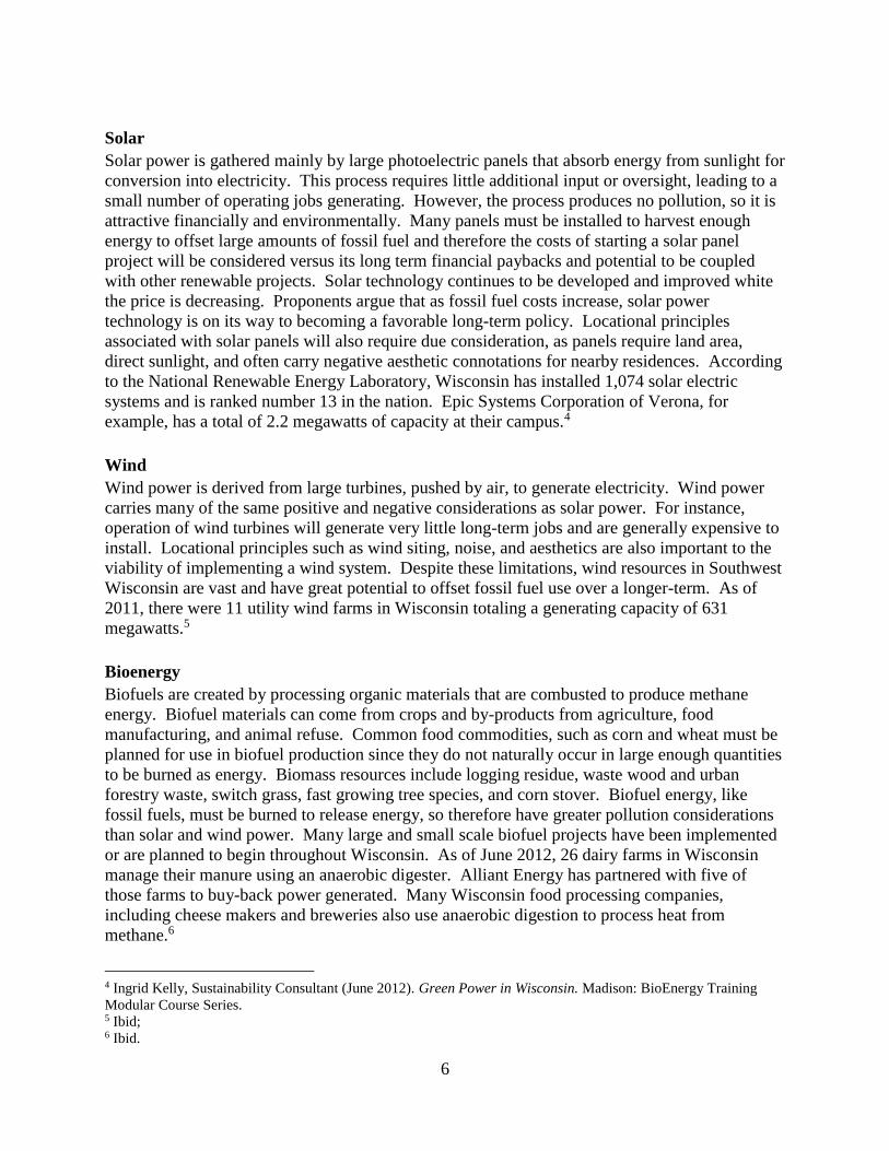
C. Renewable Energy Types This project assessed the economic potential of three types of renewable energy: solar, wind, and
bioenergy, including biomass and biogas. Work and research conducted in phase two included
review of energy consumption and renewable energy potentials and assessed the level at which
renewable energy sources could meet consumption of traditional energy sources. That said, it
behooves us to review the fundamentals of each renewable energy type discussed throughout the
assessment.
1 Region Profile, Southwest Wisconsin Regional Planning Commission, Accessed April 25, 2013.
http://swwrpc.org/wordpress/region/ 2Occupational Employment Statistics. Bureau of Labor Statistics, U.S. Department of Labor. Accessed October 13,
2011.http://www.bls.gov/oes/current/oes_5500004.htm 3 American FactFinder. U.S. Census Bureau. Accessed October 11, 2011. http://factfinder2.census.gov
6
Solar
Solar power is gathered mainly by large photoelectric panels that absorb energy from sunlight for
conversion into electricity. This process requires little additional input or oversight, leading to a
small number of operating jobs generating. However, the process produces no pollution, so it is
attractive financially and environmentally. Many panels must be installed to harvest enough
energy to offset large amounts of fossil fuel and therefore the costs of starting a solar panel
project will be considered versus its long term financial paybacks and potential to be coupled
with other renewable projects. Solar technology continues to be developed and improved white
the price is decreasing. Proponents argue that as fossil fuel costs increase, solar power
technology is on its way to becoming a favorable long-term policy. Locational principles
associated with solar panels will also require due consideration, as panels require land area,
direct sunlight, and often carry negative aesthetic connotations for nearby residences. According
to the National Renewable Energy Laboratory, Wisconsin has installed 1,074 solar electric
systems and is ranked number 13 in the nation. Epic Systems Corporation of Verona, for
example, has a total of 2.2 megawatts of capacity at their campus.4
Wind
Wind power is derived from large turbines, pushed by air, to generate electricity. Wind power
carries many of the same positive and negative considerations as solar power. For instance,
operation of wind turbines will generate very little long-term jobs and are generally expensive to
install. Locational principles such as wind siting, noise, and aesthetics are also important to the
viability of implementing a wind system. Despite these limitations, wind resources in Southwest
Wisconsin are vast and have great potential to offset fossil fuel use over a longer-term. As of
2011, there were 11 utility wind farms in Wisconsin totaling a generating capacity of 631
megawatts.5
Bioenergy
Biofuels are created by processing organic materials that are combusted to produce methane
energy. Biofuel materials can come from crops and by-products from agriculture, food
manufacturing, and animal refuse. Common food commodities, such as corn and wheat must be
planned for use in biofuel production since they do not naturally occur in large enough quantities
to be burned as energy. Biomass resources include logging residue, waste wood and urban
forestry waste, switch grass, fast growing tree species, and corn stover. Biofuel energy, like
fossil fuels, must be burned to release energy, so therefore have greater pollution considerations
than solar and wind power. Many large and small scale biofuel projects have been implemented
or are planned to begin throughout Wisconsin. As of June 2012, 26 dairy farms in Wisconsin
manage their manure using an anaerobic digester. Alliant Energy has partnered with five of
those farms to buy-back power generated. Many Wisconsin food processing companies,
including cheese makers and breweries also use anaerobic digestion to process heat from
methane.6
4 Ingrid Kelly, Sustainability Consultant (June 2012). Green Power in Wisconsin. Madison: BioEnergy Training
Modular Course Series. 5 Ibid; 6 Ibid.

7
D. AURI and JEDI Models
AURI: Determining the Economic Viability of Renewable Energy Systems
Determining Renewable Energy Potential
In order to determine the energy potential of the region, we employed the Template for the
Estimating County Level Energy Use and Renewable Energy Potential, a model developed by
the Agricultural Utilization Research Institute (AURI). This model was designed to calculate two
things: one, the annual energy use of a given county, and two, the annual technical potential of
renewable energy sources on a county level. By energy potential, we mean the technical capacity
of the region to accommodate renewable energy sources based on local land uses, system
capacity, and geographic constraints. The technical potential is generally used as an upper limit
on the amount of energy that can be produced. It does not account for the economic feasibility of
the project nor the market potential based upon policies and incentives which influence the
development of renewable energy sources. Both outputs are described in trillion BTUs. We
applied this model to each of the five counties in order to determine what percentage of each
county’s energy use could potentially be replaced energy from renewable sources produced
within the county.
In order to calculate bioenergy potential, we needed to derive data for crop residue, animal
residue, and forest wastes and residues. We used data from the U.S. Census, the USDA Census
of Agriculture, and the U.S. Forest Service in order to determine the amount of material available
for the production of renewable energy in each county. For wind, we determined the number of
acres available to have wind farms on them. AURI recommends that users treat solar as a
potential replacement of commercial or residential heating, and it suggests that they calculate the
number of BTUS created generated by solar based on a conservative estimate of the percentage
of these heating costs that might be converted to solar.
Assumptions Made in Calculating Potential
These estimates were accompanied by a series of assumptions. For example, we knew that while
a lot of land is physically able to accommodate wind turbines, there are many reasons that wind
turbines will not be installed in some of the available locations (lack of interest in wind,
opposition by neighbors, aesthetic concerns, etc.). Thus, we used conservative estimates of the
land available for the wind energy, estimating that 5% of land available to wind turbines would
actually build turbines. Due to the fact that wind power is only generated when the wind is
blowing, we also assumed that the turbines would only produce energy 25% of the time over the
8
course of a year. In addition, AURI recognizes that not all residues available would be used for
renewable energy production, and therefore the model included some built-in assumptions in this
regard. For crop residue, the model follows conservation tillage practices, meaning a portion of
the crop residues are left on the field. In this case, the model assumes that 50% of total corn
stover is removed from the field and that 75% of all other crops are removed. The model also
assumes that 100% of animal waste will be removed. In counties that have logging, the model
assumes that 33% of the available logging residues are used for renewable energy.
Determining Current Energy Use
Each group estimated the energy use by sector within its county in order to calculate the total
energy use by county. The model allows the user to input residential, transportation, agricultural
(on-farm), industrial, and commercial use. We used data from the U.S. Census, the Wisconsin
DOT, and the USDA Census of Agriculture to determine our inputs for each sector.
Limitations of Calculating Current Energy Use
Estimates of commercial energy use are a challenge with this particular model, because no good
database exists to estimate the commercial space in a city, county, or region. (Some information
is available through local property tax records, but these hard to find and extremely time
consuming to compile for a large region.) AURI acknowledges this deficiency, recommending
that users estimate the energy use for individual buildings in the region.7 Because only one of our
groups was able to calculate commercial energy use, we decided to omit commercial energy
from our analysis.
The model does not address energy conservation since the model is focused on renewable energy
as it relates to economic development planning. This is something a planner focused on reducing
a community’s dependency on nonrenewable energy sources may wish to explore further.
Assumptions Made in Calculating Energy Use
The AURI model was built on a series of assumptions. For example, when using the AURI
models, energy used for agricultural purposes is calculated from the acres in production by type
of crop or the number of livestock within a county. The model utilizes an average amount of
diesel, gasoline, LP gas, and electricity (kW/hr) per unit for each of these categories which
contribute to the total agricultural energy usage.8 Diesel is the primary form of agricultural
energy consumption, which is highly reflective of the equipment used to grow agricultural crops
and transport it to storage facilities. We averaged the energy use over a ten-year time period in
7 6Solutions, “Template for Estimating County Level Energy Use and Renewable Energy Potential,” Agricultural
Utilization Research Institute (2009). http://bit.ly/1291mcF 8 These calculations are based off of Barry, Ryan and Douglas G. Tiffany. “Minnesota Agricultural Energy Use and
the Incidence of a Carbon Tax” Minnesotans for an Energy Efficient Economy, April 1998. The values are
primarily to be used as estimates due to increased technology that should have resulted in more efficient farming
practices.
9
order to estimate the likely energy use in a single year. Additional built-in assumptions are
detailed in the AURI Template Model which can be found on their website.
JEDI: Determining the Economic Impact and Job Creation
In estimating the economic impact of renewable energy projects in the five-county region, we
used the JEDI Model, which was developed by the National Renewable Energy Laboratory. The
JEDI model was designed to evaluate the economic development potential of wind, biofuels
(such as biodiesel), solar, natural gas, coal, marine, hydrokinetic, and geothermal projects. Users
input project specifications project and costs, and the model estimates economic impact on the
local economy. The output includes direct, indirect, and induced impacts as well as the number
of jobs created during construction and jobs required annually, post-construction. We used the
JEDI model to evaluate the economic potential of solar photovoltaic and wind energy projects.
We collected case studies we collected from throughout the Upper Midwest, and we used the
specifications of these example projects to estimate reasonable inputs to use with the model.
Case studies ranged from .6 MW to 162 MW, from small pilot projects to utility-sized projects,
and we ran the model with projects of varying sizes.
JEDI models are not available for bioenergy projects (biogas and biomass). We researched an
array of existing projects throughout the state to derive information regarding the economic
impact or feasibility of these types of projects. The case studies take into account a variety of
feedstock options, ownership arrangements, and generate various sources of energy.
Limitations
Like all input-output models, JEDI results are estimates, not precise forecasts. There are a lot of
reasons why the results generated by JEDI do not perfectly predict the economic impact of a
renewable energy project. First of all, JEDI reports only the direct impact of a specific project. It
does not take into account other economic impacts that could occur as a result of these projects
being implemented. For example, the model does not factor in the fact that new investments in
renewable energy may impact electrical rates. Money spent on a wind farm could have been
spent on something else (opportunity cost), and the model does not estimate what economic
impact this altered spending pattern would have. In addition, the model does not take into
account economies of scale that could be created by having more renewable energy projects in
one place. The cost of a ten wind farms is simply the cost of one wind farm multiplied by ten.
Because of this, prices do not change with demand.
It is important to note that this is a state-based economic analysis. The model was developed
based on relationships between industries at a state level. Since our area of focus was at the
county level, we input the population of each particular county as a proxy for the state
population. However, the model estimates the local share of the economy relative to the state and
may not reflect the actual industry base of the county in question. For example, the model may
predict that a renewable energy project will have an impact on an industry that does exist in the
county of study. Thus, the model’s estimated economic impacts must be taken with a grain of
10
salt. Finally, the model does not consider the economic viability or profitability of projects. It
assumes that owners of renewable energy projects have determined that the project is financially
viable before construction.
These are the considerations that were the most relevant to our analysis. The National Renewable
Energy Laboratory provides a complete list of the limitations of their JEDI model on their
website.9 These limitations are generally true for all input-output models, and so it does not
necessarily mean JEDI is a weak model. As long as the user understands these limitations and
uses the model for the right purposes, he or she should be able to make reasonable estimates of
the economic impacts of renewable energy projects.
Assumptions
When creating the JEDI model, the of JEDI had to make judgments in fitting renewable energy
technologies into the fixed categories defined by the North American Industry Classification
System, some of which may not have been perfect matches. In addition, the results are based on
the basic assumption that factors of production and industrial inputs are used in fixed proportions
and respond perfectly elastically. In other words, the economic impacts are linearly related to the
size of the project without regard to potential economies of scale. Thus, a 10 MW project will
have twice the impact of a 5 MW project, even though savings may have accrued through
economies of scale. For smaller projects, this is a minor issue, but for larger projects, economic
impacts may be overstated. The JEDI model also has certain built-in assumptions, which we did
not alter. JEDI’s default assumptions are based on industry averages.
Data The data from the AURI models can be found in the appendices at the end of the report. They
show the different input and output tables and the numerical assumptions used by the model.
Appendix A tabulates the renewable energy potential of each county. Each county has a table
for total energy potential, potential from crop residue, methane from livestock, logging residue
(if applicable), and wind energy potential. Appendix B has the AURI tables for the estimated
energy use for each county. These tables include estimated annual energy use, as well as break
downs for residential, industrial, transportation, and agriculture uses.
Discussion In this section, we examine each county’s energy consumption and each counties renewable
energy potential. The unit for these measurements is in megawatt hours annually. We will also
estimate each county’s megawatt potential for wind, agriculture crop residue, livestock residue,
and logging residue. Finally, in an effort to provide a region outlook, we’ve aggregated each
county’s energy consumption and renewable energy potential.
9 http://www.nrel.gov/analysis/jedi/limitations.html

11
Although we looked at each counties residential, transportation, agricultural, and industrial
energy use, we are only factoring each county’s residential and industrial energy use when
comparing it to the renewable energy potential of wind, agriculture crop residue, livestock
residue, and logging residue. This strategic decision is based in large part on the notion that the
renewable energy potential of natural resources like wind, agriculture crop residue, livestock
residue, and logging residue are most suited to offset current residential and industrial energy use
and not, for instance, the diesel and gas energy consumption embedded in transportation and
certain agriculture activities.
E. County and Regional Outlook
1. Iowa County
Iowa appears to have a surplus of renewable energy relative to its current industrial and
residential energy use (Figure 3). The annual industrial and residential energy consumption is
below 2 million megawatt hours while the annual renewable energy potential hovers around 3
million megawatt hours.
Figure 1: Iowa renewable energy v. energy consumption
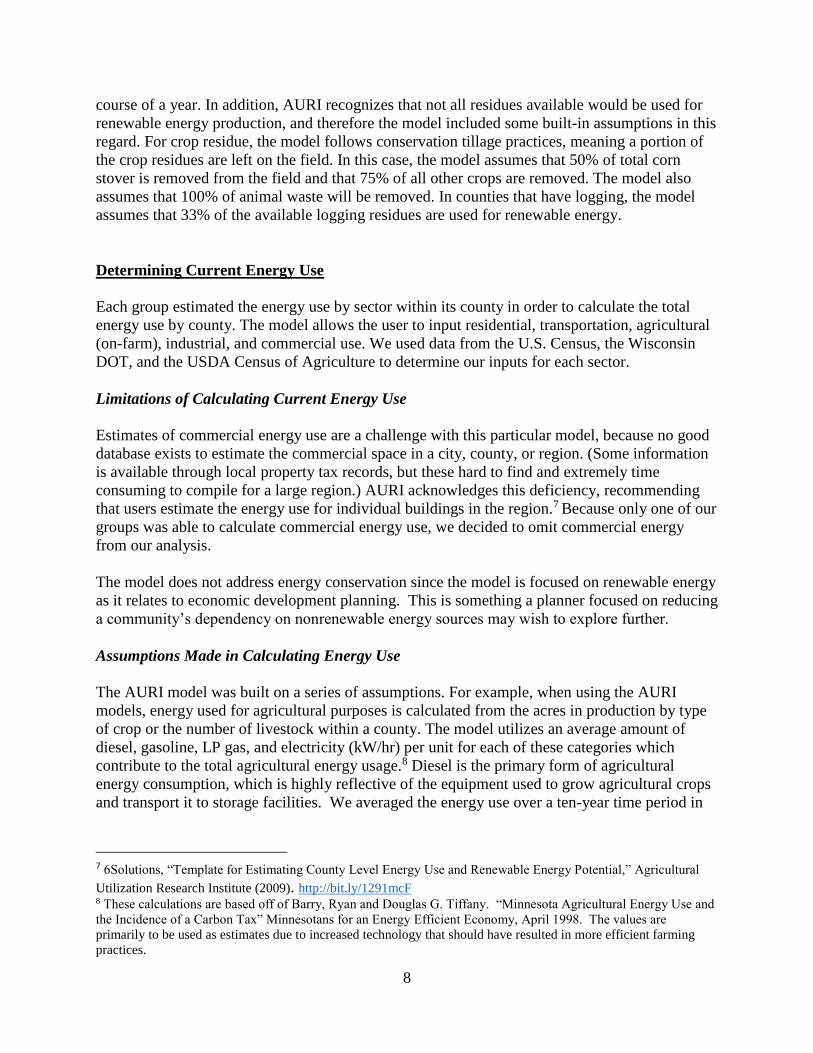
In terms of energy consumption, figure 4 illuminates the current residential, transportation,
agricultural, and industrial energy consumption throughout the county. Interestingly,
transportation accounts for the majority of the energy use in Iowa County with approximately 2
million megawatt hours annually. Residential and Industrial energy consumption are a close
second, each just under 1 million megawatt hours annually.
12
Figure 2: Iowa county energy consumption
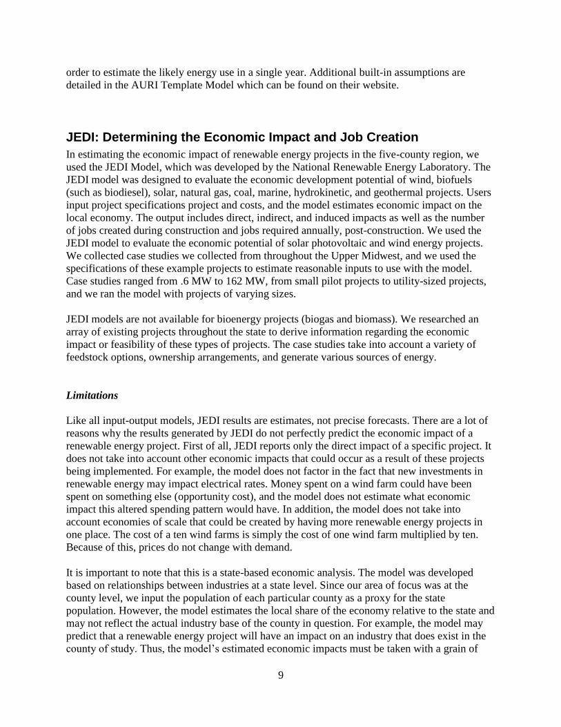
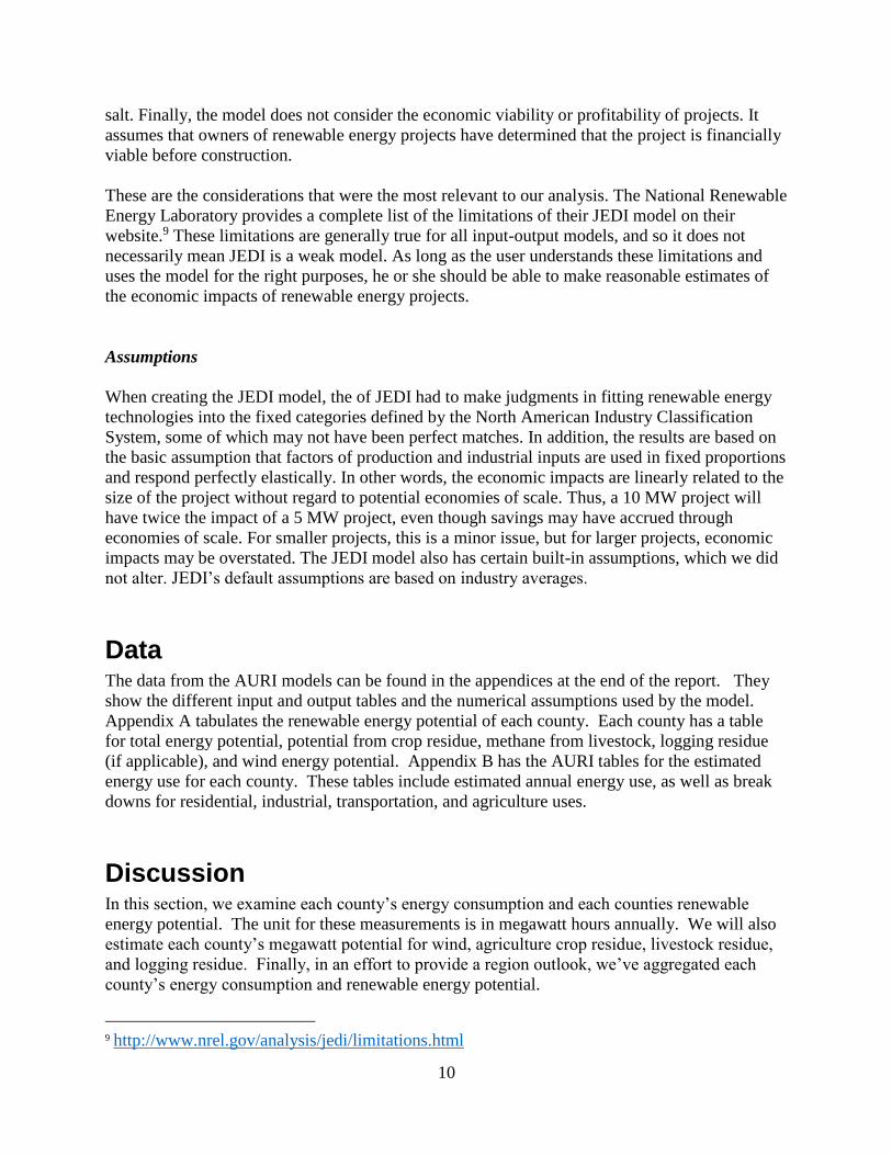
In figure 5, we see Iowa counties renewable energy portfolio. The majority of renewable energy
potential appears to come from wind. The county appears to be in a position to host up to 251
megawatts worth of wind turbines. Agricultural crop residue and livestock residue offer 89 and
15 megawatts worth of potential, respectively, while logging residue remains non-existent.
Ultimately, renewable energy potential in Iowa County is nearly twice industrial and residential
energy use.
Figure 3: Iowa county renewable energy potential (megawatts)
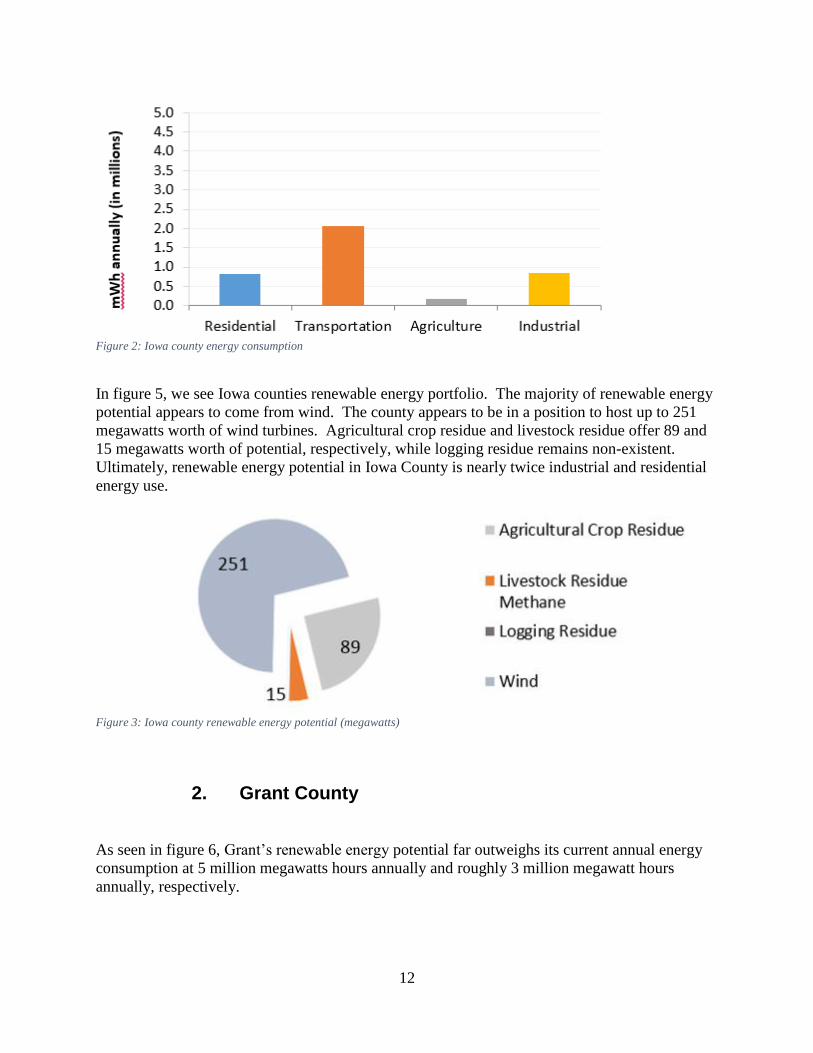
2. Grant County
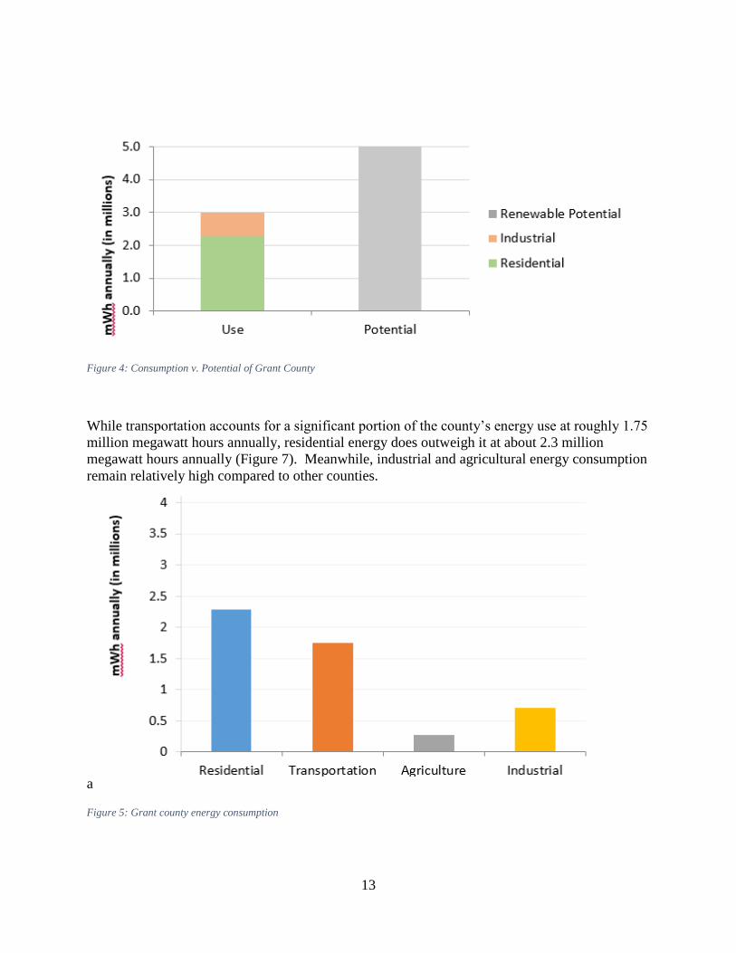
As seen in figure 6, Grant’s renewable energy potential far outweighs its current annual energy
consumption at 5 million megawatts hours annually and roughly 3 million megawatt hours
annually, respectively.
13
Figure 4: Consumption v. Potential of Grant County
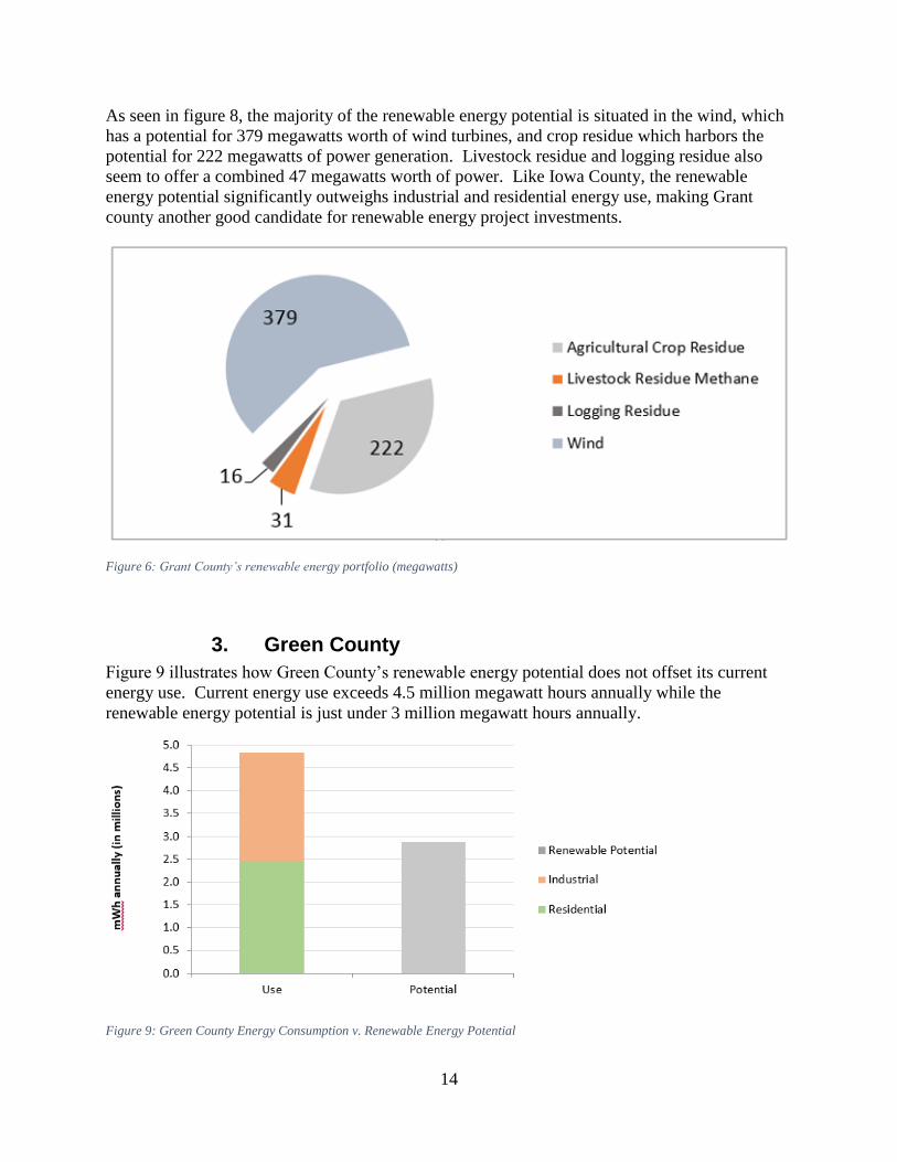
While transportation accounts for a significant portion of the county’s energy use at roughly 1.75
million megawatt hours annually, residential energy does outweigh it at about 2.3 million
megawatt hours annually (Figure 7). Meanwhile, industrial and agricultural energy consumption
remain relatively high compared to other counties.
a
Figure 5: Grant county energy consumption
14
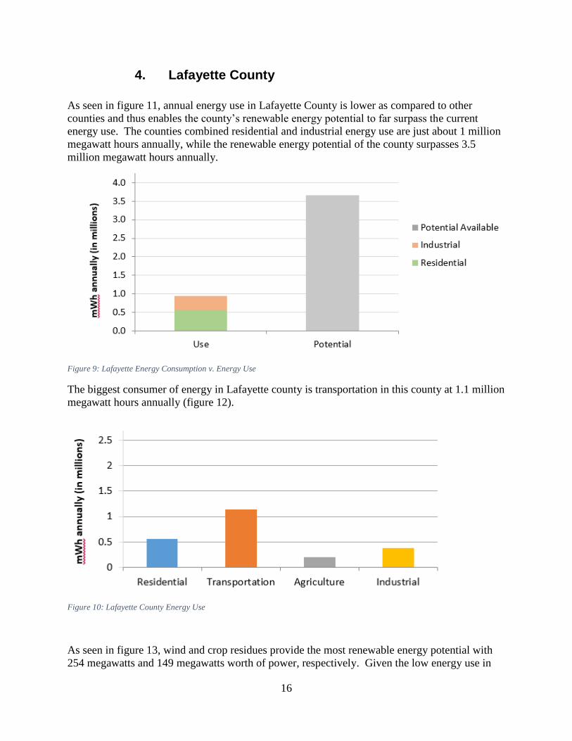
As seen in figure 8, the majority of the renewable energy potential is situated in the wind, which
has a potential for 379 megawatts worth of wind turbines, and crop residue which harbors the
potential for 222 megawatts of power generation. Livestock residue and logging residue also
seem to offer a combined 47 megawatts worth of power. Like Iowa County, the renewable
energy potential significantly outweighs industrial and residential energy use, making Grant
county another good candidate for renewable energy project investments.
Figure 6: Grant County’s renewable energy portfolio (megawatts)
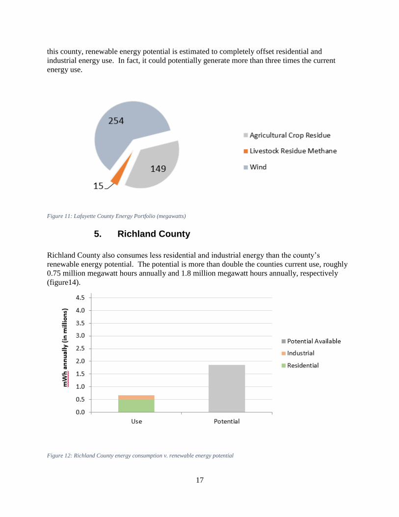
3. Green County
Figure 9 illustrates how Green County’s renewable energy potential does not offset its current
energy use. Current energy use exceeds 4.5 million megawatt hours annually while the
renewable energy potential is just under 3 million megawatt hours annually.
Figure 9: Green County Energy Consumption v. Renewable Energy Potential

15
The high energy use in Green County is in large part due to the high industrial and residential
energy use, roughly 2.4 million megawatt hours and 2.45 million megawatt hours annually,
respectively. Transportation energy consumption isn’t far behind at just over 1.75 million
megawatt hours annually (figure 10).
Figure 70: Green County's energy consumption
Although Green county is unlikely to completely offset its energy use with renewable sources of
energy, the county still demonstrates a substantial amount of megawatt worth of wind and
agricultural crop residue at 193 megawatts and 130 megawatts, respectively. That said, if
pursued, this power could help offset the entire five county regions energy use (figure 9).
Figure 81: Green County's renewable energy potential portfolio (megawatts)
16
4. Lafayette County
As seen in figure 11, annual energy use in Lafayette County is lower as compared to other
counties and thus enables the county’s renewable energy potential to far surpass the current
energy use. The counties combined residential and industrial energy use are just about 1 million
megawatt hours annually, while the renewable energy potential of the county surpasses 3.5
million megawatt hours annually.
Figure 9: Lafayette Energy Consumption v. Energy Use
The biggest consumer of energy in Lafayette county is transportation in this county at 1.1 million
megawatt hours annually (figure 12).
Figure 10: Lafayette County Energy Use
As seen in figure 13, wind and crop residues provide the most renewable energy potential with
254 megawatts and 149 megawatts worth of power, respectively. Given the low energy use in
17
this county, renewable energy potential is estimated to completely offset residential and
industrial energy use. In fact, it could potentially generate more than three times the current
energy use.
Figure 11: Lafayette County Energy Portfolio (megawatts)
5. Richland County
Richland County also consumes less residential and industrial energy than the county’s
renewable energy potential. The potential is more than double the counties current use, roughly
0.75 million megawatt hours annually and 1.8 million megawatt hours annually, respectively
(figure14).
Figure 12: Richland County energy consumption v. renewable energy potential
18
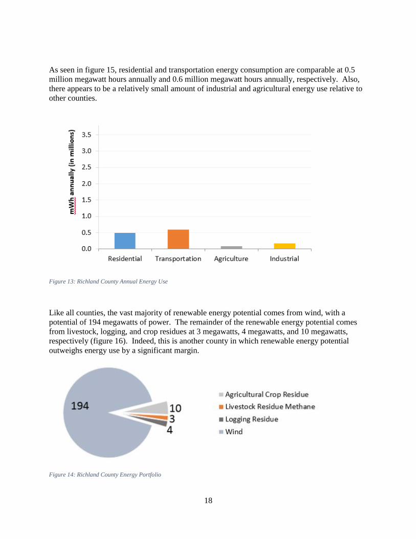
As seen in figure 15, residential and transportation energy consumption are comparable at 0.5
million megawatt hours annually and 0.6 million megawatt hours annually, respectively. Also,
there appears to be a relatively small amount of industrial and agricultural energy use relative to
other counties.
Figure 13: Richland County Annual Energy Use
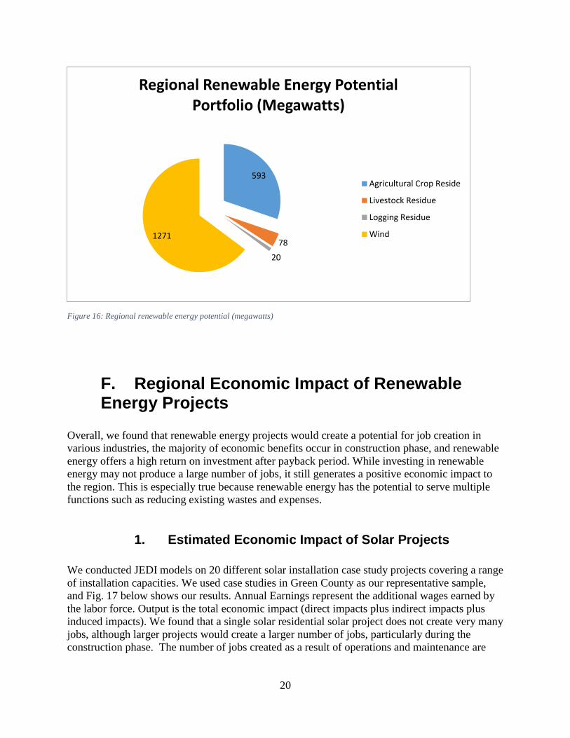
Like all counties, the vast majority of renewable energy potential comes from wind, with a
potential of 194 megawatts of power. The remainder of the renewable energy potential comes
from livestock, logging, and crop residues at 3 megawatts, 4 megawatts, and 10 megawatts,
respectively (figure 16). Indeed, this is another county in which renewable energy potential
outweighs energy use by a significant margin.
Figure 14: Richland County Energy Portfolio

19
6. Summary: Regional Outlook
As seen in figure 15, an aggregate of each counties data indicates that there is enough technical
potential in the five-county area to offset the region’s total estimated annual industrial and
residential energy use. This is a significant offset, which may suggest that renewable energy
projects would be a viable option should the region seek to pursue energy independence. Even
though potential renewable energy did not offset current residential and industrial use in Green
County, the totality of the other four counties renewable energy surplus offsets Green County’s
deficits. Overall, we can conclude that the total potential for renewable energy in this region is
considerable.
Figure 15: Regional energy consumption v. energy potential (million megawatt hours annually)
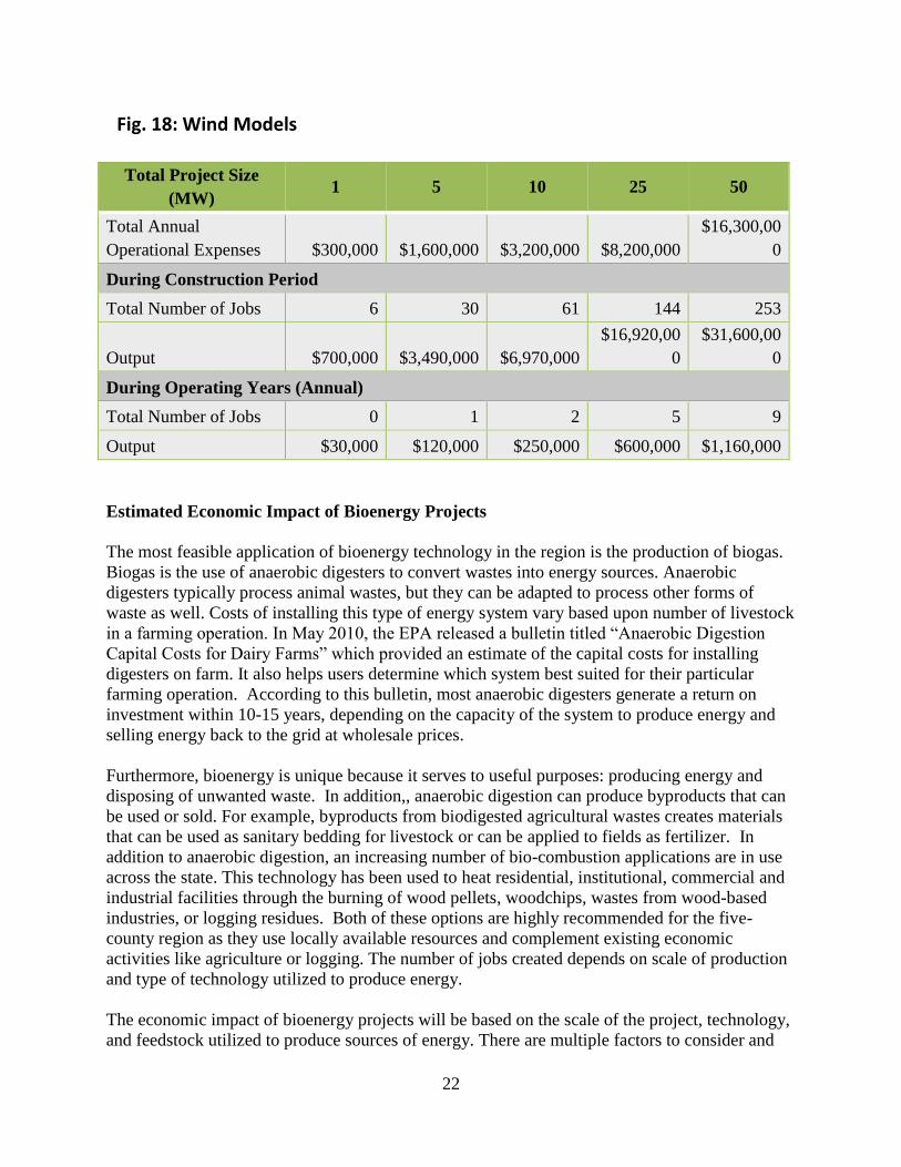
Figure 16 illustrates that the aggregation of each counties renewable energy portfolio indicates
that wind is the primary generator of renewable energy potential at 1271 megawatts worth of
power. Crop residue, livestock residue and logging residue also provide potential power, at 593
megawatts, 78 megawatts, and 20 megawatts, respectively.
20
Figure 16: Regional renewable energy potential (megawatts)
F. Regional Economic Impact of Renewable Energy Projects
Overall, we found that renewable energy projects would create a potential for job creation in
various industries, the majority of economic benefits occur in construction phase, and renewable
energy offers a high return on investment after payback period. While investing in renewable
energy may not produce a large number of jobs, it still generates a positive economic impact to
the region. This is especially true because renewable energy has the potential to serve multiple
functions such as reducing existing wastes and expenses.
1. Estimated Economic Impact of Solar Projects
We conducted JEDI models on 20 different solar installation case study projects covering a range
of installation capacities. We used case studies in Green County as our representative sample,
and Fig. 17 below shows our results. Annual Earnings represent the additional wages earned by
the labor force. Output is the total economic impact (direct impacts plus indirect impacts plus
induced impacts). We found that a single solar residential solar project does not create very many
jobs, although larger projects would create a larger number of jobs, particularly during the
construction phase. The number of jobs created as a result of operations and maintenance are
593
78
20
1271
Regional Renewable Energy Potential Portfolio (Megawatts)
Agricultural Crop Reside
Livestock Residue
Logging Residue
Wind

21
minimal regardless of the scale of the project; however, they do produce a small induced impact
on the economy.
Residential
Retrofit
(1 System)
Residential Retrofit
(100 Systems)
Large
Commercial Utility
During Construction and Installation Period
Total Jobs 0.5 45.6 17.9 77.3
Total Earnings $157,000 $1,569,600 $628,000 $2,482,400
Total Output $498,000 $4,984,700 $1,938,600 $8,050,800
During Operation Period
Annual Jobs 0.0* 0.3 0.1 0.6
Annual Earnings $1,000 $139,000 $37,000 $26,400
Annual Output $3,000 $270,000 $70,000 $62,500
Based on the solar case studies, we learned that there would likely be more than one residential
solar project installed within a region during a given timeframe, increasing the economic impact.
We chose a representative example of one residential system, 100 residential systems, a large
commercial system, and a utility solar project to demonstrate the ability of solar applications to
generate an economic impact within the region.
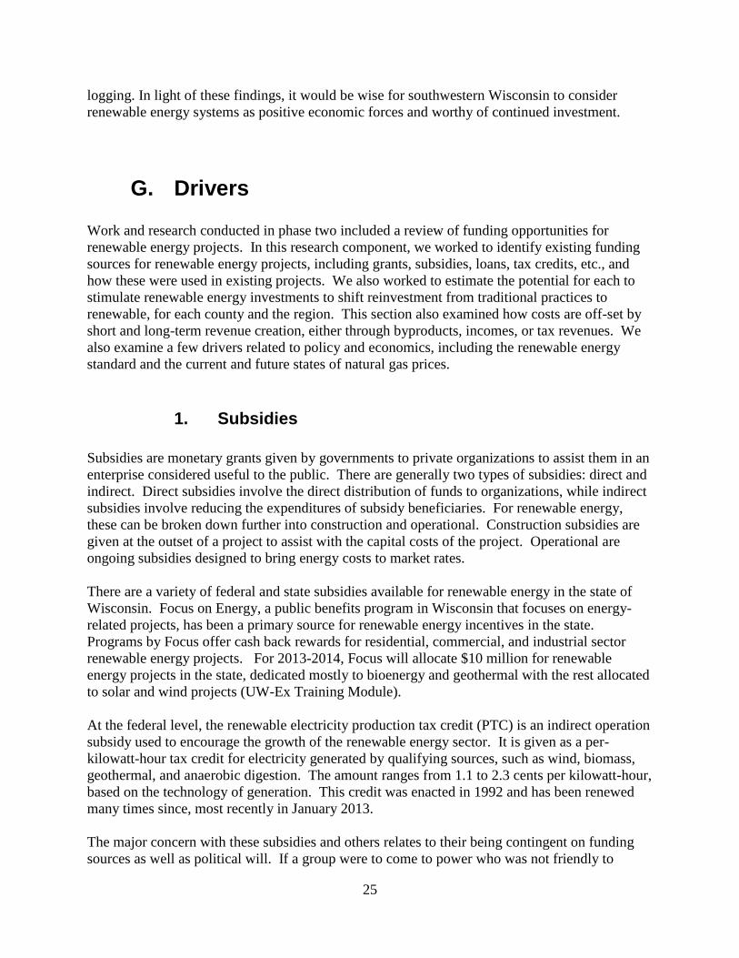
2. Estimated Economic Impact of Wind Projects
The results of our wind analysis are very similar to the solar results. We ran 20 JEDI models on
existing wind projects throughout Wisconsin and the upper Midwest. Our results, found in Fig.
18, were reached by using the default settings of the JEDI model which are based on industry
averages. This table demonstrates the economic impact of wind projects using varying scales,
while holding all other project related costs at a constant. Our findings suggest that wind
projects have the potential to generate greater economic impact than that of solar, but this is
strongly dependent on the scale of the project. As for solar, the majority of the jobs created occur
during the development and construction phase. Yet these short-term workers have the potential
to have a significant impact on the local economy during their relatively brief time in the area.
The table below shows our results for wind projects.
Fig. 17: Solar Models
*Marginal, rounds to zero.
22
Total Project Size
(MW) 1 5 10 25 50
Total Annual
Operational Expenses $300,000 $1,600,000 $3,200,000 $8,200,000
$16,300,00
0
During Construction Period
Total Number of Jobs 6 30 61 144 253
Output $700,000 $3,490,000 $6,970,000
$16,920,00
0
$31,600,00
0
During Operating Years (Annual)
Total Number of Jobs 0 1 2 5 9
Output $30,000 $120,000 $250,000 $600,000 $1,160,000
Estimated Economic Impact of Bioenergy Projects
The most feasible application of bioenergy technology in the region is the production of biogas.
Biogas is the use of anaerobic digesters to convert wastes into energy sources. Anaerobic
digesters typically process animal wastes, but they can be adapted to process other forms of
waste as well. Costs of installing this type of energy system vary based upon number of livestock
in a farming operation. In May 2010, the EPA released a bulletin titled “Anaerobic Digestion
Capital Costs for Dairy Farms” which provided an estimate of the capital costs for installing
digesters on farm. It also helps users determine which system best suited for their particular
farming operation. According to this bulletin, most anaerobic digesters generate a return on
investment within 10-15 years, depending on the capacity of the system to produce energy and
selling energy back to the grid at wholesale prices.
Furthermore, bioenergy is unique because it serves to useful purposes: producing energy and
disposing of unwanted waste. In addition,, anaerobic digestion can produce byproducts that can
be used or sold. For example, byproducts from biodigested agricultural wastes creates materials
that can be used as sanitary bedding for livestock or can be applied to fields as fertilizer. In
addition to anaerobic digestion, an increasing number of bio-combustion applications are in use
across the state. This technology has been used to heat residential, institutional, commercial and
industrial facilities through the burning of wood pellets, woodchips, wastes from wood-based
industries, or logging residues. Both of these options are highly recommended for the five-
county region as they use locally available resources and complement existing economic
activities like agriculture or logging. The number of jobs created depends on scale of production
and type of technology utilized to produce energy.
The economic impact of bioenergy projects will be based on the scale of the project, technology,
and feedstock utilized to produce sources of energy. There are multiple factors to consider and
Fig. 18: Wind Models

23
economic impact will be impacted by decisions made by a single individual, business, or farming
operation. Due to this fact, it is hard to simply summarize the economic impact of these projects.
Of the many case studies we identified, we found the following to be the most instructive and
worthy of further consideration:
Xcel Energy Bay Front Plant
Vesper Pallet Company and Woodruff Lumber
Barron Area School District
Action Floor Systems, LLC
Flambeau River Paper Mill and Flambeau River Biofuels
French Island Generating Station
Wild Rose Dairy
Janesville Wastewater Treatment Facility
Emerald Dairy Biodigester
3. The Economic Impact of One Additional Job
In addition to calculating the economic impact of the renewable energy system itself, we also
sought to identify the distribution of these economic impacts as they would occur in the region
based on local spending patterns and interrelated industries. We ran two IMPLAN models that
reflect two different income levels of an additional worker within the community. We assumed
that the worker would earn between $30,000 and $50,000 per year; the upper limit was suggested
by the JEDI models and the lower value provides a reasonable estimate. The following chart is a
breakdown of the economic impacts to various sectors of the local economy as estimated by the
JEDI model. Based on the increased amount of money in the local economy, the induced
spending is most likely to be spent on healthcare, housing, and retail – this primarily reflects that
individuals are going to pay off existing debts such as their medical bills and mortgages and act
as rational consumers to purchase the goods and services that they either want or need.
Fig. 19: Induced Impacts
Leasing

24
4. Economic Tradeoffs
It is important to consider the economic tradeoffs of investing in renewable energy projects
against the potential loss of crop income. This is a particular issue with wind turbines, as the
footprint of the turbine reduces the total amount of land that can support income-producing
crops. We calculated this tradeoff and determined that the income from energy produced by the
turbine would easily surpass the crop loss. The wind turbine would pay for itself in less than 20
years. After 20 years, I would be making a profit equivalent to growing either corn or soybeans
for over 100 years in the turbine’s footprint. The estimated loss of crop income is based on the
regional average yields in bushels per acre for corn and soybeans, USDA season average prices,
and NREL’s estimated size of a turbine footprint and standard service road. The production and
potential of a wind turbine is based on the following assumptions: the turbine produces energy
25% of the time (a conservative estimate), the buy-back price by the utility is $0.05 (a low
estimate), and that the cost of installation is $2,000 per KW (the industry standard). Our estimate
does not account for operation and maintenance costs; nor does it include any subsidies or grants
that help pay for the installation.
Significantly, this estimate does not take into account the fact that wind turbines disrupt the usual
paths of farming implements, and farmers have to take special efforts to navigate around them.
Further research is necessary to determining the optimal siting of wind turbines on a given parcel
in order to minimize possible negative economic effects that erode the benefits of building a
wind turbine.
5. Additional Sources of Income
In addition to the effects projected by JEDI and IMPLAN, there are other economic factors to
consider. For example, owners of renewable energy projects can earn additional income by
selling surplus renewable energy to utility companies. Although wholesale prices are lower than
consumer prices, they present a great opportunity for renewable energy projects to generate
income that can be used to pay for loans on the initial investment as well as ongoing operation
and maintenance costs. The return on investment is the highest for wind and agriculturally based
anaerobic digesters. Additionally, the byproducts created from biogas production can be sold, as
discussed previously.
6. Summary – Economic Opportunity
While the number of jobs produced through the installation of renewable solar, wind or
bioenergy projects is not large, these projects still have a positive economic impact on their local
communities. The jobs that are created, mainly in the construction phases, have important effects
on the local economy. Furthermore, these projects yield additional sources of income through the
sale of surplus energy and/or byproducts from the biodigestion process. Bioenergy also has the
added benefit of finding a productive use for wastes created through the process of farming or
25
logging. In light of these findings, it would be wise for southwestern Wisconsin to consider
renewable energy systems as positive economic forces and worthy of continued investment.
G. Drivers
Work and research conducted in phase two included a review of funding opportunities for
renewable energy projects. In this research component, we worked to identify existing funding
sources for renewable energy projects, including grants, subsidies, loans, tax credits, etc., and
how these were used in existing projects. We also worked to estimate the potential for each to
stimulate renewable energy investments to shift reinvestment from traditional practices to
renewable, for each county and the region. This section also examined how costs are off-set by
short and long-term revenue creation, either through byproducts, incomes, or tax revenues. We
also examine a few drivers related to policy and economics, including the renewable energy
standard and the current and future states of natural gas prices.
1. Subsidies
Subsidies are monetary grants given by governments to private organizations to assist them in an
enterprise considered useful to the public. There are generally two types of subsidies: direct and
indirect. Direct subsidies involve the direct distribution of funds to organizations, while indirect
subsidies involve reducing the expenditures of subsidy beneficiaries. For renewable energy,
these can be broken down further into construction and operational. Construction subsidies are
given at the outset of a project to assist with the capital costs of the project. Operational are
ongoing subsidies designed to bring energy costs to market rates.
There are a variety of federal and state subsidies available for renewable energy in the state of
Wisconsin. Focus on Energy, a public benefits program in Wisconsin that focuses on energy-
related projects, has been a primary source for renewable energy incentives in the state.
Programs by Focus offer cash back rewards for residential, commercial, and industrial sector
renewable energy projects. For 2013-2014, Focus will allocate $10 million for renewable
energy projects in the state, dedicated mostly to bioenergy and geothermal with the rest allocated
to solar and wind projects (UW-Ex Training Module).
At the federal level, the renewable electricity production tax credit (PTC) is an indirect operation
subsidy used to encourage the growth of the renewable energy sector. It is given as a per-
kilowatt-hour tax credit for electricity generated by qualifying sources, such as wind, biomass,
geothermal, and anaerobic digestion. The amount ranges from 1.1 to 2.3 cents per kilowatt-hour,
based on the technology of generation. This credit was enacted in 1992 and has been renewed
many times since, most recently in January 2013.
The major concern with these subsidies and others relates to their being contingent on funding
sources as well as political will. If a group were to come to power who was not friendly to

26
renewable energy, then subsidies such as the ones mentioned above could be greatly reduced or
done away with altogether. During times of economic downturn, those subsidies might be also
be subject to budget cuts.
2. Renewable Energy Standard
The Renewable Energy Standard is a policy instrument that aims to increase the production of
electricity from renewable energy sources with desirable social and environmental benefits. The
RES requires the market to deliver a set minimum percentage of renewable electricity generation
or capacity requirement from targeted fuels or technologies. There is also a deadline dictated as
to when this minimum percentage must be reached, i.e. 20% by the years 2020. The RES has
emerged as a popular mechanism to increase the penetration of renewables into the electricity
market. Renewable fuel sources included in RES policy typically include solar, wind, geothermal
heat, hydroelectric, and bioenergy. Renewables usually have much lower social and
environmental impacts, compared to electricity derived from conventional sources.
Environmental benefits might be local—less smog contributing emissions—or global—reduced
emissions of greenhouse gases. Investing in renewables also increases supply diversity, making
energy systems less vulnerable to changing fuel prices or disruptions in the supply chain (Berry
& Jaccard, 2006).
Despite notable environmental and societal implications of renewable energy, there is still debate
as to whether it is more expensive than conventional electricity sources when compared on a
financial cost basis. Traditionally, utilities have concentrated their investments on conventional
technologies, such as coal and natural gas power plants, which tend to have lower capital, fuel
and operations and maintenance costs. The RES addresses this problem by mandating that
utilities generate or purchase a certain amount of electricity from renewable as a portion of their
overall electricity supply. Additionally, many state officials view the RES as a way to respond to
public demand for reliable, inexpensive, and environmentally friendly source of electricity.
Another factor that contributes to diverse support of the RES is the perception that promoting
renewable energy through these standards produces economic benefits for the state, in the form
of economic development. Development is particularly attractive if the renewable sources are
developed within state boundaries, in lieu of imported fossil fuels (Rabe, 2007, p. 10).
One of the main challenges of the RES is determining the target or quota. Wisconsin approached
the issue of integrating renewable source in a two-step manner. In 1998, state passed legislation
used a fixed 50-megawatt renewable capacity target for a portion of the state, with mandated
completion by 2000. In 1999, the state enacted a second RES, applicable to the entire state,
which required that at least .5 percent of the electricity sold in 2001—increasing to 2.2 percent
by 2011—be derived from renewable sources. In 2006, Wisconsin increased RES to 10 percent
by 2015, which is where it currently stands. Under the Wisconsin state law, there are a range of
technologies and eligible resources: tidal or wave power, wind power, solar photovoltaic,
geothermal activity, fuel cell using renewable fuel (as determined by the PSC), hydroelectric,
and biomass. Exclusions consist of energy deriving from coal, oil, nuclear, or natural gas (except
for natural gas used in a fuel cell). Under current law, electric utilities are permitted to recover
the costs of providing renewable energy generation that equal or exceed the RES requirements

27
using alternative price structures, which include asking customers pay a premium for using
electricity generated through renewable resources.
Wisconsin is well on its way to meeting the 2015 goal; however it is difficult to assume that
those electric utility companies will continue to invest in renewable energies beyond their
mandated levels of compliance. Other states have begun to raise the bar for the amount of
electricity required by an RES, which has resulted in somewhat of a “race to the top,” where
states are committing to renewable energy levels that might not have seemed fathomable a
decade ago (Rabe, 2007, p.15). Additionally, state RES programs are increasingly complemented
by other initiatives to promote renewable energy and energy efficiency, such as third party solar
programs. The RES serves as an important policy tool, encouraging a commitment to renewable
energy, by both markets and consumers. It remains unseen whether legislative action will be
taken to increase or extend the state’s RES.
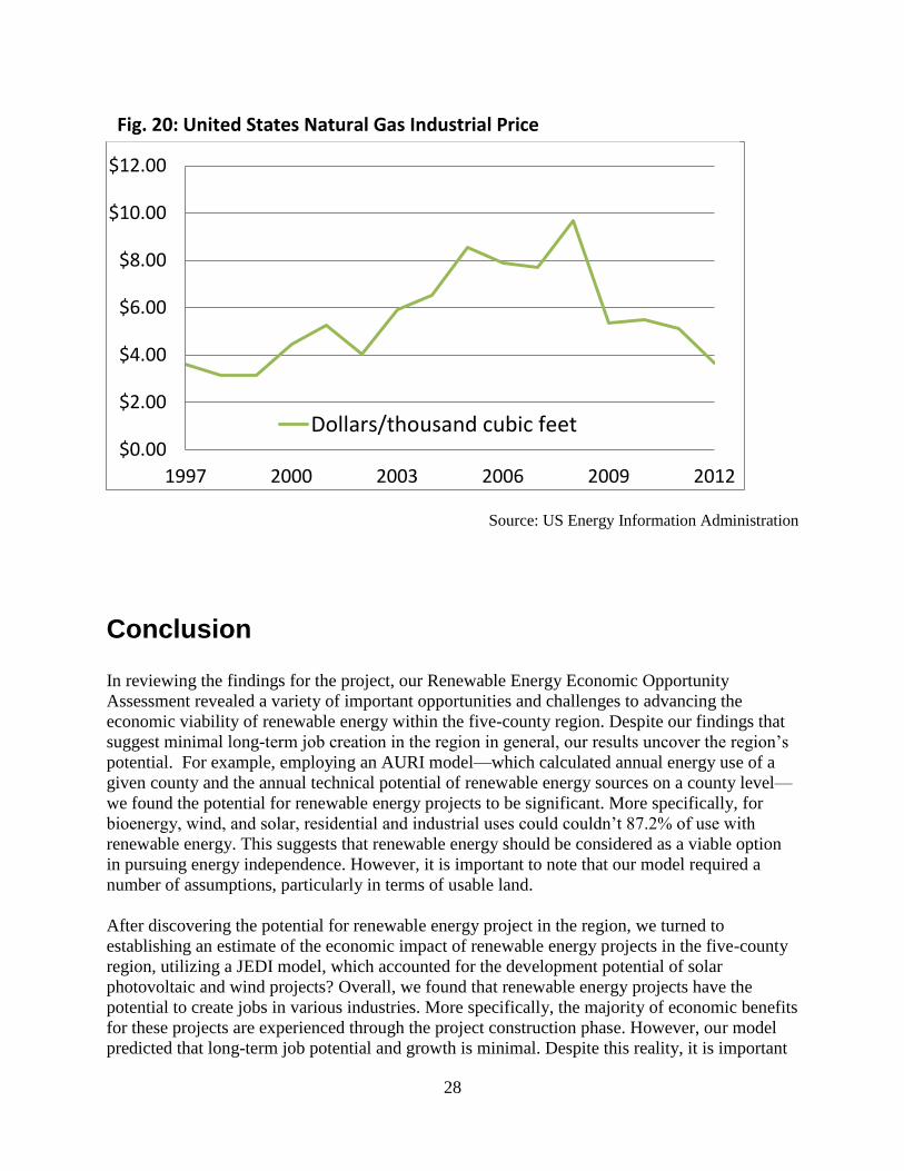
3. Natural Gas
Another contributing driver that we consider in our analysis of renewable energy potential in
Southwestern Wisconsin is the role of decreasing North American gas prices, as shown in figure
20. Estimates find that demand for natural gas will increase significantly over the next decade,
given the rapid rise of domestic production (Navigant, “North American Natural Gas Market
Outlook, Fall 2012). New drilling technologies, pioneered in America, are allowing gas to be
extracted from deposits that were formerly technologically and economically out of reach. There
is a growing awareness of natural gas as a source of domestic energy supply, with producers
seeking new markets for natural gas, such as transportation. Additionally, there is growing
recognition of the low carbon content of natural gas relative to other fossil fuels, which some
scholars say could act as a “bridge” to a low carbon future (Ejaz, p. 40).
In the short term, low natural gas prices do not appear to significantly undercut investment in
renewable energy. For example, current prices for wind, since those prices are usually based on
fixed 20-year prices, not market prices. Additionally, while the cost per kilowatt hour of wind is
more expensive than natural gas, utilities often still encourage the presence of renewable energy
in order to have a more robust portfolio of generation sources and to guard against the volatility
of natural gas prices. In the long term, if low natural gas prices persist, the political will for
renewable energy—in the form of tax subsidies for solar and wind installations—could
potentially wane. While we found a few sources that suggested that a reduction in natural gas
resources could mean less investment in renewable energy, we were unable to find substantial
literature to completely support this claim. One factor to consider is that while natural gas
produces half as much carbon dioxide per watt of power as coal, it is still a considered a “dirty
energy,” so investment for renewable energy still presents viable alternative for a clean energy
future.
28
Source: US Energy Information Administration
Conclusion
In reviewing the findings for the project, our Renewable Energy Economic Opportunity
Assessment revealed a variety of important opportunities and challenges to advancing the
economic viability of renewable energy within the five-county region. Despite our findings that
suggest minimal long-term job creation in the region in general, our results uncover the region’s
potential. For example, employing an AURI model—which calculated annual energy use of a
given county and the annual technical potential of renewable energy sources on a county level—
we found the potential for renewable energy projects to be significant. More specifically, for
bioenergy, wind, and solar, residential and industrial uses could couldn’t 87.2% of use with
renewable energy. This suggests that renewable energy should be considered as a viable option
in pursuing energy independence. However, it is important to note that our model required a
number of assumptions, particularly in terms of usable land.
After discovering the potential for renewable energy project in the region, we turned to
establishing an estimate of the economic impact of renewable energy projects in the five-county
region, utilizing a JEDI model, which accounted for the development potential of solar
photovoltaic and wind projects? Overall, we found that renewable energy projects have the
potential to create jobs in various industries. More specifically, the majority of economic benefits
for these projects are experienced through the project construction phase. However, our model
predicted that long-term job potential and growth is minimal. Despite this reality, it is important
$0.00
$2.00
$4.00
$6.00
$8.00
$10.00
$12.00
1997 2000 2003 2006 2009 2012
Dollars/thousand cubic feet
Fig. 20: United States Natural Gas Industrial Price
29
to note that there tends to be a high return on investment after the project payback period for
renewable energy projects, and projects can serve multiple functions, such as waste and expenses
reduction.
Lastly, our analysis takes into account that renewable energy projects are significantly affected
by outside sources, independent of potential or economic impact. We identified a number of
factors that may contribute to feasibility of renewable energy projects. For example, the
availability of subsidies— federal or state, indirect or direct, or during construction and operation
phase construction or operation phase— could boost or stall the number of project in the region.
However, the subsidy environment is often dependent on political will, which is often
complicated an unpredictable. Similarly, a change in Wisconsin’s Renewable Portfolio Standards
could potentially boost investment in renewable energy projects, as the market is required to
deliver a particular minimum of renewable electricity. However, as Wisconsin has nearly
reached its 2015 Renewable Portfolio Standards, and no legislation has passed that would raise
the percentage; it is unclear as to whether electric utility companies will continue to invest in
renewable energy projects. Finally, as natural gas prices drop, it becomes more appealing as
lower carbon emitting, form of energy. All of these factors should be taken into consideration
when considering the potential for renewable energy in the region.
Literature Cited
--Berry, Trent, and James Jaccard. Sustainable Production: Building Canadian Capacity.
Vancouver: UBC, 2006.
-- Rabe, Berry. "Race to the Top: The Expanding Role of U.S. Renewable Portfolio
Standards." Sustainable Development Law and Policy 10.7 (2006): 10-30. Web
-- Pickery, Gordon. "North American Natural Gas Market Outlook." Navigant Fall Update (12
Dec. 2012): 1-14. Print.
--Ejaz, Qudsia J. "The Future of Natural Gas." MIT Energy Initiative. Web. p.40. 04 Feb. 2013

30
Renewable Energy Potential
A. Grant County
1. Table 1.1: Estimated Annual Renewable Energy Potential Summary
2. Table 1.2: Estimated Annual Crop Residue Potential
Resource Quantity Units Energy ContentTrillion Btu/yr
Agricultural Crop Residue Tons 6.6336
Livestock Residue Methane SCF 0.9333
Logging Residue Tons 0.4762
Wind kW-hr 11.3232
Total 19.3663
Total Number of Households 19,396
Column B C D
Formula =household number * B
Energy Type
Million
Btu/househol
d
per year
Annual Energy
Million Btu/yrOn Site
Electricity - Primary 111.5 2,162,654.00 −−
Electricity - Site 37.3 723,470.80 723,470.80
Natural Gas 85.0 1,648,660.00 1,648,660.00
Fuel Oil 75.4 1,462,458.40 1,462,458.40
Kerosene 0.0 - -
LPG 63.9 1,239,404.40 1,239,404.40
Wood 29.3 568,302.80 568,302.80
Total Energy Use 402.4 7,804,950.40 5,642,296.40
Trillion Btu/yr 7.8050 5.6423
31
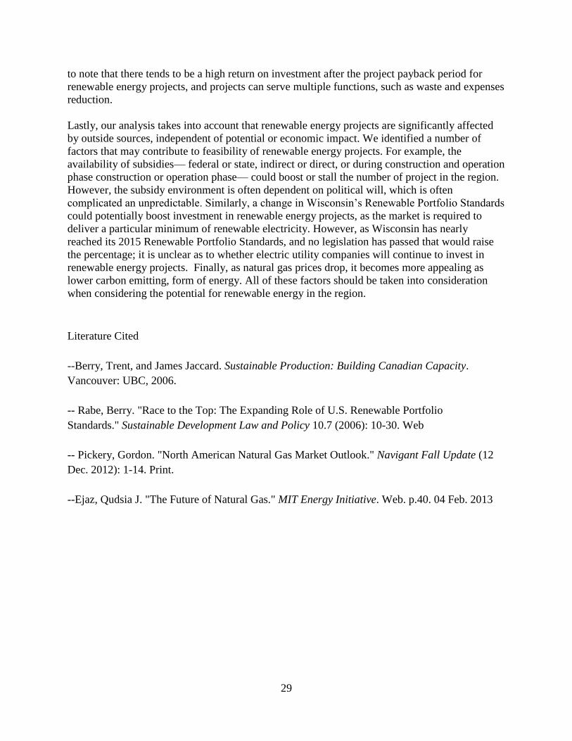
Herd InventoryAssumed Herd
Composition
Animal
Count
Typical
Animal
Mass (lbs)
Volatile
Solids
per lb
TAM/yr
Total Volatile
Solids/yr
Volatile
Solids %
Destruction
Cu ft Methane
Yield per lb
VS Destroyed
Methane Yield
cu ft/yr
Methane Yield
mm Btu/yr
Enter herd or flock inventory
reported by USDA in column C.
Beef CattleEnter %'s below
& total here ->171,400
Feedlot Steers and Heifers 33.33% 57,127.62 915.00 2.60 135,906,607.98 45% 5.29 323,525,680.30 313,819.91
Calves 33.33% 57,127.62 397.00 2.60 58,967,129.36 45% 2.72 72,175,766.34 70,010.49
Steers 0.00 794.00 2.60 - 45% 2.72 - -
Heifers 0.00 794.00 2.60 - 45% 2.72 - -
Cows 33.33% 57,127.62 1,102.00 2.60 163,682,056.82 45% 2.72 200,346,837.55 194,336.43
Bulls 0.00 1,587.00 2.60 - 45% 2.72 - -
99.99% 578,166.84
Dairy CattleEnter %'s below
& total here ->48,000
Calves 18.00% 8,640.00 397.00 2.60 8,918,208.00 35% 3.84 11,986,071.55 11,626.49
Heifers 18.00% 8,640.00 903.00 3.65 28,477,008.00 35% 3.84 38,273,098.75 37,124.91
Cows 64.00% 30,720.00 1,345.00 3.65 150,812,160.00 35% 3.84 202,691,543.04 196,610.80
100.00% 245,362.19
SwineEnter %'s below
& total here ->77,636
Market 92.00% 71,425.12 101.00 3.10 22,363,205.07 50% 7.53 84,197,467.10 81,671.54
Breeding 8.00% 6,210.88 399.00 3.10 7,682,237.47 50% 5.77 22,163,255.11 21,498.36
100.00% 103,169.90
PoultryEnter %'s below
& total here ->25,563
Layers 92.91% 23,750.58 3.50 4.40 365,758.98 60% 5.45 1,196,031.87 1,160.15
Broilers 6.82% 1,743.40 1.50 6.20 16,213.59 60% 4.81 46,792.42 45.39
Turkeys 0.27% 69.02 7.50 3.32 1,718.60 60% 4.81 4,959.88 4.81
100.00% 1,210.35
Sheep Enter total here -> 3,372 154.00 3.36 1,744,807.68 55% 5.77 5,537,147.17 5,371.03
Total Energy Potential MM Btu/yr 933,280.3115
Trillion Btu/yr 0.9333
3. Table 1.3: Estimated Annual Livestock Residue Potential
4. Table 1.4: Estimated Annual Logging Residue Potential
Column B C D E F G
Formula =B*C/D =E*F
Units cu ft/yr % harvested cu ft/cord cords/yr million Btu/cord million Btu/yr
Hardwood 4,350,080.0 33% 80 17,944.1 25 448,602.00
Softwood 473,984.0 33% 85 1,840.2 15 27,602.60
Total Energy Potential MM Btu/yr 476,204.5976
Trillion Btu/yr 0.4762
32
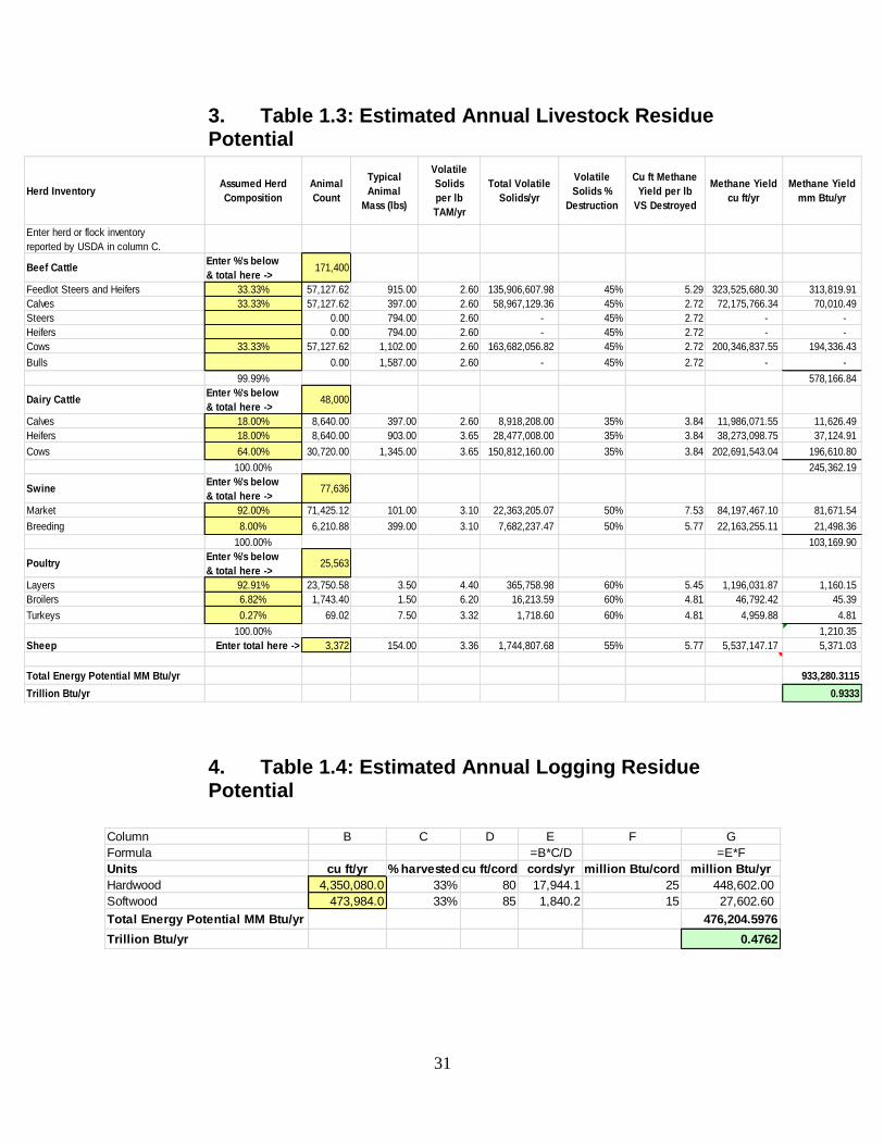
5. Table 1.5: Estimated Annual Wind Energy Potential
B. Green County
1. Table 2.1: Estimated Annual Renewable Energy Potential Summary
2. Table 2.2: Estimated Annual Crop Residue Potential
County Area in sq miles 1,148.0000 sq miles
Acres/sq mile 640 acres/sq mile
County Area in acres 734,720.00 acres =a*b
% Available for Wind Development 5.00%
Acres Available for Development 36,736.00 acres =A*B
Turbine Size 1.65 MW
Acres per Unit 40 acres
MW Installed per Acre 0.04125 MW/acre =D/E
Capacity Factor (%) 25.00%
Annual Hours 8,760 hours/year
MW hrs/yr 3,318,638.4000 =C*F*G*H
Trillion Btu/yr 11.3232 =I*3.412/10 6̂
Resource Energy Content Trillion Btu/yr
Agricultural Crop Residue 3.8834
Livestock Residue Methane 0.1958
Logging Residue -
Wind 5.7601
Total 9.8393

33
Herd InventoryAssumed Herd
CompositionAnimal Count
Typical Animal
Mass (lbs)
Volatile Solids
per lb TAM/yr
Total Volatile
Solids/yr
Volatile Solids
% Destruction
Cu ft Methane
Yield per lb
VS Destroyed
Methane Yield
cu ft/yr
Methane Yield
mm Btu/yr
Enter herd or flock inventory
reported by USDA in column C.
Beef CattleEnter %'s below
& total here ->5,294
Feedlot Steers and Heifers 33.33% 1,764.49 915.00 2.60 4,197,722.19 45% 5.29 9,992,677.66 9,692.90
Calves 33.33% 1,764.49 397.00 2.60 1,821,306.78 45% 2.72 2,229,279.50 2,162.40
Steers 0.00 794.00 2.60 - 45% 2.72 - -
Heifers 0.00 794.00 2.60 - 45% 2.72 - -
Cows 33.33% 1,764.49 1,102.00 2.60 5,055,617.32 45% 2.72 6,188,075.60 6,002.43
Bulls 0.00 1,587.00 2.60 - 45% 2.72 - -
99.99% 17,857.73
Dairy CattleEnter %'s below
& total here ->30,709
Calves 18.00% 5,527.64 397.00 2.60 5,705,626.25 35% 3.84 7,668,361.69 7,438.31
Heifers 18.00% 5,527.64 903.00 3.65 18,218,813.07 35% 3.84 24,486,084.77 23,751.50
Cows 64.00% 19,653.82 1,345.00 3.65 96,485,506.91 35% 3.84 129,676,521.29 125,786.23
100.00% 156,976.04
SwineEnter %'s below
& total here ->12,692
Market 88.84% 11,275.57 101.00 3.10 3,530,381.84 50% 7.53 13,291,887.64 12,893.13
Breeding 11.16% 1,416.43 399.00 3.10 1,751,978.80 50% 5.77 5,054,458.85 4,902.83
100.00% 17,795.96
PoultryEnter %'s below
& total here ->5,272
Layers 3.07% 161.85 3.50 4.40 2,492.50 60% 5.45 8,150.46 7.91
Broilers 40.31% 2,125.14 1.50 6.20 19,763.83 60% 4.81 57,038.42 55.33
Turkeys 56.62% 2,985.01 7.50 3.32 74,326.66 60% 4.81 214,506.74 208.07
100.00% 271.30
Sheep Enter total here -> 1,846 154.00 3.36 955,194.24 55% 5.77 3,031,308.92 2,940.37
Total Energy Potential MM Btu/yr 195,841.4010
Trillion Btu/yr 0.1958
3. Table 2.3: Estimated Annual Livestock Residue Potential
Crop Acres
HarvestedYield Units
Convert
to lbs
Removal
FractionMoisture %
Residue to
Crop Ratio
Annual Biomass
Potential (lbs)
Btu Content
per dry lbMillion Btu/yr
Barley (Barley All) 554.40 57.67 bu 48 0.75 14.5% 1.2 1,180,858.69 7,500 8,856.44
Canola lbs 1 0.75 8.0% 2.2 - 7,500 -
Corn for Stover (Corn For Grain) 85,522.50 154.04 bu 56 0.5 15.5% 1.0 311,694,140.39 7,768 2,421,240.08
Cotton lbs 1 0.75 12.0% 4.5 - 7,500 -
Dry Beans (Beans Dry Edible) lbs 1 0.75 13.0% 1.2 - 7,500 -
Flaxseed bu 1 0.75 8.0% 1.2 - 7,500 -
Oat Straw (Oats) 5,281.18 70.56 bu 32 0.75 14.0% 1.3 9,998,051.76 7,626 76,245.14
Peanuts lbs 1 0.75 9.9% 1.0 - 7,500 -
Peas (Green Peas for Processing) tons 2,000 0.75 9.8% 1.5 - 7,500 -
Potatoes 5.00 cwt 100 0.75 13.3% 0.4 - 7,500 -
Rice lbs 1 0.75 15.0% 1.4 - 7,500 -
Rye 77.50 bu 56 0.75 10.0% 1.6 - 7,500 -
Safflower lbs 1 0.75 8.0% 1.2 - 7,500 -
Sorghum bu 56 0.75 12.0% 1.4 - 7,500 -
Soybeans 44,990.17 44.79 bu 60 0.75 13.0% 2.1 165,672,232.89 7,500 1,242,541.75
Sugar Beets tons 2,000 0.75 62.8% 1.0 - 7,500 -
Sugar Cane tons 2,000 0.75 62.8% 1.6 - 7,500 -
Sunflower (Sunflower All) lbs 1 0.75 10.0% 2.1 - 7,500 -
Wheat Straw (Wheat All) 5,501.78 65.50 bu 60 0.75 13.5% 1.3 18,235,443.01 7,375 134,486.39
CRP and similar grassland 2.00 tons 2,000 0.75 20.0% 1.0 - 7,500 -
Brushland on 5 yr cycle 0.84 tons 2,000 0.75 20.0% 1.0 - 7,500 -
Total Energy Potential MM Btu/yr 3,883,369.8043
Trillion Btu/yr 3.8834

34
4. Table 2.4: Estimated Annual Wind Energy Potential
C. Iowa County
1. Table 3.1: Estimated Annual Renewable Energy Potential Summary
2. Table 3.2: Estimated Annual Crop Residue Potential
County Area in sq miles 583.99 sq miles
Acres/sq mile 640 acres/sq mile
County Area in acres 373,753.60 acres
% Available for Wind Development 5.00%
Acres Available for Development 18,687.68 acres
Turbine Size 1.65 MW
Acres per Unit 40 acres
MW Installed per Acre 0.04125 MW/acre
Capacity Factor (%) 25.00%
Annual Hours 8,760 hours/year
MW hrs/yr 1,688,198.2920
Trillion Btu/yr 5.7601
Resource Energy Content Trillion Btu/yr
Agricultural Crop Residue 2.6644
Livestock Residue Methane 0.4459
Logging Residue -
Wind 7.5216
Total 10.6319

35
Herd InventoryAssumed Herd
Composition
Animal
Count
Typical
Animal
Mass (lbs)
Volatile
Solids
per lb
TAM/yr
Total Volatile
Solids/yr
Volatile
Solids %
Destruction
Cu ft Methane
Yield per lb
VS Destroyed
Methane Yield
cu ft/yr
Methane Yield
mm Btu/yr
Enter herd or flock inventory
reported by USDA in column C.
Beef CattleEnter %'s below
& total here -> 87,000
Feedlot Steers and Heifers 33.33% 28,997.10 915.00 2.60 68,984,100.90 45% 5.29 164,216,652.19 159,290.15
Calves 33.33% 28,997.10 397.00 2.60 29,930,806.62 45% 2.72 36,635,307.30 35,536.25
Steers 0.00 794.00 2.60 - 45% 2.72 - -
Heifers 0.00 794.00 2.60 - 45% 2.72 - -
Cows 33.33% 28,997.10 1,102.00 2.60 83,082,490.92 45% 2.72 101,692,968.89 98,642.18
Bulls 0.00 1,587.00 2.60 - 45% 2.72 - -
99.99% 293,468.58
Dairy CattleEnter %'s below
& total here ->24,509
Calves 18.00% 4,411.64 397.00 2.60 4,553,691.05 35% 3.84 6,120,160.78 5,936.56
Heifers 18.00% 4,411.64 903.00 3.65 14,540,532.87 35% 3.84 19,542,476.18 18,956.20
Cows 64.00% 15,685.82 1,345.00 3.65 77,005,602.91 35% 3.84 103,495,530.31 100,390.66
100.00% 125,283.42
SwineEnter %'s below
& total here ->17,436
Market 91.00% 15,867.09 101.00 3.10 4,967,986.16 50% 7.53 18,704,467.91 18,143.33
Breeding 9.00% 1,569.27 399.00 3.10 1,941,033.44 50% 5.77 5,599,881.46 5,431.89
100.00% 23,575.22
PoultryEnter %'s below
& total here ->94,791
Layers 50.00% 47,395.45 3.50 4.40 729,890.00 60% 5.45 2,386,740.30 2,315.14
Broilers 50.00% 47,395.45 1.50 6.20 440,777.73 60% 4.81 1,272,084.52 1,233.92
Turkeys 0.00% 0.00 7.50 3.32 - 60% 4.81 - -
100.00% 3,549.06
Sheep Enter total here -> 0 154.00 3.36 - 55% 5.77 - -
Total Energy Potential MM Btu/yr 445,876.2817
Trillion Btu/yr 0.4459
3. Table 3.3: Estimated Annual Livestock Residue Potential
Crop Acres
HarvestedYield Units
Convert
to lbs
Removal
FractionMoisture %
Residue to
Crop Ratio
Annual Biomass
Potential (lbs)
Btu Content
per dry lbMillion Btu/yr
Barley (Barley All) 1,075.00 55.80 bu 48 0.75 14.5% 1.2 2,215,605.96 7,500 16,617.04
Canola 0.00 0.00 lbs 1 0.75 8.0% 2.2 - 7,500 -
Corn for Stover (Corn For Grain) 57,730.00 157.33 bu 56 0.5 15.5% 1.0 214,895,756.89 7,768 1,669,310.24
Cotton 0.00 0.00 lbs 1 0.75 12.0% 4.5 - 7,500 -
Dry Beans (Beans Dry Edible) 0.00 0.00 lbs 1 0.75 13.0% 1.2 - 7,500 -
Flaxseed 0.00 0.00 bu 1 0.75 8.0% 1.2 - 7,500 -
Oat Straw (Oats) 3,980.00 67.16 bu 32 0.75 14.0% 1.3 7,172,496.07 7,626 54,697.46
Peanuts 0.00 0.00 lbs 1 0.75 9.9% 1.0 - 7,500 -
Peas (Green Peas for Processing) 812.50 1.94 tons 2,000 0.75 9.8% 1.5 3,194,876.95 7,500 23,961.58
Potatoes 772.86 389.14 cwt 100 0.75 13.3% 0.4 7,822,555.27 7,500 58,669.16
Rice 0.00 0.00 lbs 1 0.75 15.0% 1.4 - 7,500 -
Rye 0.00 0.00 bu 56 0.75 10.0% 1.6 - 7,500 -
Safflower 0.00 0.00 lbs 1 0.75 8.0% 1.2 - 7,500 -
Sorghum 0.00 0.00 bu 56 0.75 12.0% 1.4 - 7,500 -
Soybeans 28,710.00 46.04 bu 60 0.75 13.0% 2.1 108,672,477.61 7,500 815,043.58
Sugar Beets 0.00 0.00 tons 2,000 0.75 62.8% 1.0 - 7,500 -
Sugar Cane 0.00 0.00 tons 2,000 0.75 62.8% 1.6 - 7,500 -
Sunflower (Sunflower All) 0.00 0.00 lbs 1 0.75 10.0% 2.1 - 7,500 -
Wheat Straw (Wheat All) 1,080.00 64.70 bu 60 0.75 13.5% 1.3 3,535,900.29 7,375 26,077.26
CRP and similar grassland 0.00 2.00 tons 2,000 0.75 20.0% 1.0 - 7,500 -
Brushland on 5 yr cycle 0.00 0.84 tons 2,000 0.75 20.0% 1.0 - 7,500 -
Total Energy Potential MM Btu/yr 2,664,376.3277
Trillion Btu/yr 2.6644
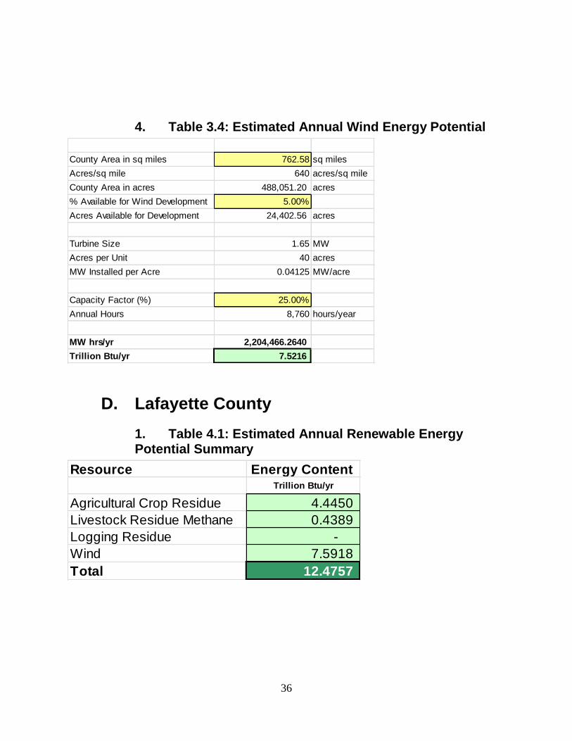
36
4. Table 3.4: Estimated Annual Wind Energy Potential
D. Lafayette County
1. Table 4.1: Estimated Annual Renewable Energy Potential Summary
County Area in sq miles 762.58 sq miles
Acres/sq mile 640 acres/sq mile
County Area in acres 488,051.20 acres
% Available for Wind Development 5.00%
Acres Available for Development 24,402.56 acres
Turbine Size 1.65 MW
Acres per Unit 40 acres
MW Installed per Acre 0.04125 MW/acre
Capacity Factor (%) 25.00%
Annual Hours 8,760 hours/year
MW hrs/yr 2,204,466.2640
Trillion Btu/yr 7.5216
Resource Energy Content Trillion Btu/yr
Agricultural Crop Residue 4.4450
Livestock Residue Methane 0.4389
Logging Residue -
Wind 7.5918
Total 12.4757

37
2. Table 4.2: Estimated Annual Crop Residue Potential
3. Table 4.3: Estimated Annual Livestock Residue Potential
Crop Acres
HarvestedYield Units
Convert
to lbs
Removal
FractionMoisture %
Residue to
Crop Ratio
Annual Biomass
Potential (lbs)
Btu Content
per dry lbMillion Btu/yr
Barley (Barley All) 0.00 0.00 bu 48 0.75 14.5% 1.2 - 7,500 -
Canola 0.00 0.00 lbs 1 0.75 8.0% 2.2 - 7,500 -
Corn for Stover (Corn For Grain) 105,558.00 150 bu 56 0.5 15.5% 1.0 374,625,342.00 7,768 2,910,089.66
Cotton 0.00 0.00 lbs 1 0.75 12.0% 4.5 - 7,500 -
Dry Beans (Beans Dry Edible) 0.00 0.00 lbs 1 0.75 13.0% 1.2 - 7,500 -
Flaxseed 0.00 0.00 bu 1 0.75 8.0% 1.2 - 7,500 -
Oat Straw (Oats) 4,013.00 67 bu 32 0.75 14.0% 1.3 7,214,346.67 7,626 55,016.61
Peanuts 0.00 0.00 lbs 1 0.75 9.9% 1.0 - 7,500 -
Peas (Green Peas for Processing) 0.00 0.00 tons 2,000 0.75 9.8% 1.5 - 7,500 -
Potatoes 0.00 0.00 cwt 100 0.75 13.3% 0.4 - 7,500 -
Rice 0.00 0.00 lbs 1 0.75 15.0% 1.4 - 7,500 -
Rye 0.00 0.00 bu 56 0.75 10.0% 1.6 - 7,500 -
Safflower 0.00 0.00 lbs 1 0.75 8.0% 1.2 - 7,500 -
Sorghum 0.00 0.00 bu 56 0.75 12.0% 1.4 - 7,500 -
Soybeans 50,633.00 47.40 bu 60 0.75 13.0% 2.1 197,316,345.30 7,500 1,479,872.59
Sugar Beets 0.00 0.00 tons 2,000 0.75 62.8% 1.0 - 7,500 -
Sugar Cane 0.00 0.00 tons 2,000 0.75 62.8% 1.6 - 7,500 -
Sunflower (Sunflower All) 0.00 0.00 lbs 1 0.75 10.0% 2.1 - 7,500 -
Wheat Straw (Wheat All) bu 60 0.75 13.5% 1.3 - 7,375 -
CRP and similar grassland 2.00 tons 2,000 0.75 20.0% 1.0 - 7,500 -
Brushland on 5 yr cycle 0.84 tons 2,000 0.75 20.0% 1.0 - 7,500 -
Total Energy Potential MM Btu/yr 4,444,978.8541
Trillion Btu/yr 4.4450
Herd InventoryAssumed Herd
Composition
Animal
Count
Typical
Animal
Mass (lbs)
Volatile
Solids
per lb
TAM/yr
Total Volatile
Solids/yr
Volatile
Solids %
Destruction
Cu ft Methane
Yield per lb
VS Destroyed
Methane Yield
cu ft/yr
Methane Yield
mm Btu/yr
Enter herd or flock inventory
reported by USDA in column C.
Beef CattleEnter %'s below
& total here ->68,838
Feedlot Steers and Heifers 33.33% 22,943.71 915.00 2.60 54,583,075.15 45% 5.29 129,935,010.39 126,036.96
Calves 33.33% 22,943.71 397.00 2.60 23,682,492.71 45% 2.72 28,987,371.08 28,117.75
Steers 0.00 794.00 2.60 - 45% 2.72 - -
Heifers 0.00 794.00 2.60 - 45% 2.72 - -
Cows 33.33% 22,943.71 1,102.00 2.60 65,738,304.71 45% 2.72 80,463,684.97 78,049.77
Bulls 0.00 1,587.00 2.60 - 45% 2.72 - -
99.99% 232,204.48
Dairy CattleEnter %'s below
& total here ->30,100
Calves 18.00% 5,418.00 397.00 2.60 5,592,459.60 35% 3.84 7,516,265.70 7,290.78
Heifers 18.00% 5,418.00 903.00 3.65 17,857,457.10 35% 3.84 24,000,422.34 23,280.41
Cows 64.00% 19,264.00 1,345.00 3.65 94,571,792.00 35% 3.84 127,104,488.45 123,291.35
100.00% 153,862.54
SwineEnter %'s below
& total here ->21,673
Market 50.00% 10,836.50 101.00 3.10 3,392,908.15 50% 7.53 12,774,299.18 12,391.07
Breeding 50.00% 10,836.50 399.00 3.10 13,403,666.85 50% 5.77 38,669,578.86 37,509.49
100.00% 49,900.56
PoultryEnter %'s below
& total here ->674
Layers 0.00 3.50 4.40 - 60% 5.45 - -
Broilers 0.00 1.50 6.20 - 60% 4.81 - -
Turkeys 0.00 7.50 3.32 - 60% 4.81 - -
0.00% -
Sheep Enter total here -> 1,812 154.00 3.36 937,601.28 55% 5.77 2,975,477.66 2,886.21
Total Energy Potential MM Btu/yr 438,853.8007
Trillion Btu/yr 0.4389

38
4. Table 4.4: Estimated Annual Wind Energy Potential
E. Richland County
1. Table 5.1: Estimated Annual Renewable Energy Potential Summary
County Area in sq miles 635.00 sq miles
Acres/sq mile 640 acres/sq mile
County Area in acres 406,400.00 acres
% Available for Wind Development 5.00%
Acres Available for Development 20,320.00 acres
Turbine Size 2 MW
Acres per Unit 40 acres
MW Installed per Acre 0.05 MW/acre
Capacity Factor (%) 25.00%
Annual Hours 8,760 hours/year
MW hrs/yr 2,225,040.0000
Trillion Btu/yr 7.5918
Resource Quantity Units Energy Content Trillion Btu/yr
Agricultural Crop Residue Tons 0.6591
Livestock Residue Methane SCF 0.1000
Logging Residue Tons 0.1340
Wind kW-hr 5.7814
Total 6.6745
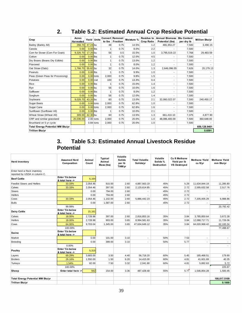
39
Herd InventoryAssumed Herd
Composition
Animal
Count
Typical
Animal
Mass (lbs)
Volatile
Solids
per lb
TAM/yr
Total Volatile
Solids/yr
Volatile
Solids %
Destruction
Cu ft Methane
Yield per lb
VS Destroyed
Methane Yield
cu ft/yr
Methane Yield
mm Btu/yr
Enter herd or flock inventory
reported by USDA in column C.
Beef CattleEnter %'s below
& total here ->6,164
Feedlot Steers and Heifers 33.33% 2,054.46 915.00 2.60 4,887,563.19 45% 5.29 11,634,844.19 11,285.80
Calves 33.33% 2,054.46 397.00 2.60 2,120,614.85 45% 2.72 2,595,632.58 2,517.76
Steers 0.00 794.00 2.60 - 45% 2.72 - -
Heifers 0.00 794.00 2.60 - 45% 2.72 - -
Cows 33.33% 2,054.46 1,102.00 2.60 5,886,442.23 45% 2.72 7,205,005.29 6,988.86
Bulls 0.00 1,587.00 2.60 - 45% 2.72 - -
99.99% 20,792.42
Dairy CattleEnter %'s below
& total here ->15,161
Calves 18.00% 2,728.98 397.00 2.60 2,816,853.16 35% 3.84 3,785,850.64 3,672.28
Heifers 18.00% 2,728.98 903.00 3.65 8,994,581.63 35% 3.84 12,088,717.71 11,726.06
Cows 64.00% 9,703.04 1,345.00 3.65 47,634,649.12 35% 3.84 64,020,968.42 62,100.34
100.00% 77,498.67
SwineEnter %'s below
& total here ->
Market 0.00 101.00 3.10 - 50% 7.53 - -
Breeding 0.00 399.00 3.10 - 50% 5.77 - -
0.00% -
PoultryEnter %'s below
& total here ->5,315
Layers 69.29% 3,683.00 3.50 4.40 56,718.20 60% 5.45 185,468.51 179.90
Broilers 29.16% 1,550.00 1.50 6.20 14,415.00 60% 4.81 41,601.69 40.35
Turkeys 1.54% 82.00 7.50 3.32 2,041.80 60% 4.81 5,892.63 5.72
100.00% 225.97
Sheep Enter total here -> 942 154.00 3.36 487,428.48 55% 5.77 1,546,854.28 1,500.45
Total Energy Potential MM Btu/yr 100,017.5109
Trillion Btu/yr 0.1000
2. Table 5.2: Estimated Annual Crop Residue Potential
3. Table 5.3: Estimated Annual Livestock Residue Potential
Crop Acres
HarvestedYield Units
Convert
to lbs
Removal
FractionMoisture %
Residue to
Crop Ratio
Annual Biomass
Potential (lbs)
Btu Content
per dry lbMillion Btu/yr
Barley (Barley All) 266.70 47.24 bu 48 0.75 14.5% 1.2 465,353.27 7,500 3,490.15
Canola 0.00 0.00 lbs 1 0.75 8.0% 2.2 - 7,500 -
Corn for Stover (Corn For Grain) 9,326.70 17.20 bu 56 0.5 15.5% 1.0 3,795,519.22 7,768 29,483.59
Cotton 0.00 0.00 lbs 1 0.75 12.0% 4.5 - 7,500 -
Dry Beans (Beans Dry Edible) 0.00 0.00 lbs 1 0.75 13.0% 1.2 - 7,500 -
Flaxseed 0.00 0.00 bu 1 0.75 8.0% 1.2 - 7,500 -
Oat Straw (Oats) 1,766.70 55.82 bu 32 0.75 14.0% 1.3 2,646,096.55 7,626 20,179.13
Peanuts 0.00 0.00 lbs 1 0.75 9.9% 1.0 - 7,500 -
Peas (Green Peas for Processing) 0.00 0.00 tons 2,000 0.75 9.8% 1.5 - 7,500 -
Potatoes 0.00 0.00 cwt 100 0.75 13.3% 0.4 - 7,500 -
Rice 0.00 0.00 lbs 1 0.75 15.0% 1.4 - 7,500 -
Rye 0.00 0.00 bu 56 0.75 10.0% 1.6 - 7,500 -
Safflower 0.00 0.00 lbs 1 0.75 8.0% 1.2 - 7,500 -
Sorghum 0.00 0.00 bu 56 0.75 12.0% 1.4 - 7,500 -
Soybeans 9,026.70 43.20 bu 60 0.75 13.0% 2.1 32,060,022.07 7,500 240,450.17
Sugar Beets 0.00 0.00 tons 2,000 0.75 62.8% 1.0 - 7,500 -
Sugar Cane 0.00 0.00 tons 2,000 0.75 62.8% 1.6 - 7,500 -
Sunflower (Sunflower All) 0.00 0.00 lbs 1 0.75 10.0% 2.1 - 7,500 -
Wheat Straw (Wheat All) 309.00 42.30 bu 60 0.75 13.5% 1.3 661,410.10 7,375 4,877.90
CRP and similar grassland 20,036.00 2.00 tons 2,000 0.75 20.0% 1.0 48,086,400.00 7,500 360,648.00
Brushland on 5 yr cycle 0.84 tons 2,000 0.75 20.0% 1.0 - 7,500 -
Total Energy Potential MM Btu/yr 659,128.9401
Trillion Btu/yr 0.6591

40
4. Table 5.4: Estimated Annual Logging Residue Potential
5. Table 5.5: Estimated Annual Wind Energy Potential
Units cu ft/yr % harvested cu ft/cord cords/yr million Btu/cord million Btu/yr
Hardwood 1,155,740.8 33% 80 4,767.4 25 119,185.77
Softwood 253,699.2 33% 85 984.9 15 14,774.25
Total Energy Potential MM Btu/yr 133,960.0175
Trillion Btu/yr 0.1340
County Area in sq miles 586.15 sq miles
Acres/sq mile 640 acres/sq mile
County Area in acres 375,136.00 acres
% Available for Wind Development 5.00%
Acres Available for Development 18,756.80 acres
Turbine Size 1.65 MW
Acres per Unit 40 acres
MW Installed per Acre 0.04125 MW/acre
Capacity Factor (%) 25.00%
Annual Hours 8,760 hours/year
MW hrs/yr 1,694,442.4200
Trillion Btu/yr 5.7814
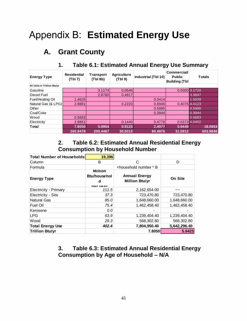
41
Estimated Energy Use
A. Grant County
1. Table 6.1: Estimated Annual Energy Use Summary
2. Table 6.2: Estimated Annual Residential Energy Consumption by Household Number
3. Table 6.3: Estimated Annual Residential Energy Consumption by Age of Household – N/A
Energy TypeResidential
(Tbl 7)
Transport
(Tbl 8b)
Agriculture
(Tbl 9)Industrial (Tbl 10)
Commercial/
Public
Building (Tbl
Totals
All Units in Trillion Btu/yr
Gasoline 3.1174 0.0546 0.0000 3.1720
Diesel Fuel 2.8780 0.4917 3.3697
Fuel/Heating Oil 1.4625 0.0414 1.5039
Natural Gas (& LPG) 2.8881 0.2220 0.8946 0.4076 4.4123
Other 0.5995 0.5995
Coal/Coke 0.3944 0.3944
Wood 0.5683 0.5683
Electricity 2.8861 0.1440 0.4778 0.5373 4.0452
Total 7.8050 5.9954 0.9123 2.4077 0.9449 18.0653
260.9478 200.4467 30.5013 80.4976 31.5912 603.9846
Total Number of Households 19,396
Column B C D
Formula =household number * B
Energy Type
Million
Btu/househol
d
per year
Annual Energy
Million Btu/yrOn Site
Electricity - Primary 111.5 2,162,654.00 −−
Electricity - Site 37.3 723,470.80 723,470.80
Natural Gas 85.0 1,648,660.00 1,648,660.00
Fuel Oil 75.4 1,462,458.40 1,462,458.40
Kerosene 0.0 - -
LPG 63.9 1,239,404.40 1,239,404.40
Wood 29.3 568,302.80 568,302.80
Total Energy Use 402.4 7,804,950.40 5,642,296.40
Trillion Btu/yr 7.8050 5.6423

42
4. Table 6.4: Estimated Annual Fuel Consumption Based on VMT
5. Table 6.5: Estimated Annual Fuel Consumption Based on Vehicle Registration
Total Annual VMT in County 619092119.5
Formula =B*Total VMT =C/D
Composition of VMT % of VMT Miles Traveled MPG Annual Fuel Use
Passenger Cars 55.8% 345,453,402.68 22.4 15,422,026.91
Light Trucks/SUV 36.1% 223,492,255.14 18.0 12,416,236.40
Single Unit Trucks 2.7% 16,715,487.23 8.2 2,038,474.05
Combination Trucks 4.7% 29,097,329.62 5.1 5,705,358.75
Total Energy Use 99.3% 614,758,474.66 35,582,096.10
Formula =B*C =D/10 1̂2
Convert Fuel Use to Btu's Gallons/yr LHV Btu/gallon Btu/yr Trillion Btu/yr
Gasoline (Cars & Light Trucks/SUVs) 27,838,263.30 116,090 3,231,743,986,733.9000 3.2317
Diesel (Trucks) 7,743,832.80 129,060 999,419,061,212.5940 0.9994
CarsLight
Trucks
Heavy
Trucks
20114 25670 5186
Annual Fuel Use per Vehicle 554 612 4300 gallons
Btu/gallon LHV at 60F 116090 116090 129060 Btu/gallon
Total Energy Use 1,293,608.98 1,823,778.54 2,878,012.19 Million Btu/yr
Trillion Btu/year 3.1174 2.8780

43
Barley - All 983.00 7.24 0.89 0.82 29.88 acre 7,116.92 874.87 806.06 29,372.04
Beans - Dry Edible 7.43 0.91 0.75 27.50 acre - - - -
Canola 4.50 0.75 0.00 26.80 acre - - - -
Corn for Grain 154,000.00 9.37 1.15 9.58 35.63 acre 1,442,980.00 177,100.00 1,475,320.00 5,487,020.00
Corn for Silage (Corn) 9.37 1.15 9.58 35.63 acre - - - -
Flaxseed 7.24 0.89 0.82 29.88 acre - - - -
Hay Alfalfa - Dry (Alfalfa) 9.80 0.81 0.00 32.73 acre - - - -
Hay - All (Alfalfa) 132,220.00 9.80 0.81 0.00 32.73 acre 1,295,756.00 107,098.20 - 4,327,560.60
Hay Other - Dry (Alfalfa) 9.80 0.81 0.00 32.73 acre - - - -
Oats 17,390.00 7.24 0.89 0.82 29.88 acre 125,903.60 15,477.10 14,259.80 519,613.20
Peas for Processing - Green 5.19 0.64 0.35 12.75 acre - - - -
Potatoes - Dry Land 24.18 2.00 0.00 205.27 acre - - - -
Potatoes - Irrigated 48.89 2.00 0.00 319.22 acre - - - -
Rye 7.24 0.89 0.82 29.88 acre - - - -
Soybeans 52,730.00 7.43 0.91 0.75 27.50 acre 391,783.90 47,984.30 39,547.50 1,450,075.00
Sugarbeets 28.92 3.54 2.76 100.75 acre - - - -
Sunflower - All 5.70 1.00 2.00 30.72 acre - - - -
Sunflower Seed for Oil 5.70 1.00 2.00 30.72 acre - - - -
Sunflower Seed Non-Oil Uses 5.70 1.00 2.00 30.72 acre - - - -
Sweet Corn for Processing 7.99 0.98 0.49 18.00 acre - - - -
Wheat - All 1,183.00 7.24 0.89 0.82 29.88 acre 8,564.92 1,052.87 970.06 35,348.04
Wheat Durum 7.24 0.89 0.82 29.88 acre - - - -
Wheat - Other Spring 7.24 0.89 0.82 29.88 acre - - - -
Winter Wheat - All 7.24 0.89 0.82 29.88 acre - - - -
Head Count
Dairy 48,000.00 0.13 0.02 0.11 4.00 cwt 936,000.00 144,000.00 792,000.00 28,800,000.00
Swine Farrow 6,588.00 9.05 1.11 4.06 148.25 litter 119,242.80 14,625.36 53,494.56 1,953,342.00
Swine Finish 71,049.00 0.91 0.11 0.34 12.38hea
d129,309.18 15,630.78 48,313.32 1,759,173.24
Beef Cow-Calf 114,256.00 6.07 0.74 1.62 59.25hea
d693,533.92 84,549.44 185,094.72 6,769,668.00
Beef Cattle (Finishing) 57,128.00 3.78 0.46 1.08 39.38hea
d215,943.84 26,278.88 61,698.24 2,249,700.64
Turkey 68.00 0.09 0.01 0.50 1.24hea
d6.12 0.68 34.00 84.32
Total Energy Use 5,366,141.20 634,672.48 2,671,538.26 53,380,957.08
Conversion Factor Btu/unit 129,090 116,090 91,547 3412
Trillion Btu/yr 0.6927 0.0737 0.2446 0.1821
LP Gas
gallons
Electric
kW-hr
Energy Input/Unit Annual Energy Use
CommodityAcres
Planted
Diesel
gallons
Gasolin
e
LP Gas
gallons
Electric
kW-hrUnit
Diesel
gallons
Gasoline
gallons
6. Table 6.6: Estimated Annual On Farm Energy Use
7. Table 6.7: Estimated Annual Industrial Energy Use
Manufacturing shipments ($1000) - Grant County,
(American FactFinder2, QuickFacts & 2007 2390
Total energy use per $ of GDP - State of MN, 2000 8700 1007.4
Energy budget (trillion Btu) 0.0000 2.4077
Energy Type TotalNet
Electricity
Residual
Fuel Oil
Distillate
Fuel Oil
Natural
Gas
LPG &
NGLCoal
Coke &
BreezeOther
Energy use in Trillion Btu - Midwest Census Region
(Table 1.2)4707 934 45 36 1619 130 554 217 1172
Energy use in % 100.00% 19.8428% 0.9560% 0.7648% 34.3956% 2.7618% 11.7697% 4.6102% 24.8991%
Energy Use Trillion Btu/yr (Total from Ex. 1) 0.0000 0.0000 0.0000 0.0000 0.0000 0.0000 0.0000 0.0000 0.0000
Energy Type TotalNet
Electricity
Residual
Fuel Oil
Distillate
Fuel Oil
Natural
Gas
LPG &
NGLCoal
Coke &
BreezeOther
Energy use in Trillion Btu - Midwest Census Region
(Table 1.2)4707 934 45 36 1619 130 554 217 1172
Energy use in % 100.00% 19.8428% 0.9560% 0.7648% 34.3956% 2.7618% 11.7697% 4.6102% 24.8991%
Energy Use Trillion Btu/yr (Total from Ex. 2) 2.4077 0.4778 0.0230 0.0184 0.8281 0.0665 0.2834 0.1110 0.5995
Energy consumption per Employee (million Btu) -
Midwest Census Region (Table 6.2)
Energy budget (trillion Btu)
Ex. 3a Composition of Industrial Energy Use - Manufacturing Shipments (County Level)
Ex. 3b Composition of Industrial Energy Use - Manufacturing Employees (County Level)
Ex. 1 Manufacturing Shipments Method (County Level) Ex. 2 Manufacturing Employees Method (County Level)
Manufacturing employees - Grant County (American
FactFinder2, 2007 Economic Census)
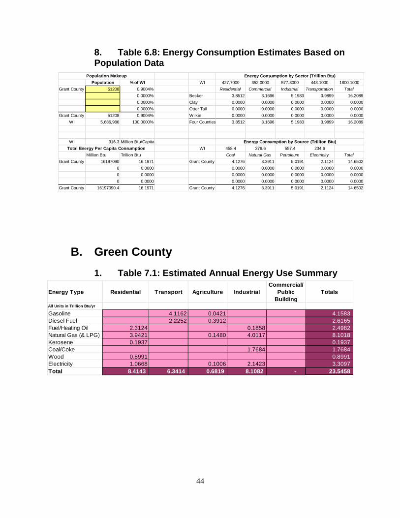
44
Population % of WI WI 427.7000 352.0000 577.3000 443.1000 1800.1000
Grant County 51208 0.9004% Residential Commercial Industrial Transportation Total
0.0000% Becker 3.8512 3.1696 5.1983 3.9899 16.2089
0.0000% Clay 0.0000 0.0000 0.0000 0.0000 0.0000
0.0000% Otter Tail 0.0000 0.0000 0.0000 0.0000 0.0000
Grant County 51208 0.9004% Wilkin 0.0000 0.0000 0.0000 0.0000 0.0000
WI 5,686,986 100.0000% Four Counties 3.8512 3.1696 5.1983 3.9899 16.2089
WI 316.3 Million Btu/Capita
WI 458.4 376.6 557.4 234.6
Million Btu Trillion Btu Coal Natural Gas Petroleum Electricity Total
Grant County 16197090 16.1971 Grant County 4.1276 3.3911 5.0191 2.1124 14.6502
0 0.0000 0.0000 0.0000 0.0000 0.0000 0.0000
0 0.0000 0.0000 0.0000 0.0000 0.0000 0.0000
0 0.0000 0.0000 0.0000 0.0000 0.0000 0.0000
Grant County 16197090.4 16.1971 Grant County 4.1276 3.3911 5.0191 2.1124 14.6502
Energy Consumption by Source (Trillion Btu)
Total Energy Per Capita Consumption
Population Makeup Energy Consumption by Sector (Trillion Btu)
8. Table 6.8: Energy Consumption Estimates Based on Population Data
B. Green County
1. Table 7.1: Estimated Annual Energy Use Summary
Energy Type Residential Transport Agriculture Industrial
Commercial/
Public
Building
Totals
All Units in Trillion Btu/yr
Gasoline 4.1162 0.0421 4.1583
Diesel Fuel 2.2252 0.3912 2.6165
Fuel/Heating Oil 2.3124 0.1858 2.4982
Natural Gas (& LPG) 3.9421 0.1480 4.0117 8.1018
Kerosene 0.1937 0.1937
Coal/Coke 1.7684 1.7684
Wood 0.8991 0.8991
Electricity 1.0668 0.1006 2.1423 3.3097
Total 8.4143 6.3414 0.6819 8.1082 - 23.5458
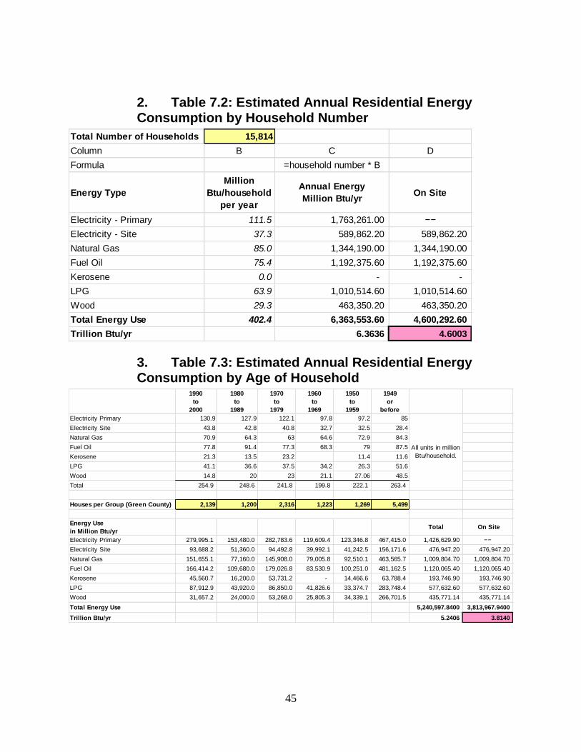
45
2. Table 7.2: Estimated Annual Residential Energy Consumption by Household Number
3. Table 7.3: Estimated Annual Residential Energy Consumption by Age of Household
Total Number of Households 15,814
Column B C D
Formula =household number * B
Energy Type
Million
Btu/household
per year
Annual Energy
Million Btu/yrOn Site
Electricity - Primary 111.5 1,763,261.00 −−
Electricity - Site 37.3 589,862.20 589,862.20
Natural Gas 85.0 1,344,190.00 1,344,190.00
Fuel Oil 75.4 1,192,375.60 1,192,375.60
Kerosene 0.0 - -
LPG 63.9 1,010,514.60 1,010,514.60
Wood 29.3 463,350.20 463,350.20
Total Energy Use 402.4 6,363,553.60 4,600,292.60
Trillion Btu/yr 6.3636 4.6003
1990
to
2000
1980
to
1989
1970
to
1979
1960
to
1969
1950
to
1959
1949
or
before
Electricity Primary 130.9 127.9 122.1 97.8 97.2 85
Electricity Site 43.8 42.8 40.8 32.7 32.5 28.4
Natural Gas 70.9 64.3 63 64.6 72.9 84.3
Fuel Oil 77.8 91.4 77.3 68.3 79 87.5
Kerosene 21.3 13.5 23.2 11.4 11.6
LPG 41.1 36.6 37.5 34.2 26.3 51.6
Wood 14.8 20 23 21.1 27.06 48.5
Total 254.9 248.6 241.8 199.8 222.1 263.4
Houses per Group (Green County) 2,139 1,200 2,316 1,223 1,269 5,499
Energy Use
in Million Btu/yrTotal On Site
Electricity Primary 279,995.1 153,480.0 282,783.6 119,609.4 123,346.8 467,415.0 1,426,629.90 −−
Electricity Site 93,688.2 51,360.0 94,492.8 39,992.1 41,242.5 156,171.6 476,947.20 476,947.20
Natural Gas 151,655.1 77,160.0 145,908.0 79,005.8 92,510.1 463,565.7 1,009,804.70 1,009,804.70
Fuel Oil 166,414.2 109,680.0 179,026.8 83,530.9 100,251.0 481,162.5 1,120,065.40 1,120,065.40
Kerosene 45,560.7 16,200.0 53,731.2 - 14,466.6 63,788.4 193,746.90 193,746.90
LPG 87,912.9 43,920.0 86,850.0 41,826.6 33,374.7 283,748.4 577,632.60 577,632.60
Wood 31,657.2 24,000.0 53,268.0 25,805.3 34,339.1 266,701.5 435,771.14 435,771.14
Total Energy Use 5,240,597.8400 3,813,967.9400
Trillion Btu/yr 5.2406 3.8140
All units in million
Btu/household.

46
4. Table 7.4: Estimated Annual Fuel Consumption Based on VMT
5. Table 7.5: Estimated Annual Fuel Consumption Based on Vehicle Registration
Total Annual VMT in Green County (2011) 328,209,095
Formula =B*Total VMT =C/D
Composition of VMT % of VMT Miles Traveled MPG Annual Fuel Use
Passenger Cars 55.8% 183,140,675.01 22.4 8,175,922.99
Light Trucks/SUV 36.1% 118,483,483.30 18.0 6,582,415.74
Single Unit Trucks 2.7% 8,861,645.57 8.2 1,080,688.48
Combination Trucks 4.7% 15,425,827.47 5.1 3,024,672.05
Total Energy Use 99.3% 325,911,631.34 18,863,699.27
Formula =B*C =D/10 1̂2
Convert Fuel Use to Btu's Gallons/yr LHV Btu/gallon Btu/yr Trillion Btu/yr
Gasoline (Cars & Light Trucks/SUVs) 14,758,338.73 116,090 1,713,295,543,180.6700 1.7133
Diesel (Trucks) 4,105,360.54 129,060 529,837,830,711.2910 0.5298
2010 Green County CarsLight
Trucks
Heavy
Trucks
15,715 19,595 3,055
Annual Fuel Use per Vehicle 554 612 4300 gallons
Btu/gallon LHV at 60F 116090 116090 129060 Btu/gallon
Total Energy Use 1,010,692.31 1,392,167.53 1,695,396.69 Million Btu/yr
Trillion Btu/year 2.4029 1.6954
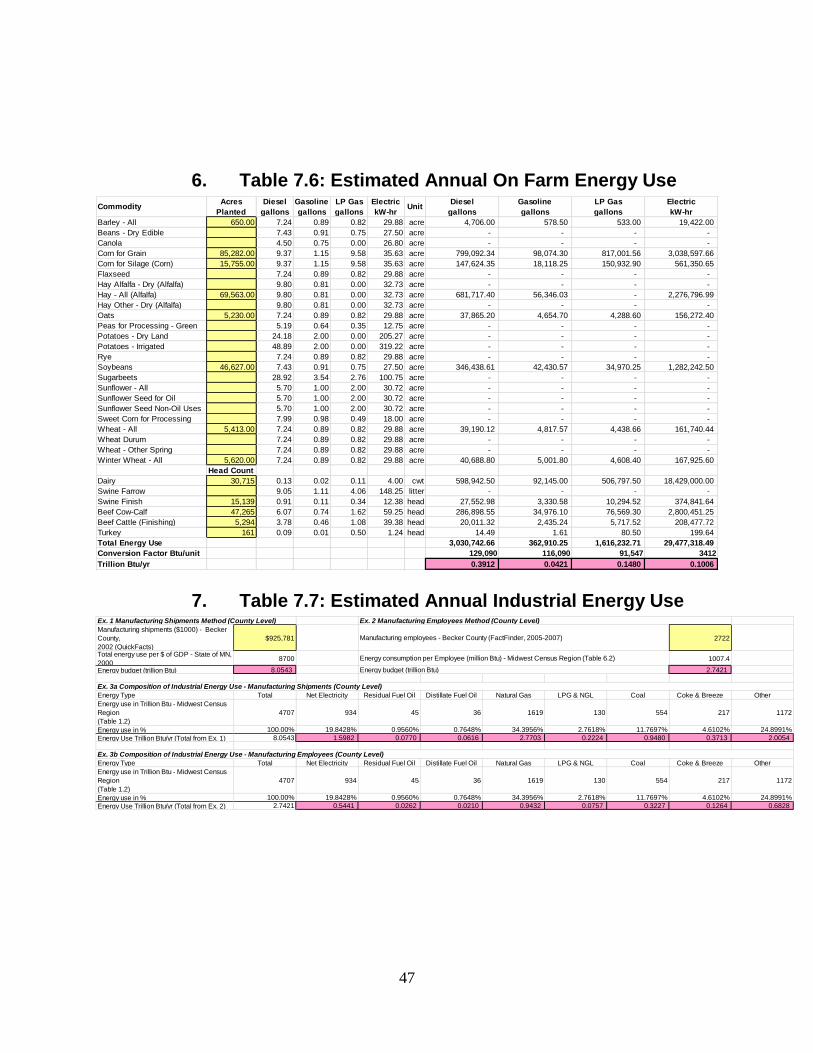
47
6. Table 7.6: Estimated Annual On Farm Energy Use
7. Table 7.7: Estimated Annual Industrial Energy Use
Barley - All 650.00 7.24 0.89 0.82 29.88 acre 4,706.00 578.50 533.00 19,422.00
Beans - Dry Edible 7.43 0.91 0.75 27.50 acre - - - -
Canola 4.50 0.75 0.00 26.80 acre - - - -
Corn for Grain 85,282.00 9.37 1.15 9.58 35.63 acre 799,092.34 98,074.30 817,001.56 3,038,597.66
Corn for Silage (Corn) 15,755.00 9.37 1.15 9.58 35.63 acre 147,624.35 18,118.25 150,932.90 561,350.65
Flaxseed 7.24 0.89 0.82 29.88 acre - - - -
Hay Alfalfa - Dry (Alfalfa) 9.80 0.81 0.00 32.73 acre - - - -
Hay - All (Alfalfa) 69,563.00 9.80 0.81 0.00 32.73 acre 681,717.40 56,346.03 - 2,276,796.99
Hay Other - Dry (Alfalfa) 9.80 0.81 0.00 32.73 acre - - - -
Oats 5,230.00 7.24 0.89 0.82 29.88 acre 37,865.20 4,654.70 4,288.60 156,272.40
Peas for Processing - Green 5.19 0.64 0.35 12.75 acre - - - -
Potatoes - Dry Land 24.18 2.00 0.00 205.27 acre - - - -
Potatoes - Irrigated 48.89 2.00 0.00 319.22 acre - - - -
Rye 7.24 0.89 0.82 29.88 acre - - - -
Soybeans 46,627.00 7.43 0.91 0.75 27.50 acre 346,438.61 42,430.57 34,970.25 1,282,242.50
Sugarbeets 28.92 3.54 2.76 100.75 acre - - - -
Sunflower - All 5.70 1.00 2.00 30.72 acre - - - -
Sunflower Seed for Oil 5.70 1.00 2.00 30.72 acre - - - -
Sunflower Seed Non-Oil Uses 5.70 1.00 2.00 30.72 acre - - - -
Sweet Corn for Processing 7.99 0.98 0.49 18.00 acre - - - -
Wheat - All 5,413.00 7.24 0.89 0.82 29.88 acre 39,190.12 4,817.57 4,438.66 161,740.44
Wheat Durum 7.24 0.89 0.82 29.88 acre - - - -
Wheat - Other Spring 7.24 0.89 0.82 29.88 acre - - - -
Winter Wheat - All 5,620.00 7.24 0.89 0.82 29.88 acre 40,688.80 5,001.80 4,608.40 167,925.60
Head Count
Dairy 30,715 0.13 0.02 0.11 4.00 cwt 598,942.50 92,145.00 506,797.50 18,429,000.00
Swine Farrow 9.05 1.11 4.06 148.25 litter - - - -
Swine Finish 15,139 0.91 0.11 0.34 12.38 head 27,552.98 3,330.58 10,294.52 374,841.64
Beef Cow-Calf 47,265 6.07 0.74 1.62 59.25 head 286,898.55 34,976.10 76,569.30 2,800,451.25
Beef Cattle (Finishing) 5,294 3.78 0.46 1.08 39.38 head 20,011.32 2,435.24 5,717.52 208,477.72
Turkey 161 0.09 0.01 0.50 1.24 head 14.49 1.61 80.50 199.64
Total Energy Use 3,030,742.66 362,910.25 1,616,232.71 29,477,318.49
Conversion Factor Btu/unit 129,090 116,090 91,547 3412
Trillion Btu/yr 0.3912 0.0421 0.1480 0.1006
CommodityDiesel
gallons
Acres
Planted
Gasoline
gallons
LP Gas
gallons
LP Gas
gallons
Electric
kW-hr
Electric
kW-hrUnit
Diesel
gallons
Gasoline
gallons
Manufacturing shipments ($1000) - Becker
County,
2002 (QuickFacts)
$925,781 2722
Total energy use per $ of GDP - State of MN,
20008700 1007.4
Energy budget (trillion Btu) 8.0543 2.7421
Energy Type Total Net Electricity Residual Fuel Oil Distillate Fuel Oil Natural Gas LPG & NGL Coal Coke & Breeze Other
Energy use in Trillion Btu - Midwest Census
Region
(Table 1.2)
4707 934 45 36 1619 130 554 217 1172
Energy use in % 100.00% 19.8428% 0.9560% 0.7648% 34.3956% 2.7618% 11.7697% 4.6102% 24.8991%
Energy Use Trillion Btu/yr (Total from Ex. 1) 8.0543 1.5982 0.0770 0.0616 2.7703 0.2224 0.9480 0.3713 2.0054
Energy Type Total Net Electricity Residual Fuel Oil Distillate Fuel Oil Natural Gas LPG & NGL Coal Coke & Breeze Other
Energy use in Trillion Btu - Midwest Census
Region
(Table 1.2)
4707 934 45 36 1619 130 554 217 1172
Energy use in % 100.00% 19.8428% 0.9560% 0.7648% 34.3956% 2.7618% 11.7697% 4.6102% 24.8991%
Energy Use Trillion Btu/yr (Total from Ex. 2) 2.7421 0.5441 0.0262 0.0210 0.9432 0.0757 0.3227 0.1264 0.6828
Ex. 1 Manufacturing Shipments Method (County Level)
Ex. 3a Composition of Industrial Energy Use - Manufacturing Shipments (County Level)
Ex. 2 Manufacturing Employees Method (County Level)
Manufacturing employees - Becker County (FactFinder, 2005-2007)
Energy consumption per Employee (million Btu) - Midwest Census Region (Table 6.2)
Energy budget (trillion Btu)
Ex. 3b Composition of Industrial Energy Use - Manufacturing Employees (County Level)
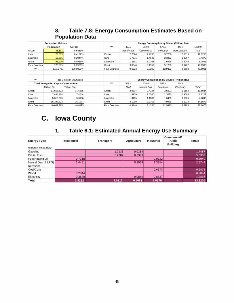
48
8. Table 7.8: Energy Consumption Estimates Based on Population Data
C. Iowa County
1. Table 8.1: Estimated Annual Energy Use Summary
Population % of WI WI 427.7 352.0 577.3 443.1 1800.0
Green 36,891 0.6459% Residential Commercial Industrial Transportation Total
Iowa 23,599 0.4132% Green 2.7624 2.2735 3.7286 2.8619 11.6258
Lafayette 16,815 0.2944% Iowa 1.7671 1.4543 2.3852 1.8307 7.4370
Grant 51,210 0.8966% Lafayette 1.2591 1.0363 1.6995 1.3045 5.2991
Four Counties 128,515 2.2500% Grant 3.8346 3.1559 5.1759 3.9727 16.1383
WI 5,711,767 100.0000% Four Counties 9.6233 7.9200 12.9893 9.9698 40.5001
WI 316.3 Million Btu/Capita
WI 458.4 376.6 557.4 234.6
Million Btu Trillion Btu Coal Natural Gas Petroleum Electricity Total
Green 11,668,623 11.6686 Green 2.9607 2.4324 3.6001 1.5152 10.5084
Iowa 7,464,364 7.4644 Iowa 1.8939 1.5560 2.3030 0.9693 6.7222
Lafayette 5,318,585 5.3186 Lafayette 1.3495 1.1087 1.6409 0.6906 4.7898
Grant 16,197,723 16.1977 Grant 4.1099 3.3765 4.9975 2.1034 14.5872
Four Counties 40,649,295 40.6493 Four Counties 10.3140 8.4735 12.5415 5.2785 36.6076
Total Energy Per Capita Consumption
Population Makeup Energy Consumption by Sector (Trillion Btu)
Energy Consumption by Source (Trillion Btu)
Energy Type Residential Transport Agriculture Industrial
Commercial/
Public
Building
Totals
All Units in Trillion Btu/yr
Gasoline 1.7133 0.0354 1.7487
Diesel Fuel 5.2984 0.3399 5.6383
Fuel/Heating Oil 0.7318 0.0722 0.8040
Natural Gas (& LPG) 1.4451 0.1039 1.3254 2.8744
Kerosene -
Coal/Coke 0.6873 0.6873
Wood 0.2844 0.2844
Electricity 0.3620 0.0889 0.8327 1.2836
Total 2.8232 7.0117 0.5681 2.9176 - 13.3205

49
2. Table 8.2: Estimated Annual Residential Energy Consumption by Household Number
3. Table 8.3: Estimated Annual Residential Energy Consumption by Age of Household
4. Table 8.4: Estimated Annual Fuel Consumption Based on VMT
Total Number of Households 9,705
Column B C D
Formula =household number * B
Energy Type
Million
Btu/household
per year
Annual Energy
Million Btu/yrOn Site
Electricity - Primary 111.5 1,082,107.50 −−
Electricity - Site 37.3 361,996.50 361,996.50
Natural Gas 85.0 824,925.00 824,925.00
Fuel Oil 75.4 731,757.00 731,757.00
Kerosene 0.0 - -
LPG 63.9 620,149.50 620,149.50
Wood 29.3 284,356.50 284,356.50
Total Energy Use 402.4 3,905,292.00 2,823,184.50
Trillion Btu/yr 3.9053 2.8232
1990
to
2000
1980
to
1989
1970
to
1979
1960
to
1969
1950
to
1959
1949
or
before
Electricity Primary 130.9 127.9 122.1 97.8 97.2 85
Electricity Site 43.8 42.8 40.8 32.7 32.5 28.4
Natural Gas 70.9 64.3 63 64.6 72.9 84.3
Fuel Oil 77.8 91.4 77.3 68.3 79 87.5
Kerosene 21.3 13.5 23.2 11.4 11.6
LPG 41.1 36.6 37.5 34.2 26.3 51.6
Wood 14.8 20 23 21.1 27.06 48.5
Total 254.9 248.6 241.8 199.8 222.1 263.4
Houses per Group 1,829 1,074 1,278 795 591 3,829
Energy Use
in Million Btu/yrTotal On Site
Electricity Primary 239,416.1 137,364.6 156,043.8 77,751.0 57,445.2 325,465.0 993,485.70 −−
Electricity Site 80,110.2 45,967.2 52,142.4 25,996.5 19,207.5 108,743.6 332,167.40 332,167.40
Natural Gas 129,676.1 69,058.2 80,514.0 51,357.0 43,083.9 322,784.7 696,473.90 696,473.90
Fuel Oil 142,296.2 98,163.6 98,789.4 54,298.5 46,689.0 335,037.5 775,274.20 775,274.20
Kerosene 38,957.7 14,499.0 29,649.6 - 6,737.4 44,416.4 134,260.10 134,260.10
LPG 75,171.9 39,308.4 47,925.0 27,189.0 15,543.3 197,576.4 402,714.00 402,714.00
Wood 27,069.2 21,480.0 29,394.0 16,774.5 15,992.5 185,706.5 296,416.66 296,416.66
Total Energy Use 3,630,791.9600 2,637,306.2600
Trillion Btu/yr 3.6308 2.6373
All units in million
Btu/household.
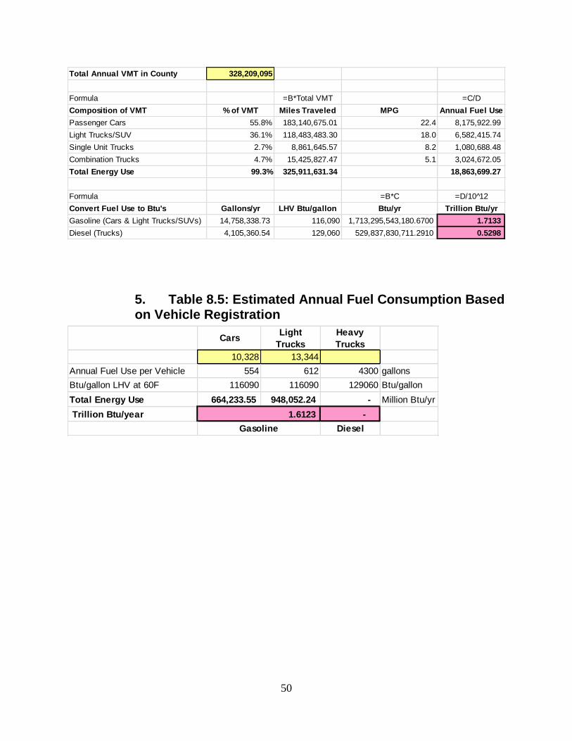
50
5. Table 8.5: Estimated Annual Fuel Consumption Based on Vehicle Registration
Total Annual VMT in County 328,209,095
Formula =B*Total VMT =C/D
Composition of VMT % of VMT Miles Traveled MPG Annual Fuel Use
Passenger Cars 55.8% 183,140,675.01 22.4 8,175,922.99
Light Trucks/SUV 36.1% 118,483,483.30 18.0 6,582,415.74
Single Unit Trucks 2.7% 8,861,645.57 8.2 1,080,688.48
Combination Trucks 4.7% 15,425,827.47 5.1 3,024,672.05
Total Energy Use 99.3% 325,911,631.34 18,863,699.27
Formula =B*C =D/10 1̂2
Convert Fuel Use to Btu's Gallons/yr LHV Btu/gallon Btu/yr Trillion Btu/yr
Gasoline (Cars & Light Trucks/SUVs) 14,758,338.73 116,090 1,713,295,543,180.6700 1.7133
Diesel (Trucks) 4,105,360.54 129,060 529,837,830,711.2910 0.5298
CarsLight
Trucks
Heavy
Trucks
10,328 13,344
Annual Fuel Use per Vehicle 554 612 4300 gallons
Btu/gallon LHV at 60F 116090 116090 129060 Btu/gallon
Total Energy Use 664,233.55 948,052.24 - Million Btu/yr
Trillion Btu/year 1.6123 -
DieselGasoline
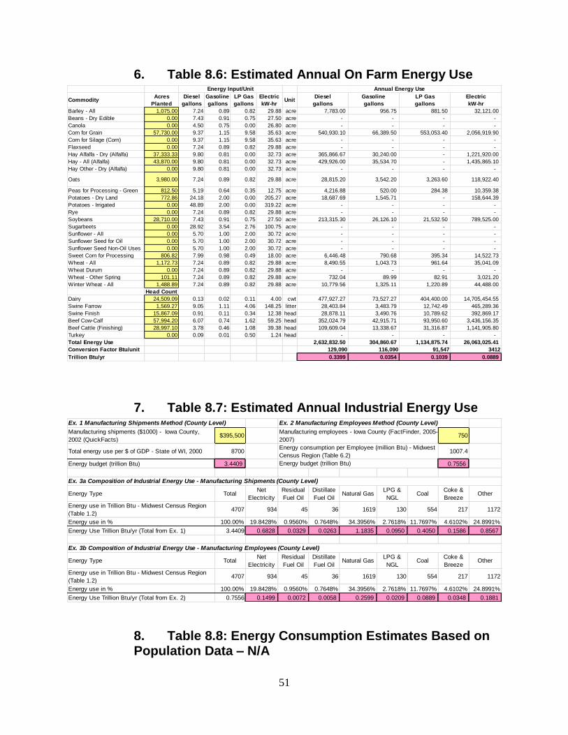
51
6. Table 8.6: Estimated Annual On Farm Energy Use
7. Table 8.7: Estimated Annual Industrial Energy Use
8. Table 8.8: Energy Consumption Estimates Based on Population Data – N/A
Barley - All 1,075.00 7.24 0.89 0.82 29.88 acre 7,783.00 956.75 881.50 32,121.00
Beans - Dry Edible 0.00 7.43 0.91 0.75 27.50 acre - - - -
Canola 0.00 4.50 0.75 0.00 26.80 acre - - - -
Corn for Grain 57,730.00 9.37 1.15 9.58 35.63 acre 540,930.10 66,389.50 553,053.40 2,056,919.90
Corn for Silage (Corn) 0.00 9.37 1.15 9.58 35.63 acre - - - -
Flaxseed 0.00 7.24 0.89 0.82 29.88 acre - - - -
Hay Alfalfa - Dry (Alfalfa) 37,333.33 9.80 0.81 0.00 32.73 acre 365,866.67 30,240.00 - 1,221,920.00
Hay - All (Alfalfa) 43,870.00 9.80 0.81 0.00 32.73 acre 429,926.00 35,534.70 - 1,435,865.10
Hay Other - Dry (Alfalfa) 0.00 9.80 0.81 0.00 32.73 acre - - - -
Oats 3,980.00 7.24 0.89 0.82 29.88 acre 28,815.20 3,542.20 3,263.60 118,922.40
Peas for Processing - Green 812.50 5.19 0.64 0.35 12.75 acre 4,216.88 520.00 284.38 10,359.38
Potatoes - Dry Land 772.86 24.18 2.00 0.00 205.27 acre 18,687.69 1,545.71 - 158,644.39
Potatoes - Irrigated 0.00 48.89 2.00 0.00 319.22 acre - - - -
Rye 0.00 7.24 0.89 0.82 29.88 acre - - - -
Soybeans 28,710.00 7.43 0.91 0.75 27.50 acre 213,315.30 26,126.10 21,532.50 789,525.00
Sugarbeets 0.00 28.92 3.54 2.76 100.75 acre - - - -
Sunflower - All 0.00 5.70 1.00 2.00 30.72 acre - - - -
Sunflower Seed for Oil 0.00 5.70 1.00 2.00 30.72 acre - - - -
Sunflower Seed Non-Oil Uses 0.00 5.70 1.00 2.00 30.72 acre - - - -
Sweet Corn for Processing 806.82 7.99 0.98 0.49 18.00 acre 6,446.48 790.68 395.34 14,522.73
Wheat - All 1,172.73 7.24 0.89 0.82 29.88 acre 8,490.55 1,043.73 961.64 35,041.09
Wheat Durum 0.00 7.24 0.89 0.82 29.88 acre - - - -
Wheat - Other Spring 101.11 7.24 0.89 0.82 29.88 acre 732.04 89.99 82.91 3,021.20
Winter Wheat - All 1,488.89 7.24 0.89 0.82 29.88 acre 10,779.56 1,325.11 1,220.89 44,488.00
Head Count
Dairy 24,509.09 0.13 0.02 0.11 4.00 cwt 477,927.27 73,527.27 404,400.00 14,705,454.55
Swine Farrow 1,569.27 9.05 1.11 4.06 148.25 litter 28,403.84 3,483.79 12,742.49 465,289.36
Swine Finish 15,867.09 0.91 0.11 0.34 12.38 head 28,878.11 3,490.76 10,789.62 392,869.17
Beef Cow-Calf 57,994.20 6.07 0.74 1.62 59.25 head 352,024.79 42,915.71 93,950.60 3,436,156.35
Beef Cattle (Finishing) 28,997.10 3.78 0.46 1.08 39.38 head 109,609.04 13,338.67 31,316.87 1,141,905.80
Turkey 0.00 0.09 0.01 0.50 1.24 head - - - -
Total Energy Use 2,632,832.50 304,860.67 1,134,875.74 26,063,025.41
Conversion Factor Btu/unit 129,090 116,090 91,547 3412
Trillion Btu/yr 0.3399 0.0354 0.1039 0.0889
LP Gas
gallons
Electric
kW-hr
Electric
kW-hrUnit
Diesel
gallons
Gasoline
gallonsCommodity
Annual Energy UseEnergy Input/Unit
Diesel
gallons
Acres
Planted
Gasoline
gallons
LP Gas
gallons
Manufacturing shipments ($1000) - Iowa County,
2002 (QuickFacts)$395,500 750
Total energy use per $ of GDP - State of WI, 2000 8700 1007.4
Energy budget (trillion Btu) 3.4409 0.7556
Energy Type TotalNet
Electricity
Residual
Fuel Oil
Distillate
Fuel OilNatural Gas
LPG &
NGLCoal
Coke &
BreezeOther
Energy use in Trillion Btu - Midwest Census Region
(Table 1.2)4707 934 45 36 1619 130 554 217 1172
Energy use in % 100.00% 19.8428% 0.9560% 0.7648% 34.3956% 2.7618% 11.7697% 4.6102% 24.8991%
Energy Use Trillion Btu/yr (Total from Ex. 1) 3.4409 0.6828 0.0329 0.0263 1.1835 0.0950 0.4050 0.1586 0.8567
Energy Type TotalNet
Electricity
Residual
Fuel Oil
Distillate
Fuel OilNatural Gas
LPG &
NGLCoal
Coke &
BreezeOther
Energy use in Trillion Btu - Midwest Census Region
(Table 1.2)4707 934 45 36 1619 130 554 217 1172
Energy use in % 100.00% 19.8428% 0.9560% 0.7648% 34.3956% 2.7618% 11.7697% 4.6102% 24.8991%
Energy Use Trillion Btu/yr (Total from Ex. 2) 0.7556 0.1499 0.0072 0.0058 0.2599 0.0209 0.0889 0.0348 0.1881
Energy budget (trillion Btu)
Ex. 3b Composition of Industrial Energy Use - Manufacturing Employees (County Level)
Ex. 1 Manufacturing Shipments Method (County Level)
Ex. 3a Composition of Industrial Energy Use - Manufacturing Shipments (County Level)
Ex. 2 Manufacturing Employees Method (County Level)
Manufacturing employees - Iowa County (FactFinder, 2005-
2007)
Energy consumption per Employee (million Btu) - Midwest
Census Region (Table 6.2)
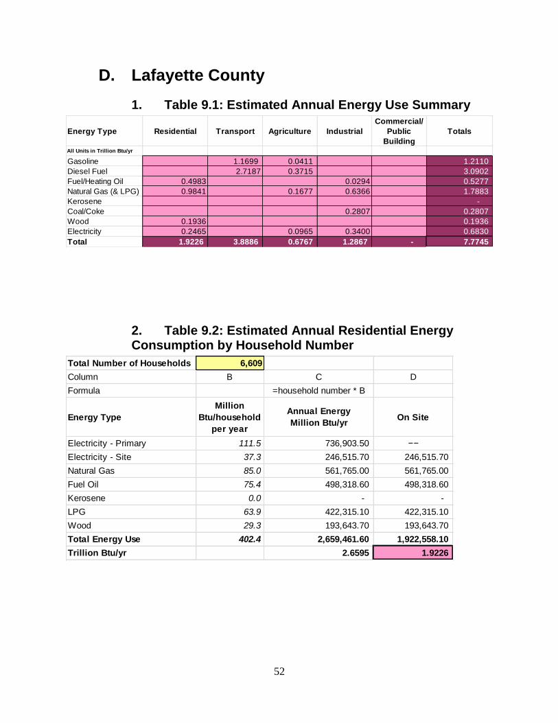
52
D. Lafayette County
1. Table 9.1: Estimated Annual Energy Use Summary
2. Table 9.2: Estimated Annual Residential Energy Consumption by Household Number
Energy Type Residential Transport Agriculture Industrial
Commercial/
Public
Building
Totals
All Units in Trillion Btu/yr
Gasoline 1.1699 0.0411 1.2110
Diesel Fuel 2.7187 0.3715 3.0902
Fuel/Heating Oil 0.4983 0.0294 0.5277
Natural Gas (& LPG) 0.9841 0.1677 0.6366 1.7883
Kerosene -
Coal/Coke 0.2807 0.2807
Wood 0.1936 0.1936
Electricity 0.2465 0.0965 0.3400 0.6830
Total 1.9226 3.8886 0.6767 1.2867 - 7.7745
Total Number of Households 6,609
Column B C D
Formula =household number * B
Energy Type
Million
Btu/household
per year
Annual Energy
Million Btu/yrOn Site
Electricity - Primary 111.5 736,903.50 −−
Electricity - Site 37.3 246,515.70 246,515.70
Natural Gas 85.0 561,765.00 561,765.00
Fuel Oil 75.4 498,318.60 498,318.60
Kerosene 0.0 - -
LPG 63.9 422,315.10 422,315.10
Wood 29.3 193,643.70 193,643.70
Total Energy Use 402.4 2,659,461.60 1,922,558.10
Trillion Btu/yr 2.6595 1.9226
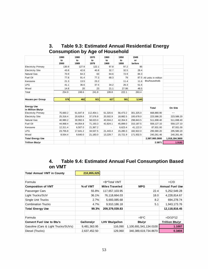
53
3. Table 9.3: Estimated Annual Residential Energy Consumption by Age of Household
4. Table 9.4: Estimated Annual Fuel Consumption Based on VMT
1990
to
2000
1980
to
1989
1970
to
1979
1960
to
1969
1950
to
1959
1949
or
before
Electricity Primary 130.9 127.9 122.1 97.8 97.2 85
Electricity Site 43.8 42.8 40.8 32.7 32.5 28.4
Natural Gas 70.9 64.3 63 64.6 72.9 84.3
Fuel Oil 77.8 91.4 77.3 68.3 79 87.5
Kerosene 21.3 13.5 23.2 11.4 11.6
LPG 41.1 36.6 37.5 34.2 26.3 51.6
Wood 14.8 20 23 21.1 27.06 48.5
Total 254.9 248.6 241.8 199.8 222.1 263.4
Houses per Group 578 482 921 627 581 3,545
Energy Use
in Million Btu/yrTotal On Site
Electricity Primary 75,660.2 61,647.8 112,454.1 61,320.6 56,473.2 301,325.0 668,880.90 −−
Electricity Site 25,316.4 20,629.6 37,576.8 20,502.9 18,882.5 100,678.0 223,586.20 223,586.20
Natural Gas 40,980.2 30,992.6 58,023.0 40,504.2 42,354.9 298,843.5 511,698.40 511,698.40
Fuel Oil 44,968.4 44,054.8 71,193.3 42,824.1 45,899.0 310,187.5 559,127.10 559,127.10
Kerosene 12,311.4 6,507.0 21,367.2 - 6,623.4 41,122.0 87,931.00 87,931.00
LPG 23,755.8 17,641.2 34,537.5 21,443.4 15,280.3 182,922.0 295,580.20 295,580.20
Wood 8,554.4 9,640.0 21,183.0 13,229.7 15,721.9 171,932.5 240,261.46 240,261.46
Total Energy Use 2,587,065.2600 1,918,184.3600
Trillion Btu/yr 2.5871 1.9182
All units in million
Btu/household.
Total Annual VMT in County 210,855,025
Formula =B*Total VMT =C/D
Composition of VMT % of VMT Miles Traveled MPG Annual Fuel Use
Passenger Cars 55.8% 117,657,103.95 22.4 5,252,549.28
Light Trucks/SUV 36.1% 76,118,664.03 18.0 4,228,814.67
Single Unit Trucks 2.7% 5,693,085.68 8.2 694,278.74
Combination Trucks 4.7% 9,910,186.18 5.1 1,943,173.76
Total Energy Use 99.3% 209,379,039.83 12,118,816.45
Formula =B*C =D/10 1̂2
Convert Fuel Use to Btu's Gallons/yr LHV Btu/gallon Btu/yr Trillion Btu/yr
Gasoline (Cars & Light Trucks/SUVs) 9,481,363.95 116,090 1,100,691,541,134.0100 1.1007
Diesel (Trucks) 2,637,452.50 129,060 340,389,619,734.8670 0.3404

54
Barley - All 0.00 7.24 0.89 0.82 29.88 acre - - - -
Beans - Dry Edible 0.00 7.43 0.91 0.75 27.50 acre - - - -
Canola 0.00 4.50 0.75 0.00 26.80 acre - - - -
Corn for Grain 127,200.00 9.37 1.15 9.58 35.63 acre 1,191,864.00 146,280.00 1,218,576.00 4,532,136.00
Corn for Silage (Corn) 0.00 9.37 1.15 9.58 35.63 acre - - - -
Flaxseed 0.00 7.24 0.89 0.82 29.88 acre - - - -
Hay Alfalfa - Dry (Alfalfa) 0.00 9.80 0.81 0.00 32.73 acre - - - -
Hay - All (Alfalfa) 43,785.00 9.80 0.81 0.00 32.73 acre 429,093.00 35,465.85 - 1,433,083.05
Hay Other - Dry (Alfalfa) 0.00 9.80 0.81 0.00 32.73 acre - - - -
Oats 4,013.00 7.24 0.89 0.82 29.88 acre 29,054.12 3,571.57 3,290.66 119,908.44
Peas for Processing - Green 0.00 5.19 0.64 0.35 12.75 acre - - - -
Potatoes - Dry Land 0.00 24.18 2.00 0.00 205.27 acre - - - -
Potatoes - Irrigated 0.00 48.89 2.00 0.00 319.22 acre - - - -
Rye 0.00 7.24 0.89 0.82 29.88 acre - - - -
Soybeans 49,467.00 7.43 0.91 0.75 27.50 acre 367,539.81 45,014.97 37,100.25 1,360,342.50
Sugarbeets 0.00 28.92 3.54 2.76 100.75 acre - - - -
Sunflower - All 0.00 5.70 1.00 2.00 30.72 acre - - - -
Sunflower Seed for Oil 0.00 5.70 1.00 2.00 30.72 acre - - - -
Sunflower Seed Non-Oil Uses 0.00 5.70 1.00 2.00 30.72 acre - - - -
Sweet Corn for Processing 0.00 7.99 0.98 0.49 18.00 acre - - - -
Wheat - All 0.00 7.24 0.89 0.82 29.88 acre - - - -
Wheat Durum 0.00 7.24 0.89 0.82 29.88 acre - - - -
Wheat - Other Spring 0.00 7.24 0.89 0.82 29.88 acre - - - -
Winter Wheat - All 1,775.00 7.24 0.89 0.82 29.88 acre 12,851.00 1,579.75 1,455.50 53,037.00
Head Count
Dairy 30,100.00 0.13 0.02 0.11 4.00 cwt 586,950.00 90,300.00 496,650.00 18,060,000.00
Swine Farrow 9.05 1.11 4.06 148.25 litter - - - -
Swine Finish 0.91 0.11 0.34 12.38 head - - - -
Beef Cow-Calf 6.07 0.74 1.62 59.25 head - - - -
Beef Cattle (Finishing) 68,838.00 3.78 0.46 1.08 39.38 head 260,207.64 31,665.48 74,345.04 2,710,840.44
Turkey 0.09 0.01 0.50 1.24 head - - - -
Total Energy Use 2,877,559.57 353,877.62 1,831,417.45 28,269,347.43
Conversion Factor Btu/unit 129,090 116,090 91,547 3412
Trillion Btu/yr 0.3715 0.0411 0.1677 0.0965
LP Gas
gallons
Electric
kW-hr
Electric
kW-hrUnit
Diesel
gallons
Gasoline
gallonsCommodity
Annual Energy UseEnergy Input/Unit
Diesel
gallons
Acres
Planted
Gasoline
gallons
LP Gas
gallons
5. Table 9.5: Estimated Annual Fuel Consumption Based on Vehicle Registration
6. Table 9.6: Estimated Annual On Farm Energy Use
CarsLight
Trucks
Heavy
Trucks
7,102 10,038 4,899
Annual Fuel Use per Vehicle 554 612 4300 gallons
Btu/gallon LHV at 60F 116090 116090 129060 Btu/gallon
Total Energy Use 456,757.03 713,170.59 2,718,739.24 Million Btu/yr
Trillion Btu/year 1.1699 2.7187
DieselGasoline

55
7. Table 9.7: Estimated Annual Industrial Energy Use
8. Table 9.8: Energy Consumption Estimates Based on Population Data
E. Richland County
1. Table 10.1: Estimated Annual Energy Use Summary
Manufacturing shipments ($1000) - Lafayette County,
2007 (QuickFacts)209,683
1635
Total energy use per $ of GDP - State of WI, 2010 316.6 1007.4
Energy budget (trillion Btu) 0.0664 1.6471
Energy Type TotalNet
Electricity
Residual
Fuel Oil
Distillate
Fuel Oil
Natural
Gas
LPG &
NGLCoal
Coke &
BreezeOther
Energy use in Trillion Btu - Midwest Census Region
(Table 1.2)4707 934 45 36 1619 130 554 217 1172
Energy use in % 100.00% 19.8428% 0.9560% 0.7648% 34.3956% 2.7618% 11.7697% 4.6102% 24.8991%
Energy Use Trillion Btu/yr (Total from Ex. 1) 0.0664 0.0132 0.0006 0.0005 0.0228 0.0018 0.0078 0.0031 0.0165
Energy Type TotalNet
Electricity
Residual
Fuel Oil
Distillate
Fuel Oil
Natural
Gas
LPG &
NGLCoal
Coke &
BreezeOther
Energy use in Trillion Btu - Midwest Census Region
(Table 1.2)4707 934 45 36 1619 130 554 217 1172
Energy use in % 100.00% 19.8428% 0.9560% 0.7648% 34.3956% 2.7618% 11.7697% 4.6102% 24.8991%
Energy Use Trillion Btu/yr (Total from Ex. 2) 1.6471 0.3268 0.0157 0.0126 0.5665 0.0455 0.1939 0.0759 0.4101
Energy budget (trillion Btu)
Ex. 3b Composition of Industrial Energy Use - Manufacturing Employees (County Level)
Ex. 1 Manufacturing Shipments Method (County Level)
Ex. 3a Composition of Industrial Energy Use - Manufacturing Shipments (County Level)
Ex. 2 Manufacturing Employees Method (County Level)
Manufacturing employees - Lafayette County
(FactFinder, 2005-2007)
Energy consumption per Employee (million Btu) -
Midwest Census Region (Table 6.2)
Population % of WI WI 426.4000 355.4000 459.3000 402.6000 1643.7000
Lafayette 16815 0.2944% Residential Commercial Industrial Transportation Total
0.0000% Lafayette 1.2553 1.0463 1.3521 1.1852 4.8389
WI 5,711,767 100.0000% Lafayette 1.2553 1.0463 1.3521 1.1852 4.8389
WI 353.5 Million Btu/Capita
WI 499 391.4 470.8 319.9
Million Btu Trillion Btu Coal Natural Gas Petroleum Electricity Total
Lafayette 5944103 5.9441 Lafayette 1.4690 1.1523 1.3860 0.9418 4.9490
Total Energy Per Capita Consumption
Population Makeup Energy Consumption by Sector (Trillion Btu)
Energy Consumption by Source (Trillion Btu)
Energy Type Residential Transport Agriculture Industrial
Commercial
/
Public
Building
Totals
All Units in Trillion Btu/yr
Gasoline 0.0003 0.0190 0.0193
Diesel Fuel 0.0001 0.1721 0.1722
Fuel/Heating Oil 0.0001 0.1146 0.1147
Natural Gas (& LPG) 0.0001 0.0699 2.4742 0.0851 2.6293
Kerosene -
Coal/Coke 1.0907 1.0907
Wood 0.0000 0.0000
Electricity 0.0001 0.0493 1.3213 0.0860 1.4567
Total 0.0003 0.0004 0.3103 5.0008 0.1711 5.4829
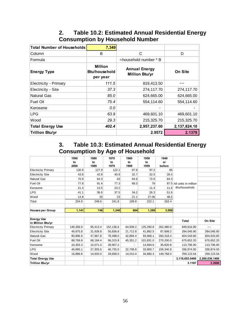
56
2. Table 10.2: Estimated Annual Residential Energy Consumption by Household Number
3. Table 10.3: Estimated Annual Residential Energy Consumption by Age of Household
Total Number of Households 7,349
Column B C D
Formula =household number * B
Energy Type
Million
Btu/household
per year
Annual Energy
Million Btu/yrOn Site
Electricity - Primary 111.5 819,413.50 −−
Electricity - Site 37.3 274,117.70 274,117.70
Natural Gas 85.0 624,665.00 624,665.00
Fuel Oil 75.4 554,114.60 554,114.60
Kerosene 0.0 - -
LPG 63.9 469,601.10 469,601.10
Wood 29.3 215,325.70 215,325.70
Total Energy Use 402.4 2,957,237.60 2,137,824.10
Trillion Btu/yr 2.9572 2.1378
1990
to
2000
1980
to
1989
1970
to
1979
1960
to
1969
1950
to
1959
1949
or
before
Electricity Primary 130.9 127.9 122.1 97.8 97.2 85
Electricity Site 43.8 42.8 40.8 32.7 32.5 28.4
Natural Gas 70.9 64.3 63 64.6 72.9 84.3
Fuel Oil 77.8 91.4 77.3 68.3 79 87.5
Kerosene 21.3 13.5 23.2 11.4 11.6
LPG 41.1 36.6 37.5 34.2 26.3 51.6
Wood 14.8 20 23 21.1 27.06 48.5
Total 254.9 248.6 241.8 199.8 222.1 263.4
Houses per Group 1,141 746 1,246 664 1,289 3,088
Energy Use
in Million Btu/yrTotal On Site
Electricity Primary 149,356.9 95,413.4 152,136.6 64,939.2 125,290.8 262,480.0 849,616.90 −−
Electricity Site 49,975.8 31,928.8 50,836.8 21,712.8 41,892.5 87,699.2 284,045.90 284,045.90
Natural Gas 80,896.9 47,967.8 78,498.0 42,894.4 93,968.1 260,318.4 604,543.60 604,543.60
Fuel Oil 88,769.8 68,184.4 96,315.8 45,351.2 101,831.0 270,200.0 670,652.20 670,652.20
Kerosene 24,303.3 10,071.0 28,907.2 - 14,694.6 35,820.8 113,796.90 113,796.90
LPG 46,895.1 27,303.6 46,725.0 22,708.8 33,900.7 159,340.8 336,874.00 336,874.00
Wood 16,886.8 14,920.0 28,658.0 14,010.4 34,880.3 149,768.0 259,123.54 259,123.54
Total Energy Use 3,118,653.0400 2,269,036.1400
Trillion Btu/yr 3.1187 2.2690
All units in million
Btu/household.
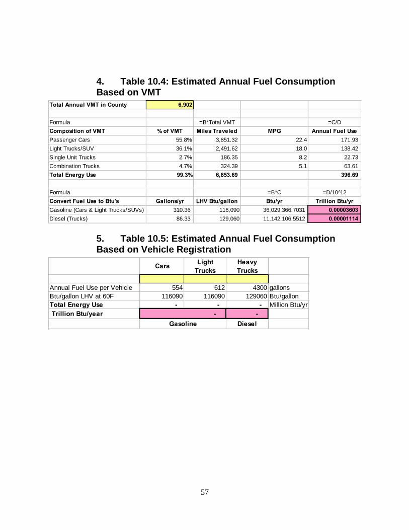
57
4. Table 10.4: Estimated Annual Fuel Consumption Based on VMT
5. Table 10.5: Estimated Annual Fuel Consumption Based on Vehicle Registration
Total Annual VMT in County 6,902
Formula =B*Total VMT =C/D
Composition of VMT % of VMT Miles Traveled MPG Annual Fuel Use
Passenger Cars 55.8% 3,851.32 22.4 171.93
Light Trucks/SUV 36.1% 2,491.62 18.0 138.42
Single Unit Trucks 2.7% 186.35 8.2 22.73
Combination Trucks 4.7% 324.39 5.1 63.61
Total Energy Use 99.3% 6,853.69 396.69
Formula =B*C =D/10 1̂2
Convert Fuel Use to Btu's Gallons/yr LHV Btu/gallon Btu/yr Trillion Btu/yr
Gasoline (Cars & Light Trucks/SUVs) 310.36 116,090 36,029,366.7031 0.00003603
Diesel (Trucks) 86.33 129,060 11,142,106.5512 0.00001114
CarsLight
Trucks
Heavy
Trucks
Annual Fuel Use per Vehicle 554 612 4300 gallons
Btu/gallon LHV at 60F 116090 116090 129060 Btu/gallon
Total Energy Use - - - Million Btu/yr
Trillion Btu/year - -
DieselGasoline

58
6. Table 10.6: Estimated Annual On Farm Energy Use
7. Table 10.7: Estimated Annual Industrial Energy Use
Barley - All 7.24 0.89 0.82 29.88 acre - - - -
Beans - Dry Edible 7.43 0.91 0.75 27.50 acre - - - -
Canola 4.50 0.75 0.00 26.80 acre - - - -
Corn for Grain 45,000.00 9.37 1.15 9.58 35.63 acre 421,650.00 51,750.00 431,100.00 1,603,350.00
Corn for Silage (Corn) 9.37 1.15 9.58 35.63 acre - - - -
Flaxseed 7.24 0.89 0.82 29.88 acre - - - -
Hay Alfalfa - Dry (Alfalfa) 22,600.00 9.80 0.81 0.00 32.73 acre 221,480.00 18,306.00 - 739,698.00
Hay - All (Alfalfa) 9.80 0.81 0.00 32.73 acre - - - -
Hay Other - Dry (Alfalfa) 9.80 0.81 0.00 32.73 acre - - - -
Oats 2,600.00 7.24 0.89 0.82 29.88 acre 18,824.00 2,314.00 2,132.00 77,688.00
Peas for Processing - Green 5.19 0.64 0.35 12.75 acre - - - -
Potatoes - Dry Land 24.18 2.00 0.00 205.27 acre - - - -
Potatoes - Irrigated 48.89 2.00 0.00 319.22 acre - - - -
Rye 7.24 0.89 0.82 29.88 acre - - - -
Soybeans 11,800.00 7.43 0.91 0.75 27.50 acre 87,674.00 10,738.00 8,850.00 324,500.00
Sugarbeets 28.92 3.54 2.76 100.75 acre - - - -
Sunflower - All 5.70 1.00 2.00 30.72 acre - - - -
Sunflower Seed for Oil 5.70 1.00 2.00 30.72 acre - - - -
Sunflower Seed Non-Oil Uses 5.70 1.00 2.00 30.72 acre - - - -
Sweet Corn for Processing 7.99 0.98 0.49 18.00 acre - - - -
Wheat - All 7.24 0.89 0.82 29.88 acre - - - -
Wheat Durum 7.24 0.89 0.82 29.88 acre - - - -
Wheat - Other Spring 7.24 0.89 0.82 29.88 acre - - - -
Winter Wheat - All 1,300.00 7.24 0.89 0.82 29.88 acre 9,412.00 1,157.00 1,066.00 38,844.00
Head Count
Dairy 14,800.00 0.13 0.02 0.11 4.00 cwt 288,600.00 44,400.00 244,200.00 8,880,000.00
Swine Farrow 9.05 1.11 4.06 148.25 litter - - - -
Swine Finish 0.91 0.11 0.34 12.38 head - - - -
Beef Cow-Calf 47,000.00 6.07 0.74 1.62 59.25 head 285,290.00 34,780.00 76,140.00 2,784,750.00
Beef Cattle (Finishing) 3.78 0.46 1.08 39.38 head - - - -
Turkey 0.09 0.01 0.50 1.24 head - - - -
Total Energy Use 1,332,930.00 163,445.00 763,488.00 14,448,830.00
Conversion Factor Btu/unit 129,090 116,090 91,547 3412
Trillion Btu/yr 0.1721 0.0190 0.0699 0.0493
Energy Input/Unit Annual Energy Use
CommodityAcres
Planted
Diesel
gallons
Gasolin
e
LP Gas
gallons
Electric
kW-hrUnit
Diesel
gallons
Gasoline
gallons
LP Gas
gallons
Electric
kW-hr
Manufacturing shipments ($1000) - Becker County,
2002 (QuickFacts)$613,108 1315
Total energy use per $ of GDP - State of MN, 2000 8700 1007.4
Energy budget (trillion Btu) 5.3340 1.3247
Energy Type TotalNet
Electricity
Residual
Fuel Oil
Distillate
Fuel Oil
Natural
Gas
LPG &
NGLCoal
Coke &
BreezeOther
Energy use in Trillion Btu - Midwest Census Region
(Table 1.2)4707 934 45 36 1619 130 554 217 1172
Energy use in % 100.00% 19.8428% 0.9560% 0.7648% 34.3956% 2.7618% 11.7697% 4.6102% 24.8991%
Energy Use Trillion Btu/yr (Total from Ex. 1) 5.3340 1.0584 0.0510 0.0408 1.8347 0.1473 0.6278 0.2459 1.3281
Energy Type TotalNet
Electricity
Residual
Fuel Oil
Distillate
Fuel Oil
Natural
Gas
LPG &
NGLCoal
Coke &
BreezeOther
Energy use in Trillion Btu - Midwest Census Region
(Table 1.2)4707 934 45 36 1619 130 554 217 1172
Energy use in % 100.00% 19.8428% 0.9560% 0.7648% 34.3956% 2.7618% 11.7697% 4.6102% 24.8991%
Energy Use Trillion Btu/yr (Total from Ex. 2) 1.3247 0.2629 0.0127 0.0101 0.4556 0.0366 0.1559 0.0611 0.3298
Ex. 1 Manufacturing Shipments Method (County Level) Ex. 2 Manufacturing Employees Method (County Level)
Manufacturing employees - Becker County (FactFinder,
2005-2007)
Energy consumption per Employee (million Btu) -
Midwest Census Region (Table 6.2)
Energy budget (trillion Btu)
Ex. 3a Composition of Industrial Energy Use - Manufacturing Shipments (County Level)
Ex. 3b Composition of Industrial Energy Use - Manufacturing Employees (County Level)

59
8. Table 10.8: Energy Consumption Estimates Based on Population Data
Population % of MN WI 427.6610 351.9980 577.3140 443.1000 1800.0730
Richland County 18021 0.3169% Residential Commercial Industrial Transportation Total
0.0000% Richland 1.3552 1.1154 1.8294 1.4041 5.7041
0.0000% 0.0000 0.0000 0.0000 0.0000 0.0000
0.0000% 0.0000 0.0000 0.0000 0.0000 0.0000
Four Counties 18021 0.3169% 0.0000 0.0000 0.0000 0.0000 0.0000
WI 5,686,986 100.0000% Four Counties 1.3552 1.1154 1.8294 1.4041 5.7041
WI 353.5 Million Btu/Capita
WI 25.517 372.916 104.5
Million Btu Trillion Btu Coal Natural Gas Petroleum Electricity Total
Richland 5694636 5.6946 Richland 0.0809 1.1817 0.3311 0.0000 1.5937
0 0.0000 0.0000 0.0000 0.0000 0.0000 0.0000
0 0.0000 0.0000 0.0000 0.0000 0.0000 0.0000
0 0.0000 0.0000 0.0000 0.0000 0.0000 0.0000
Four Counties 5694636 5.6946 Four Counties 0.0809 1.1817 0.3311 0.0000 1.5937
Energy Consumption by Source (Trillion Btu)
Total Energy Per Capita Consumption
Population Makeup Energy Consumption by Sector (Trillion Btu)


