Page 1
REPORTS OF THE TIBOR T. POLGAR
FELLOWSHIP PROGRAM, 2016
Sarah H. Fernald, David J. Yozzo
and Helena Andreyko
Editors
A Joint Program of
The Hudson River Foundation
and The New York State
Department of Environmental Conservation
January 2019
Page 3
iii
ABSTRACT
Seven studies completed within the Hudson River Estuary under the auspices of the
Tibor T. Polgar Fellowship Program during 2016 have been included in the current volume.
Major objectives of these studies included: (1) distinguishing sources of fecal bacteria in six
Hudson River tributaries through DNA profiles, (2) using the Regional Ocean Modeling
System (ROMS) to predict potential phytoplankton blooms in the Hudson River Estuary, (3)
gathering baseline information about submersed aquatic vegetation communities in New
York’s Great Swamp, (4) investigating the linkage between sediment metal, metal
accumulation, and induction of metallothionein, comparing grass shrimp from pristine and
contaminated sites, (5) examining the role of aryl hydrocarbon receptor 2 (AHR2) in TCDD
toxicity associated with cardiac pathologies in tomcod, (6) determining the impact of perched
culverts on upstream migration of American eel, and (7) examining the correlation between
land use and microplastic content in four Hudson River tributaries.
Page 5
v
TABLE OF CONTENTS
Abstract ............................................................................................................... iii
Preface ................................................................................................................. vii
Fellowship Reports
Utilizing DNA Sequencing and Land Use Data for an Improved Understanding
of Fecal Contamination in Hudson River Tributaries
Elizabeth P. Farrell and Gregory D. O’Mullan .................................................... I-1
Modeling Potential Phytoplankton Blooms in the Hudson River Estuary:
Challenges and Solutions
Samuel A. Nadell and Robert W. Howarth.......................................................... II-1
Submersed Aquatic Vegetation in a Hudson River Watershed: The Great Swamp
of New York
Chris Cotroneo and John Waldman ..................................................................... III-1
Induction of Metallothionein in Grass Shrimp (Palaemonetes pugio) Exposed to
Naturally Occurring Metals
Abhishek Naik and William G. Wallace .............................................................. IV-1
Quantifying the Effects of TCDD Exposure on Early Life-Stage Cardiac Gene
Expression of Atlantic Tomcod by RT-PCR
Kristy A. Vitale and Isaac Wirgin........................................................................ V-1
Perched Culverts’ Effects on Downstream Eel Habitat in Hudson River Streams
Marissa J. Porter, Zofia Gagnon, Robert Schmidt, and Christopher Bowser ...... VI-1
Effects of Tributaries in the Transport of Microplastics in the Hudson Valley
Watershed
Ian Krout, Zofia Gagnon, David Conover, and Christopher Bowser .................. VII-1
Page 7
vii
PREFACE
The Hudson River estuary stretches from its tidal limit at the Federal Dam at Troy,
New York, to its merger with the New York Bight, south of New York City. Within that
reach, the estuary displays a broad transition from tidal freshwater to marine conditions that
are reflected in its physical composition and the biota its supports. As such, it presents a
major opportunity and challenge to researchers to describe the makeup and workings of a
complex and dynamic ecosystem. The Tibor T. Polgar Fellowship Program provides funds
for students to study selected aspects of the physical, chemical, biological, and public policy
realms of the estuary.
The Polgar Fellowship Program was established in 1985 in memory of Dr. Tibor T.
Polgar, former Chairman of the Hudson River Foundation Science Panel. The 2016 program
was jointly conducted by the Hudson River Foundation for Science and Environmental
Research and the New York State Department of Environmental Conservation and
underwritten by the Hudson River Foundation. The fellowship program provides stipends
and research funds for research projects within the Hudson drainage basin and is open to
graduate and undergraduate students.
Page 8
viii
Prior to 1988, Polgar studies were conducted only within the four sites that comprise
the Hudson River National Estuarine Research Reserve, a part of the National Estuarine
Research Reserve System. The four Hudson River sites, Piermont Marsh, Iona Island, Tivoli
Bays, and Stockport Flats exceed 4,000 acres and include a wide variety of habitats spaced
over 100 miles of the Hudson estuary. Since 1988, the Polgar Program has supported
research carried out at any location within the Hudson estuary.
The work reported in this volume represents seven research projects conducted by
Polgar Fellows during 2016. These studies meet the goals of the Tibor T. Polgar Fellowship
Program to generate new information on the nature of the Hudson estuary and to train
students in estuarine science.
Sarah H. Fernald
New York State Department of Environmental Conservation
Hudson River National Estuarine Research Reserve
David J. Yozzo
Glenford Environmental Science
Helena Andreyko
Hudson River Foundation for Science and Environmental Research
Page 9
I-1
UTILIZING DNA SEQUENCING AND LAND USE DATA FOR AN IMPROVED
UNDERSTANDING OF FECAL CONTAMINATION IN HUDSON RIVER
TRIBUTARIES
A Final Report of the Tibor T. Polgar Fellowship Program
Elizabeth P. Farrell
Polgar Fellow
School for Earth and Environmental Sciences
CUNY Queens College
Flushing, NY 11367
Project Advisor:
Dr. Gregory D. O’Mullan
School for Earth and Environmental Sciences
CUNY Queens College
Flushing, NY 11367
Farrell, E. P. and G. D. O’Mullan. 2019. Utilizing DNA Sequencing and Land Use Data for an
Improved Understanding of Fecal Contamination in Hudson River Tributaries, Section I: 1-25 pp. In
S.H. Fernald, D.J. Yozzo, and H. Andreyko (eds.), Final Reports of the Tibor T. Polgar Fellowship
Program, 2016. Hudson River Foundation.
Page 10
I-2
ABSTRACT
Tributary mixing zones into the Hudson represent areas of both the highest
frequency and magnitude of fecal indicator bacteria (FIB) contamination. The frequency
and magnitude of contamination vary among tributaries and it is hypothesized that this
indicates differing fecal sources. While EPA approved cultivation-based methods for the
enumeration of FIB provide powerful tools for watershed monitoring, mitigation
decisions require additional information related to the source of fecal bacteria. Data from
cultivation based FIB and microbial community profiles based on high throughput DNA
sequencing were analyzed in combination with land use patterns to better understand the
sources of fecal contamination in six tributaries.
Land use patterns provided useful insights to begin understanding FIB patterns.
On a watershed scale, forested areas were negatively correlated with FIB contamination,
while developed areas had a positive correlation. The arrangement of site specific land
use, ordered upstream to downstream, was often observed to influence the extent of FIB
contamination. DNA sequencing data from a subset of sites was used to identify
potential sewage and fecal contributions using a broader microbial community
perspective for comparison to the patterns obtained from the commonly used, but
taxonomically restricted cultivation-based fecal indicator, enterococci. The ratio of
sewage to fecal microbial signatures varied among tributaries, possibly non-uniform
sources, including fluctuating spatial contributions of human and animal sources. A
diverse combination of monitoring tools should be developed and utilized, to provide
complementary information toward improved differentiation of contamination sources
and optimized mitigation actions for effective water quality management.
Page 11
I-3
TABLE OF CONTENTS
Abstract ................................................................................................................ I-2
Table of Contents ................................................................................................. I-3
Lists of Figures and Tables .................................................................................. I-4
Introduction .......................................................................................................... I-5
Methods................................................................................................................ I-9
Fecal Indicators and Microbial Community Data .................................... I-9
Land Cover Database and GIS Analysis of FIB Data.............................. I-10
Results and Discussion ........................................................................................ I-13
Conclusions .......................................................................................................... I-20
Acknowledgements .............................................................................................. I-21
References ............................................................................................................ I-22
Page 12
I-4
LIST OF FIGURES AND TABLES
Figure 1 – Sampling Sites Across Tributaries of the Hudson River .................... I-9
Table 1 – Simplification of Land Use Classifications ......................................... I-11
Figure 2 – GM ENT Levels by Tributary ............................................................ I-13
Figure 3 – Percent Land Use by Tributary ........................................................... I-13
Figure 4 – Percent Low to High Intensity Developed Land Use ......................... I-14
Figure 5 – Percent Forested Land Use ................................................................. I-14
Figure 6 – ENT, Land Use and DNA data in Sparkill: 3 Potential Zones
of Impact ............................................................................................ I-15
Figure 7 – ENT, Land Use and DNA data in Pocantico ...................................... I-16
Figure 8 – ENT, Land Use and DNA data in Wallkill ........................................ I-16
Figure 9 – ENT response to land use in Rondout (River Mile 0-28) ................... I-17
Figure 10 – ENT response to land use in Rondout (River Mile 28-42) ............... I-18
Figure 11 – ENT response to land use in Catskill ............................................... I-18
Page 13
I-5
INTRODUCTION
Studying fecal contamination in the Hudson River tributaries is important for
addressing potential public health risks, water resource management and habitat
preservation. The Hudson’s tributaries deliver water, nutrients, and sediment to the
estuary while providing habitats for wildlife and for resident and migratory fish (NYS
DEC 2015). Relatively little information is available regarding how land use in the
watershed impacts the integrity and resiliency of the estuary. As the Hudson River
Estuary Program action agenda endeavors to improve water quality by reducing
pathogens (NYS DEC 2015), that connection between land use and the overall health of
the estuary should be explored. Research that increases the understanding of important
connections among land, tributaries, and the estuary can provide knowledge to better
inform management actions that provide the greatest benefit to the health and resiliency
of the estuary (NYS DEC 2015). Many Hudson tributaries contain very high levels of the
Fecal Indicator Bacteria (FIB) enterococci (ENT) (Young et al. 2013; Suter et al. 2011),
with 72% of citizen science samples (Riverkeeper 2015) exceeding the EPA’s
recommended Beach Action Value (BAV) of 60 ENT cells/100ml (USEPA 2012).
Tributary mixing zones into the Hudson represent both the highest frequency (frequency
of exceeding BAV) and magnitude (geometric mean by site) of FIB contamination, as
compared to mid-channel, nearshore, and even wastewater treatment plant outfalls (Suter
et al. 2011; Riverkeeper 2014). Understanding the sources of contamination in the
tributaries is critical to deciphering patterns of fecal bacterial contamination of the
Hudson River Estuary as a whole.
Page 14
I-6
Fecal indicator bacteria (FIB), including ENT, are used to assess the combined
extent of fecal contamination which can originate from numerous pollution sources,
including human sewage, manure from livestock operations, wildlife, and urban runoff
(Boehm et al. 2013). Ecosystems in developed areas possess a multitude of delivery
mechanisms which often contain multiple fecal sources, making it extremely difficult to
mitigate the pollution (Newton et al. 2013; O’Mullan et al. 2017). ENT measurements
are not as useful when there is evidence of chronic contamination and sources need to be
identified to address the problem (McLellan and Eren 2014). Human specific fecal
pollution can originate from a variety of sources such as leaky or damaged sanitary sewer
lines, faulty septic systems, illicit waste disposal, and sanitary/combined sewer overflows
(Eaton et al. 2013). As a result, the characterization and management of human fecal
pollution is closely linked with local waste management practices, adjacent land use,
precipitation, and wet weather hydrology (Peed et al. 2011). Traditional culture-based
methods, while commonly used to characterize fecal pollution, do not discern between
human and other animal sources of fecal pollution. While FIB concentrations are
essential tools for contamination assessment and the application of water quality
regulations, management and mitigation efforts would benefit from the use of additional
water quality research options.
Microorganisms that thrive within sewer systems may serve as useful adjuncts to
fecal indicators for tracking sewage contamination because they could provide a
signature of sewage pollution in surface waters (VandeWalle et al. 2012). These
microbial sewage communities consist of a combination of human fecal microorganisms
and non-fecal microorganisms which reside in the sewer infrastructure (Shanks et al.
Page 15
I-7
2013). The advent of molecular methods allows for non-cultured organisms to be used as
alternative fecal indicators (McLellan and Eren 2014), and these approaches have become
popular and efficient methods for characterizing and tracking changes in the community
structures of microbial populations (Bernhard and Field 2000). High throughput
metagenomic DNA sequencing approaches can be used to evaluate the community
signature from broader groups of fecal associated microbes. These broader groups of
fecal associated microbes are what the traditional cultivation based FIB aim to indicate.
There are several factors that differ between the Hudson and its tributaries. One
obvious dissimilarity is the scale of the bodies of water: in tributaries, a smaller volume
of fecal or sewage input can have a larger spatial impact than in larger systems such as
the Hudson, due to a reduction in the dilution of contaminants. Above the head of tide,
the tributaries also have highly variable discharge rates and unidirectional flow, unlike
the tributary mouths and main-stem Hudson, which are tidally influenced. These factors
may lead to contamination remaining more localized in the Hudson, whereas in the
tributaries the concentration of contaminants may be higher and contaminants may be
transported larger distances downstream. In addition, sprawling development patterns
can have negative consequences, including, but not limited to, the contribution of excess
pollutants, nutrients and sediment to tributaries and the estuary (NYS DEC 2015).
Development can increase the amount of impervious surfaces and result in increases in
stormwater flows (NYS DEC 2015). Impervious surface coverage has been positively
correlated with fecal bacterial contamination in freshwater urban streams (Young and
Thackson 1999) and tidal creek ecosystems (Mallin et al. 2000; Holland et al. 2004). A
1999 study showed that the concentration of certain pathogens, including ENT, were
Page 16
I-8
directly related to the housing density, population, development, imperviousness, and
apparent animal density (Selvakumar and Borst 2006). Surface runoff samples from
more densely populated, sewered areas regularly reflected higher bacterial counts when
compared to runoff from less developed areas with septic tanks, which suggests that a
relationship may exist between land use and potential bacterial loading (Young and
Thackson 1999). The majority of larger rivers are influenced by hundreds of small
streams draining from multiple watersheds which can make it particularly difficult to
associate a specific land use scenario with poor water quality (Peed et al. 2011).
Prior monitoring activities have identified tributaries to be both hot spots of fecal
contamination and an important determinant of water quality in the Hudson River itself.
Ultimately, source identification and remediation of contamination rather than merely
detection will protect public health and improve recreational opportunities afforded by
our natural resources. In order to better understand the patterns and causes of tributary
fecal contamination, the objectives of this study were to: 1) analyze existing culture based
FIB data to identify spatial patterns in contamination; 2) analyze available DNA
sequences from tributaries to investigate the spatial changes in the potential influence of
“fecal” and “sewage infrastructure” microorganisms on tributary water quality; 3) assess
land use patterns to determine if they can provide insight into patterns of FIB; and 4)
examine the effectiveness of a combination of monitoring tools for improved information
to differentiate between sources of contamination. As the frequency and magnitude of
contamination was known to vary among tributaries, it was hypothesized that the sources
of fecal contamination were also likely to differ among tributaries.
Page 17
I-9
METHODS
Fecal Indicators and Microbial Community Data
Citizen science FIB data, collected following EPA approved methods (USEPA
2012) from 110 sites along the Catskill, Esopus,
Rondout, Wallkill, Sparkill and Pocantico tributaries
(Figure 1), were obtained from Riverkeeper
(www.riverkeeper.org; Riverkeeper 2014). The
samples had been collected on approximately a
monthly basis from May to November (Riverkeeper
2014) from 2010 through 2015 and were processed for
ENT using IDEXX quanti-tray 2000 enterolert
methodology for bacteria indicator enumeration
(Idexx 2016), allowing detection of 1 ENT per 100
mL in undiluted samples and a maximum detection
limit of 2,419.6 ENT per 100 mL.
An additional set of samples were collected
by members of the O’Mullan laboratory between
June and October of 2015 from a subset of sites along the Catskill, Wallkill, Pocantico
and Sparkill tributaries. These water samples had been filtered using 0.2 μm sterivex
cartridge filters (Millipore) to capture suspended cells, and the filters were stored on
liquid nitrogen during transport to the lab, where they were frozen at -80C until
processing. DNA was later extracted from the filters using PowerWater DNA Isolation
kit following the manufacturer’s protocol (MO BIO Laboratories 2016). The resulting
Figure 1: Sampling Sites Across
Tributaries of the Hudson River.
Page 18
I-10
DNA was quantified and genes for 16S rRNA were amplified using bacterial primers 8F
and 1492R, as described in O’Mullan et al. 2015. Amplified DNA was sent to Molecular
Research DNA labs (www.mrdnalab.com, MRDNA, Shallowater, TX) for amplicon
illumina sequencing. DNA sequence libraries were then used to estimate the percent
representation of bacterial genera commonly found in fecal material and sewage
infrastructure, (VandeWalle et al. 2012; Shanks et al. 2013; Newton et al. 2013) using
bioinformatics analyses in the Quantitative Insights Into Microbial Ecology ver.
1.9.1(QIIME) software package (Caporaso et al. 2010). These quality control and data
analysis steps, performed by lab member Roman Reichert, included removal of DNA
barcodes, quality screening of sequences based on length and primer mismatches, De
Novo chimera detection using USEARCH ver. 6.1 (Edgar 2010) in Qiime, and taxonomic
classification relative to the SILVA 97% OTU database ver. 119 (Pruesse et al. 2007).
The resulting data were used to calculate the percent representation (frequency relative to
the total number of sequences) of both fecal and sewage infrastructure microbes from
each sample.
Land Cover Database and GIS Analysis of FIB Data
The 2011 NLCD provides nationwide data on land cover and land cover change at
the native 30-m spatial resolution of the Landsat Thematic Mapper (TM) (Homer 2015).
Landsat 5 Thematic Mapper (TM) imagery provided the foundation for spectral change
analysis, land cover classification, and imperviousness modeling for all NLCD 2011
products. All Landsat images were acquired from the USGS Earth Resources
Observation and Science (EROS) Center Landsat archive, where they were
radiometrically and geometrically calibrated (Homer 2015). The classification system
Page 19
I-11
used by NLCD2011 is modified from the Anderson Land Cover Classification System,
where detailed explanations of how the classification system was developed can be
accessed (Anderson 1976).
GIS software was utilized to better observe trends in the spatial distribution of
FIB data collected by citizen scientists in 2015 pertaining to the frequency and magnitude
of contamination. Using GIS shapefiles, provided by Riverkeeper, the symbologies of
each feature layer for each
watershed were modified in order to
visually differentiate sample sites
which had differing FIB geometric
means. Specific intervals for the
geometric mean were chosen
according to relevant management
guidelines. GIS software was then
utilized to calculate percent land use
from data obtained from the 2011
National Land Cover Database
(NLCD) (MRLC 2016). New York
contains 15 classes of land cover and
for simplicity’s sake, similar classes
were combined when assigning land
use categories (Table 1). Table 1: Simplification of Land Use
Classifications.
Page 20
I-12
Initially, land use percentages were calculated on a watershed basis. This was
achieved by using the “polygon to raster” tool in GIS and converting the polygon shape
files of each individual watershed into a raster, maintaining the same grid size as the
imported land use layer obtained from the NLDC. Next, the “zonal histogram” tool was
used to create tables consisting of rows designated with each land use code and the
number of cells within each category. Percentage of each land use was calculated using
the outputs from the zonal histograms (number of cells in a land use classification
compared to overall number of cells within the raster).
Next, land use was determined on a more “local” level. A 0.5 mile radius was
created around each sampling site by using the “buffer” tool and creating a raster file, and
again using the “polygon to raster” tool. Here, the GIS approach had complications for
the intended analysis because some of the polygons overlapped where sampling sites
were less than a half mile from one another. In order to obtain the most accurate
information, overlapping polygons were identified and separate shape files were created
to avoid overlap. Once this issue had been addressed, the “polygon to raster” tool was
effectively utilized along with “zonal histograms” to create tables of different land use
codes by site, along with the number of cells within each category. Here, many sites did
not have one clear dominant land use and so categories were developed to differentiate
between mixed land uses.
Five land use categories were developed: forested; forested/agricultural;
forested/developed; forested/agricultural/developed; and developed. The criteria for a
single dominant land use included having a minimum of 35% of total land use for that
category, as well as being at least 10% higher in the dominant land use than any of the
Page 21
I-13
other categories. For mixed use land categorizations, there had to be at least 20% of each
of the included land uses.
RESULTS AND DISCUSSION
When the geometric mean (GM) of ENT
was analyzed for each tributary, it was evident
that contamination varies in both frequency and
magnitude (Figure 2). The Wallkill, Pocantico
and Sparkill showed the highest levels of
contamination in both frequency and magnitude,
while the Catskill, Esopus and Rondout were
least contaminated. Similarly, within
each tributary the frequency and
magnitude of contamination varied
among sample sites.
Analyzing the metagenomic
data for the representation of the fecal
and sewage core, and the ratio of these
two, provides some information about
sources of contamination. The fecal core can represent either an animal or human fecal
source, while the abundance of the sewage core is an indication of wastewater input.
Therefore, when the ratio of sewage to fecal is high, it strongly suggests human fecal
contamination, while a low ratio may indicate a non-human (or non-sewage) source of
fecal contamination, such as wildlife, or manure from domesticated animals. Sparkill and
Figure 3: Percent Land Use by Tributary.
0
50
100
150
200
250
300
350
400
450
Ente
roco
ccu
s (G
M)
Figure 2: GM ENT Levels by
Tributary.
Page 22
I-14
Pocantico both showed areas with high ratios of sewage to fecal core signatures. While
in the Wallkill, the ratio of sewage to fecal core never rose above one, suggesting a lower
relative signal of human fecal contamination.
Land use also exhibited differences
amongst the tributaries (Figure 3). The Wallkill,
Pocantico and Sparkill tributaries were less
forested compared to the Catskill, Esopus and
Rondout. The Wallkill had the highest percentage
of agricultural land use. However, as was observed
with GM of ENT, variation in land use also occurs
by site within tributaries.
When considering both ENT and land use
in unison, even on a large watershed scale, patterns
were evident, including the correlations of forested
and developed areas with the level of fecal
contamination (Figures 4 and 5); however, to better
understand patterns within tributaries, land use and ENT levels were mapped site by site.
Sources were more easily identified at the half mile radius surrounding each sampling
site, and in order to utilize land use at this scale, upstream areas were evaluated for their
impact on fecal contamination.
Examining site by site patterns within both Sparkill and Pocantico revealed
increases in the ratio of sewage to fecal signatures as development increased. Sparkill
had a lower ratio in forested areas, and interestingly, there was an increase in the ratio
Figure 4: Percent Low to High
Intensity Developed Land Use.
Figure 5: Percent Forested Land Use.
Page 23
I-15
just upstream of the Orangetown waste water treatment plant (WWTP). In the Wallkill
(forested, forested/agricultural, and forested/agricultural/developed), the ratio of sewage
to fecal never rose above one across all sample sites.
When land use, DNA data, and ENT data were combined, it indicated the
possibility of three zones in the Sparkill: a forested area reflecting low impact; a human
wastewater input with increased development; and an input from potential non-human
sources (Figure 6). In the Pocantico, densely developed areas with higher ENT levels
showed a higher ratio of sewage to fecal core (Figure 7). The Wallkill exhibited a peak
in the sewage to fecal ratio in a forested area which is located downstream of a developed
area. In areas of forested/agricultural land use, there was no sewage signal present and
while ENT values were lower, they still exceeded EPA guidelines for BAV.
Downstream of areas with mixed forested/developed/agricultural land use, there were
elevations in the sewage to fecal ratio (Figure 8).
Figure 6: ENT, Land Use & DNA data in Sparkill: 3 Potential Zones of Impact.
Page 24
I-16
While the culture based data provided by Riverkeeper supported the conclusion
that tributaries have a fecal contamination problem, this widely used method for
measuring fecal pollution does not differentiate the various possible sources of fecal
contamination. This limitation makes it difficult to plan effective remediation efforts and,
on its own, cannot specify whether fecal pollution originated from human waste
management systems such as sewer lines and/or septic tanks, or other sources including
local wildlife or livestock (Peed et al. 2011; Boehm et al. 2013). In order to supplement
the information provided by ENT data, metagenomic sequencing can be a valuable tool
for source tracking fecal contamination (McLellan and Eren 2014).
Figure 7: ENT, Land Use & DNA data in Pocantico.
Figure 8: ENT, Land Use & DNA data in Wallkill.
Page 25
I-17
In past studies, land use correlations have indicated that the combination of an
increase in urban development and subsequent intensified impervious surface coverage
can lead to runoff that reaches surface waters with increased concentrations of FIB
largely attributed to anthropogenic sources; therefore, their correlation with landscape
characteristics confirms their effectiveness as indicators of urban pollution (Mallin et al.
2009). Population density, development age, and percent of residential development
have also been shown to possibly be better at predicting levels of bacteria in urban
stormwater runoff than factors such as rain intensity and antecedent dry period, among
others (Glenne 1984; Chang 1999). Microorganism concentrations from high-density
residential areas have been shown to be significantly higher than those associated with
nearby low to moderate-density residential areas or landscaped commercial areas
(Selvakumar and Borst 2006). Detailed land use characterization and the use of human-
associated fecal source identification methods have allowed for the successful
identification of septic systems as a key contributor of human fecal pollution (Peed et al.
2011); however, establishing a link between water quality and the adjacent landscape is
often limited by sample site selection, spatial scale
of catchment area, availability of associated runoff
hydrology, and the accessibility of high-quality
land use information.
In this study, when considering land use and
ENT levels on a scale of a half mile radius around
each sampling site, there was an association among
adjacent sites where areas upstream subsequently
0
50
100
150
200
250
-6-4-2024681012
Ente
roco
ccu
s cf
u/1
00
mL
(GM
)
River MileUpstream -> Downstream
Figure 9: ENT response to land
use in Rondout (River Mile 0-28).
Forested
Page 26
I-18
affected ENT levels downstream. These patterns, in response to land use, included
declines in ENT levels in areas of persistent forested land use (e.g. Figure 9).
Alternatively, areas of transition from forested to agricultural or developed areas often
showed increases in levels of ENT (Figure 10), and when land use shifted from
agricultural or developed to forested, levels typically dropped (Figure 11). When sites
are ordered upstream to downstream, a scale of impact from land use emerges and there
is structure that appears to be very important. Areas where a forested land use site which
was nestled between other land uses, behaved more like the surrounding land use than a
forested area, indicating a more regional impact beyond the smaller scale of the half mile
radius being considered (Figure 10). The magnitude and frequency of contamination
fluctuates between tributaries, yet areas within each individual tributary showed
similarities in the ENT response to land use to other tributaries despite their differences in
overall land use and levels of contamination.
When DNA data was taken into consideration along with land use and ENT
levels, the combination of information provided a clearer overall picture of potential
Figure 10: ENT response to
land use in Rondout (River
Mile 28-42).
0
50
100
150
200
250
2830323436384042
Ente
roco
ccu
s cf
u/1
00
mL
(GM
)
River MileUpstream -> Downstream
0
10
20
30
40
50
60
70
22242628303234River Mile
Upstream -> Downstream
Figure 11: ENT response to
land use in Catskill.
Forested
Forested/
Agricultural
Forested/
Developed
Forested/
Developed/
Agricultural
Page 27
I-19
sources of contamination. The increase in ratio of sewage to fecal signal upstream of a
WWTP in the Sparkill (Figure 6) suggested that the increase was not in response to an
unpermitted discharge from the WWTP, but instead it is more likely that there is a
different input causing the increase in ratio of sewage to fecal, such as a leaking sewage
line or septic source. Further downstream in the Sparkill, the decrease in ratio of sewage
to fecal suggests a greater non-human input such as wildlife near the duck pond. In the
Pocantico, developed areas had increased ratios of sewage to fecal signal, suggesting
potential human wastewater input associated with increased development. As there are
no WWTP in the Pocantico watershed, this increase in the ratio of sewage to fecal signal
is likely due to leaking sewage infrastructure or illicit discharges. In the Wallkill, the
elevation in sewage to fecal ratio in areas of mixed forested/developed/agricultural land
use areas indicated a relationship between increases in the level of development and an
increase in the sewage signal. The behavior of the sewage to fecal ratio in the Wallkill
suggested that, while there were fluctuations in the ratio, the potential for sewage to
deliver contamination to the system is lower than the other two tributaries, which
insinuates the potential of a non-human fecal input. This hypothesis could possibly be
supported by the land use data, considering that the Wallkill has the highest percentage of
agricultural land use compared to all other tributaries (Figure 3). In addition, neither the
Sparkill nor the Pocantico had 0% sewage signal however, there was 0% sewage
signature detected at two of the sample sites in the Wallkill. A major difference between
the Wallkill and the other two tributaries is land use. Despite the fact that the Wallkill
has similar levels of ENT as the Sparkill and the Pocantico, it is not as developed and has
more agricultural land use, indicating increased importance of non-human sources.
Page 28
I-20
CONCLUSIONS
Tributaries are hot spots of ENT contamination and vary in regard to frequency
and magnitude of contamination. ENT data has proven to be a very valuable tool, but
cannot directly provide information as to its source and it can be difficult to identify the
best management actions to reduce fecal contamination. Land use patterns provide
useful information to begin understanding ENT patterns, and potential interactions can be
observed at both watershed and single site scales. There is evidence for regional impact
of land use which can be observed when comparing ENT levels and percent land use
(Figures 4 and 5). Models are increasingly connecting water quality to land use types and
benefitting from remotely gathered data and GIS-based data handling (Selvakumar and
Borst 2006). This approach requires an understanding of the concentration and load from
a given area based on land use (Selvakumar and Borst 2006); however, land use data
alone doesn’t provide enough information due to the variability in frequency and
magnitude of contamination among tributaries.
DNA sequencing helps to constrain sewage and fecal contributions within
watersheds and is important because, unlike ENT, it is not limited to a single indicator.
Metagenomic sequencing can be used in the future to look at the community signatures,
however, sequencing is not fully quantitative and, therefore, on its own is not as
informative as it can be when combined with ENT data. Additional DNA tools, such as
quantitative PCR (Bernhard and Field 2000) (Chern et al. 2009; Wade et al. 2006)
(Gentry et al. 2007; Noble et al. 2006) could help to further differentiate fecal sources.
A combination of monitoring approaches will be very useful in differentiating
fecal sources. Culture based FIB, GIS analysis of land use, and DNA sequencing appear
Page 29
I-21
to work well in conjunction with one another to better constrain sources of contamination
in the tributaries. Understanding the sources of contamination is important for effective
water quality management as it can help to identity types of mitigation actions needed in
tributaries. Improved management of the tributaries will, in turn, have a positive impact
on tributary habitat as well as Hudson River water quality management.
ACKNOWLEDGEMENTS
We would like to acknowledge David Yozzo, Sarah Fernald, and Helena Andreyko from
the Hudson River Foundation for their guidance, Dan Shapley and Jen Epstein from
Riverkeeper for their support of the project and the contributions of the following
individuals: A. Montero, R. Reichert, and D. Mondal.
Page 30
I-22
REFERENCES
Anderson, J. R. 1976. A land use and land cover classification system for use with remote
sensor data. USGS Circular: 671.
Bernhard, A., and K. Field. 2000. Identification of nonpoint sources of fecal pollution in
coastal waters by using host-specific 16S ribosomal DNA genetic markers from
fecal anaerobes. Applied and Environmental Microbiology 66: 1587-1594.
Boehm, A. B., L. C. Van De Werfhorst, J. F. Griffith, P.A. Holden, J. A. Jay, O. C.
Shanks, and S. B. Weisberg. 2013. Performance of forty-one microbial source
tracking methods, a twenty-seven lab evaluation study. Water Research 47(18):
6812-6828.
Caporaso, J., J. Kuczynski, J. Stombaugh, K. Bittinger, F. Bushman, E. Costello, and G.
Huttley. 2010. QIIME allows analysis of high-throughput community sequencing
data. Nature Methods: 335-336.
Chang, G. 1999. personal communication. (T. R. Schueler, Interviewer) Austin TX
Environmental and Conservation Dept. Austin.
Chern, E., K. Brenner, L. Wymer, and R. A. Haughland. 2009. Comparison of fecal
indicator bacteria densities in marine recreational waters by QPCR. Water
Quality, Exposure and Health: 203-214.
Eaton, T., G. D. O'Mullan, and A. A. Rouff. 2013. Assessing continuous contamination
discharge from a combined sewer outfall (cso) into a tidal wetland creek:
bacteriological and heavy metals indicators. Annals of Environmental Science 7:
79-92.
Edgar, R. 2010. Search and clustering orders of magnitude faster than BLAST.
Bioinformatics: 2460-2461.
Environmental Protection Agency. 2012. 2012 Recreational water quality criteria.
doi:EPA-HQ-OW-2011-0466.
Gentry, R., A. Layton, L. McKay, J. McCarthy, D. Williams, S. Koirala, and G. Sayler.
2007. Efficacy of bacteroides measurements for reducting the statistical
uncertainty associated with hydrologic flow and fecal loads in a mixed use
watershed. Journal of Environmental Quality: 1324-1330.
Glenne, B. 1984. Simulation of water pollution generation and abatement on suburban
watersheds. Journal of American Water Resources: 211-217.
Holland, A. F., D. M. Sanger, C. P. Gawle, S. B. Lerberg, M. S. Santiago, G. H. Riekerk,
L. E. Zimmerman, G. I. Scott. 2004. Linkages between tidal creek ecosystems and
the landscape and demographic attributes of their watersheds. Journal of
Experimental Marine Biology and Ecology: 151-178.
Page 31
I-23
Homer, C. D. 2015. Completion of the 2011 national land cover database for the
conterminous united states-representing a decade of land cover change
information. Photogrammetric Engineering and Remote Sensing 81-5: 345-354.
Idexx. 2016. “Enterolert,” Idexx Laboratories.
https://www.idexx.com/water/products/enterolert.html (accessed June 3, 2016.)
Mallin, M. A., V. L. Johnson, and S. H. Ensign. 2009. Comparative impacts of
stormwater runoff on water quality of an urban, a suburban, and a rural stream.
Environmental Monitoring and Assessment: 475-491.
Mallin, M. A., K. E. Williams, E. C. Esham, and R. P. Lowe. 2000. Effect of human
development on bacteriological water quality in coastal watersheds. Ecological
Applications: 1047-1056.
McLellan, S., and A. M. Eren. 2014. Discovering new indicators of fecal pollution.
Trends in Microbiology 22(12): 697-706.
MO BIO Laboratories. 2016. “PowerWater DNA Isolation Kit. Retrieved from MO BIO
Laboratories,” MO BIO Laboratories.
https://mobio.com/media/wysiwyg/pdfs/protocols/14900-S.pdf (accessed
February 12, 2016).
Newton, R., M. Bootsman, H. Morrison, M. Sogin, and S. McLellan. 2013. A microbial
signature approach to identify fecal pollution in the waters off an urbanized coast
of lake michigan. Microbial Ecology 65(4): 1011-1023.
Noble, R., J. Griffith, D. Blackwood, J. Fuhrman, J. Gregory, X. Hernandez, X. Liang, A.
Bera, K. Schiff. 2006. Multitiered approach using quantitative PCR to track
sources of fecal pollution affecting Santa Monica Bay, California. Applied and
Environmental Microbiology: 1604-1612.
NYS DEC. 2015. “The State of the Hudson 2015,” NYS DEC.
http://www.dec.ny.gov/docs/remediation_hudson_pdf/hresoh15all.pdf (accessed
Jan 15, 2015).
NYS DEC. 2015. “Hudson River Estuary Action Agenda 2015-2020,” NYS DEC.
http://www.dec.ny.gov/docs/remediation_hudson_pdf/dhreaa15.pdf (accessed Jan
15, 2015).
O'Mullan, G., M. E. Dueker, K. Clauson, Q. Yang, K. Umemoto, N. Zakharova, J.
Matter, S. Martin, T. Takahashi, and D. Goldberg. 2015. Microbial stimulation
and succession following a test well injection simulating CO2 leakage into a
shallow Newark basin aquifer. PloS ONE 10(1): e0117812.
O’Mullan, G., M. E. Dueker, and A. R, Juhl. 2017. Challenges to managing microbial
fecal pollution in coastal environments: extra-enteric ecology and microbial
exchange among water, sediment, and air. Current Pollution Reports 3(1): 1-16.
Page 32
I-24
Peed, L. A., C. T. Nietch, C. A. Kelty, M. Meckles, T. Mooney, M. Sivaganesan, and O.
C. Shanks. 2011. Combining land use information and small stream sampling
with pcr-based methods for better characterization of diffuse souces of human
fecal pollution. Environmental Science and Technology: 5652-5659.
Pruesse, E., C. Quast, K. Knittel, B. M. Fucks, W. Ludwig, J. Peplies, and F. Glockner.
2007. SILVA: a comprehensive online resource for quality checked and aligned
ribosomal RNA sequence data compatible with ARB. Nucleic Acids Research:
7188-7196.
Riverkeeper. 2014. “Quality assurance project plan: citizen science water quality testing
program,” Riverkeeper. https://www.riverkeeper.org/wp-
content/uploads/2009/06/Riverkeeper-Citizen-Science-Water-Quality-
QAPP_2014.pdf (accessed January 14, 2016).
Riverkeeper. 2015. “How's the water 2015,” Riverkeeper.
http://www.riverkeeper.org/wp-
content/uploads/2015/06/Riverkeeper_WQReport_2015_Final.pdf (accessed
January 15, 2016).
Riverkeeper. 2015. “Water quality program,” Riverkeeper.
http://www.riverkeeper.org/water-quality/testing/ (Febrary 1, 2016).
Selvakumar, A., and M. Borst. 2006. Variation of microorganism concentrations in urban
stormwater runoff with land use and seasons. Journal of Water and Health: 109-
124.
Shanks, O., R. Newton, C. Kelty, S. Huse, M. Sogin, and S. McLellan. 2013. Comparison
of the microbial community structures of untreated wastewaters from different
geographic locales. Applied and Environmental Microbiology 79(9): 2906-2913.
Suter, E., A. Juhl, and G. O’Mullan. 2011. Particle association of Enterococcus and total
bacteria in the lower Hudson River Estuary, USA. Journal of Water Resource and
Protection: 715-725.
MRLC. 2011. “Multi resolution land characteristics consortium. retrieved from national
land cover database 2011,” MRLC. http://www.mrlc.gov/nlcd11_data.php
(accessed May 6, 2016).
VandeWalle, J., G. Goetz, S. Huse, H. Morrison, M. Sogin, R. Hoffman, K. Yan, and S.
McLellan. 2012. Acinetobacter, Aeromonas and Trichococcus populations
dominate the microbial community within urban sewer infrastructure.
Environmental Microbiology 14(9): 2538-2552.
Wade, T., R. Calderon, E. Sams, M. Beach, K. Brenner, A. Williams, and A. Dufour.
2006. Rapidly measured indicators of recreational water quality and swimming-
associated illness. Environmental health perspectives: 24-28.
Page 33
I-25
Young, K. D., and E. L. Thackson. 1999. Housing density and bacterial loading in urban
streams. Journal of Environmental Engineering: 1177-1180.
Young, S., A. Juhl, and G. O’Mullan. 2013. Antibiotic resistant bacteria in the Hudson
River Estuary linked to wet weather sewage contamination. Journal of Water and
Health 11(2): 297-310.
Page 35
II - 1
MODELING POTENTIAL PHYTOPLANKTON BLOOMS IN THE HUDSON
RIVER ESTUARY: CHALLENGES AND SOLUTIONS
A Final Report of the Tibor T. Polgar Fellowship Program
Samuel A. Nadell
Polgar Fellow
Earth and Atmospheric Sciences
Cornell University
Ithaca, NY 14850
Project Advisor:
Robert W. Howarth
Ecology and Evolutionary Biology
Cornell University
Ithaca, NY 14850
Nadell, S. A. and R. W. Howarth. 2019. Modeling Potential Phytoplankton Blooms in
the Hudson River Estuary: Challenges and Solutions. Section II: 1-17 pp. In S.H.
Fernald, D.J. Yozzo and H. Andreyko (eds.), Final Reports of the Tibor T. Polgar
Fellowship Program, 2016. Hudson River Foundation.
Page 36
II - 2
ABSTRACT
The Hudson River is one of the most nutrient loaded rivers in the United States;
however, phytoplankton production is relatively low and major blooms seldom if ever
occur, possibly as a result of how quickly water moves though the Hudson River Estuary
(HRE). Slower water residence times, which are expected to occur in future decades as a
result of lower summer discharge rates, may then allow for significant phytoplankton
growth. Light conditions also play a large role in determining phytoplankton growth in
the HRE; the photic zone in the estuary is typically within five meters, relatively shallow
compared to New York Harbor. Understanding the relationship between changing
discharge rates and subsequent changes in residence times, and the surrounding sediment
and light environment, is critical to be able to predict likely HRE phytoplankton blooms
at some point in the near future. This study involved using the Regional Ocean Modeling
System (ROMS) to simulate idealistic HRE conditions for set discharge rates, in which a
simple tracer was implemented to simulate phytoplankton growth. Growth of marine
species was determined based on salinity, light availability, and residence time within the
estuary. In situ light attenuation and suspended matter data from Haverstraw Bay in the
HRE were used to create a simple linear model, which was used to predict light
attenuation coefficients based on suspended sediment concentration. The attenuation
model appears to accurately represent the light environment of the HRE as predicted by
ROMS-modeled sediment concentration within the estuary, but modeled phytoplankton
within ROMS still needs adjustment in order to reflect realistic growth.
Page 37
II - 3
TABLE OF CONTENTS
Abstract ................................................................................................................ II-2
Table of Contents ................................................................................................. II-3
Lists of Figures and Tables .................................................................................. II-4
Introduction .......................................................................................................... II-5
Methods................................................................................................................ II-7
Light Attenuation Model.......................................................................... II-7
ROMS Model ........................................................................................... II-10
Results .................................................................................................................. II-11
Light Attenuation Model.......................................................................... II-11
ROMS Model ........................................................................................... II-11
Discussion ............................................................................................................ II-12
Acknowledgments................................................................................................ II-15
References ............................................................................................................ II-16
Page 38
II - 4
LIST OF FIGURES AND TABLES
Figure 1 – Contour plots of modeled saltwater age ............................................. II-6
Figure 2 – The ROMS model domain for the Hudson River Estuary ................. II-7
Figure 3 – Log-linear model between in situ SSC and Kd data ........................... II-9
Figure 4 – Modeled Zeu for two discharge rates .................................................. II-12
Figure 5 – ROMS-modeled salinity and phytoplankton growth .......................... II-13
Table 1 – Model parameters used for three phytoplankton species ..................... II-11
Page 39
II - 5
Introduction
The Hudson River Estuary (HRE) flows through New York and New Jersey and
extends from the New York City Battery to as far north as the Troy Dam (Geyer et al.
2000). The HRE is the most nutrient-loaded estuary in North America as a result of high
levels of input from wastewater, urban discharges, and agriculture throughout the upper
watershed (Howarth et al. 2006). In a less advective environment, this would most likely
lead to high levels of primary production. However, the HRE, a dynamic and relatively
turbid environment, does not show signs of nutrient pollution, and no significant algal
blooms have been observed in this region (Howarth et al. 2006). The constant flow of the
river, as well as the limitation of light availability, appear to be sufficient to prevent
phytoplankton growth, although the relative importance of each of these factors is
unknown.
The physical concepts of age and residence time can be used to quantify the
movement of water in an estuary system, and are helpful in determining how much time
phytoplankton spend within an area that is favorable to growth. Age is defined as the
amount of time elapsed after a particle has entered a defined spatial boundary. Residence
time is the amount of time it takes a particle to leave a defined spatial boundary (Takeoka
1984). In a steady state situation, age is the compliment of residence time. Dyes and
tracers used in situ are often not acceptable when determining age and residence time, as
they become too diluted over the length of the estuary.
A modeled reduction in discharge rate has previously been shown to increase the
modeled age, and subsequently increase the residence time, of water within the HRE;
however, relatively high observed ages for the full estuary at discharge rates as low as
Page 40
II - 6
200 m3/s suggested that other factors must be playing some role in currently limiting
phytoplankton blooms as well (Nadell et al. 2015, unpublished; Figure 1). It is unknown
if sustained diminished HRE discharge rates are enough to create favorable conditions for
blooms.
km
km
Figure 1. Contour plots of modeled saltwater age during the spring tide for two
discharge rates (200 m3/s and 500 m3/s). This shows age values along the thalweg of the area of the Hudson River between the Battery (0 km) and Haverstraw Bay (60 km).
Modeling of the Hudson River Watershed has predicted a potential decrease in
summer river discharge rates in future decades as a result of a changing climate (Howarth
and Swaney, unpublished). Currently, summer river discharge rates for the Hudson
average 180 m3/s (Howarth et al. 2000); however, this value could decrease by 50-75% in
the coming decades from decreased spring runoff and variations in precipitation patterns,
increasing water ages and further approaching a stagnant water environment.
This study focused on creating a reliable model of phytoplankton growth within a
previously established Hudson River domain in the Regional Ocean Modeling System
(ROMS; Figure 2), based on hypothesized discharge rates from watershed modeling and
predicted light conditions based on in situ attenuation data. The use of this model to
Page 41
II - 7
address the issue of algal bloom probability has the potential to be used as a risk-
assessment tool for years when phytoplankton growth is predicted to be a problem for the
health of the HRE, and as a framework for evaluating other estuarine systems for similar
issues.
Figure 2. The ROMS model domain for the Hudson River Estuary.
METHODS
Light Attenuation Model
The euphotic zone of the turbid HRE is often at a depth of five meters or less,
much more shallow than New York Harbor or further offshore ocean environments
Page 42
II - 8
(Malone 1977). The euphotic zone depth (Zeu) is important for determining the region in
which phytoplankton can photosynthesize, and is influenced by a number of factors
including suspended sediment and organic matter in the water column. The light
attenuation coefficient (Kd) of a parcel of water is directly related to Zeu, as shown by the
equation
Zeu ≈ 4.6/Kd (1)
taken from Kirk (1994), and has previously been measured in situ in the Hudson River
using a LiCor Spherical Sensor (Cole et al. 1992). Thus, being able to estimate Kd based
on modeled suspended matter would also provide a realistic estimate of Zeu.
In situ Kd and suspended matter data were collected over nearly two decades at
Haverstraw Bay and were provided by Dr. Stuart Findlay of the Cary Institute of
Ecosystem Studies. A simple linear model was created to predict Kd from suspended
sediment concentration (SSC), which was calculated by subtracting total organic matter
from total seston (Figure 3). The resulting best-fit model is represented by
log(Kd) = -.803 + .546(log(SSC)) (2).
Chlorophyll and dissolved organic matter (DOM) are not included in this
calculation of Kd, however, because the majority of light attenuation in the HRE is caused
by suspended sediment (SOURCE). Because the linear model is based off of in situ data,
it was determined that this equation was still an accurate representation of how Kd will
vary with changes in SSC.
A previously-run ROMS model of SSC in the HRE under realistic flow conditions
was provided by Dr. David Ralston of the Woods Hole Oceanographic Institution and
used to test the effectiveness of equation 2; however, this equation assumes a
Page 43
II - 9
homogenous water column, which is not the case in the HRE. Instead, the ROMS
outputs create 16 depth layers for the entirety of the HRE, and assign each layer a value
of SSC for each latitude and longitude point within the previously established model grid
resolution (Warner et al. 2005). The minimum Kd, and subsequently maximum Zeu, was
calculated for the top model layer, and the remaining ‘available light’ for deeper model
layers was functionally and exponentially decreased with each depth layer until there was
effectively no more light penetrating the water column. Kd and Zeu would be determined
by where this layer of no light penetration was reached.
Figure 3. A log-linear model between in situ SCC and Kd data collected at Haverstraw Bay.
This also assumes that at any point in the estuary, SSC will be decreasing or
unchanging with depth; that is, higher SSC values will never be found at greater depths
than lower SSC values. Realistically, this is not always the case, as major storms can
Page 44
II - 10
lead to high sediment runoff and high surface SSC values; however, this study is focusing
on ideal low discharge conditions and therefore is not including the impacts of storms on
the estuary.
ROMS Model
As mentioned previously, an HRE domain had previously been established within
ROMS, and that domain was used for this study (Warner et al. 2005). Dr. John Wilkin of
Rutgers University developed a coarser grid for the model, reducing the resolution by a
factor of three in both the east-west and north-south directions, in order to be able to run
the model faster. This decrease in resolution did not impact the outputs of various tracers
in the model, as salinity and temperature were compared to previous model runs with a
finer grid scale and were found to be similar.
The model was run under an idealistic discharge rate of 200 m3/s, similar to the
average summer HRE discharge rate found by Howarth et al. (2000), for 20 days. A
uniform sediment bed was established with three sediment size classes (30 µm, 15 µm,
10 µm) and with sediment proportions based on Ralston et al. (2012). Phytoplankton
growth was simply modeled based on salinity limitations and light conditions. At the
time of these model runs, the linear model described in equation 2 had not yet been
implemented into ROMS, and therefore SSC was used as a proxy for light limitation.
Phytoplankton growth rate and salinity requirements were based on a single
dinoflagellate species, Prorocentrum minimum, which has previously bloomed in
Chesapeake Bay (Fan et al. 2003; Tango et al. 2005; Table 1).
Page 45
II - 11
Table 1. Model parameters used for three phytoplankton species. Values are taken from Antia et al. (1990)1, Tango et al. (2005)2, Nordli (1957)3, Cloern (1978)4, Lonsdale et al. (1996)5, and Fasham (1994)6.
RESULTS
Light Attenuation Model
The linear light attenuation model shown in equation 2 was applied to two
different ROMS outputs under different discharge conditions, one at approximately 300
m3/s and one at approximately 500 m3/s, and the resulting Zeu along the thalweg of the
HRE was plotted (Figure 4). For both of these discharge cases, Zeu remained entirely
within a range of 5 m; however, it varied along the length of the estuary as a result of
changes in SSC.
ROMS Model
The ROMS model runs are accurate for passive tracers such as salinity but
ultimately failed for simple phytoplankton growth (Figure 5). The phytoplankton tracer
was able to “grow” long before the sediment included in the model was able to be stirred
Prorocentrum minimum
[dinoflagellate]
Ceratium tripos [dinoflagellate]
Skeletonema costatum [diatom]
Critical Salinity 4.5 psu (1) 9-10 psu (3) ~4 psu (4)
Growth Rate 0.56 d-1 (2) 0.3-0.4 d-1 (3) ~0.2 d-1 (5)
Grazing Rate (from
zooplankton) 2% (5) 2% (5) 2% (5)
Mortality Rate 0.05 d-1 (6) 0.05 d-1 (6) 0.05 d-1 (6)
Page 46
II - 12
Figure 4. Modeled Zeu for two discharge rates.
up, thus allowing phytoplankton to increase as if in clear water conditions for multiple
days at the start of the model run. For this reason, the incredibly high phytoplankton
mass in most of the lower estuary after 20 days is highly unrealistic.
DISCUSSION
Zeu, as predicted by a simple linear model, was within the 5 m range previously
found in the HRE for both tested discharge rates. Slight variations in Zeu were found
towards the lower half of the estuary, with greater Zeu values found at the higher
discharge rate of 500 m3/s, but it is currently unknown if these variations are entirely due
to discharge rate or if other factors such as sediment influx are playing a role. This linear
model is sufficient for being able to predict the light environment and range available for
phytoplankton growth within the HRE.
The ROMS model runs with a coarser grid showed accurate physical conditions,
but the phytoplankton growth is currently flawed. However, this is a fault of the initial
conditions and not the phytoplankton tracer; the phytoplankton tracer is working exactly
as expected, and is incredibly simple and easy to adjust. In this way, the phytoplankton
Page 47
II - 13
Figure 5. ROMS-modeled salinity and phytoplankton growth, viewed for the
entirety of the Hudson River from above. Salinity is expressed in psu and phytoplankton growth is expressed in kg/day.
Page 48
II - 14
tracer is successful and appears to be a useful tool for modeling potential phytoplankton
blooms under varying discharge conditions.
As mentioned previously, growth conditions for a single dinoflagellate species,
Prorocentrum minimum, were used within the model runs; however, two additional
phytoplankton species were identified as possible bloom species for the HRE, as seen in
Table 1. The grazing rate is constant as determined by average summer grazing rate in
the HRE (Lonsdale et al. 1996), and mortality rate is constant as determined by an earlier
phytoplankton modelling study (Fasham 1994). Possible bloom species were determined
by whether they could grow under physical conditions found within the HRE, and if they
had previously bloomed in nearby areas. Earlier research had found that dinoflagellates
were the dominant phytoplankton phylum during the summer months (Malone 1977;
Lonsdale et al. 1996), however, a diatom species was included in the possible bloom
species because extremely low discharge rates may allow for diatoms to flourish in the
summer as well.
Future goals include running this ROMS model under new parameters that will
test various discharge rates and more accurate riverbed and phytoplankton growth
conditions. This includes running the model at a discharge rate of 50 m3/s, the potential
summer discharge rate in the coming decades as predicted by watershed models, using a
realistic sediment bed with four sediment size classes as opposed to an idealistic one with
three size classes, and modelling phytoplankton growth with more variables, including Kd
as calculated by the linear model in equation 2 and age of water within the estuary.
Page 49
II - 15
ACKNOWLEDGEMENTS
I would like to thank the Hudson River Foundation and specifically the Tibor T.
Polgar Fellowship for financial support. I would like to thank Dr. John Wilkin for being
incredibly helpful in teaching me how to run ROMS on my own, Dr. David Ralston and
Dr. Rocky Geyer for their input on sediment modeling, and Dr. Stuart Findlay for
providing in situ light attenuation data.
Page 50
II - 16
REFERENCES
Antia, A., E. Carpenter, and J. Chang. 1990. Species-specific phytoplankton growth rates via diel DNA synthesis cycles. Ill Accuracy of growth rate measurement in the dinoflagellate Prorocentrum minimum. Marine Ecology Progress Series 63:273-279.
Cloern, J.E. 1978. Empirical model of Skeletonema costatum photosynthetic rate, with
applications in the San Francisco Bay estuary. Advances in Water Resources 1:267-274.
Cole, J.J., N.F. Caraco, and B.L. Peierls. 1992. Can phytoplankton maintain a positive
carbon balance in a turbid, freshwater, tidal estuary? Limnology and Oceanography 37:1608-1617.
Fan, C., P.M. Glibert, and J.M. Burkholder. 2003. Characterization of the affinity for
nitrogen, uptake kinetics, and environmental relationships for Prorocentrum minimum in natural blooms and laboratory cultures. Harmful Algae 2:283-299.
Fasham, M.J.R. 1994. Modelling the marine biota. Pages 457-504 in: M. Heimann,
(ed.), The Global Carbon Cycle. Springer-Verlag, Berlin, Geyer, W.R., J.H. Trowbridge, and M. Bowen. 2000. The dynamics of a partially
mixed estuary. Journal of Physical Oceanography 30:2035-2048. Howarth, R. W., D.P. Swaney, T.J. Butler, and R. Marino. 2000. Rapid communication:
Climatic control on eutrophication of the Hudson River Estuary. Ecosystems 3, 210-215.
Howarth, R.W., R. Marino, D.P. Swaney, and E.W. Boyer. 2006. Wastewater and
watershed influences on primary productivity and oxygen dynamics in the lower Hudson River Estuary. Pages 121-139 in: J. S. Levinton and J.R. Waldman (eds.), The Hudson River Estuary. Cambridge University Press.
Kirk, J.T.O. 1994. Light and photosynthesis in aquatic ecosystems. Cambridge
University Press, Cambridge. Lonsdale, D.J., E.M. Cosper, and M. Doall. 1996. Effects of zooplankton grazing on
phytoplankton size-structure and biomass in the Lower Hudson River Estuary. Estuaries 19:874-889.
Malone, T. C. 1977. Environmental regulation of phytoplankton productivity in the
lower Hudson estuary. Estuarine and Coastal Marine Science 5:157-l 71 Nordli, E. 1957. Experimental studies on the ecology of Ceratia. Oikos 8:200-265.
Page 51
II - 17
Ralston, D. K., R.W. Geyer, and J. C. Warner, 2012. Bathymetric controls on sediment transport in the Hudson River estuary: Lateral asymmetry and frontal trapping. Journal of Geophysical Research Oceans 117.
Takeoka, H. 1984. Fundamental concepts of exchange and transport time scales in a
coastal sea. Continental Shelf Research 3:311-326. Tango, P., R. Magnien, W. Butler, C. Luckett, M. Luckenbach, R. Lacouture, and C.
Poukish. 2005. Impacts and potential effects due to Prorocentrum minimum blooms in Chesapeake Bay. Harmful Algae 4:525-531.
Warner, J.C., W.R. Geyer, and J.A. Lerczak. 2005. Numerical modeling of an estuary:
a comprehensive skill assessment. Journal of Geophysical Research 110.
Page 53
III-1
SUBMERSED AQUATIC VEGETATION IN A HUDSON RIVER WATERSHED:
THE GREAT SWAMP OF NEW YORK
A Final Report of the Tibor T. Polgar Fellowship Program
Chris Cotroneo
Polgar Fellow
Biology Department
Queens College
65-30 Kissena Boulevard
Flushing, NY 11367
Project Advisor:
John Waldman, Ph.D.
Biology Department
Queens College
65-30 Kissena Boulevard
Flushing, NY 11367
Cotroneo, C., and J. Waldman. 2019. Submersed Aquatic Vegetation in a Hudson River
Watershed: The Great Swamp of New York. Section III: 1-44 pp. In S.H. Fernald, D.J.
Yozzo and H. Andreyko (eds.), Final Reports of the Tibor T. Polgar Fellowship Program,
2016. Hudson River Foundation.
Page 54
III-2
ABSTRACT
Baseline information about submersed aquatic vegetation (SAV) communities and
their associated fish assemblages represents a valuable information resource for use by
the scientific community for comparison to other studies, documenting changes over
time, and to assist with actions such as fish passage. In order to collect data throughout
the entire growing season, a comprehensive six-month, submersed aquatic vegetation
(SAV) study was conducted in New York’s Great Swamp. Sampling sites were selected
based upon the presence of SAV representative of the surrounding area and were sampled
bi- weekly. Aerial percent cover was estimated for each SAV species identified within
the sampling site. A total of 12 SAV stands were sampled throughout the course of the
study. A total of 58 SAV samples were taken, revealing five dominant SAV species:
Potamogeton crispus, P. pusillus, P. illinoensis, Ceratophyllum demersum, and Elodea
canadensis.
Every fourth week the same sites were sampled for nekton to determine if habitat
use changed with any changes in dominant SAV species. Both passive (2’ and 3’ fyke
nets and minnow pots) and active (seine and 1m2 throw trap) sampling methods were
used to sample within the SAV stands. A total of 1,015 nekton were collected, comprised
of 16 species. Nekton collections were dominated by bluegill sunfish (Lepomis
macrochirus). Golden shiner (Notemigonus crysoleucas) was the second most abundant
species. Rusty crayfish (Faxonius rusticus) was the third most abundant species. The
throw trap yielded a significantly greater abundance and diversity of nekton, in
comparison to other methods, indicating its effectiveness in SAV dominated habitat.
Page 55
III-3
TABLE OF CONTENTS
Abstract ................................................................................................................ III-2
Table of Contents ................................................................................................ III-3
List of Figures and Tables.................................................................................... III-4
Introduction .......................................................................................................... III-5
Methods................................................................................................................ III-15
Results .................................................................................................................. III-21
Discussion ............................................................................................................ III-29
Conclusions .......................................................................................................... III-40
Acknowledgements .............................................................................................. III-41
References ............................................................................................................ III-42
Page 56
III-4
LIST OF FIGURES AND TABLES
Figure 1 – Map of Study Area ............................................................................. III-10
Figure 2 – USGS Water Gauge Level for Duration of This Study ...................... III-11
Figure 3 – SAV Site Dominance by Sampling Event .......................................... III-22
Figure 4 – Nekton Species Richness by Sampling Type ..................................... III-27
Figure 5 – Nekton Species Richness by Dominant Plant Species ....................... III-27
Figure 6 – Fish Lengths by Sampling Gear Type ................................................ III-28
Table 1 – SAV Sampling Dates ........................................................................... III-15
Table 2 – Nekton Sampling Dates ....................................................................... III-19
Table 3 – Percent Cover and Dominant Species by Sampling Event and Site .... III-23
Table 4 – Fish Collection by Dominant SAV Type and Sampling Gear Type.... III-26
Page 57
III-5
INTRODUCTION
The Great Swamp watershed encompasses over 60,000 acres, in which over
40,000 people live (FROGS 2016). The land is almost exclusively privately owned, with
a few public parks, such as Patterson Environmental Park, that offer access for passive
recreation or nature study, including kayaking, fishing, and bird watching. The Great
Swamp itself comprises over 6,000 acres of forested and emergent herbaceous wetlands,
spanning the towns of Southeast, Patterson, Pawling, and Dover in Putnam and Dutchess
Counties, New York. The Swamp drains in both north and south directions, with the
division in the village of Pawling. From there, the Swamp River flows north to the
Housatonic River, and the East Branch Croton River flows south to the Hudson River
(Siemann 1999). Historically, prior to man’s actions, the flow from the Great Swamp to
the Hudson River was uninterrupted, but this has been curtailed for decades due to the
construction of several dams. From 1886 to 1911, there were five dams erected along the
East Branch Croton River from the Great Swamp to the Hudson. Following the flow
south, there is the Sodom Dam (constructed in 1892), the Diverting Reservoir Dam
(1911), the Juengst Dam (1886), the Muscoot Dam (1906) and finally the New Croton
Reservoir Dam (1906) (USACE 2005). Removal of small, obsolete or disused dams is
gaining popularity as an aquatic habitat restoration measure in many areas (Bednarek
2001), and there is considerable interest among the natural resource management
community at the municipal, State and Federal levels in dam removal along Hudson
River tributaries (Alderson and Rosman 2012; Yozzo 2008). Baseline information about
submersed aquatic vegetation (SAV) communities and their associated fish assemblages,
upstream of such obstructions represents a valuable information resource for use in the
Page 58
III-6
development of future dam removal programs. This study concentrated on the East
Branch Croton River, which flows approximately 35 river miles from the Great Swamp
to the Croton and Hudson River confluence.
The Great Swamp provides many ecological services. It is home to numerous
fishes, birds, reptiles and mammals, including some that are endangered in New York
State such as wild brook trout (Salvelinus fontinalis) and bog turtles (Clemmys
muhlenbergii). A 1997 study also showed longear sunfish (Lepomis megalotis) to be
present, a threatened species in New York State (Siemann 1999). The Great Swamp
stores excess runoff water and helps purify a portion of the water that eventually flows
through the Croton Reservoir downstream to the Hudson River Estuary. There are
ongoing efforts to preserve the ecological integrity of the Great Swamp, mostly by Non-
Governmental Organizations. Groups like Friends of the Great Swamp (FROGS 2016)
and The Nature Conservancy help to raise awareness about the Great Swamp’s ecology
and recreational opportunities.
The Swamp provides several habitat types for fishes, including large open
channels of the East Branch Croton River, much of which supports SAV. The littoral
zone is generally made up of sandy beaches, or steep muddy banks, with dense emergent
vegetation such as lizard’s tail (Saururus cernuus), arrow-arum, (Peltandra virginica),
and smartweeds, (Polygonum spp.). Submersed aquatic vegetation (SAV) provides
nursery habitat for juvenile fishes, protects them against predation, and replenishes water
with dissolved oxygen (Mitsch and Gosselink 1993).
While the basic characteristics of the Great Swamp are well known and fishes
have been sampled in tributaries (van Holt and Murphy 2006) and the main stem
Page 59
III-7
(Cotroneo and Yozzo 2008), to date, there has not been an extensive survey of the Great
Swamp’s SAV community. While performing the field work for a 2007 Polgar
Fellowship (Cotroneo and Yozzo 2008), it was noted that the Great Swamp’s SAV
community had a dynamic nature, with dominant species in a given location changing
during the growing season. That study compared fish species associations among non-
vegetated waters, emergent vegetation, and SAV, revealing several statistically
significant associations. This study focused on SAV species dominance mapping, with
fish species associations as a secondary objective.
Goals and Objectives
The goal of this project was to provide information on the SAV species
distribution within the Great Swamp for use by those who wish to further research the
Great Swamp, and similar habitats, for conservation efforts. The following objectives
supported this goal.
The primary objective was to characterize changes among the dynamic SAV
communities within the Great Swamp. It was previously noted that the SAV
community, as a whole, undergoes changes in species and percent cover
throughout the growing season. SAV stands were located, mapped, and species
percent cover were measured bi-weekly.
The second objective was to carry out a comprehensive, multi-season (spring,
summer and autumn) sampling program to characterize fish use of SAV habitat in
the main stem of the Great Swamp. This SAV and fish survey incorporated
multiple gear types and a variety of sampling sites. Every fourth week, fishes
Page 60
III-8
were collected within mapped SAV stands, identified to species, counted,
measured, and released at the point of collection. Repeated sampling of these
areas helped identify species-SAV associations previously undescribed in the
Great Swamp.
The third objective was to note the general health of fishes collected. Noticeable
signs of disease or stress, such as surface lesions, gill condition, external parasites
or gill parasites, were documented for future research.
Hypotheses
H1- The dominant SAV species within sampled SAV stands will have statistically
significant changes over the duration of this study.
H2- Despite significant changes in dominant SAV species, fish species usage of
SAV will not significantly change.
Sites
All sites were within the East Branch Croton River main stem and were accessed
via the entrance at the Green Chimneys School (Figure 1). Within the study area, the East
Branch Croton River ranged in width from 8-feet to 150-feet. Sites sampled ranged 30-
feet to 130-feet in width. Water levels during the sampling period were the lowest on
average recorded in 22 years, with the majority of the study period experiencing very low
flow conditions of (<10 cubic feet/second) (Figure 2). For example, areas just upstream
from site A1 had depths ranging 1-3-feet in previous years, but were only inches deep in
braided channels during the majority of this study. Figure 2 shows the United States
Page 61
III-9
Geologic Survey (USGS) data for a logger approximately 0.5-mile downstream from Site
C1, the site farthest downstream in this study.
Sites were assigned names based upon the sampling dates and then increasingly
numbered in an upstream direction. For example, Site A1 was sampled during the first
two sampling dates and is the farthest downstream site to be sampled during those
sampling dates. Whereas site C4 was sampled during the last two sampling dates and is
the farthest upstream site to be sampled during those sampling dates.
Average width and depth ranges given for each site below represent the overall
means for all transects sampled at that respective site for the duration of the study.
Site A1
Site A1 was located south of the Green Chimneys entrance and had an average
width of 27.1-feet. Depth at Site A1 ranged 0.7 to 2.5-feet. The sediment was generally
sandy in the center of the channel, with softer mud along the shores. The narrow and
shallow morphology created a faster flow rate at this site than most others. This site had
dense forest immediately along the banks on both sides that keep it shaded most of the
day.
Site A1 was not sampled during the first sampling date due to inclement weather.
Page 62
III-10
Figure 1: Map of Study Area.
Green Chimneys
School Access
Point
Page 63
III-11
Figure 2: USGS water gauge level for duration of this study.
Site A2
Site A2 was located at the Green Chimneys school beach and had an average
width of approximately 79-feet. Depth at Site A2 ranged 2.5-feet to six-feet. This site was
wide open, with trees along the western shore, but a wide sandy beach and grass area to
the east, which allowed sunlight to warm the slower moving waters for most of the day.
The wide and deep stream morphology at this site created very low flow conditions
compared to most of the study area.
This area is inhabited by many turtles and is frequented by people launching
canoes and kayaks into the East Branch Croton River. Historically, sand was placed here
Page 64
III-12
to create an access point and beach, which is in contrast to the natural, unconsolidated
mud bottom that exists in the majority of the River.
Site A3
Site A3 was located north of the Green Chimneys entrance and had an average
width of approximately 63-feet. Depth at Site A3 ranged 0.25 to 2.5-feet. The narrow and
shallow morphology created a faster flow rate at this site than most others. This site had
dense forest along the southern shore, and approximately fifty-feet of emergent wetland
along the northern shore, which allowed sunlight to fall on the site many hours of the day.
Site A4
Site A4 was the farthest north of the sampling sites and had an average width of
approximately 49.2-feet. Depth at Site A4 ranged 0.5 to 2.5-feet. There was a very large
beaver dam approximately 200-feet upstream of Site A4. Due to this beaver dam, large
amounts of water flowed in newly created channels over land circumventing the area
containing Site A4, causing flows to be lower at the site than in other areas of similar
size. These low flows caused the sediment at this location to be extremely soft, in
comparison to most of the system, which had a hard, sandy mud substrate. This site had
sparse trees along the southern shore, and open emergent wetlands on the northern shore
that allowed sunlight to fall on the site many hours of the day.
Site A4 was not sampled during the first sampling date due to inclement weather.
Page 65
III-13
Site B1
Site B1 was located north of the Green Chimneys entrance and had an average
width of approximately 56-feet. Depth at Site B1 ranged 0.2 to 2.7-feet. During low flow
periods, the sediment was extremely soft and muddy along the banks, however the center
of the channel was generally harder, sandy mud. This site had dense forest along the
western shore, and sparse trees and emergent wetlands along the eastern shore that
allowed sunlight to fall on the site many hours of the day.
Site B2
Site B2 was located north of the Green Chimneys entrance and had an average
width of approximately 54-feet. Depth at Site B2 ranged 0.5 to three-feet. This site had
dense forest along the western shore, and sparse trees and emergent wetlands along the
eastern shore that allowed sunlight to fall on the site many hours of the day.
Site B3
Site B3 was located north of the Green Chimneys entrance and had an average
width of approximately 55-feet. Depth at Site B3 ranged 0.5 to three-feet. This site had
sparse forest along the eastern shore, and sparse trees and emergent wetlands along the
western shore that allowed sunlight to fall on the site many hours of the day.
Site B4
Site B4 was located north of the Green Chimneys entrance and had an average
width of approximately 68-feet. Depth at Site B4 ranged 0.8 to 3.5-feet. This site had
Page 66
III-14
sparse forest along the eastern shore, and sparse trees and emergent wetlands along the
western shore that allowed sunlight to fall on the site many hours of the day.
Site C1
Site C1 was located south of the Green Chimneys entrance and had an average
width of approximately 20-feet. Depth at Site C1 ranged 0.5 to 1.5-feet. The narrow and
shallow morphology created a faster flow rate at this site than most others. The sediment
at this site was harder, sandy mud. This site had open, emergent wetlands on both sides,
allowing many hours of sunlight to fall upon it.
Site C2
Site C2 was located south of the Green Chimneys entrance and had an average
width of approximately 20-feet. Depth at Site C2 ranged 0.3 to two-feet. This site had
dense forest on the southern shore, and sparse forest on the northern shore, keeping it
shaded most of the time.
Site C3
Site C3 was located south of the Green Chimneys entrance and had an average
width of approximately 20-feet. Depth at Site C3 ranged 0.3 to two-feet. This site had
emergent wetlands along both shores, allowing the sun to fall upon it most of the day.
Page 67
III-15
Site C4
Site C4 was located south of the Green Chimneys entrance and had an average
width of approximately 25-feet. Depth at Site C4 ranged 0.5 to 2.3-feet. This site had
dense forest along both southern and northern shores, keeping it shaded most of the day.
METHODS
SAV
Sites within the Great Swamp were sampled for SAV bi-weekly when possible,
and for nekton every fourth week, May-October 2016. Some dates were adjusted due to
thunderstorms, access permission or other logistics. Table 1 shows SAV sampling dates,
while Table 2 shows nekton sampling dates. Sampling sites were located consistently
through use of a Garmin GPSMap 60 CSx unit and a GIS map was made for future
comparative sampling (Figure 1).
Table 1: SAV Sampling Dates.
SAV
Sample
Event 1 2 3 4 5 6 7 8 9 10 11 12 13
Dates
(2016)
6
May
20
May
3
Jun
17
Jun
1
Jul
16
Jul
30
Jul
14
Aug
27
Aug
5
Sep
23
Sep
7
Oct
14
Oct
In order to sample a wider diversity of the Great Swamp’s habitat, and due to the
destructive effects active nekton sampling has on SAV stands, a new set of four SAV
sampling sites was selected after four SAV sampling dates and two nekton sampling
dates had occurred, and again after the eighth SAV sampling dates and fourth nekton
sampling dates. The first SAV sampling date consisted of sampling only two sites due to
Page 68
III-16
inclement weather, while dates two through twelve consisted of four sites each. The
thirteenth SAV sampling date consisted of all twelve previously sampled sites to
determine if any different species were present from previous sampling dates. A total of
58 SAV sampling events were performed, at twelve sites, with a total of 771 samples
collected. A sampling event was defined as the set of three transects at each sampling site
during each sampling date, and a sample was defined as the data within a 1-m2 PVC
quadrat, further described below.
SAV sampling was performed in SAV stands of at least 50-m2, larger whenever
possible. SAV sampling began with collecting a GPS point at the approximate center of
the SAV stand. Next, the overall species composition was visually estimated, a
representative transect perpendicular to the East Branch Croton River’s flow was
selected, and a floating line was tied across the stream to either a tree near the shore or a
piece of rebar that had been temporarily installed in the bank. A total of three transects
were sampled in all SAV stands, all transects being a minimum of 3 meters apart.
Sampling began at the farthest downstream transect of the SAV stand so resulting turbid
waters were carried downstream and did not visually impair the remaining sampling. A 1-
m2 PVC quadrat was then placed on top of the water, attached to the floating line using
two common carabiners. Each SAV species within the quadrat was identified to species,
and percent cover for each species present within the quadrat was estimated.
The floating line was marked every 10 feet, and the quadrat was moved to the
next 10-foot mark after identification and cover data was recorded, and the process
repeated until the opposite shore was reached. The stream width and average depth at
each transect was noted. When conditions limited surface visibility, a view bucket or
Page 69
III-17
scuba mask was used to see SAV below the surface. If conditions were not conducive to
the view bucket or mask, a common garden rake was used to feel for SAV presence, and
to pull up SAV for identification and percent cover estimation. The rake method was only
necessary for eight samples, as depths were rarely greater than 3 ft. during the study, and
flows were low enough that turbid conditions were encountered only on the first two
SAV sampling dates.
When emergent vegetation was found within SAV samples, it was identified to at
least genus-level, and percent cover was included in the sample data. However, all
emergent data was entered and grouped simply as “emergent,” not individual species. If a
sample contained two or more emergent species, they were grouped together for a total
emergent percent cover, as emergent species were not the focus of this study. Emergent
species were not dominant in any SAV sites sampled. Common duckweed (Lemna
minor), a floating plant, was present in very high abundance, and was included as an
SAV species, since it does not root in soil, but floats freely, similar to other SAV species
found in this study, such as Ceratophyllum demersum.
SAV data was tabulated and depicted graphically to analyze for changes over time
and between stands. The Shannon-Wiener Diversity Index (H’) was calculated for the
SAV community data. This index provides information about the vegetation community
structure, taking into account the relative abundance of each taxa as well as taxa richness
(Morin 1999). The diversity index H’ values range from 0 to 4. Low values of H’ indicate
low taxa richness and an uneven distribution of abundance among species, while high
values indicate high taxa richness and an even distribution of abundance among taxa. The
index is computed using the following formula:
Page 70
III-18
𝐻′ = −∑(𝑝𝑖
𝑆
𝑖=1
ln 𝑝𝑖)
Where S is the total number of species per sample (i.e., taxa richness) and 𝑝𝑖 is the
proportion of total individuals in the ith species. Mathematically, 𝑝𝑖 is defined as 𝑛𝑖
𝑁 where
𝑛𝑖 is the number of individuals of a taxa in a sample, and N is the total number of
individuals of all taxa in the sample.
Pielou’s Evenness Index (E) was also calculated for the vegetation community.
This index measures the distribution among species within the community by scaling one
of the diversity measures relative to its maximal possible value. Evenness values range
from 0 (uneven distribution) to 1 (even distribution). The metric is computed as follows:
𝐸 =𝐻′
𝐻′𝑚𝑎𝑥
where H’ is the observed diversity (as cited above) and H’ max is the natural
logarithm of the total number of taxa (S) in the sample (H’ max=lnS).
Nekton
Some nekton sampling events were performed over several days due to the
duration of time required to set out passive sampling methods and then perform active
sampling (Table 2). The third active fish sampling date took place over two days (18 and
22 July) due to thunderstorms making conditions unsafe to complete sampling on 18 July.
Page 71
III-19
Table 2: Nekton Sampling Dates.
Sample
Event 1 2 3 4 5 6
Gear
Type
MP
FN
TT S
MP
FN
TT
S
MP
FN
TT
S
MP
FN
TT
S
MP
FN TT S
MP
FN TT S
Dates
(2016)
23
May NP
17
Jun
20
Jun
16
Jul
18
&
22
Jul
19
Aug
5
Sep
9
Sep NP
7
Oct
10
Oct
17
Oct
MP= Minnow Pots
FN= Fyke Nets
TT= Throw Trap
S= Seine
NP= Not Performed
Nekton sampling sites were sampled with gear appropriate to the physical
environment (i.e., depth, hydrodynamics, vegetation structure), to decrease gear
selectivity, increase gear effectiveness and ensure accuracy of data (Bagenal 1978). Three
large channel areas were sampled using large fyke nets (3’ diameter hoops, 1/8” mesh)
with four- to seven-hour soak times. Three small channel areas were sampled using
smaller fyke nets (2’ diameter hoops, 1/4” mesh). Fyke nets of both sizes were deployed
from a canoe and held in place with 10-pound mushroom anchors (Murphy and Willis
1996) and/or rebar. Wire mesh minnow pot traps (9” diameter x 18” long, 1/8” mesh)
were deployed at various sites where juvenile fishes or small species were suspected
(Bagenal 1978), in conjunction with fyke nets. Minnow pots also had four to seven hour
soak times. Seines (15’ x 4’, 1/4” ace nylon mesh) were used in three channel areas
where there was adequate shore space to land the seine (Bagenal 1978). A throw trap was
custom made for a previous Great Swamp fish species-habitat association study
(Cotroneo and Yozzo 2008) and is described in Cotroneo and Yozzo (2010). This throw
Page 72
III-20
trap was used in depths up to 4 feet. Whenever possible, passive sampling methods (fyke
nets and minnow pots) were deployed while active sampling methods (seining and throw
trapping) or SAV sampling were being performed to optimize time spent in the field.
Nekton collected were processed in the field and released as soon as possible.
Only fishes and crayfishes were included in data analysis. The number of individuals,
species, total length (TL), and life stage of the individual (e.g., juvenile, etc.), along with
any comments (e.g., external parasites, etc.), were recorded at each sampling location.
Quantitative density estimates were determined from throw trap samples and expressed
as number of individuals/m2
. Catch per Unit Effort (CPUE) for fyke net and minnow pot
collections were expressed as number of individuals per hour of soak time. Incidental
collections, such as turtles, insect larvae, and frogs were not enumerated or measured.
When possible, dissolved oxygen, temperature and conductivity were monitored
using a YSI 56 model multi-parameter water quality meter. Due to functional issues with
the YSI 56, some dissolved oxygen readings were not possible, and early pH readings
were disregarded due to readings outside the normal pH scale. An Oakton pH pen was
used to monitor pH afterwards.
Differences in species richness and abundance of nekton between vegetation types
were tested using a repeated-measures analysis of variance (ANOVA) with vegetation
type as the between-subjects factor and sampling event as the within-subjects factor.
Abundance data were normalized, when necessary, using a log(y+1) transformation
(Sokal and Rohlf 1981). Statistical analyses were performed using the data analysis
package in Microsoft’s Excel 2016.
Page 73
III-21
RESULTS
SAV
Twelve SAV sites were sampled repetitively over 13 sampling dates, for a total of
58 SAV sampling events. A total of six SAV species were found among 771 individual
SAV samples collected: Ceratophyllum demersum, Potamogeton crispus, Potamogeton.
pusillus, Potamogeton illinoensis, Elodea Canadensis and Lemna minor. Emergent
species found within samples included broadfruit bur-reed (Sparganium eurycarpum),
marshpepper knotweed (Polygonum hydropiper), arrowleaf tearthumb (Polygonum
sagittatum), and other species of Polygonum.
In SAV sample dates one through four, P. crispus was the dominant species in 11
of the 14 samples, with P. illinoensis dominating one sample event during event four, and
P. pusillus dominating the same site during each of events three and four (Figure 3).
During SAV sampling dates five through eight, eight sampling events were dominated by
C. demersum, six by P. illinoensis and two by P. pusillus (Figure 3). Sample dates nine
through twelve sampling events were evenly split, with eight sites being dominated by P.
illinoensis, and eight by E. canadensis (Figure 3). The thirteenth SAV sample date
included all twelve sites previously sampled. A total of six sampling events were
dominated by C. demersum, three by P. illinoensis, two by E. canadensis, and one site
was co-dominated by P. illinoensis and C. demersum (Figure 3). Table 3 shows a
summary of dominance data, including dominant species and total percent cover for the
sampling events, which ranged 18.8% to 93.5%, with a mean of 47.8%. While present in
many samples, neither L. minor nor any emergent species dominated any sampling
events.
Page 74
III-22
Figure 3: SAV site dominance by sampling event.
The eleven samples dominated by P. crispus ranged 20.0% to 66.1% cover, with a
mean of 37.7% (Table 3). The four samples dominated by P. pusillus ranged 22.5% to
32.3% cover, with a mean of 27.0% (Table 3). The eighteen samples dominated by P.
illinoensis ranged 24.6% to 84.1% cover, with a mean of 50.4% (Table 3). The fourteen
samples dominated by C. demersum ranged 18.8% to 49.3% cover, with a mean of 34.1%
(Table 3). The ten samples dominated by E. canadensis ranged 60.7% to 93.5% cover,
with a mean of 81.3% (Table 3). The one sample co-dominated by P. illinoensis and C.
demersum had 51.3% cover (Table 3).
The Shannon-Wiener diversity index was calculated for SAV and compiled
emergent species, using the total number of quadrats each species was present in
2
43
2
1
1
2
1
1
2 21
2 2 2 23
12 2
3
6
2 2 2 2
2
1
0
2
4
6
8
10
12
14
1 2 3 4 5 6 7 8 9 10 11 12 13
SAV Site Dominance by Sampling Event
P. crispus P. pusillus P. illinoensis C. demersum E. canadensis P. illinoensis and C. demersum
Page 75
III-23
throughout the duration of the study. The result was H’= 1.85, approximately in the
middle of the possible 0 to 4 range this calculation allows.
Pielou’s Evenness index was calculated from the Shannon-Wiener diversity index
results, yielding the outcome E=0.96. This falls very high within the possible 0 to 1 range
this calculation allows.
Table 3: Percent cover and dominant species by sampling event and site.
Site
ID
SAV Sampling Event
1 2 3 4 5 6 7 8 9 10 11 12 13
A1 66.1 43.9 24.6 51.3
A2 24.4 35.3 42.8 29.5 23.9
A3 26.6 22.1 25.8 27.3 21.9
A4 50.7 53.6 20.0 43.7
B1 22.5 24.4 27.6 32.1 18.8
B2 34.9 37.5 32.7 33.4 37.8
B3 53.5 43.8 56.2 47.8 49.1
B4 32.3 48.4 44.9 31.9 49.3
C1 82.7 93.5 93.5 81.2 85.2
C2 45.5 59.7 70.2 32.3 25.5
C3 76.0 92.7 69.7 60.7 78.2
C4 67.9 84.1 80.0 46.7 54.3
Red cells= not sampled due to inclement weather.
Blank cells= not sampled.
Orange cells= dominated by P. crispus.
Yellow cells= dominated by P. pusillus.
Blue cells= dominated by C. demersum.
Green cells= dominated by P. illinoensis.
White cells dominated by E. canadensis.
Gray cell= co-dominated by P. illinoensis and C. demersum.
Nekton
A total of 1,015 nekton, comprised of sixteen species, were collected throughout
six nekton sampling dates (Table 4, Figure 4). Bluegill was the most abundant species
(N=582; 57.34% of total collection). The species with the second highest abundance was
Page 76
III-24
golden shiner (Notemigonus crysoleucas) (N=66; 6.50% of total collection). The third
most abundant species was rusty crayfish (Faxonius rusticus) (N=62; 6.11% of total
collection). The least abundant species collected were smallmouth bass (Micropterus
dolomieu) (N=3; 0.30% of total collection), rock bass (Ambloplites rupestris) (N=2;
0.20% of total collection), and common carp (Cyprinus carpio) (N=1; 0.10% of total
collection). The common carp accounts for the 705 mm collection in the throw trap and is
considered an outlier. Without this outlier, the maximum length of nekton collected in the
throw trap was 180 mm, reducing the mean to 61.0 mm.
A total of 24 sites were sampled for nekton; six P. crispus dominated sites, in
addition to a single site dominated by P. pusillus, eight sites dominated by P. illinoensis,
five sites dominated by C. demersum, and four sites dominated by E. canadensis.
A total of eight nekton species were collected in minnow pots; eleven nekton
species in fyke nets; fifteen nekton species in the throw trap; and fourteen nekton species
in the seine.
A total of 231 nekton were collected in P. crispus dominated samples, comprised
of 11 species (Figure 6). A total of 13 nekton were collected in P. pusillus dominated
samples, comprised of six species (Figure 6). A total of 263 nekton were collected in P.
illinoensis dominated samples, comprised of 15 species (Figure 6). A total of 224 nekton
were collected in C. demersum dominated samples, comprised of eleven species (Figure
6). A total of 284 nekton were collected in E. canadensis dominated samples, comprised
of thirteen species (Figure 6).
Repeated measures ANOVAs revealed no statistically significant results for
vegetation x nekton interactions for minnow pots (p=0.659), fyke nets (p=0.532) or the
Page 77
III-25
seine (p=0.783). However, the throw trap ANOVA data revealed a statistically
significant result (p=0.039). This is to say that the throw trap collected a significantly
higher diversity and abundances of nekton species within SAV stands, in comparison to
other sampling methods.
Page 78
III-26
Table 4: Fish collection by dominant SAV type and sampling gear type.
Species MP Fyke TT Seine MP Fyke TT Seine MP Fyke TT Seine MP Fyke TT Seine MP Fyke TT SeineSPECIES
TOTAL% of Total
Totals by
SAV & gear
type
9 87 72 63 1 7 5 0 17 125 59 62 8 85 27 104 11 68 119 86 -- --
Bluegill 7 54 51 38 4 12 99 36 35 6 69 19 72 7 32 26 15 582 57.34%
Golden shiner 1 1 3 2 31 2 26 66 6.50%
Rusty crayfish 2 3 1 2 3 1 3 26 21 62 6.11%
Pumpkinseed 6 1 1 2 13 11 2 16 1 7 60 5.91%
Yellow
bullhead4 1 1 3 2 32 7 50 4.93%
Yellow perch 1 1 11 1 1 2 17 2 36 3.55%
Redbreast
sunfish6 3 9 1 1 2 3 3 3 3 34 3.35%
Redfin
pickerel16 2 5 5 6 34 3.35%
Ringed
crayfish2 1 1 1 1 1 21 28 2.76%
White river
crayfish2 7 2 1 1 6 3 22 2.17%
Tessellated
darter3 5 3 1 1 1 2 16 1.58%
Largemouth
bass3 4 1 1 1 2 12 1.18%
Brown
bullhead1 2 1 2 1 7 0.69%
Smallmouth
bass3 3 0.30%
Rock bass 1 1 2 0.20%
Common carp 1 1 0.10%
TOTALS 18 174 144 126 2 14 10 0 34 250 118 124 16 170 54 208 22 136 238 172 1015 100%
Nev
er s
ample
d.
Too d
eep.
P. crispus P. pusillus P. illinoensis C. demersum E. canadensis
Page 79
III-27
Figure 4: Nekton species richness by sampling type.
Figure 5: Nekton species richness by dominant plant species.
0
2
4
6
8
10
12
14
16
18
Minnow Pots Fyke Nets Throw Trap Seine Study Total
Nekton Species Richness by Sampling Type
0
2
4
6
8
10
12
14
16
18
P. crispus P. pusillus P. illinoensis C. demersum E. canadensis Study Total
Nekton Species Richness by Dominant Plant Species
Page 80
III-28
Figure 6: Fish Lengths by Sampling Gear Type.
Water Quality
Due to equipment malfunction, pH was recorded for 40 of the 58 SAV sampling
events, in addition to 20 of 24 minnow pot samples, 30 of 36 fyke net samples, 60 of 72
throw trap samples, and all eighteen seine samples. For samples obtained, pH ranged 6.5
to 9.1. Temperatures for the entire study ranged 9.13℃ to 29.3℃. Due to equipment
malfunction, dissolved oxygen was recorded for 20 of 24 minnow pot samples, 30 of 36
fyke net samples, 36 out of 72 throw trap samples, and twelve of eighteen seine samples.
For the samples obtained, dissolved oxygen ranged 4.32 to 13.35 mg/L. Conductivity for
the entire study ranged 307 to 541 µs/cm.
29 25 19 16
67.8 72.3 63.3 69.0
162190
705
195
0
100
200
300
400
500
600
700
800
Minnow Pots Fyke Nets Throw Trap Seine
Len
gth
(m
m)
Fish Lengths by Sampling Type
Minimum
Mean
Maximum
Page 81
III-29
Parasitism
A total of four golden shiners collected during this study were noted to have
neascus, also known as black spot disease. The black spots on the scales of the infected
fishes are the metacercaria (encysted stage) of a digenetic trematode (Williams 1967,
Smith 1985).
DISCUSSION
SAV
A total of five SAV species dominated all the samples in this study. No other
SAV species were observed, but some emergent vegetation was observed within the
sample transects. However, none of these were dominant. In some cases, several SAV
species were observed in large abundances within the same samples. This was especially
true for Potamogeton illinoensis and Ceratophyllum demersum, which co-dominated one
site during the thirteenth sampling event.
Potamogeton crispus – Curly leaf pondweed
Potamogeton crispus is a rooted submersed macrophyte that grows in freshwater
lakes, ponds, rivers and streams (Catling and Dobson 1985), with a root-rhizome system
characteristic of most Potamogetons (Bergstrom et al. 2006). It grows entirely
underwater, except for the flower that rises above the water surface (WSDE 2001) and
leaves that reach the surface but do not emerge or float (Borman et al. 1997).
Potamogeton crispus differs from most other SAV species in that it has a three-stage life
cycle, with turions germinating in the fall and the appearance of winter form foliage in
Page 82
III-30
September, which remains intact through the winter (Borman et al. 1997). Turions are a
type of bud capable of sprouting into a new plant. Turions typically break off of an
existing plant before settling to the sediment. In spring the reddish-brown foliage appears,
followed by flowering from April to June. Turions are produced in July, which is
followed by a die-off of the spring foliage. The plants then remain dormant until the
winter form foliage returns in the fall (Nichols and Shaw 1986; Hurley 1990; Borman et
al. 1997). The winter form foliage is narrow, with a blue-green color, differing from the
wide, reddish-brown color of the spring-summer form foliage (Hurley 1990).
Potamogeton crispus is known to provide habitat for fishes during winter and spring
months, when most other SAV species are reduced to rhizomes or turions. The mid-
summer die-off creates a sudden loss of habitat and release of nutrients into the water
column, which can increase turbidity and cause algal blooms, which are known to reduce
DO when decaying (Borman et al. 1997). Potamogeton crispus is an introduced species
in New York, with its origins in Europe and Asia (USDA 2017).
Potamogeton crispus was dominant in all samples during the first two sampling
dates, nearing a monoculture. C. demersum and P. crispus L. minor were the only other
species present during the first sampling date, and only in two samples each. During the
second sampling date, C. demersum, L. minor, P. pusillus and P. illinoensis were present
at one of the sites, and C. demersum and P. illinoensis were present at another site. By the
third sampling date, which took place in mid-June, other species were becoming far more
abundant, with one site being dominated by P. pusillus. Potamogeton crispus flowers
were abundant during the second sampling date, with flowers remaining only in cooler,
shaded areas during the third sampling date, which is consistent with the species
Page 83
III-31
description above. During the fourth sampling date only two of the four sites were
dominated by P. crispus, and the percent cover at those sites had reduced considerably
from the previous two sampling dates (Table 3). After the fourth sampling date, P.
crispus did not dominate any samples, and quickly reduced in abundance, which is
consistent with the species description above. Potamogeton crispus was not observed in
any samples or even incidentally in sample dates five, six, and eight. Potamogeton
crispus was observed in only two samples in sample date seven, and one sample in
sample date nine, and accounted for only two percent cover in each of those samples.
During sample events 10, 11, 12 and 13, P. crispus was observed in several samples, with
percent cover ranging from 1 to 30 percent. The 30 percent sample was considered an
outlier, with the majority of samples during these sample dates ranging one to two
percent.
The observations of P. crispus in this study are consistent with the P. crispus life
cycle described above. The initially high abundance and dominance of P. crispus was to
be expected, as was the reduction and virtual disappearance of the species during the
warmer summer months, and reappearance, but low abundance, of winter form leaves in
late sample dates.
Potamogeton pusillus – Small pondweed
Similar to P. crispus, P. pusillus has a root-rhizome system characteristic of most
pondweeds (Bergstrom et al. 2006), and is a submersed aquatic vegetation found in soft,
fertile mud substrates in quiet to gently flowing waters (Hurley 1990) up to three meters
deep and can tolerate turbid conditions (Borman et al. 1997). Flowering and seed
Page 84
III-32
development typically occur in late summer (Borman et al. 1997; Bergstrom et al. 2006).
In autumn the entire plant senesces into a mass of turions, which act as a means of
propagation for the following year (Hurley 1990; Borman et al. 1997). It is known to be
a source of food and cover for fishes (Borman et al. 1997). Potamogeton pusillus is
native to New York, and present throughout most of North America (USDA 2017).
Potamogeton pusillus was dominant in only four samples, all of which occurred
during sample dates three, four, and five (Table 3). These sample dates occurred between
3 June and 1 July. P. pusillus was present in samples during sample dates two through
nine, and sample date eleven.
The observations of P. pusillus in this study are consistent with the P. pusillus life
cycle described above. The late spring abundance and dominance of P. pusillus was to be
expected, as was the reduction and virtual disappearance of the species late in the
summer months. Potamogeton pusillus was observed mostly in deeper, cooler, slower
flowing areas, both within samples and in incidental observations throughout the study.
This is also consistent with the species description above.
Potamogeton illinoensis – Illinois pondweed
Potamogeton illinoensis is a partially submersed perennial aquatic plant, with a
root-rhizome system, with both submersed and floating foliage. From June through
August, flowers protrude four to twelve centimeters above the water surface (Borman et
al. 1997; Fertig and Heidel 2000). Potamogeton illinoensis is found in slow moving
streams and ditches, shallow water of ponds and lakes (Weldy et al. 2017) with moderate
to high pH. Potamogeton illinoensis is known to decline as turbidity increases but can be
Page 85
III-33
found in clear water up to 3 meters in depth (Borman et al. 1997). Potamogeton
illinoensis overwinters through winter-hardy rhizomes (Borman et al. 1997).
Potamogeton illinoensis is native to New York and found throughout most of North
America (USDA 2017).
Potamogeton illinoensis was dominant in 18 samples, from sampling events four
through thirteen (Table 3) and was co-dominant with C. demersum in a single sample
during sampling event 13. Potamogeton illinoensis was present in samples from sampling
event one through thirteen. Beginning in sampling event ten, as water levels dropped far
below normal due to drought conditions, what would normally be P. illinoensis floating
foliage was observed out of the water on dry creek banks. The foliage and stems appeared
slightly wilted, but maintained this condition through the final sampling event, while still
lying on the dry creek bank. It is assumed that the root systems were accessing the water
table to keep the plants alive.
The observations of P. illinoensis in this study are consistent with the P.
illinoensis life cycle described above. The late spring abundance and continued
dominance of P. illinoensis was to be expected. Potamogeton illinoensis was observed
mostly in clear, shallow, slower flowing areas, both within samples and in incidental
observations throughout the study. This is also consistent with the species description
above.
Ceratophyllum demersum - Coontail
Ceratophyllum demersum is a submersed species with no true roots (Hurley
1990), but instead has long, trailing stems that often float freely within the water column.
Page 86
III-34
Sometimes modified leaves will loosely anchor a plant to the sediment. Ceratophyllum
demersum is tolerant of shade, turbidity (Bergstrom et al. 2006), and low light, and will
grow in water several meters in depth. Its lack of roots allows it to drift through different
depth zones, carried by slow currents in quiet streams, lakes and ponds (Hurley 1990).
Ceratophyllum demersum overwinters as an evergreen when the tips of existing plants
break off and fall to the substrate, continuing photosynthesis at a reduced rate, even
beneath ice. In spring C. demersum resumes vigorous growth (Hurley 1990; Borman et
al. 1997). New plants are formed primarily through fragmentation of existing plants, with
seeds rarely developing (Bergstrom et al. 2006). Ceratophyllum demersum is often found
floating beneath or among other SAV species (Hurley 1990). Ceratophyllum demersum is
known to be good habitat for fishes and invertebrates, due to the dense mats it creates
(Hurley 1990; Borman et al. 1997; Bergstrom et al. 2006). Ceratophyllum demersum is
native to New York and found throughout most of North America (USDA 2017).
Ceratophyllum demersum was dominant in 14 samples, from sampling events
four through thirteen (Table 3) and was co-dominant with P. illinoensis in a single
sample during sampling event 13. Ceratophyllum demersum was present in samples from
sampling event one through thirteen.
The observations of C. demersum in this study are mostly consistent with the C.
demersum life cycle described above. The early spring presence and later dominance of
C. demersum was to be expected due to its evergreen overwintering; however, it was
expected that C. demersum would dominate several samples during sampling events one
through four due to this evergreen overwintering ability, but this did not occur until
sampling event five. Ceratophyllum dermsum was observed in various depths, turbidity
Page 87
III-35
levels, and temperatures, both within samples and in incidental observations throughout
the study. This is consistent with the species description above.
Elodea canadensis – Canadian waterweed
Elodea canadensis is a submersed species with slender branching stems and a
weak, threadlike root system (Bergstrom et al. 2006). Stems can sometimes be found
broken free and floating (Hurley 1990). Leaves grow in whorls of three and are denser at
the stem tips than at the base. Elodea canadensis is tolerant of shade, and low light, and
will grow in a depth range of mere centimeters to several meters. Its lack of roots allows
it to drift through different depth zones (Borman et al. 1997). New plants are formed
primarily through fragmentation and branching of existing plants, as male plants are rare
reducing likelihood of sexual reproduction (Hurley 1990). Individual plants are known to
survive through winter, even in ice, and begin growing again in spring. Elodea
canadensis is known to be good habitat for fishes and invertebrates, although in some
cases grows so densely that it obstructs fish movements. This species is often found in
eutrophic lakes and slow moving streams (Hurley 1990; Borman et al. 1997). Elodea
canadensis is native to New York and found throughout most of North America (USDA
2017).
Elodea canadensis was dominant in ten samples, from sampling events nine
through thirteen (Table 3). Elodea canadensis was present in samples from sampling
events three through thirteen.
The observations of E. canadensis in this study are consistent with the E.
canadensis life cycle described above. Elodea canadensis was observed in various
Page 88
III-36
depths, turbidity and light levels, both within samples and in incidental observations
throughout the study. This is consistent with the species description above.
Lemna minor – Common duckweed
Lemna minor is a floating species but is included herein due to its unexpected
high abundance throughout the study. Lemna minor has one free floating root and no
stems, with three floating leaves known as fronds. The fronds obtain nutrients directly
from the water along with the single root. Due to its floating growth form, L. minor will
drift with the current or wind, but is not dependent on depth, sediment type or turbidity.
However, the species requires sufficient nutrients to thrive, and is often associated with
eutrophic waters. Lemna minor is often found in quiet waters of bays and ponds,
sometimes covering the surface completely (Borman et al. 1997). This can sometimes
shade out SAV species below. Reproduction is mainly through vegetative off-shoots from
the floating leaves, with flowering being less common (Hurley 1990). This species
produces turions in the autumn that overwinter in the sediment and float to the surface as
water temperatures rise in spring. As temperatures decline during autumn, leaf fronds
produce turions that lose buoyancy and sink to the sediment (Borman et al. 1997). L.
minor is native to New York and found throughout most of North America (USDA
2017).
Lemna minor was not dominant in any samples during this study (Table 3).
However, L. minor was present in samples from sampling events one through thirteen.
Lemna minor abundance diminished after a heavy rainfall prior to the eighth sampling
date, as L. minor individuals were presumably washed downstream with the increased
Page 89
III-37
flow rate. The atypical low flow rates throughout the majority of this study allowed L.
minor to thrive in the system, where it had not been observed anecdotally in over ten
years of routine observations.
The observations of L. minor in this study are consistent with the L. minor life
cycle described above.
Other species
No other SAV or floating species were observed; however, several emergent
species were present in samples. Percent cover was estimated for these species, but none
were dominant. Emergent species present included marshpepper knotweed and broadfruit
bur-reed. These species were found in very shallow water, near the shore.
Nekton
A total of 1,015 nekton were collected, comprised of sixteen species. Bluegill
were by far the most abundant species collected, with a total of 582 for the study, 57.34%
of the total collection (Table 4). They were collected in all sampling gear types, in all
dominant SAV types except P. pusillus, which is likely due to a small sample size as
there was only four SAV samples dominated by P. pusillus, and the areas where P.
pusillus was dominant were too deep to seine safely. Bluegill are known to prefer SAV as
habitat (Lee et al. 1980; Smith 1985; Page and Burr 1991). This is consistent with the
findings of this study, and Cotroneo and Yozzo (2008), where bluegill were the dominant
species collected within SAV stands.
Page 90
III-38
Golden shiners were the second most abundant nekton species, with a total of 66
for the study, 6.50% of the total collection (Table 4). Golden shiners are known to prefer
vegetated waters (Smith 1985; Page and Burr 1991). This is consistent with the findings
of this study and a previous Great Swamp study (Cotroneo and Yozzo 2008).
Rusty crayfish were the third most abundant nekton species, with a total of 62
collected, 6.11% of the total collection (Table 4). In a previous study, rusty crayfish were
associated with non-vegetated waters (Cotroneo and Yozzo 2008). That is not consistent
with the findings of this study. As rusty crayfish are a known invasive species, it is very
likely that they are increasing in abundance within the system and occupying additional
niches (NYSDEC 2014). It should be noted that after the completion of the study the
Latin name of rusty crayfish changed from Orconectes rusticus to Faxonius rusticus, as
all the non-cave dwelling species of crayfishes were removed from the Orconectes genus
and into the newly created Faxonius genus (Crandall and De Grave 2017).
In addition to the three species described above, additional species collected
during this study which are known to have an affinity for vegetated aquatic habitats
included: pumpkinseed (Lepomis gibbosus), yellow bullhead catfish (Ameiurus natalis),
yellow perch (Perca flavescens), redbreast sunfish (Lepomis auritis), redfin pickerel
(Esox americanus), ringed crayfish (Orconectes neglectus), largemouth bass (Salmoides
micropterus), rock bass (Ambloplites rupestris), and common carp (Cyprinus
carpio) (Cotroneo and Yozzo 2008; Page and Burr 1991; Smith 1985). The three species
collected during this study which are known to not have an affinity for vegetated aquatic
habitats included: white river crayfish (Procambarus acutus), tessellated darter
Page 91
III-39
(Etheostoma olmstedi), and smallmouth bass (Micropterus dolomieu) (Cotroneo and
Yozzo 2008; Page and Burr 1991; Smith 1985).
Incidental collections in fish sampling gear included painted turtles (Chrysemys
picta), musk turtles (Sternotherus odoratus), various insects including dragon and damsel
fly larvae, and unidentified freshwater mussels.
The statistically significant results for the throw trap data may indicate that this
sampling method is more effective at collecting nekton within SAV than the other
sampling methods. The passive methods rely on nekton entering the trap. During this
study some nekton, particularly predators, were observed to avoid entering the fyke nets.
On several occasions, fishes were observed swimming into the wing-wall, as the net is
designed, but as the fishes neared the opening of the containment area, they quickly
swam in the opposite direction, avoiding collection. Despite the chain on the bottom of
the seine weighing it down and bending SAV to the sediment, it is likely that nekton
utilized the abundance of SAV as refuge and avoided collection as the seine passed over
the SAV they were hidden beneath. The throw trap gets cleared entirely of SAV, thus it is
possible to sort through the removed SAV to find the smallest of nekton. It was
unexpected to collect a 705 mm common carp in the throw trap but is evidence of the
method’s effectiveness in this habitat.
Parasitism
Black spot disease is a parasite that is thought to not harm the fish, simply using
them as an intermediate host (Smith 1985), but affects fish eating birds, such as
kingfishers, great blue herons and green herons, all of which are present in the Great
Page 92
III-40
Swamp (Siemann 1999). The adult parasitic fluke worm forms eggs in the intestines of
the birds and are released into the water in the host’s fecal matter. Upon hatching the
free-swimming larvae penetrate snails to further develop, eventually leaving the snail to
burrow into the flesh of a fish, forming a cyst. The fish host surrounds the cyst with black
pigment, giving the appearance and name to black spot disease. The fish is then
consumed by a piscivorous bird, repeating the cycle (Williams 1967)
During a previous study performed in the Great Swamp (Cotroneo and Yozzo
2008) a large portion of redfin pickerels and golden shiners collected were noted to have
black spot disease; some of these fishes were almost completely covered with the spots.
During this study a small percentage of the golden shiners collected showed evidence of
black spot disease, and no redfin pickerels collected showed any evidence of the disease.
CONCLUSIONS
This study is baseline data for SAV and nekton community associations in a
small, freshwater stream habitat. The following are conclusions drawn from the data:
The five dominant SAV species in the Great Swamp at the time of this study were
Potamogeton crispus, P. pusillus, P. illinoensis, Ceratophyllum demersum, and
Elodea canadensis.
Further research into sediment conditions and stream geomorphology may reveal
why certain SAV species are dominant in various reaches of the system, but not
areas in between these stands.
Page 93
III-41
The five most dominant nekton species collected within the Great Swamp’s SAV
at the time of this study were Lepomis macrochirus, Notemigonus crysoleucas,
Faxonius rusticus, L. gibbosus and Ameiurus natalis.
Additional nekton sampling methods should be utilized in future studies;
electroshocking would be a good choice as this method is not impeded by the
presence of moderately dense SAV. High SAV density would likely impede the
collection of stunned nekton.
ACKNOWLEDGMENTS
I would like to thank the Hudson River Foundation and the Tibor T. Polgar
Committee for providing funding. My wife, Colleen Sheehy, and daughters, Sophia and
Eileen Cotroneo, for supporting my efforts. Sophia put up with a 10-hour day of field
work and assisted with seine hauls and throw trap sampling. Thanks to the Green
Chimneys School staff for allowing access to the East Branch Croton River. Thanks to
Dr. Ryan Taylor at SUNY Purchase who lent water quality testing equipment. Thanks to
Dr. Dave Osgood for lending the fyke nets. Thanks to Dave Brizzolara for GIS
assistance. Thanks for Dr. John Waldman for excellent advice on the study. Thanks to Dr.
Dave Yozzo for field assistance and additional excellent advice on the study.
Page 94
III-42
REFERENCES
Alderson, C., and L. Rosman. 2012. River Herring: Assessment of Fish Passage
Opportunities in Lower Hudson River Tributaries (2009-2012). Presentation to
NY Region River Herring Workshop. Hudson River Foundation. October 22,
2012.
Bagenal, T. (Ed.) 1978. Methods for Assessment of Fish Production in Fresh Waters. 3rd
Ed. Oxford: Blackwell Scientific Publications, Ltd. 365 pp.
Bednarek, A.T. 2001. Undamming rivers: a review of the ecological impacts of dam
removal. Environmental Management 27:803-814.
Bergstrom, P.W., R.F. Murphy, M.D. Naylor, R.C. Davis and J.T. Reel. 2006.
Underwater Grasses in Chesapeake Bay and Mid-Atlantic Coastal Waters: A
Guide to Identifying Submerged Aquatic Vegetation. Maryland Sea Grant
College. UM-SG-PI-2006-01. College Park, MD. 76 pp.
Borman, S., R. Korth and J. Temte. 1997. Through the looking glass: A field guide to
aquatic plants. The Wisconsin Lakes Partnership. Stevens Point, Wisconsin. 248
pp.
Catling, P.M. and I. Dobson. 1985. The biology of Canadian weeds. 69. Potamogeton
crispus L. Canadian Journal of Plant Science 65:655-668.
Cotroneo, C. and D.J. Yozzo. 2008. Fish Species-Habitat Associations in New York’s
Great Swamp. Section VIII: 35 pp. In C.A. McGlynn & J.R. Waldman (eds.),
Final Reports of the Tibor T. Polgar Fellowship Program, 2007. Hudson River
Foundation.
Cotroneo, C. and D.J. Yozzo. 2010. W-Fold throw trap: a folding, transportable 1-m2
throw trap for use in densely vegetated aquatic habitats. Journal of Freshwater
Ecology. 25: 73-78.
Crandall, K.A. and S. De Grave. 2017. An updated classification of the freshwater
crayfishes (Decapoda: Astacidea) of the world, with a complete species list.
Journal of Crustacean Biology 37:615-653.
Fertig, W., and B. Heidel. 2000. State Species Abstract: Potamogeton illinoensis.
Wyoming Natural Diversity Database.
Friends of the Great Swamp (FROGS). 2016. www.frogs-ny.org Web site accessed 18
March 2016.
Hurley, L.M. 1990. Field Guide to the Submerged Aquatic Vegetation of Chesapeake
Bay. U.S. Fish and Wildlife Service. Annapolis, MD. 51 pp.
Page 95
III-43
Lee, D.S., C.R. Gilbert, C.H. Hocutt, R.E. Jenkins, D.E. McAllister, and J.R. Stauffer, Jr.
1980. Atlas of North American Freshwater Fishes. North Carolina State Museum
of Natural History, Raleigh.
Mitsch, W.J. and J.G. Gosselink. 1993. Wetlands, 2nd Ed. New York: Van Nostrand-
Reinhold. 722 pp.
Morin, P.J. 1999. Community Ecology. Blackwell Science, Inc. Malden, MA.
Murphy, B.R. and D.W. Willis, (Eds.) 1996. Fisheries Techniques. 2nd Ed. Bethesda. 732
pp.
New York State Department of Environmental Conservation (NYSDEC). 2014.
http://www.dec.ny.gov/docs/lands_forests_pdf/isprohibitedanimals.pdf
Accessed 20 January 2017.
Nichols, S.A., and B.H. Shaw. 1986. Ecological life histories of the three aquatic
nuisance plants, Myriophyllum spicatum, Potamogeton crispus, and Elodea
canadensis. Hydrobiologia 131:3-21.
Page, L.M. and B.M. Burr. 1991. A Field Guide to Freshwater Fishes. Houghton Mifflin.
Boston.
Siemann, D. 1999. The Great Swamp: A Watershed Conservation Strategy. The Nature
Conservancy, Lower Hudson Chapter. 68pp.
Smith, C.L. 1985. The Inland Fishes of New York State. Department of Environmental
Conservation. Albany.
Sokal, R.R. and J. Rohlf. 1981. Biometry. 2nd Ed. W.H. Freeman and Co. New York.
U.S. Army Corps of Engineers (USACE) in cooperation with FEMA's National Dam
Safety Program. 2005. National Inventory of Dams, Water Control Infrastructure.
<http://www.tec.army.mil/nid> Accessed January 23rd, 2007.
USDA (United States Department of Agriculture). 2017. Plants Database.
www.plants.usda.gov Accessed 20 January 2017.
van Holt, T. and D. Murphy. 2006. Local and landscape predictors of fish-assemblage
characteristics in the Great Swamp, New York. Northeastern Naturalist 13: 353-
374.
Washington State Department of Ecology (WSDE). 2001. An Aquatic Plant
Identification Manual for Washington’s Freshwater Plants. Publication 01-10-
032. Washington State Department of Ecology, Olympia WA.
Page 96
III-44
Weldy, T., D. Werier, and A. Nelson. 2017 New York Flora Atlas.
http://newyork.plantatlas.usf.edu/ Accessed 20 January 2017.
Williams, M.O. 1967. The Neascus (Posthodiplostomulum) stage of Posthodiplostomutn
nanum Dubois and an experimental determination of part of the life cycle. Journal
of Helminthology 41: 269-276.
Yozzo, D.J. 2008. Fish Restoration and Passage Projects in the Northeast and Mid-
Atlantic U.S. Unpublished white paper, HDR, Inc., Pearl River, NY.
Page 97
IV-1
INDUCTION OF METALLOTHIONEIN IN GRASS SHRIMP (PALAEMONETES
PUGIO) EXPOSED TO NATURALLY OCCURRING METALS
A Final Report of the Tibor T. Polgar Fellowship Program
Abhishek Naik
Polgar Fellow
Department of Biology
City University of New York - College of Staten Island
2800 Victory Blvd
Staten Island, NY 10314
Project Advisor:
Dr. William G. Wallace
Department of Biology
City University of New York - College of Staten Island
2800 Victory Blvd
Staten Island, NY 10314
Naik, A.T., and W.G. Wallace. 2019. Induction of Metallothionein in Grass Shrimp
(Palaemonetes pugio) Exposed to Naturally Occurring Metals. Section IV: 1-44 pp. In
S.H. Fernald, D.J. Yozzo and H. Andreyko (eds.), Final Reports of the Tibor T. Polgar
Fellowship Program, 2016. Hudson River Foundation.
Page 98
IV-2
ABSTRACT
In marine invertebrates, reliance upon metallothionein (MT) for toxic metal
detoxification may lead to enhanced trophic transfer of metals. MT concentrations were
determined in grass shrimp (Palaemonetes pugio) collected from metal contaminated
field sites along an established metal impact gradient in Staten Island, NY, (field
exposure), as well as in naïve P. pugio from a relatively pristine site in Tuckerton, NJ,
that were fed prey from the same set of contaminated Staten Island sites via a feeding
experiment (dietary exposure). MT concentrations in P. pugio collected from the Staten
Island sites were elevated in comparison to naïve P. pugio from a pristine site in
Tuckerton, NJ; however, the concentrations did not vary among shrimp from the
impacted sites, possibly due to confounding effects of exposure to an array of
contaminants, greater MT turnover or decreasing reliance on MT with increasing metal
exposure. MT concentrations in naïve P. pugio fed prey from the same sites did not
present increases in MT concentration over control following 3 weeks of feeding. For
three of four sites, dietary exposure to metals may in large part account for MT induction
in grass shrimp, as MT concentrations in field-collected at experimentally fed shrimp for
these sites were similar. For one site in the former Fresh Kills landfill, MT concentration
in field-collected shrimp was significantly higher, indicating that chronic environmental
exposure at this site may supersede dietary exposure in the induction of MT in P. pugio.
In order to parse the impact of metal exposure on MT concentration, analyses of whole
body metals burden and trophically available metals, such as those bound to MT,
organelles and heat-sensitive proteins, in the field-collected and dietarily exposed P.
pugio is required.
Page 99
IV-3
TABLE OF CONTENTS
Abstract ................................................................................................................ IV-2
Table of Contents ................................................................................................. IV-3
Lists of Figures and Tables .................................................................................. IV-4
Introduction .......................................................................................................... IV-5
Methods................................................................................................................ IV-12
Results .................................................................................................................. IV-19
Discussion ............................................................................................................ IV-28
Acknowledgments................................................................................................ IV-38
Literature Cited .................................................................................................... IV-39
Page 100
IV-4
LIST OF FIGURES AND TABLES
Figure 1 – Map of sampling sites ......................................................................... IV-9
Figure 2 – Metallothionein concentrations in field-collected P. pugio ............... IV-20
Figure 3 – Wet, Dry and Carbon weights for tank meals .................................... IV-22
Figure 4 – Percent survivorship of P. pugio during the feeding experiment ....... IV-24
Figure 5 – Organic Carbon availability to P. pugio ............................................ IV-24
Figure 6 – P. pugio weights before and after the feeding experiment ................. IV-25
Figure 7 – Metallothionein concentrations in field and experimental P. pugio ... IV-27
Table 1 – Statistics and p-values for MT in field-collected P. pugio .................. IV-21
Table 2 – Statistics for organic carbon weight comparisons of tank meals ........ IV-22
Page 101
IV-5
INTRODUCTION
The Hudson River Estuary has been subject to persistent ecosystem degradation
from anthropogenic activities such as industrial discharge, combined sewer outflows,
stormwater runoff, atmospheric deposition, chemical spills, and leachate from landfills
(USACE et al. 2009). Within the estuary, the Arthur Kill/Kill Van Kull wetlands complex
is located in one of the most intensively industrialized and urbanized corridors in the
northeastern United States (Penhollow et al. 2006). Metal contaminants can persist in the
harbor sediments long past mitigation of external sources of contamination. This is due to
the interaction of freshwater and seawater, strong bottom currents and the frequent
resuspension and upstream transport of contaminant-bound sediment, increasing
contaminant accessibility to benthic and pelagic organisms (Lodge et al. 2015). Metal
contaminants are of particular concern due to the risk associated with the consumption of
contaminated seafood, which has led to several seafood consumption advisories (McGeer
et al. 2003; Copat et al. 2013). Additionally, impacts of metal exposure can lead to health
and ecological impacts resulting from toxicity, local extinction of metal-sensitive species
and shifts in community structure towards more metal-tolerant species (Cain et al. 2004;
Perez and Wallace 2004).
Induction of metal-binding proteins (metallothioneins - MT) is one mechanism by
which metals detoxification occurs in an array of marine invertebrates (Amiard et al.
2006; Wallace et al. 2003) and is a valuable biomarker for metal pollution in a variety of
freshwater and estuarine species (Cajaraville et al. 2000; Cheung et al. 2004; Linde et al.
2001). MT is a ubiquitous, highly conserved, low-molecular weight, cysteine-rich, heat
stable protein that maintains cellular homeostasis of essential metals (Zn, Cu) and can
Page 102
IV-6
bind and sequester non-essential metals such as Cd and Hg, preventing DNA strand
breaks and other sensitive intracellular damage (Vincent-Hubert et al. 2014). MT-metal
binding is governed by its thiol group chemistry, and metals such as Cd, Hg, and Ag,
which share the stoichiometric characteristics of Cu and Zn, also bind to MT (Templeton
and Cherian 1991); however, binding of metal to proteins including MT may increase its
bioavailability to predators. In prey organisms exposed to metal contaminants, metals
bound to MT, organelles and heat-sensitive proteins have shown to have a greater
bioavailability to predators and have been classified as part of a “trophically available
metal” or TAM subcellular compartment. Conversely, metals detoxified through
formation of metal-rich granules or associated with cellular debris are not as labile are not
easily available to predators (Wallace and Luoma 2003). Thus, organisms using MT as a
means of metal detoxification could represent an important vector of metal transfer up the
food chain (Seebaugh et al. 2005). Greater reliance on MT induction to handle an influx
of toxic metals may lead to ‘bioenhancement’ of metal trophic transfer, since MT-bound
metal contained within the TAM compartment would be bioavailable to the organism’s
predators. This enhancement differs from biomagnification, which is a result of lipophilic
metals accumulating in lipid reserves (Seebaugh et al. 2005).
Many studies have demonstrated that pollutant stressed ecosystems can develop
communities dominated by pollutant tolerant species (Cain et al. 2004; Goto and Wallace
2010a). Reliance on MT for detoxification in a metal-tolerant community may increase
the risk of metal exposure to predators of benthic organisms (Goto and Wallace 2009b).
Metal bioenhancement has been demonstrated to occur in laboratory conditions: in
response to an environmentally realistic Cd exposure via solution, an increase in TAM-
Page 103
IV-7
[Cd] resulting from greater metal binding to heat sensitive proteins resulted in the
bioenhancement of Cd transfer to P. pugio and mummichog (Fundulus heteroclitus)
(Seebaugh et al. 2005). In a field setting in creeks adjacent to the heavily polluted Arthur
Kill, a tidal strait between NJ and NY, high trophic availability of organic Hg (TAM-
associated organic Hg) has been shown in sites with the greatest benthic invertebrate
biomass, exceeding the expected availability from sediment organic Hg concentrations at
these sites by over two-fold (Goto and Wallace 2009b). Additionally, at various Arthur
Kill sites, site-specific benthic community structure has been shown to shift toward metal
tolerant species (Goto and Wallace 2009a; Goto and Wallace 2010a; Goto and Wallace
2010b). Hence, the linkage between sediment bound metal and metal trophic transfer up
food chains may be driven in a large part by site-specific community structure and that
community’s collective metal handling strategies.
Study Organism
The grass shrimp (Palaemonetes pugio) is an important benthic-pelagic coupler
(benthic feeding predator that is prey to more pelagic species) in the Hudson River
Estuary (Welsh 1975). Grass shrimp play a vital role in estuarine food webs as they link
benthic associated carbon (and pollutants) to higher trophic levels since they are
important components of the diets of several finfish, including the mummichog and
striped bass (Welsh 1975; Davis et al. 2003). Feeding experiments with P. pugio using
oligochaete prey collected from Cd-contaminated sites have established that grass shrimp
can accumulate toxic metals from ingested prey, can induce MT upon metal exposure,
and the accumulated metal can be transferred to their predators (Wallace et al. 2000;
Seebaugh et al. 2005). The induction of MT at this critical step in the food chain has the
Page 104
IV-8
potential to propagate a bioenhancement of trophic transfer of benthic metal (Seebaugh et
al. 2005). P. pugio is therefore an ideal species to investigate the linkage between
sediment metal, metal accumulation in benthic invertebrates, induction of MT, and the
translation of these impacts to higher trophic levels.
Study Sites
The Arthur Kill/Kill Van Kull complex of the Hudson-Raritan Estuary has several
tributaries and offers shallow refuge habitat for winter flounder, black sea bass, red hake
and other important marine and estuarine fish species. Additionally, it contains deepwater
habitats which support a variety of migratory and resident fish species (USACE et al.
2009). Estuarine tidal marshes, including three tributaries of the Arthur Kill tidal strait
and one creek at an external site, were sampled for benthic invertebrates and grass
shrimp, P. pugio, to represent an environmental impact gradient of toxic metals. Sampled
sites included the highly-impacted Mill Creek at the confluence of the Arthur Kill and the
Raritan Bay. Mill Creek has been historically polluted with toxic metals owing to its
proximity until 1970 to the former Nassau Smelting and Refining Company facility
(Crawford et al. 1995; Carmody et al. 1973). Another site, Main Creek, was chosen due
to its location within the former Freshkills landfill. Neck Creek, a medium-impacted site
that is part of the Meredith Wood Park and well within the Arthur Kill proper, was
damaged severely by an oil spill in 2001 (Packer 2001) and is in close proximity to
several abandoned industrial facilities. Lemon Creek, located on the south shore of Staten
Island is a relatively pristine location and represented a low-impacted regional reference
site. This environmental impact gradient (Lemon<Neck<Main<Mill) (Figure 1) has been
Page 105
IV-9
effectively used in previous studies of field-based toxicological impacts on resident biota
(Perez and Wallace 2004; Goto and Wallace 2009a; Seebaugh et al. 2011).
Figure 1: Map of sampling sites for P. pugio and invertebrate prey relative to
major waterways. External, relatively pristine site: Tuckerton, NJ –
TK. Staten Island Sites: Mill Creek – MI, Main Creek – MA, Neck
Creek – NC, Lemon Creek – LC. Also shown: Newark Bay -NB, New
York Harbor -NYH, Raritan Bay - RB, Raritan River - RR and
Arthur Kill - AK. Adapted from Perez and Wallace (2004); Goto and
Wallace (2010a).
Page 106
IV-10
Objectives
Previous studies examining the induction of MT in Palaemonetes sp. have often
exposed organisms to metals in a laboratory setting with subsequent analysis of MT
(Kraus et al. 1988; Howard and Hacker, 1990; Wallace et al. 2000). The impact of dietary
metal exposure on MT has been explored by using field-contaminated ragworms (Nereis
diversicolor) as prey to induce sublethal responses in Palaemonetes varians in response
to elevated Cu and Zn levels in diet (Rainbow and Smith 2013). A sensitive Cd response
has also been noted in P. argentinus collected from a metal contaminated site (Boudet et
al. 2013). The MT response in rainbow trout (Oncorhynchus mykiss) to dietary exposure
has been investigated via injection of Cd solution through a catheter (Chowdhury et al.
2005); however, the response of MT to dietary exposure via naturally accumulated metals
in invertebrate prey has not been quantified in P. pugio. In this study, a ‘natural
laboratory’ approach was employed to quantify MT in P. pugio in response to the
ingestion of metals associated with a realistic and representative subset of site-specific
benthic invertebrates collected along an established metal impact gradient. A feeding
experiment was designed to expose naïve P. pugio to prey from metal polluted creeks of
the Arthur Kill tidal strait in Staten Island, NY, and whole-body MT concentrations were
quantified following this dietary exposure. Additionally, P. pugio were collected from the
same field sites as the prey, and the MT concentration in their tissue was compared to
that in experimentally fed P. pugio to discern the relative significance of dietary metal
exposure from chronic environmental metal exposure via food, water, and sediment in the
induction of MT.
Page 107
IV-11
It was hypothesized that MT concentrations in P. pugio that were fed prey from
sites along the metal impact gradient would mimic the trend in contamination. Prey
residing in more contaminated sites would have had greater toxic metal availability from
site sediment, a portion of which would be compartmentalized into TAM. P. pugio
feeding on prey with greater TAM metal loads would encounter greater toxic metal
availability, resulting in increased MT-bound metal and hence MT concentration. In P.
pugio collected directly from the contaminated field sites, a similar trend in MT
concentrations was hypothesized, mimicking the site impact gradient, but with lower MT
concentrations overall, since environmental metal exposure would be limited by the
proportional abundance of non-bioavailable metals. In the dietary exposure of naïve P.
pugio, selective feeding of normalized amounts of prey tissue would allow for
concentrated ‘dosage’ of bioavailable toxic metals present in prey tissue, possibly leading
to relatively higher MT concentrations in dietarily exposed P. pugio.
Page 108
IV-12
METHODS
General Framework
The concentration of metallothionein was determined in (a) P. pugio collected
from the four metal contaminated field sites in Staten Island previously described (field
exposure), and in (b) naïve P. pugio from a relatively pristine site in Tuckerton, NJ, that
were fed prey from the same set of contaminated Staten Island sites via a feeding
experiment (dietary exposure). Following both field collection and dietary exposure, P.
pugio were depurated, frozen, and analyzed for MT.
P. pugio from Staten Island sites along a metal impact gradient
P. pugio were collected at low tide from four Staten Island sites representing a
metal impact gradient (Lemon Creek, Neck Creek, Main Creek, and Mill Creek: Figure
1) by push netting and were transferred to the laboratory in site-specific seawater. P.
pugio were maintained in site-collected seawater with gentle aeration for ~2 hours at
20oC in 20 L buckets, and were acclimated to laboratory conditions by gradual
replacement of site-water with laboratory-prepared 15 ppt seawater (20oC) over a period
of 4 hours. Non-gravid adults measuring ~3 cm were removed with a net and placed in
labelled, acid-washed aquaria containing 15 ppt seawater at 20oC with gentle aeration
(aerated for two days in advance). After 12 hours, they were fed commercial fish flakes.
After 24 hours, they were removed, size sorted, and stored at -80oC to await analysis of
stable metals (separate project) and MT by the mercury saturation protocol described
ahead.
Page 109
IV-13
Dietary exposure of naïve P. pugio
i) Collection and processing of naïve P. pugio for the feeding experiment
Naïve grass shrimp for use in the feeding experiment were collected from a
relatively pristine site at the Rutgers University Marine Field Station in Tuckerton, NJ,
(TK, Figure 1) at low tide by push netting and were transferred to the laboratory in TK
seawater as described above. Non-gravid adults (~3 cm) were first collected and similarly
acclimated, and then maintained for ~2 weeks in two large aquaria 15 ppt seawater
(20oC), fed commercial fish flakes, and subsequently used in the feeding experiment.
i) Field Sediment Collection
Reference sediment was collected from the relatively unpolluted TK site, sieved
through a 300 µm screen and used for use in the purge technique described ahead. To
obtain prey for the feeding experiment with naïve P. pugio, bulk sediment from the top
~15 cm of the four Staten Island sites was first sampled. Sediment was collected into 20-
L buckets from 3-4 locations within each Staten Island creek at low tide and transported
to the laboratory with site-specific seawater for processing.
ii) Laboratory Bulk Cultures and Harvesting of Macroinvertebrate prey
‘Bulk cultures’ were set up from the raw sediment (containing sediment,
organisms and debris) from the Staten Island sites. Sediment was stored in covered 200-L
storage containers, maintained at 20oC and in 15 ppt seawater and were exposed to
artificial light for 12 hours/day. The bulk cultures were fed two teaspoons of commercial
powdered rice cereal twice weekly for approximately eight weeks. Their salinity was
monitored, and half of the seawater was replaced bi-weekly. To harvest macro-
Page 110
IV-14
invertebrates, sediment from each bulk culture was sieved through a 500µm screen and
the material retained (debris, large-grain sands, and benthic macroinvertebrates, >500
µm) was spread into large collecting trays with 15 ppt seawater. All live organisms <1
cm in width were collected using forceps and 3 mL graduated plastic pipettes (bivalves
and gastropods >1 cm in length were excluded). Immediately after collection, organisms
were placed in holding aquaria containing sediment from the external reference site TK
(< 300 µm) for 24 hours to exclude or ‘purge’ any contaminated sediment from the
invertebrate’s surfaces and intestines. This approach normalized sediment metal loads
associated with prey from the different Staten Island sites. The organisms were then
sieved out of the sediment using a 500 µm screen, rinsed with clean 15 ppt seawater,
gently dabbed dry and stored in acid-washed glass scintillation vials at -80oC.
iii) Preparation of Food Rations
A preliminary experiment was conducted to assess dietary organic carbon (OC)
needs for grass shrimp. Nine adult P. pugio were individually placed in 250 mL beakers
containing 15 ppt seawater. Varying amounts of live sewage worms (Tubifex tubifex)
were added to the beakers (10 mg, 20 mg and 30 mg wet weight, three replicates each).
After 24 hours, the grass shrimp and their fecal matter were removed, and the remaining
T. tubifex OC was weighed. The experiment validated the 20 mg ideal wet weight of prey
needed to feed one grass shrimp/day that was used in a previous study (Wallace et al.
2000). To control for the variability in organic content in the invertebrates collected from
different sites, the OC content of 20 mg of brine shrimp (Artemia sp.) (prey for Control
tanks in the feeding experiment described further) was set as the ideal OC level for each
20 mg ‘meal’ regardless of site (~8.3 mg OC/shrimp/day).
Page 111
IV-15
To prepare food rations, all collected organisms were partially thawed, mixed
together and weighed. If prey included gastropods and bivalves, these were lightly
crushed in a mortar and added to the mixture. This sample was divided into weekly
portions and further into daily portions based on the dietary requirements of P. pugio as
described above. To make daily portions, the bottom edge of a plastic Ziploc® bag was
first marked in 20 sections. The weekly portion was added and pushed to the bottom of
the bag using two rulers, forming an even line of prey. The bag was then sealed with a
heat sealer and frozen at -80oC. Frozen prey bags were then sliced at the marked
intervals, producing 20 meals - 18 “tank meals” for the feeding experiment (three
replicate tanks/treatment x six days/week), one random meal for TAM analysis and one
random meal for OC analysis. To estimate OC content, one meal was dried at 60oC for 24
hours, then incinerated in a muffle furnace at 500oC for six hours. Following preliminary
analysis of OC in site-specific prey, the OC weights for meals from all sites were
adjusted ~8.3 mg by trial and error and meals were stored at -80oC in acid washed 24-
well trays.
iv) Feeding Experiment
For the feeding experiment, fifteen 9 L tanks were set up with 7 L of aerated 15
ppt seawater at 20oC, carbon filters and plastic grids for habitat enrichment. The tanks
were labeled as follows: three replicates (A, B and C) for the four sites (Lemon Creek,
Neck Creek, Mill Creek and Main Creek) and for the Control treatment. Initially, 16
naïve P. pugio (from TK) were added to each tank, fed commercial fish flakes and
allowed to further acclimate for 24 hours. One shrimp from each tank (three per
treatment) was then collected, dabbed dry and stored at -80oC to await MT and T0 metal
Page 112
IV-16
analysis. The remaining 15 P. pugio were fed the prepared site meals for six days/week,
with a planned experimental length of eight weeks, for which ~50 g of tissue was
collected and processed from each Staten Island site. The experiment was started in a
staggered fashion by initiating three treatments on day One and the two remaining
treatments on day Two. At 1:00 pm on each feeding day, debris and waste from the
previous day’s feeding was siphoned, ½ seawater was renewed with fresh 15 ppt
seawater maintained at 20oC and a new ‘tank meal’ was added. Consumption of crushed
gastropod and bivalve tissue was confirmed. Live P. pugio were counted twice a week
and were removed in the event of mortality. A minimum threshold of six shrimp/tank was
set. In response to a high level of conspecific feeding in the shrimp being fed Lemon
Creek and Mill Creek prey, this threshold was reached for some tanks in three weeks and
the experiment was concluded at the three-week mark. The staggered start allowed for the
experiment to end over a course of two days, with three site treatments ending on day
One, and the remaining two ending on day Two, each followed by a day of depuration
with commercial fish flakes as prey. Upon removal from tanks, P. pugio were washed in
fresh 15 ppt seawater, weighed and frozen at -80oC until analysis.
Determination of metallothionein concentration
For P. pugio collected from the Staten Island sites, metallothionein (MT)
concentration in six replicate samples with three shrimp each were analyzed per site,
yielding 24 samples (six Lemon Creek + six Neck Creek + six Main Creek + six Mill
Creek = 24 samples). The T0 subset of P. pugio (naïve TK shrimp, n=15) yielded five
samples of three shrimp/each. For the feeding experiment, two replicate samples with 3
shrimp/each were analyzed from each tank, yielding six replicate samples per treatment
Page 113
IV-17
and 30 samples in total (six Control + six Lemon Creek + six Neck Creek + six Main
Creek + six Mill Creek = 30 samples).
The concentration of MT within grass shrimp tissue was analyzed using the
radioactive mercury saturation technique (Dutton et al. 1993; Klaverkamp et al. 2000;
Cooper and Fortin 2012). This approach relies on the high binding affinity of mercury
(greater than that of other metals Zn, Cd, Cu) to metal-binding sites within MT (Roesijadi
1992; Dutton et al. 1993). P. pugio from each tank were thawed on ice, weighed, and
placed in a 30-mL centrifuge tube. TRIS buffer (25mM Omnipur, maintained at 4oC and
adjusted to pH 7.2) at a tissue:buffer ratio of 1:19 was added. The mean wet weight for
all sets of three was 0.78115 ± 0.01 g. The tissue was subsequently homogenized using a
Polytron® tissue homogenizer. The homogenate was then vortexed and two subsamples
were immediately taken from each homogenate: a 5 mL subsample for use in the MT
analysis protocol described below, and a 2 mL subsample that was dried in a glass
scintillation vial at 65oC for 48 hours to determine the dry/wet weight ratio. The dried 2
mL subsample and the remaining homogenate were processed for analysis of total P.
pugio metal burden and TAM/non-TAM metal analysis respectively (separate project).
Subsamples of 5 mL were placed in 15 mL centrifuge tubes and heat treated at
95 oC for five minutes to denature non-MT (heat-sensitive) proteins. MT was isolated
from the homogenate by centrifugation at 30,000 x g for 30 minutes at 4oC and collecting
the supernatant (pellet discarded). Four replicate 1.5 mL Eppendorf tubes were set to
receive the homogenate subsamples, with 200 µL of supernatant added to each tube. To
initiate mercury saturation of MT, 200 µL of Hg working solution containing 203Hg-
labelled HgCl2 (300,000 cpm 203Hg and 10 µg HgCl2 in 10% trichloroacetic acid) were
Page 114
IV-18
added to each Eppendorf tube. The tubes were then incubated on ice for 15 minutes. To
remove excess mercury, 400 µL of 50% (w/w) egg white solution in 0.9% NaCl were
added to each tube, followed by centrifugation at 16,800 g at 4oC for 20 min. As a
measure of quality control, replicate tubes for total cpm added, blank cpm and an MT
standard (prepared from rabbit liver MT-2, Enzo) were processed similarly and subjected
to MT saturation. Following centrifugation, supernatants and pellets were separated and
placed in a gamma counter (Perkin Elmer-Wallac Wizard 1480) and analyzed for 60
seconds each. To correct for propagated counting error in the case of low sample activity,
the counting time was appropriately increased to yield the cpm value. The percent
recovery for the MT standard will be quantified in the future using ICP-MS.
Metallothionein was quantified within each homogenate using the Hg
sequestration capacity of the tissue, using the following equation:
nmol metal binding sites · g-1 tissue (wet weight) = [(replicate
cpm – average blank cpm) / average total cpm] × D × C
Where D is the dilution factor (20) and C is the nominal concentration of stable Hg in a
dose of 200 µL Hg working solution (249.265 nmol·mL-1) (Cooper and Fortin 2012;
Klaverkampa et al. 2000).
Statistical Analysis
All data are expressed as mean ± standard error. The assumptions of parametric
tests (single-sample ANOVA and Student’s t-test) were checked using Shapiro-Wilk’s W
test of normality and Leven’s test for equality of variances. When these assumptions were
not met, non-parametric alternatives were used, including the Wilcoxon signed-rank test
Page 115
IV-19
and Kruskal-Wallis one-way ANOVA. In the case of a rejection of a Kruskal-Wallis null
hypothesis, the Conover-Iman test for stochastic dominance was used as a post hoc test.
In order to control for the false discovery rate, the obtained p-values were adjusted using
Benjamini-Hochberg method. The Conover-Iman test has shown to be more powerful
than Dunn’s test for non-parametric post hoc analysis (Conover and Iman 1979; Conover
1999).
Graphing and analyses were conducted using RStudio (Version 1.0.143) and Microsoft
Excel (Version 1704). In RStudio, the ggplot2 and plyr packages were used to create plots
with summary statistics; the Rcmdr, FSA and conover.test packages were used to carry out
statistical analyses. The level of statistical significance was set as alpha = 0.05.
RESULTS
Metallothionein in P. pugio from Staten Island sites along a metal impact gradient
Whole-body MT concentrations of field-collected P. pugio are presented in
Figure 2. All concentrations are expressed in terms of nmol binding sites of MT/wet
weight of shrimp tissue (g). At T0, the MT concentration in naïve grass shrimp from TK
was measured to be 12.11 ± 0.78 nmol binding sites/g tissue. MT concentrations in the
tissue of grass shrimp collected from Lemon Creek, Neck Creek, Main Creek, and Mill
Creek were: 18.80 ± 1.9; 17.64 ± 1.2; 34.43 ± 6.95; and 19.42 ± 1.82 nmol·g-1
respectively.
Page 116
IV-20
Figure 2: Metallothionein binding site concentrations in P. pugio ± S.E. at T0
(naïve TK P. pugio), in P. pugio collected from the sites (Lemon
Creek, Neck Creek, Main Creek, Mill Creek). Asterisks indicate
significant differences in MT concentrations compared to MT in T0
grass shrimp (** p<0.01, *** p<0001).
A Kruskal-Wallis one-way ANOVA revealed significant differences in MT
concentrations among grass shrimp collected from different sites (chi-squared = 13.35, p
< 0.01; including T0). Pairwise comparisons from a post hoc analysis of MT
concentrations in field-collected P. pugio using the Conover-Iman test are presented in
Table 1. MT concentrations in field-collected P. pugio was significantly higher in Main
Creek shrimp (p < 0.001) and significantly higher in Lemon Creek, Neck Creek and Mill
Creek shrimp (p < 0.01), than in T0 shrimp (naïve, from TK).
Page 117
IV-21
Table 1: Conover-Iman t-test statistics and significance from multiple pairwise
comparisons of MT concentrations (nmol binding sites/g wet weight
tissue) in field-collected P. pugio (Benjamini-Hochberg corrected p-
values)
Lemon
Creek Neck
Creek Main
Creek Mill
Creek
TK (naïve) 3.09** 2.92** -4.53*** 3.38**
Lemon Creek - 0.17 -1.52 -0.30
Neck Creek - - -1.69 -0.48
Main Creek -
-
-
-1.21
** p < 0.01.
*** p < 0.001.
Dietary exposure of naïve P. pugio
Standardization of meal organic carbon content
The mean wet, dry and OC weights of randomly sampled “tank meals” from each
treatment of the feeding experiment are shown in Figure 3. While the wet weights and
dry weights for randomly sampled tank meals varied among treatments (wet: 0.15 – 0.20
g; dry: 0.03 – 0.12 g), the OC content for the meals were close to the OC target (OC of
control meals of 8.3 ± 0.36 mg). T-tests comparing the OC content of various sites with
that of the target (Control meal OC) showed no significant differences for meals of
different sites (Table 2).
Page 118
IV-22
Figure 3: Mean wet (light gray), dry (medium gray) and carbon (dark gray)
weights ± S.E. for randomly selected meals (1/week of the feeding
experiment). Mean Carbon weight of the Control meal (8.3 ± 0.36 mg)
was the organic carbon target for site meals.
Table 2: T-test statistics for Organic Carbon Weight Comparisons of meals
from field sites to Control meals (all non-significant)
Lemon Neck Main Mill
Control 0.54 0.33 -0.83 -2.66
Page 119
IV-23
Feeding Experiment
Bi-weekly counts of surviving P. pugio during the feeding experiment revealed
similar final survivorship in the Control, Main Creek, and Neck Creek treatments (80%,
77.8%, and 71.1% respectively), and much lower survivorship in the Mill Creek and
Lemon Creek treatments (48.9% and 42.2% respectively) (Figure 4). Coincidentally, the
greatest degree of cannibalistic behavior was observed in the Lemon Creek and Mill
Creek tanks; two of the three Lemon Creek tanks reached the minimum threshold of six
remaining P. pugio at the end of week Three, leading to the termination of the
experiment.
The availability of OC per shrimp over the course of the feeding experiment is
shown in Figure 5. In agreement with the steepest decline in survivorship, the maximum
fold increase in OC availability/shrimp occurred in Lemon Creek treatments (×1.96
increase). For Mill Creek, Neck Creek, Control, and Main Creek, the OC availability
increased by ×1.61, ×1.25, ×1.18, and × 1.15 respectively. The average weight of P.
pugio at T0 was 0.27±0.01 g. After the feeding experiment, the average weight of P.
pugio were as follows: Control - 0.25±0.02 g; Lemon Creek - 0.24±0.02 g; Neck Creek -
0.27±0.01 g; Main Creek - 0.27±0.02 g; and Mill Creek - 0.24±0.03 g. A comparison of
P. pugio weights from T0 and following the feeding experiment did not reveal any
significant differences (Kruskal Wallis chi-squared = 8.803, p value = 0.117) (Figure 6).
Page 120
IV-24
Figure 4: Percent survivorship of P. pugio over the course of the feeding
experiment (♦ – Control, ■ – Lemon Creek, ▲ – Neck Creek, * – Main
Creek, × – Mill Creek)
Figure 5: Fold increase in Carbon weight available to each P. pugio over the
course of the feeding experiment (♦ – Control, ■ – Lemon Creek, ▲ –
Neck Creek, * – Main Creek, × – Mill Creek)
30
40
50
60
70
80
90
100
1 1 . 5 2 2 . 5 3 3 . 5
Su
rviv
ors
hip
(%
)
Week (half-week intervals)
1
1.2
1.4
1.6
1.8
2
2.2
1 2 3
Fo
ld I
ncr
ease
in O
rgan
ic C
avai
lab
le/P
. p
ug
io
Week
Page 121
IV-25
Figure 6: Weight of naïve P. pugio from Tuckerton, NJ (TK, n= 25) and after
the feeding experiments (n=12/site treatment). No significant
differences.
Metallothionein in P. pugio after the feeding experiment
MT concentrations in the whole-body tissues of naïve P. pugio fed prey from
contaminated sites (and Artemia for Control) are presented in Figure 5. All
concentrations are expressed in terms of nmol binding sites of MT/wet weight of shrimp
tissue (g). The MT concentrations in the tissue of grass shrimp that were experimentally
fed prey in the Control, Lemon Creek, Neck Creek, Main Creek, and Mill Creek
treatments were: 13.97 ± 2.05; 13.21 ± 2.53; 13.27 ± 2.42; and 20.71 ± 3.25 nmol·g-1
respectively. A Kruskal-Wallis one-way ANOVA did not reveal any significant
differences in MT concentrations among the experimentally fed P. pugio (chi-squared =
8.94, p = 0.06; including T0).
Page 122
IV-26
Differences in MT concentrations in field-collected and experimentally fed P. pugio
Comparing MT concentrations between field-collected and experimentally fed P.
pugio (as per site) revealed a significant difference for the Main Creek site (t = 2.88,
p<0.05) and no significant differences for the Lemon Creek, Neck Creek and Mill Creek
sites (Figure 7). MT concentrations were also similar in the T0 and experimental Control
shrimp. Kruskal-Wallis one-way ANOVAs to analyze possible tank-related effects on
MT induction during the feeding experiment did not detect any significant differences in
MT concentrations among shrimp from different tanks within each treatment.
Page 123
IV-27
Figure 7: Metallothionein binding site concentrations in P. pugio ± S.E. at T0
(Initial), in P. pugio collected from the sites (Lemon Creek, Neck
Creek, Main Creek, Mill Creek; light gray) and in P. pugio after the
feeding experiment (Control, Lemon Creek, Neck Creek, Main Creek,
Mill Creek; dark gray). Asterisks indicate significant differences in
field-collected grass shrimp against T0 grass shrimp (** p<0.01, ***
p<0001). + indicates significant difference between field and
experimentally fed grass shrimp for the same site.
Page 124
IV-28
DISCUSSION
Chronic metal exposure can increase the metal tolerance of entire communities of
marine invertebrates residing in metal-impacted ecosystems (Cain et al. 2004; Goto and
Wallace 2010a). Detoxification of metals within the organisms can lead to pollutant-
induced community tolerance, wherein the species adapt to withstand contaminant stress
by development of relevant physiological mechanisms (Blanck 2002). The cysteine-rich
and highly conserved protein metallothionein (MT), which is integral to the homeostasis
of essential metals such as Cu and Zn, can be induced further in several marine
invertebrates upon toxic metal exposure, often in a dose-dependent manner (Amiard et al.
2006). Since MT-bound metals may be bioavailable to predators, quantifying the MT
response in Palaemonetes pugio - a key benthic-pelagic coupler and prey species in the
Hudson-Raritan Estuary – may help to elucidate the trophic transfer of toxic metals in
impacted systems. This study investigated the concentration of MT in P. pugio collected
from metal contaminated sites in Staten Island, as well as in naïve P. pugio from an
external reference site that were fed prey from the same Staten Island sites in an effort to
discern the impact of dietary metal exposure from environmental metal exposure (in the
form of water, sediment, and prey) on the whole-body MT response.
The concentration of MT in P. pugio collected from sites representing an
established metal impact gradient in the Arthur Kill (Mill Creek<Main Creek<Neck
Creek), as well as from a local reference site (Lemon Creek), was significantly elevated
in comparison to that in grass shrimp from a pristine site in Tuckerton, NJ (TK).
Surprisingly, despite the MT concentration in Main Creek grass shrimp being slightly
(but not statistically) higher, MT concentration in the tissue of P. pugio from the Mill
Page 125
IV-29
Creek, Neck Creek, and Lemon Creek sites was fairly uniform. MT concentrations in P.
pugio that were experimentally fed prey from the same set of field sites were not
elevated, with concentrations similar to T0 observed in the control and the site treatments.
The similar MT concentrations in P. pugio at T0 (field) and in P. pugio following a
Control exposure of the feeding experiment, indicated that laboratory conditions had no
impact on the MT response.
MT concentration in field-collected P. pugio
The elevated MT in P. pugio from the Staten Island sites in the current study
accompanied by the uniformity of MT concentration among sites, where sediment metal
concentrations have shown to differ greatly (Goto 2009), is not without precedent. In
shore crabs collected along a Cu gradient in the Fal Estuary, UK, midgut gland Cu
concentrations reflected the field gradient, but gland MT concentrations did not, possibly
due to maintenance of constant MT levels due to increased turnover of MT-bound Cu
through the cystolic compartment for storage in MRG (Pederson and Lundebye 1996).
Along a pan-metal impact gradient in an estuary in the Netherlands, MT concentrations in
the periwinkle, Littorina littorea, while elevated in comparison to a distant pristine site,
did not increase in response to a steep field Cd gradient or increasing tissue metal
burdens, despite the potential of Cd in inducing MT in this species (Van den Broeck et al.
2010).
P. pugio in the field are chronically exposed to an array of contaminants, many of
which (herbicides, antibiotics, hormones, oxidants, etc.) can induce MT synthesis, albeit
not as sharply as metals (Amiard et al. 2006). Estrogenic contaminants can modulate MT
levels in lake trout through a decrease in liver- and increase in kidney-MT (Werner et al.
Page 126
IV-30
2003) On the other hand, polycyclic aromatic hydrocarbons have been repeatedly shown
to inhibit MT induction (Maria and Bebbiano 2011; Faverney et al. 2000). Furthermore,
P. pugio can become acclimated to metals in sediment, but when exposed to sediment
containing a variety of pollutants including metals and PAHs, competing responses to
different contaminants may decrease resistance to certain pollutants, while also impacting
metal detoxification mechanisms (Klerks 1999). Hence, while the overall MT
concentration in field-collected P. pugio was elevated, the elevation could have arisen
from a combination of toxic effects and detoxification mechanisms, which may have
confounded the relationship between metal exposure and MT concentration.
Toxic metal stress can induce MT in malacostracan crustaceans in a matter of 1-5
days, but may lead to increased MT turnover as well as decreases in MT levels in
response to the general toxic effects of long-term or high-dose metal exposure (Amiard et
al. 2006; Couillard et al. 1995). MT turnover, encompassing the induction, metal
chelation and lysosomal degradation of MT in the cell, represents a cellular response to
changes in the cellular environment, such as toxic metal or ionizing radiation stress, and
as a general antioxidant defense (Isani et al. 2000; Amiard et al. 2006). The half-lives of
MT-bound metals and MT molecules often differ greatly within marine invertebrates.
Nassiri et al. (2000) demonstrated that in the amphipod Orchestia gammarellus
experimentally exposed to Cu, Cd, and Zn, despite similar uptake rates for all 3 metals,
Cd remained attached to successive MT molecules in the cytoplasm and did not appear in
the lysosomes while degradation of MT in the presence of Cu and Zn in lysosomes was
confirmed. Increased MT turnover has also been reported in the green mussels Perna
viridis exposed to Cd (Ng et al. 2007). As metals in the lysosome, along with several
Page 127
IV-31
other organelles, can be part of the TAM compartment (Wallace and Luoma 2003), the
forthcoming quantification of TAM-associated metals in P. pugio tissue from study sites
may help ascertain whether elevated MT concentrations, followed by increased MT
turnover, was indeed responsible for the lack of variation in MT concentrations in site-
collected P. pugio. A high turnover may be hypothesized in the case of elevations of
TAM-associated metal levels in field-collected P. pugio without concurrent increases in
MT concentrations. Future studies should consider MT-mRNA expression and steady
state MT concentration in concert to more accurately quantify MT response and turnover
in response to metal exposure in P. pugio.
The uniformity of MT concentrations in field-collected P. pugio despite chronic
metal exposure across a metal impact gradient, may indicate a plateauing of MT
concentration, possibly arising from a proportional decrease in reliance on MT for metal
binding with increasing metal exposure or increasing metal burdens in the TAM
compartment. A correlational increase in TAM-metal with increases in whole-body metal
for Cd, Pb, Cu, and Zn has been demonstrated in P. pugio from the same sites sampled in
this study; however, no proportional increase in TAM partitioning has been observed in
concert. On the contrary, in the case of Pb, the increase in whole-body metal burden was
accompanied by a proportional decrease in partitioning to TAM (Goto and Wallace,
2009a). If the imminent analysis of whole-body and TAM metal burdens in the field-
collected P. pugio from this study emulate the correlations described in Goto and Wallace
(2009a), consistent MT concentrations in P. pugio from these sites may indicate an
inverse relationship between TAM-associated metals and MT concentrations, and no
correlation with whole-body metal burdens.
Page 128
IV-32
MT concentration in naïve P. pugio fed site-collected prey
A sharp decline in P. pugio survivorship due to the consumption of conspecifics
was observed in the Lemon Creek and Mill Creek treatments of the feeding experiment.
This behavior is common among crustaceans (Dick 1995; Dutil et al. 1997; Marshall et
al. 2005), especially in captivity (Sarda and Valladares 1990). A study of grass shrimp
feeding preferences with Palaemonetes antennarius adults (Costantini et al. 2001)
demonstrated that the shrimp had a strong preference for the isopod Proasellus coxalis,
both dead and live, while shelled organisms were only consumed in their larval phases;
crushed snails (such as those used in the feeding experiment) were consumed, but not by
preference, and grass shrimp also consumed conspecifics at their vulnerable post-molt
stage. The Lemon Creek and Mill Creek prey in the current study also had the greatest
proportion of shelled organisms (~43% and ~70%, respectively) such as gastropods and
bivalve, compared to prey for the Main Creek and Neck Creek treatments, which
comprised of ~100% soft-bodied organisms such as small amphipods and isopods (< 1
cm) and polychaete worms; this may partly explain the higher degree of conspecific
feeding in experiments for these sites. Refuge density has been associated with lower
rates of cannibalism in some shrimp and crab species. While habitat enrichment was
provided in the tanks of the feeding experiment (plastic grids), introducing enclosed
refugia to combat consumption of vulnerable post-molt shrimp would have risked
potential monopoly of tank meals by individual P. pugio, possibly limiting OC
availability or causing unequal dietary contaminant exposure among tank shrimp.
The impact of prey-associated metal on feeding behavior and energetic
requirements of P. pugio cannot be discounted for the Lemon Creek and Mill Creek site
Page 129
IV-33
treatments. It is difficult to say whether observed instances of cannibalism were true
cannibalism or scavenging of dead conspecifics. In case of the latter, given the nearly
twofold lower survivorship in Lemon Creek and Mill Creek treatments compared to the
Control, dietary exposure to metal may have played a role in P. pugio mortality for these
treatments. Despite the close to two-fold increase in OC availability to grass shrimp in
the Lemon Creek and Mill Creek treatments from prey (Figure 4), and additional OC and
bioavailable contaminant exposure from consumption of conspecifics, MT concentrations
in the surviving P. pugio from these treatments were not significantly greater than control
values, and were similar to values for the Main Creek and Neck Creek treatments. While
there are no known studies of the impact of cannibalism on metal bioaccumulation in
crustaceans, in the case of polychlorinated biphenyls (PCBs), the self-biomagnification
effect of cannibalism and conspecific scavenging has been shown to be small and
unlikely to exceed 5% over average (Fraser et al. 2005). The lack of an MT “spike” in the
P. pugio from these treatments may either be a result of a similar insignificant impact of
self-biomagnification, or may indicate a plateau in MT concentration for the treatments.
The lack of significant increase in MT concentrations among P. pugio fed prey
from the sites in the metal impact gradient compared to control was surprising. Data on
the whole-body and subcellular partitioning of metal in the meals for P. pugio (which is
underway) will lend itself to a better understanding of the processes governing the
uniform MT concentrations in all feeding treatments. Goto and Wallace (2009a) have
shown that in the polychaete, Nereis acuminata, collected from the Lemon Creek, Neck
Creek and Mill Creek, despite positively correlated increases in TAM-metal and whole-
body metal burdens, no proportional increase in TAM partitioning was observed for Cd,
Page 130
IV-34
Pb, Cu, and Zn; however, TAM-associated Cd, Pb, and Cu were disproportionately low
in N. acuminata from Main Creek in comparison to the other sites. This may partly
explain the greater MT concentration in P. pugio collected from Main Creek compared to
that in naïve P. pugio fed prey from the Main Creek site in this study. The lack of such
differences in MT concentrations between the field-collected and experimentally fed P.
pugio for the Lemon Creek, Neck Creek, and Mill Creek sites indicated that dietary
exposure to metals may in large part account for MT induction in grass shrimp in the
Hudson-Raritan Estuary.
The Main Creek site is directly connected to the Arthur Kill and is surrounded by
the largest landfill in the US, the Fresh Kills landfill. Sediment core analysis from this
site has revealed a high level of metal contamination throughout the core depth, with 2x
and 3x greater mean enrichment factor for Cd compared to the Neck Creek and Lemon
Creek sites, respectively (Nichols 2012). The higher MT concentration in field-collected
P. pugio from Main Creek as compared to the experimental Main Creek treatment, may
also be associated with the response of MT in the presence of other contaminants at this
site, while the feeding experiment only exposed P. pugio to the contaminants that were
bioaccumulated by the prey from each site. Additional variability in contaminant
exposure may have been introduced by the diversity of organisms within and among the
prey communities of different sites, with different bioaccumulation and subcellular
partitioning for metals. In the absence of competing environmental exposure to toxicants,
P. pugio in the feeding experiment may have effectively depurated metals by excretion of
metal-rich granules and through ecdysis. The imminent measurements of whole body
Page 131
IV-35
metal burdens of the experimental P. pugio will shed further light upon the efficiency of
metal depuration.
Considerations in the measurement of MT
The quantification of whole-body MT in P. pugio in this study may obscure
organ- or body section-level fluxes of MT in response to dietary toxic metal stress. In
Palaemonetes argentinus exposed to high Zn concentrations, significant increases in
cephalothorax MT levels have been observed, with no concurrent increase in the
abdomen, even at maximum exposure concentrations, possibly due to the location of
hepatopancreas within the cephalthorax (first body section) (Bertrand et al. 2015). An
opposite response in MT concentrations has been demonstrated in P. argentinus exposed
to the broad-spectrum organophosphorus pesticide chlorpyrifos, with significant
decreases in cephalothorax and increases in abdominal MT concentrations (Bertrand et al.
2016). Chlorpyrifos is the most widely used conventional pesticide by weight in the
United States (Solomon et al. 2014). Its possible presence at the field sites - along with
that of a range of other organic contaminants - may play an essential role in the
modulation of MT concentration in the field-collected P. pugio. Competition between
mechanisms of metal sequestration such as non-MT cystolic ligands, MRG and tertiary
lysosomes may interfere with MT response to metal exposure (George and Olsson 1994).
Additionally, in the case of Cu contamination and a possible increase in TAM-Cu, the
presence of the Cu-binding pigment haemocyanin in malacostracan crustaceans such as
P. pugio can complicate these relationships (Rainbow 1993). The molt cycle of decapods
– a factor that could not be controlled for within the feeding experiment in this study - is
Page 132
IV-36
also associated with pronounced cellular and tissue effects on haemocyanin and copper
metabolism, introducing further variability in MT (Engel and Brouwer 1993).
Imminent work
In order to parse the impact of metal exposure on MT concentration, the following
will be evaluated using organisms from the current study:
(1) The relationships between P. pugio MT and TAM-metal in prey from the feeding
experiment. Especially in the case of Cd, prey TAM has been successfully used to
estimate metal transfer to predators (Seebaugh and Wallace 2009; Wallace and
Luoma 2003).
(2) The relationships between MT concentrations, TAM-metal burdens, and whole-
body metal burdens in P. pugio from the feeding experiment. Correlations between
these will shed light on the proportional reliance of MT for metal detoxification, and
whether there is indication of elevated MT turnover.
(3) The relationships between MT concentrations, TAM-metal burdens and whole-
body metal burdens in field-collected P. pugio and comparisons of these with (2).
With similar MT concentrations measured in field-collected and experimental fed P.
pugio for all but one site, significant differences in metal partitioning to TAM may
indicate differential reliance on MT in response to chronic field and short-term
dietary metal exposures.
(4) Correlation of sediment metal loads at the sites with whole-body and TAM-metal
burdens in field-collected P. pugio and site-specific prey. Subcellular metal
partitioning may be better explained in response to sediment loads of specific metals.
Page 133
IV-37
Establishing linkages between metal loads in sediments and impacts on marine
biota is essential in environmental risk assessment. Chronic metal exposure can increase
the metal tolerance of an entire community. This process, referred to as pollutant-induced
community tolerance, can be due to detoxification of metals within organisms (Blanck
2002); however, the content that is detoxified by binding to MT may increase the
bioavailability of these metals to predators, and a greater reliance on MT could lead to a
greater-than linear trophic transfer of metal in stressed ecosystems, causing alterations in
nutrient cycles, species-species interactions, and transfer of energy (Seebaugh et al.
2005). These effects could be compounded at each subsequent trophic level due to the
reliance on MT for detoxification at the previous level.
Page 134
IV-38
ACKNOWLEDGEMENTS
We sincerely thank the Hudson River Foundation for providing funding for this
project through the Tibor T. Polgar Fellowship, and for their patience and support in the
face of the technical obstacles that the project faced. Many thanks to Dr. William
Wallace, whose unwavering guidance and support helped brave many a stormy sea. We
sincerely thank Dr. Peter Campbell and Sophie Cooper of Institut National de la
Recherche Scientifique Centre Eau - Université du Québec for providing substantial
assistance with the mercury saturation protocol used in the project. We would also like to
thank Dr. Michelle Esposito, Jessica Haley and the many undergraduate students that
assisted in the sampling and processing for the project.
Page 135
IV-39
REFERENCES
Amiard, J.C., C. Amiard-Triquet, S. Barka, J. Pellerin, and P.S. Rainbow. 2006.
Metallothioneins in aquatic invertebrates: Their role in metal detoxification and their
use as biomarkers. Aquatic Toxicology 76: 160-202.
Bertrand, L., M.V., Monferrán, I. Métais, C. Mouneyrac, and M.V. Amé. 2015. MTs in
Palaemonetes argentinus as potential biomarkers of zinc contamination in
freshwaters. Ecological Indicators 48: 533-541.
Bertrand, L., M.V. Monferrán, C. Mouneyrac, R.I. Bonansea, R. Asis, and M.V. Amé.
2016. Sensitive biomarker responses of the shrimp Palaemonetes argentinus exposed
to chlorpyrifos at environmental concentrations: Roles of alpha-tocopherol and
metallothioneins. Aquatic Toxicology 179: 72-81.
Blanck, H. 2002. A critical review of procedures and approaches used for assessing
pollution-induced community tolerance (PICT) in biotic communities. Human and
Ecological Risk Assessment 8: 1003-1034.
Boudet, L.C., P. Polizzi, M.B. Romero, A. Robles, and M. Gerpe. 2013. Lethal and
sublethal effects of cadmium in the white shrimp Palaemonetes argentinus: a
comparison between populations from contaminated and reference
sites. Ecotoxicology and Environmental Safety 89: 52-58.
Cain, D.J., S.N. Luoma, and W.G. Wallace. 2004. Linking metal bioaccumulation of
aquatic insects to their distribution patterns in a mining‐ impacted
river. Environmental Toxicology and Chemistry 23: 1463-1473.
Cajaraville, M.P., M.J. Bebianno, J. Blasco, C. Porte, C. Sarasquete, and A. Viarengo.
2000. The use of biomarkers to assess the impact of pollution in coastal environments
of the Iberian Peninsula: A practical approach. Science of the Total Environment 247:
295-311.
Carmody, D.J., J.B. Pearce, and W.E. Yasso. 1973. Trace metals in sediments of New
York Bight. Marine Pollution Bulletin 4: 132-135.
Cheung, A.P., T.H.J. Lam, and K.M. Chan. 2004. Regulation of Tilapia metallothionein
gene expression by heavy metal ions. Marine Environmental Research 58: 389-394.
Chowdhury, M.J., B. Baldisserotto, and C.M. Wood. 2005. Tissue-specific cadmium and
metallothionein levels in rainbow trout chronically acclimated to waterborne or dietary
cadmium. Archives of Environmental Contamination and Toxicology 48: 381-390.
Conover, W.J. 1999. Practical Nonparametric Statistics. Wiley, Hoboken, NJ, 3rd edition.
Page 136
IV-40
Conover, W.J., and R.L. Iman. 1979. On multiple-comparisons procedures. Los Alamos
Scientific Laboratory, Los Alamos, NM.
Costantini, M.L., and L. Rossi. 2001. Laboratory study of the grass shrimp feeding
preferences. Hydrobiologia, 443 129-136.
Cooper, S., and C. Fortin. 2010. Metal and metallothionein content in bullfrogs: Study of
a whole watershed impacted by agricultural activities. Ecotoxicology and
Environmental Safety 73: 391-399.
Copat, C., G. Arena, M. Fiore, C. Ledda, R. Fallico, S. Sciacca, and M. Ferrante. 2013.
Heavy metals concentrations in fish and shellfish from eastern Mediterranean Sea:
Consumption advisories. Food and Chemical Toxicology 53: 33-37.
Couillard, Y., P.G.C. Campbell, A. Tessier, J.C. Auclair, J. C., and J. Pellerin-Massicotte.
1995. Field transplantation of a freshwater bivalve, Pyganodon grandis, across a metal
contamination gradient. I. Temporal changes in metallothionein and metal (Cd, Cu,
and Zn) concentrations in soft tissues. Canadian Journal of Fisheries and Aquatic
Sciences 52: 690-702.
Crawford, D.W., N.L. Bonnevie, and R.J. Wenning. 1995. Sources of pollution and
sediment contamination in Newark Bay, New Jersey. Ecotoxicology and
Environmental Safety 30: 85-100.
Davis, J.L., W.J. Metcalfe, and A.H. Hines. 2003. Implications of a fluctuating fish
predator guild on behavior, distribution, and abundance of a shared prey species: the
grass shrimp Palaemonetes pugio. Journal of Experimental Marine Biology and
Ecology 293: 23-40.
Dick, J.T. 1995. The cannibalistic behaviour of two Gammarus species (Crustacea:
Amphipoda). Journal of Zoology 236: 697-706.
Dutil, J.D., J. Munro, and M. Peloquin. 1997. Laboratory study of the influence of prey
size on vulnerability to cannibalism in snow crab (Chionoecetes opilio O. Fabricius,
1780). Journal of Experimental Marine Biology and Ecology 212(1): 81-94.
Dutton, M.D., M. Stephenson, and J.F. Klaverkamp. 1993. A mercury saturation assay
for measuring metallothionein in fish. Environmental Toxicology and Chemistry 12:
1193-1202.
Engel, D.W., and M. Brouwer. 1993. Crustaceans as models for metal metabolism: I.
Effects of the molt cycle on blue crab metal metabolism and metallothionein. Marine
Environmental Research 35: 1-5.
Faverney, C.R.D., M. Lafaurie, J.P. Girard, and R. Rahmani. 2000. Effects of heavy
metals and 3‐ methylcholanthrene on expression and induction of CYP1A1 and
Page 137
IV-41
metallothionein levels in trout (Oncorhynchus mykiss) hepatocyte
cultures. Environmental Toxicology and Chemistry 19: 2239-2248.
Fraser, A.J., T.M. Cahill, D.C. Lasenby, D. Mackay, and L. Milford. 2005. The role of
cannibalism and contaminant source on bioaccumulation in aquatic food
webs. Environmental Toxicology and Chemistry 24: 909-915.
George, S.G., and P.E. Olsson. 1994. Metallothioneins as indicators of trace metal
pollution. pp. 151-171 in: Kramer, K.J.M. Eds., Biomonitoring of Coastal Waters and
Estuaries. CRC Press, Boca Raton, Florida.
Goto, D. 2009. Impacts of habitat degradation on Fundulus heteroclitus (Linnaeus) in
urban tidal salt marshes in New York. Doctoral dissertation, The City University of
New York, New York, New York.
Goto, D., and W.G. Wallace. 2009a. Relevance of intracellular partitioning of metals in
prey to differential metal bioaccumulation among populations of mummichogs
(Fundulus heteroclitus). Marine Environmental Research 68: 257-267.
Goto, D., and W.G. Wallace. 2009b. Biodiversity loss in benthic macroinfaunal
communities and its consequence for organic mercury trophic availability to
benthivorous predators in the lower Hudson River estuary, USA. Marine Pollution
Bulletin 58: 1909-1915.
Goto, D., and W.G. Wallace. 2010a. Relative importance of multiple environmental
variables in structuring benthic macroinfaunal assemblages in chronically metal-
polluted salt marshes. Marine Pollution Bulletin 60: 363-375.
Goto, D., and W.G. Wallace. 2010b. Bioenergetic responses of a benthic forage fish
(Fundulus heteroclitus) to habitat degradation and altered prey community in polluted
salt marshes. Canadian Journal of Fisheries and Aquatic Sciences 67: 1566-1584.
Howard, C.L., and C.S. Hacker. 1990. Effects of salinity, temperature, and cadmium on
cadmium-binding protein in the grass shrimp, Palaemonetes pugio. Archives of
Environmental Contamination and Toxicology 19: 341-347.
Isani, G., G. Andreani, M. Kindt, and E. Carpene. 2000. Metallothioneins (MTs) in
marine molluscs. Cellular and Molecular Biology 46: 311-330.
Klaverkamp, J.F., K. Wautier, and C.L. Baron. 2000. A modified mercury saturation
assay for measuring metallothionein. Aquatic Toxicology 50: 13-25.
Klerks, P.L. 1999. Acclimation to contaminants by the grass shrimp Palaemonetes pugio:
individual contaminants vs. mixtures. Ecotoxicology 8: 277-286.
Page 138
IV-42
Kraus, M.L., J.S. Weis, and P. Weis. 1988. Effects of mercury on larval and adult grass
shrimp (Palaemonetes pugio). Archives of Environmental Contamination and
Toxicology 17: 355-363.
Linde, A.R., S. Sanchez-Galan, P. Valles-Mota, and E. Garcı́. 2001. Metallothionein as
bioindicator of freshwater metal pollution: European eel and brown
trout. Ecotoxicology and Environmental Safety 49: 60-63.
Lodge, J., R.E. Landeck Miller, D. Suszkowski, S. Litten, and S. Douglas. 2015.
Contaminant Assessment and Reduction Project Summary Report. Hudson River
Foundation, New York, NY.
Maria, V.L., and M.J. Bebianno. 2011. Antioxidant and lipid peroxidation responses in
Mytilus galloprovincialis exposed to mixtures of benzo (a) pyrene and
copper. Comparative Biochemistry and Physiology Part C: Toxicology and
Pharmacology 154: 56-63.
Marshall, S., K. Warburton, B. Paterson, and D. Mann. 2005. Cannibalism in juvenile
blue-swimmer crabs Portunus pelagicus (Linnaeus, 1766): effects of body size, moult
stage and refuge availability. Applied Animal Behaviour Science 90: 65-82.
McGeer, J.C., K.V. Brix, J.M. Skeaff, D.K. DeForest, S.I. Brigham, W.J. Adams, and A.
Green. 2003. Inverse relationship between bioconcentration factor and exposure
concentration for metals: implications for hazard assessment of metals in the aquatic
environment. Environmental Toxicology and Chemistry 22: 1017-1037.
Nassiri, Y., P.S. Rainbow, C. Amiard-Triquet, F. Rainglet, and B.D. Smith. 2000. Trace-
metal detoxification in the ventral caeca of Orchestia gammarellus (Crustacea:
Amphipoda). Marine Biology 136: 477-484.
Ng, T.T., P.S. Rainbow, C. Amiard-Triquet, J.C. Amiard, and W.X. Wang. 2007.
Metallothionein turnover, cytosolic distribution and the uptake of Cd by the green
mussel Perna viridis. Aquatic Toxicology 84: 153-161.
Nichols, C.P. 2012. Temporal and spatial variability of metal distributions in Staten
Island marsh-creek systems: Does connectivity to the Arthur Kill impact
anthropogenic enrichment, sediment quality and toxicity potential in NY/NJ HE marsh
habitats? City University of New York, New York, New York.
Packer, D.B. 2001. Assessment and characterization of salt marshes in the Arthur Kill
(New York and New Jersey) replanted after a severe oil spill. NOAA Tech Memo
NMFS NE 167: 218.
Penhollow, M.E., P.G. Jensen, and L.A. Zucker. 2006. Hudson River Estuary wildlife
and habitat conservation framework: An approach for conserving biodiversity in the
Page 139
IV-43
Hudson River Estuary Corridor. New York Cooperative Fish and Wildlife Research
Unit, Cornell University and New York State Department of Environmental
Conservation, Hudson River Estuary Program, Ithaca, NY.
Perez, M.H., and W.G. Wallace. 2004. Differences in prey capture in grass shrimp,
Palaemonetes pugio, collected along an environmental impact gradient. Archives of
Environmental Contamination and Toxicology 46: 81-89.
Rainbow, P.S., Phillips, D.J. and Depledge, M.H. 1990. The significance of trace metal
concentrations in marine invertebrates: A need for laboratory investigation of
accumulation strategies. Marine Pollution Bulletin 21: 321-324.
Rainbow, P.S., and B.D. Smith. 2013. Accumulation and detoxification of copper and
zinc by the decapod crustacean Palaemonetes varians from diets of field-contaminated
polychaetes Nereis diversicolor. Journal of Experimental Marine Biology and
Ecology 449: 312-320.
Roesijadi, G. 1992. Metallothioneins in metal regulation and toxicity in aquatic
animals. Aquatic Toxicology 22: 81-113.
Seebaugh, D.R., D. Goto, and W.G. Wallace. 2005. Bioenhancement of cadmium transfer
along a multi-level food chain. Marine Environmental Research 59: 473-491.
Seebaugh, D.R., W.J. L’Amoreaux, and W.G. Wallace. 2011. Digestive toxicity in grass
shrimp collected along an impact gradient. Aquatic Toxicology 105: 609-617.
Seebaugh, D.R., and W.G. Wallace. 2009. Assimilation and subcellular partitioning of
elements by grass shrimp collected along an impact gradient. Aquatic Toxicology 93:
107-115.
Sarda, F., and F.J. Valladares. 1990. Gastric evacuation of different foods by Nephrops
norvegicus (Crustacea: Decapoda) and estimation of soft tissue ingested, maximum
food intake and cannibalism in captivity. Marine Biology 104: 25-30.
Solomon, K.R., W.M. Williams, D. Mackay, J. Purdy, J.M. Giddings, and J.P. Giesy.
2014. Ecological Risk Assessment for Chlorpyrifos in Terrestrial and Aquatic Systems
in the United States. Springer International Publishing.
Templeton, D.M., and M.G. Cherian. 1991. Toxicological significance of
metallothionein. Methods in Enzymology 205: 11-24.
U.S. Army Corps of Engineers, Port Authority of New York and New Jersey.
2009. Hudson-Raritan Estuary Comprehensive Restoration Plan: Volume I: Draft.
Van den Broeck, H., H. De Wolf, T. Backeljau, and R. Blust. 2010. Effect of metal
accumulation on metallothionein level and condition of the periwinkle Littorina
Page 140
IV-44
littorea along the Scheldt estuary (the Netherlands). Environmental Pollution 158:
1791-1799.
Vincent-Hubert, F., A. Châtel, and C. Gourlay-Francé. 2014. Metallothionein mRNA
induction is correlated with the decrease of DNA strand breaks in cadmium exposed
zebra mussels. Mutation Research/Genetic Toxicology and Environmental
Mutagenesis 766:10-15.
Wallace, W.G., T.M.H. Brouwer, M. Brouwer, and G.R. Lopez. 2000. Alterations in prey
capture and induction of metallothioneins in grass shrimp fed cadmium‐ contaminated
prey. Environmental Toxicology and Chemistry 19: 962-971.
Wallace, W.G., B. Lee, and S.N. Luoma. 2003. Subcellular compartmentalization of Cd
and Zn in two bivalves. I. Significance of metal-sensitive fractions (MSF) and
biologically detoxified metal (BDM). Marine Ecology Progress Series 249:183-197.
Wallace, W.G. and S.N. Luoma. 2003. Subcellular compartmentalization of Cd and Zn in
two bivalves. II. Significance of trophically available metal (TAM). Marine Ecology
Progress Series 257: 125-137.
Welsh, B.L. 1975. The role of grass shrimp, Palaemonetes pugio, in a tidal marsh
ecosystem. Ecology 56: 513-530.
Werner, J., K. Wautier, R.E. Evans, C.L. Baron, K. Kidd, and V. Palace. 2003.
Waterborne ethynylestradiol induces vitellogenin and alters metallothionein
expression in lake trout (Salvelinus namaycush). Aquatic Toxicology 62: 321-328.
Page 141
V- 1
QUANTIFYING THE EFFECTS OF TCDD EXPOSURE ON EARLY LIFE-
STAGE CARDIAC GENE EXPRESSION OF ATLANTIC TOMCOD BY RT-PCR
A Final Report to the Tibor T. Polgar Fellowship Program
Kristy A. Vitale
Polgar Fellow
New York University
Tuxedo, NY 10987
Project Advisor:
Dr. Isaac Wirgin
Department of Environmental Medicine
New York University School of Medicine
Tuxedo, NY 10987
Vitale, K. and I. Wirgin. 2019. Quantifying the Effects of TCDD Exposure on Early
Life-Stage Cardiac-Related Gene Expression of Atlantic Tomcod by RT-PCR. Section
V: 1-32 pp. In S.H. Fernald, D.J. Yozzo and H. Andreyko (eds.), Final Reports of the
Tibor T. Polgar Fellowship Program, 2016. Hudson River Foundation.
Page 142
V- 2
ABSTRACT
The early life-stages of Atlantic tomcod (Microgadus tomcod), a demersal species
dominant in estuaries of the Northern Atlantic Coast of North America, are particularly
sensitive to the toxic effects of 2,3,7,8-tetrachlorodibenzo-p-dioxin (TCDD) and coplanar
PCBs. Irregular cardiac development is a deleterious effect of exposure to TCDD and
coplanar PCBs, a pathology ultimately resulting in loss of recruitment to adult
populations. Due to a natural-selected deletion in the aryl hydrocarbon receptor 2
(AHR2), populations of tomcod in the main stem Hudson River and in the western
Hudson Raritan Estuary have developed a resistance to cardiac pathologies derived from
exposure to TCDD and other TCDD-like PCBs. It has been shown that exposure to
TCDD and subsequent activation of AHR2 is responsible for the dysregulation of a vast
assortment of genes with critical roles in all aspects of developing larval morphology
including cardiac development, but Hudson River tomcod resist these genotypic changes.
This study aimed to complement Brown et al.’s (2017) transcriptomics data that
implicates a set of genes in a possibly-lethal cardiac phenotype that are derived from
TCDD exposure. Effects of this exposure on a select variety of cardiac genes in the
Hudson River population were compared with a sensitive, proximal population from
Shinnecock Bay, NY, through quantitative real-time PCR. Fold change expression results
in this study support the notion that there are significant population differences (p<0.05)
in the effects of TCDD on cardiac gene expression at each of three doses. The sensitive
population from Shinnecock Bay experienced more substantial changes in gene
expression when compared to expression in the Hudson River populations in several
dose-response patterns, indicating AHR plays a crucial role in toxicity.
Page 143
V- 3
TABLE OF CONTENTS
Abstract ................................................................................................................ V-2
Table of Contents ................................................................................................. V-3
Lists of Figures and Tables .................................................................................. V-4
Introduction .......................................................................................................... V-5
Methods................................................................................................................ V-12
Hudson River and Shinnecock Bay Tissue Samples ............................... V-12
Isolation of Total mRNA and cDNA Synthesis ....................................... V-12
Primer Design and Verification of RNA-seq Transcripts ........................ V-13
Quantitative Real-Time PCR ................................................................... V-14
Comparative CT Method (ΔΔCt) for Expression Change Quantification V-15
Statistical Analysis .................................................................................. V-15
Results .................................................................................................................. V-15
Discussion ............................................................................................................ V-26
Acknowledgments................................................................................................ V-29
References ............................................................................................................ V-30
Page 144
V- 4
LIST OF FIGURES AND TABLES
Figure 1 – Denaturing 1.2% agarose gel of larval RNA samples ........................ V-18
Figure 2 – Fold Change Expression CYP1A1, M. tomcod Larvae ...................... V-19
Figure 3 – Fold Change Expression CYP1B1 ..................................................... V-19
Figure 4 – Fold Change Expression CYP1C1 ..................................................... V-20
Figure 5 – Fold Change Expression CYP1C2 ..................................................... V-20
Figure 6 – Fold Change Expression Calsequestrin 1 (precursor) ........................ V-21
Figure 7 – Fold Change Expression Calsequestrin 2 (precursor) ........................ V-21
Figure 8 – Fold Change Expression Ryanodine Receptor 2 ................................ V-22
Figure 9 – Fold Change Expression Myosin Heavy Chain (isoform X4 ............. V-22
Figure 10– Fold Change Expression Troponin T2E (cardiac isoform) ............... V-23
Figure 11– Fold Change Expression Retinal Dehydrogenase 2 .......................... V-23
Figure 12 – Fold Change Expression Ca2+-Activated K+ Channel (X25) ........... V-24
Figure 13 – Fold Change Expression Ca2+-Dependent ATPase .......................... V-24
Figure 14– Table of Fold Changes in Gene Expression & ANOVAs between
SB and HR larvae populations ............................................................................. V-25
Page 145
V- 5
INTRODUCTION
Early life-stages of fishes are uniquely sensitive to the toxic effects of exposure to
PCDDs (dioxins), PCDFs (furans), and PCBs, a group of persistent organic pollutants
that have been identified as potential sources of injury to ecosystem and human health.
These pollutants are often primary contaminants of concern at U.S. Federal Superfund
sites due to their immunotoxic, teratogenic, endocrine-disrupting, and tumor-promoting
qualities. One of the toxicants of special concern for the ecosystems in the Hudson-
Raritan Estuary is 2,3,7,8-tetrachlorodibenzo-p-dioxin (TCDD), the most
environmentally-prevalent and toxic dioxin congener. Though the production of dioxins
has been virtually eliminated from industry in the area, dioxins remain persistent in
substantial sediment concentrations throughout local ecosystems like that of Newark Bay
and its tributaries such as the Passaic and Hackensack Rivers, and most notably have
substantially bioaccumulated in some of the demersal fish (Belton et al. 1985) and crab
(Belton et al. 1988) populations in the area. This world-record quantity of TCDD there
not only poses a threat to the aquatic communities in those rivers and the Bay, but also
presents a risk to the greater region’s aquatic systems because estuarine tides can
transport these persistent chemicals over great distances.
It has been observed that hepatic levels of PCDDs were extraordinarily elevated,
dominated almost exclusively by TCDD, in the livers of both juvenile and adult Atlantic
tomcod (Microgadus tomcod) collected from the New York-New Jersey area (Fernandez
et al. 2004). Some observed toxic endpoints of exposure to TCDDs in fishes such as
Atlantic tomcod include reduced survivorship, reduced embryonic hatch rate, yolk-sac
Page 146
V- 6
edema, pericardial edema, craniofacial deformities, spinal deformities, and retarded eye
development (Elonen et al. 1998; Chambers et al. 2012). Most importantly, all of these
observed effects ultimately likely result in reduced population abundances when they are
exposed to toxicants like TCDD and other dioxin-like chemicals such as coplanar PCBs.
This loss of survivorship has tremendous implications for overall ecosystem dynamics
and estuarine health.
Atlantic tomcod is a unique and important model fish species in the New York
area because tomcod juveniles, hatching uniquely in the wintertime months, serve as a
predominant prey resource for cornerstone piscivorous fishes such as striped bass which
can result in biomagnification of these toxicants up the food chain and possibly into
human populations (Zima et al. 2002; McLaren et al. 1988). Atlantic tomcod also
possess uniquely lipid-rich livers which allow for more accumulation of lipophilic
pollutants and maternal offloading onto larvae. Tomcod also live exclusively within
estuaries, allowing for chronic accumulation of estuarine-borne toxicants throughout their
lifetimes (Wirgin and Chambers 2006). Due to this unique life history, demersal
behavior, and their abundance in estuarine systems such as the Hudson River, the status
of their morphologies and survival rates can serve as fairly accurate measurements of
overall environmental health and serve as a sensitive biomarker of ecosystem exposure to
toxicants like TCDD and coplanar PCBs.
Various studies, including many in fishes, have indicated that most of the
observed deleterious phenotypes from exposure to contaminants such as TCDD probably
result from irregular development and function of the heart, some of which include
irregular heart looping, reduced ventricular stroke, and valve regurgitation. (Antkiewicz
Page 147
V- 7
et al. 2005). As evidenced by studies that eliminate or reduce the effects of particular
genes by editing their sequences (knockdown studies) in zebrafish (Danio rerio), a
commonly-studied model fish species, morphological defects including those of the heart
are often mediated through activation of the aryl hydrocarbon receptor 2 (AHR2) by
TCDD and other dioxin-like compounds (Antkiewicz et al. 2006). AHR2 is a ligand-
activated transcription factor involved in the regulation of genetic expression responses to
both endogenous compounds and xenobiotic aromatic hydrocarbons, though synthetic
compounds like TCDD are known to be its most effective ligand. AHR2 is activated by
these ligands with coplanar aromatic rings and, when complexed with ARNT (aryl-
hydrocarbon nuclear translocator), moves into the nucleus and binds as a transcription
factor to the promoter regions of a battery of genes in the AHR battery. The dysregulated
transcription and translation of these genes leads to an imbalanced downstream pathway,
thereby causing toxic effects.
The link between AHR pathway activation by chemicals like TCDD and the downstream
effects on cardiac gene deregulation and heart development during the critical larval stage
is largely unknown, but it remains a crucial element for understanding the toxicological
responses from exposure in fishes. It is also important to note that the AHR2 pathway is
conserved across fish species, and therefore its mode of toxicity in a sensitive model fish
species like Atlantic tomcod may clarify its manner of dysregulation in a larger subset of
fishes and possibly highlight the toxic role of TCDD throughout the ecosystem (Roy et
al. 2011).
A primary aim of this study was to quantify the dramatic variation in contaminant
sensitivity and cardiac gene expression in two different populations of Atlantic tomcod
Page 148
V- 8
that differ in a specific, critical, allelic variant of AHR2. The population of Atlantic
tomcod that live exclusively in the Hudson River estuary have exhibited significant
resistance to toxicity in larval, juvenile, and adult life stages to dioxin and coplanar PCBs
due to strong evolutionary pressure from industrial-related contaminants like PCBs and
TCDD plaguing local ecosystems (Wirgin et al. 2011). That is because the Hudson River
population has a 6 base pair, 2 amino acid deletion, in the AHR2 sequence, and can
substantially resist observed cardiac-related phenotypes such as pericardial edema when
compared with populations from cleaner locales. The Hudson River variant AHR2
protein is less able to bind TCDD and coplanar PCBs that diffuse into its cytoplasm and
thereby activate transcription of downstream genes in the AHR battery. This dramatic,
natural selection provides an effective environmental control for exposure and genetic
dysregulation studies and it may further clarify AHR’s role in cardiac gene expression
(Carlson et al. 2009). This naturally-occurring dampening of the effects of a particular
gene and subsequent resistance to cardiac pathology of Hudson River tomcod supports
the notion that observed cardiovascular toxicities in fishes result from altered expression
of genes which all somehow are dependent on the proper regulation of AHR2.
It has previously been established that TCDD-activated AHR2 directly mediates
transcription of multiple genes in the AHR battery including cytochrome P4501A1
(CYP1A1), a member of the cytochrome P450 family that has a clearly defined role in
detoxification and metabolism of some aromatic hydrocarbon contaminants, primarily
PAHs (Ma 2001). Although CYP1A1 has been identified as being directly activated by
AHR2 and therefore serves an accurate measurement of AHR2 induction overall, its role
in tissue-specific processes appears to be more restricted to hepatic tissue (Wang et al.
Page 149
V- 9
2006; Antkiewicz et. al 2006). However, studies indicate that cytochrome P450s in the
cytochrome P4501B (CYP1B) and cytochrome P4501C (CYP1C) subfamilies, genes
which vary from CYP1A1 in genetic sequence and chromosomal location (Goldstone et
al. 2010), appear to be similarly dose-responsive to TCDD exposure in zebrafish, and
their expression was detected in cardiac and eye tissues, but not in hepatic tissue (Jӧnsson
et al. 2007). This validation of AHR2’s tissue-specific role in activation of cytochrome
P450s indicates that it may play a crucial, endogenous role in cardiac development by
activating cytochrome P450 enzymes for metabolism of endogenous compounds that play
roles in normal development. To further indicate that induction of these alternative
cytochrome P450 genes by the AHR pathway may play a crucial endogenous role, levels
of basal expression of each of these cytochrome P450s have been shown to peak at
unique times during early life-stage development, and blocking AHR2 translation in D.
rerio completely eliminated TCDD-mediated CYP1B1 transcription (Timme-Laragy et
al. 2008). One specific aim of this study was to explore the differences in dysregulation
of CYP1B and CYP1C expression between larvae tomcod from the Hudson River and
Shinnecock Bay populations to elucidate the differences between their expression and
CYP1A1 expression during development as their role may possibly be more relevant to
cardiovascular development.
The hyperactivation of the CYP1 family of genes may only capture a small
quantity of observed gene dysregulation after larval exposure to TCDD, however. A
variety of microarray studies in fishes (Handley-Goldstone et al. 2006; Carney et al.
2006), including Atlantic tomcod (Carlson et al. 2009) and a comprehensive RNA-seq
analysis of dioxin-exposed Atlantic tomcod (Brown et al. 2017) have identified and
Page 150
V- 10
implicated a series of genes in TCDD-exposed fish embryos that fall outside of the
traditional AHR activation battery of genes. In the tomcod microarray studies,
cardiomyopathy genes were substantially dysregulated in PCB-treated embryos, some of
which included cardiac troponin T2, cathespin L, and atrial natriuretic peptide (Carlson et
al. 2009). Similar microarray studies of TCDD-exposed zebrafish indicate that more than
forty genes that control integral features of cardiac development, including energy
transfer and sarcomere structure, were differentially expressed (Handley 2003). Most
importantly, Brown et al.’s (2017) RNA-seq data of tomcod larvae exposed to three
graded doses of TCDD indicates that there are over 4,500 dysregulated genes, many of
which may relate to cardiac development, in the sensitive Shinnecock Bay, NY,
population and only approximately 250 genes dysregulated in the resistant Hudson River
population. This dramatic, genome-wide population difference in the number of
dysregulated genes suggests that TCDD exposure is responsible for dysregulation of an
assortment of genes which are downstream of the AHR pathway or interact with the
products of the genes it activates. Each of these studies highlight the strong correlation
between environmental control of allelic composition, dysregulation by these toxins
through some interaction with AHR, and an ultimate pathological cardiac phenotype.
A select group of dysregulated genes in addition to those in the CYP1B and
CYP1C subfamilies were also selected for quantification by qRT-PCR from the RNA-seq
transcript data for this study based on this evidence, all of which are implicated in cardiac
structure and function. Their expression levels were quantified by quantitative real-time
PCR (qRT-PCR). Quantitative RT-PCR is a more sensitive and accurate assay to quantify
levels of gene expression which complements the breadth of RNA-seq data, and it helps
Page 151
V- 11
further elucidate the magnitude of genetic changes in TCDD-exposed tomcod larvae.
Along with CYP1B1, CYP1C1, and CYP1C2, the genes related to cardiac development
included in this study were:
Gene Function
Retinal Dehydrogenase 2 Responsible for metabolism of retinoic
acid, a ubiquitous intercellular signaling
molecule responsible for many aspects of
development including cardiac
development
Troponin T2E
Cardiac isoform of troponin, a protein
involved in cardiac muscle contractility
Calsequestrin 1 Calcium-binding protein responsible for
calcium-dependent muscular contractility
Calsequestrin 2 Form of calsequestrin (see above) that is
restricted to cardiac myocytes
Ryanodine Receptor 2 Mediator of sarcoplasmic release of
calcium in cardiac myocytes
Ca2+-transporting ATPase, cardiac muscle,
fast twitch 1-like (isoform X1)
An ATP-dependent intercellular pump of
sarcoplasmic calcium
Calcium-activated potassium channel
subunit α1 (isoform X25)
Responsive to ryanodine receptor release
and regulator of membrane potential in
response to cellular calcium
Page 152
V- 12
Cardiac β-myosin heavy chain (isoform x4) Responsible for generating the force for
cardiac muscle contractility
The ultimate objective of this study was to elucidate the scope of dysregulated genes in
the two populations and their magnitude of dysregulation, factors which all pertain to
cardiac development, and to clarify the ubiquitous role that the AHR2 receptor has in
controlling not only detoxification, but also these critical cardiac developmental
processes.
METHODS
Hudson River and Shinnecock Bay larval tomcod samples
Atlantic tomcod larvae that were F1 offspring of Hudson River and Shinnecock
Bay, NY, parents were water-borne exposed for 24 hours in triplicate glass beakers to
three doses of TCDD (0.01 ppb, 0.1 ppb, 1.0 ppb) and vehicle control (acetone). Two
replicates of 25 larvae from three separate beakers for each dose and each population
were taken from New York University frozen stock (Dr. Isaac Wirgin, New York
University School of Medicine, Dept. of Environmental Medicine, Tuxedo, NY) for
analysis. Thus, 6 samples/per TCDD dose/per population were analyzed. Each sample
was kept at -800C prior to RNA isolations.
Isolation of total mRNA and cDNA synthesis
Total RNA was extracted from each sample using TRIzol Reagent (Life
Technologies, Carlsbad, CA) according to the manufacturer’s protocol. Extracted RNA
Page 153
V- 13
was dissolved in nuclease-free water after being air-dried. Total RNA concentrations
were measured using a NanoDrop spectrophotometer (ThermoFisher Scientific, Carlsbad,
CA). RNA integrity of each RNA was evaluated with a denaturing 1.2% agarose gel
(Figure 2). RNA integrity was determined by qualitatively measuring the ratio of 28S to
18S ribosomal mRNA bands (2:1), and verifying the absence of degraded product on the
gel. Only RNA with high integrity based on band ratio and little to no evidence of
contamination were used in downstream cDNA synthesis. cDNA was synthesized from
RNA template diluted to 100ng/uL. Reactions were made to a final volume of 40uL with
Promega (Madison, WI) Reverse Transcription System reagents. First-strand
complementary DNA was synthesized by first priming 2uL of diluted RNA with random
hexamers (25 pg/uL). Reverse transcription was performed by the adding 16uL of
Promega RT mix such that the final reaction included 2X reaction buffer, 0.5 mM dNTP,
0.1uL RNasin, and 0.2uL reverse transcriptase. This mixture was incubated at 45°C for
60 min, denatured at 95°C for 5 min, and cooled on ice. Synthesized cDNA was
immediately used in qRT-PCR reactions or stored at −80°C.
Primer design and verification of RNA-seq transcripts
RT-PCR primers were designed against annotated and unannotated transcript
sequences from Brown et al’s (2017) RNA-seq study of unexposed and exposed tomcod
larvae. For sequences with inconclusive annotation, sequences for genes of interest were
generated by aligning sequences across fish species and identifying highly conserved
sequences. Forward and reverse primers were designed with NCBI Primer Blast under
standard parameters for melting temp and GC content <55%. Sequence lengths of PCR
Page 154
V- 14
products were designed to vary between ~75-120 base pairs (bp). CYP1A1 was run as a
positive control to verify cDNA synthesis efficiency and sample integrity (Figure 4).
Primer sequences for genes studied were as follows:
Gene Name Forward Primer Reverse Primer
Β-Actin (control) AGATGACCCAGATCATGTTCGA AGCCTGGATGGCCACGTA
Cytochrome P450 1A1 TCCTCCTTCCTGCCCTTCA CCATCGAGAGACGTGTCTTTTG
Cytochrome P450 1B1 TACGAGGTCATGCGCTACAC ACTGGTTGACGAACACCACC
Cytochrome P450 1C1 GATCTGCGCCTTGTGCTTTG ACAGTCTCGCCAAACCTCTC
Cytochrome P450 1C2 AGGCTTCCAGACAGAAGAGGA TTGAGGGAGAGCAGCATCATC
Retinal Dehydrogenase 2 GGGCCGGTACAGCAGATCAT CCAGCCCGTATTCAGTGTTGT
Troponin T2E (cardiac) AGAAAGCGTCTGGACAAGGA CTCTGGATGAAGTGAGCCTCG
Calsequestrin 1 (precursor) GTTTGGCCTCCTTTAGCTGC
GCGTGACCACGGATTTCTTG
Calsequestrin 2 (precursor) GTTTGAGACCTGGGAGGACG ACTCAAAACCATCCGGGTCC
Ryanodine Receptor 2 ATCGCGTGGCTTGTAAGAGG AAGAGAGTGGCGCTGAAAGT
Ca2+-transporting ATPase,
cardiac muscle, fast twitch 1-like
isoform X1
ATGCGAGCTGTCAATCAGGA ATCTTCCCGATCTCCGTGG
Myosin Heavy Chain, Cardiac
Muscle Isoform X4
ATGCTGTTAAGGGTGTCCGC CCTGGAGTCTGGCACCATTC
Ca2+-Activated K+ Channel GACAAAGAGTGCATCCTGGC GAATTTGCCTGCAAGACCCC
Quantitative Real-Time PCR
RT-PCR reaction mixtures contained 2uL of synthesized cDNA, 5uL of 2X
SYBR-green PCR Master Mix (Thermo Fisher Scientific, Carlsbad, CA), 3uL nuclease-
free water, and forward and reverse primers (final concentrations of 0.1uM). Real time
PCR was performed on a QuantStudio 12K Flex Real-Time PCR System (Life
Technologies, Carlsbad, CA) under the following conditions: 10min at 95˚C, then 40
cycles of 15sec at 95°C and 1 min at 60°C in 384-well optical reaction plates. Two
biological replicates for each larval sample were used for the reactions, and each was
repeated in triplicate.
Page 155
V- 15
Comparative CT Method for Expression Change
The Comparative Ct method (ΔΔCt Method) (Livak and Schmittgen 2001) was
performed by normalizing Ct values against β-actin, an internal control, and comparing
cycles in TCDD treated and acetone control exposure groups. The six numerical values
for fold change for each dose for each population were averaged, and this mean was used
to represent the fold change in expression between populations (+ SEM) (Table 3).
Statistical Analysis
Statistical significance of threshold cycle values versus unexposed controls was measured
with Single-Factor Analysis of Variance (ANOVA). ANOVAs were calculated among
TCDD and acetone control treatment groups within populations and between populations
at each exposure dose groups. Threshold of significance between populations was set to p
< 0.05.
RESULTS
Dose–response effects on gene expression
Classic dose-response expression of genes
The magnitude of gene induction in TCDD-exposed Atlantic tomcod larvae vary
greatly between F1 offspring from Shinnecock Bay and the Hudson River populations.
Expression of CYP1A1 (control) (Figure 2), CYP1B1, CYP1C1, and CYP1C2 responded
to TCDD exposure in a tradtional dose-responsive manner in both populations, increasing
their expression as exposure concentration increased. However, in the sensitive
Shinnecock Bay larvae, expression of CYP1B1 was much more substantially induced
than in Hudson River larvae reaching 56.7 fold induction at 0.1 ppb TCDD, though it
Page 156
V- 16
decreased to 36.4 fold induction at the highest dose (1.0 ppb TCDD), possibly due to a
toxicity effect. Hudson River tomcod expression of CYP1B1 remained at much lower
induction levels, increasing to only 1.8 fold induction at 1.0 ppb TCDD, a relatively high
dose (Figure 3). CYP1C1 expression followed a similar induction pattern in larval
offspring from the two populations. CYP1C1 expression increased to 21.7 fold induction
at the highest dose of TCDD (1.0 ppb) in Shinnecock Bay, whereas larvae of Hudson
River origin again exhibited much lower levels of CYP1C1 expression with only 2 fold
induction at the highest dose of TCDD (Figure 4). Similarly, CYP1C2 expression in
larvae of Shinnecock Bay ancestry increased 59.2 fold compared to only 5 fold in larvae
of Hudson River origin (Figure 7).
Other cardiac-related genes also followed classic dose-response induction,
including: calsequestrin 1 (Figure 8), calsequestrin 2 (Figure 9), ryanodine receptor 2
(Figure 10), and Cardic β-Myosin Heavy Chain (isoform x4) (Figure 11), though their
levels of gene induction in larvae of sensitive Shinnecock Bay origin were much lower
than the induction of the cytochrome P450s presented above. However, single-factor
ANOVAs for all these cardiac genes still indicated that the significance in qRT-PCR
cycle change between populations were all p < 0.05. (Table 7).
Reverse dose-response
Retinal dehydrogensase 2 exhibited a unique, reverse dose-response relationship
in larvae from both the Hudson River and Shinnecock Bay populations; therefore, gene
expression decreased with dose (Figure 12). The magnitude of reduction in gene
expression was greatest in the sensitive Shinnecock Bay population, showing significance
of p < .05 both between the populations and within the population. At the lowest dose of
TCDD (0.01 ppb), Hudson River larvae showed gene expression that was 1.5 fold
Page 157
V- 17
greater than control, but decreased to 0.74 times controls at the highest dose of 1.0 ppb,
whereas the Shinnecock Bay showed reduced induction of only 0.76 times at the lowest
TCDD dose, and continuted to decrease as dose increased to 0.6 times control at 1.0 ppb
TCDD. This expression pattern is the opposite of the traditional dose-response induction
pattern as seen for the positive control, CYP1A1. Single-factor ANOVAs between
populations and within populations for retinal dehydrogenase 2 still indicated
significance in expression changes both between and within groups (p < 0.05).
Troponin T2E, Ca-Activated K+ Channel, and Ca-Transporting ATPase
Cardiac troponin T2E also exhibited a slight difference in expression between
populations (p < 0.05), but expression changes between doses within populations was
insignificant (p > 0.05, data not shown) (Figure 13). Ca2+-transporting ATPase also
showed no significance differences in expression levels within populations (p > 0.05 for
Shinnecock Bay larval exposure groups versus controls), and while there was
significance difference between populations at the 0.01 ppb and 0.1 ppb, significant
difference between populations was lost at the highest dose (1.0ppb) (Figure 14). Ca2+-
Activated K+ channel expression also showed no significant differences (p > 0.05) within
populations versus their controls, but showed significant expression differences between
populations (Figure 15). All of these genes did not follow traditional dose-responsive
gene expression, but did show signficant differences between larvae of Shinnecock Bay
and Hudson River origin.
Page 158
V- 18
Figure 1: RNA Integrity by ribosomal RNA bands. Denaturing 1.2% agarose gel
electrophoresis of total RNA from tomcod larvae. 1-8: Hudson River larval
samples, 9-16: Shinnecock Bay larval samples. HR: Hudson River SB:
Shinnecock Bay
Page 159
V- 19
Figure 2: Fold-Change of CYP1A1 expression in M. tomcod larvae from the Hudson
River and Shinnecock Bay populations exposed to three different doses
of TCDD. HR: Hudson River, SB: Shinnecock Bay
.01 0.1 1.0
HR 9.9 43.89 55.91
SB 39.57 52.02 90.99
0.0
20.0
40.0
60.0
80.0
100.0
120.0
Fold
Ch
ange
Exp
ress
ion
TCDD Dose (ppb)
CYP1A1 Fold-Change Expression in TCDD-exposed M. tomcodLarvae
Figure 3: Fold-Change of CYP1B1 expression in M. tomcod larvae from the Hudson
River and Shinnecock Bay populations exposed to three different doses
of TCDD. HR: Hudson River, SB: Shinnecock Bay
.01 0.1 1.0
HR 0.829 1.539 1.811
SB 21.806 56.566 36.405
0.0
10.0
20.0
30.0
40.0
50.0
60.0
70.0
Fold
Ch
ange
Exp
ress
ion
TCDD Dose (ppb)
CYP1B1 Fold Change Expression in TCDD-exposed M. tomcod Larvae
Page 160
V- 20
Figure 4: Fold-Change of CYP1C1 expression in M. tomcod larvae from the Hudson
River and Shinnecock Bay populations exposed to three different doses
of TCDD. HR: Hudson River, SB: Shinnecock Bay
.01 0.1 1.0
HR 1.323 1.972 2.115
SB 11.439 20.775 21.669
0.0
5.0
10.0
15.0
20.0
25.0
30.0
Fold
Ch
ange
Exp
ress
ion
TCDD Dose (ppb)
CYP1C1 Fold Expression Change in TCDD-exposed M. tomcodLarvae
Figure 5: Fold-Change of CYP1C2 expression in M. tomcod larvae from the Hudson
River and Shinnecock Bay populations exposed to three different doses of
TCDD. HR: Hudson River, SB: Shinnecock Bay
.01 0.1 1.0
HR 0.861 2.179 5.519
SB 32.173 46.367 59.249
0.0
10.0
20.0
30.0
40.0
50.0
60.0
70.0
80.0
Fold
Ch
ange
Exp
ress
ion
TCDD Dose (ppb)
CYP1C2 Fold Change Expression in TCDD-exposed M. tomcodLarvae, β Actin Normalized
Page 161
V- 21
Figure 6: Fold-Change of calsequestrin 1 expression in M. tomcod larvae from the Hudson
River and Shinnecock Bay populations exposed to three different doses of
TCDD. HR: Hudson River, SB: Shinnecock Bay
.01 0.1 1.0
HR 0.528 0.701 0.910
SB 1.886 1.958 2.847
0.0
0.5
1.0
1.5
2.0
2.5
3.0
3.5
Fold
Ch
ange
Exp
ress
ion
TCDD Dose (ppb)
Calsequestrein 1 (precursor) Fold Change Expression in TCDD-exposed M. tomcod Larvae β Actin Normalized
Figure 7: Fold-Change of calsequestrin 2 expression in M. tomcod larvae from the Hudson
River and Shinnecock Bay populations exposed to three different doses of
TCDD. HR: Hudson River, SB: Shinnecock Bay
.01 0.1 1.0
HR 0.305 0.244 0.323
SB 2.255 2.739 4.477
0.0
1.0
2.0
3.0
4.0
5.0
6.0
Fold
Ch
ange
Exp
ress
ion
TCDD Dose (ppb)
Calsequestrin 2 Fold Change Expression in TCDD-exposed M. tomcod Larvae β Actin Normalized
Page 162
V- 22
innecock Bay
Figure 8: Fold-Change of ryanodine receptor 2 expression in M. tomcod larvae from
the Hudson River and Shinnecock Bay populations exposed to three
different doses of TCDD. HR: Hudson River, SB: Shinnecock Bay
.01 0.1 1.0
HR 1.092 1.424 2.139
SB 2.341 3.572 4.377
0.0
1.0
2.0
3.0
4.0
5.0
6.0Fo
ld C
han
ge E
xpre
ssio
n
TCDD Dose (ppb)
Ryanodine Receptor 2 Fold Change Expression in TCDD-exposed M. tomcod Larvae β Actin Normalized
HR SB
Figure 9: Fold-Change of Cardiac Myosin Heavy Chain (isoform X4) expression in M.
tomcod larvae from the Hudson River and Shinnecock Bay populations
exposed to three different doses of TCDD. HR: Hudson River, SB:
Shinnecock Bay
.01 0.1 1.0
HR 0.417606222 0.683111451 0.73266136
SB 1.014099289 1.511130925 1.552592571
00.20.40.60.8
11.21.41.61.8
2
Fold
Ch
ange
Exp
ress
ion
TCDD Dose (ppb)
Myosin Heavy Chain, Cardiac Muscle Isoform X4 Fold Change Expression in TCDD-exposed M. tomcod Larvae β
Actin Normalized
Page 163
V- 23
Figure 10: Fold-Change of retinal dehydrogenase 2 expression in M. tomcod larvae
from the Hudson River and Shinnecock Bay populations exposed to
three different doses of TCDD. HR: Hudson River, SB: Shinnecock Bay
.01 0.1 1.0
HR 1.514 1.462 0.736
SB 0.752 0.678 0.644
0.0
0.2
0.4
0.6
0.8
1.0
1.2
1.4
1.6
1.8
2.0
Fold
Ch
ange
Exp
ress
ion
TCDD Dose (ppb)
Retinal Dehydrogenase 2 Fold Change Expression in TCDD-exposed M. tomcod Larvae β Actin Normalized
Figure 11: Fold-Change of Troponin T2E expression in M. tomcod larvae from the
Hudson River and Shinnecock Bay populations exposed to three
different doses of TCDD. HR: Hudson River, SB: Shinnecock Bay
.01 0.1 1.0
HR 0.819 0.927 0.835
SB 1.000 1.020 1.078
0.0
0.2
0.4
0.6
0.8
1.0
1.2
Fold
Ch
ange
Exp
ress
ion
TCDD Dose (ppb)
Troponin T2E, Cardiac Isoform Fold Change Expression in TCDD-exposed M. tomcod Larvae β Actin Normalized
Page 164
V- 24
Figure 12: Fold-Change of calcium-activated potassium channel subunit α1 (isoform
X25) expression in M. tomcod larvae from the Hudson River and
Shinnecock Bay populations exposed to three different doses of TCDD.
HR: Hudson River, SB: Shinnecock Bay
.01 0.1 1.0
HR 0.543 0.654 1.325
SB 1.274 1.254 1.194
0.0
0.2
0.4
0.6
0.8
1.0
1.2
1.4
1.6
1.8Fo
ld C
han
ge E
xpre
ssio
n
TCDD (ppb)
Calcium-activated Potassium Channel Subunit Alpha-1 isoform X25 Fold Change Expression in TCDD-exposed M.
tomcod Larvae β Actin Normalized
HR SB
Figure 13: Fold-Change of Calcium-transporting ATPase (cardiac, fast twitch 1-like,
isoform X1) expression in M. tomcod larvae from the Hudson River and
Shinnecock Bay populations exposed to three different doses of TCDD. HR:
Hudson River, SB: Shinnecock Bay
.01 0.1 1.0
HR 0.600154403 0.745180444 2.005063471
SB 0.846958785 1.58632493 1.6763379
0
0.5
1
1.5
2
2.5
3
Fold
Ch
ange
Exp
ress
ion
TCDD Dose (ppb)
Calcium-Transporting ATPase, cardiac muscle, fast twitch 1-like isoform X1 Fold Change Expression in TCDD-exposed
M. tomcod Larvae β Actin Normalized
HR SB
Page 165
V- 25
Figure 14: Fold-change in gene expression in HR and SB tomcod larvae (±SEM) treated with three
doses of TCDD. Single-factor analysis of variance (ANOVA) between groups, p <
0.05 indicating significance between populations. HR: Hudson River SB: Shinnecock
Bay
Gene
Population 0.01 ppb 0.1ppb 1.0 ppb Significance b/t groups
CYP1A1
HR
SB
9.90±5.16
39.57±3.89
43.89±2.96
52.02±2.00
55.91±9.16
90.99±15.50
9.26 x 10⁻³
CYP1B1
HR
SB
0.829±0.29
21.806±2.44
1.539±0.29
56.566±3.49
1.811±0.05
36.405±2.84
9.5 x 10⁻¹⁰
CYP1C1
HR
SB
1.323±0.04
11.439±0.47
1.972±0.118
20.775±1.02
2.115±0.45
21.669±2.48
3.62 x 10⁻⁹
CYP1C2
HR
SB
0.861±0.06
32.173±1.97
2.179±0.26
46.367±4.12
5.519±0.71
59.249±4.30
3.85 x 10⁻⁹
Calsequestrin 1
HR
SB
0.528±0.118
1.886±0.06
0.701±0.10
1.958±0.14
0.910±0.12
2.84±0.41
4.67 x 10⁻¹⁰
Calsequestrin 2
HR
SB
0.305±0.03
2.255±0.17
0.244±.05
2.739±0.18
0.323±0.05
4.477±0.937
4.19x10⁻⁴
Troponin T2E
HR
SB
0.819±0.153
1.00±0.123
0.927±0.12
1.02±0.109
0.835±0.159
1.078±0.255
5.77 x 10⁻⁴
Myosin Heavy Chain
(cardiac, isoform X4)
HR
SB
0.418±0.36
1.01±0.074
0.683±0.10
1.51±0.293
0.733±0.163
1.55±0.625
4.2 x 10⁻²
Retinal Dehydrogenase 2
HR
SB
1.514±.06
0.752±0.07
1.462±0.07
0.678±0.07
0.736±042
0.644±0.02
8.2 x 10⁻⁴
Ca-Transporting ATPase
HR
SB
0.6±0.358
0.847±0.349
0.75±0.26
1.586±0.662
2.00±0.557
1.67±0.82
1.78 x 10⁻⁷
Ca-Activated K+ Channel
HR
SB
0.543±.0.283
1.27±.0.32
0.654±0.05
1.25±0.11
1.32±0.52
1.194±0.322
3.02 x 10⁻¹⁸
Ryanodine Receptor 2
HR
SB
1.092±0.122
2.341±0.14
1.424±0.11
3.572±0.26
2.139±0.48
4.377±1.20
1.30 x 10⁻⁹
Page 166
V- 26
DISCUSSION
Variation in cardiac gene expression
The quantification of the magnitude of cardiac-related gene dysregulation in
TCDD-exposed tomcod larvae in this study further supports the notion and
transcriptomics data that suggests that TCDD has a tremendous, genome-wide effect on
development through the hyperactivation of the AHR2 pathway. Many of the genes with
significant expression differences, both within and between populations, have been
implicated in cardiac development before and are ultimately integral to the resisting
pathology. The significant hyper-induction of genes in sensitive wild-type populations
such as Shinnecock Bay can be observed at doses as low as 0.01 ppb TCDD, further
highlighting the susceptibility of tomcod larvae from sensitive populations to toxicity
from contaminants like TCDD and coplanar PCBs. The CYP1B1 and CYP1C1/1C2
genes exhibited dose-response induction patterns like CYP1A1 (Wirgin et al. 2011) and
have already been shown to be directly activated by AHR2, but their tissue-specific and
developmentally-specific roles suggest that their endogenous purposes in development
are crucial to proper formation of the cardiovascular system. The substantial level of
induction of these genes could indicate a downstream effect on endogenous ligand
metabolism which could plausibly result in a deleterious cardiac phenotype.
The discovery that Hudson River larvae were able to significantly resist this level
of induction in the cardiac-related genes that are not traditionally found in the AHR2
battery, also indicates that the AHR2 pathway somehow plays a role in dysregulation of
these genes. The resistance to cardiovascular pathologies of this environmental
knockdown indicates that the developmental regulation of AHR2 probably alters many
downstream pathways, activates or eliminates vital transcription factors, and ultimately is
Page 167
V- 27
the upstream source of dysregulation for a large portion of the 4,500 genes from the
RNA-seq data (Brown et al. 2017).
Patterns in which genes are differentially-expressed
It is also crucial to consider that we observed a variety of response patterns in
cardiac-related gene expression, indicating that the direct activation of genes by TCDD-
activated AHR2 is likely not the sole source of cardiac gene dysregulation in Atlantic
tomcod larvae. It seems more likely from the variety of induction patterns that were
quantified, that AHR2’s role in cross-talk and feedback mechanisms with endogenous
ligands, like steroids or other transcription factors like retinoic acid (as evidenced by
retinal dehydrogenase 2’s reverse dose-response), may play an even more central role in
inducing a deleterious cardiac phenotype than previously predicted. Similarly, there may
be an upregulation or down-regulation of gene expression independent of AHR2 in order
to compensate for the toxicity from the dysregulated pathway.
Each gene’s protein products need to remain within a strict concentration gradient
during development to maintain proper activation of downstream targets. For example,
the strict regulation of retinoic acid levels is crucial for proper morphogenic patterning,
and even seemingly-small dysregulation of retinoic acid by TCDD exposure during this
crucial time-period could have tremendous side effects on growth and development
(Yasufumi et al. 2004). Also, it has been suggested by Yasufumi et al. (2004) that proper
concentrations of retinoic acid are required for expression of AHR mRNA, further
supporting the notion that over-induction of AHR may possibly be causing depletion of
retinoic acid and therefore a depletion of retinal dehydrogenase which is responsible for
its metabolism. It is possible that the dysregulation of the assortment of genes found from
Page 168
V- 28
RNA-seq and other microarrays could be disrupting a multitude of pathways, such as the
pathway of retinoic acid production and metabolism, highlighting the scope of the effects
of TCDD on tomcod development.
Hudson River tomcod that are known to have the deletion in the AHR2 gene
showed reduced responses to exposure across all genes, even ones outside of the known
AHR battery, which further emphasizes that AHR’s role in genome-wide dysregulation is
much more complex than the simply inducing cytochromeP450 genes which only cause
xenobiotic detoxification. Further affinity assays and verification of the presence or
absence of AHR2 binding sequences in the promoter regions of these specific genes
would shed additional light on whether these genes are directly impacted by AHR2, or
whether they are somehow dysregulated through a complex network of crosstalk that
interacts with the AHR2 pathway.
With the support of the transcriptomics data of exposed tomcod (Brown et al.
2017), this data corroborates the notion that that AHR2 plays a vital role in maintaining
homeostatic concentrations of genes and their resultant protein products during the
developmental period, and its relevance appears to be of special importance in many
aspects of heart development. Most importantly, this data supports the notion that the
unique environmental knockdown of AHR2 function activity in Hudson River tomcod
causes resistance to hyperinduction of cardiac-related genes and others ubiquitously
related to development. This evidence leads us to believe that the AHR2 pathway
ultimately controls or participates in a much larger suite of molecular pathways than
previously thought, all of which delicately interplay to produce a proper cardiovascular
phenotype.
Page 169
V- 29
ACKNOWLEDGEMENTS
I would like thank the Tibor T. Polgar Fellowship Program of the Hudson River
Foundation for the support of this study and Dr. Nirmal K. Roy for his advice, support,
and assistance in the laboratory.
Page 170
V- 30
REFERENCES
Antkiewicz, D.S., C.G. Burns, S.A. Carney, R.E. Peterson, and W. Heideman. 2005.
Heart malformation is an early response to TCDD in embryonic zebrafish.
Toxicological Sciences 84:368-377.
Antkiewicz, D.S., R.E. Peterson, and W. Heideman. 2006. Blocking expression of
AHR2 and ARNT1 in zebrafish larvae protects against cardiac toxicity of 2,3,7,8-
tetrachlorodibenzo-p-dioxin. Toxicological Sciences 94:175-182.
Belton, T.J., R. Hazen, B. Ruppel, K. Lockwood, R. Mueller, E. Stevenson and J.J. Post.
1985. A Study of Dioxin (TCDD) Contamination in Select Finfish, Crustaceans and
Sediments of New Jersey Waterways. New Jersey Department of Environmental
Protection, Technical Report.
Belton, T.J., B. Ruppel, K Lockwood, and R. Mueller. 1988. 2,3,7,8-Tetrachlorodibenzo-
p-Dioxin (TCDD) and 2,3,7,8-Tetrachlorodibenzo-p-Furan (TCDF) In Blue Crabs
and American Lobsters from the New York Bight. New Jersey Department of
Environmental Protection, Technical Report.
Carlson E.A., N.K. Roy, R.C. Chambers, and I.I. Wirgin. 2009. Microarray analysis of
polychlorinated biphenyl mixture-induced changes in Atlantic tomcod displaying
differential sensitivity to halogenated aromatic hydrocarbons. Environmental
Toxicology and Chemistry 12:759-771.
Carney, S.A., J. Chen, C.G. Burns, K.M. Xiong, R.E. Peterson, and W. Heideman. 2006.
Aryl hydrocarbon receptor activation produces heart-specific transcriptional and toxic
responses in developing zebrafish. Molecular Pharmacology 70:549-561.
Chambers, R.C., D.D. Davis, E.A. Habeck, N.K. Roy, and I. Wirgin. 2012. Toxic effects
of PCB126 and TCDD on shortnose sturgeon and Atlantic sturgeon. Environmental
Toxicology and Chemistry 31:2324-2337.
Elonen, G.E., R.L. Spehar, G.W. Holcombe, R.D. Johnson, J.D. Fernandez, R.J.
Erickson, J.E. Tietge, and P.M. Cook. 1998. Comparative toxicity of 2,3,7,8-
tetrachlorodibenzo-p-dioxin to seven freshwater fish species during early life-stage
development. Environmental Toxicology and Chemistry 17:472-483.
Fernandez, M., M. Ikonomou, S.C. Courtenay, and I. Wirgin. 2004. Spatial variation and
source prediction of PCBs and PCDD/Fs among young-of-the-year and adult tomcod
(Microgadus tomcod) in the Hudson River Estuary. Environmental Science &
Technology 38:976-983.
Goldstone, J. V, A.G. Mcarthur, A. Kubota, J. Zanette, T. Parente, M.E. Jönsson, and J.J.
Stegeman. 2010. Identification and developmental expression of the full complement
of Cytochrome P450 genes in Zebrafish. BMC Genomics 11: 643.
Page 171
V- 31
Handley, H. M. 2003. Zebrafish cardiovascular cDNA microarrays: expression profiling
and gene discovery in embryos exposed to 2,3,7,8-Tetrachlorodibenzo-p-dioxin.
Doctoral Dissertation, Massachusetts Institute of Technology and the Woods Hole
Oceanographic Institute.
Handley-Goldstone, H.M., M.W. Grow, and J.J. Stegeman. 2006. Cardiovascular gene
expression profiles of dioxin exposure in zebrafish embryos. Toxicological Sciences
85:683-693.
Jönsson, M. E., R. Orrego, B.R. Woodin, J.V. Goldstone, and J.J. Stegeman. 2007. Basal
and 3,3’,4,4’,5-pentachlorobiphenyl-induced expression of cytochrome P450 1A, 1B
and 1C genes in zebrafish. Toxicology and Applied Pharmacology 221: 29–41.
Livak, K.J., and T.D. Schmittgen. 2001. Analysis of relative gene expression data using
real-time quantitative PCR and the 2 DDCT method. Methods 25:402-407.
Ma, Q. 2001. Induction of CYP1A1. The AhR/DRE paradigm: transcription, receptor
regulation, and expanding biological roles. Current Drug Metabolism 2: 149–164.
McLaren, JB., T.H. Peck, W.P. Dey, and M. Gardinier, 1988. Biology of Atlantic
tomcod, Microgadus tomcod, in the Hudson River estuary. pp. 102–112 in: L.W.
Barnthouse, R.J. Klauda, D.S. Vaughan, R.L. Kendall (Eds.), Science, Law, and
Hudson River Power Plants, American Fisheries Society Monograph No. 4, Bethesda,
MD.
Roy, N.K., N. Walker, R.C. Chambers, and I. Wirgin. 2011. Characterization and
expression of cytochrome P4501A in Atlantic sturgeon and shortnose sturgeon
experimentally exposed to TCDD and coplanar PCB 126. Aquatic
Toxicology108:24-31.
Timme-Laragy, A. R., P.D. Noyes, D.R. Buhler, and R.T. DiGiulio. 2008. CYP1B1
knockdown does not alter synergistic developmental toxicity of polycyclic aromatic
hydrocarbons in zebrafish (Danio rerio). Marine Environmental Research 66: 85–
87.
Wang, L., B.E. Scheffler, and K.L. Willett. 2006. CYP1C1 messenger RNA expression
is inducible by benzo[a]pyrene in Fundulus heteroclitus embryos and adults.
Toxicological Sciences 93: 331–340.
Wirgin, I., and R. C. Chambers. 2006. Atlantic tomcod Microgadus tomcod: A model
species for the responses of Hudson River fish to toxicants. American Fisheries
Society Symposium. Vol. 51. American Fisheries Society, Bethesda, MD.
Wirgin, I., N.K. Roy, M. Loftus, R.C. Chambers, D.G. Franks, and M.E. Hahn. 2011.
Mechanistic basis of resistance to PCBs in Atlantic Tomcod from the Hudson River.
Science 331: 1322–1325.
Page 172
V- 32
S.M. Brown, A. Heguy, P. Zappile, H. Chen, A. Goradia, Y. Wang, Y. Hao, N. K. Roy,
K. Vitale, R. C. Chambers, and I. Wirgin. A dramatic difference in global gene
expression between TCDD-treated Atlantic tomcod larvae from the resistant Hudson
River and a nearby sensitive population. Genome Biology and Evolution 9:2251–
2264.
Yasufumi H., T. Kawamura, R. Hori-e, I. Yamashita. 2004. Retionic acid and its
receptors are required for expression of Aryl Hydrocarbon Receptor mRNA and
embryonic development of blood vessel and bone in the Medaka fish, Oryzias
latipes. Zoological Science 21:541-551.
Zima, D., R.C. Chambers, and D.A. Witting. 2002. An assessment of predation risk of
juvenile Atlantic tomcod, Microgadus tomcod, to piscivorous fishes of the Lower
Hudson River. Section VI: pp. 22. In J.R. Waldman & W.C. Nieder (eds.)., Final
Reports of the Tibor T. Polgar Fellowship Program, 2001. Hudson River
Foundation.
Page 173
VI-1
PERCHED CULVERTS' EFFECTS ON DOWNSTREAM EEL HABITAT IN
HUDSON RIVER STREAMS
A Final Report of the Tibor T. Polgar Fellowship Program
Marissa Porter
Polgar Fellow
Environmental Science Program
Marist College
Poughkeepsie, NY 12601
Project Advisors:
Dr. Zofia Gagnon
Environmental Science Program
Marist College
Poughkeepsie, NY 12601
Dr. Robert Schmidt
84 Alford Rd., Great Barrington, MA 01230
Christopher Bowser Norrie Point Environmental Center
New York State Department of Environmental Conservation
Porter, M., Z. Gagnon, R. Schmidt, and C. Bowser. 2019. Perched Culverts’ Effects on
Downstream Eel Habitat in Hudson River Streams. Section VI: 1-24 pp. In S.H. Fernald,
D.J. Yozzo, and H. Andreyko (eds.), Final Reports of the Tibor T. Polgar Fellowship
Program, 2016. Hudson River Foundation.
Page 174
VI-2
ABSTRACT
A decline in the American eel (Anguilla rostrata) population has recently been
noticed along the eastern coast of North America. The purpose of this study was to gather
missing data about eel populations in the Hudson River Watershed and determine
whether perched culverts act similarly to dams in impeding the upstream migration of
American eel. Seven culverts, four dams and four natural falls sites were sampled to
determine presence of eels. At each site, the altitude, distance from river, number of
barriers between the barrier and the river, and water quality data were recorded. Eels
were collected in mesh-wire pots with population size enumerated using Schnabel
multiple-capture method. Density of eels at each location was calculated using the
measured pool size. Upstream and downstream population size of eels at culvert locations
was additionally estimated using electroshocking methods and two-pass depletion
equations. The relative health of eels was determined by comparing length and weight
values of sedated eels. Population density was compared between culverts, dams and
natural falls, as well as between upstream and downstream pools at culvert sites. Results
suggest that perched culverts act like dams by creating favorable habitat downstream of
barriers while inhibiting the upstream migration of eels in smaller tributaries. These
results may be used in future management decisions regarding the prioritization of new
and existing culvert mitigation projects in the Hudson Valley.
Page 175
VI-3
TABLE OF CONTENTS
Abstract ................................................................................................................ VI-2
Table of Contents ................................................................................................. VI-3
Lists of Tables and Figures .................................................................................. VI-4
Introduction .......................................................................................................... VI-5
Methods................................................................................................................ VI-7
Site Selection ................................................................................................ VI-7
Site Characterization ...................................................................................... VI-8
Field Methods ................................................................................................ VI-8
Laboratory Methods ....................................................................................... VI-9
Results .................................................................................................................. VI-10
Discussion ............................................................................................................ VI-19
Acknowledgements ............................................................................................. VI-21
References ............................................................................................................ VI-22
Page 176
VI-4
LIST OF TABLES AND FIGURES
Figure 1 – Map of sampling sites in correspondence with Table 1. Pinpoints 1
– 9 represent sites containing eels. No eels were detected at sites 10-
16. Map and pinpoints generated using Google Maps software. ............. VI-14
Figure 2 – Loge weight (g) vs. loge length (cm) of each eel (y = 0.3451x +
0.8887, R² = 0.92126). Eels caught by either electroshocking or in
traps .......................................................................................................... VI-15
Figure 3 – Relative abundance of America eel amongst total fish populations... VI-17
Figure 4 – Population density estimates downstream of barriers expressed as
number of eel/m2 . Error bars represent 95% confidence intervals. ......... VI-18
Figure 5 – Mean eel densities in downstream pools by barrier type. Densities
expressed as number of eel/m2. Standard error bars represent 95%
confidence interval limits. Densities were analyzed using one-way-
ANOVA (p<0.05). Letters indicates significant results of Student-
Newman-Keuls post-hoc test. .................................................................. VI-19
Table 1 – Characteristics of sites-sampled for American eel, using
electroshocking and trapping techniques. ................................................ VI-11
Table 2- Sampling dates and equipment used, summer 2016 season .................. VI-12
Table 3 – Bycatch by sampling site. * indicates electroshocking sampling. All
other sites sampled with traps. Sites where only eels were caught or
where no fish were present are not displayed. ......................................... VI-16
Table 4 – Comparison between density (#/m2) of American eel downstream
and upstream of perched culverts ............................................................ VI-18
Page 177
VI-5
INTRODUCTION
Habitat fragmentation has become an increasing problem in many ecosystems
extending through developed areas. Boundaries and edges within ecosystems decrease
biodiversity, encourage inbreeding, and reduce essential habitat for many species.
Riverine ecosystems in particular suffer when stream connectivity is impaired. While
large barriers, such as dams, have obvious detrimental effects on an ecosystem, (Martin
and Apse 2011) smaller barriers on streams also have the potential to significantly impair
ecosystems. By supporting aquatic organisms at different life cycle stages, small streams
play a vital role in watershed habitats. The abundance of tributaries flowing through
municipalities makes streams especially vulnerable to habitat fragmentation due to
impassable culverts positioned beneath road crossings. In the Great Lakes basin within
the United States and Canada, 36% of road crossings over streams were impassable to
fish (Favaro et al. 2014). While the passability of dams and bridges has been studied,
there is uncertainty on the effect of culverts affecting stream connectivity (Martin and
Apse 2011).
Culvert impassability is attributed to increased water velocity, insufficient water
depth, debris accumulation, and outlet elevation in comparison to the stream-bed
(Larinier 2002). In an assessment within the upper Shavers Fork Appalachian watershed,
97% of culverts were partial or complete barriers to migratory trout populations, with
impassability highest in small streams with slopes exceeding 3-5% (Poplar-Jeffers et al.
2009). Among salamander populations in the region, culverts acted as complete barriers
at 55% percent of the studied sites, and partial barriers at 34.2% of sites (Anderson et al.
2014).
Page 178
VI-6
American eel, Anguilla rostrata, is a migratory aquatic species whose ability to
pass culverts has yet to be thoroughly studied. Throughout the east coast of North
America, American eel populations are in decline, with possible causes being
contaminants, commercial fishing, change in ocean currents, and habitat modifications
(Castonguay et al. 1994). In New York State, commercial landings of American eel fell
from a high of 209 metric tons in 1980, to less than 0.2 metric tons/year in 2003 (Machut
et al. 2007). As top-predator and an important prey species for a variety of fish, birds, and
aquatic mammals, the decline of eel threatens biodiversity in freshwater habitat (ASMFC
2015). Being a catadromous species, aquatic connectivity is vital to the dispersal of
American eel. Barriers to migration would likely cause a decline in the yellow eel phase
of their life cycle where they travel upstream into freshwater tributary habitat to feed and
grow (Turrin 2009). Dams are known to impede migration, with only eels smaller than
250 mm successfully passing over barriers (Haro and Kruger 1991). It is likely that
perched culverts (those with an outlet elevated above the downstream water surface), act
in similar ways as dams in impeding eel migration. Undersized culverts become perched
over time due to high velocity of water flowing out of the culvert, resulting in scour of
the downstream pool.
The tidal Hudson River estuary in New York State has over 100 tributaries that
discharge into the river. Within the watershed, the New York State Department of
Environmental Conservation estimated there are over 10,000 culverts in addition to over
1,500 dams (NYSDEC 2016). There have been studies by the NYSDEC, The Nature
Conservancy, and the New York State Water Resources Institute (NYS WRI)
establishing an inventory and beginning an assessment of these barriers. A total of 363
Page 179
VI-7
possible barriers within the Hudson River Estuary have been determined to have
biological significance, with 283 of these being culverts (Brown and Cheeseman 2013).
Further field assessment documented 46 culverts that do serve as barriers to aquatic
organisms among these stream crossings (Brown and Cheeseman 2013).
A previous Polgar fellowship studied the effects of culverts on stream
connectivity, specifically focusing on the passability of eels over perched culverts (Brase
et al. 2016). The density of American eel directly upstream of the culvert was found to be
at least one magnitude lower than the density below the perched culvert, resembling the
passability of dams (Brase et al. 2016). Eel density at culvert sites was measured using
electroshocking methods when the rocky stream habitat had shallow wadeable pools.
Several sites contained deeper pools that could not be sampled with electroshocking
methods. However, these have previously been shown to be excellent eel habitat,
containing a high density of eels (Anderson and Schmidt 2006). The purpose of this study
was to gather missing data from deeper pools to complete the survey of culverts acting as
eel migration barriers within the Hudson Valley.
METHODS
Site Selection
First and second barrier large perched culvert sites with plunge pools were
identified using the Stream Continuity database (NAACC 2016). Sites were visited in
May 2016 and confirmed as perched when the outlet was visibly above stream grade.
Site selection in Dutchess and Columbia counties occurred during a period of high
Page 180
VI-8
seasonal stream discharge (USGS), indicating that the culvert would remain perched
through the drier parts of the year.
First barrier dams and natural falls were chosen using New York State Water
Resources Institute’s map of significant barrier within the Hudson River Watershed
(NYS WRI 2016). All sites were on Hudson River tributaries, less than 5 kilometers from
the tributary mouth (Brase et al. 2016). All sites were selected to have comparable pool
and barrier sizes, eliminating dams on large tributaries such as the Fallkill.
Site Characterization
Elevation and the distance to the tidal Hudson River were measured by following
stream meanders using Google Maps. Number of prior barriers, including natural falls,
culverts and dams, were quantified using the NYS WRI map .
Field Methods
In the first sampling event, 23 by 79 cm Gee Eel Pots constructed with 6 mm
mesh galvanized steel wire were used. The original 2.5 cm openings were widened to five
cm to allow for the collection of larger eels. Traps were baited with cat food cans
punctured with 8 holes, 4 on each side, to release scent, as well as a dog biscuit. Traps
were placed in scour pools and checked the following morning. From May 15 to June 3,
traps were deployed at 12 different sites and remained in place for three nights (Table 2).
No eels were collected using these traps.
Two one-meter double funnel eel pots with 13 mm square mesh were then
obtained. The entrance on one end of the smaller Gee Eel pots was closed with chicken
Page 181
VI-9
wire to reduce the potential for escape. Traps were fitted with an inner mesh chamber and
window screen enclosing the entrance to more closely resemble the larger traps. All sites
were resampled with both small and large traps.
Collected eels were anesthetized with clove oil, weighed and measured. Eels were
then tagged by inserting a coded wire tag in the dorsal musculature just behind the head.
Once conscious, eels were released back into the pool. Traps were replaced and checked
two days later. Collected eels were scanned for presence of a tag, and previously caught
eels were released. Untagged eels were anesthetized, measured, weighed, and tagged.
Traps remained in each site for seven to ten days, being removed when no new untagged
eels were collected after two consecutive checks.
After eels were successfully trapped in the downstream pool, three culvert sites
were electroshocked for collection of eels >30 cm using a two-pass sequential removal
technique. The downstream pool, upstream pool, and pool before the next barrier were
sampled, and water quality measurements were taken following the procedure of Brase et
al. (2016).
Laboratory Methods
At the trap and tag sites, eel population size of each pool was estimated using the
Schnabel multiple-capture method (Schmidt et al. 2006). Population estimates of
electroshocked sites were calculated using two-pass depletion equations (Lockwood and
Schneider 2000). Relative abundance of eels in the total fish community was calculated at
all sites. Density estimates were calculated based on direct field measurements of plunge
pools. The program IBM SPSS Statistics 22 ONE-WAY ANOVA was used to determine
Page 182
VI-10
differences in mean densities below culverts, dams and natural falls. Multiple comparison
test Student-Newman Keulsa,b at the probability level 𝛼 ≤ 0.05 calculated significant
differences between mean densities of each barrier type.
RESULTS
Seventeen pools downstream of barriers, defined as culverts, dams, and natural
falls in Hudson River tributaries were sampled for the presence of American eel.
Characteristics of each sampling site are listed in Table 1. Several sites were unable to be
sampled due to inaccessibility (i.e., Kinderhook culvert was surrounded by barbed wire
fencing on private property). Due to low flow conditions at several other sites, either the
upstream pool was missing or the downstream pool was too shallow for trapping methods
to be used.
Page 183
VI-11
Table 1. Characteristics of sites-sampled for American eel, using electroshocking and trapping techniques.
Site Barrier
Type
Latitude
&
Longitud
e
Altitude
Meters
Distance
to tidal
Hudson
River
Gradient
%
Outlet
Drop
Height
(Meters)
Known
Barriers
Downstr
eam
Total
Barriers
# on
Map
Rt. 9W, Cornwall, Black Rock Creek Perched
Culvert 1.40
41.42031 N
-74.02767 W 126 4956.78
1.40 3% None 1
Dinsmore Park, Staatsburg, tributary to
Indian Kill
Perched
Culvert 0.21
41.847515 N
-73.92914 W 6.1 1,876
0.21 0% None 2
Mystery Point Rd., Garrison, Copper
Mine Brook
Perched
Culvert 1.52
41.33784 N
-73.96027 W 49 375.51
1.52 13% None 3
Cold Spring, Foundry Brook Dam 1.00 41.41547 N
-73.947 W 12 914.107
1.00 1% None 4
Maiden Lane, Croton, Furnace Brook Dam 7.62 41.23083 N -
73.91607 W 18 1274.6
7.62 1% 1 dam 5
Bard College, Annandale, Sawkill Creek Dam 1.83 42.0170 N
-73.915 W 43 263.9
1.83 16% 1 falls 6
Quarry Rd., Marlboro, South Lattintown
Creek Falls 13.00
41.59331 N
-73.96953 W 23 1609.34
13.00 1% None 7
Campus Drive, Culinary Institute, Hyde
Park, Marjite Kill Falls 5.00
41.75305 N
-73.93251 W 38 292.1
5.00 13% None 8
Vanderbilt Rd., Hyde Park, Crum Elbow
Creek Falls 10.00
41.78923 N
-73.94476 W 19 267.9
10.00 7% None 9
Access Rd., Tivoli, Dace Brook Culvert 0.12 42.03517 N
-73.90951 W 39 1,343.80
0.12 3% 0 10
Rt. 9, Hyde Park, Bard Rock Creek Culvert 0.30 41.80504 N
-73.93743 W 41 711.33
0.30 6% 1 falls 11
Krumkill Rd., Slingerlands, Krumkill
Creek. Culvert 0.15
42.659340 N
-73.82811 W 45 14,243
0.15 0% 1 falls 12
Mill Rd., Rhinebeck, Landsman Kill Culvert 1.83 41.91399 N
-73.92188 W 42 4,345.23
1.83 1%
1 falls, 1
dam 13
Old Post Rd., Marlboro, S. Lattintown
Creek Dam 2.44
41.59366 N -
73.97101 W 25
1754.18
5
2.44 1% 1 falls 14
Maiden Ln., Croton-on-Hudson, Furnace
Brook
Broken
Dam 1.22
41.23068 N
-73.91855 W 7 968.82
1.22 1% None 15
Page 184
VI-12
Sampling occurred between May 19 and July 3 of the summer 2016 season
(Table 2). No eels were collected while sampling with the Gee Eel Pots. Larger pots
acquired from Bob Schmidt and reconstructed Gee Eel Pots, as described in methods,
were used in all subsequent sampling.
Table 2. Sampling dates and equipment used, summer 2016 season.
Dates Equipment Tributary
5/23-5/26
6/25-6/29
6/29
Gee Eel Pots
Hand-crafted Pots
Electroshocking
Black Rock Creek
6/29 Electroshocking Tributary to Indian Kill
6/10-6/14
6/16
Hand-crafted Pots
Electroshocking
Copper Mine Brook
5/28- 5/31
6/18/-6/23
Gee Eel Pots
Hand-crafted Pots
Foundry Brook
5/26-5/29
6/16
Gee Eel Pots
Electroshocking
Furnace Brook
5/24-5/27
6/09-6/14
Gee Eel Pots
Handcrafted Pots
Sawkill Creek
6/24-6/28 Hand-crafted Pots South Lattintown Creek (Quarry Rd.)
6/2-6/05
6/28/03
Gee Eel Pots
Hand-crafted Pots
Marjite Kill
6/28- 07/03 Hand-crafted Pots Crum Elbow Creek
5/19-5/23
6/09-6/14
Gee Eel Pots
Hand-crafted Pots
Dace Brook
5/19-5/23
6/07-6/10
Gee Eel Pots
Hand-crafted Pots
Bard Rock Creek
5/31-6/03 Hand-crafted Pots Krumkill Creek
6/15- 6/18 Hand-crafted Pots Landsman Kill
6/24-6/28 Hand-crafted Pots S. Lattintown Creek (Old Post. Rd.)
5/26-5/29
6/19- 6/23
Gee Eel Pots
Furnace Brook
Page 185
VI-13
Sampling sites extended north to Albany and South to Croton (Figure 1). No eels
were collected at Landsman Kill culvert. Significant falls located downstream of the site
possibly prevented eels from reaching the site. The Krumkill culvert was located in a
heavy residential area with very murky stream water. A local resident claimed the stream
used to be clear with an abundance of fish, but since then, sewer overflows have become
a common occurrence, likely accounting for the discoloration of the water and near-
absence of fish.
Nine of sixteen sampling sites contained American eel, with a total of 144 eels
caught. After three nights of effort, no eels were taken at Dace Brook, Bard Rock Creek,
Krumkill Creek, Landsman Kill, or the first partial barrier on Furnace Brook (Figure 1).
Wire-mesh Gee-Eel traps were ineffective, catching no eels. Thirteen yellow-phase eels
were taken in larger pots and tagged. After sampling with traps, culvert sites on Copper
Mine Brook, Indian Kill, and Black Rock Creek, as well as dam sites on Furnace Brook
at Maiden Lane and Black Rock Creek at Pecks Road, were sampled by electroshocking,
resulting in the collection of 121 yellow-phase eels.
Eels ranged in length from 8.9 cm to 74.2 cm (mean = 55.48 cm). Length and
weight data were log transformed to increase normality (Machut 2006). No abnormalities
were observed (Figure 1). Trapped eels ranged in length from 41 to 74 cm (mean=52.07
cm). Electroshocking methods caught eels ranging in lengths of 8.9 to 54 centimeters
(mean= 25.29 cm). In addition to American eel, 223 other organisms, representing 19
different species were collected during sampling (Table 3).
Page 186
VI-14
Figure 1. Map of sampling sites in correspondence with Table 1. Pinpoints 1 – 9
represent sites containing eels. No eels were detected at sites 10-16.
Map and pinpoints generated using Google Maps software.
Page 187
VI-15
Figure 2. Loge weight (g) vs. loge length (cm) of each eel (y = 0.3451x + 0.8887,
R² = 0.92126). Eels caught by either electroshocking or in traps.
0
0.2
0.4
0.6
0.8
1
1.2
1.4
1.6
1.8
2
0 0.5 1 1.5 2 2.5 3
Lo
ge
len
gth
(cm
)
Loge weight (g)
Electroshocking
Traps
Page 188
VI-16
Table 3. Bycatch by sampling site. * indicates electroshocking sampling. All other sites sampled with traps. Sites where
only eels were caught or where no fish were present are not displayed.
Dac
e B
rook
Rt
9W
, B
lack
Rock
Cre
ek*
India
n K
ill*
Kru
mkil
l
Mai
den
Ln.,
Furn
ace
Bk*
Osc
awan
a
Par
k,
Furn
ace
Bro
ok
Old
Post
Rd,
S.
Lat
tinto
wn
Cre
ek.
Mar
jite
Kil
l
Cru
m E
lbow
Cre
ek
Bla
ck R
ock
Cre
ek*
Creek chub Semotilus atromaculatus
17
19
Cutlip minnow Exoglossum maxillingua
8 5
10
13
1
White sucker Catostomus commersonii
2
9
Brassy minnow Hybognathus hakinsoni 32
Fallfish Semotilus corporalis
34
Redbreast sunfish Lepomis auritus
1 15
1 1
Pumpkinseed sunfish Lepomis gibbosus
1
2 6
2
1
Pumpkinseed-Redbreast hybrid Lepomis auritus-gibbosus
6
Bluegill sunfish Lepomis macrochirus
1
1 2
Banded sunfish Enneacanthus obesus
10
3
Spotfin shiner Cyprinella spiloptera
1
Common shiner Luxilus cornutus 5
10
Blacknose dace Rhinichthys atratulus
12 17
24
Tesselated darter Etheostoma olmstedi
1
Brown trout Salmo trutta
4
Green Frog - tadpole Rana clamitans melanota
1
Northern two-lined salamander Eurycea bislineata
1
Eastern red-backed salamander Plethodon cinereus
1
Spiny cheek crayfish Orconectes limosus
4
Total species collected
2 9 2 1 8 3 1 3 1 7
Page 189
VI-17
Eels were the only fish species collected at Copper Mine Brook culvert, Foundry
Brook dam, Saw Kill dam, and South Lattintown falls, with a relative abundance of 1.
Among the remaining sites where eels were present, relative abundance ranged from 0.17
to 0.83 (Figure 3).
Figure 3. Relative abundance of America eel amongst total fish populations.
For each culvert, with the exception of the Indian Kill, which lacked an upstream
pool, the pool directly upstream and pool before the next barrier were electroshocked to
estimate upstream population. No eels were captured upstream of any culverts. Upstream
pools of dams and natural falls were not sampled.
0
0.1
0.2
0.3
0.4
0.5
0.6
0.7
0.8
0.9
1
Dac
e B
roo
k
Bla
ck R
ock
Ind
ian
Kill
Co
pp
er M
ine
Kru
mkill
Fo
un
dry
Bro
ok
Furn
ace
Bro
ok 2
Saw
kill
S. L
atti
nto
wn
Furn
ace
Bro
ok 1
S. L
atti
nto
wn
Mar
jite
Kill
Cru
m E
lbo
w
Bla
ck R
ock
Culvert Dam Falls
Rela
tive
Ab
un
dan
ce
Site
Page 190
VI-18
Table 4. Comparison between density (#/m2) of American eel downstream and
upstream of perched culverts.
Sample Site American Eel Density
Below Above
Black Rock Creek 0.1449 0.00
Copper Mine Brook 0.2245 0.00
Figure 4. Population density estimates downstream of barriers expressed as
number of eel/m2. Error bars represent 95% confidence intervals.
Eel density below culverts where eels were present ranged from 0.03 to 0.29
eel/m2 (Figure 4). These densities are comparable with last year’s findings where
densities ranged from 0.001 to 0.98 (mean=0.17, n=11) (Brase et al. 2016).
0
0.05
0.1
0.15
0.2
0.25
0.3
0.35
Bla
ck R
ock
Cre
ek
Ind
ian
Kil
l
Cop
per
Min
e B
roo
k
Fo
und
ry B
roo
k
Fu
rnac
e B
roo
k
Saw
kil
l
S.
Lat
tin
tow
n C
reek
Mar
jite
Kil
l
Cru
m E
lbo
w C
reek
Culvert Dam Falls
Den
sity
(#
/m2)
Page 191
VI-19
Culverts had the highest density (mean=0.21) and were similar to dams (mean=.14).
Natural falls had the lowest density (mean=0.06). There was no significant difference
between the densities of culverts and dams, or dams and natural falls (Figure 5).
Figure 5. Mean eel densities in downstream pools by barrier type. Densities
expressed as number of eel/m2. Standard error bars represent 95%
confidence interval limits. Densities were analyzed using one-way-
ANOVA (p<0.05). Letters indicates significant results of Student-
Newman-Keuls post-hoc test.
DISCUSSION
The purpose of this study was to determine if perched culverts acted in a way
similar to dams in blocking the upstream migration of American eels, thus contributing to
the decline of the species in Hudson River tributaries. It was hypothesized that eel density
in pools below perched culverts would be similar to that of dams, which are known to be
a contributing factor to the decline of American eel (Schmidt and Brase 2016). It was
a
ab
b
-0.1
0
0.1
0.2
0.3
0.4
0.5
Culverts Dams Natural Falls
Mea
n D
ensi
ty (
#/m
2)
Site Type
Page 192
VI-20
also hypothesized that the upstream population size would be an order of magnitude
lower than that of the downstream population, consistent with previous findings.
Data suggests that population densities of American eel below perched culverts
are analogous to that of dams (Figure 4). This leads us to conclude perched culverts do
block upstream eel migration in a way similar to dams. Culvert sites had the highest
densities, followed by dams, and natural falls with the lowest (Figure 5). The hypothesis
that the upstream pools would have a density at least a factor of 10 less than that of
downstream pools was supported, as no eels were collected upstream at any culvert site.
Larger outlet drops at the culvert sites containing eels may account for the decreased
passability compared to the sites with smaller drop heights, which were sampled in
previous studies (Schmidt and Brase 2016).
Sites sampled in this study likely serve as a final migration point for American
Eel, attributing to the high densities found below barriers. At four of the nine sites where
eels were collected there was relative abundance of one, with eels being the only fish
species found (Figure 3). Healthy stream habitats have a higher diversity of species,
suggesting that high eel density may create, or result from, an environment unfavorable
for other aquatic species.
Population estimates obtained via two-pass depletion estimates fell within the
confidence intervals of mark-recapture estimates at sites where both methods were used,
indicating that both provided reliable and comparable population size data.
Electroshocked sites had a higher species diversity index with an average of eight fish
Page 193
VI-21
species collected, compared to three by eel pot collection. Bycatch was indicative of
overall ecosystem health.
Both perched culverts and dams reduce access to historically available habitat
upstream in tributaries, thus contributing to the decline in eel abundance. Prioritization
should be focused on impoundments with high densities in the downstream pool. These
sites are definitely accessible to eels, as sites further upstream may not be, and are
impassable to varying extents. Removal or reconstruction of these impoundments will
allow eel populations to extend into upstream habitat while reconnecting freshwater
habitat for the benefit of additional local fish populations.
ACKNOWLEDGEMENTS
First and foremost, I would like to thank my advisors Dr. Zofia Gagnon, Robert E.
Schmidt, and Chris Bowser for their support, planning, and time. I would also like to
thank Sarah Mount and Giancarlo Coppola of the DEC for assistance in the field and
generously lending their equipment. This project could not have been completed without
my fellow Marist peers, Ben Jenkins and Shannon Vallerie who spent countless hours
assisting me throughout the summer. Lastly, I would like to thank the Hudson River
Foundation for providing me this incredible opportunity and for funding my research.
Page 194
VI-22
REFERENCES
Atlantic States Marine Fisheries Commission (ASMFC). 2015. American Eel.
http://www.asmfc.org/species/american-eel (assessed January 5, 2015)
Anderson, J. T., R.L. Ward, J.T. Petty, J.S. Kite, and M.P Strager. 2014. Culvert effects
on stream and stream-side salamander habitats. International Journal of
Environmental Science and Development 5:275-281.
Anderson, J. and R. E. Schmidt. 2006. Significance of small impoundments to American
eel (Anguilla rostrata). Section III: 20 pp. In W.C Neider and J.R. Waldman
(eds.), Final Reports of the Tibor T. Polgar Fellowship Program, 2005. Hudson
River Foundation, New York, NY.
Brase, R.A., Z. Gagnon, , R.E. Schmidt, and C. Bowser. In Press. Effects of perched
culverts on upstream and downstream eel populations in Hudson River streams. In
S.H. Fernald, D.J. Yozzo and H. Andreyko (eds.), Final Reports of the Tibor T.
Polgar Fellowship Program, 2015. Hudson River Foundation, New York, NY.
Brown, M., and C. Cheeseman. 2013. Identification of biologically important barriers on
the Hudson River estuary. Final Report to the Hudson River Estuary Program.
The Nature Conservancy. 94 p.
Castonguay, M., P. V. Hodson, C. M. Couillard, M. J. Eckersley, J. D. Dutil, and G.
Verreault. 1994. Why is recruitment of the American eel, Anguilla rostrata,
declining in the St. Lawrence River and Gulf? Canadian Journal of Fisheries and
Aquatic Sciences 51:479-488.
Favaro, C., J. W. Moore, J. D. Reynolds, and M. P. Beakes. 2014. Potential loss and
rehabilitation of stream longitudinal connectivity: fish populations in urban
streams with culverts. Canadian Journal of Fisheries and Aquatic Sciences 71.12:
1805-1816.
Haro, A.J., and W. H. Krueger. 1991. Pigmentation, otolith rings, and upstream migration
of juvenile American eels (Anguilla rostrata) in a costal Rhode Island stream.
Canadian Journal of Zoology 69:812-814.
Larinier, M. 2002. Fish passage through culverts, rock weirs, and estuarine obstructions.
Bull. Fr. Peche Piscic. 364 suppl. http://oa.imft.fr/2075/1/Larinier_2002f.pdf
Page 195
VI-23
Lockwood, R.N. and J.C. Schneider. 2000. Stream fish population estimates by mark-
and-recapture and depletion methods. Chapter 7 in: J.C.Schneider(ed.) 2000.
Manual of Fisheries Survey Methods II: with Periodic Updates. Michigan
Department of Natural Resources, Fisheries Special Report 25, Ann Arbor, MI.
Machut, L. S. 2006. Population dynamics, Anguillicola crassus infection, and feeding
selectivity of American eel (Anguilla rostrata) in tributaries of the Hudson River,
New York. MS Thesis, SUNY ESF. 174 p.
Machut, L.S., K.E. Limburg, R.E. Schmidt, and D. Dittman. 2007. Anthropogenic
impacts on American eel demographics in Hudson River tributaries, New York.
Transactions of the American Fisheries Society 136: 1699-1713.
Martin, E. H. and C.D. Apse. 2011. Northeast Aquatic Connectivity: An Assessment of
Dams on Northeastern Rivers. The Nature Conservancy, Eastern Freshwater
Program.
NAACC (North Atlantic Connectivity Collaborative). 2016.
https://www.streamcontinuity.org/ (accessed May 15, 2016)
New York State Department of Environmental Conservation (NYSDEC). 2016. Aquatic
Connectivity and Barrier Removal. http://www.dec.ny.gov/lands/99489.html
(assessed May 15, 2016)
New York State Water Resources Institute (NYS WRI). 2016. Aquatic Connectivity and
Barrier Removal. https://wri.cals.cornell.edu/hudson-river-estuary/watershed-
management/aquatic-connectivity-and-barrier-removal-culvert-dams (accessed
May 15, 2016)
Poplar-Jeffers, I.O., J.T. Petty, J.T. Anderson, S.J. Kite, M.P. Strager, and R.H. Fortney.
2009. Culvert replacement and stream habitat restoration: implications from brook
trout management in an Appalachian watershed. U.S.A. Restoration Ecology 17.3:
404–413.
Schmidt, R.E., and R.A. Brase. 2016. American eel and perched culverts in the Hudson
Valley. Final Report to NYS Water Resources Institute at Cornell University and
Hudson River Estuary Program, NYS DEC, New Paltz, NY.
Schmidt, R.E., R. Petersson, and T.R. Lake. 2006. Hudson River tributaries in the lives of
fishes with emphasis on the American eel. pp. 317-330. In J. Waldman, K.
Page 196
VI-24
Limburg, and D. Strayer (Eds.). Hudson River Fishes and Their Environment,
American Fisheries Society Symposium 51.
Turrin, C. 2009. Predation behaviors of invasive and native crayfish on juvenile
American eels in the Hudson River basin. Final Report to Cary Institute of
Ecosystem Studies, Millbrook, NY. Bucknell University, Lewisburg, PA.
Page 197
VII-1
EFFECTS OF TRIBUTARIES IN THE TRANSPORT OF MICROPLASTICS IN
THE HUDSON VALLEY WATERSHED
A Final Report of the Tibor T. Polgar Fellowship Program
Ian Krout
Polgar Fellow
School of Science, Department of Environmental Science
Marist College
Poughkeepsie, NY 12601
Project Advisors:
Dr. Zofia Gagnon
School of Science, Department of Environmental Science
Marist College
Poughkeepsie, NY 12601
David Conover
Education Director, Hudson River Sloop Clearwater
724 Wolcott Ave, Beacon, NY 12508
Christopher Bowser
Norrie Point Environmental Center
New York State Department of Environmental Conservation
[email protected]
Krout, I., Z. Gagnon, D. Conover, C. Bowser. 2019. Effects of Tributaries in the Transport
of Microplastics in the Hudson Valley Watershed. Section VII: 1-38 pp. In S. H. Fernald,
D. J. Yozzo, and H. Andreyko (eds.), Final Reports of the Tibor T. Polgar Fellowship
Program, 2016. Hudson River Foundation.
Page 198
VII-2
ABSTRACT
A newly recognized environmental threat known as microplastics is contaminating
the Hudson River Watershed. Microplastics are entering the environment through a
number of different means: drainage of personal care products containing microbeads,
fragmentation from larger plastic, and fibers released while washing of nylon or acrylic
fabrics. Recent studies have shown a growing presence of microplastics in the Hudson
River. With a high resistance to degradation, the accumulation of microplastics may result
in harmful impacts on humans and the environment. This study investigates the
contribution and role of Hudson River tributaries in transport of microplastics throughout
the surrounding watershed. The four tributaries sampled in the study were chosen based
upon their use, pre-assessed water quality, and their locations. Esri ArcGIS was applied to
examine correlation between land uses, population density, wastewater treatment outfalls
and microplastic content. The results show that the most abundant type of microplastic
was fibers and the least abundant form was beads. Microplastics structural makeup was
verified using infrared spectroscopy. Microplastics were detected in all samples collected
from all tributaries. The content ranged from ~4% to ~20% plastic debris. There were
statistical differences in microplastic content between all tributaries. The study raises
concerns that tributaries, and related communities, play significant roles in transport of
microplastics through the Hudson River watershed.
Page 199
VII-3
TABLE OF CONTENTS
Abstract ................................................................................................................ VII-2
Table of Contents ................................................................................................. VII-3
List of Table and Figures ..................................................................................... VII-4
Introduction .......................................................................................................... VII-5
Methods................................................................................................................ VII-8
Results .................................................................................................................. VII-15
Discussion ............................................................................................................ VII-32
Acknowledgments................................................................................................ VII-35
References ............................................................................................................ VII-36
Page 200
VII-4
LIST OF FIGURES AND TABLES
Figure 1 –Sampling sites GIS ............................................................................ VII-18
Figure 2 – Water quality measurements ............................................................ VII-21
Figure 3 –Most Probable Colonies of Fecal Coliform ....................................... VII-23
Figure 4 –E. coli plate photograph ..................................................................... VII-23
Figure 5 –Average microplastic content ............................................................ VII-25
Figure 6 Infrared Spectroscopy Peak ................................................................. VII-29
Figure 7 Infrared Spectroscopy Peak ................................................................. VII-30
Figure 8 Infrared Spectroscopy Peak ................................................................. VII-31
Table 1 –Tributaries characteristics ................................................................... VII-16
Table 2 – Surrounding communities characteristics .......................................... VII-17
Table 3 – E. coli three day results ...................................................................... VII-22
Table 4 – Dimensions, discharge, and microdebris ........................................... VII-24
Table 5 – Microplastic content by sample ......................................................... VII-26
Page 201
VII-5
INTRODUCTION
Since the commercial production of plastic began about 80 years ago, plastic has
become an essential part of daily life because of its large range of uses (Thompson et al.
2009a) (American Chemistry Council 2010). Today plastic is used in construction of
homes, health-care, food production and preservation, transportation and communication,
with annual production growing from 1.9 million tons in 1950 to 317 million tons in 2012
(PlasticsEurope 2013). Plastic products are used in such great abundance because the
properties of plastic allow it to be durable, cheap and resistant to corrosion; however,
resistance to decomposition makes plastic an immense problem for the environment.
Plastic is constantly entering lakes, streams and rivers, and because it is resistant to
decomposition, it is accumulating at a great rate.
Microplastics are increasingly found in everyday products and their impact on the
environment, and waterways in particular, is of rising concern. Microplastics are any
plastic that is smaller than 5 mm in size, whether manufactured to be that size or as a
result of fragmentation or breakage from larger plastic products (Arthur et al. 2009).
Microplastics and fragments of larger plastic products enter water systems through
runoff into tributaries, rivers and lakes. One common form of microplastics is microbeads.
Microbeads are spherical, multicolored and buoyant forms of plastic, smaller than 5 mm in
diameter, that are washed off into waterways from products such as soap, facial scrubs,
and toothpaste (Schneiderman 2015). Another form of microplastics released in the
environment exists in the form of microfibers. Microfibers are thin long synthetic fibers
that are most often made of material such as nylon and acrylic. These microfibers come
from clothing products and enter the watershed through runoff from high pressure washers
Page 202
VII-6
as the plastic particles are not filtered out at treatment plants. Many aquatic organisms
ranging from zooplankton to fish as well as birds and mammals, have been reported
ingesting microplastics mistaking them for food (Cole et al. 2011; Derraik 2002).
Recently, concern regarding microplastics has grown to the point that the United
States legislature made amendments to the Federal Food, Drug and Cosmetics Act, such as
the H.R. 1321-Microbead-Free Waters Act of 2015 which prohibits the sale or distribution
of products containing microbeads (Congress 2015). The intention of this act was to
protect the nation’s waterways and was created in reaction to a 2015 study which reported
that 8 million microbeads are entering the country’s aquatic habitats daily (Rochman et al.
2015). Even with microplastics being used in a large variety of industries, research is only
beginning to document the effect that these plastics may have on the environment. This
leaves the scientific community to wonder what toxicological effects plastic may have on
plant, animal, and human health, as it enters the food chain.
Research conducted by 5 Gyres Institute has found high concentrations of
microplastics in Lake Superior, Lake Huron, and Lake Erie (Schneiderman 2015). The
most abundant form of microplastic found in these lakes turned out to be microbeads
(58%) (Schneiderman 2015). Samples collected at 11 locations along one of Europe’s
largest rivers, the Rhine, showed an average concentration of 892,777 particles km2, and
diversity in the plastics reflected various sources such as wastewater treatment plants,
tributaries, and weirs (Mani et al. 2015). Research has shown an estimated 80% of plastics
in the sea originate from inland sources and are emitted by rivers to the oceans (Mani et al.
2015). Recently, more attention has been dedicated to establishing the pattern and
Page 203
VII-7
mechanism of transport of microplastics as they move through the food chain (Thompson
et al. 2009b).
The focus of this study was to examine four Hudson River tributaries to determine
the role that tributaries play in transport of microplastics into the Hudson River. The study
examined the concentration of microplastics found in each selected tributary, as well as
the water quality and characteristics of the surrounding ecological communities to identify
what mechanisms were leading to differences in their concentrations. The following
characteristics of water quality were examined: conductivity, pH, dissolved oxygen and
Escherichia. coli concentration. In addition, human population density of the surrounding
community, location in respect to distance from hospitals and wastewater treatment plants,
land use, and visible pollution of the surrounding area were also considered. It was
hypothesized that the tributaries with low water quality (high E. coli, visible pollution,
etc.) and tributaries residing in higher population density areas would have the highest
amount of microplastic content.
Page 204
VII-8
METHODS
Sampling Site Selection
The following tributaries were chosen based upon information from existing
literature related to water quality, usage, and surrounding land characteristics.
1. Fallkill Creek:
Fallkill Creek drains into the Hudson River near The Walkway Over the
Hudson (Bean et al. 2006). This Creek was chosen because of its location, which
runs through the heart of Poughkeepsie, and because Fallkill Creek is notorious for
its very poor water quality (Bean et al. 2006). Fallkill Creek, once of great
environmental and economic importance to its surrounding communities, has been
neglected and forgotten by local residents for 50 years (Kim et al. 2012).
Contamination of Fallkill Creek is highly likely due to a lack of overall care and its
reputation as a dumping ground. The sampling location chosen for the creek was in
the middle of the town of Poughkeepsie (41º 42’ 60” N and 73º 54’ 39” W).
2. Casperkill Creek:
Casperkill Creek is located in the northeast corner of the Town of
Poughkeepsie close to the Marist College Campus. The stream flows through a
wide variety of land uses and local environments, including forested wetlands,
commercial districts, the Vassar College campus, and many high-density
residential neighborhoods (Menking 2009). Casperkill runs through two shopping
plazas (converted from a municipal landfill) that, at the time of construction, faced
issues with the EPA due to potential leaking of methane as well as leaching of
organic compounds into the surface and groundwater (Menking 2009).
Page 205
VII-9
The Casperkill Creek sampling location was in a residential neighborhood
near a large shopping mall (41º 38’ 0” N and 73º 55’ 25” W).
3. Rondout Creek:
Rondout Creek is located in Ulster County. This creek was chosen because
it is 63 miles long and because of the presence of Enterococcus bacteria reported
in the creek by the organization Riverkeeper. In July of 2015, Rondout Creek was
deemed a health risk to anyone entering the water because of its high bacteria
levels (Kemble 2015). The sampling location for Rondout Creek was just
downstream from a water treatment facility in a medium density residential
neighborhood (41º 50’ 48” N and 74º 4’ 20” W).
4. Fishkill Creek:
Fishkill Creek is located in both Dutchess and Putnam County. The
tributary is 38 miles long and enters the Hudson River in Beacon, NY. The creek
was chosen for sampling because of the high diversity in land use surrounding the
tributary. Land use includes agricultural, urban/commercial, extractive, forest,
industrial, outdoor recreation, public, residential, transportation, inactive, and
water resources as registered in the New York State Land Use and Natural
Resource Inventory (Burns 2005). The sampling location for Fishkill Creek was
near a commercial parking lot and a large open space park (41º 31’ 55” N and 73º
53’ 40” W).
Page 206
VII-10
Site Characteristics and Sampling Set-up
The longitude and latitude of each tributary was recorded using a Global
Positioning System (GPS) from Google Maps. Temperature, wind speed and direction,
humidity, and precipitation were recorded at each of the sampling sites using data from
exact location services collected from The Weather Channel. Locations included the Town
of Poughkeepsie, Fishkill, Rosendale, and Spackenkill.
Sampling locations for this study were chosen based on suitable access to the
tributary and water depths less than that of the collection net. Locations were surveyed and
selected a week before sampling took place to make sure that each tributary was
accessible.
Water flow at each site on the day of the sampling was recorded using a Swofford
Flow Meter (Model 705-N10). The flowmeter was placed in front of the plankton net at a
height matching the middle of the tributary depth, facing upstream. Average velocity was
automatically calculated at the time of measurement. The instrument was held in the same
position for 2 minutes to allow for an accurate internal calculation of the average. Flow
was recorded in m/sec and then converted to cm/sec for ease of use when determining
discharge using the dimensions of the net.
Three visits to each of the tributaries were completed over the course of the month
during varying weather and flow conditions. Three samples were collected from each of
four sites (12 samples total). To ensure more information and accuracy from collected
samples, each sample was then split into three smaller samples to be analyzed and sorted.
Page 207
VII-11
The surrounding communities of each of the tributaries tested were visually
inspected and categorized based on pollution and other land use factors. The main factors
were population density, visual pollution, and upstream land use.
Water Quality
Water quality characteristics tested at the time of sampling in the field included
pH, dissolved oxygen, conductivity, and water temperature. E. coli density was the only
measure of water quality that was tested in the lab. Dissolved oxygen was measured in
mg/L using a YSI Dissolved Oxygen Meter (Model 55-50FT). Conductivity (uS/cm) and
temperature (°C) were recorded using a Eutech Instruments TDSTestr11. An Oakton
Instruments Portable Meter Kit was used to measure pH.
E. coli Density:
The Bluewater Biosciences Coliplate™ technique was used to assess E. coli
density in samples collected at each of the tributary locations. Samples were collected on
three consecutive days and tests were performed on the day of collection. Lids from the
microplates were removed and sample water was poured into each of the wells on the
plate. Once all the wells were filled, the plate was tilted and gently tapped to remove any
excess liquid from the plate. Once all wells were visually inspected and deemed full, the
plates were placed in an oven at 35ºC and incubated for 24 hours.
After 24 hours of incubation, the plates were removed from the oven and placed on
a dark surface in reduced light conditions. Wells that turned blue were counted as
indicators of Total Coliform. A UV lamp with a wavelength of 366 nm was placed above
the plate. All wells were examined and those that had turned blue in both UV and no UV
Page 208
VII-12
light settings (indicative of a positive E. coli reaction) were counted and statistically
analyzed.
Collection of Microplastic Samples:
Samples were collected at various times during the month of June. Three samples
were taken from each of the four locations, totaling 12 samples in all. Samples were taken
down stream, but not in tidal regions, to ensure sampling consistency. An Aquatic
Research Instruments, Inc. Stream Drift Net manufactured by was placed in the tributary
with the mouth of the net facing upstream at a depth less than 25 cm from the surface (so
that surface water could be collected in the net). The net, 25 cm in height by 45 cm wide
and 100 cm long with 333 μm mesh and a detachable cod end, was fixed in place within
the stream bed using two metal stakes. The drift net was placed in the water for 45 or 15
minutes and, upon retrieval, rinsed using DI water to collect all particulate matter in the
cod end. All debris was transferred into a 1L glass jar using a spatula, and the cod end was
rinsed repeatedly with DI water.
Microplastic Analysis:
The microplastics analysis followed the NOAA Marine Debris Program Procedure
(Masura et al. 2015). The process began by sieving the sample through a stacked
arrangement of sieves. Mesh sizes 4.5mm and 0.025mm were used, and all particulate
material was washed with DI water. Sieved material was separated by sizes: ≤ 4.5mm and
> 4.5mm (which was discarded). Separated samples were placed into 600 ml beakers and
oven dried for 24 hours at 90 °C, cooled to room temperature, then dried again for
approximately 2 hrs. Wet Peroxide Oxidation was performed by adding 20 mL of aqueous
0.05M Fe (II) (7.5 g of FeSO4°7H2O (= 278.02 g/M) to 500 mL of water and then adding
Page 209
VII-13
3 mL of concentrated H2SO4 to the beaker containing the ≤ 0.45mm size sample. Next, 20
ml of 30% hydrogen peroxide (H2O2) (Fisher Scientific) was added to oxidize the organic
matter. This mixture was left to incubate at room temperature for five minutes. A watch
glass and magnetic stir bar were then added to the beaker and heated to 75 °C on a
hotplate. As soon as gas bubbles appeared, the beaker was removed from the hotplate until
boiling stopped. The heating process was repeated, again to 75 °C for an additional 30
minutes. The process was repeated twice using a total of 40 ml of H2O2 per sample. The
final mixture was sieved, rinsed, and observed for any leftover particles.
Debris and Discharge:
Another important aspect used in comparing the tributaries was the amount of
water discharged through the drift net on each sample and the amount of debris
(<5.00mm) that resulted from each sample. These two factors helped in quantitatively
determining the amount of microplastics flowing through the tributary at any given time.
Discharge relied directly on the rate of flow of each tributary as well as the elapsed time of
the sampling. Total microdebris was found by sieving the samples and then drying them in
a 500ml beaker. After drying all the material that was <4.500mm, the weight was recorded
in grams. Discharge in liters was determined using a discharge equation that considered
the dimensions of the net at each sampling time (USGS 2016) as follows:
Discharge = Width x Height x Flow
The result, in cm3/sec, was converted to ml/sec and then multiplied by the amount of time
spent sampling.
Page 210
VII-14
Microscope Separation:
The collected solids were separated into sortable masses, weighed and observed
under a microscope, and organic material manually removed. Each sample was split into
three smaller sections that were weighed and counted prior to analysis. Samples were
analyzed under a dissecting microscope at 10.5x to 40x. All sorted plastics were placed
into a 10 ml beaker, which was tared on a gravimetric balance. Once all plastic was found
and removed, the weight of just the plastic material was determined. The weight was used
to find the percent plastic content in each sample. The following formula was used to
determine percentage of microplastics in each sample: (weight of microplastic (g) ÷ total
microdebris studied weight (g)) x 100.
Infrared Spectroscopy
Using a dissecting microscope, particulate matter was identified as natural or
plastic. Any particulate matter that was not readily identified through visual analysis was
identified with the Fourier Transform Infrared Spectroscopy (FTIR). The FTIR spectrum
was taken using a NicoletTM iSTM 5 FT-IR Spectrometer equipped with a high attenuated
traverse reflection (ATR) unit using a ZnSe crystal. Multiple scans were taken of each
sample over the range of 500 cm-1 – 4000 cm-1. After each scan, the sample plate was
cleaned. Using the Nicolet Software, the resulting spectra were automatically compared
with available spectrum databases. The two primary libraries used were Hummel Polymer
Samples and the Nicolette Sampler library.
Page 211
VII-15
Statistical Analysis
One-Way Analyses of Variance (ANOVA) was performed using the SPSS IBM
statistical package (version 23) to test for statistical differences between characteristics of
the tributaries and their location. Post-hoc means comparisons were conducted using the
Student-Newman-Keuls multiple-comparison test at a probability level of p ≤ 0.05
(Levesque 2007).
Geographical Information Systems (GIS)
A GIS was used to produce maps for visual analysis of the tributaries and their
respective surrounding communities. Esri ArcGIS version 10.4 was used and information
was drawn from public data on New York’s GIS Clearinghouse website along with data
collected over the course of the study.
RESULTS
Surrounding Community Characteristics
Fallkill Creek was found to have a very high microplastic content. The sampling
location for Fallkill Creek was in the middle of the town of Poughkeepsie, with a
population density of 5743.50 persons/mi2 (Table 1). The surrounding community was
classified as commercial and industrial. Fallkill Creek was also assessed as the most
polluted by visual inspection. The banks were littered with plastic bags and cans and the
tributary was full of garbage, indicative of dumping from the neighboring communities.
Rondout Creek was expected to be the least impaired tributary with regard to
microplastics content because of its visual cleanliness and low population density with
(293.10 persons/mi2) and our results supported this finding.
Page 212
VII-16
Casperkill Creek and Fishkill Creek were expected to have a microplastic content
level between that of Fallkill and Rondout Creek. The population densities of Casperkill
Creek and Fishkill Creek were 1385.76 persons/mi2 and 689.79 persons/mi2, respectively.
Casperkill Creek, like Rondout, had low visual pollution but had more microplastics than
Rondout and a higher population density. Fishkill Creek had medium levels of visual
pollution and a population density higher than Rondout Creek and Casperkill Creek, but
lower than Fallkill (Table 1).
Table 1. Characteristics of all tributaries analyzed prior to sampling, including
population density, visual pollution and population density.
Name of
Tributary Land Use Type
Population Density of
Surrounding Town
(persons/ mi2)
1Visual
Pollution
Fallkill Creek Commercial/Industrial 5743.50 High
Casperkill Creek Residential 1385.76 Low
Rondout Creek Commercial 293.10 Low
Fishkill Creek Preserved/Commercial 689.79 Medium
1Visual Pollution was determined based upon the amount of garbage present at the sampling location.
GIS
The ArcGIS mapping system was used to categorize and characterize the
surrounding communities of the four tributaries. Maps included information such as roads
within a 2000-foot radius, population density, number of malls and hospitals as well as
upstream State Pollutant Discharge Elimination Sites (SPDES) sites that could affect
water flow at the sampling site. Table 2 and Figure 1 illustrate a composite view of an
ArcGIS map. Fallkill Creek had the highest number of roads surrounding the sampling
location; 142 within a 2000-foot buffer. Fallkill Creek also had the highest number of
Page 213
VII-17
hospitals and malls upstream, (2); but the lowest amount of SPDES sites, (2). Fishkill
Creek had the fewest number of roads, (41); but shared the highest number of SPDES sites
with Rondout, (7). Sources for the data used to make the following maps include, NYS
Civil Boundaries (http://gis.ny.gov/gisdata/inventories/details.cfm?DSID=927), the
NYSDEC Waterbody Inventory/Priority Waterbodies List (WI/PWL)
(http://gis.ny.gov/gisdata/inventories/details.cfm?DSID=1117), NYS Landmarks
(https://gis.ny.gov/gisdata/inventories/details.cfm?DSID=929), State Pollutant Discharge
Elimination Systems (https://gis.ny.gov/gisdata/inventories/details.cfm?DSID=1010),
Waterwithdrawls –NYS (https://gis.ny.gov/gisdata/inventories/details.cfm?DSID=1265)
all accessed from the NYS GIS Clearinghouse.
Table 2. Characteristics of the surrounding communities of the sampling sites
found using GIS data. Table includes number of hospitals, malls, and
SPDES locations.
1 Roads located within a 2000 ft. radius of the sampling site
2 State Pollutant Discharge Elimination System Sites
Name
of
Tributaries
1Roads (2000
ft.
Radius)
Number of
Hospitals
Number of
Malls 2SPDES
Fallkill Creek 141 2 2 2
Casperkill Creek 84 0 0 5
Fishkill Creek 41 0 0 7
Rondout Creek 59 0 0 7
Page 216
VII-20
Figure 1. GIS map (a) showing the exact location of sampling, the population
densities of the surrounding communities (persons/mi2), and the
average microplastic content for each of the tributaries. Maps b-c show
more specific site information including roads, hospitals, malls,
microplastic content and SPDES sites. Small boxes on map show the
roads in a surrounding 2000 ft. buffer from the sampling site.
(e)
Page 217
VII-21
Water Quality
Water quality parameters measured included pH, dissolved oxygen, conductivity
and temperature. Certain aspects of water quality varied significantly between the four
tributaries while other aspects were not significantly different among the testing sites.
Average values for all four sites are shown in Figure 2 a,b,c, and d.
Figure 2. Average water quality measurements taken to each
round of sampling. a) dissolved oxygen, b) conductivity,
c) pH, d) temperature. Bar graphs with different letters
represent statistically significant differences between
sampling sites.
Dissolved oxygen and water temperature (Fig. 2a and 2d) did not differ among
sites. Water conductivity was the only characteristic that varied significantly among sites.
Casperkill Creek had significantly higher levels of conductivity (0.95 mS/cm2) than the
other streams; and Rondout Creek had a significantly lower conductivity value (0.2
a a,b
b
c
a
b
c
a a
a
a
a
a a a a
c)
a) b)
d) a a a a
Page 218
VII-22
mS/cm2) in comparison to the other tributaries (Fig. 2b). The pH of Fishkill Creek was
significantly higher (8.91) than the pH of the other tributaries studied. Rondout Creek’s
pH (7.81) was significantly lower than the pH of Fishkill Creek.
E. coli
The highest number of E. coli colonies was present in Fallkill Creek, which had a
three-day average of 200 most probable colonies (mpns) /100 mL of water (Figure 3). The
E. coli level in Casperkill Creek was significantly lower than the other test sites with an
average of only 25 mpns per 100ml of water.
Table 3. E. coli levels found in each of the four tributaries over three days of
testing.
Location
of
Tributaries
Date
Number of
Wells with
E. coli
MPN
per
100ml Casperkill Creek 30-May 9 25
Casperkill Creek 31-May 8 22
Casperkill Creek 1-Jun 10 28
Fallkill Creek 31-May 52 200
Fallkill Creek 1-Jun 44 156
Fallkill Creek 2-Jun 59 247
Fishkill Creek 31-May 35 114
Fishkill Creek 1-Jun 49 182
Fishkill Creek 2-Jun 29 90
Rondout Creek 31-May 42 146
Rondout Creek 1-Jun 56 226
Rondout Creek 2-Jun 48 177
0
50
100
150
200
250
Fallkill Creek Casperkill Creek Fishkill Creek Rondout Creek
MP
Ns
per
10
0m
l
Tributaries
a
b
a
a
Page 219
VII-23
Figure 3. Mean value ± standard deviation of most probable colonies for fecal
coliform for all four tributaries tested over a three-day span for each
location. Different letters above the bars indicate significant
differences between E. coli levels.
Figure 4. E. coli plate (Bluewater Biosciences) exposed to UV lamp with light of
366 nm. Blue color in the walls indicates presence of E. coli in the
tested water.
Debris and Discharge
Another important aspect used in comparing the tributaries was the amount of
water that each discharged through the drift net on each sample and the amount of debris
(<5.00mm) that resulted from each sample. These two factors helped to quantitatively
determine the amount of microplastics flowing through the tributary at any given time.
Discharge relied directly on the flow of each tributary as well as the elapsed time of the
sampling. All of the streams were similar in terms of the average discharge in liters and
the average debris in grams (Table 4).
Page 220
VII-24
Table 4. Dimensions of the net at the time of sampling as well as the total
microdebris weighed from each collected sample as well as the
discharge in liters.
Name
of Tributary
Net Height Net
Width
Flow (cm/sec)
Weight of Microdebris
(g)
Discharge (L/sec)
Fallkill 1 22.25cm 45cm 69 cm/sec 12.687 69.09
Fishkill 1 21.00cm 45cm 50 cm/sec 10.320 47.25
Rondout 1 22.00cm 45cm 20 cm/sec 0.020 19.80
Casperkill 1 15.00cm 45cm 37 cm/sec 2.341 24.98
Net Height
Net Width
Flow (cm/sec)
Weight of Microdebris
(g)
Discharge (L/sec)
Fallkill 2 23.00cm 45cm 59 cm/sec 1.300 61.07
Fishkill 2 19.00cm 45cm 71 cm/sec 0.920 60.71
Rondout 2 25.00cm 45cm 81 cm/sec 0.120 91.13
Casperkill 2 15.00cm 45cm 49 cm/sec 0.690 33.08
Net Height
Net Width
Flow (cm/sec)
Weight of Microdebris
(g)
Discharge (L/sec)
Fallkill 3 16.5cm 45cm 52cm/sec 3.645 38.61
Fishkill 3 10.50cm 45cm 46 cm/sec 1.200 21.73
Rondout 3 20.00cm 45cm 59 cm/sec 0.523 53.10
Casperkill 3 23.00cm 45cm 36 cm/sec 0.995 37.26
The flow and total discharge from each tributary varied depending upon the
weather conditions when visiting the tributary. The highest flow observed was during the
second sampling event at Rondout Creek (81 cm/s). The slowest flow recorded (20cm/s)
was at Rondout Creek. All tributaries sampled had at least one sample collected under
conditions of high flow and one under low flow conditions.
Microplastic Content
In all four tributaries, microplastics made up portions of the microdebris in
percentages as low as ~4% with some samples as high as ~21% (Table 5). Of the three
Page 221
VII-25
categories of microplastics, microfibers, were the most prevalent, followed by fragments.
Microbeads were the least prevalent.
The highest amount of microplastics was found in Fishkill Creek in the first
sample taken on May 2nd,with 32.00% of its microdebris composed of plastic content. The
sample with the lowest amount of microplastic content was collected in Rondout Creek on
May 21st (2.69% of all microdebris). The averages of three samples from each stream
yielded an average microplastic content for each of the tributaries (Figure 5). Fallkill
Creek had the highest average microplastic content (18.44% of all microdebris) and
Casperkill Creek had the lowest average microplastic content (4.89% of all microdebris)
(Figure 5).
Figure 5. Average microplastic content found in
each of the four tributaries as well as the corresponding
standard error values. Bars with differing letters
represent significant difference among the microplastic
contents.
a,b
c
a
b
Page 222
VII-26
Casperkill Creek was characterized by significantly lower microplastic content in
comparison to Fallkill and Fishkill Creeks. Fallkill Creek was characterized by
significantly higher microplastic content in comparison to all other tributaries. The
microplastic contents for Rondout and Fishkill Creeks were not significantly different and
the microplastic contents between Rondout and Casperkill Creek were not significantly
different.
Table 5. Microplastic content from each sample and the average
microplastic contents from each of the sampling
locations.
Location Microplastic
Content Average of 3
samples
Fallkill 20.58% Fallkill 17.14% Fallkill 19.03% Fallkill Average
18.92%
Casperkill 4.26% Casperkill 6.45% Casperkill 3.76% Casperkill Average
4.82%
Fishkill 16.70% Fishkill 12.30% Fishkill 11.02% Fishkill Average
13.34%
Rondout 9.52% Rondout 5.88% Rondout 5.82% Rondout Average
7.07%
Page 223
VII-27
Fourier Transform Infrared Spectroscopy
Fourier Transform Infrared spectroscopy (FTIR) provided confirmation of the
structural composition of plastic material in all of the tributaries. FTIR results provide a
percent match to known compounds in different spectral libraries. For this project, the
expected match that was allowed in order to be considered plastic was 65%. Of all the
structural compositions found, the most prevalent was polyethylene and polyvinyl.
In Casperkill Creek, one of the fragments processed resulted in a 70.72% match to
Polyvinyl stearate, which is a wax-like polymer used primarily in the plastic industry
(Gooch 2011). Fallkill Creek had the highest variety of microplastics found, with
polypropylene present in matches as high as 80.45%. Polypropylene has been produced in
the United States since 1957 and is a versatile polymer commonly used for production of
plastic bottles (Karger-Kocsis 1995). Polyethylene was found in Fallkill creek in the
oxidized form, with a percent match of 87.87% (Fig. 8). Another type of plastic material
found in Fallkill Creek was Polymethyl methacrylate (PMMA) with a 68.48% match (Fig.
7). PMMA is a rigid plastic material that is often substituted for glass in shatterproof
windows, skylights, illuminated signs, and aircraft canopies, and is sold under the names
Plexiglas, Lucite and Perspex (Encyclopedia Britannica 2016a).
Fishkill Creek also produced IR readings for Polyethylene, Polyvinyl stearate and
Polypropylene. Fishkill Creek had a 69.21% match to Polyethylacrylate/Polyacrylamide) a
structure not seen in any other creek. Polyacrylamide is known to exist in the form of
microbeads and is reportedly used in 110 cosmetics. Recent studies have shown ingestion
of this compound by rats to result in acute toxicity at oral doses of 4.0 g/kg of body weight
(Anderson 2005).
Page 224
VII-28
Rondout Creek had the lowest variety of scanned plastic material with most tests
coming back as polyethylene. Rondout Creek did have a unique (82.44%) match to
Polyvinyl Chloride (PVC) (Encyclopedia Britannica 2016b) (Fig. 6). PVC is a synthetic
resin widely used in industrial and domestic products, including raincoats, shower
curtains, window frames and indoor plumbing (Encyclopedia Britannica 2016b).
Page 225
VII-29
Fig
ure
6.
In
frar
ed S
pec
trosc
opy p
eaks
for
a sa
mple
fro
m R
ondout
Cre
ek.
A 6
2.4
4%
and a
61.7
4%
mat
ch w
ere
found t
o p
oly
vin
yl
chlo
ride.
Page 226
VII-30
Fig
ure
7.
Infr
ared
Spec
trosc
opy p
eaks
for
a sa
mple
fro
m F
allk
ill
Cre
ek. A
68.4
8%
mat
ch w
as f
ound t
o p
oly
met
hyl
met
hac
ryla
te.
Page 227
VII-31
Fig
ure
8.
Infr
ared
Spec
trosc
opy p
eaks
for
a sa
mple
fro
m F
allk
ill
Cre
ek. A
87.8
7%
mat
ch w
as f
ound
to o
xid
ized
poly
ethyle
ne.
Page 228
VII-32
DISCUSSION
This study provides information to support the hypothesis that tributaries play an
important role in transporting microplastics throughout the Hudson River watershed and
that characteristics of the tributaries and surrounding communities will be a factor in the
type and amount of microplastics being transported. Data collected shows the vital
importance of tributaries in terms of microplastics and supports the need for revitalization
and general upkeep of the tributaries to lessen the amount of microplastics flowing
through the watershed.
Microplastic Content
The results show that tributaries have the potential to facilitate the transport of
microplastics both to the Hudson River itself and throughout the watershed. Contents
ranging from as low as ~4% to as high as ~20% of total microdebris collected show
significant differences in microplastic content based on location and watershed
characteristics. Results support the idea that plastic comprises a significant portion of the
microdebris flowing through Hudson River tributaries. This study supports the findings of
recent studies conducted on the shorelines of 6 different continents with 18 locations
including Australia, Chile, United States, South Africa, Philippines and Portugal. These
studies found on average 2-30 particles of microplastics per 250ml of sea water (Browne
et al. 2011) and studies in the Laurentian Great Lakes found microplastics concentrations
as high as 466,000 particles/km2 (Eriksen 2013).
Surrounding Community Characteristics
The tributaries with high visual pollution and high population density had the
highest microplastic content. In previously published studies from the Laurentian Great
Page 229
VII-33
Lakes, the highest microplastic content was found downstream from large cities such as
Detroit, Chicago, Milwaukee, Cleveland and Buffalo (Eriksen 2013). A trend is seen
between the communities and the microplastic content found in their respective tributaries:
as population density increases, visual pollution also increases, and the overall
microplastic content increases as well.
All other tributaries had lower visual pollution as well as lower population
densities and fewer surrounding roadways. It was no surprise that these tributaries also
had less microplastic content than Fallkill in all of the samples taken. Another aspect of
the surrounding communities that was hypothesized to play a role in the content of
microplastics was the number of SPDES sites upstream of the sampling location along
each tributary. It was initially hypothesized that tributaries with a greater number of
SPDES outfalls upstream would in turn have a greater content of microplastics. However,
upstream of Fallkill Creek there were only two SPDES outfalls, yet Fallkill Creek had the
highest microplastic content out of the four locations. Casperkill Creek had a total of five
SPDES sites upstream and had the lowest content of microplastics, while Fishkill and
Rondout both had seven SPDES locations upstream and were intermediate in terms of
microplastic content (13.34% and 7.07% respectively). The data from this study does not
support the idea that wastewater treatment plants or SPDES outfalls in general play any
role in microplastic content. The data helps to show that wastewater treatment plants
cannot filter out microplastics as no correlation was found between the two variables. The
results support the idea that SPDES sites are not a significant factor in transporting
microplastics into tributaries.
Page 230
VII-34
Water Quality
Another important aspect looked at during this study was the effect of water
quality on microplastic content. Some aspects, such as dissolved oxygen and water
temperature, were not significantly different between the four tributaries, although the
tributaries did vary considerably in microplastics content.
E. coli
Since E. coli is a good indicator for sewage or animal waste contamination, it
played an important role in determining the overall quality of each tributary. Safe levels of
E. coli have been established for both drinking water and swimming water. For drinking
water, the EPA requires that there be 0 contaminants per liter of liquid (EPA 2016), which
all tributaries did not meet. The safe level of E. coli for swimming (8.8mpns/ml) and
recreation was only met by one tributary studied (EAI 2016).
Fourier Transform Infrared Spectroscopy (FTIR)
Results from infrared spectroscopy support the hypothesis that a variety of
different plastics exist in the Hudson River Watershed. It also supports the idea that
variety and type of plastic found depends on location. A greater variety existed in
tributaries with more densely populated surrounding areas and in tributaries with the most
visual pollution. IR results may have not provided percent matches as high as would be
expected due to the degradation which likely occurred during the addition of hydrogen
peroxide for use in wet peroxide oxidation.
The results support the hypothesis that water quality and the surrounding
ecological communities play a role in the amount of microplastics present in tributaries
Page 231
VII-35
and also supports the hypothesis that tributaries play a large role in the transport and
relocation of microplastics throughout the Hudson River ecosystem.
Acknowledgements
I would like to extend my appreciations to the Hudson River Foundation as well as
the Tibor T. Polgar Fellowship Committee for the opportunity and the continued support
for the entirety of conducting this research. The gracious supervision and mentorship of
Dr. Zofia Gagnon, Chris Bowser and David Conover have made completion of this project
possible, and I would like to express my appreciation for their time, resources and
expertise. I would also like to acknowledge the Marist College School of Science for
allowing me to use both laboratories and instruments over the duration of the summer.
Finally, I would also like to express thanks to my peers Matthew Kesseli, Spencer
Bunting, and Alec Lee for their assistance and support during the research project.
Page 232
VII-36
REFERENCES
Anderson, F.A. 2005. Amended Final Report on the Safety Assessment of Polyacrylamide
and Acrylamide Residues in Cosmetics. UITO International Journal of Toxicology
24: 21-50.
American Chemistry Council. 2010. Plastic Packaging History: Innovations Through the
Decades. https://www.plasticsmakeitpossible.com/about-plastics/history-of-
%20plastics/plastic-innovations-in-packaging-through-the-decades/ (accessed
June 23rd, 2016)
Arthur, C., J. Baker and H. Bamford (Eds). 2009. Proceedings of the International
Research Workshop on the Occurrence, Effects and Fate of Microplastic Marine
Debris. NOAA Technical Memorandum, NOS-OR&R-3.
Bean P., T. R. Lynch, and D. Burns. 2006. A Watershed Management
Plan for the Fall Kill, Dutchess County, New York (PDF). Hudson River
Watershed Alliance.
Browne M. A., P. Crump, S. J. Niven, E. Teuten, A. Tonkin, T. Galloway, and R.
Thompson. 2011. Environmental Science & Technology 45: 9175.
Burns, D., L. Vasilakos, and R. Oestrike. 2005. Natural Resources Management Plan for
the Fishkill Creek Watershed: a Natural Resources Inventory and Conservation
Strategy. Fishkill Creek Watershed Committee. FishkillCreekWatershed.org
(accessed July 7, 2017)
Cole, M., P. Lindeque, C. Halsband,, and T.S. Galloway. 2011. Microplastics as
contaminants in the marine environment: A review. Marine Pollution Bulletin 62:
2588-2560.
Derraik, J.G.B. 2002. The pollution of the marine environment by plastic debris.
Marine Pollution Bulletin 44: 842-852.
EAI Analytical. 2016. EAI Analytical - Recreational Water Testing. http://www.eai-
labs.com/services/recreational_water.html (accessed July 21st, 2016).
Encyclopedia Britannica. 2016a. Polymethyl Methacrylate (PMMA).
https://www.britannica.com/science/polymethyl-methacrylate (accessed July 25th,
2016)
Encyclopedia Britannica. 2016b. Polyvinyl Chloride (PVC).
https://www.britannica.com/science/polyvinyl-chloride (accessed July 24th, 2016)
Page 233
VII-37
Environmental Protection Agency (EPA). 2016. Table of Regulated Drinking Water
Contaminants. https://www.epa.gov/ground-water-and-drinking-water/table-
regulated-drinking-water-contaminants
Eriksen M. 2013. Microplastic pollution in the surface waters of the Laurentian Great
Lakes. Marine Pollution Bulletin 77: 177-182.
Gooch, J. W. 2011. Polyvinyl Stearate. Encyclopedic Dictionary of Polymers: 578.
H.R. 1321, 114th Congress. Congress.gov. 2015. (enacted). Print.
Karger-Kocsis, J. 1995. Polypropylene Structure, Blends and Composites.
http://www.springer.com/us/book/9780412584305 (accessed July 20th, 2016).
Kemble, W. 2016. Hudson River Tributaries Show High Bacteria Levels.
http://www.dailyfreeman.com/article/DF/20150703/NEWS/150709896 (accessed
January 13th, 2016).
Kim J., A. Feng, and M. Slaats. 2012. A User's Guide to the Fall Kill
Creek.2012.http://www.clearwater.org/pdf/HANDBOOK_spreads_Optimized.pdf
(accessed December 24th, 2015)
Levesque, R. 2007. SPSS Programming and Data Management: A Guide for SPSS
and SAS Users. 4.
Mani, T., A. Huak, U. Walter and P. Burkhardt-Holm. 2015. Microplastics Profile
along the Rhine River. Scientific Reports –Nature 5: 17988.
Masura, J., J. Baker, G. Foster and C. Arthur. 2015. Laboratory
Methods for the Analysis of Microplastics in the Marine Environment:
Recommendations for Quantifying Synthetic Particles in Waters and Sediments.
https://marinedebris.noaa.gov/sites/default/files/publications-
files/noaa_microplastics_methods_manual.pdf (accessed June 5th, 2016).
Menking, K., M.A. Cunningham, C. Foley, C. Freimuth, K. Smith. 2009. Health of the
Casperkill, Dutchess County, New York. Town of Poughkeepsie, Vassar College
Environmental Research Institute. TownofPoughkeepsie.com (accessed July 7,
2017)
NYS Office of Information Technology Services GIS Program Office (GPO). New
York State city and town boundaries. Created by NYS ITS GIS Program Office
(04/01/2016).
New York State Department of Environmental Conservation. Hudson River Estuary
Page 234
VII-38
Data and Maps. Hudson River Estuary Shoreline – New York State (NYSDEC)
(shapefile hr_shoreline.shp). Created by Lamont-Doherthy Earth Observatory of
Columbia University (2004).
New York State Department of Environmental Conservation, Division of Water
Bureau of Water Assessment and Management. Waterbody Inventory and Priority
Waterbodies List (WIPWL) – NYS (NYSDEC). Created by New York State
Department of Environmental Conservation, Division of Water Bureau of Water
Assessment and Management (07/30/2007).
New York State Office of Cyber Security (OCS). NYS Landmarks Geodatabase,
Major Retail Center shapefile. Created by New York State Office of Cyber
Security (July, 2007).
New York State Department of Environmental Conservation, Division of Water, State
Pollutant Discharge Elimination Systems (SPDES) Program. Created and provided
by the New York State Department of Environmental Conservation (Last revised
in October of 2011).
New York State Department of Environmental Conservation, Division of Water –
Bureau of Water Resource Management. New York State Water Withdrawals.
Created by the Department of Water, Provided by the Department of
Environmental Conservation. (Last revised on November, 2015).
PlasticsEurope. 2013. Plastics-the Facts 2013: An analysis of European latest
plastic production, demand and waste data. http://www.plasticseurope.org/Document/plastics-the-facts-2013.aspx?FolID=2 (accessed May 22nd, 2016)
Rochman, C.M., S. Kross, J.B. Armstrong, M.T, Bogan, S. Darling, S.J. Green, A.R.
Smyth, and D Veríssimo. 2015. Scientific evidence supports a ban on microbeads.
Environmental Science and Technology 49.18:10759-0761.
Schneiderman, E. 2015. Unseen threat: How microbeads harm New York waters,
wildlife, health and environment. Unseen Threat 1:1-15.
Thompson, R.C., Swan, S.H., Moore, C.J.,and F.S. vom Saal. 2009. Our plastic age.
364:1973-1976.
Thompson, R. C., C. J. Moore, F. S. Vom Saal, and S. H. Swan. 2009. Plastics, the
environment and human health: Current consensus and future trends. Philosophical
Transactions of the Royal Society B: Biological Sciences 364.1526: 2153-166.
United States Geological Survey (USGS). 2016. How streamflow is measured. http://water.usgs.gov/edu/measureflow.html (accessed Feburary 25th, 2016).
Page 235
Pictured (left to right): Elizabeth Farrell, Samuel Nadell, Kristy Vitale, Ian Krout, Marissa Porter, Chris Cotroneo, Marian Vargas, and Abhishek Naik
Special thanks to Sarah Lipuma for assistance in formatting manuscripts.


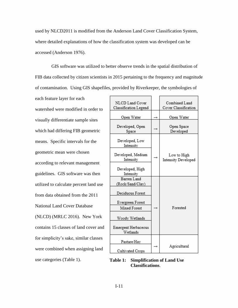


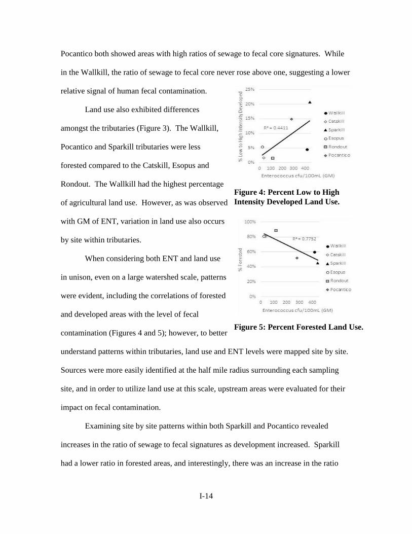


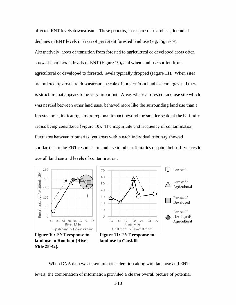
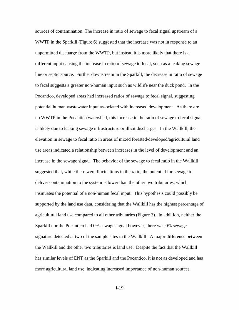


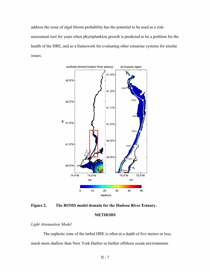
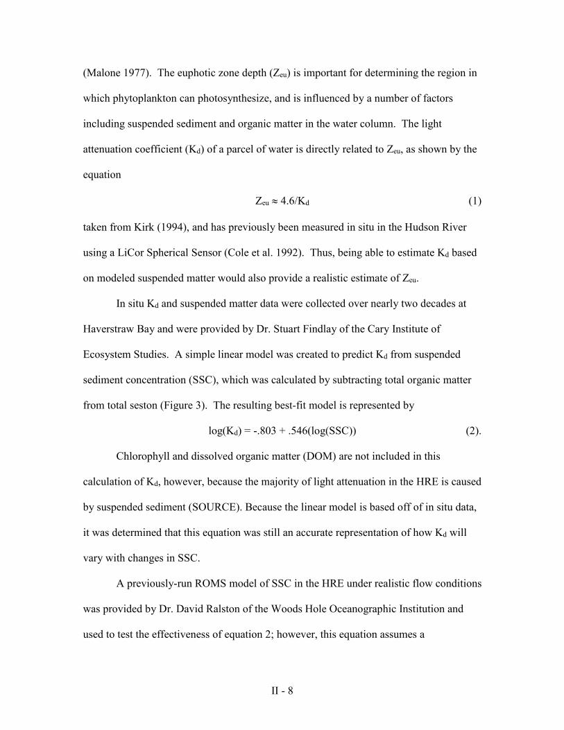
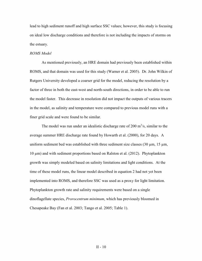

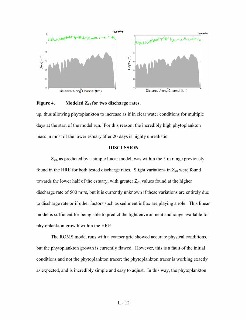
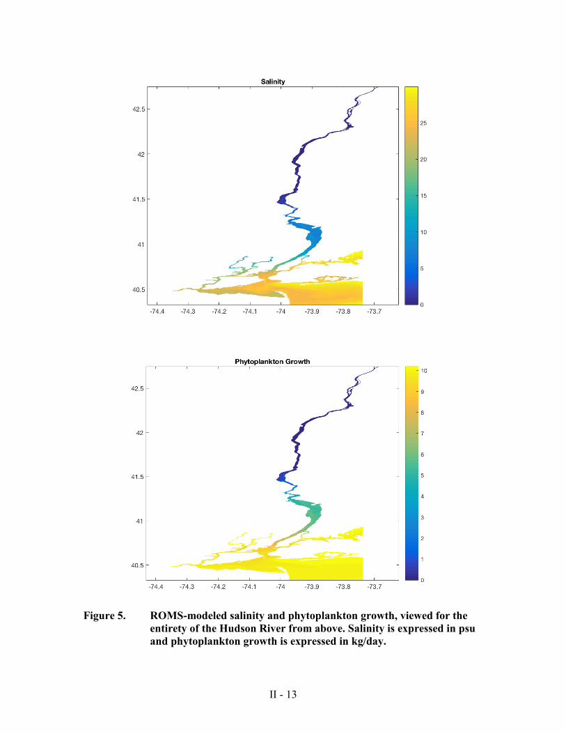


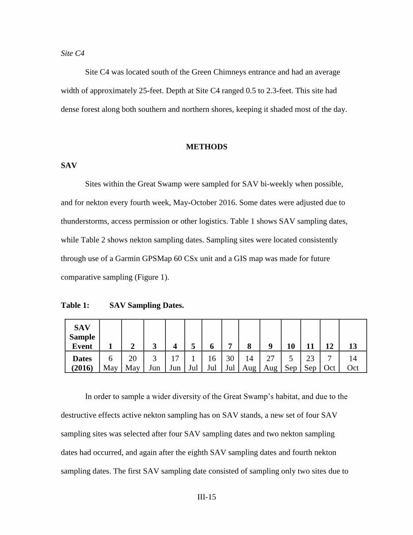


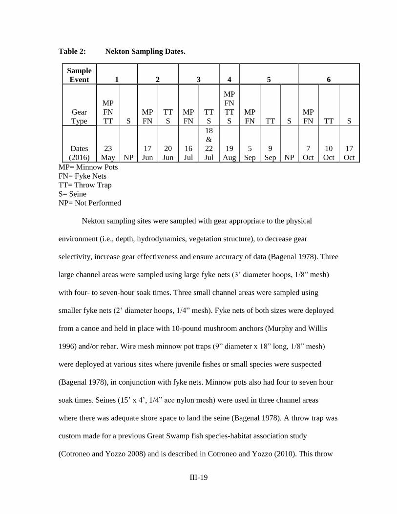
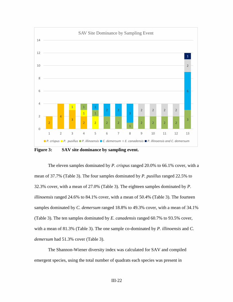


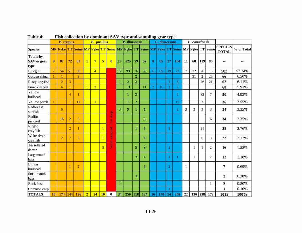

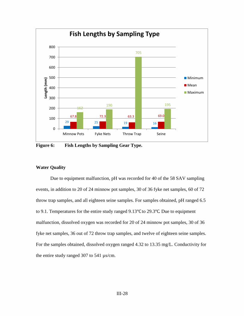


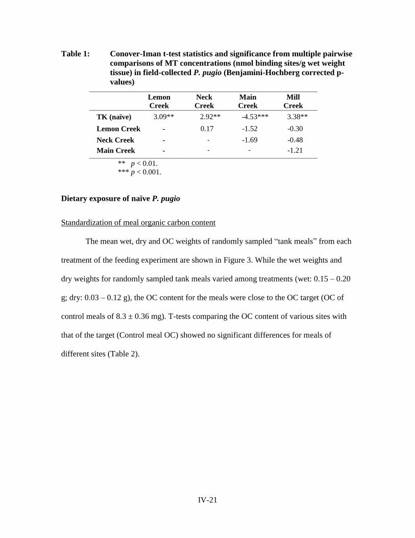


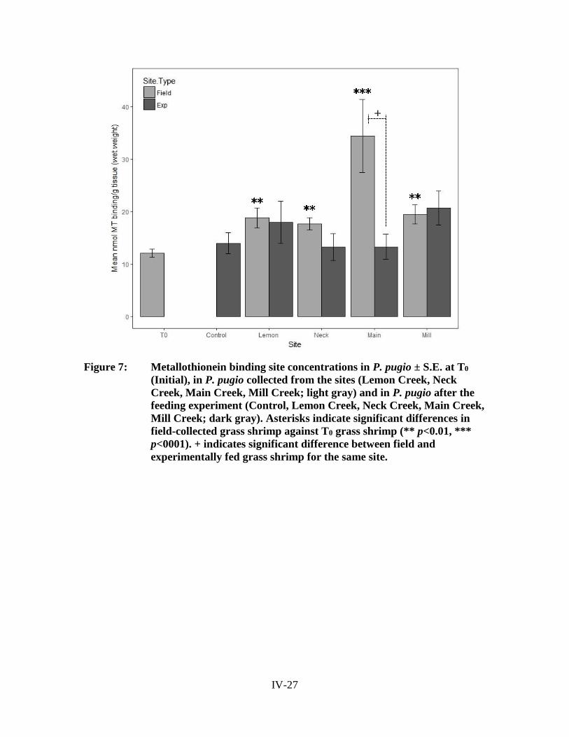


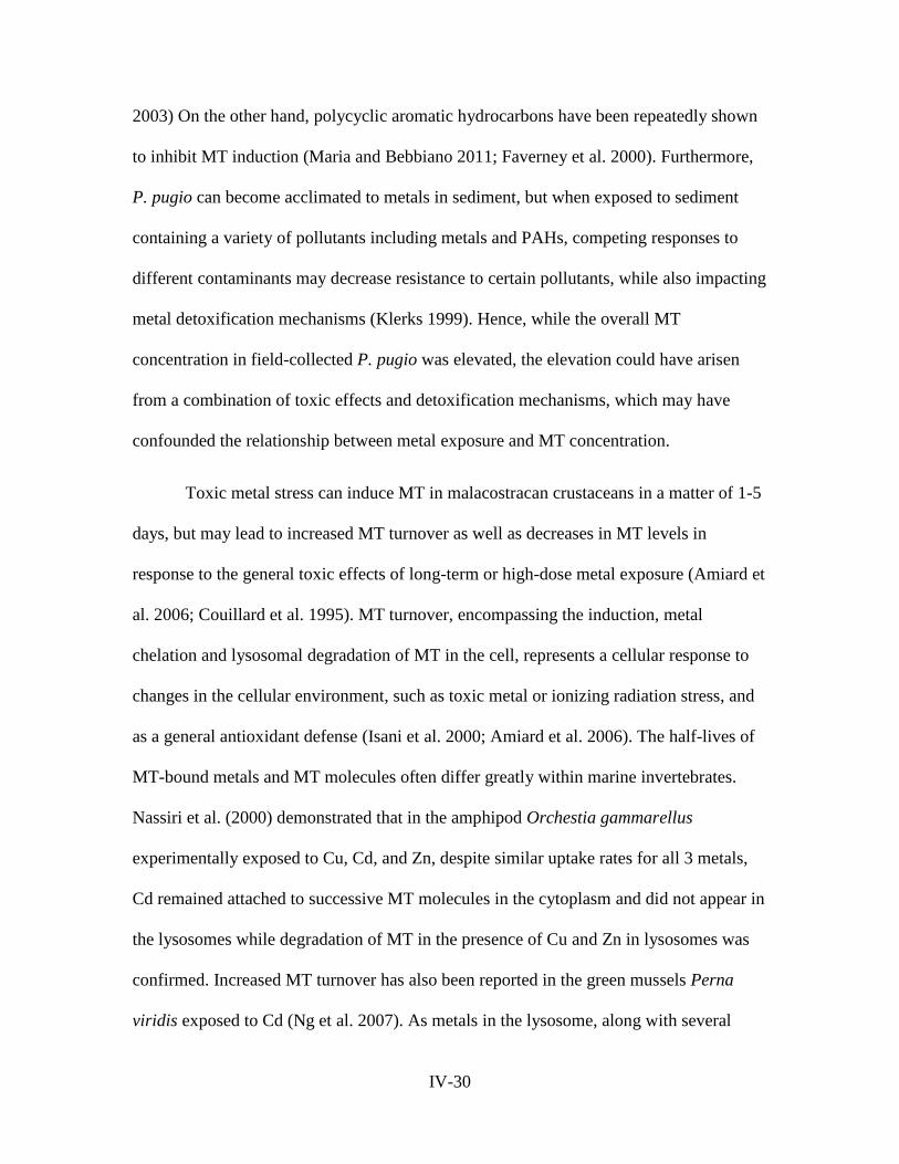


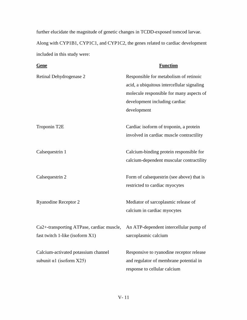

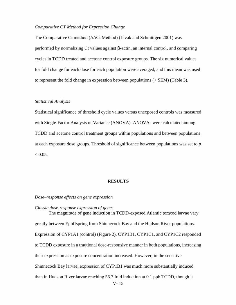


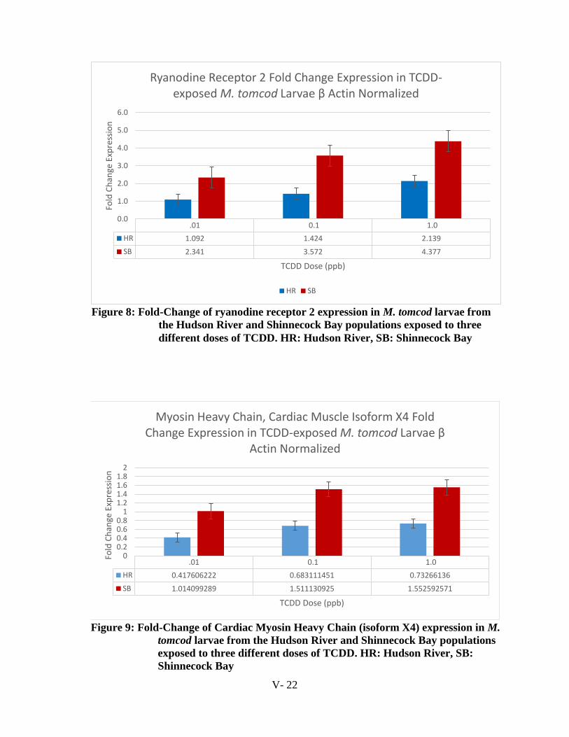
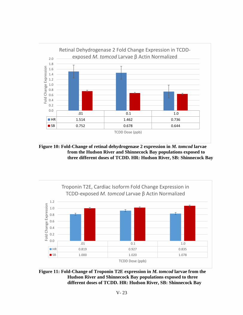


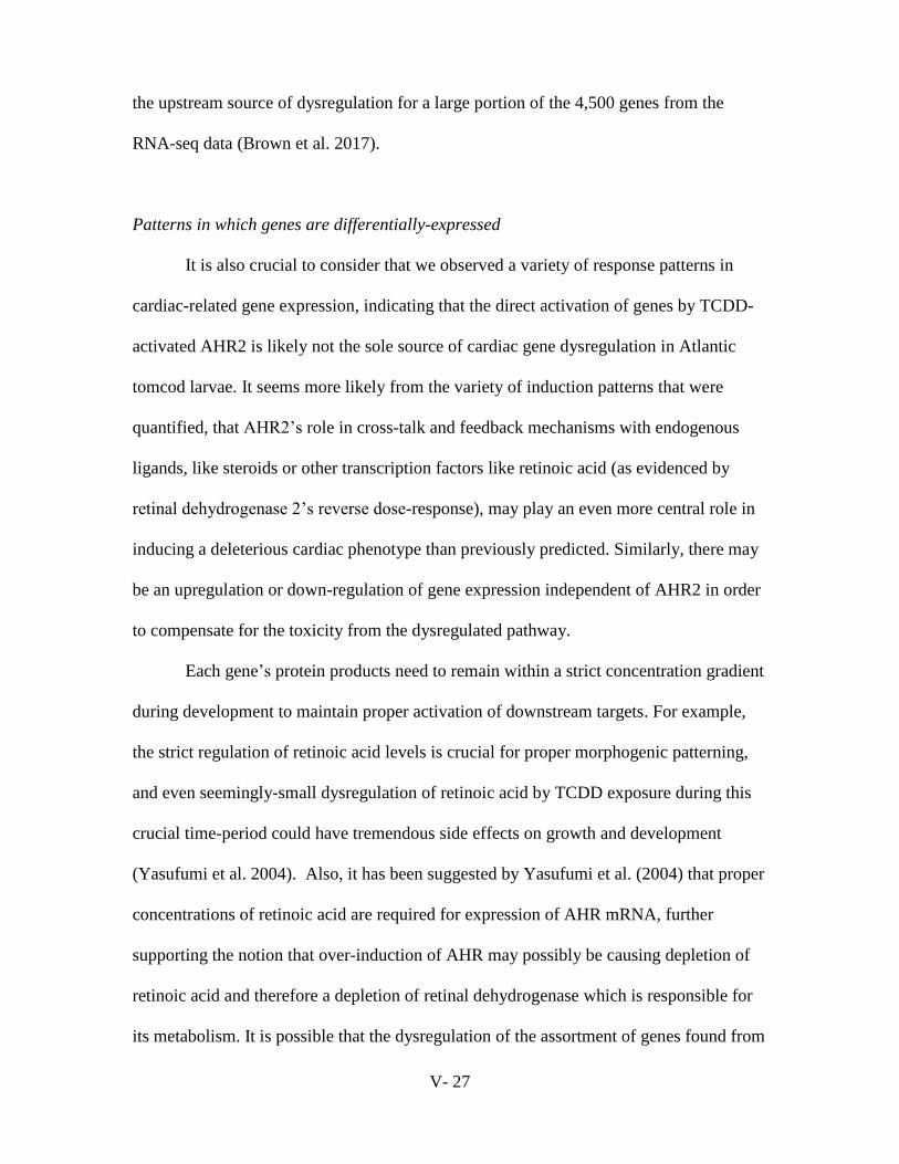


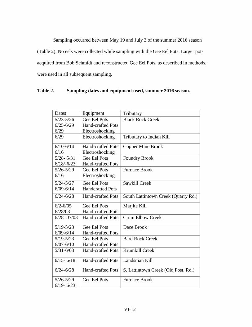


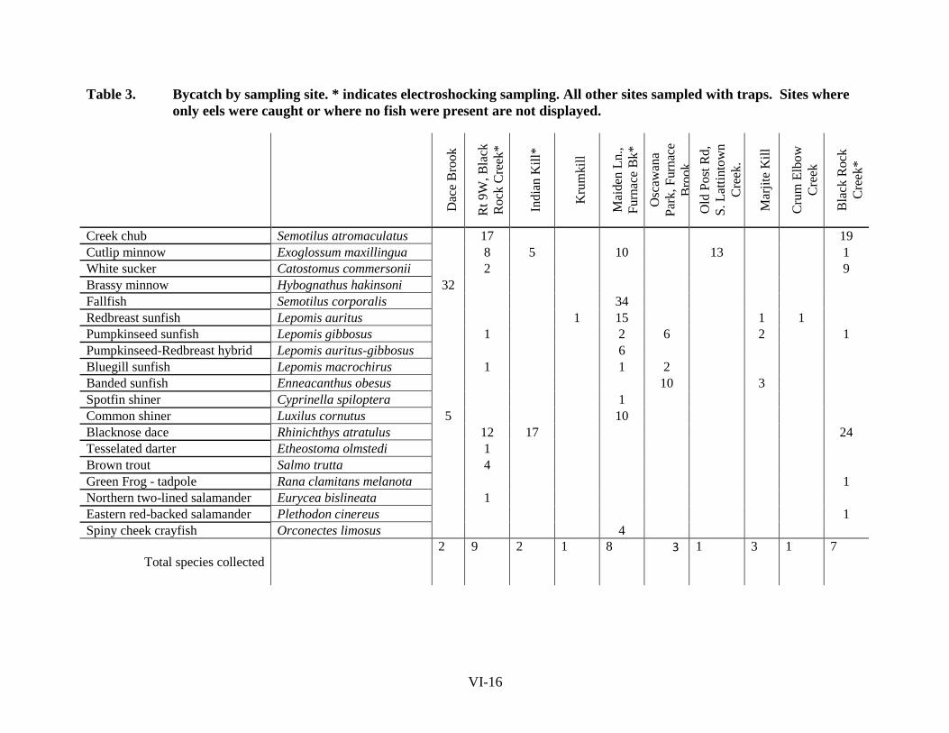
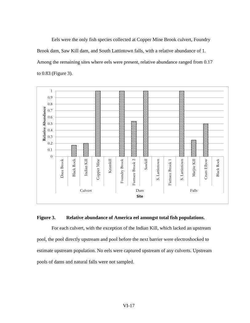

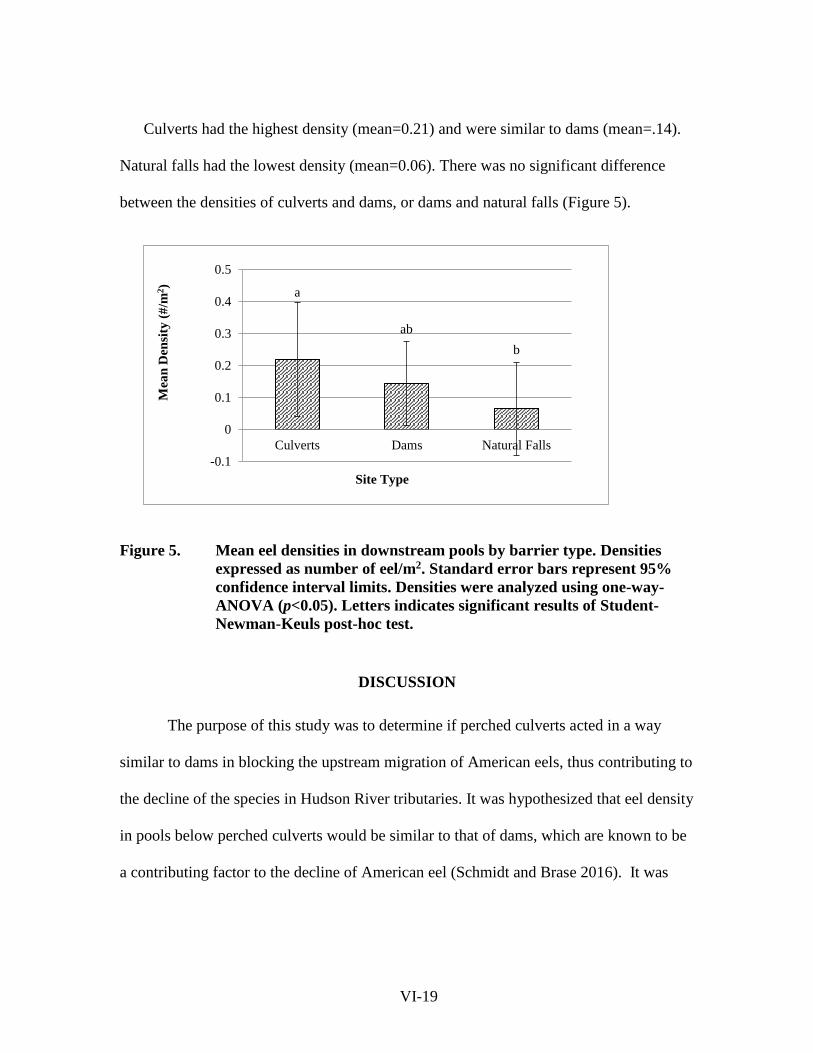


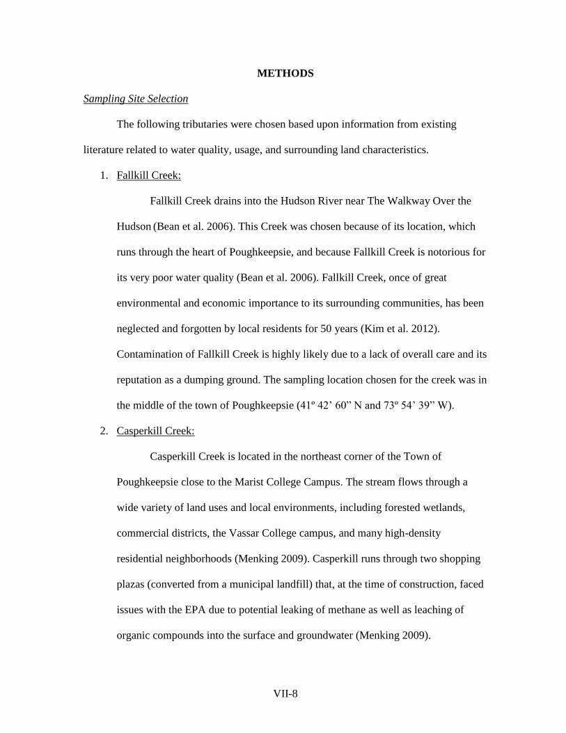
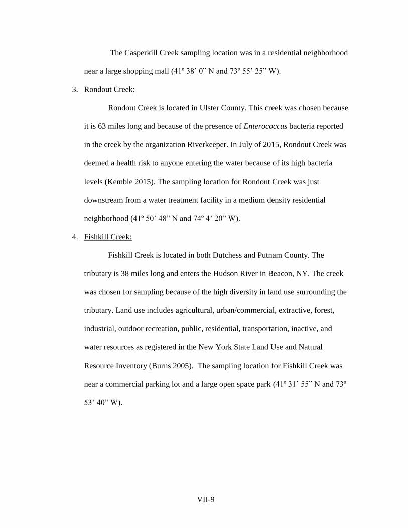


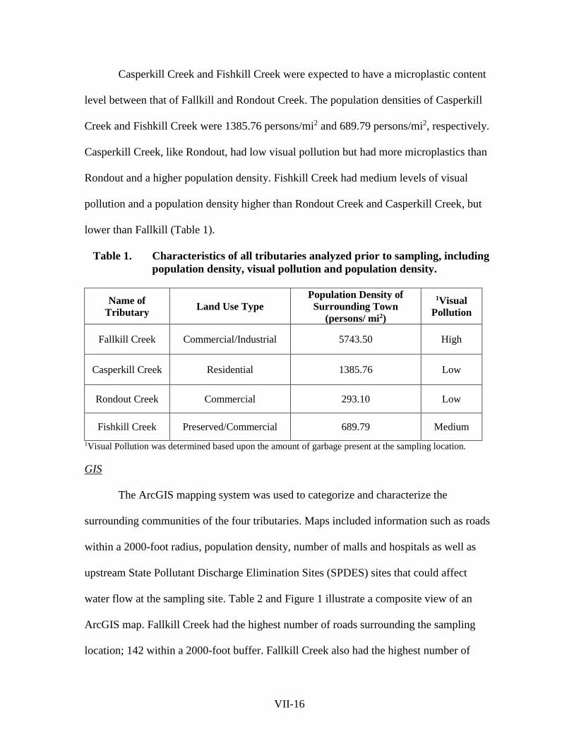
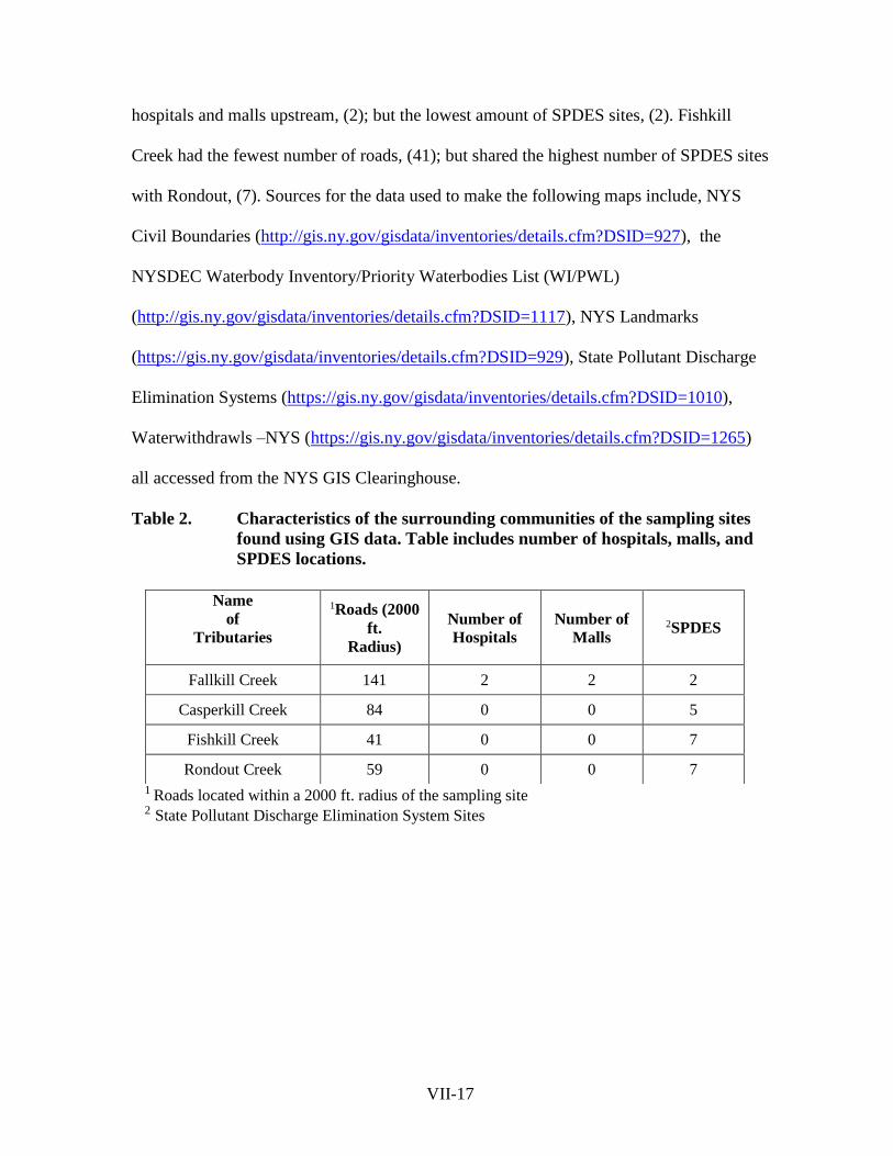


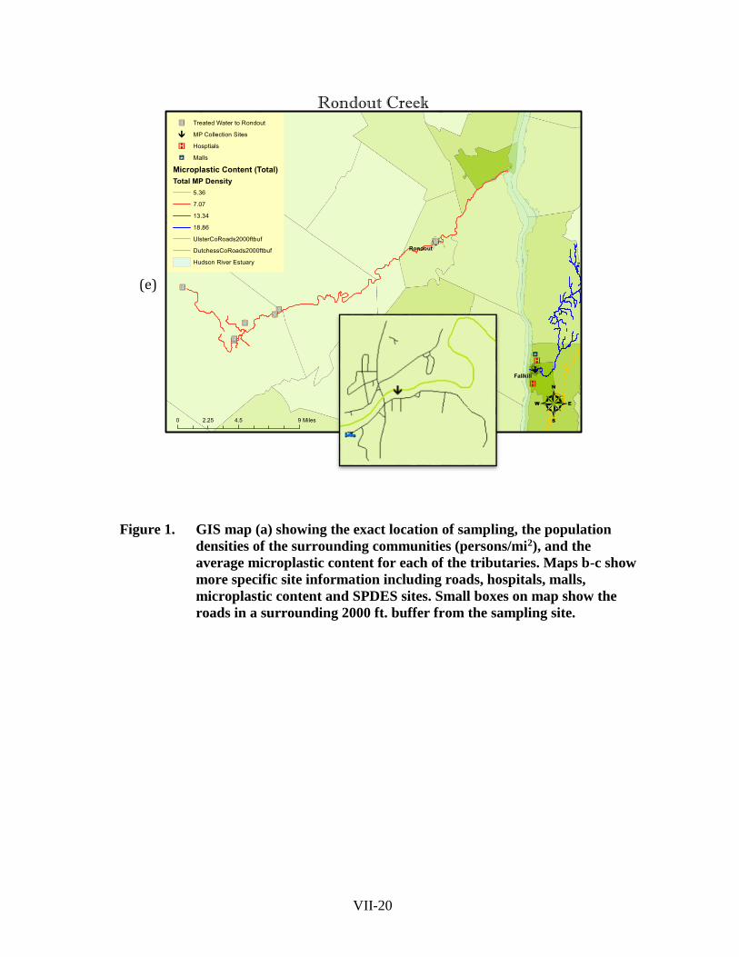


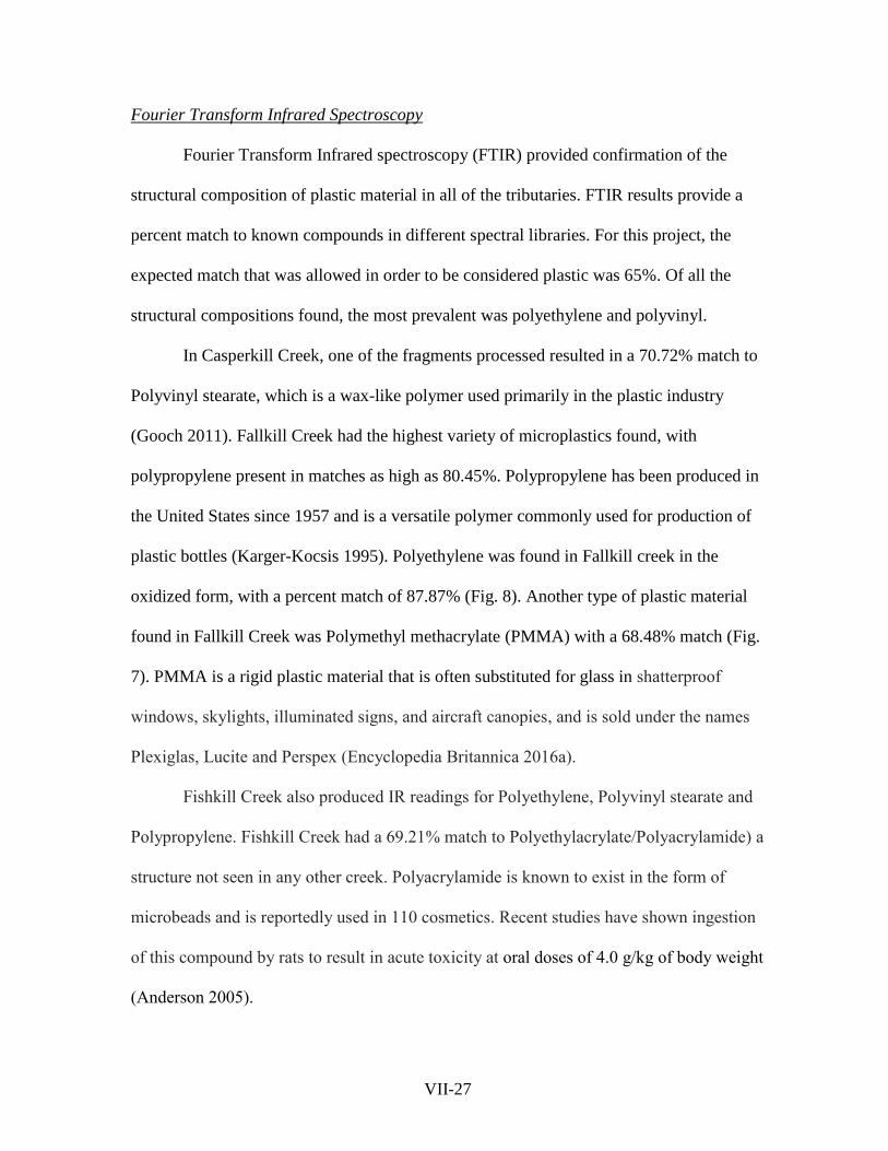

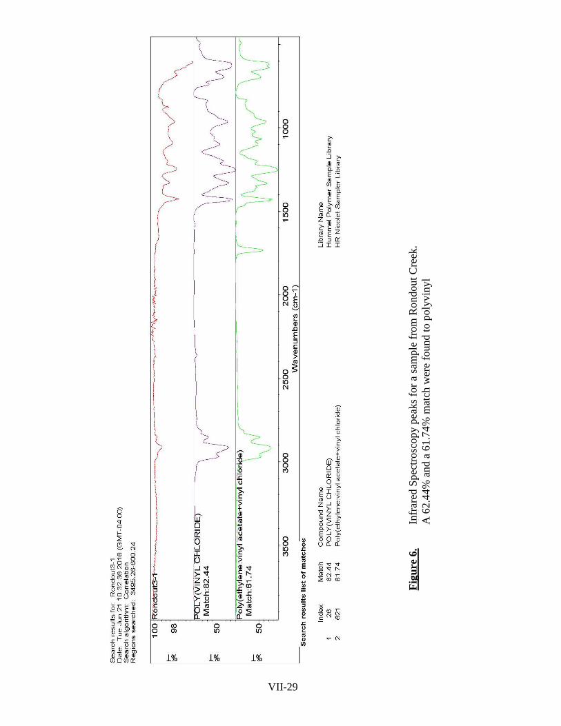
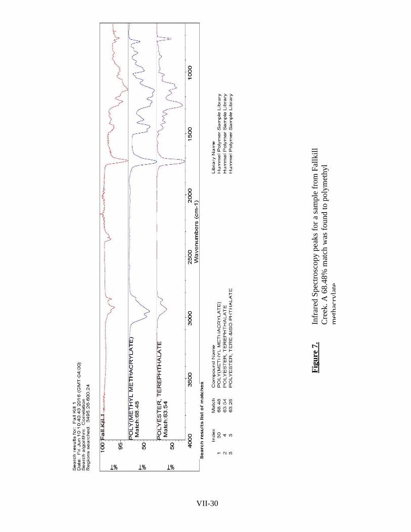
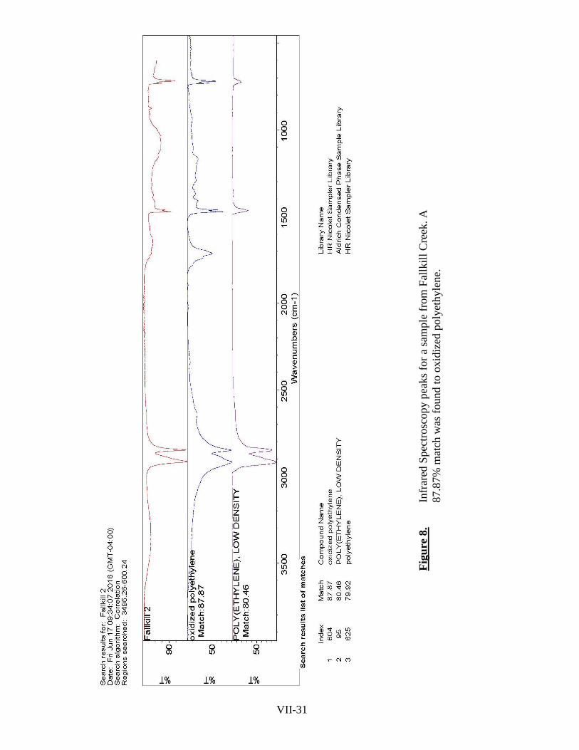


![5334 Problems - Polgar [SOLUTIONS]](https://static.documents.pub/doc/80x56/563db98e550346aa9a9e7977/5334-problems-polgar-solutions.jpg)


