Research ArticleRadial Basis Function Neural Network with ParticleSwarm Optimization Algorithms for Regional LogisticsDemand Prediction
Zhineng Hu Yixin Zhang and Liming Yao
Uncertainty Decision-Making Laboratory Sichuan University Chengdu 610064 China
Correspondence should be addressed to Liming Yao lmyaoscueducn
Received 26 June 2014 Revised 8 September 2014 Accepted 4 November 2014 Published 26 November 2014
Academic Editor Zhigang Jiang
Copyright copy 2014 Zhineng Hu et al This is an open access article distributed under the Creative Commons Attribution Licensewhich permits unrestricted use distribution and reproduction in any medium provided the original work is properly cited
Regional logistics prediction is the key step in regional logistics planning and logistics resources rationalization Since regionaleconomy is the inherent and determinative factor of regional logistics demand it is feasible to forecast regional logistics demandby investigating economic indicators which can accelerate the harmonious development of regional logistics industry and regionaleconomy In this paper the PSO-RBFNN model a radial basis function neural network (RBFNN) combined with particle swarmoptimization (PSO) algorithm is studied The PSO-RBFNN model is trained by indicators data in a region to predict the regionallogistics demand And the corresponding results indicate the modelrsquos applicability and potential advantages
1 Introduction
With the rapid economic development and the continuousadvancement of information and technology modern logis-tics industry is developing fast on a global scale Thereforelogistics industry is considered to be the foundation as well asthe basic industry of national economic development Mean-while its level of development becomes an essential symbolof measuring a countryrsquos modernization and comprehensiveeconomic strength
Regional logistics demand prediction system is a cru-cial part of regional logistics system planning and logisticsrational allocation process of resources This is because theregional logistics demand prediction system provides thenecessary basis for decisionmaking of the government It alsoprovides support for the construction of logistics infrastruc-ture Scholars at home and around theworld establishedmorepredictive models for macrologistics needs for examplethe space-time multinomial probity model of forecastingfreight transportation [1] nonlinear air services demandmodel based on time series [2] stepwise linear regressionmethod for cargo forecasting [3] logistics demand analysismodel combining input-output and spatial price [4] routecomparison model and gravity model [5] grey prediction
model fuzzy forecast and neural network prediction modeland so forth [6ndash8] Yet few scholars combined regional eco-nomic development with regional logistics demand forecastsclosely togetherThe vast majority of the literature focused onusing historical data of logistics needs for logistics demandforecasting rather than utilizing economic data to forecastdemand for logistics
Many domestic and foreign scholars have conductedresearches on the prediction of regional logistics demand Itis basically divided into two categories time series predictionmethod and causality predictionmethod Time series predic-tion method is a kind of approach based on the evolutionrules of the predicted object which are found out from thehistorical data of the time series Commonly used modelsinclude moving average exponential smoothing and greymodel Causality predictionmethod is to infer the developingtrend of things by establishing the appropriate causality fore-casting model based on the relationship between variablesof prediction object and variables of its related things foundout from historical data and using the causal relationship ofthings development Commonly used models include elasticcoefficient method linear regression model and artificialneural network model Commonly used prediction methodsand the applicable situation are shown in Table 1
Hindawi Publishing CorporationDiscrete Dynamics in Nature and SocietyVolume 2014 Article ID 414058 13 pageshttpdxdoiorg1011552014414058
2 Discrete Dynamics in Nature and Society
Table 1 Common forecasting methods
Forecasting methods The applicable situationMoving average [24] Suitable for spot predictionExponentialsmoothing [25]
Repeated prediction with or without achange in seasons
Grey model [6] Development of time series showingexponential trend
Elastic coefficientmethod [26]
Two factors between119883 and 119884 have anexponential relationship
Linear regressionmodel [3]
A linear relationship betweenindependent variables and dependentvariables
Artificial neuralnetwork model [7]
Being able to make prediction ofnonlinear corresponding relationship
Time series forecasting method does not consider theinfluence of other economic development indicators It dis-regards that the regional logistics demand is of derivationHence there are often serious prediction errors On the otherhand compared with the macrologistics regional logisticsdemand prediction has its own characteristics there existsa high degree of nonlinearity between logistics demand andthe impact of logistics demand indicators as well as greatervolatility than macrologistics Due to these features the tra-ditional time series forecastingmethods (such as greymodel)and linear prediction methods (such as linear regressionmodel) do notwork effectively Consequently artificial neuralnetwork (ANN) model is more suitable Furthermore it isexactly the complexity and nonlinearity of regional logisticsdemand system that make a single predictionmodel functionnot well [9ndash12] Therefore it is necessary to use a combinedmodel
In this paper a regional logistics demandprediction indexsystem with economic indicators and logistics indicatorsand a regional logistics demand prediction model based onradial basis function neural network (RBFNN) combinedwith particle swarm optimization (PSO) algorithm will bebuilt The PSO-RBFNNmodel will be trained with processeddata from Sichuan province and will be applied to predictthe regional logistics demand in the very area as well Theprediction result will be evaluated and compared with abackpropagation (BP) neural network and regular RBFNNEventually the results and conclusions drawn from the PSO-RBFNNpredictionmodel will be discussed and summarized
2 Problem Description
21 Problem Background In order to enhance the investmentenvironment to increase the attraction of foreign invest-ment to solve the employment pressure and to improvethe comprehensive competitiveness of urban areas multipleregions in China have adopted a variety of planning policiesto encourage the development of logistics and construction oflogistics infrastructure Nonetheless Chinarsquos logistics startedlate and the related policies strategies and planning arenot mature Plannersrsquo understanding of the development ofmodern logistics concept and mode of operation is still not
unified especially in the field of logistics demand and soon When formulating logistics development policies andstudying the feasibility of logistics infrastructure scholarsascertain that the lack of quantitative data about logisticsdemand results in numerous problems in the planningprocess for instance the imbalance between actual supplycapacity of logistics and logistics demand repeated construc-tion and sedimentation of money caused by tremendouswaste of resources and false prosperity of logistics industryOverall predicting regional logistics demand is critical for thesustainable development of regional logistics industry
Therefore the quantitative prediction of the scale anddevelopment trends of logistics demand is essential To beginwith this kind of predictions can purposefully guide socialinvestment into the field of logistics Various types of logisticsinfrastructure can be rationally planned and constructedlogistics supply system and network layout can be improvedMoreover the predictions continuously provide the basis forthe supply to meet the demand so as to maintain a relativebalance between supply and demand for logistics services andto make the regional logistics maintain high efficiency
22 Related Concepts of Regional Logistics Demand Cur-rently there is no uniform view for the definition of regionallogistics Dong [13] holds that regional logistics is a systemaiming at optimizing the socioeconomic strategies throughthe planning and construction of a certain region Mean-while it also refers to activities associated with logistics oper-ation and control In accordance with the systems definedby systems engineering the regional logistics system canbe defined as follows in a certain economic geographicarea it is an organic whole with specific operating lawand function formed by interrelated interdependent andinteracting elements of all logistics at different spatial scalesThe regional logistics system is illustrated in Figure 1
Compared with the national logistics systems and enter-prise logistics system the regional logistics system is anorganic integrated logistics system within the range of theeconomic region The basic structural unit of the regionallogistics system is a microenterprise supply sales logisticsand so on Meanwhile it is a vital part of the nationallogistics international logistics and other macrologisticssystems The regional logistics system which is mesolevelbecomes the convergence of the microscopic and macro-scopic logistics systems Its purpose is to apply the logisticschain management solutions to address a variety of logisticalproblems beyond a single enterprise so as to achieve logisticsrationalization in a region or in a wider range of areas [14ndash16]as is indicated in Figure 2
Logistics demand prediction is based on the relation-ship between past and current logistics market demandinformation and factors affecting the changes in the logis-tics market demand It uses sound judgment experiencetechnical methods and predictive models on the basis ofhistorical data and statistical information to derive someregularity trends and intrinsic link trends among the factorswhich predicts indicators reflecting market demand trendsLogistics demand prediction is preestimates and predictions
Discrete Dynamics in Nature and Society 3
TargetKeep balance
Dem
and
Dem
and
Primary industry
Secondary industry
Tertiary industry
Logistics infrastructure
Logistics park
Logistics enterprises
Figure 1 The regional logistics system
Urbandistribution
centers
Manufacturers
Distributors
Consumer
Warehousing
Machining
Package
Handling
Regionallogisticscenter
Airport
Port
Railway freightstation t
RTS highway t
The international
City
Region
The domestic
Figure 2 Internal structure of regional logistics system
of the cargo traffic source flow velocity and other goodsconstituting in the area which have not occurred or is not yetclear so as to meet the scale of regional logistics demand andhierarchy of needs Finally it provides decision-making basisfor the regional logistics planning
3 Methodologies
Beforemodeling we select suitable regional logistics demandprediction indicators thereby keeping accuracy and reliabil-ity of regional logistics demand prediction
4 Discrete Dynamics in Nature and Society
31 Selecting the Regional Logistics Demand Indicators Theregional logistics demand scale indicator is the most impor-tant indicator in regional logistics demand indicators Itreflects the development of the logistics industry and thesupply of logistics services in the region namely the sizeand level of total demand for logistics It is also the mostsignificant data the government and corporate decision-makers should first master Generally scale indicators ofregional logistics demand can be set from several differentangles as demonstrated in Table 2
According to the logistic current situation and the prin-ciple of regional logistic prediction indicators we select totalfreight traffic (TFT 119910
1 10 000 tons) and freight turnover (FT
1199102 100 million ton-km) as the prediction targetsRegional economic indicators are the economic indica-
tors utilized in the prediction and have tremendous impactson regional logistics demand The total regional economyregional economic structure and distribution are majoreconomic factors impacting regional logistics demand Inaddition intraregional trade regional income per capita andconsumption level are also important influencing factorsHence when setting regional economic indicators we selectas many related indicators as we can tomake predictionmoreeffectiveMeanwhile we have to consider that indicatorsrsquo datashould be relatively easy to obtain from the regional statisticalyearbook Regional economic indicators are set using themeasures illustrated in Table 3
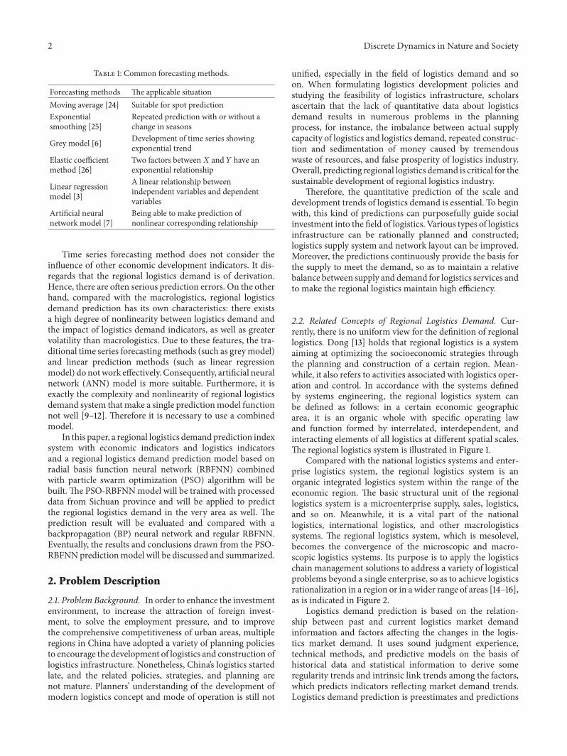
32 Building Regional Logistics Demand Prediction IndexSystem Combined with the previous analysis and takinginto account the availability of statistical data limits in thisresearch we select total freight traffic (TFT 119910
1 10 000 tons)
and freight turnover (FT 1199102 100 million ton-km) to measure
the scale of regional logistics demand Likewise we selectgross domestic product (GDP 119909
1 billion yuan) primary
industry output value (PIO 1199092 billion yuan) secondary
industry output value (SIO1199093 billion yuan) tertiary industry
output value (TIO 1199094 billion yuan) regional retail sales
(RRS 1199095 million yuan) total import and export (TIE 119909
6
million dollar) and per capita consumption (PCC 1199097 yuan
per person) as economic indicators to predict the regionallogistics demand These indicators of input and output willbe utilized to train the PSO-RBFNN and predict the regionallogistics demandThe index system predicting regional logis-tics demand is exhibited in Figure 3
33The Radial Basis FunctionNeural Network (RBFNN) Theartificial neural network (ANN) is a nonlinear informationprocessing system which imitates human brain structure andfunction According to the potential law ANN is able toextrapolate new output by using new input Hence ANNhas the ability to adapt to the changing environment andto achieve real value mapping of any complex functionsANN is widely utilized to resolve problems such as patternrecognition forecasting andprediction optimization controland intelligent decision-making The feedforward neuralnetworks are one of the most widely used ANNs Backprop-agation (BP) network radial basis function neural network
Table 2 Regional logistics demand indicators
Indicatorspecies
Classificationstandards Setting indicators
Indicators oflogisticsdemand scale
Freight scale Volume of freight trafficand freight turnover
Logistics costsTotal logistics costs and theproportion of logistics costsin GDP
Investment infixed assets
Total investment inlogistics fixed assets
Industrypersonnel
The proportion of thenumber of employees intotal employment or totalpopulation
Indicators of economic scale Gross domestic product (GDP)and GDP per capita
Indicators of industrialstructure
Primary industry output valuesecondary industry output valueand tertiary industry outputvalue
Indicators of trade Regional retail sales and totalvolume of regional foreign trade
Indicators of householdconsumption level
Consumption level per capitaand income per capita
(RBFNN) and group method of data handling (GMDH)network are the typical feedforward neural networks
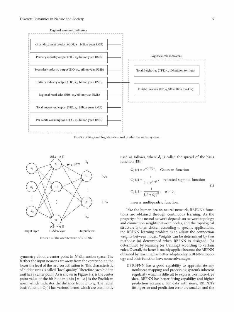
The radial basis function neural network (RBFNN) wasproposed by Moody and Darken [17] It is a commonlyused FNN with only one hidden layer A RBFNN consistsof three layers the input layer the hidden layer and theoutput layer The transformation from the input layer to thehidden layer is nonlinear The output layer is linear andgives a summation at the output units The architecture ofRBFNN is illustrated in Figure 4 where 119899 input units ℎhidden units and 119898 output units are in the RBFNN x =
[1199091 1199092 119909
119899]119879isin R119899 is the input vector W = Rℎtimes119898 is the
output weight matrix 1198871 119887
119898are the output units migra-
tion y = [1199101 1199102 119910
119898]119879 is the output vector Φ
119894(119909 minus 119888
119894)
is 119894th hidden unitrsquos activation function sum in the output unitindicates that the output layer neurons use linear activationfunction As a result the 119896th output can be represented as119910119896= sumℎ
119894=1119908119894Φ119894(119909 minus 119888
119894) where 119908
119894denotes the connection
weight with which decision makers endow the radial basisfunction
The essential feature of the RBFNN is that it utilizes thedistance (Euclidean distance) function as the basis functionand the radial basis function (such as Gaussian function)as activation functions The radial basis function is a radial
Discrete Dynamics in Nature and Society 5
Regional economic indicators
Logistics scale indicators
Gross document product (GDP x1 billion yuan RMB)
Primary industry output (PIO x2 billion yuan RMB)
Secondary industry output (SIO x3 billion yuan RMB)
Tertiary industry output (TIO x4 billion yuan RMB)
Regional retail sales (RRS x5 billion yuan RMB)
Total import and export (TIE x6 billion yuan RMB)
Per capita consumption (PCC x7 billion yuan RMB)
Freight turnover (FTy2100million ton-km)
Total freight trac (TFTy2 100million ton-km)
Figure 3 Regional logistics demand prediction index system
Input layer Hidden layer Output layer
W isin Rhtimesm
x1
x2
xn
c1
c2
ch
Σ
Σ
b1
bm
y1
ym
120601(x minus c1)
120601(x minus ch)
Figure 4 The architecture of RBFNN
symmetry about a center point in 119873-dimension space Thefarther the input neurons are away from the center point thelower the level of the neuron activation is This characteristicof hidden units is called ldquolocal qualityrdquoTherefore each hiddenunit has a center point As is shown in Figure 4 119888
119894is the center
point value of the 119894th hidden unit 119909 minus 119888119894 is the Euclidean
norm which indicates the distance from 119909 to 119888119894 The radial
basis function Φ119894(sdot) has various forms which are commonly
used as follows where 120575119894is called the spread of the basis
function [18]
Φ119894(119905) = 119890
minus(11990521205752
119894) Gaussian function
Φ119894(119905) =
1
1 + 11989011990521205752 reflected sigmoid function
Φ119894(119905) =
1
(1199052 + 1205752
119894)120572 120572 gt 0
inverse multiquadric function
(1)
Like the human brainrsquos neural network RBFNNrsquos func-tions are obtained through continuous learning As theproperty of the neural network depends on network topologyand connection weights between nodes and the topologicalstructure is often chosen according to specific applicationsthe RBFNN learning problem is to adjust the connectionweights between nodes Weights can be determined by twomethods (a) determined when RBFNN is designed (b)determined by learning (or training) according to certainrules Overall the latter ismainly applied because the RBFNNobtained by learning has better adaptability RBFNNrsquos topol-ogy and basis function have some advantages
(1) RBFNN has a good capability to approximate anynonlinear mapping and processing systemrsquos inherentregularity which is difficult to express For noise-freedata RBFNN has better fitting capability and higherprediction accuracy For data with noise RBFNNrsquosfitting error and prediction error are smaller and the
6 Discrete Dynamics in Nature and Society
convergence rate is faster than other neural networkssuch as BP neural network
(2) RBFNN topology can not only improve the learn-ing speed but also avoid the local minimum Inaddition RBFNNrsquos transfer function adopts radialbasis functions particularly the Gaussian functionAs the Gaussian function has a simple representationso even a multivariable input would not add muchcomplexity And it is easy to theoretically analyse
(3) RBFNN has a self-learning self-organizing self-adaptive capability and a fast learning speed RBFNNcan achieve a wide range of data fusion and dataparallel processing at high speed
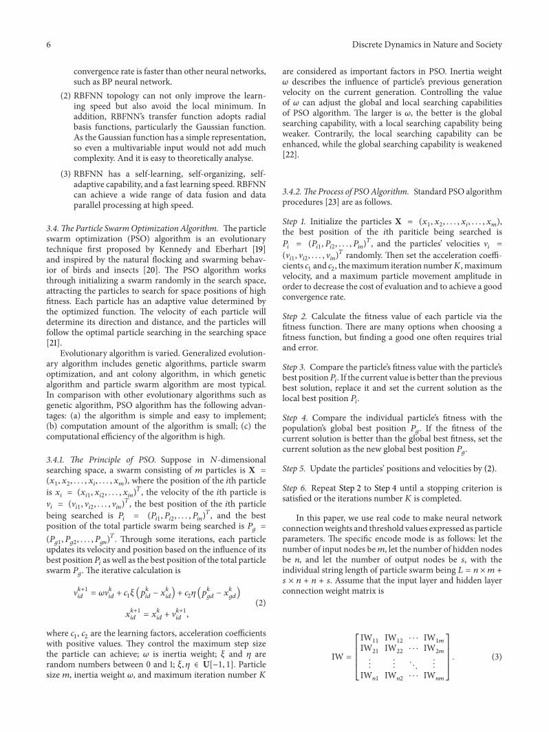
34The Particle SwarmOptimization Algorithm Theparticleswarm optimization (PSO) algorithm is an evolutionarytechnique first proposed by Kennedy and Eberhart [19]and inspired by the natural flocking and swarming behav-ior of birds and insects [20] The PSO algorithm worksthrough initializing a swarm randomly in the search spaceattracting the particles to search for space positions of highfitness Each particle has an adaptive value determined bythe optimized function The velocity of each particle willdetermine its direction and distance and the particles willfollow the optimal particle searching in the searching space[21]
Evolutionary algorithm is varied Generalized evolution-ary algorithm includes genetic algorithms particle swarmoptimization and ant colony algorithm in which geneticalgorithm and particle swarm algorithm are most typicalIn comparison with other evolutionary algorithms such asgenetic algorithm PSO algorithm has the following advan-tages (a) the algorithm is simple and easy to implement(b) computation amount of the algorithm is small (c) thecomputational efficiency of the algorithm is high
341 The Principle of PSO Suppose in 119873-dimensionalsearching space a swarm consisting of 119898 particles is X =
(1199091 1199092 119909
119894 119909
119898) where the position of the 119894th particle
is 119909119894= (1199091198941 1199091198942 119909
119894119899)119879 the velocity of the 119894th particle is
V119894= (V1198941 V1198942 V
119894119899)119879 the best position of the 119894th particle
being searched is 119875119894
= (1198751198941 1198751198942 119875
119894119899)119879 and the best
position of the total particle swarm being searched is 119875119892=
(1198751198921 1198751198922 119875
119892119899)119879 Through some iterations each particle
updates its velocity and position based on the influence of itsbest position119875
119894as well as the best position of the total particle
where 1198881 1198882are the learning factors acceleration coefficients
with positive values They control the maximum step sizethe particle can achieve 120596 is inertia weight 120585 and 120578 arerandom numbers between 0 and 1 120585 120578 isin U[minus1 1] Particlesize 119898 inertia weight 120596 and maximum iteration number 119870
are considered as important factors in PSO Inertia weight120596 describes the influence of particlersquos previous generationvelocity on the current generation Controlling the valueof 120596 can adjust the global and local searching capabilitiesof PSO algorithm The larger is 120596 the better is the globalsearching capability with a local searching capability beingweaker Contrarily the local searching capability can beenhanced while the global searching capability is weakened[22]
342The Process of PSOAlgorithm Standard PSO algorithmprocedures [23] are as follows
Step 1 Initialize the particles X = (1199091 1199092 119909
119894 119909
119898)
the best position of the 119894th pariticle being searched is119875119894
= (1198751198941 1198751198942 119875
119894119899)119879 and the particlesrsquo velocities V
119894=
(V1198941 V1198942 V
119894119899)119879 randomly Then set the acceleration coeffi-
cients 1198881and 1198882 themaximum iteration number119870 maximum
velocity and a maximum particle movement amplitude inorder to decrease the cost of evaluation and to achieve a goodconvergence rate
Step 2 Calculate the fitness value of each particle via thefitness function There are many options when choosing afitness function but finding a good one often requires trialand error
Step 3 Compare the particlersquos fitness value with the particlersquosbest position119875
119894 If the current value is better than the previous
best solution replace it and set the current solution as thelocal best position 119875
119894
Step 4 Compare the individual particlersquos fitness with thepopulationrsquos global best position 119875
119892 If the fitness of the
current solution is better than the global best fitness set thecurrent solution as the new global best position 119875
119892
Step 5 Update the particlesrsquo positions and velocities by (2)
Step 6 Repeat Step 2 to Step 4 until a stopping criterion issatisfied or the iterations number 119870 is completed
In this paper we use real code to make neural networkconnectionweights and threshold values expressed as particleparameters The specific encode mode is as follows let thenumber of input nodes be119898 let the number of hidden nodesbe 119899 and let the number of output nodes be 119904 with theindividual string length of particle swarm being 119871 = 119899 times 119898 +
119904 times 119899 + 119899 + 119904 Assume that the input layer and hidden layerconnection weight matrix is
IW =
[[[[
[
IW11
IW12
sdot sdot sdot IW1119898
IW21
IW22
sdot sdot sdot IW2119898
d
IW1198991
IW1198992
sdot sdot sdot IW119899119898
]]]]
]
(3)
Discrete Dynamics in Nature and Society 7
The threshold vector from the input layer to hidden layeris 1198611= [11988711 11988712 119887
1119899]119879 then assume that the hidden layer
and output layer connection weight matrix is
LW =
[[[[
[
LW11
LW12
sdot sdot sdot LW1119899
LW21
LW22
sdot sdot sdot LW2119899
d
LW1199041
LW1199042
sdot sdot sdot LW119904119899
]]]]
]
(4)
The threshold vector from the hidden layer to output layeris 1198612= [11988721 11988722 119887
2119904]119879 So the particlersquos encoding is 119883 =
[IW11sdot sdot sdot IW
11989911989811988721 11988722 119887
2119904]
35The Combination of PSO and RBF As the PSO algorithmcan easily fall into local optimum it fails to achieve globaloptimum The PSO algorithm is not theoretically rigorousproof of convergence to any type of functionsrsquo global extremepoint hence it may be difficult to obtain satisfactory resultsof complex test functions When the PSO algorithm isrunning if the parameter design of the algorithm or theselection of particles is in error it will lead to a rapiddisappearance of the diversity of particles resulting in analgorithm ldquoprematurerdquo phenomenon further restricting thealgorithm from converging to the global extreme point
Meanwhile the PSO algorithmrsquos convergence speed isslow In practical problems it is necessary to reach theappropriate accuracy within a certain period of time and it isnot worth taking a long time to get feasible solutionThis slowconvergence speed is caused by the PSO using an individualoptimum and the global optimum at each iteration
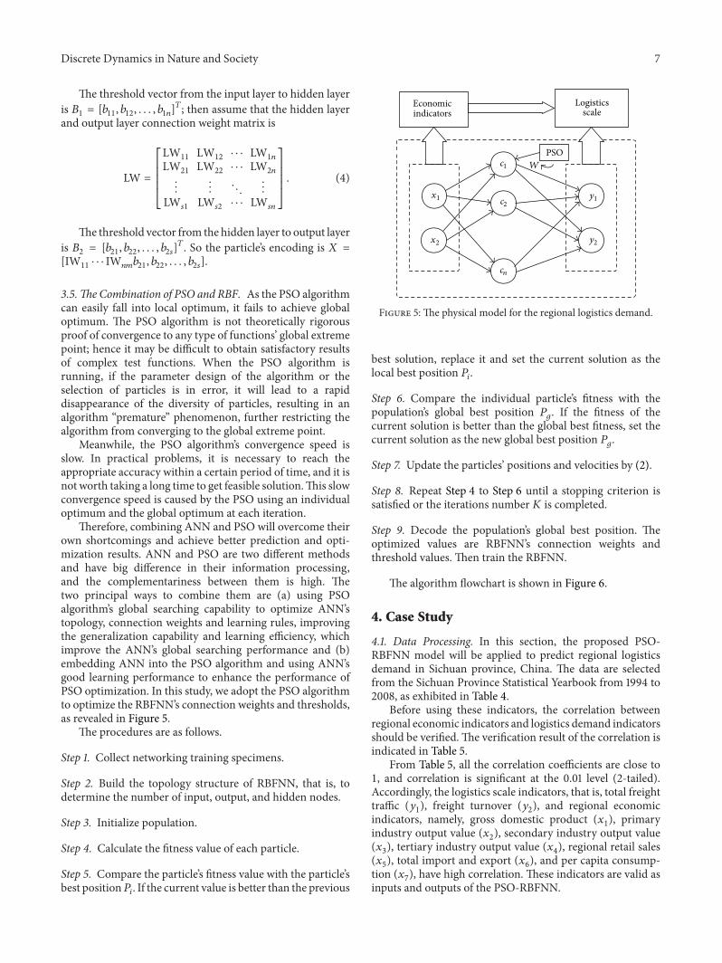
Therefore combining ANN and PSO will overcome theirown shortcomings and achieve better prediction and opti-mization results ANN and PSO are two different methodsand have big difference in their information processingand the complementariness between them is high Thetwo principal ways to combine them are (a) using PSOalgorithmrsquos global searching capability to optimize ANNrsquostopology connection weights and learning rules improvingthe generalization capability and learning efficiency whichimprove the ANNrsquos global searching performance and (b)embedding ANN into the PSO algorithm and using ANNrsquosgood learning performance to enhance the performance ofPSO optimization In this study we adopt the PSO algorithmto optimize the RBFNNrsquos connection weights and thresholdsas revealed in Figure 5
The procedures are as follows
Step 1 Collect networking training specimens
Step 2 Build the topology structure of RBFNN that is todetermine the number of input output and hidden nodes
Step 3 Initialize population
Step 4 Calculate the fitness value of each particle
Step 5 Compare the particlersquos fitness value with the particlersquosbest position119875
119894 If the current value is better than the previous
Economicindicators
Logisticsscale
W
PSO
y1
y2
x1
x2
c1
c2
cn
Figure 5 The physical model for the regional logistics demand
best solution replace it and set the current solution as thelocal best position 119875
119894
Step 6 Compare the individual particlersquos fitness with thepopulationrsquos global best position 119875
119892 If the fitness of the
current solution is better than the global best fitness set thecurrent solution as the new global best position 119875
119892
Step 7 Update the particlesrsquo positions and velocities by (2)
Step 8 Repeat Step 4 to Step 6 until a stopping criterion issatisfied or the iterations number 119870 is completed
Step 9 Decode the populationrsquos global best position Theoptimized values are RBFNNrsquos connection weights andthreshold values Then train the RBFNN
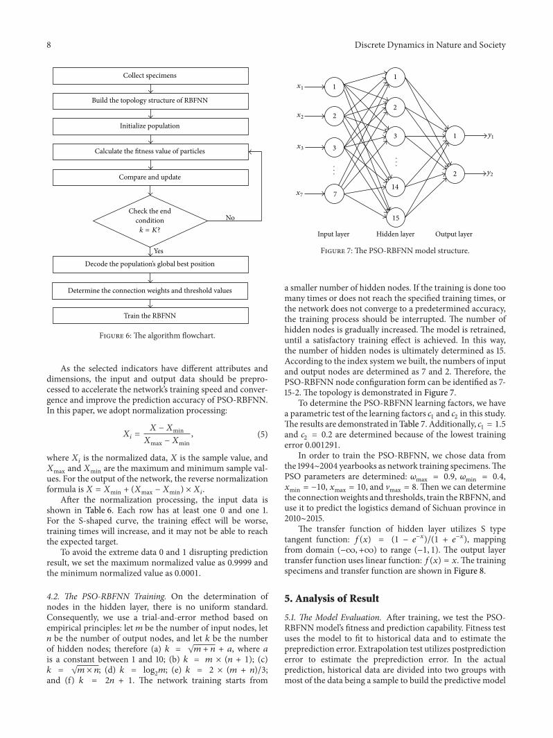
The algorithm flowchart is shown in Figure 6
4 Case Study
41 Data Processing In this section the proposed PSO-RBFNN model will be applied to predict regional logisticsdemand in Sichuan province China The data are selectedfrom the Sichuan Province Statistical Yearbook from 1994 to2008 as exhibited in Table 4
Before using these indicators the correlation betweenregional economic indicators and logistics demand indicatorsshould be verifiedThe verification result of the correlation isindicated in Table 5
From Table 5 all the correlation coefficients are close to1 and correlation is significant at the 001 level (2-tailed)Accordingly the logistics scale indicators that is total freighttraffic (119910
industry output value (1199092) secondary industry output value
(1199093) tertiary industry output value (119909
4) regional retail sales
(1199095) total import and export (119909
6) and per capita consump-
tion (1199097) have high correlation These indicators are valid as
inputs and outputs of the PSO-RBFNN
8 Discrete Dynamics in Nature and Society
Yes
No
Collect specimens
Build the topology structure of RBFNN
Initialize population
Calculate the fitness value of particles
Compare and update
Check the endconditionk = K
Decode the populationrsquos global best position
Determine the connection weights and threshold values
Train the RBFNN
Figure 6 The algorithm flowchart
As the selected indicators have different attributes anddimensions the input and output data should be prepro-cessed to accelerate the networkrsquos training speed and conver-gence and improve the prediction accuracy of PSO-RBFNNIn this paper we adopt normalization processing
119883119894=
119883 minus 119883min119883max minus 119883min
(5)
where 119883119894is the normalized data 119883 is the sample value and
119883max and 119883min are the maximum and minimum sample val-ues For the output of the network the reverse normalizationformula is119883 = 119883min + (119883max minus 119883min) times 119883
119894
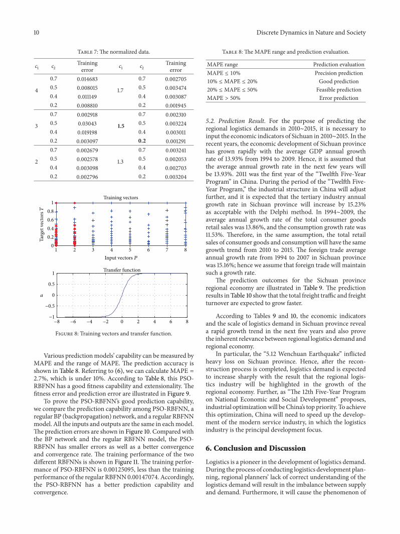
After the normalization processing the input data isshown in Table 6 Each row has at least one 0 and one 1For the S-shaped curve the training effect will be worsetraining times will increase and it may not be able to reachthe expected target
To avoid the extreme data 0 and 1 disrupting predictionresult we set the maximum normalized value as 09999 andthe minimum normalized value as 00001
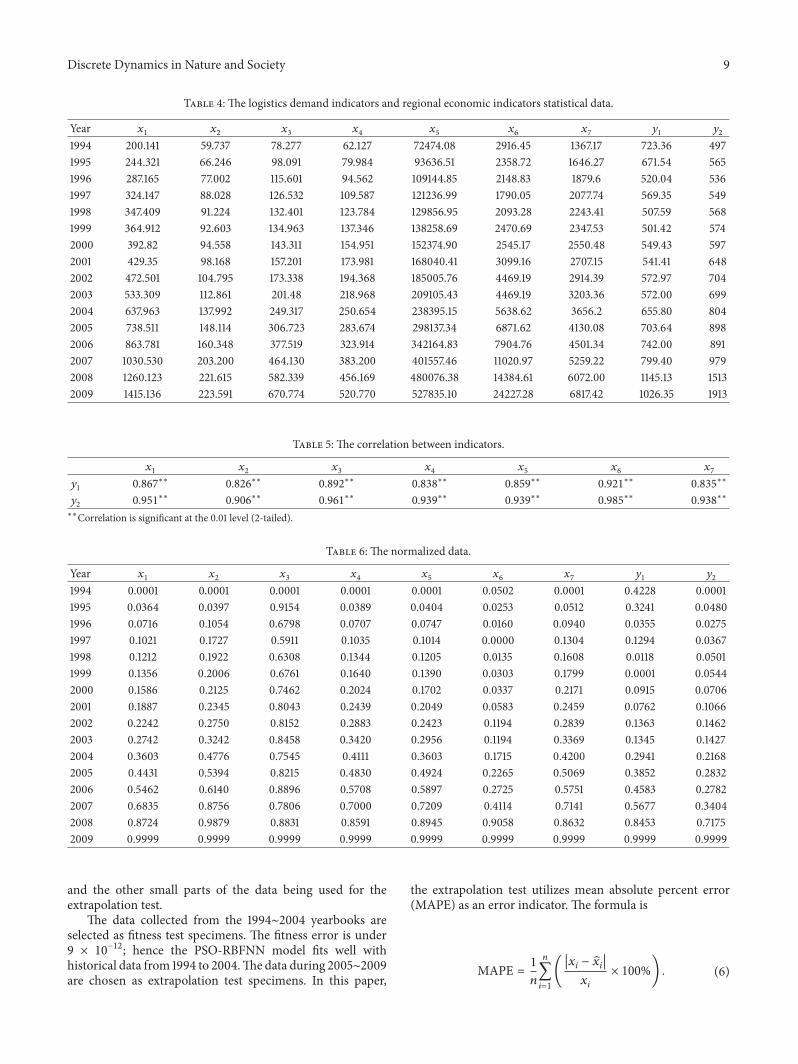
42 The PSO-RBFNN Training On the determination ofnodes in the hidden layer there is no uniform standardConsequently we use a trial-and-error method based onempirical principles let 119898 be the number of input nodes let119899 be the number of output nodes and let 119896 be the numberof hidden nodes therefore (a) 119896 = radic119898 + 119899 + 119886 where 119886
is a constant between 1 and 10 (b) 119896 = 119898 times (119899 + 1) (c)119896 = radic119898 times 119899 (d) 119896 = log
2119898 (e) 119896 = 2 times (119898 + 119899)3
and (f) 119896 = 2119899 + 1 The network training starts from
1
2
3
7
1
2
3
14
15
1
2
Input layer Hidden layer Output layer
x1
x2
x3
x7
y1
y2
Figure 7 The PSO-RBFNNmodel structure
a smaller number of hidden nodes If the training is done toomany times or does not reach the specified training times orthe network does not converge to a predetermined accuracythe training process should be interrupted The number ofhidden nodes is gradually increased The model is retraineduntil a satisfactory training effect is achieved In this waythe number of hidden nodes is ultimately determined as 15According to the index system we built the numbers of inputand output nodes are determined as 7 and 2 Therefore thePSO-RBFNN node configuration form can be identified as 7-15-2 The topology is demonstrated in Figure 7
To determine the PSO-RBFNN learning factors we havea parametric test of the learning factors 119888
1and 1198882in this study
The results are demonstrated in Table 7 Additionally 1198881= 15
and 1198882= 02 are determined because of the lowest training
error 0001291In order to train the PSO-RBFNN we chose data from
the 1994sim2004 yearbooks as network training specimensThePSO parameters are determined 120596max = 09 120596min = 04119909min = minus10 119909max = 10 and Vmax = 8 Then we can determinethe connectionweights and thresholds train the RBFNN anduse it to predict the logistics demand of Sichuan province in2010sim2015
The transfer function of hidden layer utilizes S typetangent function 119891(119909) = (1 minus 119890
minus119909)(1 + 119890
minus119909) mapping
from domain (minusinfin +infin) to range (minus1 1) The output layertransfer function uses linear function 119891(119909) = 119909 The trainingspecimens and transfer function are shown in Figure 8
5 Analysis of Result
51 The Model Evaluation After training we test the PSO-RBFNNmodelrsquos fitness and prediction capability Fitness testuses the model to fit to historical data and to estimate thepreprediction error Extrapolation test utilizes postpredictionerror to estimate the preprediction error In the actualprediction historical data are divided into two groups withmost of the data being a sample to build the predictive model
Discrete Dynamics in Nature and Society 9
Table 4 The logistics demand indicators and regional economic indicators statistical data
and the other small parts of the data being used for theextrapolation test
The data collected from the 1994sim2004 yearbooks areselected as fitness test specimens The fitness error is under9 times 10
minus12 hence the PSO-RBFNN model fits well withhistorical data from 1994 to 2004The data during 2005sim2009are chosen as extrapolation test specimens In this paper
the extrapolation test utilizes mean absolute percent error(MAPE) as an error indicator The formula is
MAPE =1
119899
119899
sum
119894=1
(
1003816100381610038161003816119909119894 minus 119909119894
Various predictionmodelsrsquo capability can bemeasured byMAPE and the range of MAPE The prediction accuracy isshown in Table 8 Referring to (6) we can calculate MAPE =
27 which is under 10 According to Table 8 this PSO-RBFNN has a good fitness capability and extensionality Thefitness error and prediction error are illustrated in Figure 9
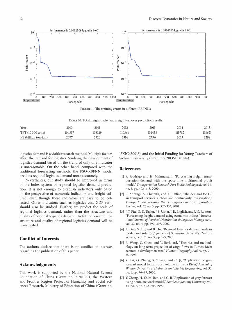
To prove the PSO-RBFNNrsquos good prediction capabilitywe compare the prediction capability among PSO-RBFNN aregular BP (backpropagation) network and a regular RBFNNmodel All the inputs and outputs are the same in eachmodelThe prediction errors are shown in Figure 10 Compared withthe BP network and the regular RBFNN model the PSO-RBFNN has smaller errors as well as a better convergenceand convergence rate The training performance of the twodifferent RBFNNs is shown in Figure 11 The training perfor-mance of PSO-RBFNN is 000125095 less than the trainingperformance of the regular RBFNN 000147074 Accordinglythe PSO-RBFNN has a better prediction capability andconvergence
Table 8 The MAPE range and prediction evaluation
MAPE range Prediction evaluationMAPE le 10 Precision prediction10 le MAPE le 20 Good prediction20 le MAPE le 50 Feasible predictionMAPE gt 50 Error prediction
52 Prediction Result For the purpose of predicting theregional logistics demands in 2010sim2015 it is necessary toinput the economic indicators of Sichuan in 2010sim2015 In therecent years the economic development of Sichuan provincehas grown rapidly with the average GDP annual growthrate of 1393 from 1994 to 2009 Hence it is assumed thatthe average annual growth rate in the next few years willbe 1393 2011 was the first year of the ldquoTwelfth Five-YearProgramrdquo in China During the period of the ldquoTwelfth Five-Year Programrdquo the industrial structure in China will adjustfurther and it is expected that the tertiary industry annualgrowth rate in Sichuan province will increase by 1523as acceptable with the Delphi method In 1994sim2009 theaverage annual growth rate of the total consumer goodsretail sales was 1386 and the consumption growth rate was1153 Therefore in the same assumption the total retailsales of consumer goods and consumption will have the samegrowth trend from 2010 to 2015 The foreign trade averageannual growth rate from 1994 to 2007 in Sichuan provincewas 1516 hence we assume that foreign trade will maintainsuch a growth rate
The prediction outcomes for the Sichuan provinceregional economy are illustrated in Table 9 The predictionresults in Table 10 show that the total freight traffic and freightturnover are expected to grow faster
According to Tables 9 and 10 the economic indicatorsand the scale of logistics demand in Sichuan province reveala rapid growth trend in the next five years and also provethe inherent relevance between regional logistics demand andregional economy
In particular the ldquo512 Wenchuan Earthquakerdquo inflictedheavy loss on Sichuan province Hence after the recon-struction process is completed logistics demand is expectedto increase sharply with the result that the regional logis-tics industry will be highlighted in the growth of theregional economy Further as ldquoThe 12th Five-Year Programon National Economic and Social Developmentrdquo proposesindustrial optimizationwill beChinarsquos top priority To achievethis optimization China will need to speed up the develop-ment of the modern service industry in which the logisticsindustry is the principal development focus
6 Conclusion and Discussion
Logistics is a pioneer in the development of logistics demandDuring the process of conducting logistics development plan-ning regional plannersrsquo lack of correct understanding of thelogistics demand will result in the imbalance between supplyand demand Furthermore it will cause the phenomenon of
Year GDP PIO SIO TIO RRS TIE PCC2010 1612237 244157 774057 600072 60098067 2789982 7588222011 1836791 266614 893241 691451 68426249 3212906 8446172012 2092621 291137 1030778 796745 77908523 3699940 9401122013 2384083 317916 1189491 918072 88704817 4260802 10464042014 2716140 347157 1372642 1057875 100997224 4906683 11647142015 3094447 379088 1583994 1218968 114993071 5650472 1296400
8060402000
minus20minus40minus60
BPPSO-RBFNNRBF
1 2 3 4
Figure 10 The prediction errors in different models
insufficient supply and overinvestment It will also hinderthe development of the logistics industryTherefore studyingthe forecast of regional logistics demand has vital practicalsignificance In this paper based on the theory of regionallogistics demand and its prediction the characteristics andthe main content of regional logistics demand predictionare analyzed the PSO-RBFNN prediction model is builtand an empirical research of logistics demand in Sichuan
province is conducted The principal conclusions are asfollows
(1) By feasibility analysis and empirical research it isproved that a PSO-RBFNN model which introduces a PSOalgorithm to optimizing the RBF neural network connectingweights and thresholds is scientific and practical Combin-ing RBFNN with PSO overcomes their own shortcomingsand achieves better prediction and optimization results (2)Through correlation analysis the strong correlation betweenthe regional economy and regional logistics demand isproven The rapid development of the regional economy willdrive the rapid development of regional logistics (3) In theempirical research we applied the PSO-RBFNN model topredict the regional logistics demand of Sichuan provincefrom 2010 to 2015 After inputting the regional logisticsdemand prediction indicators values into the PSO-RBFNNmodel valid results are calculated in Table 9 suggesting thatthe total freight traffic and freight turnover will increaseby 137 and 588 respectively The PSO-RBFNN modelis utilized to fit well the nonlinear relationship betweenthe regional economy and regional logistics demand (4)Through empirical research it is obvious that using logisticsdemand and regional economic indicators to predict regional
logistics demand is a viable researchmethodMultiple factorsaffect the demand for logistics Studying the development oflogistics demand based on the trend of only one indicatoris unreasonable On the other hand compared with thetraditional forecasting methods the PSO-RBFNN modelpredicts regional logistics demand more accurately
Nevertheless our study should be improved in termsof the index system of regional logistics demand predic-tion It is not enough to establish indicators only basedon the perspective of economic indicators and freight vol-ume even though these indicators are easy to be col-lected Other indicators such as logistics cost GDP ratioshould also be studied Further we predict the scale ofregional logistics demand rather than the structure andquality of regional logistics demand In future research thestructure and quality of regional logistics demand will beinvestigated
Conflict of Interests
The authors declare that there is no conflict of interestsregarding the publication of this paper
Acknowledgments
This work is supported by the National Natural ScienceFoundation of China (Grant no 71301109) the Westernand Frontier Region Project of Humanity and Social Sci-ences Research Ministry of Education of China (Grant no
13XJC630018) and the Initial Funding for Young Teachers ofSichuan University (Grant no 2013SCU11014)
References
[1] R Godrigo and H Mahmassani ldquoForecasting freight trans-portation demand with the space-time multinomial probitmodelrdquo Transportation Research Part B Methodological vol 34no 5 pp 403ndash418 2000
[2] B Adrangi A Chatrath and K Raffiee ldquoThe demand for USair transport services a chaos and nonlinearity investigationrdquoTransportation Research Part E Logistics and TransportationReview vol 37 no 5 pp 337ndash353 2001
[3] J T Fite G D Taylor J S Usher J R English and J N RobertsldquoForecasting freight demand using economic indicesrdquo Interna-tional Journal of Physical Distribution amp Logistics Managementvol 32 no 4 pp 299ndash308 2002
[4] X Guo S Xie and B Hu ldquoRegional logistics demand analysismodel and solutionrdquo Journal of Southeast University (NaturalScience) vol 31 no 3 pp 1ndash5 2001
[5] R Wang C Chen and V Berkhard ldquoTheories and method-ology on long term projection of cargo flows in Tumen Rivereconomic developmen areardquo Human Geography vol 9 pp 21ndash25 1999
[6] Y Lai Q Zheng S Zhang and C Ji ldquoApplication of grayforecast model to transport volume in Jinsha Riverrdquo Journal ofWuhan University of Hydraulic and Electric Engineering vol 33no 1 pp 96ndash99 2000
[7] Y Zhang H Ye M Ren and C Ji ldquoApplication of gray forecastusing neural networkmodelrdquo Southeast Jiaotong University vol34 no 5 pp 602ndash605 1999
Discrete Dynamics in Nature and Society 13
[8] H Niu and Y Yin ldquoFuzzy forecasting on freight demands inrailroad hubrdquo Journal of Lanzhou Railway University vol 17 no3 pp 89ndash94 1998
[9] R Garrido and H Mahmassani ldquoForecasting freight trans-portation demand with the space-time multinomial probitmodelrdquo Transportation Research Part B Methodological vol 34no 5 pp 403ndash418 2000
[10] Q Sun and H Ding ldquoTheory and model establishment forregional logistics demand predictionrdquo Theoretical Discussionno 10 pp 27ndash30 2004
[11] L Chu Z Tian and X Xie ldquoApplication of an combinationforecasting model in logistics demandrdquo Journal of DalianMaritime University vol 30 no 4 pp 43ndash46 2004
[12] J Sun and X Xiang ldquoLogistics demand prediction researchbased on the gray linear regression combination modelrdquo Indus-trial Technology amp Economy vol 26 no 10 pp 146ndash148 2007
[13] Q Dong ldquoRegional logistics information platform and resourceplanningrdquo Traffic and Transportation Engineering no 4 pp 56ndash58 2002
[14] J Xiao ldquoDevelopment of urban centers and modern logisticsindustryrdquo Commodity Storage and Conservation vol 5 pp 7ndash10 2002
[15] X Heng ldquoReflections on the development of logistics enter-prises in Chinardquo Containerization vol 5 pp 21ndash22 2003
[16] Q Zhang ldquoUnited States Japan logisticsrdquo Modern EnterpriseEducation no 4 pp 18ndash19 2003
[17] J Moody and C Darken ldquoFast learning in networks of locally-tuned processing unitsrdquo Neural Computation vol 1 no 2 pp281ndash294 1989
[18] S Haykin Neural Networks and Learning Machines PrenticeHall 2008
[19] J Kennedy and R Eberhart ldquoParticle swarm optimizationrdquoin Proceedings of the IEEE International Conference on NeuralNetworks pp 1942ndash1948 December 1995
[20] E Assareh M A Behrang M R Assari and A GhanbarzadehldquoApplication of PSO (particle swarm optimization) and GA(genetic algorithm) techniques on demand estimation of oil inIranrdquo Energy vol 35 no 12 pp 5223ndash5229 2010
[21] PWang Z-Y HuangM-Y Zhang and X-W Zhao ldquoMechani-cal property prediction of strip model based on PSO-BP neuralnetworkrdquo Journal of Iron and Steel Research International vol15 no 3 pp 87ndash91 2008
[22] Z Ji H Liao and Q Wu Particle Swarm Optimization and ItsApplication Science Press Beijing China 2009
[23] Y Shi and R Eberhart ldquoA modified particle swarm optimizerrdquoin Proceedings of the IEEE International Conference on Evolu-tionary Computation (ICEC rsquo98) pp 69ndash73 IEEE AnchorageAlaska USA May 1998
[24] R Yang H Zhang and Z Miao ldquoMoving average method inlogistics forecasting techniquesrdquo Journal ofWuhan University ofTechnology vol 25 no 3 pp 353ndash355 2001
[25] H Widiarta S Viswanathan and R Piplani ldquoOn the effec-tiveness of top-down strategy for forecasting autoregressivedemandsrdquo Naval Research Logistics vol 54 no 2 pp 176ndash1882007
[26] X Qiao M Dong andM Zhang ldquoPrediction of passenger andcargo traffic of National Highway based on elastic coefficientmethodrdquo East China Highway no 5 pp 87ndash90 2004
Forecasting methods The applicable situationMoving average [24] Suitable for spot predictionExponentialsmoothing [25]
Repeated prediction with or without achange in seasons
Grey model [6] Development of time series showingexponential trend
Elastic coefficientmethod [26]
Two factors between119883 and 119884 have anexponential relationship
Linear regressionmodel [3]
A linear relationship betweenindependent variables and dependentvariables
Artificial neuralnetwork model [7]
Being able to make prediction ofnonlinear corresponding relationship
Time series forecasting method does not consider theinfluence of other economic development indicators It dis-regards that the regional logistics demand is of derivationHence there are often serious prediction errors On the otherhand compared with the macrologistics regional logisticsdemand prediction has its own characteristics there existsa high degree of nonlinearity between logistics demand andthe impact of logistics demand indicators as well as greatervolatility than macrologistics Due to these features the tra-ditional time series forecastingmethods (such as greymodel)and linear prediction methods (such as linear regressionmodel) do notwork effectively Consequently artificial neuralnetwork (ANN) model is more suitable Furthermore it isexactly the complexity and nonlinearity of regional logisticsdemand system that make a single predictionmodel functionnot well [9ndash12] Therefore it is necessary to use a combinedmodel
In this paper a regional logistics demandprediction indexsystem with economic indicators and logistics indicatorsand a regional logistics demand prediction model based onradial basis function neural network (RBFNN) combinedwith particle swarm optimization (PSO) algorithm will bebuilt The PSO-RBFNNmodel will be trained with processeddata from Sichuan province and will be applied to predictthe regional logistics demand in the very area as well Theprediction result will be evaluated and compared with abackpropagation (BP) neural network and regular RBFNNEventually the results and conclusions drawn from the PSO-RBFNNpredictionmodel will be discussed and summarized
2 Problem Description
21 Problem Background In order to enhance the investmentenvironment to increase the attraction of foreign invest-ment to solve the employment pressure and to improvethe comprehensive competitiveness of urban areas multipleregions in China have adopted a variety of planning policiesto encourage the development of logistics and construction oflogistics infrastructure Nonetheless Chinarsquos logistics startedlate and the related policies strategies and planning arenot mature Plannersrsquo understanding of the development ofmodern logistics concept and mode of operation is still not
unified especially in the field of logistics demand and soon When formulating logistics development policies andstudying the feasibility of logistics infrastructure scholarsascertain that the lack of quantitative data about logisticsdemand results in numerous problems in the planningprocess for instance the imbalance between actual supplycapacity of logistics and logistics demand repeated construc-tion and sedimentation of money caused by tremendouswaste of resources and false prosperity of logistics industryOverall predicting regional logistics demand is critical for thesustainable development of regional logistics industry
Therefore the quantitative prediction of the scale anddevelopment trends of logistics demand is essential To beginwith this kind of predictions can purposefully guide socialinvestment into the field of logistics Various types of logisticsinfrastructure can be rationally planned and constructedlogistics supply system and network layout can be improvedMoreover the predictions continuously provide the basis forthe supply to meet the demand so as to maintain a relativebalance between supply and demand for logistics services andto make the regional logistics maintain high efficiency
22 Related Concepts of Regional Logistics Demand Cur-rently there is no uniform view for the definition of regionallogistics Dong [13] holds that regional logistics is a systemaiming at optimizing the socioeconomic strategies throughthe planning and construction of a certain region Mean-while it also refers to activities associated with logistics oper-ation and control In accordance with the systems definedby systems engineering the regional logistics system canbe defined as follows in a certain economic geographicarea it is an organic whole with specific operating lawand function formed by interrelated interdependent andinteracting elements of all logistics at different spatial scalesThe regional logistics system is illustrated in Figure 1
Compared with the national logistics systems and enter-prise logistics system the regional logistics system is anorganic integrated logistics system within the range of theeconomic region The basic structural unit of the regionallogistics system is a microenterprise supply sales logisticsand so on Meanwhile it is a vital part of the nationallogistics international logistics and other macrologisticssystems The regional logistics system which is mesolevelbecomes the convergence of the microscopic and macro-scopic logistics systems Its purpose is to apply the logisticschain management solutions to address a variety of logisticalproblems beyond a single enterprise so as to achieve logisticsrationalization in a region or in a wider range of areas [14ndash16]as is indicated in Figure 2
Logistics demand prediction is based on the relation-ship between past and current logistics market demandinformation and factors affecting the changes in the logis-tics market demand It uses sound judgment experiencetechnical methods and predictive models on the basis ofhistorical data and statistical information to derive someregularity trends and intrinsic link trends among the factorswhich predicts indicators reflecting market demand trendsLogistics demand prediction is preestimates and predictions
Discrete Dynamics in Nature and Society 3
TargetKeep balance
Dem
and
Dem
and
Primary industry
Secondary industry
Tertiary industry
Logistics infrastructure
Logistics park
Logistics enterprises
Figure 1 The regional logistics system
Urbandistribution
centers
Manufacturers
Distributors
Consumer
Warehousing
Machining
Package
Handling
Regionallogisticscenter
Airport
Port
Railway freightstation t
RTS highway t
The international
City
Region
The domestic
Figure 2 Internal structure of regional logistics system
of the cargo traffic source flow velocity and other goodsconstituting in the area which have not occurred or is not yetclear so as to meet the scale of regional logistics demand andhierarchy of needs Finally it provides decision-making basisfor the regional logistics planning
3 Methodologies
Beforemodeling we select suitable regional logistics demandprediction indicators thereby keeping accuracy and reliabil-ity of regional logistics demand prediction
4 Discrete Dynamics in Nature and Society
31 Selecting the Regional Logistics Demand Indicators Theregional logistics demand scale indicator is the most impor-tant indicator in regional logistics demand indicators Itreflects the development of the logistics industry and thesupply of logistics services in the region namely the sizeand level of total demand for logistics It is also the mostsignificant data the government and corporate decision-makers should first master Generally scale indicators ofregional logistics demand can be set from several differentangles as demonstrated in Table 2
According to the logistic current situation and the prin-ciple of regional logistic prediction indicators we select totalfreight traffic (TFT 119910
1 10 000 tons) and freight turnover (FT
1199102 100 million ton-km) as the prediction targetsRegional economic indicators are the economic indica-
tors utilized in the prediction and have tremendous impactson regional logistics demand The total regional economyregional economic structure and distribution are majoreconomic factors impacting regional logistics demand Inaddition intraregional trade regional income per capita andconsumption level are also important influencing factorsHence when setting regional economic indicators we selectas many related indicators as we can tomake predictionmoreeffectiveMeanwhile we have to consider that indicatorsrsquo datashould be relatively easy to obtain from the regional statisticalyearbook Regional economic indicators are set using themeasures illustrated in Table 3
32 Building Regional Logistics Demand Prediction IndexSystem Combined with the previous analysis and takinginto account the availability of statistical data limits in thisresearch we select total freight traffic (TFT 119910
1 10 000 tons)
and freight turnover (FT 1199102 100 million ton-km) to measure
the scale of regional logistics demand Likewise we selectgross domestic product (GDP 119909
1 billion yuan) primary
industry output value (PIO 1199092 billion yuan) secondary
industry output value (SIO1199093 billion yuan) tertiary industry
output value (TIO 1199094 billion yuan) regional retail sales
(RRS 1199095 million yuan) total import and export (TIE 119909
6
million dollar) and per capita consumption (PCC 1199097 yuan
per person) as economic indicators to predict the regionallogistics demand These indicators of input and output willbe utilized to train the PSO-RBFNN and predict the regionallogistics demandThe index system predicting regional logis-tics demand is exhibited in Figure 3
33The Radial Basis FunctionNeural Network (RBFNN) Theartificial neural network (ANN) is a nonlinear informationprocessing system which imitates human brain structure andfunction According to the potential law ANN is able toextrapolate new output by using new input Hence ANNhas the ability to adapt to the changing environment andto achieve real value mapping of any complex functionsANN is widely utilized to resolve problems such as patternrecognition forecasting andprediction optimization controland intelligent decision-making The feedforward neuralnetworks are one of the most widely used ANNs Backprop-agation (BP) network radial basis function neural network
Table 2 Regional logistics demand indicators
Indicatorspecies
Classificationstandards Setting indicators
Indicators oflogisticsdemand scale
Freight scale Volume of freight trafficand freight turnover
Logistics costsTotal logistics costs and theproportion of logistics costsin GDP
Investment infixed assets
Total investment inlogistics fixed assets
Industrypersonnel
The proportion of thenumber of employees intotal employment or totalpopulation
Indicators of economic scale Gross domestic product (GDP)and GDP per capita
Indicators of industrialstructure
Primary industry output valuesecondary industry output valueand tertiary industry outputvalue
Indicators of trade Regional retail sales and totalvolume of regional foreign trade
Indicators of householdconsumption level
Consumption level per capitaand income per capita
(RBFNN) and group method of data handling (GMDH)network are the typical feedforward neural networks
The radial basis function neural network (RBFNN) wasproposed by Moody and Darken [17] It is a commonlyused FNN with only one hidden layer A RBFNN consistsof three layers the input layer the hidden layer and theoutput layer The transformation from the input layer to thehidden layer is nonlinear The output layer is linear andgives a summation at the output units The architecture ofRBFNN is illustrated in Figure 4 where 119899 input units ℎhidden units and 119898 output units are in the RBFNN x =
[1199091 1199092 119909
119899]119879isin R119899 is the input vector W = Rℎtimes119898 is the
output weight matrix 1198871 119887
119898are the output units migra-
tion y = [1199101 1199102 119910
119898]119879 is the output vector Φ
119894(119909 minus 119888
119894)
is 119894th hidden unitrsquos activation function sum in the output unitindicates that the output layer neurons use linear activationfunction As a result the 119896th output can be represented as119910119896= sumℎ
119894=1119908119894Φ119894(119909 minus 119888
119894) where 119908
119894denotes the connection
weight with which decision makers endow the radial basisfunction
The essential feature of the RBFNN is that it utilizes thedistance (Euclidean distance) function as the basis functionand the radial basis function (such as Gaussian function)as activation functions The radial basis function is a radial
Discrete Dynamics in Nature and Society 5
Regional economic indicators
Logistics scale indicators
Gross document product (GDP x1 billion yuan RMB)
Primary industry output (PIO x2 billion yuan RMB)
Secondary industry output (SIO x3 billion yuan RMB)
Tertiary industry output (TIO x4 billion yuan RMB)
Regional retail sales (RRS x5 billion yuan RMB)
Total import and export (TIE x6 billion yuan RMB)
Per capita consumption (PCC x7 billion yuan RMB)
Freight turnover (FTy2100million ton-km)
Total freight trac (TFTy2 100million ton-km)
Figure 3 Regional logistics demand prediction index system
Input layer Hidden layer Output layer
W isin Rhtimesm
x1
x2
xn
c1
c2
ch
Σ
Σ
b1
bm
y1
ym
120601(x minus c1)
120601(x minus ch)
Figure 4 The architecture of RBFNN
symmetry about a center point in 119873-dimension space Thefarther the input neurons are away from the center point thelower the level of the neuron activation is This characteristicof hidden units is called ldquolocal qualityrdquoTherefore each hiddenunit has a center point As is shown in Figure 4 119888
119894is the center
point value of the 119894th hidden unit 119909 minus 119888119894 is the Euclidean
norm which indicates the distance from 119909 to 119888119894 The radial
basis function Φ119894(sdot) has various forms which are commonly
used as follows where 120575119894is called the spread of the basis
function [18]
Φ119894(119905) = 119890
minus(11990521205752
119894) Gaussian function
Φ119894(119905) =
1
1 + 11989011990521205752 reflected sigmoid function
Φ119894(119905) =
1
(1199052 + 1205752
119894)120572 120572 gt 0
inverse multiquadric function
(1)
Like the human brainrsquos neural network RBFNNrsquos func-tions are obtained through continuous learning As theproperty of the neural network depends on network topologyand connection weights between nodes and the topologicalstructure is often chosen according to specific applicationsthe RBFNN learning problem is to adjust the connectionweights between nodes Weights can be determined by twomethods (a) determined when RBFNN is designed (b)determined by learning (or training) according to certainrules Overall the latter ismainly applied because the RBFNNobtained by learning has better adaptability RBFNNrsquos topol-ogy and basis function have some advantages
(1) RBFNN has a good capability to approximate anynonlinear mapping and processing systemrsquos inherentregularity which is difficult to express For noise-freedata RBFNN has better fitting capability and higherprediction accuracy For data with noise RBFNNrsquosfitting error and prediction error are smaller and the
6 Discrete Dynamics in Nature and Society
convergence rate is faster than other neural networkssuch as BP neural network
(2) RBFNN topology can not only improve the learn-ing speed but also avoid the local minimum Inaddition RBFNNrsquos transfer function adopts radialbasis functions particularly the Gaussian functionAs the Gaussian function has a simple representationso even a multivariable input would not add muchcomplexity And it is easy to theoretically analyse
(3) RBFNN has a self-learning self-organizing self-adaptive capability and a fast learning speed RBFNNcan achieve a wide range of data fusion and dataparallel processing at high speed
34The Particle SwarmOptimization Algorithm Theparticleswarm optimization (PSO) algorithm is an evolutionarytechnique first proposed by Kennedy and Eberhart [19]and inspired by the natural flocking and swarming behav-ior of birds and insects [20] The PSO algorithm worksthrough initializing a swarm randomly in the search spaceattracting the particles to search for space positions of highfitness Each particle has an adaptive value determined bythe optimized function The velocity of each particle willdetermine its direction and distance and the particles willfollow the optimal particle searching in the searching space[21]
Evolutionary algorithm is varied Generalized evolution-ary algorithm includes genetic algorithms particle swarmoptimization and ant colony algorithm in which geneticalgorithm and particle swarm algorithm are most typicalIn comparison with other evolutionary algorithms such asgenetic algorithm PSO algorithm has the following advan-tages (a) the algorithm is simple and easy to implement(b) computation amount of the algorithm is small (c) thecomputational efficiency of the algorithm is high
341 The Principle of PSO Suppose in 119873-dimensionalsearching space a swarm consisting of 119898 particles is X =
(1199091 1199092 119909
119894 119909
119898) where the position of the 119894th particle
is 119909119894= (1199091198941 1199091198942 119909
119894119899)119879 the velocity of the 119894th particle is
V119894= (V1198941 V1198942 V
119894119899)119879 the best position of the 119894th particle
being searched is 119875119894
= (1198751198941 1198751198942 119875
119894119899)119879 and the best
position of the total particle swarm being searched is 119875119892=
(1198751198921 1198751198922 119875
119892119899)119879 Through some iterations each particle
updates its velocity and position based on the influence of itsbest position119875
119894as well as the best position of the total particle
where 1198881 1198882are the learning factors acceleration coefficients
with positive values They control the maximum step sizethe particle can achieve 120596 is inertia weight 120585 and 120578 arerandom numbers between 0 and 1 120585 120578 isin U[minus1 1] Particlesize 119898 inertia weight 120596 and maximum iteration number 119870
are considered as important factors in PSO Inertia weight120596 describes the influence of particlersquos previous generationvelocity on the current generation Controlling the valueof 120596 can adjust the global and local searching capabilitiesof PSO algorithm The larger is 120596 the better is the globalsearching capability with a local searching capability beingweaker Contrarily the local searching capability can beenhanced while the global searching capability is weakened[22]
342The Process of PSOAlgorithm Standard PSO algorithmprocedures [23] are as follows
Step 1 Initialize the particles X = (1199091 1199092 119909
119894 119909
119898)
the best position of the 119894th pariticle being searched is119875119894
= (1198751198941 1198751198942 119875
119894119899)119879 and the particlesrsquo velocities V
119894=
(V1198941 V1198942 V
119894119899)119879 randomly Then set the acceleration coeffi-
cients 1198881and 1198882 themaximum iteration number119870 maximum
velocity and a maximum particle movement amplitude inorder to decrease the cost of evaluation and to achieve a goodconvergence rate
Step 2 Calculate the fitness value of each particle via thefitness function There are many options when choosing afitness function but finding a good one often requires trialand error
Step 3 Compare the particlersquos fitness value with the particlersquosbest position119875
119894 If the current value is better than the previous
best solution replace it and set the current solution as thelocal best position 119875
119894
Step 4 Compare the individual particlersquos fitness with thepopulationrsquos global best position 119875
119892 If the fitness of the
current solution is better than the global best fitness set thecurrent solution as the new global best position 119875
119892
Step 5 Update the particlesrsquo positions and velocities by (2)
Step 6 Repeat Step 2 to Step 4 until a stopping criterion issatisfied or the iterations number 119870 is completed
In this paper we use real code to make neural networkconnectionweights and threshold values expressed as particleparameters The specific encode mode is as follows let thenumber of input nodes be119898 let the number of hidden nodesbe 119899 and let the number of output nodes be 119904 with theindividual string length of particle swarm being 119871 = 119899 times 119898 +
119904 times 119899 + 119899 + 119904 Assume that the input layer and hidden layerconnection weight matrix is
IW =
[[[[
[
IW11
IW12
sdot sdot sdot IW1119898
IW21
IW22
sdot sdot sdot IW2119898
d
IW1198991
IW1198992
sdot sdot sdot IW119899119898
]]]]
]
(3)
Discrete Dynamics in Nature and Society 7
The threshold vector from the input layer to hidden layeris 1198611= [11988711 11988712 119887
1119899]119879 then assume that the hidden layer
and output layer connection weight matrix is
LW =
[[[[
[
LW11
LW12
sdot sdot sdot LW1119899
LW21
LW22
sdot sdot sdot LW2119899
d
LW1199041
LW1199042
sdot sdot sdot LW119904119899
]]]]
]
(4)
The threshold vector from the hidden layer to output layeris 1198612= [11988721 11988722 119887
2119904]119879 So the particlersquos encoding is 119883 =
[IW11sdot sdot sdot IW
11989911989811988721 11988722 119887
2119904]
35The Combination of PSO and RBF As the PSO algorithmcan easily fall into local optimum it fails to achieve globaloptimum The PSO algorithm is not theoretically rigorousproof of convergence to any type of functionsrsquo global extremepoint hence it may be difficult to obtain satisfactory resultsof complex test functions When the PSO algorithm isrunning if the parameter design of the algorithm or theselection of particles is in error it will lead to a rapiddisappearance of the diversity of particles resulting in analgorithm ldquoprematurerdquo phenomenon further restricting thealgorithm from converging to the global extreme point
Meanwhile the PSO algorithmrsquos convergence speed isslow In practical problems it is necessary to reach theappropriate accuracy within a certain period of time and it isnot worth taking a long time to get feasible solutionThis slowconvergence speed is caused by the PSO using an individualoptimum and the global optimum at each iteration
Therefore combining ANN and PSO will overcome theirown shortcomings and achieve better prediction and opti-mization results ANN and PSO are two different methodsand have big difference in their information processingand the complementariness between them is high Thetwo principal ways to combine them are (a) using PSOalgorithmrsquos global searching capability to optimize ANNrsquostopology connection weights and learning rules improvingthe generalization capability and learning efficiency whichimprove the ANNrsquos global searching performance and (b)embedding ANN into the PSO algorithm and using ANNrsquosgood learning performance to enhance the performance ofPSO optimization In this study we adopt the PSO algorithmto optimize the RBFNNrsquos connection weights and thresholdsas revealed in Figure 5
The procedures are as follows
Step 1 Collect networking training specimens
Step 2 Build the topology structure of RBFNN that is todetermine the number of input output and hidden nodes
Step 3 Initialize population
Step 4 Calculate the fitness value of each particle
Step 5 Compare the particlersquos fitness value with the particlersquosbest position119875
119894 If the current value is better than the previous
Economicindicators
Logisticsscale
W
PSO
y1
y2
x1
x2
c1
c2
cn
Figure 5 The physical model for the regional logistics demand
best solution replace it and set the current solution as thelocal best position 119875
119894
Step 6 Compare the individual particlersquos fitness with thepopulationrsquos global best position 119875
119892 If the fitness of the
current solution is better than the global best fitness set thecurrent solution as the new global best position 119875
119892
Step 7 Update the particlesrsquo positions and velocities by (2)
Step 8 Repeat Step 4 to Step 6 until a stopping criterion issatisfied or the iterations number 119870 is completed
Step 9 Decode the populationrsquos global best position Theoptimized values are RBFNNrsquos connection weights andthreshold values Then train the RBFNN
The algorithm flowchart is shown in Figure 6
4 Case Study
41 Data Processing In this section the proposed PSO-RBFNN model will be applied to predict regional logisticsdemand in Sichuan province China The data are selectedfrom the Sichuan Province Statistical Yearbook from 1994 to2008 as exhibited in Table 4
Before using these indicators the correlation betweenregional economic indicators and logistics demand indicatorsshould be verifiedThe verification result of the correlation isindicated in Table 5
From Table 5 all the correlation coefficients are close to1 and correlation is significant at the 001 level (2-tailed)Accordingly the logistics scale indicators that is total freighttraffic (119910
industry output value (1199092) secondary industry output value
(1199093) tertiary industry output value (119909
4) regional retail sales
(1199095) total import and export (119909
6) and per capita consump-
tion (1199097) have high correlation These indicators are valid as
inputs and outputs of the PSO-RBFNN
8 Discrete Dynamics in Nature and Society
Yes
No
Collect specimens
Build the topology structure of RBFNN
Initialize population
Calculate the fitness value of particles
Compare and update
Check the endconditionk = K
Decode the populationrsquos global best position
Determine the connection weights and threshold values
Train the RBFNN
Figure 6 The algorithm flowchart
As the selected indicators have different attributes anddimensions the input and output data should be prepro-cessed to accelerate the networkrsquos training speed and conver-gence and improve the prediction accuracy of PSO-RBFNNIn this paper we adopt normalization processing
119883119894=
119883 minus 119883min119883max minus 119883min
(5)
where 119883119894is the normalized data 119883 is the sample value and
119883max and 119883min are the maximum and minimum sample val-ues For the output of the network the reverse normalizationformula is119883 = 119883min + (119883max minus 119883min) times 119883
119894
After the normalization processing the input data isshown in Table 6 Each row has at least one 0 and one 1For the S-shaped curve the training effect will be worsetraining times will increase and it may not be able to reachthe expected target
To avoid the extreme data 0 and 1 disrupting predictionresult we set the maximum normalized value as 09999 andthe minimum normalized value as 00001
42 The PSO-RBFNN Training On the determination ofnodes in the hidden layer there is no uniform standardConsequently we use a trial-and-error method based onempirical principles let 119898 be the number of input nodes let119899 be the number of output nodes and let 119896 be the numberof hidden nodes therefore (a) 119896 = radic119898 + 119899 + 119886 where 119886
is a constant between 1 and 10 (b) 119896 = 119898 times (119899 + 1) (c)119896 = radic119898 times 119899 (d) 119896 = log
2119898 (e) 119896 = 2 times (119898 + 119899)3
and (f) 119896 = 2119899 + 1 The network training starts from
1
2
3
7
1
2
3
14
15
1
2
Input layer Hidden layer Output layer
x1
x2
x3
x7
y1
y2
Figure 7 The PSO-RBFNNmodel structure
a smaller number of hidden nodes If the training is done toomany times or does not reach the specified training times orthe network does not converge to a predetermined accuracythe training process should be interrupted The number ofhidden nodes is gradually increased The model is retraineduntil a satisfactory training effect is achieved In this waythe number of hidden nodes is ultimately determined as 15According to the index system we built the numbers of inputand output nodes are determined as 7 and 2 Therefore thePSO-RBFNN node configuration form can be identified as 7-15-2 The topology is demonstrated in Figure 7
To determine the PSO-RBFNN learning factors we havea parametric test of the learning factors 119888
1and 1198882in this study
The results are demonstrated in Table 7 Additionally 1198881= 15
and 1198882= 02 are determined because of the lowest training
error 0001291In order to train the PSO-RBFNN we chose data from
the 1994sim2004 yearbooks as network training specimensThePSO parameters are determined 120596max = 09 120596min = 04119909min = minus10 119909max = 10 and Vmax = 8 Then we can determinethe connectionweights and thresholds train the RBFNN anduse it to predict the logistics demand of Sichuan province in2010sim2015
The transfer function of hidden layer utilizes S typetangent function 119891(119909) = (1 minus 119890
minus119909)(1 + 119890
minus119909) mapping
from domain (minusinfin +infin) to range (minus1 1) The output layertransfer function uses linear function 119891(119909) = 119909 The trainingspecimens and transfer function are shown in Figure 8
5 Analysis of Result
51 The Model Evaluation After training we test the PSO-RBFNNmodelrsquos fitness and prediction capability Fitness testuses the model to fit to historical data and to estimate thepreprediction error Extrapolation test utilizes postpredictionerror to estimate the preprediction error In the actualprediction historical data are divided into two groups withmost of the data being a sample to build the predictive model
Discrete Dynamics in Nature and Society 9
Table 4 The logistics demand indicators and regional economic indicators statistical data
and the other small parts of the data being used for theextrapolation test
The data collected from the 1994sim2004 yearbooks areselected as fitness test specimens The fitness error is under9 times 10
minus12 hence the PSO-RBFNN model fits well withhistorical data from 1994 to 2004The data during 2005sim2009are chosen as extrapolation test specimens In this paper
the extrapolation test utilizes mean absolute percent error(MAPE) as an error indicator The formula is
MAPE =1
119899
119899
sum
119894=1
(
1003816100381610038161003816119909119894 minus 119909119894
Various predictionmodelsrsquo capability can bemeasured byMAPE and the range of MAPE The prediction accuracy isshown in Table 8 Referring to (6) we can calculate MAPE =
27 which is under 10 According to Table 8 this PSO-RBFNN has a good fitness capability and extensionality Thefitness error and prediction error are illustrated in Figure 9
To prove the PSO-RBFNNrsquos good prediction capabilitywe compare the prediction capability among PSO-RBFNN aregular BP (backpropagation) network and a regular RBFNNmodel All the inputs and outputs are the same in eachmodelThe prediction errors are shown in Figure 10 Compared withthe BP network and the regular RBFNN model the PSO-RBFNN has smaller errors as well as a better convergenceand convergence rate The training performance of the twodifferent RBFNNs is shown in Figure 11 The training perfor-mance of PSO-RBFNN is 000125095 less than the trainingperformance of the regular RBFNN 000147074 Accordinglythe PSO-RBFNN has a better prediction capability andconvergence
Table 8 The MAPE range and prediction evaluation
MAPE range Prediction evaluationMAPE le 10 Precision prediction10 le MAPE le 20 Good prediction20 le MAPE le 50 Feasible predictionMAPE gt 50 Error prediction
52 Prediction Result For the purpose of predicting theregional logistics demands in 2010sim2015 it is necessary toinput the economic indicators of Sichuan in 2010sim2015 In therecent years the economic development of Sichuan provincehas grown rapidly with the average GDP annual growthrate of 1393 from 1994 to 2009 Hence it is assumed thatthe average annual growth rate in the next few years willbe 1393 2011 was the first year of the ldquoTwelfth Five-YearProgramrdquo in China During the period of the ldquoTwelfth Five-Year Programrdquo the industrial structure in China will adjustfurther and it is expected that the tertiary industry annualgrowth rate in Sichuan province will increase by 1523as acceptable with the Delphi method In 1994sim2009 theaverage annual growth rate of the total consumer goodsretail sales was 1386 and the consumption growth rate was1153 Therefore in the same assumption the total retailsales of consumer goods and consumption will have the samegrowth trend from 2010 to 2015 The foreign trade averageannual growth rate from 1994 to 2007 in Sichuan provincewas 1516 hence we assume that foreign trade will maintainsuch a growth rate
The prediction outcomes for the Sichuan provinceregional economy are illustrated in Table 9 The predictionresults in Table 10 show that the total freight traffic and freightturnover are expected to grow faster
According to Tables 9 and 10 the economic indicatorsand the scale of logistics demand in Sichuan province reveala rapid growth trend in the next five years and also provethe inherent relevance between regional logistics demand andregional economy
In particular the ldquo512 Wenchuan Earthquakerdquo inflictedheavy loss on Sichuan province Hence after the recon-struction process is completed logistics demand is expectedto increase sharply with the result that the regional logis-tics industry will be highlighted in the growth of theregional economy Further as ldquoThe 12th Five-Year Programon National Economic and Social Developmentrdquo proposesindustrial optimizationwill beChinarsquos top priority To achievethis optimization China will need to speed up the develop-ment of the modern service industry in which the logisticsindustry is the principal development focus
6 Conclusion and Discussion
Logistics is a pioneer in the development of logistics demandDuring the process of conducting logistics development plan-ning regional plannersrsquo lack of correct understanding of thelogistics demand will result in the imbalance between supplyand demand Furthermore it will cause the phenomenon of
Year GDP PIO SIO TIO RRS TIE PCC2010 1612237 244157 774057 600072 60098067 2789982 7588222011 1836791 266614 893241 691451 68426249 3212906 8446172012 2092621 291137 1030778 796745 77908523 3699940 9401122013 2384083 317916 1189491 918072 88704817 4260802 10464042014 2716140 347157 1372642 1057875 100997224 4906683 11647142015 3094447 379088 1583994 1218968 114993071 5650472 1296400
8060402000
minus20minus40minus60
BPPSO-RBFNNRBF
1 2 3 4
Figure 10 The prediction errors in different models
insufficient supply and overinvestment It will also hinderthe development of the logistics industryTherefore studyingthe forecast of regional logistics demand has vital practicalsignificance In this paper based on the theory of regionallogistics demand and its prediction the characteristics andthe main content of regional logistics demand predictionare analyzed the PSO-RBFNN prediction model is builtand an empirical research of logistics demand in Sichuan
province is conducted The principal conclusions are asfollows
(1) By feasibility analysis and empirical research it isproved that a PSO-RBFNN model which introduces a PSOalgorithm to optimizing the RBF neural network connectingweights and thresholds is scientific and practical Combin-ing RBFNN with PSO overcomes their own shortcomingsand achieves better prediction and optimization results (2)Through correlation analysis the strong correlation betweenthe regional economy and regional logistics demand isproven The rapid development of the regional economy willdrive the rapid development of regional logistics (3) In theempirical research we applied the PSO-RBFNN model topredict the regional logistics demand of Sichuan provincefrom 2010 to 2015 After inputting the regional logisticsdemand prediction indicators values into the PSO-RBFNNmodel valid results are calculated in Table 9 suggesting thatthe total freight traffic and freight turnover will increaseby 137 and 588 respectively The PSO-RBFNN modelis utilized to fit well the nonlinear relationship betweenthe regional economy and regional logistics demand (4)Through empirical research it is obvious that using logisticsdemand and regional economic indicators to predict regional
logistics demand is a viable researchmethodMultiple factorsaffect the demand for logistics Studying the development oflogistics demand based on the trend of only one indicatoris unreasonable On the other hand compared with thetraditional forecasting methods the PSO-RBFNN modelpredicts regional logistics demand more accurately
Nevertheless our study should be improved in termsof the index system of regional logistics demand predic-tion It is not enough to establish indicators only basedon the perspective of economic indicators and freight vol-ume even though these indicators are easy to be col-lected Other indicators such as logistics cost GDP ratioshould also be studied Further we predict the scale ofregional logistics demand rather than the structure andquality of regional logistics demand In future research thestructure and quality of regional logistics demand will beinvestigated
Conflict of Interests
The authors declare that there is no conflict of interestsregarding the publication of this paper
Acknowledgments
This work is supported by the National Natural ScienceFoundation of China (Grant no 71301109) the Westernand Frontier Region Project of Humanity and Social Sci-ences Research Ministry of Education of China (Grant no
13XJC630018) and the Initial Funding for Young Teachers ofSichuan University (Grant no 2013SCU11014)
References
[1] R Godrigo and H Mahmassani ldquoForecasting freight trans-portation demand with the space-time multinomial probitmodelrdquo Transportation Research Part B Methodological vol 34no 5 pp 403ndash418 2000
[2] B Adrangi A Chatrath and K Raffiee ldquoThe demand for USair transport services a chaos and nonlinearity investigationrdquoTransportation Research Part E Logistics and TransportationReview vol 37 no 5 pp 337ndash353 2001
[3] J T Fite G D Taylor J S Usher J R English and J N RobertsldquoForecasting freight demand using economic indicesrdquo Interna-tional Journal of Physical Distribution amp Logistics Managementvol 32 no 4 pp 299ndash308 2002
[4] X Guo S Xie and B Hu ldquoRegional logistics demand analysismodel and solutionrdquo Journal of Southeast University (NaturalScience) vol 31 no 3 pp 1ndash5 2001
[5] R Wang C Chen and V Berkhard ldquoTheories and method-ology on long term projection of cargo flows in Tumen Rivereconomic developmen areardquo Human Geography vol 9 pp 21ndash25 1999
[6] Y Lai Q Zheng S Zhang and C Ji ldquoApplication of grayforecast model to transport volume in Jinsha Riverrdquo Journal ofWuhan University of Hydraulic and Electric Engineering vol 33no 1 pp 96ndash99 2000
[7] Y Zhang H Ye M Ren and C Ji ldquoApplication of gray forecastusing neural networkmodelrdquo Southeast Jiaotong University vol34 no 5 pp 602ndash605 1999
Discrete Dynamics in Nature and Society 13
[8] H Niu and Y Yin ldquoFuzzy forecasting on freight demands inrailroad hubrdquo Journal of Lanzhou Railway University vol 17 no3 pp 89ndash94 1998
[9] R Garrido and H Mahmassani ldquoForecasting freight trans-portation demand with the space-time multinomial probitmodelrdquo Transportation Research Part B Methodological vol 34no 5 pp 403ndash418 2000
[10] Q Sun and H Ding ldquoTheory and model establishment forregional logistics demand predictionrdquo Theoretical Discussionno 10 pp 27ndash30 2004
[11] L Chu Z Tian and X Xie ldquoApplication of an combinationforecasting model in logistics demandrdquo Journal of DalianMaritime University vol 30 no 4 pp 43ndash46 2004
[12] J Sun and X Xiang ldquoLogistics demand prediction researchbased on the gray linear regression combination modelrdquo Indus-trial Technology amp Economy vol 26 no 10 pp 146ndash148 2007
[13] Q Dong ldquoRegional logistics information platform and resourceplanningrdquo Traffic and Transportation Engineering no 4 pp 56ndash58 2002
[14] J Xiao ldquoDevelopment of urban centers and modern logisticsindustryrdquo Commodity Storage and Conservation vol 5 pp 7ndash10 2002
[15] X Heng ldquoReflections on the development of logistics enter-prises in Chinardquo Containerization vol 5 pp 21ndash22 2003
[16] Q Zhang ldquoUnited States Japan logisticsrdquo Modern EnterpriseEducation no 4 pp 18ndash19 2003
[17] J Moody and C Darken ldquoFast learning in networks of locally-tuned processing unitsrdquo Neural Computation vol 1 no 2 pp281ndash294 1989
[18] S Haykin Neural Networks and Learning Machines PrenticeHall 2008
[19] J Kennedy and R Eberhart ldquoParticle swarm optimizationrdquoin Proceedings of the IEEE International Conference on NeuralNetworks pp 1942ndash1948 December 1995
[20] E Assareh M A Behrang M R Assari and A GhanbarzadehldquoApplication of PSO (particle swarm optimization) and GA(genetic algorithm) techniques on demand estimation of oil inIranrdquo Energy vol 35 no 12 pp 5223ndash5229 2010
[21] PWang Z-Y HuangM-Y Zhang and X-W Zhao ldquoMechani-cal property prediction of strip model based on PSO-BP neuralnetworkrdquo Journal of Iron and Steel Research International vol15 no 3 pp 87ndash91 2008
[22] Z Ji H Liao and Q Wu Particle Swarm Optimization and ItsApplication Science Press Beijing China 2009
[23] Y Shi and R Eberhart ldquoA modified particle swarm optimizerrdquoin Proceedings of the IEEE International Conference on Evolu-tionary Computation (ICEC rsquo98) pp 69ndash73 IEEE AnchorageAlaska USA May 1998
[24] R Yang H Zhang and Z Miao ldquoMoving average method inlogistics forecasting techniquesrdquo Journal ofWuhan University ofTechnology vol 25 no 3 pp 353ndash355 2001
[25] H Widiarta S Viswanathan and R Piplani ldquoOn the effec-tiveness of top-down strategy for forecasting autoregressivedemandsrdquo Naval Research Logistics vol 54 no 2 pp 176ndash1882007
[26] X Qiao M Dong andM Zhang ldquoPrediction of passenger andcargo traffic of National Highway based on elastic coefficientmethodrdquo East China Highway no 5 pp 87ndash90 2004