1*Dep. «Military training of specialists of the State special service of transportè, Dnipropetrovsk National University of Railway Transport named after Academician V. Lazaryan, Lazaryan St., 2, Dnipropetrovsk, Ukraine, 49010, tel. +38 (056) 793 19 09, e-mail [email protected], ORCID 0000-0001-5913-2671
RESEARCH OF DEPENDENCE OF BELT CONVEYER DRIVE POWER ON ITS DESIGN PARAMETERS
Purpose. A drive is one of the basic elements of belt conveyers. To determine the drive power it is necessary to conduct calculations by standard methodologies expounded in modern technical literature. Such calculations de-mand a fair amount of time. The basic design parameters of a belt conveyer include type of load, design efficiency, geometrical dimensions and path configuration, operation conditions. The article aims to build the parametric de-pendence of belt conveyer drive power on its design parameters, that takes into account standard dimensions and parameters of belts, idlers and pulleys. Methodology. The work examines a belt conveyer with two areas: sloping and horizontal. Using the methodology for pulling calculation by means of belt conveyer encirclement, there are built parametric dependences of pull forces in the characteristic conveyer path points on the type of load, design efficiency, geometrical dimensions and path configuration, operation conditions. Findings. For the belt conveyers of the considered type there are built parametric dependences of drive power on type of load, design efficiency, geo-metrical dimensions and path configuration, operation conditions, taking into account the belt standard dimensions and corresponding assumptions in relation to idler and pulley types. Originality. This is the first developed paramet-ric dependence of two-area (sloping and horizontal) belt conveyer drive power on type of load, design efficiency, geometrical dimensions and path configuration, operation conditions that takes into account standard dimensions and parameters of belts, idlers and pulleys. Practical value. Use of the built drive power dependences on design parameters for the belt conveyers with sloping and horizontal areas gives an opportunity of relatively rapid determi-nation of drive power approximate value at the design stage. Also it allows quality selection of its basic elements at specific design characteristics and requirements. The offered dependences can be used for determination of general character of drive power dependence on the project efficiency.
Transporting machines are important elements of transport and industrial construction sector. Continuous-transport machines are the foundation of the comprehensive mechanization of cargo han-dling, industrial processes, they increase productiv-ity and efficiency. The most common type of con-tinuous transport is belt conveyors. Belt conveyors are the continuous-type machines, the main ele-
ment of which is vertically closed rubber belt that encircles the end pulleys, one of which is usually the drive one, the other – the idler one. Belt con-veyors are widely used in the chemical, metallurgi-cal, machine-building industry, for production of building materials, transport and industrial con-struction, at the coal preparation plants.
The main publications that describe the struc-ture, design features, operational and design pa-rameters of the conveyors are [4, 5, 6, 7, 8, 9, 10].
131
ISSN 2307–3489 (Print), ІSSN 2307–6666 (Online)
Наука та прогрес транспорту. Вісник Дніпропетровського національного університету залізничного транспорту, 2016, № 1 (61)
The analysis of publications shows that for deter-mining the conveyor drive parameters, particularly its power, it is necessary to conduct calculation for its pulleys, pulling element (belt), pulling calcula-tion and to select the basic drive elements. The procedure of these calculations is described in de-tail in [7, 8]. But the use of traditional conveyor drive calculation methods takes some time. Today, the constant development of almost all industries demands more rapid decision-making in the design of continuous-transport machines, which are ele-ments of the production lines. Therefore, to im-prove the belt conveyor drive design process it is desirable to determine a scheme that allows using the more simple and quick calculations to deter-mine the necessary value of the drive power de-pending on the design parameters. Such a scheme is proposed for elevators in [2, 3].
Purpose
The work aims to build the parametric depend-ence for drive power of the belt conveyor with sloping and horizontal areas on type of load, de-sign efficiency, geometrical dimensions and path configuration, operation conditions.
Methodology
The value of belt conveyor drive power de-pends on many factors. The main parameters af-fecting its value are: type of load, design effi-ciency, load lifting height and conveying distance, required load transportation path configuration, conveyor operation conditions. The design diagram
of the conveyor under study and its approximate belt tension chart are shown in Figure 1.
Initial data for design calculations of the exam-ined belt conveyor are as follows:
− Transported material; − Conveyor efficiency; − Height or angle of the conveyor sloping area,
H or β respectively; − Lengths of conveyor sections and radius:
12L , 34L , 56L , г56L , 67L , 78L , 1R m.
Fig. 1. Belt conveyer:
a – design diagram; b – belt tension chart
For further study we determine that the con-veyor has grooved three-roller idlers with 20o an-gle on the loaded belt and row straight idlers – on the return belt.
Taking into account the data of the tables 8.1 and 8.2 of [8] we present in Table 1 the basic prop-erties of the load that are needed for further calcu-lations:
Table 1
Belt speed and load properties
Belt speed, m/s, at the width, mm Bulk load
material density ρ , t/m3 coefficient
csk 400 500 and 650
800…1 200 1 200… 1 600
1 800…2 000
sand 1.4 – 1.65 470 1.3 1.5 2.6 3.3 5.5
peat 0.33 – 0.4 550 1.3 1.5 2.6 3.3 5.5
soil 1.1 – 1.6 470 1.3 1.5 2.6 3.3 5.5
gravel 1.5 – 1.9 470 1.1 1.3 1.8 2.6 3.6
stones 1.8 – 2.2 550 − 1.3 1.3 1.8 2.6
coal 0.8 – 1.0 470 1.1 1.3 1.4 1.8 −
cement 1.0 – 1.8 470 − 1.1 1.0 − −
crushed stone 1.3 – 1.8 550 1.1 1.3 1.8 2.6 3.6
132
ISSN 2307–3489 (Print), ІSSN 2307–6666 (Online)
Наука та прогрес транспорту. Вісник Дніпропетровського національного університету залізничного транспорту, 2016, № 1 (61)
The belt speed values in Table 1 are counted as the mean in a given range of possible values for the set load.
The belt width required for the set efficiency E is calculated by the formula
e 1,1 0,05cs
EBk k vβ
⎛ ⎞⎜ ⎟≥ +⎜ ⎟ρ⎝ ⎠
, (1)
where csk – cross-section coefficient of the mate-rial on belt (Table 1); kβ – coefficient for cross-section decrease of the material on belt due to its partial bulking into the side opposite to the travel direction (p. 403, [8]); ρ – bulk density of trans-ported material (Table 1), t/m3.
The determined belt width value is rounded up to the nearest biggest number of a standard row of belt width: 400; 500; 650; 800; 1 000, 1 200 mm.
For convenience of further research, we will do some algebraic transformation in the expression (1). The result is as follows:
( )20,91 0,05cs eEk v Bkβ
ρ − ≥ . (2)
For unambiguous determination of the required width to achieve the conveyor design efficiency the ratio E kβ must appertain to some range of values. These ranges are shown in Table 2. The value E kβ depends on the belt width, type of load and accepted load material density. The limit val-ues of the ranges in Table 2 are calculated for the corresponding limit values of material density. For example, for sand and belt width 400B = mm the range of variation is 84.3 99.4E kβ = − , herewith 84.3 corresponds to the sand density 1.4 t/m3 and 99.4 – to the sand density 1.65 t/m3.
Example of usage of Table 1: let the load be soil with the density 1.6ρ = t/m3, the
angle 22β = and the required efficiency 64E = t/h. With the help of (p. 403 [8]) we
get: 0.76kβ = . We calculate the ratio 64 0.76 84.2 99.4E kβ = = < , thus, this value cor-
responds to the width of the belt 400B = mm. This width is taken for further calculations.
It should also be noted that the inequality sign must be considered in the ratio (2) as follows: the
soil density 1.6ρ = t/m3 and belt width 400B = mm go with the range of values E kβ [0…96.4],
500B = mm – the range E kβ [96.4…185], 650B = mm – the range E kβ [185…330.7], 800B = mm – the range E kβ [330.7…898.8], 1000B = mm – the range E kβ [898.8…1 446.1], 1 200B = mm – the range E kβ [1446.1…2 694.4].
Accordingly, the soil density 1.1ρ = t/m3 and belt width 400B = mm go with the range of values E kβ [0…66.3], 500B = mm – the range E kβ [66.3…127.2], 650B = mm – the range E kβ [127.2…227.4], 800B = mm – the range E kβ [227.4…617.9], 1000B = mm – the range E kβ [617.9…994.2], 1200B = mm – the range E kβ [994.2…1852.4]
For further calculation the conveyor pulling el-ement circuit is divided into straight and curved sections (see Fig. 1a). To determine the belt ten-sion we use the method of pulling calculation by circuit.
We adopt the conveyor drive with one driving pulley, the wrap angle of which is 180γ = ° . The pulley surface is lined with rubber.
The efforts in the belt entering the drive pulley are determined by Euler’s formula:
8 1ebS S S eµγ= ≤ , (3)
where µ – friction factor between the belt and the pulley surface; γ – belt wrap angle of drive pulley, radian; eµγ – pulling factor (Table 3).
There are two unknown terms 1S and 8S in the equation (3). To formulate the second equation it is necessary to encircle the pulling circuit from point 1 to point 8, expressing the tension at all points through the tension at point 1. The specific weight of the material on belt is determined by the for-mula
3.6mEgq E
v= = β , (4)
where 3.6
gv
β = – coefficient that depends on the
belt speed, N·s/kg·m.
133
ISSN 2307–3489 (Print), ІSSN 2307–6666 (Online)
Наука та прогрес транспорту. Вісник Дніпропетровського національного університету залізничного транспорту, 2016, № 1 (61)
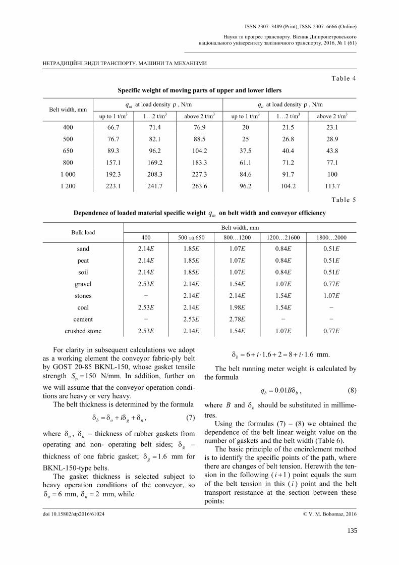
The specific weight of moving parts of upper and lower idlers is determined by formulas:
' 'ui i iq G l= ; (5)
" "li i iq G l= , (6)
where 'iG , "
iG – weight of rotating parts of upper and lower idlers respectively.
The spacing of upper and lower idlers il on the path is taken according to the table 8.3 [8]. The lower row idlers are arranged with the double
il spacing.
Using the data from tables 8.3 – 8.5 [8] and the formulas (5) – (6) we calculate the specific weight of moving parts of upper and lower idlers. The fol-lowing table shows the values of the specific weight of moving parts of upper and lower idlers depending on the belt width and load density.
Using the data in table 1 and the formula (4), we built dependence of the loaded material specific weight on the belt width and the conveyor effi-ciency. The resulted data are shown in Table 5.
Table 2
Ranges of ratio values E kβ corresponding to type of load and belt width
Ranges of ratio values E kβ , t/h, with the belt width, mm Bulk load
Specific weight of moving parts of upper and lower idlers
uiq at load density ρ , N/m liq at load density ρ , N/m Belt width, mm
up to 1 t/m3 1…2 t/m3 above 2 t/m3 up to 1 t/m3 1…2 t/m3 above 2 t/m3
400 66.7 71.4 76.9 20 21.5 23.1
500 76.7 82.1 88.5 25 26.8 28.9
650 89.3 96.2 104.2 37.5 40.4 43.8
800 157.1 169.2 183.3 61.1 71.2 77.1
1 000 192.3 208.3 227.3 84.6 91.7 100
1 200 223.1 241.7 263.6 96.2 104.2 113.7
Table 5
Dependence of loaded material specific weight mq on belt width and conveyor efficiency
Belt width, mm Bulk load
400 500 та 650 800…1200 1200…21600 1800…2000
sand 2.14E 1.85E 1.07E 0.84E 0.51E
peat 2.14E 1.85E 1.07E 0.84E 0.51E
soil 2.14E 1.85E 1.07E 0.84E 0.51E
gravel 2.53E 2.14E 1.54E 1.07E 0.77E
stones − 2.14E 2.14E 1.54E 1.07E
coal 2.53E 2.14E 1.98E 1.54E −
cement − 2.53E 2.78E − −
crushed stone 2.53E 2.14E 1.54E 1.07E 0.77E For clarity in subsequent calculations we adopt
as a working element the conveyor fabric-ply belt by GOST 20-85 BKNL-150, whose gasket tensile strength р 150S = N/mm. In addition, further on we will assume that the conveyor operation condi-tions are heavy or very heavy.
The belt thickness is determined by the formula
b o g niδ = δ + δ + δ , (7)
where oδ , nδ – thickness of rubber gaskets from operating and non- operating belt sides; gδ – thickness of one fabric gasket; 1.6gδ = mm for BKNL-150-type belts.
The gasket thickness is selected subject to heavy operation conditions of the conveyor, so
6oδ = mm, 2nδ = mm, while
6 1.6 2 8 1.6b i iδ = + ⋅ + = + ⋅ mm.
The belt running meter weight is calculated by the formula
0.01b bq B= δ , (8)
where B and bδ should be substituted in millime-tres.
Using the formulas (7) – (8) we obtained the dependence of the belt linear weight value on the number of gaskets and the belt width (Table 6).
The basic principle of the encirclement method is to identify the specific points of the path, where there are changes of belt tension. Herewith the ten-sion in the following ( 1i + ) point equals the sum of the belt tension in this ( i ) point and the belt transport resistance at the section between these points:
135
ISSN 2307–3489 (Print), ІSSN 2307–6666 (Online)
Наука та прогрес транспорту. Вісник Дніпропетровського національного університету залізничного транспорту, 2016, № 1 (61)
Belt tension at point 2 is calculated by the for-mula 2 1 12S S W= + , (10)
where 12W – belt transport resistance at the section between the points 1 and 2;
( )12 г b liW wL q q= + . (11)
where w – belt transport resistance (Table 7), which depends on the type of bearing, lubrication, sealing, dustiness of atmosphere and other condi-tions.
For further research it is assumed that 0.03w = (operation conditions are heavy, lower idlers are straight, upper idlers are grooved). Using the tables 5 and 6, we obtained the expressions for tension force values at point 2, depending on the belt width and load density (Table 8).
Belt tension at point 3 is calculated by the for-mula 3 2S k S= , (12)
where k – coefficient for increase in belt tension due to idler pulley rotating resistance (Table 9).
In the considered conveyor design the belt wrap angle of pulley is less than 90o (Fig. 1), thus
1.03k = . Table 9
Value of coefficient k
Belt wrap angle of pulley, degrees k
<90 1.03
90 1.04
180 1.05 Dependencies to determine the tension force
value at point 3 by belt width and load density are shown in Table 10.
Belt tension at point 4 is calculated by the for-mula 4 3 34S S W= + , (13)
where 34W – belt transport resistance at the section between the points 3 and 4;
( )34 34 34cos sinb liW q L w q L w= ⋅ β − β + , (14)
where w – belt transport resistance coefficient (Table 7).
If 0.03w = (operation conditions are heavy, lower idlers are straight), then the dependences for tension force values at point 4 by belt width and load density are shown in Table 11.
Belt tension at point 5 is calculated by the for-mula 5 4S k S= , (15)
where k – coefficient for increase in belt tension due to idler pulley rotating resistance (Table 9).
In the considered conveyor design the belt wrap angle of pulley is 180o (Fig. 1), therefore, we as-sume that 1.05k = .
Dependencies for tension force values at point 5 by belt width and load density are shown in Ta-ble 12.
Belt tension at point 6 is calculated by the for-mula
6 5 56S S W= + , (16)
where 56W – belt transport resistance at the section between the points 5 and 6;
( ) ( )56 56 56cos sinm b uiW q q L w q L w= + ⋅ β + β + , (17)
where w – belt transport resistance coefficient (Table 7).
If 0.03w = (operation conditions are heavy, upper idlers are grooved), then the dependences for tension force values at point 6 by belt width and load density are shown in Table 13.
Belt tension at point 7 is calculated by Euler’s formula:
7 6wS S e α= , (18)
where w – friction factor between the belt and the idler surface; α – belt wrap angle of battery of idlers, radian.
Belt wrap angle of battery of idlers:
67
1
LR
α = . (19)
Dependencies for tension force values at point 7 by belt width and load density are shown in Ta-ble 14.
+ qmL56 (0.03cosβ+sinβ)] Belt tension at point 8 is calculated by the for-
mula
8 7 78S S W= + , (20)
where 78W – belt transport resistance at the section between the points 7 and 8;
( )78 78m b uiW q q q L w= + + , (21)
where w – belt transport resistance coefficient (Table 7).
If 0.03w = (operation conditions are heavy, upper idlers are grooved), then the dependences for tension force values at point 8 by belt width and load density are shown in Table 15.
140
ISSN 2307–3489 (Print), ІSSN 2307–6666 (Online)
Наука та прогрес транспорту. Вісник Дніпропетровського національного університету залізничного транспорту, 2016, № 1 (61)
We developed parametric dependence of drive power of the belt conveyer with sloping and hori-zontal areas on type of load, design efficiency, ge-ometrical dimensions and path configuration, op-eration conditions that takes into account standard
dimensions and parameters of belts, idlers and pul-leys.
Use of the built dependences gives an opportu-nity of relatively rapid determination of approxi-mate value of the drive power for the belt convey-ers of considered design, as well as it allows qual-
143
ISSN 2307–3489 (Print), ІSSN 2307–6666 (Online)
Наука та прогрес транспорту. Вісник Дніпропетровського національного університету залізничного транспорту, 2016, № 1 (61)
ity selection of its basic elements at specific design characteristics and requirements.
The proposed dependences can be used for de-termination of general impact of the design effi-ciency and other parameters on the conveyor drive power.
Conclusions
For belt conveyors with sloping and horizontal areas we built parametric dependence of drive power on the design parameters: type of load, de-sign efficiency, geometrical dimensions and path configuration, operation conditions. Such depend-ences allow calculating the required drive power value, taking into account the type and the physical and mechanical properties of load, the lifting height value, the transport length and design effi-ciency, using only one formula, chosen depending on design characteristics.
LIST OF REFERENCE LINKS 1. Александров, М. П. Подъемно-транспортные
машины : учебник / М. П. Александров. – Мос-ква : Высш. шк., 2000. – 522 с.
2. Богомаз, В. М. Аналіз впливу проектних хара-ктеристик елеватору на параметри його приво-ду / В. М. Богомаз // Наука та прогрес транспо-рту. – 2015. – № 3 (57). – С. 162–175. doi: 10.15802/stp2015/46076.
3. Богомаз, В. М. Дослідження впливу проектної продуктивності елеватору на потужність його приводу / В. М. Богомаз, К. Ц. Главацький, О. А. Мазур // Наука та прогрес транспорту. – 2015. – № 2 (56). – С. 189–206. doi: 10.15802/stp2015/42178.
4. Зенков, Р. Л. Машины непрерывного транспор-та : учебник / Р. Л. Зенков, И. И. Ивашков, Л. Н. Колобов. – Москва : Машиностроение, 1987. – 432 с.
5. Іванченко, Ф. К. Підйомно-транспортні маши-ни : підручник / Ф. К. Іванченко. – Київ : Вища шк., 1993. – 413 с.
6. Катрюк, И. С. Машины непрерывного транс-порта. Конструкции, проектирование и экс-плуатация: учеб. пособие / И. С. Катрюк, Е. В. Мусияченко. – Красноярск : ИПЦ КГТУ, 2006. – 266 с.
7. Кузьмин, А. В. Справочник по расчетам меха-низмов подъемно-транспортных машин : учебн. пособие / А. В. Кузьмин. – Минск : Вы-шэйшая школа, 1983. – 350 с.
8. Підйомно-транспортні машини: розрахунки підіймальних і транспортувальних машин : підручник / В. С. Бондарєв, О. І. Дубинець, М. П. Колісник [та ін.]. – Київ : Вища шк., 2009. – 734 с.
9. Расчет и проектирование транспортних средств непрерывного действия : научное пособие для вузов / А. И. Барышев, В. А. Будишевский, А. А. Сулима, А. М. Ткачук. – Донецк : Норд-Пресс, 2005. – 689 с.
10. Ромакин, Н. Е. Машины непрерывного транс-порта : учебн. пособие / Н. Е. Ромакин. – Мос-ква : Академия, 2008. – 432 с.
11. Jamaludin, J. Development of a self-tuning fuzzy logic controller for intelligent control of elevator systems / J. Jamaludin, N. A. Rahim, W. P. Hew // Engineering Applications of Artificia Intelligence. – 2009. – Vol. 22. – Iss. 8. – Р. 1167–1178. doi: 10.1016/j.engappai.2009.04.006.
12. Kim, C. S. Nonlinear robust control of a hydraulic elevator: experiment-based modeling and two-stage Lyapunov redesign / C. S. Kim, K. S. Hong, M. K. Kim // Control Engineering Practice. – 2005. – Vol. 13. – Iss. 6. – P. 789–803. doi: 10.1016/j.conengprac.2004.09.003.
13. Strakosch, G. R. The Vertical Transportation Handbook / G. R. Strakosch, R. S. Caporale. – New York : John Wiley&Sons, 2010. – 610 p. doi: 10.1002/9780470949818.
В. М. БОГОМАЗ1*
1*Каф. «Військова підготовка спеціалістів Державної спеціальної служби транспорту», Дніпропетровський національний університет залізничного транспорту імені академіка В. Лазаряна, вул. Лазаряна, 2, Дніпропетровськ, Україна, 49010, тел. +38 (056) 793 19 09, ел. пошта [email protected], ORCID 0000-0001-5913-2671
ДОСЛІДЖЕННЯ ЗАЛЕЖНОСТІ ПОТУЖНОСТІ ПРИВОДУ СТРІЧКОВОГО КОНВЕЄРУ ВІД ЙОГО ПРОЕКТНИХ ПАРАМЕТРІВ
Мета. Привід є одним із основних елементів стрічкових конвеєрів. Для визначення потужності приводу необхідно провести розрахунки за стандартними методиками, які викладені в сучасній технічній літературі. Для таких розрахунків потрібно витратити достатньо багато часу. Основними проектними параметрами
144
ISSN 2307–3489 (Print), ІSSN 2307–6666 (Online)
Наука та прогрес транспорту. Вісник Дніпропетровського національного університету залізничного транспорту, 2016, № 1 (61)
стрічкового транспортера є: тип вантажу, проектна продуктивність, геометричні розміри та конфігурація траси, умови роботи. В статті необхідно побудувати параметричну залежність потужності приводу стрічко-вого конвеєру від проектних параметрів, яка враховувала б стандартні розміри і параметри стрічок, ролико-опор та барабанів. Методика. Розглядається стрічковий конвеєр із двома ділянками: похилою та горизонта-льною. Використовуючи методику тягового розрахунку способом обходу по контуру стрічкових конвеєрів, побудовано параметричні залежності сил натягу в характерних точках траси конвеєру від типу вантажу, проектної продуктивності, геометричних розмірів та конфігурації траси конвеєру, умов роботи. Результати. Для стрічкових конвеєрів розглянутого типу з врахуванням стандартних розмірів стрічки та відповідними припущеннями щодо типу роликоопор та барабанів побудовано параметричні залежності потужності приво-ду від типу вантажу, проектної продуктивності, геометричних розмірів і конфігурації траси конвеєру, умов роботи. Наукова новизна. Вперше побудована параметрична залежність потужності приводу стрічкових конвеєрів із двома ділянками (похилою та горизонтальною) від типу вантажу, проектної продуктивності, геометричних розмірів та конфігурації траси конвеєру, умов роботи. Вона враховує стандартні розміри та параметри стрічок, роликоопор і барабанів. Практична значимість. Використання побудованих залежнос-тей потужності приводу стрічкових конвеєрів із похилою та горизонтальною ділянками від проектних пара-метрів дає можливість відносно швидкого визначення приблизного значення потужності приводу на стадії проектування. Також можливим є виконання якісного підбору його основних елементів при конкретних проектних характеристиках та вимогах. Запропоновані залежності можуть бути використані для визначення загального характеру залежності потужності приводу від проектної продуктивності.
1*Каф. «Военная подготовка специалистов Государственной специальной службы транспорта», Днепропетровский национальний университет железнодорожного транспорта имени академика В. Лазаряна, ул. Лазаряна, 2, Днепропетровск, Украина, 49010, тел. +38 (056) 793 19 09, эл. почта [email protected], ORCID 0000-0001-5913-2671
ИССЛЕДОВАНИЕ ЗАВИСИМОСТИ МОЩНОСТИ ПРИВОДА ЛЕНТОЧНОГО КОНВЕЙЕРА ОТ ЕГО ПРОЕКТНЫХ ПАРАМЕТРОВ
Цель. Привод является одним из основных элементов ленточных конвейеров. Для определения мощно-сти привода необходимо провести расчеты по стандартным методикам, которые изложены в современной технической литературе. Для таких расчетов нужно потратить достаточно много времени. Основными про-ектными параметрами ленточных транспортеров являются: тип груза, проектная производительность, гео-метрические размеры и конфигурация трассы, условия работы. В статье необходимо построить параметри-ческую зависимость мощности привода ленточного конвейера от его проектных параметров, которая учиты-вала б стандартные размеры и параметры лент, роликоопор и барабанов. Методика. Рассматривается лен-точный конвейер с двумя участками: наклонным и горизонтальным. Используя методику тягового расчета способом обхода по контуру ленточных конвейеров, построены параметрические зависимости сил натяже-ния в характерных точках трассы конвейера от типа груза, проектной производительности, геометрических размеров и конфигурации трассы, условий работы. Результаты. Для ленточных конвейеров рассмотренного типа с учетом стандартных размеров ленты и соответствующими предположениями относительно типов роликоопор и барабанов построены параметрические зависимости мощности привода от типа груза, проектной производительности, геометрических размеров и конфигурации трассы, условий работы. Научная новизна. Впервые построена параметрическая зависимость мощности привода ленточных конвейеров с двумя участками (наклонной и горизонтальной) от типа груза, проектной производительности, геометрических размеров и конфигурации трассы, условий работы. Она учитывает стандартные размеры и параметры ленты, роликоопор и барабанов. Практическая значимость. Использование построенных зависимостей мощности привода ленточных конвейеров с наклонным и горизонтальным участками дает возможность относительно быстрого определения приблизительного значения мощности привода на стадии проектирования. Также возможным является выполнение качественного подбора его основных элементов при конкретных проектных характеристиках и требованиях. Предложенные зависимости могут быть использованы для определения общего характера зависимости мощности привода от проектной производительности.
REFERENCES 1. Aleksandrov M.P. Podemno-transportnyye mashiny [Lifting and transport machines]. Moscow, Vysshaya
shkola Publ., 2000. 522 p. 2. Bohomaz V.M. Analiz vplyvu proektnykh kharakterystyk elevatoru na parametry yoho pryvodu [Influence
analyses of designed characteristics of the elevator to the parameters of its drive]. Nauka ta prohres transportu – Science and Transport Progress, 2015, no. 3 (57), pp. 162-175. doi: 10.15802/stp2015/46076.
3. Bohomaz V.M., Hlavatskyi K.Ts., Mazur O.A. Doslidzhennia vplyvu proektnoi produktyvnosti elevatoru na potuzhnist yoho pryvodu [Research of influencing of project discriptions of elevator on parameters of its drive]. Nauka ta prohres transportu – Science and Transport Progress, 2015, no. 2 (56), pp. 189-206. doi: 10.15802/stp2015/42178.
4. Zenkov R.L., Ivashkov I.I., Kolobov L.N. Mashiny nepreryvnogo transporta [Machines of continuous trans-port]. Mosocw, Mashinostroeniye Publ., 1987. 432 p.
5. Ivanchenko F.K. Pidiomno-transportni mashyny [Lifting and transport machines]. Kyiv, Vyshcha shkola Publ., 1993. 413 p.
6. Katryuk I.S., Musiyachenko Ye.V. Mashiny nepreryvnogo transporta. Konstruktsii, proyektirovaniye i ek-spluatatsiya [Machines of continuous transport. Construction, design and operation]. Krasnoyarsk, IPTs KGTU Publ., 2006. 266 p.
7. Kuzmin, A.V. Spravochnik po raschetam mekhanizmov podemno-transportnykh mashin [Manual of calcula-tion mechanisms of lifting and transport machines]. Minsk, Vysheyshaya shkola Publ., 1983. 350 p.
8. Bondariev V.S., Dubynets O.I., Kolisnyk M.P. Pidiomno-transportni mashyny: rozrakhunky pidiimalnykh i transportuvalnykh mashyn [Lifting and transport machines: calculations of hoisting and conveying machines]. Kyiv, Vyshcha shkola Publ., 2009. 734 p.
9. Baryshev A. I., Budishevskiy V. A., Sulima A. A., Tkachuk A. M. Raschet i proyektirovaniye transportnykh sredstv nepreryvnogo deystviya [Calculation and design of continuous action vehicles]. Donetsk, Nord-Press Publ., 2005. 689 p.
10. Romakin N.Ye. Mashiny nepreryvnogo transporta [Machines of continuous transport]. Moscow, Akademiya Publ., 2008. 432 p.
11. Jamaludin J., Rahim N.A., Hew W.P. Development of a self-tuning fuzzy logic controller for intelligent con-trol of elevator systems. Engineering Applications of Artificial Intelligence, 2009, vol. 22, issue 8, pp. 1167-1178. doi: 10.1016/j.engappai.2009.04.006.
12. Kim C.S., Hong K.S., Kim M.K. Nonlinear robust control of a hydraulic elevator: experiment-based modeling and two-stage Lyapunov redesign. Control Engineering Practice, 2005, vol. 13, issue 6, pp. 789-803. doi: 10.1016/j.conengprac.2004.09.003.
13. Strakosch G.R., Caporale R.S. The Vertical Transportation Handbook. New York, John Wiley&Sons Publ., 2010. 610 p. doi: 10.1002/9780470949818.
Prof. S. V. Raksha, Sc. Tech. (Ukraine); Assos. Prof. S. V. Shatov, Sc. Tech. (Ukraine) recommended
this article to be published Accessed: Nov., 20. 2015 Received: Jan., 15. 2016