Power amplifier linearization technique with IQimbalance and crosstalk compensation forbroadband MIMO-OFDM transmittersFernando Gregorio1*, Juan Cousseau1, Stefan Werner2, Taneli Riihonen2 and Risto Wichman2
Abstract
The design of predistortion techniques for broadband multiple input multiple output-OFDM (MIMO-OFDM) systemsraises several implementation challenges. First, the large bandwidth of the OFDM signal requires the introductionof memory effects in the PD model. In addition, it is usual to consider an imbalanced in-phase and quadrature (IQ)modulator to translate the predistorted baseband signal to RF. Furthermore, the coupling effects, which occurwhen the MIMO paths are implemented in the same reduced size chipset, cannot be avoided in MIMOtransceivers structures. This study proposes a MIMO-PD system that linearizes the power amplifier response andcompensates nonlinear crosstalk and IQ imbalance effects for each branch of the multiantenna system. Efficientrecursive algorithms are presented to estimate the complete MIMO-PD coefficients. The algorithms avoid the highcomputational complexity in previous solutions based on least squares estimation. The performance of theproposed MIMO-PD structure is validated by simulations using a two-transmitter antenna MIMO system. Errorvector magnitude and adjacent channel power ratio are evaluated showing significant improvement comparedwith conventional MIMO-PD systems.
1. IntroductionEmerging broadband communication systems requirehigh spectral efficiency and robustness against multipathchannels. For this reason, OFDM has been adopted inthe majority of modern wireless communication stan-dards. Furthermore, multiantenna transceivers representone of the most prominent techniques to enhance systemcapacity. Mobile WiMAX, LTE, Ultra Wide Band, andWLAN (IEEE 802.11n) allow the use of MIMO-OFDM(multiple input multiple output-OFDM) in their specifi-cations. However, several factors should be considered toobtain the advantages promised by MIMO techniques.The high dynamic range of OFDM signals imposes theuse of linear amplifiers (class A and class AB). Therequirement of linear amplifiers, with a poor power duty,creates a problem accentuated by the use of multipleantennas. The high-data transmission rates, reached with
the combination of OFDM and MIMO contrast with theloss of portability of the product, because of their ele-vated power consumption. Therefore, there is a trade-offbetween the high data rate obtained by employingMIMO techniques and the high power consumption ofthe OFDM system. Furthermore, when considering low-cost components, there are also several imperfections/impairments that degrade the system performance andneed to be taken into account in the design of a compen-sation system.Despite several advantages, OFDM is sensitive to dis-
tortions introduced at the RF front-end. InexpensiveOFDM transceivers employing direct conversion archi-tectures (zero intermediate frequency) are seriouslyaffected by front-end distortions, e.g., in-phase and quad-rature (IQ) baseband imbalance and phase noise. In addi-tion, OFDM transceivers are also intrinsically sensitive topower amplifier (PA) nonlinear distortion. Nonlinear PAcreates spectral regrowth (out-of-band distortion) and in-band distortion that degrades the system’s bit error rate(BER). The trade-off between power efficiency and
* Correspondence: [email protected] of Electrical and Computer Engineering, UniversidadNacional del Sur, Av. Alem 1253, Bahía Blanca 8000, ArgentinaFull list of author information is available at the end of the article
Gregorio et al. EURASIP Journal on Advances in Signal Processing 2011, 2011:19http://asp.eurasipjournals.com/content/2011/1/19
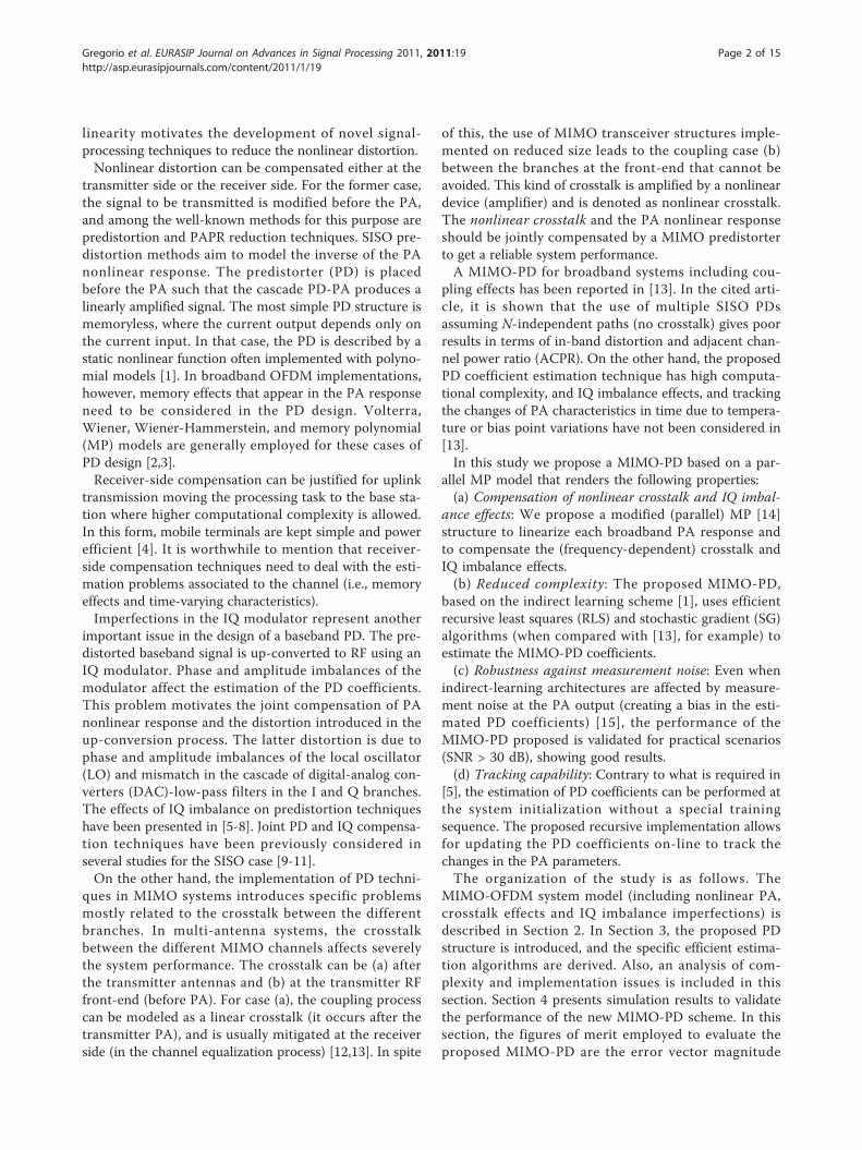
linearity motivates the development of novel signal-processing techniques to reduce the nonlinear distortion.Nonlinear distortion can be compensated either at the
transmitter side or the receiver side. For the former case,the signal to be transmitted is modified before the PA,and among the well-known methods for this purpose arepredistortion and PAPR reduction techniques. SISO pre-distortion methods aim to model the inverse of the PAnonlinear response. The predistorter (PD) is placedbefore the PA such that the cascade PD-PA produces alinearly amplified signal. The most simple PD structure ismemoryless, where the current output depends only onthe current input. In that case, the PD is described by astatic nonlinear function often implemented with polyno-mial models [1]. In broadband OFDM implementations,however, memory effects that appear in the PA responseneed to be considered in the PD design. Volterra,Wiener, Wiener-Hammerstein, and memory polynomial(MP) models are generally employed for these cases ofPD design [2,3].Receiver-side compensation can be justified for uplink
transmission moving the processing task to the base sta-tion where higher computational complexity is allowed.In this form, mobile terminals are kept simple and powerefficient [4]. It is worthwhile to mention that receiver-side compensation techniques need to deal with the esti-mation problems associated to the channel (i.e., memoryeffects and time-varying characteristics).Imperfections in the IQ modulator represent another
important issue in the design of a baseband PD. The pre-distorted baseband signal is up-converted to RF using anIQ modulator. Phase and amplitude imbalances of themodulator affect the estimation of the PD coefficients.This problem motivates the joint compensation of PAnonlinear response and the distortion introduced in theup-conversion process. The latter distortion is due tophase and amplitude imbalances of the local oscillator(LO) and mismatch in the cascade of digital-analog con-verters (DAC)-low-pass filters in the I and Q branches.The effects of IQ imbalance on predistortion techniqueshave been presented in [5-8]. Joint PD and IQ compensa-tion techniques have been previously considered inseveral studies for the SISO case [9-11].On the other hand, the implementation of PD techni-
ques in MIMO systems introduces specific problemsmostly related to the crosstalk between the differentbranches. In multi-antenna systems, the crosstalkbetween the different MIMO channels affects severelythe system performance. The crosstalk can be (a) afterthe transmitter antennas and (b) at the transmitter RFfront-end (before PA). For case (a), the coupling processcan be modeled as a linear crosstalk (it occurs after thetransmitter PA), and is usually mitigated at the receiverside (in the channel equalization process) [12,13]. In spite
of this, the use of MIMO transceiver structures imple-mented on reduced size leads to the coupling case (b)between the branches at the front-end that cannot beavoided. This kind of crosstalk is amplified by a nonlineardevice (amplifier) and is denoted as nonlinear crosstalk.The nonlinear crosstalk and the PA nonlinear responseshould be jointly compensated by a MIMO predistorterto get a reliable system performance.A MIMO-PD for broadband systems including cou-
pling effects has been reported in [13]. In the cited arti-cle, it is shown that the use of multiple SISO PDsassuming N-independent paths (no crosstalk) gives poorresults in terms of in-band distortion and adjacent chan-nel power ratio (ACPR). On the other hand, the proposedPD coefficient estimation technique has high computa-tional complexity, and IQ imbalance effects, and trackingthe changes of PA characteristics in time due to tempera-ture or bias point variations have not been considered in[13].In this study we propose a MIMO-PD based on a par-
allel MP model that renders the following properties:(a) Compensation of nonlinear crosstalk and IQ imbal-
ance effects: We propose a modified (parallel) MP [14]structure to linearize each broadband PA response andto compensate the (frequency-dependent) crosstalk andIQ imbalance effects.(b) Reduced complexity: The proposed MIMO-PD,
based on the indirect learning scheme [1], uses efficientrecursive least squares (RLS) and stochastic gradient (SG)algorithms (when compared with [13], for example) toestimate the MIMO-PD coefficients.(c) Robustness against measurement noise: Even when
indirect-learning architectures are affected by measure-ment noise at the PA output (creating a bias in the esti-mated PD coefficients) [15], the performance of theMIMO-PD proposed is validated for practical scenarios(SNR > 30 dB), showing good results.(d) Tracking capability: Contrary to what is required in
[5], the estimation of PD coefficients can be performed atthe system initialization without a special trainingsequence. The proposed recursive implementation allowsfor updating the PD coefficients on-line to track thechanges in the PA parameters.The organization of the study is as follows. The
MIMO-OFDM system model (including nonlinear PA,crosstalk effects and IQ imbalance imperfections) isdescribed in Section 2. In Section 3, the proposed PDstructure is introduced, and the specific efficient estima-tion algorithms are derived. Also, an analysis of com-plexity and implementation issues is included in thissection. Section 4 presents simulation results to validatethe performance of the new MIMO-PD scheme. In thissection, the figures of merit employed to evaluate theproposed MIMO-PD are the error vector magnitude
Gregorio et al. EURASIP Journal on Advances in Signal Processing 2011, 2011:19http://asp.eurasipjournals.com/content/2011/1/19
Page 2 of 15
(EVM) and the ACPR. Finally, Section 5 concludes thearticle.To simplify the notation, we develop the MIMO-PD
for M = 2 transmit antennas. However, the proposedtechnique is not restricted to this case and can easily begeneralized to M > 2 transmit antennas.Throughout this article, we employ the following
abbreviations. MIMO-PD denotes MIMO predistorter,and CPD represents conventional predistorter. MIMO-PD SG, MIMO-PD RLS, and MIMO-PD LS areemployed to define the MIMO predistorters coefficientsof which were obtained using stochastic gradient, recur-sive least squares, and least squares algorithms, respec-tively. The acronyms MP and MLP denote memory andmemoryless polynomials.
2. System ModelThe transmitter front-end considered uses direct-conversion architecture [16]. This architecture presentsseveral advantages when compared with the conven-tional super-heterodyne structure: small number ofparts, low-mixing product spurs, few filters, and lowcurrent consumption [17].Let {X�(k)}N−1
k=0 ∈ C be the modulated data symbolsassociated with carrier k to be transmitted by antennaℓ = 1, 2,..., M. The time-domain OFDM symbols{x�(n)}N−1
n=0 are obtained via the inverse discrete Fouriertransform:
x�(n) =1√N
N−1∑k=0
X�(k)ej2π
Nkn, n = 0, 1, . . . , N − 1. (1)
The OFDM signal xℓ(n) at the transmitter is separatedinto real and imaginary (IQ) digital baseband compo-nents, xiℓ(n) and xqℓ(n). The IQ components are filteredby the I and Q branches equivalent low-pass filters,hiℓ(n) and hqℓ(n), and converted to continuous-timebaseband signals, xi�(t) and xq�(t).The low-pass filters hiℓ(n) and hqℓ(n), which model the
cascade of DAC and the analog low-pass filters, arerepresented as FIR filters of lengths Li and Lq, respec-tively [18]. Generically, the impulse responses hiℓ(n) andhqℓ(n) are different, creating an IQ frequency-dependentmismatch.The IQ components at the low-pass filters output
(continuous-time baseband signals) are directly modu-lated to RF, xrfℓ(t), using two LO signals ideally in quad-rature. However, in “real-life” implementations, LOsignals present phase and amplitude imbalances in the Iand Q branches. Amplitude- and phase imbalance para-meters of the IQ-modulator associated to the branch ℓ
are denoted as bℓ and ϑℓ, respectively [19]. Finally, theRF signal xrfℓ(t) is amplified and transmitted through the
channel, yℓ(t). A block diagram of the transmitter front-end of the ℓ branch is illustrated in Figure 1.Following the model described in [18], the equivalent
discrete-time baseband signal after IQ modulator foreach branch of the MIMO transmitter can be repre-sented by
s�(n) = g1�(n) ⊗ x�(n) + g2�(n) ⊗ x∗�(n) (2)
where ⊗ denotes convolution, g1ℓ(n) and g2ℓ(n) areequivalent filters with impulse response given by
g1�(n) = hi�(n) + β�hq�(n)ejϑ�
g2�(n) = hi�(n) − β�hq�(n)ejϑ� .(3)
Besides IQ imbalance, direct conversion transceiverssuffer from DC offset because of LO leakage [20], themixing of the LO signal with itself and noise from themixers, filters, and DAC converters. The output of theIQ modulator including the DC offset term can be writ-ten as
u�(n) = g1�(n) ⊗ x�(n) + g2�(n) ⊗ x∗�(n) + ε� (4)
where εℓ is the DC offset term due to imperfections atthe up-converter. A block diagram of the described two-antenna MIMO-OFDM transmitter front-end (equiva-lent baseband model) is illustrated in Figure 2.The IQ imbalance model given by (2) is composed by
two branches and motivates the parallel structure of ourMIMO-PD as presented in the next section.MIMO transceiver RF front-end requires a careful
design to isolate the different branches. Nevertheless,when considering reduced-size implementation (chip-set), the coupling between the MIMO branches cannotbe fully eliminated. To model this kind of crosstalkwhich is assumed frequency dependent, we consider theoutput of the PAs, written as
y�(n) = p�
⎡⎣u�(n) +
M∑m=1,m�=�
cm�(n) ⊗ um(n)
⎤⎦ + v�(n) (5)
where pℓ[·] is the PA response of each branch, um(n)is the output of the IQ modulator of the m pathof the transceiver, and cmℓ(n) is the filter representingthe crosstalk with impulse response,cm� = [cm�(n), cm�(n − 1), . . . cm�(n − Lcm + 1)]T andmodeling the coupling between path m to path ℓ. Themeasurement noise at the output of each PA is denotedby vℓ(n). Equation 5 allows inferring that to obtain a dis-tortion-free signal xℓ(n), the PD should be able to invertthe PA response pℓ[·], remove the undesired coupledsignal, and mitigate the effects of the IQ imbalance.
Gregorio et al. EURASIP Journal on Advances in Signal Processing 2011, 2011:19http://asp.eurasipjournals.com/content/2011/1/19
Gregorio et al. EURASIP Journal on Advances in Signal Processing 2011, 2011:19http://asp.eurasipjournals.com/content/2011/1/19
Page 4 of 15
3. MIMO PredistorterOwing to the effects of crosstalk and IQ imbalance, theMIMO transmitter to be linearized follows a character-istic that can be described by a parallel nonlinear model.We consider, for the derivation, the linearization of oneMIMO path. The PD coefficients are estimated using anindirect learning structure [1]. In this methodology, theMIMO-PD parameters are estimated and copied to thepredistorter avoiding the inverse model estimationrequired by direct learning techniques. However, despiteseveral advantages, the indirect learning structure isaffected by measurement noise at the PA output [9,15].Measurement noise creates a bias in the estimatedmodel, which increases with the model order. Theeffects of the measurement noise on the proposed tech-nique are discussed and evaluated following a specificapplication in Section 4.The proposed identification structure requires a feed-
back path where the RF signal at the output of the PAis down-converted and translated to baseband. Thecomponents of the down-converter, filters, DAC, andmixer need to be carefully designed in order to mini-mize its harmful effects over the performance of theidentification technique. In this approach of this study,an ideal feedback path is considered. It is assumed thatthe demodulation is implemented digitally minimizingthe demodulation errors. A feedback path without IQdemodulator imbalance and nonlinear effects was alsoconsidered in previous publications [8-10]. In [5,11],errors in the feedback loop and techniques to removeits harmful effects are addressed. However, only fre-quency-independent imbalances are considered.
A. MIMO predistorter structureEven when other alternatives are possible, the proposedMIMO predistorter is based on the MP model [14].That model has been employed in predistortion techni-ques showing a very good performance [2]. The maincharacteristics of the MP model, which we exploitregarding real-time applications are its modularity andsimplicity.Furthermore, alternative modeling of the static part of
the MP can also be considered. Orthogonal polynomialsalleviate the ill-conditioned problems associated withthe conventional polynomial models [21]. GeneralizedMP proposed by Morgan [14] should also be an inter-esting option with improved stability at a reasonableincrease of the implementation complexity, but its use isnot discussed here.To include all the impairments, i.e., the nonlinear dis-
tortion and memory effects due to the PA, crosstalkcoupling due to the MIMO structure, and the IQ imbal-ance distortion, we propose for each PA (of the M-
antenna MIMO system) a (2 + 2(M - 1)) × 1 MISO PD.Each branch of the MISO PD is formed by a MP [14].There are two branches to model the own PA nonlineardistortion (associated to the IQ components of the IQimbalance characterization) and 2(M - 1) to model thecrosstalk associated to the other PAs.The proposed MISO PD structure, for the case M = 2,
is depicted in Figure 3. Each block P�,i denotes the MPassociated to the branch i of antenna ℓ. Based on theM = 2 case, the (4 × 1) PD output associated to antennaℓ can be written as
d�(n) =P�1−1∑p=0
M�1∑k=0
θ(�,1)pk (n)ψ∗
1p(n − k) +P�2−1∑p=0
M�2∑k=0
θ(�,2)pk (n)ψ1p(n − k)
+P�3−1∑p=0
M�3∑k=0
θ(�,3)pk (n)ψ∗
2p(n − k) +P�4−1∑p=0
M�4∑k=0
θ(�,4)pk (n)ψ2p(n − k) + ε′
�
=4∑i=1
d�,i(n) + ε′�
(6)
where θ(�,1)pk and θ
(�,2)pk denote the MP coefficients asso-
ciated to the input signal and its conjugate, respectively;
θ(�,3)pk and θ
(�,4)pk are the coefficients associated to the
crosstalk signal and its conjugate. The basis function ofthe corresponding MPs are defined byψ1p(n) = y1(n)|y1(n)|2p and ψ2p(n) = y2(n)|y2(n)|2p. Pℓi
and Mℓi are the polynomial order and memory depth ofthe branch i, respectively. The coefficient ε′
� representsthe DC offsets that arise from the IQ modulators asso-ciated to the branches 1 and 2 of the transceiver.It is straightforward to extend (6) to the more general
case of M-antennas MIMO-PD by including, instead ofthe terms d�,3(n) and d�,4(n), the corresponding 2(M -1) terms characterizing the nonlinear crosstalk from theother branches.According to the two-antenna PD to simplify the
Gregorio et al. EURASIP Journal on Advances in Signal Processing 2011, 2011:19http://asp.eurasipjournals.com/content/2011/1/19
Page 5 of 15
The PD output of the branch ℓ can be written as
d�(n) = φH� (n)θ �(n) + ε′
�. (10)
To account for the DC offset from the LO an extracoefficient, ε′
�, is added to the coefficient vector. Usingan augmented coefficient vector, the PD output signalcan be expressed as
d�(n) = φH� (n)θ �(n) (11)
where
φ�(n) = [1,φ�]T
θ�(n) = [ε, θ �]T(12)
where the augmented coefficient vector has dimen-sions 1 × (Pℓ1Mℓ1 + Pℓ2Mℓ2 + Pℓ3Mℓ3 + Pℓ4Mℓ4 + 1).
B. MIMO predistorter identification schemesTo estimate the MP coefficients, θℓ(n) and to track thetime-varying characteristics of the PA, adaptive estima-tion algorithms are considered. We propose two differ-ent algorithms: RLS and stochastic gradient algorithms.At the initialization, the PD is bypassed, and the PDcoefficients are obtained by minimizing the error signalgiven by
Figure 3 Indirect learning structure for identifying the MIMO-PD coefficients. Blocks P1,1 to P1,4 represent the memory polynomialsassociated to branch 1, and P2,1 to P2,4 represent the memory polynomials associated to branch 2.
Gregorio et al. EURASIP Journal on Advances in Signal Processing 2011, 2011:19http://asp.eurasipjournals.com/content/2011/1/19
Page 6 of 15
Using the instantaneous squared error |eℓ(n)|2 as an
objective function, a stochastic gradient algorithm thatupdates θ �(n) is given by
trolling the convergence speed and algorithm stability.In the case of the recursive least squares algorithm,
the deterministic objective function to be minimized isgiven by
��(n) =n∑i=0
λn−i|e�(i)|2 =n∑i=0
λn−i|x�(i) − φH� (i)θ�(n)|2 (15)
where l is the forgetting factor. The update processfor the PD coefficients at each time instant n can besummarized as follows:
d�(n) = φH� (n)θ �(n − 1)
e�(n) = x�(n) − d�(n)
k(n) =λ−1P(n − 1)φ�(n)
1 + λ−1φH� (n)P(n − 1)φ�(n)
θ�(n) = θ �(n − 1) + k(n)e∗�(n)
P(n) = λ−1 (P(n − 1) − k(n)φH
� (n)P(n − 1))
(16)
where k(n) is the gain vector, and P(n) is the inversecorrelation matrix.In the RLS algorithm, the coefficient vector θℓ is initi-
alized by θℓ (0) = [0, 1,... 0], and the inverse correlationmatrix is initialized to P(0) = aI where I is a (Pℓ1Mℓ1 +Pℓ2Mℓ2 + Pℓ3Mℓ3 + Pℓ4Mℓ4 + 1) × (Pℓ1Mℓ1 + Pℓ2Mℓ2 +Pℓ3Mℓ3 + Pℓ4Mℓ4 + 1) identity matrix, and a is a largeconstant.For comparison, we discuss an extension of the least
squares (LS) algorithm of [13] that also includes IQimbalance distortion at each MIMO-PD branch, in addi-tion to nonlinear crosstalk. Also to maintain simplenotation, we discuss the two-antenna predistorter. Theestimated input signal for this case can be expressed as
x = �Hθ (17)
where
x1 =[x1(0) x1(1) · · · x1(N − 1)
]Tx2 =
[x2(0) x2(1) · · · x2(N − 1)
]T�1 =
[φ1(0) φ1(1) · · · φ1(N − 1)
]�2 =
[φ2(0) φ2(1) · · · φ2(N − 1)
] (18)
Then x = [xT1xT2]
T is a (2N × 1) vector representing theN samples of the desired PD output of each branch, Ψ =[Ψ1 Ψ2] is an (L1 + L2 + 1) × 2N matrix formed by thebasis function defined by (9) and (12) (augmented basis
function that includes an unitary term), and θ = [θT1 θ
T2]
T
is an (L1 + L2 + 1) × 1 vector formed by the MIMO-PD
coefficients (including DC compensation coefficient).The coefficients vector size is defined as
L� =∑4
i=1M�,iP�,i + 1with ℓ = 1,2. The LS solution for
(17) is given by [22]
θ =(��H)−1
�x (19)
In this estimator, the measurement noise affects thedata matrix, Ψ while in the ordinary LS solution, themeasurement noise lies in the observation vector, x. Inthis case, the estimator defined by Equation (19) iscalled Data Least Squares [23].The performance and characteristics of this extension
of the MIMO-PD of [13] are studied and comparedwith our proposal in Section 4.
4. Implementation Aspects of the MIMOPredistorterThe implementation of predistortion techniques involvestwo steps: PD coefficient estimation and predistortionusing the estimated coefficients.
A. Predistorter coefficients estimationThe dimensions of MP models, i.e., memory depth andpolynomial order, need to be carefully chosen. Using alarge polynomial order allows for coping with strongnonlinear responses which leads an improvement in thelinearization capabilities of the MIMO-PD. On the otherhand, overmodeling could deteriorate the numerical sta-bility of the PD identification algorithms [15] and couldmake the estimation algorithms more sensitive to themeasurement noise [24]. Large polynomial order alsodecreases the interval of successful compensation (thatreduces the PA dynamic range) [25]. We study thetrade-off between implementation complexity, lineariza-tion capabilities, robustness against noise, and algorithmstability by simulations in this section.1) Estimation algorithms: The complexity of the estima-
tion technique is directly related to the size of the coeffi-cient vector. For example, the two-antenna PD proposedis formed by two independent PD blocks composed offour branches, each formed by a MP. The length of thecoefficient vector of each block is given by the sum of the
coefficients length of each branch: L� =(∑4
i=1 P�iM�i
)+ 1.
In case of LS implementation, its complexity is propor-tional to L3� , O[L3� ]. For the RLS algorithm, the complexityis reduced to L2� , O[L2� ]. On the other hand, the complex-ity of stochastic gradient algorithms is proportional toL�, O[L�]. However, if the PA characteristic is highly non-linear, it results in a poorly conditioned covariance matrix.This ill-conditioned covariance is reflected in slow conver-gence, when this kind of stochastic gradient algorithms isemployed.
Gregorio et al. EURASIP Journal on Advances in Signal Processing 2011, 2011:19http://asp.eurasipjournals.com/content/2011/1/19
Page 7 of 15
In order to reduce the implementation complexity ofthe RLS algorithm, the widely linear-RLS (WL-RLS) [26]algorithm can be evaluated in a future research. It is aninteresting approach to reduce the implementation com-plexity of the RLS version of the MIMO-PD, obtainingsimilar convergence speed and robustness. This algo-rithm has an implementation complexity proportional toO[2(L�/2)2], which is computationally more economicalthan the conventional RLS.Note that the identification algorithms are not exe-
cuted for every sample. It is done periodically dependingon the variation of the PA parameters due to thermaleffects (which usually vary slowly with the time). ThePD parameter identification step is not a big consumerof computational resources because it is carried out onlyperiodically. However, it should be kept in mind thatwhen using LS algorithm, a large portion of memory isrequired to store the block of samples. In addition tothe large complexity associated to the inversion of ahuge matrix, as required by the LS implementation,memory requirements are another point that motivatesthe use of an RLS algorithm.
B. MIMO-PD implementationA MP with order Pℓi and memory depth Mℓi can beexpressed as a parallel of Mℓi MLPs of order Pℓi.Our implementation employs the input signal and its
conjugate. Moreover, the branches associated to the sig-nal and its conjugate share the same basis function, i.e.,ψ∗
�p(n) = x∗
�(n)|x�(n)|2p. For this reason, its implementa-
tion does not require extra multiplications (only a con-jugation operation).The implementation of each MLP (considering the
input signal xℓ(n) and its conjugate) requires max{Pℓi}complex-valued products to implement the basis func-tion, Pℓi + Pℓi+1 complex-valued products to weight thebasis function with the polynomial coefficients, Pℓi+1
conjugations, and Pℓi + Pℓi+1 additions. An extra addi-tion is required to compensate the DC offset.All PD block of the structure proposed (ℓ = 1,..., M)
employs the same basis functions, and so the completePD requires the implementation of only one basis func-tion (the one which have the largest polynomial order).Each branch i of the path ℓ composes the MIMO-PD, isformed by a MP implemented with Mℓi MLPs. For thisreason, to build a MP branch, the operations requiredto implement a MLP needs to be executed Mℓi timeswith i = 1,..., 2 + 2(M - 1) and ℓ = 1,..., M. The blockdiagram of a 2 × 2 MIMO-PD is depicted in Figure 4a.The structure of one branch of the MIMO-PD is illu-strated in Figure 4b. In Figure 4c, the implementation ofa MLP is detailed.
Table 1 summarizes the operations required to imple-ment the proposed MIMO-PD. For comparison, we alsoinclude the required operations to implement a conven-tional PD, CPD-1 assuming no coupling and an ideal IQmodulator, and a conventional PD, CPD-2 assumingnonlinear crosstalk compensation but not IQ imbalancereduction [13].
5. Performance EvaluationIn this section, we evaluate the performance of the pro-posed linearization techniques. First, we discuss the fig-ures of merit evaluated and then the completesimulation setup is described and discussed.
A. Figures of meritThe nonlinear effects introduced by the distortions con-sidered (the nonlinear PA, IQ imbalances, and cross-talk), create in-band and out-of-band distortions. Twofigures of merit are considered to evaluate the perfor-mance of the proposed linearization technique: theEVM (which quantifies the in-band distortion and isdirectly related to the BER), and the ACPR (which is ameasure of the effects of the out-of-band distortion onadjacent channels).EVMIn most of the standards, EVM is adopted to quantifythe amount of in-band distortion that occurs at thetransmitter side. EVM is expressed as the difference,eℓ(k), between the original constellation points, Xℓ(k),and the recovered signal affected by system imperfec-tions at the kth subcarrier of the ℓth PA. The EVM foran OFDM system formed by N subcarriers is given bythe average of EVM over active subcarriers:
ρ� =1N
N−1∑k=0
ρ�(k) =1N
N−1∑k=0
√E[|e�(k)|2]E[|X�(k)|2]
(20)
where E[·]denotes the expectation operator, E[|Xℓ(k)|2]
is the desired signal energy per symbol, rℓ(k) is theEVM at subcarrier k, and eℓ(k) is the error signal definedas eℓ(k) = Xℓ(k) - Yℓ(k), where Yℓ(k) is the received fre-quency-domain signal after down-conversion.In order to get the constellation after the PA and eval-
uate the degradation in terms of the EVM, the outputsignal is down-converted and demodulated via FFT.Since we are interested in the degradation of the trans-mitted signal, we assume that down-conversion and FFTdemodulation processes, performed to demodulate thetransmitted baseband signal, are carried by employingan ideal receiver.ACPRThe out-of-band distortion is directly related to the PAoperation point. The out-of-band emission increases
Gregorio et al. EURASIP Journal on Advances in Signal Processing 2011, 2011:19http://asp.eurasipjournals.com/content/2011/1/19
Page 8 of 15
when the PA is driven into its nonlinear operationregion. This is also the region that allows high powerefficiency. The ACPR is employed to characterize thespectral regrowth and is defined as
ACPR = 10 log10
( ∫f Y(f )df∫
fmain Y(f )df
)(21)
where Y(f ) is the power spectral distribution at theoutput of the linearized PA. fad and fmain define the fre-quency bands of the adjacent and the main channels,respectively.
For example, mobile WiMAX standard defines anspectral mask that should be fulfilled. The PA requiresto be operated as close as possible to the maximum effi-ciency point that met the ACPR and spectrum maskrequirements. If these requirements cannot be met, thenthe PA operation point must be moved, where the maskand the ACPR are fulfilled reducing the PA efficiency.The adjacent channel frequency varies with the systemapplication. In this study the ACPR is evaluated in anadjacent band (frequency offset) shifted 7 MHz from themain band.
Table 1 PD implementation complexity for the proposed MIMO-PD and conventional PDs, CPD-1 and CPD-2
Operations Proposed MIMO-PD CPD-1 CPD-2
Products
∑2M
k = 1odd
(max{M�j})(max{P�j})|j=k:k+1�=1,M +
∑M
�=1
∑2+2(M−1)
i=1M
�iP�io (240)
2∑M
�=1 M�1P�1 (96)∑M
�=1 M�1P�1 +∑M
�=1∑1+(M−1)
i=1 M�iP�i (144)
Additions∑M
�=1∑2+2(M−1)
i=1 M�iP�i + 1 (193)
∑M�=1 M�1P�1 (48)
∑M
�=1
∑1+(M−1)
i=1M�iP�i (96)
Conjugations∑2M
k = 1odd
(max{M�j})(max{P�j})|j=k:k+1�=1,M (48) - -
The numbers in brackets are calculated for a 2 × 2 MIMO-PD implemented using identical memory depth and polynomial order, Mℓ, i = 6 and Pℓ, i = P = 4 with i= 1,..., 4 and ℓ = 1, 2.
1
+
+
+ +
+
+
PD-1
PD-2
PD-12x2 MIMO-PD
X2(n1M)
1
E’�
x1(n) x2(n)
x2(n)
MLP (1, 0)
MLP (1, 1)
MLP (1, 0)
MLP (1, M11)
MLP (2, 0)
MLP (2, 1)
MLP (2, M12)
θ(1,2)10 θ
(1,2)20 θ
(1,2)P�10
θ(1,1)10 θ
(1,1)20 θ
(1,1)P�10
Z−1
Z−1 Z−1
Z−1
x
xx∗ xx∗
x|x|2 x|x|P�1
x1(n − M1,1) x2(n − M2,1)
x1(n − 1)
a)b)
c)
x1(n)
x2(n)
x1(n)
to IQ mod. input 1
to IQ mod. input 1
to IQ mod. input 2
Figure 4 The proposed MIMO-PD structure. (a) 2×2 MIMO-PD implementation, (b) one branch of the MIMO-PD composed by 2(M1,1 + M1,2)memoryless polynomials, and (c) memoryless polynomial implementation of two branches (conjugate and non-conjugate).
Gregorio et al. EURASIP Journal on Advances in Signal Processing 2011, 2011:19http://asp.eurasipjournals.com/content/2011/1/19
Page 9 of 15
B. SimulationsThe performance is validated with a two-antennaMIMO-OFDM transmitter, 16-QAM modulation onN = 1,024 subcarriers, and a bandwidth of 20 MHz. Anoversampling factor of R = 8 with an interpolation filterbased on root-raised cosine pulse shape with a roll-offfactor of 20% has been employed. The coupling betweenthe twobranch transmitter (after PA) is assumed to befrequency dependent and modeled by a FIR filter withimpulse response c21 = r2[1, 0.2] (coupling from branch2 to branch 1) and c12 = r1[1, 0.15] (coupling frombranch 1 to branch 2) where r is a coupling factoremployed to define the crosstalk level.The amplitude and phase imbalance are b1 = 5% and
ϑ1 = 5°; and b2 = 3% and ϑ1 = 3°, respectively. The fre-quency-dependent imbalance are modeled by FIR filterswith the following impulse response: hi1 = [1, 0.15] andhq1 = [1, 0.12] for the branch 1, and hi2 = [1, 0.1] andhq2 = [1, 0.12]. The DC offset are |ε1| = 0.1 and |ε2| =0.07 with signal power normalized to 1.The proposed MIMO-PD is evaluated for two differ-
ent PA models:• Power amplifier 1 (PA-1): Class A amplifier. The PA
is modeled by a Wiener model where static nonlinearitycorresponds to a solid-state power amplifier (SSPA)which is modeled by the Saleh model [27], i.e.,
g[x(n)] =|x(n)|[
1 +( |x(n)|
As
)2p]1/p
exp(j � x(n))(22)
where the parameter p = 1.2 adjusts the smoothnessof the transition from the linear region to the saturationregion, and As is the amplifier input saturation. The PAoperation point is set 2 dB from the 1-dB compressionpoint. PA memory effects are modeled with a FIR filterwith coefficients hp = [1, 0.25, 0.1].• Power amplifier 2 (PA-2): Class AB amplifier. The
PA is modeled by a Wiener model taken from [28]. Thestatic nonlinearity is modeled with a polynomial andcan be expressed as
y(n) =∑p=02
b2p+1x(n)|x(n)|2p (23)
where the complex-valued coefficients are b1 = 14.97+0.0519j, b3 = - 23.0954+4.968j, and b5 = 21.3936 +0.4305j. The linear filter is given by
A(z) =1 + 0.3z−2
1 − 0.2z−1(24)
We assume identical polynomial order and memorydepth for each PD branch, i.e., Mℓ, i = 6 and Pℓ, i = P =4 for i = 1,..., 4 and ℓ = 1, 2. However, owing to the
difference between the power of the useful signal andthe power of the conjugate component, different polyno-mial order and memory depth can be considered in eachbranch to optimize the implementation complexity [9].For PD coefficient estimation, we evaluate the RLS,
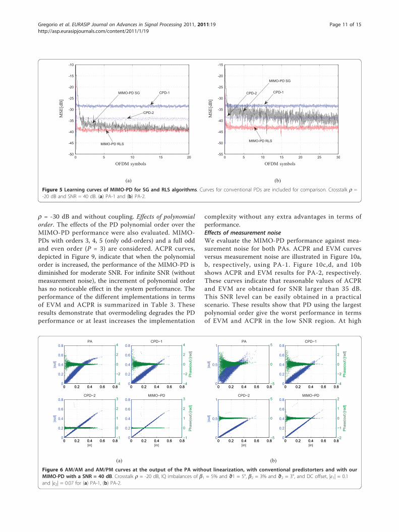
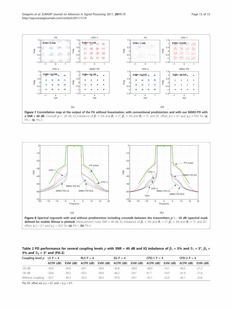
the stochastic gradient, and the LS algorithms. For com-parison, we also evaluate the performance of a conven-tional PD (CPD-1) that compensates PA memory effectsbut neglects IQ imbalance and crosstalk, i.e., it isassumed that each branch of the MIMO transceiver isdecoupled. We also implemented a conventional predis-torter, denoted CPD-2, that compensates PA effects andcrosstalk effects neglecting IQ imbalances [13].Learning curvesFigure 5a, b shows the learning curves of the MIMO-PDfor the stochastic gradient and RLS algorithms using theSSPA and class AB models, respectively. We see that forthe PA-1, the RLS algorithm only requires five OFDMsymbols to reach the MSE steady state. The stochasticgradient algorithm, which has a reduced implementationcomplexity, requires ten OFDM symbols to reach theconvergence. When conventional PDs (CPD-1, CPD-2)are used, the MSE floor is increased, reflecting this per-formance in EVM and ACPR. For the class AB PA,which presents a moderate nonlinearity at low and highamplitudes, the stochastic gradient algorithm is seriouslyaffected by a poorly conditioned covariance matrix andcannot reach the convergence even for a large trainingsequence (30 OFDM symbols). These results lead us toconclude that the RLS algorithm is the best option tothe estimation of PD coefficients.Linearization capabilitiesFigure 6 shows the AM-AM and AM-PM curves beforeand after linearization for PA-1. Identical results areobserved for our MIMO-PD estimated using stochasticgradient, RLS and LS algorithms. These curves alsoshow that conventional PDs are unable to linearize theMIMO transmitter. Residual memory effects areobserved in AM-AM and AM-PM figures. These resultscan also be observed in the constellation map at the lin-earized PA output depicted in Figure 7, where theimpact of the crosstalk and IQ imbalance can beobserved. Figures 6 and 7 had been obtained including aDC offset, |ε1| = |ε2| = 0.1.Spectral regrowth curves are shown in Figure 8 for a
measurement noise of 40 dB and crosstalk coupling r =-20 dB, using a class A PA (PA-1). In an identical sce-nario, the in-band distortion was evaluated showingEVM values around -30 dB, when using LS, RLS, andSG identification algorithms, and for a practical SNR =40 dB. Conventional PDs present a poor performancewhen the in-band distortion is evaluated, giving unsuita-ble levels of EVM. ACPR and EVM results are summar-ized in Table 2 with crosstalk coupling of r = -20 dB,
Gregorio et al. EURASIP Journal on Advances in Signal Processing 2011, 2011:19http://asp.eurasipjournals.com/content/2011/1/19
Page 10 of 15
r = -30 dB and without coupling. Effects of polynomialorder. The effects of the PD polynomial order over theMIMO-PD performance were also evaluated. MIMO-PDs with orders 3, 4, 5 (only odd-orders) and a full oddand even order (P = 3) are considered. ACPR curves,depicted in Figure 9, indicate that when the polynomialorder is increased, the performance of the MIMO-PD isdiminished for moderate SNR. For infinite SNR (withoutmeasurement noise), the increment of polynomial orderhas no noticeable effect in the system performance. Theperformance of the different implementations in termsof EVM and ACPR is summarized in Table 3. Theseresults demonstrate that overmodeling degrades the PDperformance or at least increases the implementation
complexity without any extra advantages in terms ofperformance.Effects of measurement noiseWe evaluate the MIMO-PD performance against mea-surement noise for both PAs. ACPR and EVM curvesversus measurement noise are illustrated in Figure 10a,b, respectively, using PA-1. Figure 10c,d, and 10bshows ACPR and EVM results for PA-2, respectively.These curves indicate that reasonable values of ACPRand EVM are obtained for SNR larger than 35 dB.This SNR level can be easily obtained in a practicalscenario. These results show that PD using the largestpolynomial order give the worst performance in termsof EVM and ACPR in the low SNR region. At high
0 0.2 0.4 0.6 0.80
0.2
0.4
0.6
0.8
|out
|
PA
0 0.2 0.4 0.6 0.8−4
−2
0
2
4
0 0.2 0.4 0.6 0.80
0.2
0.4
0.6
0.8CPD−1
0 0.2 0.4 0.6 0.8−4
−2
0
2
4
Pha
se(o
ut) [
rad]
0 0.2 0.4 0.6 0.80
0.2
0.4
0.6
0.8
|out
|
CPD−2
|in|0 0.2 0.4 0.6 0.8
−1
0
1
2
3
0 0.2 0.4 0.6 0.80
0.2
0.4
0.6
0.8MIMO−PD
|in|0 0.2 0.4 0.6 0.8
−1
0
1
2
3
Pha
se(o
ut) [
rad]
(a)
0 0.2 0.4 0.6 0.80
0.5
1
|out
|
PA
0 0.2 0.4 0.6 0.8−5
0
5
0 0.2 0.4 0.6 0.80
0.2
0.4
0.6
0.8CPD−1
0 0.2 0.4 0.6 0.8−4
−2
0
2
4P
hase
(out
) [ra
d]
0 0.2 0.4 0.6 0.80
0.5
1
|out
|
CPD−2
|in|0 0.2 0.4 0.6 0.8
−5
0
5
0 0.2 0.4 0.6 0.80
0.2
0.4
0.6
0.8MIMO−PD
|in|0 0.2 0.4 0.6 0.8
−2
−1
0
1
2
Pha
se(o
ut) [
rad]
(b)
Figure 6 AM/AM and AM/PM curves at the output of the PA without linearization, with conventional predistorters and with ourMIMO-PD with a SNR = 40 dB. Crosstalk r = -20 dB, IQ imbalances of b1 = 5% and ϑ1 = 5°, b2 = 3% and ϑ2 = 3°, and DC offset, |ε1| = 0.1and |ε2| = 0.07 for (a) PA-1, (b) PA-2.
0 5 10 15 20-50
-45
-40
-35
-30
-25
-20
-15
-10
MIMO-PD RLS
MIMO-PD SG
CPD-2
CPD-1
MSE
[dB]
OFDM symbols
(a)
0 5 10 15 20 25 30-55
-50
-45
-40
-35
-30
-25
-20
-15
MIMO-PD RLS
MIMO-PD SG
CPD-2 CPD-1
MSE
[dB]
OFDM symbols
(b)
Figure 5 Learning curves of MIMO-PD for SG and RLS algorithms. Curves for conventional PDs are included for comparison. Crosstalk r =-20 dB and SNR = 40 dB. (a) PA-1 and (b) PA-2.
Gregorio et al. EURASIP Journal on Advances in Signal Processing 2011, 2011:19http://asp.eurasipjournals.com/content/2011/1/19
Page 11 of 15
−20 −15 −10 −5 0 5 10 15 20−70
−60
−50
−40
−30
−20
−10
0
Frequency
PS
D
PA output
CPD−1
CPD−2
MIMO−PD SG
MIMO−PD LS MIMO−PD RLS
(a)
−20 −15 −10 −5 0 5 10 15 20−70
−60
−50
−40
−30
−20
−10
0
Frequency
PS
D
MIMO−PD SGCPD−1
CPD−2MIMO−PD LS
MIMO−PD RLSinput
PA output
(b)
Figure 8 Spectral regrowth with and without predistortion including crosstalk between the transmitters r = - 20 dB (spectral maskdefined for mobile Wimax is plotted). Measurement noise SNR = 40 dB, IQ imbalance of b1 = 5% and ϑ1 = 5°, b2 = 3% and ϑ2 = 3°, and DCoffset, |ε1| = 0.1 and |ε2| = 0.07 for (a) PA-1, (b) PA-2.
−1 0 1−1.5
−1
−0.5
0
0.5
1
1.5
imag
PA
−1 0 1−1.5
−1
−0.5
0
0.5
1
1.5
imag
CPD−1
−1 0 1−1.5
−1
−0.5
0
0.5
1
1.5
real
imag
CPD−2
−1 0 1−1.5
−1
−0.5
0
0.5
1
1.5
real
imag
MIMO−PD
EVM=−5.2dB EVM=−14.1dB
EVM=−23.5dB EVM=−30.3dB
(a)
−1 0 1−1.5
−1
−0.5
0
0.5
1
1.5
imag
PA
−1 0 1−1.5
−1
−0.5
0
0.5
1
1.5
imag
CPD−1
−1 0 1−1.5
−1
−0.5
0
0.5
1
1.5
real
imag
CPD−2
−1 0 1−1.5
−1
−0.5
0
0.5
1
1.5
real
imag
MIMO−PD
EVM=−1.5dB EVM=−14.6dB
EVM=−22.5dB EVM=−29.9dB
(b)
Figure 7 Constellation map at the output of the PA without linearization, with conventional predistorters and with our MIMO-PD witha SNR = 40 dB. Crosstalk r = -20 dB, IQ imbalance of b1 = 5% and ϑ1 = 5°, b2 = 3% and ϑ2 = 3°, and DC offset, |ε1| = 0.1 and |ε2| = 0.07 for (a)PA-1, (b) PA-2.
Table 2 PD performance for several coupling levels r with SNR = 40 dB and IQ imbalance of b1 = 5% and ϑ1 = 5°, b2 =3% and ϑ2 = 3° and (PA-2)
Coupling level r LS P = 4 RLS P = 4 SG P = 4 CPD-1 P = 4 CPD-2 P = 4
Gregorio et al. EURASIP Journal on Advances in Signal Processing 2011, 2011:19http://asp.eurasipjournals.com/content/2011/1/19
Page 12 of 15
SNR, MIMO-PDs using different polynomial ordersreach similar results.
6. Conclusions and Future WorkWe have presented a MIMO-PD that combines PAresponse linearization, IQ imbalance, and crosstalk com-pensation. Our PD shows an improved performancecompared with conventional isolated PD structures.EVM values around -30 dB, and ACPR nearer to 50 dB
are obtained with the proposed MIMO-PD in a scenariothat includes impairments at the upconversion blockmodulator and crosstalk between the different branches.Conventional PDs are unable to operate in this scenario,giving EVM and ACPR values that fail to comply withthe specifications of the majority of the wireless stan-dards. The proposed technique shows a moderate imple-mentation complexity and also includes trackingcapabilities to follow PA parameter variations. Simulation
−20 −15 −10 −5 0 5 10 15 20−70
−60
−50
−40
−30
−20
−10
0
Frequency
PS
D
input
RLS P=4 LS P=4
RLS P=5
RLS P=3 (odd terms), odd and even terms
PA output
(a)
−20 −15 −10 −5 0 5 10 15 20−70
−60
−50
−40
−30
−20
−10
0
Frequency
PS
D
RLS P=5
RLS P=4
input
PA output
(b)
-20 -15 -10 -5 0 5 10 15 20-70
-60
-50
-40
-30
-20
-10
0
Frequency
PS
D
input
RLS P=4
LS P=4RLS P=5
RLS P=3 (odd terms), odd and even terms
PA output
(c)
-20 -15 -10 -5 0 5 10 15 20-70
-60
-50
-40
-30
-20
-10
0
Frequency
PS
D
LS P=4
RLS P=5
RLS P=4
RLS P=3 (odd terms), odd and even termsinput
PA output
(d)
Figure 9 Spectral regrowth versus polynomial order with crosstalk between the transmitters r = - 20 dB (spectral mask defined formobile Wimax is plotted). The DC offset is |ε1| = |ε2| = 0. (a) PA-1 with SNR = 40 dB, (b) PA-1 with SNR = ∞ (without measurement noise), (c)PA-2 with SNR = 40 dB, (d) PA-2 with SNR = ∞ (without measurement noise).
Table 3 MIMO-PD performance versus polynomial order for coupling levels r = -20 dB with SNR = 30 dB and SNR = 40dB, and IQ imbalance of b1 = b2 = 5% and ϑ1 = ϑ2 = 5° (PA-1)
SNR LS P = 4 RLS P = 3 RLS P = 4 RLS P = 5 RLS P = 3 (even and odd)
Gregorio et al. EURASIP Journal on Advances in Signal Processing 2011, 2011:19http://asp.eurasipjournals.com/content/2011/1/19
Page 13 of 15
results show that the MIMO-PD works appropriately in arealistic measurement noise scenario.Through a future study, the WL-RLS algorithm can be
evaluated. The WL-RLS approach is computationalmore economical than the conventional RLS obtainingsimilar convergence speed and robustness. Reducedcomplexity techniques and robustness are interestingissues which need to be addressed in future research.
AbbreviationsACPR: adjacent channel power ratio; BER: bit error rate; DAC: digital-analogconverters; EVM: error vector magnitude; IQ: in-phase and quadrature; LO:local oscillator; MIMO: multiple input multiple output; MLP: memorylesspolynomials; MP: memory polynomial; PA: power amplifier; PD: predistortion.
AcknowledgementsThis work was partially supported by the Academy of Finland, Smart Radios(SMARAD) Center of Excellence, Agencia Nacional de Promoción Científica yTecnológica PICT 2008-00104 and PICT 2008-0182, and Universidad Nacionaldel Sur, Argentina, Project 24/K044.
Author details1CONICET-Department of Electrical and Computer Engineering, UniversidadNacional del Sur, Av. Alem 1253, Bahía Blanca 8000, Argentina 2AaltoUniversity School of Electrical Engineering P.O. Box 13000, FI-00076 Aalto,Finland
Competing interestsThe authors declare that they have no competing interests.
Received: 15 October 2010 Accepted: 13 July 2011Published: 13 July 2011
References1. C Eun, EJ Powers, A new Volterra predistorter based on the indirect
learning architecture. IEEE Trans Signal Process. 45(1), 223–227 (1997).doi:10.1109/78.552219
2. L Ding, GT Zhou, DR Morgan, Z Ma, JS Kenney, J Kim, CR Giardina, A robustdigital baseband predistorter constructed using memory polynomials. IEEETrans Commun. 52(1), 159–165 (2004). doi:10.1109/TCOMM.2003.822188
3. P Gilabert, G Montoro, E Bertran, On the Wiener and Hammerstein modelsfor power amplifier predistortion, in Proceedings of the Asia-PacificMicrowave Conference, APMC 2005, December 2005
20 25 30 35 40 45 50 55 60−55
−50
−45
−40
−35
−30
−25
SNR [dB]
AC
PR
[dB
]
uncompensatedinputMIMO−PD RLS P=3MIMO−PD RLS P=4MIMO−PD RLS P=5MIMO−PD RLS P=3 even and odd terms
(a)
20 25 30 35 40 45 50 55 60−30
−25
−20
−15
−10
−5
SNR [dB]
EV
M [d
B]
uncompensatedMIMO−PD RLS P=3MIMO−PD RLS P=4MIMO−PD RLS P=5MIMO−PD RLS P=3 even and odd terms
(b)
20 25 30 35 40 45 50 55 60−55
−50
−45
−40
−35
−30
−25
SNR[dB]
AC
PR
[dB
]
uncompensatedinputMIMO−PD RLS LNL=3MIMO−PD RLS LNL=4MIMO−PD RLS LNL=5MIMO−PD RLS LNL=3 even and odd terms
(c)
20 25 30 35 40 45 50 55 60−30
−25
−20
−15
−10
−5
0
5
SNR[dB]
EV
M[d
B]
PAMIMO−PD RLS LNL=3MIMO−PD RLS LNL=4MIMO−PD RLS LNL=5MIMO−PD RLS LNL=3 odd and even terms
(d)
Figure 10 Measurement noise effects over MIMO-PD performance using RLS algorithm. The crosstalk between the transmitters is r = -20dB and the DC offset is |ε1| = |ε2| = 0.1. (a) ACPR (PA-1), (b) EVM (PA-1), (c) ACPR (PA-2), and (d) EVM (PA-2).
Gregorio et al. EURASIP Journal on Advances in Signal Processing 2011, 2011:19http://asp.eurasipjournals.com/content/2011/1/19
Page 14 of 15
4. F Gregorio, S Werner, J Cousseau, T Laakso, Receiver cancellation techniquefor nonlinear power amplifier distortion in SDMA-OFDM systems. IEEE TransVeh Technol. 56(5 Part I), 2499–2516 (2007)
5. J Cavers, The effect of quadrature modulator and demodulator errors onadaptive digital predistorters for amplifier linearization. IEEE Trans VehTechnol. 46(2), 456–466 (1997). doi:10.1109/25.580784
6. J Cavers, M Liao, Adaptive compensation for imbalance and offset losses indirect conversion transceivers. IEEE Trans Veh Technol. 42(4), 581–588(1993). doi:10.1109/25.260752
7. J Cavers, New methods for adaptation of quadrature modulators anddemodulators in amplifier linearization circuits. IEEE Trans Veh Technol.46(3), 707–716 (1997). doi:10.1109/25.618196
8. L Ding, Z Ma, D Morgan, M Zierdt, G Tong Zhou, Compensation offrequency-dependent gain/phase imbalance in predistortion linearizationsystems. IEEE Trans Circuits Syst I. 55(1), 390–397 (2008)
9. L Anttila, P Handel, M Valkama, Joint mitigation of power amplifier and IQmodulator impairments in broadband direct-conversion transmitters. IEEETrans Microw Theory Tech. 58(4), 730–739 (2010)
10. H Zareian, VT Vakili, New adaptive method for IQ imbalance compensationof quadrature modulators in pre-distortion systems. EURASIP J Adv SignalProcess 10 (2009). Article ID 181285
11. Y-D Kim, E-R Jeong, YH Lee, Adaptive compensation for power amplifiernonlinearity in the presence of quadrature modulation/demodulationerrors. IEEE Trans Signal Process. 55(9), 4717–4721 (2007)
12. Y Palaskas, A Ravi, S Pellerano, B Carlton, M Elmala, R Bishop, G Banerjee, RNicholls, S Ling, N Dinur, S Taylor, K Soumyanath, A 5-GHz 108-Mb/s 2×2MIMO transceiver RFIC with fully integrated 20.5-dBm power amplifiers in90-nm CMOS. IEEE J Solid-State Circuits. 41(12), 2746–2756 (2006)
13. S Bassam, M Helaoui, F Ghannouchi, Crossover digital predistorter for thecompensation of crosstalk and nonlinearity in MIMO transmitters, IEEE TransMicrow. Theory Tech. 57(5), 1119–1128 (2009)
14. D Morgan, Z Ma, J Kim, M Zierdt, J Pastalan, A generalized memorypolynomial model for digital predistortion of RF power amplifiers. IEEETrans Signal Process. 54(10), 3852–3860 (2006)
15. D Morgan, Z Ma, L Ding, Reducing measurement noise effects in digitalpredistortion of RF power amplifiers, in Proceedings of the IEEE InternationalConference on Communications, ICC, vol. 4. (May 2003), pp. 2436–2439
16. P-I Mak, U Seng-Pan, R Martins, Transceiver architecture selection: review,state-of-the-art survey and case study. IEEE Circuits Syst Mag. 7(2), 6–25(2007)
17. C Masse, Q Luu, A 2.4 GHz WiMAX direct conversion transmitter, AnalogDevices. AN-826 Application note, 1–16 (2007)
18. D Tandur, M Moonen, Joint compensation of OFDM frequency-selectivetransmitter and receiver IQ imbalance. EURASIP J Wireless CommunNetworking 10 (2007). Article ID 68563
19. CL Liu, Impacts of IQ imbalance on QPSK-OFDM-QAM detection. IEEE TransConsum Electron. 44(3), 984–989 (1998). doi:10.1109/30.713223
20. M Li, L Hoover, KG Gard, MB Steer, Behavioral modeling and impact analysisof physical impairments in quadrature modulators. IET, Trans MicrowavesAntennas Propag. 4(12), 2144–2154 (2010). doi:10.1049/iet-map.2009.0278
21. R Raich, H Qian, GT Zhou, Orthogonal polynomials for power amplifiermodeling and predistorter design. IEEE Trans Veh Technol. 53(5), 1468–1479(2004). doi:10.1109/TVT.2004.832415
22. G Golub, CFV Loan, Matrix Computations, (The Johns Hopkins UniversityPress, Baltimore, 1993)
23. RD DeGroat, EM Dowling, The data least squares problem and channelequalization. IEEE Trans Signal Process. 41(1), 407–411 (1993). doi:10.1109/TSP.1993.193165
24. N Messaoudi, M-C Fares, S Boumaiza, J Wood, Complexity reduced odd-order memory polynomial pre-distorter for 400-watt multi-carrier Dohertyamplifier linearization, in 2008 IEEE MTT-S International MicrowaveSymposium Digest, 419–422 (June 2008)
25. J Tsimbinos, Identification and compensation of nonlinear distortion. Ph.Dthesis, Institute for Telecommunications Research, School of ElectronicEngineering, University of South Australia (Feburary 1995)
26. S Douglas, Widely-linear recursive least-squares algorithm for adaptivebeamforming, in IEEE International Conference on Acoustics, Speech andSignal Processing, 2041–2044 (April 2009)
27. AAM Saleh, Frequency-independent and frequency-dependent nonlinearmodels of TWT amplifiers. IEEE Trans Commun. 29(11), 1715–1720 (1981).doi:10.1109/TCOM.1981.1094911
28. L Ding, Digital predistortion of power amplifiers for wireless applications.Ph.D thesis, School of Electrical and Computer Engineering, GeorgiaInstitute of Technology (March 2004)
doi:10.1186/1687-6180-2011-19Cite this article as: Gregorio et al.: Power amplifier linearizationtechnique with IQ imbalance and crosstalk compensation forbroadband MIMO-OFDM transmitters. EURASIP Journal on Advances inSignal Processing 2011 2011:19.
Submit your manuscript to a journal and benefi t from:
7 Convenient online submission
7 Rigorous peer review
7 Immediate publication on acceptance
7 Open access: articles freely available online
7 High visibility within the fi eld
7 Retaining the copyright to your article
Submit your next manuscript at 7 springeropen.com
Gregorio et al. EURASIP Journal on Advances in Signal Processing 2011, 2011:19http://asp.eurasipjournals.com/content/2011/1/19