This is a revised version of a paper originally prepared for the UNU-WIDER project conference on The Impact of Globalization on the Poor in Africa, directed by Professors Machiko Nissanke and Erik Thorbecke. The conference was organized in Johannesburg in collaboration with the Trade and Industry Policy Centre (TIPS), the Development Policy Research Unit (DPRU) of the University of Capetown, and the African Economic Research Consortium (AERC).
UNU-WIDER gratefully acknowledges the financial contribution of the Finnish Ministry of Foreign Affairs to this project, and the contributions from the governments of Denmark (Royal Ministry of Foreign Affairs), Norway (Royal Ministry of Foreign Affairs), Sweden (Swedish International Development Cooperation Agency—Sida) and the United Kingdom (Department for International Development) to the Institute’s overall research programme and activities.
ISSN 1810-2611 ISBN 978-92-9230-026-5
Research Paper No. 2007/73 Globalization and Marginalization in Africa Poverty, Risk, and Vulnerability in Rural Ethiopia Stefan Dercon* November 2007
Abstract
Increased openness is seen by some as a panacea for development while for others it is a recipe for disaster for the poor. Using the example of Ethiopia, this paper discusses some of the key challenges faced by some of the poorest African countries in beneficially engaging in the world economy. Worldwide income growth has largely bypassed many African countries, and substantial parts of their populations risk increasing marginalization. This paper documents the challenges faced by one of these countries, Ethiopia, first by highlighting the impact of a first wave of liberalization in the early 1990s, using the evidence from a rural panel dataset. It was found that while liberalization had some positive effects in this particular period, the benefits were largely confined to households with good assets, not least in terms of geography and road infrastructure. Analysis of the subsequent years shows that access to infrastructure seems to have been causing even further growth and poverty divergence within rural Ethiopia. This evidence suggests that access to better infrastructure and communications
…/. Keywords: Ethiopia, trade, poverty, growth
JEL classification: F14, N77
The World Institute for Development Economics Research (WIDER) was established by the United Nations University (UNU) as its first research and training centre and started work in Helsinki, Finland in 1985. The Institute undertakes applied research and policy analysis on structural changes affecting the developing and transitional economies, provides a forum for the advocacy of policies leading to robust, equitable and environmentally sustainable growth, and promotes capacity strengthening and training in the field of economic and social policy making. Work is carried out by staff researchers and visiting scholars in Helsinki and through networks of collaborating scholars and institutions around the world.
UNU World Institute for Development Economics Research (UNU-WIDER) Katajanokanlaituri 6 B, 00160 Helsinki, Finland Typescript prepared by Liisa Roponen at UNU-WIDER The views expressed in this publication are those of the author(s). Publication does not imply endorsement by the Institute or the United Nations University, nor by the programme/project sponsors, of any of the views expressed.
is crucial to allow households to benefit from further liberalization and engagement with the world economy. Those without good local infrastructure are unlikely to benefit. Finally, some evidence is presented showing that liberalization has shifted the nature of risks faced by households towards a higher incidence of market related risks, such as sudden output price collapses or input price increases. While it is not possible to infer from this that vulnerability to poverty has necessarily increased, one would need to recognize that these shifts in risk require different responses from households themselves and from policymakers.
Acknowledgements
I am grateful for useful comments obtained from the programme directors at UNU-WIDER and the participants to the workshop in Johannesburg in December 2005. Excellent research assistance by Sonya Krutikova is also gratefully acknowledged. All errors are mine.
1
1 Introduction
The impact of globalization on the poor is one of the most emotive debates in the development policy community. NGOs have been arguing that it is a process with disproportionate benefits for rich countries and multinationals, leaving poor countries and people behind (e.g., Oxfam 2000). The World Bank has been arguing in its influential report on globalization (World Bank 2002) that it is not true that globalization makes rich people richer and poor people poorer since poverty is falling rapidly in those poor countries that are integrating into the global economy. In this paper, we will revisit some of the arguments used in this debate, but with a focus on one particular context, Ethiopia, one of the poorest countries in the world. We examine the impact of globalization on the poor in this country, using evidence from rural panel data, and focusing not just on the level of poverty and its change but also on the risks in the livelihoods of the poor that may follow from globalization. The key finding is that not all will benefit in the same way, and any growth benefits are likely to be dependent on having access to good local infrastructure and communications. Households living further away from good roads and other forms of infrastructure risk further marginalization. Furthermore, liberalization and globalization are likely to shift the nature of the risks faced by households towards market-related risks, such as prices and demand shocks, requiring other mechanisms to cope with risk than those commonly used in rural economies.
One point should be clear from the outset. Given the nature of the question—the impact of globalization—empirical analysis using actual observed micro-data is highly problematic and close to impossible. We can point to two methodological reasons for this. First, in the general debate, globalization is used as an evocative term describing the closer integration of societies and economies around the world. Integration is linked to lower trade barriers, reduced costs of transport, faster communication, including of ideas, and rising capital flows. It is a composite concept and, by its nature, vague in terms of what it actually describes. It is also a gradual process rather than a well-defined change at one particular moment in time.
Furthermore, there is no doubt that something like ‘globalization’ is taking place across the world and Ethiopia is to some extent affected. But even if one is able to define a general process as describing ‘globalization’, inference on its impact is highly problematic by the common lack of a well-defined counterfactual in the data available. Most studies appear to attribute observed changes over time in living standards and risk to globalization or specific elements of it. However, many aspects change over time, and many of them are represented by common factors in the data. Typically, therefore, they cannot be separately identified in the data. For example, simply observing an increase in the exports of a crop such as coffee (Ethiopia’s most important export crop) may be due to opportunities offered by globalization, but it could also be due to improved extension services increasing productivity, or just a terms-of-trade change related to domestic returns to alternative crops. In short, analyzing ‘globalization’ as a ‘natural experiment’ is hardly possible, and more structural modelling is required to understand its impact.
There is no perfect solution. In this paper, we simply try to bring persuasive evidence on one particular aspect of globalization: the likely impact of further trade liberalization on households, in terms of returns to their activities, their growth rate and the risks they face. It will be done by assessing the impact of one specific period of liberalization in
2
terms of its short-run impact on household living standards and its subsequent impact on risks faced. The period is well-defined (the liberalization from a strict control regime between 1989-91) and even though other factors may have caused some of the observed evolution of living standards, the evidence is sufficiently compelling to offer a persuasive narrative of how that episode of liberalization worked. In particular, in line with the theory of the impact of trade liberalization and the empirical evidence surrounding it (Winters, McCulloch and McKay 2004), there seem to be relative winners and losers. Furthermore, since the evidence comes from panel data, one can look at some more long-run impact of the relative price change, thereby approximating the ‘growth’ effect of liberalization. Finally, since some continuing data collection took place to monitor the impact of risk and shocks, one can at least offer some suggestive evidence on how this period may have changed the risk environment faced by Ethiopian rural households. Taken together, a sense of the impact on poverty, poverty changes and the vulnerability to poverty related to this liberalization episode can be constructed.
However, in order to put this micro-level evidence into better perspective, we offer first a more general view of how we think that globalization is currently affecting a country such as Ethiopia, given its defining and problematic features in the African context. This discussion is first introduced in the next section, which covers relatively well trodden terrain and where it is argued that despite some apparent advantages of integration into the world economy, large parts of Africa may well have missed the boat. In section 3, this discussion is made more specific to an economy such as Ethiopia. Section 4 then introduces the liberalization phase studied, and examines the micro-level evidence between 1989 and 1999. Section 5 then offers some insights on the changing risk environment that may have affected the risk-related vulnerability faced by the studied households.
2 The globalization debate and Africa: theory and macro-evidence
In this section, we introduce some elements of the debate on globalization and the poor in Africa. In covering rather familiar arguments, we are preparing the ground for testing the plausibility of these in the context of a country like Ethiopia. In identifying the relevant ‘theory’ of beneficial globalization, we focus specifically on the impact of trade liberalization on Africa’s poor. Simply speaking, globalization theory, as applied to trade, is the combination of standard arguments for free trade and markets, combined with an appeal to a growth effect from the trade regime. This is different from standard trade theory, which simply predicts ‘gains from trade’ from exploiting comparative advantage—effectively a once-and-for-all increase in output and income. The ‘globalization’ argument appeals to ever increasing output or growth induced by openness. In the parlance of the endogenous growth literature, it suggests that trade-orientation is a specific ‘initial condition’, affecting long-run steady state output and growth. The mechanism by which openness affects growth could be manifold ranging from incentives to increase efficiency following more competition to the development of better market-orientated institutions from the confrontation with the rest of the world.
As is well known, the effect on the poor is typically not well identified in theory—if only because most growth models are representative agent models. However, this effect can be identified as an extension of the standard distributional impact of trade liberalization in standard theory based on the Hecksher-Ohlin model, or related insights
3
from the Stolper-Samuelson setup. In particular, labour is the most abundant factor in most poor developing countries, so that trade liberalization will encourage specialization in labour-intensive production, increasing labour demand. Since labour is usually the only asset of the poor, trade liberalization will result in poverty reduction. The growth effects from openness further contribute to poverty reduction, via increased labour demand.
There is empirical evidence of the expansion of labour-intensive production in developing countries, consistent with their comparative advantage. Davis and Weinstein (2003) find that developing country exports as a whole are now indeed labour-intensive. Countries such as China, India, Bangladesh, Sri Lanka and Indonesia—the populations of which constitute the majority of that of the developing world—all have a share of manufacturing in total exports above or close to the world average. There is also evidence of substantial poverty reduction in a number of developing countries over recent decades, most notably in China, where between 1978 and 1999 the number of poor declined by more than 200 million. Other more recent success stories include Vietnam, where poverty was cut by half in the 1990s, as well as India and Uganda. These trends are possibly directly linked with the growth of labour-intensive exports.
A hotly debated issue is the role of trade liberalization and openness as causes of growth and poverty reduction. With some minimally imaginative presentation of the available data, the success in poverty reduction is typically larger in countries that have been able to increase their share of trade to GDP substantially since the 1980s. World Bank (2002) defines the ‘globalizers’ as the top third of developing countries in terms of the extent to which they have been able to increase their trade share in this period. In total there are about 3 billion people in these countries, dominated by China and India in terms of population.1 It is indeed the case that on average these ‘globalizers’ have been more successful both in terms of growth and poverty reduction than the other developing countries. Because of the magnitude of their population share, the presence of China and India in this group is largely responsible for a global decline in absolute poverty levels in the 1990s. This needs to be qualified by the fact that inequality has nevertheless increased in the largest ‘globalizer’, China, although not necessarily in other countries in this group.
But the use of the term ‘globalizers’ may be misleading:2 the fact that trade increased is not necessarily caused by a conscious policy of trade, exchange rate and financial liberalization. While the association between openness, growth and poverty reduction is evident, the causal link between these is harder to prove, and remains a hotly debated issue. For example, Dollar (1992), Sachs and Warner (1995) and Dollar and Kraay (2001) claim that liberal trade policies cause growth. Rodriguez and Rodrik (1999) argue that these studies are methodologically flawed and that they mainly show that good economic institutions rather than trade-orientation matter for growth. In Rodrik’s view, liberalization may not be all that important; in his view activist policies could well
1 The group also includes Argentina, Bangladesh, Brazil, Malaysia, Mexico, the Philippines and
Thailand, and some other smaller countries.
2 World Bank (2002) is aware of this possible misleading use of the term ‘globalizers’ noting that the rise in trade may not have been the consequence of pro-trade policies but ‘may have been due to other policies or even to pure chance’.
4
bring about more substantial trade and growth increases. Further, there is a line of literature assessing the impact of growth on poverty through its effect on inequality. Dollar and Kraay (2001) show that there is a one-to-one relationship in mean income growth and income growth of the poorest 20 per cent. This result indicated that proportionately, the gap between the poor and the mean individual remains constant so that inequality remains unaffected, leading the authors to the insight that ‘growth is good for the poor’. They further argue that trade does not change this relationship. Ravallion (2003) finds compelling evidence that while on average openness does not affect inequality, in low income countries it is associated with greater inequality. He also finds that even though on average growth is inequality-neutral, beyond this average there is a diversity of experiences across the world, with some growth episodes coinciding with increases in inequality and others with decreases in inequality.
The notion that openness may not deliver growth and poverty reduction should be qualified. There is no evidence of any countries succeeding in bringing down poverty substantially without increasing growth (Ravallion 2003). There is also not much evidence of countries delivering substantial growth via persistent protection, or of countries that have been able to increase their growth rates by increasing protection. Openness may well be a characteristic of successful economies, possibly a necessary condition, but its importance and sufficiency is still debatable.
While some developing countries have been able to increase growth and their trade share, and reduce poverty, many others have failed in all these respects. Most of Africa and quite a few Asian and Latin-American countries are in this situation, comprising roughly one billion people. If anything, many of these countries appear to become increasingly marginalized in the world economy, with negative per capita growth rates in the recent decade and small but significant increases in poverty levels; there is even evidence of ‘club convergence’ towards permanently lower levels of income per capita. A key issue is then to understand the reasons for this trend. A simple explanation may be that such countries have had bad policies, not least in terms of trade orientation. But this cannot be the full story—quite a few of these African, Asian and Latin American countries did introduce some trade liberalization in the last two decades, but with little impact in terms of sustained growth. A related explanation is that even with trade liberalization, growth is being stifled by poor infrastructure, low education and corruption. Again, this would suggest that policymakers bear a substantial part of the responsibility for low growth and the persistence of poverty.
However, there are alternative possible explanations. An intuitively appealing one is that some countries suffer from the fundamental disadvantages of location; landlocked, disease-prone, tropical countries with harsh natural environments face a fundamental cost disadvantage (Sachs and Warner 1995). There is indeed evidence for Africa that marketing and transport costs are substantially higher, but these are not just caused by ‘geography’, but are they are largely influenced by poor investment in the quality of infrastructure or its management. For example, Collier and Gunning (1999) report that port charges in Abidjan in Côte d’Ivoire are far higher than in Antwerp: a container costs US$200 in the former compared to US$120 in the latter. Further, air transport in Africa is four times as expensive as in Asia, while rail freight charges are about double. In short, the differential growth experience between some of the largest Asian economies compared to Africa cannot easily be explained by simple geographical
5
disadvantage: past investment patterns, linked to policy decisions, or at least lacking investment, are to blame as well.
Whatever the explanation for the past failure of some developing countries to increase their growth rates and trade shares, there is reason to be concerned that they may ‘have missed the boat’ (World Bank 2002). For instance, increasing returns in manufacturing activities and general agglomeration effects, i.e., positive externalities to locating in the same geographical areas, mean that firms tend to locate in clusters. Once firms have set-up in selected labour-abundant economies, latecomers have little to offer even if initially clusters could have been formed within these countries. Furthermore, the mere fact that some developing countries that have not missed the boat had similar initial characteristics to those that have, may induce further negative externalities from globalization. Since increased capital market liberalization in the globalizing economies will make capital inflows easier, not only will firms not locate in the latecomers, capital will be encouraged to flow away from these marginal economies into the globalizing ones. This could happen, via illegal capital flight, even if the marginal economies do not liberalize capital markets. For example, by 1990, 40 percent of private African wealth was held outside Africa, even though capital is scarcer in Africa than anywhere else in the world (Collier, Hoeffler and Pattillo 2001). Another self-perpetuating mechanism of marginalization includes the apparent higher risk of civil war in economies more heavily dependent on primary commodities; this increases the cost of failure to engage in the world economy (ibid.).
All this paints rather a bleak future for these marginal economies, not least in Africa. They may be stuck in a growth and poverty trap—an equilibrium outcome with permanently low growth and high poverty. While plausible, there is no reason for uniform pessimism, although naïve optimism would be misplaced as well. In recent few decades, a number of countries, often written off by experts, have been able to transform themselves. For example, World Bank (2002) quotes how Nobel winner Gunnar Myrdal wrote off Indonesia in the 1960s only for it to emerge in the 1980s as a fast growing economy substantially reducing poverty aided by labour-intensive manufacturing exports. Even after the serious crisis of the late 1990s, poverty is far lower than in the early 1980s. Similarly, after descending into chaos and civil war in the first part of the 1980s, Uganda has emerged as a fast growing economy, delivering large poverty reduction in both rural and urban areas.
However, the change required in many developing countries is substantial. If the current outcomes are an equilibrium growth and poverty trap, then mere small changes would be ineffective. If there are indeed multiple equilibria at play, then only a substantial ‘shock’ may bring these countries onto a higher growth path. Few would argue that mere trade orientation would do the trick. A drastic transformation of the investment climate, with better institutions and infrastructure would be required, as well as much improved public service delivery of education and health services. These would in turn serve to increase the human capital likely to be required in order to fully capture the benefits from new investment. Globalization may have moved the production processes of many goods across the world, making multinational companies the scourge of anti-globalization campaigners. But many multinationals do not appear to be even considering investment in the marginal economies, not least in Africa.
6
3 Globalization, marginalization and Ethiopia
Suppose, as is plausible, that many African economies are best characterized as having ‘missed the boat’ in world economic growth and are characterized by a lower steady state growth rate than some of the Asian emerging economies. Furthermore, suppose that, as is again plausible, the international process of allocating capital has few if any incentives at present to move capital to Africa. This can be seen as caused by a combination of poor ‘initial characteristics’ such as a poor political and physical infrastructure and a related high risk investment climate. Furthermore, as was argued before, a growth ‘trap’ may have developed with little or no incentives currently to move any manufacturing activities at any scale to Africa due to increasing returns in manufacturing activities and general agglomeration effects. This will create further constraints to Africa’s rise to the challenge and induce a virtuous cycle of export-led growth (with its plausible self-reinforcing productivity enhancing process to sustain growth) or indeed any other growth process.
Before discussing the implications for understanding the impact of globalization on Ethiopia specifically, it is worth qualifying the above to account for some of the clear heterogeneity in Africa. Broadly speaking, one could consider three Africas: one consists of the resource-rich economies such as Nigeria, Congo or Botswana; a second group is coastal Africa with potential access to relatively low-cost transport of commodities to the rest of the world, with parts of countries such as Ghana, Cote d’Ivoire or Kenya and Tanzania; and the third group is landlocked Africa, without harbours and with limited natural resources—Ethiopia clearly springs to mind, but also Uganda or Burkina Faso. The main constraints on these countries effectively engaging in world economic growth and indeed, just attaining growth and poverty reduction at home are quite different.
Take the resource-rich economies. Here the problem is not so much a problem of scarcity but to some extent a problem of apparent affluence. The main issue for growth and poverty reduction would appear to be macroeconomic policy and general governance issues: how to ensure that the economy is not fundamentally undermined by the pressures caused by Dutch disease effects of natural resource windfall (including the incentives to move away from productive and tradable activities), and how to ensure that the richness earned by the government and by the country in general can be handled in a transparent, uncorrupt way to enhance living standards and to invest in the future, such as in health, education and infrastructure. The globalization process presents further opportunities and pressures but is possibly not the essential tool for the growth and poverty reduction in these economies.
The second set of countries, those with relatively good connections to world markets due to their location in coastal Africa, definitely have more to gain or lose from globalization. For these countries, trying to be competitive in attracting investment for manufacturing production (or indeed keeping African capital in their own continent for productive purposes) is the real challenge. The continuing rise of an export-orientated manufacturing industry across Asia, including China and more recently India, consistent with the presence of agglomeration effects, make the emergence or indeed survival of domestic industrial production difficult. Key policies here have to include the promotion of domestic competitiveness (including issues related to trade or labour market regulation), further infrastructural development, as well as basic macroeconomic management, including financial market development. WTO rules are bound to limit the
7
range of instruments allowed to promote the emergence or sustaining of the export-manufacturers in these latecomers in the globalizing economy. Liberalizing reforms, combined with substantial investment in human capital (health, education and skills) appear necessary but are bound not to be sufficient. The hurdles they have to overcome are tremendous, and a dependence on some preferential treatment vis-à-vis Asian manufacturing industries in terms of access to European and US markets may well be necessary and desirable.
But there is a third group for whom the luxury of natural resources and the opportunities of relatively good location and infrastructure are missing: landlocked economies with few resources, largely dependent on agriculture and an urban-based service sector with only a small manufacturing base without much export orientation. While their dependence on agriculture means that export earnings will continue to have to come from this sector, an increasingly integrated world economy means that graduating from an export-orientated agricultural sector to a more diversified export-orientated non-agricultural sector will be a slow and difficult process. Agricultural productivity growth may be a partial solution—but the poor location of these countries may make the move of some of their population to more coastal or, at least, better connected areas a more effective strategy. Of course, this should not be attained by coercion but rather, if immigration policies allow it, by the voluntary move in response to increased incentives from these areas. A landlocked economy fitting this bill is Burkina Faso, with much of its productive population already active in countries such as Côte d’Ivoire for many decades, even though the recent conflict and tension in the host economies have made this strategy a less plausible one for the Burkinabes.
So where does this leave a country like Ethiopia? Arguably, it starts with some of the worst endowments possible for an active part in the globalization game. It is (since 1996) landlocked, on poor terms with its nearest neighbour, Eritrea, and dependent on Djibouti for any exports. Its economic base is still largely agricultural, with coffee as the main export earner. In principle, it has embraced the necessity to liberalize the economy in order to engage in the world economy. In practice, however, while over the last decade it has initiated economic reform geared towards a more market orientated economy, it is hard to find evidence of a real transformation. Some quarters of Addis Ababa appear to experience booms, but these tend to result from aid-fuelled, real-estate led expansion of the non-tradable sector. Some urban centres and their surrounding countryside appear to have experienced strong growth in recent years, but their scale is too small to suggest the establishment of serious growth poles. Ethiopia remains on the fringes of the world economy, with only its coffee ever appearing in shopping baskets in Europe. Poverty levels have declined a little, but population growth has meant that the number of poor has probably increased in the last 10 years.
Furthermore, Ethiopia has only just emerged from another war, this time with Eritrea, which it granted independence only 10 years ago. Even if observers and most international donors do not pin much blame on the Ethiopian government for the conflict, it again underlined the regional political instability, with civil war also raging in neighbouring Sudan and continuing anarchy in parts of former Somalia. It is, at the moment of writing, threatening to embark on another military adventure in Somalia. Its own political institutions remain characterized by a reluctance to grant much voice to opposition groups, after a brief recent relaxation of some of the restrictions on freedom of expression in the national media. Ethnic tensions remain substantial. While infrastructure has improved in recent years, the road and communications networks
8
remain very limited. There is evidence of some improvement in education as well, but skill and health levels remain generally poor. As one would expect in this type of risky environment, only limited Ethiopian capital is productively used within Ethiopia. Most strikingly this applies to human capital, with many skilled Ethiopians living abroad, if possible, in the US or Canada, occupying low skilled professions such as taxi-driving in Washington DC.
But Ethiopia should be given some credit. It has a relatively competent and, broadly speaking, not corrupt civil service. While using antiquated and opaque procedures, its governance tends to be relatively efficient. Its macroeconomic policy management has made the birr a remarkably stable currency, even during the years of civil war and famine.3 It appears committed to reform, even though the process of opening up appears to be slow, not least after the recent war with Eritrea and the political tensions related to the 2005 elections. Recurrent drought puts a lot of pressure on efforts to transform agriculture, even if there is also evidence of improved ability to manage these drought-induced crises in the short run using food aid and other transfer mechanisms. Ethiopia’s policy makers recognize the importance of agricultural growth, and there is some evidence of growth in agricultural productivity but only for a limited number of crops (such as maize). Even for these crops, however, growth remains well below the expectations raised by the agricultural extension and input programmes that started in the mid-1990s.
Poverty and growth traps may ask for bold measures, in the form of risk-taking in economic policy to enforce a regime change, even though recent economic history across the world suggests that success cannot be guaranteed. The political economy in Ethiopia is characterized by serious suspicions towards the government among the nascent middle-classes. As the result, although possibly insufficient, only gradual reform may be possible. An improved investment climate requires not only a commitment to change, but one that is credible to local and foreign investors. At present, the policy environment is not sufficiently credible for donors to be willing to commit to the provision of large-scale foreign aid necessary to support the transformation of institutions, public services and infrastructure.
But even if economic and political regime change may come about, the nature of Ethiopia’s landlocked, agricultural economy means that expectations cannot be too high. Liberalization of the economy, and increased export-orientation are likely to constitute a sensible strategy, contributing to some further investment in different sectors.4 At best, however, this approach will (in terms of sustained long-term growth) only be able to contribute to a modest growth. Export agriculture can provide a steady source of growth, but evidence from other countries suggests that it is hardly likely to generate much high-productivity job creation, necessary for large-scale poverty reduction.
3 In 1970, the Kenyan shilling, the Tanzanian shilling, the Ugandan shilling and the Ethiopian birr were
all trading at 2 to the US dollar. The exchange rates are now about 76 Kenyan shillings per dollar, 1,070 Tanzanian shillings per dollar and 2,000 Ugandan shillings per dollar, while the Ethiopian birr is trading at 8.5 birr per dollar.
4 For example, one has seen in recent years some horticultural investment (including for rose production) focused on the export market by air. Again, while important and innovative, the scale remains relatively small.
9
Still, in Ethiopia, this type of growth is essential to avoid falling further behind. The main first round impact from any process towards globalization will have to come from trade liberalization, and its impact on the rural sector. Consequently the focus of the remainder of this paper is on the short- and long-term impacts of increased liberalization on the rural sector and its poor, based on assessing its impact in a rural panel data sample.
4 Evidence from a trade liberalization episode on living standards and poverty in Ethiopia, 1989-95
Identifying the impact of trade liberalization on living conditions and poverty is complicated since most episodes occur both gradually and in the context of numerous other reforms. However, as is argued further, the biggest change in terms of trade liberalization in Ethiopia occurred around 1991. The data available for this period allow one to assess the impact of the episode on rural Ethiopia, providing a unique opportunity to determine the differential effect of such change on households in terms of subsequent living standards levels and growth, as well as on risk.
Our method is to try to first identify the impact of the liberalization in the short run, via its impact on relative prices, as well as its subsequent impact on consumption and poverty outcomes in a number of villages in rural Ethiopia by 1994. we then extend the analysis to the medium term, by assessing whether the particular episode has a clear impact on the subsequent growth between 1994 and 1999 in these villages. This is important, since one of the main argument in favour of these liberalization episodes is related to subsequent growth effects, not just ‘first round’ short-run effects of relative price change. Finally, we put the results into a somewhat broader context by using a larger sample to briefly comment on some of the factors that appear to matter substantially for growth. In the next section, we will briefly extend the analysis to ‘risk’ related to this and other liberalization episodes.
As part of its moves to a more market-based economy from a centrally controlled ‘socialist’ economy, the Ethiopian government liberalized its domestic agricultural markets between 1989 and 1992. Combined with the end of the civil war in 1991 and the liberalization of the movement of goods across regions around the same time, this change can be seen as overall trade liberalization between regions, from a situation of regionally closed economies. Before 1989, most trade between regions was either banned or very heavily taxed (Dercon 2002), so that internally the Ethiopian economy resembled a set of closed economies with high tariff barriers limiting the free flow of goods and services. The liberalization within Ethiopia from 1989 was then, in the first instance, a move to greater openness between regions within a country, not unlike the changes advocated by international institutions between countries. The growth and distributional impact of these changes can be studied using the Ethiopian rural household survey (ERHS), a panel data survey covering households in different communities from 1989 until 2004. Lessons from studying welfare changes in this period are likely to be relevant to understanding the implications of trade and investment policy liberalization on the poor. Dercon and Krishnan (2002) and Dercon (2002) give more details on the data and the findings. The results related to the first phase of trade liberalization, between 1989 and 1995, are briefly summarized below. They are based on only a small sample of 354 households in six different communities
10
across the country. No other data covering this period exist in Ethiopia. Dercon (2006) gives much more detail. Our focus is on the relative prices changes resulting from liberalization, and the impact of these on households. The first issue is then to identify the price change induced by liberalization.
The policy measures meant that, compared to before 1989, agricultural crops could move freely across regional borders within the country without trade restrictions and heavy tariffs. Cereals such as teff, wheat and maize were most strongly affected. This resulted in downward pressure on staple food crop prices in food deficit areas and upward pressure in surplus areas. Further measures allowing free entry into many trade and other business activities meant that food and other markets became spatially more integrated, resulting in lower marketing margins between the prices in surplus and deficit areas (Dercon 1995). These measures had less impact on previously smuggled crops, such as coffee and chat; once these began to be legally traded, prices settled at levels close to those seen in black markets before the liberalization. A subsequent decline in world coffee prices, however, resulted in actual declines in prices for coffee farmers. Finally, crops that were typically not traded across regional borders, bulky permanent crops like enset and yams, for instance, became relatively less interesting to grow, since they tended to be grown in cereal deficit areas, where consumer now could benefit from decreases in staple food prices. The overall result was that terms of trade moved very favourably for farmers in food surplus areas, especially in cereal areas, but farmers specializing in export crops such as coffee and chat, as well as in less traded crops such as enset experienced a relative decline. The evidence from the six survey villages broadly confirms these patterns. Table 1 gives the finding on the real producer
Table 1 Real producer prices (Percentage increases relative to 1989)a
Notes: a Percentage changes in terms of trade, based on the movement of producer prices relative to food price inflation. The producer prices for different crops are weighted using the contribution to total crop income in 1994 of each crop (including production for home consumption), with different weights for each household. The reported figures are based on the producer price indexes, averaged across households in each community and across the sample. Producer prices for all indexes were taken from publications on rural producer prices at the sub-regional level, collected by the Central Statistical Authority. To achieve maximum comparability, only consumer prices collected by the Central Statistical Authority were used as well. Data were compiled for the same months so that differences do not reflect seasonality.
b Quota crops: only using crops for which a quota had to be sold to the government parastatal.
c Tradables: regularly traded food and cash crops in Ethiopia, i.e., most cereals and cash crops.
d Non-tradables: crops such as enset and sweet potatoes. e …. mean that the crop is not found in this particular area. Source: ERHS and Central Statistical Authority.
11
Table 2 Changes in food consumption per adult equivalent (between 1989 and 1994/95
Source: Own calculations from Ethiopian Rural Household Survey. Food consumption is deflated by a food price deflator, using regional prices collected by the Central Statistical Authority. Consumption is expressed in 1994 prices. The nutritional equivalence scales used, and more details on the data are described in Dercon (2002).
price changes (i.e., relative to a food price deflator) between 1989 and 1995. Note that these changes in indexes are based on average changes per village: the underlying index is household specific, with weights related to the share of income from each crop at the household level. As the result there is household-specific heterogeneity in this index, which is useful for further analysis.
On average, the villages saw their terms of trade5 improve by about a quarter. The highest positive change in tradable crop prices occurred in villages situated in broad surplus areas (Korodegaga, for example, is near Arsi, one of the main cereal producing areas in the country), while non-tradables generally saw declines in their prices. Tradable prices went up, but not in deficit areas—such as in Gara Godo, the only coffee village in the sample, despite the boom in coffee prices.
These trends confirm a standard result of the impact of liberalization: good for producers, net sellers of tradables and net buyers of non-tradables, not so good for net buyers of tradables and for producers of non-tradables. In a rural economy, all possible combinations of these types of households co-exist, although typically in different areas. It leads to an important point for further analysis: the impact of the relative price change in terms of incentives to produce will depend on whether the household is net seller of what it produces.
Next, we build on Dercon (2006) to provide simple regression analysis of the impact of the improved price incentives for tradables after liberalization, by regressing consumption growth between 1989 and 1995 on changes in the terms of trade, allowing for differential responses between food surplus farmers and deficit farmers.6 In order to analyze the impact of the relative price change, one needs to ensure that any inference is not spurious. Therefore, we need to try to control for any other underlying factors that 5 Terms of trade are here defined as a (Laspeyres) output-weighted producer price deflated by a local
consumer price index, using 1989 as a base.
6 Note that by definition, all farmers are net sellers of non-food crops, such as coffee and chat. Even though some coffee and chat tend to be consumed as well, this seems a safe assumption.
12
may explain changes in food consumption (note that no non-food consumption data are available for 1989). This is clearly important, given the substantive size of the consumption changes observed in these villages, as shown in Table 2.
Overall, poverty, based on absolute poverty line, declined substantially in the sample over this period; the number of poor households declined by about a third in our sample, even though more than 40 per cent of households remained poor. There appears to be a correlation between the terms-of-trade changes and the extent of the poverty decline per village. In fact, in the two villages where terms of trade declined, poverty did not decline at all; in one of them it increased substantially. However, this is not the full story. First, terms-of-trade changes do not affect every household in a village in the same way. Second, other measures undertaken as part of the liberalization may also provide opportunities or impose costs on households.
In order to control for both this heterogeneity in the impact across households and the possibility of spurious correlation, we run a regress growth in food consumption on a variety of controls for initial assets and characteristics, including land, household size (measured in terms of adult equivalent units), education, geography (distance to nearest town) and road infrastructure (whether any all-weather roads exist or not), ‘exogenous’ changes in these characteristics (in land and household size), and rainfall and serious illness shocks in this period. Note that the price changes are defined at the household level. Table 3 gives the results. One factor that is hard to control for is the impact of the end of the civil war. However, there is little reason to expect a relative price change from this. In addition, it is likely to be a common experience across all these villages as they were all far from the frontline. At least for our purposes, this impact is likely to be more of a ‘fixed’ effect for the entire sample which does not need to be controlled for explicitly as it is captured by the constant term.
Table 3 Linear regression: explaining changes in consumption
Dependent variable: change in log food consumption between 1989 and 1994 (mean 0.3733; N=354). OLS regression with robust standard errors corrected for village cluster effects.
Model 1 Coeff t-value Sample mean
Constant 0.185 (1.43) 1.000 Ln (land in ha +0.1) 0.211 (2.07) 0.160 Δ ln (land in ha + 0.1) 0.239 (3.24) 0.327 Ln (adults in 89) -0.090 (-1.23) 1.549 Δ ln (adults) 0.287 (1.18) 0.091 Ln (years adult education +1) 0.016 (0.07) 0.202 Ln (number of adults serious ill+1) -0.205 (-0.92) 0.188 Δ (% real terms of trade) 0.371 (3.67) 0.263 Δ (% real terms of trade) squared 0.642 (3.28) 0.187 Surplus farmer *Δ (% real t. of trade)2 0.664 (3.50) 0.015 Δ ln (rain last season) 0.826 (4.12) -0.179 Ln (distance to town)a -0.223 (-2.18) 0.000 Road infrastructure?a 0.205 (2.36) 0.706 Adjusted R squared 0.09
Note: a) Road infrastructure is a dummy whether the road linking the village to the nearest town is an all-weather road or not. The distance variable is the distance in km to the nearest town scaled relative to the mean distance in the sample.
13
The results suggest that many of the controls matter; important effects from road infrastructure and distance to town (‘good’ geography and roads meant much higher consumption growth), rainfall shocks (‘better’ rain has a strong impact), some role for initial characteristics (initial land) as well as exogenous changes in land.7 However, a strong impact from the direct effect of the reform programme is also found: general improvement in the rural terms of trade, with much larger impact for surplus farmers. In sum, the changes in the rural terms of trade, quite clearly attributable to the reform programme, contributed to growth in food consumption in this period. But let us not forget that this effect will be negative for those who faced with declining terms of trade (including on average one village) during this reform period. Overall, there are clearly winners and losers from relative price changes induced by this process of trade liberalization.
Of particular interest is the impact on the poor. As was seen in Table 2, there was a considerable poverty decrease in this period, not dissimilar to the increase in consumption. It is possible to provide a decomposition of the change in consumption based on this linear regression using standard Blinder-Oaxaca decompositions. It is less known that one can also do a decomposition of the Watts poverty index using a linear regression based decomposition. The Appendix shows the method. The result is that one can identify the contributing factors to the total change in both the average change in food consumption and the poverty change.
Table 4 presents these results. First, it brings together the factors contributing to actual growth and poverty changes. Then, the table reports on an additional counterfactual: the case in which there were no reforms, so that none of the increases in returns and prices actually took place. The growth effect is derived simply by excluding the factors noted, based on the first column results, to contribute to actual growth and poverty changes from the findings. Since the poverty decompositions in contributing factors are counterfactual dependent (i.e., they are only correct to describe the contributing factors to a particular overall change), they cannot be derived directly from the second column (for details, see Dercon 2006). They are obtained by constructing a specific counterfactual distribution and then apply the decomposition as before.
Total per adult growth (defined by the change in the logs of per adult equivalent food consumption) was 32 per cent, while the poverty gap declined by 29 percent. The table gives the contribution in percentage points to this change. Since the percentage change in both is very close in absolute terms (suggesting a scaled Watts poverty elasticity of -0.90), the percentages are directly comparable.
From Table 4, it can be concluded that growth in these villages was largely fuelled by relative price changes induced by reforms (and probably helped by peace); better terms-of-trade prices and better returns to location explain most of the growth. Poverty reduction is determined by similar factors, but scant rains for some hindered the decline. Crop price increases, a factor most directly linked to the reforms, contributed more to
7 Note that these land changes are ‘exogenous’ to the household in that land is state-owned and land is
allocated, even though statistically one cannot exclude some placement effects and therefore problems with inference. Since this is not a variable of particular interest at this stage, we ignore this problem below.
14
Table 4 Decomposition of growth per adult and poverty gap
(Percentage point contribution to total growth)
Actual Counterfactual, no reforms growth poverty growth poverty
increase in land 7 -11 1 -1 changes in returns to land 0 -0 terms of trade change 15 -30 Rainfall shock -8 25 -8 29 Returns to road infrastructure/location 19 -17 Constant 5 -6 5 -7 Residual 0 3 0 6 Change in adult equiv.units -5 7 -5 7 percentage growth (sum of above) 32 -29 -7 34
Note: Based on restricted version of model 1 in Table 3, re-estimated after imposing (and testing) linear restriction that insignificant variables are zero.
the decline in poverty than in growth. The poor benefited somewhat more than proportionately from better returns to roads, even though they include a significant remote group with poor infrastructure. Poor households grew in size in this sample by more than average, contributing to lower per adult growth and higher poverty. Land increases for some of the poor meant that this contributed more to poverty reduction than to growth. Given the current (relatively equal) land distribution within communities and the history of land reform in Ethiopia, however, this is not easily repeatable, nor desirable as a strategy. Since the poor typically have low potential or little land, they could not benefit from the increased returns to land, relative to the average household. Finally, the poor suffered disproportionately from sparse rains, limiting the poverty decline.
Nevertheless, inspecting these results further, it is found that the largest part of this poverty decline is driven by one group. More than 80 per cent of the actual poverty decline is accounted for by those leaving poverty between 1989 and 1994. Analysis in Dercon (2006) shows that this group had relatively good endowments, had experienced the most substantial crop price increases and were lucky with good rains. Those remaining in poverty experienced limited growth; their poverty gap only declined by an insignificant 4 per cent. With poor endowments and poorly accessible locations, increased returns via better prices were limited and virtually wiped out by poor rains. This is not dissimilar to the findings reported by Winters, McCulloch and McKay (2004) from other studies: the ability to respond to the opportunities offered by liberalization seems to be determined by the endowments of the households involved.
The counterfactual result is to speculate, using the econometric model, what the consequences for local growth and poverty reduction would have been if policies had not changed. Recall, however, that the impact on prices appears to have been largely from liberalizing measures. In this simulation, none of the increased returns are assumed to have taken place, also implying a correction for the return on the changes in land (and optimistically assuming that they could have taken place). The relatively poor local rainfall in a few villages and population growth are then predicted to have resulted in a 7 per cent decline in per adult consumption and a 34 per cent increase in poverty. Looking further into this, most of this increase in poverty is for those who were poor in
15
1989 and remained poor in the actual data; those who actually moved out of poverty would have experienced zero poverty growth in this counterfactual scenario. This confirms that even if reforms did not benefit all poor households in the same way, no reforms clearly would have made the plight of this persistently poor group even worse.
In short, growth and the reforms appear to have been relatively pro-poor. The growth and poverty reduction in the surveyed villages appear to have been fuelled by these reforms. Nevertheless, the reforms were not pro-all-poor; the poor with good land, good location and high producer price increases—about a quarter of the sample—benefited more than any other group. At the same time, however, a third of the sample, the poorly endowed poor in terms of land and location, experienced the lowest price increases and limited benefits from the reforms. Still, without the reforms, the counterfactual analysis suggests that growth would have been negative and poverty would have increased.
However, one can hardly speak of ‘growth’ when considering the changes in the levels of consumption between two periods that are relatively close to each other with the last observation only a few years after the liberalization. In order to examine growth further, we investigated whether we could find any correlation between growth in the subsequent five years (1994 to 1999) and the relative price shock linked to the liberalization episode. The analysis is hindered by the high likelihood of incidence of other developments during this period that may convolute the impact of the relative price shock. Nevertheless, a positive correlation would constitute strongly suggestive evidence of a growth effect of liberalization, beyond an initial level effect (a ‘once-and-for-all’ effect, in line with standard trade theory). To focus on the actual relative price incentive changes for household farmers, we controlled for all other ‘village specific changes’ between 1989 and 1994 and subsequently8 by doing a village fixed effect regression. Recall again that the price changes are defined at the household level, and therefore are now identified using within-village variation. It should also be emphasized that all alternative specifications of our test yielded the same results. Table 5 gives the econometric findings. The first model is effectively the same as before but without the community variables and including village fixed effects. The second model is the same specification on the right-hand side, but now using growth in the subsequent five year, 1994-99, as the left-hand side variable.
The results from model 1 are (unsurprisingly) close to those from the previous regression, showing significant effects from increases in terms of trade, especially for surplus farmers. But the results from model 2 are striking: there is no sign of a further ‘growth’ effect from the improved terms of trade. Note that there is no clear evidence of reversal of the earlier gains (which would be reflected in a negative and significant coefficient of similar value). In other words, in line with simple standard trade theory, the relative price change stimulated by liberalization induced ‘once-and-for-all’ improvement in incomes for those experiencing better terms of trade, but without the expected ‘growth’ effect in a theory of globalization.
8 The motivation was to ensure that other community wide changes, for which the model does not
control, do not affect changes in the 1994-99 period. However, many other specifications were tried but the general result was the same: the impact of the relative price change of 1989-94 on growth in 1994-99 is insignificantly different from zero.
16
Table 5 Linear regression: explaining changes in consumption
Dependent variable: change in log food consumption between 1989-94 and 1994-99 (n=354) OLS regression with village fixed effects and robust standard errors corrected for village cluster effects
Model 1: 1989-94 Model 2: 1994-99
Coeff t-value Coeff t-value Δ (% real terms of trade) 0.219 1.70 0.285 0.55 Δ (% real terms of trade) squared 0.674 7.08 -0.070 0.34 Surplus farmer *Δ (% real terms of trade)2 0.643 3.27 -0.161 0.16 Adjusted R squared 0.13 0.06
There are, of course, limitations to the analysis above. For example, it could be argued (as in Winters, McCulloch and McKay (2004) that ‘spillover’ effects from initial growth spurts related to liberalization could play a role, creating growth externalities for households or areas initially not positively affected by the liberalization measures. This could possibly explain the findings above: while initially only those within the village that directly experienced favourable relative price changes experienced growth after liberalization, subsequently everybody benefits similarly due to externalities. Similarly, there is evidence that can identify further some of the general sources of growth in this period. For example, Dercon (2004) shows that growth in the same six villages between 1989 and 1997 was strongly determined by the nature of the road infrastructure connecting the village to other areas: the growth externalities of living in a village with a good road result in almost 4 per cent higher growth in consumption per year. Again, it is plausible that there is a complementarity between road infrastructure and liberalization, so that these villages with better infrastructure are able to benefit from the liberalization more, creating externalities for all in the communities. Still, this narrative is only consistent with the evidence and is not directly tested.
In another paper (Dercon, Hoddinott and Woldehanna 2005) the link between road infrastructure and growth is further tested in the full sample, using data between 1994 and 1999 (based on three rounds of the ERHS). It is noted that yearly growth rates are strongly affected by road infrastructure and its quality. The regression analysis in that paper links growth in consumption to changes in road infrastructure and quality in a fixed effects regression framework, providing strong, and econometrically well-identified effects. The effects on road quality are based on detailed investigation of the quality of roads: improvement in roads leading to local towns, say, from a road poorly accessible to buses and trucks to one reasonably accessible for these vehicles in the rainy season results in 3.5 per cent higher growth. Improvements in accessibility due to better transport have a further impact, resulting in a 6.1 per cent higher growth rate in this period. Furthermore, there is a persistent and divergent effect linked to the road quality: the better level of past road quality increases growth. Such a result is again consistent with externalities from road infrastructure. This also means that those with poor road infrastructure experience systematically lower growth, at the risk of being totally left behind. Again, if liberalization is one of the factors necessary to offer growth opportunities for rural Ethiopia, this growth tends to benefit largely those with good geographical and infrastructural endowments. Of course, the parallel with the marginalization argument at play at the international trade level is clear: geographical externalities (possibly induced by local spillovers) mean that trade benefits certain
17
areas, not just increasing levels of income, but also stimulating growth, while other areas are marginalized—they may not gain much or even lose in the first round effects, and subsequently have lower growth, staying behind permanently.
Overall, this leads to the following conclusions. Further liberalization, and engagement with the world economy in the age of globalization, may offer new opportunities for some rural areas. But the impact is likely to be largely confined to those areas with good infrastructure and communications. Currently, growth in such areas appears to be outpacing growth in other areas. It is unlikely to get better without concerted efforts in terms of infrastructure development.
5 Risk and vulnerability in a period of liberalization
In this final section, we will briefly comment on another apparent impact of liberalization: the risk related to markets. It is useful to look at this, since liberalization does not only result in changes in levels of income and the standard of living, but also potentially introduces new risks, related to further integration into world markets and the world economy. Risk-related vulnerability to poverty is a concept that does not just look at the observed ‘ex-post’ realizations of poverty, but includes the threat of poverty linked to downside risk (i.e., the ‘bad’ part of the risk distribution) (Calvo and Dercon 2005). It could help to show whether a more comprehensive ‘poverty’ concept in the face of trade liberalization is fruitful, not just in terms of emphasizing the change in the mean of income or consumption after liberalization but also the changes in downside risk related to liberalization.
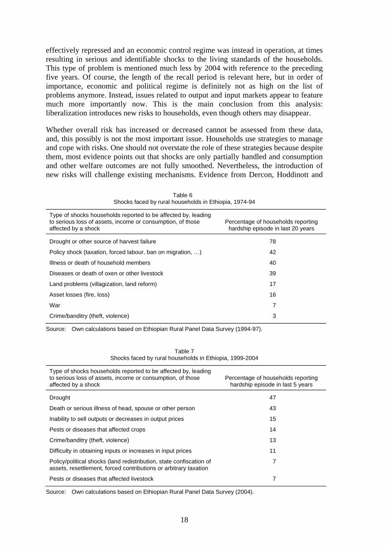
Assessing this ‘vulnerability to poverty’ is, however, very data intensive, and requires the calibration of outcomes in different states of the world. It typically requires the equivalent of a forecasting model of consumption or another dimension of wellbeing, not just of the household mean of consumption but also its distribution. Assessing the changes in the distribution of risk after liberalization in Ethiopia is not fully possible, not least since so many other factors have changed in recent years (including regionalization, a war with Eritrea, and vast market distorting aid flows). Consequently, the calibration of a counterfactual risk-due-to-liberalization distribution was not feasible. Instead, we only present some suggestive evidence on the risks faced by households, and the implications of these. In particular, in 1995, the 1477 households in ERHS were asked to name the shocks that seriously affected their standard of living or asset position in the last 20 years, based on a long list of possible shocks. Subsequently, in 2004, the survey asked the same households to nominate the experiences related to the same set of potential shocks, but this time referring to the last five years. The question was similar, although the order of questions and the categories used were different, possibly affecting the answers. The findings were, nevertheless, very suggestive.
As Table 6 showed, besides natural and life-cycle risks (health, death), and diseases or deaths of livestock, high-frequency problems are those that relate to the economic and political regime during the period 1974 until 1991. Among problems in this category forced labour, the ban of migration, high rural taxes, as well as ones concerning the land tenure and redistribution system feature highly. Problems related to the functioning of markets were rarely if ever mentioned. The explanation is simple: markets were
18
effectively repressed and an economic control regime was instead in operation, at times resulting in serious and identifiable shocks to the living standards of the households. This type of problem is mentioned much less by 2004 with reference to the preceding five years. Of course, the length of the recall period is relevant here, but in order of importance, economic and political regime is definitely not as high on the list of problems anymore. Instead, issues related to output and input markets appear to feature much more importantly now. This is the main conclusion from this analysis: liberalization introduces new risks to households, even though others may disappear.
Whether overall risk has increased or decreased cannot be assessed from these data, and, this possibly is not the most important issue. Households use strategies to manage and cope with risks. One should not overstate the role of these strategies because despite them, most evidence points out that shocks are only partially handled and consumption and other welfare outcomes are not fully smoothed. Nevertheless, the introduction of new risks will challenge existing mechanisms. Evidence from Dercon, Hoddinott and
Table 6 Shocks faced by rural households in Ethiopia, 1974-94
Type of shocks households reported to be affected by, leading to serious loss of assets, income or consumption, of those affected by a shock
Percentage of households reporting hardship episode in last 20 years
Drought or other source of harvest failure 78
Policy shock (taxation, forced labour, ban on migration, …) 42
Illness or death of household members 40
Diseases or death of oxen or other livestock 39
Land problems (villagization, land reform) 17
Asset losses (fire, loss) 16
War 7
Crime/banditry (theft, violence) 3
Source: Own calculations based on Ethiopian Rural Panel Data Survey (1994-97).
Table 7 Shocks faced by rural households in Ethiopia, 1999-2004
Type of shocks households reported to be affected by, leading to serious loss of assets, income or consumption, of those affected by a shock
Percentage of households reporting hardship episode in last 5 years
Drought 47
Death or serious illness of head, spouse or other person 43
Inability to sell outputs or decreases in output prices 15
Pests or diseases that affected crops 14
Crime/banditry (theft, violence) 13
Difficulty in obtaining inputs or increases in input prices 11
Policy/political shocks (land redistribution, state confiscation of assets, resettlement, forced contributions or arbitrary taxation
7
Pests or diseases that affected livestock 7
Source: Own calculations based on Ethiopian Rural Panel Data Survey (2004).
19
Woldehanna (2005) suggests that these new risks are significant in affecting consumption outcomes. Table 8 demonstrates this, using the outcomes of regressing the log of consumption per capita in 2004 on a number of characteristics in 1999, and shock variables based on the same questions as in Table 7. Besides the more ‘standard’ shocks, such as those related to the drought in 2002 and illness shocks, the other two shocks that show up significantly relate to the inability to sell output or a collapse of output prices, and a failing demand for non-agricultural products in a particular period. These shocks appear to reduce consumption in 2004 by 15-20 per cent, compared to what it would have been without the shocks; this is clearly a large impact.9 In sum, this is suggestive evidence that shifting risks towards market-related risks may not have suitable responses, thereby suggesting a possible further effect from liberalization policies, at least in the medium run.
Table 8 Impact of shocks on (log) consumption per capita, 2004
Estimated coefficient
t statistic (absolute
value)
Drought, 2002-04 -0.163 2.46** Drought, 1999-2001 -0.137 2.72** Pests or diseases that affected crops, 2002-04 -0.006 0.07 Pests or diseases that affected crops, 1999-2001 -0.052 1.05 Pests or diseases that affected livestock, 2002-04 -0.002 0.18 Pests or diseases that affected livestock, 1999-2001 0.022 0.24 Difficulty in obtaining inputs or increases in input prices, 2002-04 0.055 0.63 Difficulty in obtaining inputs or increases in input prices, 1999-2001 0.001 0.02 Inability to sell outputs or decreases in output prices, 2002-04 -0.187 2.23** Inability to sell outputs or decreases in output prices, 1999-2001 -0.026 0.36 Lack of demand for non-agricultural products, 2002-04 -0.037 0.19 Lack of demand for non-agricultural products, 1999-2001 -0.195 2.28** Crime shocks, 2002-04 -0.018 0.36 Crime shocks, 1999-2001 0.083 0.99 Death of head, spouse or another person, 2002-04 0.043 0.69 Death of head, spouse or another person, 1999-2001 -0.001 0.02 Illness of head, spouse or another person, 2002-04 -0.019 0.32 Illness of head, spouse or another person, 1999-2001 -0.151 2.33** R2 0.34
Sample size 1,290
Notes: Specification includes controls for Female headship, age head, schooling, household size, dependency ratio, land holdings (quintiles), livestock, ethnic minority, religious minority, holding official position in Peasant Association or important place in social life, all in 1999. PA dummies, month of interview dummies and perceptions of rainfall in previous harvest year are also included but not reported.
Standard errors are robust to locality cluster effects. * Significant at the 10% level; ** significant at the 5% level.
Source: ERHS (1999-2004), and Dercon, Hoddinott and Woldehanna (2005).
9 Of course, this regression may suffer from missing variable bias, such as those reporting these shocks
may have other unobservable characteristics. Since this regression could not be estimated with household fixed effects, there is no obvious way to control for these characteristics, besides entering observable characteristics as well did.
20
Conclusion
There is a close correlation between the role of trade in GDP, overall growth and poverty reduction in developing countries. Growth and poverty reduction have accelerated in those economies that have successfully increased their trade share in income. However, whether there is a direct causal link between trade policy, growth and poverty reduction is still disputed. Still, the substantial poverty reductions in some developing countries, such as China and, more recently, parts of India are beyond doubt.
However, for many other developing countries, globalization is still far removed. In fact, there are concerns that these countries may well become further marginalized. The reasons include poor policy environment but also poor geographical endowments. It will be a difficult task to stop this process of marginalization, not least since there are risks that these economies may get trapped in permanently low growth and high poverty due to the externalities related to globalization and marginalization. Concerted efforts within these countries with substantial outside support are likely to be needed to improve the investment climate in these economies.
There is some evidence that particular groups and areas may also risk becoming marginalized within the globalizing economies. High growth may provide the means to prevent this process from becoming self-perpetuating, but in any case action would be needed. The factors correlated with this marginalization are typically poor local endowments in terms of geography and infrastructure, as well as poor household endowments in terms of labour and assets. In many ways, the factors causing marginalization on the global scale are similar to the factors causing within-country marginalization.
These insights were illustrated using Ethiopia as a case study. Ethiopia has started a process of market and international trade liberalization, but definitely still belongs to the group of ‘marginalized’ economies in the world. Growth remains limited, and poverty is highly persistent. The welfare impact of the domestic market liberalization in the first part of the 1990s also illustrates the risks related to further marginalization of some of the poor in Ethiopia. While one substantial group of the poor has been able to take advantage of the recent improved economic environment, another group seems to have become increasingly marginalized. Investment in infrastructure provides one useful strategy to overcome some of the inherent marginal endowments in terms of infrastructure and other assets. The evidence from the 1990s from Ethiopia reported in this paper suggests that improving infrastructure had very substantial growth effects. In any case, geographic diversity in these infrastructural investments seems to be correlated with differential growth experience, suggesting that more marginal areas within Ethiopia are at risk of becoming even more marginalized during the age of globalization.
One should also realize that liberalization and more market orientation will bring other risks, which households have to find ways of coping with. Evidence from self-reported shocks suggests that market related risks (in the form of failing demand or price shocks) are more common now than they were before liberalization. This does not have to be a fundamental problem, since other risks (such as locally covariate risks) may be better spread across geographical areas. Nevertheless, it points to the need for other instruments, including those available to households, to cope with these emerging risks.
21
References
Calvo, C., and S. Dercon (2005). ‘Measuring Individual Vulnerability’. Economics Series Working Paper 229. Oxford: Department of Economics, University of Oxford.
Collier, P., and J. W. Gunning (1999). ‘Explaining African Economic Performance’. Journal of Economic Literature, 37 (March): 64-111.
Collier, P., A. Hoeffler, and C. Pattillo (2001). ‘Flight Capital as a Portfolio Choice’. The World Bank Economic Review, 15 (1): 55-80.
Dercon, S. (1995). ‘On Market Integration and Liberalization: Method and Application to Ethiopia’. Journal of Development Studies, 32 (1): 112-43.
Dercon, S. (2002). ‘The Impact of Economic Reform on Households in Rural Ethiopia 1989-95’. Washington, DC: World Bank.
Dercon, S. (2004). ‘Growth and Risk: Evidence from Rural Ethiopia’. Journal of Development Economics, 74 (2): 309-29.
Dercon, S. (2006). ‘Economic Reform, Growth and the Poor in Rural Ethiopia’. Journal of Development Economics, 81 (1): 1-24.
Dercon, S., and J. Hoddinott (2005). ‘Livelihoods, Growth and Links to Market Towns in 15 Ethiopian Villages. Washington, DC: IFPRI. Mimeo.
Dercon, S., and P. Krishnan (2002). ‘Changes in Poverty in Villages in Rural Ethiopia: 1989-95’. In A. Booth and P. Mosley (eds), The New Poverty Strategies: What Have They Achieved? What Have We Learned? Basingstoke: Macmillan.
Dercon, S., J. Hoddinott, and T. Woldehanna (2005). ‘Shocks and Consumption in 15 Villages in Rural Ethiopia’. Journal of African Economies, 14 (4): 559-85.
Dollar, D. (1992). ‘Outward Oriented Developing Countries Really Do Grow More Rapidly: Evidence from 95 LDCs, 1976-85’. Economic Development and Cultural Change, 40 (3): 523-44.
Dollar, D., and A. Kraay (2001). ‘Growth is Good for the Poor. WB Policy Research Working Paper 2587. Washington, DC. World Bank.
Oxfam (2000). ‘Globalisation, Submission to the Government’s White Paper on Globalisation’. Oxfam Policy Papers 5/00. Fitzroy: Oxfam.
Ravallion, M. (2003). The Debate on Globalization, Poverty and Inequality: Why Measurement Matters’. WB Policy Research Working Paper 3058. Washington, DC: World Bank.
Rodriguez, F., and D. Rodrik (1999). ‘Trade Policy and Economic Growth: A Skeptic’s Guide to the Cross-National Evidence’. NBER Working Paper 7081. Cambridge, MA: National Bureau of Economic Research.
Sachs, J. D., and A. Warner (1995). ‘Economic Reform and the Process of Global Integration’. Brookings Papers on Economic Activity, 1 (96): 1-118.
Winters, A., N. McCulloch, and A. McKay (2004). ‘Trade Liberalization and Poverty: The Evidence So Far’. Journal of Economic Literature, XLII (March): 72-115.
World Bank (2002). Globalization, Growth, and Poverty, Building an Inclusive World Economy. Washington, DC: World Bank.
22
Appendix: A regression based poverty decomposition
Suppose one is specifically interested in investigating the contribution to poverty changes of some variables crucial in explaining growth. We use an additive separable poverty index that is for each person linear in log consumption. The normalised poverty gap, defined over the log of consumption as the underlying welfare measure, satisfies this property.
Following Dercon (2006), formally, denote z as the log of the poverty line, yht the log of consumption of household h at t, and qt as the number of people falling below the poverty line at time t and n as the total number of individuals, which are observed over time. If one orders all individuals from poor to rich in each period, then this measure can be defined as:
1
1 tqht
th
z yPn z=
−= ∑ (1)
Let us consider two periods of time, 0 and 1, and introduce a specific counterfactual, in which the change of consumption over time is equal to Xh. For example, this could be the change in consumption stemming from the actual change in one of the endowments (as used in the regression analysis in the main text). It is then possible to calculate the counterfactual consumption for person h, yh1
*, as:
*1 0h h hy y X= + (2)
Given this change, the number of poor will change. Let us call the actual and counterfactual number of poor in period 0 and 1, respectively, q0 and q1
*. One can then define the change in poverty between period 1 and 0 as:
01** 1 0
1 01 1
1 1 qqh h
h h
z y z yP Pn z n z= =
− −− = −∑ ∑ (3)
Let us now order the individuals, so that the poor in both periods are from h = 1,... q*11,
those moving into poverty h = q*11 + 1,…q*
01 (i.e., nonpoor in period 0 and poor in period 1), those moving out of poverty ranked h = q*
01 + 1, …q*10, and finally, those
non-poor in each period as h = q*10 + 1,…, n. Then, (3) can be written as:
* **01 0111
* *11 01
* ** 1 0 1 0
1 01 1 1
1 1 1( )q qq
h h h h
h h q i q
z y z y z y z yP Pn z z n z n z= = + = +
− − − −− = − + −∑ ∑ ∑ (4)
i.e., the change in the gap consist of the change of the gap of those poor in both periods, plus the gap of those poor in the second but not in the first period, minus the gap in the first period of those leaving poverty.10 Dividing the left- and right-hand side of (4) by
10 As suggested earlier and using the notation as before, the Watts poverty measure is defined as:
1
1 tq
t hth
W z yn =
= −∑
so that the decomposition is effectively a decomposition of the Watts poverty measure. Just as the squared poverty gap, it is convex in levels of consumption, implying that consumption levels far
23
(P1*–P0) yields a decomposition in terms of the contribution to the total poverty change
of those staying poor, those becoming poor and those leaving poverty. Note that this is an additive decomposition. This can be rewritten in terms of changes in consumption. The part in brackets in the first term of (4) is directly defined in terms of yh1
*– yh0 = Xh. Pre-multiplying the terms within the summation sign for each of the two subsequent terms by (yh0 – yh1
*)/(yh0 – yh1*). Slightly rewritten (4) becomes:
01 1011
11 01
* **** 1 0
1 0 * *1 * 1 * 11 1
1 1 1( ) ( )( ) ( )( )q qq
i i i i i
i i q i qio i io i
X X z y z y XP Pn z n z y y n y y z= = + = +
− − − − −− = + −− −∑ ∑ ∑ (5)
This expression suggests (rather self-evidently) that when calculating the total counterfactual poverty change, for households who leave or enter into poverty, only the consumption change up to or counting from the poverty line will be taken into account, while for those staying poor, their entire consumption change is relevant. This allows us to define the share of the consumption change that has to be taken into account as:
* 1hs = for qh ∈ {1,…q11*}, (6a)
** 1
*0 1
hh
h h
z ysy y
−=−
for qh ∈ {q11*+1,…,q01
*} and (6b)
* 0*1 0
hh
h h
z ysy y
−=−
for qh ∈ {q01* +1,…,q10
*} (6c)
Note that these shares sh* are dependent on the specific counterfactual studied, and between zero and one.
Using (6a), (6b) and (6c), (5) can be rewritten as:
*10
* *1 0
1
1 ( )q
hh
h
XP P sn z=
−− = ∑ (7)
Equation (7) may seem only of limited interest: if only one factor is considered in the counterfactual, the equation only describes what in practice is calculated via simulations. Calculating the weights sh* is probably more time-consuming than calculating the change in poverty directly from the derived and the actual distribution. Furthermore, (7) is restricted to very specific poverty measures, while micro-simulations can handle any measure. Nevertheless, (7) becomes more interesting when X is itself determined by different variables.
First, let us consider a case in which the counterfactual consists of two parts (V and W), and assume that for each h, Xh =Vh + Wh. Now (7) can be used to study the contribution
below the poverty line have a higher weight than levels closer to the poverty line, unlike the poverty gap, which is linear in levels of consumption.
24
of each factor Vh and Wh in the total counterfactual change. For a given total change in consumption, the shares sh* will be constant, so that (7) can be written as:
* *10 10
* * *1 0
1 1
1 1( ) ( )q q
h hh h
h h
V WP P s sn z n z= =
− −− = +∑ ∑ (8)
This implies that, for a given total change, the contribution of different factors to the change in poverty can be directly derived from (8). Note that these contributions sum to one, but also that they are always defined relative to a particular total counterfactual change. For example, let us define P1
V (P1W) as poverty in period 1 when V (W) has
been added to yh0. Even though (yh0 + Xh) = (yh0 + Vh + Wh), it can be easily seen that
*1 0 1 0 1 0( ) ( )V WP P P P P P− ≠ − + − .
In other words, the total poverty change due to adding both V and W to consumption is not simply equal to the poverty change induced by adding V and W separately. This means that the decomposition has to be carefully interpreted. Equation (8) can be easily generalised to more factors, it will be used below to interpret the contribution to poverty changes of different factors linked to economic reform.
One counterfactual is of particular interest for the current research: assessing the contribution of different factors to the actual observed total change in poverty (P1–P0). With an appropriate residual term (εh), Equation (1) provides a prediction model for changes in consumption for each person, based on different factors. Or, more in general, suppose Xh = Vh + Wh + εh. Equation (8) can then be rewritten as (dropping asterisks, since the counterfactual considered is the actual change in poverty):
10 10 10
1 01 1 1
1 1 1( ) ( ) ( )q q q
h h hh h h
h h h
V WP P s s sn z n z n z
ε= = =
− − −− = + +∑ ∑ ∑ (9)
Equation (9) provide then simple ways of describing the contribution of these different factors (and the error term) to the observed poverty changes, using shares sh based on the actual observed poverty transitions. It shows a direct link between changes in individual consumption over time and the poverty outcome. The overall result is a decomposition of the poverty gap into the effects of changes in fixed endowments, changes in input and output prices, and random events, for a given total change in poverty. The decomposition will now be applied to data related to 1989 and 1994/5, before and after a major set of reform measures was implemented. The decomposition of consumption changes is exact when using an estimation method which impose that that the sum of the residuals is zero, such as OLS. Decompositions based on (9) are additive in terms of the contributing factors but not exact and the contribution of the error term will have to be added.