Resilient Modulus for New Hampshire Subgrade Soils for … · Resilient Modulus for New Hampshire...

Resilient Modulus for New HampshireSubgrade Soils for Use inMechanistic AASHTO Design

SPEC

IAL

REP

OR

T

99-

14

Vincent C. Janoo, John J. Bayer Jr., Glenn D. Durell, September 1999and Charles E. Smith Jr.

US Army Corpsof Engineers®

Cold Regions Research &Engineering Laboratory

Abstract: Resilient modulus tests were conducted on fivesubgrade soils commonly found in the state of NewHampshire. Tests were conducted on samples preparedat optimum density and moisture content. To determinethe effective resilient modulus of the various soils fordesign purposes, tests were conducted at room tem-

How to get copies of CRREL technical publications:

Department of Defense personnel and contractors may order reports through the Defense Technical Information Center:DTIC-BR SUITE 09448725 JOHN J KINGMAN RDFT BELVOIR VA 22060-6218Telephone 1 800 225 3842E-mail [email protected]

[email protected] http://www.dtic.dla.mil/

All others may order reports through the National Technical Information Service:NTIS5285 PORT ROYAL RDSPRINGFIELD VA 22161Telephone 1 800 553 6847 or 1 703 605 6000

1 703 487 4639 (TDD for the hearing-impaired)E-mail [email protected] http://www.ntis.gov/index.html

A complete list of all CRREL technical publications is available from:USACRREL (CEERD-IM-HL)72 LYME RDHANOVER NH 03755-1290Telephone 1 603 646 4338E-mail [email protected]

For information on all aspects of the Cold Regions Research and Engineering Laboratory, visit our World Wide Web site:http://www.crrel.usace.army.mil

perature and at freezing temperatures. The AASHTO TP46 test protocol was used for testing room temperatureand thawing soils. At freezing temperatures, the CRRELtest protocol was used. The results from this test pro-gram are presented in this report. In addition, suggestedeffective resilient modulus for the five soils are presented.

Resilient Modulus for New HampshireSubgrade Soils for Use inMechanistic AASHTO Design

Special Report 99-14

Vincent C. Janoo, John J. Bayer Jr., Glenn D. Durell, September 1999and Charles E. Smith Jr.

Prepared for

OFFICE OF THE CHIEF OF ENGINEERS

Approved for public release; distribution is unlimited.

US Army Corpsof Engineers®

Cold Regions Research &Engineering Laboratory

PREFACE

This report was prepared by Dr. Vincent C. Janoo, Research Civil Engineer, andJohn J. Bayer Jr., Glenn D. Durell, and Charles E. Smith Jr., Engineering Techni-cians, of the Civil Engineering Research Division, U.S. Army Cold Regions Researchand Engineering Laboratory (CRREL), Hanover, New Hampshire.

This work was funded through an Intergovernmental Cooperative Agreement(ICA) between the State of New Hampshire, Department of Transportation(NHDOT), and CRREL. This work has been designated as NHDOT Statewide Project12323P.

The authors thank Glenn Roberts, NHDOT, and Sally Shoop, CRREL, for techni-cally reviewing the manuscript of this report. Thomas Clearly and Paul Matthewsof NHDOT and David Hall of FHWA contributed significantly to this review. Theauthors also thank Lynette Barna for assisting in organizing the report, and EdmundWright and John Severance for editing and getting the report in its final form. Lastbut not least, special thanks are due to Dawn Boden and Jane Mason for the illus-trations.

This report was prepared in cooperation with the New Hampshire Departmentof Transportation and the U.S. Department of Transportation, Federal HighwayAdministration.

The contents of this report reflect the views of the authors who are responsiblefor the facts and the accuracy of the data presented herein. The contents do notnecessarily reflect the official views of policies of the New Hampshire Departmentof Transportation or the Federal Highway Administration at the time of publica-tion. This report does not constitute a standard, specification, or regulation.

The contents of this report are not to be used for advertising or promotionalpurposes. Citation of brand names does not constitute an official endorsement orapproval of the use of such commercial products.

ii

iii

CONTENTS

Preface .......................................................................................................................... iiExecutive summary .................................................................................................... vIntroduction ................................................................................................................. 1Description of test soils .............................................................................................. 3Test program ................................................................................................................ 3Results and discussion ............................................................................................... 5Recommendations/conclusions ............................................................................... 23Literature cited ............................................................................................................ 24Appendix A: Uniform density and moisture content ........................................... 25Appendix B: Sample preparation/testing............................................................... 30Abstract ........................................................................................................................ 35

ILLUSTRATIONS

Figure1. Chart for estimating effective roadbed soil resilient modulus

for flexible pavement designed using the serviceability criteria ............. 22. Grain size distribution for test soils ................................................................... 33. Kneading compactor used for fabricating test specimens .............................. 44. Typical sample setup ............................................................................................ 55. Effect of freezing and thawing on the resilient modulus of silty

glacial till .......................................................................................................... 146. Effect of freezing and thawing on the resilient modulus of coarse

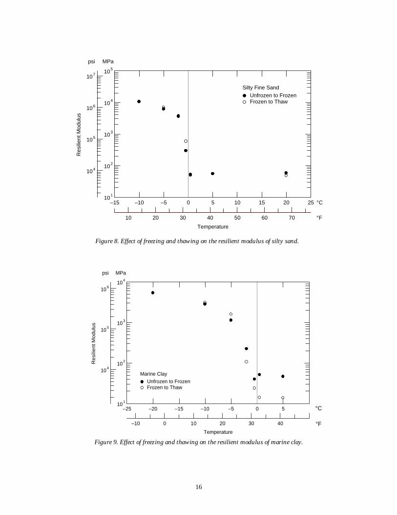
gravelly sand ................................................................................................... 157. Effect of freezing and thawing on the resilient modulus of fine sand .......... 158. Effect of freezing and thawing on the resilient modulus of silty sand ......... 169. Effect of freezing and thawing on the resilient modulus of marine clay ..... 16

10. Typical pavement cross sections used by NHDOT ......................................... 1711. Design air temperatures used for estimating subgrade temperatures ......... 1712. Annual temperature at the top of the subgrade (interstate pavement

system), Concord, New Hampshire ............................................................. 1813. Annual temperature at the top of the subgrade (secondary pavement

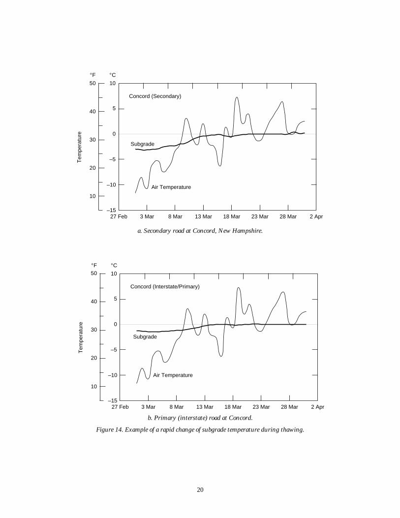
system), Concord, New Hampshire ............................................................. 1814. Example of a rapid change of subgrade temperature during thawing ........ 20

TABLES

Table1. Classification properties of test soils .................................................................. 42. Testing sequence protocol used in the resilient modulus test ........................ 53. Test conditions and types of tests ....................................................................... 64. Test temperatures for shear tests ........................................................................ 65. Test temperatures for hydrostatic compression tests ...................................... 66. Resilient modulus test results for NH1 ............................................................. 77. Resilient modulus test results for NH2 ............................................................. 8

iv

Table8. Resilient modulus test results for NH3 ............................................................. 109. Resilient modulus test results for NH4 ............................................................. 12

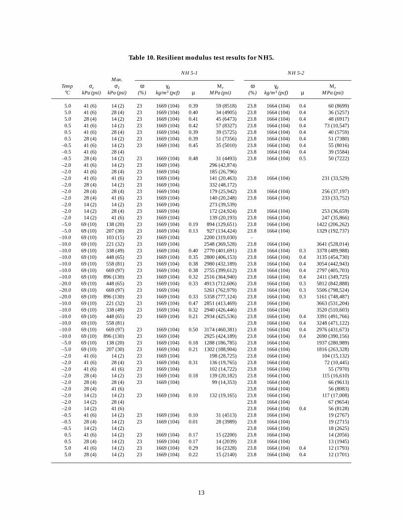
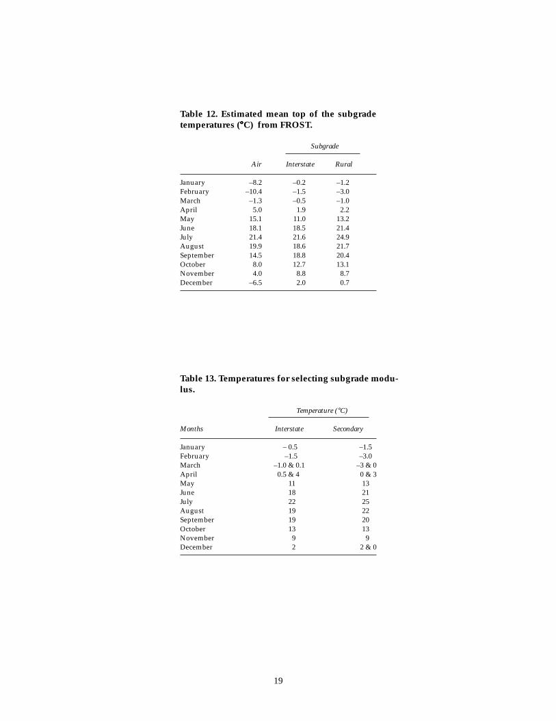
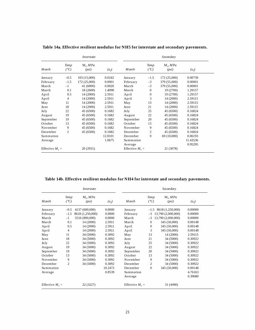
10. Resilient modulus test results for NH5 ............................................................. 1311. Average resilient modulus of subgrade soils as a function of temperature . 1412. Estimated mean top of the subgrade temperatures (°C) from FROST ........ 1913. Temperatures for selecting subgrade modulus ................................................ 1914. Effective resilient modulus for NH 5 for interstate and secondary

pavements ........................................................................................................ 2115. Summary of effective resilient modulus for NH subgrade soils ................... 2316. Recommended effective moduli for subgrade soils ........................................ 23

EXECUTIVE SUMMARY

Resilient modulus tests were conducted on five subgrade soils considered to berepresentative of the subgrade soils found in the state of New Hampshire. Testswere conducted at the optimum density and moisture content. The optimum den-sity and moisture content for the five soils were provided by the New HampshireDepartment of Transportation (NHDOT). Although the focus was on resilient modu-lus tests, a limited number of hydrostatic and triaxial compression tests were con-ducted.

The tests were conducted to determine the effective resilient modulus of thesoils for use in the AASHTO design procedure. Resilient modulus tests were con-ducted at several temperatures to reflect freezing and thawing. Temperature wasselected as the primary variable because it is the easiest to measure in the field. Thetests were conducted using the AASHTO TP 46 test protocol, except when thesamples were frozen. When frozen, the CRREL testing protocols was used. Althoughtests were done at different confining pressures and deviator stress, the averagevalues were used to determine the effective modulus. This is justifiable, as theAASHTO design method requires a single resilient modulus value. These valuescan be used with most mechanistic design methods as they use linear elastic prop-erties. However, the nonlinear information is available in this report for future non-linear analysis. A limited number of radial strain measurements were made, andPoisson’s ratio was calculated. Many of these values were outside the conventionalrange of Poisson’s ratio for elastic materials. This is to be expected since subgradesoils are not linear homogenous material but a conglomeration of aggregates orparticles.

Samples were prepared using a kneading compactor. A series of tests were con-ducted to determine the correct kneading pressure and the number of tamps toprovide a uniform density (as a function of depth) for the sample at the optimummoisture content.

The computer program FROST was used to determine the temperature at top ofthe subgrade for typical interstate and rural pavements. Temperatures for both theConcord and Lebanon, New Hampshire, areas were used in the analysis. It wasfound that the subgrade temperatures were similar at Concord and Lebanon. Theresults presented here are for Concord but can be used in most of the state. Theexception may be in high areas at higher elevations. The monthly resilient modu-lus selected was based on the subgrade temperatures, not on the mean air tempera-tures. The effective resilient modulus for the five soils for each month of the yearare presented in the recommendation/conclusion sections. The results presentedin this report are for optimum density moisture conditions. Care must be takenwith its use at other densities or moisture conditions.

v

Resilient Modulus for New HampshireSubgrade Soils for Use in

Mechanistic AASHTO Design

VINCENT C. JANOO, JOHN J. BAYER JR., GLENN D. DURELL, AND CHARLES E. SMITH JR.

INTRODUCTION

The American Association of State Highwayand Transportation Officials (AASHTO) pavementdesign procedure is an empirical design methodbased on the results from the AASHO road tests.The AASHO (the precursor of AASHTO) road testswere conducted near Ottawa, Illinois, around 1958to 1960. The road tests were conducted on asphaltconcrete pavements, portland cement concretepavements, and bridge decks. A total of 10lanes were tested under controlled loading rangingfrom 9-kN (2,000-lbf) single axle loads to 215-kN(48,000-lbf) tandem axle loads. A total of 1,114,000axle loads were applied during the road test.

The design is based on the functional proper-ties of the pavement structure, such as cracking,rutting, and roughness. This change in the func-tional properties is indexed by the present service-ability index (PSI). The PSI ranges from 0 to 5, with5 designating excellent conditions. On highwaypavement, when the PSI has reached 2.5, majorrehabilitation is required. The original design, eq1, is a relationship between 80-kN (18-kip) axleloads to thickness of the pavement layers and thesubgrade at the AASHO road tests:

log . log( ) .W SNt18 9 36 1 0 20= + −

log ( . )/( . . )

. /( ) .

p

SN

t5 19

4 2 4 2 1 5

0 40 1094 1+

− −[ ]+ +[ ] (1)

where Wt18 = 80-kN total load application at endof time t,

SN = structural number of pavement,pt = terminal serviceability index.

Later, eq 1 was modified to account forsubgrade soil types other than the type A-6found at the AASHO Test Road. A soil supportterm (Si) was added to eq 1 and is shown ineq 2:

log . log .W SNt18 9 36 1 0 20= +( ) −

log . / . .

. / .

p

SN

t5 19

4 2 4 2 1 5

0 40 1094 1+

−( ) −( )[ ]+ +( )[ ]

log . .R

Si1

0 372 3 0+ + −( ) . (2)

Si for the AASHO subgrade soil was set at 3.0,and Si can range between 3 and 10, with 10 repre-senting a crushed rock type subgrade. R is a re-gional factor introduced to account for climatesother than Ottawa, Illinois.

With the introduction of the AASHTO 1996 de-sign guide (AASHTO 1996a), the soil supportvalue was replaced by the effective resilient modu-lus Mr of the subgrade soil:

log . log .W SNt18 9 36 1 0 20= +( ) − +

log . / . .

. / .

p

SN

t5 19

4 2 4 2 1 5

0 40 1094 1+

−( ) −( )[ ]+ +( )[ ]

. log .Mr2 32 8 07+ − . (3)

2

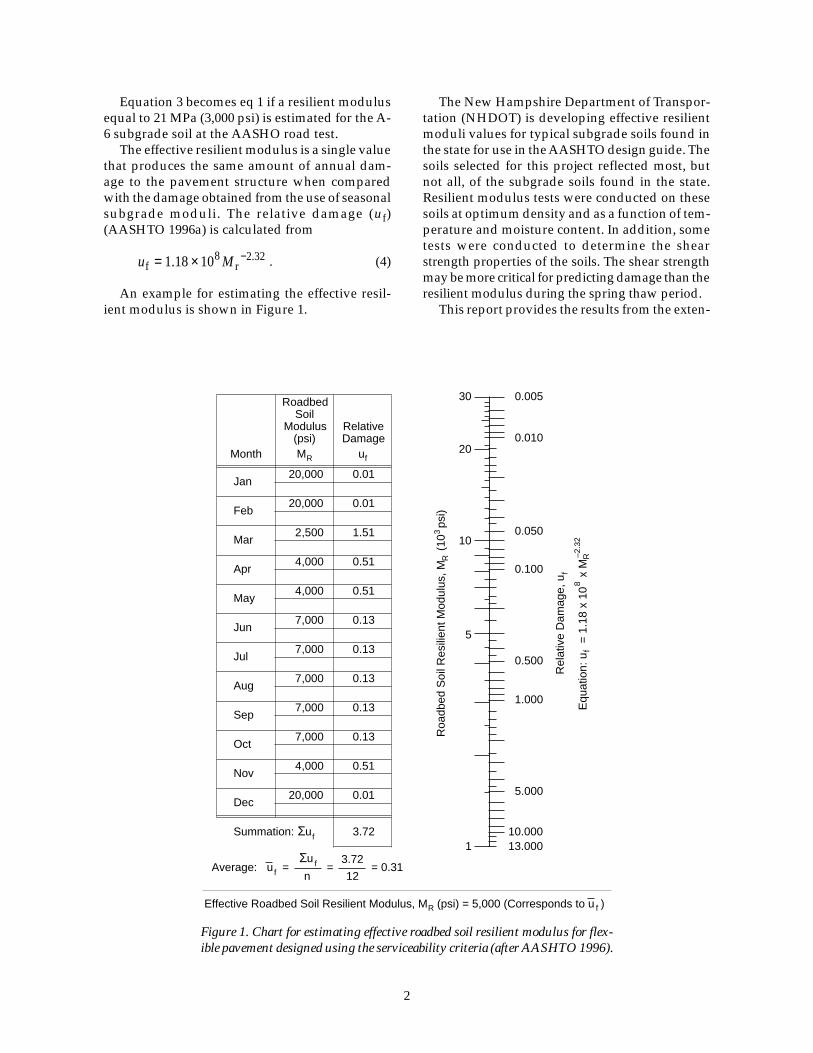
Equation 3 becomes eq 1 if a resilient modulusequal to 21 MPa (3,000 psi) is estimated for the A-6 subgrade soil at the AASHO road test.

The effective resilient modulus is a single valuethat produces the same amount of annual dam-age to the pavement structure when comparedwith the damage obtained from the use of seasonalsubgrade moduli. The relative damage (uf)(AASHTO 1996a) is calculated from

u Mf r= × −1 18 108 2 32. . . (4)

An example for estimating the effective resil-ient modulus is shown in Figure 1.

The New Hampshire Department of Transpor-tation (NHDOT) is developing effective resilientmoduli values for typical subgrade soils found inthe state for use in the AASHTO design guide. Thesoils selected for this project reflected most, butnot all, of the subgrade soils found in the state.Resilient modulus tests were conducted on thesesoils at optimum density and as a function of tem-perature and moisture content. In addition, sometests were conducted to determine the shearstrength properties of the soils. The shear strengthmay be more critical for predicting damage than theresilient modulus during the spring thaw period.

This report provides the results from the exten-

ufAverage: = = = 0.31Σu f

n 12

3.72

Feb

Jan

Mar

Apr

May

Jun

Jul

Aug

Sep

Oct

Nov

Dec

20,000

20,000

20,000

2,500

4,000

7,000

4,000

4,000

7,000

7,000

7,000

7,000

0.01

0.01

0.01

1.51

0.51

0.13

0.51

0.51

0.13

0.13

0.13

0.13

MR uf

RoadbedSoil

Modulus(psi)

RelativeDamage

Month

3.72Summation: Σuf

Rel

ativ

e D

amag

e, u

f

30

20

10

5

1

0.005

0.010

1.000

5.000

10.00013.000

0.500

0.100

0.050

Equ

atio

n: u

=

1.1

8 x

10

x M

fR

8–2

.32

Effective Roadbed Soil Resilient Modulus, M (psi) = 5,000 (Corresponds to u ) R f

Roa

dbed

Soi

l Res

ilien

t Mod

ulus

, M

(10

psi

)3

R

Figure 1. Chart for estimating effective roadbed soil resilient modulus for flex-ible pavement designed using the serviceability criteria (after AASHTO 1996).

3

sive laboratory testing to determine the resilientmodulus of the various subgrade soils as a func-tion of temperature. It also provides a guide forselecting the appropriate resilient modulus valuesto be used in the current AASHTO design method.These values can also be used in future modifica-tions to the AASHTO design method as proposedin the current AASHTO 2002 design guide researchstudy.

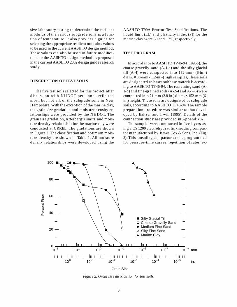
DESCRIPTION OF TEST SOILS

The five test soils selected for this project, afterdiscussion with NHDOT personnel, reflectedmost, but not all, of the subgrade soils in NewHampshire. With the exception of the marine clay,the grain size gradation and moisture density re-lationships were provided by the NHDOT. Thegrain size gradation, Atterberg’s limits, and mois-ture density relationship for the marine clay wereconducted at CRREL. The gradations are shownin Figure 2. The classification and optimum mois-ture density are shown in Table 1. All moisturedensity relationships were developed using the

AASHTO T99A Proctor Test Specifications. Theliquid limit (LL) and plasticity index (PI) for themarine clay were 50 and 17%, respectively.

TEST PROGRAM

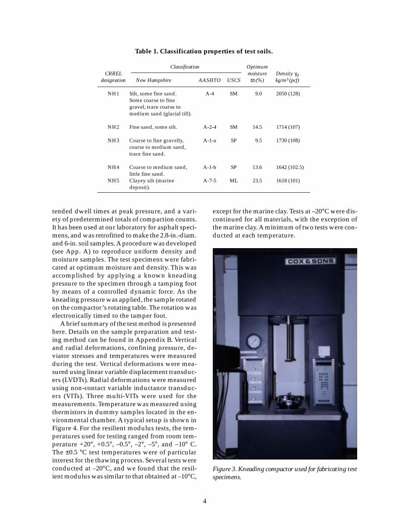
In accordance to AASHTO TP46-94 (1996b), thecoarse gravelly sand (A-1-a) and the silty glacialtill (A-4) were compacted into 152-mm- (6-in.-)diam. × 30-mm- (12-in.-) high samples, These soilsare designated as base/subbase materials accord-ing to AASHTO TP46-94. The remaining sand (A-1-b) and fine-grained soils (A-2-4 and A-7-5) werecompacted into 71-mm (2.8-in.) diam. × 152-mm (6-in.) height. These soils are designated as subgradesoils, according to AASHTO TP46-94. The samplepreparation procedure was similar to that devel-oped by Baltzer and Irwin (1995). Details of thecompaction study are provided in Appendix A.

The samples were compacted in five layers us-ing a CS 1200 electrohydraulic kneading compac-tor manufactured by James Cox & Sons, Inc. (Fig.3). This kneading compactor can be programmedfor pressure–time curves, repetition of rates, ex-

100

80

60

40

20

0

Per

cent

Fin

er

102 10–4101 100 10–1 10–2 10–3 mm

Grain Size

100 10–1 10–2 10–3 10–4 10–5 in.

Silty Glacial Till

Silty Fine SandMedium Fine SandCoarse Gravelly Sand

Marine Clay

Figure 2. Grain size distribution for test soils.

4

tended dwell times at peak pressure, and a vari-ety of predetermined totals of compaction counts.It has been used at our laboratory for asphalt speci-mens, and was retrofitted to make the 2.8-in.-diam.and 6-in. soil samples. A procedure was developed(see App. A) to reproduce uniform density andmoisture samples. The test specimens were fabri-cated at optimum moisture and density. This wasaccomplished by applying a known kneadingpressure to the specimen through a tamping footby means of a controlled dynamic force. As thekneading pressure was applied, the sample rotatedon the compactor’s rotating table. The rotation waselectronically timed to the tamper foot.

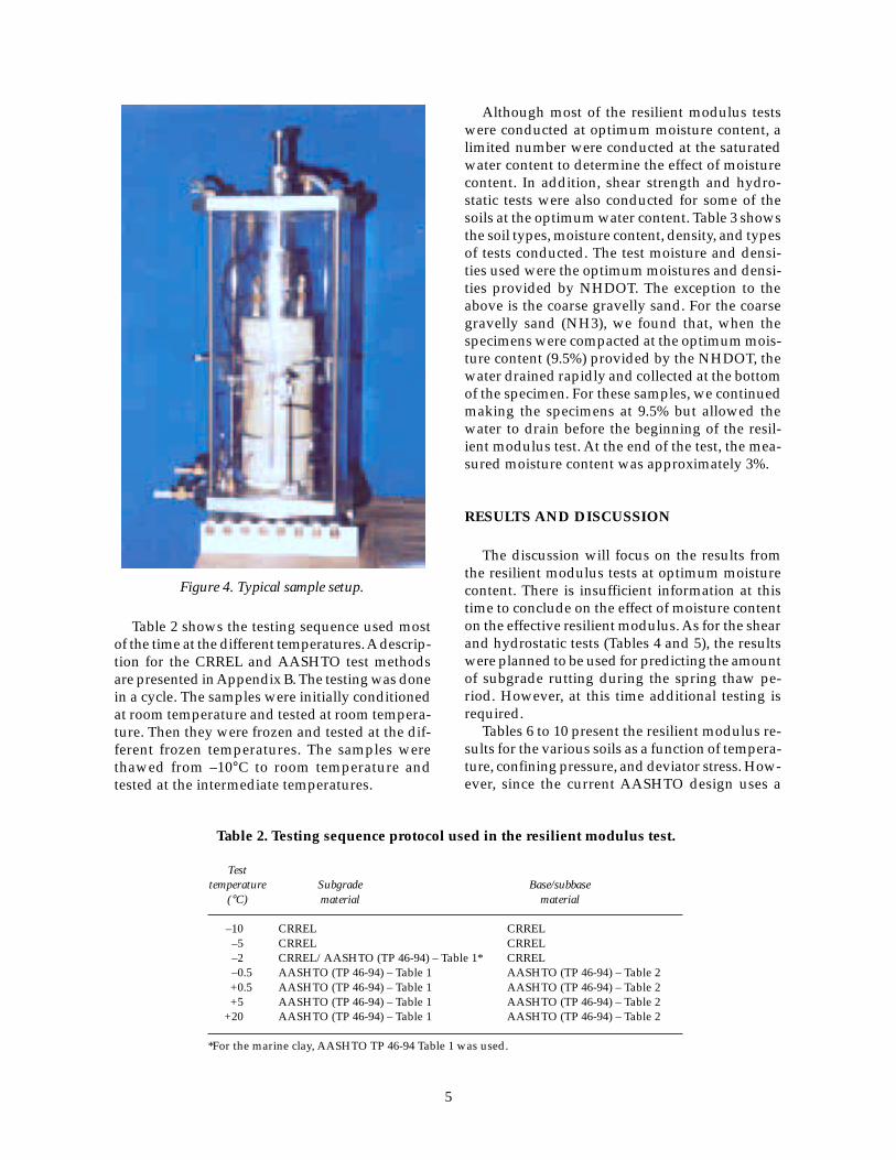
A brief summary of the test method is presentedhere. Details on the sample preparation and test-ing method can be found in Appendix B. Verticaland radial deformations, confining pressure, de-viator stresses and temperatures were measuredduring the test. Vertical deformations were mea-sured using linear variable displacement transduc-ers (LVDTs). Radial deformations were measuredusing non-contact variable inductance transduc-ers (VITs). Three multi-VITs were used for themeasurements. Temperature was measured usingthermistors in dummy samples located in the en-vironmental chamber. A typical setup is shown inFigure 4. For the resilient modulus tests, the tem-peratures used for testing ranged from room tem-perature +20°, +0.5°, –0.5°, –2°, –5°, and –10° C.The ±0.5 °C test temperatures were of particularinterest for the thawing process. Several tests wereconducted at –20°C, and we found that the resil-ient modulus was similar to that obtained at –10°C,

Table 1. Classification properties of test soils.

Classification OptimumCRREL moisture Density γd

designation New Hampshire AASHTO USCS ω (%) kg/m3 (pcf)

NH1 Silt, some fine sand. A-4 SM 9.0 2050 (128)Some coarse to finegravel, trace coarse tomedium sand (glacial till).

NH2 Fine sand, some silt. A-2-4 SM 14.5 1714 (107)

NH3 Coarse to fine gravelly, A-1-a SP 9.5 1730 (108)coarse to medium sand,trace fine sand.

NH4 Coarse to medium sand, A-1-b SP 13.6 1642 (102.5)little fine sand.

NH5 Clayey silt (marine A-7-5 ML 23.5 1618 (101)deposit).

Figure 3. Kneading compactor used for fabricating testspecimens.

except for the marine clay. Tests at –20°C were dis-continued for all materials, with the exception ofthe marine clay. A minimum of two tests were con-ducted at each temperature.

5

Table 2 shows the testing sequence used mostof the time at the different temperatures. A descrip-tion for the CRREL and AASHTO test methodsare presented in Appendix B. The testing was donein a cycle. The samples were initially conditionedat room temperature and tested at room tempera-ture. Then they were frozen and tested at the dif-ferent frozen temperatures. The samples werethawed from –10°C to room temperature andtested at the intermediate temperatures.

Although most of the resilient modulus testswere conducted at optimum moisture content, alimited number were conducted at the saturatedwater content to determine the effect of moisturecontent. In addition, shear strength and hydro-static tests were also conducted for some of thesoils at the optimum water content. Table 3 showsthe soil types, moisture content, density, and typesof tests conducted. The test moisture and densi-ties used were the optimum moistures and densi-ties provided by NHDOT. The exception to theabove is the coarse gravelly sand. For the coarsegravelly sand (NH3), we found that, when thespecimens were compacted at the optimum mois-ture content (9.5%) provided by the NHDOT, thewater drained rapidly and collected at the bottomof the specimen. For these samples, we continuedmaking the specimens at 9.5% but allowed thewater to drain before the beginning of the resil-ient modulus test. At the end of the test, the mea-sured moisture content was approximately 3%.

RESULTS AND DISCUSSION

The discussion will focus on the results fromthe resilient modulus tests at optimum moisturecontent. There is insufficient information at thistime to conclude on the effect of moisture contenton the effective resilient modulus. As for the shearand hydrostatic tests (Tables 4 and 5), the resultswere planned to be used for predicting the amountof subgrade rutting during the spring thaw pe-riod. However, at this time additional testing isrequired.

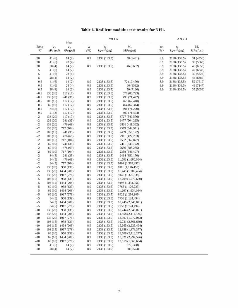
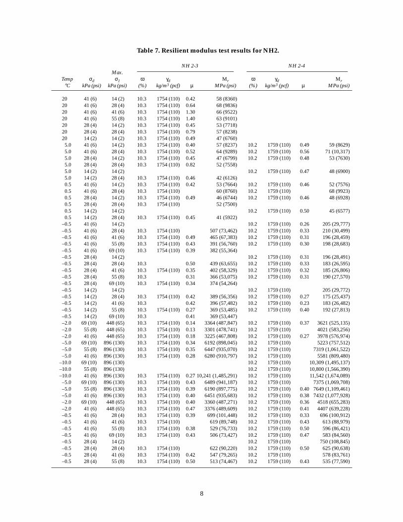
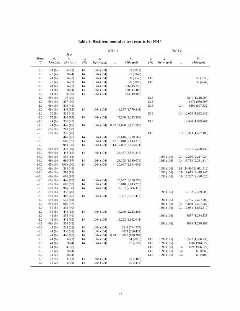
Tables 6 to 10 present the resilient modulus re-sults for the various soils as a function of tempera-ture, confining pressure, and deviator stress. How-ever, since the current AASHTO design uses a

Table 2. Testing sequence protocol used in the resilient modulus test.

Testtemperature Subgrade Base/subbase

(°C) material material

–10 CRREL CRREL–5 CRREL CRREL–2 CRREL/AASHTO (TP 46-94) – Table 1* CRREL–0.5 AASHTO (TP 46-94) – Table 1 AASHTO (TP 46-94) – Table 2+0.5 AASHTO (TP 46-94) – Table 1 AASHTO (TP 46-94) – Table 2+5 AASHTO (TP 46-94) – Table 1 AASHTO (TP 46-94) – Table 2

+20 AASHTO (TP 46-94) – Table 1 AASHTO (TP 46-94) – Table 2

*For the marine clay, AASHTO TP 46-94 Table 1 was used.

Figure 4. Typical sample setup.

6

single value to represent the resilient modulus ofthe subgrade, the test values are averaged at eachtemperature and presented in Table 11 and graphi-cally in Figures 5 to 9. Analysis of the effect of con-fining pressure, deviator stress, and temperatureon the resilient modulus is presented by Simonsenet al. (in prep.). In all cases, as expected, the resil-ient modulus increases significantly when the tem-perature drops to below freezing. Observation ofthe results indicate that the rate of change is larg-est between 0° and –2°C for all soils during freez-ing and thawing. At temperatures below –2°C, thedifference in the resilient modulus during freez-ing or thawing is minimal. However, close to 0°C,there are significant differences between themodulus obtained during the freezing and thaw-ing process. There is a significant decrease (ap-

proximately 3.5 times less) in the resilient moduliof the clay and the fine sand after thaw and beforefreezing. It also appears never to regain strength.At positive temperatures, the resilient modulusremains constant.

It is well known that during the freezing andthawing process, the ground temperatures arehigher or lower than the air temperatures. Usingthe mean air temperature to determine themonthly resilient modulus may produce signifi-cantly different moduli values. The FROST model(Guymon et al. 1993) was used to estimate the tem-perature at the top of the subgrade. The top of thesubgrade was chosen since the current mechanis-tic model use the vertical strain at top of thesubgrade as a failure criteria. Basically, the modelis a one-dimensional vertical heat mass moisture

Table 3. Test conditions and types of tests.

Test moisture/density Resilient modulusCRREL Hydrostatic

designation AASHTO ω (%) γd kg/m3 (pcf) Optimum Saturated Shear compression

NH1 A-4 9 2050 (128) √ √ √NH2 A-2-4 14.5 1714 (107) √NH3 A-1-a 9.5 1730 (108) √ √ √NH4 A-1-b 13.6 1642 (102.5) √ √ √ √NH5 A7-5 23.5 1618 (101) √

Table 5. Test temperatures for hydrostaticcompression tests.

Test temperature (°C)CRREL

designation 20 0.5 –0.5 –2

NH1 √ √NH2NH3 √NH4 √

Table 4. Test temperatures for shear tests.

Test temperature (°C)CRREL

designation 20 0.5 –0.5 –2 20T

NH1 21, 34.5, 138* 103, 138 (15,20)(3,5,20)

NH2NH3 138 (20) 138 (20) 138 (20)NH4 69 (10)

*Numbers in table are confining pressures in kPa (psi).

7

Table 6. Resilient modulus test results for NH1.

NH 1-5 NH 1-4Max.

Temp σc σ1 ω γd Mr ω γd Mr°C kPa (psi) kPa (psi) (%) kg/m3 (pcf) MPa (psi) (%) kg/m3 (pcf) MPa (psi)

20 41 (6) 14 (2) 8.9 2138 (133.5) 58 (8431) 8.9 2138 (133.5) 31 (4550)20 41 (6) 28 (4) 8.9 2138 (133.5) 39 (5665)20 28 (4) 14 (2) 8.9 2138 (133.5) 46 (6602) 8.9 2138 (133.5) 46 (6653)

5 41 (6) 14 (2) 8.9 2138 (133.5) 47 (6843)5 41 (6) 28 (4) 8.9 2138 (133.5) 39 (5623)5 28 (4) 14 (2) 8.9 2138 (133.5) 44 (6387)0.5 41 (6) 14 (2) 8.9 2138 (133.5) 72 (10,470) 8.9 2138 (133.5) 52 (7519)0.5 41 (6) 28 (4) 8.9 2138 (133.5) 66 (9532) 8.9 2138 (133.5) 49 (7147)0.5 28 (4) 14 (2) 8.9 2138 (133.5) 50 (7196) 8.9 2138 (133.5) 35 (5056)

–0.5 138 (20) 117 (17) 8.9 2138 (133.5) 577 (83,723)–0.5 138 (20) 241 (35) 8.9 2138 (133.5) 493 (71,472)–0.5 103 (15) 117 (17) 8.9 2138 (133.5) 465 (67,410)–0.5 69 (10) 117 (17) 8.9 2138 (133.5) 464 (67,314)–0.5 34 (5) 117 (17) 8.9 2138 (133.5) 491 (71,220)–0.5 21 (3) 117 (17) 8.9 2138 (133.5) 493 (71,454)–2 138 (20) 117 (17) 8.9 2138 (133.5) 3727 (540,576)–2 138 (20) 241 (35) 8.9 2138 (133.5) 3477 (504,235)–2 138 (20) 476 (69) 8.9 2138 (133.5) 2836 (411,362)–2 138 (20) 717 (104) 8.9 2138 (133.5) 2379 (344,971)–2 103 (15) 241 (35) 8.9 2138 (133.5) 2469 (358,172)–2 103 (15) 476 (69) 8.9 2138 (133.5) 2911 (422,203)–2 103 (15) 717 (104) 8.9 2138 (133.5) 2502 (362,877)–2 69 (10) 241 (35) 8.9 2138 (133.5) 2411 (349,772)–2 69 (10) 476 (69) 8.9 2138 (133.5) 2656 (385,285)–2 69 (10) 717 (104) 8.9 2138 (133.5) 2388 (346,407)–2 34 (5) 241 (35) 8.9 2138 (133.5) 2414 (350,170)–2 34 (5) 476 (69) 8.9 2138 (133.5) 11,588 (1,680,664)–2 34 (5) 717 (104) 8.9 2138 (133.5) 9404 (1,363,997)–5 138 (20) 958 (139) 8.9 2138 (133.5) 8111 (1,176,455)–5 138 (20) 1434 (208) 8.9 2138 (133.5) 11,745 (1,703,464)–5 138 (20) 1917 (278) 8.9 2138 (133.5) 9145 (1,326,338)–5 103 (15) 958 (139) 8.9 2138 (133.5) 12,209 (1,770,660)–5 103 (15) 1434 (208) 8.9 2138 (133.5) 9198 (1,334,056)–5 69 (10) 958 (139) 8.9 2138 (133.5) 7765 (1,126,223)–5 69 (10) 1434 (208) 8.9 2138 (133.5) 11,267 (1,634,094)–5 69 (10) 1917 (278) 8.9 2138 (133.5) 8922 (1,294,109)–5 34 (5) 958 (139) 8.9 2138 (133.5) 7753 (1,124,494)–5 34 (5) 1434 (208) 8.9 2138 (133.5) 18,245 (2,646,071)–5 34 (5) 1917 (278) 8.9 2138 (133.5) 7753 (1,124,494)

–10 138 (20) 958 (139) 8.9 2138 (133.5) 18,244 (2,646,071)–10 138 (20) 1434 (208) 8.9 2138 (133.5) 14,558 (2,111,326)–10 138 (20) 1917 (278) 8.9 2138 (133.5) 13,597 (1,972,043)–10 103 (15) 958 (139) 8.9 2138 (133.5) 19,731 (2,861,669)–10 103 (15) 1434 (208) 8.9 2138 (133.5) 15,365 (2,228,494)–10 103 (15) 1917 (278) 8.9 2138 (133.5) 12,958 (1,879,377)–10 69 (10) 958 (139) 8.9 2138 (133.5) 18,708 (2,713,277)–10 69 (10) 1434 (208) 8.9 2138 (133.5) 15,821 (2,294,596)–10 69 (10) 1917 (278) 8.9 2138 (133.5) 13,519 (1,960,694)20 41 (6) 14 (2) 8.9 2138 (133.5) 37 (5328)20 28 (4) 14 (2) 8.9 2138 (133.5) 38 (5574)

8


NH 2-3 NH 2-4Max.

Temp σd σ1 ω γd Mr ω γd Mr°C kPa (psi) kPa (psi) (%) kg/m3 (pcf) µ MPa (psi) (%) kg/m3 (pcf) µ MPa (psi)

20 41 (6) 14 (2) 10.3 1754 (110) 0.42 58 (8360)20 41 (6) 28 (4) 10.3 1754 (110) 0.64 68 (9836)20 41 (6) 41 (6) 10.3 1754 (110) 1.30 66 (9522)20 41 (6) 55 (8) 10.3 1754 (110) 1.40 63 (9101)20 28 (4) 14 (2) 10.3 1754 (110) 0.45 53 (7718)20 28 (4) 28 (4) 10.3 1754 (110) 0.79 57 (8238)20 14 (2) 14 (2) 10.3 1754 (110) 0.49 47 (6760)

5.0 41 (6) 14 (2) 10.3 1754 (110) 0.40 57 (8237) 10.2 1759 (110) 0.49 59 (8629)5.0 41 (6) 28 (4) 10.3 1754 (110) 0.52 64 (9289) 10.2 1759 (110) 0.56 71 (10,317)5.0 28 (4) 14 (2) 10.3 1754 (110) 0.45 47 (6799) 10.2 1759 (110) 0.48 53 (7630)5.0 28 (4) 28 (4) 10.3 1754 (110) 0.82 52 (7558)5.0 14 (2) 14 (2) 10.2 1759 (110) 0.47 48 (6900)5.0 14 (2) 28 (4) 10.3 1754 (110) 0.46 42 (6126)0.5 41 (6) 14 (2) 10.3 1754 (110) 0.42 53 (7664) 10.2 1759 (110) 0.46 52 (7576)0.5 41 (6) 28 (4) 10.3 1754 (110) 60 (8760) 10.2 1759 (110) 68 (9923)0.5 28 (4) 14 (2) 10.3 1754 (110) 0.49 46 (6744) 10.2 1759 (110) 0.46 48 (6928)0.5 28 (4) 28 (4) 10.3 1754 (110) 52 (7500)0.5 14 (2) 14 (2) 10.2 1759 (110) 0.50 45 (6577)0.5 14 (2) 28 (4) 10.3 1754 (110) 0.45 41 (5922)

–0.5 41 (6) 14 (2) 10.2 1759 (110) 0.26 205 (29,777)–0.5 41 (6) 28 (4) 10.3 1754 (110) 507 (73,462) 10.2 1759 (110) 0.33 210 (30,499)–0.5 41 (6) 41 (6) 10.3 1754 (110) 0.49 465 (67,383) 10.2 1759 (110) 0.31 196 (28,459)–0.5 41 (6) 55 (8) 10.3 1754 (110) 0.43 391 (56,760) 10.2 1759 (110) 0.30 198 (28,683)–0.5 41 (6) 69 (10) 10.3 1754 (110) 0.39 382 (55,364)–0.5 28 (4) 14 (2) 10.2 1759 (110) 0.31 196 (28,491)–0.5 28 (4) 28 (4) 10.3 0.50 439 (63,655) 10.2 1759 (110) 0.33 183 (26,595)–0.5 28 (4) 41 (6) 10.3 1754 (110) 0.35 402 (58,329) 10.2 1759 (110) 0.32 185 (26,806)–0.5 28 (4) 55 (8) 10.3 0.31 366 (53,075) 10.2 1759 (110) 0.31 190 (27,570)–0.5 28 (4) 69 (10) 10.3 1754 (110) 0.34 374 (54,264)–0.5 14 (2) 14 (2) 10.2 1759 (110) 205 (29,772)–0.5 14 (2) 28 (4) 10.3 1754 (110) 0.42 389 (56,356) 10.2 1759 (110) 0.27 175 (25,437)–0.5 14 (2) 41 (6) 10.3 0.42 396 (57,482) 10.2 1759 (110) 0.23 183 (26,482)–0.5 14 (2) 55 (8) 10.3 1754 (110) 0.27 369 (53,485) 10.2 1759 (110) 0.40 192 (27,813)–0.5 14 (2) 69 (10) 10.3 0.41 369 (53,447)–2.0 69 (10) 448 (65) 10.3 1754 (110) 0.14 3364 (487,847) 10.2 1759 (110) 0.37 3621 (525,135)–2.0 55 (8) 448 (65) 10.3 1754 (110) 0.13 3301 (478,741) 10.2 1759 (110) 4021 (583,256)–2.0 41 (6) 448 (65) 10.3 1754 (110) 0.18 3225 (467,808) 10.2 1759 (110) 0.27 3978 (576,974)–5.0 69 (10) 896 (130) 10.3 1754 (110) 0.34 6192 (898,045) 10.2 1759 (110) 5223 (757,512)–5.0 55 (8) 896 (130) 10.3 1754 (110) 0.35 6447 (935,070) 10.2 1759 (110) 7319 (1,061,522)–5.0 41 (6) 896 (130) 10.3 1754 (110) 0.28 6280 (910,797) 10.2 1759 (110) 5581 (809,480)

–10.0 69 (10) 896 (130) 10.2 1759 (110) 10,309 (1,495,137)–10.0 55 (8) 896 (130) 10.2 1759 (110) 10,800 (1,566,390)–10.0 41 (6) 896 (130) 10.3 1754 (110) 0.27 10,241 (1,485,291) 10.2 1759 (110) 11,542 (1,674,089)–5.0 69 (10) 896 (130) 10.3 1754 (110) 0.43 6489 (941,187) 10.2 1759 (110) 7375 (1,069,708)–5.0 55 (8) 896 (130) 10.3 1754 (110) 0.39 6190 (897,775) 10.2 1759 (110) 0.40 7649 (1,109,461)–5.0 41 (6) 896 (130) 10.3 1754 (110) 0.40 6451 (935,683) 10.2 1759 (110) 0.38 7432 (1,077,928)–2.0 69 (10) 448 (65) 10.3 1754 (110) 0.40 3360 (487,271) 10.2 1759 (110) 0.36 4518 (655,283)–2.0 41 (6) 448 (65) 10.3 1754 (110) 0.47 3376 (489,609) 10.2 1759 (110) 0.41 4407 (639,228)–0.5 41 (6) 28 (4) 10.3 1754 (110) 0.39 699 (101,448) 10.2 1759 (110) 0.33 696 (100,912)–0.5 41 (6) 41 (6) 10.3 1754 (110) 619 (89,748) 10.2 1759 (110) 0.43 613 (88,979)–0.5 41 (6) 55 (8) 10.3 1754 (110) 0.38 529 (76,733) 10.2 1759 (110) 0.50 596 (86,421)–0.5 41 (6) 69 (10) 10.3 1754 (110) 0.43 506 (73,427) 10.2 1759 (110) 0.47 583 (84,560)–0.5 28 (4) 14 (2) 10.2 1759 (110) 750 (108,845)–0.5 28 (4) 28 (4) 10.3 1754 (110) 622 (90,220) 10.2 1759 (110) 0.50 625 (90,638)–0.5 28 (4) 41 (6) 10.3 1754 (110) 0.42 547 (79,265) 10.2 1759 (110) 578 (83,761)–0.5 28 (4) 55 (8) 10.3 1754 (110) 0.50 513 (74,467) 10.2 1759 (110) 0.43 535 (77,590)

9

Table 7 (cont’d). Resilient modulus test results for NH2.

NH 2-3 NH 2-4Max.

Temp σc σ1 ω γd Mr ω γd Mr°C kPa (psi) kPa (psi) (%) kg/m3 (pcf) µ MPa (psi) (%) kg/m3 (pcf) µ MPa (psi)

–0.5 28 (4) 69 (10) 10.3 1754 (110) 0.34 511 (74,098) 10.2 1759 (110) 558 (80,958)–0.5 14 (2) 14 (2) 10.2 1759 (110) 705 (102,206)–0.5 14 (2) 28 (4) 10.3 1754 (110) 0.36 375 (54,382) 10.2 1759 (110) 0.26 617 (89,470)–0.5 14 (2) 41 (6) 10.3 1754 (110) 646 (93,687) 10.2 1759 (110) 609 (88,298)–0.5 14 (2) 55 (8) 10.3 1754 (110) 569 (82,532) 10.2 1759 (110) 555 (80,501)–0.5 14 (2) 69 (10) 10.3 1754 (110) 0.41 368 (53,420) 10.2 1759 (110) 0.38 534 (77,463)

0.5 41 (6) 14 (2) 10.2 1759 (110) 0.50 54 (7805)0.5 41 (6) 28 (4) 10.3 1754 (110) 50 (7282) 10.2 1759 (110) 61 (8850)0.5 41 (6) 41 (6) 10.3 1754 (110) 55 (7958)0.5 41 (6) 14 (2) 10.2 1759 (110) 0.50 54 (7805)0.5 41 (6) 28 (4) 10.3 1754 (110) 50 (7282) 10.2 1759 (110) 61 (8850)0.5 41 (6) 41 (6) 10.3 1754 (110) 55 (7958)0.5 28 (4) 14 (2) 10.3 1754 (110) 43 (6307) 10.2 1759 (110) 0.50 47 (6745)0.5 14 (2) 14 (2) 10.3 1754 (110) 41 (5956) 10.2 1759 (110) 44 (6422)

20 41 (6) 14 (2) 10.3 1754 (110) 48 (7018)20 41 (6) 28 (4) 10.3 1754 (110) 59 (8570)20 28 (4) 14 (2) 10.3 1754 (110) 44 (6324)20 14 (2) 14 (2) 10.3 1754 (110) 41 (6013)

flow model that is primarily used for calculatingfrost heave. As part of the frost heave calculations,the model calculates the temperature, moisturecontent, etc., in the base and subgrade as a func-tion of time.

The following typical pavement structures wereused in the analysis. For interstate and primarypavement structures, there was 152 mm (6 in.) as-phalt concrete, over 610 mm (24 in.) of base, over305 mm (12 in.) of subbase, over the varioussubgrades. For secondary roads, there was 76 mm(3 in.) of asphalt concrete, over 406 mm (16 in.) ofbase, over 203 mm (8 in.) of subbase, over thesubgrades (Fig. 10). The base layer in this analysisis the combination of the crushed gravel and gravellayers. The CRREL soil database was used to esti-mate the thermal and hydraulic properties of thevarious pavement layers. For the base, subbase,and subgrade, selection was based on the grada-tion of the material. The minimum and maximumair temperatures, based on 30 years of record wereused to calculate the annual air freezing index(AFI). The design freezing index (DFI) is the aver-age of the three coldest years. The air tempera-tures at Concord and Lebanon were used for theanalysis (Fig. 11). Once, the DFI is calculated forboth locations, the closest air freezing index waschosen as the design air temperature for each siterespectively. It was found that the difference be-

tween the calculated subgrade temperatures atConcord and Lebanon were similar. The air andtop of the subgrade temperatures for Concord areshown in Figures 12 and 13. As seen in Figures 11and 12, even though the mean air temperatureduring the winter was around –10°C, the mini-mum subgrade temperature was around 0° and–3°C. These results are probably applicable to allparts of the state, except at locations in the higherelevations. The mean air and top of subgrade tem-peratures under interstate and secondary highwaypavements are presented in Table 12.

The mean temperatures in Table 12 were usedin most cases for determining the resilient modu-lus. However, during the late winter early springperiods, there is a rapid change of temperature,Fig. 14a and b. For example, for the first half ofMarch, the subgrade temperature is on an aver-age around –3°C. The temperature for the remain-ing part of the month hovers around 0°C. In theseinstances, two temperatures are used to estimatethe resilient moduli for the month of March (Table13).

The calculations for the effective resilient modu-lus for the various subgrade soils are presented inTable 14 and are summarized in Table 15. The re-silient modulus values in Table 14 were obtainedby straight line interpolation between the tempera-tures in Figures 5 to 9. The relative damage (uf) in

10

Table 8a. Resilient modulus test results for NH3.

NH 3-1 NH 3-3Max.


20 138 (20) 14 (2) drained 1930 (121) 395 (57,257)20 138 (20) 28 (4) drained 1930 (121) 389 (56,363) 1.6 1930 (121) 0.45 284 (41,152)20 138 (20) 41 (6) drained 1930 (121) 353 (51,249)20 138 (20) 55 (8) drained 1930 (121) 347 (50,278) 1.6 1930 (121) 0.42 278 (40,263)20 138 (20) 69 (10) drained 1930 (121) 338 (49,083) 1.6 1930 (121) 0.35 286 (41,527)20 138 (20) 83 (12) drained 1930 (121) 329 (47,711)20 138 (20) 103 (15) drained 1930 (121) 326 (47,259) 1.6 1930 (121) 0.27 285 (41,342)20 138 (20) 138 (20) drained 1930 (121) 322 (46,759) 1.6 1930 (121) 0.30 286 (41,527)

0.5 138 (20) 28 (4) 1.6 1930 (121) 0.34 321 (46,625)0.5 138 (20) 55 (8) 1.6 1930 (121) 0.31 307 (44,522)0.5 138 (20) 69 (10) 1.6 1930 (121) 0.18 310 (45,028)0.5 138 (20) 103 (15) 1.6 1930 (121) 0.26 315 (45,647)0.5 138 (20) 138 (20) 1.6 1930 (121) 0.29 317 (45,980)0.5 138 (20) 207 (30) 1.6 1930 (121) 0.40 322 (46,734)

–0.5 138 (20) 28 (4) drained 1930 (121) 0.30 329 (47,747) 1.6 1930 (121) 414 (59,992)–0.5 138 (20) 55 (8) drained 1930 (121) 0.36 325 (47,120) 1.6 1930 (121) 0.26 346 (50,238)–0.5 138 (20) 69 (10) drained 1930 (121) 0.39 328 (47,632) 1.6 1930 (121) 0.32 335 (48,574)–0.5 138 (20) 103 (15) drained 1930 (121) 0.39 322 (46,737) 1.6 1930 (121) 0.29 335 (48,625)–0.5 138 (20) 138 (20) drained 1930 (121) 0.41 327 (47,415) 1.6 1930 (121) 0.29 344 (49,881)–0.5 138 (20) 207 (30) 1.6 1930 (121) 0.35 362 (52,466)–0.5 138 (20) 276 (40) 1.6 1930 (121) 0.41 382 (55,372)–2 138 (20) 28 (4) drained 1930 (121) 3567 (517,359)–2 138 (20) 55 (8) drained 1930 (121) 4921 (713,721)–2 138 (20) 69 (10) drained 1930 (121) 5406 (784,009) 1.6 1930 (121) 2500 (362,641)–2 138 (20) 103 (15) drained 1930 (121) 5681 (823,997)–2 138 (20) 138 (20) drained 1930 (121) 5042 (731,247) 1.6 1930 (121) 2331 (338,055)–2 138 (20) 207 (30) drained 1930 (121) 4445 (644,661) 1.6 1930 (121) 2179 (316,016)–2 138 (20) 276 (40) drained 1930 (121) 4197 (608,749) 1.6 1930 (121) 2104 (305,181)–2 138 (20) 345 (50) drained 1930 (121) 3922 (568,789) 1.6 1930 (121) 0.46 2074 (300,875)–5 138 (20) 55 (8) drained 1930 (121) 3688 (534,873) 1.6 1930 (121) 2453 (355,789)–5 138 (20) 69 (10) drained 1930 (121) 5146 (746,306) 1.6 1930 (121) 2263 (328,235)–5 138 (20) 103 (15) drained 1930 (121) 4820 (699,045) 1.6 1930 (121) 2312 (335,399)–5 138 (20) 138 (20) drained 1930 (121) 5236 (759,427) 1.6 1930 (121) 2293 (332,515)–5 138 (20) 207 (30) drained 1930 (121) 4300 (623,661) 1.6 1930 (121) 0.39 2458 (356,513)–5 138 (20) 276 (40) drained 1930 (121) 3998 (579,812)–5 138 (20) 345 (50) drained 1930 (121) 3708 (537,778)

–10 138 (20) 69 (10) drained 1930 (121) 3807 (552,102) 1.6 1930 (121) 2691 (390,224)–10 138 (20) 103 (15) drained 1930 (121) 3828 (555,233)–10 138 (20) 138 (20) drained 1930 (121) 3668 (532,024) 1.6 1930 (121) 2942 (426,705)–10 138 (20) 207 (30) drained 1930 (121) 3607 (523,082) 1.6 1930 (121) 2622 (380,225)–10 138 (20) 276 (40) drained 1930 (121) 3439 (498,845) 1.6 1930 (121) 2577 (373,824)–10 138 (20) 345 (50) drained 1930 (121) 0.42 3331 (483,141) 1.6 1930 (121) 2591 (375,765)–10 138 (20) 55 (8) drained 1930 (121) 4603 (667,547)–10 138 (20) 69 (10) drained 1930 (121) 3190 (462,655)–10 138 (20) 103 (15) drained 1930 (121) 3372 (489,088)–10 138 (20) 138 (20) drained 1930 (121) 3334 (483,524)–10 138 (20) 207 (30) drained 1930 (121) 3238 (469,641)–10 138 (20) 276 (40) drained 1930 (121) 3156 (457,776)–10 138 (20) 345 (50) drained 1930 (121) 3185 (461,948)–5 138 (20) 55 (8) drained 1930 (121) 4352 (631,270)–5 138 (20) 69 (10) drained 1930 (121) 3577 (518,823) 1.6 1930 (121) 3223 (467,468)–5 138 (20) 138 (20) drained 1930 (121) 2788 (404,414) 1.6 1930 (121) 2808 (407,316)–5 138 (20) 207 (30) drained 1930 (121) 2896 (420,018) 1.6 1930 (121) 2606 (378,000)–5 138 (20) 276 (40) drained 1930 (121) 2764 (400,939) 1.6 1930 (121) 2475 (359,000)

Table 8a (cont’d). Resilient modulus test results for NH3.

NH 3-1 NH 3-3Max.


–5 138 (20) 345 (50) drained 1930 (121) 2742 (397,698) 1.6 1930 (121) 2472 (358,596)–2 138 (20) 55 (8) drained 1930 (121) 2630 (381,458)–2 138 (20) 69 (10) drained 1930 (121) 2782 (403,439) 1.6 1930 (121) 2883 (418,084)–2 138 (20) 138 (20) drained 1930 (121) 0.43 2113 (306,415) 1.6 1930 (121) 2130 (308,945)–2 138 (20) 207 (30) drained 1930 (121) 0.43 1866 (270,604) 1.6 1930 (121) 2027 (294,009)–2 138 (20) 276 (40) drained 1930 (121) 0.35 1825 (264,631) 1.6 1930 (121) 1998 (289,741)–2 138 (20) 345 (50) drained 1930 (121) 0.36 1840 (266,804) 1.6 1930 (121) 1931 (280,137)–0.5 138 (20) 28 (4) drained 1930 (121) 1443 (209,284)–0.5 138 (20) 55 (8) drained 1930 (121) 1329 (192,732) 1.6 1930 (121) 1258 (182,472)–0.5 138 (20) 69 (10) drained 1930 (121) 1318 (191,133) 1.6 1930 (121) 1341 (194,520)–0.5 138 (20) 103 (15) drained 1930 (121) 1270 (184,170)–0.5 138 (20) 138 (20) drained 1930 (121) 1199 (173,895) 1.6 1930 (121) 0.4 1205 (174,771)–0.5 138 (20) 207 (30) 1.6 1930 (121) 0.3 1222 (177,231)–0.5 138 (20) 276 (40) 1.6 1930 (121) 0.3 1128 (163,583)–0.5 138 (20) 345 (50) 1.6 1930 (121) 0.3 1084 (157,284)

0.5 138 (20) 28 (4) 1.6 1930 (121) 423 (61,360)0.5 138 (20) 55 (8) 1.6 1930 (121) 0.3 265 (38,475)0.5 138 (20) 69 (10) 1.6 1930 (121) 0.3 275 (39,845)0.5 138 (20) 103 (15) 1.6 1930 (121) 0.4 279 (40,454)0.5 138 (20) 138 (20) 1.6 1930 (121) 0.4 290 (42,007)0.5 138 (20) 207 (30) 1.6 1930 (121) 0.4 319 (46,233)

20 138 (20) 14 (2) drained 1930 (121) 244 (35,319) -20 138 (20) 28 (4) drained 1930 (121) 200 (29,020) 1.6 1930 (121) 203 (29,471)20 138 (20) 55 (8) drained 1930 (121) 201 (29,201) 1.6 1930 (121) 0.3 207 (30,018)20 138 (20) 69 (10) drained 1930 (121) 207 (29,965) 1.6 1930 (121) 0.3 220 (31,849)20 138 (20) 83 (12) drained 1930 (121) 214 (31,081)20 138 (20) 103 (15) drained 1930 (121) 215 (31,140) 1.6 1930 (121) 0.3 225 (32,699)20 138 (20) 138 (20) drained 1930 (121) 230 (33,361) 1.6 1930 (121) 0.3 243 (35,278)

Table 8b. Resilient modulus for NH3 at room temperature.

NH 3-4 NH 3-5Max.


20 28 (4) 138 (20) 2.1 1930 (121) 305 (44,218) 1.5 0.5 309 (44,817)20 55 (8) 138 (20) 2.1 1930 (121) 0.28 322 (46,772) 1.5 0.3 316 (45,807)20 69 (10) 138 (20) 2.1 1930 (121) 0.39 320 (46,344) 1.5 0.3 322 (46,654)20 103 (15) 138 (20) 2.1 1930 (121) 0.36 315 (45,713) 1.5 0.2 319 (46,258)20 138 (20) 138 (20) 2.1 1930 (121) 0.23 315 (45,618) 1.5 0.2 317 (45,980)15 34 (5) 138 (20) 2.1 1930 (121) 268 (38,827) 1.5 0.4 241 (34,971)15 69 (10) 138 (20) 2.1 1930 (121) 0.39 264 (38,241) 1.5 0.3 258 (37,366)15 103 (15) 138 (20) 2.1 1930 (121) 0.26 264 (38,293) 1.5 0.3 256 (37,186)15 138 (20) 138 (20) 2.1 1930 (121) 0.32 271 (39,249) 1.5 0.3 270 (39,089)10 34 (5) 138 (20) 2.1 1930 (121) 0.50 198 (28,681) 1.5 0.3 192 (27,913)10 103 (15) 138 (20) 2.1 1930 (121) 0.34 216 (31,294) 1.5 0.3 197 (28,555)10 138 (20) 138 (20) 2.1 1930 (121) 0.41 226 (32,751) 1.5 0.3 206 (29,923)

5 34 (5) 138 (20) 2.1 1930 (121) 0.37 106 (15,386) 1.5 0.4 128 (18,555)5 69 (10) 138 (20) 2.1 1930 (121) 0.46 129 (18,769) 1.5 0.4 147 (21,280)5 103 (15) 138 (20) 1.5 158 (22,890)

11

12


NH 4-1 NH 4-2Max.


5.0 41 (6) 14 (2) 14 1664 (104) 43 (6217)5.0 28 (4) 28 (4) 14 1664 (104) 27 (3942)0.5 41 (6) 14 (2) 14 1664 (104) 39 (5645) 13.8 52 (7555)0.5 28 (4) 14 (2) 14 1664 (104) 28 (3990) 13.8 32 (4642)

–0.5 41 (6) 14 (2) 14 1664 (104) 106 (15,358)–0.5 41 (6) 28 (4) 14 1664 (104) 120 (17,465)–0.5 41 (6) 41 (6) 14 1664 (104) 133 (19,307)–2.0 69 (10) 138 (20) 13.8 8391 (1,216,990)–2.0 69 (10) 207 (30) 13.8 6471 (938,503)–2.0 69 (10) 338 (49) 13.8 0.4 6190 (897,832)–2.0 69 (10) 448 (65) 14 1664 (104) 12,267 (1,779,241)–2.0 55 (8) 338 (49) 13.8 0.4 13,668 (1,982,442)–2.0 55 (8) 448 (65) 14 1664 (104) 15,260 (2,213,203)–2.0 41 (6) 338 (49) 13.8 13,440 (1,949,267)–2.0 41 (6) 448 (65) 14 1664 (104) 0.27 14,698 (2,131,765)–5.0 69 (10) 207 (30)–5.0 69 (10) 338 (49) 13.8 0.3 10,323 (1,497,186)–5.0 448 (65) 14 1664 (104) 22,616 (3,280,167)–5.0 669 (97) 14 1664 (104) 1.47 18,018 (2,613,270)–5.0 896 (130) 14 1664 (104) 1.13 17,892 (2,595,071)

–10.0 69 (10) 338 (49) 15,791 (2,290,248)–10.0 69 (10) 448 (65) 14 1664 (104) 24,437 (3,544,313)–10.0 69 (10) 558 (81) 1690 (106) 0.7 15,286 (2,217,024)–10.0 69 (10) 669 (97) 14 1664 (104) 23,305 (3,380,076) 1690 (106) 0.4 15,733 (2,281,814)–10.0 69 (10) 896 (130) 14 1664 (104) 20,647 (2,994,602)–10.0 69 (10) 338 (49) 1690 (106) 1.8 24,900 (3,611,412)–20.0 69 (10) 558 (81) 1690 (106) 0.8 16,673 (2,418,245)–20.0 69 (10) 669 (97) 1690 (106) 0.6 17,227 (2,498,625)–5.0 69 (10) 448 (65) 14 1664 (104) 25,557 (3,706,795)–5.0 69 (10) 669 (97) 14 1664 (104) 18,018 (2,613,270)–5.0 69 (10) 896 (130) 14 1664 (104) 16,107 (2,336,115)–2.0 69 (10) 338 (49) 1690 (106) 16,132 (2,339,703)–2.0 69 (10) 448 (65) 14 1664 (104) 15,357 (2,227,413)–2.0 69 (10) 558 (81) 1690 (106) 16,735 (2,427,200)–2.0 69 (10) 669 (97) 1690 (106) 0.4 15,838 (2,297,082)–2.0 55 (8) 338 (49) 1690 (106) 0.1 12,984 (1,883,219)–2.0 55 (8) 448 (65) 14 1664 (104) 15,260 (2,213,203)–2.0 41 (6) 338 (49) 1690 (106) 8857 (1,284,538)–2.0 41 (6) 448 (65) 14 1664 (104) 13,252 (1,922,041)–0.5 69 (10) 338 (49) 1690 (106) 8894 (1,289,898)–0.5 41 (6) 221 (32) 14 1664 (104) 5341 (774,577)–0.5 41 (6) 338 (49) 14 1664 (104) 4871 (706,424)–0.5 41 (6) 448 (65) 14 1664 (104) 0.49 4815 (698,387)

0.5 41 (6) 14 (2) 14 1664 (104) 14 (2018) 13.8 1690 (106) 10,592 (1,536,238)0.5 41 (6) 28 (4) 14 1664 (104) 15 (2197) 13.8 1690 (106) 6307 (914,822)0.5 41 (6) 41 (6) 13.8 1690 (106) 0.4 6390 (926,822)0.5 28 (4) 28 (4) 13.8 1690 (106) 0.4 60 (8769)0.5 14 (2) 28 (4) 13.8 1690 (106) 0.4 65 (9405)5.0 28 (4) 14 (2) 14 1664 (104) 10 (1487)5.0 14 (2) 14 (2) 14 1664 (104) 10 (1476)

13


NH 5-1 NH 5-2Max.


5.0 41 (6) 14 (2) 23 1669 (104) 0.39 59 (8518) 23.8 1664 (104) 0.4 60 (8699)5.0 41 (6) 28 (4) 23 1669 (104) 0.40 34 (4905) 23.8 1664 (104) 0.4 36 (5257)5.0 28 (4) 14 (2) 23 1669 (104) 0.41 45 (6473) 23.8 1664 (104) 0.4 48 (6917)0.5 41 (6) 14 (2) 23 1669 (104) 0.42 57 (8327) 23.8 1664 (104) 0.4 73 (10,547)0.5 41 (6) 28 (4) 23 1669 (104) 0.39 39 (5725) 23.8 1664 (104) 0.4 40 (5759)0.5 28 (4) 14 (2) 23 1669 (104) 0.39 51 (7356) 23.8 1664 (104) 0.4 51 (7380)

–0.5 41 (6) 14 (2) 23 1669 (104) 0.45 35 (5010) 23.8 1664 (104) 0.4 55 (8016)–0.5 41 (6) 28 (4) 23.8 1664 (104) 0.4 39 (5584)–0.5 28 (4) 14 (2) 23 1669 (104) 0.48 31 (4493) 23.8 1664 (104) 0.5 50 (7222)–2.0 41 (6) 14 (2) 23 1669 (104) 296 (42,874)–2.0 41 (6) 28 (4) 23 1669 (104) 185 (26,796)–2.0 41 (6) 41 (6) 23 1669 (104) 141 (20,463) 23.8 1664 (104) 231 (33,529)–2.0 28 (4) 14 (2) 23 1669 (104) 332 (48,172)–2.0 28 (4) 28 (4) 23 1669 (104) 179 (25,942) 23.8 1664 (104) 256 (37,197)–2.0 28 (4) 41 (6) 23 1669 (104) 140 (20,248) 23.8 1664 (104) 233 (33,752)–2.0 14 (2) 14 (2) 23 1669 (104) 273 (39,539)–2.0 14 (2) 28 (4) 23 1669 (104) 172 (24,924) 23.8 1664 (104) 253 (36,659)–2.0 14 (2) 41 (6) 23 1669 (104) 139 (20,193) 23.8 1664 (104) 247 (35,866)–5.0 69 (10) 138 (20) 23 1669 (104) 0.19 894 (129,651) 23.8 1664 (104) 1422 (206,262)–5.0 69 (10) 207 (30) 23 1669 (104) 0.13 927 (134,424) 23.8 1664 (104) 1329 (192,737)

–10.0 69 (10) 103 (15) 23 1669 (104) 2200 (319,030) -–10.0 69 (10) 221 (32) 23 1669 (104) 2548 (369,528) 23.8 1664 (104) 3641 (528,014)–10.0 69 (10) 338 (49) 23 1669 (104) 0.40 2770 (401,691) 23.8 1664 (104) 0.3 3378 (489,988)–10.0 69 (10) 448 (65) 23 1669 (104) 0.35 2800 (406,153) 23.8 1664 (104) 0.4 3135 (454,730)–10.0 69 (10) 558 (81) 23 1669 (104) 0.38 2980 (432,189) 23.8 1664 (104) 0.4 3054 (442,943)–10.0 69 (10) 669 (97) 23 1669 (104) 0.38 2755 (399,612) 23.8 1664 (104) 0.4 2797 (405,703)–10.0 69 (10) 896 (130) 23 1669 (104) 0.32 2516 (364,940) 23.8 1664 (104) 0.4 2411 (349,725)–20.0 69 (10) 448 (65) 23 1669 (104) 0.33 4913 (712,606) 23.8 1664 (104) 0.3 5812 (842,888)–20.0 69 (10) 669 (97) 23 1669 (104) 5261 (762,979) 23.8 1664 (104) 0.3 5506 (798,524)–20.0 69 (10) 896 (130) 23 1669 (104) 0.33 5358 (777,124) 23.8 1664 (104) 0.3 5161 (748,487)–10.0 69 (10) 221 (32) 23 1669 (104) 0.47 2851 (413,469) 23.8 1664 (104) 3663 (531,204)–10.0 69 (10) 338 (49) 23 1669 (104) 0.32 2940 (426,446) 23.8 1664 (104) 3520 (510,603)–10.0 69 (10) 448 (65) 23 1669 (104) 0.21 2934 (425,536) 23.8 1664 (104) 0.4 3391 (491,766)–10.0 69 (10) 558 (81) 23.8 1664 (104) 0.4 3248 (471,122)–10.0 69 (10) 669 (97) 23 1669 (104) 0.50 3174 (460,381) 23.8 1664 (104) 0.4 2976 (431,673)–10.0 69 (10) 896 (130) 23 1669 (104) 2925 (424,189) 23.8 1664 (104) 0.4 2690 (390,156)–5.0 69 (10) 138 (20) 23 1669 (104) 0.18 1288 (186,785) 23.8 1664 (104) 1937 (280,989)–5.0 69 (10) 207 (30) 23 1669 (104) 0.21 1302 (188,904) 23.8 1664 (104) 1816 (263,328)–2.0 41 (6) 14 (2) 23 1669 (104) 198 (28,725) 23.8 1664 (104) 104 (15,132)–2.0 41 (6) 28 (4) 23 1669 (104) 0.31 136 (19,765) 23.8 1664 (104) 72 (10,445)–2.0 41 (6) 41 (6) 23 1669 (104) 102 (14,722) 23.8 1664 (104) 55 (7970)–2.0 28 (4) 14 (2) 23 1669 (104) 0.18 139 (20,182) 23.8 1664 (104) 115 (16,610)–2.0 28 (4) 28 (4) 23 1669 (104) 99 (14,353) 23.8 1664 (104) 66 (9613)–2.0 28 (4) 41 (6) 23.8 1664 (104) 56 (8083)–2.0 14 (2) 14 (2) 23 1669 (104) 0.10 132 (19,165) 23.8 1664 (104) 117 (17,008)–2.0 14 (2) 28 (4) 23.8 1664 (104) 67 (9654)–2.0 14 (2) 41 (6) 23.8 1664 (104) 0.4 56 (8128)–0.5 41 (6) 14 (2) 23 1669 (104) 0.10 31 (4513) 23.8 1664 (104) 19 (2767)–0.5 28 (4) 14 (2) 23 1669 (104) 0.01 28 (3989) 23.8 1664 (104) 19 (2715)–0.5 14 (2) 14 (2) 23.8 1664 (104) 18 (2625)

0.5 41 (6) 14 (2) 23 1669 (104) 0.17 15 (2200) 23.8 1664 (104) 14 (2056)0.5 28 (4) 14 (2) 23 1669 (104) 0.17 14 (2039) 23.8 1664 (104) 13 (1945)5.0 41 (6) 14 (2) 23 1669 (104) 0.29 16 (2328) 23.8 1664 (104) 0.4 12 (1793)5.0 28 (4) 14 (2) 23 1669 (104) 0.22 15 (2140) 23.8 1664 (104) 0.4 12 (1701)

14

Table 11. Average resilient modulus of subgrade soils as a function of temperature.

°C NH5 NH4 NH2 NH3 NH1

20.0 59 (8505) 289 (41,904) 45 (6570)5.0 47 (6795) 35 (5080) 55 (7985) 43 (6284)0.5 52 (7516) 38 (5458) 52 (7535) 315 (45,756) 54 (7820)

–0.5 40 (5846) 3569 (517,576) 299 (43,310) 349 (50,583) 497 (72,099)–2.0 225 (32,653) 13,276 (1,925,517) 3585 (519,960) 1974 (286,245) 2736 (396,763)–5.0 1143 (165,769) 17,556 (2,546,266) 6174 (895,404) 2424 (351,524) 9737 (1,412,232)

–10.0 2861 (414,959) 21,198 (3,074,546) 10,562 (1,531,915) 2527 (366,486) 15,833 (2,296394)–20.0 5335 (773,768)–10.0 3106 (450,546) 14,818 (2,149,167)–5.0 1586 (230,002) 18,064 (2,620,028) 6931 (1,005,290) 2452 (355,607) 7107 (1,030,833)–2.0 106 (15,445) 12,434 (1,803,385) 3851 (558,608) 2017 (292,569) 3327 (482,500)–0.5 24 (3477) 6386 (926,212) 577 (83,617) 995 (144,353) 1315 (190,736)0.5 14 (2060) 15 (2108) 49 (7166) 223 (32,279) 176 (25,578)5.0 14 (1991) 10 (1482)

20.0 48 (6981) 220 (31,863) 38 (5451)

Res

ilien

t Mod

ulus

105

101

104

103

102

–10 0 10 20–15 –5 5 15 25 °C

MPa

107

104

105

106

psi

Temperature

°F3020 40 50 6010 70

Unfrozen to FrozenFrozen to Thaw

Silty Glacial Till

Figure 5. Effect of freezing and thawing on the resilient modulus of silty glacial till.

15

Temperature

Res

ilien

t Mod

ulus

104

102

103

–10 0 10 20–15 –5 5 15 25 °C

MPa

106

105

psi

°F3020 40 50 6010 70


Coarse Gravelly Sand

Figure 6. Effect of freezing and thawing on the resilient modulus of coarse gravelly sand.

Figure 7. Effect of freezing and thawing on the resilient modulus of fine sand.Temperature

Re

silie

nt

Mo

du

lus

105

101

104

103

102

–10 0–15 –5 5 10

MPa

107

104

105

106

psi

3020 40 5010


Medium Fine Sand

°C

°F

16

Temperature

Res

ilien

t Mod

ulus

105

101

104

103

102

–10 0 10 20–15 –5 5 15 25 °C

MPa

107

104

105

106

psi

°F3020 40 50 6010 70


Silty Fine Sand

Figure 8. Effect of freezing and thawing on the resilient modulus of silty sand.

Figure 9. Effect of freezing and thawing on the resilient modulus of marine clay.

Temperature

Res

ilien

t Mod

ulus

104

101

103

102

–20 –10 0–25 –15 –5 5

MPa

106

104

105

psi

2010 300 40–10


Marine Clay

°C

°F

17

0

5

10

15

20

25

30

35

40

45

50

in.

0

100

200

300

400

500

600

700

800

900

1,000

1,100

1,200

1,300

mm

76 mm (3 in.) Asphalt Concrete

305 mm (12 in.) Crushed Gravel

305 mm (12 in.) Gravel

305 mm (12 in.) Sand

Subgrade Material

152 mm ( 6 in.) Asphalt Concrete

203 mm (8 in.) Crushed Gravel

203 mm (8 in.) Gravel

203 mm (8 in.) Sand

Subgrade Material

Primary Roads and Interstates Secondary Roads

Tem

pera

ture

11Aug

19Nov

27Feb

22Jun

30Sep

8Jan

17Apr

14Sep

40

–30

30

20

°C

6Jun

26Jul

10

0

–10

–20

100

80

60

40

°F

20

0

–20

LebanonConcord

Air Temperature

Figure 10. Typical pavement cross sections used by NHDOT.

Figure 11. Design air temperatures used for estimating subgrade temperatures.

18

Figure 12. Annual temperature at the top of the subgrade (interstate pavement system), Con-cord, New Hampshire.

Figure 13. Annual temperature at the top of the subgrade (secondary pavement system), Con-cord, New Hampshire.

Tem

pera

ture

11Aug

19Nov

27Feb

22Jun

30Sep

8Jan

17Apr

14Sep

40

–30

30

20

°C

6Jun

26Jul

10

0

–10

–20

100

80

60

40

°F

20

0

–20

Top of SubgradeAir Temperature

Concord (Interstate/Primary)T

empe

ratu

re

11Aug

19Nov

27Feb

22Jun

30Sep

8Jan

17Apr

14Sep

40

–30

30

20

°C

6Jun

26Jul

10

0

–10

–20

100

80

60

40

°F

20

0

–20

Top of SubgradeAir Temperature

Concord (Secondary)

19

Table 12. Estimated mean top of the subgradetemperatures (°°°°°C) from FROST.

Subgrade

Air Interstate Rural

January –8.2 –0.2 –1.2February –10.4 –1.5 –3.0March –1.3 –0.5 –1.0April 5.0 1.9 2.2May 15.1 11.0 13.2June 18.1 18.5 21.4July 21.4 21.6 24.9August 19.9 18.6 21.7September 14.5 18.8 20.4October 8.0 12.7 13.1November 4.0 8.8 8.7December –6.5 2.0 0.7

Table 13. Temperatures for selecting subgrade modu-lus.

Temperature (°C)

Months Interstate Secondary

January – 0.5 –1.5February –1.5 –3.0March –1.0 & 0.1 –3 & 0April 0.5 & 4 0 & 3May 11 13June 18 21July 22 25August 19 22September 19 20October 13 13November 9 9December 2 2 & 0

Tem

pera

ture

3 Mar 13 Mar 23 Mar27 Feb 8 Mar 18 Mar 28 Mar 2 Apr

10

–15

5

0

–5

–10

°C

50

40

30

20

10

°F

Air Temperature

Subgrade

Concord (Secondary)

Air Temperature

Subgrade

Tem

pera

ture

3 Mar 13 Mar 23 Mar27 Feb 8 Mar 18 Mar 28 Mar 2 Apr

10

–15

5

0

–5

–10

°C50

40

30

20

10

°F

Concord (Interstate/Primary)

a. Secondary road at Concord, New Hampshire.

Figure 14. Example of a rapid change of subgrade temperature during thawing.

b. Primary (interstate) road at Concord.

20

21

Table 14a. Effective resilient modulus for NH5 for interstate and secondary pavements.

Interstate Secondary

Temp Mr, MPa Temp Mr, MPaMonth (°C) (psi) (uf) Month (°C) (psi) (uf)

January –0.5 103 (15,000) 0.0242 January –1.5 172 (25,000) 0.00739February –1.5 172 (25,000) 0.0001 February –3 379 (55,000) 0.00001March –1 41 (6000) 0.0020 March –3 379 (55,000) 0.00001March 0.1 18 (2600) 1.4098 March 0 19 (2700) 1.29157April 0.5 14 (2000) 2.5911 April 0 19 (2700) 1.29157April 4 14 (2000) 2.5911 April 3 14 (2000) 2.59115May 11 14 (2000) 2.5911 May 13 14 (2000) 2.59115June 18 14 (2000) 2.5911 June 21 14 (2000) 2.59115July 22 45 (6500) 0.1682 July 25 45 (6500) 0.16824August 19 45 (6500) 0.1682 August 22 45 (6500) 0.16824September 19 45 (6500) 0.1682 September 20 45 (6500) 0.16824October 13 45 (6500) 0.1682 October 13 45 (6500) 0.16824November 9 45 (6500) 0.1682 November 9 45 (6500) 0.16824December 2 45 (6500) 0.1682 December 2 45 (6500) 0.16824Summation 12.8101 December 0 69 (10,000) 0.06193Average 1.0675 Summation 11.43536

Average 0.95295Effective Mr = 20 (2931) Effective Mr = 21 (3078)

Table 14b. Effective resilient modulus for NH4 for interstate and secondary pavements.



January –0.5 4137 (600,000) 0.0000 January –1.5 8618 (1,250,000) 0.00000February –1.5 8618 (1,250,000) 0.0000 February –3 13,790 (2,000,000) 0.00000March –1 5516 (800,000) 0.0000 March –3 13,790 (2,000,000) 0.00000March 0.1 14 (2000) 2.5911 March 0 345 (50,000) 0.00148April 0.5 14 (2000) 2.5911 April 0 345 (50,000) 0.00148April 4 14 (2000) 2.5911 April 3 345 (50,000) 0.00148May 11 34 (5000) 0.3092 May 13 14 (2000) 2.59115June 18 34 (5000) 0.3092 June 21 34 (5000) 0.30922July 22 34 (5000) 0.3092 July 25 34 (5000) 0.30922August 19 34 (5000) 0.3092 August 22 34 (5000) 0.30922September 19 34 (5000) 0.3092 September 20 34 (5000) 0.30922October 13 34 (5000) 0.3092 October 13 34 (5000) 0.30922November 9 34 (5000) 0.3092 November 9 34 (5000) 0.30922December 2 34 (5000) 0.3092 December 2 34 (5000) 0.30922Summation 10.2472 December 0 345 (50,000) 0.00148Average 0.8539 Summation 4.76163

Average 0.39680

Effective Mr = 22 (3227) Effective Mr = 31 (4490)

22

Table 14c. Effective resilient modulus for NH2 for interstate and secondary pavements.



January –0.5 290 (42,000) 0.0022 January –1.5 1379 (200,000) 0.00006February –1.5 1379 (200,000) 0.0001 February –3 4137 (600,000) 0.00000March –1 689 (100,000) 0.0003 March –3 4137 (600,000) 0.00000March 0.1 124 (18,000) 0.0158 March 0 124 (18,000) 0.01584April 0.5 124 (18,000) 0.0158 April 0 124 (18,000) 0.01584April 4 55 (8000) 0.1039 April 3 55 (8000) 0.10392May 11 55 (8000) 0.1039 May 13 55 (8000) 0.10392June 18 55 (8000) 0.1039 June 21 55 (8000) 0.10392July 22 55 (8000) 0.1039 July 25 55 (8000) 0.10392August 19 55 (8000) 0.1039 August 22 55 (8000) 0.10392September 19 55 (8000) 0.1039 September 20 55 (8000) 0.10392October 13 55 (8000) 0.1039 October 13 55 (8000) 0.10392November 9 55 (8000) 0.1039 November 9 55 (8000) 0.10392December 2 55 (8000) 0.1039 December 2 55 (8000) 0.10392Summation 0.9696 December 0 124 (18,000) 0.01584Average 0.0808 Summation 0.98289

Average 0.08191


Table 14d. Effective resilient modulus for NH1 for interstate and secondary pavements.



January –0.5 483 (70,000) 0.0007 January –1.5 1379 (200,000) 0.00006February –1.5 1379 (200,000) 0.0001 February –3 4137 (600,000) 0.00000March –1 1379 (200,000) 0.0001 March –3 4137 (600,000) 0.00000March 0.1 55 (8000) 0.1039 March 0 172 (25,000) 0.00739April 0.5 41 (6000) 0.2026 April 0 172 (25,000) 0.00739April 4 41 (6000) 0.2026 April 3 41 (6000) 0.20257May 11 41 (6000) 0.2026 May 13 41 (6000) 0.20257June 18 41 (6000) 0.2026 June 21 41 (6000) 0.20257July 22 41 (6000) 0.2026 July 25 41 (6000) 0.20257August 19 41 (6000) 0.2026 August 22 41 (6000) 0.20257September 19 41 (6000) 0.2026 September 20 41 (6000) 0.20257October 13 41 (6000) 0.2026 October 13 41 (6000) 0.20257November 9 41 (6000) 0.2026 November 9 41 (6000) 0.20257December 2 41 (6000) 0.2026 December 2 41 (6000) 0.20257Summation 2.1304 December 0 172 (25,000) 0.00739Average 0.1775 Summation 1.84535

Average 0.15378


23

Table 15. Summary of effective resilient modulus for NewHampshire subgrade soils.

Effective resilient modulus, MPa (psi)

Soil type Interstate/Primary Secondary

Silt, some fine sand. 44 (6351) 47 (6757)Some coarse to fine gravel,trace coarse to medium sand(glacial till) – NH1

Fine sand, some silt – NH2 61 (8917) 61 (8865)

Coarse to fine gravelly,coarse to medium sand,trace fine sand – NH3 259 (37,535) 280 (40,678)

Coarse to medium sand,little fine sand – NH4 22 (3227) 31 (4490)

Clayey silt (marine deposit) – NH5 20 (2931) 21 (3078)

Table 16. Recommended effective moduli forsubgrade soils.

Effective subgradeSubgrade type modulus, MPa (psi)

Silt, some fine sand. 45 (6500)Some coarse to finegravel, tracecoarse to mediumsand (glacial till) – NH1

Fine sand, some silt – NH2 62 (9000)

Coarse to fine gravel, coarse 265 (38,500)to medium sand, trace finesand – NH3

Coarse to medium sand, 26 (3800)little fine sand – NH4

Clayey silt (marine deposit) – NH5 21 (3000)

the tables are calculated using eq 4: and the effec-tive resilient modulus (Meff, psi) is calculated us-ing eq 6:

M

ueff

f=×

1 18 108

12 32

.. . (5)

RECOMMENDATIONS/CONCLUSIONS

This report describes the results of resilientmodulus tests conducted on five subgrade soilscommonly found in the state of New Hampshire.Based on the results from these tests, the effectiveresilient modulus was determined for use in de-sign and evaluation of pavement structures. Theeffective resilient modulus of the subgrade soilunder the interstate system was found to besimilar to that of the secondary pavements.The recommended values are presented inTable 16.

It must be noted that these effective resilientmoduli were obtained for soils at one moisturecontent and density, i.e., at the optimum densityand moisture content. These values should be usedwith reservation at other densities and moisturecontents. It is recommended that for general usewithin the state, additional tests be conducted to

determine the effective resilient modulus as a func-tion of moisture. It is also recommended that theremaining shear and hydrostatic compression testsbe completed for prediction of pavement ruttingduring thaw periods.

24

LITERATURE CITED

AASHTO (1996a) Guide for design of pavementstructures. American Association of State Highwayand Transportation Officials.AASHTO (1996b) AASHTO provisional methodfor determining the resilient modulus of soils andaggregate materials. AASHTO Provisional Stan-dard TP46-94, Edition 1A.Baltzer, S., and L. Irwin (1995) Characterizationof subgrade materials, specimen preparation andtest plan for repeated load triaxial testing. Cornell

University Report 95-7.Highway Research Board (1962) The AASHOroad test: Summary report. Report 7, NationalAcademy of Sciences–National Research Council,Washington D.C., publication 1061.Guymon, G.L., R.L. Berg, and T.V. Hromadka(1993) Mathematical model of frost heave andthaw settlement in pavements. CRREL Report93-2.Simonsen, E., V. Janoo, and U. Isacsson (in prepa-ration) Resilient properties of unbound road ma-terials during seasonal frost conditions.

25

APPENDIX A: UNIFORM DENSITY AND MOISTURE CONTENT

Before the fabrication of the test specimens, a small study was conducted todevelop a method for preparing samples with a uniform density and moisture con-tent using the kneading compactor. The focus was on uniform density, as uniformmoisture contents were easily obtained by thoroughly mixing the soil with the rightamount of water. The approach used was similar to that of Baltzer and Irwin (1995).They found through experimentation that by controlling the compaction load andnumber of tamps, they were able to produce uniform density A-4 test specimenswithin tolerable limits.

For the sands and the fine-grained soils, the test material was material finer thenthe no. 4 sieve. For the coarser A-1-a and the A-4 soils, aggregates larger than 1.5 in.(38 mm) were removed from the test gradation. The test sample dimensions for thesands and fine-grained soils was 2.8 in. (71 mm) in diameter and 6.0 in. (152 mm)tall. For the coarse-grained soils, the sample size was 6.0 in. (152 mm) in diameterand 12.0 in. (304 mm) high. These sizes are in accordance to the AASHTO Provi-sional Standard TP46-94.

The procedure developed was similar for both types of soils, with some excep-tions. Test samples were compacted in specially designed cylinders of split ringdeveloped for both the 2.8-in.- (71-mm-) and 6-in.- (152-mm-) diam. test specimens(Fig. A1). The rings for the fine-grained soils were made from aluminum and were1 in. (25 mm) in height. For the coarse- and fine-grained soils, the rings were madefrom plastic and were 2 in. (50 mm) in height. These rings were stacked in an alu-minum cylinder. For the fine-grained soils, the outer ring was made from plastic,whereas for the coarse-grained material it became necessary to make the outer ring(split mold) from aluminum (Fig. A2) because of the higher compaction pres-sures. The high pressures were causing the plastic outer ring to deform. The addi-tional ring on top was used to compact an additional layer. We found in previousattempts that the density of the top layer was always lower than the remaining

Figure A1. Split ring mold used for uniform density verification tests.

26

layers in the test specimen. The apparatus was placed in the kneading compactorand compacted in five layers at optimum density and moisture content (Fig. A3).

The kneading compactor was the CS 1200 electrohydraulic kneading compactormanufactured by James Cox & Sons, Inc. It was modified to make 2.8-in.- (71-mm-)and 6-in.- (152-mm-) diam. samples. Compaction was accomplished by applying akneading pressure to the specimen through a tamping foot by means of a con-trolled dynamic force. The compactor has a rotating table and is electronically timedto the tamper foot. This kneading compactor can be programmed for pressure–time curves, repetition of rates, extended dwell times at peak pressure, and a vari-ety of predetermined totals of compaction counts. The fine-grained material wascompacted with a 3.15-in.2 (20.26-cm2) tamper. The coarse-grained material wascompacted with a 9.6-in.2 (62.06-cm2) tamper.

At the end of sample compaction, the rings were extruded from the outer mold.For the 2.8-in. (71-mm) samples, a hand piston was used (Fig. A4). The additionallayer was carefully removed prior to determining the density and moisture contentin the remaining six layers (Fig. A5). The rings were removed one by one and thedensity and moisture content of each layer are determined (Fig A6). The same pro-cedure was done for the coarse-grained soils. By this trial and error process, therequired kneading pressures and tamps were developed for a uniform density andmoisture content test specimen. Once the correct pressure and tamps were deter-mined for each soil, the procedure was repeated five times to assure that the proce-dure produced repeatable results. For the marine clay, it was anticipated that test

Figure A3. Apparatus in kneading compactor.Figure A2. Test apparatus for coarse-grained soils.

27

Figure A4. Extrusion of rings for 71-mm samples.

Figure A5. Removal of top layer prior to density–moisture determination.

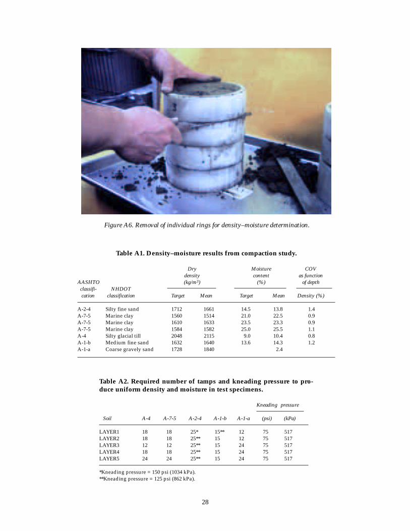
Figure A6. Removal of individual rings for density–moisture determination.

Table A1. Density–moisture results from compaction study.

Dry Moisture COVdensity content as function

AASHTO (kg/m3) (%) of depthclassifi- NHDOTcation classification Target Mean Target Mean Density (%)

A-2-4 Silty fine sand 1712 1661 14.5 13.8 1.4A-7-5 Marine clay 1560 1514 21.0 22.5 0.9A-7-5 Marine clay 1610 1633 23.5 23.3 0.9A-7-5 Marine clay 1584 1582 25.0 25.5 1.1A-4 Silty glacial till 2048 2115 9.0 10.4 0.8A-1-b Medium fine sand 1632 1640 13.6 14.3 1.2A-1-a Coarse gravely sand 1728 1840 2.4

Table A2. Required number of tamps and kneading pressure to pro-duce uniform density and moisture in test specimens.

Kneading pressure

Soil A-4 A-7-5 A-2-4 A-1-b A-1-a (psi) (kPa)

LAYER1 18 18 25* 15** 12 75 517LAYER2 18 18 25** 15 12 75 517LAYER3 12 12 25** 15 24 75 517LAYER4 18 18 25** 15 24 75 517LAYER5 24 24 25** 15 24 75 517

*Kneading pressure = 150 psi (1034 kPa).**Kneading pressure = 125 psi (862 kPa).

28

specimens may be molded at several moisture contents. Therefore, compactionprocedures were developed for three moisture contents. We were unable to splitthe coarse gravelly (A-1-a) material into the individual rings. The material hadvery little fines and there was no cohesion to hold the material in the individualrings. For this material, the density was determined from the total weight of thespecimen. Table A1 shows the target and obtained dry densities, moisture con-tents, and the coefficient of variation of the densities and moisture contents.

To obtain uniform densities, the following number of tamps and kneading pres-sure were used as shown in Table A2. Layer 1 is at the bottom of the mold. Notethat for the A-2-4 and the A-1-b soils, higher kneading pressures on the first layerwere needed 150 and 125 psi (1034 and 862 kPa, respectively). For the remaininglayers of A-2-4, the kneading pressure was decreased to 125 psi (862 kPa), with thesame number of tamps used.

29

30

APPENDIX B: SAMPLE PREPARATION/TESTING

RESILIENT MODULUS TESTING

For resilient modulus test samples, the required amount of test material wassoaked at the required moisture content for 24 hours. The samples were fabricatedusing the procedure in Appendix A.

A membrane is fitted around the bottom cap and securely fastened with two O-rings. The split aluminum mold (Fig. B1) is secured with two hose clamps, and thefasteners should be aligned so that the attaching rods to the bottom plate will passfreely. The membrane is then stretched over the top of the mold and securely fas-tened with an O-ring. For drained tests, a special porous plastic of higher porosityis used. Vacuum is applied through the side of the mold and the membrane is pulledtightly to the sidewalls.

The mold is transferred to the kneading compactor and fastened to the rotatingbase. The first layer of soil is added and tamped with the proper foot (dependingon the diameter of the test specimen). The surface is scarified before the next layeris added. After the last layer has been placed and compacted, it is trimmed care-fully and capped. The cap includes a filter paper and a top cap. The rubber mem-brane is placed over the top cap and then securely fastened with O-rings (Fig. B2).

For the fine-grained soils, the vacuum was released and the specimen trans-ferred to either the MTS machine. For coarse-grained soil, for resilient modulus

Figure B1. Split aluminum mold for specimen prepa-ration.

31

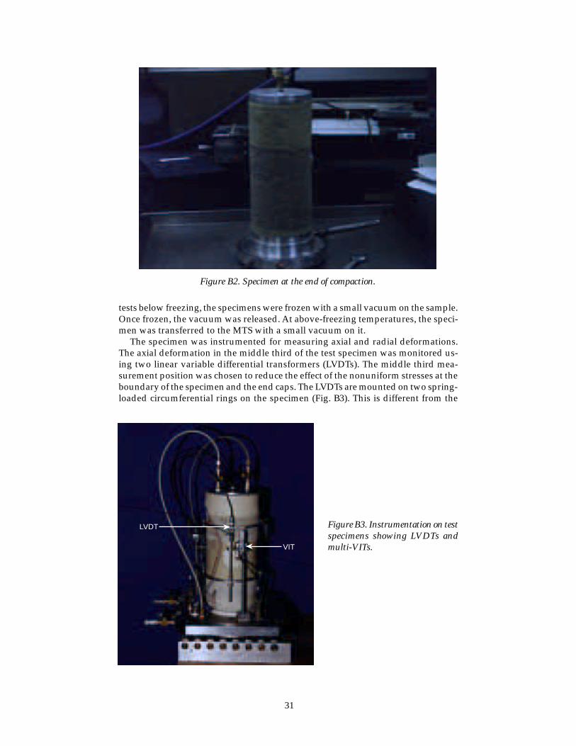
tests below freezing, the specimens were frozen with a small vacuum on the sample.Once frozen, the vacuum was released. At above-freezing temperatures, the speci-men was transferred to the MTS with a small vacuum on it.

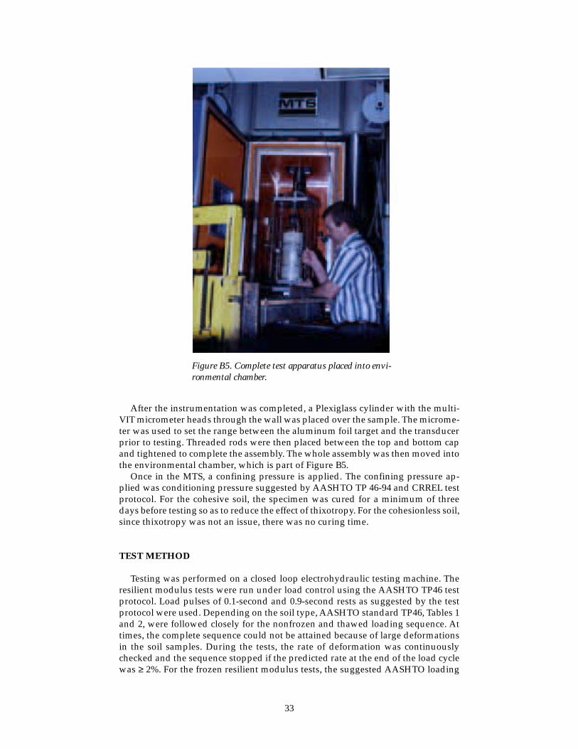
The specimen was instrumented for measuring axial and radial deformations.The axial deformation in the middle third of the test specimen was monitored us-ing two linear variable differential transformers (LVDTs). The middle third mea-surement position was chosen to reduce the effect of the nonuniform stresses at theboundary of the specimen and the end caps. The LVDTs are mounted on two spring-loaded circumferential rings on the specimen (Fig. B3). This is different from the

Figure B2. Specimen at the end of compaction.

Figure B3. Instrumentation on testspecimens showing LVDTs andmulti-VITs.VIT

LVDT ➤

➤

Figure B4. Typical AASHTO triaxial chamber with external LVDTs and load cell.

Specimen

Repeated Load Actuator

Load Cell

Chamber Piston Rod13 mm (0.5 in.) Minimum Diameter for Type 2 Soils38 mm (1.5 in.) Minimum Diameter for Type 1 Soils

LVDT

Cell Pressure Inlet

Cover Plate

Chamber (Lexan or Acrylic)

Tie Rods

Sample Base

Vacuum Inlet Vacuum Inlet

Base Plate

Porous Bronze Diskor Porous Stone

Sample Membrane

Porous Bronze Diskor Porous Stone

O-Ring Seals

Thompson Ball Bushing

LVDT Solid Bracket

51 mm (2 in.) Maximum

Steel BallBall Seat (Divot)

Sample Cap

Solid Base

32

AASHTO TP 46, where the LVDTs are placed on the outside of the chamber (Fig.B4). Deformation of the specimen is inferred from the movement of the loadingpiston rod. Our experience has shown that there can be significant differences be-tween the measurements made from the piston rod and that made on the speci-men. The difference has been attributed to friction as the rod slides through thecover plate. The LVDT barrels are mounted on the top ring and the tips of thespring loaded cores protrude to the bottom ring. An alignment jig was used duringsetup to ensure a uniform gage length for each test. The LVDTs have a range equalto or greater than 5% strain over the gauge length. The 2.8-in.- (71-mm-) diam.,6-in.- (152-mm-) tall specimens have a gauge length of 3 in. (75 mm) and the 6-in.-(152-mm-) diam. and 12-in.- (304-mm-) tall specimens have a gauge length of 6 in.(152 mm).

Radial displacements were measured with three noncontacting displacementtransducers called multipurpose variable impedance transducers (multi-VITs) (Fig.B3). Brass targets were glued on to the specimens around the middle of the speci-men. Each multi-VIT was calibrated with the aluminum foil targets and calibrationcurves of voltage vs. distance obtained. The multi-VITs are mounted on rods thatbolt to the base of the triaxial cell. The position of each transducer is adjusted by amicrometer, which reacts against the spring loaded rod to which the transducer isattached. Early in the research, the three measurements are recorded and averagedfrom which the radial strain and Poisson’s ratio are calculated. Later, we recordedeach signal separately.

33

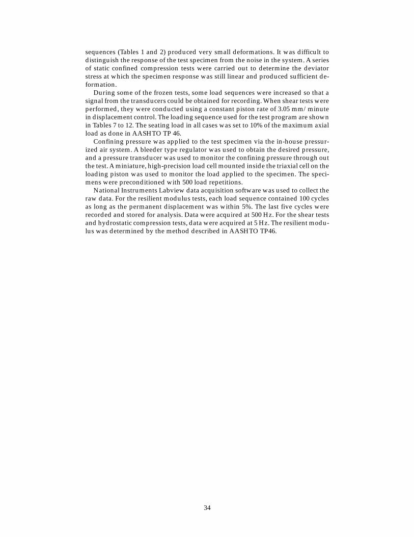
After the instrumentation was completed, a Plexiglass cylinder with the multi-VIT micrometer heads through the wall was placed over the sample. The microme-ter was used to set the range between the aluminum foil target and the transducerprior to testing. Threaded rods were then placed between the top and bottom capand tightened to complete the assembly. The whole assembly was then moved intothe environmental chamber, which is part of Figure B5.

Once in the MTS, a confining pressure is applied. The confining pressure ap-plied was conditioning pressure suggested by AASHTO TP 46-94 and CRREL testprotocol. For the cohesive soil, the specimen was cured for a minimum of threedays before testing so as to reduce the effect of thixotropy. For the cohesionless soil,since thixotropy was not an issue, there was no curing time.

TEST METHOD

Testing was performed on a closed loop electrohydraulic testing machine. Theresilient modulus tests were run under load control using the AASHTO TP46 testprotocol. Load pulses of 0.1-second and 0.9-second rests as suggested by the testprotocol were used. Depending on the soil type, AASHTO standard TP46, Tables 1and 2, were followed closely for the nonfrozen and thawed loading sequence. Attimes, the complete sequence could not be attained because of large deformationsin the soil samples. During the tests, the rate of deformation was continuouslychecked and the sequence stopped if the predicted rate at the end of the load cyclewas ≥ 2%. For the frozen resilient modulus tests, the suggested AASHTO loading

Figure B5. Complete test apparatus placed into envi-ronmental chamber.

34

sequences (Tables 1 and 2) produced very small deformations. It was difficult todistinguish the response of the test specimen from the noise in the system. A seriesof static confined compression tests were carried out to determine the deviatorstress at which the specimen response was still linear and produced sufficient de-formation.

During some of the frozen tests, some load sequences were increased so that asignal from the transducers could be obtained for recording. When shear tests wereperformed, they were conducted using a constant piston rate of 3.05 mm/minutein displacement control. The loading sequence used for the test program are shownin Tables 7 to 12. The seating load in all cases was set to 10% of the maximum axialload as done in AASHTO TP 46.

Confining pressure was applied to the test specimen via the in-house pressur-ized air system. A bleeder type regulator was used to obtain the desired pressure,and a pressure transducer was used to monitor the confining pressure through outthe test. A miniature, high-precision load cell mounted inside the triaxial cell on theloading piston was used to monitor the load applied to the specimen. The speci-mens were preconditioned with 500 load repetitions.

National Instruments Labview data acquisition software was used to collect theraw data. For the resilient modulus tests, each load sequence contained 100 cyclesas long as the permanent displacement was within 5%. The last five cycles wererecorded and stored for analysis. Data were acquired at 500 Hz. For the shear testsand hydrostatic compression tests, data were acquired at 5 Hz. The resilient modu-lus was determined by the method described in AASHTO TP46.

1. AGENCY USE ONLY (Leave blank) 2. REPORT DATE 3. REPORT TYPE AND DATES COVERED

4. TITLE AND SUBTITLE 5. FUNDING NUMBERS

6. AUTHORS

7. PERFORMING ORGANIZATION NAME(S) AND ADDRESS(ES) 8. PERFORMING ORGANIZATION REPORT NUMBER

9. SPONSORING/MONITORING AGENCY NAME(S) AND ADDRESS(ES) 10. SPONSORING/MONITORING AGENCY REPORT NUMBER

11. SUPPLEMENTARY NOTES

12a. DISTRIBUTION/AVAILABILITY STATEMENT 12b. DISTRIBUTION CODE

13. ABSTRACT (Maximum 200 words)

14. SUBJECT TERMS 15. NUMBER OF PAGES

16. PRICE CODE

17. SECURITY CLASSIFICATION 18. SECURITY CLASSIFICATION 19. SECURITY CLASSIFICATION 20. LIMITATION OF ABSTRACT OF REPORT OF THIS PAGE OF ABSTRACT

NSN 7540-01-280-5500 Standard Form 298 (Rev. 2-89)Prescribed by ANSI Std. Z39-18298-102

REPORT DOCUMENTATION PAGEForm ApprovedOMB No. 0704-0188

Public reporting burden for this collection of information is estimated to average 1 hour per response, including the time for reviewing instructions, searching existing data sources, gathering andmaintaining the data needed, and completing and reviewing the collection of information. Send comments regarding this burden estimate or any other aspect of this collection of information,including suggestion for reducing this burden, to Washington Headquarters Services, Directorate for Information Operations and Reports, 1215 Jefferson Davis Highway, Suite 1204, Arlington,VA 22202-4302, and to the Office of Management and Budget, Paperwork Reduction Project (0704-0188), Washington, DC 20503.

September 1999

Resilient Modulus for New Hampshire Subgrade Soils forUse in Mechanistic AASHTO Design

Vincent C. Janoo, Jack J. Bayer Jr., Glenn D. Durell, and Charles E. Smith Jr.

U.S. Army Cold Regions Research and Engineering Laboratory72 Lyme RoadHanover, New Hampshire 03755-1290

Special Report 99-14

Approved for public release; distribution is unlimited.Available from NTIS, Springfield, Virginia 22161

State of New HampshireDepartment of TransportationConcord, New Hampshire 03302

43

UNCLASSIFIED UNCLASSIFIED UNCLASSIFIED UL

Cohesive soils Granular soilsEffective resilient modulus Resilient modulusFreezing Sample preparation

Thawing

Project: 12323P

Resilient modulus tests were conducted on five subgrade soils commonly found in the state of New Hampshire.Tests were conducted on samples prepared at optimum density and moisture content. To determine the effectiveresilient modulus of the various soils for design purposes, tests were conducted at room temperature and at freez-ing temperatures. The AASHTO TP 46 test protocol was used for testing room temperature and thawing soils. Atfreezing temperatures, the CRREL test protocol was used. The results from this test program are presented in thisreport. In addition, suggested effective resilient modulus for the five soils are presented.

Date post:	13-Apr-2018
Category:	Documents
Upload:	truongtruc
View:	220 times
Download:	1 times

Resilient Modulus for New Hampshire Subgrade Soils for … · Resilient Modulus for New Hampshire...

Documents