Retrieval of Land Surface Component Temperature by Particle Swarm Optimization Algorithm
1 Zhenhua LIU, 2 Manqin Hu, 3 Qiaoyi Chen, 4 Yueming Hu ,* WANG Lu 1, 2, *, 4 College of Information, South China Agricultural University, Guangzhou 510642, China
3 Surveying and Mapping Institute Lands and Resource Department of Guangdong Province, Guangzhou 510642, China
* Guangzhou Institute of Geochemistry, Chinese Academic of Science, Guangzhou, 510642, China; * Graduate University of Chinese Academic of Science, Beijing 100039, China;
* Guangdong Province Land Use and Remediation of the Key Laboratory, Guangzhou, 510642, China
Land surface temperature is critical parameter to energy exchange between surface and atmospheric layers. Under the assumption of isothermal surface, current algorithms for retrieving land surface temperature (LST) are mainly general split window, TSE, day-night, directly separate surface temperature from emissivity [1-8]. This surface temperature is
considered as an aggregate over multiple canopy components. However, natural land surfaces are neither homogeneous nor isothermal. The assumption of a single surface temperature is not correct, which cannot meet the practical needs of a quantitative study. And the physical signification of component temperature was distinct, and could improve the quantitative inversion for surface parameters [9, 10]. Directional remote sensing is therefore the best tool
Sensors & Transducers, Vol. 164, Issue 2, February 2014, pp. 256-264
257
for the retrieval of canopy component temperatures. There have recently been many basic theoretical studies on component temperatures, and tried to inverse surface component temperature by considering thermal radiation and emissivity direction characteristics [11-13]. However the information of multi-angular observations is still limited. The objective of this research was to create an inversion scheme to acquire component temperatures in pixels retrieve three component (sunlit soil, shaded soil and vegetable) temperatures. Thus, given spatial resolution of aster reflectance data are higher to structural parameters than TIR data, we developed an inversion strategy to acquire area ratios of components in the pixel, which exploit the information in both VNIR and NIR data.
Given model inversion is still an ill-posed problem, in recent years, based on the thermal radiant formula of open complex system, the components temperature is calculated mainly by optimization methods [14-18]. In this paper, Particle swarm optimization (PSO) is applied to retrieve three component (sunlit soil, shaded soil and vegetable) temperatures. In this work, under no limit condition,
initial particle range in PSO is acquired by histogram in order to reduce the search range and improve the efficiency of the search. And, the ASTER data is used to estimate component temperatures by our model inversion. 2. Materials and Methods 2.1. Study Site and Data
Study area is located in Yingke irrigation area of Heihe River Basin, northwest China (Fig. 1), which is situated in the temperate zone and enjoys a semi-arid climate with hot summers and cold and dry winters. Diurnal temperature ranges tend to be somewhat large due to the high elevation and aridity. The mean annual temperature is 6.5~7.0°C, the maximum temperature of 33.5 °C, while annual rainfall is 125 mm, almost all of which falls from May to October. The winters are so dry that snow is extremely rare. The main types of land cover are wheat, corn and other agricultural land.
(a) TM 321 (b) ASTER 321)
Fig. 1. Yingke working area.
This study uses ASTER from 4 June 2008. Data will be obtained in 14 spectral bands covering the visible through the thermal infrared wavelength region. Five bands of thermal infrared (TIR) data with a noise equivalent temperature difference of 0.3 and three reflectance data is collected to estimate surface temperatures. The three visible bands, which have 15 m resolution, were calibrated by using in situ measurements of spectral reflectance. Five bands in the thermal infrared with 90-m spatial resolution were calibrated by MOTRAN model [19].
Simultaneous Remote Sensing and Ground-based Experiment in the Yingke area are examined to
validate the inversion method and promote the applicability of quantitative remote sensing in component temperature studies. The main crop in the field was wheat and corn, and the field was flat. Wheat rows were oriented east-west at one location and north-south and corn north-south at the other. Canopy (including vegetable, shaded soil and sunlit soil) temperatures were measured with a portable infrared thermometer held at perpendicular to the surface. The observation direction was, the bandwidth of sensor was 8-11 μm and the viewing field angle was 15°.
A
B
Yingke wheat
Yingke corn
Sensors & Transducers, Vol. 164, Issue 2, February 2014, pp. 256-264
258
2.2. Method 2.2.1. Thermal Radiant Model
Because thermal radiant flux of mixed-pixel in studied area is aggregate over soil and vegetable components. In this paper, mixed-pixel is divided into vegetable, shaded soil and sunlit soil. Assuming that the spatial structure of the mixed pixel can be ignored, the surface radiation emitted by the pixel can be written as a weighted linear combination of every component radiation:
)()1()()( 21222111 vbiivSbiisSbiisi TLffTLfTLfL ,
(1) where iL stands for the surface radiance emitted by
the pixel, vT represents vegetation temperature, 1sT
is shaded soil temperature, 2sT stands for sunlit soil
temperature, 1s is the emissivity of the sunlit soil,
2s is the emissivity of the shaded soil, v is the
emissivity of the vegetation, 1f is fractional cover of
the sunlit soil, 2f is fractional cover of the vegetable,
)( 1sbi TL is the broadband blackbody radiation at the
sunlit soil temperature 1sT , )( 2sbi TL is the broadband
blackbody radiation at the sunlit soil temperature 2sT ,
)( vbi TL is the broadband blackbody radiation at the
vegetable temperature vT . The broadband blackbody
radiation is calculated using the Planck blackbody radiation law:
1/
15
22)(
kTche
hcTbL
, (2)
where h is the Planck’s constant (6.626610234 Js), c is the velocity of light (36108 ms21), k is the Boltzmann’s constant (1.38610223 JK21), T is the absolute temperature, and l is the wavelength of the radiation.
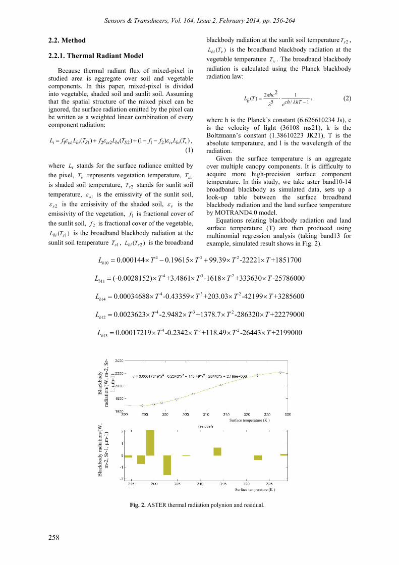
Given the surface temperature is an aggregate over multiple canopy components. It is difficulty to acquire more high-precision surface component temperature. In this study, we take aster band10-14 broadband blackbody as simulated data, sets up a look-up table between the surface broadband blackbody radiation and the land surface temperature by MOTRAND4.0 model.
Equations relating blackbody radiation and land surface temperature (T) are then produced using multinomial regression analysis (taking band13 for example, simulated result shows in Fig. 2).
4 3 2
10 0.000144 0.19615 99.39 -22221 +1851700bL T T T T
4 3 211 (-0.0028152) +3.4861 -1618 +333630 -25786000bL T T T T
4 3 2
14 0.00034688 -0.43359 +203.03 -42199 +3285600bL T T T T
4 3 212 0.0023623 -2.9482 +1378.7 -286320 +22279000bL T T T T
4 3 2
13 0.00017219 -0.2342 +118.49 -26443 +2199000bL T T T T
Bla
ckbo
dy
radi
atio
n/(W
, m-2
, Sr-
1, μ
m-1
)
Surface temperature (K )
Fig. 2. ASTER thermal radiation polynion and residual.
Bla
ckbo
dy r
adia
tion
/(W
, m
-2, S
r-1,
μm
-1)
Surface temperature (K )
Sensors & Transducers, Vol. 164, Issue 2, February 2014, pp. 256-264
259
2.2.2. Retrieving Area Ratios of the Canopy
The thermal radiant model usually contains more parameters than observations. Thus, measurement and model uncertainties make the inverse problem ill posed, inducing difficulties and inaccuracies in the search for the solution. This study focuses on the use of prior information to reduce the uncertainties associated to the estimation of component temperature in the radiative transfer model inversion process. For this purpose, ASTER reflectance data were adapted to account for area ratios of the canopy. Mix-pixel components in the studied area were divided into vegetable, shaded soil and sunlit soil. Canopy fractional cover can be estimated from visible, which canopy is written as:
221211 )1( isviisi ffff , (3)
where i is the spectral reflectance of the surface in
channel i; vi is the spectral reflectance of vegetable
in channel i; 1is is the spectral reflectance of sunlit
soil in channel i; 2is is the spectral reflectance of
shaded soil in channel i. In order to spectral reflectance in channel, atmospheric correction for each visible channel is completed by Modtran model. Linear regression model is applied to resolve area ratios of canopy (Fig. 3).
Fig. 4 gives the values of correlation coefficient R2 which is the measure of the quality of parameter retrieval. As for most pixels, correlations were high for ratios of canopy (R^2 from 0.90 to 1.00), which is shown in Fig. 4.
In canopy area irrigated by water long before, there is low precision (R^2<0.9), which is caused by supersaturated soil moisture. The other irrigated area, the R^2 is relatively high.
Because building reflectance data can not used to acquire ratios of canopy (soil and vegetable), the simulated result is wrong (lager than 1.0) in Sporadic buildings area.
Fig. 3. Area ratios of ASTER Mix-pixel components in the studied area.
2.2.3. Inversion of Component Temperatures Using Particle Swarm Optimization
a). Particle swarm optimization Particle swarm optimization (PSO) is an
algorithm for finding optimal regions of complex
search spaces through the interaction of individuals in a population of particles. In PSO, the particles are placed in the search space of some problem or function, and each evaluates the objective function at its current location. Each particle then determines its movement through the search space by combining
Fig. 4. The correlation coefficients.
a) gray value b) histogram
Pix
el n
umbe
rs /n
a) sunlit soil b) vegetable c) shaded soil
Sensors & Transducers, Vol. 164, Issue 2, February 2014, pp. 256-264
260
some aspect of the history of its own current and best locations with those of one or more members of the swarm, with some random perturbations. The next iteration takes place after all particles have been moved. Eventually the swarm as a whole, like a flock of birds collectively foraging for food, is likely to move close to an optimum of the fitness function. The principle of PSO is shown in Fig. 5.
Where vk is the current velocity; xk is the current position considered as a set of coordinates describing a point in space; vk+1, xk+1 is respectively the next iterative velocity and position; Xpbest is the best solution (fitness) each particle has achieved so far; xgbest is a global best position. The process for implementing PSO is as in Fig. 6.
Fig. 5. The principle of PSO.
Initialize swarm size
Calculate particle Fitness of each particle
Acquiring the best solution of each particle and a global best position
Change the velocity and position
If satisfied condition?
Iteration +1
The global best solution
Yes
No
Fig. 6. PSO algorithm.
Surface component temperature inversion is one of many remote sensing problems which can be identified as a nonlinear multi-parameter optimization problem. Methods based on local linearization fail if the starting model is too far from the true model. Unlike a single simulated annealing run, Particle swarm optimization is a heuristic global optimization technology and also a kind of evolutionary computation technology, which is based on group intelligence. It comes from the research on the bird flock movement behavior. Each particle of the swarm represents one candidate solution of the problem being optimized. The algorithm finds optimal regions of complex problem spaces through the pheromone interaction of particles. Thus, PSO is applied to retrieve component temperature in this study. The objective function of PSO is expressed as:
UR
RXts
Xf
..
min
, (4)
where TnxxxX ,...,, 21 represents a candidate
solution to the optimization problem. R is particles warm. U is the feasible parameter space, f x is
the objective function. In this study on the surface component temperature,
1
n
O Cf x L L
, OL
is the radiance of the ht band, CL is the radiation
computed using equation (3) for the th . Each particle in the swarm represents a candidate solution to the optimization problem. Thus, the candidate
solution for the equation
n
CO LLxf1
is
expressed as x=( soil , soilT , v , vT , shadesoil , shadesoilT ).
b). PSO parameters setting PSO represents an efficient search method for
nonlinear optimization problems. In a comparative analysis of general differential equation, the initial parameter ranges are set more available. A particle decides where to move next, considering its own experience, which is the memory of its best past position, and the experience of its most successful particle in the swarm. In the particle swarm model, the particle searches the solutions in the problem space with a given range. In order to guide the particles effectively in the search space, the maximum moving distance during one iteration must be clamped in between the maximum velocity. Most researchers use a swarm size of 10 to 50 but there is no well established guideline [20], the swarm size is fixed at 40 particles in the PSO swarm. Particle sizes
of the particles ( soil , soilT , v , vT , shadesoil , shadesoilT )
are six. In this study, to reduce the search range and improve the efficiency of the search, the ranges of particle are acquired by histogram method [21]. PSO initial particle were given the following ranges: [287, 323], [273, 303], [273, 333],
Sensors & Transducers, Vol. 164, Issue 2, February 2014, pp. 256-264
261
[0.85, 0.92], [0.8, 1.00], [0.5, 1.00]. And, the last parameter search range for vegetable is set to [0.95, 1.00], [280, 310].
1) Determining the optimal combination of PSO parameters
The Convergence properties and speed of the PSO depends mainly on some parameters including c1, c2, and w and so on. c1 is a positive constant, called as coefficient of the self-recognition component; c2 is a positive constant, called as coefficient of the social component.
The variable w is called as the inertia factor, which value is typically setup to vary linearly from 1 to near 0 during the iterated processing. In fact, without distinct physical-mathematical bases, the best parameters are acquired by randomized trial. In this paper, the Yingke wheat studied area (A) is selected. The field measured wheat temperature is 26.2°С, sunlit soil temperature is 41.7°С, shaded soil temperature is 22.1°С. Particle scopes were given the following ranges: [0.85, 0.92], [0.8, 1.00], [0.95, 1.00], [287, 323], [273, 303], [280, 310]. The maximum generation (iterations) is set as 300. The swarm size is fixed at 40. The particle position is updated using its current value and newly computed velocity affected by coefficients which is set as 0.0048 in tests.
The simulated result is shown in Table 1. The research presented in this paper found out that setting the three weight factors w, c1, and c2 at 0.98, 0.5, and 0.2 respectively provides the best convergence rate for the tests.
2) Determining the maximum generation The experiment was still centered on wheat
site (A). The set parameters are follow as: the swarm size is fixed at 40; the coefficients affected particle
current value and newly computed velocity is set as 0.0048; The initial Particle scopes were given the following ranges: [0.85, 0.95], [0.85, 0.95], [0.85, 0.95], [273, 323], [273, 303], [273, 308]. The simulated component temperature is shown in Fig. 7 with maximum generation changes between 25 to 300.
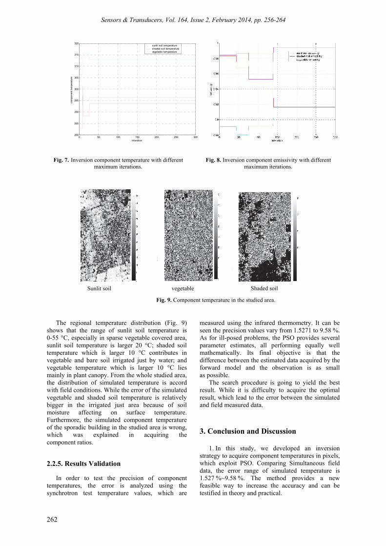
The above result reveals that the curves of simulated component temperatures and emissivity fluctuate more frequent when the maximum generation is between 0 and 150. While the maximum generation is 200, the simulated temperatures are near to filed measured data. Thus, in this study, the maximum generation is set as 300.
2.2.4. Component Temperatures Inversion
According to equation (1), component
temperature parameters including the sunlit soil temperature, the shaded soil temperature, the vegetation temperature, the emissivity of the soil and vegetable in the five bands are retrieved. Because the number of inversed parameters is greater than independent equations, it is an underdetermined problem. In order to improve inversed precision, the area ratios of components were used from VNIR and NIR data.
PSO initial parameters were given the following ranges: [0.85, 0.95], [0.85, 0.95], [0.85, 0.95], [273, 323], [273, 303], [273, 308]. The maximum generation is 300. The retrieved component temperatures are shown in Fig. 8 and Fig. 9.
Table 1. Inversion results (m=40 population size 564, maximum iterations=300).
w
0.7 0.85 0.98
a=0.0048
c1
0.8
T 25.77 29.13 40.70 21.50 29.01 15.76 29.25 28.67 27.33
Sensors & Transducers, Vol. 164, Issue 2, February 2014, pp. 256-264
262
Fig. 7. Inversion component temperature with different maximum iterations.
Fig. 8. Inversion component emissivity with different maximum iterations.
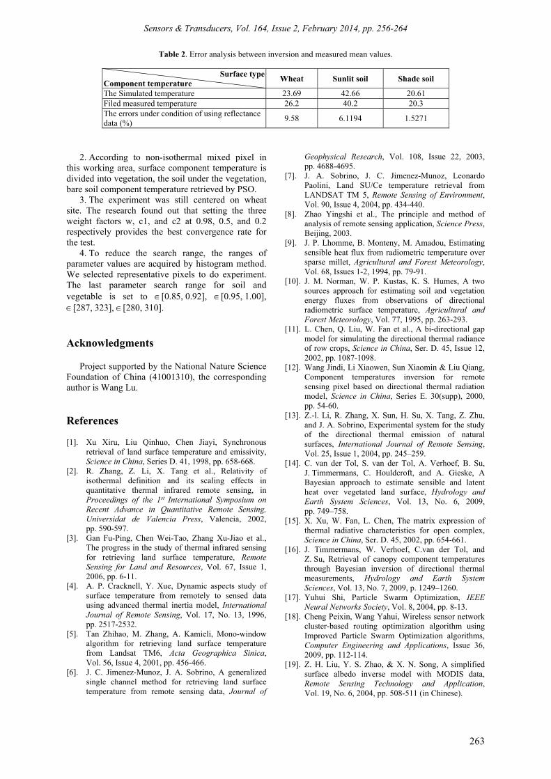
Fig. 9. Component temperature in the studied area.
The regional temperature distribution (Fig. 9)
shows that the range of sunlit soil temperature is 0-55 °C, especially in sparse vegetable covered area, sunlit soil temperature is larger 20 °C; shaded soil temperature which is larger 10 °C contributes in vegetable and bare soil irrigated just by water; and vegetable temperature which is larger 10 °C lies mainly in plant canopy. From the whole studied area, the distribution of simulated temperature is accord with field conditions. While the error of the simulated vegetable and shaded soil temperature is relatively bigger in the irrigated just area because of soil moisture affecting on surface temperature. Furthermore, the simulated component temperature of the sporadic building in the studied area is wrong, which was explained in acquiring the component ratios.
2.2.5. Results Validation
In order to test the precision of component temperatures, the error is analyzed using the synchrotron test temperature values, which are
measured using the infrared thermometry. It can be seen the precision values vary from 1.5271 to 9.58 %. As for ill-posed problems, the PSO provides several parameter estimates, all performing equally well mathematically. Its final objective is that the difference between the estimated data acquired by the forward model and the observation is as small as possible.
The search procedure is going to yield the best result. While it is difficulty to acquire the optimal result, which lead to the error between the simulated and field measured data.
3. Conclusion and Discussion
1. In this study, we developed an inversion strategy to acquire component temperatures in pixels, which exploit PSO. Comparing Simultaneous field data, the error range of simulated temperature is 1.527 %~9.58 %. The method provides a new feasible way to increase the accuracy and can be testified in theory and practical.
0 50 100 150 200 250 300280
285
290
295
300
305
310
315
320
interation
com
pone
nt t
empe
ratu
re
sunlit soil temperature shaded soil temperaturevegetable temperature
Sunlit soil vegetable Shaded soil
Sensors & Transducers, Vol. 164, Issue 2, February 2014, pp. 256-264
263
Table 2. Error analysis between inversion and measured mean values.
Surface typeComponent temperature Wheat Sunlit soil Shade soil
The Simulated temperature 23.69 42.66 20.61 Filed measured temperature 26.2 40.2 20.3 The errors under condition of using reflectance data (%) 9.58 6.1194 1.5271
2. According to non-isothermal mixed pixel in this working area, surface component temperature is divided into vegetation, the soil under the vegetation, bare soil component temperature retrieved by PSO.
3. The experiment was still centered on wheat site. The research found out that setting the three weight factors w, c1, and c2 at 0.98, 0.5, and 0.2 respectively provides the best convergence rate for the test.
4. To reduce the search range, the ranges of parameter values are acquired by histogram method. We selected representative pixels to do experiment. The last parameter search range for soil and vegetable is set to [0.85, 0.92], [0.95, 1.00], [287, 323], [280, 310]. Acknowledgments
Project supported by the National Nature Science Foundation of China (41001310), the corresponding author is Wang Lu.
References [1]. Xu Xiru, Liu Qinhuo, Chen Jiayi, Synchronous
retrieval of land surface temperature and emissivity, Science in China, Series D. 41, 1998, pp. 658-668.
[2]. R. Zhang, Z. Li, X. Tang et al., Relativity of isothermal definition and its scaling effects in quantitative thermal infrared remote sensing, in Proceedings of the 1st International Symposium on Recent Advance in Quantitative Remote Sensing, Universidat de Valencia Press, Valencia, 2002, pp. 590-597.
[3]. Gan Fu-Ping, Chen Wei-Tao, Zhang Xu-Jiao et al., The progress in the study of thermal infrared sensing for retrieving land surface temperature, Remote Sensing for Land and Resources, Vol. 67, Issue 1, 2006, pp. 6-11.
[4]. A. P. Cracknell, Y. Xue, Dynamic aspects study of surface temperature from remotely to sensed data using advanced thermal inertia model, International Journal of Remote Sensing, Vol. 17, No. 13, 1996, pp. 2517-2532.
[5]. Tan Zhihao, M. Zhang, A. Kamieli, Mono-window algorithm for retrieving land surface temperature from Landsat TM6, Acta Geographica Sinica, Vol. 56, Issue 4, 2001, pp. 456-466.
[6]. J. C. Jimenez-Munoz, J. A. Sobrino, A generalized single channel method for retrieving land surface temperature from remote sensing data, Journal of
Geophysical Research, Vol. 108, Issue 22, 2003, pp. 4688-4695.
[7]. J. A. Sobrino, J. C. Jimenez-Munoz, Leonardo Paolini, Land SU/Ce temperature retrieval from LANDSAT TM 5, Remote Sensing of Environment, Vol. 90, Issue 4, 2004, pp. 434-440.
[8]. Zhao Yingshi et al., The principle and method of analysis of remote sensing application, Science Press, Beijing, 2003.
[9]. J. P. Lhomme, B. Monteny, M. Amadou, Estimating sensible heat flux from radiometric temperature over sparse millet, Agricultural and Forest Meteorology, Vol. 68, Issues 1-2, 1994, pp. 79-91.
[10]. J. M. Norman, W. P. Kustas, K. S. Humes, A two sources approach for estimating soil and vegetation energy fluxes from observations of directional radiometric surface temperature, Agricultural and Forest Meteorology, Vol. 77, 1995, pp. 263-293.
[11]. L. Chen, Q. Liu, W. Fan et al., A bi-directional gap model for simulating the directional thermal radiance of row crops, Science in China, Ser. D. 45, Issue 12, 2002, pp. 1087-1098.
[12]. Wang Jindi, Li Xiaowen, Sun Xiaomin & Liu Qiang, Component temperatures inversion for remote sensing pixel based on directional thermal radiation model, Science in China, Series E. 30(supp), 2000, pp. 54-60.
[13]. Z.-l. Li, R. Zhang, X. Sun, H. Su, X. Tang, Z. Zhu, and J. A. Sobrino, Experimental system for the study of the directional thermal emission of natural surfaces, International Journal of Remote Sensing, Vol. 25, Issue 1, 2004, pp. 245–259.
[14]. C. van der Tol, S. van der Tol, A. Verhoef, B. Su, J. Timmermans, C. Houldcroft, and A. Gieske, A Bayesian approach to estimate sensible and latent heat over vegetated land surface, Hydrology and Earth System Sciences, Vol. 13, No. 6, 2009, pp. 749–758.
[15]. X. Xu, W. Fan, L. Chen, The matrix expression of thermal radiative characteristics for open complex, Science in China, Ser. D. 45, 2002, pp. 654-661.
[16]. J. Timmermans, W. Verhoef, C.van der Tol, and Z. Su, Retrieval of canopy component temperatures through Bayesian inversion of directional thermal measurements, Hydrology and Earth System Sciences, Vol. 13, No. 7, 2009, p. 1249–1260.
[18]. Cheng Peixin, Wang Yahui, Wireless sensor network cluster-based routing optimization algorithm using Improved Particle Swarm Optimization algorithms, Computer Engineering and Applications, Issue 36, 2009, pp. 112-114.
[19]. Z. H. Liu, Y. S. Zhao, & X. N. Song, A simplified surface albedo inverse model with MODIS data, Remote Sensing Technology and Application, Vol. 19, No. 6, 2004, pp. 508-511 (in Chinese).
Sensors & Transducers, Vol. 164, Issue 2, February 2014, pp. 256-264
264
[20]. Parag Puranik, Preeti Bajaj, Ajith Abraham, Prasanna Palsodkar, and Amol Deshmukh, Human perception-based color image segmentation using comprehensive learning particle swarm optimiazation, Journal of Information Hiding and Multimedia Signal Processing, Vol. 2, No. 3, 2011, pp. 227-235.
[21] Z. Liu, and Y. Zhao, Retrieval of plant and soil component temperature under different light conditions based on genetic algorithm, Transactions of the Chinese Society of Agricultural Engineering, Vol. 28, No. 1, 2012, pp. 161-166 (in Chinese).