Revisiting ASEAN enlargement effects on trade: A gravity

approach

NGUYEN Thi Nguyet Anh*◊1 , PHAM Thi Hong Hanh*, VALLÉE Thomas*

Preliminary version

*LEMNA, Institute of Economics and Management, University of Nantes, France

◊ Faculty of Business Management, National Economics University, Hanoi, Vietnam

Abstract

The present paper employs the augmented gravity model to examine the impacts of FTAs

between ASEAN and China, Japan and Republic of Korea on the intra-regional export

market. Together with traditional variables, we also introduce in our gravity the network

indicators and take into account the potential endogeneity. Our empirical estimation is

based on a data sample covering both aggregated and disaggregated intra-ASEAN+3

exports over the period 1990 - 2015. This study reveals a set of important findings. First,

we find evidence that the joining of China, South Korea has the positive effects on

fostering intra-ASEAN+3 bilateral trade flows. However, the impacts of the ASEAN -

Japan FTA is not revealed in many cases. Second, by using the commodity data classified

by SITC Revision 3 at one digit level, our empirical results show that the impacts of

ASEAN +1 FTAs on intra-regional trade vary among industrial sectors. Finally, our

results also suggest that with an important position in ASEAN+3’s trade network, a

country member can positively influence ASEAN+3’s bilateral trade among ASEAN+3.

JEL: F02; F10; F14; F40.

Keywords: gravity model; trade network; FTA; ASEAN+3

1 Corresponding author: Thi Nguyet Anh Nguyen; LEMNA-IEMN-IAE, Chemin de la Censive du Tertre, BP 52231, 44322 Nantes Cedex 3, France. Tel: +33 750 992379; Fax: +33 (0)2 40 14 16 50; Email address: thi-nguyet-anh.nguyen1@univ-nantes.fr

1. Introduction

Since 1997, ASEAN Plus Three (ASEAN+3) cooperation has broadened and deepened.

Covering ten ASEAN member states and three East Asian countries (China, Japan and

Korea or Plus Three), ASEAN+3 has been considered as the most successful model of

economic cooperation in Asia (i.e. Kawai and Wignaraja, 2007; Verico, 2013; Kusnadi and

Sitorus, 2014). Despites challenges derived from uncertainties in the global economy,

ASEAN’s trade with Plus Three countries has retained its momentum. In 2015, ASEAN

total trade with the Plus Three countries recorded an increase of 1.7 percent year-on-year,

achieving USD 706.3 billion and accounting for 32.1 percent of ASEAN’s total trade.

In terms of exports, as displayed in Figure (1), the exports from ASEAN to the Plus Three

have increased dramatically since 2002 and only had downward trend in 2007 and 2008

due to the impact of global crisis. Apparently, there has been a big change in the trade

relation between ASEAN and China, especially since 2005. Indeed, the signing FTA

between China and ASEAN (ACFTA) in 2002 and in effect in 2005, which focused on

reducing bilateral tariffs especially on agricultural goods, has promoted trade among

ASEAN members and China. According to the statistics of UNCOMTRADE, this event

has changed the export share of ASEAN to China from 1.82 percent to 13.38 percent over

two decades, and the total trade increased more than tenfold between 2000 and 2015 from

about USD 33 billion to USD 403 billion. As accordance, the tariffs of merchandise goods

are aimed to cut to zero by 2010 for ASEAN -6 (Thailand, Malaysia, Singapore, Indonesia,

Philippines and Brunei), by 2016 for Vietnam and by 2018 for Cambodia, Laos and

Myanmar. Besides the ACFTA, the ASEAN also officially investigated in the FTAs with

South Korea (2007) and Japan (2008), hereafter AKFTA (ASEAN - Republic of Korea FTA)

and AJCEP (ASEAN-Japan Comprehensive Economic Partnership), respectively. The

exports between ASEAN and these two countries have increased over observation

period; nevertheless, the share of exports from ASEAN to Japan in the ASEAN's total

exports has declined about 18.9 percent in 1990 to 8.42 percent in 2015 as presented in

Table (1) to condescend for China.

Figure 1: Exports between ASEAN and Plus Three, 1990 – 2015

Regarding the trade issues of ASEAN and East Asia, several empirical studies have been

developed by using different models and techniques. For instance, Yang and Vines (2000)

use the Global Trade Analysis Project (GTAP) model with differentiated products to

examine the impact of China’s growth over the period 1975-1995. They find that the

increased exports to China leads to the negative effects on new industrializing economies

(NIEs) terms of trade as a result of increased competition in third market. Basing on

Computable General Equilibrium (CGE) model, Chirathivat (2002) provides a sectoral

analysis to address the impacts of ACFTA (ASEAN-China Free Trade Agreement). The

author concludes that the ACFTA would lead to an increase in GDP growth in both China

and ASEAN. Differently, Li and Song (2005), by using export similarity indices computed

at decomposition commodity level to analyze the specialization in ASEAN + 3 trade

integration, point out the convergence in the export structures between China and

Malaysia, Thailand and Singapore with the stable similarities over the period 1995–2003.

Most recently, Nguyen et al. (2016) developed a network analysis to examine the level of

trade integration in ASEAN+3 and to define the role of each country in the bloc. The

authors indicate that large and/or advanced countries seem to be better linked and form

a sub-regional bloc of tightly connected economies only in terms of export absolute value.

Together with the above listed studies, ASEAN and East Asia’s trade issues have been

also widely analyzed in the gravity model framework, which is first pioneered by

Tinbergen (1962), for example: the determinant factors of ASEAN FTA (Hapsari and

Mangunsong, 2006); China’s trade displacement effects (Eichengreen et al., 2004); trade

creation and diversion effects of ASEAN – China FTA (Yang and Martinez-Zarzoso,

2014), and so on.

Table 1: Export share of ASEAN members to Plus Three

ASEAN Member

1990 2000

Intra-ASEAN China Japan Korea EU

Intra-ASEAN China Japan Korea EU

ASEAN 18.95 1.82 18.90 3.34 10.94 22.97 3.84 13.44 3.68 11.30

Brunei 20.93 0.14 58.09 12.37 0.11 23.16 1.76 40.67 12.87 0.28

Cambodia 74.56 0.39 7.58 0.00 4.41 5.58 1.74 0.79 0.06 10.21

Indonesia 9.96 3.25 42.52 5.31 8.91 17.52 4.46 23.21 6.95 11.25

Malaysia 29.45 2.10 15.32 4.62 9.70 26.56 3.09 13.02 3.30 10.17

Philippines 7.27 0.75 19.79 2.80 12.94 15.65 1.74 14.68 3.07 13.72

Singapore 22.35 1.51 8.75 2.22 10.74 27.37 3.90 7.54 3.56 11.03

Thailand 11.93 1.17 17.21 1.71 16.17 19.34 4.07 14.73 1.83 11.69

Vietnam 13.81 0.31 13.48 1.06 6.67 18.09 10.61 17.78 2.44 15.65

ASEAN Member

2010 2015

Intra-ASEAN China Japan Korea EU

Intra-ASEAN China Japan Korea EU

ASEAN 25.06 10.86 9.85 4.30 8.50 23.85 13.38 8.42 3.88 8.23

Brunei 10.53 7.04 0.04 16.75 45.20 18.41 1.48 35.61 14.73 0.38

Cambodia 12.58 1.16 11.89 0.44 1.60 12.65 5.09 7.40 1.65 24.03

Indonesia 21.13 9.94 9.15 7.97 16.34 22.32 10.12 11.85 5.07 8.01

Malaysia 25.38 12.54 8.86 3.80 10.46 25.28 15.95 8.41 3.14 7.05

Philippines 22.47 11.09 12.87 4.33 15.22 13.73 15.14 18.25 4.34 9.49

Singapore 30.26 10.36 7.45 4.09 4.66 29.83 13.73 4.35 4.13 6.82

Thailand 22.92 11.11 7.44 1.87 10.51 25.72 11.07 9.37 1.91 7.08

Vietnam 14.82 10.47 12.48 4.43 11.07 11.73 13.27 8.44 5.47 13.67

Over the last decade, ASEAN +1 FTAs were signed and have been into force; however,

the possible effects of FTA establishment between ASEAN and Plus Three countries on

trade integration and regional economy has been an under-developed issue in the

literature. Therefore, the objective of this paper is to evaluate the effects of ASEAN -

China FTA on intra-regional trade integration, which will be also compared with those

of ASEAN – Japan and ASEAN – Korea FTA by applying an augmented gravity model.

Moreover, to the best of our knowledge, there has been few researches using network

indicators in a gravity model to explain the trade relations. Therefore, a set of trade

network indicators will be added in our gravity model to investigate the role of each

country member in ASEAN+3’s trade network.

To complete the existing literature, the present paper employs the augmented gravity

model to examine the impacts of FTAs between ASEAN and China, Japan and Republic

of Korea (or South Korea) on the intra-regional export market. Together with traditional

variables, we also introduce in our gravity the network indicator and take into account

the potential endogeneity. Our empirical estimation is based on a data sample covering

both aggregated and disaggregated intra-ASEAN+3 exports over the period 1990 - 2015.

This study reveals a set of important findings. First, we found evidence that ASEAN -

China FTA (ACFTA) and ASEAN - Korea FTA (AKFTA) have the positive effects on

fostering intra-ASEAN+3 bilateral trade flows. However, the impact of ASEAN-Japan

FTA (AJFTA) revealed to have reversed effect. Second, by using the commodity data

classified by SITC Revision 3 at one digit level, our empirical results show that the

impacts of ASEAN +1 FTAs on intra-regional trade vary among different sectors. Finally,

our results also suggest that with an important position in ASEAN+3’s trade network, a

country member can positively influence ASEAN+3’s bilateral trade among ASEAN+3.

The remainder of the paper is organized as follows. Section 2 provides a literature about

the impacts of FTAs on bilateral trade with gravity approach. Section 3 presents the

empirical methodology and describes the panel dataset. All the estimation methods and

result discussion are reported in Section 4. Finally, concluding remarks are in Section 5.

2. FTA's impacts to trade: A gravity approach

Our analysis is based on gravity model, which was early pioneered by Timbergen (1962).

Initially, the gravity equation was merely a presentation of an empirically relationship

between the size of economies, their geographical distance and the volume of their trade.

Based on this idea, Anderson (1979) provided a theoretical basis for gravity equation built

on a constant elasticity of substitution (CES), which has become a widely accepted in

subsequent works. In particular, Bergstrand (1985 and 1989) unveiled that the gravity

model is a model of trade based on monopolistic competition developed by Krugman

(1980). While Eaton and Kortum (2002) built the gravity model from a Ricardian type of

model, Helpman et al.(2008) derived it from a theoretical model off international trade in

differentiated goods with firm heterogeneity. In addition, we also pay attention to the

widely cited model developed by Anderson and Van Wincoop (2003), which pointed out

that the cost of bilateral trade are not only affected by geographical factors, but also by

the relative weight of these trade costs in comparison to trading partners in the rest of the

world, namely multilateral resistance terms. As a commonly used framework, the gravity

model has been applied extensively in empirical studies over more than four decades.

Among them, the analysis of regional trade agreements effects by introducing dummy

variables is the key issue.

Frankel et al.(1995) examined the effects of the EU (European Union), the NAFTA (North

American Free Trade Agreement), the MERCOSUR2and the AFTA (ASEAN Free Trade

Agreement), and they found significant positive effects of the MERCOSUR and the AFTA

to trade flows, but not in the cases of the EU and the NAFTA. The trade creation and

trade diversion from the establishment of EEC (European Economic Community),

LAFTA (Latin American Free Trade Association) and CMEA (Council of Mutual

Economic Assistance) are introduced by Endoh (1999). Following the author's findings,

there is no strong evidence that the EEC and the LAFTA trade with Japan any more or

less than the hypothetical level predicted by basic explanatory variables, while the CMEA

increased its trade with Japan up to the hypothetical level during the analysis period. In

recent years, Baier and Bergstrand (2002) tackled the endogeneity issues by treating FTA

dummies as endogenous variables, and they found that the effect of FTAs on trade flow

is quadrupled. Five years later, these authors also used country - pair fixed effects in

addition to time-varying in order to obtain unbiased estimates caused by endogeneity

2 An economic and political bloc comprising Argentina, Brazil, Paraguay, Uruguay and Venezuela, which was suspended on December 1, 2016.

(Baier and Bergstrand, 2007). This method is applied by Carrere (2003) with the panel

data, and the result shows that FTAs generated a significant increase in trade.

Together with the studies of FTAs in world trade, ASEAN and East Asia’s trade issues

have been also widely analyzed in the gravity model framework. Filippini and Molini

(2003) attempted to use the modified gravity model to study trade flows between East

Asian industrializing countries (including China) with the regional dummies. They

found that newly industrializing Asian countries might be considered among the leading

actors of the rapid trade expansion between advanced and developing countries. Based

on the two-way error component form of the gravity model, Nguyen and Hashimoto

(2005) employed Hausman - Taylor estimation to explore the determinants of trade flows

of Asean Free Trade Area (AFTA). Accordingly, the study shows that the AFTA has only

generated the trade creation among its members. However, in the study of Clarete et al.

(2003), by estimation of PTAs impacts to trade in Asia-Pacific, the authors found that the

trade creation of AFTA is seemed to be effective with the founding members, while the

new AFTA members are less integrated with the world economy. By including two

indexes, namely "`complimentary index"' and "`similarity index"' as the determinant

factors of ASEAN FTA, Hapsari and Mangunsong (2006) confirmed that the more

complementary the supply and demand of countries, the more they will trade. Moreover,

similar structure of export between ASEAN members has a positive effect on its bilateral

exports. Estrada et al. (2011) compared the impact of ASEAN+ China, Japan, and Korea

FTA (hereafter ASEAN+3 FTA) and existing ASEAN+1 FTAs on the economic welfare of

member countries by using the Global Trade Analysis Project (GTAP) model. They found

that ASEAN+3 FTA has the advantage of feasibility and desirability for ASEAN members

and China, Japan, and Korea.

With the perception that the impact of FTAs on trade differs depending on the products,

several studies have been conducted at disaggregated sector levels. Notably, Gilbert,

Scollay and Bora (2004) applied both gravity model and CGE (Computable General

Equilibrium) approaches to find out the effects of major FTAs and natural trading blocs

in East Asia by sector. Most recently, the trade integration across manufacturing

industries in EU is explored by Chen and Novy (2011), which is measured by

incorporating substitution elasticities estimated at industry level with gravity model. The

authors found that the significant impact of technical barrier to trade in certain industries.

Yang and M.Zarzoso (2014) justified gravity model to examine the impact of the ASEAN

- China Free Trade Agreement (ACFTA) on exports by using multilateral resistance terms.

The authors confirmed that ACFTA has significant positive impacts in both agricultural

and manufactured goods.

In the shed-light of earlier studies about the effects of FTAs to trade flows, in this paper

we extend our analysis by creating new variables, namely trade network indicators, with

the aim to examine the effect of country's role in ASEAN+3 trade network to bilateral

trade. Moreover, further to our knowledge, there has not been typical studies about the

simultaneous effects of single FTAs between ASEAN and China, Japan and South Korea

to bilateral trade in the ASEAN+3 trading bloc. Therefore, we would like to investigate

into these relation by using an up-to-date data sample comprising aggregated and

disaggregated data set in order to deepen our understanding of the impacts of FTAs in

ASEAN+3.

3. Empirical methodology and Data 3.1. Gravity model

We conduct the estimation of gravity model to assess the impacts of FTAs between

ASEAN and individual "Plus Three" country (China, Japan and South Korea) on bilateral

exports. Moreover, we also develop this empirical work by applying the augmented

gravity equation to test the possible effects of the country's role in ASEAN+3's trade

network on trade flows. With respect to the standard gravity equation, we estimate the

following equation to examine ASEAN+1 FTAs’ effects and network indicator for exports

between exporters and importers:

ln(Xijt) = 𝛼1 + 𝛽11ln𝑌𝑖𝑡 + 𝛽12ln𝑌𝑗𝑡 + 𝛽13𝑁𝑊𝑖(𝑡−1) + 𝛽14𝐴𝐶𝐹𝑇𝐴𝑖𝑗 + 𝛽15𝐴𝐽𝐹𝑇𝐴𝑖𝑗

+ 𝛽16𝐴𝐾𝐹𝑇𝐴𝑖𝑗 + 𝛾11ln𝐸𝑑𝑢𝑐𝑖𝑡 + 𝛾12ln𝐶𝑃𝐼𝑖𝑡 + 𝛾13ln𝑇𝑖𝑗𝑡 + 𝛾14ln𝑅𝐸𝑅𝑖𝑗𝑡

+ 𝛾15ln𝑃𝑂𝑃𝑖𝑡 + 𝛾16ln𝑃𝑂𝑃𝑗𝑡 + 𝜑11ln𝐷𝑖𝑠𝑡𝑖𝑗 + 𝜑12𝐵𝑜𝑟𝑖𝑗 + 𝜑13𝐿𝑎𝑛𝑔𝑖𝑗

+ 𝜑14𝐶𝑜𝑚𝑐𝑜𝑙𝑖𝑗 + ɛ1𝑖𝑗𝑡

(1)

In addition, bilateral exports are also affected by the exporter's educational level of

workers Educit and price level CP Iit which reflected by consumer price index following

Baier and Bergdtrand (2001). The model also include the bilateral average tariff Tijt, ,real

bilateral exchange rate RERijt 3 and several indicators of trade costs: Distij indicates the

geographical distance in km between the largest cities of countries i and j; Borij, Langij

and Comcolij is given the value of unity if countries i and j share the common border,

common official language and same colony. Finally the unobservable terms are absorbed

into the error term ɛ1𝑖𝑗𝑡.

Among the regressors, Y is proxy for income level and is expected to have positive sign

in estimation because the higher income level promotes trade. In terms of network

indicators (𝑁𝑊𝑖(𝑡−1)), the out-degree centrality to measure the connection of the exporter

3 The bilateral real exchange rate is calculated as the product of nominal exchange rate and relative GDP deflator in each country: RERij= 𝑒𝑖𝑗𝑡*(𝑝𝑗𝑡/𝑝𝑖𝑡), where 𝑒𝑖𝑗𝑡 is nominal

exchange rate (IMF, International Financial Statistics), (𝑝𝑗𝑡 is GDP deflator of exporter,

𝑝𝑖𝑡 is GDP deflator of importer.

to other countries in the ASEAN + 3's trade network, which takes into consideration the

direct links of a node and its nearest neighborhood, but ignore the position of a node in

the network’s structure (Nguyen et al., 2016). The eigenvector centrality index, which is

initialed by Bonacich (1972), measures the importance of a node in terms of its connection

to other central nodes (Iapadre and Tajoli, 2014). The coefficients of these two variables

are expected to be positive signs. In this paper, we only use the eigenvector to avoid

autocorrelation. The distance variable reflects both tangible and intangible trade costs

which is expected to have negative sign as the longer the distance, the larger the cost.

The variables of common border, language and colony also reflect trade costs and cultural

similarity, so that these estimated coefficients are expected to be positive. The binary

variable FTAs are expected to be positive with trade creation effect and negative with

trade diversion effect. Our main interest are the signs of the coefficients of the exporter's

network indicator β13 and the free trade agreements β14, β15 and β16.

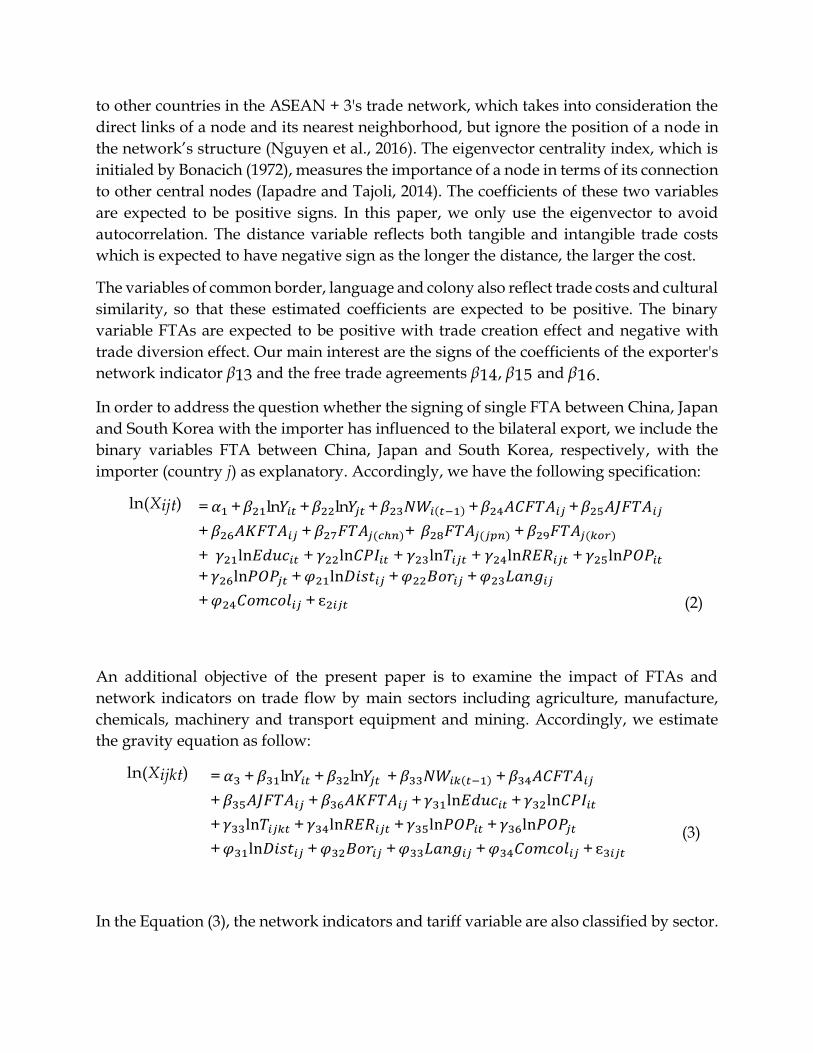
In order to address the question whether the signing of single FTA between China, Japan

and South Korea with the importer has influenced to the bilateral export, we include the

binary variables FTA between China, Japan and South Korea, respectively, with the

importer (country j) as explanatory. Accordingly, we have the following specification:

ln(Xijt) = 𝛼1 + 𝛽21ln𝑌𝑖𝑡 + 𝛽22ln𝑌𝑗𝑡 + 𝛽23𝑁𝑊𝑖(𝑡−1) + 𝛽24𝐴𝐶𝐹𝑇𝐴𝑖𝑗 + 𝛽25𝐴𝐽𝐹𝑇𝐴𝑖𝑗

+ 𝛽26𝐴𝐾𝐹𝑇𝐴𝑖𝑗 + 𝛽27𝐹𝑇𝐴𝑗(𝑐ℎ𝑛)+ 𝛽28𝐹𝑇𝐴𝑗(𝑗𝑝𝑛) + 𝛽29𝐹𝑇𝐴𝑗(𝑘𝑜𝑟)

+ 𝛾21ln𝐸𝑑𝑢𝑐𝑖𝑡 + 𝛾22ln𝐶𝑃𝐼𝑖𝑡 + 𝛾23ln𝑇𝑖𝑗𝑡 + 𝛾24ln𝑅𝐸𝑅𝑖𝑗𝑡 + 𝛾25ln𝑃𝑂𝑃𝑖𝑡

+ 𝛾26ln𝑃𝑂𝑃𝑗𝑡 + 𝜑21ln𝐷𝑖𝑠𝑡𝑖𝑗 + 𝜑22𝐵𝑜𝑟𝑖𝑗 + 𝜑23𝐿𝑎𝑛𝑔𝑖𝑗

+ 𝜑24𝐶𝑜𝑚𝑐𝑜𝑙𝑖𝑗 + ɛ2𝑖𝑗𝑡

(2)

An additional objective of the present paper is to examine the impact of FTAs and

network indicators on trade flow by main sectors including agriculture, manufacture,

chemicals, machinery and transport equipment and mining. Accordingly, we estimate

the gravity equation as follow:

ln(Xijkt) = 𝛼3 + 𝛽31ln𝑌𝑖𝑡 + 𝛽32ln𝑌𝑗𝑡 + 𝛽33𝑁𝑊𝑖𝑘(𝑡−1) + 𝛽34𝐴𝐶𝐹𝑇𝐴𝑖𝑗

+ 𝛽35𝐴𝐽𝐹𝑇𝐴𝑖𝑗 + 𝛽36𝐴𝐾𝐹𝑇𝐴𝑖𝑗 + 𝛾31ln𝐸𝑑𝑢𝑐𝑖𝑡 + 𝛾32ln𝐶𝑃𝐼𝑖𝑡

+ 𝛾33ln𝑇𝑖𝑗𝑘𝑡 + 𝛾34ln𝑅𝐸𝑅𝑖𝑗𝑡 + 𝛾35ln𝑃𝑂𝑃𝑖𝑡 + 𝛾36ln𝑃𝑂𝑃𝑗𝑡

+ 𝜑31ln𝐷𝑖𝑠𝑡𝑖𝑗 + 𝜑32𝐵𝑜𝑟𝑖𝑗 + 𝜑33𝐿𝑎𝑛𝑔𝑖𝑗 + 𝜑34𝐶𝑜𝑚𝑐𝑜𝑙𝑖𝑗 + ɛ3𝑖𝑗𝑡

(3)

In the Equation (3), the network indicators and tariff variable are also classified by sector.

3.2. Data

The data set represents an unbalanced panel including 11 countries of ASEAN + 34

between 1990 and 2015. The export data are compiled from UNCOMTRADE which are

recorded in US dollars and deflated by GDP deflator to obtain the real value. In the

present paper, we use both aggregated and disaggregated data by choosing SITC -

revision 3 at 1-digit level directional export data. The information related to free trade

agreements are collected from Asian Development Bank (ADB). The network indicators

are adopted from Nguyen et al., (2016).

GDP per capita is available from World Development Indicators (World Bank). The tariff

variable is effectively applied weighted average tariff from WITS (World Integrated

Trade Solution)5. Education indicator is proxied by the education index based on HDI

computation, which presents for human capital. Data of customer price index (CPI) can

be accessed from the World Development Indicator (World Bank), which specifies the

base year of the CPI as 2010. The various geographic factors between trading countries

are directly adopted from data of CEPII. Finally, our instrumental variables, the general

government expenditure is also extracted from the World Bank's data6, and the control

of corruption index is available from Worldwide Governance Indicator (World Bank).

Missing values are taken out, leading to the various number of observations among the

different estimations. Panel A of Table (2) presents the descriptive statistics for each

variable, while Panel B describes the simple correlation of the key variables.

[Insert Table 2]

4. Estimation method and Results 4.1. Estimation method

In order to ensure that multicollinearity is not problem, we employ OLS estimation as

shown in Column (1) of Table (3), then we use VIF (variance inflation factor) test7. The

result shows that all variables have vif <10 implying that multicollinearity is not a

4 ASEAN + 3 includes: Brunei Darussalam, Cambodia, Indonesia, Laos, Malaysia, Myanmar, Philippines, Singapore, Thailand, Vietnam, China, Japan and South Korea. Laos and Myanmar are omitted due to unavailable data. 5 WITS uses the concept of effectively applied tariff which is defined as the lowest available tariff. If a preferential tariff exists, it will be used as the effectively applied tariff. Otherwise, the MFN applied tariff will be used 6 World Bank National Accounts data: General government final consumption expenditure includes all government current expenditures for purchases of goods and services (including compensation of employees). It also includes most expenditures on national defense and security, but excludes government military expenditures that are part of government capital formation. Data are in constant 2010 U.S. dollars. 7 VIF is an index to measure how much the variance of an estimated regression coefficient is increased because of collinearity. The general rule of thumb is that VIFs exceeding 4 warrant further investigation, while VIFs exceeding 10 are signs of serious multicollinearity requiring correction.

problem for the coefficient of interest. When the data set is panel, the pooled OLS may be

biased when such trade resistance is ignored (You, 2010). Additionally, we check the

serial correlation and possible heteroskedasticity for the Equations (1-3) by Wooldridge's

test and LR test, respectively. Firstly, the results of Wooldridge test support that there is

no first-order autocorrelation. Secondly, the error term in the log-linear relationship is

not heteroskedastic as presented by the likelihood ratio. However, in order to control the

multilateral resistance among the trading partners, we derive fixed effects (FE) estimation

after using the Hausman (1978) test. Accordingly, the null hypothesis that the random

effect specification is appropriate, is rejected (p-value = 0.0000). In this estimation, we

also include year-specific fixed effect to control time-varying unobserved characteristics.

Column (2) of Table (3) presents the results of fixed-effect (FE) estimation with these two

tests.

The most interesting finding from the fixed effects estimate is that the network index

(eigenvector) of exporter of the previous year (t-1) has positive effect to bilateral trade.

We use lagged value of eigenvector to avoid autocorrelation because this index is

computed based on the bilateral trade (Nguyet et al., 2016). Moreover, the impact of FTAs

between ASEAN and "`Plus Three"' countries are positively associated with their

directional exports at a significant level, except the case of FTA between ASEAN and

South Korea. As presented in Equation (2), we added three binary variables which show

the single FTAs between country j and China, Japan and South Korea. By doing that, we

would like to inspect whether the presentation of FTA between the importer and China

or Japan or South Korean has influence to the trade flow from the exporter. Another

objective of the present paper is to examine the impact of FTAs and network indicators

on trade flow by commodity. In that vein, we distinguish the different estimations

following the Equation (3) by nine categories of commodity classified by SITC-revision 3.

4.2. Endogeneity issues

Simply recognizing that the relation between directional exports and GDP per capita in

gravity equations induce potential endogeneity. Obviously, exports may have positive

reverse causality on GDP. To tackle this issue, we employ the instrument variables (IV)

method (Wooldridge, 2002), which is widely known as a powerful econometric method

to endogenous regressors in order to obtain the accurate estimated parameters. However,

determining the IV in each estimated gravity equation is not an easy task.

In this paper, we address this potential challenge by adopting a country's infant mortality

rate and the control of corruption index as the instrumental variables. In our analysis, the

simple correlation between infant mortality rate and GDP per capita is -0.85 for exporters

and -0.83 for importers; and the correlation between the control of corruption index and

GDP per capital of the trading partners are 0.81 and 0.77, as shown in Panel B of Table

(2). The data reveal that high income countries have low infant mortality rate and high

control of corruption. Kalemli-Ozcan (2002) found that the birth rate is indeed a

determinant of economic growth, precisely, reducing child mortality will bring the

benefits of increased educational investment and reduced fecundity by parents, which in

turn will cause lower population growth and higher economic growth. In terms of

corruption control, this is one of important instrument of governance, which is has a

sizeable long-run effect on economic growth (Kaufmann et al., 2007). Importantly,

following the macroeconomic theory, the construction of GDP per capita of a country

does not include the infant mortality rate and the control of corruption index, so these

instrumental variables are exogenous to the GDP per capita.

Above all, we test the validity of the instrumental variables through two stage. Because

the dependent variable is the directional export from country i to country j, the

endogenous variable is favored for estimation is the GDP per capita of country i . At the

first stage of IV estimates, the parameters of exporter's infant mortality rate and the

control of corruption index are highly significant. The F-statistics of the first stage are

high enough to pass the F-test. Furthermore, the estimates in the second stage are more

accurate to justify the validity of IV. First, we perform Anderson's (1984) canonical

correlation likelihood-ratio test to check the correlation between the excluded

instruments and the endogenous regressor. The null hypothesis that the model is under-

identified is rejected at 1 percent level. Second, we take the weak instrument test

suggested by Stock and Yogo (2002). The Crag-Donald F-statistics are superior at 10

percent maximal IV size, meaning that the null hypothesis of weak instruments is

rejected. Third, the Hansen/Sargan of over-identification to check the validity of the

instruments shows that we cannot reject the null hypothesis which is that IV are

uncorrelated with error term. Finally, we perform the Anderson and Rubin (1949) test.

The 𝜒2- statistic rejects the null hypothesis that the coefficient of the endogenous

regressors jointly equal zero.

To sum up, all results of such various tests are reported in the Column (3) of Table (3)

which provide the confidence of IV well choosing to obtain consistent parameter

estimates.

4.3. Result discussion

Turning to the discussion on the estimated coefficients, we start with the estimated value

of ASEAN+3 network indicator, namely eigenvector. This variable captures the impact

of exporter's role in the trade network on trade flow. The positive and statistically

significant value of this regressor implies that the more centered position of the exporters,

the more volume of export is obtained. Particularly, in Column (5) of Table (3), after

controlling the endogeneity of GDP per capita the estimates show that a one scale increase

of the exporter's eigenvector leads to around 0.5 percent increase in log directional

exports. In the fixed-effect and OLS regression, the impact of exporter's role has the

similar sign but it is over-estimated.

We now focus on the impacts of ACFTA, AJFTA and AKFTA on the directional exports,

whether they create or diverse trade. Firstly, the signs of coefficients are consistent

through the various estimation; however, the results of FE and FE+IV show that these

dummies are statistically significant at 1 and 5 percent level. Secondly, in terms of

economics, while the FTAs of ASEAN with China and South Korea have positive effects

to bilateral trade in ASEAN+3, the FTA between ASEAN and Japan has the reverse sign

through various econometric methods. Put another way, the signing AJFTA has not

formed trade creation. As shown in Column (5) of Table (3), the coefficient of ACFTA

reveals that when ASEAN signed FTA with China, the bilateral exports of ASEAN+3's

member has increased (exp(0.298)), cetaris paribus, while FTA between ASEAN and South

Korea derives (exp(0.234)), cetaris paribus, in trade if two countries are parts of the

agreement. In contrast, the FTA joined by ASEAN and Japan leads to the directional

exports of two member countries of the FTA to be less than the bilateral exports of FTA

non-members (one or both countries) (exp(0.199)), cetaris paribus. The impacts of ACFTA

and AKFTA are similar with previous studies (Sheng et al.,2012 ; Yang and Martinez-

Zaroso, 2014); however, the result is in sharp contrast in the case of Japan - ASEAN FTA

which is the same finding of Okabe (2015). This effect can be explained by the existing of

bilateral FTAs between Japan and seven ASEAN members8 which leads to the less

effective of regional FTA.

As mentioned in the method section, we also include the dummies of single FTAs

between China, Japan and South Korea and the importers as presented in Equation (2).

Once these variables are included (in Column (5) of Table (3)), the signs and magnitudes

of the other variables' coefficients do not change dramatically. Moreover, the parameters

are highly significant at 1 percent level, except the case of South Korea. The interesting

finding is that if the importers have FTA with China, the volume of bilateral export is

reduced (𝛽27=0.298), which is appropriate with our expectation. In contrast, the single

FTA of importers with Japan promotes trade in general (𝛽28= -0.259). This result implies

that the single FTA of individual ASEAN+3's member with Japan brings more benefit

than the FTA of ASEAN and Japan when we refer to the previous results.

Regarding the impacts of other explanatory variables, firstly, the coefficients of exporters'

and importers' GDP per capita are positive and significant at 1 percent level in all

estimations shown in Table (3). These results make good economic sense when larger

countries trade more, holding the other factors constant, which is consistent with gravity

literature. Secondly, the average effective tariff is significantly negative in all estimated

regression and equals to -0.085 as shown in Column (5) of Table (3), indicating that the

8 Brunei, Indonesia, Malaysia, Philippines, Singapore, Thailand and Vietnam

augmentation of tariff reduces 0.085 percent in exports. Therefore, the questions about

tariff cutting has been an emerged issue in the progress of integration of ASEAN + 3.

Thirdly, the coefficient of RER (real bilateral exchange rate) is negative and significant at

5 percent level, implying that higher exchange rate between trade partners, the lower

directional export. Finally the impacts of workers' education, the consumer price index

of exporters and population of both trade partners are not significant to the directional

exports.

[Insert Table 3]

We now turn our attention to the IV estimator's results. Various statistical tests strongly

support that the infant mortality rate and the control of corruption index are appropriate

instruments for GDP per capita. Obviously, in the fixed-effects regressions, the positive

effects of GDP per capita on trade are under-estimated. After controlling the endogeneity,

in the fixed-effect IV estimates, the accurate magnitudes are hence exceeded. Overall, the

introducing of instrumental variables are does not alter the sign or the statistical

significance of the interest variables, namely network indicator and FTA dummies.

Notably, the IV result provide a strong linkage between the single FTA between Japan

and importers and the bilateral trade in ASEAN + 3. In addition, the estimation after

tackling the endogeneity issue shows the significant impact of bilateral exchange rate.

4.4. Further sectoral estimates

As introduced in Equation (3), we now pay attention to the estimates by main sectors

based on commodity data classified at SITC 1-digit level. At this stage, we employ

separated fixed-effect and IV regressions for four main categories, including agricultural

goods (SITC 0, 1, 2 and 4), manufactured goods (SITC 5 to 8), mining (SITC 3) and two

sub-categories of manufactured goods: chemical products (SITC 5) and machinery and

transport equipment (SITC 7). The estimation results are reported in Table (4).

[Insert Table 4]

At first glance, the impact of network indicator to the bilateral trade categorized by sector

is not significant. In other words, the role of exporter in ASEAN+3 sectoral trade network

does not influence to the trade flow among country members. However, after controlling

the endogeneity, the estimates in Column (6) indicates that in the machinery and

transport equipment, the more connection of the exporter to the central country, the less

export flow between them to the others. In particular, Singapore locates in the central of

machinery export network in ASEAN+3, if Vietnam increases linkage with Singapore in

this sector, the log of bilateral export between Vietnam and other members will reduce

22.4 percent. This result reveals that the competition in this sector seems to be balanced

among country or the small economies are transforming to concentrate in the technology

intensive field in trade affairs.

Turning to the effects of the FTAs in different sectors, the fixed-effect estimates suggest the positive impact of ACFTA and AKFTA to all sectors. The insignificance of the coefficients are ameliorated by IV regressions, and we find that the parameters of the ACFTA and AKFTA turns to be significantly positive despite of the effect of ACFTA to the mining. However, the estimation of IV in chemical industry as shown in Column (8) is not satisfied at the Anderson-Rubin statistics, meaning that the coefficient of endogenous regressors may equal zero. In other words, the instrumental variables are not valid in this estimation. This result confirm that the FTA between China and ASEAN has not promoted mining,

in turns, it reduces the trade flow of mining. In the case of FTA between Japan and

ASEAN, the impact is not significant with the sectors excluding the chemicals with

significantly negative impact, showing that freer trade between Japan and ASEAN has

not fostered chemicals industry. In short, all the findings here are broadly consistent with

the result of total exports as mentioned in previous section about the different effect of

ASEAN+1 FTAs. In addition, while the single FTAs between China or Korea with the

importers have significantly negative impact to bilateral trade in both agriculture and

manufacture, the single FTAs between Japan and the importers influence positively in

manufacture. Once again, the estimation confirm that the bilateral relation between Japan

and individual ASEAN countries has remained in manufacture for a long time which

partly leads to the diversion effect of FTA between Japan and ASEAN.

Over all, although the country’s role in sectoral trade network does not reveal the

significant impact, all sectoral estimation results in Table (4) confirm that the effects of

ASEAN+1 FTAs on bilateral exports are consistent with the finding in the total trade.

5. Conclusion

By employing an augmented gravity with a panel dataset covering the bilateral exports

among ASEAN + 3 trade bloc, the main objective of the present paper is to assess the

impact of ASEAN + 1 FTAs on the directional exports in the region over the period 1990

- 2015. In addition, we would like to examine the impact of country's role which is proxied

by the network indicator. Our research provides a number of important findings.

Firstly, while the ASEAN - China FTA and ASEAN - Korea FTA promote trade, the

ASEAN- Japan has reversed impact and has not revealed in many cases. This finding is

consistent with previous studies, and more importantly, by solving the endogenous

nexus between trade and economic growth, the estimations are more accurate. Secondly,

the trade diversion of single FTA between ASEAN members with Plus Three is revealed,

which may have reversed impact to regional cooperation. Thirdly, we provide further

empirical evidence by sector and we found that the effects of ASEAN+1 FTAs are various

in different industries, but are consistent with the results of total exports in general.

Finally, a role of exporters in the ASEAN + 3's trade network has significantly positive

impact to the bilateral exports. When a country has more connections with the central

country in ASEAN+3's trade network, this advantage obviously promotes the export of

this country in the region.

Overall, this paper aims to deepen our understanding about the effects of ASEAN+1

FTAs to the trade flow in the region in long run. By analyzing the impacts at both total

exports and sectoral exports, a set of policy application is drawn. The most important

thing is the revisiting of single FTA between each member in ASEAN and East Asia which

may be harmful to the regional trade cooperation. In addition, the progress of tariff

elimination by sector seems to influence the role of ASEAN+1 FTAs, which should be

monitored by policy makers.

References

Baier, S.L., and Bergstrand J.H. (2002). “On the Endogeneity of International Trade Flows and Free Trade Agreements”, American Economic Association Annual Meeting.

Baldwin, R., and Taglioni D. (2006). “Gravity for Dummies and Dummies for Gravity Equations.” Working Paper. National Bureau of Economic Research, September 2006.

Brooks, D.H., and Ferrarini B. (2014). “Vertical Gravity.” Journal of Asian Economics 31–32 (April 2014): 1–9. doi:10.1016/j.asieco.2014.02.002.

Cardamone, P et al. (2007). “A Survey of the Assessments of the Effectiveness of Preferential Trade Agreements Using Gravity Models.” Economia Internazionale/International Economics 60, no. 4 (2007): 421–473.

Carrère, C. (2006). “Revisiting the Effects of Regional Trade Agreements on Trade Flows with Proper Specification of the Gravity Model.” European Economic Review 50, no. 2 (February 2006): 223–47. doi:10.1016/j.euroecorev.2004.06.001.

Chirathivat, S. (2002). “ASEAN–China Free Trade Area: Background, Implications and Future Development.” Journal of Asian Economics 13, no. 5 (September 2002): 671–86. doi:10.1016/S1049-0078(02)00177-X.

Cipollina, M., and Salvatici L. (2010). “Reciprocal Trade Agreements in Gravity Models: A Meta-Analysis.” Review of International Economics 18, no. 1 (February 1, 2010): 63–80. doi:10.1111/j.1467-9396.2009.00877.x.

Cyrus, T.L. (2002). “Income in the Gravity Model of Bilateral Trade: Does Endogeneity Matter?” The International Trade Journal 16, no. 2 (2002): 161–180.

Dueñas, M., and Fagiolo G. (2013). “Modeling the International-Trade Network: A Gravity Approach.” Journal of Economic Interaction and Coordination 8, no. 1 (January 24, 2013): 155–78. doi:10.1007/s11403-013-0108-y.

Egger, P. (2002). “An Econometric View on the Estimation of Gravity Models and the Calculation of Trade Potentials.” World Economy 25, no. 2 (February 1, 2002): 297–312. doi:10.1111/1467-9701.00432.

Fidrmuc, J. (2009). “Gravity Models in Integrated Panels.” Empirical Economics 37, no. 2 (October 1, 2009): 435–46. doi:10.1007/s00181-008-0239-5.

Filippini, C., and Molini V. (2003). “The Determinants of East Asian Trade Flows: A Gravity Equation Approach.” Journal of Asian Economics 14, no. 5 (October 2003): 695–711. doi:10.1016/j.asieco.2003.10.001.

Gilbert, J., Scollay R., and Bora B. (2004). “New Regional Trading Developments in the Asia-Pacific Region.” Global Change and East Asian Policy Initiatives, 2004, 121–190.

Gilbert, J., Scollay R., and Bora B. (2011). “Assessing Regional Trading Arrangements in the Asia-Pacific.” Working Paper. Utah State University, Department of Economics and Finance, 2011. https://ideas.repec.org/p/uth/wpaper/200101.html.

Greenaway, D., Mahabir A., and Milner C. (2008). “Has China Displaced Other Asian Countries’ Exports?” China Economic Review 19, no. 2 (June 2008): 152–69. doi:10.1016/j.chieco.2007.11.002.

Hausman, J.A., and Taylor W. E. (1981). “Panel Data and Unobservable Individual Effects.” Econometrica 49, no. 6 (1981): 1377–98. doi: 10.2307/1911406.

Heiduk, G.S., and Zhu Y. (2009). “The Process of Economic Integration in ASEAN + 3: From Free Trade Area to Monetary Cooperation or Vice Versa?” In EU - Asean, edited by Prof Dr Paul J. J. Welfens, Prof Dr Cillian Ryan, Prof Dr Suthiphand Chirathivat, and Prof Dr Franz Knipping, 73–95. Springer Berlin Heidelberg, 2009.

Hew, D. (2006). “Economic Integration in East Asia: An ASEAN Perspective.” UNISCI Discussion Papers, no. 11 (2006): 49.

Kalemli-Ozcan, S. (2002). “Does the Mortality Decline Promote Economic Growth?” Journal of Economic Growth 7, no. 4 (December 1, 2002): 411–39. doi: 10.1023/A:1020831902045.

Kaufmann, D., Kraay A., and Mastruzzi M. (207). “Growth and Governance: A Reply.” Journal of Politics 69, no. 2 (May 1, 2007): 555–62. doi:10.1111/j.1468-2508.2007.00550.x.

Kwan, Yum K., and Qiu L.D. (2010). “The ASEAN+3 Trading Bloc.” Journal of Economic Integration 25, no. 1 (2010): 1–31.

Martínez-Zarzoso, I., Felicitas N-L. D., and Horsewood N. (2009). “Are Regional Trading Agreements Beneficial?: Static and Dynamic Panel Gravity Models.” The North American Journal of Economics and Finance 20, no. 1 (March 2009): 46–65. doi:10.1016/j.najef.2008.10.001.

Martínez-Zarzoso, I., Felicitas N-L. D et al. (2003). “Augmented Gravity Model: An Empirical Application to Mercosur-European Union Trade Flows.” Journal of Applied Economics 6, no. 2 (2003): 291–316.

Nguyen, K., and Hashimoto Y. (2005). “Economic analysis of ASEAN free trade area; by a country panel data”. Discussion Papers in Economics and Business. Osaka University, Graduate School of Economics and Osaka School of International Public Policy (OSIPP), May 2005.

Ra, H-R. (2015). “Intra-Regional Trade of ASEAN+ 3: Trends and Issues for the Economic Integration of East Asia.” International Area Studies Review 18, no. 2 (2015): 109–137.

Rose, A. (2005). “Which International Institutions Promote International Trade?” Review of International Economics 13, no. 4 (September 1, 2005): 682–98. doi:10.1111/j.1467-9396.2005.00531.x.

Tantisantiwong, N. (2010). “Should Exports Be Globally Diversified or Regionally Integrated? Evidence from ASEAN+3 Experience.” ASEAN Economic Bulletin 27, no. 1 (2010): 55–76.

Urata, S., and Okabe M. (2007). “The Impacts of Free Trade Agreements on Trade Flows: An Application of the Gravity Model Approach.” Discussion paper. Research Institute of Economy, Trade and Industry (RIETI), 2007.

Weintraub, R. (1962). “The Birth Rate and Economic Development: An Empirical Study.” Econometrica 30, no. 4 (1962): 812–17. doi:10.2307/1909327.

Yu, M. (2010). “Trade, Democracy, and the Gravity Equation.” Journal of Development Economics 91, no. 2 (March 2010): 289–300. doi:10.1016/j.jdeveco.2009.07.004.

Table 2: Data description

Panel A: Basic statistics

Variable Mean

Std. Dev. Min Max

Log of bilateral exports 20.81 2.77 6.89 25.83

Log of GDP per capita of exporters 9.26 1.10 6.99 11.35

Log of GDP per capita of importers 9.26 1.24 6.56 11.35

Log of tariff 1.94 1.00 0.00 4.65

Log of real bilateral exchange rate -0.07 4.52

-11.52 11.52

Log average year of schooling per worker 2.06 0.32 1.30 2.63

Eigenvectore of exporter year (t-1) 3.21 1.15 -0.43 4.53

Log consumer price index 4.37 0.38 2.54 4.98

Log distance 7.74 0.64 5.75 8.66

Land border 0.12 0.33 0.00 1.00

Common official language 0.10 0.30 0.00 1.00

Colonial 0.02 0.14 0.00 1.00

Common colony 0.07 0.25 0.00 1.00

Exporters' control of corruption 0.15 0.94 -1.23 2.42

Importers' control of corruption 0.12 0.93 -1.23 2.42

Exporters' infant mortality rate 18.15

15.58 2.00 80.40

Importers' infant mortality rate 19.69 18.8

6 2.00 88.20

Panel B: Key sample correlations

Variables (1) (2) (3) (4) (5) (6) (7) (8) (9) (10) (11) (12) (13) (14)

(1) Log of bilateral exports 1 (2) Log of GDP per capita of exporters 0.38 1.00 (3) Log of GDP per capita of importers 0.12 0.01 1.00 (4) Eigenvectore of exporter year (t-1) 0.59 0.41 -0.09 1.00 (5) ACFTA -0.01 0.01 0.09 -0.24 1.00 (6) AJFTA 0.01 0.14 0.17 -0.19 0.54 1.00 (7) AKFTA -0.03 0.13 0.16 -0.22 0.58 0.64 1.00 (8) FTA_china 0.13 0.06 0.20 -0.05 0.24 0.24 0.26 1.00 (9) FTA_japan 0.08 0.14 0.24 -0.06 0.39 0.45 0.62 0.19 1.00

(10) FTA_korea 0.21 0.08 0.31 -0.06 0.15 0.36 0.16 0.25 0.01 1.00

(11) Exporters' infant mortality rate -0.45 -0.85 -0.01 -0.55 0.00 -

0.09 -

0.08 -0.05 -

0.12 -

0.07 1.00

(12) Importers' infant mortality rate -0.30 -0.02 -0.83 0.10 -

0.08 -

0.13 -

0.13 -0.17 -

0.20 -

0.22 0.00 1.00

(13) Exporters' control of corruption 0.32 0.81 -0.08 0.48 -

0.21 -

0.02 -

0.10 -0.03 -

0.02 -

0.06 -0.73 0.07 1.00

(14) Importers' control of corruption 0.21 -0.07 0.78 -0.04 -

0.15 0.02 -

0.06 0.14 -

0.07 0.41 0.06 -

0.69 -

0.08 1

Table 3: Gravity model estimations

Regressand OLS FE FE + IV

Log of bilateral export (1) (2) (3) (4) (5) (6)

Log of GDP per capita of exporters 0.609*** 0.612*** 0.845*** 0.880*** 1.065*** 1.124***

(0.082) (0.082) (0.249) (0.259) (0.283) (0.285)

Log of GDP per capita of importers 1.130*** 1.134*** 1.040*** 1.009*** 1.261*** 1.219***

(0.039) (0.035) (0.200) (0.200) (0.215) (0.185)

Eigenvector (t-1) of exporters 1.287*** 1.293*** 0.566*** 0.565*** 0.498*** 0.489***

(0.067) (0.068) (0.180) (0.183) (0.123) (0.123)

ACFTA (China - ASEAN FTA) 0.191** 0.204** 0.391*** 0.394*** 0.298*** 0.297***

(0.090) (0.091) (0.117) (0.119) (0.116) (0.114)

AJFTA (Japan - ASEAN FTA) -0.152 -0.034 -0.262** -0.293*** -0.199** -0.226**

(0.108) (0.107) (0.104) (0.105) (0.091) (0.091)

AKFTA (Korea - ASEAN FTA) 0.644*** 0.407*** 0.205* 0.282** 0.234*** 0.324***

(0.108) (0.095) (0.113) (0.109) (0.085) (0.084)

FTA_China - Importer 0.242** -0.275*** -0.259***

(0.113) (0.076) (0.072) FTA_Japan - Importer -0.422*** 0.160* 0.188***

(0.103) (0.085) (0.069) FTA_Korea - Importer 0.504*** -0.114 -0.105

(0.139) (0.084) (0.079) Average Effective Tariff -0.070* -0.043 -0.081*** -0.091*** -0.085*** -0.096***

(0.039) (0.039) (0.030) (0.029) (0.027) (0.027)

Bilateral Exchange Rate 0.012 0.007 -0.030* -0.031 -0.031** -0.031**

(0.008) (0.007) (0.018) (0.019) (0.013) (0.013)

Education Index of exporters 0.159 0.198 -0.347* -0.386* -0.392** -0.440***

(0.188) (0.191) (0.206) (0.211) (0.166) (0.167)

Consumer Price Level of exporters -0.477*** -0.485*** 0.076 0.061 0.096 0.084

(0.128) (0.130) (0.144) (0.146) (0.106) (0.107)

Population of exporters 0.366*** 0.353*** -0.596 -0.673 -0.608 -0.713*

(0.049) (0.048) (0.610) (0.632) (0.389) (0.389)

Population of importers 0.974*** 0.973*** -0.977* -1.363** -0.789* -1.216***

(0.020) (0.020) (0.542) (0.578) (0.420) (0.385)

Distance -0.580*** -0.605*** - - - -

(0.066) (0.067) Common land border 0.670*** 0.635*** - - - -

(0.117) (0.117) Common language 0.218* 0.252** - - - -

(0.115) (0.116) Colonial btw exporters & importers -0.422 -0.425 - - - -

(0.298) (0.303)

Table 3: Gravity model estimations (cont)

Common colony 1.194*** 1.155*** - - - -

(0.165) (0.166) Constant -16.378*** -16.014*** 29.170* 37.351**

(1.437) (1.370) (17.177) (17.555)

Observations 1,375 1,375 1,375 1,375 1,373 1,373

Number of pair-id 110 110 108 108

R-squared 0.823 0.817 0.781 0.776 0.78 0.775

Test of heteroskedasticity - Likelihood ratio

0.00 [1.000]

0.00 [1.000]

Test of Wooldridge - serial correlation

29.09 [0.000]

29.088 [0.000]

F-statistics of first stage (GDP per capita of exporters)

91.93 [0.0000]

98.89 [0.0000]

F-statistics of first stage (GDP per capita of importers)

107.73 [0.0000]

154.74 [0.0000]

Underidentification test (Anderson canon. corr. LM statistic)

281.876 [0.0000]

284.08 [0.0000]

Weak identification test (Cragg-Donald Wald F statistic)

87.735

88.84

Anderson-Rubin statistics

9.21 [0.0000]

10.65 [0.0000]

Sargan statistic (Overidentification test of all instruments)

1.101 [0.5766]

0.248 [ 0.8833]

Note: Value in brackets are p-values. Value in parentheses are standard errors. ***, **, *: Singnificant at 1

percent, 5 percent and 10 percent level. ()a : critical value of 10 percent maximal IV size proposed by

Stock and Yogo (2002).

(16.87)𝑎 (16.87)𝑎

Table 4: Gravity model estimations by main sector

Regressand Agriculture Manufacture Machinery Chemicals Mining

(1) (2) (3) (4) (5) (6) (7) (8) (9) (10)

Log of bilateral export FE FE+IV FE FE+IV FE FE+IV FE FE+IV FE FE+IV

Log of GDP per capita of exporters 0.035 1.128*** 1.586*** 1.578*** 1.982*** 2.395*** 0.490 -0.223 0.104 2.450***

(0.232) (0.239) (0.243) (0.269) (0.245) (0.339) (0.391) (0.398) (0.496) (0.612) Log of GDP per capita of importers 1.140*** 1.198*** 0.994*** 1.276*** 1.393*** 1.390*** 0.626** 0.318 0.958* 3.864***

(0.229) (0.232) (0.218) (0.236) (0.342) (0.309) (0.242) (0.382) (0.522) (0.714)

Eigenvector (t-1) of exporters 0.078 0.026 -0.031 -0.086 -0.172 -0.224* -0.120 -0.064 -0.192 -0.088

(0.067) (0.072) (0.076) (0.081) (0.154) (0.125) (0.077) (0.123) (0.127) (0.178)

ACFTA (China - ASEAN FTA) 0.428*** 0.274** 0.209 0.291** 0.152 0.257* 0.592*** 0.725*** 0.043 -

1.124***

(0.134) (0.111) (0.144) (0.119) (0.157) (0.146) (0.192) (0.178) (0.266) (0.309)

AJFTA (Japan - ASEAN FTA) -0.180 0.078 -0.146 -0.015 -0.104 0.096 -0.382** -0.611*** -0.345 0.430

(0.112) (0.098) (0.131) (0.108) (0.163) (0.132) (0.156) (0.161) (0.281) (0.282)

AKFTA (Korea - ASEAN FTA) 0.229* 0.426*** 0.237 0.277*** 0.124 0.142 0.143 0.075 1.028*** 1.455***

(0.123) (0.093) (0.145) (0.098) (0.166) (0.124) (0.145) (0.149) (0.253) (0.245)

FTA_China - Importer -0.146 -0.167** -0.081 -0.113

-0.358***

-0.408*** -0.277 -0.284** -0.183 0.036

(0.163) (0.076) (0.110) (0.082) (0.110) (0.103) (0.173) (0.121) (0.322) (0.192)

FTA_Japan - Importer 0.026 -0.047 0.158 0.189*** -0.035 -0.049 0.004 -0.011 -0.073 0.105

(0.084) (0.064) (0.103) (0.070) (0.107) (0.088) (0.134) (0.104) (0.183) (0.166)

FTA_Korea - Importer -0.276** -0.286*** -0.262** -0.246*** -0.303* -

0.305*** 0.019 0.024 0.084 0.132

(0.111) (0.080) (0.128) (0.087) (0.178) (0.110) (0.169) (0.130) (0.234) (0.205)

Observations 1,330 1,326 1,366 1,363 1,344 1,340 1,300 1,295 1,121 1,118

R-squared 0.7 0.73 0.73 0.73 0.73 0.72 0.59 0.58 0.51 0.45

Number of pair-id 108 104 110 107 109 105 108 103 95 92

F-statistics of first stage (GDP per capita of exporters)

100.62 [0.0000]

95.94 [0.0000]

100.91 [0.0000]

100.09 [0.0000]

144.83 [0.0000]

F-statistics of first stage (GDP per capita of importers)

99.45 [0.0000]

116 [0.0000]

107.25 [0.0000]

96.3 [0.0000]

87.44 [0.0000]

Underidentification test (Anderson canon. corr. LM statistic)

286.17 [0.0000]

286.263 [0.0000]

285.62 [0.0000]

260.158 [0.0000]

174.875 [0.0000]

Weak identification test (Cragg-Donald Wald F statistic) (90.28)a

(89.67)a (89.80)a

(80.34)a (50.6)a

Anderson-Rubin statistics

12.3 [0.0000]

12.3 [0.0000]

13.14 [0.0000]

0.86 [0.489]

9.48 [0.0000]

Sargan statistic (overidentification test of all instruments)

12.269 [ 0.0022]

6.877 [ 0.0321]

3.599 [0.1654]

1.952 [ 0.3768]

4.337 [0.1143]

Note: Value in brackets are p-values. Value in parentheses are standard errors. ***, **, *: Singnificant at 1 percent, 5 percent and 10 percent level. ()a

: critical value of 5 percent maximal IV size proposed by Stock and Yogo (2002).