58
Revisiting Bloom Filters Payload attribution via Hierarchiecal Bloom Filters Kulesh Shanmugasundaram, Herve Bronnimann, Nasir Memon 600.624 - Advanced Network Security version 3
Revisiting Bloom FiltersPayload attribution via Hierarchiecal Bloom Filters
Kulesh Shanmugasundaram, Herve Bronnimann, Nasir Memon
600.624 - Advanced Network Security
version 3
Overview
• Questions
• Collaborative Intrusion Detection
• Compressed Bloom filters
2

When to flush the Bloom filter?
“They said they have to refresh the filters at least every 60 seconds. Is it pretty standard?”
In general, FP chosen ⇒ m/n and k (minimum values)Given m ⇒ maxim for n
m/n k k=1 k=2 k=3 k=4 k=5 k=6 k=7 k=8
2 1.39 0.393 0.400
3 2.08 0.283 0.237 0.253
4 2.77 0.221 0.155 0.147 0.160
5 3.46 0.181 0.109 0.092 0.092 0.101
6 4.16 0.154 0.0804 0.0609 0.0561 0.0578 0.0638
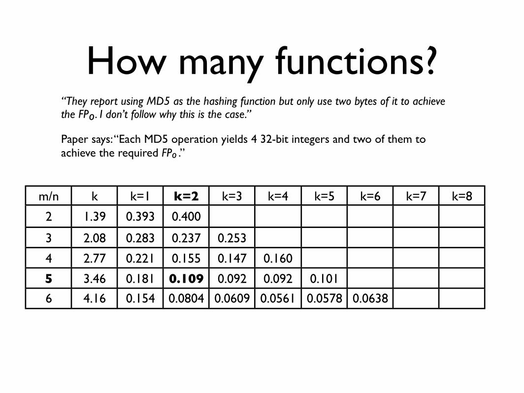
How many functions?“They report using MD5 as the hashing function but only use two bytes of it to achieve the FP . I don’t follow why this is the case.”
Paper says: “Each MD5 operation yields 4 32-bit integers and two of them to achieve the required FP .”
o
o
m/n k k=1 k=2 k=3 k=4 k=5 k=6 k=7 k=8
2 1.39 0.393 0.400
3 2.08 0.283 0.237 0.253
4 2.77 0.221 0.155 0.147 0.160
5 3.46 0.181 0.109 0.092 0.092 0.101
6 4.16 0.154 0.0804 0.0609 0.0561 0.0578 0.0638
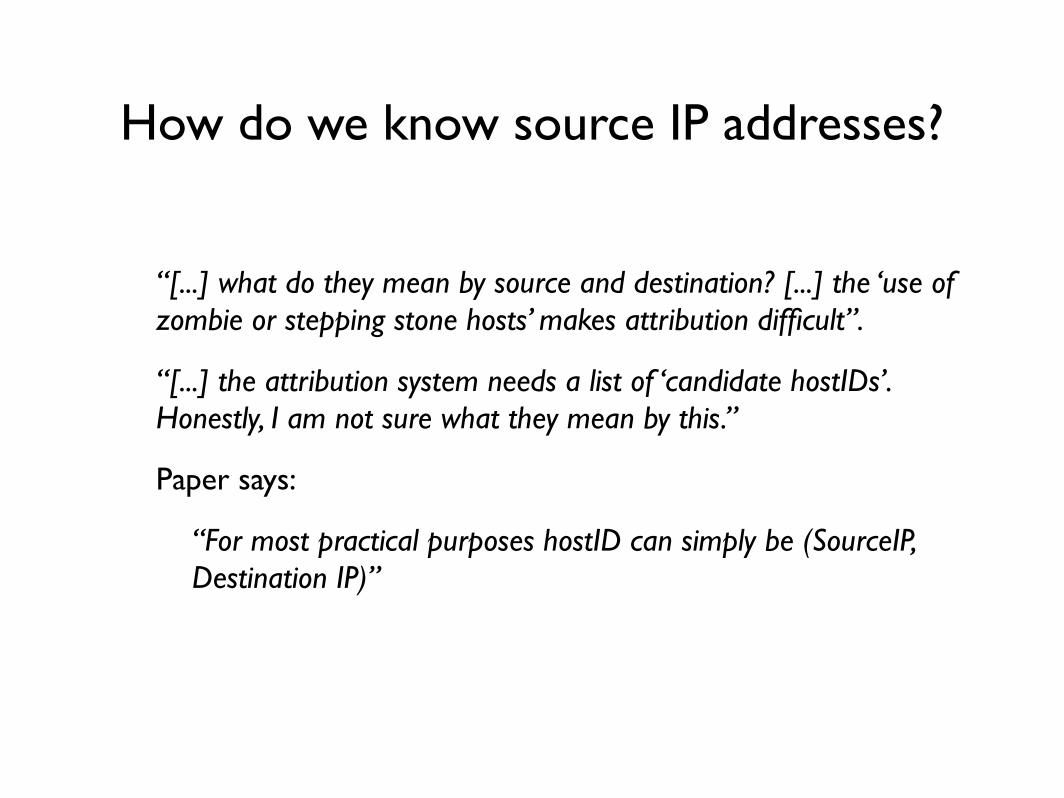
How do we know source IP addresses?
“[...] what do they mean by source and destination? [...] the ‘use of zombie or stepping stone hosts’ makes attribution difficult”.
“[...] the attribution system needs a list of ‘candidate hostIDs’. Honestly, I am not sure what they mean by this.”
Paper says:
“For most practical purposes hostID can simply be (SourceIP, Destination IP)”
More accuracy with block digest?
“The block digest is a HBF as all the others and the number of inserted values are the same as the offset digest. Why is then the accuracy better?”
The number of entries is the same but think about how you do a query? How is FP rate influenced by that?
Query time /space tradeoff(block digest)
“[...] such an extension (block digest) would shorten query times, but increase the storage requirement. What is the tradeoff between querying time and space storage?”
What payload attribution?(aka Spoofed addresses)
“I am unsure of the specific contribution that this paper makes. The authors purport to have a method for attributing payload to source, destinations pairs, yet the system itself has no properties that allow you to correlate a payload with a specific sender”.
What would you prefer: a system like this one or one which requires global deployment (like SPIE)?

Various comments
How do you find it?
“smart and simple”“quite ingenious with regard to storage and querying”“The authors seem to skip any analysis that doesn’t come up in the actual implementation.”
Fabian’s answer: “That’s fine :-)”
“seem to be a useful construction”“I thought this was a decent paper overall. [...] I think it is also poorly written and lacks a good number of details.”
“I liked this paper very much.”
Extensions
Ryan: “Large Batch Authentication”
Scott:Use a variable length block size (hm...)
Razvan: Save the space for hostIDs using a global IP list?
Jay’s crazy idea: Address the spoofed address problem using hop-count-filtering?
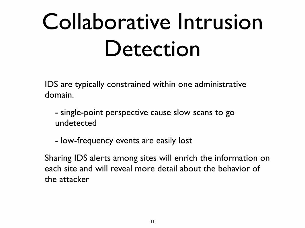
Collaborative Intrusion Detection
IDS are typically constrained within one administrative domain.
- single-point perspective cause slow scans to go undetected
- low-frequency events are easily lost
Sharing IDS alerts among sites will enrich the information on each site and will reveal more detail about the behavior of the attacker
11
Benefits
• Better understanding of the attacker intent
• Precise models of adversarial behavior
• Better view or global network attack activity
12
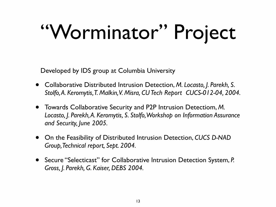
“Worminator” Project
Developed by IDS group at Columbia University
• Collaborative Distributed Intrusion Detection, M. Locasto, J. Parekh, S. Stolfo, A. Keromytis, T. Malkin, V. Misra, CU Tech Report CUCS-012-04, 2004.
• Towards Collaborative Security and P2P Intrusion Detectiom, M. Locasto, J. Parekh, A. Keromytis, S. Stolfo, Workshop on Information Assurance and Security, June 2005.
• On the Feasibility of Distributed Intrusion Detection, CUCS D-NAD Group, Technical report, Sept. 2004.
• Secure “Selecticast” for Collaborative Intrusion Detection System, P. Gross, J. Parekh, G. Kaiser, DEBS 2004.
13
Terminology
1. Network event
2. Alert
3. Sensor node
4. Correlation node
5. Threat assessment node
14
Challenges
• Large alert rates
• A centralized system to aggregate and correlate alert information is not feasible.
• Exchanging alert data in a full mesh quadratically increases bandwidth requirements
• If alert data is partitioned in distinct sets, some correlations may be lost
• Privacy considerations
15
Privacy Implications
Alerts may contain sensitive information: IP addresses, ports, protocol, timestamps etc.
Problem: Reveal internal topology, configurations, site vulnerabilities.
From here the idea of “anonymization”:
- Don’t reveal sensitive information
- Tradeoff between anonymity and utility
16
Assumptions
• Alerts from Snort
• Focus on detection of scanning and probing activity
• Integrity and confidentiality of exchange messages can be addressed with IPsec, TLS/SSL & friends
• Unless compromised, any participant provides entire alert information to others (they don’t disclose partial data)
17
Threat model
• Attacker attempts to evade the system by performing very low rate scans and probes
• Attacker can compromise a subset of nodes to discover information about the organization he is targeting
18
Bloom filtersto the Rescue
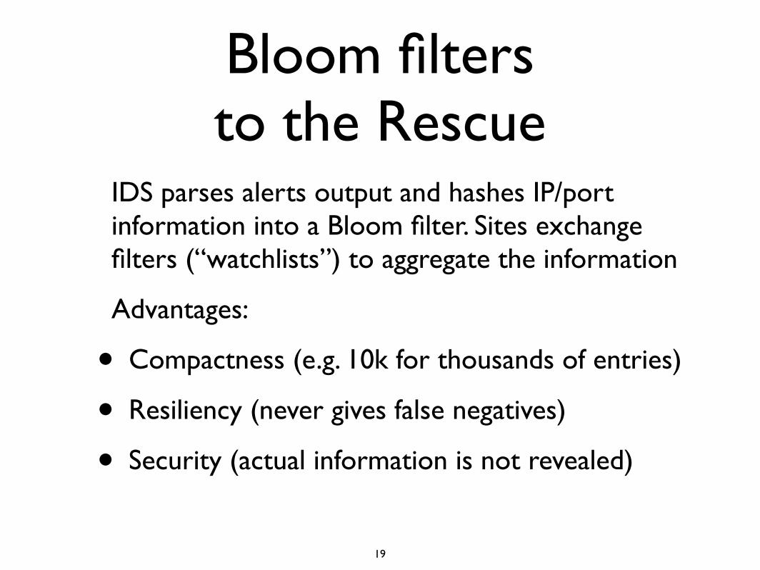
IDS parses alerts output and hashes IP/port information into a Bloom filter. Sites exchange filters (“watchlists”) to aggregate the information
Advantages:
• Compactness (e.g. 10k for thousands of entries)
• Resiliency (never gives false negatives)
• Security (actual information is not revealed)
19
Distributed correlation
1. Fully connected mesh
2. DHT
3. Dynamic overlay network
- Whirlpool
20
Approaches:
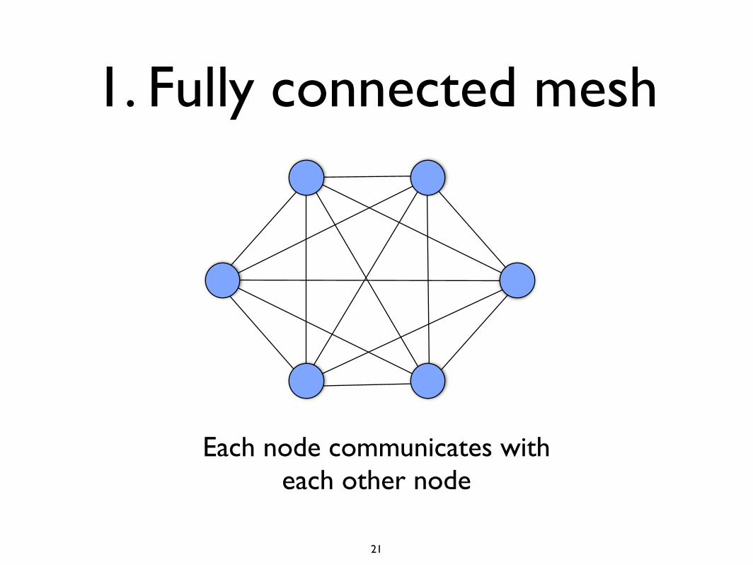
1. Fully connected mesh
Each node communicates with each other node
21
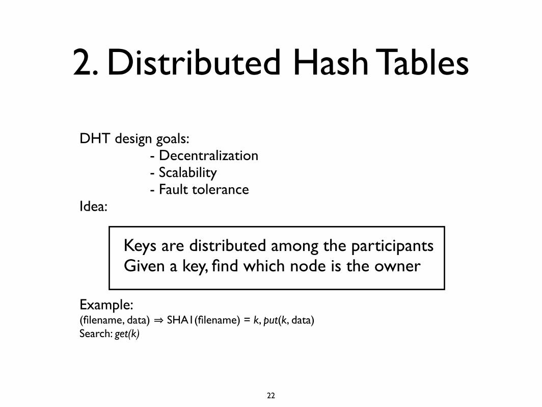
2. Distributed Hash Tables
DHT design goals: - Decentralization - Scalability - Fault toleranceIdea:
Keys are distributed among the participants Given a key, find which node is the owner
Example:(filename, data) ⇒ SHA1(filename) = k, put(k, data)Search: get(k)
22
Chord
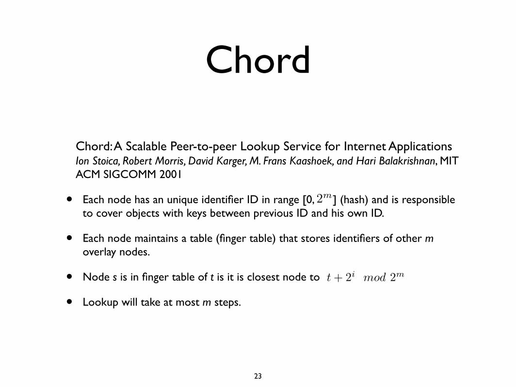
Chord: A Scalable Peer-to-peer Lookup Service for Internet ApplicationsIon Stoica, Robert Morris, David Karger, M. Frans Kaashoek, and Hari Balakrishnan, MITACM SIGCOMM 2001
• Each node has an unique identifier ID in range [0, ] (hash) and is responsible to cover objects with keys between previous ID and his own ID.
• Each node maintains a table (finger table) that stores identifiers of other m overlay nodes.
• Node s is in finger table of t is it is closest node to
• Lookup will take at most m steps.
2m
1
t + 2i mod 2m
1
23
Chord1
5
12
40
7
1918
25
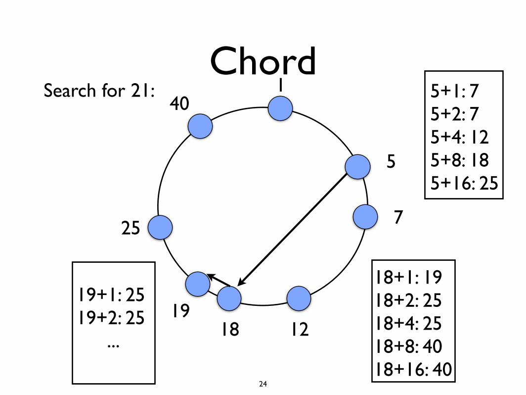
5+1: 75+2: 75+4: 125+8: 185+16: 25
18+1: 1918+2: 2518+4: 2518+8: 4018+16: 40
19+1: 2519+2: 25
...
Search for 21:
24
DHT for correlations
Map alert data (IP addresses, ports) to correlation nodes.
Limitations:
• nodes are single point of failure for specific IPs
• too much trust in a single node (collects highly related information at one node)
25
Dynamic Overlay Networks
Idea: Use a dynamic mapping between the nodes and content.
Requirement: Need to have the correct subset of nodes that must communicate given a particular alert.
There is a theoretical optimal schedule for communication information (correct subsets are always communicating).
Naive solution: pick relationships at random.
26

Whirlpool
Mechanism for coordinating the exchange of information between the members of a correlation group.
Approximates “optimal” scheduler by using a mechanism which allows a good balance between traffic exchange and information loss.
27
Whirlpool
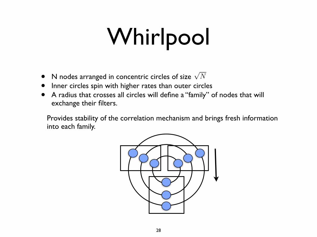
• N nodes arranged in concentric circles of size
• Inner circles spin with higher rates than outer circles
• A radius that crosses all circles will define a “family” of nodes that will exchange their filters.
Provides stability of the correlation mechanism and brings fresh information into each family.
28
Multihome Routing in Wireless Mesh Network with
Fast Handoff
Abstract—This paper presents the multihome routing proto-cols of a wireless mesh system that offers intra-domain and inter-domain handoff with real-time performance. The system consistsof several access points where some are connected to the Internet
while others rely on multi-hop wireless communication. Internetand peer-to-peer communication take advantage of wired con-nections to minimize the number of wireless transmissions. NewInternet connected flows use the closest Internet connected accesspoint, while existing flows are forwarded using the wired networkto their original wired connected access point, to maintainexternal connectivity. The wireless mesh network provides fasthandoff, supporting VoIP and other real-time application traffic.Continuous Internet connectivity and real-time response duringhandoffs is maintained by using an overlay network betweenwireless access points. During handoff transitions, our systemensures that the Internet flows are routed through at least oneInternet connected access point at any time.
I. INTRODUCTION√
N Despite an extensive body of research in multi-hop
wireless routing, most of the Wi-Fi connectivity today resem-
bles the use of a cordless phone; a mobile device, e.g. laptop,
connects to an access point, which relays the communication
either to remote devices, via a wired infrastructure, or to other
wireless devices that are located in the range of the access
point. Wireless mesh networks provide a promising paradigm
to increase the mobility range of wireless devices by extending
the coverage area to more than the range of a single access
point. They use muliple access points that create a mesh
topology and forward packets using multiple wireless hops.
Some of the access points may be connected to the Internet,
while others may not. We say that a wireless mesh network is
multihomed if more than one access point in the topology is
connected to the Internet with a wired link.
Wireless mesh networks are usually self-organizing, easily
deployable, and therefore are useful for providing peer-to-peer
and Internet connectivity in remote geographical areas or for
first responders in disaster affected areas that lack the wired
infrastructure. In such scenarios, providing support for real-
time applications such as VoIP is often critical.
While the access points are usually static, mobile devices
that connect to the mesh network can roam throughout the cov-
erage area and require both peer-to-peer and external, Internet
connectivity. In a multihomed mesh network efficient routing
protocols are required to use the wired connectivity as much as
possible to reduce the number of wireless transmissions and to
forward packets to the closest Internet connected Access point.
The challenge resides in maintaining existing connections as
a mobile device moves closer to a different wired access
point, allowing packets to flow with real-time response, and
minimizing the usage of wireless hops, even during the times
when access points are changed.
This paper presents a practical handoff routing protocol
for multihomed wireless mesh networks that maintains real-
time characteristics of traffic such as VoIP, even when mobile
clients move closer to a different wired connected accass
point. Continue the paragraph with technical details of
the approach.
We implemented our approach in a wireless mesh net-
work prototype and deployed it over three buildings in a
university campus, providing daily Internet connectivity to
multiple users. Experimental results on our testbed show that...
Continue the paragraph with performance resullts.
The main contribution of this work are:
• A fast handoff protocol for multihomed wireless mesh
networks that supports real-time applications such as
VoIP.
• A routing mechanism that integrates seamlessly both
wired and wireless connectivity in multihomed mesh
networks.
• A routing protocol for mesh peer-to-peer communication
that optimizes the number hops in inter-domain commu-
nication.
The rest of the paper is organized as follows: Section II
presents related work. In Section III we describe the archi-
tecture of our multihomed mesh network approach, and in
Section IV we present the real-time handoff routing protocol
between the wired connected access points. Experimental
results are presented in Section V, and Section VI concludes
the paper.
II. RELATED WORK
One of the first approaches to provide mobile connectivity
while moving between different wireless domains was Mobile
IP [1], [2]. The approach preserves a permanent home IP
address for each mobile client, bound by an agent at its home
domain. As the mobile client moves to a different network
domain it receives a Care-of-Address (CoA) from an agent
in the foreign network. The mobile client then registers its
new address with its home agent, and tunnels all its data
through the home agent. This approach is useful for clients
that are mostly located in a home domain, and occasionally
move to other domains, otherwise it may result in an inefficient
path of the packets. Several improvements have been proposed
to cope with this problem [][]. However, in the general case
Mobile IP does not provide a real-time handoff and can use
more hops than the optimal routing solution. For example, two
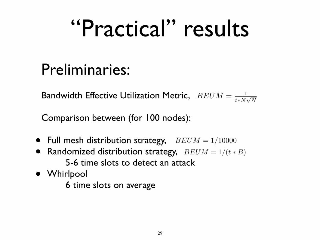
“Practical” results
Preliminaries:
Bandwidth Effective Utilization Metric,
Comparison between (for 100 nodes):
• Full mesh distribution strategy,
• Randomized distribution strategy, 5-6 time slots to detect an attack
• Whirlpool 6 time slots on average
29
t + 2i mod 2m BEUM = 1
t∗N√
N
1
t + 2i mod 2m
BEUM =1
t ∗ N√
N
BEUM = 1/(t ∗ B)
BEUM = 1/10000
1
t + 2i mod 2m
BEUM =1
t ∗ N√
N
BEUM = 1/(t ∗ B)
BEUM = 1/10000
1
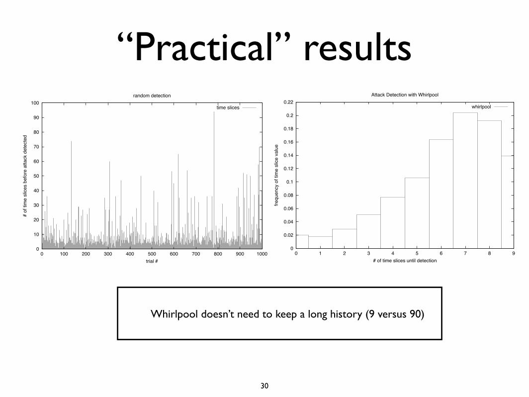
“Practical” results
Whirlpool doesn’t need to keep a long history (9 versus 90)
30
0
10
20
30
40
50
60
70
80
90
100
0 100 200 300 400 500 600 700 800 900 1000
# o
f tim
e s
lices b
efo
re a
ttack d
ete
cte
d
trial #
random detection
time slices
Figure 4: Number of time slices until random distribution detects an attack. The average numberfor this particular data plot is 6 time slices.
same output is intended for all parties). The crucial point is that the protocol must be secure evenwhen an adversary controls the actions of some of the parties. In particular, the output should becomputed correctly, and privacy of the inputs should be maintained: no information should leak toany party, beyond what inevitably follows from seeing their own input and output.The full definition of security for such a protocol is quite complex, and we do not detail it here.
However, we note that the definition is based on a comparison to an ”ideal model”, where there isa centralized trusted entity with a secure connection to each of the parties, who can compute thefunction for them and deliver the output securely (clearly such a fully trusted party does not exist inthe real world). A protocol is considered secure, if there is nothing that an attacker can achieve byattacking the protocol in the real world, beyond what could be done in the ideal world (essentially,nothing).One of the most celebrated results in cryptography, is that in fact any function that can be
computed, can be computed securely, assuming at most one third of the parties are compromised.4This is a very general result , allowing to secure any protocol. The overhead may be prohibitive,depending on the context where the technique is employed, and we address this issue below.We next discuss the advantages gained by using secure multi-party computation techniques in
our context, namely robustness and privacy.4There are several other flavors of this result. For example, it holds even when up to half the parties are compro-
mised, provided there is a broadcast channel.
19
0
0.02
0.04
0.06
0.08
0.1
0.12
0.14
0.16
0.18
0.2
0.22
0 1 2 3 4 5 6 7 8 9
fre
qu
en
cy o
f tim
e s
lice
va
lue
# of time slices until detection
Attack Detection with Whirlpool
whirlpool
Figure 5: The number of time slices to detect an attack with Whirlpool over 1000 trials. For thisgraph, the average number of time slices was 6. This is not surprising, since the Whirlpool is aspecial case of a random schedule. Note, however, that Whirlpool does not have the outliers that arandom schedule has because it converges.
ROBUSTNESS. Reliability of the system must be maintained in the presence of accidentalfailures and malicious attacks. As we explained above, reliability against accidental failures isachieved by designing our system in a fault tolerant way, using self-healing systems. Further, toprotect malicious attacks on the network, strong cryptography (e.g., TLS) can be used to assureauthenticity and integrity of the data sent. However, these methods are not sufficient if actual nodesare compromised together with all their pertaining secret key material, which is made available to amalicious attacker. In this case, secure multi-party computation can be used, under the assumptionthat no more than one third of all nodes are compromised in this strong way. The resulting protocolassures that no matter how the compromised nodes behave, they cannot disrupt the computation(e.g., they cannot thwart the outputted correlated list).PRIVACY. Another important advantage of secure multi-party computation, is that of main-
taining privacy of the data. Indeed, when the communicating nodes wish to correlate their data tocreate alerts, it is often desirable that the data is not leaked to other participating nodes, beyondthe unavoidable information that can be obtained from the outcome of the computation, such asthe watchlist. The distributed nature of our system, as well as our use of Bloom filters and datareduction mechanisms, already facilitate some amount of privacy, as compared to the centralizedor full-mesh communication solutions. If higher degree of privacy is desired, secure multi-partycomputation assures privacy to the highest possible degree, namely a proof that no information
20
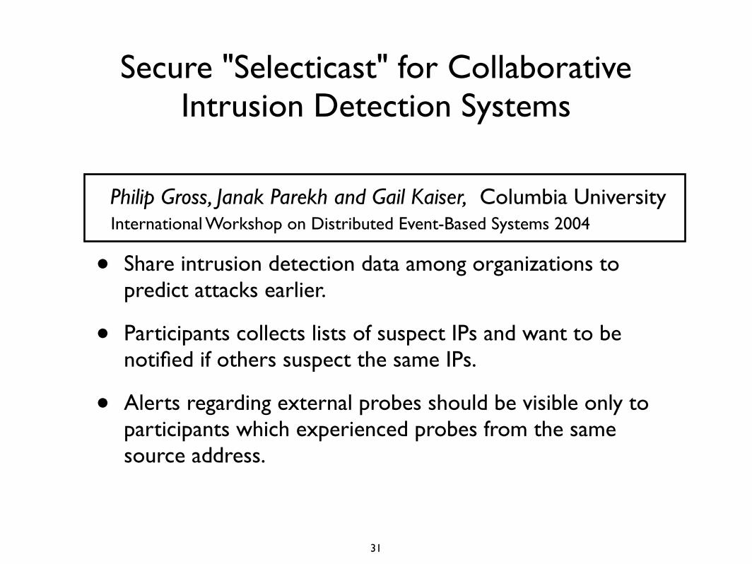
Secure "Selecticast" for Collaborative Intrusion Detection Systems
Philip Gross, Janak Parekh and Gail Kaiser, Columbia University International Workshop on Distributed Event-Based Systems 2004
• Share intrusion detection data among organizations to predict attacks earlier.
• Participants collects lists of suspect IPs and want to be notified if others suspect the same IPs.
• Alerts regarding external probes should be visible only to participants which experienced probes from the same source address.
31
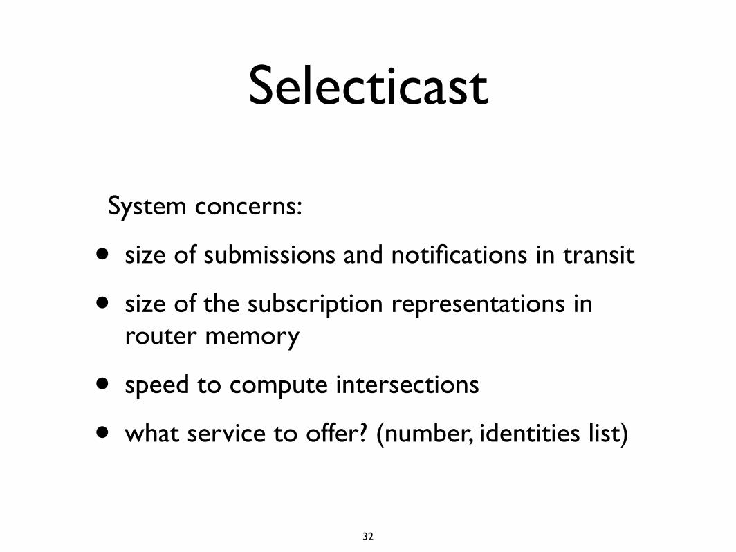
Selecticast
System concerns:
• size of submissions and notifications in transit
• size of the subscription representations in router memory
• speed to compute intersections
• what service to offer? (number, identities list)
32
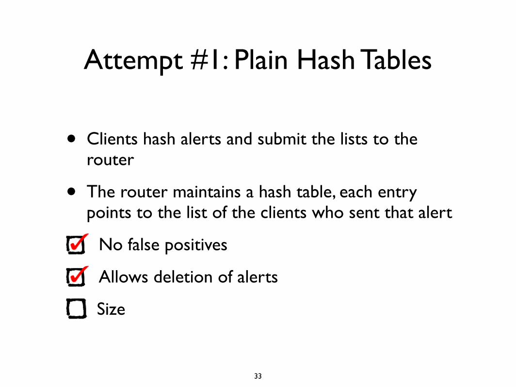
Attempt #1: Plain Hash Tables
• Clients hash alerts and submit the lists to the router
• The router maintains a hash table, each entry points to the list of the clients who sent that alert
No false positives
Allows deletion of alerts
Size
33
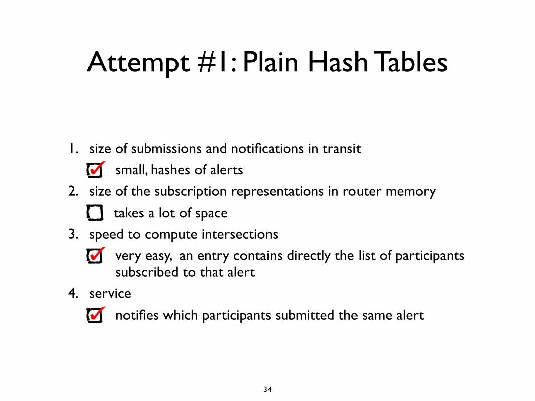
Attempt #1: Plain Hash Tables
1. size of submissions and notifications in transit
small, hashes of alerts
2. size of the subscription representations in router memory
takes a lot of space
3. speed to compute intersections
very easy, an entry contains directly the list of participants subscribed to that alert
4. service
notifies which participants submitted the same alert
34
Attempt #2: Pure Bloom Filters
• Clients submit a Bloom filter representing their alerts
• How does the router look for matches?
35

Attempt #2: Pure Bloom Filters
Bloom filter of size m storing n distinct values, k bits per item.
A bit is set with probability p =
One bit matches a bit from the other filter is a Bernoulli trial with chance of success p.
Expected number of successes in kn trials is knp
Ex:
Problem: it will require 7000+ bits/item !!!
!
"#$$%&'!('!)*+'! ,(%!-.%%/! 01.,'2&!%0! &13'!m! 41,&5! '*6)!
&,%2178!n!91&,176,!+*.#'&!:1;';5!7%!+*.#'&!17!6%//%7<!#&178!
k! 41,&! $'2! 1,'/;! ! =! 41,! 17! ,)'! 01.,'2! (1..! 4'! &',! (1,)!
$2%4*41.1,>!p5!2%#8).>! ! "knm??? ## ;!!@%2!%$,1/*.!-.%%/!
01.,'2&5! p! &)%#.9! 4'! 7'*2! A;B5! *.,)%#8)! ('! 6*7! /*C'! 1,!
/#6)!&$*2&'2!*,!,)'!6%&,!%0!1762'*&'9!/'/%2>!#&*8';!!!
@%2!%#2!6*7919*,'!-.%%/!01.,'25!('!6*7!+1'(!,)'!6*&'!
,)*,!%7'!%0!%#2!41,&!6%17619'7,.>!/*,6)'&!*!41,!17!,)'!%,)'2!
01.,'2!*&!*!-'27%#..1!,21*.!(1,)!6)*76'!%0!DB'&&E!p;!!F)'!
7#/4'2! %0! /*,6)178! 41,&! (1..! ,)'7! 0%..%(! *! 417%/1*.!
91&,214#,1%75!(1,)!,)'!'G$'6,'9!7#/4'2!%0!B'&&'&!17!kn!
,21*.&! 'H#*.! ,%! knp;! ! I%/$#,'2! &1/#.*,1%7! 6%7012/&! ,)'!
*66#2*6>!%0!,)1&!*7*.>&1&;!!knp!(1..!4'!+*&,.>!82'*,'2!,)*7!
k5! *79! ,)#&! ,)'! 7#/4'2! %0! 0*.&'! $%&1,1+'&! (1..! 4'!
'7%2/%#&;! ! J+'7! 10! ('! ,2>! ,%! .%('2! knp! 4>! /*C178! p!
'G,2'/'.>!&/*..!:*79!/*C178!,)'!01.,'2!'G,2'/'.>!&$*2&'<5!
.*28'! +*.#'&! %0! n! (1..! 2*$19.>! /*C'! ,)'! &1,#*,1%7!
#7(%2C*4.';!!!
@%2!17&,*76'5!10!k!1&!K5!*79!,)#&!('!(*7,!%#2!'G$'6,'9!
7#/4'2!%0!6%..1&1%7&!,%!4'!.'&&!,)*7!K5!('!/#&,!$#,!0'('2!
,)*7!?LAA!1,'/&!17,%!*7!M!/1..1%7!41,!:?N-<!-.%%/!01.,'2!
:kOK5!nO??MP5!mOLLP5!p!A;AAAM5!knp!K;A<;!!Q%,'!,)*,!,)1&!
6%&,! 1&! %7.>! 176#22'9! 17!/'/%2>;! !R'! 6*7! 6%/$2'&&! ,)'!
01.,'2!9#2178!7',(%2C!,2*7&/1&&1%7!4>!*!.*28'!0*6,%2!#&178!
&,*79*29!6%/$2'&&1%7!,%%.&;!!Q%7',)'.'&&5!*79!'+'7!81+'7!
,)'!&$''9!%0!&1/$.>!=QS178!,)'!,(%!.*28'!-.%%/!01.,'2&!
,%8',)'25! TAAAU! 41,&! $'2! 1,'/! &,%2'9! 1&! *! )18).>!
#7*,,2*6,1+'!2*,1%;!
!
Hybrid Bloom Filter
R'! 6*7! B'&&0#..>! .'+'2*8'! ,)'! &13'! *9+*7,*8'! %0!
-.%%/! 01.,'2&! 4>! 6%/417178! ,)'/! (1,)! ,)'! &',V%0V)*&)V
+*.#'&! *$$2%*6);! ! W*2,161$*7,&! /1,! ,)'! .1&,! %0! )*&)!
+*.#'&! %0! 17,'2'&,5! 2'$2'&'7,178! 7%,'9! 17&,*76'&! %0!
&#&$161%#&! 7',(%2C! *6,1+1,>;! ! F)'! 2%#,'2! #&'&! ,)'! *6,#*.!
)*&)!+*.#'&!,%!6)'6C!*8*17&,!,)'!-.%%/!01.,'2&!%0!,)'!%,)'2!
$*2,161$*7,&!,%!0179!/*,6)'&!(1,)!2'*&%7*4.'!*66#2*6>;!!X0!
/*,6)'&! *2'! 0%#795! ,)'! 2%#,'2! &'79&! ,)'!/*,6)178!+*.#'&!
*&! *! 7%,1016*,1%7! ,%! *..! /*,6)178! $*2,161$*7,&;!!
=991,1%7*..>5!,)'!2%#,'2!6%7+'2,&!,)'!/1,,'9!&',!%0!)*&)!
+*.#'&!17,%!*!-.%%/!01.,'2!%0!&13'! nYM !41,&5!()'2'! nY !1&!,)'!
'&,1/*,'9! ,%,*.!7#/4'2!%0!+*.#'&!$'2!$*2,161$*7,!:/*C178!
*..! 01.,'2&! ,)'! &*/'! &13'5! *79! 81+178! *! 6)*76'! %0! 0*.&'!
$%&1,1+'! *2%#79! LZ<;! ! F)1&! 01.,'2! 1&! ,)'7! &,%2'9! *79!
*&&%61*,'9!(1,)! ,)'!/1,,'2;! !=0,'2!*..!%0! ,)'!/1,,'9!
)*&)! +*.#'&! )*+'! 4''7! 6)'6C'9! *8*17&,! '+'2>%7'! '.&'[&!
-.%%/! 01.,'2&5! ,)'! 2%#,'2! 6*7! ,)'7! 91&6*29! ,)'! /1,,'9!
)*&)! +*.#'! .1&,5! .'*+178! %7.>! ,)'! &6214'2[&! :/#6)!
&/*..'2<!-.%%/!01.,'2;!!!
F)#&! $#4.1&)'2&! /1,! .*28'! &',&! %0! )*&)! +*.#'&5!
()16)! *2'! #&'9! ,%! 0179! /*,6)'&5! *79! ,)'7! .'*+'! 4')179!
/#6)! &/*..'2! -.%%/! 01.,'2! D2'&19#'&E! ,)*,! *6,! *&!
&621$,1%7&;! ! N*,6)178! )*&)! +*.#'! &',&! :%$,1%7*..>!
,*88'9!(1,)!,)'!19'7,1,>!%0!,)'12!/1,,'2<!*2'!&'7,!%#,!*&!
,)'!*6,#*.!7%,1016*,1%7&;!!@%2!,)1&!9%/*175!('!*&&#/'!,)*,!
,)'!7#/4'2!%0!7%,1016*,1%7&!1&!+'2>!&/*..!17!2'.*,1%7!,%!,)'!
7#/4'2! %0! +*.#'&! /1,,'9! :'G$'21/'7,&! &)%(!
6%22'.*,1%7! 2*,'&! %0! A;A?Z! %2! .%('2<;! ! X0! ,)'! 7#/4'2! %0!
/*,6)'&! 1&!'G$'6,'9! ,%!4'! .*28'5! ,)'!/*,6)178!&',&!6%#.9!
,)'/&'.+'&! 4'! 6%7+'2,'9! ,%! -.%%/! 01.,'2&! 4'0%2'! 4'178!
&'7,!*&!7%,1016*,1%7&5!(1,)!,)'!*,,'79*7,!&$*6'!&*+178&;!!!
Q%,'! ,)*,! ,)'! )*&)! +*.#'&! #&'9! 0%2! -.%%/! 01.,'2!
8'7'2*,1%7!*2'!/#6)!.*28'2!,)*7!,)'!)*&)!+*.#'&!#&'9!4>!*!
$.*17!)*&),*4.'5!'+'7! ,)%#8)! ,)'! 2'&#.,178! 01.,'2!&,2#6,#2'!
1&! &/*..'2! ,)*7! ,)'! 6%22'&$%79178! )*&),*4.';! ! @%2! '*6)!
1,'/! '7,'2'95! -.%%/! 01.,'2&! 7''9! k! 17916'&! 17,%! *7!mV41,!
,*4.'5! *79! ,)#&! *! ,%,*.! %0!k.7m! 41,&! %0! )*&)!$'2! 1,'/;! ! X0!
mOMn5! ,)'7! k:PU.7n<! 41,&;! ! @%2! &',&! %0! L5AAA! ,%! ?LM5AAA!
1,'/&!*79!COK5!,)1&!(%2C&!%#,!,%!M\V?LA!41,&!$'2!1,'/5!%2!*!
0*6,%2! %0! PV\! 1762'*&'! %+'2! ,)'! &13'! %0! ,)'! )*&)! +*.#'&!
7''9'9!0%2!$.*17!)*&),*4.'&;!!F)1&!(%#.9!$%,'7,1*..>!4'!*!
$2%4.'/!0%2!,)'!/1&&1%7!%0!.*28'!&',&!%0!)*&)'9!+*.#'&!
17!,)'!)>4219!6*&';!
]%('+'25!('! 6*7! *+%19! ,)1&! $2%4.'/!4>!)*&)178!%#2!
*.'2,&!,%!PL!41,&!0%2!,2*7&/1&&1%75!*79!,)'7!2')*&)178!'*6)!
,%!?LAU!41,&!*0,'2!1,!*221+'&!*,!,)'!&'2+'2!:*79!,)'7!&$.1,,178!
#$!,)%&'!41,&!17,%!,)'!C!17916'&!%0!&13'!.7m!,)*,!('!7''9<5!
,)#&!/*C178!,)'!,2*7&/1&&1%7!6%&,!7%!/%2'!'G$'7&1+'!,)*7!
0%2! $.*17! )*&),*4.'&;! ! "176'! ,)'! %21817*.! *.'2,&! (1..!
,>$16*..>! 6%7,*17! .'&&! ,)*7! PL! 41,&! %0! '7,2%$>5! 7%!
170%2/*,1%7! &)%#.9! 4'! .%&,! (1,)! ,)1&! ,(%V&,*8'! )*&)178!
$2%6'&&;!
!
Optimization with Two-Stage Compare
X7! ,)'! )>4219! 6*&'! 9'&6214'9! *4%+'5!('! *&&#/'9! ,)*,!
,)'! 2%#,'2!/*17,*17&! *! &'$*2*,'! -.%%/! 01.,'2! 0%2! '*6)! %0!
,)'!C!6%..*4%2*,178!$*2,1'&5!2'$2'&'7,178!,)'!&$'61016!&',!%0!
*.'2,&! &''7! 4>! ,)*,! $*2,>;! !R)'7! *! 7'(! &',! %0! +*.#'&! 1&!
$#4.1&)'95! 1,!/#&,! 4'! 6%/$*2'9! *8*17&,! '*6)! %0! ,)'!C-1!
%,)'2!&',&;!!R'!6*7!&$''9!$2%6'&&178!4>!'7,'2178!*..!%0!,)'!
/1,,'9! +*.#'! &',&! 17,%! *! &178.'! .*28'! D/*&,'2E!-.%%/!
01.,'2!17!,)'!^%#,'2!*79!6)'6C178!,)1&!012&,;!!!
X0!('!0179!*!/*,6)!17!,)'!/*&,'2!-.%%/!01.,'25!('!/#&,!
,)'7! 6)'6C! '*6)! 1791+19#*.! 01.,'2! ,%!91&6%+'2! ,)'! &$'61016!
$*2,161$*7,&! ()%! /*,6)'9;! ! S'&$1,'! ,)1&5! ('! (1..! &)%(!
,)*,!,)1&!*$$2%*6)!6*7!%00'2!&,*7,1*.!&$*6'!'00161'761'&!
%+'2!,)'!)*&)!,*4.'!*$$2%*6)5!*79!,)'!&$''9!91&*9+*7,*8'!
6*7!4'!2'9#6'9;!
R'! 6*7! &$''9! %#2! -.%%/! 01.,'2! .%%C#$&! 4>! ,*C178!
*9+*7,*8'! %0! *21,)/',16! /%9#.%! Lm! %7! 417*2>! 7#/4'2&;!!
_#&,! *&! *! 4*&'! ?A! 7#/4'2! /%9#.%! ?Am! 1&! ,)'! .'*&,!
&1871016*7,! m! 9181,&! %0! ,)'! 7#/4'25! *! 417*2>! 7#/4'2!
/%9#.%!Lm!1&!`#&,!,)'!4%,,%/!m!41,&!%0!,)'!7#/4'25!()16)!
6*7! 4'! 'G,2*6,'9! 4>! =QS178! ,)'! 7#/4'2! (1,)! *7!
*$$2%$21*,'! 41,! /*&C! :(1<<m)–1! #&178! ,)'! IV.*78#*8'!
41,!%$'2*,%2&<;!
a',!n’!4'!,)'!$%('2!%0!L!6.%&'&,!,%!n;! !R'!62'*,'!%7'!
/*&,'2!-.%%/!01.,'2!%0!&13'!Cn’!*79!*!01.,'2!%0!&13'!n’!0%2!
'*6)!%0!,)'!C!$*2,161$*7,&;!!"13178!,)'&'!*,!M!41,&!$'2!1,'/5!
!
"#$$%&'!('!)*+'! ,(%!-.%%/! 01.,'2&!%0! &13'!m! 41,&5! '*6)!
&,%2178!n!91&,176,!+*.#'&!:1;';5!7%!+*.#'&!17!6%//%7<!#&178!
k! 41,&! $'2! 1,'/;! ! =! 41,! 17! ,)'! 01.,'2! (1..! 4'! &',! (1,)!
$2%4*41.1,>!p5!2%#8).>! ! "knm??? ## ;!!@%2!%$,1/*.!-.%%/!
01.,'2&5! p! &)%#.9! 4'! 7'*2! A;B5! *.,)%#8)! ('! 6*7! /*C'! 1,!
/#6)!&$*2&'2!*,!,)'!6%&,!%0!1762'*&'9!/'/%2>!#&*8';!!!
@%2!%#2!6*7919*,'!-.%%/!01.,'25!('!6*7!+1'(!,)'!6*&'!
,)*,!%7'!%0!%#2!41,&!6%17619'7,.>!/*,6)'&!*!41,!17!,)'!%,)'2!
01.,'2!*&!*!-'27%#..1!,21*.!(1,)!6)*76'!%0!DB'&&E!p;!!F)'!
7#/4'2! %0! /*,6)178! 41,&! (1..! ,)'7! 0%..%(! *! 417%/1*.!
91&,214#,1%75!(1,)!,)'!'G$'6,'9!7#/4'2!%0!B'&&'&!17!kn!
,21*.&! 'H#*.! ,%! knp;! ! I%/$#,'2! &1/#.*,1%7! 6%7012/&! ,)'!
*66#2*6>!%0!,)1&!*7*.>&1&;!!knp!(1..!4'!+*&,.>!82'*,'2!,)*7!
k5! *79! ,)#&! ,)'! 7#/4'2! %0! 0*.&'! $%&1,1+'&! (1..! 4'!
'7%2/%#&;! ! J+'7! 10! ('! ,2>! ,%! .%('2! knp! 4>! /*C178! p!
'G,2'/'.>!&/*..!:*79!/*C178!,)'!01.,'2!'G,2'/'.>!&$*2&'<5!
.*28'! +*.#'&! %0! n! (1..! 2*$19.>! /*C'! ,)'! &1,#*,1%7!
#7(%2C*4.';!!!
@%2!17&,*76'5!10!k!1&!K5!*79!,)#&!('!(*7,!%#2!'G$'6,'9!
7#/4'2!%0!6%..1&1%7&!,%!4'!.'&&!,)*7!K5!('!/#&,!$#,!0'('2!
,)*7!?LAA!1,'/&!17,%!*7!M!/1..1%7!41,!:?N-<!-.%%/!01.,'2!
:kOK5!nO??MP5!mOLLP5!p!A;AAAM5!knp!K;A<;!!Q%,'!,)*,!,)1&!
6%&,! 1&! %7.>! 176#22'9! 17!/'/%2>;! !R'! 6*7! 6%/$2'&&! ,)'!
01.,'2!9#2178!7',(%2C!,2*7&/1&&1%7!4>!*!.*28'!0*6,%2!#&178!
&,*79*29!6%/$2'&&1%7!,%%.&;!!Q%7',)'.'&&5!*79!'+'7!81+'7!
,)'!&$''9!%0!&1/$.>!=QS178!,)'!,(%!.*28'!-.%%/!01.,'2&!
,%8',)'25! TAAAU! 41,&! $'2! 1,'/! &,%2'9! 1&! *! )18).>!
#7*,,2*6,1+'!2*,1%;!
!
Hybrid Bloom Filter
R'! 6*7! B'&&0#..>! .'+'2*8'! ,)'! &13'! *9+*7,*8'! %0!
-.%%/! 01.,'2&! 4>! 6%/417178! ,)'/! (1,)! ,)'! &',V%0V)*&)V
+*.#'&! *$$2%*6);! ! W*2,161$*7,&! /1,! ,)'! .1&,! %0! )*&)!
+*.#'&! %0! 17,'2'&,5! 2'$2'&'7,178! 7%,'9! 17&,*76'&! %0!
&#&$161%#&! 7',(%2C! *6,1+1,>;! ! F)'! 2%#,'2! #&'&! ,)'! *6,#*.!
)*&)!+*.#'&!,%!6)'6C!*8*17&,!,)'!-.%%/!01.,'2&!%0!,)'!%,)'2!
$*2,161$*7,&!,%!0179!/*,6)'&!(1,)!2'*&%7*4.'!*66#2*6>;!!X0!
/*,6)'&! *2'! 0%#795! ,)'! 2%#,'2! &'79&! ,)'!/*,6)178!+*.#'&!
*&! *! 7%,1016*,1%7! ,%! *..! /*,6)178! $*2,161$*7,&;!!
=991,1%7*..>5!,)'!2%#,'2!6%7+'2,&!,)'!/1,,'9!&',!%0!)*&)!
+*.#'&!17,%!*!-.%%/!01.,'2!%0!&13'! nYM !41,&5!()'2'! nY !1&!,)'!
'&,1/*,'9! ,%,*.!7#/4'2!%0!+*.#'&!$'2!$*2,161$*7,!:/*C178!
*..! 01.,'2&! ,)'! &*/'! &13'5! *79! 81+178! *! 6)*76'! %0! 0*.&'!
$%&1,1+'! *2%#79! LZ<;! ! F)1&! 01.,'2! 1&! ,)'7! &,%2'9! *79!
*&&%61*,'9!(1,)! ,)'!/1,,'2;! !=0,'2!*..!%0! ,)'!/1,,'9!
)*&)! +*.#'&! )*+'! 4''7! 6)'6C'9! *8*17&,! '+'2>%7'! '.&'[&!
-.%%/! 01.,'2&5! ,)'! 2%#,'2! 6*7! ,)'7! 91&6*29! ,)'! /1,,'9!
)*&)! +*.#'! .1&,5! .'*+178! %7.>! ,)'! &6214'2[&! :/#6)!
&/*..'2<!-.%%/!01.,'2;!!!
F)#&! $#4.1&)'2&! /1,! .*28'! &',&! %0! )*&)! +*.#'&5!
()16)! *2'! #&'9! ,%! 0179! /*,6)'&5! *79! ,)'7! .'*+'! 4')179!
/#6)! &/*..'2! -.%%/! 01.,'2! D2'&19#'&E! ,)*,! *6,! *&!
&621$,1%7&;! ! N*,6)178! )*&)! +*.#'! &',&! :%$,1%7*..>!
,*88'9!(1,)!,)'!19'7,1,>!%0!,)'12!/1,,'2<!*2'!&'7,!%#,!*&!
,)'!*6,#*.!7%,1016*,1%7&;!!@%2!,)1&!9%/*175!('!*&&#/'!,)*,!
,)'!7#/4'2!%0!7%,1016*,1%7&!1&!+'2>!&/*..!17!2'.*,1%7!,%!,)'!
7#/4'2! %0! +*.#'&! /1,,'9! :'G$'21/'7,&! &)%(!
6%22'.*,1%7! 2*,'&! %0! A;A?Z! %2! .%('2<;! ! X0! ,)'! 7#/4'2! %0!
/*,6)'&! 1&!'G$'6,'9! ,%!4'! .*28'5! ,)'!/*,6)178!&',&!6%#.9!
,)'/&'.+'&! 4'! 6%7+'2,'9! ,%! -.%%/! 01.,'2&! 4'0%2'! 4'178!
&'7,!*&!7%,1016*,1%7&5!(1,)!,)'!*,,'79*7,!&$*6'!&*+178&;!!!
Q%,'! ,)*,! ,)'! )*&)! +*.#'&! #&'9! 0%2! -.%%/! 01.,'2!
8'7'2*,1%7!*2'!/#6)!.*28'2!,)*7!,)'!)*&)!+*.#'&!#&'9!4>!*!
$.*17!)*&),*4.'5!'+'7! ,)%#8)! ,)'! 2'&#.,178! 01.,'2!&,2#6,#2'!
1&! &/*..'2! ,)*7! ,)'! 6%22'&$%79178! )*&),*4.';! ! @%2! '*6)!
1,'/! '7,'2'95! -.%%/! 01.,'2&! 7''9! k! 17916'&! 17,%! *7!mV41,!
,*4.'5! *79! ,)#&! *! ,%,*.! %0!k.7m! 41,&! %0! )*&)!$'2! 1,'/;! ! X0!
mOMn5! ,)'7! k:PU.7n<! 41,&;! ! @%2! &',&! %0! L5AAA! ,%! ?LM5AAA!
1,'/&!*79!COK5!,)1&!(%2C&!%#,!,%!M\V?LA!41,&!$'2!1,'/5!%2!*!
0*6,%2! %0! PV\! 1762'*&'! %+'2! ,)'! &13'! %0! ,)'! )*&)! +*.#'&!
7''9'9!0%2!$.*17!)*&),*4.'&;!!F)1&!(%#.9!$%,'7,1*..>!4'!*!
$2%4.'/!0%2!,)'!/1&&1%7!%0!.*28'!&',&!%0!)*&)'9!+*.#'&!
17!,)'!)>4219!6*&';!
]%('+'25!('! 6*7! *+%19! ,)1&! $2%4.'/!4>!)*&)178!%#2!
*.'2,&!,%!PL!41,&!0%2!,2*7&/1&&1%75!*79!,)'7!2')*&)178!'*6)!
,%!?LAU!41,&!*0,'2!1,!*221+'&!*,!,)'!&'2+'2!:*79!,)'7!&$.1,,178!
#$!,)%&'!41,&!17,%!,)'!C!17916'&!%0!&13'!.7m!,)*,!('!7''9<5!
,)#&!/*C178!,)'!,2*7&/1&&1%7!6%&,!7%!/%2'!'G$'7&1+'!,)*7!
0%2! $.*17! )*&),*4.'&;! ! "176'! ,)'! %21817*.! *.'2,&! (1..!
,>$16*..>! 6%7,*17! .'&&! ,)*7! PL! 41,&! %0! '7,2%$>5! 7%!
170%2/*,1%7! &)%#.9! 4'! .%&,! (1,)! ,)1&! ,(%V&,*8'! )*&)178!
$2%6'&&;!
!
Optimization with Two-Stage Compare
X7! ,)'! )>4219! 6*&'! 9'&6214'9! *4%+'5!('! *&&#/'9! ,)*,!
,)'! 2%#,'2!/*17,*17&! *! &'$*2*,'! -.%%/! 01.,'2! 0%2! '*6)! %0!
,)'!C!6%..*4%2*,178!$*2,1'&5!2'$2'&'7,178!,)'!&$'61016!&',!%0!
*.'2,&! &''7! 4>! ,)*,! $*2,>;! !R)'7! *! 7'(! &',! %0! +*.#'&! 1&!
$#4.1&)'95! 1,!/#&,! 4'! 6%/$*2'9! *8*17&,! '*6)! %0! ,)'!C-1!
%,)'2!&',&;!!R'!6*7!&$''9!$2%6'&&178!4>!'7,'2178!*..!%0!,)'!
/1,,'9! +*.#'! &',&! 17,%! *! &178.'! .*28'! D/*&,'2E!-.%%/!
01.,'2!17!,)'!^%#,'2!*79!6)'6C178!,)1&!012&,;!!!
X0!('!0179!*!/*,6)!17!,)'!/*&,'2!-.%%/!01.,'25!('!/#&,!
,)'7! 6)'6C! '*6)! 1791+19#*.! 01.,'2! ,%!91&6%+'2! ,)'! &$'61016!
$*2,161$*7,&! ()%! /*,6)'9;! ! S'&$1,'! ,)1&5! ('! (1..! &)%(!
,)*,!,)1&!*$$2%*6)!6*7!%00'2!&,*7,1*.!&$*6'!'00161'761'&!
%+'2!,)'!)*&)!,*4.'!*$$2%*6)5!*79!,)'!&$''9!91&*9+*7,*8'!
6*7!4'!2'9#6'9;!
R'! 6*7! &$''9! %#2! -.%%/! 01.,'2! .%%C#$&! 4>! ,*C178!
*9+*7,*8'! %0! *21,)/',16! /%9#.%! Lm! %7! 417*2>! 7#/4'2&;!!
_#&,! *&! *! 4*&'! ?A! 7#/4'2! /%9#.%! ?Am! 1&! ,)'! .'*&,!
&1871016*7,! m! 9181,&! %0! ,)'! 7#/4'25! *! 417*2>! 7#/4'2!
/%9#.%!Lm!1&!`#&,!,)'!4%,,%/!m!41,&!%0!,)'!7#/4'25!()16)!
6*7! 4'! 'G,2*6,'9! 4>! =QS178! ,)'! 7#/4'2! (1,)! *7!
*$$2%$21*,'! 41,! /*&C! :(1<<m)–1! #&178! ,)'! IV.*78#*8'!
41,!%$'2*,%2&<;!
a',!n’!4'!,)'!$%('2!%0!L!6.%&'&,!,%!n;! !R'!62'*,'!%7'!
/*&,'2!-.%%/!01.,'2!%0!&13'!Cn’!*79!*!01.,'2!%0!&13'!n’!0%2!
'*6)!%0!,)'!C!$*2,161$*7,&;!!"13178!,)'&'!*,!M!41,&!$'2!1,'/5!
36
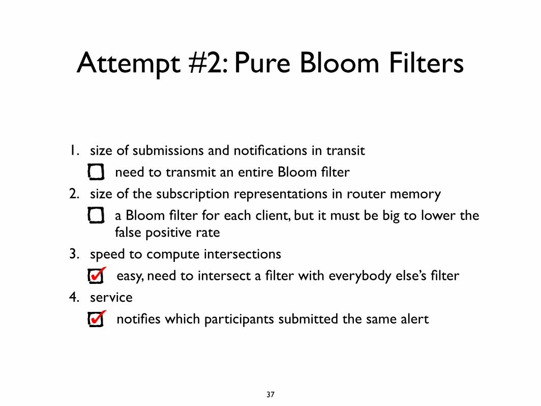
Attempt #2: Pure Bloom Filters
1. size of submissions and notifications in transit
need to transmit an entire Bloom filter
2. size of the subscription representations in router memory
a Bloom filter for each client, but it must be big to lower the false positive rate
3. speed to compute intersections
easy, need to intersect a filter with everybody else’s filter
4. service
notifies which participants submitted the same alert
37
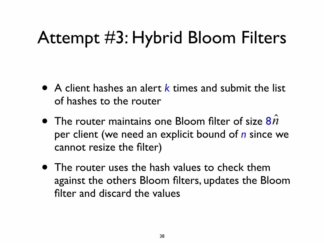
Attempt #3: Hybrid Bloom Filters
• A client hashes an alert k times and submit the list of hashes to the router
• The router maintains one Bloom filter of size 8 per client (we need an explicit bound of n since we cannot resize the filter)
• The router uses the hash values to check them against the others Bloom filters, updates the Bloom filter and discard the values
!
"#$$%&'!('!)*+'! ,(%!-.%%/! 01.,'2&!%0! &13'!m! 41,&5! '*6)!
&,%2178!n!91&,176,!+*.#'&!:1;';5!7%!+*.#'&!17!6%//%7<!#&178!
k! 41,&! $'2! 1,'/;! ! =! 41,! 17! ,)'! 01.,'2! (1..! 4'! &',! (1,)!
$2%4*41.1,>!p5!2%#8).>! ! "knm??? ## ;!!@%2!%$,1/*.!-.%%/!
01.,'2&5! p! &)%#.9! 4'! 7'*2! A;B5! *.,)%#8)! ('! 6*7! /*C'! 1,!
/#6)!&$*2&'2!*,!,)'!6%&,!%0!1762'*&'9!/'/%2>!#&*8';!!!
@%2!%#2!6*7919*,'!-.%%/!01.,'25!('!6*7!+1'(!,)'!6*&'!
,)*,!%7'!%0!%#2!41,&!6%17619'7,.>!/*,6)'&!*!41,!17!,)'!%,)'2!
01.,'2!*&!*!-'27%#..1!,21*.!(1,)!6)*76'!%0!DB'&&E!p;!!F)'!
7#/4'2! %0! /*,6)178! 41,&! (1..! ,)'7! 0%..%(! *! 417%/1*.!
91&,214#,1%75!(1,)!,)'!'G$'6,'9!7#/4'2!%0!B'&&'&!17!kn!
,21*.&! 'H#*.! ,%! knp;! ! I%/$#,'2! &1/#.*,1%7! 6%7012/&! ,)'!
*66#2*6>!%0!,)1&!*7*.>&1&;!!knp!(1..!4'!+*&,.>!82'*,'2!,)*7!
k5! *79! ,)#&! ,)'! 7#/4'2! %0! 0*.&'! $%&1,1+'&! (1..! 4'!
'7%2/%#&;! ! J+'7! 10! ('! ,2>! ,%! .%('2! knp! 4>! /*C178! p!
'G,2'/'.>!&/*..!:*79!/*C178!,)'!01.,'2!'G,2'/'.>!&$*2&'<5!
.*28'! +*.#'&! %0! n! (1..! 2*$19.>! /*C'! ,)'! &1,#*,1%7!
#7(%2C*4.';!!!
@%2!17&,*76'5!10!k!1&!K5!*79!,)#&!('!(*7,!%#2!'G$'6,'9!
7#/4'2!%0!6%..1&1%7&!,%!4'!.'&&!,)*7!K5!('!/#&,!$#,!0'('2!
,)*7!?LAA!1,'/&!17,%!*7!M!/1..1%7!41,!:?N-<!-.%%/!01.,'2!
:kOK5!nO??MP5!mOLLP5!p!A;AAAM5!knp!K;A<;!!Q%,'!,)*,!,)1&!
6%&,! 1&! %7.>! 176#22'9! 17!/'/%2>;! !R'! 6*7! 6%/$2'&&! ,)'!
01.,'2!9#2178!7',(%2C!,2*7&/1&&1%7!4>!*!.*28'!0*6,%2!#&178!
&,*79*29!6%/$2'&&1%7!,%%.&;!!Q%7',)'.'&&5!*79!'+'7!81+'7!
,)'!&$''9!%0!&1/$.>!=QS178!,)'!,(%!.*28'!-.%%/!01.,'2&!
,%8',)'25! TAAAU! 41,&! $'2! 1,'/! &,%2'9! 1&! *! )18).>!
#7*,,2*6,1+'!2*,1%;!
!
Hybrid Bloom Filter
R'! 6*7! B'&&0#..>! .'+'2*8'! ,)'! &13'! *9+*7,*8'! %0!
-.%%/! 01.,'2&! 4>! 6%/417178! ,)'/! (1,)! ,)'! &',V%0V)*&)V
+*.#'&! *$$2%*6);! ! W*2,161$*7,&! /1,! ,)'! .1&,! %0! )*&)!
+*.#'&! %0! 17,'2'&,5! 2'$2'&'7,178! 7%,'9! 17&,*76'&! %0!
&#&$161%#&! 7',(%2C! *6,1+1,>;! ! F)'! 2%#,'2! #&'&! ,)'! *6,#*.!
)*&)!+*.#'&!,%!6)'6C!*8*17&,!,)'!-.%%/!01.,'2&!%0!,)'!%,)'2!
$*2,161$*7,&!,%!0179!/*,6)'&!(1,)!2'*&%7*4.'!*66#2*6>;!!X0!
/*,6)'&! *2'! 0%#795! ,)'! 2%#,'2! &'79&! ,)'!/*,6)178!+*.#'&!
*&! *! 7%,1016*,1%7! ,%! *..! /*,6)178! $*2,161$*7,&;!!
=991,1%7*..>5!,)'!2%#,'2!6%7+'2,&!,)'!/1,,'9!&',!%0!)*&)!
+*.#'&!17,%!*!-.%%/!01.,'2!%0!&13'! nYM !41,&5!()'2'! nY !1&!,)'!
'&,1/*,'9! ,%,*.!7#/4'2!%0!+*.#'&!$'2!$*2,161$*7,!:/*C178!
*..! 01.,'2&! ,)'! &*/'! &13'5! *79! 81+178! *! 6)*76'! %0! 0*.&'!
$%&1,1+'! *2%#79! LZ<;! ! F)1&! 01.,'2! 1&! ,)'7! &,%2'9! *79!
*&&%61*,'9!(1,)! ,)'!/1,,'2;! !=0,'2!*..!%0! ,)'!/1,,'9!
)*&)! +*.#'&! )*+'! 4''7! 6)'6C'9! *8*17&,! '+'2>%7'! '.&'[&!
-.%%/! 01.,'2&5! ,)'! 2%#,'2! 6*7! ,)'7! 91&6*29! ,)'! /1,,'9!
)*&)! +*.#'! .1&,5! .'*+178! %7.>! ,)'! &6214'2[&! :/#6)!
&/*..'2<!-.%%/!01.,'2;!!!
F)#&! $#4.1&)'2&! /1,! .*28'! &',&! %0! )*&)! +*.#'&5!
()16)! *2'! #&'9! ,%! 0179! /*,6)'&5! *79! ,)'7! .'*+'! 4')179!
/#6)! &/*..'2! -.%%/! 01.,'2! D2'&19#'&E! ,)*,! *6,! *&!
&621$,1%7&;! ! N*,6)178! )*&)! +*.#'! &',&! :%$,1%7*..>!
,*88'9!(1,)!,)'!19'7,1,>!%0!,)'12!/1,,'2<!*2'!&'7,!%#,!*&!
,)'!*6,#*.!7%,1016*,1%7&;!!@%2!,)1&!9%/*175!('!*&&#/'!,)*,!
,)'!7#/4'2!%0!7%,1016*,1%7&!1&!+'2>!&/*..!17!2'.*,1%7!,%!,)'!
7#/4'2! %0! +*.#'&! /1,,'9! :'G$'21/'7,&! &)%(!
6%22'.*,1%7! 2*,'&! %0! A;A?Z! %2! .%('2<;! ! X0! ,)'! 7#/4'2! %0!
/*,6)'&! 1&!'G$'6,'9! ,%!4'! .*28'5! ,)'!/*,6)178!&',&!6%#.9!
,)'/&'.+'&! 4'! 6%7+'2,'9! ,%! -.%%/! 01.,'2&! 4'0%2'! 4'178!
&'7,!*&!7%,1016*,1%7&5!(1,)!,)'!*,,'79*7,!&$*6'!&*+178&;!!!
Q%,'! ,)*,! ,)'! )*&)! +*.#'&! #&'9! 0%2! -.%%/! 01.,'2!
8'7'2*,1%7!*2'!/#6)!.*28'2!,)*7!,)'!)*&)!+*.#'&!#&'9!4>!*!
$.*17!)*&),*4.'5!'+'7! ,)%#8)! ,)'! 2'&#.,178! 01.,'2!&,2#6,#2'!
1&! &/*..'2! ,)*7! ,)'! 6%22'&$%79178! )*&),*4.';! ! @%2! '*6)!
1,'/! '7,'2'95! -.%%/! 01.,'2&! 7''9! k! 17916'&! 17,%! *7!mV41,!
,*4.'5! *79! ,)#&! *! ,%,*.! %0!k.7m! 41,&! %0! )*&)!$'2! 1,'/;! ! X0!
mOMn5! ,)'7! k:PU.7n<! 41,&;! ! @%2! &',&! %0! L5AAA! ,%! ?LM5AAA!
1,'/&!*79!COK5!,)1&!(%2C&!%#,!,%!M\V?LA!41,&!$'2!1,'/5!%2!*!
0*6,%2! %0! PV\! 1762'*&'! %+'2! ,)'! &13'! %0! ,)'! )*&)! +*.#'&!
7''9'9!0%2!$.*17!)*&),*4.'&;!!F)1&!(%#.9!$%,'7,1*..>!4'!*!
$2%4.'/!0%2!,)'!/1&&1%7!%0!.*28'!&',&!%0!)*&)'9!+*.#'&!
17!,)'!)>4219!6*&';!
]%('+'25!('! 6*7! *+%19! ,)1&! $2%4.'/!4>!)*&)178!%#2!
*.'2,&!,%!PL!41,&!0%2!,2*7&/1&&1%75!*79!,)'7!2')*&)178!'*6)!
,%!?LAU!41,&!*0,'2!1,!*221+'&!*,!,)'!&'2+'2!:*79!,)'7!&$.1,,178!
#$!,)%&'!41,&!17,%!,)'!C!17916'&!%0!&13'!.7m!,)*,!('!7''9<5!
,)#&!/*C178!,)'!,2*7&/1&&1%7!6%&,!7%!/%2'!'G$'7&1+'!,)*7!
0%2! $.*17! )*&),*4.'&;! ! "176'! ,)'! %21817*.! *.'2,&! (1..!
,>$16*..>! 6%7,*17! .'&&! ,)*7! PL! 41,&! %0! '7,2%$>5! 7%!
170%2/*,1%7! &)%#.9! 4'! .%&,! (1,)! ,)1&! ,(%V&,*8'! )*&)178!
$2%6'&&;!
!
Optimization with Two-Stage Compare
X7! ,)'! )>4219! 6*&'! 9'&6214'9! *4%+'5!('! *&&#/'9! ,)*,!
,)'! 2%#,'2!/*17,*17&! *! &'$*2*,'! -.%%/! 01.,'2! 0%2! '*6)! %0!
,)'!C!6%..*4%2*,178!$*2,1'&5!2'$2'&'7,178!,)'!&$'61016!&',!%0!
*.'2,&! &''7! 4>! ,)*,! $*2,>;! !R)'7! *! 7'(! &',! %0! +*.#'&! 1&!
$#4.1&)'95! 1,!/#&,! 4'! 6%/$*2'9! *8*17&,! '*6)! %0! ,)'!C-1!
%,)'2!&',&;!!R'!6*7!&$''9!$2%6'&&178!4>!'7,'2178!*..!%0!,)'!
/1,,'9! +*.#'! &',&! 17,%! *! &178.'! .*28'! D/*&,'2E!-.%%/!
01.,'2!17!,)'!^%#,'2!*79!6)'6C178!,)1&!012&,;!!!
X0!('!0179!*!/*,6)!17!,)'!/*&,'2!-.%%/!01.,'25!('!/#&,!
,)'7! 6)'6C! '*6)! 1791+19#*.! 01.,'2! ,%!91&6%+'2! ,)'! &$'61016!
$*2,161$*7,&! ()%! /*,6)'9;! ! S'&$1,'! ,)1&5! ('! (1..! &)%(!
,)*,!,)1&!*$$2%*6)!6*7!%00'2!&,*7,1*.!&$*6'!'00161'761'&!
%+'2!,)'!)*&)!,*4.'!*$$2%*6)5!*79!,)'!&$''9!91&*9+*7,*8'!
6*7!4'!2'9#6'9;!
R'! 6*7! &$''9! %#2! -.%%/! 01.,'2! .%%C#$&! 4>! ,*C178!
*9+*7,*8'! %0! *21,)/',16! /%9#.%! Lm! %7! 417*2>! 7#/4'2&;!!
_#&,! *&! *! 4*&'! ?A! 7#/4'2! /%9#.%! ?Am! 1&! ,)'! .'*&,!
&1871016*7,! m! 9181,&! %0! ,)'! 7#/4'25! *! 417*2>! 7#/4'2!
/%9#.%!Lm!1&!`#&,!,)'!4%,,%/!m!41,&!%0!,)'!7#/4'25!()16)!
6*7! 4'! 'G,2*6,'9! 4>! =QS178! ,)'! 7#/4'2! (1,)! *7!
*$$2%$21*,'! 41,! /*&C! :(1<<m)–1! #&178! ,)'! IV.*78#*8'!
41,!%$'2*,%2&<;!
a',!n’!4'!,)'!$%('2!%0!L!6.%&'&,!,%!n;! !R'!62'*,'!%7'!
/*&,'2!-.%%/!01.,'2!%0!&13'!Cn’!*79!*!01.,'2!%0!&13'!n’!0%2!
'*6)!%0!,)'!C!$*2,161$*7,&;!!"13178!,)'&'!*,!M!41,&!$'2!1,'/5!
38
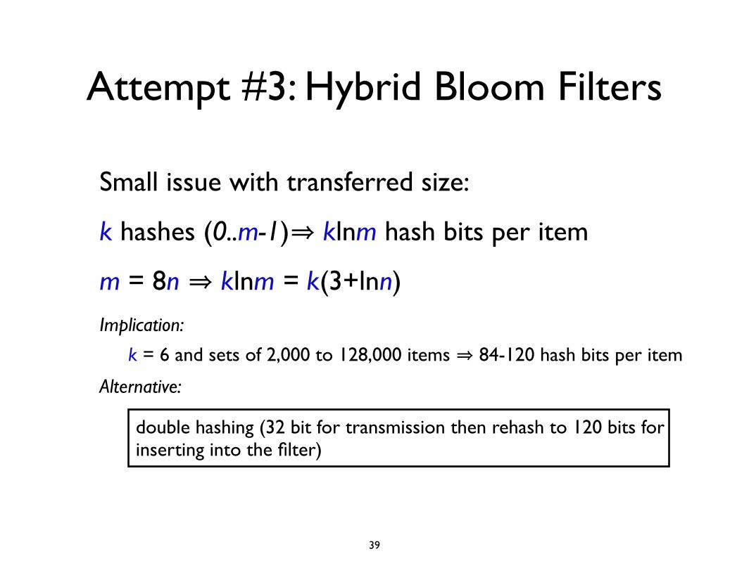
Attempt #3: Hybrid Bloom Filters
Small issue with transferred size:
k hashes (0..m-1)⇒ klnm hash bits per item
m = 8n ⇒ klnm = k(3+lnn)
Implication:
Alternative:
39
k = 6 and sets of 2,000 to 128,000 items ⇒ 84-120 hash bits per item
double hashing (32 bit for transmission then rehash to 120 bits for inserting into the filter)
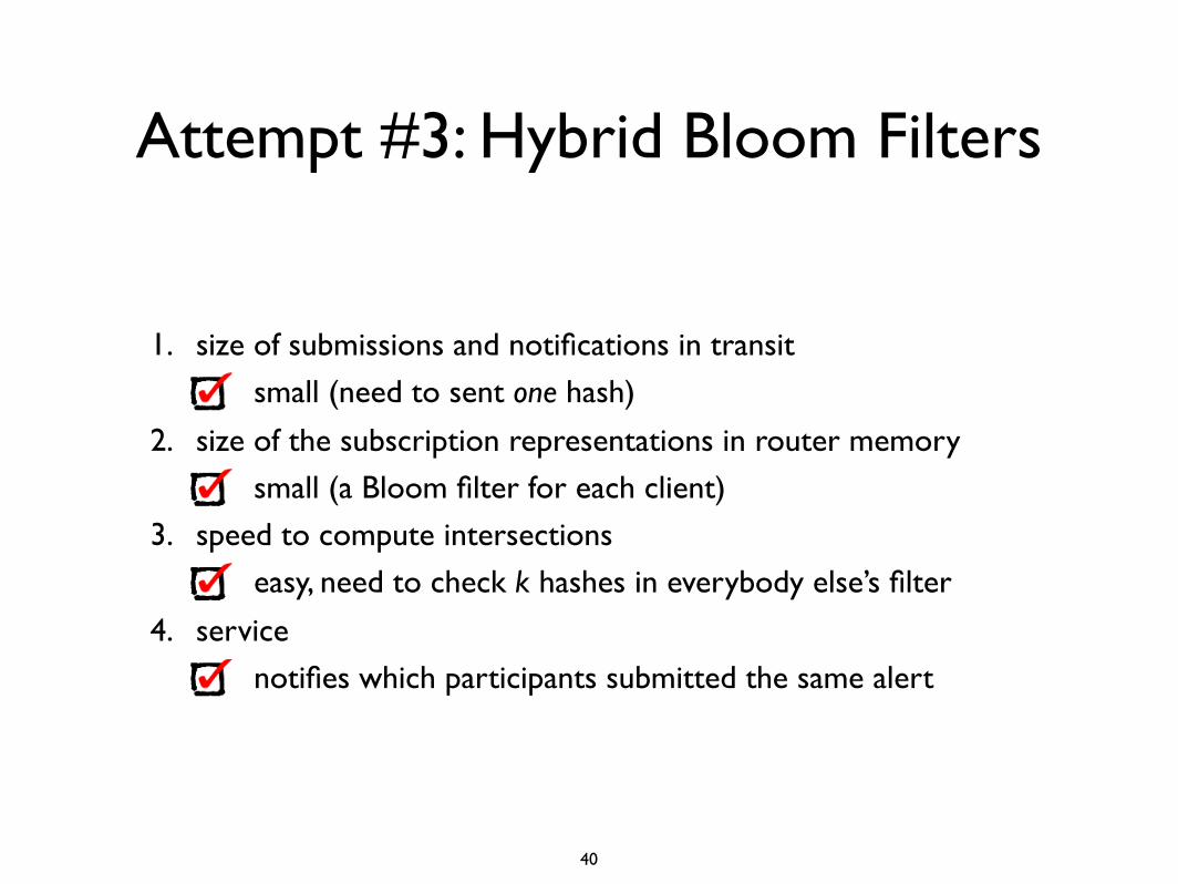
Attempt #3: Hybrid Bloom Filters
1. size of submissions and notifications in transit
small (need to sent one hash)
2. size of the subscription representations in router memory
small (a Bloom filter for each client)
3. speed to compute intersections
easy, need to check k hashes in everybody else’s filter
4. service
notifies which participants submitted the same alert
40
Mapping Internet Passive Monitors
Mapping Internet Sensors With Probe Response AttacksJohn Bethencourt, Jason Franklin, Mary Vernon
Vulnerabilities of Passive Internet Threat MonitorsYoichi Shinoda (JAIST),Ko Ikay (National Police Agency, Japan),Motomu Itoh (JPCERTC/CC)
USENIX Security 2005
41
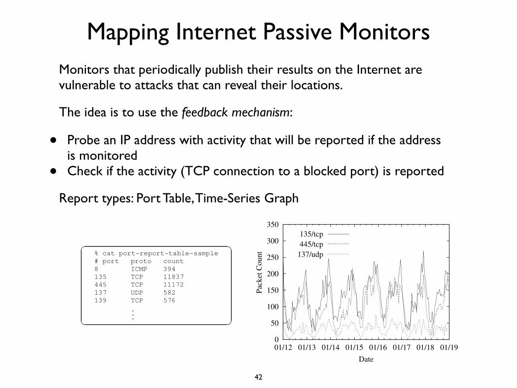
Mapping Internet Passive MonitorsMonitors that periodically publish their results on the Internet are vulnerable to attacks that can reveal their locations.
The idea is to use the feedback mechanism:
• Probe an IP address with activity that will be reported if the address is monitored
• Check if the activity (TCP connection to a blocked port) is reported
Report types: Port Table, Time-Series Graph
Sensor Mobility Sensors may be listening to fixed ad-dresses or dynamically assigned addresses, de-pending on how they are deployed. Large, tele-scope type sensors with extremely large aperturesuch as /8 are likely to be listening on fixed ad-dresses, while small aperture sensors, especiallythose hooked up to DSL providers are very likelyto be listening to dynamically changing addresses.
Sensor Intelligence Some systems deploy firewall typesensors that capture questionable packets withoutdeep inspection, while others deploy intrusion de-tection systems that are capable of classifying whatkind of attacks are being made based on deep in-spection of captured packets.
There are some sensors that respond to certainnetwork packets making them not quite “passive”to capture payloads that all-drop firewall type sen-sors cannot. [7, 8].
Sensor Data Authenticity Some systems use sensorsprepared, deployed and operated by institutions,while others rely on volunteer reports from the gen-eral public.
We see no fundamental difference between tradi-tional, so called “telescope” threat monitors and “dis-tributed sensor” threat monitors as they all listen to back-ground traffic. In this paper, we focus on detecting sen-sors of distributed threat monitors, but it is straightfor-ward to extend our discussion to large telescope moni-tors.
2.2.2 Report TypesAll reports are generated from a complete database ofcaptured events, but exhibit different properties basedon their presentation. There are essentially two types ofpresentation styles: the data can be displayed as “graph”or in “table” format.
Port Table Table type reports tend to provide accurateinformation about events captured over a range ofports. Figure 2 shows the first few lines from a hy-pothetical report table that gives packet counts forobserved port/protocol pairs.
Time-Series Graph The graph type reports resultfrom visualizing an internal database, and tend toprovide less information because they summarize!
"
#
$
% cat port-report-table-sample# port proto count8 ICMP 394135 TCP 11837445 TCP 11172137 UDP 582139 TCP 576
.
..
Figure 2: An Example of Table Type Report
events. The graphs we will be focusing on are theones that have depict explicit time-series, that is,the graph represents changes in numbers of eventscaptured over time. Table type reports also havetime-series property if they are provided periodi-cally, but graphs tend to be updated more frequentlythan tables.
Figure 3 shows an hypothetical time-series graphreport. It contains a time-series of the packets re-ceived per hour for three ports, during a week longperiod starting January 12th.
We examine other report properties in detail inSection 4.2.
0
50
100
150
200
250
300
350
01/12 01/13 01/14 01/15 01/16 01/17 01/18 01/19
Pack
et C
ount
Date
135/tcp445/tcp
137/udp
Figure 3: An Example of Time Series Graph Feedback,showing only three most captured events.
2.3 Existing Threat MonitorsIn addition to threat monitors already mentioned, thereare many similar monitors deployed around the World.For example, SWITCH [9] operate telescope type mon-itors.
Examples of distributed sensor monitors are the mon-itor run by the National Police Agency of Japan [10],ISDAS (Internet Scan Data Acquisition System) run byJPCERT/CC [11] and WCLSCAN [12] which is uniquein that it uses sophisticated statistical algorithms to esti-mate background activity trends. The IPA (Information-Technology Promotion Agency, Japan) is also known tooperate two versions of undocumented threat monitorcalled TALOT (Trends, Access, Logging, Observation,Tool) and TALOT2.
University of Michigan is operating the Internet Mo-tion Sensor, with multiple differently sized wide aper-ture sensors [13, 14]. Telecom-ISAC Japan is alsoknown to operate an undocumented and unnamed threatmonitor that also combines several different sensorplacement strategies. PlanetLab[15] has also announced
42
Port table attack
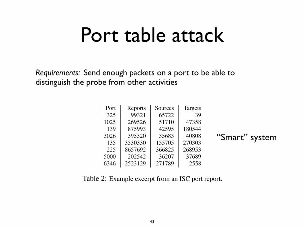
Requirements: Send enough packets on a port to be able to distinguish the probe from other activities
Port Reports Sources Targets325 99321 65722 39
1025 269526 51710 47358139 875993 42595 180544
3026 395320 35683 40808135 3530330 155705 270303225 8657692 366825 268953
5000 202542 36207 376896346 2523129 271789 2558
Table 2: Example excerpt from an ISC port report.
is not possible to carry out such attacks. Little to no at-tention has been given to the problem of discovering thelocation of the sensors. We provide techniques that ac-complish this. In addition, little attention has been givento the fact that the identity of the organizations and thespecific addresses they monitor must remain secret to en-sure the integrity of the statistics produced by the anal-ysis center, particularly if the statistics are meant to beemployed in stemming malicious behavior. By demon-strating that it is possible to foil the current methods formaintaining the secrecy of the sensor locations, we showthe importance of this issue.
For example, Pang and Paxson [32] consider the pos-sibility of “indirect exposure” allowing attackers to dis-cover the values of anonymized data fields by consid-ering other parts of the available information. They donot, however, consider how or whether one might beable to map the locations of Internet sensors, a prereq-uisite to interacting with them. Similarly, Xu et al. [28]describe a prefix-preserving permutation based methodfor anonymizing IP addresses that is provably as secureas the TCPdpriv scheme [27] and consider the extent towhich additional address mappings may be discovered ifsome are already known. They also mention active at-tacks in passing and point out that defense against theseattacks is tricky. We develop in depth an active map-ping attack that is effective even on reports that subjectIP addresses to prefix-preserving permutations and fur-ther discuss countermeasures.
3 Background: the Internet Storm Center3.1 OverviewThe Internet Storm Center of the SANS Institute is one ofthe most important existing examples of systems whichcollect data from Internet sensors and publish public re-ports. Furthermore, it is a challenging network to map,as will be shown in Section 5.5, due to its large numberof sensors with non-contiguous IP addresses. Thus, inorder to demonstrate the possibility of mapping sensorswith probe response attacks in general, we describe andevaluate the algorithm initially using the ISC and thengeneralize the algorithm and simulation results to othersensor networks. In this way, the ISC serves as a casestudy in the feasibility of mapping sensor locations.
The ISC collects firewall and IDS logs from approxi-
mately 2,000 organizations, ranging from individuals touniversities and corporations [33]. This collection takesplace through the ISC’s DShield project [34]. The ISCanalyzes and aggregates this information and automati-cally publishes several types of reports which can be re-trieved from the ISC website. These reports are useful fordetecting new worms and blacklisting hosts controlled bymalicious users, among other things. Currently, the logssubmitted through the DShield project are almost en-tirely packet filter logs listing failed connection attempts.They are normally submitted to the ISC database auto-matically by client programs running on the participatinghosts, typically once per hour. The logs submitted are ofthe form depicted in Table 1. These logs are used to pro-duce the reports published by the ISC, including the topten destination ports and source IP addresses in the pastday, a “port report” for each destination port, a “subnetreport,” autonomous system reports, and country reports.
3.2 Port ReportsIn general, many types of information collected by In-ternet sensors and published in reports may be used toconduct probe response attacks, as will be discussed inSection 6. For our case study using the ISC, we will pri-marily concern ourselves with the ISC’s port reports, asthese are representative of the type of statistics that otherInternet sensor networks may provide and are general innature. A fictional excerpt of a port report is given inTable 2. A full listing all of the 216 possible destina-tion ports that had any activity in a particular day maybe obtained from the ISC website. For each port, thereport gives three statistics, the number of (unfortunatelynamed) “reports,” the number of sources, and the numberof targets. The number of sources is the number of dis-tinct source IP addresses appearing among the log entrieswith the given destination port; similarly, the number oftargets is the number of distinct destination IP addresses.The number of “reports” is the total number of log en-tries with that destination port (generally, one for eachpacket). Although the port reports are presented by dayand numbers in the port report reflect the totals for thatday, the port reports are updated more frequently thandaily. One may gain the effect of receiving a port re-port for a more fine-grained time interval by periodicallyrequesting the port report for the current day and sub-tracting off the values last seen in its fields.
4 Example AttackWe now present a detailed algorithm which uses astraightforward divide and conquer strategy along withsome less obvious practical improvements to map thesensor locations using information found in the ISC portreports. In Section 6 we outline how the algorithm couldbe applied to map the sensors in other networks (includ-ing Symantec DeepSight and myNetWatchman) usinginformation in those sensor network reports.
14th USENIX Security SymposiumUSENIX Association 195
43
“Smart” system
Port table attack
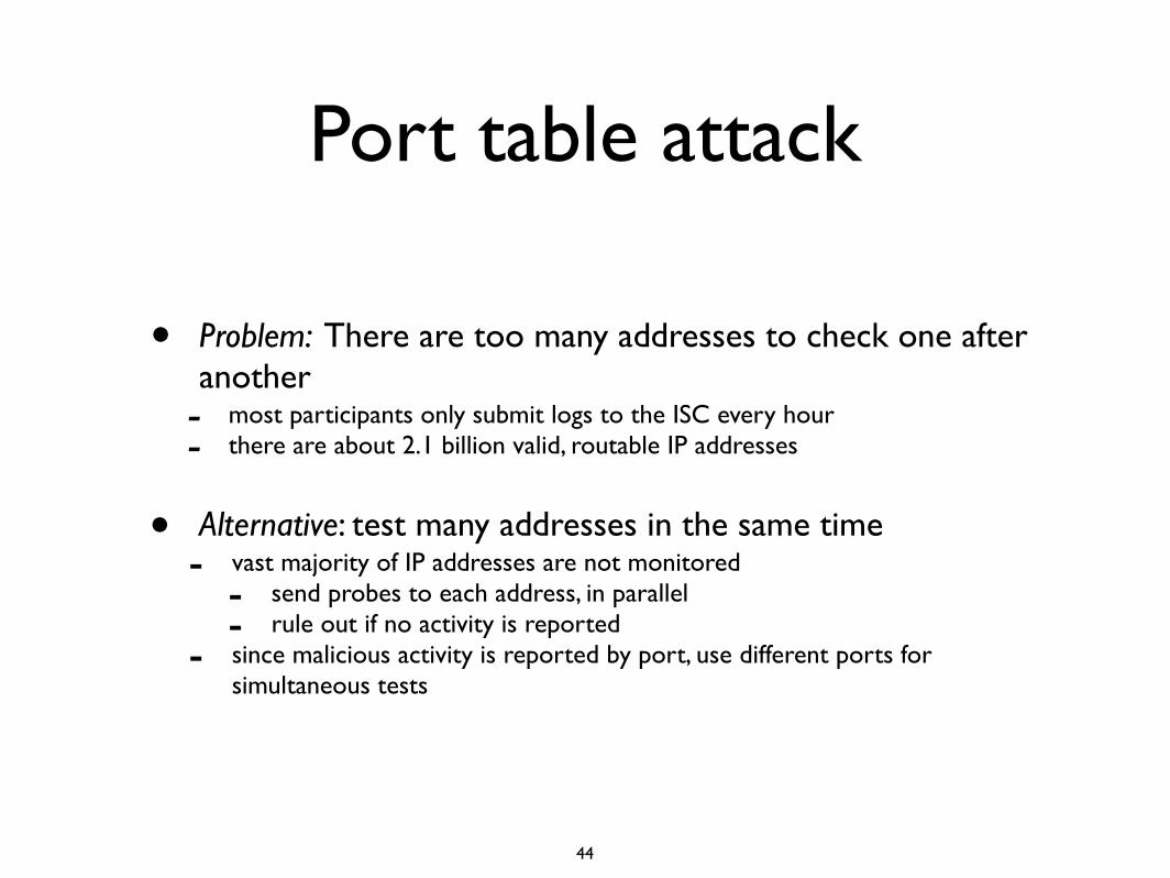
• Problem: There are too many addresses to check one after another- most participants only submit logs to the ISC every hour- there are about 2.1 billion valid, routable IP addresses
• Alternative: test many addresses in the same time- vast majority of IP addresses are not monitored
- send probes to each address, in parallel- rule out if no activity is reported
- since malicious activity is reported by port, use different ports for simultaneous tests
44
Basic Probe Response Attack
14th USENIX Security Symposium
... ...
......
S3
...
SnS2
...
S1
1
packetson port p 2
packetson port p 3
packetson port p n
packetson port p
IP address space
Figure 1: The first stage of the attack.
4.1 Introduction to the AttackThe core idea of the attack is to probe an IP address withactivity that will be reported to the ISC if the addressesare among those monitored, then check the reports pub-lished by the network to see if the activity is reported.If the activity is reported, the host probed is submittinglogs to the ISC. Since the majority of the reports indi-cate an attempt to make a TCP connection to a blockedport (which is assumed to be part of a search for a vul-nerable service), a single TCP packet will be detectedas malicious activity by the sensor.1 To distinguish ourprobe from other activity on that port, we need to sendenough packets to significantly increase the activity re-ported. As it turns out, a number of ports normally havelittle activity, so this is not burdensome. This issue willbe further discussed in Section 4.3. This probing proce-dure is then used for every possible IP address. It is quitepossible to send several TCP/IP packets to every address;the practical issues relating to such a task are consideredin Section 5.
The simplest way to find all hosts submitting logs tothe ISC is then to send packets to the first IP address,check the reports to determine if that address is moni-tored, send packets to the second IP address, check thereports again, and so on. However, some time must beallowed between sending the packets and checking thereports. Participants in the ISC network typically submitlogs every hour, and additional time should be allowedin case some participants take a little longer, perhaps fora total wait of two hours. Obviously, at this rate it willtake far too long to check every IP address one by one.
In order for a sensor probing attack to be feasible,we need to test many addresses at the same time. Twoobservations will help us accomplish this. First, thevast majority of IP addresses either do not correspondto any host, or correspond to one that is not submittinglogs. With relatively few monitored addresses, there willnecessarily be large gaps of unmonitored address space.Hence, we may be able to rule out large numbers of ad-dresses at a time by sending packets to each, then check-ing if any activity is reported at all. If no activity isreported, none of the addresses are monitored. Send-ing packets to blocks of addresses numerically adjacent
is likely to be especially effective, since monitored ad-dresses are likely to be clustered to some extent, leav-ing gaps of addresses that may be ruled out. Second,since malicious activity is reported by port, we can usedifferent ports to conduct a number of tests simultane-ously. These considerations led the authors to the methoddescribed in the following section. It is worth notingthat the problem solved by this algorithm is very similarto the problems of group blood testing [35]. However,much of theoretical results from this area focus on op-timizing the solutions in a different way than we wouldlike to and thus are not directly applicable to this prob-lem.
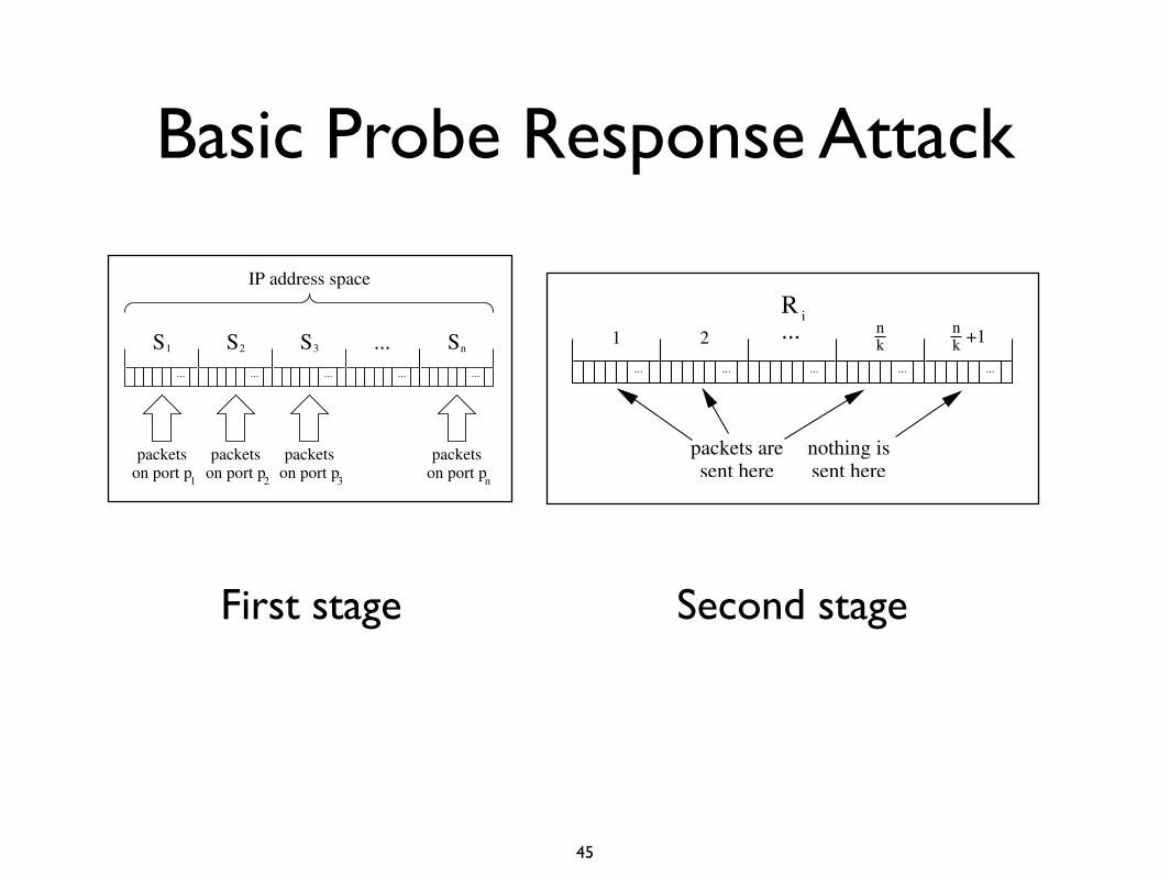
4.2 Basic Probe Response AlgorithmFirst Stage
We begin with 0, 1, 2, . . .232 − 1 as our (ordered) list ofIP addresses to check. As a preprocessing step, we fil-ter out all invalid, unroutable, or “bogon” addresses [36].Approximately 2.1 billion addresses remain in the list.Suppose n ports p1, p2, . . . pn can be used in conductingprobes. To simplify the description of the basic algo-rithm, we assume in this section that these ports do nothave any other attack activity; we relax this restrictionin Section 4.3. In the first stage of the attack, we di-vide the list of addresses into n intervals, S1, S2, . . . Sn.For i ∈ {1, . . . n}, we send a SYN packet2 on port pi toeach address in Si, as depicted in Figure 1. We then waittwo hours and retrieve a port report for each of the ports.Note that we now know the number of monitored ad-dresses in each of the intervals, since the reports tell notonly whether activity occurred, but also give the numberof targets. All intervals lacking any activity may be dis-carded; the remaining intervals are passed to the secondstage of the attack along with the number of monitoredaddresses in each.
Second StageThe second stage of the attack repeats until the attack iscomplete. In each iteration, we take the k intervals thatcurrently remain, call them R1, . . . Rk, and distribute ourn ports among them, assigning n
k to each.3 Then for eachi ∈ {1, . . . k}, we do the following. Divide Ri into n
k +1subintervals, as shown in Figure 2. We send a packeton the first port assigned to this interval to each addressin the first subinterval, a packet on the second port toeach address in the second subinterval, and so on, finallysending a packet on the last port to each address in thenk th subinterval, which is the next to last. We do not sendanything to the addresses in the last subinterval. We willinstead deduce the number of monitored addresses in thatsubinterval from the number of monitored addresses inthe other subintervals. After this process is completedfor each of the subintervals of each of the remaining in-tervals, we wait two hours and retrieve a report. Now weare given the number of monitored addresses in each of
USENIX Association196
packets aresent here
nothing issent here
...... ...... ...
+1nk1 2
R i
kn...
Figure 2: Subdividing an interval Ri within thesecond stage of the attack.
the subintervals except the last in each interval. We thendetermine the number in the last subinterval of each in-terval by subtracting the number found in the other subin-tervals from the total known to be in that interval. At thispoint, empty subintervals may again be discarded. Ad-ditionally, subintervals with a number of monitored ad-dresses equal to the number of address in the subintervalmay be discarded after adding their addresses to a list ofmonitored addresses found so far. The remaining subin-tervals, which contain both monitored addresses and un-monitored addresses, may now be considered our newset of remaining intervals R′
1, . . .R′k′ , and we repeat the
procedure.By continuing to subdivide intervals until each is bro-
ken into pieces full of monitored addresses or withoutany monitored addresses, we eventually check every IPaddress and produce a list of all that are monitored. Thisprocess may be visualized as in Figure 3, which gives anexample of the algorithm being applied to a small num-ber of addresses. The first row of boxes in the figurerepresent the initial list of IP addresses to be checked,with monitored addresses shaded. Six ports are used toprobe these addresses, giving the numbers of monitoredaddresses above the row. Three intervals are ruled out asbeing empty, and the other three are passed to the secondstage of the algorithm. The six ports are used in the firstiteration of the second stage to eliminate three subregions(of two addresses each), and mark one subregion as filledwith monitored addresses. The second iteration of thesecond stage of the algorithm terminates, having markedall addresses as either monitored or unmonitored. Onecaveat of the algorithm that did not arise in this exampleis that the number of remaining intervals at some stagemay exceed n, the number of available ports. In this caseit is not possible to divide all those intervals into subinter-vals in one time period, since at least one port is neededto probe each interval. When this cases arises, we simplyselect n of the subintervals to probe, and save the othersubintervals for the next iteration.
4.3 Dealing With NoiseWe now turn to a practical problem that must be ad-dressed if the attack is to function correctly. The problemis that sources other than the attacker may also be send-ing packets to monitored addresses with the same desti-
nation ports that the algorithm is using, inflating the num-ber of targets reported. This can cause the algorithmto produce both false positives and ports reports
561 ≤ 519, 364 ≤ 1041, 357 ≤ 1551, 959 ≤ 2056, 305 ≤ 25
Table 3: Ports withlittle activity.
false negatives. This backgroundactivity may be considered noisethat obscures the signal the attackerneeds to read from the port reports.For a large number of ports, how-ever, this noise is typically quitelow, as shown by Table 3. Eachrow in the table gives the approx-imate number of ports that typically have less than thegiven number of reports. The numbers were producedby recording which ports had less than the given num-ber of reports every day over a period of ten consecutivedays.
A simple technique allows the algorithm to tolerate acertain amount of noise at the expense of sending morepackets. If there are normally, say, less than five reportsfor a given port p, we may use port p to perform probesin our algorithm by sending five packets whenever wewould have otherwise sent one. Then when reviewingthe published port report, we simply divide the numberof reports by five and round down to the nearest integerto obtain the actual number of submitting hosts we hit.We subsequently refer to this practice as using a “reportnoise cancellation factor” of five. Thus by sending fivetimes as many packets, we may ensure that the algorithmwill function correctly if the noise on that port is less thanfive reports. Similarly, by using a report noise cancella-tion factor of ten, we may ensure the algorithm operatescorrectly when the noise is less than ten reports. By ex-amining past port reports, we may determine the least ac-tive ports and the number of packets necessary to obtainaccurate results when using them to perform probes.
4.4 ImprovementsFalse Positives and NegativesThe attack may potentially be sped up by allowing someerrors to occur. If it is acceptable to the attacker to merelyfind some superset of (i.e., a set containing) the set ofhosts submitting their logs to the ISC, they may simplyalter the termination conditions in the algorithm. Ratherthan continuing to subdivide intervals until they are de-termined to consist entirely of either monitored or un-monitored addresses, the attacker may mark all addressesin an interval as monitored and discontinue work on theinterval when it is determined to consist of at least, say,10 percent monitored addresses. In this way, when thealgorithm completes, at most 90 percent of addressesdetermined to be monitored are false positives. Eventhough that is a large amount of error, the vast majority ofthe addresses on the Internet would remain available forthe attacker to attempt to compromise, free from the fearof being detected by the ISC. Alternatively, if the attackeris willing to accept some false negatives (i.e., find a sub-
14th USENIX Security SymposiumUSENIX Association 197
First stage Second stage
45
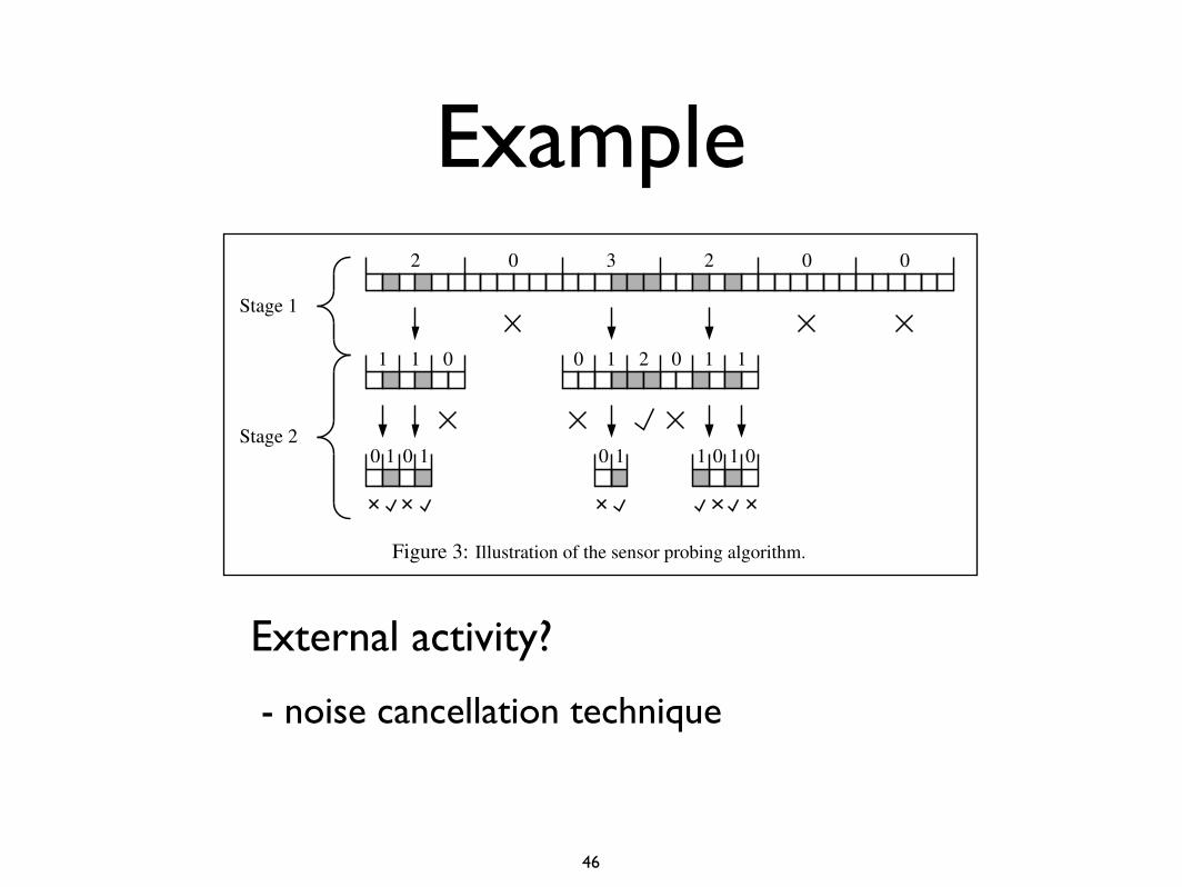
Example
14th USENIX Security Symposium
1 1 1 1 0000 01
0 0 011 1 12 1
2 0 3 2 0 0
Stage 1
Stage 2
Figure 3: Illustration of the sensor probing algorithm.
set of the hosts participating in the network), they maydiscard an interval if the fraction of the addresses that aremonitored within it is less than a certain threshold, againspeeding up the attack. In Section 5 we provide quantita-tive results on the speedup provided by these techniquesin the case of mapping the ISC.
Using Multiple Source AddressesSpeed improvements may also be obtained by taking ad-vantage of the sources field of the port reports. By spoof-ing source IP addresses while sending out probes, an at-tacker may encode additional information discernible inthis field. If in the course of probing an interval of ad-dresses with a single port, the attacker sends multiplepackets to each address from various numbers of sourceIP addresses and takes note of the number of sources re-ported, they may learn something about the distributionof monitored addresses within the interval in addition tothe number of monitored addresses. The following is amethod for accomplishing this.Multiple Source Technique Before probing an intervalof addresses on some port, we further divide the intervalinto some number of pieces k, hereafter referred to asthe “multiple source factor.” To the addresses in the firstpiece, we send packets from a single source. To each ofthe addresses in the second piece, we send packets fromtwo sources. For the third piece, we send packets fromfour source addresses to each address. In general, wesend packets from 2i−1 source addresses to each addressin the ith piece. Note that we already are sending multi-ple packets to each address in order to deal with the noisedescribed in Section 4.3. If 2k−1 is less than or equalto the report noise cancellation factor, then we can em-ploy this technique without sending any more packets;otherwise, more bandwidth is required to send all 2k−1
packets to each address.When the port report is received, we may determine
whether any of the pieces lacked monitored addresses byconsidering the number of sources reported. For exam-ple, suppose k = 3 (i.e., we divide our interval into threepieces) and five sources are reported. Then we know thatthere are monitored addresses in the first and third in-
tervals, and that there are no monitored addresses in thesecond interval. This additional information increasesthe efficiency of the probing algorithm by often reducingthe size of the intervals that need to be considered in thenext iteration, at the expense of potentially increasing thebandwidth usage. Of course, this technique is only use-ful to a limited degree, due to the exponential increasein the number of packets necessary to use it more exten-sively. Depending on the level of noise on the port, usinga multiple source factor of two or three achieves an im-provement in probing efficiency with little to no increasein the bandwidth requirements.
Noise In order for this technique to perform accurately,we must deal with noise appearing in the sources field ofthe port reports in addition to the reports field. If evena single source address other than those spoofed by theattacker is counted in the reported number of sources,the attacker will have a completely inaccurate picture ofwhich pieces are empty. This problem may be solvedin a manner similar to the method for tolerating noise inthe number of reports. Rather than sending sets of pack-ets with 1, 2, 4, . . . and 2k−1 different source addressesto the k pieces, we may use 1m, 2m, 4m, . . . and 2k−1msources, where m is a positive integer hereafter referredto as the “source noise cancellation factor.” Then thereported number of sources may be divided by m androunded down, ensuring accurate results if the noise inthe number of sources was less than m. For example,if a particular port normally has less than three sourcesreported (when the attacker is not carrying out their at-tack) and the attacker is dividing each interval into fourpieces, they may send sets of packets with 3, 6, 12, and24 sources. If seventeen sources are then reported, theydivide by three and round down to obtain five, the sumof one and four. The attacker may then conclude that thesecond and fourth intervals have no monitored addresses,and that the first and third intervals do have monitoredaddresses.
Egress Filtering There is another practical concern re-lating to this technique, and that is egress filtering ofIP packets with spoofed sources. The careful attacker
USENIX Association198
External activity?
- noise cancellation technique
46
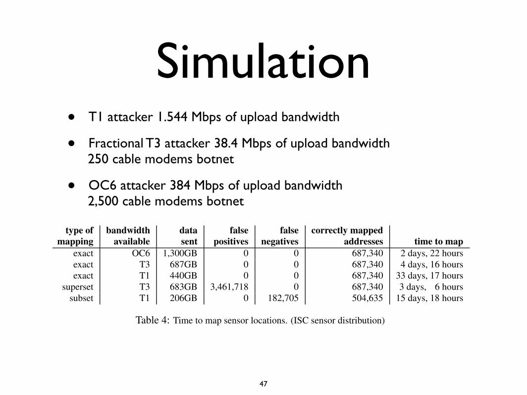
Simulation• T1 attacker 1.544 Mbps of upload bandwidth
• Fractional T3 attacker 38.4 Mbps of upload bandwidth 250 cable modems botnet
• OC6 attacker 384 Mbps of upload bandwidth 2,500 cable modems botnet
type of bandwidth data false false correctly mappedmapping available sent positives negatives addresses time to map
exact OC6 1,300GB 0 0 687,340 2 days, 22 hoursexact T3 687GB 0 0 687,340 4 days, 16 hoursexact T1 440GB 0 0 687,340 33 days, 17 hours
superset T3 683GB 3,461,718 0 687,340 3 days, 6 hourssubset T1 206GB 0 182,705 504,635 15 days, 18 hours
Table 4: Time to map sensor locations. (ISC sensor distribution)
5.4 Finding a SubsetHaving examined the cases of finding an exact set andfinding a superset, we now examine a situation where anattacker may be interested in finding a subset of the mon-itored addresses. While an attacker with a T3 or OC6may attempt to find the exact set of monitored addresses,an impatient attacker or an attacker with less resources,such as the T1 attacker, may be content with finding asubset of the monitored addresses in a reduced amountof time. By allowing false negatives, an attacker may re-duce the time and bandwidth necessary to undertake theattack, but still discover a large number of monitored IPaddresses. An attacker who is interested in flooding themonitored addresses with spurious activity rather thanavoiding them may be especially interested in allowingfalse negatives. In addition to saving time, an attackerfinding a subset may potentially avoid detection of theirattack by sending significantly fewer probes overall.
Since the difference between the time required to findthe exact set of monitored addresses and the time re-quired to find a subset of monitored addresses is less pro-nounced at high bandwidths, we only detail the results offinding a subset with the T1 adversary. Once again weuse the same parameters that were used when the T1 ad-versary found the exact set of monitored addresses, ex-cept this time we set the maximum false negative rate(i.e., the number of possible false negatives over the totalnumber of IP addresses). With a report noise cancella-tion factor of two, a single source address, and a max-imum false negative rate of .001, we are able to reducethe runtime of our attack from 33 days and 17 hours to15 days and 18 hours. In addition, we reduce the numberof probes sent from around 9.5 billion to 4.4 billion, areduction of over 50 percent. However, these reductionscome at the cost of missing 26 percent of the sensors.The progress of this scenario is depicted in Figure 6.
5.5 General Sets of Monitored AddressesThe preceding scenarios (summarized in Table 4)demonstrate that a probe response attack is practical formapping the IP addresses monitored by the ISC. Theydo not, however, reveal how dependent the running timeof the attack is on this particular set of addresses. Akey factor that determines the difficulty of mapping theaddresses of a sensor network is the extent to whichthe sensors are clustered together in the space of IP ad-
dresses. As mentioned in Section 4.1, the more the ad-dresses are clustered together, the more quickly they maybe mapped. This fact is easily seen in Figure 3.
To determine how well the algorithm works moregenerally against various possible sets of sensor IP ad-dresses, we generated random sets of IP addresses basedon a model of the clustering. More specifically, the sizesof “clusters,” or sets of sequential sensor addresses, weredrawn from a Pareto distribution,5 and the sizes of thegaps in address space between them were drawn from anexponential distribution. With the parameters of the twodistributions set to fit the actual addresses of the ISC,the times to map various random sets of IP addressesare similar to the times reported in Table 4. By vary-ing the parameters of the distributions, sets of IP ad-dresses with various average cluster sizes were producedwhile holding the total number of sensors roughly con-stant at 680,000, the approximate number in the ISCset. For average cluster sizes of 10 or more, the at-tack typically takes just over two days to complete underthe T3 attacker model previously described (comparedto the 4 days, 16 hours to complete the attack for theactual ISC). For smaller average cluster sizes, the run-ning time increases. Below the average cluster size ofthe ISC (∼ 1.9), typical running times increase rapidly,with about eight days (about twice the time to map theISC sensors) at average clusters size of about 1.6. Notethat smaller sensor networks are faster to map; the ISCnetwork is among the most challenging networks to mapdue to its large number of sensors with widely scatteredIP addresses.
As an extreme case, a number of simulations were alsorun on sets of IP addresses that possessed no special clus-tering, again using the T3 attacker model. Specifically,the sets were produced by picking one IP address afteranother, always picking each of the remaining ones withequal probability. This can be considered a worst casescenario, since any real life sensor network is likely todisplay some degree of clustering in its set of addresses.The attack remained quite feasible in this case, takingbetween two to three times as long as in the ISC casewhen working on a set of addresses of the same size.This scenario was tested for sets of IP addresses of vari-ous sizes. The running time ranged linearly from about 3days to map 100,000 addresses to about 21 days to map2,000,000.
14th USENIX Security SymposiumUSENIX Association 203
47
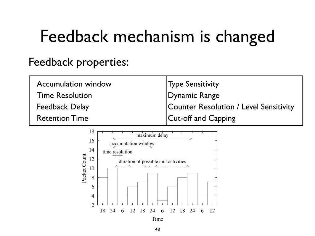
Feedback mechanism is changedFeedback properties:
Accumulation windowTime ResolutionFeedback DelayRetention Time
Type SensitivityDynamic RangeCounter Resolution / Level SensitivityCut-off and Capping
The accumulation window property affects themarking process in several different ways;
1. An attempt to introduce changes must happenwithin the accumulation window period. Inother words, the accumulation window deter-mines the maximum duration of a unit mark-ing activity.
2. The smaller the accumulation window themore address blocks can be marked in a giventime frame.
3. A smaller accumulation window requires lessmarkers to introduce changes.
Time Resolution Time resolution is the minimum unitof time that can be observed in a feedback. Thetime resolution provides a guide line for determin-ing the duration of a single marking activity. Thatis, a single marking activity should be designed tofit loosely into multiples of the time resolution forthe target system. We can not be completely ac-curate as we need to be able to absorb clock skewbetween target and marking systems.
Feedback Delay Delay is the time between a captureevent and next feedback update. For example, afeedback that is updated hourly has a maximum de-lay of one hour, while another feedback that is up-dated daily has a maximum delay of one day. Thedelay determines the minimum duration betweendifferent marking phases that is necessary to avoiddependency between them.
Most feedbacks have identical time resolution,accumulation window and delay property, but notalways. For example, there is a system which pro-vides a weekly batch of 7 daily reports, in whichcase the accumulation window is one day while themaximum delay is 7 days.
Retention Time The retention time of a feedback is themaximum duration that a event is held in the feed-back. For a graph, the width of the graph is the re-tention time for the feedback. All events older thanthe graph’s retention time are pushed out to the left.
Figure 6 illustrates the relationship between dif-ferent timing properties using a hypothetical feed-back that updates every 2 days, and provides accu-mulated packet counts for a particular day every 6hours. As shown in this figure, this feedback has atime resolution of 6 hours, a accumulation windowof 1 day, a maximum feedback delay of 2 days. Inaddition, the retention time for this graph is 3 days.The duration of some possible marking activitiesare also shown in this figure. Note that a markingactivity can span multiple resolution units, but can-not span two accumulation windows.
2
4
6
8
10
12
14
16
18
126241812624181262418
Pack
et C
ount
Time
time resolution
accumulation window
maximum delay
duration of possible unit activities
Figure 6: Timing Properties of A Hypothetical Feedback
4.2.2 Other Feedback PropertiesIn addition to the timing related properties, there is agroup of properties that mainly rule how capture eventsare presented in feedbacks. These properties also playan important role when designing marking activity.
Type Sensitivity Type sensitivity refers to the sensitiv-ity of a feedback to certain types of packets. If afeedback shows significant changes in its responseto an appropriate amount of packets of the sametype, then the feedback is sensitive to that type.
Dynamic Range The dynamic range of a feedback,which is the difference between smallest and largestnumbers in the feedback, presents another impor-tant factor in a marking design, in conjunction withthe level sensitivity property described next.
Counter Resolution / Level Sensitivity The counterresolution of a feedback is the minimal number ofpackets required to make an identifiable change inthe feedback. For example, a feedback table thatincludes information for a single event has a reso-lution of 1 packet, while the feedback in a graphthat is 100 dots high with a maximum scale (dy-namic range) of 1,000 packets has a resolution of10 packets.
We use the term “sensitivity” also to describe the“level of sensitivity”. In the above example, theformer feedback is more sensitive than the latterfeedback. Some systems use logarithmic scale fortheir feedbacks, and as a result, they are sensitive tosmall spikes even if the dynamic range of the feed-back is very large.
The unit of measurement also vary from systemto system, and affects the level sensitivity of thefeedback. Some use accumulated packet countsdirectly, in which case the sensitivity can be cal-culated easily. Others use mathematically derivedvalues such as average packet counts per sensorand packet counts per 100 sensors. In the latter
48

Possible Marking Strategies
• Advanced-Encoded-Port Marking
• Time Series Marking
• Uniform Intensity Marking
• Radix-Intensity Marking
• Radix-Port Marking
• Delayed Development Marking
49
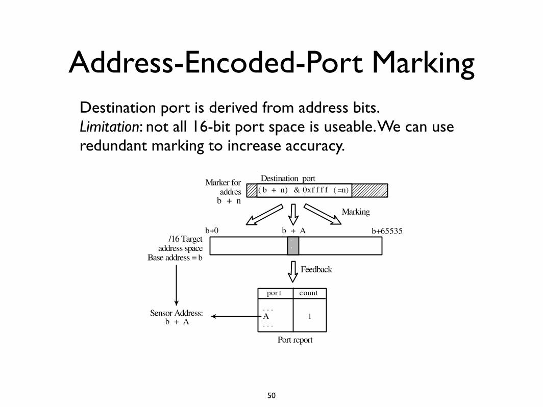
Address-Encoded-Port MarkingDestination port is derived from address bits.Limitation: not all 16-bit port space is useable. We can use redundant marking to increase accuracy.
case, number of sensors in the monitor must beknown to calculate the sensitivity. This figure maybe obtained from the background information forthe monitor, or may be estimated by comparing thefeedback with feedbacks from other monitors thatuse plain packet counts.
Cut-off and Capping Some systems drop events thatare considered non-significant. Some systems dropevents that are too significant, so events with lesssignificance are more visible. A common case ofcut-off is a feedback in the form of “Top-N” events.In this type of feedback, the top N event groups areselected, usually based on their accumulated eventcount over a predetermined period of time such asan hour, a day or a week. A feedback with the top-N property is usually very hard to exploit, becauseit often requires a large number of events to makesignificant changes such as visible spikes or an in-troduction of a new event group. However, thereis a chance of exploiting such feedback, when thefeedback exhibits certain properties, such as fre-quently changing members with low event counts,or if there is a event group with a period of inac-tivity. An introduction of a new event group is alsopossible, by “pre-charge” activity that is intendedto accumulate event counts.
4.3 Marking AlgorithmsAn algorithm used for a particular marking is often de-pends on the feedback properties. It is sometimes neces-sary to modify or combine basic marking algorithms toexploit a particular feedback, or to derive more efficientmarking algorithm. In the following, we present someexamples of possible marking algorithms.
4.3.1 Address-Encoded-Port MarkingA system providing a table of port activities may be-come a target of an address-encoded-port marking. Inthis method, an address is marked with a marker thathas its destination port number derived from encodingpart of the address bits. After the marking, port numberswhich were successfully marked are recovered from thefeedback, which are in turn combined with other addressbits to derive refined addresses.
Consider the case in Figure 7. In this example, wemark a /16 address block with base address b that is host-ing a sensor at b + A. The destination port of the markerfor address b + n is set to the 16 lower bits of the ad-dress b + n (which is equivalent to n). For the sensoraddress b + A, a marker with destination port set to A issent, which in turn appear as captured event on port A inthe port activity report. This feedback is combined withthe base address b to form the complete address of thesensor, which is b + A.
/16 Targetaddress space
Base address = b
b+0 b+65535b + A
Marker foraddres
b + n( b + n) & 0xf f f f ( =n)Destination port
Marking
Feedback
por t count
. . . A 1 . . .
Port report
Sensor Address:b + A
Figure 7: An Address-Encoded-Port Marking Example
Although the address-encoded-port marking can onlybe deployed against table type feedbacks, it is consid-ered extremely efficent, because it can deliver multiplecomplete or partial addresses from a single marking ac-tivity.
However, not all of the 16-bit port space is availablein practice; there are ports which are frequently foundin real background activity. Some of these ports, espe-cially those that are used by vulnerable, usually receivea large number of events. Other ports may also receivesome background traffic due to back scatter and stray orwandering packets.
To increase the accuracy of our method even in thepresence of background traffic for some ports, it is pos-sible to determine the usable port space in advance. Thiscan be achieved by looking at previous port-reports fromthe target system. The accuracy of this method canalso be improved by incorporating redundant markingin which multiple makers of the same type are sent tothe same address to mask the existence of busy ports.
Redundant marking also helps in dealing with packetlosses. For example, we can mark a particular addresswith four different markers, each using a destination portnumber that is encoded with 2-bits of redundancy iden-tifier and 14-bits of address information. In this case, weexamine the feedback for occurrences of these encodedports.
4.3.2 Time Series Marking
Time series marking can be used when the feedback is inthe form of a time series property. It is used in conjunc-tion with other marking algorithms such as the uniformintensity marking described next. In time series mark-ing, each sub-block is marked within the time resolutionwindow of the feedback so that results from marking canbe reverse back to the corresponding sub-block.
50
Time Series Marking
• Used in conjunction with other marking mechanisms.
• Each sub-block are marked within time resolution window to allow recovering the sub-block from the feedback.
51

Uniform Intensity Marking
Addresses are marked with the same intensity.
Mark one sub-block per time unit, marking all addresses from it with a single marker.
4.3.3 Uniform Intensity MarkingIn uniform-intensity marking, all addresses are markedwith the same intensity. For example, let’s assume thatwe are marking a /16 address block that is known to con-tain several sensors. We divide the original block into16 smaller /20 sub-blocks. Then we mark each of thesesub-blocks using time-series marking, one sub-block pertime unit, marking each address with a single marker.
0 1 2 3 4 5 6
0 2 4 6 8 10 12 14 16
Pack
et C
ount
Time (Sub-block # + 1)
Figure 8: An Example of Uniform-Intensity MarkingFeedback
Figure 8 shows an ideal (no packet loss, and all otherconditions being good) feedback graph from the mark-ing described above. In this figure, the vertical axis rep-resents the packet count and the horizontal axis repre-sents time. We see that there is a spike of height one attime 4, which means that there is one sensor in sub-block#3, since the packet count at time 4 is accumulated be-tween time 3 and time 4, when sub-block #3 was beingmarked. Similarly, there is a spike of height one at time8 and height two at time 11, meaning there is one sensorin sub-block #7 and two sensors in sub-block #10.
4.3.4 Radix-Intensity MarkingIn radix-intensity marking, selected address bits aretranslated into marking intensity, i.e., the number ofpackets for each address. Let us consider the exampleused in the uniform-intensity section above. We exe-cute the same marking procedure, but mark the first /21block within a sub-block with 2 markers, and the second/21 block with 3 markers (Figure 9). Table 1 shows thepossible location of sensors within a sub-block, and howthey are reflected in the feedback intensity.
/16 Target address
block#0 #1 #2
. . .#15
/20 Sub-blocks
Markers
/21 /21
Figure 9: An Example of Radix-Intensity Marking
Sensor Location (Block #)Sensor first second third FeedbackCount sensor sensor sensor Intensity
0 — — — 01 0 — — 2
1 — — 32 0 0 — 4
0 1 — 51 1 — 6
3 0 0 0 60 0 1 70 1 1 81 1 1 9
Table 1: Single Bit (2 for 0 and 3 for 1) Radix-IntensityFeedback for up to 3 sensors in a sub-block.
0 1 2 3 4 5 6
0 2 4 6 8 10 12 14 16Pa
cket
Cou
ntTime (Sub-block # + 1)
Radix IntensitySingle Intensity
Figure 10: An Example of Radix-Intensity MarkingFeedback
For this example, we further assume that there are nomore than two sensors in each sub-block. Figure 10shows the ideal feedback from this marking with solidlines. The feedback from the uniform-intensity markingis also drawn for comparison in dotted lines. Looking atthe solid line, we notice a spike with height 2 at time 4meaning that there is one sensor in the first half of sub-block #4. There is also a spike with height 3 at time 8meaning that there is one sensor in the second half ofsub-block #7. Another spike spike with height 5 can beseen at time 11 meaning that there are two sensors, onein the first and another in the second half of sub-block#10.
Notice that with uniform-intensity marking, the feed-back would have derived only the numbers of sensors ineach sub-block, while radix-intensity marking was ableto also derive information about the positions of thesesensors within each sub-block. For this example, theradix-intensity marking derived an extra bit of addressinformation.
In radix-intensity marking, the assignment of inten-sity to address bit patterns has to be designed carefullyto minimize the ambiguity during feedback translation.The above example used intensities 2 and 3 for a singlebit. As shown in Table 1, this assignment allows unique
52
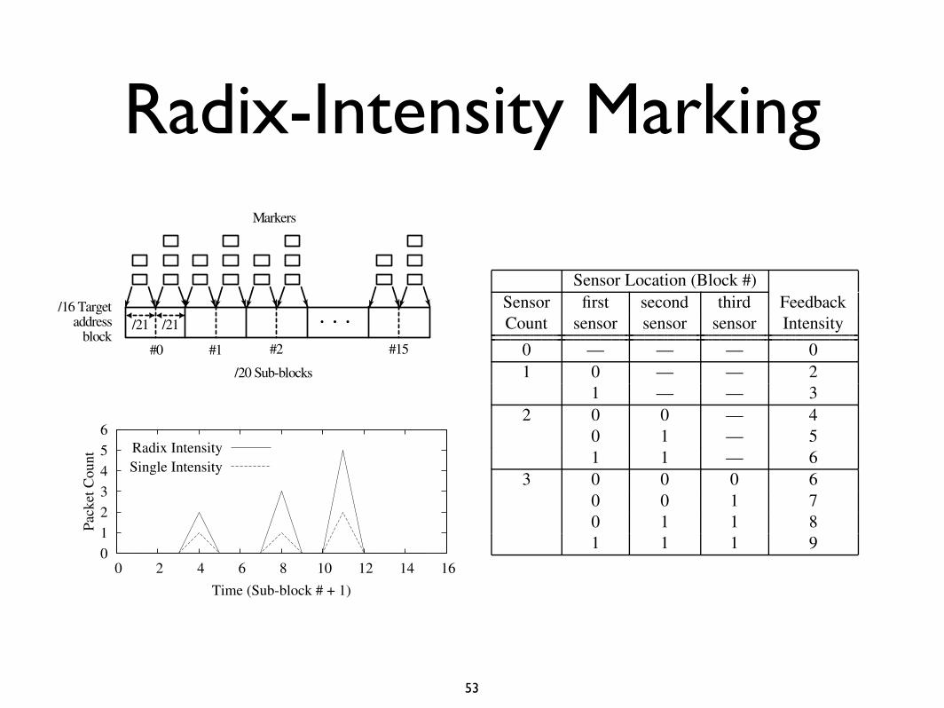
Radix-Intensity Marking
4.3.3 Uniform Intensity MarkingIn uniform-intensity marking, all addresses are markedwith the same intensity. For example, let’s assume thatwe are marking a /16 address block that is known to con-tain several sensors. We divide the original block into16 smaller /20 sub-blocks. Then we mark each of thesesub-blocks using time-series marking, one sub-block pertime unit, marking each address with a single marker.
0 1 2 3 4 5 6
0 2 4 6 8 10 12 14 16
Pack
et C
ount
Time (Sub-block # + 1)
Figure 8: An Example of Uniform-Intensity MarkingFeedback
Figure 8 shows an ideal (no packet loss, and all otherconditions being good) feedback graph from the mark-ing described above. In this figure, the vertical axis rep-resents the packet count and the horizontal axis repre-sents time. We see that there is a spike of height one attime 4, which means that there is one sensor in sub-block#3, since the packet count at time 4 is accumulated be-tween time 3 and time 4, when sub-block #3 was beingmarked. Similarly, there is a spike of height one at time8 and height two at time 11, meaning there is one sensorin sub-block #7 and two sensors in sub-block #10.
4.3.4 Radix-Intensity MarkingIn radix-intensity marking, selected address bits aretranslated into marking intensity, i.e., the number ofpackets for each address. Let us consider the exampleused in the uniform-intensity section above. We exe-cute the same marking procedure, but mark the first /21block within a sub-block with 2 markers, and the second/21 block with 3 markers (Figure 9). Table 1 shows thepossible location of sensors within a sub-block, and howthey are reflected in the feedback intensity.
/16 Target address
block#0 #1 #2
. . .#15
/20 Sub-blocks
Markers
/21 /21
Figure 9: An Example of Radix-Intensity Marking
Sensor Location (Block #)Sensor first second third FeedbackCount sensor sensor sensor Intensity
0 — — — 01 0 — — 2
1 — — 32 0 0 — 4
0 1 — 51 1 — 6
3 0 0 0 60 0 1 70 1 1 81 1 1 9
Table 1: Single Bit (2 for 0 and 3 for 1) Radix-IntensityFeedback for up to 3 sensors in a sub-block.
0 1 2 3 4 5 6
0 2 4 6 8 10 12 14 16
Pack
et C
ount
Time (Sub-block # + 1)
Radix IntensitySingle Intensity
Figure 10: An Example of Radix-Intensity MarkingFeedback
For this example, we further assume that there are nomore than two sensors in each sub-block. Figure 10shows the ideal feedback from this marking with solidlines. The feedback from the uniform-intensity markingis also drawn for comparison in dotted lines. Looking atthe solid line, we notice a spike with height 2 at time 4meaning that there is one sensor in the first half of sub-block #4. There is also a spike with height 3 at time 8meaning that there is one sensor in the second half ofsub-block #7. Another spike spike with height 5 can beseen at time 11 meaning that there are two sensors, onein the first and another in the second half of sub-block#10.
Notice that with uniform-intensity marking, the feed-back would have derived only the numbers of sensors ineach sub-block, while radix-intensity marking was ableto also derive information about the positions of thesesensors within each sub-block. For this example, theradix-intensity marking derived an extra bit of addressinformation.
In radix-intensity marking, the assignment of inten-sity to address bit patterns has to be designed carefullyto minimize the ambiguity during feedback translation.The above example used intensities 2 and 3 for a singlebit. As shown in Table 1, this assignment allows unique
53
Radix Port Marking
If multiple ports are available for marking, a port pair can be assigned to toggle an address bit on or off.
54
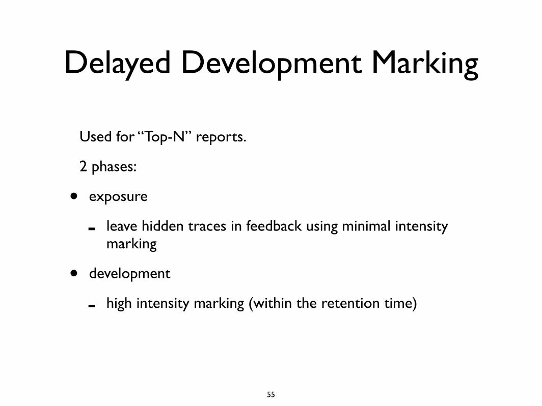
Delayed Development Marking
Used for “Top-N” reports.
2 phases:
• exposure
- leave hidden traces in feedback using minimal intensity marking
• development
- high intensity marking (within the retention time)
55
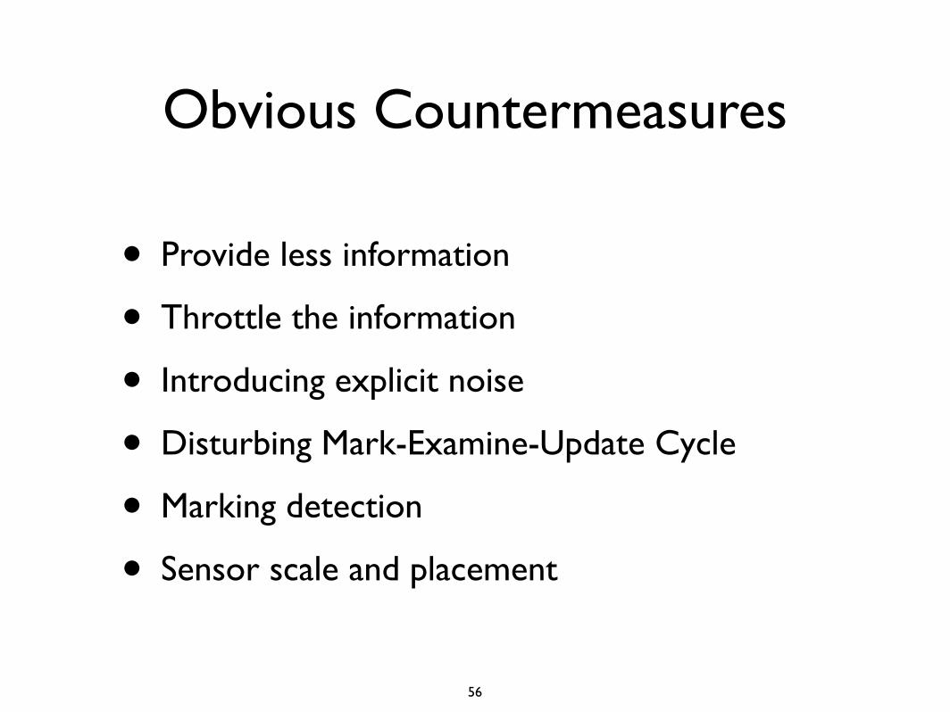
Obvious Countermeasures
• Provide less information
• Throttle the information
• Introducing explicit noise
• Disturbing Mark-Examine-Update Cycle
• Marking detection
• Sensor scale and placement
56
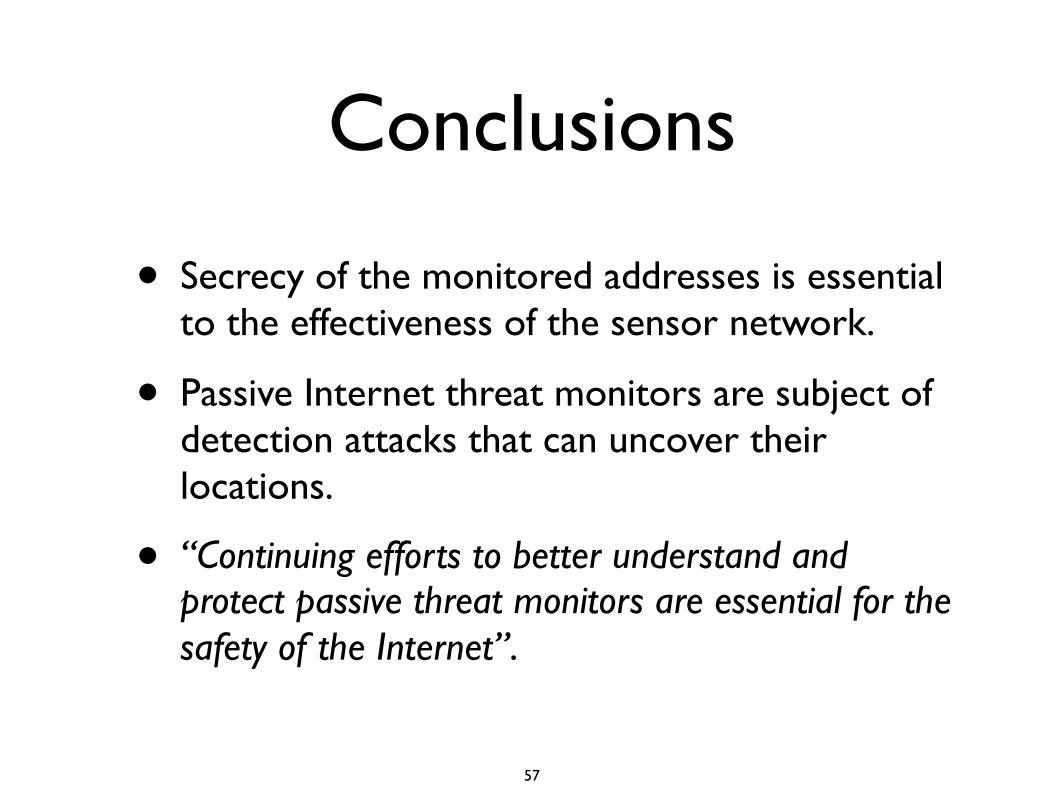
Conclusions
• Secrecy of the monitored addresses is essential to the effectiveness of the sensor network.
• Passive Internet threat monitors are subject of detection attacks that can uncover their locations.
• “Continuing efforts to better understand and protect passive threat monitors are essential for the safety of the Internet”.
57

Can we do this without “summaries”?


