Rheological Model for Wood

Mohammad Masoud Hassania, Falk K. Wittela, Stefan Heringa, and HansJ. Herrmanna

aComputational Physics for Engineering Materials, IfB, ETH Zurich,Schafmattstrasse 6, CH-8093 Zurich, Switzerland

November 6, 2014

Abstract

Wood as the most important natural and renewable building material plays animportant role in the construction sector. Nevertheless, its hygroscopic characterbasically affects all related mechanical properties leading to degradation of materialstiffness and strength over the service life. Accordingly, to attain reliable designof the timber structures, the influence of moisture evolution and the role of time-and moisture-dependent behaviors have to be taken into account. For this purpose,in the current study a 3D orthotropic elasto-plastic, visco-elastic, mechano-sorptiveconstitutive model for wood, with all material constants being defined as a func-tion of moisture content, is presented. The corresponding numerical integrationapproach, with additive decomposition of the total strain is developed and imple-mented within the framework of the finite element method (FEM). Moreover topreserve a quadratic rate of asymptotic convergence the consistent tangent opera-tor for the whole model is derived.

Functionality and capability of the presented material model are evaluated byperforming several numerical verification simulations of wood components underdifferent combinations of mechanical loading and moisture variation. Additionally,the flexibility and universality of the introduced model to predict the mechanicalbehavior of different species are demonstrated by the analysis of a hybrid woodelement. Furthermore, the proposed numerical approach is validated by comparisonsof computational evaluations with experimental results.

Keywords: Hardwood, Constitutive model, Moisture, Multi-surface plasticity,Numerical integration, Mechano-sorption, Moisture-stress analysis.

1 Introduction

Wood application, in particular in form of engineered or composite wood elements, hassignificantly increased as structural building material. Only recently, structural woodencomponents such as glulam or laminated veneer lumber (LVL) entirely or partially (hy-brid) out of hardwood aim for or obtained general technical approvals. The advantagesof hardwood such as beech, oak, or ash are obvious: high strength and stiffness allow for

1

smaller cross-section or span width compared to softwood, resulting in increased dimen-sional stability, load-carrying capacity and finally more freedom for design. In spite of theaforementioned advantages, unfortunately the strong hygric dependence of basically allmechanical properties render many innovative ideas futile. In addition, time-dependentphenomena like long-term visco-elastic creep [20,26] and mechano-sorption under chang-ing environmental conditions [1,14,21] can accelerate degradation of stiffness and strengthover the life-time of a structural wood component and result in the loss of capacity andconsequently structural integrity even after being in use for decades. Realistic long-termpredictions of the mechanical performance of hardwood or hybrid elements under ex-ternal mechanical and climatic loading should be a central concern for assuring both -serviceability and safety of timber structures. It is a common practice today to disregardmoisture, creep, plasticity, and mechano-sorption for technical approvals, not becausethey are insignificant, but because of difficulties in their experimental assessment, thatis challenging due to a high degree of coupling, time consuming due to low diffusivity,and in some cases simply impossible. For these reasons and in order to attain effectivedesign criteria for new products, the development and characterization of an authenticmoisture-dependent constitutive material model for different wood species and the robustimplementation of its corresponding rheological model in broadly used non-linear finiteelement (FE) environments is of great importance.

Non-linear numerical models for wood, in particular with long-term character are veryrare due to the need of species and moisture-dependent mechanical parameters. Severalexperimental and theoretical constitutive wood material models with different ambientrelative humidity (RH) and mechanical loading were proposed. A review on the generaluse of FE in wood analysis was published by Meckerle [31], while other authors focus onreviewing proposed rheological models [13, 48]. In principle the sources for non-linearitylike plasticity, creep, or mechano-sorption are covered to quite different extent. Creepand mechano-sorption were addressed in [2,3,7,12,28,35,40], while others focus on elasto-plastic behavior, disregarding time dependency [11,30,36]. A comprehensive constitutivemodel comprising all potentially activated mechanical responses as a function of moisturecontent for different species is still missing. However it is the basis for numerical simula-tions that grant insight into the long-term behavior of structural elements of hardwoods,softwoods and hybrid ones.

Here a 3D orthotropic material model with moisture content is presented, where allinstantaneous and time-dependent deformation mechanisms are considered. The cor-responding numerical implementation of the material model is written as a material(UMAT) subroutine for the use within a finite element environment. The material modelcan be utilized as the basis of any moisture-stress analysis, for non-linear fracture me-chanical problems established on the cohesive zone model and applications of interfaceelements, or de-bonding simulations under different combinations of service loadings andchanging environmental conditions. The manuscript is organized as follows: First allpartial deformations as components of the total strain together with their correspondingrheological formulations are described from a thermodynamical point of view. Then thedescription of moisture transfer inside wood elements and the principles of moisture-stressanalysis are summarized. Section 3 focuses on the iterative time integration approach andpresents all theoretical formulations needed for the numerical implementation of the ma-terial model in the context of a finite element environment. The verification of the func-tionality and applicability as well as the experimental validation of the material model

2

are shown in Section 4 by means of examples. Finally the generality and flexibility ofthe proposed constitutive model are demonstrated by a hygro-mechanical simulation fora typical hybrid glulam beam made of European beech and Norway spruce in Section 5.

2 Description of the hygro-mechanical constitutive

model

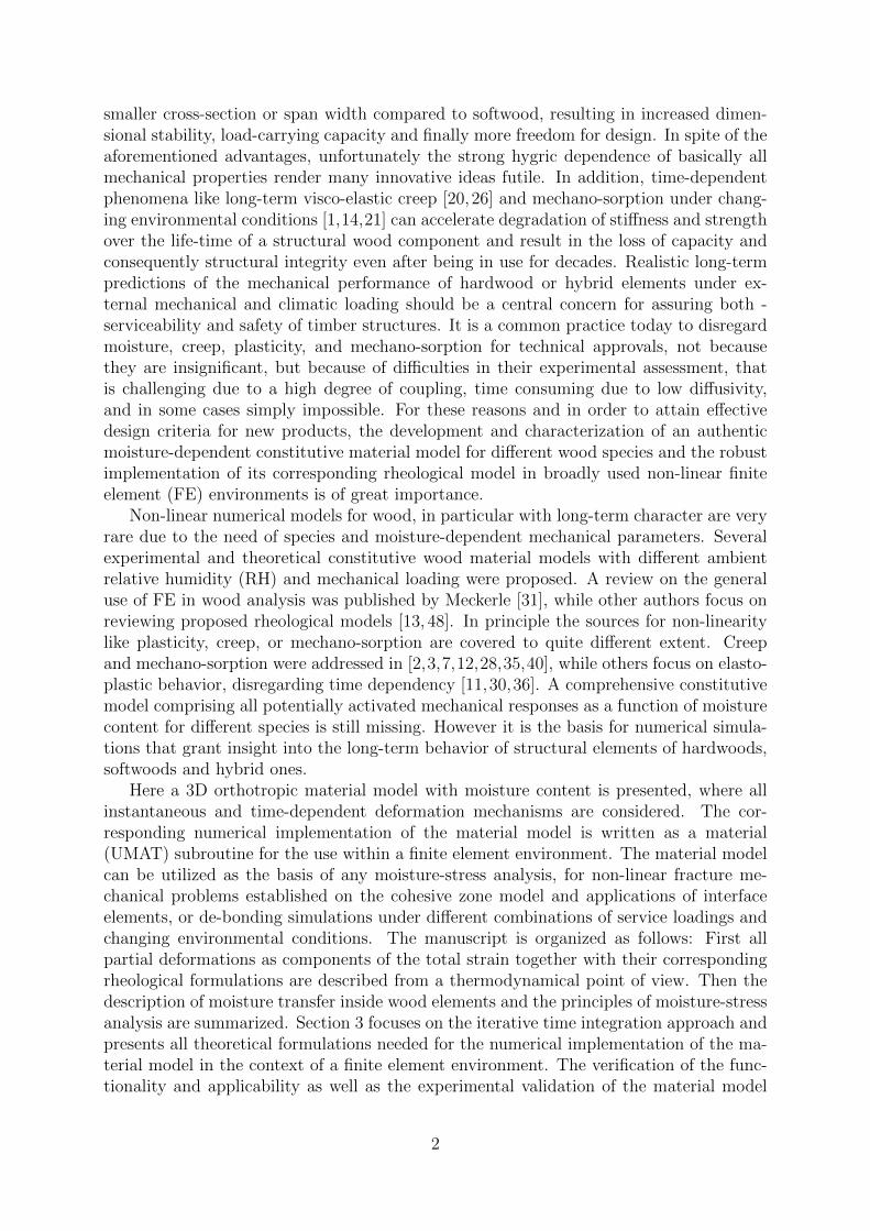
Due to the cellular nature of wood and its growth, wood is in general anisotropic. How-ever for cut sections distant from the center of the stem, it is usually considered as anorthotropic material with three major axes, namely longitudinal along fiber direction,radial and tangential in the plane perpendicular to grain (see Fig. 1). The curvature ofthe growth rings can be considered by defining the orthotropic material in a cylindricalcoordinate system. To capture the consequences of the hygric behavior, all mechanicalproperties along the anatomical directions have to be consequently expressed as a functionof moisture content.

Figure 1: Definition of the local orthotropy directions of wood.

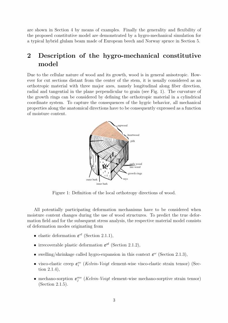
All potentially participating deformation mechanisms have to be considered whenmoisture content changes during the use of wood structures. To predict the true defor-mation field and for the subsequent stress analysis, the respective material model consistsof deformation modes originating from

• elastic deformation εel (Section 2.1.1),

• irrecoverable plastic deformation εpl (Section 2.1.2),

• swelling/shrinkage called hygro-expansion in this context εω (Section 2.1.3),

• visco-elastic creep εvei (Kelvin-Voigt element-wise visco-elastic strain tensor) (Sec-tion 2.1.4),

• mechano-sorption εmsj (Kelvin-Voigt element-wise mechano-sorptive strain tensor)(Section 2.1.5).

3

ε

elε ωε 1

nvei

iε

=∑plε

veiε

msjε

σ0C

ωα iC

iτ

jC

jµ

,c lf

lH

Plastic Elastic Visco-elastic Mechano-sorption Hygro-expansion

1

mmsj

jε

=∑

σ

Figure 2: Schematic illustration of the constitutive material model.

In general a total strain tensor ε is defined that accumulates the respective contribu-tions in the way: (see [7, 12, 28] and Fig. 2)

ε = εel + εpl + εω +n∑i=1

εvei +m∑j=1

εmsj . (1)

From a thermodynamical perspective [7,12,28], the free energy function, ψ, is defined as:

ψ = ψ(T, ω, ε, εpl, εvei , εmsj , αl) = φ(T, ω) + ψel + ψve + ψms +

1

2

r∑l=1

qlαl. (2)

Here φ(T, ω) is a general expression for the thermal energy and since in the present studythe effect of temperature on the mechanical response of the material is ignored, it isnot further considered. ψel specifies elastic strain energy, ψve and ψms represent energyaccumulated in the visco-elastic and mechano-sorptive elements:

ψel =1

2εel : C0 : εel, ψve =

1

2

n∑i=1

εvei : Ci : εvei , ψms =1

2

m∑j=1

εmsj : Cj : εmsj , (3)

with the elastic stiffness tensor C0, and the element-wise visco-elastic and mechano-sorptive stiffness tensors Ci and Cj. Finally, the last term of the right-hand-side ofEq. (2) designates the isotropic hardening energy, which appears during the evolution ofirrecoverable plastic deformations. In the following, all partial strains based on an additivedecomposition of the total strain in addition to their associated thermodynamic drivingstresses are described following [12,28]. It should be noted the proposed hygro-mechanicalconstitutive model is formulated and implemented for infinitesimal strains. It means theapplication of the material model in case of large deformations, non-linear visco-elasticity,or damage phenomenon is not relevant.

4

2.1 Description of mechanical behavior

2.1.1 Elastic deformation

The elastic deformation represents the scleronomous linear and fully recoverable materialbehavior. After differentiating the free energy function Eq. (2) with respect to the totalstrain, the corresponding rheological relation is obtained as:

σ =∂ψ

∂ε= C0 :

(ε− εpl − εω −

n∑i=1

εvei −m∑j=1

εmsj

)= C0 : εel. (4)

Consequently one can write εel = C−10 : σ, with the orthotropic elastic compliance ten-sor C−10 constituted by 9 independent material engineering constants given as

C−10 =

1ER

−νTR

ET

−νLR

EL0 0 0

−νRT

ER

1ET

−νLT

EL0 0 0

−νRL

ER

−νTL

ET

1EL

0 0 0

0 0 0 1GRT

0 0

0 0 0 0 1GRL

0

0 0 0 0 0 1GTL

. (5)

The non-zero off-diagonal terms of the elastic compliance matrix are mutually equal whichis referred to as reciprocal dependencies and can be written by the following relations:

νRTER

=νTRET

,νRLER

=νLREL

,νTLET

=νLTEL

. (6)

Note that all engineering constants depend on the moisture level. They can be fitted bylinear and third degree polynomial functions of moisture content ω for the properties Pband Ps associated with the species European beech and Norway spruce, respectively viaparameters bx, sy (x = 0,1 and y = 0,...,3): Pb = b0 + b1ω and Ps = s0 + s1ω + s2ω

2 +s3ω

3 valid from oven-dry condition to the fiber saturated state. The relevant coefficientsfor describing material constants utilized in the definition of the compliance tensors aresummarized in the B in Table B.

2.1.2 Plastic deformation

Wood is a hygroscopic material with strong dependence of stiffness and strength on themoisture content. It is therefore prone to accumulate irrecoverable deformations even un-der combinations of moderate load with simultaneous moisture increase. The tendency ofimportant hardwood species, such as European beech for high moisture sorption amplifiesthe drop of mechanical properties - strength in particular - what can result in excessiveplastic deformations. Hence for reliable and meaningful predictions of the behavior ofwood in constructions, it is advisable to consider irrecoverable constituents of the totalstrain.

In the last decade, significant efforts were made for describing the elasto-plastic me-chanical behavior of wood based on the progress in metal plasticity. Experiments wereconducted for uni- and bi-axial loading under tension and compression [4–6,29] for differ-ent species and moisture content that lead to the following striking observations:

5

(a) Failure of wood under tensile or shear loading exhibits localized brittle fracture,however under compression, pronounced inelastic behavior is witnessed.

(b) Under compression, two consecutive regimes are observed [27, 41], namely cellularcollapse, and for larger inelastic strains densification or compaction of the collapsedcells [5, 6].

(c) Plastic hardening in different anatomical directions is only weakly coupled, sincedifferent orientation dependent micro-mechanical mechanisms act on the cellularscale.

These experimental observations have consequences for elasto-plastic models, the shapeand type of yield surfaces and their evolution. Simple models use a single deformable3D ellipsoidal yield surface [28, 30], however despite of the advantage of having a closedsurface with C2-consistency, observations (a,c) point at the limited validity of such anapproach. The other extreme is given by a multi-surface approach, where seven distinctfailure mechanisms and subsequently seven yield flow criteria comprising three tensile andthree compressive failures along orthotropy directions together with one shear failure areconsidered [41]. The constructed surface is only C0-consistent, requiring procedures forstress states that lie on intersections, since the evolution of the individual surfaces is notcoupled, leading to 7 internal state variables. The model is basically a generalization ofthe presented plane stress model [27] to 3D. In principle the brittle tensile response canbe treated in the framework of plasticity as a smeared crack, however other approachese.g., using cohesive elements are more stable [38,42]. In later versions, therefore only the3 compressive surfaces were used by the authors [42]. A further reduction was proposedby [19,38,39] with smooth corners (C1-continuity) and a combined evolution of all surfacesbeing described by a single strain-type internal state variable.

This study uses a yield surface similar to Ref. [42], namely a three-dimensional or-thotropic non-smooth multi-surface plasticity model (C0-continuity) consisting of threeindependent failure mechanisms along anatomical directions for compressive loading. Toinclude the role of changing moisture content on the development of plasticity, all rel-evant strength values and respective hardening parameters are defined to be moisturedependent. The transition between elastic and inelastic domains in the stress space ischaracterized by three yield functions in the same form as the second-order polynomialfailure criterion proposed by Ref. [47] as follows:

fl(σ, αl, ω) = al(ω) : σ + σ : bl(ω) : σ + ql(αl, ω)− 1, l = R, T, L. (7)

αl denotes the strain-type internal state variable related to every anatomical direction, aland bl resemble the strength tensors to be defined in the following, and eventually ql is ascalar value for plastic hardening.

Quantitative experimental data for the moisture dependence of the plastic hardeningbehavior is rather sparse. To characterize the hardening behavior we therefore adopt amathematical approach proposed by Ref. [19] with a modified form of Ramberg-Osgoodequations [43] that was successfully applied to the compressive behavior of Europeanbeech at various moisture contents. Unidirectional moisture-dependent isotropic harden-ing laws are applied that describe measured constitutive behavior under uni-axial com-pression along three anatomical orientations. The term ”unidirectional” emphasizes theindependence of the hardening phenomenon of different failure mechanisms from each

6

other, described above. The moisture-dependent hardening responses derived from themodified Ramberg-Osgood curves (see Ref. [19]) are approximated by exponential func-tions as follows:

ql(αl, ω) = (β0lω + β1l)(1− e−β2lαl)/fc,l(ω), (8)

in accordance with the available experimental results. Here l denotes the orientation R,T, L, β0l, β1l, and β2l are material constants, and fc,l(ω) is the compressive strength ofthe material at the current level of moisture content. Since the last term of the right-hand-side of Eq. (7) is equal to one, the current value of the hardening, i.e., ql(αl, ω) mustbe normalized by the compressive strengths to make it consistent with the dimension ofthe yield criterion expression. All parameters needed for the calculation of hardeningfunctions for spruce and beech are summarized in the B in Table B. Note that in thiswork contrary to Refs. [27,41] the densification regime is omitted (observation(b)).

Strength values are described by a linear dependence on the moisture content ω.Analogous to Table B, all corresponding properties for beech and spruce are calculatedas Pb = (zb0ω+zb1) and Ps = (zs0ω+zs1), respectively where zb0, zb1, zs0, and zs1 are givenin Table B in the B. The first index in the symbolic presentations of the strength values(c, t, s) implies compressive, tensile, and shear, while the second one indicates either oneof the anatomical directions or the corresponding plane. In the following, all strengthtensors, i.e., al and bl required for the formulation of the yield criterion belonging to eachfailure mechanism based on the approach introduced in Ref. [41] and in accordance withthe RTL alignment of the orthotropic material coordinate system are given. bl are diagonalmatrices with entries outside the main diagonal being zero. Note that all compressive yieldstresses in the definition of the strength tensors are accompanied by a minus sign.

Compression in radial direction

aR =[

1fc,R

0 0 0 0 0]T, for European beech and Norway spruce,

bR = diag[

0, 0.0805f2c,T

, −0.1490fc,Lft,L

, 0.1080f2s,RT

, 0.1125f2s,RL

, 0.0705f2s,TL

], for European beech,

(9a)

bR = diag[

0, 0.4000f2c,T

, −0.2500fc,Lft,L

, 0.4000f2s,RT

, 0.3300f2s,RL

, 0.3300f2s,TL

], for Norway spruce.

(9b)

Compression in tangential direction

aT =[

0 1fc,T

0 0 0 0]T, for European beech and Norway spruce,

bT = diag[

0.0805f2c,R

, 0, −0.1490fc,Lft,L

, 0.1080f2s,RT

, 0.1125f2s,RL

, 0.0705f2s,TL

], for European beech,

(10a)

bT = diag[

0.4000f2c,R

, 0, −0.2500fc,Lft,L

, 0.4000f2s,RT

, 0.3300f2s,RL

, 0.3300f2s,TL

], for Norway spruce.

(10b)

7

Compression in longitudinal direction

aL =[

0 0 1fc,L

0 0 0]T, for European beech and Norway spruce,

bL = diag[

0.0665f2c,R

, 0.0665f2c,T

, 0, 0.0675f2s,RT

, 0.0855f2s,RL

, 0.0530f2s,TL

], for European beech,

(11a)

bL = diag[

0.3300f2c,R

, 0.3300f2c,T

, 0, 0.2500f2s,RT

, 0.2500f2s,RL

, 0.2500f2s,TL

], for Norway spruce.

(11b)

The scalar coefficients in the numerator of the diagonal components of the strengthmatrices bl are weighting factors which following Ref. [41] can be adjusted to the respectivespecies. To make an adaptation from spruce (s) to beech (b), we replace the respectivestrength value of the denominator by f s = f b ·

(f b12/f

s12

)what corresponds to a scaling

of the scalar values with strength value ratios at ω = 12%. Until today, bi-axial tests forbeech have not been published in literature, hence a final justification for this adaptationassumption is not possible. In Fig. 3 the boundary between the linear elastic domain andthe non-linear behavior of the material, based on strength tensors al and bl at ω = 12%,and for (ql = 0) is shown. Because of the three-dimensional representation of the stresstensor, the demonstration of all yield surfaces for any arbitrary stress state through oneindividual image is not feasible. Accordingly, in Fig. 3 (left) a two-dimensional illustrationof the yield conditions under planar state of stress in the R-L plane, i.e., (σT = σRT =σTL = 0) and for principal normal stresses (σRL = 0) is depicted. Fig. 3 (right) shows athree-dimensional visualization of the failure surfaces for the situation in which principaldirections of stress and axes of the local material coordinate system are coincident (σRT =σRL = σTL = 0).

Figure 3: Left: 2D illustration of the yield surfaces in the R-L plane and for σRL = 0.Right: 3D visualization of the boundaries between elastic and plastic domains in theprincipal stress space. Both are illustrated for ql = 0 at ω = 12%.

By now, all moisture-dependent parameters needed for the description of the rate-independent multi-surface plasticity material model are introduced. The general algo-rithm for the numerical implementation of the above-mentioned model is explained indetail in Refs. [22,43]. Now we focus on a concise description of the principles of the evo-lution equations for irrecoverable deformations in the context of non-smooth multi-surfaceplasticity. The constitutive relation of the plastic deformation under the assumption of a

8

standard associative plasticity is described by the following formula known as flow rule,usually referred to as Koiter’s rule [24]:

εpl =r∑l=1

γl∂σfl(σ, αl, ω) =r∑l=1

γl(al(ω) + 2bl(ω) : σ). (12)

Here r denotes the number of active yield mechanisms. Similarly with associative hard-ening, the evolution equation corresponding to the hardening law takes the form

α =r∑l=1

γl∂qfl(σ, αl, ω) =r∑l=1

γl. (13)

In Eqs. (12) and (13), γl are plastic consistency parameters, which fulfill the followingKuhn-Tucker complementary requirements:

γl ≥ 0, fl(σ, αl, ω) ≤ 0, γlfl(σ, αl, ω) = 0, (14)

together with the consistency condition:

γlfl(σ, αl, ω) = 0. (15)

For an assumed number of active yield constraints radm and a given state of stress andinternal hardening variable(s)

Sadm := {l ∈ {R, T, L} | fl(σ, αl, ω) = 0} , (16)

the Kuhn-Tucker complementary conditions also known as loading/unloading require-ments can be restated for multi-surface plasticity as the following [43]:

Condition 1. If fl(σ, αl, ω) < 0 or fl(σ, αl, ω) = 0 and fl(σ, αl, ω) < 0, subsequently γl =0, which define the case of elastic loading or unloading, where plastic strains alongwith hardening variable(s) do not change.

Condition 2. If fl(σ, αl, ω) = 0 and fl(σ, αl, ω) = 0, then γl ≥ 0, which specifies theplastic loading and subsequently the evolution of plastic deformation and respectiveinternal variable(s).

Accordingly, based on Eq. (16) and an expanded form of the loading/unloading condi-tions, 1 ≤ r ≤ radm representing the number of active yield conditions reads as:

Sact :={l ∈ Sadm | fl(σ, αl, ω) = 0

}. (17)

To summarize, flow role Eq. (12) and hardening law Eq. (13) in combination withKuhn-Tucker complementary requirements form a set of non-linear equations with γl

as unknown variables. The corresponding solution can be realized through an iterativenumerical procedure like a Newton-Raphson scheme [12,28,43].

9

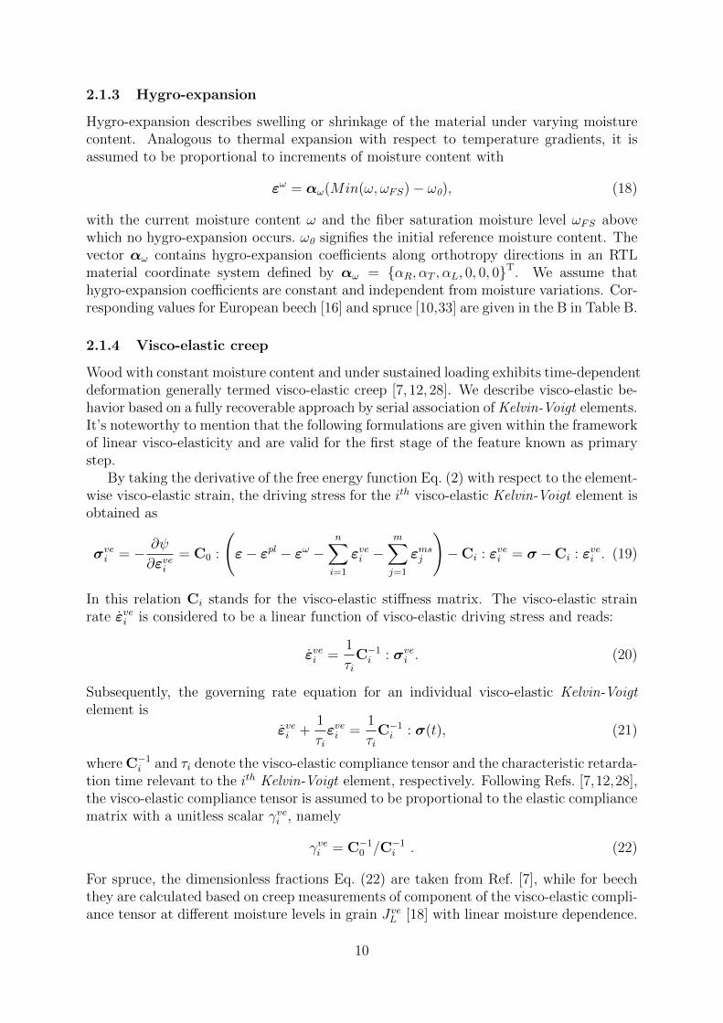
2.1.3 Hygro-expansion

Hygro-expansion describes swelling or shrinkage of the material under varying moisturecontent. Analogous to thermal expansion with respect to temperature gradients, it isassumed to be proportional to increments of moisture content with

εω = αω(Min(ω, ωFS)− ω0), (18)

with the current moisture content ω and the fiber saturation moisture level ωFS abovewhich no hygro-expansion occurs. ω0 signifies the initial reference moisture content. Thevector αω contains hygro-expansion coefficients along orthotropy directions in an RTLmaterial coordinate system defined by αω = {αR, αT , αL, 0, 0, 0}T. We assume thathygro-expansion coefficients are constant and independent from moisture variations. Cor-responding values for European beech [16] and spruce [10,33] are given in the B in Table B.

2.1.4 Visco-elastic creep

Wood with constant moisture content and under sustained loading exhibits time-dependentdeformation generally termed visco-elastic creep [7, 12, 28]. We describe visco-elastic be-havior based on a fully recoverable approach by serial association of Kelvin-Voigt elements.It’s noteworthy to mention that the following formulations are given within the frameworkof linear visco-elasticity and are valid for the first stage of the feature known as primarystep.

By taking the derivative of the free energy function Eq. (2) with respect to the element-wise visco-elastic strain, the driving stress for the ith visco-elastic Kelvin-Voigt element isobtained as

σvei = − ∂ψ

∂εvei= C0 :

(ε− εpl − εω −

n∑i=1

εvei −m∑j=1

εmsj

)−Ci : εvei = σ −Ci : εvei . (19)

In this relation Ci stands for the visco-elastic stiffness matrix. The visco-elastic strainrate εvei is considered to be a linear function of visco-elastic driving stress and reads:

εvei =1

τiC−1i : σvei . (20)

Subsequently, the governing rate equation for an individual visco-elastic Kelvin-Voigtelement is

εvei +1

τiεvei =

1

τiC−1i : σ(t), (21)

where C−1i and τi denote the visco-elastic compliance tensor and the characteristic retarda-tion time relevant to the ith Kelvin-Voigt element, respectively. Following Refs. [7,12,28],the visco-elastic compliance tensor is assumed to be proportional to the elastic compliancematrix with a unitless scalar γvei , namely

γvei = C−10 /C−1i . (22)

For spruce, the dimensionless fractions Eq. (22) are taken from Ref. [7], while for beechthey are calculated based on creep measurements of component of the visco-elastic compli-ance tensor at different moisture levels in grain JveL [18] with linear moisture dependence.

10

For a serial combination of four Kelvin-Voigt elements, Table B in the B provides theparameters that describe the moisture dependent longitudinal component of the creepcompliance tensor for the ith Kelvin-Voigt element:

JveiL = (Ji1ω + Ji0)(1− e−t/τi). (23)

The ratio of the longitudinal component of the elastic compliance tensor 1EL

with this valuegives the fraction γvei relevant to each Kelvin-Voigt element. Note that due to sparseexperimental data, it is a common practice to apply the fraction γvei measured in thegrain also to the cross-grain directions. Additionally, the same value of the characteristictime (viscosity) along the grain is utilized for other anatomical directions as well. Henceretardation times are defined isotropically.

Following Refs. [7,12,28] by integrating Eq. (21), the element-wise visco-elastic strainresponse of the ith Kelvin-Voigt element reads

εvei,n+1 = εvei,n exp(−∆t

τi) +

∫ tn+1

tn

C−1i : σ(t)

τiexp(−tn+1 − t

τi) dt, (24)

for a stress driven problem, with the time step ∆t = tn+1− tn and the visco-elastic straintensors εvei,n+1, ε

vei,n at time tn+1 and tn, respectively.

2.1.5 Mechano-sorptive creep

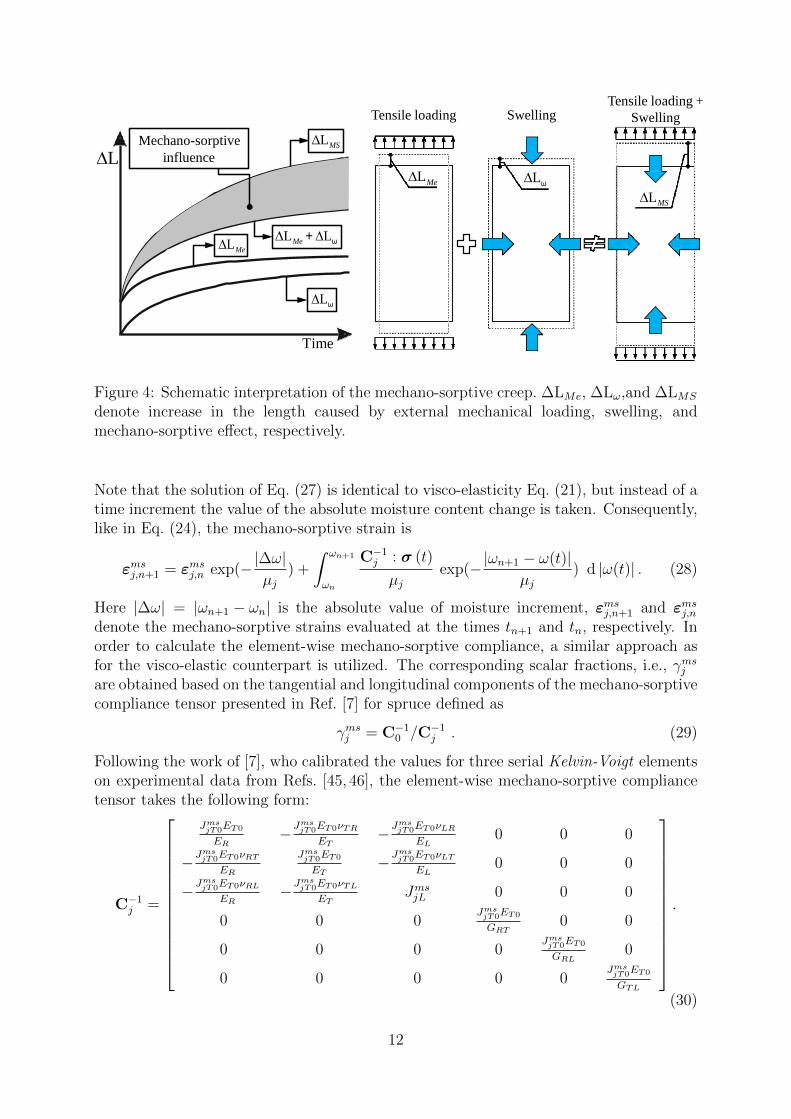
The effect that the observed deformation of a loaded specimen under changing moisturecontent is remarkably higher than the deformation of a loaded specimen under constantclimatic conditions superimposed by the deformation of an unloaded specimen undervarying moisture level is known as mechano-sorptive creep (see Fig. 4). Experimentalstudies for spruce can be found in Refs. [15, 32, 37], while for beech such studies are stillmissing.

For the numerical description of mechano-sorption in principle Kelvin-Voigt type el-ements are used [7, 12, 28]. In Refs. [12, 28] plasticity is part of mechano-sorption, whilein the formulation by Ref. [7] that we follow, it is an independent strain contribution.After differentiating the free energy function Eq. (2) with respect to the element-wisemechano-sorptive creep strain, the corresponding driving stress becomes

σmsj = − ∂ψ

∂εmsj= C0 :

(ε− εpl − εω −

n∑i=1

εvei −m∑j=1

εmsj

)−Cj : εmsj = σ −Cj : εmsj ,

(25)where Cj stands for the mechano-sorptive stiffness tensor. For characterizing mechano-sorption, a rate equation quite similar to the one of the visco-elastic creep Eq. (20) isapplied:

εmsj =|ω|µj

C−1j : σmsj . (26)

Here µj is called characteristic moisture analogous to the characteristic retardation time invisco-elasticity and C−1j designates the tensor of mechano-sorptive compliance respective

to the jth Kelvin-Voigt element. By inserting Eq. (25) in Eq. (26) and rearranging,the constitutive relation for a single mechano-sorptive Kelvin-Voigt type element can bewritten as

εmsj +|ω|µjεmsj =

|ω|µj

C−1j : σ(t). (27)

11

Mechano-sorptive ∆L influence

∆LMS

Tensile loading

∆LMe

Swelling

∆Lω

Tensile loading + Swelling

∆LMS

∆LMe ∆LMe + ∆Lω

∆Lω

Time

Figure 4: Schematic interpretation of the mechano-sorptive creep. ∆LMe, ∆Lω,and ∆LMS

denote increase in the length caused by external mechanical loading, swelling, andmechano-sorptive effect, respectively.

Note that the solution of Eq. (27) is identical to visco-elasticity Eq. (21), but instead of atime increment the value of the absolute moisture content change is taken. Consequently,like in Eq. (24), the mechano-sorptive strain is

εmsj,n+1 = εmsj,n exp(−|∆ω|µj

) +

∫ ωn+1

ωn

C−1j : σ (t)

µjexp(−|ωn+1 − ω(t)|

µj) d |ω(t)| . (28)

Here |∆ω| = |ωn+1 − ωn| is the absolute value of moisture increment, εmsj,n+1 and εmsj,ndenote the mechano-sorptive strains evaluated at the times tn+1 and tn, respectively. Inorder to calculate the element-wise mechano-sorptive compliance, a similar approach asfor the visco-elastic counterpart is utilized. The corresponding scalar fractions, i.e., γmsjare obtained based on the tangential and longitudinal components of the mechano-sorptivecompliance tensor presented in Ref. [7] for spruce defined as

γmsj = C−10 /C−1j . (29)

Following the work of [7], who calibrated the values for three serial Kelvin-Voigt elementson experimental data from Refs. [45, 46], the element-wise mechano-sorptive compliancetensor takes the following form:

C−1j =

JmsjT0ET0

ER−Jms

jT0ET0νTR

ET−Jms

jT0ET0νLR

EL0 0 0

−JmsjT0ET0νRT

ER

JmsjT0ET0

ET−Jms

jT0ET0νLT

EL0 0 0

−JmsjT0ET0νRL

ER−Jms

jT0ET0νTL

ETJmsjL 0 0 0

0 0 0JmsjT0ET0

GRT0 0

0 0 0 0JmsjT0ET0

GRL0

0 0 0 0 0JmsjT0ET0

GTL

.

(30)

12

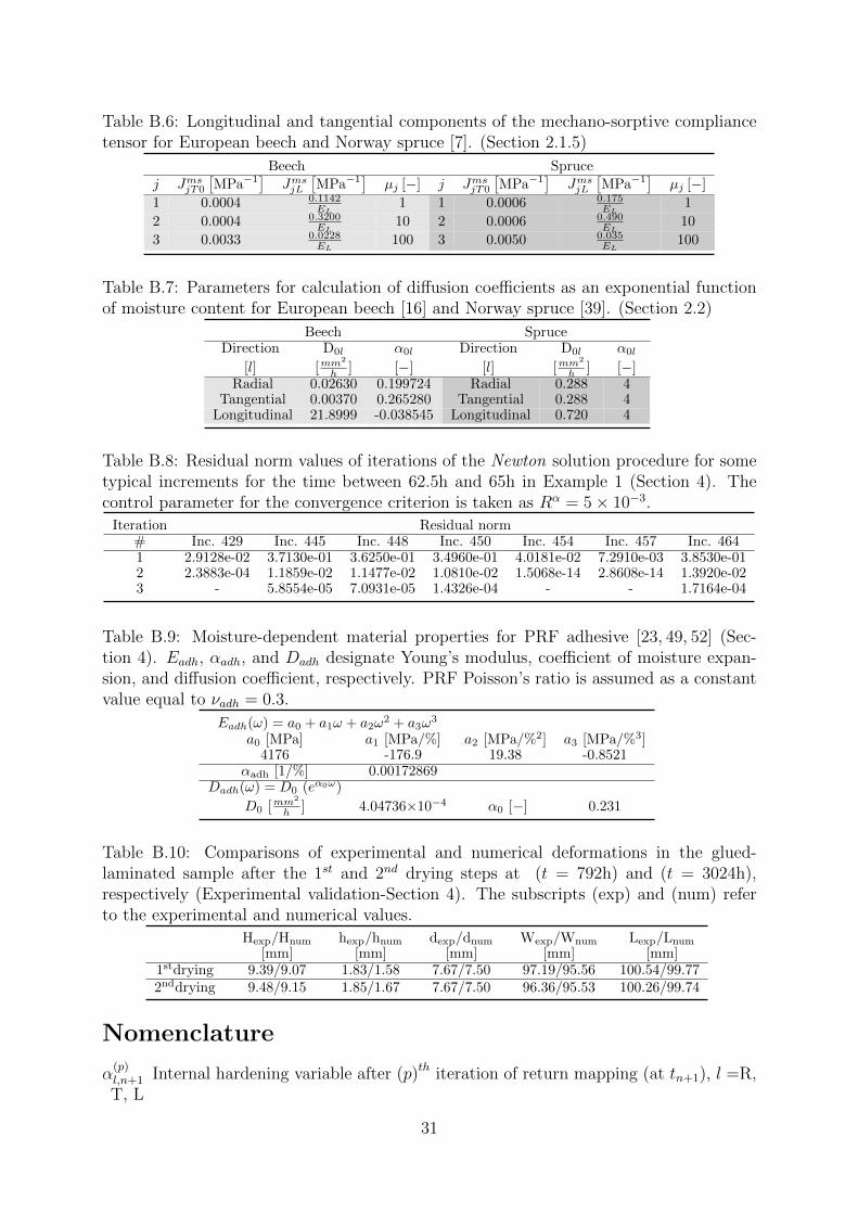
The values corresponding to JmsjT0 and JmsjL together with the characteristic moistures µj aresummarized in the B in Table B.6. Due to lack of data on the mechano-sorptive behavior ofbeech, the corresponding values of the mechano-sorptive compliance tensor are calculatedby scaling the spruce values by the ratio of densities of the two species (470/720) [34].

2.2 Moisture-stress analysis

Due to the importance of moisture fields and gradients for the behavior of wood, mois-ture transport is essential for simulations. In this work mechanical and thermal fieldsdo not influence moisture transport, so the problem is only partially coupled. Further-more we assume moisture transport inside the porous material wood to be dominatedby diffusive transport [10]. Experimental observations of moisture transport below fibersaturation show more correspondence with non-Fickian behavior [25,50], or multi-Fickiandiffusion [8]. In the present work for the sake of simplicity and also because of insuffi-cient details regarding either non-Fickian or multi-Fickian formulations, Fick ’s law formoisture transfer is employed.

In accordance with the Fick ’s first law the body moisture flux is given by

Jbω = −D∇c, (31)

where Jω is body moisture flux vector, D denotes the matrix of diffusion coefficients, c =ρ0ω is the water concentration, ρ0 the oven-dry wood density, and ω is again the moisturecontent in [%]. Fick ’s second law expresses the change of the concentration with respectto the time. In a general form and for changing diffusion coefficients, the time variationof concentration is written as:

∂c

∂t= ∇.(D∇c). (32)

For constant density Eq. (32) simplifies to

∂ω

∂t= ∇.(D∇ω). (33)

In general, mathematical formulations of moisture diffusion and heat transfer are similar.The Fourier equations of heat transfer are

JT = −K∇T, and (ρcT )∂T

∂t= ∇.(K∇T ) , (34)

with the heat flux JT , density ρ, specific heat cT and temperature T , as well as thematrix of thermal conductivity coefficients K. The analogy between Eqs. (33) and (34)is preserved when (ρcT ) = 1, rendering thermal analysis capabilities of FE packages validfor moisture transport simulations. In this work, the diffusion process is assumed tobe uncoupled among anatomical directions and subsequently, the matrix of orthotropicdiffusion coefficients is defined as:

D = diag[

DR DT DL

]. (35)

The diffusion coefficients are considered to be moisture-dependent and can be describedby exponential laws as a function of moisture, namely

Dl(ω) = D0l (eα0lω), (36)

where l=R, T, and L. All parameters required to calculate moisture-dependent diffusioncoefficients for spruce and beech [16,39] are summarized in the B in Table B.7.

13

3 Numerical implementation of the moisture-dependent

rheological model

To implement the material model with the presented rheological behavior in the frame-work of a FE simulation, an incremental, iterative numerical approach is needed [7,12,28]with time increments (∆t = tn+1 − tn). In the following, subscripts (•)n indicate a stateat the beginning of a time step, whereas the subscript (•)n+1 refers to the end of the timeincrement. The stress update algorithm is based on the assumption that at time t = tn,the state of the material is available to be able to calculate the corresponding solutionat time t = tn+1 by means of an incremental update procedure. In detail the state vari-ables are the moisture distribution, the total strain including all five corresponding partialconstituents, internal plastic hardening variables and the total stress tensor. The individ-ual algorithmic tangent operators associated with each deformation mode are computedseparately and then, by incorporating all single Jacobians, the tangent operator for the en-tire model is obtained following Refs. [7, 12, 28]. Additionally, the total strain incrementand the amount of moisture content change are needed for the iteration. The hygro-expansion strain tensor

(εωn+1

)and the total strain tensor (εn+1) at the end of the time

increment are estimated and needed for the incrementation as well, using the old tangentoperators. At each integration point the total stress tensor and total Jacobian matrix,meaning the algorithmic tangent operator for the whole constitutive model, are updatedat the end of the time increment. In addition, the values of state variables in terms ofelastic strain (εel), irrecoverable plastic deformation (εpl) along with related strain-typehardening variable(s) (αl), viscoelastic strain tensor respective to every Kelvin-Voigt ele-ment (εvei ), and all element-wise mechano-sorptive strain tensors (εmsj ) have to be updatedfor the next increment. A brief overview of the iterative algorithm utilized for the de-composition of the total strain (ε) and the incremental procedure for the update of totalstress and all state variables can be summarized as below:

1. Stage 1: Data initialization Based on the iterative algorithm for the stress up-date, all state variables are set to their corresponding values from the last convergediteration of the previous increment as:

εve(k=0)i,n+1 = εvei,n, ε

ms(k=0)j,n+1 = εmsj,n . (37)

The superscript k refers to the (k)th iteration of the considered increment. The firstone (k = 0) therefore is identical to the converged solution of the former increment.

2. Stage 2: Plastic deformation In the next step, the possible development ofirrecoverable deformation by plastic strain is examined. For this purpose a two-stepreturn-mapping algorithm known as elastic predictor/plastic corrector based on thegeneral multi-surface closest point projection approach is used [22, 43]. According

to the trial state of elastic strain at the end of the time increment(εel(Trial)n+1

)the

position of the stress state with respect to the evolved yield surfaces is checked. Ifplastic loading is the case, the trial state of stress calculated from the trial elasticstrain is projected onto the current yield surface (see Fig. 5).

The plastic strain and respective internal variable(s) also need to be initialized asfollows:

εpl(Trial)n+1 = ε

pl(k=0)n+1 = εpln , α

(Trial)l,n+1 = α

(k=0)l,n+1 = αl,n . (38)

14

1nσ +

11

pnσ++

1pnσ +

11nσ +

( )1

Trialnσ +

Elastic domain

nσ

Current yield surface

Plastic corrector: Elastic predictor:

Figure 5: Schematic representation of the concept of elastic predictor/plastic correctorin the context of the closest point projection iteration algorithm, based on Ref. [43].

From a theoretical point of view, the trial state of elastic strain is achieved bysuppressing the evolution of plastic flow within the time increment. As a conse-quence, ε

el(Trial)n+1 and all corresponding state variables in the trial state read as [43]:

εel(Trial)n+1 =

(εn+1 − εpl(Trial)n+1 − εωn+1 −

n∑i=1

εve(k)i,n+1 −

m∑j=1

εms(k)j,n+1

), (39)

σ(Trial)n+1 =

(C0,n+1 : ε

el(Trial)n+1

), (40)

q(Trial)l,n+1 = ql

(α(Trial)l,n+1 , ωn+1

)= ql(αl,n, ωn+1), (41)

f(Trial)l,n+1 = fl

(σ

(Trial)n+1 , q

(Trial)l,n+1 , ωn+1

), (42)

subsequently, based on the last expression for the yield functions if all f(Trial)l,n+1 ≤ 0

the deformation is purely elastic and consistency parameters of all yield mechanismsdo not change (∆γl = 0 for l = R,T,L), but if at least for one of them f

(Trial)l,n+1 > 0,

the time step is plastic and the plastic strain increment along with changes of thestrain hardening variable(s) and changes in the consistency parameters have to beevaluated. Therefore, by defining

εel(p)n+1 =

(εn+1 − εpl(p)n+1 − εωn+1 −

n∑i=1

εve(k)i,n+1 −

m∑j=1

εms(k)j,n+1

), (43)

σ(p)n+1 =

(C0,n+1 : ε

el(p)n+1

), (44)

q(p)l,n+1 = ql

(α(p)l,n+1, ωn+1

), (45)

f(p)l,n+1 = fl

(σ

(p)n+1, q

(p)l,n+1, ωn+1

), (46)

and by means of an iterative return-mapping algorithm (i.e., plastic corrector) in-cremental plastic deformations, hardening variable(s), and consistency parameter(s)

15

associated with the active yield surface(s) are obtained. Note that superscripts p inEq. (43) refer to the pth iteration of the return mapping algorithm. Consequently,iterative formulations concerning update of the state variables and consistency pa-rameters are

εpl(p+1)n+1 = ε

pl(p)n+1 + ∆ε

pl(p)n+1 , (47)

α(p+1)l,n+1 = α

(p)l,n+1 + ∆α

(p)l,n+1, (48)

∆γl(p+1)n+1 = ∆γ

l(p)n+1 + δ∆γ

l(p)n+1, for all l ∈ Sact . (49)

∆γln+1 denotes the non-rate form of the consistency parameter, whereas δ∆γln+1

signifies the corresponding increment. At the end of the return mapping itera-tion, (p+ 1) is set to (p) and the convergence of the iteration is checked. A plasticresiduum vector, consisting of components related to the iterative evolution of theplastic strain tensor and of hardening variable(s):

Rpl(p)n+1 :=

−εpl(p)n+1 + εpln

−α(p)n+1 +αn

+r∑

l ∈ Sact

∆γl(p)n+1

∂σfl(σ(p)n+1, α

(p)l,n+1, ωn+1)

∂qfl(σ(p)n+1, α

(p)l,n+1, ωn+1)

(50)

is computed for the convergence check. Now the values of all active yield func-tions are recalculated using the updated stress tensor and hardening variable(s) viaEq. (7). If

f(p)l,n+1 := fl(σ

(p)n+1, α

(p)l,n+1, ωn+1) < TOL1 for all l ∈ Sact , and

∥∥∥Rpl(p)n+1

∥∥∥ < TOL2,

(51)is not fully fulfilled, the procedure loops to the next iteration. Otherwise, the currentiteration has converged and consequently, the definite increments of the plastic straintensor, as well as the hardening variable(s) are obtained. Now all state variablesrelevant to the plastic part of the total strain are updated to the new values at theend of the time step, namely

εpln+1 = εpln + ∆εpln+1, αl,n+1 = αl,n + ∆αl,n+1, for all l ∈ Sact . (52)

3. Stage 3: Stress calculation Now the driving stress in the current iteration ofthe general additive decomposition scheme can be calculated. Taking the straincomponents and the total strain tensor at the end of the increment, the elasticcontribution is

εel(k)n+1 =

εn+1 − εpl(k)n+1 − εωn+1 −

n∑i=1

εve(k)i,n+1 −

m∑j=1

εms(k)j,n+1 , if ε

pl(k)n+1 6= 0,

εn+1 − εωn+1 −n∑i=1

εve(k)i,n+1 −

m∑j=1

εms(k)j,n+1 , if ε

pl(k)n+1 = 0.

(53)

With the calculated elastic strain, the stress tensor at the (k)th iteration of the stressupdate increment is

σ(k)n+1 =

(C0,n+1 : ε

el(k)n+1

). (54)

16

In a next step, the tangent operator for the whole serial model has to be given.For this reason, all individual Jacobians from the 3-4 deformation mechanisms areevaluated separately and assembled to a total algorithmic tangent operator [7,12,28].Since this step is crucial for the convergence of the entire implementation, a detailedexplanation is given in the A. With the total tangent operator CT

n+1, the iterativechange of the total stress is calculated by the expression

∆σ(k)n+1 = −CT

n+1 :

(Rel +

n∑i=1

Rvei +

m∑j=1

Rmsj

)(k)

n+1

. (55)

The residual vectors belonging to each deformation mechanism are defined as:

Rel(k) =

C−10,n+1 : σ

(k)n+1 −

(εn+1 − εpl(k)n+1 − εωn+1 −

n∑i=1

εve(k)i,n+1 −

m∑j=1

εms(k)j,n+1

), if ε

pl(k)n+1 6= 0,

C−10,n+1 : σ(k)n+1 −

(εn+1 − εωn+1 −

n∑i=1

εve(k)i,n+1 −

m∑j=1

εms(k)j,n+1

), if ε

pl(k)n+1 = 0,

(56)

Rve(k)i =

{εvei,n exp (−ξi) + Tven (ξi) C−1i,n : σn + Tven+1 (ξi) C−1i,n+1 : σ

(k)n+1 − ε

ve(k)i,n+1

},

(57)

Rms(k)j =

{εmsj,n exp (−ξj) + Tmsn (ξj) C−1j,n : σn + Tmsn+1 (ξj) C−1j,n+1 : σ

(k)n+1 − ε

ms(k)j,n+1

}.

(58)

4. Stage 4: Visco-elastic and mechano-sorptive deformation Based on thepre-calculated incremental stress tensor Eq. (55) and all decoupled residual vectorsrelated to all individual deformation modes Eqs. (56-58), the change of visco-elasticstrains in conjunction with the variation of mechano-sorptive deformations for thecurrent iteration of the stress update algorithm are determined. Accordingly, thevisco-elastic and mechano-sorptive creep strain increments ∆ε

ve(k)i,n+1 and ∆ε

ms(k)j,n+1 are

evaluated via the following relationships

∆εve(k)i,n+1 = R

ve(k)i + Tven+1 (ξi) C−1i,n+1 : ∆σ

(k)n+1 , for i = (1, ..., n) ,

∆εms(k)j,n+1 = R

ms(k)j + Tmsn+1 (ξj) C−1j,n+1 : ∆σ

(k)n+1 , for j = (1, ...,m) , (59)

that are derived based on the definition of respective algorithmic operators (seeA). Consecutively, all state variables for all element-wise visco-elastic and mechano-sorptive creep deformations are updated at the end of the ongoing iteration usingthe expression

εve(k+1)i,n+1 = ε

ve(k)i,n+1 + ∆ε

ve(k)i,n+1, ε

ms(k+1)j,n+1 = ε

ms(k)j,n+1 + ∆ε

ms(k)j,n+1 . (60)

The iterative procedure is completed by comparing a generalized residual vec-tor R

(k+1)n+1

R(k+1)n+1 =

{Rel(k+1)n+1 R

ve(k+1)i,n+1 · · ·R

ms(k+1)j,n+1 · · ·

}T, (61)

17

composed of all recomputed deformation-based residual vectors Eqs. (56-58), or

more precisely its norm up to a tolerance level. If∥∥∥R(k+1)

n+1

∥∥∥ ≤ TOL3 the iterative

scheme is converged and the solution obtained in the (k+1)th iteration is regarded as

the final response of the current increment. Otherwise, if∥∥∥R(k+1)

n+1

∥∥∥ > TOL3, (k+ 1)

is changed to (k) and stages 2-4 are repeated. After convergence, all values of thestate variables related to the visco-elastic and mechano-sorptive strains, as well asthe elastic deformation Eq. (53) are substituted by the updated ones:

εvei,n+1 = εvei,n + ∆εvei,n+1, εmsj,n+1 = εmsj,n + ∆εmsj,n+1. (62)

These updated state values will be considered as initial values for the next timestep.

4 Verification of the material model

A set of three numerical examples is calculated that verifies the capability and efficiency ofthe proposed 3D constitutive model for the prediction of realistic behavior for short-termand long-term responses under combined moisture and mechanical loading. The examplesare selected in such a way that different deformation components act in an isolated andcombined way under uni- and multi-axial loading, as well as for restrained swelling. Allexamples use the material properties given in the B for European beech (Fagus sylvaticaL.). Furthermore, this section is complemented with an experimental verification.

Example 1 - Uni-axial loading: In a first simple example, a cubic sample with edgelength 40mm is studied. The model uses three confining symmetry planes, reducing theedge length to 20mm (see Fig. 6 (left)). Hence it is allowed to swell or shrink freelyduring moisture variations and hygro-expansions do not lead to residual stresses. Sincethe dimensions are quite small compared to the ones of a stem, the curvature of growthrings is ignored by assigning an orthotropic material behavior to the system that is definedin a Cartesian coordinate system with axes aligned along the cube edges. The geometry isdiscretized by 512 quadratic brick elements (C3D20) and loaded by a uniform compressionin radial direction. Simultaneously a homogeneous moisture distribution can be applied(see Fig. 6 (right)). The pressure and moisture content ω are chosen in a way that allpotential components of the total strain are addressed and can be distinguished clearlyduring the 7 stages:

• Stage 1 0-5h: The sample is at standard climate, i.e., 65% RH resulting in ω1=12%.The pressure is ramped up to 10MPa during 5 hours,

• Stage 2 5-55h: for the next 50 hours all conditions are kept constant,

• Stage 3 55-60h: within the next 5 hours, pressure is increased from 10 to 16MPa,while ω1 = 12% =const.,

• Stage 4 60-135h: at constant load, ω is going through 5 cycles of wetting anddrying, each lasting 15 hours. For 2.5h ω1 = 12%, then ramped up to ω2 = 18%within 2.5h, held constant for 5 hours, ramped down from ω2 to ω1 for 2.5h, heldconstant for 2.5h, a.s.o..

18

• Stage 5 135-140h: At ω1 the load is completely removed during 5h and will remainthis way for the rest of the simulation.

• Stage 6 140-200h: For the next 60 hours all conditions are kept constant.

• Stage 7 200-290h: Finally six more moisture cycles like in Stage 4, but withoutmechanical loading are imposed.

RRσ

Moisture flow R

T L

RRσ

Stage1 2 3 74 5 6

Figure 6: Left: Geometry and finite element model of the wood cubic specimen. Right:Amplitudes of exerted radial compressive stress and moisture distribution on the woodblock sample. (Example 1)

The resulting strain along the radial direction for the loading in the 7 stages is illus-trated in Fig. 7. In order to observe the development of all partial strains in an easyto interpret way, the hygro-expansion strain is subtracted from the total strain and theremaining value, called swelling/shrinkage-modified strain, is shown in Fig. 7 (left). Forthe different stages we observe:

• Stage 1 0-5h: Linear elastic behavior dominates.

• Stage 2 5-55h: Increase in visco-elastic creep is noticed.

• Stage 3 55-60h: Plastic deformation starts as the compressive strength of thematerial along radial direction (i.e., -13.4MPa) is reached. The radial yield criterionis activated, material starts to flow, and the irrecoverable plastic deformation evolvesas the material simultaneously hardens until the yield surface reaches 16MPa.

• Stage 4 60-135h: During the first moisture increase from ω1=12(%) to ω2=18(%),the material strength values degrade and consequently further plastic deformation,even under fixed external loading, evolves (see Fig. 7 (right)). The repetition ofmoistening in the following cycles just leads to a comparably small increase in theirreversible part of the total strain. The increase of strain during the moisture cyclesis therefore dominated by mechano-sorptive creep. Note that the general response ofthe material model representing the simultaneous interaction of fixed level of loading

19

and varying moisture content shows a good agreement with experimental observa-tions of mechano-sorptive creep reported by Refs. [21, 45, 46]. It can be noticedthat both moistening and de-moistening leads to the increase of mechano-sorptivedeformation and generally, the material behavior demonstrates an ascending trendwhich implies that mechano-sorptive creep is accumulated over time.

• Stage 5 135-140h: During unloading, the instantaneous elastic response is imme-diately compensated.

• Stage 6 140-200h: Visco-elastic creep is partly recovered.

• Stage 7 200-290h: Partial recovery of mechano-sorptive creep.

It can be concluded that retrieval of the visco-elastic deformation requires adequate time,while the recovery of the mechano-sorption is achieved by moisture variation. As canbe observed in Fig. 7 (left) even though the external pressure is removed, a remarkableamount of strain stays in the material. A part of this remaining deformation consists oftime-dependent responses and another part is due to the occurrence of irreversible plasticdeformation.

Figure 7: Left: Time evolution of all constituents of the total strain along radial direction.Right: Development of radial irrecoverable plastic strain and mechano-sorptive creep.(Example 1)

In addition, mechanical responses of the wood block along two other directions, i.e.,tangential and longitudinal are also given in Fig. 8. Although no mechanical loading is ap-plied along these two directions, significant lateral strains are generated. Contrary to theradial direction and as a consequence of the implemented multi-surface plasticity, whereall failure mechanisms in each anatomic direction are independent, no plastic deformationscan occur in T- and L-direction. Therefore all deformations are fully recoverable aftertime and moisture variations under zero external loading. The offset between the two di-rections can be explained by the fact that beech is much stiffer parallel than perpendicularto grain. Additionally, since the longitudinal entry of the mechano-sorptive compliance

20

tensor was calculated differently than the other components (see Section 2.1.5), the gen-eral mechano-sorptive response of the material model parallel to growth direction differsqualitatively from the corresponding behavior perpendicular to grain.

Figure 8: Evolution of swelling/shrinkage-modified strains along T- and L-direction. (Ex-ample 1)

Remarks on convergence The classical Newton-Raphson scheme is employed to solvenon-linear problems within the framework of FE environment at which the material modelhas been implemented. Therefore, regarding the performance and the rate of convergenceof the proposed computational algorithm, application of consistent tangent operator is ofgreat significance. Convergence is evaluated in terms of residual control parameter (Rα),which is calculated as the fraction of the largest residual in the equilibrium equation forthe field displacement to the mean value of the conjugate force flux. Here, the conver-gence criterion is assumed as 5×10−3 which would appear rather stringent for engineeringapplications, but to achieve precise solutions to non-linear problems such a small toler-ance is inevitable. Table B.8 in the B shows the computational effort for some typicalincrements during moistening phase of the first moisture cycle for t =62.5 to 65h. As itcan be observed clearly from the data given in Table B.8, the quadratic convergence rateof the implemented material model is obvious. At most three iterations are sufficient tomeet the convergence tolerance in spite of increase in the moisture content resulting inthe variation of model operator in every increment and appearance of further non-linearbehavior. Although it was supposed that such a strict convergence tolerance imposesa very difficult condition to fulfill, via this numerical example it is illustrated that theconvergence is satisfied after few number of iterations. Due to application of consistentJacobian, the general robustness of the computational model is preserved.

Example 2 - Multi-axial loading: To evaluate the model behavior under arbitrarycombinations of load with multiple yield surfaces activated, a tri-axial state of stress isimposed on the same specimen, but now with load in all anatomical directions (see Fig. 9(left)). Boundary conditions, as well as loading history are identical to the first example

21

(see Fig. 6) only that the load in tangential direction is scaled by a factor of 0.4 and theone in longitudinal by a factor of 4.

RRσ

Moisture flow R

T L

RRσ

LLσ

TTσTTσ

Figure 9: Left: Illustration of the tri-axial state of stress. Right: Time evolution ofirreversible plastic strains along all three anatomical directions. (a) and (b) denote iso-hygric loading and the moistening phase of the 1st moisture cycle, respectively. (Example2)

For the second simulation the same interpretations as for the first example apply, con-cerning the evolution of all instant and time-dependent mechanical behavior. However,in contrast to example 1, all three yield mechanisms will be activated and consequently,irrecoverable plastic deformations evolve along all three anatomic directions simultane-ously. The resulting plastic deformations are illustrated in Fig. 9 (right). As visible, thetangential direction deforms more plastically, since it is the least stiff orientation. Fur-thermore, it should be noted that due to the application of a consistent tangent operator,the quadratic rate of convergence is preserved, even when multiple failure mechanisms areactive.

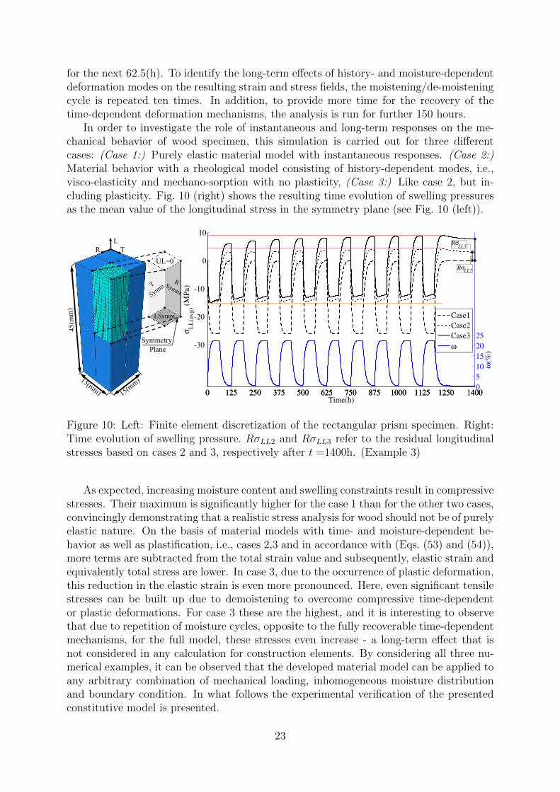
Example 3 - Restrained swelling: As a last example, we simulate restrained swelling,as this is an experimentally studied loading case of practical relevance. We observe theevolution of the swelling pressure, as the rectangular sample of size 45mm×15mm×15mm(L×R×T) is exposed to a cycling moisture change (see Fig. 10). This transient numericalsimulation aims to assess the practical behavior of wood components in terms of moisturedistribution, all possibly emerging deformation mechanisms, moisture-dependent plastifi-cation in particular, and associated stress fields, generated during moistening processes.Hence moisture transport is calculated based on the procedure outlined in Section 2.2.Like in the previous examples, we make use of the symmetric nature of the problem,and additionally to the three symmetry planes, we impose a non-moving boundary inL-direction at the top surface. The moisture content cycles from oven-dry condition(ω1 = 0.5%) in 62.5h to a state with 95% RH, in ω2 = 22.5% close to the fiber saturation,only that moisture diffuses into the system from the exposed surfaces. Then, to observethe permanent deformations, the moisture content is again returning back to ω1 = 0.5%

22

for the next 62.5(h). To identify the long-term effects of history- and moisture-dependentdeformation modes on the resulting strain and stress fields, the moistening/de-moisteningcycle is repeated ten times. In addition, to provide more time for the recovery of thetime-dependent deformation mechanisms, the analysis is run for further 150 hours.

In order to investigate the role of instantaneous and long-term responses on the me-chanical behavior of wood specimen, this simulation is carried out for three differentcases: (Case 1:) Purely elastic material model with instantaneous responses. (Case 2:)Material behavior with a rheological model consisting of history-dependent modes, i.e.,visco-elasticity and mechano-sorption with no plasticity, (Case 3:) Like case 2, but in-cluding plasticity. Fig. 10 (right) shows the resulting time evolution of swelling pressuresas the mean value of the longitudinal stress in the symmetry plane (see Fig. 10 (left)).

Figure 10: Left: Finite element discretization of the rectangular prism specimen. Right:Time evolution of swelling pressure. RσLL2 and RσLL3 refer to the residual longitudinalstresses based on cases 2 and 3, respectively after t =1400h. (Example 3)

As expected, increasing moisture content and swelling constraints result in compressivestresses. Their maximum is significantly higher for the case 1 than for the other two cases,convincingly demonstrating that a realistic stress analysis for wood should not be of purelyelastic nature. On the basis of material models with time- and moisture-dependent be-havior as well as plastification, i.e., cases 2,3 and in accordance with (Eqs. (53) and (54)),more terms are subtracted from the total strain value and subsequently, elastic strain andequivalently total stress are lower. In case 3, due to the occurrence of plastic deformation,this reduction in the elastic strain is even more pronounced. Here, even significant tensilestresses can be built up due to demoistening to overcome compressive time-dependentor plastic deformations. For case 3 these are the highest, and it is interesting to observethat due to repetition of moisture cycles, opposite to the fully recoverable time-dependentmechanisms, for the full model, these stresses even increase - a long-term effect that isnot considered in any calculation for construction elements. By considering all three nu-merical examples, it can be observed that the developed material model can be applied toany arbitrary combination of mechanical loading, inhomogeneous moisture distributionand boundary condition. In what follows the experimental verification of the presentedconstitutive model is presented.

23

Experimental validation of an uncross-wise laminated sample: To investigatethe practical behavior of adhesively bonded wood elements under varying relative hu-midity, a three-layered uncross-wise laminated European beech specimen was exposed tomoisture variations. Initially conditioned at 95% RH layers were glued together usingPRF (phenol resorcinol formaldehyde) adhesive. Subsequently, the composite sample wasplaced inside a climate box with varying RH comprising of three consecutive steps: 1)de-moistening from 95% RH to 2% RH; 2) re-moistening to 95% RH; 3) another de-moistening to 2% RH. At the end of each de-moistening cycle, the moisture-inducedwarping and sample dimensions were measured by means of a dial gauge.

The FEM model consists of five layers: three lamellae for wood substrates and twoadhesive layers with a thickness of 0.1 mm (see Fig. 11).

XZY

Encastre

UY=0

UX&UY=0

1

23

1 25.02 2 23.69 3 4.18

20.1

40.1

2

Figure 11: Left: Finite element model of the uncross-wise laminated sample. Right:Applied boundary conditions and Cartesian material coordinates. Indices refer to thelayers. All dimensions are in mm.

The variation of the RH inside the climate box is converted to the equivalent moisturecontent by means of the sorption isotherm curves for both European beech and PRFadhesive [51]. These values are applied as time-dependent surface conditions to all externalfaces of the FE model during the moisture analysis. Using the described wood rheologicalmodel and a purely linear elastic isotropic behavior for the adhesive layers, the moisture-induced stress and the deformation fields are computed subsequently. Note that theadhesive properties are functions of moisture content as well with all parameters beingsummarized in Table B.9 in the B.

The comparison of simulation results with experimental observations gives excellentagreement, implying that the material model performs well for practical applications (seeFig. 12 and Table B.10).

The quantitative comparison of moisture related deformations between experiment andsimulation (Table B.10) gives excellent agreement considering that the utilized materialproperties are general values and do not consider the large variations common to wood.By having a more detailed look at the Table B.10 it can be realized that the dimension”H”, called here as cup deformation, has identically increased in experiment+simulationfor the second de-moistening compared to the first one. This augmentation is due to time-and history-dependent deformation mechanisms. Note that even though in this examplethe difference in ”H” is only 0.1 mm, it increases with the number of cycles and canfor different configurations, like cross-lamination or hybrid components add to reaching

24

Bottom side

L

numh

numW

numHnumd

expW

exph

expH

expd

Figure 12: Deformed shape at 2% RH. (Top) 3D view and (bottom) side view of exper-iment and simulation, naming the measurement points for quantitative comparisons inthe Table B.10.

critical values.

5 Application example: Hybrid wood elements

Combinations of different materials and wood species are a promising approach to over-come design limitations that result in extreme cross sections of structural elements madeof softwood or in expensive solutions for load transfer from other elements perpendicularto grain, just to give two examples. The combination of beech and spruce has recentlyattracted significant attention due to a general technical approval for such a hybrid glulamelement. It is interesting to note that neither plastic behavior, nor long-term effects didplay a role in the approval procedure. To demonstrate the capability of the introduced ap-proach, a hybrid glulam beam made of European beech and Norway spruce is considered.Both were adhesively joined at initial moisture content of 10%. The multi-species beam issubjected to changing environmental conditions varying between 50% RH and 90% RH.Although European beech and Norway spruce show different moisture sorption isotherms,due to the small difference between the equivalent moisture contents at mentioned RH asingle value representing the moisture content of the whole beam is considered. The initialmoisture content at 50% RH is estimated as 10% and the new equilibrium moisture levelat 90% RH is approximated as 21%. They are taken as surface conditions for the mois-ture transport simulation. Note that these moisture levels are taken as the mean values ofadsorption and desorption curves for simplicity. The time variation of RH or equivalentlymoisture content is expressed by means of the positive part of the sine function, which

25

varies between 10% to 21% for the duration of one year (365 days).In the simulation, two distinct constitutive models consisting of five deformation mech-

anisms each, related to every wood type are considered. In practice, two material (UMAT)subroutines are defined simultaneously. The adhesive layer between two lamellae is ne-glected and lamellae are considered as different sections of one part, but with distinctmaterial type and individual cylindrical local material coordinate systems, each. Sharednodes therefore have only one value for the moisture content and adhesive bond lines arefully permeable. As illustrated in Fig. 13 (left), the simulated system represents a part ofa hybrid glulam beam consisting of ten 30mm thick and 150mm wide lamellae, all alignedin the longitudinal direction with the top and bottom two made of beech, while the coreis made of six spruce lamellae. In order to avoid modeling the entire length of the beam,a section with the length of 50mm under assumption of generalized plane strain state hasbeen considered. For this purpose, at the top right corner of the cross-section a refer-ence point (R.P.) is defined and the movements of the end plane with red boundaries, i.e.,translation along Z-direction and rotation around X and Y axes are kinematically coupledto the reference point (see Fig. 13 (left)).

(B)

(S)(S)pl

T

(B)plT

XZY

R.P.

End Pl.

(B)(S) Encastre

UY&UZ=0

UX&UY=0

(B)

(B)

(B)

(S)

(S)

(S)(S)(S)

ZSymm

Figure 13: Left: Geometrical dimensions and finite element discretization of the multi-species beam. (B) and (S) designate beech and spruce, respectively. Right: Distributionof tangential plastic strain after one year (t =365 days).

In Fig. 13 (right) the distribution of the plastic deformations along tangential directionis given. It should be noted that plastic strains in each lamella are illustrated based on thecorresponding local material coordinate system. Depending on the position of the centerand the orientation of the assigned local cylindrical coordinate systems, the distributionof the plastic strain varies. As it’s expected and could also be observed in the calculations,the magnitudes of plastic strain in the beech layers are smaller than the counterpart val-ues in the spruce lamellae. Additionally, the plastic deformations are mostly generated

26

near the adhesive bond-lines. This is due to the occurrence of higher stress concentrationin the interface of two adjacent lamellae, resulting from different material properties andmaterial orientations. These stress concentrations, in forms of tension or shear in partic-ular, can lead to the initiation of interfacial cracks that propagate under applied servicemechanical loadings and changing environmental conditions. Subsequently, structuralintegrity and load-carrying capacity are diminished. So, plasticity induced de-bondingcould be considered as a critical failure mode of such laminated structural elements, theconsequences of which have to be taken into account during design stage. By applicationof the annual moisture profile during some consecutive years, the role of both short- andlong-term responses in the mechanical performance of the hybrid element in addition tothe influence of moisture cycles on the development of time- and history-dependent stressstates are captured.

6 Conclusions

In the current study, a comprehensive rheological model for the mechanical behavior ofwood under simultaneous mechanical loadings and varying environmental conditions isintroduced. The considered deformation modes are both short- and long-term responses,namely elastic, plastic, hygro-expansion, visco-elastic creep, and mechano-sorption. Tocharacterize the irrecoverable part of the material response, described as plastic deforma-tion, a general multi-surface plasticity model with three independent failure mechanisms -each one belonging to an anatomical direction under compression - is employed. Moreover,the time-dependent behaviors like visco-elastic and mechano-sorptive creep are simulatedthrough serial association of Kelvin-Voigt elements. In order to consider the inherenthygroscopic character of wood in the assessment of timber structures, all material inputparameters are defined as function of the moisture level. The numerical integration algo-rithm along with the utilized approach for the stress update scheme are established onan iteratively additive decomposition of the total strain. All corresponding rheologicalformulations were developed and implemented into a user-material subroutine (UMAT)within the environment of the finite element method.

The material model was applied to two important wood species, namely Europeanbeech and Norwegian spruce. However due to scarce availability of stress-strain relation-ships under different loading cases and moisture contents, for beech in particular, someproperty adaptation procedures had to be implemented to obtain a full set of materialdata. The functionality and performance of the model and its implementation was eval-uated through several examples for uni- and multi-axial loading, as well as for restrainedswelling. The examples demonstrated the applicability of the presented material modelunder any optional load combination, specifically when more than one failure mechanismis activated. In addition, the validation of the presented material model was carried outby comparison with experimental results in a glued-laminated specimen.

The introduced material model is numerically implemented in a general fashion andcan also be used for other wood species. By application of moisture-dependent materialproperties, the rheological model can easily be adapted to predict the mechanical responseof different wood types. In this respect, the flexibility and efficiency of the material modelhas been proven by simulating a hybrid beech/spruce glulam element. In general, the pro-posed wood constitutive material model can be employed for finite element analysis ofmoisture-induced stresses in adhesively bonded wood elements. Additionally, this model

27

can be considered as a suitable basis for fracture mechanical analyses or can be combinedwith cohesive interface elements to predict the initiation and propagation of interfacialcracks. This way we achieve the goal of attaining more realistic and reliable predictionson mechanical performance of wood elements under any arbitrary combinations of load-ing and moisture content to increase safety and long-term reliability of engineered woodstructures.

7 Acknowledgments

This work was funded by the Swiss National Science Foundation in the National ResearchProgramme NRP 66 - Resource Wood under grant Nr. 406640- 140002: Reliable timberand innovative wood products for structures. We also would like to thank Prof. P. Niemzand Mr. S. Ammann for fruitful discussions.

A Algorithmic tangent operator for the whole model

Purely elastic or elasto-plastic tangent operator: From a rheological point of view,the tangent operator corresponding to the first two elements of the constitutive materialmodel (Fig. 2), namely the elastic spring and the plastic Kelvin element are correlated. Inthe absence of plastic strain, the plastic Kelvin element will be inactive without giving acontribution to the tangent operator. Trivially, the single Jacobian is equal to the elasticstiffness tensor Cel

n+1 = C0,n+1. However in the presence of plastic deformation, bothelastic and plastic elements contribute to the definition of the elasto-plastic algorithmictangent modulus [43]:

Cepn+1 = Ξn+1 −

∑β∈Sact

∑α∈Sact

(Gβαn+1 Nβ,n+1 ⊗Nα,n+1

). (A.1)

Note that ⊗ symbolizes the dyadic product of two vectors and Ξn+1 is the algorithmicmodulus and is given by the following relationship:

Ξn+1 =

[C−10,n+1 +

r∑l=1

∆γln+1∂2σσfl (σn+1, αl,n+1, ωn+1)

]−1=

[C−10,n+1 + 2

r∑l=1

∆γln+1bl,n+1

]−1,

(A.2)and

Nα,n+1 = Ξn+1 : ∂σfα,n+1, (A.3)

where r is the number of active yield surfaces and Gβαn+1 is defined by the succeeding

expression:

Gβαn+1 =

[∂σfβ,n+1 : Ξn+1 : ∂σfα,n+1 + ∂qfβ,n+1 Hβα

n+1 ∂qfα,n+1

]−1. (A.4)

Here Hβαn+1 denotes the βα component of the matrix of hardening moduli Hn+1 filled

with the respective values for every active yield criterion (Hl = ∂ql/∂αl, l = R, T, L).Eq. (A.1) represents the desired description for algorithmic or the equivalently consistenttangent operator which ensures the quadratic rate of asymptotic convergence of the globaliteration. Note that the application of the continuum elasto-plastic moduli yields at mosta linear rate of convergence [28,43,44].

28

Visco-elastic tangent operator: The analytical solution of Eq. (24) under assumptionof linear variation of stress during time increment (∆t = tn+1 − tn) holds as: [28]

εvei,n+1 = εvei,n exp

(−∆t

τi

)+ Tven

(∆t

τi

)C−1i,n : σn + Tven+1

(∆t

τi

)C−1i,n+1 : σn+1. (A.5)

The time functions Tven+1 (ξi) and Tven (ξi) in Eq. (A.5), where ξi = ∆t/τi, are describedas:

Tven+1 (ξi) = 1− 1

ξi(1− exp (−ξi)) , Tven (ξi) = 1− exp (−ξi)− Tven+1 (ξi) . (A.6)

The differential form of Eq. (A.5) after taking the derivative from both sides reads as

dεvei,n+1 = Tven+1

(∆t

τi

)C−1i,n+1 : dσn+1, (A.7)

that can be rearranged to give the general description of the algorithmic visco-elastictangent operator Cve

i,n+1:Cvei,n+1 = Ci,n+1/Tven+1 (ξi) . (A.8)

Mechano-sorptive tangent operator: Based on an approach similar to the one out-lined for visco-elasticity, the response of Eq. (28) can be stated by the following relation-ship:

εmsj,n+1 = εmsj,nexp

(−|∆ω|

µj

)+Tmsn

(|∆ω|µj

)C−1j,n : σn+Tmsn+1

(|∆ω|µj

)C−1j,n+1 : σn+1. (A.9)

Analogous to Eq. (A.6) the moisture functions Tmsn+1 (ξj) and Tmsn (ξj), where ξj = |∆ω| /µj,can be given by the following expressions:

Tmsn+1 (ξj) = 1− 1

ξj(1− exp (−ξj)) , Tmsn (ξj) = 1− exp (−ξj)− Tmsn+1 (ξj) . (A.10)

Similar to the approach taken for the visco-elastic Jacobian, differentiating both sides ofEq. (A.9) and comparing to the standard definition of the tangent operator, leads to thealgorithmic mechano-sorptive tangent

Cmsj,n+1 = Cj,n+1/Tmsn+1 (ξj) . (A.11)

It should be noted that hygro-expansion has no contribution to the definition of thetotal operator. Therefore, after specifying all above-mentioned individual algorithmicoperators, the mathematical description of the total Jacobian, corresponding to the entirematerial model CT

n+1 takes the following form:

CTn+1 =

(Cep −1n+1 +

n∑i=1

Cve −1i,n+1 +

m∑j=1

Cms −1j,n+1

)−1, if ε

pl(k)n+1 6= 0,

(Cel −1n+1 +

n∑i=1

Cve −1i,n+1 +

m∑j=1

Cms −1j,n+1

)−1, if ε

pl(k)n+1 = 0.

(A.12)

B Material properties for European beech and Nor-

wegian spruce

29

Table B.1: Coefficients for moisture-dependent engineering constants for European beech[17] and Norway spruce [10,33]. (Section 2.1.1)

ER ET EL GRT GRL GTL νTR νLR νLT[MPa] [MPa] [MPa] [MPa] [MPa] [MPa] [−] [−] [−](

×10−3) (

×10−3) (

×10−3)

Beech b0 2565.6 885.4 17136.7 667.8 1482 1100 293.3 383.0 336.8b1 -59.7 -23.4 -282.4 -15.19 -15.26 -17.72 -1.012 -8.722 -9.071

Spruce s0 999.64 506.08 12791.75 61.33 762.8 880.75 153.4 232.0 285.7s1 3.61 5.0 15.22 -1.07 5.93 1.39 10.8 -8.6 -41.0s2 -2.09 -1.35 -9.01 -0.06 -1.99 -1.39 0.398 2.8784 7.1907s3 0.0467 0.0297 0.1885 0.0017 0.0477 0.0277 -0.0191 -0.07862 -0.1642

Table B.2: Coefficients for calculation of moisture-dependent hardening stress for Euro-pean beech [9, 19]. (Section 2.1.2)

Direction Beechβ0l β1l β2l

[l] [MPa/%] [MPa] [−]R -0.1123 2.8765 55.29T -0.1411 3.2736 65.56L 0.0 2.5180 95.3

Table B.3: Coefficients for calculation of moisture-dependent strength values for Europeanbeech [16] and Norway spruce [39,41]. (Section 2.1.2)

Strength Beech Sprucezb0 zb1 zs0 zs1

[MPa/%] [MPa] [MPa/%] [MPa]fc,R -0.5789 20.32 -0.270 9.24fc,T -0.2084 7.965 -0.270 9.24fc,L -3.5040 103.9 -2.150 68.8ft,L -1.4650 106.9 -3.275 104.8fs,RT -0.1213 4.982 -0.063 2.585fs,RL -0.3884 15.51 -0.227 9.064fs,TL -0.3861 16.21 -0.178 7.477

Table B.4: Swelling/shrinkage coefficients for European beech [16] and Norway spruce[10,33]. (Section 2.1.3)

Hygro-expansion coefficient αR [1/%] αT [1/%] αL [1/%]Beech 0.00191 0.00462 0.00011Spruce 0.00170 0.00330 0.00005

Table B.5: Coefficients for calculation of moisture- and time-dependent entry of the visco-elastic compliance tensor parallel to grain for European beech [18] and dimensionless scalarparameters for Norway spruce [7]. (Section 2.1.4)

Beech Spruce

i[−] Ji1[MPa−1

]Ji0[MPa−1

]τi [h] i[−] γvei τi [h]

1 1.11e-6 -4.99e-6 0.82 1 1/0.085 2.42 9.84e-7 -5.22e-6 60.86 2 1/0.035 243 8.51e-7 -5.97e-6 8.90 3 1/0.070 2404 2.82e-6 1.03e-5 3427.65 4 1/0.200 2400

30

Table B.6: Longitudinal and tangential components of the mechano-sorptive compliancetensor for European beech and Norway spruce [7]. (Section 2.1.5)

Beech Spruce

j JmsjT0

[MPa−1

]JmsjL

[MPa−1

]µj [−] j JmsjT0

[MPa−1

]JmsjL

[MPa−1

]µj [−]

1 0.0004 0.1142EL

1 1 0.0006 0.175EL

1

2 0.0004 0.3200EL

10 2 0.0006 0.490EL

10

3 0.0033 0.0228EL

100 3 0.0050 0.035EL

100

Table B.7: Parameters for calculation of diffusion coefficients as an exponential functionof moisture content for European beech [16] and Norway spruce [39]. (Section 2.2)

Beech SpruceDirection D0l α0l Direction D0l α0l

[l] [mm2

h ] [−] [l] [mm2

h ] [−]Radial 0.02630 0.199724 Radial 0.288 4

Tangential 0.00370 0.265280 Tangential 0.288 4Longitudinal 21.8999 -0.038545 Longitudinal 0.720 4

Table B.8: Residual norm values of iterations of the Newton solution procedure for sometypical increments for the time between 62.5h and 65h in Example 1 (Section 4). Thecontrol parameter for the convergence criterion is taken as Rα = 5× 10−3.

Iteration Residual norm# Inc. 429 Inc. 445 Inc. 448 Inc. 450 Inc. 454 Inc. 457 Inc. 4641 2.9128e-02 3.7130e-01 3.6250e-01 3.4960e-01 4.0181e-02 7.2910e-03 3.8530e-012 2.3883e-04 1.1859e-02 1.1477e-02 1.0810e-02 1.5068e-14 2.8608e-14 1.3920e-023 - 5.8554e-05 7.0931e-05 1.4326e-04 - - 1.7164e-04

Table B.9: Moisture-dependent material properties for PRF adhesive [23, 49, 52] (Sec-tion 4). Eadh, αadh, and Dadh designate Young’s modulus, coefficient of moisture expan-sion, and diffusion coefficient, respectively. PRF Poisson’s ratio is assumed as a constantvalue equal to νadh = 0.3.

Eadh(ω) = a0 + a1ω + a2ω2 + a3ω

3

a0 [MPa] a1 [MPa/%] a2 [MPa/%2] a3 [MPa/%3]4176 -176.9 19.38 -0.8521

αadh [1/%] 0.00172869Dadh(ω) = D0 (eα0ω)

D0 [mm2

h ] 4.04736×10−4 α0 [−] 0.231

Table B.10: Comparisons of experimental and numerical deformations in the glued-laminated sample after the 1st and 2nd drying steps at (t = 792h) and (t = 3024h),respectively (Experimental validation-Section 4). The subscripts (exp) and (num) referto the experimental and numerical values.

Hexp/Hnum hexp/hnum dexp/dnum Wexp/Wnum Lexp/Lnum

[mm] [mm] [mm] [mm] [mm]1stdrying 9.39/9.07 1.83/1.58 7.67/7.50 97.19/95.56 100.54/99.772nddrying 9.48/9.15 1.85/1.67 7.67/7.50 96.36/95.53 100.26/99.74

Nomenclature

α(p)l,n+1 Internal hardening variable after (p)th iteration of return mapping (at tn+1), l =R,T, L

31

α(Trial)l,n+1 Trial internal hardening variable (at tn+1), l =R, T, L

αω Hygro-expansion coefficients tensor

al,bl Strength tensors

Celn+1/C

epn+1 Elastic/Elasto-plastic tangent operator (at tn+1)

Rel,Rve/msi/j Elastic, i/jth visco-elastic/mechano-sorptive residual vector

σ/σvei /σmsj Total stress/ith visco-elastic stress/jth mechano-sorptive stress tensor

σ(p)n+1 Total stress tensor after (p)th iteration of return-mapping (at tn+1)

σ(Trial)n+1 Trial total stress tensor (at tn+1)

ε/εel/εpl/εω Total strain/Elastic strain/Plastic strain/Hygro-expansion strain tensor

εel(p)/pl(p)n+1 Elastic/Plastic strain tensor after (p)th iteration of return-mapping (at tn+1)

εel(Trial)/pl(Trial)n+1 Trial elastic/Trial plastic strain tensor (at tn+1)

εpl(k)n+1 Plastic strain tensor after (k)th iteration of the strain decomposition algorithm(at tn+1)

εve/ms(k)i/j,n+1 i/jth visco-elastic/mechano-sorptive strain tensor after (k)th iteration of the

strain decomposition algorithm (at tn+1)

εve/msi/j i/jth visco-elastic/mechano-sorptive strain tensor

Ξn+1 Algorithmic modulus (at tn+1)

Rpl(p)n+1 Plastic residual vector after (p)th iteration of return-mapping (at tn+1)

∆σ(k)n+1 Change of the total stress tensor after (k)th iteration

∆εve/ms(k)i/j,n+1 Change of the i/jth visco-elastic/mechano-sorptive strain tensor after kth iter-

ation

∆εve/msi/j,n+1 Increment of i/jth visco-elastic/mechano-sorptive strain tensor from tn to tn+1

∆αl,n+1 Increment of the internal hardening variable from tn to tn+1, l =R, T, L

∆εpl(p)n+1 /∆α

(p)l,n+1 Change of the plastic strain tensor/Change of the internal hardening

variable after (p)th iteration of return-mapping

∆εpln+1 Increment of the plastic strain tensor from tn to tn+1

∆γl(p)n+1/δ∆γ

l(p)n+1 Non-rate form/Change of the consistency parameter after (p)th iteration

of return-mapping, l =R, T, L

∆t/tn+1, tn Time step/Time moments n and n+ 1

32

γl Rate form of the plastic consistency parameter, l =R, T, L

γvei /γmsj ith scalar visco-elastic/jth scalar mechano-sorptive compliance fraction

Sadm/act Set of admissible/active yield constraints

Tve/msn+1 ,Tve/msn Visco-elastic time/Mechano-sorptive moisture functions

ω/ωFS/ω0 Current moisture content/Fiber saturation/Initial reference moisture level in%

∂σfl Plastic flow direction tensor, l =R, T, L

∂qfl Hardening strain flow direction

ψ/φ(T, ω) Free energy/Thermal energy function

ψel/ve/ms Elastic/Visco-elastic/Mechano-sorptive strain energy

τi/µj ith characteristic retardation time/jth characteristic moisture

c/ρ0/T/cT Water concentration/Oven-dry wood density/Temperature/Specific heat

D/K Tensor of diffusion coefficients/thermal conductivity coefficients

fc,l Normal compressive strength of the material, l =R, T, L

f(p)l,n+1/q

(p)l,n+1 Yield function/Hardening function value after (p)th iteration (at tn+1), l =R,

T, L

f(Trial)l,n+1 /q

(Trial)l,n+1 Trial yield function/Trial hardening function value (at tn+1), l =R, T, L

fl Yield function, l =R, T, L

fs,RT/RL/TL Shear strength in RT/RL/TL plane

ft,L Normal longitudinal tensile strength

Hl Hardening modulus, l =R, T, L

JveiL Longitudinal component of ith visco-elastic compliance tensor

JmsjL/jT0 Longitudinal/Tangential entry of the jth mechano-sorptive compliance tensor

n/m Number of visco-elastic/mechano-sorptive Kelvin-Voigt elements

Pb/Ps European beech/Norway spruce property

ql Plastic hardening function, l =R, T, L

r/radm Number of active yield mechanisms/Number of active yield constraints

Rα Residual control parameter

C0/Ci/Cj Elastic stiffness/ith visco-elastic stiffness/jth mechano-sorptive stiffness tensor

33

C−10 /C−1i /C−1j Elastic compliance/ith visco-elastic compliance/jth mechano-sorptive com-pliance tensor

Cve/msi/j,n+1 i/jth algorithmic visco-elastic/mechano-sorptive operator (at tn+1)

Jω/JT Body moisture/Heat flux vector

CTn+1 Total algorithmic tangent operator (at tn+1)

R(k+1)n+1 Generalized residual vector after (k + 1)th iteration of the strain decomposition

algorithm

References

[1] C. Bengtsson. Mechanosorptive creep of wood in tension and compression. In1st RILEM Symposium on Timber Engineering, pages 317–326, Stockholm, 13-15September 1999.

[2] P. Chassagne, E.Bou Saıd, J.F. Jullien, and P. Galimard. Three Dimensional CreepModel for Wood Under Variable Humidity-Numerical Analyses at Different MaterialScales. Mechanics of Time-Dependent Materials, 9(4):1–21, 2005.

[3] K. de Borst, C. Jenkel, C. Montero, J. Colmars, J. Gril, M. Kaliske, and J. Eber-hardsteiner. Mechanical characterization of wood: An integrative approach rangingfrom nanoscale to structure. Computers & Structures, -(-):–, 2013. Available online2 January 2013.

[4] Joseph Eberhardsteiner. Mechanisches Verhalten von Fichtenholz: ExperimentelleBestimmung der biaxialen Festigkeitseigenschaften. Springer PG, Wien, Austria,2002. (in German).

[5] M. Fleischmann. Numerische Berechnung von Holzkonstruktionen unter Verwendungeines realitatsnahen orthotropen elasto-plastischen Werkstoffmodells. PhD thesis, In-stitute for Mechanics of Materials and Structures, Vienna University of Technology,2005.

[6] M. Fleischmann, J. Eberhardsteiner, and L. Ondris. Experimental Investigation ofSpruce Wood in Different Material Directions and Constitutive Modelling IncludingKnot Effects. In 20th Danubia-Adria Symposium on Experimental Methods in SolidMechanics, pages 14–15, 2003.

[7] Stefania Fortino, Florian Mirianon, and Tomi Toratti. A 3D moisture-stress FEManalysis for time dependent problems in timber structures. Mechanics of Time-Dependent Materials, 13(4):333–356, 2009.

[8] H. Frandsen, L. Damkilde, and S. Svensson. A revised multi-Fickian moisture trans-port model to describe non-Fickian effects in wood. Holzforschung, 61(5):563–572,2007.

[9] Pascal Gatteln. Plastizitat von Buchenholz. Bachelor thesis, June 2013. Swiss FederalInstitute of Technology (in German).

[10] T. Gereke. Moisture-induced stresses in cross-laminated wood panels. PhD thesis,Swiss Federal Institute of Technology, 2009.

[11] Z.W. Guan and E.C. Zhu. Finite element modelling of anisotropic elasto-plastictimber composite beams with openings. Engineering Structures, 31(2):394–403, 2009.

34

[12] A. Hanhijarvi and P. Mackenzie-Helnwein. Computational Analysis of Quality Re-duction during Drying of Lumber due to Irrecoverable Deformation. I: OrthotropicViscoelastic-Mechanosorptive-Plastic Material Model for the Transverse Plane ofWood. Journal of Engineering Mechanics, 129(9):996–1005, 2003.

[13] Antti Hanhijarvi. Modelling of creep deformation mechanisms in wood. PhD thesis,Technical Research Centre of Finland, VTT publications, 1995. Volume 231.

[14] Antti Hanhijarvi. Advances in the knowledge of the influence of moisture changes onthe long-term mechanical performance of timber structures. Materials and Structures,33(1):43–49, 2000.

[15] Antti Hanhijarvi. Deformation properties of Finnish spruce and pine wood in tan-gential and radial directions in association to high temperature drying. Part III.Experimental results under drying conditions (mechano-sorptive creep). Holz alsRoh- und Werkstoff, 58(1-2):63–71, 2000.

[16] Stefan Hering. Charakterisierung und Modellierung der Materialeigenschaften vonRotbuchenholz zur Simulation von Holzverklebungen. PhD thesis, Swiss Federal In-stitute of Technology, 2011.

[17] Stefan Hering, Daniel Keunecke, and Peter Niemz. Moisture-dependent orthotropicelasticity of beech wood. Wood Science and Technology, 46(5):927–938, 2012.

[18] Stefan Hering and Peter Niemz. Moisture-dependent, viscoelastic creep of Europeanbeech wood in longitudinal direction. European Journal of Wood and Wood Products,70(5):667–670, 2012.

[19] Stefan Hering, Susanne Saft, Eckart Resch, Peter Niemz, and Michael Kaliske. Char-acterisation of moisture-dependent plasticity of beech wood and its application to amulti-surface plasticity model. Holzforschung, 66(3):373–380, 2012.

[20] Siegfried M. Holzer, Joseph R. Loferski, and David A. Dillard. A review of creep inwood: concepts relevant to develop long-term behavior predictions for wood struc-tures. Wood and Fiber Science, 21(4):376–392, 1989.

[21] M. Houska and B. Bucar. Mechanosorptive behaviour of different categories of sprucewood. In Proceedings of the 1st International Conference on Mechanics of Time De-pendent Materials, pages 173–178, Bethel, 1995. Society for experimental mechanics.

[22] Milan Jirasek and Zdenek P. Bazant. Inelastic Analysis of Structures. John Wiley& Sons, West Sussex, United Kingdom, 2002.

[23] O. Klausler, S. Clauß, L. Lubke, J. Trachsel, and P. Niemz. Influence of moisture onstressstrain behaviour of adhesives used for structural bonding of wood. InternationalJournal of Adhesion and Adhesives, 44(0):5765, 2013.

[24] W.T. Koiter. Stress-strain relations, uniqueness and variational theorems for elastic-plastic materials with a singular yield surface. Quarterly of Applied Mathematics,11:350–354, 1953.

[25] K. Krabbenhoft and L. Damkilde. A model for non-fickian moisture transfer in wood.Materials and Structures, 37(9):615–622, 2004.

[26] Tong Liu. Creep of wood under a large span of loads in constant and varying en-vironments - Part 1: Experimental observations and analysis. Holz als Roh- undWerkstoff, 51(6):400–405, 1993.

[27] P. Mackenzie-Helnwein, J. Eberhardsteiner, and H. A. Mang. A multi-surface plastic-ity model for clear wood and its application to the finite element analysis of structuraldetails. Computational Mechanics, 31(1-2):204–218, 2003.

35

[28] P. Mackenzie-Helnwein and A. Hanhijarvi. Computational Analysis of Quality Re-duction during Drying of Lumber due to Irrecoverable Deformation. II: AlgorithmicAspects and Practical Application. Journal of Engineering Mechanics, 129(9):1006–1016, 2003.

[29] Peter Mackenzie-Helnwein, Josef Eberhardsteiner, and Herbert A. Mang. Rate-independent mechanical behavior of biaxially stressed wood: Experimental observa-tions and constitutive modeling as an orthotropic two-surface elasto-plastic material.Holzforschung, 59(3):311–321, 2005.

[30] Peter Mackenzie-Helnwein, Herbert W. Mullner, Josef Eberhardsteiner, and Her-bert A. Mang. Analysis of layered wooden shells using an orthotropic elasto-plasticmodel for multi-axial loading of clear spruce wood. Computer Methods in AppliedMechanics and Engineering, 194(21-24):2661–2685, 2005.

[31] Jaroslav Mackerle. Finite element analyses in wood research: a bibliography. WoodScience and Technology, 39(7):579–600, 2005.

[32] A. Martensson. Creep Behavior of Structural Timber under Varying Humidity Con-ditions. Journal of Structural Engineering, 120(9):2565–2582, 1994.

[33] F.H. Neuhaus. Elastizitatszahlen von Fichtenholz in Abhangigkeit von derHolzfeuchtigkeit. PhD thesis, Ruhr-Universitt Bochum, 1981.

[34] Peter Niemz. Physik des Holzes und der Holzwerkstoffe. DRW-Verlag, 1993. ISBN3871813249, 9783871813245.

[35] S. Ormarsson, O. Dahlblom, and H. Petersson. A numerical study of the shapestability of sawn timber subjected to moisture variation Part 2: Simulation of dryingboard. Wood Science and Technology, 33(5):407–423, 1999.

[36] M. Oudjene and M. Khelifa. Elasto-plastic constitutive law for wood behaviour undercompressive loadings. Construction and Building Materials, 23(11):3359–3366, 2009.

[37] Alpo Ranta-Maunus. The viscoelasticity of wood at varying moisture content. WoodScience and Technology, 9(3):189–205, 1975.

[38] Eckart Resch and Michael Kaliske. Three-dimensional numerical analyses of load-bearing behavior and failure of multiple double-shear dowel-type connections in tim-ber engineering. Computers & Structures, 88(3-4):165–177, 2010.

[39] Susanne Saft and Michael Kaliske. Numerical simulation of the ductile failure of me-chanically and moisture loaded wooden structures. Computers & Structures, 89(23-24):2460–2470, 2011.

[40] K. Santaoja, T. Leino, A. Ranta-Maunus, and A. Hanhijarvi. Mechano-sorptivestructural analysis of wood by the ABAQUS finite element program. Technical report,Technical Research Centre of Finland, 1991.

[41] J. Schmidt and M. Kaliske. Zur dreidimensionalen Materialmodellierung von Ficht-enholz mittels eines Mehrflachen-Plastiziatsmodells [Three-dimensional modeling ofspruce wood by a multi-surface plasticity model]. Holz als Rohund Werkstoff, 64:393–402, 2006.

[42] Jorg Schmidt and Michael Kaliske. Models for numerical failure analysis of woodenstructures. Engineering Structures, 31(2):571–579, 2009.

[43] J.C. Simo and T.J.R. Hughes. Computational Inelasticity. Interdisciplinary AppliedMathematics. Springer-Verlag, New York, 1998.

[44] J.C. Simo and R.L. Taylor. Consistent tangent operators for rate-independent elasto-plasticity. Computer Methods in Applied Mechanics and Engineering, 48(1):101–118,1985.

36

[45] T. Toratti. Creep of timber beams in a variable environment. Technical ReportReport No.31, Lab. of Struct. Engrg. and Build. Physics, Helsinki Univ. of Tech.,Helsinki, Finland, 1992.

[46] Tomi Toratti and Staffan Svensson. Mechanical response of wood perpendicularto grain when subjected to changes of humidity. Wood Science and Technologys,36(2):145–156, 2002.

[47] Stephen W. Tsai and Edward M. Wu. A General Theory of Strength for AnisotropicMaterials. Composite Materials, 5:58–80, 1971.

[48] Emmanuelle Vidal-Salle and Pierre Chassagne. Constitutive equations for orthotropicnonlinear viscoelastic behaviour using a generalized Maxwell model-Application towood material. Mechanics of Time-Dependent Materials, 11(2):127–142, 2007.

[49] T. Volkmer, J.A. Schmidt, K. Kranitz, and P. Niemz. Untersuchungen zum Einflussder Klebstoffart auf den Diffusionswiderstand von Holzverklebungen. Bauphysik,34(2):55–60, 2012.

[50] L. Wadso. Describing non-Fickian water-vapour sorption in wood. Journal of Mate-rials Science, 29(9):2367–2372, 1994.

[51] R. Wimmer, O. Klausler, and P. Niemz. Water sorption mechanisms of commercialwood adhesive films. Wood Science and Technology, 47(4):763–775, 2013.

[52] X. Zhang, Tong Yan Tee, Hun Shen Ng, J. Teysseyre, S. Loo, Subodh Mhaisalkar,Fong Kuan Ng, Chwee-Teck Lim, Xinyu Du, E. Bool, Wenhui Zhu, and S. Chew.Comprehensive hygro-thermo-mechanical modeling and testing of stacked die bgamodule with molded underfill. In Electronic Components and Technology Conference,Proceedings. 55th, volume 1, pages 196–200, May 2005.

37