Richiami di Controlli Automatici Gianmaria De Tommasi 1 1 Università degli Studi di Napoli Federico II [email protected]Ottobre 2012 Corsi AnsaldoBreda G. De Tommasi (UNINA) Richiami di Controlli Automatici Napoli - Ottobre 2012 1 / 56
A dynamical system with single-input (m = 1) and single-output(p = 1) is called SISO, otherwise it is called MIMO.
Matlab commandssys = ss(A,B,C,D) creates a state-space model object.y = lsim(sys,u,t) simulates the the time response of the LTIsystem sys.
G. De Tommasi (UNINA) Richiami di Controlli Automatici Napoli - Ottobre 2012 4 / 56
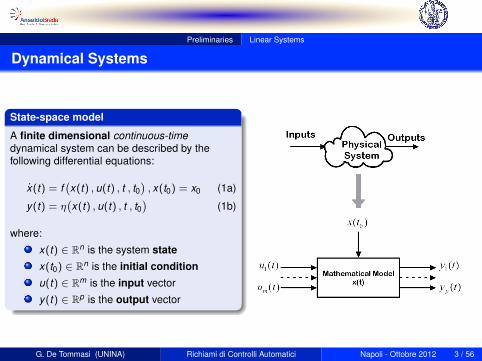
Preliminaries Linear Systems
Equilibria of nonlinear dynamical systems
Consider a nonlinear and time-invariant system
x(t) = f(x(t) ,u(t)
), x(0) = x0 (3a)
y(t) = η(x(t) ,u(t)
)(3b)
If the input is constant, i.e. u(t) = u, then the equilibriaxe1 , xe2 , . . . , xeq of such a system can be computed as solutions of thehomogeneous equation
f(xe , u) = 0 ,
Given an equilibrium xei the correspondent output is given by
yei = η(xei , u
).
G. De Tommasi (UNINA) Richiami di Controlli Automatici Napoli - Ottobre 2012 5 / 56
Preliminaries Linear Systems
Linearization around a given equilibrium
If x0 = xe + δx0 and u(t) = u + δu(t), with δx0 , δu(t) sufficientlysmall, then the behaviour of (3) around a given equilibrium
(u , xe
)is
well described by the linear system
δx(t) =∂f∂x
∣∣∣∣∣∣ x = xeu = u
δx(t) +∂f∂u
∣∣∣∣∣∣ x = xeu = u
δu(t) , δx(0) = δx0 (4a)
δy(t) =∂η
∂x∣∣∣∣∣∣ x = xe
u = u
δx(t) +∂η
∂u∣∣∣∣∣∣ x = xe
u = u
δu(t) (4b)
The total output can be computed as
y(t) = η(xe , u
)+ δy(t) .
G. De Tommasi (UNINA) Richiami di Controlli Automatici Napoli - Ottobre 2012 6 / 56
Preliminaries Linear Systems
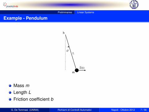
Example - Pendulum
Mass mLength LFriction coefficient b
G. De Tommasi (UNINA) Richiami di Controlli Automatici Napoli - Ottobre 2012 7 / 56
Preliminaries Linear Systems
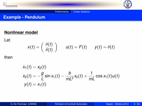
Example - Pendulum
Nonlinear model
Let
x(t) =
(θ(t)θ(t)
)u(t) = F (t) y(t) = θ(t)
then
x1(t) = x2(t)
x2(t) = −gL
sin x1(t)− bmL2 x2(t) +
1mL
cos x1(t)u(t)
y(t) = x1(t)
G. De Tommasi (UNINA) Richiami di Controlli Automatici Napoli - Ottobre 2012 8 / 56
Preliminaries Linear Systems
Example - Pendulum
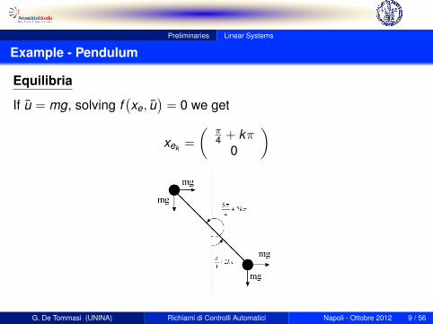
Equilibria
If u = mg, solving f(xe, u
)= 0 we get
xek =
(π4 + kπ
0
)
G. De Tommasi (UNINA) Richiami di Controlli Automatici Napoli - Ottobre 2012 9 / 56
Preliminaries Linear Systems
Example - Pendulum
Around the equilibria xe =(π4 0)T the behaviour of the pendulum is
well described by the linear system
δx1(t) = δx2(t)
δx2(t) = −√
2gL
δx1(t)− bmL2 δx2(t) +
1√2mL
δu(t)
δy(t) = δx1(t)
G. De Tommasi (UNINA) Richiami di Controlli Automatici Napoli - Ottobre 2012 10 / 56
Preliminaries Linear Systems
Asymptotic stability of LTI systems
Asymptotic stability
This property roughly asserts that every solution of x(t) = Ax(t) tends to zero as t →∞.
Note that for LTI systems the stability property is related to the system and not to a specificequilibrium.
Theorem - System (2) is asymptotically stable iff A is Hurwitz, that is if every eigenvalue λi ofA has strictly negative real part
<(λi)< 0 , ∀ λi .
Theorem - System (2) is unstable if A has at least one eigenvalue λ with strictly positive realpart, that is
∃ λ s.t. <(λ)> 0 .
Theorem - Suppose that A has all eigenvalues λi such that <(λi)≤ 0, then system (2) is
unstable if there is at least one eigenvalue λ such that <(λ)
= 0 which corresponds to a Jordan
block with size > 1.
G. De Tommasi (UNINA) Richiami di Controlli Automatici Napoli - Ottobre 2012 11 / 56
Preliminaries Linear Systems
Equilibrium stability for nonlinear systems
For nonlinear systems the stability property is related to the specificequilibrium.
Theorem - The equilibrium state xe corresponding to the constantinput u a nonlinear system (3) is asymptotically stable if all theeigenvalues of the correspondent linearized system (4) have strictlynegative real part.
Theorem - The equilibrium state xe corresponding to the constantinput u a nonlinear system (3) is unstable if there exists at least oneeigenvalue of the correspondent linearized system (4) which hasstrictly positive real part.
G. De Tommasi (UNINA) Richiami di Controlli Automatici Napoli - Ottobre 2012 12 / 56
Preliminaries Transfer function
Transfer function of LTI systems
Given a LTI system (2) the corresponding transfer matrix from u to y isdefined as
Y (s) = G(s)U(s) ,
with s ∈ C. U(s) and Y (s) are the Laplace transforms of u(t) and y(t)with zero initial condition (x(0) = 0), and
G(s) = C(sI − A
)−1B + D . (5)
For SISO system (5) is called transfer function and it is equal to theLaplace transform of the impulsive response of system (2) with zeroinitial condition.
Matlab commandssys = tf(num,den) creates a transfer function object.
G. De Tommasi (UNINA) Richiami di Controlli Automatici Napoli - Ottobre 2012 13 / 56
Preliminaries Transfer function
Transfer function
Given the transfer function G(s) and the Laplace transform of the inputU(s) the time response of the system can be computed as the inversetransform of G(s)U(s), without solving differential equations.
As an example, the step response of a system can be computed as:
y(t) = L−1[G(s)
1s
].
Matlab commands[y,t] = step(sys) computes the step response of the LTI systemsys.[y,t] = impulse(sys) computes the impulse response of the LTIsystem sys.
G. De Tommasi (UNINA) Richiami di Controlli Automatici Napoli - Ottobre 2012 14 / 56
Preliminaries Transfer function
Poles and zeros of SISO systems
Given a SISO LTI system , its transfer function is a rational function of s
G(s) =N(s)
D(s)= ρ
Πi(s − zi)
Πj(s − pj),
where N(s) and D(s) are polynomial in s, withdeg
(N(s)
)≤ deg
(D(s)
).
We callpj poles of G(s)zi zeros of G(s)
Matlab commandssys = zpk(z,p,k) creates a zeros-poles-gain object.p = eig(sys) or p = pole(sys) return the poles of the LTIsystem sys.z = zero(sys) returns the zeros of the LTI system sys.
G. De Tommasi (UNINA) Richiami di Controlli Automatici Napoli - Ottobre 2012 15 / 56
Preliminaries Transfer function
Poles and eigenvalues of a LTI system
Every pole of G(s) is an eigenvalue of the system matrix A. However,not every eigenvalue of A is a pole of G(s).
If all the poles of G(s) have strictly negative real part – i.e. they arelocated in the left half of the s-plane (LHP) – the SISO system is saidto be Bounded–Input Bounded–Output stable (BIBO).
A system is BIBO stable if every bounded input to the system results ina bounded output over the time interval [0,∞).
G. De Tommasi (UNINA) Richiami di Controlli Automatici Napoli - Ottobre 2012 16 / 56
Preliminaries Transfer function
Time constants, natural frequencies and damping factors
A transfer function can be also specified in terms oftime constants (τ ,T )natural frequencies (ωn,αn)damping factors (ξ,ζ)gain (µ)system type (i.e. number of poles/zeros in 0, g)
G(s) = µΠi(1 + Tis)Πj
(1 + 2 ζj
αnjs + s2
αnj
)sgΠk (1 + τks)Πl
(1 + 2 ξl
ωnls + s2
ωnl
) .
G. De Tommasi (UNINA) Richiami di Controlli Automatici Napoli - Ottobre 2012 17 / 56
Preliminaries Block diagrams
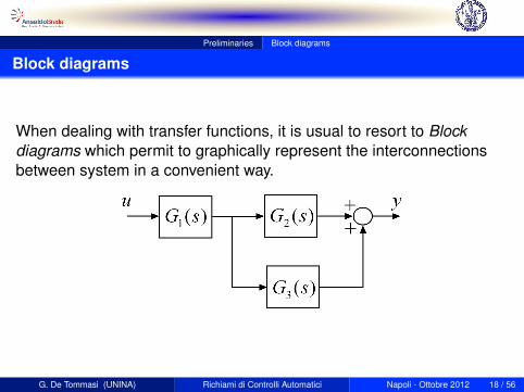
Block diagrams
When dealing with transfer functions, it is usual to resort to Blockdiagrams which permit to graphically represent the interconnectionsbetween system in a convenient way.
G. De Tommasi (UNINA) Richiami di Controlli Automatici Napoli - Ottobre 2012 18 / 56
Preliminaries Block diagrams
Series connection
Matlab commandssys = series(sys1,sys2) makes the series interconnectionbetween sys1 and sys2.
G. De Tommasi (UNINA) Richiami di Controlli Automatici Napoli - Ottobre 2012 19 / 56
Preliminaries Block diagrams
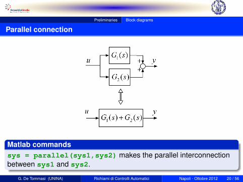
Parallel connection
Matlab commandssys = parallel(sys1,sys2) makes the parallel interconnectionbetween sys1 and sys2.
G. De Tommasi (UNINA) Richiami di Controlli Automatici Napoli - Ottobre 2012 20 / 56
Preliminaries Block diagrams
Feedback connection
Matlab commandssys = feedback(sys1,sys2,[+1]) makes the feedback interconnectionbetween sys1 and sys2. Negative feedback is the default. If the thirdparameter is equal to +1 positive feedback is applied.
G. De Tommasi (UNINA) Richiami di Controlli Automatici Napoli - Ottobre 2012 21 / 56
Preliminaries Block diagrams
Stability of interconnected systems
Given two asymptotically stable LTI systems G1(s) and G2(s)
the series connection G2(s)G1(s) is asymptotically stablethe parallel connection G1(s) + G2(s) is asymptotically stable
the feedback connection G1(s)1±G1(s)G2(s) is not necessarely stable
G. De Tommasi (UNINA) Richiami di Controlli Automatici Napoli - Ottobre 2012 22 / 56
Preliminaries Frequency response
Frequency response
Given a LTI system the complex function
G(jω) = C(jωI − A
)−1B + D ,
with ω ∈ R is called frequency response of the system.
G(jω) permits to evaluate the system steady-state response to asinusoidal input. In particular if
u(t) = A sin(ωt + ϕ) ,
then the steady-state response of a LTI system is given by
y(t) =∣∣G(jω)
∣∣A sin(ωt + ϕ+ ∠G(jω)
).
G. De Tommasi (UNINA) Richiami di Controlli Automatici Napoli - Ottobre 2012 23 / 56
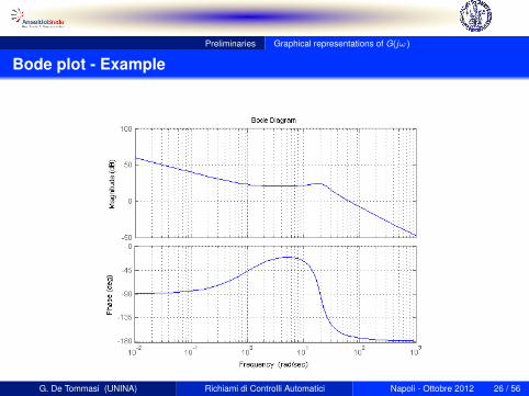
Preliminaries Graphical representations of G(jω)
Bode plot
Given a LTI system G(s) the Bode diagrams plotthe magnitude of G(jω) (in dB,
∣∣G(jω)∣∣dB = 20 log10
∣∣G(jω)∣∣)
and the phase of G(jω) (in degree)as a function of ω (in rad/s) in a semi-log scale (base 10).
Bode plots are used for both analysis and synthesis of controlsystems.
Matlab commandsbode(sys) plots the the Bode diagrams of the LTI system sys.bodemag(sys) plots the Bode magnitude diagram of the LTI systemsys.
G. De Tommasi (UNINA) Richiami di Controlli Automatici Napoli - Ottobre 2012 24 / 56
G. De Tommasi (UNINA) Richiami di Controlli Automatici Napoli - Ottobre 2012 25 / 56
Preliminaries Graphical representations of G(jω)
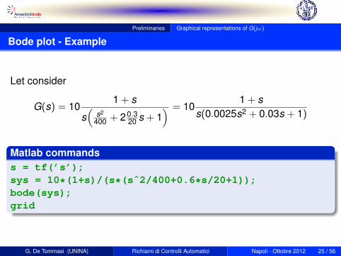
Bode plot - Example
G. De Tommasi (UNINA) Richiami di Controlli Automatici Napoli - Ottobre 2012 26 / 56
Preliminaries Graphical representations of G(jω)
Minimum phase systems
A stable system is said to be a minimum phase system if it has nottime delays or right-half plane (RHP) zeros.
For minimum phase systems there is a unique relationship betweenthe gain and phase of the frequency response G(jω). This may bequantified by the Bode’s gain-phase relationship
∠G(jω) =1π
∫ +∞
−∞
d ln |G(jω)|d lnω
ln∣∣∣∣ω + ω
ω − ω
∣∣∣∣dωω .
The name minimum phase refers to the fact that such a system has theminimum possible phase lag for the given magnitude response |G(jω)|.
G. De Tommasi (UNINA) Richiami di Controlli Automatici Napoli - Ottobre 2012 27 / 56
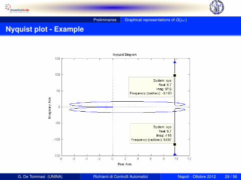
Preliminaries Graphical representations of G(jω)
Nyquist plot
The Nyquist is a polar plot of the frequency response G(jω) on thecomplex plane.
This plot combines the two Bode plots - magnitude and phase - on asingle graph, with frequency ω, which ranges in (−∞ ,+∞), as aparameter along the curve.
Nyquist plots are useful to check stability of closed-loop systems(see Nyquist stability criterion ).
Matlab commandsnyquist(sys) plots the Nyquist plot of the LTI system sys.
G. De Tommasi (UNINA) Richiami di Controlli Automatici Napoli - Ottobre 2012 28 / 56
Preliminaries Graphical representations of G(jω)
Nyquist plot - Example
G. De Tommasi (UNINA) Richiami di Controlli Automatici Napoli - Ottobre 2012 29 / 56
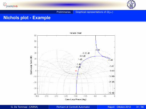
Preliminaries Graphical representations of G(jω)
Nichols plot
It is similar to the Nyquist plot, since it plots both the magnitude andthe phase of G(jω) on a single chart, with frequency ω as a parameteralong the curve.
As for the Bode plot the magnitude |G(jω)| is expressed in dB and thephase ∠G(jω) in degree.
Nichols charts are useful for the design of control systems, inparticular for the design of lead, lag, lead-lag compensators.
Matlab commandsnichols(sys) plots the Nichols chart of the LTI system sys.
G. De Tommasi (UNINA) Richiami di Controlli Automatici Napoli - Ottobre 2012 30 / 56
Preliminaries Graphical representations of G(jω)
Nichols plot - Example
G. De Tommasi (UNINA) Richiami di Controlli Automatici Napoli - Ottobre 2012 31 / 56
Feedback Control Systems The control problem
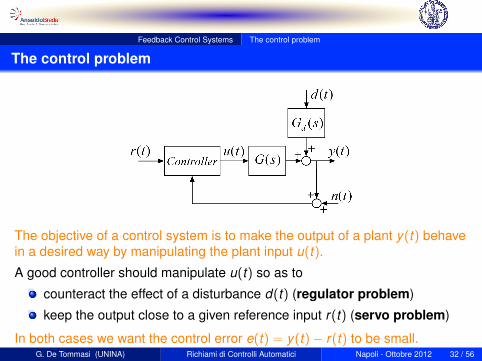
The control problem
The objective of a control system is to make the output of a plant y(t) behavein a desired way by manipulating the plant input u(t).
A good controller should manipulate u(t) so as to
counteract the effect of a disturbance d(t) (regulator problem)
keep the output close to a given reference input r(t) (servo problem)
In both cases we want the control error e(t) = y(t)− r(t) to be small.G. De Tommasi (UNINA) Richiami di Controlli Automatici Napoli - Ottobre 2012 32 / 56
Feedback Control Systems The control problem
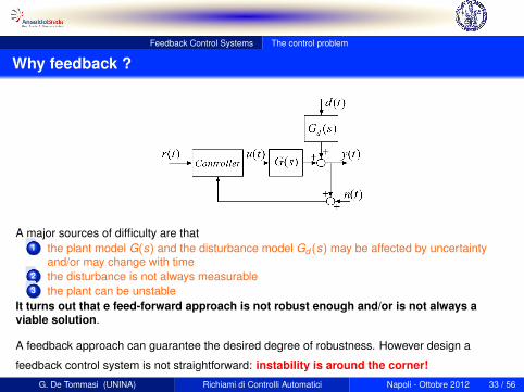
Why feedback ?
A major sources of difficulty are that1 the plant model G(s) and the disturbance model Gd (s) may be affected by uncertainty
and/or may change with time2 the disturbance is not always measurable3 the plant can be unstable
It turns out that e feed-forward approach is not robust enough and/or is not always aviable solution.
A feedback approach can guarantee the desired degree of robustness. However design a
feedback control system is not straightforward: instability is around the corner!
G. De Tommasi (UNINA) Richiami di Controlli Automatici Napoli - Ottobre 2012 33 / 56
Feedback Control Systems The control problem
Performance and stability
A good controller must guarantee:Nominal stability - The system is stable with no modeluncertaintyNominal Performance - The system satisfies the performancespecifications with no model uncertaintyRobust stability The system is stable for all perturbed plantsabout the nominal model up to the worst case model uncertaintyRobust performance The system satisfies the performancespecifications for all perturbed plants about the nominal model upto the worst case model uncertainty
G. De Tommasi (UNINA) Richiami di Controlli Automatici Napoli - Ottobre 2012 34 / 56
Feedback Control Systems The control problem
One degree-of-freedom controller
The input to the plant is given by
U(s) = K (s)(R(s)− Y (s)− N(s)
).
The objective of control is to manipulate design a controller K (s) suchthat the control error e(t) = r(t)− y(t) remains small in spite ofdisturbances d(t).
G. De Tommasi (UNINA) Richiami di Controlli Automatici Napoli - Ottobre 2012 35 / 56
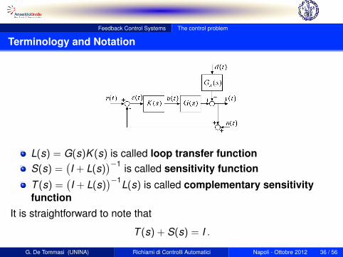
Feedback Control Systems The control problem
Terminology and Notation
L(s) = G(s)K (s) is called loop transfer functionS(s) =
(I + L(s)
)−1 is called sensitivity function
T (s) =(I + L(s)
)−1L(s) is called complementary sensitivityfunction
It is straightforward to note that
T (s) + S(s) = I .
G. De Tommasi (UNINA) Richiami di Controlli Automatici Napoli - Ottobre 2012 36 / 56
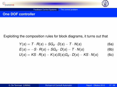
Feedback Control Systems The control problem
One DOF controller
Exploiting the composition rules for block diagrams, it turns out that
Y (s) = T · R(s) + SGd · D(s)− T · N(s) (6a)E(s) = −S · R(s) + SGd · D(s)− T · N(s) (6b)U(s) = KS · R(s)− K (s)S(s)Gd · D(s)− KS · N(s) (6c)
G. De Tommasi (UNINA) Richiami di Controlli Automatici Napoli - Ottobre 2012 37 / 56
Feedback Control Systems The control problem
One DOF controller
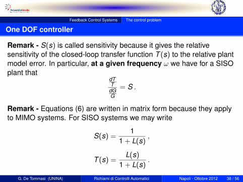
Remark - S(s) is called sensitivity because it gives the relativesensitivity of the closed-loop transfer function T (s) to the relative plantmodel error. In particular, at a given frequency ω we have for a SISOplant that
dTT
dGG
= S .
Remark - Equations (6) are written in matrix form because they applyto MIMO systems. For SISO systems we may write
S(s) =1
1 + L(s),
T (s) =L(s)
1 + L(s).
G. De Tommasi (UNINA) Richiami di Controlli Automatici Napoli - Ottobre 2012 38 / 56
Feedback Control Systems The control problem
The control dilemma
Let consider
Y (s) = T · R(s) + SGd · D(s)− T · N(s) .
In order to reduce the effect of the disturbance d(t) on the outputy(t), the sensitivity function S(s) should be made small(particularly in the low frequency range)In order to reduce the effect of the measurement noise n(t) on theoutput y(t), the complementary sensitivity function T (s) should bemade small (particularly in the high frequency range)
However, for all frequencies it is
T + S = I .
Thus a trade-off solution must be achieved.G. De Tommasi (UNINA) Richiami di Controlli Automatici Napoli - Ottobre 2012 39 / 56
Feedback Control Systems The control problem
Feedback may cause instability
One of the main issues in designing feedback controllers is stability.
If the feedback gain is too large then the controller may overreact and the closed-loop system
becomes unstable.
Download Simulink example
G. De Tommasi (UNINA) Richiami di Controlli Automatici Napoli - Ottobre 2012 40 / 56
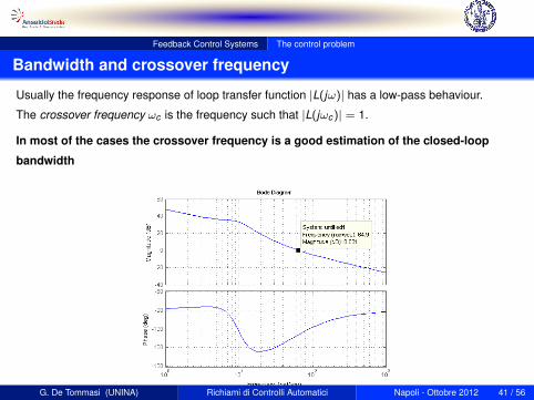
Usually the frequency response of loop transfer function |L(jω)| has a low-pass behaviour.
The crossover frequency ωc is the frequency such that |L(jωc)| = 1.
In most of the cases the crossover frequency is a good estimation of the closed-loop
bandwidth
G. De Tommasi (UNINA) Richiami di Controlli Automatici Napoli - Ottobre 2012 41 / 56
Feedback Control Systems Stability margins
Gain and phase margin
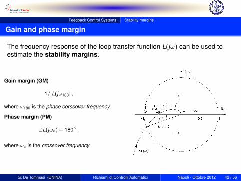
The frequency response of the loop transfer function L(jω) can be used toestimate the stability margins.
Gain margin (GM)
1/|L(jω180| ,
where ω180 is the phase corssover frequency.
Phase margin (PM)
∠L(jωc) + 180◦ ,
where ωc is the crossover frequency.
G. De Tommasi (UNINA) Richiami di Controlli Automatici Napoli - Ottobre 2012 42 / 56
Feedback Control Systems Stability margins
Gain Margin
The GM is the factor by which the loop gain |L(jω)| may be increasedbefore the closed-loop system becomes unstable.
The GM is thus a direct safeguard against steady-state gainuncertainty.
G. De Tommasi (UNINA) Richiami di Controlli Automatici Napoli - Ottobre 2012 43 / 56
Feedback Control Systems Stability margins
Phase Margin
The phase margin tells how much phase lag can added to L(s) atfrequency ωc before the phase at this frequency becomes 180◦ whichcorresponds to closed-loop instability (see Nyquist stability criterion ).
The PM is a direct safeguard against time delay uncertainty.
G. De Tommasi (UNINA) Richiami di Controlli Automatici Napoli - Ottobre 2012 44 / 56
Feedback Control Systems Nyquist Criterion
Nyquist Criterion - Preliminaries
The Nyquist Criterion permits to check the stability of a closed loopsystem by using the Nyquist plot of the loop frequency response L(jω).
The criterion is based on the fact the the close-loop poles are equal tothe zeros of the transfer function
D(s) = 1 + L(s) .
Hence, if D(s) has at least one zero z such that <(z) > 0 theclosed-loop system is unstable.
G. De Tommasi (UNINA) Richiami di Controlli Automatici Napoli - Ottobre 2012 45 / 56
Feedback Control Systems Nyquist Criterion
Nyquist Criterion
Consider a loop frequency response L(jω) and letP be the number of poles of L(s) with strictly positive real partZ be the number of zeros of L(s) with strictly positive real part
The Nyquist plot of L(jω) makes a number of encirclements N(clockwise) about the point (−1 , j0) equal to
N = Z − P .
It turns out that the closed-loop system is asymptotically if and only ifthe Nyquist plot of L(jω) encircle (counter clockwise) the point(−1 , j0) a number of times equal to P.
The criterion is valid if the Nyquist plot of L(jω) do not intersectthe point (−1 , j0).
G. De Tommasi (UNINA) Richiami di Controlli Automatici Napoli - Ottobre 2012 46 / 56
Feedback Control Systems Nyquist Criterion
Nyquist Criterion - Remarks
1 If the loop transfer function L(s) has a zero pole of multiplicity l ,then the Nyquist plot has a discontinuity at ω = 0. Further analysisindicates that the zero poles should be neglected, hence if thereare no other unstable poles, then the loop transfer function L(s)should be considered stable, i.e. P = 0.
2 If the loop transfer function L(s) is stable, then the closed-loopsystem is unstable for any encirclement (clockwise) of the point -1.
3 If the loop transfer function L(s) is unstable, then there must beone counter clockwise encirclement of -1 for each pole of L(s) inthe right-half of the complex plane.
4 If the Nyquist plot of L(jω) intersect the point (−1 , j0), thendeciding upon even the marginal stability of the system becomesdifficult and the only conclusion that can be drawn from the graphis that there exist zeros on the imaginary axis.
G. De Tommasi (UNINA) Richiami di Controlli Automatici Napoli - Ottobre 2012 47 / 56
Feedback Control Systems Root locus
Location of the poles of a closed-loop system
The time behaviour of a closed-loop system is strictly related to theposition of its poles on the complex plane.
For example, for a second order closed-loop system it is possible torelate the features of the step response such as
rise timeovershootsettling time
to the location of its poles.
The Root Locus design method permits to evaluate how changes in theloop transfer function L(s) affect the position of the closed-loop poles.
G. De Tommasi (UNINA) Richiami di Controlli Automatici Napoli - Ottobre 2012 48 / 56
Feedback Control Systems Root locus
The Root Locus
The closed-loop poles are given by the roots of
1 + L(s) . (7)
Assuming that L(s) = ρL′(s) the Root Locus plot the locus of allpossible roots of (7) as ρ varies in the range [0 ,∞).
The Root Locus can be used to study the effect of additional poles andzeros in L′(s), i.e. in the controller K (s).
The Root Locus can be effectively used to design SISO controllers.
Matlab commandsrlocus(sys) - plots the root locus for the loop transfer functionspecified by sys.
G. De Tommasi (UNINA) Richiami di Controlli Automatici Napoli - Ottobre 2012 49 / 56
Feedback Control Systems Root locus
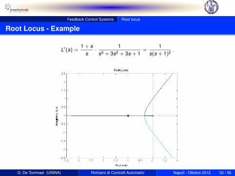
Root Locus - Example
L′(s) =1 + s
s·
1s3 + 3s2 + 3s + 1
=1
s(s + 1)2.
G. De Tommasi (UNINA) Richiami di Controlli Automatici Napoli - Ottobre 2012 50 / 56
Feedback Control Systems Root locus
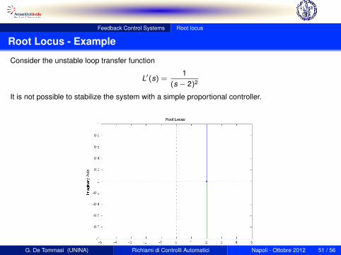
Root Locus - Example
Consider the unstable loop transfer function
L′(s) =1
(s − 2)2
It is not possible to stabilize the system with a simple proportional controller.
G. De Tommasi (UNINA) Richiami di Controlli Automatici Napoli - Ottobre 2012 51 / 56
Feedback Control Systems Root locus
Root Locus - Example
Add a pole in 0 to have zero steady-state error
L′(s) =1
s(s − 2)2
It is still not possible to stabilize the system with a simple proportional controller.
G. De Tommasi (UNINA) Richiami di Controlli Automatici Napoli - Ottobre 2012 52 / 56
Feedback Control Systems Root locus
Root Locus - Example
Add two zeros to draw the poles in the LHP
L′(s) =(s + 10)2
s(s − 2)2
The controller K (s) = ρ(s+10)2
s can stabilize the plant but is not causal.
G. De Tommasi (UNINA) Richiami di Controlli Automatici Napoli - Ottobre 2012 53 / 56
Feedback Control Systems Root locus
Root Locus - Example
Add an high frequency pole to have a proper controller
L′(s) =(s + 10)2
s(s + 100)(s − 2)2
The controller K (s) = ρ(s+10)2
s(s+100)can stabilize.
G. De Tommasi (UNINA) Richiami di Controlli Automatici Napoli - Ottobre 2012 54 / 56
Appendix
Suggested textbooks
P. Bolzern, R. Scattolini and N. SchiavoniFondamenti di Controlli AutomaticiMcGraw-Hill, 2008
R. C. Dorf and R. H. BishopControlli AutomaticiPearson Prentice Hall, 2010
G. F. Franklin, J. D. Powell and A. Emami-NaeiniFeedback Control of Dynamic SystemsPearson Prentice Hall, 2008
S. Skogestad and I. PostlethwaiteMultivariable Feedback Control - Analysis and DesignJohn Wiley and Sons, 2006
G. De Tommasi (UNINA) Richiami di Controlli Automatici Napoli - Ottobre 2012 55 / 56
Appendix
Feedback and Control for Everyone
P. Albertos, I. MareelsFeedback and Control forEveryoneSpringer, 2010
G. De Tommasi (UNINA) Richiami di Controlli Automatici Napoli - Ottobre 2012 56 / 56