RIEB Seminar, Kobe University,12 April 2012 Poverty ... · RIEB Seminar, Kobe University,12 April...

RIEB Seminar, Kobe University,12 April 2012

Poverty Dynamics of Households in Rural

China: Identifying Multiple Pathways for

Poverty Transition

Katsushi Imai

Economics, School of Social Sciences

University of Manchester

Jing You

School of Agricultural Economics and Rural Development

Renmin University of China RIEB Seminar, Kobe University 12 April 2012

2008 2010

Poverty Poverty

Poverty Non-Poverty

Non-Poverty Poverty

Non-Poverty Non-Poverty

(Ravallion, et al., 1995, JPE)

RIEB Seminar, Kobe University 12 April 2012

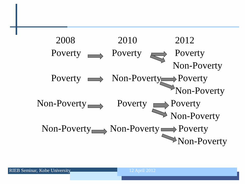
2008 2010 2012

Poverty Poverty Poverty

Non-Poverty

Poverty Non-Poverty Poverty

Non-Poverty

Non-Poverty Poverty Poverty

Non-Poverty

Non-Poverty Non-Poverty Poverty

Non-Poverty


Contents

1. Introduction

2. Methodology

3. Data

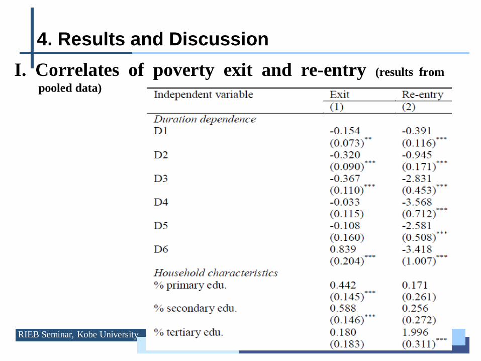
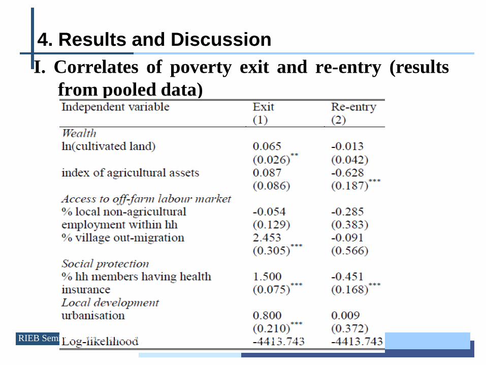
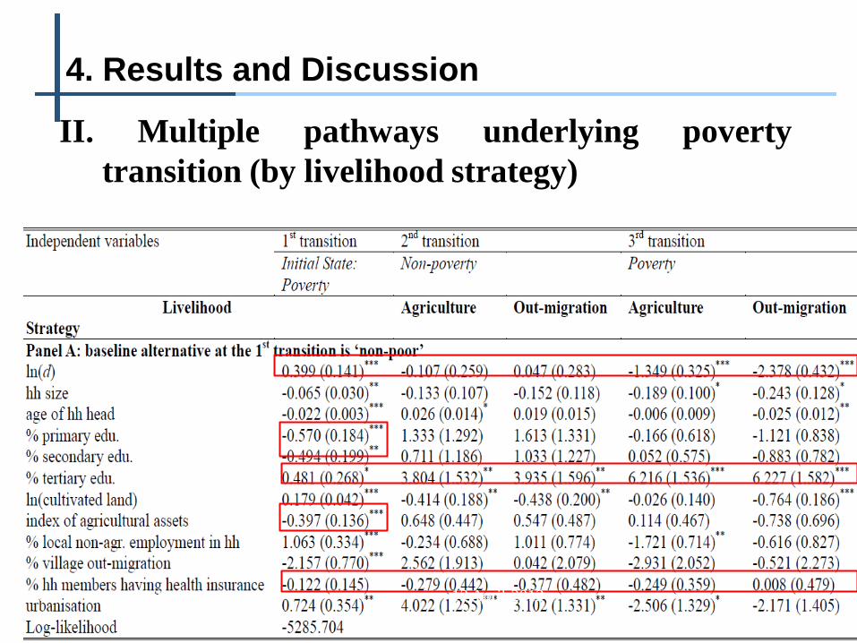
4. Results and Discussion

5. Conclusion


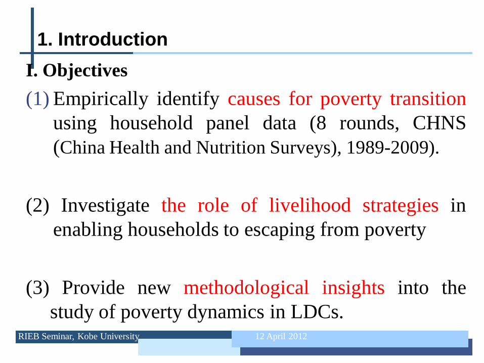
1. Introduction

I. Objectives

(1) Empirically identify causes for poverty transition

using household panel data (8 rounds, CHNS

(China Health and Nutrition Surveys), 1989-2009).

(2) Investigate the role of livelihood strategies in

enabling households to escaping from poverty

(3) Provide new methodological insights into the

study of poverty dynamics in LDCs. RIEB Seminar, Kobe University 12 April 2012

1. Introduction

II. Motivations

(1) Huge poverty reduction, but considerable mobility

in and out of poverty in LDCs and in China.

(e.g. Jalan and Ravallion 1998, 2000; Gustafsson and Sai, 2009).

Households are vulnerable- those who have become

non-poor are easy to slip back into poverty

(e.g. McCulloch and Calandrino, 2003, Imai et al., 2010).

……Evidence is scarce


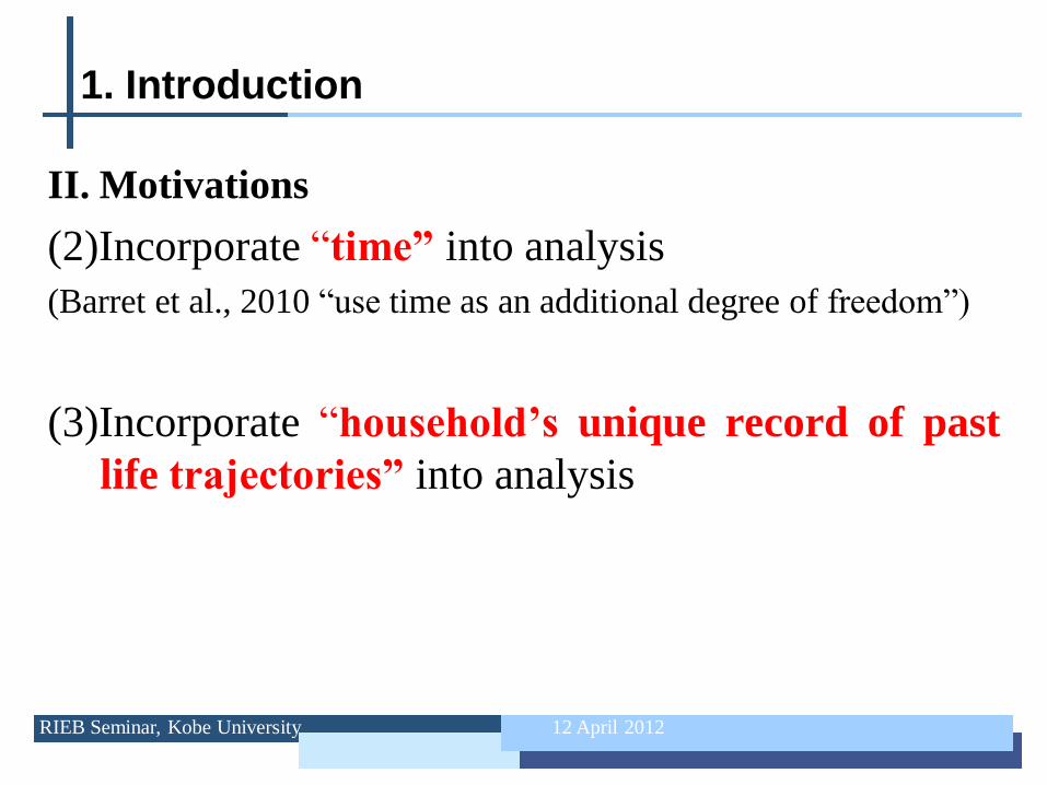
1. Introduction

II. Motivations

(2)Incorporate “time” into analysis

(Barret et al., 2010 “use time as an additional degree of freedom”)

(3)Incorporate “household’s unique record of past

life trajectories” into analysis


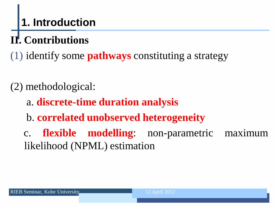
1. Introduction

II. Contributions

(1) identify some pathways constituting a strategy

(2) methodological:

a. discrete-time duration analysis

b. correlated unobserved heterogeneity

c. flexible modelling: non-parametric maximum

likelihood (NPML) estimation


2. Methodology for ‘Poverty Dynamics’ studies

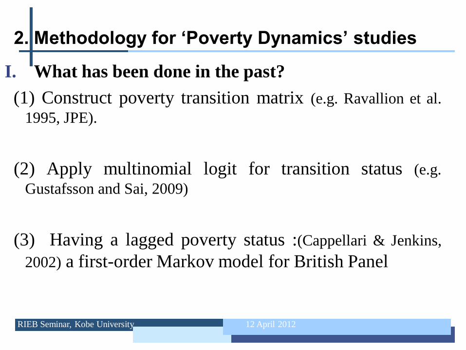
I. What has been done in the past?

(1) Construct poverty transition matrix (e.g. Ravallion et al.

1995, JPE).

(2) Apply multinomial logit for transition status (e.g.

Gustafsson and Sai, 2009)

(3) Having a lagged poverty status :(Cappellari & Jenkins,

2002) a first-order Markov model for British Panel


2. Methodology for ‘Poverty Dynamics’ studies

(4) Applying duration analysis

*Developed countries: Canto(2002) for Spain, Devicienti (2002,

11) for Britain; Maes (2011) for Belgium.

*LDCs: Baulch and McCuuloch (2002): Assumed continuous

data for discrete data (Pakistan).

Bigsten and Shimeles (2008) Discrete hazards (Ethiopia)

Glauben et al. (2006): continuous data assumed (only

Zhejiang).

Limitations: (1) Unobserved heterogeneity ignored. (2)

Dynamic selection / past history ignored. (3) Initial

endogeneity ignored.


2. Methodology

empirical specification (complementary log-log)

(e.g. Devicienti, 2002).

• hazard rate of exit (the probability that household i

escapes from poverty at duration d at time tj

•

• :

, | 1 exp expP P P P

i ij i ij ie d X f d X u

fP(d) : the baseline hazard which is a function of duration that i has been

stuck in poverty spells

Xij : household-specific characteristics and aggregate covariates;

P

i

P

iu log : the unobserved household-specific heterogeneity which

is time-invariant. RIEB Seminar, Kobe University 12 April 2012

2. Methodology

• hazard rate of re-entry:

• baseline hazard: 3 different specifications;

, | 1 exp expN N N N

i ij i ij ir d X f d X u

(1) a parametric specification: fP(d)=ln(d) and f

N(d)=ln(d);

(2) 3 time-period dummies, each of which containing two durations;

(3) a non-parametric form, that is, a set of ‘duration-interval’ specific

dummies at which households are at risk of shifting out of (non-)

poverty spells.


2. Methodology

• unobservables: 2 different ways of modelling

• Here we only report the results of the most

flexible one based on Heckman & Singer

(1984)or Karlson (2011) using NPML.

(1) Parametric: normal and gamma distributions are assumed for the

unobserved heterogeneity in turn

(2) Non-parametric: Heckman and Singer’s (1984) non-parametric

maximum likelihood (NPML) estimation where the distribution of

unobserved heterogeneity is approximated by a bivariate discrete

distribution with a number of latent classes – also termed as mass

points – which are left determined by the data.


2. Methodology

Heckman & Singer’s (1984) NPML for correlated

unobservables

• groups of households with different

unobservables in exit

• groups of households with different

unobservables in re-entry

• hazard rate of exit:

• hazard rate of re-entry:

• the joint distribution of correlated unobservables:

, | 1 exp expP P P P

i ij i ij we d X f d X

, | 1 exp expN N N N

i ij i ij wr d X f d X

1,2, ,w W

1 1, , , , ,P P N P

W WG

1,2, , 'w W


2. Methodology

III. Modelling multi-path of multiple poverty transitions

(panel data) (‘dynamic selection’ model)

“putting time on the map” of poverty analysis (Clark and

Hulme, 2010, p.352)

We focus on: (i) multiple spells of poverty and non-poverty,

(ii) endogenous ‘dynamic selection’ (Cameron & Heckman,

1998).

(iii) unobserved heterogeneity correlated across spells as well

as various destinations within the spell.

“A choice of pathways” is guided by a simpler version of

duration models.


2. Methodology

III. Modelling multi-path of multiple poverty

transitions (panel data) (‘dynamic selection’ model)

(1) By Livelihood Strategy


2. Methodology

II. Modelling multi-path of multiple poverty

transitions (panel data)

(2) Multinomial transition model with unobserved

heterogeneity (MTMU, Karlson, 2011)

Issues in modelling:

• at each transition, correlated unobservables across

destinations: inter-dependent livelihood options

• over multiple transitions, correlated unobservables

across transitions: dynamic selection (which also

takes account of “endogenously initial status”).


2. Methodology

II. Modelling multi-path of multiple poverty

transitions (panel data)

(2) By Health Insurance (Gustafsson and Li, 2004, CER)


3. Data

China Health and Nutrition Surveys (CHNS), 1989-2009 (8

rounds) 1,304 rural households in 7 provinces.


3. Data

(a) Advantage:

Long balanced panel data

Disadvantage: non-random attrition- but not so large.

[24.5% of households reported ‘excluded’ family members; in one

of the eight survey years. For these households, the average

number of ‘excluded’ family members was around only 1.5.]

New household members: very rare.

(b) 7 provinces; Jiangsu, Shandong, Henan, Hubei, Hunan,

Guangxi and Guizhou (Liaoning and Heilongjiang, are

excluded because of missing observations).


3. Data

(c) We use consumption to measure poverty.

-Use the international poverty lines of US$1.25/day and US$2/day.

-Follow Devicienti (2002) and define the poor as those whose per

capita household consumption falls below 90% (or 110%) of the

recalculated poverty lines of US$1.25/day and US$2/day

(‘adjusted’ poverty lines).

-Also use a food poverty line of 620 yuan in 2002 prices based on

2,100 calories intake per person per day to check the robustness of

poverty statistics.


3. Data

Fig. 2 Profile of poverty rates


3. Data

Fig. 3 Distribution of the number of transitions (spells)


3. Data


Fig. 4 Distribution of the length of poverty spells


I. Correlates of poverty exit and re-entry (results from

pooled data)



I. Correlates of poverty exit and re-entry (results

from pooled data)



I. Correlates of poverty exit and re-entry (results

from pooled data) Independent variable Poverty

Exit

Poverty

Re-Entry

(2) (5)

Social protection

% hh members having commercial

insur.

-0.641

(0.241)***

-0.040

(0.798)

% hh members having government

free insur.

-0.313

(0.302)

0.119

(0.639)

% hh members having cooperative

insur.

[NCMS (National Cooperative

Medical Scheme)]

1.515

(0.075)***

-0.542

(0.206)***



Other factors that promotes poverty exit:

-smaller hh size; -older hh head;

-larger cultivated land

-urbanisation index (econ. activities, inc. marketisation;

infrastructure, communication) Jones-Smith & Popkin

Other factors that prevents poverty reentry:

-agricultural asset accumulation

Role of agriculture in poverty reduction

[Christiansen et al., 2011; de Janvry and Sadoulet 2010-

agricultural productivity matters]



Independent variable Poverty

Exit

Poverty

Re-Entry

(3) (6)

economic activity -0.011

(0.011)

-0.023

(0.023)

access to markets 0.026

(0.008)***

0.001

(0.014)

social service

(provisions of

preschool)

0.054

(0.013)***

0.019

(0.038)



II. Multiple pathways underlying poverty

transition (by livelihood strategy)


(1) By Livelihood Strategy



II. Multiple pathways underlying poverty transition

(by social protection)


(2) By Health Insurance (Gustafsson and Li, 2004, CER)


5. Conclusions

(1) The likelihood of exiting poverty first decreases and

then increases as households have spent more time in

poverty. The longer the households have stayed above

the poverty line, the lower chance of re-entry into

poverty.

(2) However, agriculture or out-migration helped poverty

exit (but outmigration mainly for the initially non-poor).

(3) Primary and secondary education helped poverty exit.


5. Conclusions

(4) Cultivated land matters for reducing initial poverty and

prevents poverty re-entry (for those out-migrated).

Agricultural assets served as reducing initial poverty.

(5) Health insurance matters, but is not universally good (it

effect depends on the path of livelihood strategies). –


5. Conclusions

(7) Policy should;

(a) pay attention to dynamic aspects of poverty.

take different stages of transitions into account (e.g.,

education, urbanisation);

(b) needs to support the chronically poor;

(c) agriculture matters (cultivated land; agricultural land

to help the poor escape from poverty; safety-nets).

(d) Cooperative insurance (NCMS) was effective in

helping the poor escape from poverty and prevent the

poor from backsliding.


Thank You!

Q&A


Date post:	17-Apr-2018
Category:	Documents
Upload:	nguyenthuan
View:	214 times
Download:	2 times

RIEB Seminar, Kobe University,12 April 2012 Poverty ... · RIEB Seminar, Kobe University,12 April...

Documents