Rijksinstituut voor Kust en Zee - RIKZ

WL | delft hydraulics

Benchmarking database for Delft3D

November, 2006

Z4099

Report

Rijksinstituut voor Kust en Zee - RIKZ

Prepared for:

Prepared for:

Benchmarking database for Delft3D

D.J.R. Walstra and L. Koster

Report

November, 2006

Benchmarking database for Delft3D Z4099 November, 2006

WL | Delft Hydraulics i

Contents

1 Introduction .................................................................................................... 1—1

1.1 General ................................................................................................ 1—1

1.2 Testbank objectives .............................................................................. 1—1

1.3 Readers guide ...................................................................................... 1—2

2 Benchmarking database for Delft3D.............................................................. 2—1

2.1 Introduction ......................................................................................... 2—1

2.2 Data sets .............................................................................................. 2—1

2.3 Structure .............................................................................................. 2—2

2.3.1 Case directories ....................................................................... 2—3

2.3.2 Model directories..................................................................... 2—3

2.3.3 Entering new dataset in database..............................................2—4

3 Benchmarking datasets: 1. Laboratory measurements ................................. 3—1

3.1 Overview ............................................................................................. 3—1

3.2 Arcilla et al. (1994), Roelvink and Reniers (1995) ................................ 3—1

3.2.1 Dataset description .................................................................. 3—1

3.2.2 Model setup............................................................................. 3—2

3.2.3 Results .................................................................................... 3—3

3.3 Reniers et al. (1997) ............................................................................. 3—3


3.4 Boers (1996) ........................................................................................ 3—4


3.5 H4357 Dune erosion ............................................................................ 3—5



WL | Delft Hydraulics i i

4 Benchmarking data sets: 2. Field measurements........................................... 4—1

4.1.1 Overview................................................................................. 4—1

4.2 Sand-ridge (Tonnon, 2005)................................................................... 4—1

4.2.1 Data set description ................................................................. 4—1

4.2.2 Cases and model set-up............................................................ 4—2

4.2.3 Results .................................................................................... 4—4

4.3 Grays Harbor (Walstra et al., 2005) ...................................................... 4—4



4.4 Duck (1994)......................................................................................... 4—7


4.4.2 Model set-up ........................................................................... 4—8

4.5 Egmond Hydrodynamic ....................................................................... 4—8



4.6 Egmond Morphodynamic................................................................... 4—10

4.6.1 Cases..................................................................................... 4—10

4.6.2 Measurements ....................................................................... 4—10

4.6.3 Reference model.................................................................... 4—10

4.7 EgmondLong ..................................................................................... 4—10

4.7.1 Dataset description ................................................................ 4—10

4.7.2 Model setup........................................................................... 4—10

5 Statistical analysis ........................................................................................... 5—1

5.1 Statistical tool ...................................................................................... 5—1

5.2 Model performance statistics ................................................................ 5—1

5.3 Practical Example ................................................................................ 5—3


WL | Delft Hydraulics i i i

6 Recommendations........................................................................................... 6—1

6.1 Application of the testbank................................................................... 6—1

6.2 Data sets .............................................................................................. 6—1

7 References .......................................................................................................7—1

A Benchmarking – Tool....................................................................................... A–1

A.1 Making new models .............................................................................. A–1

A.2 Comparing and analysing model results................................................. A–2

B Egmond Coast3D............................................................................................. B–1

B.1 Measurements and instrumentation........................................................ B–1


WL | Delft Hydraulics 1 — 1

1 Introduction

1.1 General

This report describes the progress made of the short term morphology project with thecollaborative research agreement between WL | Delft Hydraulics and RIKZ (VOP)concerning the Delft3D Testbank. This report focuses on the structural improvements madeto the Delft3D testbank (adding cases, improving pre- and post-processing tools). Besides ofthat a description of the included datasets, processing tools and how to use the testbank isprovided.

The testbanks primary purpose is to facilitate testing and validation activities using theDelft3D model. It provides ready made input files, pre- and postprocessing facilities whichcan consistently be applied for all (or a selection) of the available test cases. The testbank isdesigned for experienced modellers developing and improving Delft3D. To ensureflexibility, low level matlab scripts are available which require a basic understanding ofMatlab. Furthemore no precautions have been with respect to applying unrealistic modelsettings.

Although the testbank is primarily designed for internal use at WL | Delft Hydraulics,external users can use the testbank freely. The testbank has an open structure which allowsfor an easy extension of the datasets or modification of data or input files. The testbankcould even be used in combination with other models. However, this requires a modificationof the pre- and postprocessing scripts.

This report provides a comprehensive description of the structure of the testbank, datasets,and pre- and postprocessing facilities. It is highly recommended to read this report inconjunction with the testbank itself installed.

1.2 Testbank objectives

Numerical models have become one of the corner stones of coastal engineering and areoften applied tools to obtain answers or solutions for a specific coastal question or problem.Essential phases in a proper modelling framework are calibration and validation. Calibrationinvolves model parameter tuning such that optimum agreement with measurements isobtained. During the validation no optimisation of model performance is allowed becausethe model with settings obtained during calibration is tested on other data. This gives anindication of the model’s predictive capabilities for the problem under consideration.

Until recently, various model settings and model versions were calibrated and validated ondifferent data sets, thereby obscuring model performance in general. To overcome this, adatabase with existing laboratory and field data sets was constructed for the process-basedmorphological model UNIBEST-TC (Roelvink et al., 2000) with the aim to:

integrate model and measurements,



facilitate easy testing of model settings and versions against a wide range of conditions,andidentify shortcomings in understanding of physical processes, both considering modelformulations and measurements.

The past years the Testbank has proven to be a valuable instrument to store datasets, sharethem amongst modellers and validate profile models. Due to the continuous development ofDelft3D, many of the relevant cross-shore processes have been implemented. The presentversion of Delft3D has all the functionality of a profile model (such as Unibest-TC). Thishas resulted in a gradual decrease of the Unibest-TC applications whereas the application ofDelft3D has increased. Therefore it was necessary to upgrade the existing Delft3D testbankwith the relevant cases from the Unibest-TC testbank.

Another development has been the increased use of Matlab and its links with Delft3D. In theoriginal Testbank fortran-based programs were used e.g. for data extraction, and erroranalysis, only for the graphical post-processing Matlab was used. In the upgrade describedin this report all data processing has been migrated to the Matlab environment.

This report describes the updated database structure, the various implemented data sets andan example on how the database can be used with different model settings.

The new testbank has been improved on the following topics:Facilitating an easy way to prepare new models based on a certain basis setting andtesting (a set of) different models settings (e.g. enhanced modification of input files);Analysing different combinations of model results by plotting them againstmeasurements and showing the effect of different parameters (improved post processingand visualisation tools);Performing a statistical analyses on model and measured data to give a quantitative ideaof the performance (statistical analysis now based on Matlab scripts);Creating Delft3D-input file for a number of experiments.

1.3 Readers guide

Chapter 2: Benchmarking database for Delft3DThis chapter describes the data base structure and outlines how a new data set can beimplemented.

Chapter 3: Benchmarking data sets: I. Laboratory measurementsHere, the implemented laboratory data sets are discussed. The set-up of the cases and runsincluded per data is described. For this particular project, a ‘basic’ model version has beendeveloped.

Chapter 4: Benchmarking data sets: 2. Field measurementsThis chapter is devoted to a description of the implemented field data sets and thecorresponding model-data comparison.



Chapter 5: Statistical analysisThe database is accompanied by a Statistical Analysis Tool which allows quantifying model-data differences. With model performance statistics the effect of the improvement orreduction in model skill for different model settings can be easily quantified. Chapter 5provides an example on the use of SAT.

Finally a list of conclusions for the reference performance of Delft3D and a list ofrecommendations for further research are provided in Chapter 7.



2 Benchmarking database for Delft3D

2.1 Introduction

The benchmarking database of Delft3D is intended to include datasets of various tests (fieldand laboratory) against which the model can be tested automatically for a wide range ofsettings. In this stage only data sets for profile models are included to compute cross-shoresediment transport and the resulting profile changes along a coastal profile of arbitraryshape under wave attack. Variation in wave- and tide-induced longshore transport rates canalso be accounted for. Main applications are the simulation of sand bar dynamics andseasonal profile changes, as well as the design of beach nourishment schemes. The datasetsthat will be incorporated in the database should enable a complete qualification of theaccuracy of the description of the implemented physical processes and the accuracy andreliability of the final results: the computed longshore sediment transport and the predictedprofile development.

The installation of the database (provided on the CD-ROM) involves a simple copying ofthe entire contents of the CD-ROM to the desired directory on a PC. Because running themodel will produce new files, sufficient hard-disk space should be available. The databasecannot be run from the CD-ROM itself or from a network drive for which the database userhas no write-permission. Furthermore, it is necessary to have Matlab installed.

2.2 Data sets

The testbank contains a set of nine tests of which five of them are taken from the originaldatabase, four new cases are added:

Table 2.1 Overview of available datasets.

Laboratory measurements Field measurements

Boers

Lip11d-hydr

Lip11d-morph

Reniers

H4357

Egmond / Coast3D

Duck94, US

Sand-ridge

Grays Harbor, US

From Table 2.1 five data sets were part of the Unibest TC database and were converted toDelft3D models. Four new datsets were added in the present database, the H4357 duneerosion experiment and field experiments from Grays Harbor, Duck94 and the sand-ridge.The various data will be discussed more detailed in chapter 3 and 4.



The datesets mentioned so far are all cases with only 1 horizontal dimension (cross-shore ortransect models). If other interesting datasets become available these can easily be included.

2.3 Structure

The database structure is similar to that of the Unibest-TC database (Roelvink et al., 2000)and mainly consists of three levels:

1. The primary level contains various test directories and the executable for theBenchmarking Tool;

The benchmarking tool is a Matlab based tool providing a simple way to work with thedatabase. The objective is to facilitate a method for creating new models and analysingmodel results without having to enter all directories. With a simple double-click on thetestbank-executable “testbank.bat”, Matlab will guide the user through a number ofpossibilities. The matlab scripts are all stored in a directory named ‘work’, which is locatedat the level of the test-directories so copying of the full database will include access to thetool. For a more elaborated description, see Appendix A.

2. Within a test directory different case directories are present. The different cases are forexample different initial bathymetries or different boundary (test) conditions. The casedirectories contain measured data and various Delft3D model directories. At this levelan analysis directory is created as soon as the first plots are stored with thebenchmarking tool.

3. The model directories contain the different models and its output in the form of thestandard output together with the formatted output files created by the tool.

test-dir case-dir model-dir

lip11d-hydr 1a v1

gamdis05

Figure 2-1 Database structure



Figure 2-1 illustrates the structure of the database. Test Lip11d-hydr contains 7 cases(1a,1b,1c,2a,2b,2c and 2e). Case 1a contains two Delft3D models: v1 and gamdis which arebased on the basis model located on the same level. Different plots and text files are storedin the analysis directory.

2.3.1 Case directories

The case directory contains the measured data on which the models are calibrated. Thesedata are stored in a simple TEKAL-format, each containing only one physical parameter.The TEKAL-format comprises one data block with two columns. The first column is a timeor space vector and the second is the measured parameter e.g. hrms or depth. The file namesare standardised, which is necessary for the tool to recognise them and for furtherprocessing of the Delft3D output. The general layout of the names is as follows:

parameter distribution descriptionrtfX065 f(z) Return flow profilesconcX065 f(z) Concentration profilesdepth f(x) Profile depthhrms f(x) Root mean square wave heighteta f(x) Water levelstotx f(x) Total transport in x-directionuymean f(x) Mean velocity in y-directionzt0001 f(x) Profile depth at timeztyear1997 f(x) Profile depth in year

<param> .tek time and location independent<param>Xxxx.tek at location x, time independent<param>Ttttt.tek at time t, location independent

2.3.2 Model directories

The basis directories contain the model files needed to run Delft3D (initial conditions,boundary conditions, parameters grids etc.). With the benchmarking tool new models can becreated with a basis setting as reference. After running the model Delft3D output can beprocessed and the model data (results) are written to the described TEKAL-formats. Namesof measured data- and model data-files are identical but on two different levels, making iteasy to compare results.

Profile modelling

The modelling system applied in this study is the Sediment Online version of Delft3D,which is described in detail in Lesser et al. (2004). A crucial extension to the Delft3D-FLOW model, for coastal applications, is the capability to allow for alongshore water levelgradients to be applied at lateral model boundaries (Roelvink and Walstra, 2004). To makethe solution well posed a water level boundary is required at the seaward model boundary.Roelvink et al. (2004) demonstrated that applying Neumann boundary conditions allowedfor reliable predictions to be made when using only one grid cell in the alongshore direction



(i.e. effectively reducing a 2DH/3D model to a 1DH/2DV model) under the combinedforcing of (breaking) waves, wind and tide.

All profile models are run in 2DV mode with a varying horizontal grid resolution. Thevertical grid consists of -layers with an increased resolution near the bed and water surfaceto accurately account for hydrodynamic and sedimentological phenomena (e.g. turbulenceproduction due to breaking waves, streaming near the bed, and suspended sedimenttransport) in the flow equations and the associated turbulence model (k- , Walstra et al.,2000). The roller model is used to obtain an accurate cross-shore wave forcing distribution.Snell’s Law (implemented in Flow module) provides the wave direction across the profile.The state-of-the-art transport formulations of TR2004 (Van Rijn et al., 2004) including bedroughness predictors were applied to estimate transport rates and bed evolution. All modelsettings are initially set to default values.

2.3.3 Entering new dataset in database

The database has a very straight and clear structure in which model data and measurementdata are stored at different levels. To ensure that the benchmarking-tool can be run, thisstructure should be preserved. Installation of the database involves copying of the entiredatabase to a local disk after which running of the tool is possible. Together with thedatabase Matlab and Delft3D are necessary. For successful usage of the database a numberof steps have to be taken in case of entering a new dataset:

Making a new test directory at highest level <test-dataset>;Dividing the test directory in cases. If only one case is tested a case directory has to bemade as well <case>;Filling the case-dir with measured data in the described format of TEKAL-files;Making a basis Delft3D model with the directory-name ‘basis’. The batch file must benamed run1.bat <model>If the entering of the new dataset is finished successful, testing and analysing can begin.



3 Benchmarking datasets: 1. Laboratorymeasurements

3.1 Overview

In Table 3.1 an overview is given of the implemented laboratory measurements. Adescription of each data set and of the model-data comparison is provided in Sections 3.2 -3.5.

Table 3.1 Overview of laboratory data sets and parameters

Code Waves andset-up

Current(2DV)

Current(3D)

Concen-trations andtransport

Bottomchange

Dune ErosionDelta Flume

H4357 * * * * z (x,t)

Arcilla et al. (1994)Delta Flume

LIP11D HrmsEta

u(z)urmsguss, guls

c(z)Stotx

z (x,t)

Reniers et al. (1997) Reniers HrmsEta

u,vurms

Boers(1996)

Boers HrmsEta

u(z)urmsguss, guls

Hrms = root-mean-square wave heightEta = set-up/downu, v = cross-shore and longshore velocityz = vertical (i.e., vertical profiles are available)urms = root-mean-square cross-shore velocityguss = short-wave velocity momentguls = short-wave long-wave interaction velocity momentc = sediment concentrationStotx = total cross-shore sediment transport*) = will be added later if data becomes available (expected early 2007).

3.2 Arcilla et al. (1994), Roelvink and Reniers (1995)

3.2.1 Dataset description

Arcilla et al. (1994) conducted a series of comprehensive morphological tests in the large-scale Delta Flume at Delft Hydraulics. Seven tests were carried out in two series. The firstseries, tests 1a, 1b and 1c, were carried out from an initial Dean-type profile, with a mildlysloping dry beach; the second series was carried out starting from an initial profile with adune at the waterline but the same underwater profile. Extensive measurements were carriedout of wave heights, water levels, flow profiles, wave asymmetry and long waves,concentration profiles and bottom changes. The latter were used to derive total transport



rates. Each test lasted 12 to 21 hrs and measurements were carried out throughout everywave hour.

The incident wave height, wave period, water level and sub-test duration for the differentsub-tests are presented in Table 3.2.

Table 3.2 Test conditions for Arcilla et al. (1994)

Test code Initial geometry Hmo (m) Tp (s) water level (m) Duration (h)

1a Dean-type 0.9 5 4.1 12

1b result of 1a 1.4 5 4.1 18

1c result of 1b 0.6 8 4.1 13

2a Dean-type with dune 0.9 5 4.1 12

2b result of 2a 1.4 5 4.1 12

2e result of 2b 1.4 5 4.6 18

2c result of 2e 0.6 8 4.1 21

As the table shows the final profiles of test 1a and 1b are applied as initial profile for test 1band 1c. The same is true for case 2 wherein the sequence is some different. The figure showsthe initial profiles of the first and the last tests within the two cases.

Figure 3-1 Initial profiles (solid) and final profiles (dots) for test 1 and 2

3.2.2 Model setup

In order to reduce the number of morphodynamic cases, the morphological andhydrodynamic results have been split over two datasets with different models, lip11d-hydrand lip11d-morf. Each hydrodynamic test was carried out for one profile somewhere in themiddle (near 6 wave hours). Although not all data were collected at the same time thisdiscrepancy was not too severe. Rather than carrying out complete morphological runs thesediment transports derived from the measured bed level changes is compared with thecomputed total transport rates. This reduces the data set to 7 cases.



3.2.3 Results

To show the functionality of the database in combination with the tool, an example is givenfor the standard model together with two variations on the gamma-expression (wave heightto water depth ratio for breaking waves). In appendix 3.2 the results are plotted for both thehydrodynamic as the morphodynamic models with the following variation:

Table 3.3 Parameter settings for different model runs

Name Parameter Value

v1 (basis settings) gamdis ruessink et al. (2002)

gamdis05 gamdis 0.5

gamdis07 gamdis 0.7

In chapter 5 some more sensitivity testing is done and the performance has been analysed ina more quantitative, statistic way.

Hydrodynamics

Figure 3.2.1 shows the vertical velocity profile in cross-shore direction. Best predictions areseen for gamma =0.7 and Ruessink et al. (2002). However different locations show differentresults. Especially on deeper water little agreement is seen. Apparently calibration of themodel is needed to get better results on sediment transports. Fig. 3.2.3 shows results onwave height and water level elevation. The effect of the gamma – expression is most clearfor the wave heights. The lower plot shows the total sediment transport in x direction.

Morphodynamics

In case of bottom updating, Appendix 3.2.4, it is seen that different gamma-expression doesnot give large variation on the cross-shore profile. Overall the agreement with themeasurements is good. For the gamma =0.7 and Ruessink et al. (2002) situations barforming is seen at shallow water. The Ruessink expression shows the best results.

3.3 Reniers et al. (1997)


This dataset refers to experiments in the multi-directional wave basin at Delft Hydraulics,aimed at the study of shear instabilities of the longshore current. For this purpose, a barredbeach was constructed at an angle of 30 degrees with respect to the wave paddles. Thewave-generated longshore current was recirculated using a pump system and a carefullayout of the inflow and outflow sections, resulting in quite uniform mean flow conditions.Most of the tests were carried out with regular waves, except for case SO014, which wasdone with random, unidirectional waves. The latter case has been included in the database.



Table 3.4 Test conditions for Reniers et al., (1997)

Test code Hs (m) Tp (s) water level (m)

SO014 0.1 1.2 0.55

Figure 3-2 Profile Reniers et al. (1997), test SO014

3.4 Boers (1996)


This is an extremely detailed, high-quality set of hydrodynamic data in a wave flume atDelft University. This fixed-bed dataset is a reproduction of the mobile-bed dataset ofLIP11D, allowing much more detailed study of the hydrodynamic parameters. Only aselection of the full dataset has been chosen for comparison with Delft3D:

Hrms wave heightEta, wave setupRTFX, vertical profiles of the time-averaged horizontal velocityC, wave celerity across profileGuls, guss, velocity moments.Q, fraction of breaking waves (derived from video images)

Table 3.5 shows the different boundary conditions under which the Boers profile is exposed.The profile in the figure is the scaled profile of Lip11d-1a.

Table 3.5 Test conditions Boers (1996)


Boers-1a 0.15 2 0.75

Boers-1b 0.2 2 0.75

Boers-1c 0.1 3.3 0.75



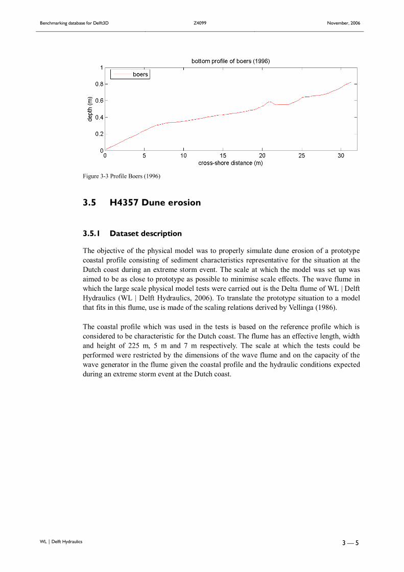
Figure 3-3 Profile Boers (1996)

3.5 H4357 Dune erosion


The objective of the physical model was to properly simulate dune erosion of a prototypecoastal profile consisting of sediment characteristics representative for the situation at theDutch coast during an extreme storm event. The scale at which the model was set up wasaimed to be as close to prototype as possible to minimise scale effects. The wave flume inwhich the large scale physical model tests were carried out is the Delta flume of WL | DelftHydraulics (WL | Delft Hydraulics, 2006). To translate the prototype situation to a modelthat fits in this flume, use is made of the scaling relations derived by Vellinga (1986).

The coastal profile which was used in the tests is based on the reference profile which isconsidered to be characteristic for the Dutch coast. The flume has an effective length, widthand height of 225 m, 5 m and 7 m respectively. The scale at which the tests could beperformed were restricted by the dimensions of the wave flume and on the capacity of thewave generator in the flume given the coastal profile and the hydraulic conditions expectedduring an extreme storm event at the Dutch coast.



Figure 3-4 Initial profile for H4357 tests

Three dune erosion tests were carried out with a water depth of 4.5 m in the flume near thewave board. A water depth of 4.5 m corresponds with a water depth of 27 m in prototype.With a storm surge level of NAP +5 m, this results in a bed level of NAP 22 m near thewave board. The total duration of each test was 6 hours. In all three tests use was made ofthe same initial profile. Sediments with a diameter of D50 = 200.10-6 m, wave heights of Hm0

= 9 m and wave periods varying from Tp = 12 s to Tp = 18 s were applied and test conditionswere determined for the scale of the flume, see Table 3.6. Profile, wave and flow velocitymeasurements were carried out.

Table 3.6 Test conditions H-4357


H4357-Test-01 1.5 4.9 4.5

H4357-Test-02 1.5 6.12 4.5

H4357-Test-03 1.5 7.35 4.5



4 Benchmarking data sets: 2. Fieldmeasurements

4.1.1 Overview

An overview of the implemented field data sets is provided in Table 4.1.

Table 4.1 Overview of laboratory data sets and parametersCode Waves and

set-upCurrent(2DV)

Current(3D)

Concen-trations andtransport

Bottomchange

Sand ridge Sand-ridge

z(x,t)

Duck94 Hrms (t) Uxmean,Uymean

z(x,t)

Grays Harbor z(x,t)Coast3D Egmond

HydHrms u,v

urmsguss, guls

c(z) z(x,t)

EgmondMorph

z(x,t)

Egmond EgmondLong

z(x,t)

Hrms = root-mean-square wave heightu, v = cross-shore and longshore velocity(z) = vertical (i.e., vertical profiles are available)z(x,t) = cross-shore bottom profiles (various moments in time)urms = root-mean-square cross-shore velocityguss = short-wave velocity momentguls = short-wave long-wave interaction velocity momentc = sediment concentration

4.2 Sand-ridge (Tonnon, 2005)

4.2.1 Data set description

From 1982 to 1986 dumpings at Hoek van Holland created an artificial sand ridge, known assand ridge Hoek van Holland, of about 3600 m normal to the peak tidal current and theshore, (location Hoek van Holland in an area with depths between 15 m and 23 m on thenorthern side of the approach channel. In all, 3.5 million m3 sand was dumped over theperiod 1981 to 1986 (Van Woudenberg, 1996). The ridge dimensions just after creation ofthe ridge were: length of about 3600 m; toe width between 250 m and 370 m; heightbetween 1.3 and 4 m; slopes between 1:50 and 1:100 on the southern flank and between1:20 and 1:50 on the northern flank; d50 between 0.15 mm and 0.45 mm. The landward endof the ridge is about 6300 m from the shoreline.



The sand ridge Hoek van Holland is located close to Loswal Noord, which is a dumping sitefor class I and II silt from the Rotterdam harbour mouth. The ridge is perpendicular to thecoast and thus normal to the tidal flow. Primary goals were to study the stability of asubmerged ridge, normal to the tidal flow and to study the effect of the ridge on shorefacesand transport. Also the possible use of submerged ridges as silt traps for backflow of siltfrom Loswal Noord to the port of Rotterdam was an issue. Furthermore similarities withsand waves were to be investigated.

Figure 4-1 shows a schematic plan view of the sounding area and sections, sections are 400m apart and run over the entire length of the sounding area, which is about 2200 m.

Figure 4-1Schematic plan view of the sounding area and sections (section 1 is about 6 km from the coast)

4.2.2 Cases and model set-up

Case

For the reproduction of morphological development section 4 has been chosen. Nearly everyyear bathymetric surveys were carried out. The dataset contains depth measurements forsection 4, over the period 1986-2000. Figure 4-2 shows the morphological development ofsection 4 in 14 years time. The profile measurements in the dataset are named e.g.Ztyear1996.

400 m

N

section 9section 8

section 7section 6

section 5section 4

section 3

section 1section 2

3450 m

2100 m

25 m



Figure 4-2 Measured bed level developments for section 4

Model set-up

For the database the model of Tonnon (2005) has been transformed to a transect model(oriented East-West). The 2DV model consists of 20 layers with a bottom layer thickness of2% at the bottom.

Boundary conditions

To reduce computational time, a representative, morphological tide was derived using themethod of Latteux (1995). The morphological tide gives an optimal representation of theresidual (e.g. yearly averaged) sediment transports. The harmonic components are describedin the input file: morphtide4.bch. The single representative wave from Walstra et al. (1997)was derived to give the best representation of the overall, yearly wave climate at locationEuro-Maas channel by applying the Latteux method to evaluate residual transports.

Table 4.1 Applied wave schematisation

Wave schematisation Hs (m) Tp (s) Direction ( 0)

Walstra et al. (1997) 2.25 6.6 335

Parameter settings

Main differences with the general parameter settings are the following:



Table 4.2 Different parameter settings for Sand-ridge model

Parameter Setting

D50 300 m

Turbulence model Algebraic

sus, bed, susw and bedw 0,4

4.2.3 Results

Appendix 4.2 shows the best result of Tonnon (2005). Most important finding of this modelis that the bed roughness has a dominant effect on the ratio of bed load and suspended loadtransport, on the net annual transport rate and on the migration rate of the ridge; the bedevolution after 15 years can be very well represented by using a variable bed roughness(based on a predictor) neglecting the effect of megaripples resulting in C-values of about 80m0.5/s.

4.3 Grays Harbor (Walstra et al., 2005)


During the Grays Harbor Sediment Transport Experiment (Landerman et al., 2005)instrumented tripods collected time series of waves, near-bottom velocities, and proxies forsuspended sediment concentrations at 6 locations on the inner shelf and upper shoreface(Figure 4-3). Between 4 May and 11 July 2001, the tripods measured conditions during therelatively mild rebuilding phase of the beaches. Data from two stations, (MIA/MIB) inrelatively shallow water (~8 m MLLW) and placed approximately 50 m apart, are used inthis data set for the boundary conditions. During the field deployment, the mean significantwave height was 1.7 m with waves approaching generally from the WNW, conditionssuggesting southerly longshore sediment transport.



Figure 4-3 Chart of study area near Grays Harbor Transect lines for nearshore bathymetric surveys are shown ingreen (after Ruggiero et al., 2003).

Regular topographic and bathymetric surveys quantified both the beach and sandbar changeduring the transition from winter to summer conditions (Ruggiero et al., 2005). Weeklytopographic surface maps (10 surveys) and monthly nearshore bathymetric surveys (5surveys, profiles spaced at 200 m) mapped the active nearshore planform from the toe of theprimary dune (~ 5 m MLLW) to below the limit of measurable annual change (~12 mMLLW) within 4 km of the Grays Harbor North Jetty.


Cases

Two individual cross-shore transects located only 2 km apart illustrate this alongshorevariability in the response of the outer bar (Tran 11 and Tran 20). At Transect 11 the outerbar migrated onshore approximately 175 m between 29 March and 6 August 2001. AtTransect 20 the outer bar migrated onshore only approximately 40 m during this same timeperiod (Figure 4-4).



PROFILE 20

Figure 4-4 Observed cross-shore profile changes during the Spring 2001 experiment (Top: Transect 20, Bottom:Transect 11).

Model set-up

The profile evolution model is run in 2DV mode with a horizontal grid resolution increasingfrom 50 m at the offshore boundary to about 5 m in the surf zone. The vertical grid consistsof ten -layers with an increased resolution near the bed and water surface. The profileevolution model performance was evaluated in Walstra et al. (2005) at both Transects 11 and20 (identical forcing, but different initial profiles) by varying tuning parameters on thepredicted transports and wave induced streaming, increasing the amount of (breaker) delaybuilt into the roller model, and varying the sediment characteristics. In total 40 combinationswere investigated at both cross-sections, leading to the following model parameters:



Table 4.3 Model parameters for Grays Harbor basis model

Parameter Description Setting

fs,c factor on suspended transport due to currents 0.3

fb,c factor on bed load transport due to currents 1.0

fs,w factor on suspended transport due to wave motion 1.0

fb,c factor on bed load transport due to wave motion 0.8

flam breaker delay expressed in local wave length 2.0

fstreaming Scaling factor on wave induced streaming 0.5

D50 Median sediment diameter 220

4.4 Duck (1994)


The data were collected during September and October 1994 near Duck, North Carolina ona barrier island exposed to the Atlantic Ocean. Wave statistics (Hrms, peak period, andenergy) were estimated from a two-dimensional array of 15 bottom-mounted pressuresensors at 8 meter depth. Pressure and velocity observations were obtained at 13 cross-shorepositions extending from near the shoreline to 4.5-m depth. Spatially extensive bathymetricsurveys obtained occasionally with an amphibious vehicle and cross-shore depth profilesobtained continuously with altimeters (Gallagher et al., 1998) show that the bar migratedoffshore 120 m during the experiment, but only 50 m during the first 1000 hrs. Alongshorenon-uniformities in the bar were small for t < 1000 hr, when a broad cross-shore channeldeveloped near the measurement transect. Hereafter large offshore development was seen asa result of storm conditions (Figure 4-5).

Figure 4-5 Bottom profile measurements for DUCK94



The dataset of DUCK94 includes the following parameters: HrmsX, zTtttt (in hours),UxmeanX and UymeanX.

4.4.2 Model set-up

The boundary conditions were conducted from hourly measured water level and waveproperties resulting in time series. The same parameter settings are applied for the model asfor the other datasets in the database. A vertical grid with 11 layers and horizontal grid with4 meter grid width on the seaward boundary to 2 meters on the dry beach was used for thecomputational model.

4.5 Egmond Hydrodynamic


The Egmond site is located in the central part of the Dutch North Sea coast and is dominatedby two well-developed shore-parallel bars intersected by rip channels. In the framework ofthe Coast3D project, two field campaigns were executed, a pilot campaign in spring 1998and a main campaign in autumn 1998 (Van Rijn et al., 2002). During the experiments, alarge variety of instruments, such as pressure sensors, wave buoys and current meters, weredeployed. An overview can be found in Appendix B and in Ruessink (1999). Contrary to thepilot campaign, the main experiment witnessed severe conditions. Large waves, strong windand water level rises due to storm surges were present, resulting in considerablemorphological change (e.g. bar movement, lowering of bar crests and the presence of ripchannels).

Two Coast3D data sets were added to the database: Egmond Hydrodynamic and EgmondMorphodynamic. For both data sets, four cases were defined: pre-storm, storm, post storm,and total period. Egmond Morphodynamic is described in Section 4.6.


Cases

For the reproduction of the hydrodynamics at Egmond during the Egmond Mainmeasurement campaign we have chosen the following cases:

Burst nr. Date-time Tot. days

Pre-storm 9180-9324 18-10-98 12:00 - 24-10-98 12:00 6

Storm 9324-9492 24-10-98 12:00 - 31-10-98 12:00 7

Post-storm 9492-9780 31-10-98 12:00 - 12-11-98 12:00 12

Total period 9180-9780 18-10-98 12:00 - 12-11-98 12:00 25



The burst numbers are based on conventions regarding measurement administration in theCOAST3D project. Burst numbers can be linked with actual dates and times. Burst number9180 corresponds with noon 18 October 1998 and each burst is valid one hour exactly (e.g.burst number 9181 corresponds with 13:00, 18 October 1998). To facilitate comparison ofmodel results and measurements we have chosen burst number 0 as the starting time of themodelling exercise. Consequently, burst numbers divided by 24, yield the correspondinginput for our Delft3D model. For the geographical orientation we have chosen to take theoffshore DIWAR buoy as the origin for the modelling exercise with the positive x-axis to bein the shoreward direction (see Figure 4.1). Positive y is directed alongshore in northwarddirection.

The cases of the hydrodynamic dataset include the following parameters: Hrms, Uxmean,Uymean, Guss and Guls. For Hrms, Uxmean, Uymean, Guss and Guls we includemeasurements from stations 7a, 2, 1a, 1b, 1c and 1d. The measurement stations are locatedat the following positions (Figure 4-6):

Bathymetry (18-10-1998) and instrument locations

-20

-15

-10

-5

0

5

4000 4200 4400 4600 4800 5000

Distance from DIWAR

NA

P

7a21a1b1c1d

Figure 4-6 cross-shore profile and instrument locations

For these parameters we include measured profiles and time series. The time series are givenat the measurement locations measured from DIWAR and are named HrmsXxxxx.tek,UxmeanXxxxx.tek, UymeanXxxxx.tek, GussXxxxx.tek and GulsXxxxx.tek, respectively.The profiles include the data from the measurement locations at a large number of timepoints evenly distributed over the case periods. The profiles are named HrmsTtttt.tek,UxmeanTtttt.tek, UymeanTtttt.tek, GussTtttt.tek and GulsTtttt.tek.

Model set-up

For the database a profile model was constructed (see Roelvink and Walstra, 2004). The2DV model consists of 20 layers with a bottom layer thickness of 2% at the bottom. Themodel is forced with the measured wind and waves conditions. The tide is derived from thetidal station enclosing the Egmond site (IJmuiden and Petten). The model is driven byastronomical components derived using the method described in Roelvink and Walstra(2004).


WL | Delft Hydraulics 4 — 1 0

4.6 Egmond Morphodynamic

4.6.1 Cases

For the reproduction of the morphodynamics at Egmond during the Egmond Mainmeasurement campaign we have chosen the same cases as for the hydrodynamics.

4.6.2 Measurements

The bottom profiles for each case have been included.

4.6.3 Reference model

Reference model is identical to the hydrodynamic version. Futher tuning is expected to takeplace in the course of the present project. This section will be updated accordingly.

4.7 EgmondLong


This dataset consists of yearly profile measurements near Egmond, profile 39.500, over aperiod of 18 years from 1979 to 1997, and associated boundary conditions. A fulldescription can be found in Boers and Walstra (1999).

4.7.2 Model setup

This model has not yet been verified, will be added later (but not in the course of the presentproject).



5 Statistical analysis

5.1 Statistical tool

The question of how well a model performs should be defined in a more quantitativemanner than by judging model performance only visually. This is often sufficient duringearly stages of a project (e.g., parts of the calibration phase), but the final modelqualificattion requires objective quantitative Model Performance Statistics (MPS). Thischapter defines the statistical parameters which are applied in the benchmarking tooldescribed in Appendix A. After selection of a number of models within one test case, thetool creates plot and a statistical file in which model performance for the various models issummarised. In this way a large number of model settings can be evaluated in one table orgraph without having to go into detail of the underlying data. This will give insight into thequality of the predictions, but also provides information on the range of the predictions andthe implications this may have for further use of the model. Later on in this chapter anexample will show the functionality of the model statistical performance.

5.2 Model performance statistics

At present the following statistics have been implemented:

Table 5.1 Model performance statistics

Parameter Description Ranges

Bias Systematic error of the mean low value is low systematic error

SDEV Standard deviation of the error unbiased estimator of the variance

RMSE Root Mean Square Error 0: perfect prediction

MAE Mean Absolute Error 0: perfect prediction

r Correlation 0: no correlation; 1: perfect correlation

BSS Brier Skill Score see below

The mean error ., .,1

1 N

comp i meas ii

ME f fN

and standard deviation of the error

12 2

., .,1

11

N

comp i meas ii

SDEVE f f MEN

of a time series at a point are a useful

measure of model performance for quantities such as wave height or water level. Thestandard deviation is in general not so useful when applied to a bathymetry. A general formof the average difference between measurements is the Root-Mean-Square Error.



1/ 22

., .,1

1 N

comp i meas ii

RMSE f fN

The Mean Absolute Error (MAE) is written as:

., .,1

1 N

comp i meas ii

MAE f fN

The presence of a few outliers will have a greater influence on RMSE than on MAE asRMSE squares the differences. The MAE is therefore less susceptible to the presence ofoutliers. The importance of the outliers may be emphasised by the use of RMSE if it isimportant not to have any points with very large differences between predicted and observedvalues. In general either one set of statistics or the other will be quoted. The set based onsquared errors will, no doubt, become the most widely used due to familiarity, but the setbased on mean absolute values is not so heavily skewed by a few outliers.

The correlation coefficient r is a measure of how strong a correlation is but not howsignificant the correlation is because the distributions of the series are not taken intoaccount.

The performance of a model relative to a baseline prediction can be judged by calculatingthe Brier Skill Score. This skill score compares the mean square difference between theprediction and observation with the mean square difference between baseline prediction andobservation.

2

, ,1

2,0 ,

1

1

1 11

N

b c b miN

b b mi

z zMSE NBSSMSE z z

N

where zb,c is the computed bottom, zb,m is the measured bottom and zb,0 is the initial bottom(variables taken at each cross-shore coordinate i).

Perfect agreement gives a Brier score of 1, whereas modelling the baseline condition gives ascore of 0. If the model prediction is further away from the final measured condition thanthe baseline prediction, the skill score is negative. The BSS is very suitable for theprediction of bed evolution. The baseline prediction for morphodynamic modelling willusually be that the initial bed remains unaltered. In other words, the initial bathymetry isused as the baseline prediction for the final bathymetry. A limitation of the BSS is that itcannot account for the migration direction of a bar; it just evaluates whether the computedbed level (at time t) is closer to the measured bed level (at time t) than the initial bed level.If the computed bar migration is in the wrong direction, but relatively small; this may resultin a higher BSS compared to the situation with bar migration in the right direction, but muchtoo large. The BSS will even be negative, if the bed profile in the latter situation is furtheraway from the measured profile than the initial profile. The limitation shown here is that



position and amplitude errors are included in the BSS. Distinguishing position errors fromamplitude errors, requires a visual inspection of measured and modelled profiles or thecalculation of further statistics (Murphy and Epstein, 1989; Peet et al., 2002). The BSS canbe extremely sensitive to small changes when the denominator is low, in common with othernon-dimensional skill scores derived from the ratio of two numbers.

Table 5.2 Brier Skill Score quantification (Van Rijn et al., 2002).

Qualification Brier Skill Score

Excellent 1.0 - 0.8

Good 0.8 - 0.6

Reasonable fair 0.6 – 0.3

Poor 0.3 – 0.0

Bad < 0.0

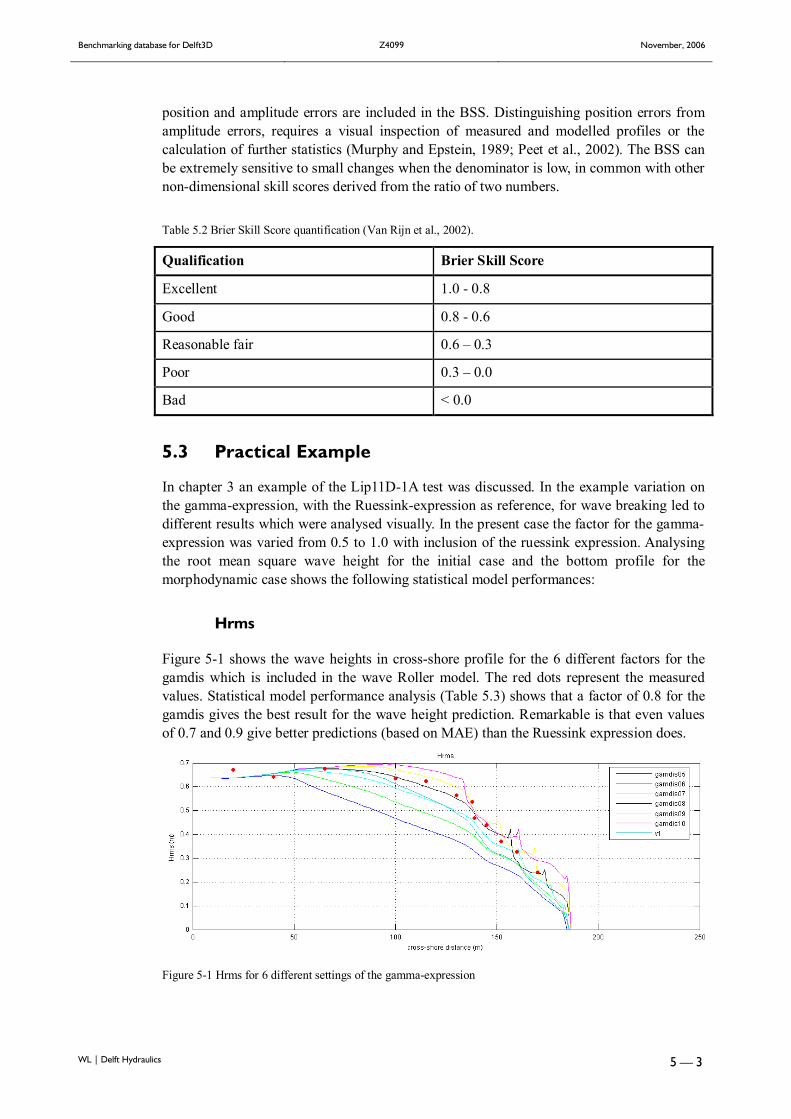
5.3 Practical Example

In chapter 3 an example of the Lip11D-1A test was discussed. In the example variation onthe gamma-expression, with the Ruessink-expression as reference, for wave breaking led todifferent results which were analysed visually. In the present case the factor for the gamma-expression was varied from 0.5 to 1.0 with inclusion of the ruessink expression. Analysingthe root mean square wave height for the initial case and the bottom profile for themorphodynamic case shows the following statistical model performances:

Hrms

Figure 5-1 shows the wave heights in cross-shore profile for the 6 different factors for thegamdis which is included in the wave Roller model. The red dots represent the measuredvalues. Statistical model performance analysis (Table 5.3) shows that a factor of 0.8 for thegamdis gives the best result for the wave height prediction. Remarkable is that even valuesof 0.7 and 0.9 give better predictions (based on MAE) than the Ruessink expression does.

Figure 5-1 Hrms for 6 different settings of the gamma-expression



Table 5.3 Statistical model performance for the Hrms

Test Correlation MAE RMSE

Gamdis = 0,5 0.9106 0.1198 0.1349

Gamdis = 0,6 0.9527 0.0719 0.0832

Gamdis = 0,7 0.9816 0.0339 0.0411

Gamdis = 0,8 0.9904 0.0159 0.0201

Gamdis = 0,9 0.9904 0.0244 0.0287

Gamdis = 1,0 0.9790 0.0348 0.0416

Ruessink et al.(2002)

0.9844 0.0430 0.0525

Bottom profile

In contrast with the performance for the wave height the bottom profile is best predicted forthe Ruessink expression. Although the Brier Skill Score qualifies the model as Reasonableso more calibration of the model is needed, the Ruessink expression gives the best resulthere. For factors of 0.5, 0.8 and 0.9 values are negative, meaning that the predictions are badand that the bed profile is further away from the measured profile than the initial profile.Remarkable is that a gamdis of 0.6 gives better results now than for factors of 0.7 and 0.8.

Figure 5-2 Bottom profile after 12 hours of morphological development



Table 5.4 Statistical model performance for bottom profile development

Test BSS

Gamdis = 0,5 -0.0244

Gamdis = 0,6 0.2330

Gamdis = 0,7 0.0453

Gamdis = 0,8 -0.9576

Gamdis = 0,9 -3.1569

Gamdis = 1,0 -5.1029

Ruessink et al.(2002)

0.3338

It can be concluded that model performance for hydrodynamic and morphodynamic modeldo not automatically have to give similar results. As hydrodynamics differ duringmorphodynamic computing and have large impact on profile development it is ofimportance to predict hydrodynamics right before starting to update the bottom.



6 Recommendations

6.1 Application of the testbank

We think the overhaul of the testbank so that it can now be used for Delft3D is a majorimprovement. Its open structure will allow an easy modification or extension and increasethe efficiency of validation/calibration studies.

Some of the included Delft3D models require further testing and calibration. Especially themorphological models will require constant updating because of changes in the code canhave a relative large (cumulative) impact on the predicted morphology.

6.2 Data sets

The number of datasets has been reduced, only the datasets which benefit the validationhave been included (e.g. similar types of datasets are not duplicated).

There are also opportunities to integrate data obtained with the Argus video technique. Atthe moment we are working on exploring various opportunities to couple the data generatedwith Argus and Delft3D. In the final report we will describe the outcome this activity.



7 References

Arcilla, A.S.-, J.A. Roelvink, B.A. O’Connor, A. Reniers, and J.A. Jimenez, 1994. The Delta Flume’93Experiment. Proc. Coastal Dynamics’94, ASCE, New York, pp. 488-502.

Boers, M., 1996. Simulation of a surfzone with a barred beach; Report 1: wave heights and wave breaking.Communications on Hydraulic and Geotechnical Engineering, Delft University of Technology, theNetherlands.

Boers, M. and D.J. Walstra, 1999. Forecast shoreface nourishment (Draft). RIKZ|WL Report.Bosboom, J., S.G.J.Aarninkhof, A.J.H.M Reniers, J.A. Roelvink and D.J.R.Walstra, 2000. UNIBEST-TC 2.0x,

Overview of Model formulations. WL|Delft Hydraulics report H2305.42.Gallagher, E. L., S. Elgar, and R. T. Guza, Observations of sand bar evolution on a natural beach, J. Geophys.

Res., 103, 3203–3215, 1998.Latteux, B., 1995. Techniques for long-term morphological simulation under tidal action, Marine Geology 126,

129-141Lesser, G., Roelvink, J.A., van Kester, J.A.T.M. and Stelling, G.S., 2004. Development and validation of a

three-dimensional morphological model, Coastal Engineering, 51, 883-915.Reniers, A.J.H.M., J.A. Battjes, A. Falqués and D.A. Huntley, 1997. A laboratory study on the shear instability

of longshore currents. JGR, Vol. 102, No. C4, pp 8597-8609.Rienecker, M.M. and J.D. Fenton, 1981. A fourier approximation method for steady waves. J. Fluid. Mech.,

vol.104, pp. 119-137.Roelvink, J.A. and A.J.H.M. Reniers, 1995. LIP IID, Delta Flume Experiments - a data set for profile model

validation. Delft Hydraulics report no. H2130, Delft.Roelvink, J.A., Th. J.G.P. Meijer, K. Houwman, R. Bakker, and R. Spanhoff, 1995. Field validation and

application of a coastal profile model, Proc. Coastal Dynamics’95, ASCE, 818-828.Roelvink, J.A., M. van Koningsveld, B.G.Ruessink, D.J.R. Walstra and S.G.J.Aarninkhof, 2000. Benchmarking

database, WL | Delft Hydraulics report, Z2897Roelvink, J.A. and Walstra D.J.R., 2004. Keeping it simple by using complex models, 6th Int. Conf. on

Hydroscience and Engineering (ICHE-2004), May 30-June 3, Brisbane, AustraliaRuessink, B.G., 1999. Data report 2.5D experiment Egmond aan Zee. EC Mast Project MAS3-CT97-0086,

Utrecht University, 75 pp.Ruessink, B.G., Walstra, D.J.R., Southgate, H.N., 2003. Calibration and verification of a parametric wave model

on barred beaches. Coast. Eng. 48, 139– 149.Ruggiero, P., Kaminsky, G.M., Gelfenbaum, G., and Voigt, B., 2005. Seasonal to interannual morphodynamic

variability along a high-energy dissipative littoral cell, Journal of Coastal Research, 21(3), 553-578.Tonnon, P.K., 2005. Morphological modelling of an artificial sand ridge near Hoek van Holland, The

Netherlands, WL | Delft Hydraulics report H43079.40Van Rijn, L.C., Walstra, D.J.R. and Van Ormondt, M., 2004. Description of TRANSPOR2004 and

implementation in Delft3D, WL | Delft Hydraulics report Z3748.00.Van Rijn, L. C., D. J. R. Walstra, B. Grasmeijer, J. Sutherland, S. Pan, and J. P. Sierra, 2003. The predictability

of cross-shore bed evolution of sandy beaches at the time scale of storms and seasons using process-based profile models, Coastal Engineering, 47, 295-327.

Vellinga, P. 1986, Beach and dune erosion during storm surges. Ph.D. Thesis, Delft University of Technology;also: WL | Delft Hydraulics report no. 372, December 1986.

Walstra, D.J.R., Renier, A.J.H.M., Roelvink, J.A., Wang, Z.B., Steetzel, H.J., aarninkhof, S.G.J., van Holland,G. and Stive, M.J.F., 1997. Morphological impact of large-scale marine sand extraction (in Dutch).WL | Delft Hydraulics report Z2255, Delft, The Netherlands.

Walstra, D.J.R., Roelvink, J.A. and Groeneweg, J., 2000. Calculation of wave-driven currents in a 3D mean flowmodel. Edge, B. Coastal Engineering vol. 2. ASCE, New York, pp. 1050– 1063.

Walstra, D.J.R., P. Ruggiero, G. Lesser, G. Gelfenbaum, 2005. Modelling nearshore morphological evolution atseasonal scale.



Woudenberg, C.C. van, 1996. De onderwater zanddam bij loswal Noord: gedrag en zandtransport. MScThesis/report NZ-N-92.02, RWS Dir. Noordzee, The Hague, The Netherlands.

WL | Delft Hydraulics, 2006. Dune erosion, large scale model tests and dune erosion prediction method. WL |Delft Hydraulics report H4357, January 2006.


WL | Delft Hydraulics A – 1

A Benchmarking – Tool<matlab.m> is making reference to the matlab file in the work directory.

The benchmarking tool is a Matlab based tool providing a simple way to work with thedatabase. The objective is to facilitate a method for creating new models and analysingmodel results without having to enter all directories. With a simple double-click on thetestbank-executable “testbank.bat”, Matlab will guide the user through a number ofpossibilities. The matlab scripts are all stored in a directory named ‘work’, which is locatedat the level of the test-directories so copying of the full database will include access to thetool.

Double-clicking of the executable will start the procedure and the first screen will provide achoice between the two main user functions: i) making new model run and ii) comparingmodel results. <overall.m>

A.1 Making new models

By choosing the option of making a new model run the user is guided to choose differentcases within a test for which the new model is made. By choosing for example two cases,new models will be made with the same parameters for the two different cases. In this waythe influence of various parameters can be checked on various cases. By entering finish amodel name for the new models have to be entered. Within the chosen cases new directoriesare directly made with the name of the new models and the input files (model settings) ofthe basis model. The interface structure is given in Figure 7-1.

Next step is changing the input files per model. Step by step the user can enter a parameterwithin the input files (*.mdf, *.mor, *.sed and the wavecon) after which the value of thisparameter can be changed. After entering ‘finish’ a new model is created for the differentcases and (dependent on the number of new models) the next model is ready for adapting.Per model a file (report.txt) is created within the model directory in which information isgiven on the changes.

After finishing the preparation of the new models a batch file is created and stored at thelevel of the testbank-executable (run.bat). Double clicking will run the new models andterminate the Matlab tool.



Figure 7-1 Interface structure for setting up new models

A.2 Comparing and analysing model results

By choosing the comparing option first of all the modelpath has to be chosen by selecting atest, a case and a number of models. The structure of the interface is given in Figure 7-2.With the chosen paths, the measured data are read with the <readdata.m> function which isused as input for the further functions. From the names of the TEKAL-files information isstored into a structure array. This information comprises the type of file, the names, valuesbelonging to a location or a time and input for the plotting of the data. If a TEKAL-file isread, named ‘rtfx065.tek’, the function directly reads all files starting with rtfx var(j).type,and stores the names in var(j).names, pulls out the values and stores them in var(j).values.Together with the <makevar.m> function, information matching the var(j).type is added intothe structure:

var(i).type

var(i).names

var(i).values

var(i).fig

var(i).plottype

var(i).mainstr

rtfx

rtfx065.tek, rtfx100.tek, rtfx102.tek…….

65, 100, 102……..

1

f(z)

return flow profiles

The counter (i), refers to the number of data types. With the latter structure as start newTEKAL-files are created in the model directories. In case of cross-shore distribution of



physical data, the data are read from the Delft3D output (trim.dat) and written to a TEKALformat on the numerical grid (grid.grd), e.g. hrms.tek. If the data type is measured on acertain location the closest grid points of the grid are read and data is interpolated to thelocation and written to a TEKAL, e.g. rtfx065.tek. <readD3Doutput.m>

Figure 7-2 Interface structure for model comparison

Plotting model results

The chosen models for comparison are directly plotted with the <showbank.m> function.Within this function the figure names and the figure number have to be entered after whichthe figures are shown on the screen and stored as png-files into the analysis directory on thesame database level.

In Figures 1.1-1.3 examples are shown of plotting results Test 1A of the LIP11Dexperiment. Two different models for the lip11d-hydr\1a model (v1 and gamdis 0,5) areillustrated by the blue and red line whereas the red dots represent the measurements.

Statistical analysis

A statistical tool is built in to compare the model performance of different runs. Thestatistical parameters are the following (Walstra 2004):

Correlation (0: no correlation and 1 perfect correlation)BIAS (0: perfect prediction)Root-Mean-Square Error (0: perfect prediction)Brier Skill Score (0: poor result, 1: excellent results)



The Brier Skill Score (BSS) is only determined when morphological development isanalysed. The parameters are directly stored into a txt-file in the ‘analysis’ directory. (seeTable 7.1). In case of the return flow and the concentration extra files are made with thestatistical parameters.

Table 7.1 Example of statistical result file.

*statistical parameters to evaluate performance, 24-Apr-2006 17:02:07

*for every block, colomns represent the various model results and rows thedifferent statistical methods.

*Line number indicates:

*Line 1: Correlation

*Line 2: RMS error

*Line 3: Brier Skill Score (only in case of morphology)

*Compared models are indicated by:

*Column 1: lip11d-hydr\1a\v1

*column 2: lip11d-hydr\1a\v2

hrms

2 2

0.985748106557224 0.985748106557224

0.0524247202353265 0.0524247202353265

eta

2 2

0.955856590376756 0.955856590376756

0.0193621375896943 0.0193621375896943

stotx

2 2

-0.280713401923819 -0.0575947449037833

9.68688226468971e-006 7.34052150333561e-006


WL | Delft Hydraulics B – 1

B Egmond Coast3D

B.1 Measurements and instrumentation

Data collected concerned:Waves spectrum of wave height, period and direction, near bed

orbital velocities, breaker type, fraction of breaking waves;Water Levels tidal levels, storm surges, wave set-up;Currents depth averaged currents, velocity profile;Water properties salinity and temperature, density structures;Sediment properties grain size distribution, settling velocity and density;Sediment transport transport mode, rates and directions, concentration

profiles;Morphology bed levels before and after events, changes along cross-

shore and longshore transects, cross- and longshoremovement of large bed features such as nearshore breakerbars.

A range of instruments was deployed on site to perform these measurements:

WESPThe WESP (Water En Strand Profiler) is a 15 m high, motorised tripod on wheels with aplatform at the top supporting engine and a cabin with facilities. Survey was conducted fromthe beach out to water depths of 8 m. It is valuable for collection of sand transport data andwill be used for measuring the 3-dimensional bathymetry of the near shore zone. In thisstudy the bathymetry data collected with the WESP is used.The WESP made lanes with a spacing of 50 m in the longshore direction. Depending on thewave conditions measurements were made to a maximum depth of approximately 7 m.Bathymetry data obtained by a ship and measured on the beach was added to the WESP datain order to obtain a complete bottom profile.

CRISCRIS is a trailer towed by the WESP, carrying various instruments for measuring sedimenttransport, water levels, wave parameters and flow velocities. It also takes measurements ofthe sand concentration profiles. The CRIS is 3.5 meters squared and 2.5 meters high. Theinstruments are attached to a movable arm, which can be adjusted in vertical direction toposition the sensors at the desired elevation above the bed.

DIWARThe DIWAR (Directional Wave Rider) buoy is located outside the Egmond area in (almost)deep water. It collects the wave data (height, period, direction). Data used were root-mean-square wave height (Hrms), peak period (Tp) and direction ( ). Gaps in DIWAR data werefilled with measurements from other DIWAR buoys, located at the ‘IJmuiden munitie-stortplaats’ and the ‘Europlatform’.


WL | Delft Hydraulics B – 2

Measuring poles (7a-7f)In total six poles were operating during the measurement campaigns. A number of localvariables and boundary conditions are measured. For example, water level andmeteorological data is collected, the wind velocity and direction measured at this pole wereused in this report. The poles also form a physical barrier for ships and mark and protect themeasurement site.

Maxi frames (2 and 1a-d)The maxi frames measure several parameters. The data used in this study are wave heights,water levels and current velocities. The maxi frames are positioned in the so-called maintransect in the area of interest. A fictive cross-section (normal to the shore-line) at thelocation of the maxi frames was defined as the main transect.

S4-instruments (18a-d, 13a-b, 14a-b, 15)S4-instruments are current and pressure meters. Station 18a and station 18b are located indeeper water (seaward flank of outer bar), station 18c and station 18d are located in the surfzone. Data from station 18a and station 18b was used to estimate the deep water (at DIWARlocation) tidal longshore currents. Station 14a and station 13a are located at the crest of theinner bar, station 14b and station 13b are located at the landward flank of the inner bar, nearthe inner channel.

Only a small selection of the data produced in the main campaign is used in this report. Forour model performance check we only use bathymetry data and hydrodynamic data frommeasuring pole 7a and maxiframes 2 and 1a-d.

Date post:	13-Jan-2022
Category:	Documents
Upload:	others
View:	0 times
Download:	0 times

Rijksinstituut voor Kust en Zee - RIKZ

Documents