Risk Management and Firm Value: Evidence from Weather Derivatives * Francisco Pérez-González Stanford University and NBER Hayong Yun University of Notre Dame January 2011 This paper examines the impact of financial innovation on firm value, investment, and financing decisions. More specifically, we examine the effect of the introduction of weather derivatives on electric and gas utilities, arguably some of the most weather- exposed businesses in the economy. Weather derivatives were introduced in 1997 to help firms manage their weather-related risk exposure. We derive instruments for weather derivative use based on historical (pre-1997) weather exposure. Intuitively, firms whose cash flows have historically fluctuated with changing weather conditions are, relative to other firms, more likely to use weather derivatives once they become available, irrespective of their investment opportunities. Using data from U.S. energy firms, we find that weather derivatives lead to higher market valuations, investments, and leverage. Overall, our results demonstrate that financial innovation can significantly affect firm outcomes and that risk management meaningfully affects valuation, investments, and financing decisions. JEL classification: G30, G32 Keywords: risk management, hedging, derivatives, firm value, capital structure, debt policy, weather risk * Pérez-González ([email protected]) and Yun ([email protected]). We thank Ken Ayotte, Robert Battalio, Jess Cornaggia, Peter Easton, Randall Heron, Dirk Jenter, Tim Loughran, Mitch Petersen, Paul Pfleiderer, Josh Rauh, Paul Schultz, Jeremy Stein, Phil Strahan, Annette Vissing-Jorgensen and seminar participants at the American Finance Association annual meetings, Boston College, Edinburgh University, the Federal Reserve Bank (Board of Governors), Federal Reserve Bank of Chicago-DePaul University, Indiana, Ohio State, Northwestern, Seoul National, Stanford, the University of Aberdeen, British Columbia, Notre Dame, and Toronto. We also thank Laarni Bulan, Howard Diamond, and Paul Schultz for their help with accessing various data sources. All errors are our own.
Transcript
Risk Management and Firm Value:
Evidence from Weather Derivatives *
Francisco Pérez-González Stanford University and NBER
Hayong Yun University of Notre Dame
January 2011
This paper examines the impact of financial innovation on firm value, investment,
and financing decisions. More specifically, we examine the effect of the introduction of weather derivatives on electric and gas utilities, arguably some of the most weather-exposed businesses in the economy. Weather derivatives were introduced in 1997 to help firms manage their weather-related risk exposure. We derive instruments for weather derivative use based on historical (pre-1997) weather exposure. Intuitively, firms whose cash flows have historically fluctuated with changing weather conditions are, relative to other firms, more likely to use weather derivatives once they become available, irrespective of their investment opportunities. Using data from U.S. energy firms, we find that weather derivatives lead to higher market valuations, investments, and leverage. Overall, our results demonstrate that financial innovation can significantly affect firm outcomes and that risk management meaningfully affects valuation, investments, and financing decisions.
* Pérez-González ([email protected]) and Yun ([email protected]). We thank Ken Ayotte, Robert Battalio, Jess Cornaggia, Peter Easton, Randall Heron, Dirk Jenter, Tim Loughran, Mitch Petersen, Paul Pfleiderer, Josh Rauh, Paul Schultz, Jeremy Stein, Phil Strahan, Annette Vissing-Jorgensen and seminar participants at the American Finance Association annual meetings, Boston College, Edinburgh University, the Federal Reserve Bank (Board of Governors), Federal Reserve Bank of Chicago-DePaul University, Indiana, Ohio State, Northwestern, Seoul National, Stanford, the University of Aberdeen, British Columbia, Notre Dame, and Toronto. We also thank Laarni Bulan, Howard Diamond, and Paul Schultz for their help with accessing various data sources. All errors are our own.
1
“Mother Nature is business’s biggest saboteur”1
“Whatever the weather, it's no excuse to lose money” 2
A distinctive feature of modern societies is their ability to understand and control risks
(Bernstein, 1996). Progress, however, does not necessarily eliminate risk exposure. As argued by
Arrow (1965), “nothing is more obvious than the universality of risks in the economic system.”
Economic development has, nonetheless, eased the process of shifting or trading risks. From the
forward contracts in the Bible to exotic financial derivatives, financial innovation has facilitated
risk management.3
The relevance of risk management to firm value is, nevertheless, suspect. While investors
are exposed to uncertain payoffs, portfolio formation allows them to diversify all but market-wide
risks (Markowitz, 1952). As Modigliani and Miller (1958) (henceforth MM) have long stressed,
investors assign higher valuations to firms with positive net present value (NPV) projects but do
not assign a premium for hedged profits that they can themselves, replicate through trading.
Hedging, a pure financial transaction is – at best – a zero NPV project. This logic suggests that
managers should focus on pursuing valuable investments and not on managing risks.
This invariance result, however, stands in sharp contrast to the prominence of risk
management in practice and the rapid growth in financial innovation (Miller, 1986; Tufano,
2003). According to the Wharton-Chase Derivative Survey, nearly 60 percent of large firms
hedge with derivatives (Bodnar, Hayt, and Marston, 1996). Furthermore, derivative markets are
larger than the U.S. stock market capitalization (Office of the Comptroller of the Currency, 2007).
The MM intuition is nonetheless helpful in evaluating hedging decisions. That is, in order
to affect value, firms need to be facing market frictions, such as, transaction costs, informational
asymmetries, or distorting taxes that are alleviated by hedging (Mayers and Smith, 1982; Stulz,
1984; Smith and Stulz, 1985; Froot, Scharfstein, and Stein, 1993; DeMarzo and Duffie, 1995;
Leland, 1998; Graham and Rogers, 2002; among others). Consistent with these ideas, recent
empirical evidence highlights the importance of risk management for firm value. Allayannis and
Weston (2001), Carter, Rogers, and Simkins (2006), MacKay and Moeller (2007), Berrospide,
Purnanandam, and Rajan (2007), and Bartram, Brown, and Conrad (2009), among others, show
that hedging is correlated with higher market valuations.4
1 CFO Magazine, April 1st, 2005. 2 Financial Times, September 17th, 2003. 3 The book of Genesis, Chapter 29 describes a forward transaction between Jacob and Laban, his eventual father-in-law (Chance, 1998). Similarly, Swan (2000) traces the use of derivatives to forward transactions in Ancient Mesopotamia, circa 1750 B. C. 4 Guay and Kothari (2003), in contrast, find evidence that questions the relevance of hedging for firm value, and Jin and Jorion (2006) document insignificant effects of risk management on valuation.
2
The main objective of this paper is to estimate the direct effect of risk management on
firm value, investment, and capital structure decisions. Identifying such effects is empirically
challenging because firms do not randomly select their hedging policies. To overcome those
inference constraints, we examine the impact of risk management on firms’ behavior using a
financial innovation approach. More specifically, we test whether firm value, investment, and
capital structure decisions change with the introduction of weather derivatives.
Weather derivatives are financial instruments whose payoffs are contingent on weather
conditions. Changing weather conditions are a textbook example of a risk-exposure that is both
significant and largely outside management’s control (Stulz, 2003). Yet, until recently formal
markets for weather exposure did not exist.5 Weather derivatives were introduced in 1997 to help
firms manage such weather-related exposures.
To test whether completing the weather exposure market affected decision making, we
focus on electric and gas utilities, some of the most weather-sensitive businesses in the economy.
Heating and cooling demand variation is tightly linked to changes in weather conditions.
Moreover, medium and long term weather predictions are difficult to make.6 Not surprisingly,
energy firms widely recognize the weather as an important risk factor.7 Similarly, survey data
indicates that nearly 70 percent of the end users of weather derivatives are energy firms.8
To identify the effect of weather derivatives, we rank utilities as a function of their pre-
1997 weather exposure. Intuitively, while all firms potentially benefit from hedging, we expect
that those firms whose cash flows have historically fluctuated with changing weather conditions
will be prone to using weather derivatives after 1997, irrespective of their investment
opportunities. Econometrically, we use pre-1997 weather exposure rankings as instrumental
variables (IVs) for the use of weather derivatives in the post-1997 period. Furthermore, such
variation is likely to isolate the insurance, as opposed to the speculative, demand for derivatives.9
To pursue our empirical tests, we use financial data from COMPUSTAT, weather
information from the National Oceanic and Atmospheric Administration (NOAA), and hand-
collected information on the use of financial derivatives since 1997. Our sample includes
information on 203 U.S. utilities.
5 See Roll (1984), for a description of a market that pre-dates weather derivatives, and that closely tracks weather surprises in a single U.S. location. 6 Einstein’s (1941) famous quote, “one need only think of the weather, in which case prediction even for a few days ahead is impossible,” which refers to the complexity of meteorological events, illustrates the point. 7 Over 95 percent of our sample firms state that changing weather conditions are an important factor influencing their annual or quarterly results. 8 Weather Risk Management Association (2005). 9 For evidence on speculation with derivatives, see for example, Géczy, Minton, and Schrand (2007).
3
The key weather variables of interest in the energy sector are cooling, heating, and energy
degree days (CDD, HDD, and EDD, respectively). CDD and HDD values track temperature
deviations above and below 65°F, respectively.10 CDD (HDD) values seek to capture cooling
(heating) demand. EDD is the sum of CDD plus HDD, and proxies for total energy demand.
We begin our analysis by verifying that for our sample firms, moderate weather
realizations significantly affect operating results. We find that mild relative to normal weather
levels are correlated with significantly lower revenues and profits. Interestingly, when we divide
our sample firms into equal-sized quartiles based on proxies for weather exposure, we uncover
substantial heterogeneity in response to mild weather shocks. In particular, while most firms are
unaffected by mild weather realizations, firms in the top weather-exposure quartiles exhibit
dramatic declines in revenue.
The proxies for pre-1997 weather exposure that we use are based on (i) revenue volatility
or (ii) weather-induced volatility. Weather-induced volatility is defined as the product of the
sensitivity of revenue to changes in weather variables (CDD, HDD, and EDD) and its standard
deviation. Using those weather exposure measures, we test for (a) the effect of weather risk on
value, investment, and financing decisions in the absence of weather derivatives, and (b) the
impact of weather derivatives on these outcome variables. We find four main results.
First, in the absence of weather derivatives, weather-exposed firms exhibit significantly
lower valuations and pursue more conservative operating and financing policies than other firms.
Our estimates suggest a value gap for firms in the highest weather-exposure quartiles of around
four percent. Also, we find that weather-exposed firms use less operating and financial leverage.
Specifically, they rarely use nuclear facilities to generate electricity; they rely less on debt
financing and pay fewer dividends than other firms.
Second, we show that pre-1997 weather exposure is a strong predictor of weather
derivative use after 1997. Firms in the top weather exposure quartile are two to three times more
likely to use weather derivatives after 1997 than the least weather-exposed firms. In other words,
we provide evidence that those firms that we would expect to use derivatives for hedging reasons
are indeed more likely to rely on weather derivatives.
10 More specifically, a cooling degree day is given for each degree that the daily mean temperature exceeds 65°F; CDD is zero if the daily mean temperature is below 65°F. The reference value of 65°F is used because historically, when the outside temperature is equal to this value, cooling (electricity) demand is low. Demand increases as daily temperatures exceed 65°F. Similarly, a heating degree day is given for each degree that the daily mean temperature falls below 65°F; HDD is zero if the daily mean temperature is above 65°F. Demand for heating (natural gas) declines above 65°F and increases as daily temperatures fall below this value. Energy degree days are the sum of cooling degree days and heating degree days, and measure all deviation from 65°F to capture extreme hot and cold weather conditions.
4
Third, we show that the introduction of weather derivatives led to a substantial increase
in firm value. The impact of hedging on market-to-book ratios is economically large and
statistically robust. While the IV estimates are at least 20 percent of M-B ratios, we cannot reject
that the causal effect of risk-management on market-to-book ratios is in the 5 to 10 percent level,
as previously reported in the literature. We also assess if the reported results can be alternatively
explained by global warming trends, deregulation, or the use of other risk management tools,
such as interest rate or natural gas derivatives. Yet, after controlling for those effects, we find
robust evidence that weather hedging led to higher market valuations.
Fourth, we find that hedging allows firms to increase investment and to use more
aggressive financing policies. Such results are consistent with the idea that smooth cash flows
allow firms to invest more, either by relaxing borrowing constraints or by allowing firms to
pursue valuable investment projects in low cash flow states. Similarly, they provide evidence that
left-tail cash flow realizations can limit debt capacity due to distress costs or other frictions.
Overall, our results demonstrate that risk management has a meaningful impact on
valuation, investments, and financing decisions. Our cross-sectional and time-series estimates,
suggest that the value of frictions faced by the sample firms due to the weather are in 5-10 percent
of firm value. Our results on hedging and debt capacity are in line with Smith and Stulz (1985)
and Leland (1998). Yet, interest tax shields do not seem to account for the entire effect on value.
The investment effects reported are also consistent with Froot, Scharfstein, and Stein (1993).
Finally, our focus on financial innovation to identify the value of risk management is, to
the best of our knowledge, new in corporate finance literature.11 This approach is potentially
promising for a number of reasons. First, it provides an arguably exogenous variation in the cost
of hedging. Second, it tightens the link between specific risk exposures and hedging instruments,
allowing researchers to understand which specific policies are affected by risk management.
Finally, the results provide a rough estimate of the value of financial innovation, which is an
important and controversial topic in the literature.
The rest of the paper is organized as follows. Section I describes the weather exposure of
energy firms and the various operating and financial policies that can help them mitigate such
risks. Section II presents our empirical strategy and predictions. Section III describes the data.
Section IV examines the impact of mild weather realizations on operating results. Section V
examines the importance of weather risk exposure in the absence of weather derivatives. Section
VI presents the main results of the paper. Section VII concludes. 11 Our approach is closest to Conrad (1989), who examines the effect of the introduction of option contracts on the returns of the underlying securities. She, however, does not analyze a market-wide innovation, nor does she examine the consequence of completing a market on capital structure decisions.
5
I. RISK MANAGEMENT AND ENERGY UTILITIES
I. A. Weather Risk Management and Energy Utilities
According to the National Research Council (NRC), 25 percent of the U.S. gross
domestic product is weather- and climate-sensitive (NRC, 2003). In their report, the NRC
identifies the energy industry as one of the most sensitive sectors in the economy.
Within the energy industry, electric and natural gas utilities are subject to substantial
weather exposure. Heating and cooling demands are tightly linked to changes in weather
conditions.12 Furthermore, regulated utilities are often required to serve such changing demand at
fixed prices. As a result, it is not surprising that weather events have been frequently reported to
significantly affect the cash flows of energy firms.13 In lieu of weather exposure, energy utilities
face the dilemma of determining whether to engage in active risk management and if so, deciding
which hedging tools are appropriate to mitigate their weather exposures.
Prior studies have stressed several rationales for risk management. Smith and Stulz
(1985) and Leland (1998) emphasize the tax benefits from hedging. Froot, Scharfstein, and Stein
(1993) show that risk management can alleviate investment distortions when external financing is
costly. Adam, Dasgupta, and Titman (2007) demonstrate the value of hedging as a strategic tool
in competitive settings. Stulz (1984), in contrast, shows that risk-averse managers with substantial
holdings in their own firm may prefer to hedge firm value.
In terms of tools, utilities can rely on a long array of hedging instruments. Several widely
available tools, however, are effective at hedging price or cost risks, but not volumetric risk
exposure (Brockett, Wang, and Yang, 2005). Such concerns, limit the list of admissible risk
management tools as variation in the weather is primarily a quantity risk exposure.
On the operational side, firms can, for example, diversify their weather exposure by
investing in several geographic regions that differ in their weather patterns. While this approach
is potentially attractive for hedging weather risks, it faces an important tradeoff. Economies of
scale are usually achieved by expanding business activities in nearby communities, which by
construction tend to exhibit similar weather conditions.
12 In this paper, we focus on non-catastrophic weather exposure that result from frequent but relatively low impact events, rather than on catastrophic but infrequent events. 13 Abnormally high (low) cooling degree days have, for example, been reported to boost (harm) the cash flows of the Florida Power and Light Group (Midwest Resources Inc). Source: The Palm Beach Post, July 16, 1998 (The Omaha World-Herald, November 3, 1992). On the other end, high (low) heating degree days have been reported to strengthen (weaken) the cash-flows of Dominion Resources Inc. (Atmos Energy Corp). Source: Dow Jones News Service, April 15, 1994 (The Dallas Morning News, May 11, 1989).
6
Utilities on the other hand, may participate simultaneously in the provision of electricity
and natural gas services. Electricity sales tend to be positively correlated with warm temperatures,
while natural gas sales tend to be negatively correlated with them, providing firms with a natural
hedge. Such strategy, however, may be at least partially ineffective in settings where the negative
correlation between electricity and natural gas sales is less than perfect. Other operating strategies
include the use of flexible generation technologies or the ability to store or trade energy using for
example, long-term contracts. There are, however, some barriers to such approaches. For
example, electricity cannot be efficiently stored. Natural gas can be stored, but the weather
related risk-shifting opportunities are bounded by the limited degree of integration of regional
markets due to transportation costs (Energy Information Administration, 2002)
Energy utilities may alternatively use their capital structure or other financial products to
manage their weather exposure. Firms that are significantly exposed to weather risks may limit
their leverage or hold higher levels of cash to limit their earnings volatility and protect their
valuable investments. Lower leverage or higher cash holdings, however, may limit the firm’s
ability to capture the tax or the disciplining benefits of debt, leading to significant value effects.
Similarly, utilities may use energy derivatives to sell production forward, potentially alleviating
the negative consequences of low energy demand. In practice, natural gas futures are widely used
among utilities. These contracts, however, provide imperfect hedges against weather risks.
Electricity derivatives are, in contrast, virtually nonexistent. 14
Energy utilities can alternatively hedge their climate risk using weather derivatives,
which provide contingent payoffs as a function of weather conditions. Given the interest of
energy utilities in tracking energy demand, it is revealing that the bulk of these contracts are
linked to HDD or CDD values.15 That is, they track deviations in temperatures from a reference
value of 65 degrees Fahrenheit (°F) rather than mean temperatures. Such reference is used
because at 65°F, both cooling and heating demand is low, yet cooling and heating demand are
tightly linked to CDD and HDD values, respectively. 16
Weather derivatives specify five characteristics: (1) the weather index, i.e. HDD, etc; (2)
the period of time, i.e. month, season, etc; (3) the weather station, typically located in a major
city; (4) the dollar value of each tick size, i.e., the amount to be paid per unit of CDD or HDD;
and (5) the strike price, which is indexed as the number of degree days in a period of time.
14 See Energy Information Administration (2002) for a review on these risk management tools. 15 Garman, Blanco, and Erickson (2000). 16 max 0, 65∘ and max 0, 65∘ . As an example, if the average
temperature is 75°F, the corresponding CDD value for the day is 10. If a months’ average daily temperature is consistently 75°F, the corresponding monthly CDD value is 300.
7
The first weather derivative transaction occurred in 1997. 17 Since then, weather
derivatives have been traded over-the-counter (OTC) and starting in 1999, the CME has offered
exchange-traded futures and options. The CME offers monthly and seasonal CDD and HDD
contracts for 42 cities around the world. According to the exchange, weather derivatives are one
of the fastest growing derivative sectors (CME, 2005). The OTC market, in contrast, offers
options and swap contracts that are tailored to the needs of individual firms (Considine, 2000).
While weather derivatives are ideally suited to hedge weather risks, they also face
important tradeoffs (Brockett, et. al., 2005). Exchanged-based contracts are attractive because
they entail lower transaction costs and counterparty default risks. Yet, hedging energy firms may
be subject to basis risks, as the traded weather indexes may not perfectly track the firms’ weather
exposure. OTC derivatives, in contrast, minimize basis risk but may lead to higher transaction
costs and credit risk exposures.
I. B. Weather Derivatives: Example
We illustrate the type of contracts that energy firms can write in the presence of weather
risks with the following example from KeySpan Corp’s 2006 annual report:
“In 2006, we entered into heating-degree day put options to mitigate the effect of fluctuations
from normal weather on KEDNE’s financial position and cash flows for the 2006/2007 winter heating season - November 2006 through March 2007. These put options will pay KeySpan up to $37,500 per heating degree day when the actual temperature is below 4,159 heating degree days, or approximately 5 percent warmer than normal, based on the most recent 20-year average for normal weather. The maximum amount KeySpan will receive on these purchased put options is $15 million. The net premium cost for these options is $1.7 million and will be amortized over the heating season. Since weather was warmer than normal during the fourth quarter of 2006, KeySpan recorded a $9.1 million benefit to earnings associated with the weather derivative.”
KeySpan Corp, now National Grid, provides gas and electric services in the New York
area. In this contract, the weather variable is HDD, the accumulation period is November 2006 to
March 2007, the tick size is $37,500, and the settlement level is 4,159 (seasonal cumulative
HDD). The realized HDD value for the year was 3,916, which gave the contract a payoff at
maturity date of $9.1 million.
Following this example, the strategic use of weather derivatives allows energy firms to
eliminate left tail events that are triggered by specific weather realizations. To the extent that
negative cash flow events distort investment or financing decisions, hedging using weather
derivatives can help firms overcome market frictions and potentially enhance firm value.
17 Houston Chronicle, November 7th, 1997.
8
I. C. Quantity Risk and Informational Problems
As stated above, weather derivatives allow firms to manage their quantity risk exposure.
Beyond utilities, quantity risk may, in some settings, be more relevant than managing price risk.
However, volumetric risk is often difficult to insure due to informational frictions. 18 Firms would
tend to prefer to buy insurance strategically, leading to significant adverse selection problems.
Similarly, insured firms may change their behavior ex-post, generating moral hazard concerns.
A clear advantage of weather-based insurance contracts is that information asymmetry
concerns are minor. First, it is difficult to argue that a given energy utility has superior weather
forecasting abilities relative to other market participants. Likewise, the actions of energy firms are
unlikely to affect weather realizations. As a result, weather derivatives provide a near ideal
laboratory to test for the importance of quantity risk on firm outcomes.
In sum, electric and gas utilities with significant weather-related volumetric risk exposure
can mitigate those risks using a long list of real and financial tools. Hedging weather exposure
with weather derivatives is a relatively new practice that results from financial innovation in the
late nineties. Interestingly, these derivatives are ideally designed to address the volumetric risk
facing energy utilities. Furthermore, unlike other insurance products, weather derivatives face
minor information asymmetry concerns. In the following sections, we empirically test whether
the introduction of weather derivatives had a meaningful impact on firm outcomes.
II. EMPIRICAL STRATEGY
In this section, we describe the empirical challenges faced when identifying the causal
effect of derivatives, and explain our empirical strategy to overcome such inference problems.
II. A. Empirical Challenges
A common approach to examining the effect of derivatives on firms’ outcomes is to use
cross-sectional tests that compare valuation, investment, etc as a function of hedging decisions.
For example:
∗ (1)
where ity is firm value. ithedge is an indicator variable equal to one if the firm uses derivatives,
zero otherwise. If hedging is valuable would be expected to be positive and significant.
18 Cost-related contracts (based on interest rate, commodity prices, etc) are less subject to these concerns.
9
In terms of inference, (1) provides an unbiased estimate of the effect of hedging
whenever derivative use is uncorrelated with other determinants of the key outcome variable. Yet,
a large number of studies starting with Nance, Smith, and Smithson (1993) have shown that
hedging decisions are highly correlated with size, investment opportunities and other financial
conditions. 19 In consequence, OLS or propensity score based estimates are subject to inference
concerns: it is difficult to interpret as an estimate of the causal effect of derivatives.
An alternative way to describe the identification challenges described above is that when
hedging is not random, we implicitly require a rationale for why two otherwise identical firms
would differ in their hedging decisions, even when risk management can meaningfully affect their
businesses. Furthermore, we need such an argument to be unrelated to the firms’ investment
opportunities. Those assumptions, however, are difficult to be satisfied in practice.
II. B. Identification Strategy
In this paper, we exploit variation in weather derivative use that results from both time-
series and cross-sectional sources as explained below:
Time Series Variation
Because weather derivatives were introduced in 1997, they provide time-series variation
in the use of derivatives. This variation allows us to use within-firm specifications:
∗ (2)
where i are firm-fixed effects. Given that (2) captures within-firm variation, is no longer
affected by time-invariant firm traits. is, however, subject to time-varying omitted variable and
endogeneity concerns. To the extent that the econometrician cannot ascertain why some firms
change their hedging strategies over time, remains difficult to interpret as causal.
Time Series - Cross Sectional Variation: Pre-1997 Weather Exposure (“Reduced Form”)
An alternative test for the effect of weather derivatives is to focus on those firms who
from an ex-ante perspective might be expected to benefit from financial innovation. Weather
derivatives allow weather-exposed firms to manage their volume risk, leaving others unaffected.
For this purpose, we rely on a number of proxy variables that capture historical weather
exposure. We then use those proxies in the empirical tests. Formally: 19 See for example, Geczy et al. (1997), Haushalter (2000) and Geczy et al. (2006).
10
∗ ∗ ∗ (3)
where captures ex-ante (pre-1997) or historical sensitivity to weather fluctuations.
also proxies for the potential gains from hedging with weather derivatives after
1997. is an indicator variable that is equal to one after 1997. The coefficient of interest is
. If weather derivatives matter, would be significant. Note that to estimate (3), we do not
require information on actual weather derivatives usage. Yet this formulation implicitly assumes
that weather-exposed firms are more likely to use weather derivatives relative to their peers.
In terms of inference, there are two key identifying assumptions in (3). First, weather
exposure predicts the use of weather derivatives. Second, other than through the effect of
hedging, weather-exposed firms have similar investment opportunities. If those assumptions are
met, is no longer subject to endogeneity or omitted variables concerns.
Instrumental Variables
To obtain the causal effect of weather derivatives, we need to scale by the variation in
weather derivative use generated by the ex-ante weather exposure variables. This is a two-stage
least-squares instrumental variable (2SLS-IV) procedure where the ex-ante weather exposure
control is the instrument for weather derivative use. The first-stage specification is:
∗ ∗ ∗ . (4)
We predict the use of weather derivatives using only information about ex-ante weather
exposures. Note that is zero for the pre-1997 period for all firms; thereafter, it takes the
value of one for weather derivative users. Also, even though is a dichotomous variable,
we estimate (4) using an OLS specification, since a probit or a logit first-stage can harm the
consistency of the IV estimates (Angrist and Krueger, 2001). We then use to test for the
effect of weather derivatives on firm value, investment, or capital structure decisions. Formally:
∗ ∗ (5)
Under the above-described assumptions, wderiv provides an unbiased estimate of the
effect of hedging on outcomes.
11
II. C. Implementation: Estimating Weather Exposure before 1997
As previously discussed, utilities may engage in various operational, capital structure, or
other financial strategies to manage their weather exposures. Yet any residual exposure would
translate into revenue volatility. To the extent that changing weather conditions affect revenue,
we would expect the gains from using weather derivatives to be linked to the following measures:
(a) Volatility (quarterly) of revenue to assets before 1997. Changing weather conditions
would tend to be a primary determinant of revenue volatility. As a result, pre-1997 revenue
volatility would be an important predictor of the post-1997 use of weather derivatives. Revenue
volatility is attractive because it is straightforward to compute, and also because it captures the
total hedging potential. It, however, includes revenue variation that results from other non-
weather sources, which may not affect the post-1997 use of weather derivatives.
(b) Weather-induced revenue-assets volatility (quarterly) before 1997. To focus on
weather volatility, we follow two steps. First, for each firm, we estimate the sensitivity of revenue
to variation in weather conditions (cooling, heating, or energy degree days) before 1997 using the
specification below:
∗ ∗ (6)
where is the quarterly revenue to assets ratio. is the relevant weather measure
of energy, cooling, or heating degree days (EDD, CDD, and HDD, respectively) measured at the
firm level. We control for the level of assets to isolate weather-driven effects. To avoid multi-
collinearity concerns, we estimate separate regressions for each of the weather-related variables.
, , and measure, respectively, the sensitivity of revenue to variation in EDD,
CDD, and HDD, respectively. We herein refer to those estimates as “weather betas.” The absolute
value of weather betas is informative about the firms’ hedging opportunities.
Second, to obtain an estimate of the relevant revenue volatility that is attributable to
weather fluctuations, we multiply the estimated weather betas by the relevant historical standard
deviation. For hedging purposes, the meaningful weather exposure is the product of the absolute
value of weather betas (| |, etc) and the degree of variation in each variable ( , etc).
When estimated before 1997, | | ∗ , for example, captures the historical
weather-induced volatility of revenue that results from EDD. A crucial assumption in this paper is
that this pre-1997 weather-induced energy, cooling, and heating degree day volatility predicts the
relevant post-1997 weather exposures. We anticipate that such exposure would induce firms to
use derivatives as they become available, irrespective of their post-1997 investment opportunities.
12
II. D. Predictions
Based on the above-described specifications, we test four predictions:
1. Weather variation affects the operating results of energy firms, particularly those
with higher revenue or weather volatilities. If utility cash flows are subject to weather- risk,
deviations from normal weather conditions are expected to affect revenue and operating margins.
Moreover, to the extent that weather-exposure measures provide useful rankings of weather risk
exposure, we would expect weather shocks to matter the most for firms with volatile revenue.
2. In the absence of weather derivatives, weather exposed firms are less valuable
and more conservative in their investment and capital structure decisions than other firms.
Weather exposure may affect firm value whenever those risks are not fully diversifiable or if their
presence limits the firms’ ability to overcome market imperfections. For example, idiosyncratic
weather-induced variation in cash flows can limit debt capacity (Smith and Stulz, 1985; Leland,
1998) or prevent valuable investments from taking place (Froot et al., 1993).
3. After the introduction of weather derivatives, weather exposed firms are more
likely to use weather derivatives. Firms whose pre-1997 cash-flows were subject to weather
fluctuations are more likely to benefit from hedging. As a result, they are expected to be more
likely to use weather derivatives relative to other firms.
4. The introduction of weather derivatives leads to a decline in weather-driven
differences in value. To the extent that left tail weather-driven cash flow realizations limit debt
capacity or prevent firms from undertaking valuable investment projects, we expect weather-
related value differences to decline as hedging allows firms to manage their weather exposure. In
other words, risk sharing gains are expected to be larger for firms with greater weather exposure.
III. DATA DESCRIPTION
III.A. Financial and Market Information
We use data from COMPUSTAT firms engaged in the distribution and generation of
electricity and natural gas services (Standard Industrial Classification (SIC) codes 4911, 4923
4924, 4931, and 4932). Given our interest in estimating pre-1997 volatility and weather exposure
measures, we focus on U.S. firms with matching quarterly data for at least 10 years before 1997.
We arrive at a final sample of 203 firms and up-to 8,161 firm-year observations.20
20 Selected variables such as market capitalization or deferred taxes are not available for all firm-years.
13
Summary statistics are presented in Table I, Panel A. To facilitate comparisons over time,
we report information in constant 2008 dollars (Consumer Price Index, adjusted, 2008=100).
Average (median) total assets are $5.2 (2.7) billion. Mean (median) revenue is $2 ($1.1) billion.
The mean (median) market capitalization (common shares outstanding times their closing price)
is $2.3 ($1.1) billion. As expected, utilities are larger than the average COMPUSTAT firm.
We follow the pre-existing literature in using market-to-book (M-B) ratios as a measure
of value. The average M-B is 1.08, with a standard deviation of 0.21. 21 Utilities are the textbook
example of firms with tangible assets and stable cash flows. As a result, it is unsurprising that
they use substantial amounts of leverage. The mean and median book leverage relative to assets is
0.41, with a standard deviation of 0.09. Net debt to assets ratios (book leverage minus cash and
short-term investments) are on average 0.38 (median 0.37). The average and median operating
profitability to total assets ratio (OROA) is 0.12. OROA’s standard deviation is 2.6 percent.
Table I, Panel A also includes information on investment and dividend decisions. The
mean (median) ratio of capital expenditures to assets is 0.074 (0.067). However, capital
expenditure information is not available for all firm-year observations. The growth rate of assets
or net investment rate is, in contrast, consistently available, with an average (median) value of
0.072 (0.061). The fraction of energy firms with nuclear plants is 0.37. This indicator variable is
constructed using the COMPUSTAT industry-specific files. This information is only consistently
reported until 1994. Lastly, the average ratio of dividends (common) over assets is 0.03.
III.B. Weather Data
We obtain weather data for all 344 climate divisions in the contiguous U.S. from the
National Oceanic and Atmospheric Administration (NOAA). NOAA has monthly temperatures,
cooling and heating degree day data from 1895 to the present. We also compute energy degree
days as the sum of CDD and HDD values. To match firms with weather sites, we use latitude and
longitude information on the location of the firms’ main business, and of each of the weather
stations. For each firm, we find the closest climate division in terms of their geodesic distance and
use its weather information. 22 NOAA reports the latitude and longitude data of all climate
divisions. COMPUSTAT reports the firms’ zip codes. To determine the approximate latitude and
longitude location of each zip code, we rely on data from the U.S. Census Bureau.23
21 M-B ratios are a proxy for Tobin’s Q (Tobin, 1969), the market value of assets relative to their replacement costs. M-B ratios are calculated as the ratio of the sum of the book value of assets, plus the market value of equity, minus the sum of the book value of equity and deferred taxes over book assets. 22 See Vincenty (1975) for computing geodesic distances between locations. 23 http://www.census.gov/geo/www/gazetteer/places2k.html#counties.
14
The annual weather information is summarized in Table I, Panel A. The annual mean
(median) CDD value is 1,040 (809), with substantial variation around this average (standard
variation of 809 degree days). The mean (median) annual HDD level for the firms in the sample
is 5,170 (5,577) with a standard variation of 1,965. Average (median) annual EDD values are
6,210 (6,386) and the EDD standard deviation is 1,381.
III.C. Information on the Use of Financial Derivatives After 1997
The data on the use of financial derivatives in the post-1997 period is hand-collected
from the Securities and Exchange Commission (SEC) filings using the LexisNexis Academic
application. We use keywords to identify those firms that rely on weather derivatives, as well as
those that use natural gas and interest-rate hedging instruments. 24
While we do not have data on actual derivative exposure by firm, we use indicator
variables to classify firms as derivative “users” whenever SEC filings describe such contracts.
Table I, Panel B reports information for the post-1997 sample or 1,633 firm-year observations.
Weather derivatives were used by one quarter of the sample firms. This usage level suggests that
weather derivatives are unlikely to be beneficial for all sample firms and that, following the logic
described in the previous section, we can potentially focus on differential exposure to estimate the
likely gains from their usage. Natural gas derivatives were used by 57 percent of the sample
firms. The fraction of interest rate derivatives users was 0.87. The fact that the latter ratio is the
largest is not surprising given the magnitude of the interest-rate swaps markets.
III.D. Weather Conditions and Energy Units: Average and Regional Variation
As a first pass on the link between weather conditions and energy sales, Figure 1 plots the
monthly sales of electricity (Panel A) and natural gas (Panel B) in 2005, and their corresponding
mean temperatures in the U.S. To emphasize quantity and not price variation, we report energy
units sold. Figure 1, Panel A shows that electricity sales peak during the summer, reflecting the
seasonal demand for air conditioning. Panel B shows that natural gas sales peak during the winter
months, reflecting the seasonal heating demand. Figure 1, in Panels A and B, shows a strong
correlation between monthly average temperatures and energy sales in units. The correlation is
0.56 and -0.8 for electricity and natural gas, respectively.
24 For each of the weather, natural gas, and interest-rate contracts, we use the following accompanying keywords: derivatives, forwards, futures, hedging, options, and swaps. For example, for interest-rate derivatives, we used “interest-rate derivatives,” “interest-rate forwards,” “interest-rate futures,” “interest-rate hedging” “interest-rate options,” and “interest-rate swaps.”
15
Figure 2 provides a graphical justification for the widespread use of CDD and HDD
values to proxy for electricity and natural gas demand, respectively. Panel A plots monthly
electricity sales relative to the peak August value (August units=100) and the corresponding
monthly CDD levels. Beyond the already stressed seasonality of electricity sales, it shows a tight
correlation between electricity units and CDD values of 0.82. Similarly, the correlation between
natural gas units sold (January units=100) and HDD values is high or 0.88.
In Figure 3, we use data from three states, California, Louisiana, and Montana, to
highlight the sectional differences in terms of weather exposure. Panel A shows that electricity
sales in Louisiana are highly seasonal. Summer electricity volumes are over 40 percent higher
than those in March, which occurs in more than half a dozen states. In contrast, Panel B shows
that monthly natural gas sales are stable. Figure 3 also shows that Montana energy sales display
contrasting patterns: monthly electricity sales are relatively stable while natural gas sales are
remarkably seasonal. January natural gas sales were four times July’s sales. Lastly, California’s
energy sales reveal a moderate level of seasonality both for electricity and natural gas sales.
Overall, Figures 1-3 suggest four issues. First, weather variation and energy demand are
tightly linked. Second, CDD and HDD values track energy demand more closely than average
temperatures. Third, some regions may be more subject to weather-induced variation than others.
Finally, the relevant weather and energy sales variables differ across the U.S.
IV. CHANGING WEATHER CONDITIONS AND CASH FLOW EFFECTS
To test for the effect of changing weather conditions on operating performance, in Table
II, we examine the effect of “low” energy degree days or “weather shocks” on revenue, profits,
investments and payout decisions. The weather shock indicator variable is firm-specific and is set
to one for the lowest quintile of annual EDD observations per firm, zero otherwise (i.e. each firm
has one “shock” per five observations). We focus on the effect of mild EDD values to provide a
simple within firm test that is meaningful independent of a firm’s main weather exposures (CDD
or HDD). Table II, Column I shows that mild weather realizations lead to lower levels of revenue.
The effect is statistically significant but modest in economic terms: mild weather leads to an
average decline of two percent in revenue. Table II, Columns II and III confirm that mild weather
negatively affects cash flows in a significant way. Both operating return on assets and the level of
operating profits decline when the weather is mild. The effect on profits is also modest. Table II,
Columns IV and V, in contrast, cast doubt on the notion that mild weather conditions
meaningfully affect dividend or investment decisions.
16
To assess whether Table II reports mild across the board weather effects on cash-flows or
heterogeneity in terms of weather shocks, we turn to the weather exposure variables described in
Section II, which capture the un-hedged quantity risk exposure faced by energy firms. Table III,
Panel A provides summary statistics for various measures of weather exposure. The risk measures
include (a) revenue volatility (standard deviation of quarterly revenue to assets), (b) CDD, HDD,
and EDD weather betas (absolute value of the estimated coefficient of CDD, HDD, and EDD on
revenue to assets), and (c) CDD, HDD, and EDD weather-induced volatility (weather betas times
the relevant historical standard deviation). All measures are estimated using pre-1997 data.
Table III, Panel A provides consistent evidence that the reported exposure measures tend
to vary substantially. Mean revenue to assets volatility is 0.024, but it is 0.01 (0.11) in the 10th
(90th) percentile. Weather betas also exhibit substantial dispersion. Average CDD or EDD betas,
for example, are 0.9 and 0.3, respectively. Yet the 10th and 90th ranges are 0.06 and 3.2 for CDD
betas and 0.01 to 0.94 for EDD betas. Similarly, weather-induced volatility varies greatly. The
10th and 90th percentiles are 0.17 and 30.6 for CDDs, 1.62 and 160.7 for HDDs, and 2.3 and 162.4
for EDDs, respectively. While these weather exposure numbers may be difficult to interpret in
isolation, the relative ranks that they generate are intuitive: they are orderings of risk exposure.
Interestingly, Table III, Panel B shows that revenue and weather-induced volatility
measures are highly correlated. For example, the correlation between revenue and weather
volatility is 0.79, 0.93, or 0.90 depending on the weather measure CDD, HDD, or EDD,
respectively. Moreover, the CDD-HDD (HDD-EDD) volatility correlation is 0.84 (0.97). Such
correlations corroborate that these volatility measures capture weather-induced variation.
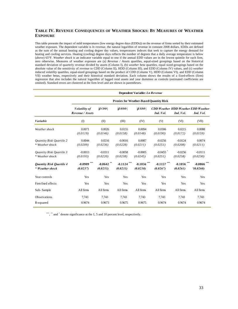
In Table IV, we verify the relevance of the weather exposure measures using the weather
shock approach of Table II. In each column, we analyze the effect of one weather risk measure at
a time, but we refer to them generically as “quantity risk” measures. In each case, we (a) divide
our sample firms into four quartiles based on each risk measure, (b) interact each quartile with the
firm-specific “shock” variable, and (c) test which quartile exhibits the largest decline in revenue.
As in Table II, these are fixed-effects specifications with year and size controls.
Table IV, Column I examines the consequences of mild EDD values for the different
quartiles sorted by revenue volatility. The evidence shows that weather shocks lead to
insignificant effects on all but the most volatile utilities. For firms in the most volatile quartile,
however, weather shocks lead to a drastic decline in revenue of 9.1 percent, significant at the one
percent level. Columns II, III, and IV show that ranking weather exposure based on weather betas
generates similar results. In each case, the most exposed quartile drives the entire decline in
revenue. Further, the effect on this latter group of firms is consistently large and significant.
17
Table IV, Columns V, VI, and VII show the results of moderate EDD values on firms
when we sort them by CDD, HDD, and EDD weather-induced volatility, respectively. As before,
the most weather sensitive group exhibits consistently large and robust declines in revenue. Mild
EDD values lead to a 9 to 12 percent decline in revenue for the most weather-sensitive firms.
These effects are significant at the one percent level. The results show that irrespective of the risk
measure used, high weather exposure quartiles exhibits high cash-flow-weather sensitivities.
In sum, the results from Tables II and IV provide empirical support for prediction 1.
Namely, that changing weather conditions meaningfully affect operating results and that weather
exposure can be measured by using revenue or weather-induced volatilities. Finally, the fact that
only a fraction of firms are subject to cash flow volatility provides information on which firms are
expected to be subject to the largest distortions, if any, in terms of value, or investment and
capital structure decisions. We turn to those tests next.
V. PRE-1997 WEATHER EXPOSURE: VALUE, INVESTMENT, AND CAPITAL STRUCTURE EFFECTS
V. A. Weather Risk in the Absence of Weather Derivatives: Market-to-Book Analysis
In Table V we examine the effect of weather risk exposure on firm value (M-B ratios)
prior to 1997. Given that weather exposure variables are time-invariant, we rely on controls to
account for firm heterogeneity rather than on firm fixed-effects. Table V, Column I shows that
firms in volatility quartiles 3 and 4 trade at a significant discount. Yet, introducing year dummies
reduces the estimated value gap and only firms in quartile 4 robustly underperform. Table IV
Columns III and IV show results controlling for regional and state dummies, respectively. In
those columns, the estimated discounts for the most volatile quartile are in the 3-4 percent range.
Beyond weather variables, the effects of size, profitability, and investment opportunities controls
are as expected: negative for assets, and positive for OROA and investments.25
Using EDD weather volatility as an alternative measure for weather exposure (Columns
V and VI) confirms that weather-sensitive firms trade at a discount of four percent, significant at
the one percent level. Using the log of market value as a dependant variable, Columns VII and
VIII confirm that weather exposed firms had lower valuations. In results not shown, we examine
the linear impact of revenue volatility, EDD, CDD, and HDD volatility, respectively. In every
case, weather exposure significantly effects valuation. Yet, given the shock and M-B results, we
favor the quartile specifications as they stress the firms that drive the relevant effects.
25 The number of observations in Table V declines relative to Table IV because M-B ratios are not available for all firms. Yet, the results in Table IV are unchanged if we solely focus on firms with M-B values.
18
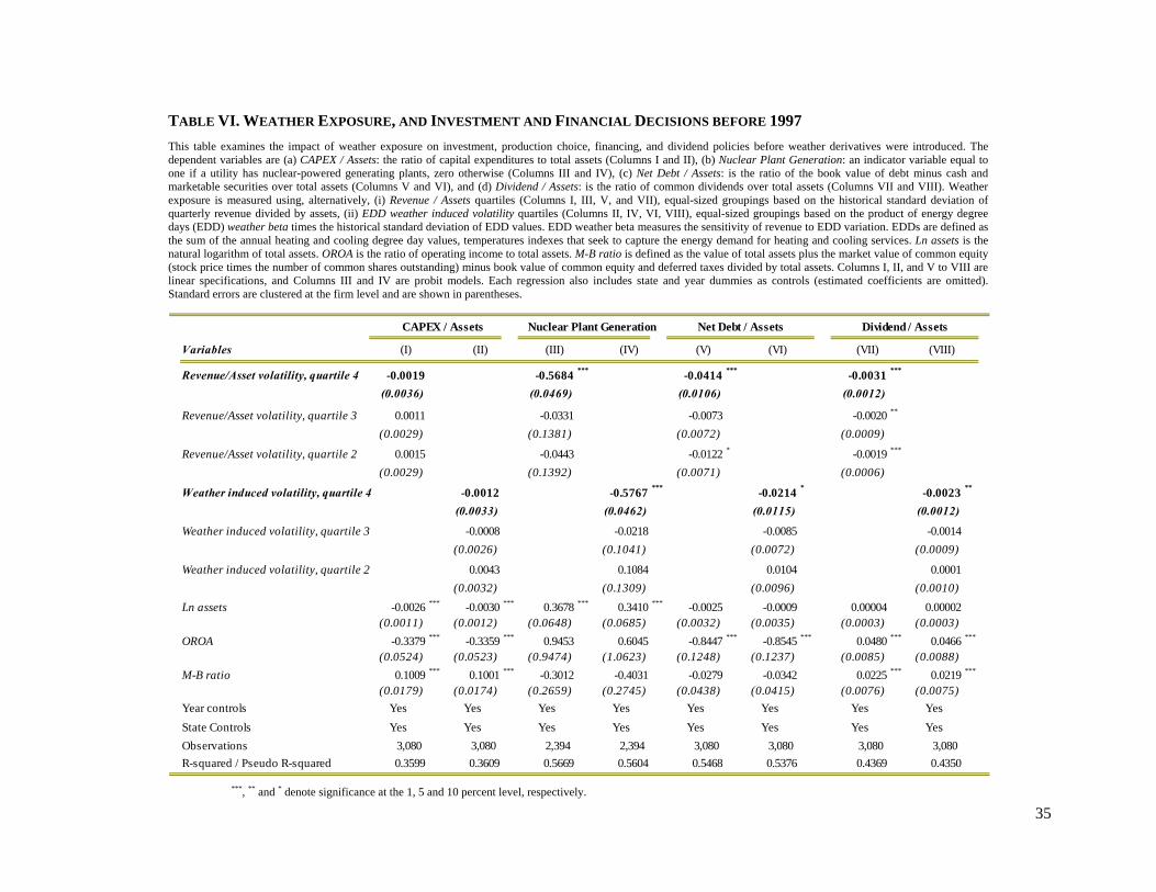
V. B. Weather Risk in the Absence of Weather Derivatives: Investment and Financing Decisions
To assess if the market value differences reported above reflect distortions in operating or
financial decisions, Table VI examines the effect of weather exposure on investment decisions, as
well as on financing and dividends policies. In every specification, we use year-specific and state
dummies to control for aggregate and regional effects, and assets, OROA, and M-B ratios, to
control for size, profitability, and investment opportunities, respectively.
The results in Table VI, Columns I and II cast doubt on the idea that weather exposure
affects firms’ investment decisions. The estimated effect of weather risk on the ratio of capital
expenditures to assets is not different from zero at conventional levels and is small in economic
terms. To further test for the effect of weather risk exposure on investments, we examine the use
of nuclear plants for electricity generation. Nuclear plants are interesting as a technology choice
because they are relatively inflexible. As a result, weather volatility would tend to make them
unattractive. Consistent with this notion, Table VI, Columns III and IV show that quartile 4 firms
are 57 percentage points less likely to use nuclear technologies, relative to their peers. The
evidence indicates that weather exposure distorts investments against inflexible technologies.
The effect of weather exposure on capital structure (net debt) and payout policy
(dividends to assets) is reported in Table VI, Columns V to VI and VII and VIII, respectively.
The evidence shows that firms in the most weather exposed quartile have debt ratios that are 2 to
4 percentage points lower than their peers, consistent with the idea that creditors care about left-
tail events. Economically, such estimates imply a 6 to 11 percent gap in leverage ratios. Similarly,
we find that weather sensitive firms have lower dividend payments relative to their peers. The
differences are in the 0.002 to 0.003 range, significant at conventional levels. These estimates
suggest that firms in the most volatile group pay 8 to 10 percent fewer dividends than other firms.
The results from Table VI show that investment and financial distortions may be central
to understanding the negative effects of weather exposure on value. While utilities with high
weather exposure have investment levels that are comparable to those of their competitors, their
types of investments are distorted towards technologies with less operating leverage. Similarly,
the presence of substantial weather risk induces firms to use less aggressive financial structures,
which may prevent firms from seizing tax or incentive-based benefits. While the estimated
coefficients in Table VI are subject to several inference concerns, we can use them to evaluate the
contribution of the interest tax shields for value differences. Specifically, at historical or existing
tax rates, a higher leverage ratio of 2-4 percentage points in terms of assets is unlikely to explain
the differences in value in the 4-6 range.
19
Overall, the results provide empirical support for prediction 2. Namely, absent weather
derivatives, weather-exposed firms are less valuable and more conservative than their peers. We
now turn to testing whether these distortions were relaxed by financial innovation.
VI. MAIN RESULTS
VI.A. Derivative Use and Firm Value: Within Variation
Before implementing our main empirical tests, we provide a benchmark estimate of the
effect of weather derivatives on value using the within-firm variation specification described in
specification (2) of Section II. We test whether the M-B ratio of those firms that endogenously
decided to use weather derivatives after 1997 increased their valuations. In Table VII, we use a
weather derivative indicator variable that is equal to one if the firm used weather derivatives after
1997, and is zero otherwise. Naturally, this variable is set to zero before 1997. The variable of
interest is the interaction between this indicator variable and the post 1997 variable. As in
previous specifications, we control for time, size, profitability, and investment effects. Table VII,
Column I shows that weather derivative users experienced a significant increase in value of 5.2
percentage points. This estimate is not driven by time-invariant firm traits. Yet, as outlined in
Section II, it is potentially subject to time-varying endogeneity or omitted variables concerns.
To partially assess the severity of such concerns, in Table VII, Columns II to V, we test
whether those firms that use other financial derivatives after 1997 gain in terms of value relative
to their peers. If the use of derivatives is a symptom of superior business prospects, we would
expect any hedging strategy to be correlated with higher valuations. However, in Columns II, III,
and VI, we fail to find significant economic or statistical effects for the use of interest rate
derivatives. In Columns IV to VI, we show that natural gas derivatives led to higher M-B ratios in
the 3-4 percent range, but this effect is not robustly significant. Interestingly, the effect of weather
derivatives is unaffected by those added controls. Lastly, the estimated coefficients on size,
profitability, and investments carry the previously reported and expected signs.
Using the natural logarithm of market valuations as an outcome variable, in Table VII,
Column VII, we confirm that weather derivatives correlate with significantly higher market
valuations and that the results shown in Columns I to VI are not driven by variation in the
denominator of the M-B ratios. Surprisingly, we report that the use of interest rate derivatives is
correlated with significantly lower M-B ratios. Such a result is arguably reflective of omitted
variables concerns, as firms are unlikely to voluntarily use derivatives to lower their firm value.
In contrast, natural gas derivatives are correlated with higher firm values.
20
The results shown in Table VII suggest that financial innovation targeted at the specific
risks facing energy firms was conducive to higher valuations. The estimates on the value of
hedging are consistent with those reported by Allayannis and Weston (2001). Yet, those
specifications highlight the inference concerns of using endogenous hedging variation. To address
those shortcomings, we turn to our main empirical tests.
VI.B. Weather Exposure and Firm Value (“Reduced Form”)
The central idea of this paper is that financial innovation allowed weather-exposed firms
to shield a portion of their weather risk. To the extent that weather exposure rankings do not
change over time, we would expect that those firms that pre-1997 were subject to meaningful
weather exposures would increase in value as weather hedging contracts become available. To
test for this hypothesis we interact the historical weather exposure measures of Table III with a
post-1997 dummy. As in Table IV, we refer to weather exposure variables collectively as
“quantity risk” measures. In each Column I through V, we report a different proxy and each
variable is described at the top of each column.
Table VIII, Columns I and II present results for the two main measures of weather
exposure: revenue and EDD weather-induced volatility, respectively. The results show that
quartile 4 firms, which were reported to underperform before 1997, do indeed gain following the
introduction of weather derivatives. The estimated effect is economically large and statistically
significant: M-B ratios increase by 10 percentage points, significant at the one percent level. As
in the pre-1997 period, firms in weather-exposure quartiles 2 and 3 do not exhibit differential
value differences, which may confirm that moderate exposures are relatively easy to hedge using
other operating and financial tools. The post-1997 indicator variable shows that all energy firms
increased in value. Other controls are robustly significant and exhibit the expected signs.
Table VIII, Columns II to IV show that firms whose cash flows and market valuation
were affected by weather exposure before 1997, gain as weather derivatives are introduced,
irrespective of the proxy for weather exposure used: EDD, CDD, or HDD weather-induced
volatility. The estimated coefficients are in the 0.10 to 0.13 range and always significant at the
one percent level. An alternative but arguably noisier measure of weather exposure is using an
indicator variable equal to one if variation in energy degree days had a bearing on explaining
revenue volatility, irrespective of the sign of this relationship. Table VIII, Column V confirms
that while such a weather beta does not account for the total variation in EDD over time, it still
does corroborate that weather-exposed firms gained in the post-1997 period.
21
Table VIII provides robust evidence that the weather risk discount reported in Table V
disappeared after 1997. Under our baseline assumptions, these reduced-form estimates are not
subject to inference concerns, and as such provide causal evidence that hedging affects value.
VI.C. Weather Derivatives and Firm Value: Instrumental Variables
The idea of the 2SLS-IV approach is to establish a direct link between weather
derivatives and firm value. If weather derivatives are used to hedge weather risks, their usage
would be expected to be more prominent among weather-exposed firms. If that were the case, we
could exploit the differential variation in weather derivative use that results from this ex-ante
exposure to assess the causal effect of weather derivatives on value. We proceed with this test by
first testing whether pre-1997 weather exposure variables predict weather derivative use after
these financial derivates were introduced.
First Stage: Ex-Ante Weather Exposure and Weather Derivative Use
Table IX examines the effect of the previously described measures of weather exposure
on the use of derivatives after 1997. In all specifications, the dependent variable is an indicator
variable that in the post-1997 period takes the value of one for firms using weather derivatives
and is zero for both non-users and all pre-1997 observations.
Table IX shows that the use of weather derivatives increases with weather exposure,
irrespective of how such exposure is measured. Using revenue volatility as proxy for weather
exposure, we report, in Table IX, Column I, that firms in quartiles 3 and 4 are 18 and 22
percentage points, respectively, more likely to use weather derivatives than the least weather
exposed quartile of firms, a difference that is significant at the five percent level.
A tighter test on the effects of weather exposure on weather derivative use is to focus on
weather-induced volatility, which captures the portion of revenue volatility that is attributable to
the weather. In Table IX, Column II, we show that EDD weather-induced volatility quartiles 3
and 4 are 19 and 22 percent, respectively, more likely to use weather derivatives than quartile 1.
This difference is statistically significant at the five and one percent levels, respectively.
Economically, these results show that firms in the most weather-sensitive quartile are over 2.5
times more likely to use weather derivatives than those in quartile one.
Table IX, Columns III and IV confirm that weather exposure does in fact predict weather
derivative use. Specifically, firms in the top two CDD and HDD quartiles exhibit higher rates of
weather derivative use after 1997 than the energy firms in the bottom two groupings. The rate of
weather derivative use among firms in the top weather exposure quartile is the 0.32-0.35 range,
22
while the equivalent rate for firms in the bottom quartile is only 0.13-0.14. Table IX, Column V
shows that even a rough proxy for historical weather exposure, such as having a statistically
significant EDD weather beta, provides large variation in weather derivative use. In particular,
those firms with significant weather betas in the pre-1997 period are 26 percent more likely to use
weather derivatives than other firms, also significant at the one percent level.
Consistent with prediction 3, Table IX provides robust evidence that pre-1997 weather
exposure rankings are important determinants of weather derivative use after 1997. As such, we
are able to confirm that those firms that from an ex-ante perspective would be expected to benefit
from “completing” the weather exposure market are indeed using these financial instruments
more frequently than other firms. Having shown that weather exposure begets usage of weather
derivatives, we now examine the consequences of risk management for firm value.
Second Stage: Weather Derivative Use and Firm Value
Table X presents the main results of this paper. Across specifications, we use market-to-
book ratios as benchmarks for firm value. We exploit variation in weather derivative usage
resulting from (a) the introduction of weather derivatives in 1997 and (b) the pre-1997 weather
exposure measures described earlier. We use fixed-effects specifications, with controls for size,
profitability, and investment opportunities, as well as time effects.
Table X, Columns I and II present the effects of weather derivatives on firm value using
EDD weather-induced volatility quartiles as instruments, our benchmark specification. The
results show a positive and arguably causal effect of financial derivatives on value. The point
estimates are 0.39 and 0.36, depending on whether we include the firms’ concurrent investment
rate as a control, and both are significant at the five percent level. As it is common with IV
estimates, the standard errors are large since they rely on fewer observations to estimate the effect
of derivatives. As a result, we cannot reject the possibility that the true causal effect of weather
derivatives is, for example, in the 5 to 10 percent range as previously reported in the literature.
While we have stressed the potential advantages of using EDD weather-induced quartiles
as a benchmark proxy for quantity risk exposure, we also report the results using revenue-based
volatility quartiles (Columns III and IV) and EDD weather betas (Columns V and VI) as
instruments. Depending on the source of variation used, the estimated effect of derivatives ranges
from 0.22 (revenue volatility) to 0.31 (EDD weather beta) percentage points, significant at the
five percent level. These findings show that there are substantial risk-sharing gains that result
from targeted financial innovation. Also, across specifications, firm size, profitability, and
investment rate controls exhibit the expected signs and significance. Size is negatively related to
23
M-B ratios. Higher profitability and investment rates robustly relate to higher valuation. The
results in Table X provide empirical support for prediction 4, which anticipates that weather
derivatives lead to economically large and statistically significant effects on value.
A potential challenge to reported effects of weather derivatives on firm value is that the
pre-1997 weather exposure rankings may affect post-1997 M-B ratios through other channels. For
example, inference may be challenged by a combination of changing climate conditions due to
global warming, variation in business opportunities due to deregulation, or a reduction in risk
exposure due to other hedging technologies, among others.
In Table XI, we examine the robustness of our results against alternative hypotheses.
Throughout our specifications, we provide 2SLS estimates where the IVs are EDD weather-
induced volatility quartiles. However, all the results are robust to using, for example, historical
revenue volatility quartiles as alternative instruments. In Table XI, Columns I and II, we examine
whether the reported effect may be driven by differential cooling or heating degree day
conditions. To test for this effect, we use the natural logarithm of CDD and HDD values,
respectively. The estimated coefficient of CDD on M-B ratios is positive and significant,
suggesting that higher cooling demand lead to higher market valuations. Yet the effect of weather
derivatives on value is unaffected. The effect of HDD is, in contrast, insignificant. In any event,
we continue to report a robust effect of weather derivatives on value.
We also use information from the Energy Information Administration (EIA) to test
whether state level deregulation of electricity and natural gas markets drives the reported effects
on market valuation.26 Table XI, Column III includes indicator variables that are equal to one for
the observations where the relevant state-year has experienced electricity and natural gas
deregulation, and are zero otherwise. The results show that deregulation by itself did not affect
value and, more importantly, it did not affect the estimated effect of weather derivatives.
To further control for differences in the structure of deregulation, in Column IV, we
include indicator variables associated with specific electricity (Fabrizio, Rose, and Wolfram,
2007) and natural gas deregulation events. These include having access to retail, industrial, or all
electricity consumers or having pilot, partial, or complete choice in natural gas markets. Each
dummy is set to one for the observations where, according to the EIA, the relevant state-year has
experienced deregulation. While we find that complete access to all consumers in electricity led
to a significant increase in M-B ratios of 7 percentage points (other effects are insignificant), we
do not find that such deregulation indicator variables affect the estimated coefficients of interest. 26 Information on electricity and natural gas deregulation was obtained from the following EIA websites: http://www.eia.doe.gov/cneaf/electricity/page/restructuring/restructure_elect.html http://www.eia.doe.gov/natural_gas/restructure/restructure.html.
24
In Table XI, Columns V to VIII, we empirically assess if hedging through other financial
contracts affects the impact of weather derivatives on value. In Columns V and VI, respectively,
we separately investigate the effect of interest rate and natural gas derivatives, while in Column
VII, we control for the use of both risk management tools. Across specifications, we do not find
that interest rate or natural gas derivatives have a differential effect on valuation. Moreover, the
effect of weather derivatives on value remains economically large and statistically significant.
Finally, in Table XI, Column VIII, we concurrently control for weather variables,
deregulation characteristics, and hedging technologies. Despite the wide standard errors, the
effect of weather derivatives on firm value is robust to the inclusion of this long array of controls.
A potential interpretation of these results in Tables X and XI is that financial derivatives
are particularly valuable when they are first introduced, helping firms and investors hedge
existing exposures. Firm hedging may, at the margin, be less relevant whenever investors can,
themselves, easily hedge their exposures as shown by Jin and Jorion (2006). To explore if, in
contrast, these value effects reflect meaningful changes inside firms, we also investigate the effect
of derivatives on operating and financing decisions.
Specific Channels
The evidence presented thus far demonstrates that weather-exposed firms use weather
derivatives more frequently than other firms, and that weather derivatives lead to significantly
large gains in terms of value. But what exactly changes with weather derivatives? Previous
studies have emphasized the role of hedging for investment and capital structure decisions.
Furthermore, investment and financing policies were shown to be at least partially distorted by
weather exposure before weather derivatives were available. We examine those and several other
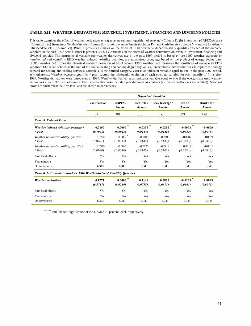
alternative channels in Table XII.
Following the empirical methodology outlined before, we report both reduced-form
(Panel A) and 2SLS-IV estimates (Panel B), where the IVs are EDD weather exposure quartiles.
We investigate whether revenue, investments, financing, and dividend policies responded
differentially for firms in distinct weather quartiles and in response to weather derivative use.
The impact on revenue is presented in Table XII, Column I. We do not find systematic
evidence that revenue increased in a differential manner for weather exposed firms. Not
surprisingly, the IV estimates on the effect of weather derivatives on revenue are also
insignificant. Such results are inconsistent with the hypothesis that global warming or
deregulation may be driving the effects on value, as those factors would tend to affect revenue in
weather sensitive regions differentially.
25
Table XII, Column II examines the effect of risk management on the level of capital
expenditures relative to asset values (nuclear plant information is not available in COMPUSTAT
after 1994). The reduced form estimates of Panel A indicate that firms in quartile 4 increased
their investments by one percentage point of assets, which is significant at the five percent level.
The resulting IV estimates in Panel B show that weather derivatives led to a positive and
significant effect on investment. The IV estimate is 0.047, which is significant at the five percent
level. As before, the standard errors in the IV specifications are large.
The fact that investments respond to risk management is consistent with Froot,
Scharfstein, and Stein (1993). Higher investment is, however, potentially consistent with
overinvestment stories due to agency concerns. Yet, the fact that higher investment rates are tied
to increases in firm value, suggests that the former hypothesis may be more empirically relevant.
The risk management consequences for financing decisions are investigated in Table XII,
Columns III (net debt), IV (book leverage), and V (cash to assets). Irrespective of the measure
used, reduced form estimates (Panel A) indicate that quartile 4 firms increase their reliance on
debt financing after 1997. Book leverage increases by 2.85 percentage points and cash to assets
declines 0.73 percentage points. The combined effect on net debt is 3.58, which is significant at
the five percent level. Consistent with tradeoff theories of capital structure, we find that weather
exposed firms were, as a result, able to use more debt and hold less cash than prior to 1997.
The IV estimates on the effect of weather derivatives in Table XII, Panel B reflect the
same signs as the reduced form correlations in Panel A. However, the standard errors are large
and, as a result, the effect of weather hedging on net debt and book leverage is only significant at
the 12 and 19 percent level, respectively. Despite the increased noise in the IV estimates, Column
V shows that hedging led to lower cash holdings. The estimated coefficient is -2.66, significant at
the 10 percent level.
An alternative test for the effect of risk management on leverage is to test in the cross-
section whether weather risk characteristics matter for capital structure after 1997. In unreported
results, we find that the across group differences in leverage, such as those reported in Table VI,
are no longer statistically different from zero at conventional levels after 1997. Lastly, Table XII,
Column VI examines the effect of weather derivatives on dividend ratios. We do not find
evidence that hedging led to significant effects on dividend decisions.
26
VII. CONCLUSIONS
Financial derivatives lie at the heart of Miller’s (1986) “revolution” in financial
innovation. Derivatives are increasingly important and controversial securities. They are powerful
tools for shifting or hedging risks. On the other hand, they also reduce the cost of engaging in
speculative transactions. The controversial feature of derivatives is exacerbated by their
prominent role in recent financial crises. Yet, establishing the risk management benefits of
financial derivatives is empirically difficult.
This paper provides direct evidence of the insurance benefits of financial derivatives on
firms’ valuation and financial policies. We seek to overcome the empirical challenges faced when
determining whether agents are hedging or speculating with derivatives by using a financial
innovation approach. More specifically, we use the introduction of weather derivatives as an
exogenous source of variation to firms’ hedging costs. To further identify the effect of weather
derivatives, we exploit variation in weather exposure prior to the introduction of these financial
contracts. Intuitively, we anticipate that those firms whose cash flows have historically fluctuated
with changing weather conditions are, relative to other firms, more likely to benefit from the
insurance feature of these contracts.
Using data from U.S. electric and gas utilities, two highly weather-sensitive sectors, we
find four main results. First, in the absence of weather derivatives, weather-exposed firms exhibit
significantly lower valuations and pursue more conservative operating and financing policies than
other firms. Second, measures of weather exposure that predate the introduction of weather
derivatives are strong predictors of weather derivative use upon innovation. Third, weather
derivatives led to a substantial increase in firm value. Fourth, hedging allows firms to increase
investment and to use more aggressive financing structures.
Overall, our results demonstrate that financial innovation that is targeted to meaningful
economic risks can significantly affect firm decisions. Our empirical approach isolates the use of
derivatives as risk management instruments. As a result, we show that hedging allows firms to
overcome market frictions, and that investment and financing policies respond to low cash flow
realizations.
Finally, whether our results extend to other industries or to alternative financial products
are fascinating areas for further research.
27
References
Adam, Tim R., and Chitru S. Fernando. 2006. “Hedging, Speculation, and Shareholder Value,”
Journal of Financial Economics 81:283–309. Adam, Tim, Sudipto Dasgupta, and Sheridan Titman. 2007. “Financial Constraints, Competition,
and Hedging in Industry Equilibrium,” Journal of Finance 62:2445–2473. Allayannis, George, and James P. Weston. 2001. “The Use of Foreign Currency Derivatives and
Firm Market Value,” Review of Financial Studies 14:243–276. Angrist, Joshua D., and Alan B. Krueger, “Instrumental Variables and the Search for
Identification: From Supply and Demand to Natural Experiments,” Journal of Economic Perspectives, 15 (2001), 69–85.
Arrow, Kenneth J. 1965. “Insurance Risk and Resource Allocation,” in Kenneth J. Arrow, Aspects of the Theory of Risk Bearing, Helsinki: Helsinki, Yrjo Jahnsson Lectures.
Bartram, Sohnke, Gregory, W. Brown, and Jennifer Conrad. 2009. “The Effects of Derivatives on Firm Risk and Value,” Working paper, University of North Carolina at Chapel Hill.
Bernstein, Peter L. 1996. Against the Gods: The Remarkable Story of Risk, John Wiley & Sons, New York.
Berrospide, Jose M., Amiyatosh Purnanandam, and Uday Rajan. 2007. “Corporate Hedging, Investment, and Value,” Working paper, University of Michigan.
Bodnar, Gordon M., Gregory S. Hayt, and Richard C. Marston. 1996. “Wharton Survey of Derivatives Usage by US Non-Financial Firms,” Financial Management 25:113–133.
Brockett, Patrick L., Mulong Wang, and Chuanhou Yang. 2005. “Weather Derivatives and Weather Risk Management,” Risk Management and Insurance Review, 8(1):127–140.
Carter, David, Daniel A. Rogers, and Betty J. Simkins. 2006. “Does Hedging Affect Firm Value? Evidence from the U.S. Airline Industry,” Financial Management 35:53–87.
Chance, Don M. 1998. Essays in Derivatives, John Wiley & SonsNew York. Chicago Mercantile Exchange. 2005. “An Introduction to CME Weather Products,” CME
Alternative Investment Products, http://www.cme.com. Conrad, Jennifer. 1989. “The Price Effect of Option Introduction,” The Journal of Finance44(2):
487–498. Considine, Geoffrey. 2000. “Introduction to Weather Derivatives.” Aquila Energy,
http://www.cmegroup.com/trading/weather/files/WEA_intro_to_weather_der.pdf. Cornaggia, Jess. 2010. “Does Risk Management Improve Productivity? Evidence from the U.S.
May 11. DeMarzo, Peter, M. and Darrell Duffie. 1995. “Corporate Incentives for Hedge and Hedge
Accounting.” Review of Financial Studies 8(3): 743–771. Dow Jones News Service. 1994. “Dominion Resources 1Q,” April 15. Economist (The). 2003. “A Hedge against the Heat,” August 16. Einstein, Albert. 1941. “Science and Religion” in Albert Einstein, Out of My Later Years, New
York, Philosophical Library, 21–30. Energy Information Administration. 2002. Derivatives and Risk Management in the Petroleum,
Natural Gas, and Electricity Industries, www.eia.gov. Energy Information Administration. 2003. Status of Electric Industry Restructuring Activity.
www.eia.gov. Fabrizio, Kira R., Nancy L. Rose, and Catherine D. Wolfram. 2007. “Do Markets Reduce Costs?
Assessing the Impact of Regulatory Restructuring on US Electric Generation Efficiency,” American Economic Review 97:1250–1277.
28
Froot, Kenneth A., David S. Scharfstein, and Jeremy C. Stein. 1993. “Risk Management: Coordinating Corporate Investment and Financing Policies,” Journal of Finance 48:1629–1658.
Garman, Mark, Carlos Blanco, and Robert Erickson. 2000. “Weather Derivatives: Instruments and Pricing Issues”, Financial Engineering Associates.
Géczy, Christopher, Bernadette A. Minton, and Catherine Schrand. 1997. “Why Firms Use Currency Derivatives,” The Journal of Finance 52(4):1323–1354.
Géczy, Christopher, Bernadette A. Minton, and Catherine Schrand. 2006. “The Use of Multiple Risk Management Strategies: Evidence from the Natural Gas Industry.” The Journal of Risk 8(3): 1–21.
Géczy, Christopher, Bernadette A. Minton, and Catherine Schrand. 2007. “Taking a View: Corporate Speculation, Governance and Compensation.” The Journal of Finance 62(5):2405–2443.
Goff, John. 2005. “Who’ll Stop the Rain?” CFO Magazine, April 1. Graham, John R., and Daniel A. Rogers. 2002. “Do Firms Hedge in Response to Tax Incentives?”
Journal of Finance 70:423–461. Guay, Wayne, and S. P. Kothari. 2003. “How Much Do Firms Hedge with Derivatives?” Journal
of Financial Economics 70:423–461. Haushalter, G. David. 2000. “Financing Policy, Basis Risk, and Corporate Hedging: Evidence
from Oil and Gas Producers,” The Journal of Finance 55: 107–152. Houston Chronicle. 1997. “Enron Contract Hedges Against Weather,” November 7. Jin, Yanbo, and Philippe Jorion. 2006. “Firm Value and Hedging: Evidence from U.S. Oil and
Gas Producers,” Journal of Finance 61:893–919. Leland, Hayne, E. 1998. “Agency Costs, Risk Management, and Capital Structure.” Journal of
Finance 53(4):1213–1243. MacKay, Peter, and Sara B. Moeller. 2007. “The Value of Corporate Risk Management,” Journal
of Finance 62:1379–1419. Markowitz, Harry M. 1952. “Portfolio Selection,” Journal of Finance 7:77–91. Mayers, David, and Clifford W. Smith, Jr. 1982 “On the Corporate Demand for Insurance,”
Journal of Business 55(2):281–296. Miller, Merton. 1986. “Financial Innovation: The Last Twenty Years and the Next,” Journal of
Financial and Quantitative Analysis 4:459–471. Modigliani, Franco, and Merton H. Miller. 1958. The Cost of Capital, Corporation Finance and
the Theory of Investment,” American Economic Review 48:261–297. Nance, Deana R., Clifford W. Smith, Jr., and Charles W. Smithson. 1993. “On the Determinants
of Corporate Hedging,” Journal of Finance 48:267–284. National Research Council. 2003. Fair Weather: Effective Partnerships in the Weather and
Climate Services. National Academies Press, Washington D.C. Office of the Comptroller of the Currency (The). 2007. OCC’s Quarterly Report on Bank Trading
and Derivatives Activities, Fourth Quarter. U.S. Department of the Treasury, Washington, DC.
Omaha World-Herald (The). 992 “Utility: Cool Weather Is Why Earnings Fell,” November 3. Roll, Richard. 1984. “Orange Juice and Weather,” American Economic Review 74:861–880. Skapinker, Michael. 2003, “Whatever the Weather, It’s No Excuse to Lose Money,” Financial
Times, September, 17. Smith, Clifford W., and Rene Stulz. 1985. “The Determinants of Firms’ Hedging Policies,”
Journal of Financial and Quantitative Analysis 28:391–405. Stulz, René M. 1984. “Optimal Hedging Policies,” Journal of Financial and Quantitative
Analysis 19:127–140. Stulz, René M. 2003. Risk Management and Derivatives, Thomson South-Western, Mason, Ohio.
29
Stulz, René. M. 2004. “Should We Fear Derivatives?” Journal of Economic Perspectives, 18(3): 173–192.
Swan, Edward J. 2000. Building the Global Market: a 4000 Year History of Derivatives, Kluwer Law International, Boston.
Tobin, James. 1969. "A General Equilibrium Approach to Monetary Theory." Journal of Money Credit and Banking 1(1):15–29.
Tufano, Peter. 1996. “Who Manages Risk? An Empirical Examination of Risk Management Practices in the Gold Mining Industry,” Journal of Finance 51:1097–1137.
Tufano, Peter. 1998. “The Determinants of Stock Price Exposure: Financial Engineering and the Gold Mining Industry,” Journal of Finance 53:1015–1052.
Tufano, Peter. 2003. “Financial Innovation,” in George M. Constantinides and Milton Harris & Rene M. Stulz (eds.), Handbook of the Economics of Finance, edition 1, volume 1, chapter 6, 307–335, Elsevier.
Utley, Michael. 1998. “FPL Income Soars with the Heat,” The Palm Beach Post, July 16. Vincenty, Thaddeus. 1975, “Direct and Inverse Solutions of Geodesics on the Ellipsoid with
Application of Nested Equations, Survey Review 23(176): 88–93. Weather Risk Management Association. 2005. “Results for the Annual Industry Survey,”
TABLE I. SUMMARY STATISTICS This table shows summary statistics for 203 U.S. electric and gas firms (SIC codes 4911, 4923, 4924, 4931, and 4932) with matching (a) financial information from COMPUSTAT for at least 10 years prior to 1997 and (b) weather data from the National Oceanic and Atmospheric Administration (NOAA). Panel A. presents financial and weather variables. Total assets, revenue, and market value of equity are in thousands of constant 2008 dollars (Consumer Price Index, adjusted, 2008=100). OROA is the ratio of operating income before depreciation to assets. Book leverage / assets is the ratio of the sum of long-term debt plus existing debt in current liabilities to total assets. Market value of equity is the price (close) times the number of common shares outstanding. M-B ratio or market-to-book ratio is the book value of assets plus market value of common equity minus book value of common equity and deferred taxes divided by total assets. Net debt / assets is the ratio of book leverage minus cash and marketable securities to total assets. CAPEX / assets is the ratio of capital expenditures to total assets. Investment rate is the growth rate of total assets. Nuclear plant generation is an indicator variable equal to one if a utility has nuclear-powered generating plants, zero otherwise. Common dividends / assets is the ratio of common dividends over total assets. Weather variables reported are cooling, heating and energy degree days. A heating (cooling) degree day reflects the number of degrees that a daily average temperature is below (above) 65°F, zero otherwise. Energy degree days are the sum of heating and cooling degree days. Cooling, heating, and energy degree days seek to capture cooling, heating, and cooling and heating energy demand, respectively. Heating (cooling) degree days, annual is sum of daily heating (cooling) degree days in a year in the firms’ main location. In Panel B, weather (natural gas, interest derivative) user is an indicator variable equal to one if a firm used weather, natural gas, or interest rate derivatives in the post-1997 period, zero otherwise.
Panel A. Firm and Weather Information
Variables Number Obs Mean Std Dev. Min p10 Median p90 Max
Total assets 8,161 5,152 6,723 62 500 2,702 13,662 73,370
TABLE II. WEATHER SHOCKS AND OPERATING PERFORMANCE
This table presents the impact of mild temperatures (low energy degree days (EDDs)) on measures of operating performance. The dependent variables are (a) ln revenue, the natural logarithm of revenue in constant 2008 dollars (Column I), (b) OROA, the operating profitability on assets (Column II), (c) ln operating income, the natural logarithm of operating income in constant dollars (Column III), (d) dividends/assets, the ratio of common stock dividends to assets (Column IV), and (e) investment rate, the growth rate of total assets (Column V). EDDs are defined as the sum of the annual heating and cooling degree day values, temperatures indexes that seek to capture the energy demand for heating and cooling services. Heating (cooling) degree days reflects the number of degrees that a daily average temperature is below (above) 65°F. Weather shock is an indicator variable equal to one if the annual EDD values are in the lowest quintile for each sample firm, zero otherwise. Each column shows the results of a fixed-effects (firm) regression that also includes the natural logarithm of lagged total assets and year dummies as controls (estimated coefficients are omitted). Standard errors are clustered at the firm level and are shown in parentheses.
***, ** and * denote significance at the 1, 5 and 10 percent level, respectively.
TABLE III. MEASURES OF WEATHER EXPOSURE This table shows summary statistics (Panel A) and correlations (Panel B) of various measures of weather exposure. Risk measures include (a) revenue volatility (standard deviation of quarterly revenue to assets), (b) CDD, HDD, and EDD betas (absolute value of the estimated coefficient of CDD, HDD, and EDD, respectively, on quarterly revenue to assets) or “weather betas”, (c) CDD, HDD, and EDD historical standard deviation, and (d) CDD, HDD, and EDD weather induced volatility, which is the product of CDD, HDD, and EDD weather betas times their relevant historical standard deviation. All measures are estimated using pre-1997 data.
TABLE IV. REVENUE CONSEQUENCES OF WEATHER SHOCKS: BY MEASURES OF WEATHER
EXPOSURE This table presents the impact of mild temperatures (low energy degree days (EDDs)) on the revenue of firms sorted by their estimated weather exposure. The dependent variable is ln revenue, the natural logarithm of revenue in constant 2008 dollars. EDDs are defined as the sum of the annual heating and cooling degree day values, temperatures indexes that seek to capture the energy demand for heating and cooling services. Heating (cooling) degree days reflects the number of degrees that a daily average temperature is below (above) 65°F. Weather shock is an indicator variable equal to one if the annual EDD values are in the lowest quintile for each firm, zero otherwise. Measures of weather exposure are (a) Revenue / Assets quartiles, equal-sized groupings based on the historical standard deviation of quarterly revenue divided by assets (Column I), (b) weather beta quartiles, equal sized-groupings based on the absolute value of the sensitivity of revenue to CDD (Column II), HDD (Column III), and EDD (Column IV) values, and (c) weather induced volatility quartiles, equal-sized groupings based on the product of CDD (Column V), HDD (Column VI), and EDD (Column VII) weather betas, respectively and their historical standard deviation. Each column shows the results of a fixed-effects (firm) regression that also includes the natural logarithm of lagged total assets and year dummies as controls (estimated coefficients are omitted). Standard errors are clustered at the firm level and are shown in parentheses.
***, ** and * denote significance at the 1, 5 and 10 percent level, respectively.
TABLE V. WEATHER EXPOSURE AND MARKET VALUATION BEFORE 1997
This table examines the impact of weather risk exposure on firm value before weather derivatives were introduced. Weather exposure is measured using, alternatively, (a) Revenue / Assets quartiles, equal-sized groupings based on the historical standard deviation of quarterly revenue divided by assets (Columns I to IV, and VII), (b) weather induced volatility quartiles, equal-sized groupings based on the product of energy degree days (EDD) weather beta times the historical standard deviation of EDD values (Columns V, VI, and VIII). EDD weather beta measures the sensitivity of revenue to EDD variation. EDDs are defined as the sum of the annual heating and cooling degree day values, temperatures indexes that seek to capture the energy demand for heating and cooling services. The dependent variables are the market-to-book ratio (Columns I-VI) and the natural logarithm of market value of equity (VII and VIII). Market-to-book is defined as the value of total assets plus the market value of common equity (stock price times the number of common shares outstanding) minus book value of common equity and deferred taxes divided by total assets. Market value of equity is the price (close) times the number of common shares outstanding. Other controls include: Ln assets, the natural logarithm of total assets; OROA, the ratio of operating income to total assets; Investment rate, the rate of growth of total assets. Standard errors are clustered at the firm level and are shown in parentheses.
***, ** and * denote significance at the 1, 5 and 10 percent level, respectively.
Variables (I) (II) (III) (IV) (V) (VI) (VII) (VIII)
Market to Book Ratio, pre- 1997 Ln Market Value, pre-1997
35
TABLE VI. WEATHER EXPOSURE, AND INVESTMENT AND FINANCIAL DECISIONS BEFORE 1997
This table examines the impact of weather exposure on investment, production choice, financing, and dividend policies before weather derivatives were introduced. The dependent variables are (a) CAPEX / Assets: the ratio of capital expenditures to total assets (Columns I and II), (b) Nuclear Plant Generation: an indicator variable equal to one if a utility has nuclear-powered generating plants, zero otherwise (Columns III and IV), (c) Net Debt / Assets: is the ratio of the book value of debt minus cash and marketable securities over total assets (Columns V and VI), and (d) Dividend / Assets: is the ratio of common dividends over total assets (Columns VII and VIII). Weather exposure is measured using, alternatively, (i) Revenue / Assets quartiles (Columns I, III, V, and VII), equal-sized groupings based on the historical standard deviation of quarterly revenue divided by assets, (ii) EDD weather induced volatility quartiles (Columns II, IV, VI, VIII), equal-sized groupings based on the product of energy degree days (EDD) weather beta times the historical standard deviation of EDD values. EDD weather beta measures the sensitivity of revenue to EDD variation. EDDs are defined as the sum of the annual heating and cooling degree day values, temperatures indexes that seek to capture the energy demand for heating and cooling services. Ln assets is the natural logarithm of total assets. OROA is the ratio of operating income to total assets. M-B ratio is defined as the value of total assets plus the market value of common equity (stock price times the number of common shares outstanding) minus book value of common equity and deferred taxes divided by total assets. Columns I, II, and V to VIII are linear specifications, and Columns III and IV are probit models. Each regression also includes state and year dummies as controls (estimated coefficients are omitted). Standard errors are clustered at the firm level and are shown in parentheses.
***, ** and * denote significance at the 1, 5 and 10 percent level, respectively.
TABLE VII. DERIVATIVE USE AND FIRM VALUE AROUND 1997 This table presents the impact of financial derivatives on firm value. The dependent variables are (a) the market-to-book ratio (Columns I to VI) and (b) the natural logarithm of market value of equity (Column VII). Market-to-book is defined as the value of total assets plus the market value of common equity (stock price times the number of common shares outstanding) minus book value of common equity and deferred taxes divided by total assets. Market value of equity is the price (close) times the number of common shares outstanding. Weather (interest rate, natural gas) derivative is an indicator variable equal to one if a firm used weather (interest rate, natural gas) derivatives after 1997, and zero otherwise. Post is an indicator variable equal to one in the post-1997 period, zero otherwise. Ln assets is the natural logarithm of total assets. OROA is the ratio of operating income to total assets. Investment rate is the growth rate of total assets. Each specification also includes year dummies as controls (estimated coefficients are omitted). Standard errors are clustered at the firm level and are shown in parentheses.
***, ** and * denote significance at the 1, 5 and 10 percent level, respectively.
Variables (I) (II) (III) (IV) (V) (VI) (VII)
Weather derivatives * post 0.0523**
0.0540**
0.0463*
0.0482*
0.1203**
(0.0259) (0.0258) (0.0264) (0.0262) (0.0593)
Interest rate derivatives * post -0.0089 -0.0176 -0.0279 -0.1240 **
(0.0396) (0.0395) (0.0401) (0.0594)
Natural gas derivatives * post 0.0397 * 0.0324 0.0365 0.0991 *
TABLE VIII. WEATHER EXPOSURE AND FIRM VALUE (“REDUCED FORM”) This table reports post-1997 valuation effects as a function of alternative measures of pre-1997 weather exposure. The dependent variable is the market-to-book ratio, the value of total assets plus the market value of common equity minus book value of common equity and deferred taxes divided by total assets. Measures of weather exposure are (a) Revenue / Assets quartiles (Column I), equal-sized groupings based on the historical standard deviation of quarterly revenue divided by assets, (b) EDD (Column II), CDD (Column III), and HDD (Column IV) weather induced volatility quartiles, equal-sized groupings based on the product of energy, cooling and heating degree days (EDD, HDD, and CDD, respectively) weather beta times the historical standard deviation of each of those variables. EDD, HDD, and CDD weather betas measure the sensitivity of revenue to EDD, HDD, and CDD variation, respectively. EDDs are defined as the sum of the annual heating and cooling degree day values, temperatures indexes that seek to capture the energy demand for heating and cooling services. (c) | | significant, is an indicator variable equal to one if the EDD weather beta is statistically significant at the five-percent level, zero otherwise (Column V). Post is an indicator variable equal to one in the post-1997 period, zero otherwise. Ln assets is the natural logarithm of total assets. OROA is the ratio of operating income to total assets. Investment rate is the growth rate of total assets. Each specification also includes year dummies as controls (estimated coefficients are omitted). Standard errors are clustered at the firm level and are shown in parentheses.
***, ** and * denote significance at the 1, 5 and 10 percent level, respectively.
Variables (I) (II) (III) (IV) (V)
Weather-Based Quantity Risk 0.1079***
0.1044***
0.1317***
0.1002***
Quartile 4 * Post (0.0324) (0.0303) (0.0290) (0.0348)
TABLE IX. WEATHER EXPOSURE AND WEATHER DERIVATIVE USE (FIRST STAGE) This table examines the effect of pre-1997 weather exposure measures on post-1997 weather derivative use. The dependent variable is weather derivative use, an indicator variable equal to one if a firm used weather derivatives in the post-1997 period, zero otherwise. Measures of weather exposure are (a) Revenue / Assets quartiles (Column I), equal-sized groupings based on the historical standard deviation of quarterly revenue divided by assets, (b) EDD (Column II), CDD (Column III), and HDD (Column IV) weather induced volatility quartiles, equal-sized groupings based on the product of energy, cooling and heating degree days (EDD, HDD, and CDD, respectively) weather beta times the historical standard deviation of each of those variables. EDD, HDD, and CDD weather betas measure the sensitivity of revenue to EDD, HDD, and CDD variation, respectively. EDDs are defined as the sum of the annual heating and cooling degree day values, temperatures indexes that seek to capture the energy demand for heating and cooling services. (c) | | significant, is an indicator equal to one if the EDD weather beta is statistically significant at the five-percent level, zero otherwise (Column V). Post is an indicator variable equal to one in the post-1997 period, zero otherwise. Standard errors are clustered at the firm level and are shown in parentheses.
***, ** and * denote significance at the 1, 5 and 10 percent level, respectively.
Variables
Weather-Based Quantity Risk 0.2175**
0.2201***
0.2163**
0.1820**
Quartile 4 * Post (0.0855) (0.0842) (0.0847) (0.0839)
TABLE X. WEATHER DERIVATIVES AND FIRM VALUE (2SLS) This table presents 2SLS-IV estimates on the impact of weather derivatives on firm value. The dependent variable is the market-to-book ratio. Market-to-book ratios are defined as the value of total assets plus the market value of common equity (stock price times the number of common shares outstanding) minus book value of common equity and deferred taxes divided by total assets. Weather derivatives, is an indicator variable equal to one if a firm used weather derivatives in the post-1997 period, zero otherwise. The instruments for weather derivatives are based on measures of pre-1997 weather exposure, and are, alternatively: (a) EDD weather induced volatility quartiles (Columns I and II), equal-sized groupings based on the product of energy degree days (EDD) weather beta times the historical standard deviation of EDD values. EDD weather beta measures the sensitivity of revenue to EDD variation. EDDs are defined as the sum of the annual heating and cooling degree day values, temperatures indexes that seek to capture the energy demand for heating and cooling services. (b) Revenue / Assets quartiles (Columns III and IV), equal-sized groupings based on the historical standard deviation of quarterly revenue divided by assets. (c) | | significant (Columns V and VI), an indicator equal to one if the EDD weather beta is statistically significant at the five-percent level, zero otherwise. Weather derivatives were introduced in 1997. Ln assets is the natural logarithm of total assets. OROA is the ratio of operating income to total assets. Investment rate is the growth rate of total assets. Each specification also includes year dummies as controls (estimated coefficients are omitted). Standard errors are clustered at the firm level and are shown in parentheses.
***, ** and * denote significance at the 1, 5 and 10 percent level, respectively.
Dependent Variable: Market to Book Ratio, Post 1997
Instrumental Variables
EDD Weather Induced
Volatility
40
TABLE XI. WEATHER DERIVATIVES AND FIRM VALUE (2SLS): ALTERNATIVE HYPOTHESES This table presents 2SLS-IV estimates on the impact of weather derivatives on firm value. The dependent variable is the market-to-book ratio. Market-to-book ratios are defined as the value of total assets plus the market value of common equity (stock price times the number of common shares outstanding) minus book value of common equity and deferred taxes divided by total assets. Weather derivatives, is an indicator variable equal to one if a firm used weather derivatives in the post-1997 period, zero otherwise. The instrumental variable for weather derivatives use in the post-1997 period is based on pre-1997 weather exposure or weather induced volatility. EDD weather induced volatility quartiles, are equal-sized groupings based on the product of energy degree days (EDD) weather beta times the historical standard deviation of EDD values. EDD weather beta measures the sensitivity of revenue to EDD variation. EDDs are defined as the sum of the annual heating and cooling degree day values, temperatures indexes that seek to capture the energy demand for heating and cooling services. Weather derivatives were introduced in 1997. Ln CDD (Ln HDD) is the natural logarithm of CDD (HDD). Deregulation electricity (natural gas) is an indicator variable equal to one for the observations where the relevant state-year has experienced deregulation in electricity (natural gas) markets, respectively, zero otherwise. Deregulation access to retail, industry and all consumers are indicator variables equal to one for the observations where the relevant state-year has experienced deregulation to access to retail, industry and all consumers, respectively, and zero otherwise. Dereg. NG pilot, partial and all consumers are indicator variables equal to one for the observations where the relevant state-year has experienced natural gas deregulation for pilot, partial and all consumers, respectively, and zero otherwise. Interest rate (natural gas) derivatives is an indicator variables equal to one if a firm used interest rate (natural gas) derivatives in the post-1997 period, zero otherwise. Ln assets is the natural logarithm of total assets. OROA is the ratio of operating income to total assets. Investment rate is the growth rate of total assets. Each specification also includes year dummies as controls (estimated coefficients are omitted). Standard errors are clustered at the firm level and are shown in parentheses.
***, ** and * denote significance at the 1, 5 and 10 percent level, respectively.
Variables (I) (II) (III) (IV) (V) (VI) (VII) (VIII)
TABLE XII. WEATHER DERIVATIVES: REVENUE, INVESTMENT, FINANCING AND DIVIDEND POLICIES This table examines the effect of weather derivatives on (a) revenue (natural logarithm of revenue) (Column I), (b) investment (CAPEX/Assets) (Column II), (c) financing (Net debt/Assets (Column III), Book Leverage/Assets (Column IV) and Cash/Assets (Column V)) and (d) Dividends (Dividend/Assets) (Column VI). Panel A presents estimates on the effect of EDD weather-induced volatility quartiles on each of the outcome variables in the post-1997 period. Panel B presents 2SLS-IV estimates on the effect of weather derivatives on revenue, investment, financing and dividend policies. The instrumental variable for weather derivatives use in the post-1997 period is based on pre-1997 weather exposure or weather induced volatility. EDD weather induced volatility quartiles, are equal-sized groupings based on the product of energy degree days (EDD) weather beta times the historical standard deviation of EDD values. EDD weather beta measures the sensitivity of revenue to EDD variation. EDDs are defined as the sum of the annual heating and cooling degree day values, temperatures indexes that seek to capture the energy demand for heating and cooling services. Quartile 1 is the omitted category. Post is an indicator variable equal to one in the post-1997 period, zero otherwise. Weather exposure quartiles * post, capture the differential evolution of each outcome variable for each quartile of firms after 1997. Weather derivatives were introduced in 1997. Weather derivatives is an indicator variable equal to one if the energy firm used weather derivatives after 1997, zero otherwise. Each specification also includes year dummies as controls (estimated coefficients are omitted). Standard errors are clustered at the firm level and are shown in parentheses.
***, ** and * denote significance at the 1, 5 and 10 percent level, respectively.
FIGURE 1. MONTHLY ELECTRICITY AND NATURAL GAS UNITS AND AVERAGE TEMPERATURES, 2005
Figure A shows the 2005 monthly electricity sales in the United States (thousands of gigawatts per hour or GWh) and the corresponding average monthly temperature (°F). Figure B shows the 2005 monthly natural gas sales in the United States (thousands of million cubic feet or MMcf) and the corresponding average monthly temperature (°F). Data on electricity and natural gas sales are from the Energy Information Administration (EIA), forms 826 and 857, respectively. Data on monthly temperatures are from the National Oceanic and Atmospheric Administration (NOAA).
A. Monthly Electricity Sales (Units: GWh) and Average Temperatures
B. Monthly Natural Gas Sales (Units: MMcf) and Average Temperatures
200
250
300
350
400
Jan Feb Mar Apr May Jun Jul Aug Sep Oct Nov Dec
0
20
40
60
80
100
Electricity (GWh) Temperature (°F)
Temperature (°F)1,000s (GWh)
1,000
1,500
2,000
2,500
3,000
Jan Feb Mar Apr May Jun Jul Aug Sep Oct Nov Dec
0
20
40
60
80
100
Natural Gas Sales Temperature (°F)
Temperature (°F)1,000s (MMcf)
43
FIGURE 2. MONTHLY ELECTRICITY AND NATURAL GAS UNITS, AND MONTHLY COOLING AND
HEATING DEGREE DAYS, 2005 Figure A shows the scaled (August sales=100) monthly electricity sales in the United States in 2005 (thousands of gigawatts per hour or GWh), and the monthly cooling degree days (CDD) (°F). Figure B shows the scaled (January sales=100) monthly natural gas sales in the United States (thousands of million cubic feet or MMcf) and the monthly heating degree days (HDD). Heating and cooling degree day values seek to capture the energy demand for heating and cooling services, respectively. A heating (cooling) degree day reflects the number of degrees that a daily average temperature is below (above) 65° F. Data on electricity and natural gas sales are from the Energy Information Administration (EIA), forms 826 and 857, respectively. CDD and HDD data are from the National Oceanic and Atmospheric Administration (NOAA).
A. Monthly Electricity Sales (Scaled, August=100), and Cooling Degree Days
B. Monthly Natural Gas Sales (Scaled, Jan=100), and Heating Degree Days
70
75
80
85
90
95
100
105
Jan Feb Mar Apr May Jun Jul Aug Sep Oct Nov Dec
0
50
100
150
200
250
300
350
Scaled Electricity Sales Cooling Degree Days (°F)
Monthly Cooling Degree Days (°F)Scaled Electricity Sales (August Sales=100)
50
60
70
80
90
100
Jan Feb Mar Apr May Jun Jul Aug Sep Oct Nov Dec
0
200
400
600
800
1000
Scaled Natural Gas Sales Heating Degree Days (°F)
Monthly Heating Degree Days (°F)Scaled Natural Gas Sales (January Sales=100)
44
FIGURE 3. REGIONAL DIFFERENCES IN ENERGY VOLUME VARIATION, 2005 Figure A shows the scaled (March sales=100) monthly electricity sales in Louisiana and Montana in 2005 (thousands of gigawatts per hour or GWh). Figure B shows the scaled (March sales=100) monthly natural gas sales in Louisiana and Montana (thousands of million cubic feet or MMcf). Data on electricity and natural gas sales are from the Energy Information Administration (EIA), forms 826 and 895, respectively.
A. Monthly Electricity Sales (Scaled, March=100)
B. Monthly Natural Gas Sales (Scaled, March=100)
70
80
90
100
110
120
130
140
150
Jan Feb Mar Apr May Jun Jul Aug Sep Oct Nov Dec
California Louisiana Montana
Scaled Electricity Volumes (March Sales, GWh=100)
20
40
60
80
100
120
140
160
Jan Feb Mar Apr May Jun Jul Aug Sep Oct Nov Dec
California Louisiana Montana
Scaled Natural Gas Volumes (March Sales, MMcf =100)