SHRP-H-350 Road Weather Information Systems Volume 1: Research Report S. Edward Boselly III G. Stanley Doore The Matrix Management Group 811 1st Ave., Suite 466 Seattle, Washington 98104 Dr. John E. Thornes School of Geography University of Birmingham Birmingham, England B15 2TT Dr. Cyrus Ulberg Donald D. Ernst, P.E. The Washington Transportation Center (TRAC) University of Washington Seattle, Washington 98195 Strategic Highway Research Program National Research Council Washington, DC 1993 shrp
Transcript
SHRP-H-350
Road Weather Information SystemsVolume 1: Research Report
S. Edward Boselly IIIG. Stanley Doore
The Matrix Management Group811 1st Ave., Suite 466
Seattle, Washington 98104
Dr. John E. Thornes
School of GeographyUniversity of Birmingham
Birmingham, England B15 2TT
Dr. Cyrus UlbergDonald D. Ernst, P.E.
The Washington Transportation Center (TRAC)University of Washington
Seattle, Washington 98195
Strategic Highway Research ProgramNational Research Council
Program Manager: Don M. HarriottProject Manager: L. David MinskProgram Area Secretary: Francine BurgessCopy Editor: Katharyn Bine BrosseauProduction Editor: Cara J. Tate
September 1993
key words:highwaysice detectionmaintenance
meteorologypavement ice detectorsroad weather information systemssnow and ice control
weather forecasting
Strategic Highway Research ProgramNational Academy of Sciences2101 Constitution Avenue N.W.
Washington, DC 20418
(202) 334-3774
The publication of this report does not necessarily indicate approval or endorsement of the findings, opinions,conclusions, or recommendations either inferred or specifically expressed herein by the National Academy ofSciences, the United States Government, or the American Association of State Highway and TransportationOfficials or its member states.
The research described herein was supported by the Strategic Highway Research Program(SHRP). SHRP is a unit of the National Research Council that was authorized by section128 of the Surface Transportation and Uniform Relocation Assistance Act of 1987.
We wish to thank the state highway maintenance personnel who took the time to completethe detailed questionnaire, and the following states and province of Canada that consented toin-person interviews of snow and ice control staff:
•Massachusetts PennsylvaniaNew Jersey MichiganMinnesota Missouri
Colorado WyomingWashington AlaskaBritish Columbia Wisconsin
We wish to give additional thanks to the states that participated in our field test programduring the 1990-1991 winter:
Massachusetts New JerseyMichigan MinnesotaColorado Missouri
Washington
We relied on the vendors of road weather information system (RWIS) equipment forassistance in data gathering and formatting for our analysis. Special thanks go to SurfaceSystems Inc. (SSI), Climatronics, and Vaisala for providing data support. SSI also assistedwith a detailed investigation of the use of a hand-held radiometer for pavement temperaturecomparison measurements.
And special thanks must go to Mr. Ingmar Olofsson of SweRoad, a Swedish consulting firm,who served as an invaluable' source of information through the EUCO-COST 309international research project investigating road weather information systems.
Finally, we thank the meteorological equipment vendors and the private and governmentalmeteorological services providers who took their valuable time to complete questionnairesand to assist the project team.
iii
Contents
Acknowledgments ........................................... iii
List of Figures ............................................. ix
List of Tables ............................................. xi
1 Introduction ........................................... 7Statement of the Problem ................................... 7Standard Weather Information ................................ 9
Field Testing of Sensors .............................. 30Representativeness of Pavement Sensor Reports ........... 30Sensor Placement in the Roadway .................... 33Recommendations for Sensor Placement in the Roadway ...... 36Location of RPUs and Weather Sensors ................ 38Recommendations for Location of RPUs and Weather Sensors . . 40
Evaluation of Road Meteorology Sources ........................ 44Types of Meteorology Sources .......................... 44
Media ..................................... 44The National Weather Service ...................... 45Other Government Sources ........................ 46
Value-added Meteorological Services .................. 46Evaluation of Sources ................................ 47
Field Testing Results ................................ 47Uses of Meteorological Data ....................... 50Weather Forecasts ............................. 50
Pavement Temperature Forecasts .................... 53Conclusions ...................................... 53Recommendations .................................. 54
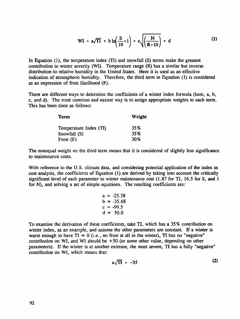
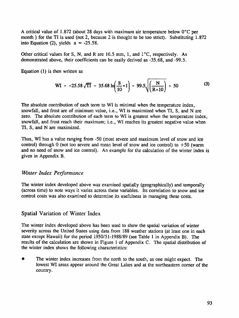
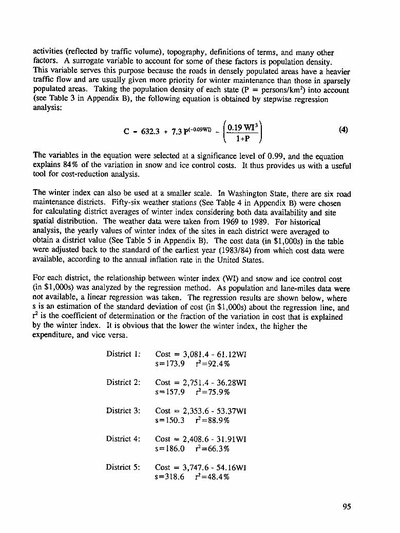
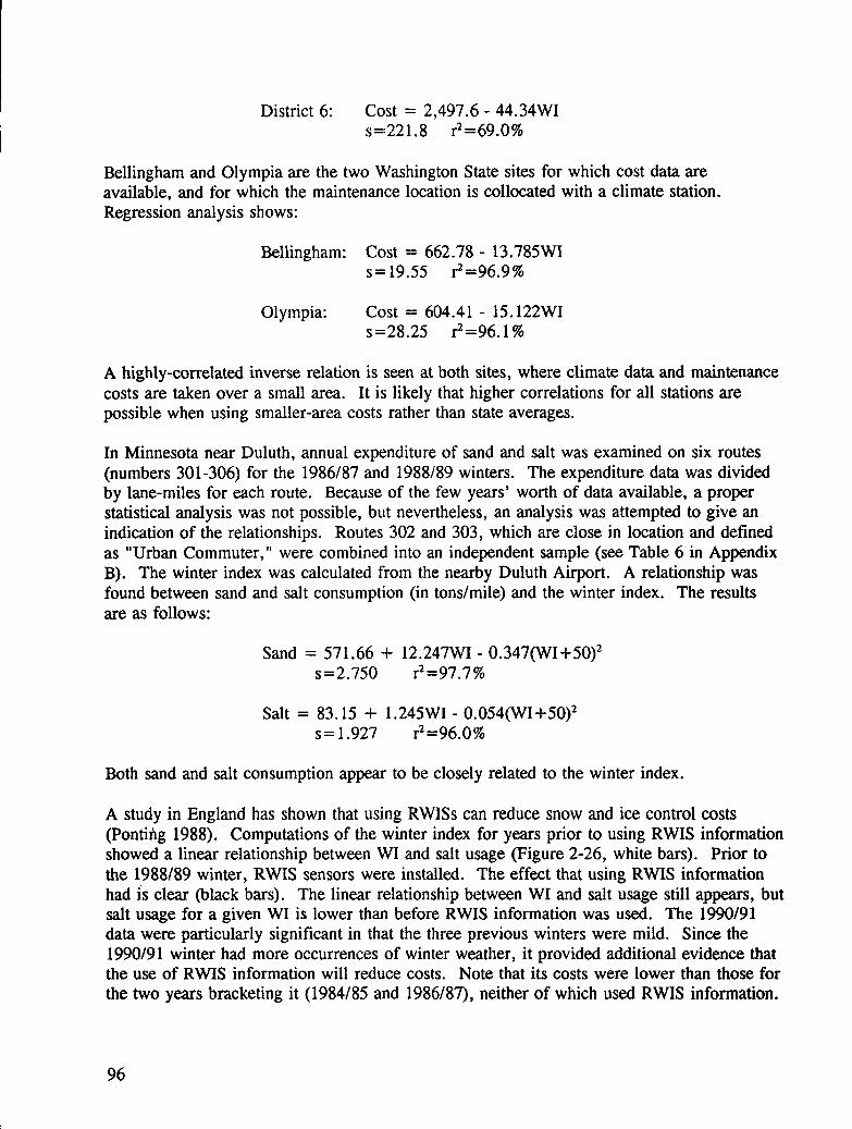
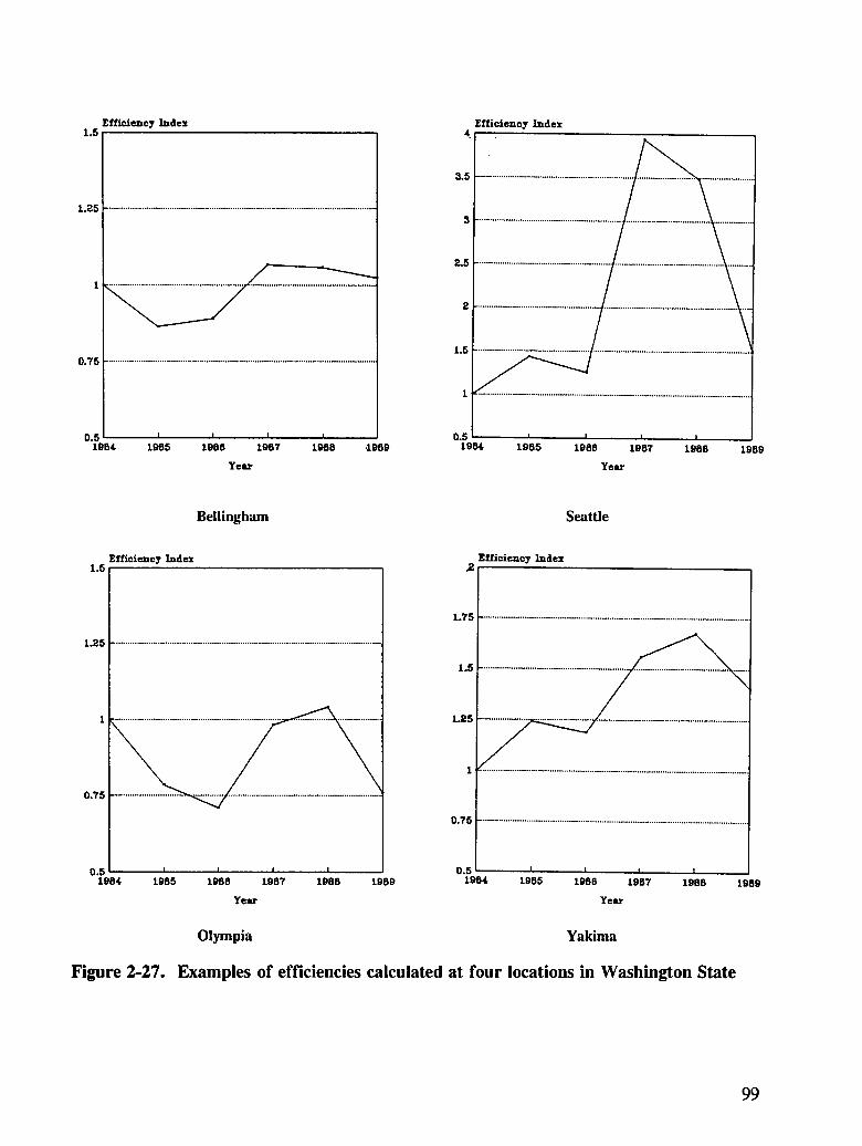
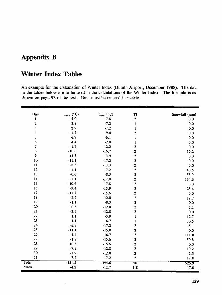
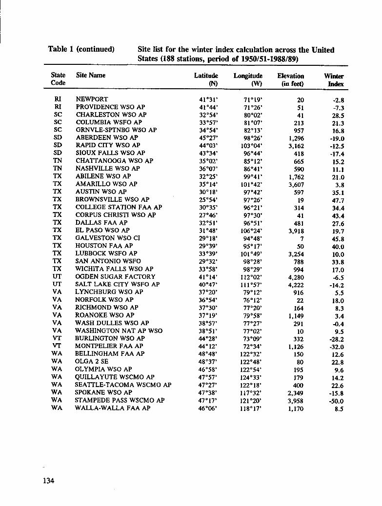
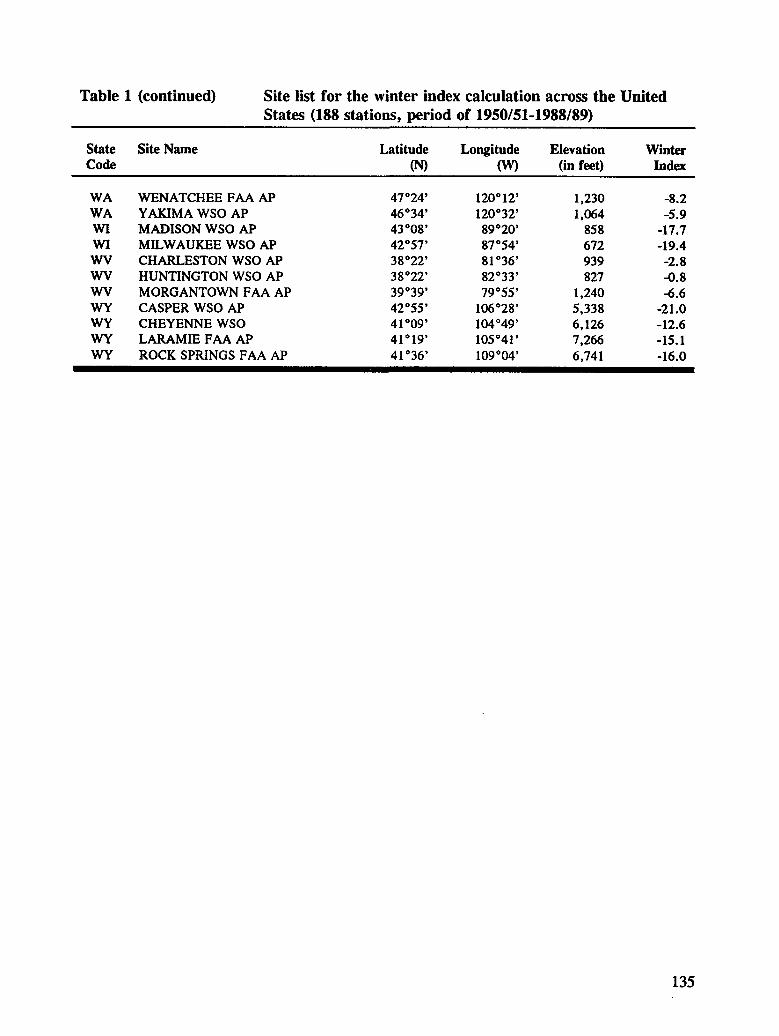
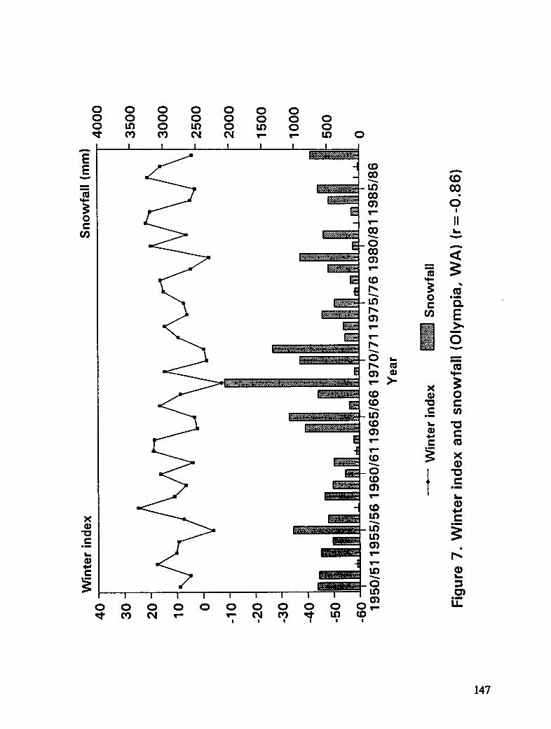
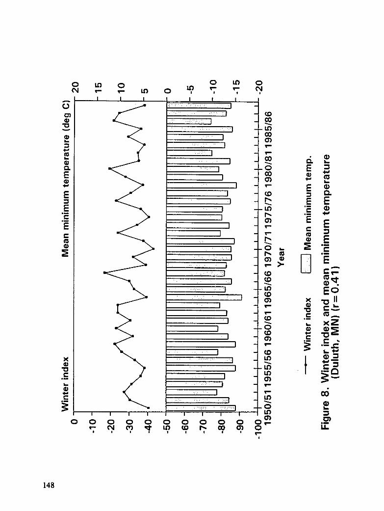
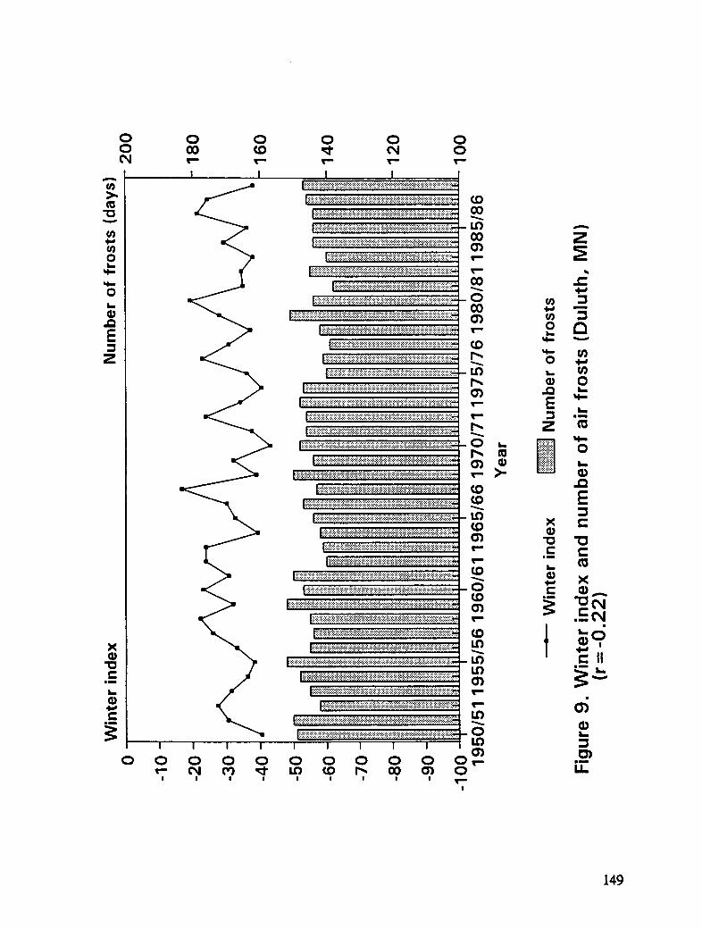
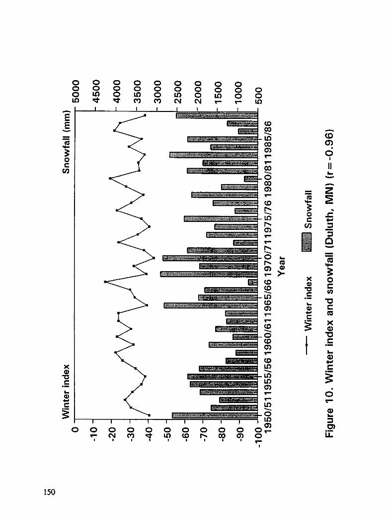
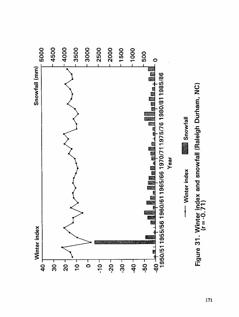
Winter Index ......................................... 90
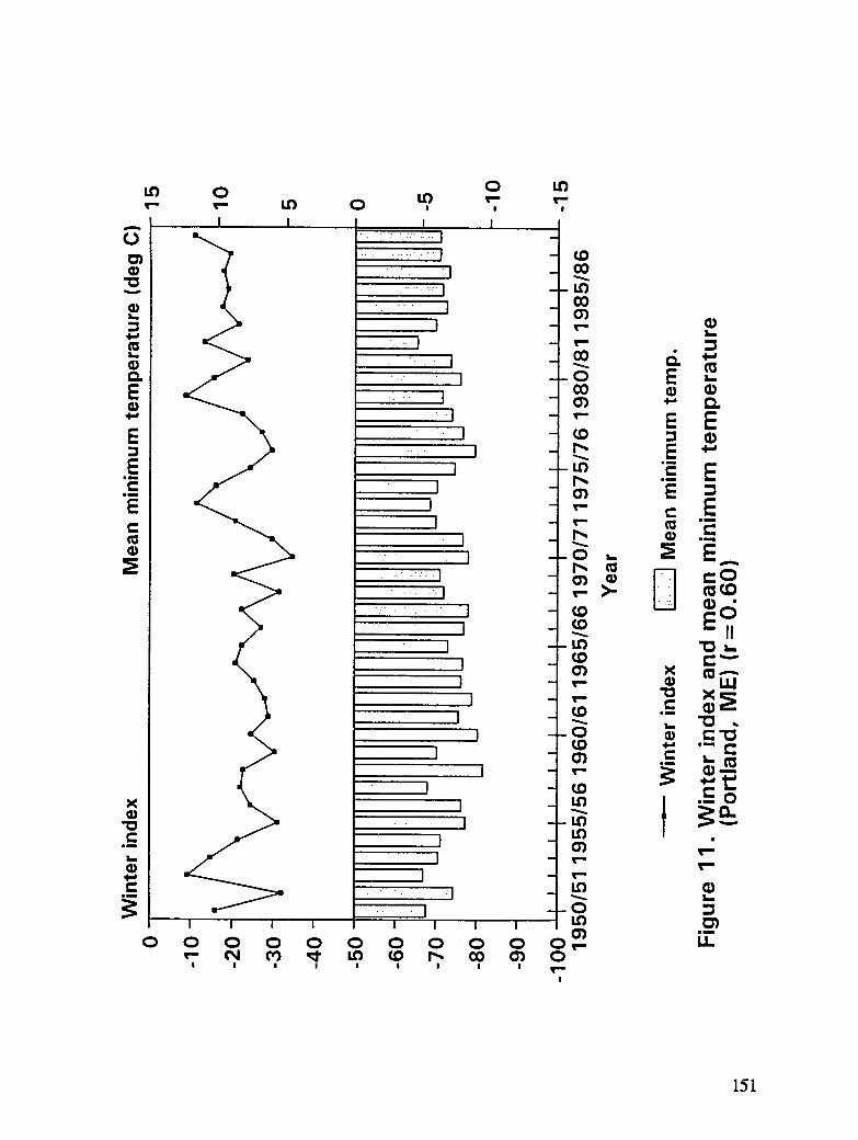
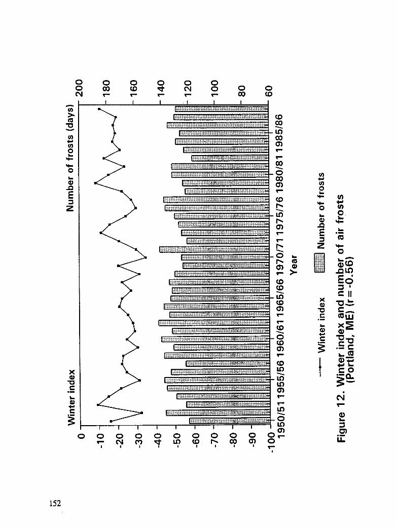
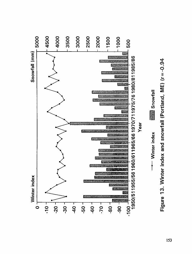
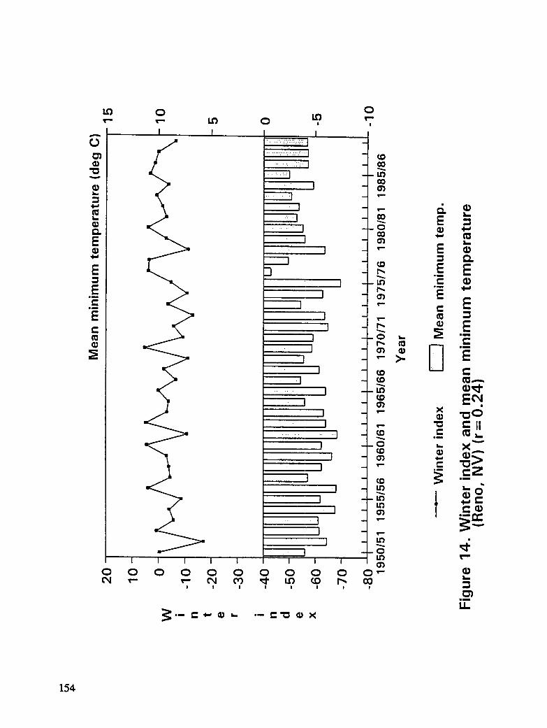
Purpose ........................................ 90Methodology ..................................... 91Winter Index Performance ............................. 93
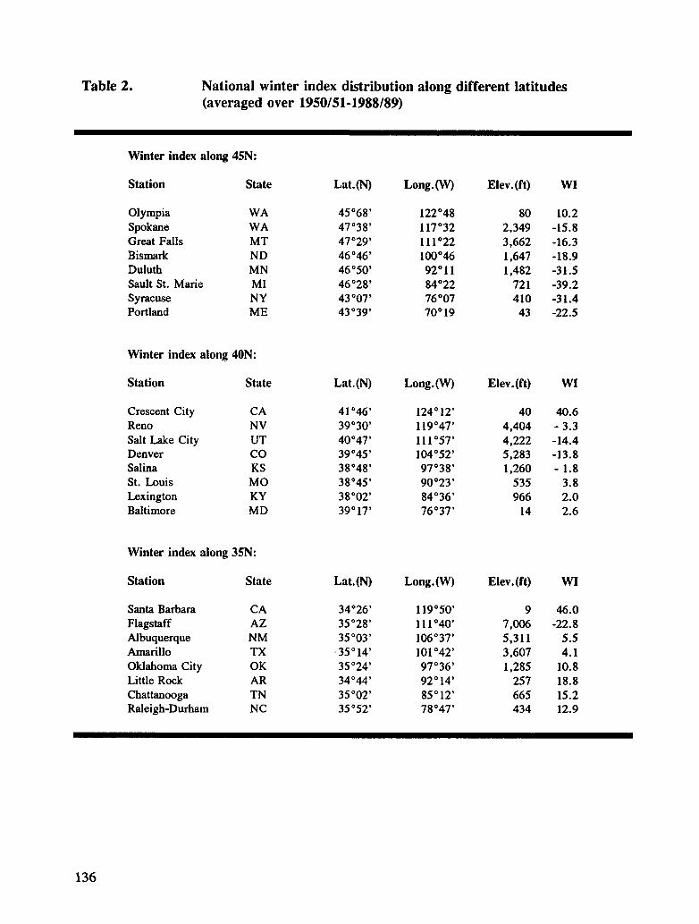
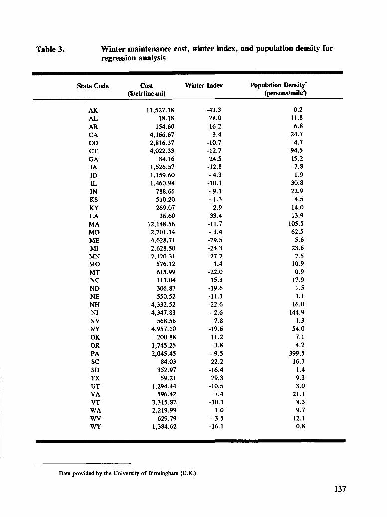
Spatial Variation of Winter Index .................... 93Temporal Variation of Winter Index .................. 94Correlation of Winter Index to Snow and Ice Control Costs .... 94
3 RWIS Implementation ................................... 101Summary of Current Snow and Ice Control Practices ................ 101Strategies for Using RWIS Information ........................ 102
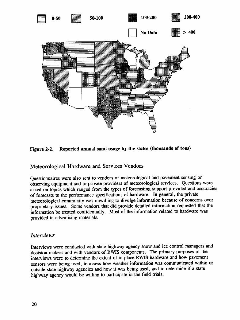
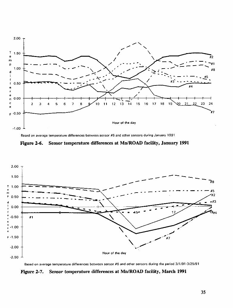
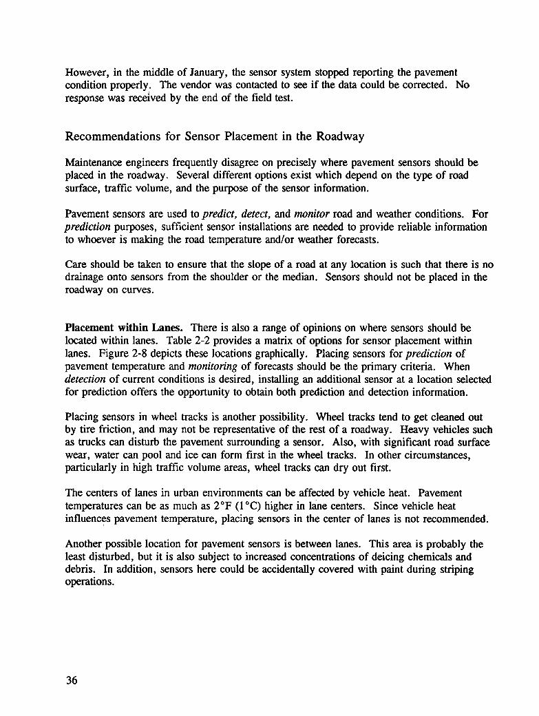
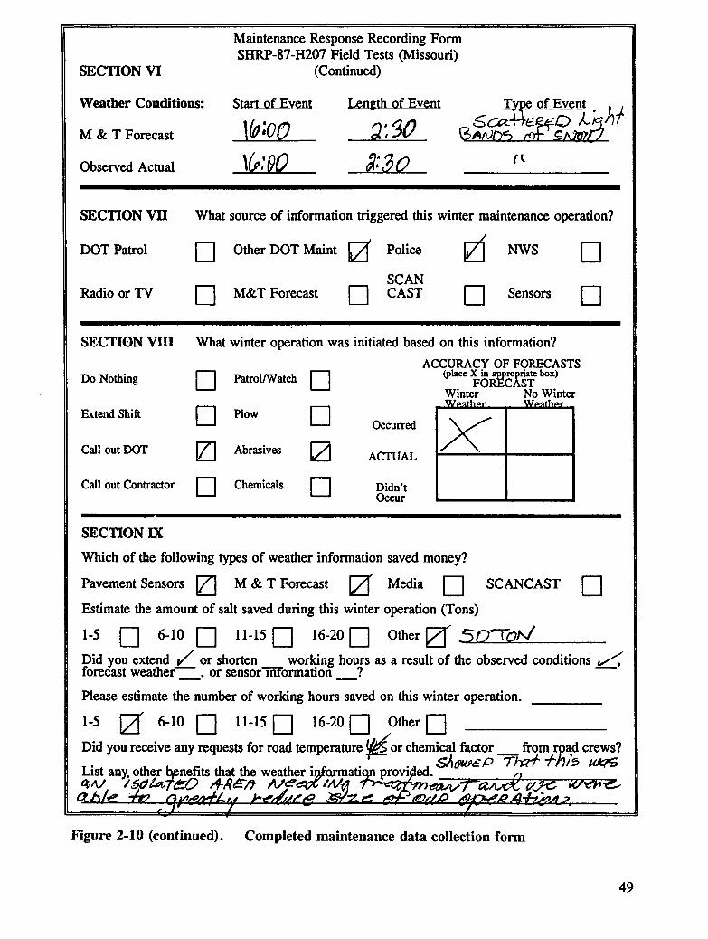
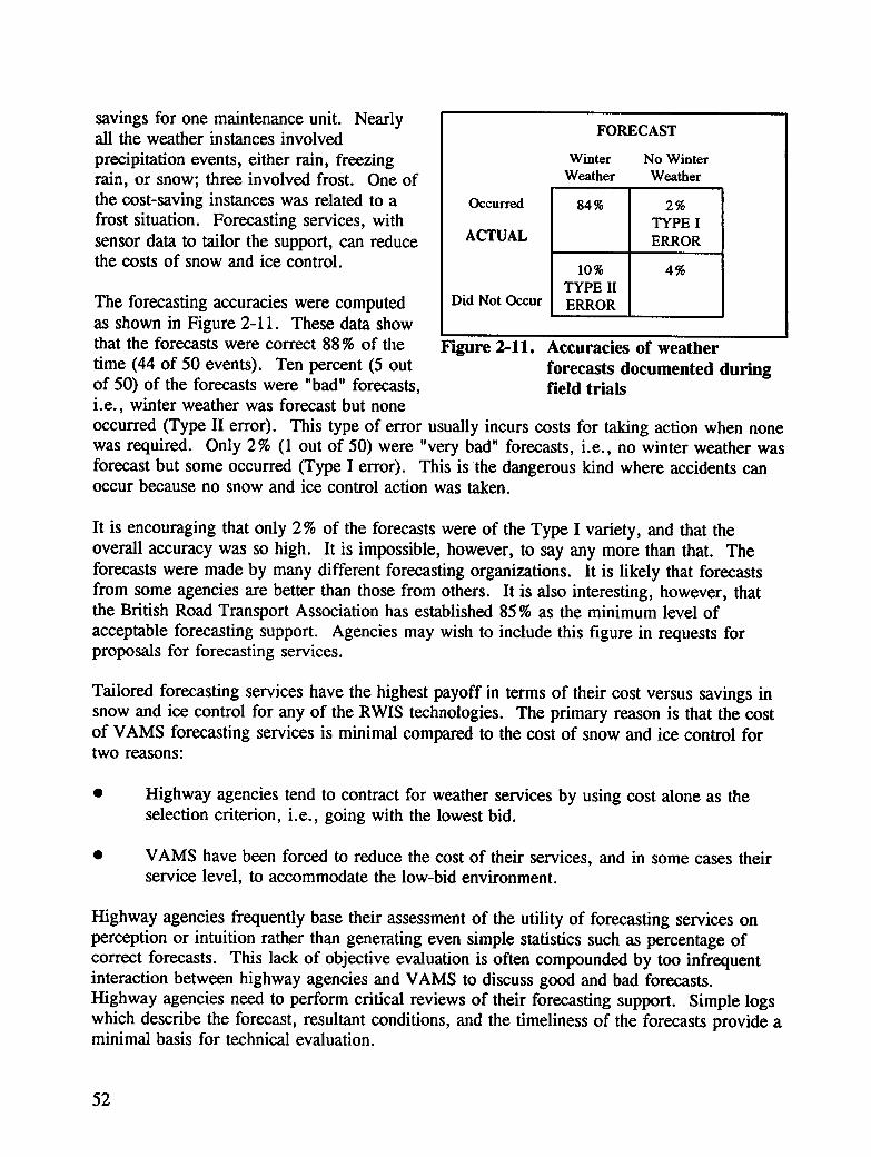
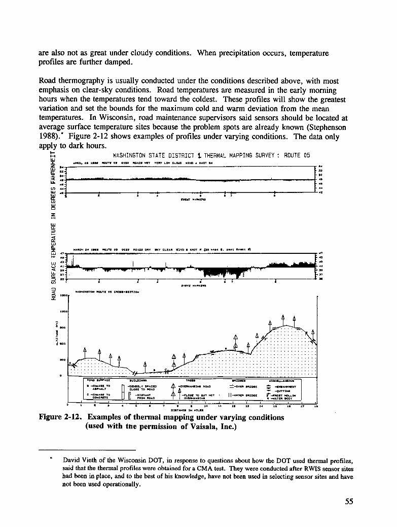
Figure 2-1. Reported annual salt usage by the states (thousands of tons) ........ 19Figure 2-2. Reported annual sand usage by the states (thousands of tons) ........ 20Figure 2-3. Sample maintenance data collection form .................... 24Figure 2-4. Sample pavement temperature data collection form .............. 26Figure 2-5. Sensor locations in the Mn/ROAD pavement .................. 33Figure 2-6. Sensor temperature differences at Mn/ROAD facility, January 1991 . . . 35Figure 2-7. Sensor temperature differences at Mn/ROAD facility, March 1991 .... 35Figure 2-8. Lane orientation ................................... 37Figure 2-9. Sensor placement in a lane ............................. 38Figure 2-10. Completed maintenance data collection form .................. 48Figure 2-11. Accuracies of weather forecasts documented during field trials ....... 52Figure 2-12. Examples of thermal mapping under varying conditions (Used with the
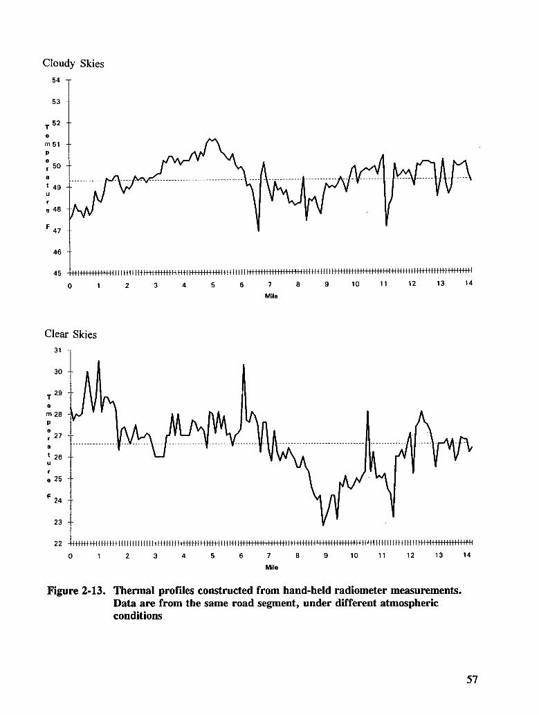
permission of Vaisala, Inc.) ............................ 55Figure 2-13. Thermal profiles constructed from hand-held radiometer measurements.
Data are from the same road segment, under different atmosphericconditions ....................................... 57
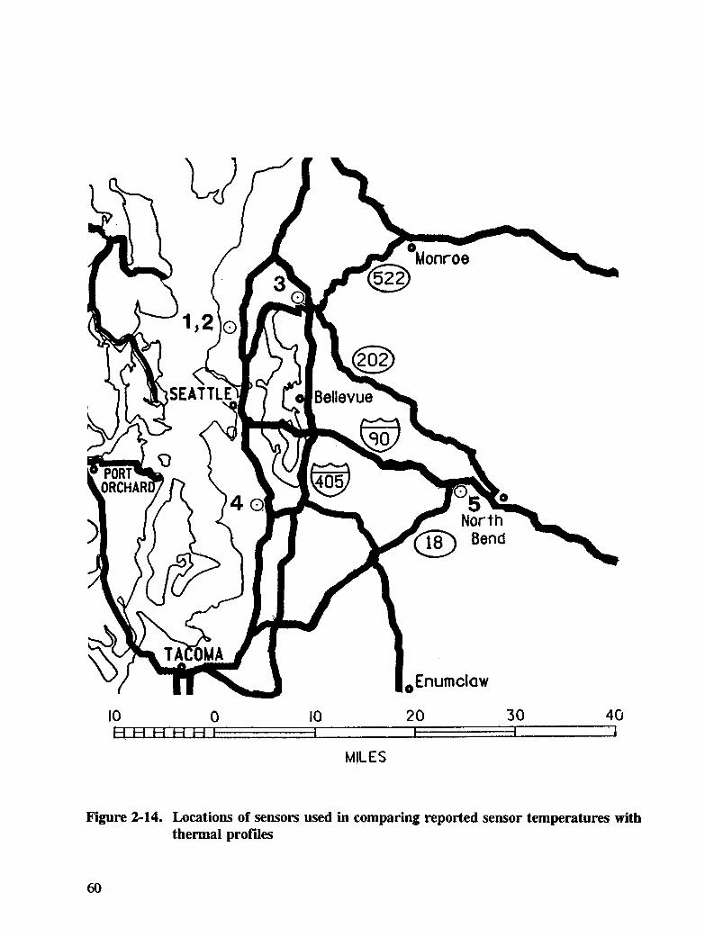
Figure 2-14. Locations of sensors used in comparing reported sensor temperatureswith thermal profiles ................................ 60
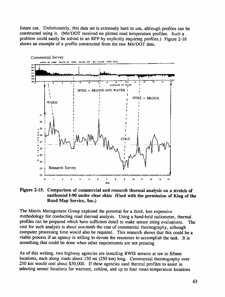
Figure 2-15. Comparison of commercial and research thermal analysis on a stretchof eastbound 1-90 under clear skies (Used with the permission of Kingof the Road Map Service, Inc.) .......................... 63
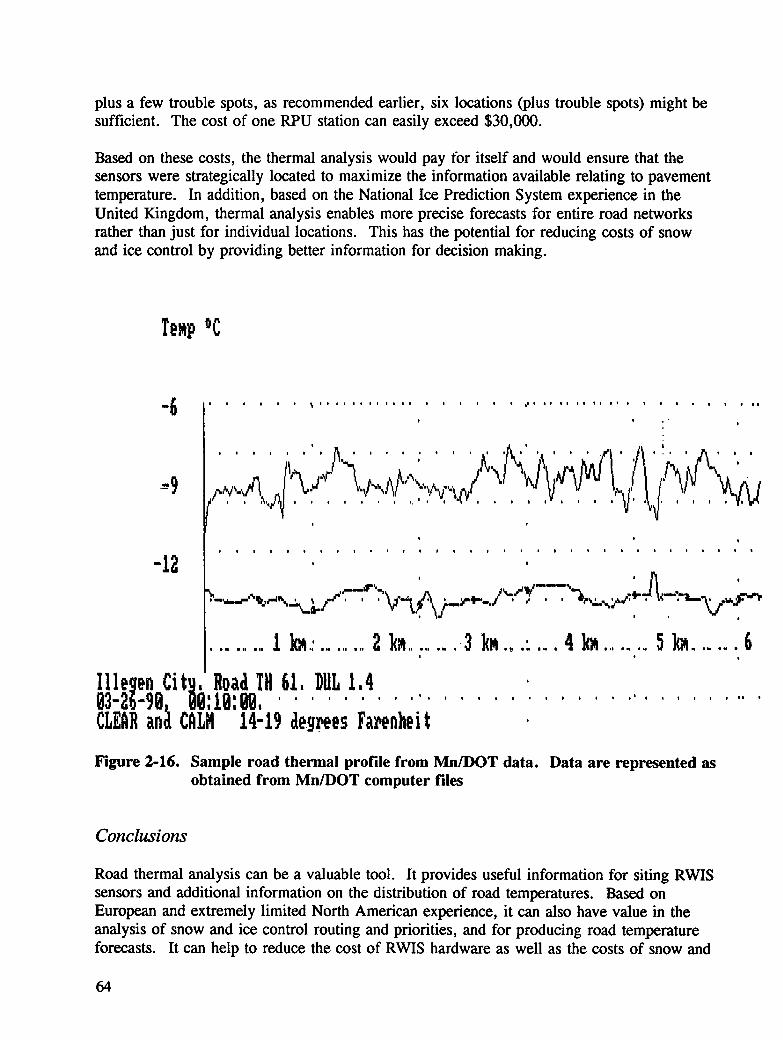
Figure 2-16. Sample road thermal profile from Mn/DOT data. Data are representedas obtained from Mn/DOT computer files ................... 64
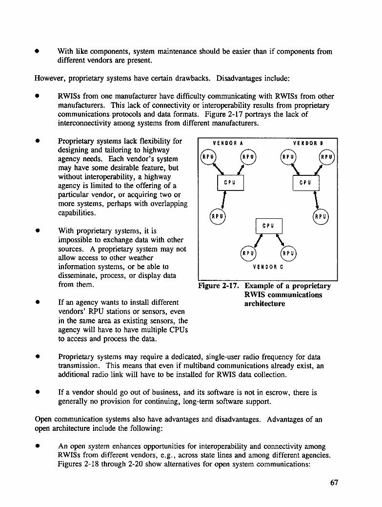
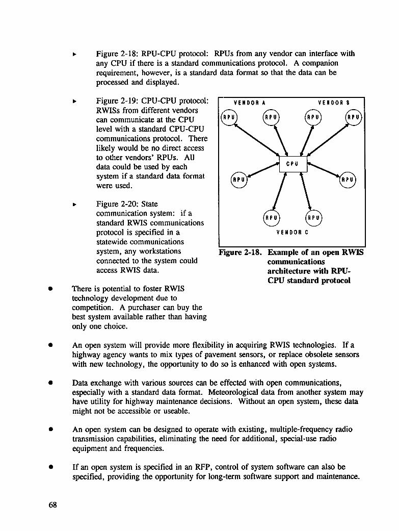
Figure 2-17. Example of a proprietary RWIS communications architecture ....... 67Figure 2-18. Example of an open RWIS communications architecture with RPU-CPU
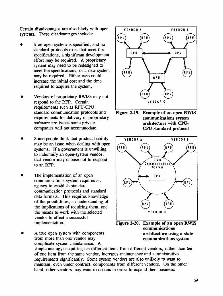
standard protocol .................................. 68Figure 2-19. Example of an open RWIS communications system architecture with
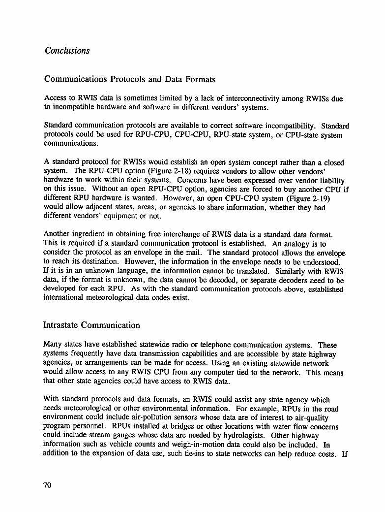
CPU-CPU standard protocol ............................ 69Figure 2-20. Example of an open RWIS communications architecture using a state
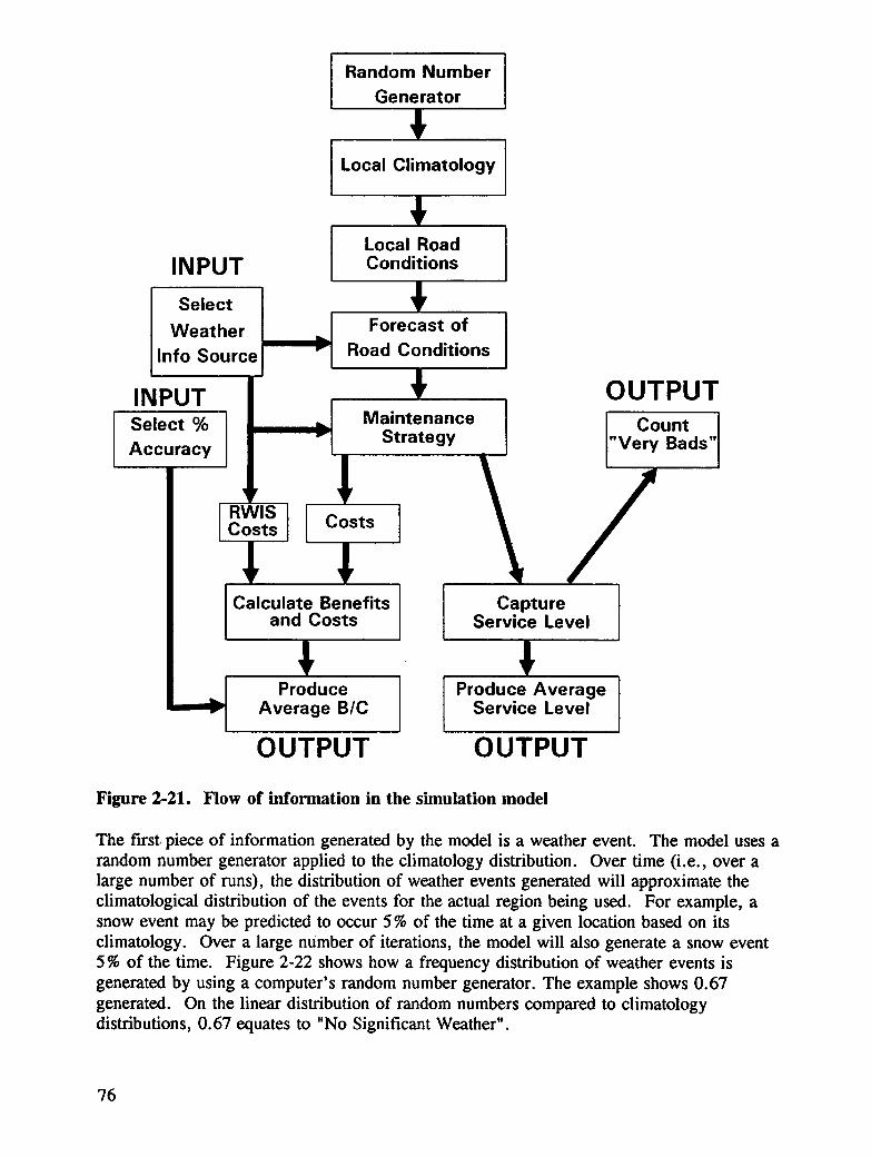
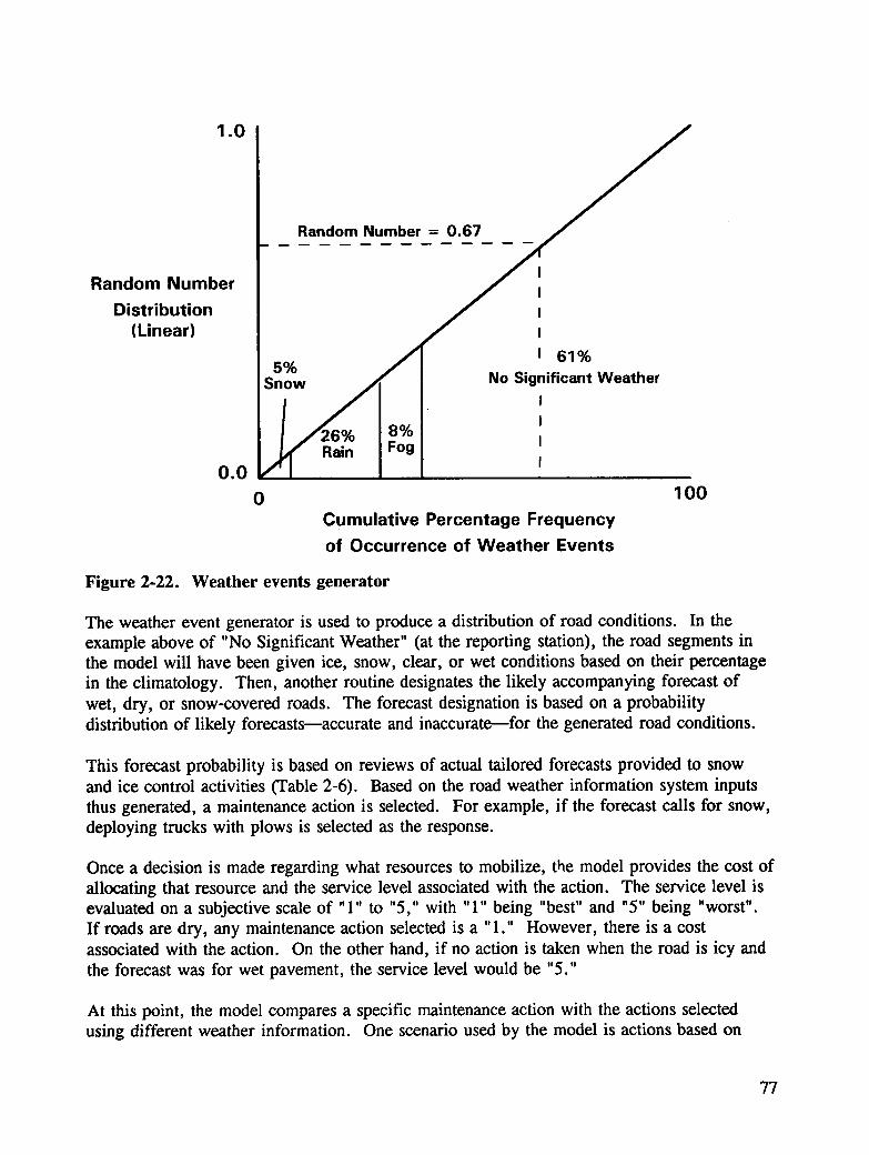
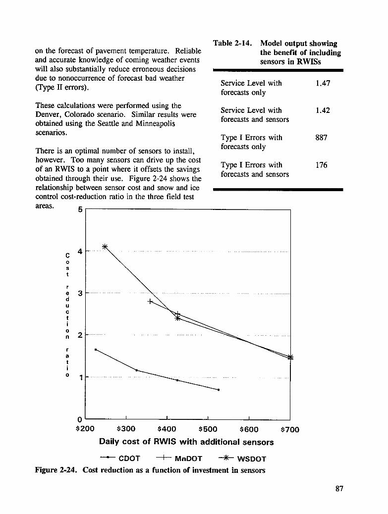
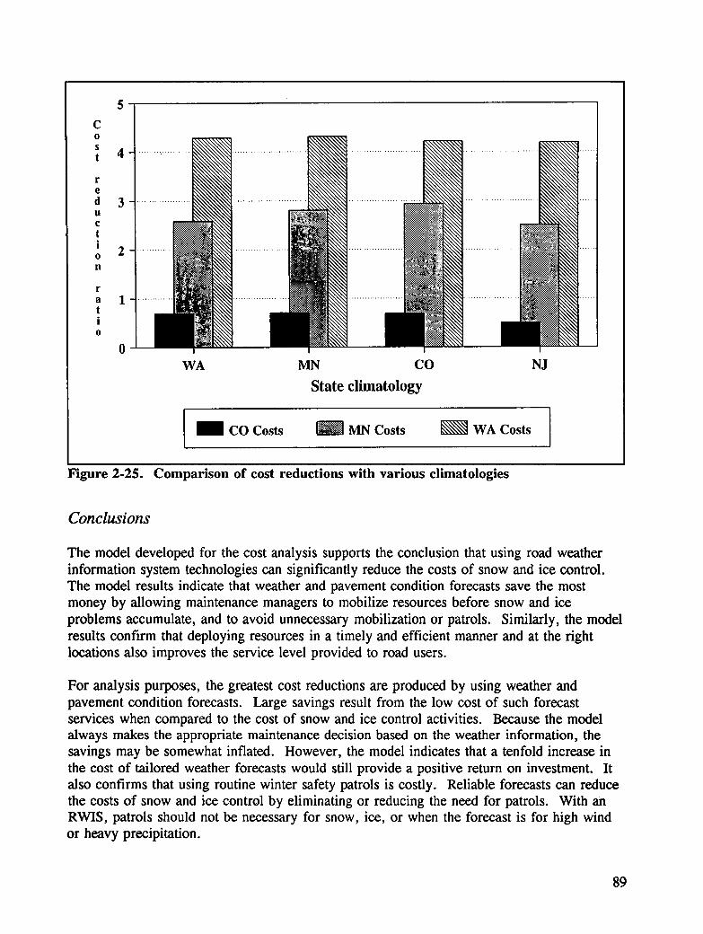
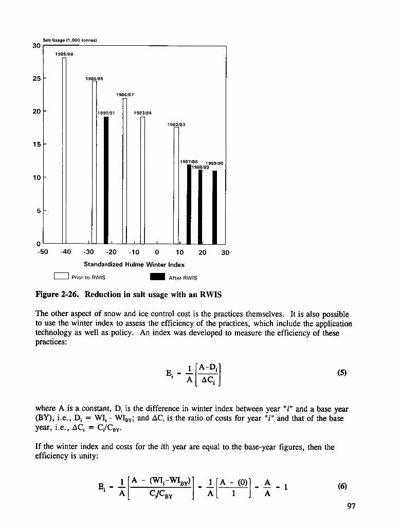
communications system ............................... 69Figure 2-21. Flow of information in the simulation model .................. 76Figure 2-22. Weather events generator ............................. 77Figure 2-23. Forecast decision matrix .............................. 82Figure 2-24. Cost reduction as a function of investment in sensors ............ 87Figure 2-25. Comparison of cost reductions with various climatologies .......... 89Figure 2-26. Reduction in salt usage with an RWlS ...................... 97
ix
List of Tables
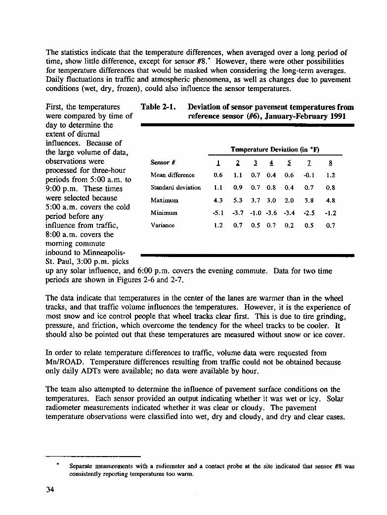
Table 2-1. Deviation of sensor pavement temperatures from reference sensor (#6),January-February 1991 ............................... 34
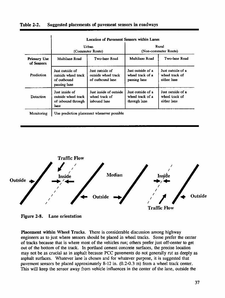
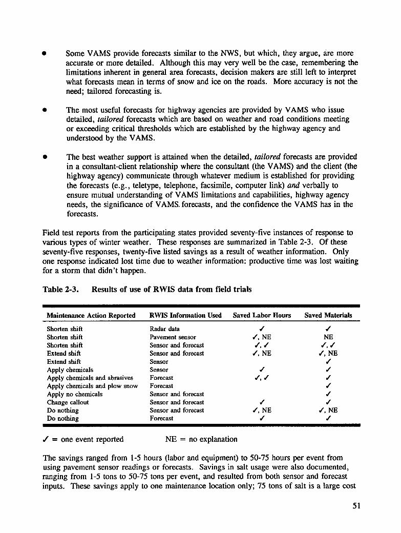
Table 2-2. Suggested placements of pavement sensors in roadways ........... 37Table 2-3. Results of use of RWIS data from field trials ................. 51
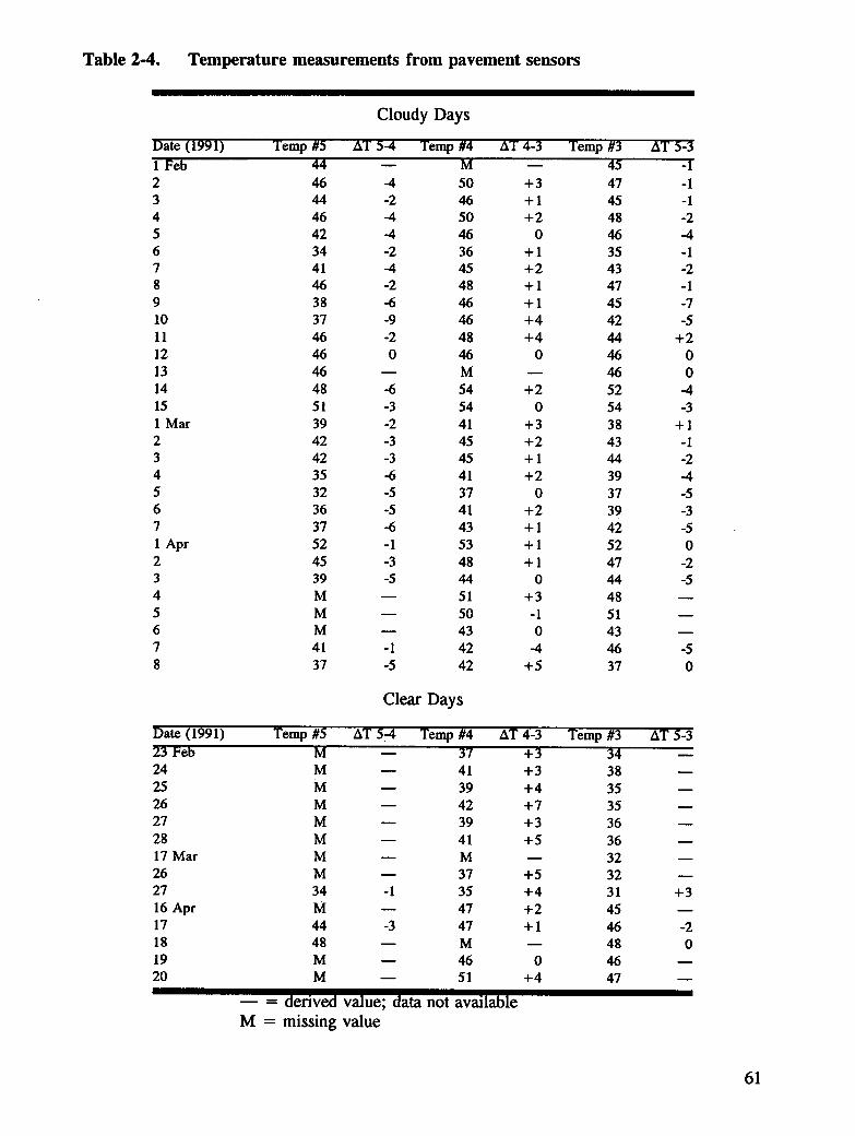
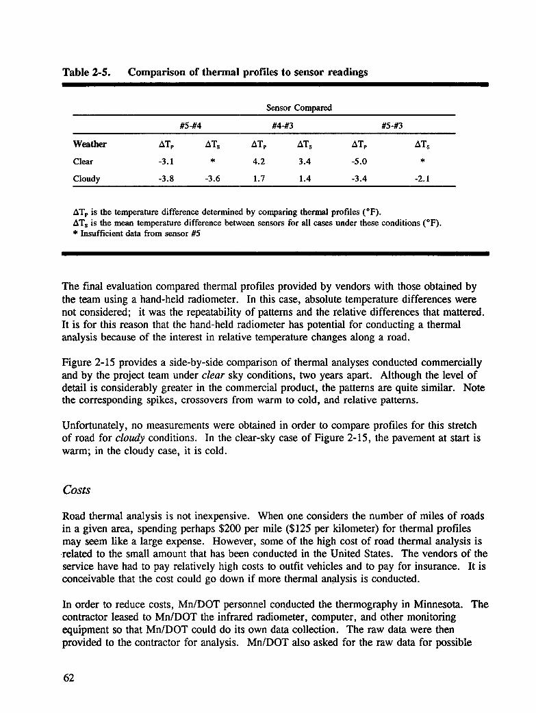
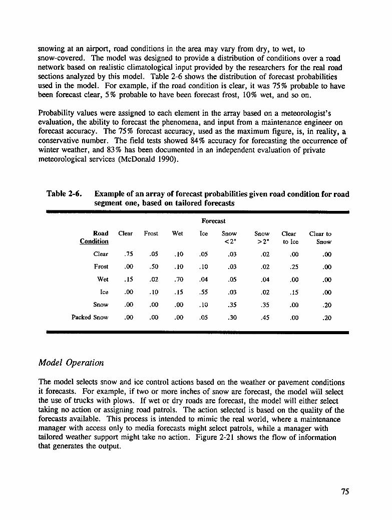
Table 2-4. Temperature measurements from pavement sensors .............. 61Table 2-5. Comparison of thermal profiles to sensor readings .............. 62Table 2-6. Example of an array of forecast probabilities given road condition for
road segment one, based on tailored forecasts ................. 75Table 2-7. Climatology of weather events .......................... 79Table 2-8. Resources matrix .................................. 79
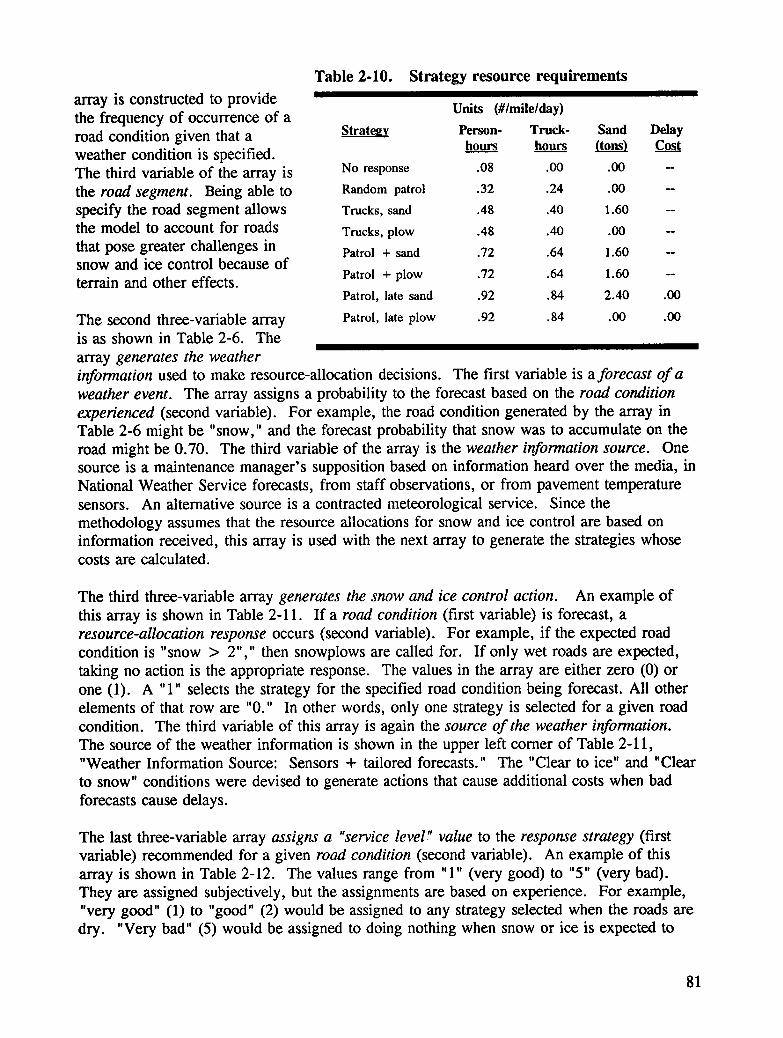
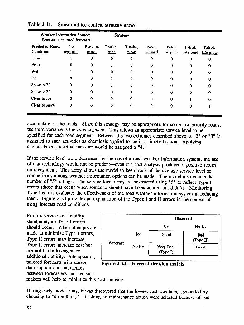
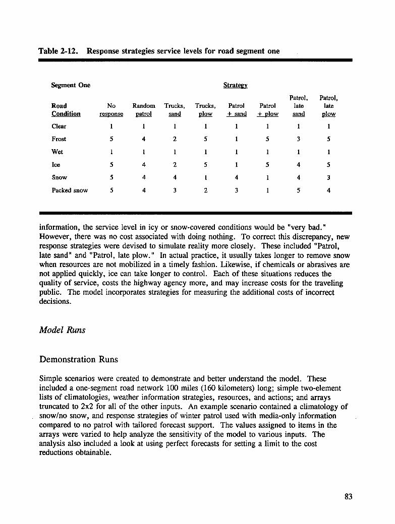
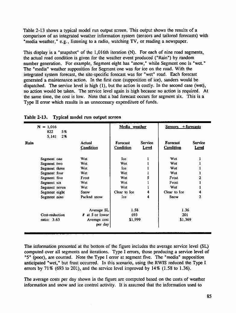
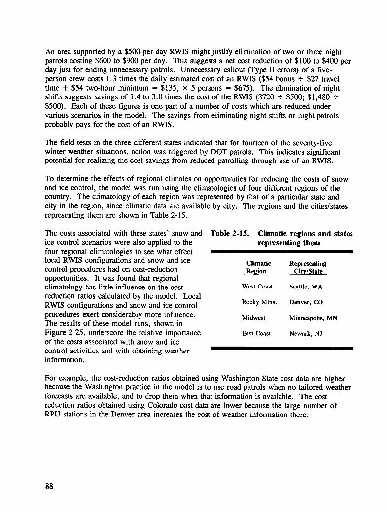
Table 2-9. Daily cost of weather information options ................... 80Table 2-10. Strategy resource requirements .......................... 81Table 2-11. Snow and ice control strategy array ....................... 82Table 2-12. Response strategies service levels for road segment one ........... 83Table 2-13. Typical model run output screen ......................... 85Table 2-14. Model output showing the benefit of including sensors in RWISs ..... 87Table 2-15. Climatic regions and states representing them ................. 88
xi
Abstract
This report provides an overview of roadway snow and ice control practices, the types ofroad weather information currently available, the means for communicating road weatherinformation, and the uses for such information in roadway snow and ice control. The reportpresents the results of field tests conducted to answer questions on the location of roadweather information systems (RWIS), and to discuss a methodology used to determinepossible cost-reduction ranges for RWIS implementation in support of roadway snow and icecontrol. Finally, the report presents conclusions and recommendations for the use of RWISby state and local highway maintenance agencies in support of snow and ice controlactivities.
Executive Summary
In order to better respond to the transportation needs of industry and the travelling public,state highway agencies are seeking new ways to ensure safer driving conditions on majorhighways during all weather conditions. Highway agencies also are looking for ways to uselabor, equipment, and materials as cost-effectively as possible. Weather technologies canhelp snow and ice control managers make more timely and efficient decisions to enable themto reduce costs and improve service. Several countries in Europe have establishednationwide networks of weather data-gathering systems to provide decision information to"roadmasters." These systems are road weather information systems (RWIS).
The range of weather technologies includes meteorological sensors to gather weatherinformation in the highway environment, sensors in the roadway to collect pavementcondition information, thermographic analysis of roads to develop temperature profiles ofroad networks, and forecasts of both weather and pavement conditions.
Under Contract SHRP-87-H-207, Storm Monitoring/Communications, each of thesetechnologies was tested in one or more states. Seven states participated in this study:Massachusetts, New Jersey, Michigan, Minnesota, Missouri, Colorado, and Washington.These states were selected because of their implementation of some of the technology, theiruse of different snow and ice control practices, and their different climates. Information wascollected during the 1990-1991 winter in order to conduct a cost analysis using thesetechnologies for snow and ice control, and to determine what kinds of technologies should beused and where they should be used. In addition, highway agencies in the United States andCanada were surveyed with questionnaires to determine their annual cost for weatherinformation. Highway maintenance managers were interviewed in person. A literaturesearch determined the existing technologies worldwide.
This final report provides details on the conduct of the investigation, describes thedevelopment of a methodology for performing the cost analysis, documents the conclusionsfrom the investigation, and lists recommendations for states and other levels of governmentto consider when implementing RWIS technologies. In addition to this final report, RoadWeather Information Systems. Vol. 2 Implementation Guide has been produced whichsupplements the research results presented in this report and which will assist highwayagencies in implementing RWIS.
This investigation concluded that the use of RWlS can be a cost-effective method to reducecosts and improve roadway snow and ice control.
• The best return on investment occurs when highway maintenance managers usedetailed forecasts of weather events and pavement conditions in their snow and icecontrol decisions. This is true for highway agencies with large or small snow and iceproblems.
• An RWIS that blends data inputs from sensors and thermal evidence into detailedforecasts tailored to the needs of snow and ice control managers offers the opportunityfor a significant return on investment close to 500%, and significantly improves theservice level on the roads, and greatly decreases the frequency of decision errors.
• RWIS sensors provide a generally reliable means to monitor, detect, and assistin the prediction of road temperatures and weather and pavement conditions.Sensor data, when made available to forecasters, allow for much betterforecasts of road temperatures and icing. Hence, they allow for an improvedsnow and ice control service level and reduced decision errors.
• Because of heat transfer differences among sensors, pavement, road subgrade,and solar energy, pavement sensor temperatures may differ by several degreesfrom pavement temperature readings under clear sky conditions.
• Sensor reliability and accurate output require a preventive or routinemaintenance program, and at least annual calibration of sensors.
• Road thermal analysis, when combined with sensor data, can be a cost-effective anduseful tool for improving pavement temperature and condition forecasts. Roadthermal analysis can assist in determining locations for RWIS sensors, reduce thenumber of locations required, and thereby reduce hardware costs.
• In order for RWIS data to be integrated properly into snow and ice control decisionprocesses, effective communications must be established to ensure the timely flow ofinformation.
• Sensor data, weather information, and pavement temperature predictions needto get to snow and ice control decision makers. In order to accomplish this ina timely manner, portable computers with modems should be made available tothe lowest level of decision makers in the majority of cases.
• Sensor data need to be available to the agency/firm providing the forecastservices. This availability should include on-line and dial-up access.
• Effective communications must be established between forecasters and
maintenance managers to ensure that forecasters understand the needs of themanagers, that the managers understand the weather information, and that theforecasters know how well the information satisfies the managers' needs.
• Data dissemination practices designed to hold down communication costs, such astransmitting information only when certain parameter thresholds are crossed, limit the
4
use of RWIS data. Data gaps on the order of days have occurred. These gapspreclude post-event analysis, applied research using the data, and the development offorecast techniques. Such practices should be modified to avoid these limitations andincrease the value of RWlS data.
• Philosophical and psychological barriers exist to integrating RWlS technologies intosnow and ice control operations. Individual barriers include distrust of weatherforecasts, fear of change, and the perception that technology is difficult to implement.These barriers can be overcome through behavioral changes resulting from training.Organizational barriers include problems with management and labor, perceivingRWlS implementation as a top-down-directed initiative, and having little or noparticipation and support at the implementation level. These barriers requireorganizational behavior change and also can be overcome with training plusmanagement initiatives.
• Problems exist in contracting for weather forecasting services and acquiring RWIShardware.
• Highway agencies frequently contract for weather services using low-bidprocedures, resulting in services that inadequately meet the agencies' needs.
• Many highway agencies interested in pursuing acquisitions write requests forproposals (RFPs) which parrot vendor specifications whether appropriate ornot.
Agencies considering investment in an RWIS should consider the followingrecommendations:
• All highway agencies that perform snow and ice control should assess the benefit ofcontracting with a value-added meteorological service (VAMS) for weather and roadcondition forecasting.
• Highway agencies should contract for meteorological services using an RFP,consultant selection, negotiated-price procedure. Highway agencies should usetechnical evaluation criteria for selection and not just cost. Some highway agenciesmight consider developing meteorological expertise on their staffs.
• Each highway agency that has either an RWIS in use, or desires to develop one,should obtain weather support from a designated weather advisor who works directlywith snow and ice control personnel to assist in the acquisition and implementation ofRWIS technologies, to provide guidance on sensor acquisition and siting, to helpcontract for weather services, and to provide staff training on the use of the RWlS forsnow and ice control. The weather advisor should be knowledgeable concerningmeteorology and RWIS technologies. He/she can be a part-time, shared, or full-timeexisting employee, new hire, consultant, or VAMS.
5
• Highway agencies planning to acquire RWIS sensors should consider using roadthermal analysis and road crew knowledge to assist with sensor siting and forecastingof road conditions.
• Any highway agency acquiring RWIS technologies should develop a training programto assist the integration of RWIS information into snow and ice control decisionprocesses and the development of management strategies.
• All highway agencies should require that RWIS data be acquired from sensors at leastonce each hour. If no data are received for over an hour, action should be taken tocorrect any problems.
• Data from an RWIS should be archived. Data can be of great value for research,performing local forecast studies, and for records of road and weather conditions andmaintenance actions for liability purposes.
• All highway agencies with RWlS hardware should implement a routine maintenanceprogram. Sensors should be calibrated annually. A standard calibration procedureshould be adopted.
• Involve the parties affected by change in the process of change. Tap the knowledgeof road crews about the roads they maintain, for example. The benefits of such anapproach are many: it recognizes the value of the people within the organization;opinions about the new system can be discussed at stages where protocol and designchanges still can be made; people involved in change are more likely to understandand actually use the system; and longstanding issues regarding the snow and icecontrol practices of a highway agency can be addressed. Much as RWlS forecastsmust be tailored to an agency, its actual system must also fit the agency.
6
1
Introduction
Statement of the Problem
Controlling snow and ice on roadways requires large expenditures for labor, equipment, andmaterials. The United States and the provinces of Canada spend over $2 billion annually onsnow and ice control. Snow and ice control costs could be reduced by improving the abilityof highway agencies to select an appropriate strategy and carry it out in the most timelyfashion.
The inability to accurately predict storm conditions and pavement conditions, and tocommunicate rapidly changing conditions to snow-removal forces and the travelling public,result in excessive and unnecessary expenditures. Calling crews out for prestorm treatmentwhen a storm doesn't materialize is a waste of resources. Delaying treatment to be certain astorm is of sufficient magnitude to warrant attention eliminates the advantages of earlytreatment and increases the amount of resources necessary to return the road system to anormal condition. An efficient snow and ice control process would provide for themobilization of just the right amount of personnel and equipment at just the right time.
An emerging technology which uses weather and roadway sensors to provide currentinformation to snow and ice managers could provide timely notice of changing temperature,of snow or freezing rain beginning to fall, or of the amount of chemical remaining on thepavement. At the time this project was initiated, over ten states had installed pavementsensors for snow and ice control, but little information regarding performance or cost-effectiveness was available.
If the information produced by sensors is not integrated into a forecast system and is not usedto generate accurate predictions of weather and pavement conditions, sensors have onlylimited usefulness, and their full potential is not realized. Fragmentary information is notsufficient for proper crew scheduling.
Effective storm management requires the capability to predict the need for snow and icecontrol four to twelve hours in advance. This capability would enable supervisors to send
7
workers home to rest before a storm hits and to estimate how many workers will be neededand when they should return. It would also enable supervisors to plan routine maintenancework to keep employees as productive as possible when freezing temperatures or snowfall arenot forecast.
Rapid communication, both on a regional basis and within the structure of individualjurisdictions, is also necessary for effective coordination of snow-removal efforts.
The precursors to road weather information systems (RWIS) were initially installed atairports in this country. Their information was used to assist airport authorities in theirconduct of snow and ice control. Atmospheric and pavement sensors were installed atairfields, usually near the ends of runways, runway intersections, and on parking ramps.These sensors sent their data to processors in airfield operations offices where supervisorsmade decisions concerning chemical applications for deicing and snow plowing.
The snow and ice control problems of highway authorities only differ in magnitude andmethods for treatment. Similar systems were sold to highway agencies and other agencies.Remote processing units (RPU) with atmospheric and pavement sensors were installed alonghighways, and central processing units (CPU) were installed in highway maintenancefacilities. These systems were generally installed on a research or test basis. In simplisticterms, when more RWISs were desired, additional RPUs and a CPU were installed inanother maintenance area of responsibility.
Road weather information systems are made up of pavement sensors and other componentssimilar to those in standard weather information systems. An RWIS may contain:
• Meteorological sensors which measure atmospheric temperature, relativehumidity or dew point," wind speed and direction, and precipitation;
• Pavement sensors which measure surface temperature, subgrade temperature,surface condition (wet, dry, or frozen), the amount of deicing chemical on thepavement, or the freezing point of a wet surface;
• Temperature profiles of roadways based on road thermal analysis;
• Site-specific forecasts of weather and pavement conditions tailored to ahighway agency's needs;
• Other weather information for use by meteorologists and snow and ice controlmanagers, such as radar images and National Weather Service forecasts;
• Communications and data processing and display capabilities for datadissemination and presentation; and
* Dew point is the temperature at which the atmosphere would be saturated (100% relative humidity) ifcooled. It is used in the calculation of relative humidity.
8
• Weather support to agency staff that allows for close coordination andconsultation between meteorologist and decision maker.
• A plan for an agency to use its RWIS data to create and maintain a preventiveactivity program for winter weather problems.
Each component of an RWIS is specialized because of its application. It is important tounderstand their differences and applications. To establish a common basis of understanding,the following sections describe standard and road weather information system components.
Standard Weather Information
There are different types of weather information available to different groups. The generalpublic gets area weather information provided by the National Weather Service, broadcastand print media, and in some cases, specialized television broadcasts such as The WeatherChannel, AM Weather on the Public Broadcasting Service, or cable television broadcasts ofNational Weather Service forecasts and weather radar. Finally, National Oceanic andAtmospheric Administration Weather Radio provides continuous broadcasts of weatherobservations, forecasts, and in some instances, specialized information such as roadconditions. For the most part, all of this weather information is for large areas and definesaverage conditions or a range of conditions, but not conditions for specific locations.
There are two types of weather information: observations and forecasts.
Observations
Weather observations provide information on the current state of the atmosphere. Theseobservations are usually provided hourly, or more often if significant changes occur. Typicalobservations describe sky cover (cloudy, partly cloudy, clear), the type of weather occurring(rain, snow), air temperature, relative humidity, and wind direction and speed. Frequently,the atmospheric (barometric) pressure and the pressure tendency (rising, falling, or steady) isgiven. Aviation observations contain additional information. Sky cover information is moredetailed and includes the heights and amounts of clouds, the visibility distance, and anyrestrictions to visibility (fog, smoke, dust, snow). Aviation observations also include the
dew point, a pressure reading for pilots to use for setting altimeters, and runway information.
Weather observations are also used by the meteorology community to generate forecasts.For instance, a forecast for conditions one hour from now could very well be the latestobservation. Observations are monitored to check the accuracy of earlier forecasts. Ifobserved weather conditions begin to deviate significantly from forecast conditions, then theforecasts may require change.
A weather observation usually contains information obtained from sensors such asthermometers for temperature and anemometers for wind direction and speed. Additional
9
observations are provided by instruments borne aloft by balloons in order to obtain upperatmospheric temperature, humidity, and wind data; by weather radars that detect or monitorprecipitation and severe weather; and by satellites. Data from these observations are mostlyused to provide initial or boundary conditions for meteorological computer models, to assistin severe weather forecasting, and to support aviation.
Additional information must be gathered by human observers of the sky and weatherconditions. Humans also have to record the instrument observations and encode observationsfor dissemination. Both the National Weather Service and the Federal Aviation
Administration are in the process of installing automated observing systems around thecountry. Considerable research has gone into the development of systems to provideinformation to the aviation and meteorological communities without human interaction.
Forecasts
Weather forecasts describe expected future weather conditions in general terms for an area.For example, forecasts may be issued for urban areas, coastal areas, or mountains. Mostpublic forecasts are issued by the National Weather Service and are frequently retransmittedby broadcast media. Some media either have their own meteorological staffs which producetheir own forecasts, or they contract for weather services from value-added meteorologicalservices (VAMS). Public forecasts rarely provide detailed information which can be relatedto specific locations. In most cases, users must interpret these forecasts to determine thepotential impact of the expected weather.
Aviation weather forecasts, on the other hand, are usually site-specific or deal with aparticular route of flight. Detailed forecasts are issued by the National Weather Service forlarger airports, and in some cases, general aviation airfields. These forecasts containprojections of the same conditions contained in aviation observations, i.e., conditions ofimportance to aviators who need to know whether they will be able to take off or land atparticular locations.
Site-specific forecasts usually require the services of VAMS. VAMS use National WeatherService data and forecasts, specialized observations, objective forecast techniques, andmeteorological models to prepare forecasts. VAMS customers frequently have specialneeds----critical thresholds for decisions. VAMS tailor their forecasts to meet a user's needs.
Road Weather Information
The primary reason for using forecast information is to help make decisions whether toundertake certain activities in a timely manner. Without forecast information, decisionsregarding activities must be based on the actual occurrence of weather phenomena, andtherefore cannot be made much in advance of the activities.
10
So it is with snow and ice control on our highways. A supervisor can make resourceallocation decisions based on forecasts of weather and pavement conditions (plan ahead, moreeconomical), or rely on observations of those road conditions (react, more costly).
Observations
Road weather observations are similar to standard weather observations in many ways. Theyprovide information about weather conditions in the road environment and the conditions of
the pavement. This information is usually gathered by meteorological or pavement sensors.
Meteorological instruments located along roadways gather data on temperature, dew point,wind speed and direction, and the occurrence of precipitation. Sensors placed in the
l pavement monitor the pavement temperature; determine whether the pavement is dry, wet, or
I ice-covered; measure the relative concentration of any deicing chemicals on the road surface;and calculate the temperature at which the moisture on a surface would freeze. Atemperature probe is also sometimes placed about 20 in. (0.5 m) below the surface. The
subsurface temperature is used with other data to determine if heat is flowing to or awayfrom the surface.
These observed parameters are important to understanding what is taking place on the road.For instance, road temperature and precipitation data are key to whether ice or snow canbond to the pavement, or whether ice can exist. Road temperature and dew point are key towhether frost can form on the surface. These data are also important for the development offorecasts of these conditions. It is the forecasts of these weather events that are the key tosuccessful decision making, improved efficiency, and reduced costs of snow and ice control.
Forecasts
Forecasts can and should be obtained for both weather and road conditions.
Forecasts of pavement temperature have been made possible with the development ofcomputer models that use observations of conditions in the road to produce surfacetemperature forecasts accurately out twenty-four hours in the future. This lead time allowsmanagers to plan allocation of resources during the day for the following night andsucceeding morning. Knowledge that the pavement temperature will or will not go belowfreezing can be critical factor in a snow and ice control decision.
Better decisions can be made with forecasts tailored to a decision maker's needs. Snow and
ice control managers need tO know not only that a weather event such as snow is expected,but also how much, where, when, and for how long. Managers use some critical thresholdsto make resource allocation decisions, such as > 2 in. (5 cm) of snow for mounting plows,> 6 in. (15 cm) for calling out contractors, or storm duration greater than twelve hours for
emergency shift scheduling.
11
Much of the information important to snow and ice control supervisors is not available fromstandard sources of information. If detailed forecasts of weather and road conditions are tobe obtained, it is advisable for an agency to acquire a value-added meteorological service(VAMS). A VAMS could be a state agency, a state-funded weather service as is found inavalanche forecasting, or a private meteorological service.
VAMS provide a wide range of forecasting services, including short-range (0-4 hours), mid-range (4-24 hours), and long-range (24 hours or more) forecasts of weather events. Eachrange has utility in making decisions for snow and ice control. In addition to weather eventforecasts, road condition forecasts are necessary. These conditions include snow cover,icing, and frost. Road condition forecasts require pavement temperature forecasts. Roadtemperature forecasts are somewhat more reliable than atmospheric temperature forecasts.The thermal energy balance at the pavement surface is easier to model than the atmosphere.More predictable temperatures are possible there than for the atmosphere.
Road Thermal Analysis
One form of road thermal analysis, road thermography, was developed simultaneously in theUnited Kingdom by Dr. John Thornes of The University of Birmingham, and in Sweden byProfessor Sven Lindqvist of The University of Gothenburg (Thornes 1972, Lindqvist 1976).The principle underlying road thermal analysis is that if a temperature is known at a specificlocation, then pavement temperatures can be estimated between sensors. It uses vehicleswith downward-pointing infrared radiometers to collect road surface temperatures every fewmeters. Data are gathered in the early morning hours when surface temperatures tend to bethe coolest and solar heating effects are absent. Data are gathered under clear sky, cloudysky, and wet pavement conditions because the temperature patterns of a road surface differsignificantly under each of these conditions. The raw data are used to prepare temperatureprofiles along a road. Under the same sky and wind conditions, the temperature profiles fora road will have the same shape over time. These profiles supplement sensor data since asensor only provides pavement temperatures at one location.
Supplemental data are usually also annotated to the profiles to indicate areas where theroadway might be shaded from the sun, or where temperatures may be influenced by suchthings as buildings, forests, or bridges. An extension to road thermal analysis is used inSweden to show moisture sources, locations where cold air tends to pool at night, and areas
prone to wind and drifting snow. This extension is called road climatology, and it isdesigned to be used in conjunction with temperature profiles to provide an expanded basis forshort-term forecasting of pavement temperatures and road conditions.
Road thermal analysis has been used to help determine optimal locations for RWIS sensors,to develop alternative plowing and spreading routes for snow and ice control, and to prepareforecasts of road temperatures.
12
Communications
Three paths of communications are required for successful utilization of an RWlS:communication from sensor systems to roadway maintenance centers, communicationbetween snow and ice control managers and private weather services, and communicationfrom highway agencies to the traveling public.
Data Transfer from Sensors
In order for RWIS sensor data to have value, the data must be available to highway agenciesand VAMS. A typical RWIS sensor system includes onsite sensors, a microprocessor tocollect and format the data in digital form, and a transmitter to send the data to users. Themicroprocessor/transmitter is called a remote processing unit (RPU) or outstation. RPUstypically communicate with a central processing unit (CPU) or instation, a computer locatedwhere data from more than one RPU may be gathered.*
An RPU usually transmits data via radio signal or land line. Radio transmissions requireline-of-sight between an RPU and an antenna. In order to get a signal to a CPU, repeaterantennas may be required. State-owned microwave systems provide one of the besttransmission capabilities. Land lines can be dedicated leased telephone lines or state-ownedcables. Data can also be transmitted by cellular telephone in some areas, and these areas areexpanding, although the transmission costs may be high.
Once data are sent to a CPU, they can be retrieved by other computers. Supervisors andmanagers can have real-time access to observations around the clock through the use ofportable computers with telephone modem capability. A supervisor can dial into a CPUfrom any telephone, including at home or while on the road, to monitor data, analyze trends,and acquire the latest forecasts.
Similar capability should also be available to VAMS providing support to highway agencies.Access to observations is key to successful forecasting, and to building a knowledge base ofweather conditions in locations of interest.
Information Transfer between VAMS and Highway Agency
A communications link must also exist between a provider of weather support, the VAMS,and the user of the weather information, the highway agency. There are a number of waysfor the VAMS to transmit and the highway agency to receive weather and pavementcondition forecasts. These include teletype, telephone, facsimile (fax), computer-to-computer, or combinations thereof.
" For greater detail on communications, refer to the Road Weather Information Systems. Vol. 2Implementation Guide prepared under this contract, and to a Transportation Research Board report entitledTransportation Telecommunications (National Research Council, Transportation Research Board 1990).
13
The format of the forecasts can also vary from detailed word descriptions to forms withboxes checked in menu fashion. The information contained in word discussions can be
tailored to the needs of a highway agency, while menu-type forecasts tend to include standardtypes of information provided to all customers. The latter may also require furtherinterpretation by snow and ice control managers, while the former might provide informationin a form ready for decision making.
Another aspect of VAMS-highway agency communication is human interaction. Foreffective communication to take place, a snow and ice control manager must be able to talkwith a meteorologist, and vice versa. For effective communication, the manager mustunderstand what the meteorologist means, and the meteorologist must know what themanager needs. The meteorologist and manager also need to understand each other'scapabilities and limitations. This verbal capability is also necessary for evaluative processesso that the VAMS meteorologists can improve their forecasting, and equally important, getnotified that their forecasts were correct.
Information Dissemination to the Traveling Public
The primary purpose of snow and ice control activities is to maintain roadways that allowreasonably safe travel for the public. However, before travellers venture forth on the roads,they also need to be prepared for whatever the road conditions might be. Travellers, too,need to make decisions based on road condition reports.
Current road conditions are frequently available. Highway agencies apprise the public ofthese by one or more of the following:
• Local television and radio broadcasts
• Highway advisory radio broadcasts
• "800" or "900" highway agency-sponsored phone numbers
• Rest-area broadcasts
• Commercial local-area advisory broadcasts
• NOAA Weather Radio in some areas
• American Automobile Association (AAA) via telephone
• Variable-message signs controlled by transportation centers
_4
• Variable-message signs remotely controlled by sensors, e.g., visibility (fog),precipitation (ice or snow), and wind.
This list is not intended to be all-inclusive. It does point out that there are many ways forthe public to obtain information, none of which is ideal at all times. It also shows that thepotential exists for different information being provided simultaneously. This can lead tomistrust or eventual disuse. However, because of interest, curiosity, or real needs forweather information in routing or timing trips, the public is likely to demand pertinentobservations and forecasts when RWISs are more widely established.
15
2
Conduct of the Research
In order to achieve the stated project objectives of identifying promising RWIS technologiesand evaluating their cost-effectiveness, research was undertaken in a number of functionalareas. These included pavement and meteorological sensors, road meteorology sources(especially tailored, site-specific forecasts), road thermal analysis, RWIS communicationsarchitectures, a computerized cost analysis, and development of an index for specifyingwinter severity. These investigations revealed a great deal about the ability of RWlStechnologies to improve the effectiveness and reduce the costs of highway snow and icecontrol activities.
The Investigations
The project focused early on information gathering to determine the state of the art inmeasuring road surface conditions and meteorological conditions in the road environment, todetermine the extent of use of road weather information systems within and outside thiscountry, and to ascertain the potential for use of road weather information in support of snowand ice control activities in the United States. Information was gathered from an in-depthsearch of global literature on the subject of monitoring weather and road conditions, throughwritten questionnaire surveys, through in-person interviews with snow and ice controlmanagers, and through field tests of RWlS technologies.
Literature Search
As soon as this project was initiated, an extensive literature search was undertaken to assist
in the determination of the state of the art in RWIS development and use. A large body ofknowledge was found to exist in Europe. Two large efforts there were focusing considerableattention on RWIS development and testing.
First, through the European Community's (EUCO) Cooperation in the Field of Scientific andTechnical Research (COST) program, member countries first performed an analysis of
17
potential RWlS use to help with snow and ice control. The results were extremelyencouraging (EUCO-COST 30 1983), and a project, COST 309, was initiated for sharinginformation and technology, testing RWIS hardware, and fostering RWlS technologydevelopment. Second, under the auspices of the Permanent International Assembly of RoadCongresses (PIARC), which meets every four years, a Standing European Road WeatherCommission (SERWEC) was formed to enhance the exchange of information and technologywithin the research community. In 1990, SERWEC was changed to the StandingInternational Road Weather Commission (SIRWEC) to reflect the inclusion of representativesfrom countries outside Europe, including the United States.
An extensive bibliography of RWIS-related literature is included with this report.Information from SIRWEC is either published by the individual researchers or appears in theSIRWEC newsletter, Highway Meteorology.
It is important to note that for a variety of reasons, very little research into RWIS use ordevelopment has been published in the United States. Firstly, the only research conducted inthis country was by state highway agencies. Some of this research is published (e.g., NewJersey Department of Transportation 1988, Minnesota Department of Transportation 1989,Michigan Department of Transportation 1988), but frequently it is used only for internaldecision making. Secondly, until 1990, there was for all practical purposes only one vendorof RWlS hardware in this country. Much of this vendor's technology is proprietary, whereasin Europe, such technology development is often government subsidized and implemented.Thirdly, most of the meteorological support provided to state highway agencies in the UnitedStates comes from value-added meteorological services (VAMS), private companies thatprovide tailored weather support beyond that which the National Weather Service provides.These VAMS tend to be very operationally oriented, and they conduct studies for their ownpurposes. They tend not to publish their findings.
Questionnaires
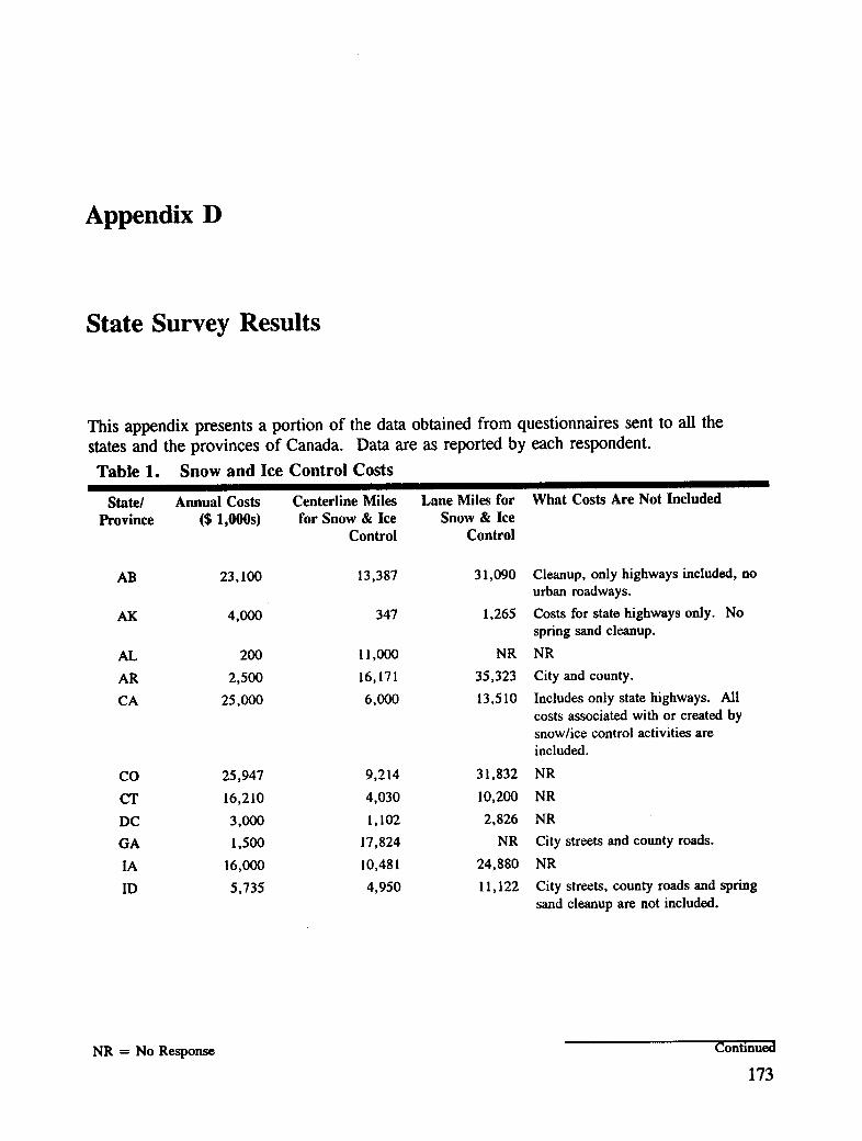
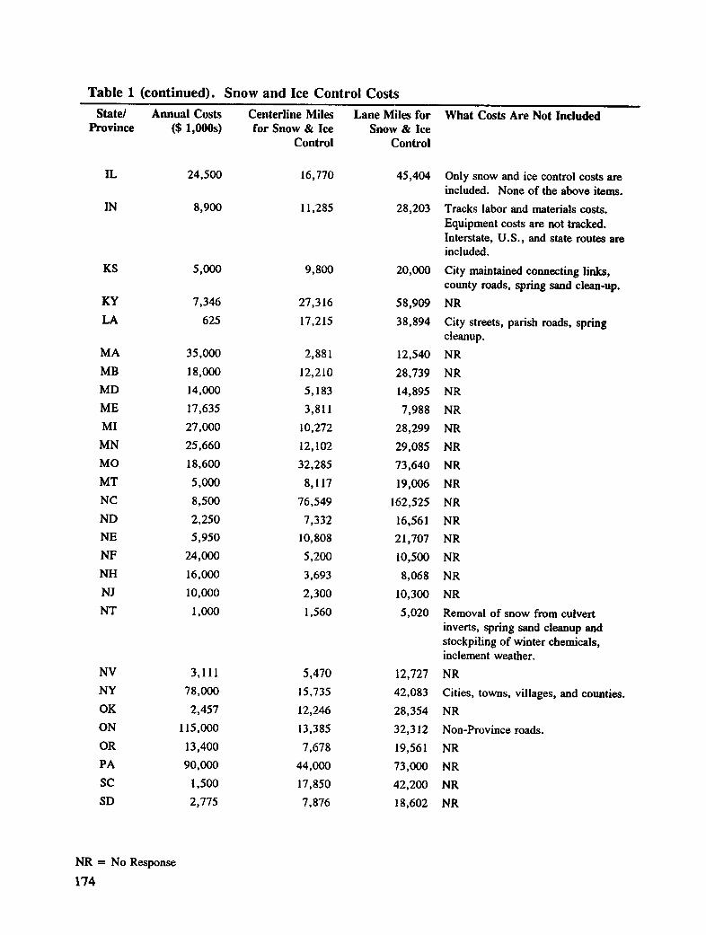
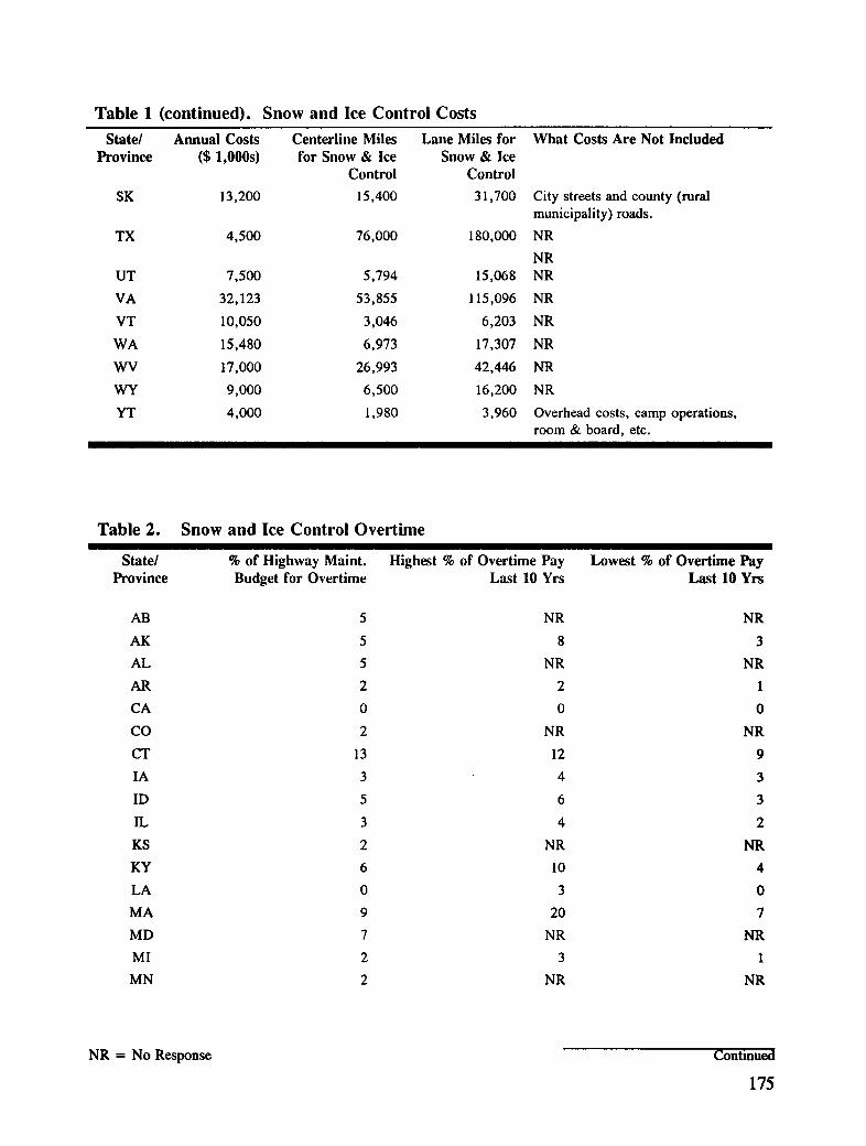
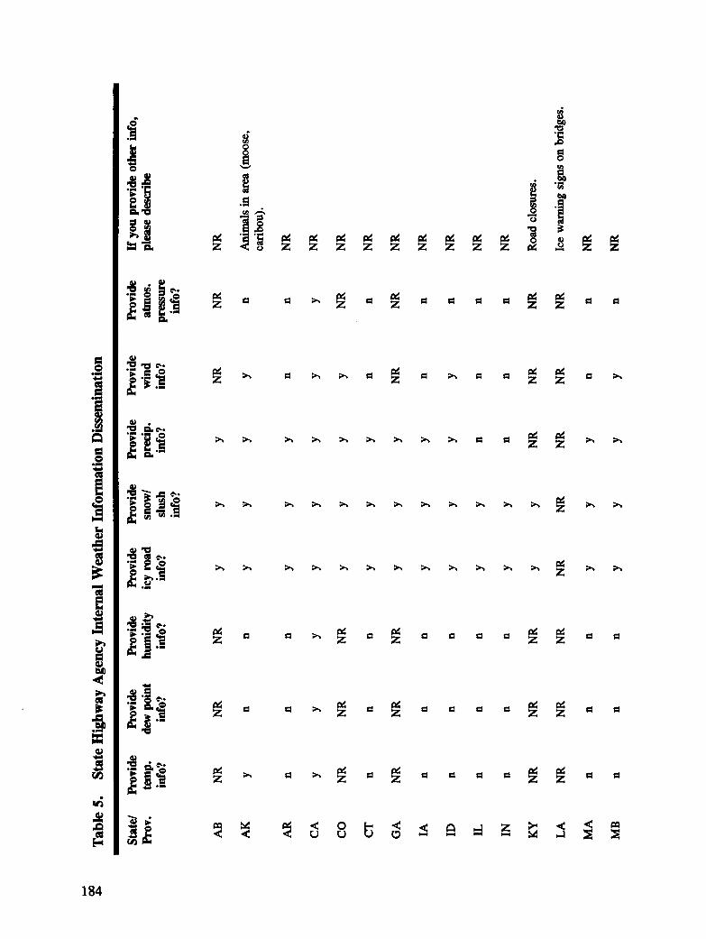
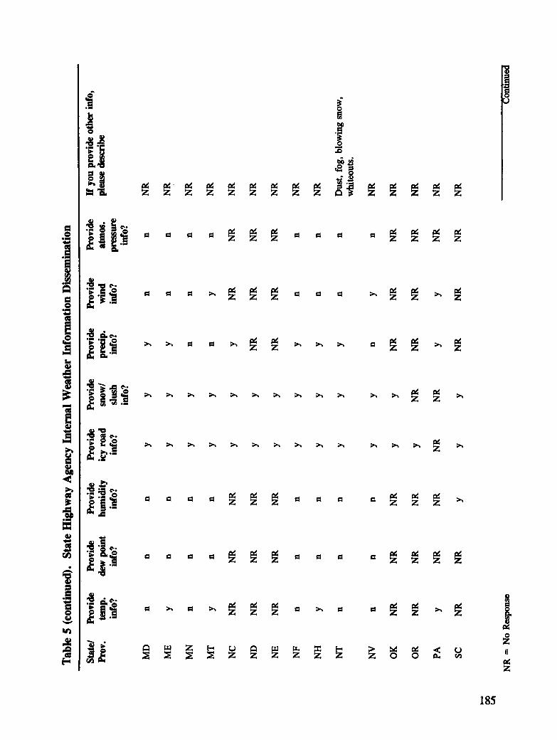
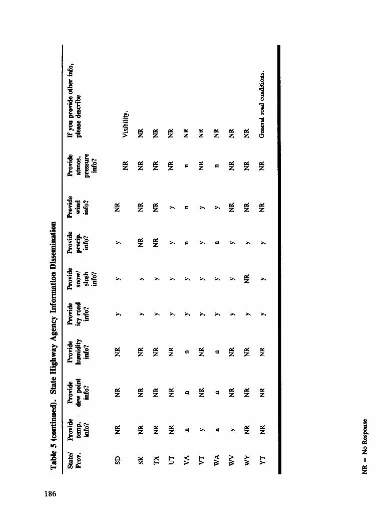
In order to determine the extent of use of RWIS components in support of snow and icecontrol, questionnaires were sent to all state highway agencies and to the provinces ofCanada. In addition, information was sought on the range of snow and ice activities used byhighway agencies and the costs of those activities. Responses were received from 82 % ofthe states and provinces. Those that did not respond were contacted verbally to at leastobtain their expenditures for snow and ice control.
State Highway Agencies
The large expenditures for snow and ice control were documented through this survey. Datafrom the survey in 1988 and 1989, plus calls to states which had not responded, indicatedthat states and Canadian provinces spend over $1.5 billion per year in this area. In addition,1987 Federal Highway Administration (FHWA) data showed that $700 million more is spent
18
by cities and counties in the United States for snow and ice control (U.S. Department ofTransportation, FHWA 1987).
In addition to obtaining cost data, the survey documented the use of various RWlStechnologies. This information was used to find agencies which were willing to participate ina formal evaluation of their technologies. These technologies include actual or plannedinstallations of RWlS observing systems, uses of forecast support, actual or planned roadthermal analysis, or unique installations which could be used to answer key questions relatedto the siting of observing systems.
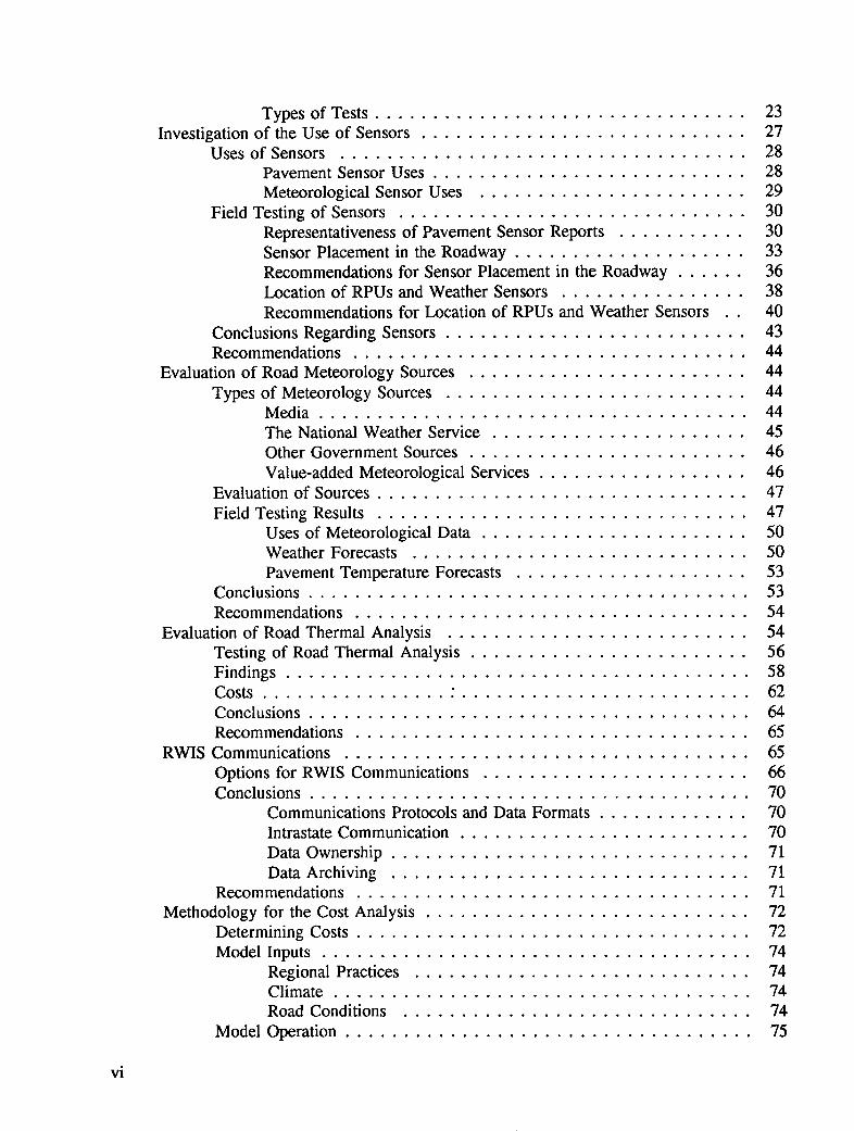
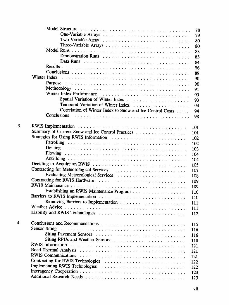
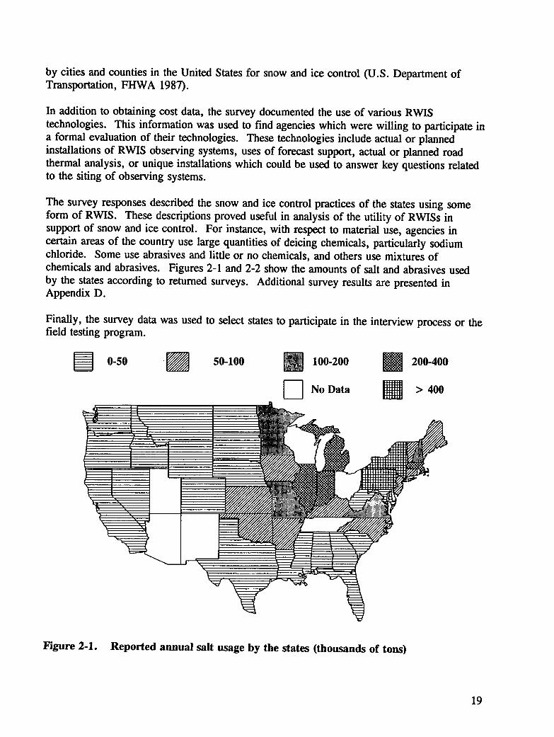
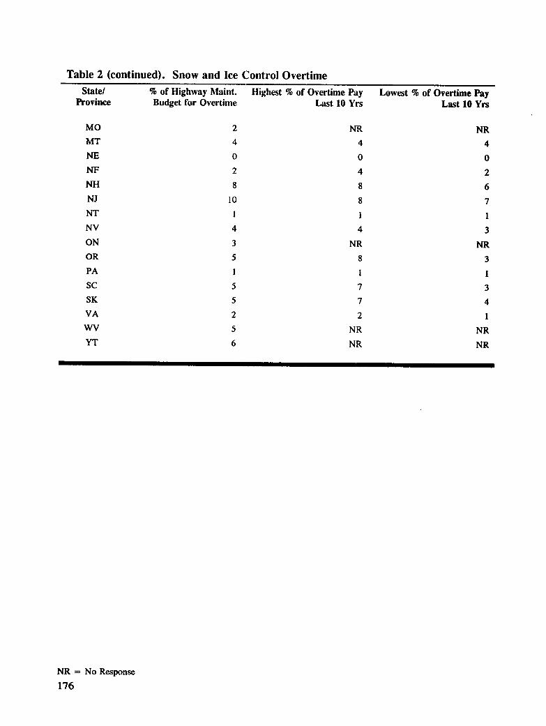
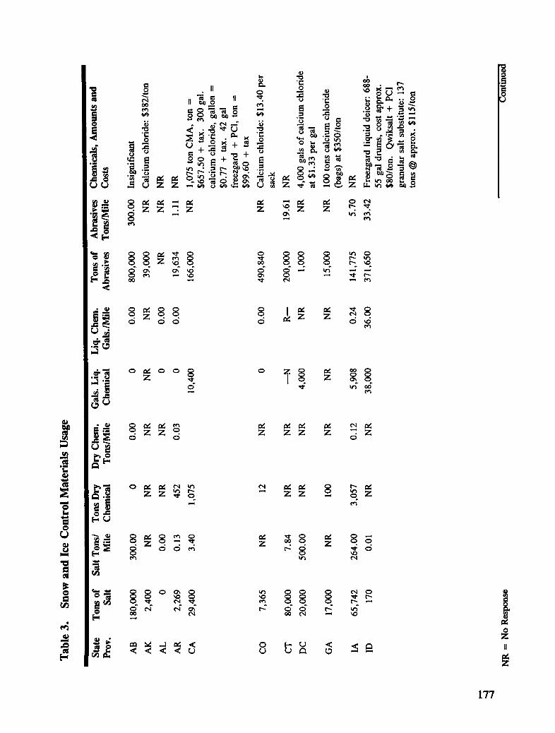
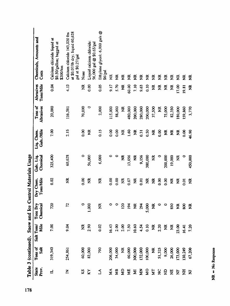
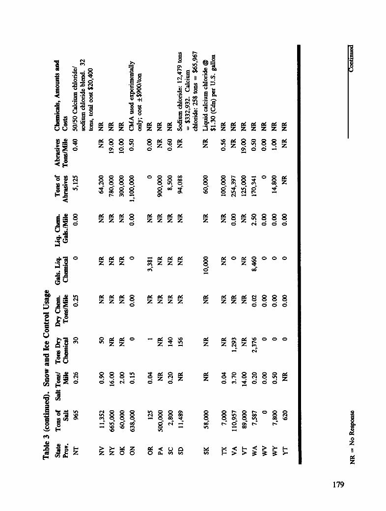
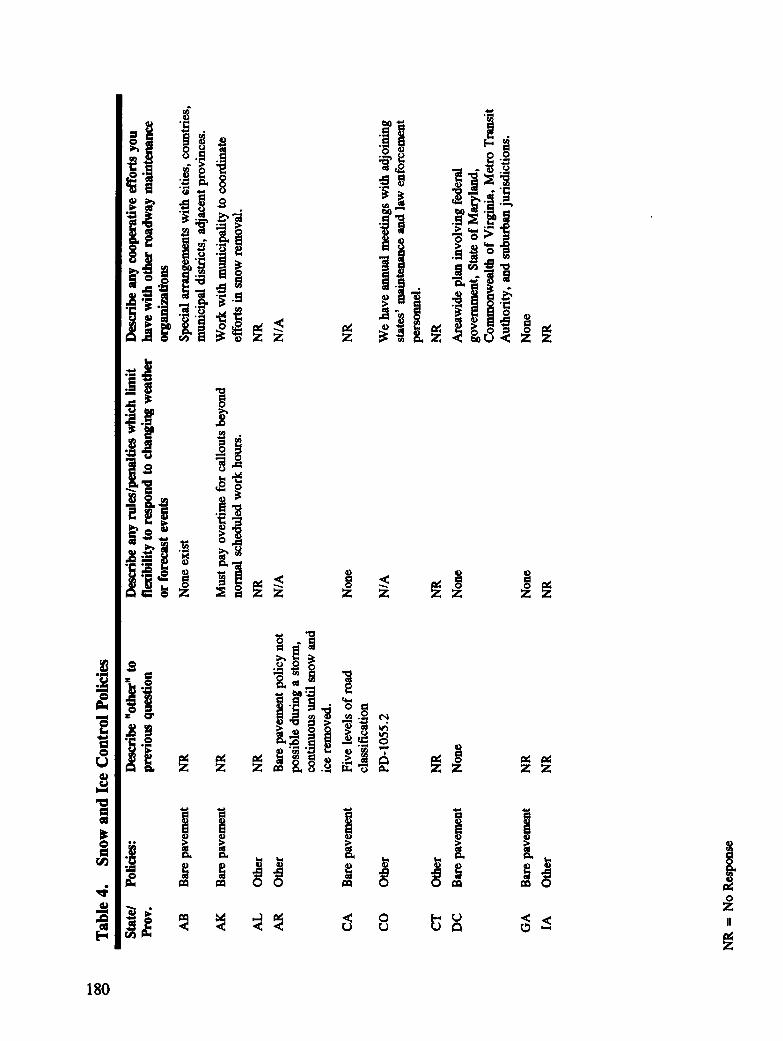
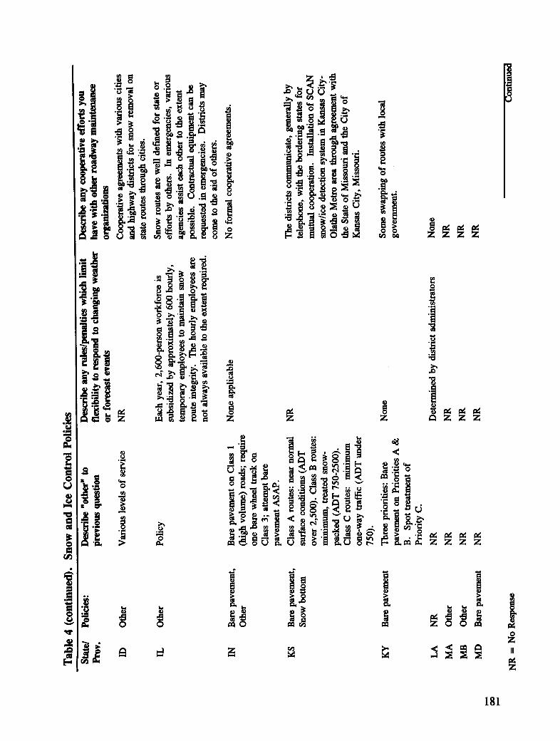
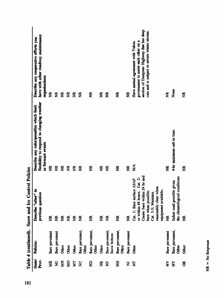
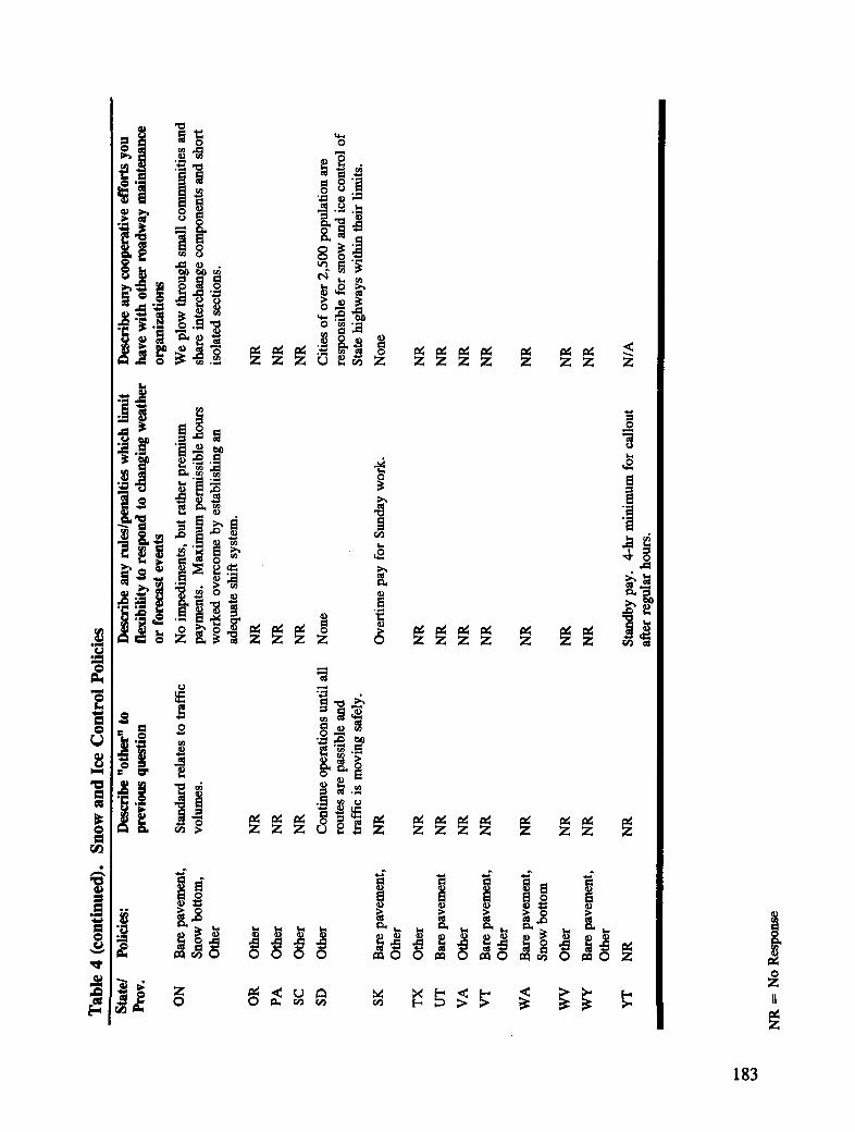
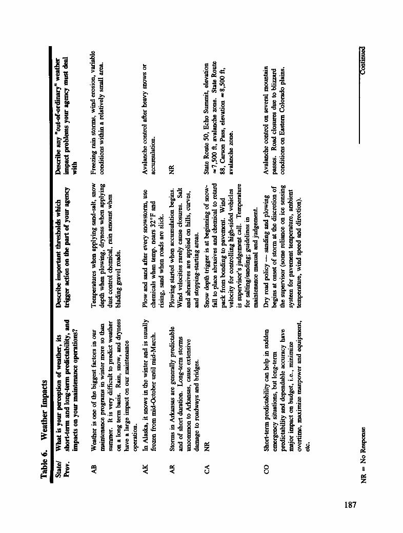
The survey responses described the snow and ice control practices of the states using someform of RWlS. These descriptions proved useful in analysis of the utility of RWISs insupport of snow and ice control. For instance, with respect to material use, agencies incertain areas of the country use large quantities of deicing chemicals, particularly sodiumchloride. Some use abrasives and little or no chemicals, and others use mixtures ofchemicals and abrasives. Figures 2-1 and 2-2 show the amounts of salt and abrasives usedby the states according to returned surveys. Additional survey results are presented inAppendix D.
Finally, the survey data was used to select states to participate in the interview process or thefield testing program.
0-50 _ 50-I00 I I00-200 _] 200-400
_-_ NoData _ >400
Figure 2-1. Reported annual salt usage by the states (thousands of tons)
19
-_ No Data [_ > 400
Figure 2-2. Reported annual sand usage by the states (thousands of tons)
Meteorological Hardware and Services Vendors
Questionnaires were also sent to vendors of meteorological and pavement sensing orobserving equipment and to private providers of meteorological services. Questions wereasked on topics which ranged from the types of forecasting support provided and accuraciesof forecasts to the performance specifications of hardware. In general, the privatemeteorological community was unwilling to divulge information because of concerns overproprietary issues. Some vendors that did provide detailed information requested that theinformation be treated confidentially. Most of the information related to hardware wasprovided in advertising materials.
Interviews
Inte_iews were conducted with state highway agency snow and ice control managers anddecision makers and with vendors of RWIS components. The primary purposes of theinterviews were to determine the extent of in-place RWIS hardware and how pavement
sensors were being used, to assess how weather information was communicated within oroutside state highway agencies and how it was being used, and to determine if a statehighway agency would be willing to participate in the field trials.
20
State Highway Agencies
These interviews thoroughly discussed state highway agency snow and ice control programsand their uses of labor, equipment, and materials. This topic was explored in order todetermine what effect RWISs could have on their operations.
Ten statesmMassachusetts, New Jersey, Pennsylvania, Michigan, Minnesota, Missouri,Colorado, Wyoming, Washington, and Alaskamwere chosen for interviewing. Wisconsinwas added later. In addition, interviews were conducted in British Columbia, Canada.These states and British Columbia were chosen because they were using or planned to usesome RWIS components, represented a cross-section of different snow and ice controlpractices, and had varied climates. Also, British Columbia's highway ministry had recentlycarefully documented its maintenance procedures because of an initiative to privatize allhighway maintenance, including snow and ice control, and it had some in-housemeteorological support. Finally, RWIS uses may vary among state highway agenciesaccording to their different snow and ice control practices and the types and frequencies ofwinter weather events they experience.
In all cases, interviews were conducted at every level of snow and ice control management.Initial interviews were usually held with state or district headquarters managers. From thatpoint, interviews were arranged and conducted with supervisors who made the decisions toimplement snow and ice control activities. Follow-on interviews were also held in most ofthese states to talk in detail about snow and ice control practices and to discuss possible fieldtesting.
Vendors
Informal discussions were also held with vendors of RWIS components to establish aframework of cooperation in the conduct of this research. An evaluation of each vendor'sproducts was never the intent of the research. The purpose of the research was to determinethe utility and cost-effectiveness of the technologies. Operating with those ground rulesfacilitated the exchange of information between the project team and the vendors.
Field Tests
Although the data gathering and interviewing of snow and ice control personnel providedgreat insight into the current and potential uses of RWIS, a number of critical questionsremained unanswered. These included:
• What meteorological parameters are critical in support of snow and ice controldecisions and should therefore be measured?
• What are the optimum heights for weather sensor installations, in particular, windspeed and direction and relative humidity (dew point)?
21
• Where should weather and pavement sensors be placed along the roadway, i.e., howfar apart should sensors be placed and how many are needed to give representativedata?
• Where should pavement sensors be placed in the roadway in relation to the centerline,e.g., in a through lane or a passing lane?
• Should pavement sensors be placed in wheel tracks, lane center, or between lanes?
• What types of weather forecasting services can best serve highway maintenanceagencies?
• What are the benefits and costs of the weather information options available tohighway maintenance agencies?
These questions could best be answered by conducting field tests. Data gathered from in-place sensor systems and from highway maintenance agencies were analyzed to document theanswers to the above questions and to determine costs.
Participants
Initially, three states were selected to participate in the field testing program for H-207:Minnesota, Colorado, and Washington. These states were selected because they are locatedin different climates, they have very different snow and ice control practices, and each hadelected to test some forms of RWIS technology.
• The Minnesota Department of Transportation had installed one make of sensor in theMinneapolis area, installed a second make at its research facility near Monticello(Mn/ROAD) which could be used in analyzing variations in pavement temperaturesacross lanes of traffic, installed a third make and contracted for road thermographicand climatologic analysis in Duluth, had contracted for weather forecasting services tosupport snow and ice control managers, and had hired a meteorologist as a staffweather advisor.
• The Colorado Department of Transportation had installed a large number of sensorsin the Denver area which could be used for analysis of the spatial variability oftemperatures and requirements for numbers of sensor sites, and had contracted forweather forecasting services.
• The Washington Department of Transportation had contracted for road thermographicanalysis and installed sensors in the Seattle area, had contracted for weatherforecasting services for a number of areas in the State, and had participated in aunique, multiagency RWIS sensor system installation in the Spokane area.
22
It was believed that the combinations of weather technologies, practices used for snow andice control, and different climates provided by these states would give sufficient informationfor answering the questions posed above. However, insufficient winter weather could occurin one or more of these locations. To preclude lack of data, four additional states werecontacted to assist in data gathering: Massachusetts, New Jersey, Michigan, and Missouri.Each of these states had acquired and was testing or using some form of RWIS technology:
• Massachusetts had installed 16 pavement sensors in the Braga Bridge in southernMassachusetts. The bridge is high and long, prone to icing, and subject to varyingsurface conditions depending on the weather. The state also contracted with aweather forecasting service for snow and ice control assistance.
• New Jersey was one of the first states to install pavement and weather sensors, andbased on in-house research, intended to expand its initial system located in southernNew Jersey to other regions in the state, and had contracted for weather forecastingservices.
• Michigan had installed sensors in the Lansing and Saginaw areas, the latter on theZilwaukee bridge where they were also using only an alternative deicer.
• Missouri, in cooperation with the City of St. Louis, had installed a sensor system inEureka. Missouri also installed RWIS technology in the Kansas City area.
Types of Tests
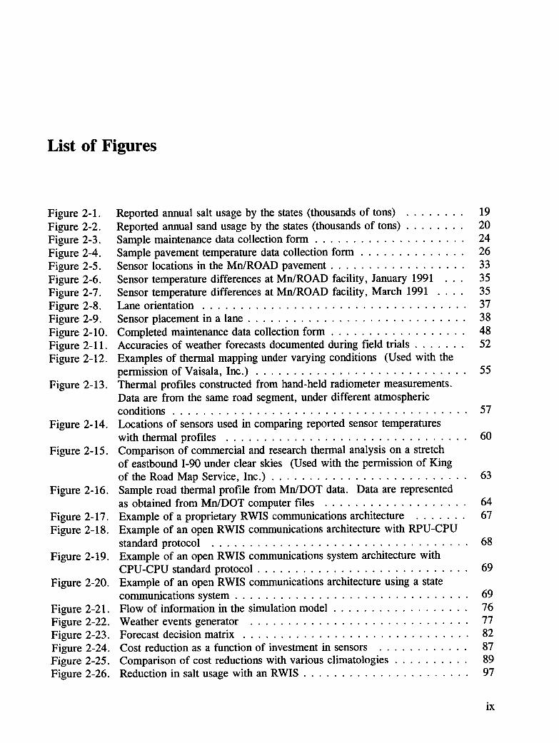
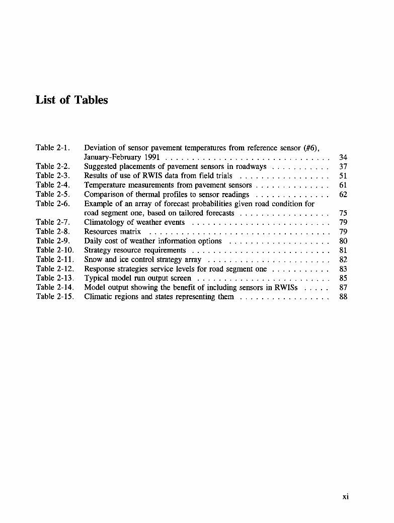
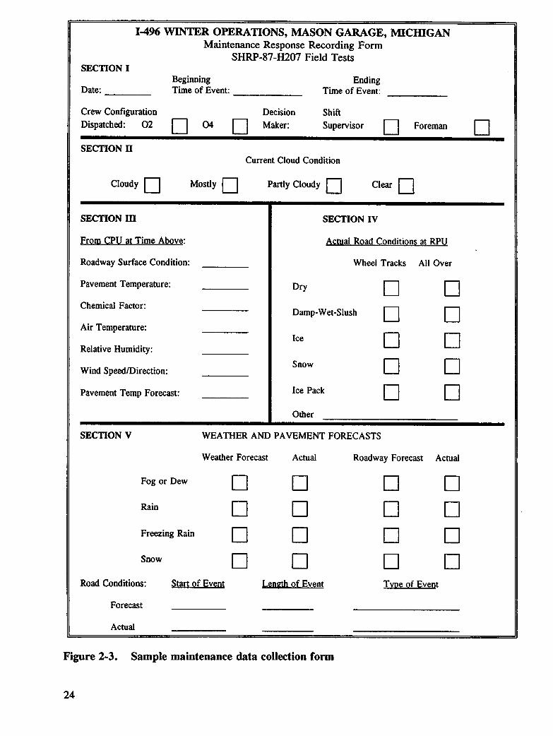
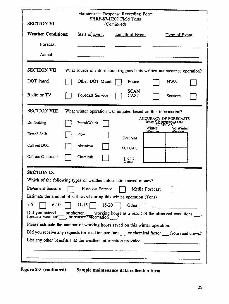
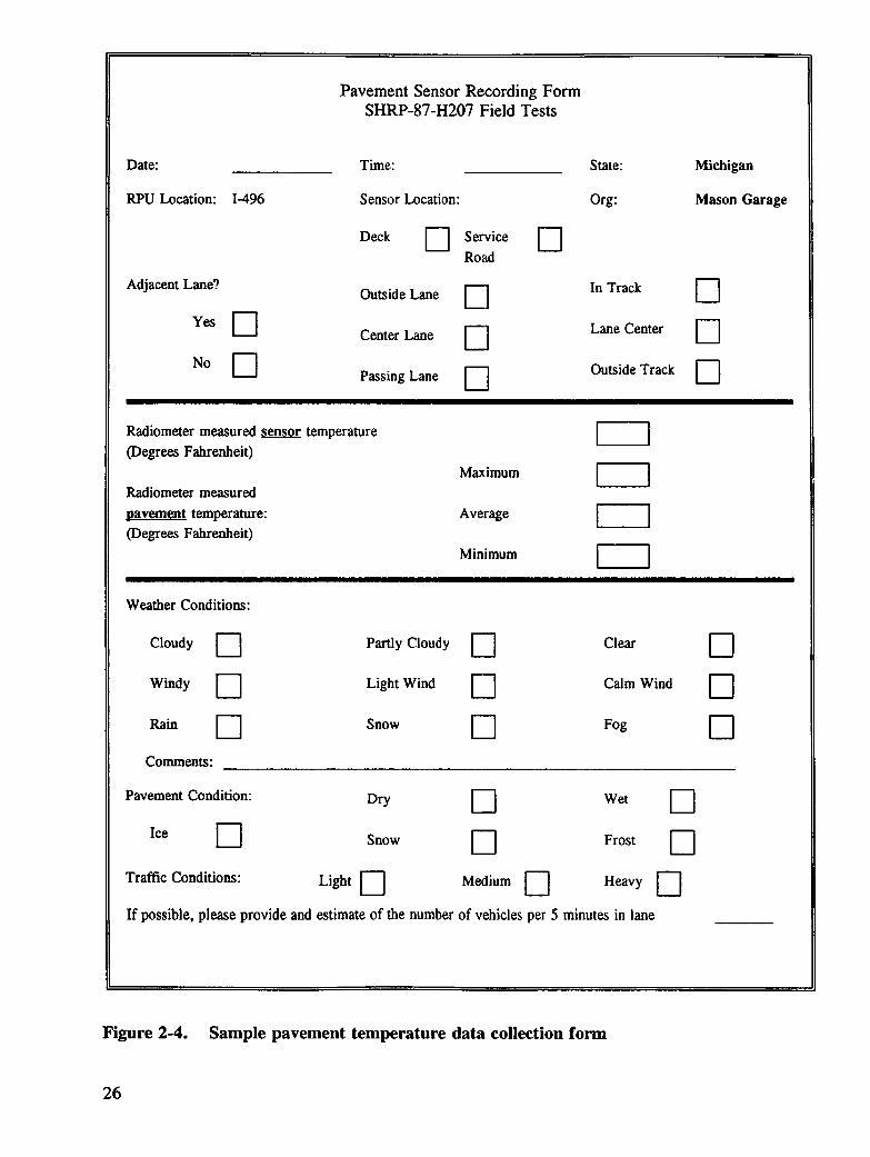
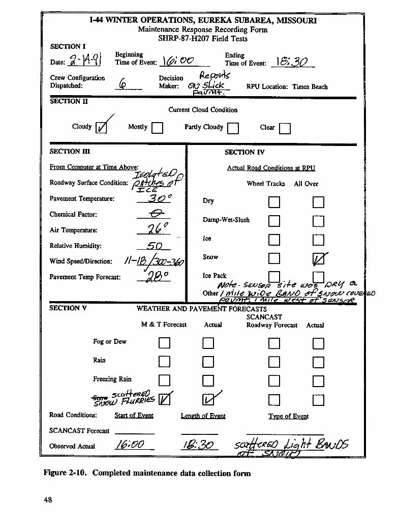
Three types of data were gathered with the assistance of the seven participants. First, theparticipants were asked to assess the utility of available weather information in makingdecisions and to document any cost savings (Figure 2-3). Forms were tailored to eachmaintenance unit participating. For example, the SCANCAST shown in Section VII ofFigure 2-3 is forecast support provided to Michigan DOT by Surface Systems Incorporated."Second, the participants were asked to make pavement temperature and atmosphericmeasurements using a hand-held infrared radiometer and portable air temperature/relativehumidity instrument in order to determine the representativeness of temperatures measuredby pavement sensors and atmospheric sensors (Figure 2-4). Finally, the three original teststates were asked to provide diskettes of data acquired from in-place sensors which wereused as follows:
• Data from an installation of eight pavement temperature sensors placed in four trafficlanes at the Mn/ROAD research facility near Monticello were used to help determinewhere temperature sensors should be placed in the road.
• Data from 14 different locations in the Denver urban area were used to analyze thenumber of sensors required to provide sufficient information for an area.
* The mention of a brand name does not constitute endorsement of that product.
23
1-496 WINTER OPERATIONS, MASON GARAGE, MICHIGANMaintenance Response Recording Form
SHRP-87-H207 Field TestsSECTION I
Beginning EndingDate: Time of Event: Time of Event:
Crew Configuration Decision Shift
SECTION HCurrentCloud Condition
Cloudy [--] Mostly D PartlyCloudy [-"] Clear ["-]
SECTION HI SECTION IV
From CPU at Time Above: Actual RQadConditiQn_at RPU
RoadwaySurfaceCondition: Wheel Tracks All Over
PavementTemperature: Dry D D
Chemical Factor: Damp-Wet-Slush [--] [-7Air Temperature:
I. [3 NRelative Humidity:
Wind Speed/Direction: Snow D D
Pavement Temp Forecast: Ice Pack D D
Other
SECTION V WEATHERAND PAVEMENTFORECASTS
Weather Forecast Actual Roadway Forecast Actual
_o_o_ow f-1 [Z 77 17Rain D D D D
Freezing Rain ['"l _-] D ["]
_oo_ D 7-1 D DRoad Conditions: Startof Event Lenmhof Event Tyne of Event
Forecast
Actual
Figure 2-3. Sample maintenance data collection form
24
Maintenance Response Recording FormSHRP-87-H207 Field Tests
SECTION VI (Continued)
Weather Conditions: _ _ Type of Event
Forecast
Actual
SECTION VII What source of information triggered this written maintenance operation?
DOT Patrol D Other DOT Maint D Police D NWS D
SCAN
Radio or TV D Forecast Service D CAST D Sensors
SECTION VIII What winter operation was initiated based on this information?
ACCURACY OF FORECASTS
Do Nothing [-'7 Patrol/Watch _'q (place X in appropriate box)FORECASTI........,,,..J I..-..I
Winter No WinterWF._thar Wpath_l-
Extend Shift D Plow D Occurred
Call out DOT D Abrasives D ACTUAL
Call out Contractor _ Chemicals D Didn'tOccur
SECTION IX
Which of the following types of weather information saved money?
Pavement Sensors D Forecast Service [-7 Media Forecast D
Estimate the amount of salt saved during this winter operation (Tons)
1-5 ['-'] 6-10 D 11-15[_] 16-20 D Other D
Did you extend or shorten __ working ho s as a result of the observed conditionsforecast weather , or sensor reformation ur.
Please estimate the number of working hours saved on this winter operation.
Did you receive any requests for road temperature or chemical factor from road crews?
List any other benefits that the weather information provided.
Figure 2-3 (continued). Sample maintenance data collection form
25
Pavement Sensor Recording FormSHRP-87-H207 Field Tests
If possible, please provide and estimate of the number of vehicles per 5 minutes in lane
Figure 2-4. Sample pavement temperature data collection form
26
• Data from three sensor installations in the Seattle area were used to compare withroad thermography data to assess the validity of the road thermography.
The field tests were conducted in all locations from October 1, 1990 through March 31,1991. In order to establish a common framework for the testing, a meeting was held withthe participants in each state to provide guidance on how to fill out the forms and how to usethe measuring instruments. Ground rules for obtaining measurements were discussed. Forinstance, in order to make the workload manageable for the state highway agencies, andsince freezing is a critical highway consideration, the state highway agencies were asked toobtain pavement temperature measurements when the pavement temperature was expected togo to or below 32°F (0°C). The state highway agencies were told that safety of workers hadto be the foremost concern, and if conditions in the road environment were too dangerous,
e.g., not enough spacing between vehicles to ensure being able to obtain pavementtemperature measurements safely, then measurements should not be taken. The Manual ofUniform Traffic Control Devices (MUTCD) was to govern in all cases with respect toneeded traffic control.
In addition to the data collection by the state highway agencies, the research team conductedits own field tests. Initially, these tests were conducted primarily to gather radiometricpavement temperature data to determine the validity of road thermography which had beenconducted in Minnesota and Washington. However, after some early measurements by statehighway agencies with the hand-held infrared radiometers indicated that there were somediscrepancies between sensor temperature reports and the radiometer reports, additionalpavement temperature measurements were taken by the research team and the state highwayagencies in order to try to assess the magnitude of likely errors. Details are discussed in thefollowing section, "Investigation of the Use of Sensors."
Finally, after more than one state observed these temperature discrepancies, the vendors ofpavement sensors were notified. SSI undertook a detailed investigation of the use of thehand-held radiometer to measure pavement temperatures. The results of their investigationpointed to problems in using the radiometer. It also indicated that the radiometer could beused for measuring pavement temperatures under carefully controlled circumstances andwhen used in a specific manner by a knowledgeable user (SSI 1991). Guidance is providedin the following section.
Investigation of the Use of Sensors
There were two major objectives in investigating pavement and meteorological sensors. Thefirst was to determine their current and potential uses. The second was to determine wheresensors should be placed in the roadway and how many of them are needed in an area.
27
Uses of Sensors
The following descriptions of the uses of sensors are based on information gathered primarilyfrom the interviews. The field tests did provide some additional insight, although they weredesigned to address more specifically the issues related to the siting of sensors.
Pavement Sensor Uses
There are two kinds of pavement sensors, in situ or in-place sensors, and remote sensors.Examples of in situ pavement sensors include simple thermistors or thermocouples installedin a road surface to measure pavement temperature. More sophisticated in situ devicesprovide surface temperature, indications of the concentration of deicing chemicals on theroad, and an indication of the state of the surface, e.g., whether it is wet or icy. Becausethey provide a great deal of information, these sensors can have a number of uses.
Remote sensors provide information from some distance. Weather radar is an example of aremote weather observation. Research is being conducted in Europe on the use of remotemicrowave sensors installed along roadways to determine pavement temperature and surfaceconditions. Such observations may prove very useful because in situ measurements representonly a very small surface area, on the order of tens of square centimeters, compared toremote measurements of tens of square meters. The latter observations may be morerepresentative of the road environment than those obtainable from the smaller in situinstruments.
Sensors can also be active or passive. The in situ sensors discussed above are passive.Changes in their electrical properties are used to determine the temperature or condition ofthe road surface. Active sensors have now been developed: a freezing-point sensor actuallycools a surface to determine at what temperature moisture on the surface will freeze, thenheats it to repeat the measurement cycle. This information is potentially more valuable thanpavement temperature alone since it will measure the effects of any deicing chemical present.If the freezing point is known, then a forecast of minimum pavement temperature can beused to determine whether a surface will freeze.
Pavement sensors are used for three purposes: detecting, monitoring, and predicting.
• First, they are used to detect critical conditions or the attainment of critical thresholdsfor decision makers. They serve an alerting function. For example, alerts includethe surface temperature reaching 32°F (0°C), the presence of moisture, or the
occurrence of precipitation. Each of these can be a critical piece of information onwhich a manager wish¢s to take action, or at least be notified. Without sensors, suchnotification must come from observations from highway crews, police, or thetraveling public. Unfortunately, many times, the notification comes from the policeproviding "constructive knowledge" of a situation that requires attention because anaccident has occurred and the highway agency must take action. Some highway
28
agencies use road patrols to detect critical conditions, but this turns out to be a costlyalternative.
• Second, pavement sensors can be used to monitor current conditions. Althoughmonitoring and detecting may be similar, detecting is associated with alerting andreacting. Monitoring sensor output allows a manager to assess the progress ofweather conditions or snow and ice control activities. A pavement sensor providesthe ability to monitor road temperatures and compare them to forecasts, to monitorroad conditions "upstream" in the weather pattern or prior to a weather change, toassess the progress of weather as road conditions change, and even to assess theprogress of maintenance work. For example, a pavement sensor that measures theconductivity of the surface, i.e., the amount of deicing chemical present, providesinformation to a manager concerning whether chemicals should be applied, or evenwhen they were applied. There were situations revealed in the interviews wheresupervisors had cross-checked maintenance logs against pavement sensor data todetermine when chemicals were applied on a specific route. Also, such data becomea valuable resource for documenting maintenance actions if faced with liability claims.
• The third use of pavement sensors is for prediction. The most savings in snow andice control will come from maintenance managers making timely and effectivedecisions about snow and ice control activities. To do this, managers need to knowwhat conditions are expected. One of the important forecast parameters is pavementtemperature. A critical input into pavement temperature forecast models is subsurfacetemperature. A subsurface temperature probe assists in forecasting surfacetemperatures. A surface temperature sensor also allows for fine-tuning or updatingsurface temperature forecasts.
Meteorological Sensor Uses
Meteorological sensors can also be used for detection, monitoring, and prediction purposes.
• For ice detection purposes, the dew point is critical. If the pavement surfacetemperature falls below the dew point, moisture will condense on the pavement. Ifthe ambient temperature is less than or equal to the freezing point of the road surface,then ice or frost will form on the pavement. The dew point measurement thenbecomes part of the detecting/alerting system.
• Meteorological sensors also play a large role in monitoring current conditions.Although the pavement temperature is important, monitoring the weather conditionsupstream or downstream helps in the decision to initiate or suspend maintenanceactions. For example, in areas of prevailing westerly winds, data from an RPU to thewest can be the first indication that predicted weather will or will not occur. Aprecipitation detector might sense the first snowfall. Temperature drops and windspeed and direction changes can indicate that a weather system is progressing. In
29
other areas, monitoring the wind speed and direction may provide clues to what kindof road conditions will occur and what maintenance activities may be needed.
• Meteorological sensors also aid in predicting road and weather conditions. Accurateforecasts require knowledge of current conditions. Wind, temperature, and moisturepatterns determine what will take place in terms of weather and road conditions. Aweather forecaster who has meteorological data available will make a more informedand accurate forecast. The data can also be used for special studies of weatherphenomena to improve forecasting. Such "local forecast studies" are extremelyvaluable in improving forecast capability.
Field Testing of Sensors
Several field-tests of sensors were conducted. These dealt with the representativeness ofpavement sensor reports, optimum sensor placement in the roadway, and locating RPUs andweather sensors along roadways.
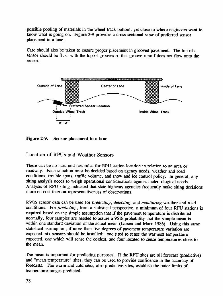
Representativeness of Pavement Sensor Reports
The states and the research team gathered data using hand-held radiometers to determinepavement sensor report representativeness. It was decided to use infrared pavementtemperature measurements because contact devices require too much time to be used safely inmany of the highway test locations. Sensors at selected RPU locations were to be checkedwhenever the temperature reached 32°F (0°C). This temperature was selected becausesensors should be most representative when the surface temperature is near freezing. Eachstate highway agency was provided a Raytek PM-4 ° radiometer to take pavementtemperature measurements. A radiometer indicates the temperature of a surface in terms ofits infrared radiation; the readout is directly in degrees Fahrenheit (°F) or degrees Celsius(°C). The state crews were instructed to point their radiometers vertically at sensors in thepavement to measure their temperature. Then the radiometers were pointed at the pavementsurrounding the sensors, and the average, maximum, and minimum temperatures wererecorded. Finally, and if conditions permitted, the average, maximum, and minimumtemperatures from an adjacent lane were recorded. Records of the pavement temperaturesensor outputs were also annotated. All measurements were documented in °F.
Temperature Reporting Accuracy. It was never the intent to check the accuracy ofindividual pavement temperature sensors. However, it soon became apparent that somediscrepancies existed. The first two state highway agencies to receive their radiometersfound that they were frequently getting radiometer-reported pavement temperatures 5-7°F(3-4°C) lower than the sensor-reported temperatures. The research team conducted its owninvestigation using a site in Washington State and found the same discrepancy. The team
* The mention of a brand name does not constitute endorsement of that product.
30
had also used a contact probe as a backup, and this confirmed the discrepancy. Subsequentmeasurements by the research team using another vendor's sensors produced the samediscrepancy. This indicated that there was more of a problem with temperature reportingthan just whether sensor temperatures were representative of road temperatures.
There are a number of reasons why this discrepancy can occur.
• A sensor is thermally isolated from the pavement by the mastic used to cement thesensor into the pavement.
• The backfill materials under a pavement sensor may change the thermal flux beneathit.
• A subsurface sensor may be installed beneath a surface sensor providing a thermalconduit below the latter different from adjacent pavement.
• A sensor exterior is thermally different than the pavement due to its construction andmaterials.
• The thermal characteristics of an entire sensor, including its electronic components,are different from those of pavement.
Each of the three major vendors of pavement temperature sensors was notified that thesediscrepancies had been observed. The team was informed by one manufacturer that thesensor was designed to report "accurately" when the road surface condition is wet and thesky condition is either cloudy or dark. This was a conscious decision by the manufacturerbecause it believed that wet and dark/cloudy conditions presented the worst situation forsnow and ice control decision makers.
Under sunlit conditions and dry pavement, these sensors may register temperatures higherthan the surrounding pavement. This means that for frost or black-ice situations, pavementtemperature sensors may report temperatures too high. However, under some sunnyconditions and wet pavement, or even recently wet appearance, these sensors can reportpavement temperatures accurately.
Sensor Calibration. It is sometimes impossible to tell how representative pavement sensorreadings are of the pavement temperature because in general, there is no record of sensorcalibration after installation. The discrepancies discussed above can only be described inrelative terms because of a lack of knowledge of actual sensor maintenance. Based on theSSI evaluation of the Raytek PM-4 radiometer, Mr. Robert Hart (personal communication,1991) suggest that a procedure could be developed to use such an instrument to calibratesurface temperature sensors.
Radiometer Use. Some of the temperature discrepancies noted earlier may have been due toproblems in using the radiometer. Problems arise from:
31
• Taking a warm radiometer into the cold exterior environment and inducing it tothermal shock. All participants were asked to keep their radiometers in a cold vehicletrunk or pickup bed. If that were not possible, the instruments were to be placedoutside in the cold to stabilize. The research team's radiometer was always stored ina trunk overnight before measurements were taken.
• Measurements taken too high above the pavement. A detailed investigation conductedby SSI Showed that the Raytek radiometer was accurate if placed just at the pavementsurface (SSI 1991). Temperature differences of up to 2°F (1 °C) were introduced byholding the radiometer 20 in. (0.5 m) above the pavement." For absolutetemperature measurements, this could be a problem. For relative differences, itshould not be. All participants were instructed to take measurements at knee heightto obtain relative measurements.
Based on the research conducted by SSI and the research team, the following generalinstructions should be followed when using a radiometer to measure surface temperatures:
• Always keep the radiometer in a cold environment, such as the trunk of a vehicle, inorder to minimize the thermal shock the instrument will experience if moved from awarm environment to cold. Thermal shock produces erroneous readings.
• If the instrument cannot be stored in a cold place, when arriving at a measurementsite, place the instrument outside but not exposed to solar radiation for at least 30minutes to allow it to cool to ambient temperature.
• Take a measurement by holding the radiometer vertically 1 in. (about 2-3 cm) abovethe pavement. Resting the instrument on the toe of a shoe and pointing it at thesurface provides a reasonably consistent method of measurement.
• Take measurements before sunrise to avoid solar radiation entering the instrument.
• Take at least four temperature measurements at each location. Compute the samplemean and standard deviation of the measurements. The sample standard deviationshould be less than the error of the instrument (as specified in the manufacturers'literature).
The radiometers were acquired to collect relative temperature measurements, and todetermine the representativeness of sensor measurements of the roadway temperature.Experience with the radiometers suggests that careful procedures need to be established fortheir use, they should be used by trained personnel, their measurements should not beconsidered absolute, and they should be calibrated carefully.
* The research team was not able to verify the discrepancy positively. The SSI measurements were takenusing a radiometer and a thermistor implanted in the pavement. Research team measurements were takenusing a radiometer and a contact probe. Differences of up to 20F (I'C) were noted when takingmeasurements at about 20 in. (0.5 m) and 1 in. (2-3 em) above pavement. However, the two-degreedifference is within the combined errors of the two instruments.
32
Data Reporting Frequency. It is very difficult to verify data from pavement sensors that donot provide data on a regularly-scheduled basis. In most RWISs, if no critical thresholds arecrossed, no data are reported. This condition can exist for hours. A data user is unable totell if there are no data reports because of no change or because of malfunctions. The valuesof parameters such as surface temperature can only be estimated during this condition.
Sensor Placement in the Roadway
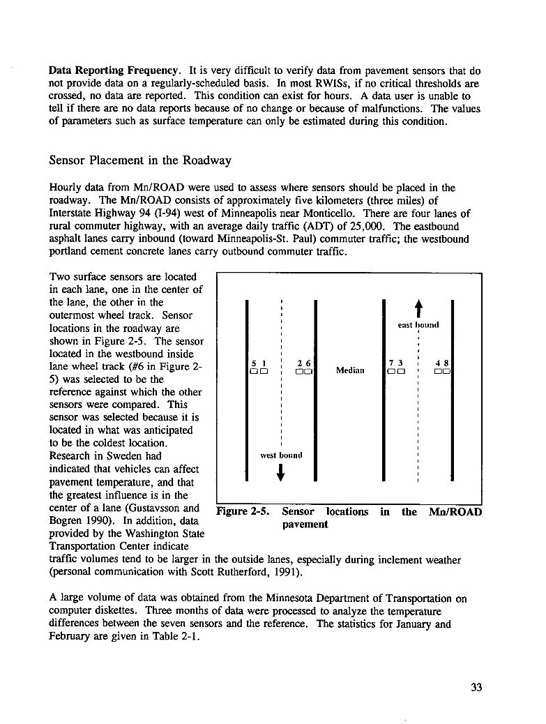
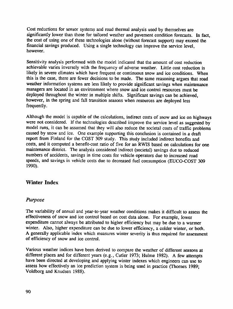
Hourly data from Mn/ROAD were used to assess where sensors should be placed in theroadway. The Mn/ROAD consists of approximately five kilometers (three miles) ofInterstate Highway 94 (I-94) west of Minneapolis near Monticello. There are four lanes ofrural commuter highway, with an average daily traffic (ADT) of 25,000. The eastboundasphalt lanes carry inbound (toward Minneapolis-St. Paul) commuter traffic; the westboundportland cement concrete lanes carry outbound commuter traffic.
Two surface sensors are locatedin each lane, one in the center of
the lane, the other in the &,outermost wheel track. Sensor /
locations in the roadway are eastboundshown in Figure 2-5. The sensorlocated in the westbound inside
lane wheel track (#6 in Figure 2- 5 ! 2 6 7 3 4 8O 0 1=30 Median O O Dr-a5) was selected to be thereference against which the othersensors were compared. Thissensor was selected because it is
located in what was anticipatedto be the coldest location.Research in Sweden had west bound
indicated that vehicles can affect .l.pavement temperature, and thatthe greatest influence is in the
center of a lane (Gustavsson and Figure 2-5. Sensor locations in the Mn/ROADBogren 1990). In addition, data pavementprovided by the Washington StateTransportation Center indicatetraffic volumes tend to be larger in the outside lanes, especially during inclement weather(personal communication with Scott Rutherford, 1991).
A large volume of data was obtained from the Minnesota Department of Transportation oncomputer diskettes. Three months of data were processed to analyze the temperaturedifferences between the seven sensors and the reference. The statistics for January andFebruary are given in Table 2-1.
33
The statistics indicate that the temperature differences, when averaged over a long period oftime, show little difference, except for sensor #8." However, there were other possibilitiesfor temperature differences that would be masked when considering the long-term averages.Daily fluctuations in traffic and atmospheric phenomena, as well as changes due to pavementconditions (wet, dry, frozen), could also influence the sensor temperatures.
First, the temperatures Table 2-1. Deviation of sensor pavement temperatures fromwere compared by time of reference sensor (#6), January-February 1991day to determine theextent of diurnalinfluences. Because of
the large volume of data, TemperatureDeviation(in *F)observations were Sensor # 1 2 _3 _4 5_ 7_ 8
processed for three-hour Mean difference 0.6 1.1 0.7 0.4 0.6 -0.1 1.2periods from 5:00 a.m. to9:00 p.m. These times Standard deviation 1.1 0.9 0.7 0.8 0.4 0.7 0.8
were selected because Maximum 4.3 5.3 3.7 3.0 2.0 3.8 4.85:00 a.m. covers the cold
Minimum -5.1 -3.7 -1.0 -3.6 -3.4 -2.5 -1.2period before anyinfluence from traffic, Variance 1.2 0.7 0.5 0.7 0.2 0.5 0.78:00 a.m. covers the
morning commuteinbound to Minneapolis-St. Paul, 3:00 p.m. picksup any solar influence, and 6:00 p.m. covers the evening commute. Data for two timeperiods are shown in Figures 2-6 and 2-7.
The data indicate that temperatures in the center of the lanes are warmer than in the wheeltracks, and that traffic volume influences the temperatures. However, it is the experience ofmost snow and ice control people that wheel tracks clear first. This is due to tire grinding,pressure, and friction, which overcome the tendency for the wheel tracks to be cooler. Itshould also be pointed out that these temperatures are measured without snow or ice cover.
In order to relate temperature differences to traffic, volume data were requested fromMn/ROAD. Temperature differences resulting from traffic could not be obtained becauseonly daily ADTs were available; no data were available by hour.
The team also attempted to determine the influence of pavement surface conditions on thetemperatures. Each sensor provided an output indicating whether it was wet or icy. Solarradiometer measurements indicated whether it was clear or cloudy. The pavementtemperature observations were classified into wet, dry and cloudy, and dry and clear cases.
" Separate measurements with a radiometer and a contact probe at the site indicated that sensor #8 wasconsistently reporting temperatures too warm.
F-2"1"50.00t Hour of the day_' _''_'///" ..f/#-2.50
Based on average temperature differences between sensor #6 and other sensors during the period 3/1/91-3/25/91
Figure 2-7. Sensor temperature differences at Mn/ROAD facility, March 1991
35
However, in the middle of January, the sensor system stopped reporting the pavementcondition properly. The vendor was contacted to see if the data could be corrected. Noresponse was received by the end of the field test.
Recommendations for Sensor Placement in the Roadway
Maintenance engineers frequently disagree on precisely where pavement sensors should beplaced in the roadway. Several different options exist which depend on the type of roadsurface, traffic volume, and the purpose of the sensor information.
Pavement sensors are used to predict, detect, and monitor road and weather conditions. Forprediction purposes, sufficient sensor installations are needed to provide reliable informationto whoever is making the road temperature and/or weather forecasts.
Care should be taken to ensure that the slope of a road at any location is such that there is nodrainage onto sensors from the shoulder or the median. Sensors should not be placed in theroadway on curves.
Placement within Lanes. There is also a range of opinions on where sensors should belocated within lanes. Table 2-2 provides a matrix of options for sensor placement withinlanes. Figure 2-8 depicts these locations graphically. Placing sensors for prediction ofpavement temperature and monitoring of forecasts should be the primary criteria. Whendetection of current conditions is desired, installing an additional sensor at a location selectedfor prediction offers the opportunity to obtain both prediction and detection information.
Placing sensors in wheel tracks is another possibility. Wheel tracks tend to get cleaned outby tire friction, and may not be representative of the rest of a roadway. Heavy vehicles suchas trucks can disturb the pavement surrounding a sensor. Also, with significant road surfacewear, water can pool and ice can form first in the wheel tracks. In other circumstances,particularly in high traffic volume areas, wheel tracks can dry out first.
The centers of lanes in urban environments can be affected by vehicle heat. Pavementtemperatures can be as much as 2°F (1 °C) higher in lane centers. Since vehicle heatinfluences pavement temperature, placing sensors in the center of lanes is not recommended.
Another possible location for pavement sensors is between lanes. This area is probably theleast disturbed, but it is also subject to increased concentrations of deicing chemicals anddebris. In addition, sensors here could be accidentally covered with paint during stripingoperations.
36
Table 2-2. Suggested placements of pavement sensors in roadways
Just outside of Just outside of Just outside of a Just outside of aPrediction outside wheel track outside wheel track wheel track of a wheel track of
of outbound of outbound lane passing lane either lanepassing lane
Just inside of Just inside of outside Just outside of a Just outside of aDetection outside wheel track wheel track of wheel track of a wheel track of
of inbound through inbound lane through lane either lanelane
Monitoring Use prediction placement whenever possible
Traffic Flow
/ //
Median Insi_leInsideOutside /.@.,, '_/4"
/
/ // /
/ / Outside/ O" Outside / //
/
Traffic Flow
Figure 2-8. Lane orientation
Placement within Wheel Tracks. There is considerable discussion among highwayengineers as to just where sensors should be placed in wheel tracks. Some prefer the centerof tracks because that is where most of the vehicles run; others prefer just off-center to getout of the bottom of the track. In portland cement concrete surfaces, the precise locationmay not be as crucial as in asphalt because PCC pavements do not generally rut as deeply asasphalt surfaces. Whatever lane is chosen and for whatever purpose, it is suggested thatpavement sensors be placed approximately 8-12 in. (0.2-0.3 m) from a wheel track center.This will keep the sensor away from vehicle influences in the center of the lane, outside the
37
possible pooling of materials in the wheel track bottom, yet close to where engineers want toknow what is going on. Figure 2-9 provides a cross-sectional view of preferred sensorplacement in a lane.
Care should also be taken to ensure proper placement in grooved pavement. The top of asensor should be flush with the top of grooves so that groove runoff does not flow onto thesensor.
Outside Wfieel Track Inside Wheel Track
i 18"-12"
Figure 2-9. Sensor placement in a lane
Location of RPUs and Weather Sensors
There can be no hard and fast rules for RPU station location in relation to an area or
roadway. Each situation must be decided based on agency needs, weather and roadconditions, trouble spots, traffic volume, and snow and ice control policy. In general, anysiting analysis needs to weigh operational considerations against meteorological needs.Analysis of RPU siting indicated that state highway agencies frequently make siting decisionsmore on cost than on representativeness of observations.
RWIS sensor data can be used for predicting, detecting, and monitoring weather and roadconditions. For predicting, from a statistical perspective, a minimum of four RPU stations isrequired based on the simple assumption that if the pavement temperature is distributednormally, four samples are needed to assure a 95 % probability that the sample mean iswithin one standard deviation of the actual mean (Larsen and Marx 1986). Using this samestatistical assumption, if more than five degrees of pavement temperature variation areexpected, six sensors should be installed: one sited to sense the warmest temperatureexpected, one which will sense the coldest, and four located to sense temperatures close tothe mean.
The mean is important for predicting purposes. If the RPU sites are all forecast (predictive)and "mean temperature" sites, they can be used to provide confidence in the accuracy offorecasts. The warm and cold sites, also predictive sites, establish the outer limits oftemperature ranges predicted.
38
This statistical basis for siting may be outweighed by operational needs because of arequirement to monitor trouble spots. Thermal analysis can help locate representativepredictive sites near trouble spots. A site can then become dual-purpose.
In the Denver area, RPU stations are installed at 14 locations with a total of 56 pavementsensors in roadways and bridges. The sites are placed to supply data from all quadrants ofthe urban area. For an analysis of the number of sensors needed in an area, five sensorswere selected to compare to a reference sensor. The six sensors selected were located infour quadrants of the Denver area, plus one near the center of the area.
Data were to be acquired during the period December 1, 1990 through March 31, 1991. TheCPU at the Colorado Department of Transportation became inoperative for a period duringDecember and January. However, the Colorado Department of Transportation had sensordata for all of the winters their system had been in place. Data for the 1989-1990 winterwere then analyzed to investigate sensor spacing requirements.
Considerable effort was required to process the data. First, the Colorado Department ofTransportation data are transmitted to the CPU from the RPUs when critical thresholds of themeasured parameters such as 0°C are crossed. If none is crossed, no data are transmitted.Frequently, no data are available for certain hours, and hourly analysis is hampered. Inaddition, there is no separate record of sensors being inoperative or inaccurate. The data hadto be viewed manually and determinations made that sensors were or were not workingproperly. Sensors that were not functioning had "out-of-range" values to indicate they wereinoperative. The out-of-range values had to be manually located, then stripped from thearchived data for each nonfunctioning sensor.
The temperature variations were extraordinary. Under sunny conditions in October, averagetemperature differences ranged from +43°F (+24°C) in the early morning hours to -33°F(-18°C) in the afternoon over ten consecutive days. Under cloudy skies and with snow/iceor wet pavement, the variation ranged from + 10°F (+6°C) in the early morning to about-2°F in the afternoon. Analysis of the actual temperatures revealed that most of the variationcame from comparing a sensor in the deck of an elevated roadway to a sensor in a road ongrade.
Sensors were then divided into bridge-deck and road-on-grade categories, with 19 sensors ineach category. A sunny day was selected for analysis. The deck sensors showed thegreatest variation, with the standard deviation reaching nearly 20°F at 2:00 p.m., and about2°F at 5:00 a.m. This indicated the variability in the influence of the sun and variation indeck construction. The on-grade sensor standard deviation varied from about 3°F at 5:00a.m. to about 7°F at 2:00 p.m. From a statistical standpoint, the large standard deviationsindicate that the sensors in the Denver area provide more variance than is desired fordetermining mean temperatures. Four sensors sited in locations that represent the meanwould provide better confidence in measured and hence predicted pavement temperatures.Deck sensors are installed for monitoring and detecting, not predicting the mean.
If the starting point for site selection is the experience of maintenance crews, they frequentlyidentify more places to locate sensors than there are funds available, and they do not always
39
suggest the best places. When sensors are relied on only to detect snow and ice problems,managers are forced into reactive maintenance, and they frequently spend more time andresources than if the maintenance decisions were based on forecasts. The cost savings aregreater when detailed, site-specific forecasts are made and used, even for trouble spots.
Recommendations for Location of RPUs and Weather Sensors
Prediction of road temperatures and conditions should be the primary purpose for sitingRPUs and weather sensors. However, if detection and monitoring are the principal reasons,then decisions have to be made on how many RPUs are needed to give sufficient knowledgeof road conditions. Highway agencies that use deicing chemicals may find that pavementsensor information, including chemical factor and surface temperature, is critical. Highwayagencies that use abrasives may not find the chemical factor as useful. Highway agencieswith few winter weather events may find that forecasts are sufficient, rather than establishinga network of sensors. And regions where conditions are rather uniform may also get by withfewer sensors than an area with significantly variable terrain and weather patterns. As willbe discussed later in an economic analysis, placing sensors only for detection at many troublespots becomes expensive because of the relatively high cost of sensors compared to the costof forecasts, and the greater reductions in the costs of snow and ice control that are possiblewith detailed forecasts.
It is impossible to describe every possibility for RPU siting. The criteria discussed belowhave to be adapted to individual situations. The following paragraphs describe some of thefactors to consider in selecting RPU and sensor sites:
Terrain Variation. Local terrain variation provides the greatest challenge for snow and icecontrol. Higher terrain can increase precipitation, and the location of roads relative toterrain can determine whether they will be subject to rain or snow, ice or frost, blowing anddrifting snow, cold air pockets, and sources of moisture. Depending on the road and theelevation change, a manager might wish to have RPUs and sensors at a high point, a lowpoint, and/or somewhere in between.
Weather Patterns. Analysis of the weather impacts in an area will usually reveal that themajority of snow and ice control problems occur under certain weather patterns. Siting ofRPUs should include locations which assist in the identification and prediction of thosepatterns and the resulting road conditions. An example is placing a sensor system on thewest or southwest side of an urban area because that is the prevailing direction from whichweather comes.
Trouble Spots and/or Bridge Decks. Although such locations may be obvious from anoperational standpoint because maintenance personnel need to know what is going on there,prediction of future conditions at such locations may be just as important as data aboutcurrent conditions, and certainly would provide information for timely and efficientdecisions. Near bridges, sensors for prediction need to be placed in roadways.
40
Crew Knowledge of each of the above can significantly contribute to effective pavementsensor location.
Thermal Analysis. Thermal profiles of roadways assist in determining the warmest andcoldest locations along those roadways. Thermal profiles also identify locations suitable forspecifying average temperatures, especially locations which may be at or close to troublespots or bridge decks of concern.
Statistical Analysis, such as that described above to be able to specify the mean pavementtemperature.
RPU Spacing. Analysis of RWIS data from the Denver area, and monitoring the use of datafrom other locations, show that four to six RPUs in an urban area can provide sufficientinformation for snow and ice control. Spacing of about 20 mi (30 km) along a road or in anarea can be used as a guide. The 20 mi (30 km) spacing also matches the smallest-scaleforecasting models planned for use in this country.
Cost. Certainly the cost of each RPU installationmwhich can cost between $20,000 and$40,000---has to be a consideration when determining the number of installations. This costvaries depending on such variables as the number of pavement sensors, the types ofatmospheric sensors included, or whether a tower is included. Additional costs can beincurred for manufacturer or contractor installation. The cost simulation conducted in this
project shows that one can easily spend more acquiring sensor systems than can reasonablybe expected to be saved on maintenance costs in an area. However, incurring such costsmay be deemed necessary to provide the proper service level to road users. Costconsiderations also include proximity to power and communications. This will be discussedin more detail below.
Whenever possible, highway agencies locating RPUs and their associated sensors in thehighway environment should consider standard atmospheric sensor siting criteria. Forexample, wind speed and direction sensorsmanemometers--are typically placed 33 ft (10 m)above the ground. A standard 33 ft (10 m) tower is commercially available. However,buildings, trees, structures, and road cuts can prevent representative observations.Anemometers should be located to minimize the influence of obstructions. A standard rule
requires that anemometers be located twice as far from an obstruction as the height of theobstruction. For example, if trees are 65 ft (20 m) tall, anemometers should be located atleast 130 ft (40 m) from them. If an obstruction is very broad, then the distance from itshould be four times its height.
Air temperature and dew point (humidity) measurements are usually taken at a height of 5-6ft (1.5-1.8 m) over a grassy surface. The moisture content of the atmosphere, as indicatedby the humidity, governs whether dew or frost will form on pavement. Pavementtemperature is influenced by air temperature. Therefore, it is important to get representativeair temperature and dew point measurements as close to the highway as possible. The RPUand meteorological sensors should be far enough from the road, though, to avoid roadsplash.
41
It is frequently impossible to find an RPU location which meets all of these criteria whenhaving to deal with highway rights of way, so finding the most appropriate location isimportant. If an agency has a choice of locations, but one is in a tree-lined roadway and theother is fairly open, the latter might be the better choice. A meteorologist should also beinvolved in site selection.
Because of limited roadside space or fear of damage or vandalism, some highway agenciesmount all of their atmospheric sensors on top of sign bridges or gantries or light standards.It is difficult to get temperature and humidity measurements representative of the pavementenvironment where vehicle exhaust can be an important contributor to humidity. If no spaceis available at a desired location for installing a meteorological tower, then an alternativelocation might prove better in the long run. A location often overlooked is the gore of anon-ramp. On-ramp gores are frequently protected by barriers and can often provide a morerepresentative site than a sign bridge. Off-ramp gores are the most frequently encroachedareas on freeways, and as a result, are not suitable for locating weather sensors.
If vandalism is a concern, one possibility is to enclose RPUs with fences. Erecting a towerwith instruments and electronics on a small concrete pad, then erecting a wire-mesh fence notonly provides protection against vandalism, but also provides protection for maintenance andrepair of the equipment.
Less-than-desirable locations are sometimes selected because of the availability of power orcommunications. The cost of digging a trench or cutting pavement to install cables mayseem very high. However, the proximity to a source of power should not be a driving forcein siting an RPU. If power is available within about 500 ft (150 m) of an ideal location, thenthe money should be spent for trenching ($10 per foot or $3 per meter is assumed to be anaverage trenching cost). If power is not available within about 800 ft (240 m), then solarpower can be used. Even during winter, there is sufficient sunlight to power RPUs, and thecost of solar cells is comparable to the cost of trenching. Locating an RPU for line-of-siteradio communication may be a problem in some areas, but when used in conjunction with astate radio system, only a repeater may be required.
In the same manner, many RPU sites are chosen to avoid long trenches to reach sensors.However, the economics of RPUs and sensors often makes long runs cost-effective. Morethan one sensor can be used with each RPU. Since a sensor represents only about tenpercent of the cost of an RPU installation, RPU locations should be selected to makemaximum use of sensors. Sensors can be placed up to one-half-mile from an RPU.
It is far better to dig a long cable trench to reach a sensor than it is to settle for an
installation which from either a meteorological or operational point of view will not providerepresentative information.
In summary, ideal RPU locations for predicting would include, at a minimum:
• one in a low spot where temperatures tend to be cold when skies are clear.
• one at a higher elevation where temperatures tend to be cold when skies are cloudy.
42
• two additional stations to be able to specify the mean temperature to a minimum of a95 % confidence level.
• sites to cover trouble spots.
• sites on bridges, overpasses, near moisture sources such as rivers or lakes, or onstructures that require special care (e.g., bridges where no salt is used).
Additional RPU stations could also be needed for detection and/or monitoring, but thesecould be sited to fit the other requirements. For instance, if a bridge deck is of concern, anRPU could be sited with sensors in the roadway near the bridge to report mean temperatures,and an additional sensor could be located on the bridge deck to report extreme temperaturesthere.
Though the primary purpose for installing RPUs and sensors is to acquire information aboutthe road environment, other purposes can also be served. One reason to identifymeteorologically representative locations is the potential for building databases to use indeveloping forecasts. The better the siting, the more useful the data.
Conclusions Regarding Sensors
This research project showed that the best opportunity for reductions in maintenance costswhen implementing an RWIS comes from accurate, tailored forecasts of weather and roadconditions. It is therefore important that sensor locations be considered that allow predictiondata to be collected. In like manner, it is important to recognize the ability of sensors,properly located, to assist in the development of tailored forecasts.
Forecasts are only as good as their initial data. Wind and temperature patterns, the presenceof atmospheric moisture, and the occurrence of precipitation can all be identified with theassistance of in situ sensors. These are key elements for forecasting weather and roadconditions. Without in situ sensors, a forecaster must use his or her best meteorologicalanalysis and forecasting techniques to project the weather over a specified area. This mayinvolve the use of remote sensors (radar or satellite), but even these sources of weatherinformation need to be supplemented by ground truth.
Pavement and meteorological sensors are being used successfully to assist highway snow andice control managers to make more timely and efficient decisions. They provide importantinformation needed by these managers to aid in selecting the resources needed, determiningwhere they are needed, and deploying them.
These sensors provide important information to meteorologists who must make tailoredweather forecasts for these managers. These sensors provide baseline information forgenerating forecasts, for monitoring the progress of conditions relative to these forecasts, andfor developing forecast studies.
43
Recommendations
• Every agency that performs snow and ice control should consider acquiring RWISsensors to assist in snow and ice control decision making.
• RWlS sensors should be sited to provide data to forecasting services as well as toprovide detection and monitoring information to snow and ice control managers.
• Sensors should be sited with the assistance of meteorological analysis, input frommaintenance supervisors for operational considerations, and road thermal analysis, ifavailable.
Evaluation of Road Meteorology Sources
As used here, a road meteorology source is a provider of weather information. It does notinclude sensors, but data from sensors are important in assessing the capability of the sourcesto provide detailed weather and road condition information.
Types of Meteorology Sources
Weather information comes from a number of sources. Each source offers a different level
of detail in the information it provides. The timing of the receipt of the information by roadmanagers and the age of the information when received also vary by source. Following arethe major sources of weather information.
Media
Newspapers. The print media frequently provide great detail on weather events in a localarea, a state, the nation, or the world, but usually in a retrospective fashion. There is aninherent lag between the recording and writing of weather information and the printing,distributing, and digesting of that information. Weather data are perishable. Observations ofwhat is going on weatherwise do not always provide clues to what is about to. happen.Forecasts of weather, because of the "state of the art" in forecasting technology, are alsoperishable. A forecast issued in the morning may require changing by the afternoon.Newspapers therefore provide forecasts which may be up to twelve hours old by the timethey are read. In addition, they can provide little more than expected general conditions inan area. Because of this lack of timeliness and detail, newspaper forecasts are a poor sourceof weather information for snow and ice control decision making.
The Weather Channel. The broadcast media have an advantage over print media inproviding more timely weather information. They modify forecasts based on currentweather, and update their viewers and listeners frequently. The Weather Channel providesthe latest National Weather Service forecasts for local areas many times each hour. It
44
provides overviews of regional and national weather patterns, shows radar and satelliteimagery, and highlights areas of severe weather. Although the radar and satellite imageryhave some utility for roadway maintenance managers, the relayed forecasts are NorthwestWeather Service zone or area forecasts, and these do not provide a great deal of detail aboutthe weather, and usually none about road conditions. Snow and ice control managers are leftto interpret the most likely conditions in their areas of responsibility.
Local Radio and Television tend to provide more detailed weather information for a localarea than does The Weather Channel. Unless the station is a "news-only" station, weatherreports occur perhaps in the morning, at noon, during the evening, and later at night. Theyhave more detail, but frequently lack timeliness. There are also two types of weatherbroadcasts: those given by meteorologists and those presented by reporters, who usuallyread prepared text. The meteorologists use their expertise to provide more detailedinformation. However, the media would rather have people pay attention than miss aweather event. There is therefore a tendency to forecast weather events conservatively. Iftwo to four inches of snow are forecast, the television may indicate "four," as related by Mr.Ken Siemek during a general session of the 1990 North American Snow Conference.
Special Television. Some cable television systems provide continuous weather informationto customers. These broadcasts can consist of radar imagery or teletext of National WeatherService forecasts. Additionally, educational channels are used to broadcast weatherinformation. The continuous broadcast of radar information has some utility for roadwaymaintenance managers to monitor precipitation events in a large area.
AM Weather. The most meteorologically-oriented weather broadcasts are provided by theNational Weather Service on the public broadcasting system in the morning. AM Weatherfocuses on national weather for aviation purposes, but for the weather aficionado, there isample display of meteorological products to interpret. A meteorologist could use theinformation to make general forecasts, but there is insufficient detail for snow and icecontrol.
The National Weather Service
The National Oceanic and Atmospheric Administration's National Weather Service (NWS)provides public forecasts and issues watches and warnings of severe weather which can affectlife or property. The NWS provides forecasts of general conditions for zones within eachstate. In areas wherethere can be considerable variability in the weather, the NWS willprovide more detail in its forecasts, or subdivide a region into smaller areas. Each state hasone or more NWS offices which provide forecasts for the state. Through river forecastcenters, the NWS also provides special hydrological forecasts for flood considerations.
The NWS typically does not provide the kind of detailed forecasting necessary for snow andice control decision making. Forecasts of winter weather events usually contain generalpredictions of what amounts of snow or ice will accumulate. The time of onset and the
45
duration of events are also frequently general because the forecasts cover a large area ofterrain.
In areas near commercial aviation airports, more detailed forecasts are provided by theNWS. Called aviation forecasts, they include the time of significant (to aviation) changes inweather events. These changes can be in wind speed and direction, cloud cover, visibility,as well as the occurrence or cessation and intensity of precipitation. No forecasts ofprecipitation amounts are provided.
NOAA Weather Radio offers continuous broadcasts of the latest weather forecasts,advisories, and observations prepared by the NWS. Available in almost all areas, thesebroadcasts can be obtained on VHF receivers. Special NOAA Weather Radio receivers canbe purchased for about $15, and upgraded versions, which are turned on automatically by atone alert, can also be purchased. A patient listener can glean a great deal of informationfrom NOAA Weather Radio about current and expected weather conditions, but with littlesite-specific detail.
In most cases, snow and ice control decision makers are left to interpret these forecasts inorder to make decisions. The general nature of this weather information tends to lead toconservative (and possibly expensive) decisions.
Other Government Sources
Other federal agencies besides the NWS and NOAA provide forecasts, but usually for specialpurposes. For instance, the U.S. Forest Service employs forecasters for fire dangerforecasting. In some mountain areas, these or other forecasters are employed during thewinter for avalanche forecasting. Where avalanches are a problem for highways, a statehighway agency can also fund a portion of the forecast cost.
This state forecast support serves as a model for obtaining contract weather services within astate. The state pays for detailed, specialized forecasts which are used in making decisionsfor taking action related to avalanches. These services can be obtained using either contractor permanent employees. A full-time seasonal state forecast agency may not be necessary oreven desired for snow and ice control. Although existing forecast services might beexpanded, obtaining specialized professional commercial forecasting services requirescontracting.
Value-added Meteorological Services
The term value-added meteorological services (VAMS) usually refers to commercialmeteorological businesses services that take meteorological information from the NWS orother sources and use it to construct specialized information of use to particular clients.Sometimes called private weather services, private meteorological services, or value-addedweather services, VAMS offer detailed forecasting services to individuals, businesses, or
46
governmental agencies to assist them to do their work. VAMS may also be provided bygovernment agencies, or agency-funded utilities.
VAMS range from large companies with dozens of forecasters and weather centers with largecomputer capabilities, to one person with a microcomputer. They provide their forecastingservices in many ways. Some VAMS provide only weather data to subscribers. Theypurchase NWS products and repackage them for use by individuals, companies, agencies, orother VAMS. Some VAMS provide forecasting services to customers. These VAMSprovide their forecasts year-around, seasonally, or on an as-needed basis. Still other VAMSprovide services related to the environment, climate, meteorological instrumentation, orforensic issues.
Evaluation of Sources
All types of the above sources of meteorological information are used by highway agencysnow and ice control decision makers. For analysis purposes, the sources of informationprovided by VAMS were divided into three groups: meteorological data, weather forecasts,and pavement temperature forecasts.
In order to determine how effective this information is, procedures were developed for thestate highway agencies supporting the field tests to record the types of weather informationthey used in making snow and ice control decisions, and to document the actual weathercompared to that which was forecast. Participants were asked to record the types of winterweather event which occurred; what weather information or other information triggered theirsnow and ice control action; how well a forecast specified an event in terms of type ofweather, timing of the onset, and duration of the event; what action took place; and the kindand quantity of resources saved by using the information. Figure 2-10 shows a completedform for collecting this information.
Training sessions were conducted with personnel in each of the seven field-test state highwayagencies. The training was designed to promote consistency in recording information,especially since most of the recording would be accomplished by shift supervisors or foremenand not people specifically trained in observing and interpreting weather. In each trainingsession, suggestions were made for adapting the forms to the particular needs of each statehighway agency. Documenting the weather and snow and ice control activities was notaccomplished until each state highway agency agreed to the form. Completing forms beganin most state highway agencies in December, 1990, but was delayed in Colorado due toRWIS computer problems, and in Missouri due to the RWIS installation being destroyed byan automobile accident and not restored until February, 1991.
Field Testing Results
Unfortunately, the amount of data acquired from the state highway agencies was greatlyreduced by a significant lack of winter weather in all areas. In addition, some maintenance
47
1-44 WINTER OPERATIONS, EUREKA SUBAREA, MISSOURIMaintenance Response Recording Form
SHRP-87-H207 Field TestsSECTION I
(_1 Beginning EndingDate: _" _" Time of Event: I_; (_ Time of Event: I_ _)
Radio or TV [[[] M&T Forecast [_] CAST D Sensors D
SECTION VIII What winter operation was initiated based on this information?ACCURACYOF FORECASTS
Do Nothing [-7 Patrol/Watch[-"] (placeXFORECASTinappropriate box)Winter NoWinterW_th pr W_th _r
ExtendShift: [-'7 Plow ['--] Occurred /_CalloutDOT _] Abrasives [_ ACTUAL
CalloutContractor ['-'] Chemicals [-7 Didn'tOccur
SECTION IX
Which of the following types of weather information saved money?
Pavement Sensors _r] M & T Forecast _ Media [[[] SCANCAST ["-]
Estimate the amount of salt saved during this winter operation (Tons)
I-5 ["7 6-10 ['-7 11-15 [[] 16-20 D Other [_ _/")'-T'o/',/'
Did you extend v '/or shorten working hours as a result of the observed conditions o_,forecast weather , or sensorq-ffformation .
Please estimate the number of working hours saved on this winter operation.
1-5 6-100 16-0 O orD/
Didyou receive any requests for road temperature _or chemical factor from road crews?
List any.othe.rl_enefits that the weather i_ormatiqn provi_led. ,,,
, c7 .... / ........ -/ .....
Figure 2-10 (continued). Completed maintenance data collection form
49
people did not record data. Little recording occurred prior to midwinter. This was doublyunfortunate since the worst weather across the country took place from mid-December intoJanuary. In Missouri, a long stretch of ice storms in January was missed.
In order to obtain some data, interviews were scheduled with maintenance supervisors at thetesting locations in March and April to try to verbally obtain results from or perceptions ofthe use of weather information during the testing period. The findings that follow are basedon both the forms returned and these interviews.
Uses of Meteorological Data
Interviews of state highway agency maintenance managers indicated that meteorological dataprovided as a subscription service are of limited value to decision makers and are frequentlyan unnecessary cost.
The successful use of meteorological data is related to the degree of centralization of snowand ice control activities. Centralized decision support, such as found in states with "snowrooms," provides a greater ability to select appropriate products for use and/or furtherdissemination.
The ability of maintenance supervisors or dispatchers to integrate available meteorologicaldata into highway agency snow and ice control decision processes is limited. At theforeman/superintendent level, there is usually little time available to look at weather maps orto use other weather data effectively. Some radar imagery and satellite data can be used,however, to monitor the progress of precipitation.
With the present state of the art, meteorological data, in general, are best left formeteorologists to interpret. Highway maintenance managers in areas prone to showeractivity, such as lake-effect snow showers around the Great Lakes, can use NWS radar datato monitor the progress of storms and to direct snow and ice control resources. Mostweather radars, though, do not provide good information on light precipitation events andsnow. Once data are available from the Next Generation Weather Radar (NEXRAD),computer-generated products will provide more useful tools for highway agency decisionmakers.
Weather Forecasts
Snow and ice control decision makers who use weather forecasts will generally make moretimely and efficient decisions. There is a hierarchy of potential benefit, which is related tothe type of forecast services used.
• Public forecasts from the NWS are too general in nature and require furtherinterpretation by decision makers.
50
• Some VAMS provide forecasts similar to the NWS, but which, they argue, are moreaccurate or more detailed. Although this may very well be the case, remembering thelimitations inherent in general area forecasts, decision makers are still left to interpretwhat forecasts mean in terms of snow and ice on the roads. More accuracy is not theneed; tailored forecasting is.
• The most useful forecasts for highway agencies are provided by VAMS who issuedetailed, tailored forecasts which are based on weather and road conditions meetingor exceeding critical thresholds which are established by the highway agency andunderstood by the VAMS.
• The best weather support is attained when the detailed, tailored forecasts are providedin a consultant-client relationship where the consultant (the VAMS) and the client (thehighway agency) communicate through whatever medium is established for providingthe forecasts (e.g., teletype, telephone, facsimile, computer link) and verbally toensure mutual understanding of VAMS limitations and capabilities, highway agencyneeds, the significance of VAMS. forecasts, and the confidence the VAMS has in theforecasts.
Field test reports from the participating states provided seventy-five instances of response tovarious types of winter weather. These responses are summarized in Table 2-3. Of theseseventy-five responses, twenty-five listed savings as a result of weather information. Onlyone response indicated lost time due to weather information: productive time was lost waitingfor a storm that didn't happen.
Table 2-3. Results of use of RWIS data from field trials
Maintenance Action Reported RWIS Information Used Saved Labor Hours Saved Materials
Shorten shift Radar data ./
Shorten shift Pavement sensor ./, NE NEShorten shift Sensor and forecast ,/, ,/ ,/, ,/
Extend shift Sensor and forecast ,/, NE ,/, NEExtend shift Sensor J
Apply chemicals Sensor ,/ ./Apply chemicals and abrasives Forecast ,/, ,/ ,/Apply chemicals and plow snow Forecast ,/
Apply no chemicals Sensor and forecast ,/Change callout Sensor and forecast ,/ JDo nothing Sensor and forecast ,/, NE ,/, NEDo nothing Forecast ,/ ./
,/ = one event reported NE = no explanation
The savings ranged from 1-5 hours (labor and equipment) to 50-75 hours per event fromusing pavement sensor readings or forecasts. Savings in salt usage were also documented,ranging from I-5 tons to 50-75 tons per event, and resulted from both sensor and forecastinputs. These savings apply to one maintenance location only; 75 tons of salt is a large cost
51
savings for one maintenance unit. Nearlyall the weather instances involved FORECAST
precipitation events, either rain, freezing Winter No Winterrain, or snow; three involved frost. One of Weather Weather
the cost-saving instances was related to a Occurred 84% 2%frost situation. Forecasting services, with TYPE Isensor data to tailor the support, can reduce ACTUAL ERROR
the costs of snow and ice control. 10% 4%TYPE II
The forecasting accuracies were computed Did Not Occur ERRORas shown in Figure 2-11. These data showthat the forecasts were correct 88% of the Figure 2-11. Accuracies of weather
time (44 of 50 events). Ten percent (5 out forecasts documented duringof 50) of the forecasts were "bad" forecasts, field trialsi.e., winter weather was forecast but none
occurred (Type II error). This type of error usually incurs costs for taking action when nonewas required. Only 2% (1 out of 50) were "very bad" forecasts, i.e., no winter weather wasforecast but some occurred (Type I error). This is the dangerous kind where accidents canoccur because no snow and ice control action was taken.
It is encouraging that only 2% of the forecasts were of the Type I variety, and that theoverall accuracy was so high. It is impossible, however, to say any more than that. Theforecasts were made by many different forecasting organizations. It is likely that forecastsfrom some agencies are better than those from others. It is also interesting, however, thatthe British Road Transport Association has established 85 % as the minimum level ofacceptable forecasting support. Agencies may wish to include this figure in requests forproposals for forecasting services.
Tailored forecasting services have the highest payoff in terms of their cost versus savings insnow and ice control for any of the RWlS technologies. The primary reason is that the costof VAMS forecasting services is minimal compared to the cost of snow and ice control fortwo reasons:
• Highway agencies tend to contract for weather services by using cost alone as theselection criterion, i.e., going with the lowest bid.
• VAMS have been forced to reduce the cost of their services, and in some cases theirservice level, to accommodate the low-bid environment.
Highway agencies frequently base their assessment of the utility of forecasting services onperception or intuition rather than generating even simple statistics such as percentage ofcorrect forecasts. This lack of objective evaluation is often compounded by too infrequentinteraction between highway agencies and VAMS to discuss good and bad forecasts.Highway agencies need to perform critical reviews of their forecasting support. Simple logswhich describe the forecast, resultant conditions, and the timeliness of the forecasts provide aminimal basis for technical evaluation.
52
Like snow and ice control managers, weather forecasters tend to be conservative. Thisresults from a tendency to minimize Type I errors, those that occur when a bad roadcondition is not forecast and does occur. In turn, this usually results in an increase of TypeII errors, where resources are deployed for an event that does not occur. The net result isunnecessary expenditure of funds.
Weather forecasters do not always have access to data from RWlS sensors, and thereforecannot always forecast weather as well as they might. VAMS should have access to RWlSsensor data.
Weather forecasting is not and should not be expected to be an exact science. However,VAMS forecasting accuracy of over 90% for detailed, tailored forecasts has beendocumented and can be expected.
Pavement Temperature Forecasts
One key piece of information available to snow and ice control managers from RWISpavement sensors is current pavement temperature. Pavement temperature is critical to thebonding of ice or snow to pavement and the accumulation of snow. Even more valuable areforecasts of pavement temperatures. A number of models have been developed and are inuse in North America and abroad to forecast pavement temperatures. These models describethe heat budget of the pavement surface and provide reasonably accurate forecasts ofpavement temperature out to 24 hours. Accuracies of _+I°C 90% of the time axe possiblewith the latest models (Thornes and Shao 1991).
Good snow and ice control decisions can be and have been based on forecasts of pavementtemperature. Even if snow is forecast to accumulate or is accumulating in some areas, if thepavement temperature is forecast to remain above freezing, chemical applications may not benecessary and plowing may not be required. One of the most cost-effective decisions is theone which points to taking no action. Pavement temperature forecasts can provide a basisfor those decisions.
Pavement temperature forecasts are also particularly useful in helping to select theappropriate chemicals for deicing. All too often, managers have used existing airtemperature or air temperature forecasts for deicing chemical decisions. With the advent ofpavement sensors, better information is available. The best decisions are based on what thepavement temperature is going to be when the chemicals are applied or after they areapplied. Pavement temperature forecasts also have the potential to help make anti-icing aviable, acceptable practice.
Conclusions
Weather information, which includes meteorological data and weather and pavementtemperature forecasts, provides valuable assistance to snow and ice control managers for
53
resource allocation decisions. Weather and road condition forecasts, combined withpavement temperature forecasts, are the most cost-effective tools agencies can use to allocatesnow and ice control resources. Meteorological data allow managers to monitor conditionsand to check the progress of weather with respect to forecasts. However, mostmeteorological products available from vendors, such as weather maps, have limited utilitybecause they require interpretation for decision making, a practice best left to meteorologists.Meteorological radar and satellite data, however, can be used by decision makers inmonitoring the progress of precipitation events.
Recommendations
• Agencies should acquire and use road weather information in their snow and icecontrol resource allocation decisions.
• Contractual arrangements between agencies and VAMS need to make clear the needfor the consultant-client relationship to foster communication and mutualunderstanding of needs and capabilities, and to provide feedback on forecast accuracy.
• Agencies with RWIS sensors in place should ensure that pavement temperature andother sensor data are available to VAMS and that pavement temperature data andforecasts are available to in-house decision makers at the lowest levels.
• Agencies should develop an evaluation program to measure the performance ofVAMS in support of highway agency needs.
Evaluation of Road Thermal Analysis
Thermal analysis of the pavement surface is most often accomplished by what is generallyreferred to as road thermography. This usually involves driving an instrumented vehicleover a road network to measure pavement temperatures. An infrared radiometer on thevehicle measures road surface temperatures, and these are correlated to distance along aroad. Data are gathered about every ten meters. Typically, notations are made of importantfeatures in the road environment which can affect road temperatures, such as road elevationand sky-view blocking by trees, buildings, cuts and fills, and overpasses.
The rationale for road thermography is that road temperatures tend to have similar patternsunder similar conditions. When skies are clear and winds are light, radiational coolingreaches a maximum. Cold air pools in valleys or low spots, and the coldest pavementtemperatures tend to occur in the low spots, while the warmest tend to be at higherelevations. Under these conditions, temperature variations will be the greatest. When cloudcover exists, the clouds absorb much of the outgoing radiation and then reradiate thermalenergy back to earth. When clouds are present, radiational cooling does not occur, and roadtemperatures tend to mirror the standard atmospheric temperature profiles, with the warmesttemperatures occurring at lower and the coldest at higher elevations. Temperature variations
54
are also not as great under cloudy conditions. When precipitation occurs, temperatureprofiles are further damped.
Road thermography is usually conducted under the conditions described above, with most•emphasis on clear-sky conditions. Road temperatures are measured in the early morninghours when the temperatures tend toward the coldest. These profiles will show the greatestvariation and set the bounds for the maximum cold and warm deviation from the mean
temperatures. In Wisconsin, road maintenance supervisors said sensors should be located ataverage surface temperature sites because the problem spots are already known (Stephenson1988)." Figure 2-12 shows examples of profiles under varying conditions. The data onlyapply to dark hours.
l • I • Is • ? • Is sis is iI II 14 18 IS l? IIDZITANI:IZN NIL*Ill
Figure 2-12. Examples of thermal mapping under varying conditions(used with the permission of Vaisala, Inc.)
" David Vieth of the Wisconsin DOT, in response to questions about how the DOT used thermal profiles,said that the thermal profiles were obtained for a CMA test. They were conducted after RWIS sensor siteshad been in place, and to the best of his knowledge, have not been used in selecting sensor sites and havenot been used operationally.
55
Another use for thermal profiles has been to assist in the determination of road surfacetemperatures at locations where there are no pavement sensors. Temperatures can beinterpolated between sensors using profiles for the proper weather conditions. In addition,pavement temperature forecasts can be constructed for entire road segments or networksrather than just for sensor locations.
An extension of road thermography called road climatology has been developed in Sweden(Gustavsson 1990). In addition to producing surface temperature profiles, it also gathersatmospheric temperatures at two heights above the road as well as humidity and windinformation. Road climatology data are used as inputs to a prediction model whichautomatically provides pavement temperature forecasts out to four hours for road networks.
Little road thermal analysis has been conducted in North America. One reason may be theapparent high cost, which can approach $200 per mile ($120 per kilometer). Another reasonappears to be a lack of clear understanding of the potential cost savings the technology mayprovide by assisting in the placement of RWIS sensors at strategic locations. Finally, noclear evidence exists that thermal profiles provide general patterns with broad applicabilityrather than instantaneous glimpses of road temperatures.
Testing of Road Thermal Analysis
In order to determine whether road thermal analysis is valid and has utility, three paths wereexplored. First, interviews were conducted with snow and ice control managers in locationswhere thermal analysis had been conducted. These included Vancouver, British Columbia,and the states of Washington and Minnesota. These interviews were geared to learn aboutuses of thermal profiles, their perceived or realized value, and the validity of the process.
Second, in-place sensors were used to determine the general applicability of thermographicdata. Temperature differences between pavement sensor readings were compared to thetemperature differences extracted for the same locations from thermal profiles under differentatmospheric conditions. Multiple thermal profiles had to be used along a road segment inorder to build a continuous profile between sensors at the ends of the segment. For example,one profile might cover from a sensor at point A to point B, a second profile would coverfrom B to C, a third from C to D, and a fourth from D to the sensor at Point E. Not all ofthe profiles were developed on the same day, although care was taken to ensure that theweather conditions were as similar as possible when all profiles were made.
Third, the project team conducted its own form of road thermal analysis in an attempt todetermine if thermal profiles can be reconstructed or repeated. A handheld radiometer, aRaytek PM-5, was connected tO a portable computer, and readings of pavement temperaturewere acquired by holding the instrument out a car window every 0.1 mile (0.2 kilometer)while the car travelled at a speed of about 20 mph. The instrument reported surfacetemperature to 1.0 °F (0.5 °C). Investigation showed that the thermal temperatures acquiredat this speed and at the car-window height compared to within less than 1°F with
56
Cloudy Skies
53
T 52e
m51P
r 50a
t 49I1
f
e 48
F 47
46
iii 11111 iii illlllll45 I+I I_' ' ' I ',-I-H4+II I ' ' ' Iq+I-H-HI II I I I-I4.H h-H-I+H.H-I',I , , , H-,, ,, ,I HH-H+H-I-HI I I ',I , , ,I H+, , , , ,,,,, ,,, ,, I IH-H+I-FI-II I ,,,,,..... I I I I _' ' ' I I IIH+I-IJrH-H,,,
0 1 2 3 4 5 6 7 8 9 10 11 12 13 14
Mile
Clear Skies
31
30
T 29e
mep 28
r 27B
t 26U
r
e 25
F 24
23
22 -H-H-IH-H+I-II I ',I IIII I 11',I ',II II I+H-I-HH-H-H-Hq-H+I-Hlq-H-H_+H-Iq+H-I-HH-H-I-IH+H-I_q_Iqq-H-H-H+HI I I IIIII IIII II_I I II H-HHq-H-I.II I I 11111Jrl-l-H
0 1 2 3 4 5 6 7 8 9 10 11 12 13 14
Mile
Figure 2-13. Thermal prof'des constructed from hand-held radiometer measurements.Data are from the same road segment, under different atmosphericconditions
57
temperatures obtained from stationary readings taken at about knee-height. The data wererecorded in the computer, and thermal profiles were constructed at a later time. Figure 2-13shows examples of such profiles.
It should be noted that these profiles were obtained at a fraction of the cost of commercialroad thermography. The radiometer used, with an optional feature allowing it to work attemperatures below 32°F (0°C), cost $1,900 and it can store sixty-four observationsinternally for later processing. A model without this feature costs $150 less. The cost forthis thermography was less than $10 per mile ($6 per kilometer), including salary andmileage, but not counting the instrument and computer. The cost for these, however, coulobe spread over many miles, and in fact, many uses.
Findings
The interviews, in most cases, provided favorable assessments of thermographic profiles andtheir use. The Assistant City Engineer in Vancouver, British Columbia, indicated thatthermal profiles were used to revise snowplow routes. Based on temperature patterns, hediscovered that they had been plowing the warmest roads first, the coldest roads last. Theyreversed this sequence to improve plowing efficiency and to minimize bonding of snow to thepavement. The profiles also indicated that certain bridges were actually warmer thansurrounding roads. The city had been spreading chemicals on these structures first. Basedon the profiles, city personnel now delay chemical applications on these bridges.
The Washington State Department of Transportation (WSDOT) used its thermal profiles toassist in determining locations for RWlS RPUs. In addition, when WSDOT personnelcontracted for pavement temperature forecasts, they required the successful responder to usethe profiles to construct temperature forecasts of an entire road network. During interviewsin 1990, managers indicated that they used the network temperature forecasts and found themvery representative of what was transpiring on the roads. They did not understand why someof the thermal profiles provided information that conflicted with their experience. Forexample, the profiles showed that some bridges that normally ice up first were warmer thansurrounding roads. (A possible explanation of this discrepancy is that these bridges wereover a river which provided moisture for ice formation. During the measurements, they mayhave been exposed to warm, downslope winds flowing under them.)
In Minnesota, road climatology conducted :in the Duluth area was used to help identifysuitable locations for RWIS RPUs, although the recommendations for RPU sites came solelyfrom the vendor. The thermography and atmospheric data were provided to Mn/DOT oncomputer diskettes. The software provided for creating the profiles was too cumbersome forMn/DOT to use effectively, so no further use was made of the thermographic data. Also,these data were viewed as the initial step in what the vendor hoped would be the creation ofan automated road temperature and ice forecasting model. The model would provideforecasts out to four hours. This period was deemed too short for Mn/DOT needs.
58
Based on the few interviews concerning road thermal analysis that were conducted (becauseof the limited amount done in this country), it appears that thermal profiles have limited useby themselves. They are not a product one would use every day, and they require analysisand interpretation by engineers, meteorologists, and snow and ice control practitioners. Theydid prompt one agency to revise snowplow routes, and are being tested in Europe for theirability to establish levels of snow and ice response based on forecasts of pavementtemperatures for networks of roads. For instance, if only a small portion of the roads wereexpected to be at or below freezing and to have ice or snow problems, decision makerswould call out the first level of forces; if much of the network would be at or belowfreezing, they would call out the next level; and if all of the roads were expected to be at orbelow freezing, they would call out all the forces. The value of road thermal analysis forthis purpose has yet to be demonstrated.
The attempt to validate road thermography using in-place pavement sensor data forcomparing with thermal profiles was made more difficult because of the need to piecetogether profiles from different days or months. There was potential for subsurfacetemperatures, which are not profiled, to affect the surface temperatures differently atdifferent times. Nonetheless, temperature differences between sensors were computed forclear sky, cloudy, and damp conditions.
Weather conditions over a four-month period (January through April, 1991) were categorizedas clear, cloudy, or damp, based on weather observations for the period at Seattle-TacomaInternational Airport. Pavement temperatures were obtained from archived RWlS data foreach of three sensors. The sensor locations are shown in Figure 2-14. Pavementtemperatures were selected as close to 5:00 a.m. as possible for those days for each of thethree sensors operational during the period. The pavement temperature data are shown inTable 2-4.
Thermal profiles were selected which matched the general weather conditions and whichincluded each sensor site. As described above, as many as four separate profiles were usedto compute the radiometrically-measured temperature differences between each sensorlocation. The profiles were obtained during the 1989 winter and early spring. Most of themeasurements were acquired in March. Table 2-4 shows the temperature differencescomputed between sensor locations using the thermal profiles. These temperature differenceswere then compared with the reported temperature differences from the sensors. Table 2-5shows the results of this comparison.
The pavement sensor-thermal profile comparison provided surprisingly good results. Theprofiles used are only relative temperature differences. The sensor data are actualmeasurements from which absolute differences are calculated. In each comparison, the signof the difference is the same for each source. This indicates that the thermal profiles can beused to project pavement temperatures at locations other than sensor sites under similaratmospheric conditions.
59
Ionroe
1
SEATTLE BellevueI
o
• NorthBend
oEnumclaw
I0 0 I0 20 30 40HHHHHi I I I 1
MILES
Figure 2-14. Locations of sensors used in comparing reported sensor temperatures withthermal profiles
6O
Table 2-4. Temperature measurements from pavement sensors
I Apr 52 -1 53 + 1 52 02 45 -3 48 + 1 47 -23 39 -5 44 0 44 -54 M -- 51 +3 485 M _ 50 -1 516 M _ 43 O 437 41 -1 42 -4 46 -58 37 -5 42 +5 37 0
Clear Days
Date (1991) Temp #5 AT 5-4 Temp #4 AT 4-3 Temp #3 AT 5-323 Feb M m 37 +3 34 D24 M -- 41 +3 3825 M -- 39 +4 3526 M _ 42 +7 3527 M D 39 + 3 3628 M _ 41 +5 3617 Mar M _ M -- 3226 M -- 37 +5 3227 34 -1 35 +4 31 +3
16 Apr M -- 47 +2 4517 44 -3 47 + 1 46 -218 48 _ M _ 48 019 M -- 46 0 4620 M -- 51 +4 47
m = derived value; data not availableM = missing value
61
Table 2-5. Comparison of thermal profiles to sensor readings
Sensor Compared
#5-#4 #4-#3 #5-#3
Weather ATp ATs ATp ATs ATp ATs
Clear -3.1 * 4.2 3.4 -5.0 *
Cloudy -3.8 -3.6 1.7 1.4 -3.4 -2.1
ATe is the temperature difference determined by comparing thermal profiles (°F).ATs is the mean temperature difference between sensors for all cases under these conditions (°F).* Insufficient data from sensor #5
The final evaluation compared thermal profiles provided by vendors with those obtained bythe team using a hand-held radiometer. In this case, absolute temperature differences werenot considered; it was the repeatability of patterns and the relative differences that mattered.It is for this reason that the hand-held radiometer has potential for conducting a thermalanalysis because of the interest in relative temperature changes along a road.
Figure 2-15 provides a side-by-side comparison of thermal analyses conducted commerciallyand by the projec t team under clear sky conditions, two years apart. Although the level ofdetail is considerably greater in the commercial product, the patterns are quite similar. Notethe corresponding spikes, crossovers from warm to cold, and relative patterns.
Unfortunately, no measurements were obtained in order to compare profiles for this stretchof road for cloudy conditions. In the clear-sky case of Figure 2-15, the pavement at start iswarm; in the cloudy case, it is cold.
Costs
Road thermal analysis is not inexpensive. When one considers the number of miles of roadsin a given area, spending perhaps $200 per mile ($125 per kilometer) for thermal profilesmay seem like a large expense. However, some of the high cost of road thermal analysis isrelated to the small amount that has been conducted in the United States. The vendors of the
service have had to pay relatively high costs to outfit vehicles and to pay for insurance. It isconceivable that the cost could go down if more thermal analysis is conducted.
In order to reduce costs, Mn/DOT personnel conducted the thermography in Minnesota. Thecontractor leased to Mn/DOT the infrared radiometer, computer, and other monitoringequipment so that Mn/DOT could do its own data collection. The raw data were thenprovided to the contractor for analysis. Mn/DOT also asked for the raw data for possible
62
future use. Unfortunately, this data set is extremely hard to use, although profiles can beconstructed using it. (Mn/DOT received no plotted road temperature profiles. Such aproblem could easily be solved in an RFP by explicitly requiring profiles.) Figure 2-16shows an example of a profile constructed from the raw Mn/DOT data.
Figure :l-15. Comparison of commercial and research thermal analysis on a stretch ofeastbound 1-90 under clear skies (Used with the permission of King of theRoad Map Service, Inc.)
The Matrix Management Group explored the potential for a third, less expensivemethodology for conducting road thermal analysis. Using a hand-held radiometer, thermalprofiles can be prepared which have sufficient detail to make sensor siting evaluations. Thecost for such analysis is about one-tenth the cost of commercial thermography, althoughcomputer processing time would also be required. This research shows that this could be aviable process if an agency is willing to devote the resources to accomplish the task. It issomething that could be done when other requirements are not pressing.
As of this writing, two highway agencies are installing RWIS sensors at ten to fifteenlocations, each along roads about 150 mi (250 kin) long. Commercial thermography over250 krn would cost about $30,000. If these agencies used thermal profiles to assist inselecting sensor locations for warmest, coldest, and up to four mean-temperature locations
63
plus a few trouble spots, as recommended earlier, six locations (plus trouble spots) might besufficient. The cost of one RPU station can easily exceed $30,000.
Based on these costs, the thermal analysis would pay tbr itself and would ensure that thesensors were strategically located to maximize the information available relating to pavementtemperature. In addition, based on the National Ice Prediction System experience in theUnited Kingdom, thermal analysis enables more precise forecasts for entire road networksrather than just for individual locations. This has the potential for reducing costs of snowand ice control by providing better information for decision making.
lI
ih I i i 0 0 1, i ) i ) i I ) ) i ) i ) * i i i e • ill 11 l) at ii i1 i i i i i i ) it
i i
...... 1 _ ........ Ill t A t' '(I .... _lt)| l t_ .... =_l_ i i i
l ) l
e l | ) i i , J • ) t i ) i ) i i * t i * i l ) | * * ) i a ) i
Figure 2-16. Sample road thermal profile from Mn/l_T data. Data are represented asobtained from Mn/DOT computer files
Conclusions
Road thermal analysis can be a valuable tool. It provides useful information for siting RWlSsensors and additional information on the distribution of road temperatures. Based onEuropean and extremely limited North American experience, it can also have value in theanalysis of snow and ice control routing and priorities, and for producing road temperatureforecasts. It can help to reduce the cost of RWlS hardware as well as the costs of snow and
64
ice control. However, the full economic value of thermal analysis has not been demonstratedconclusively in North America, and it should be considered only as one of the many aspectsof implementing an RWIS.
RecommendatiOns
• An agency considering installing a network of RWIS sensors should also considerhaving road thermal analysis conducted to assist in the siting of these sensors, and toassist the forecasting of road conditions.
• An agency considering analysis of snowplow routes to improve efficiency, either within-house resources or using consultants who perform route analyses, should considerusing road thermal analysis as one technique in order to ensure that proper attention isgiven to roads in a manner consistent with the thermal profiles, namely, plow thewarmest roads last, if possible.
• If the climate shows sufficient variability and labor rules will allow it, an agencyshould consider using road thermal analysis to establish staged response to snow andice control.
RWIS Communications
Communication is a significant component of road weather information systems.Communications are required to receive and disseminate road weather information. RWlScommunications consist of:
• the transmission of data from sensors to RPUs, from RPUs to CPUs, and from CPUsto user workstations.
• the acquisition by VAMS of weather information, which includes NWS-disseminateddata, RWIS data, and data from other remote monitoring sources.
• the communication of road weather forecasts from the forecasters (VAMS) to thesnow and ice control managers who make resource allocation decisions, and theexchange of information between them.
• the dissemination of information to police, road users, and the public.
System incompatibility is an issue facing highway agencies implementing RWISs. In somecases, the people using an RWIS at one location are unable to access the data from anotherlocation because the CPU equipment or software is incompatible. For example, statehighway agencies may want to exchange data with surrounding states. Unless compatibilityis made a priority, this exchange of data may not be possible.
65
The incompatibility issue has magnified since more than one vendor now offers RWlSs forhighway use. If a highway agency has RWIS equipment in place from one vendor andwishes to add equipment from another vendor, its CPUs cannot exchange data. Furthermore,if a highway agency wants to add one more RPU to an existing system, an RPU from onevendor is incompatible with the CPU of another vendor. The following section discussesavailable alternative structures for RWIS communications.
Options for RWIS Communications
Two basic options exist for RWIS architecture: proprietary (closed) and nonproprietary(open) systems. Each type has advantages and disadvantages for a particular agency orsituation.
A proprietary RWIS is a system developed and sold by a single manufacturer. Proprietarysystems usually contain proprietary, vendor-developed software, data formats, andcommunication protocols for data exchange. Examples of proprietary systems include theSCAN System sold by Surface Systems, Incorporated (SSI); the ICECAST System sold byVaisala; and the Surface Ice Prediction System (SIPS) sold by Climatronics.
An open RWIS is a system in which data formats and communication protocols are either inthe public domain, or can be obtained and used for data dissemination. Such a system mayhave components from a single vendor or multiple vendors.
Proprietary RWlSs have certain advantages over open systems. These advantages include:
• Proprietary systems are relatively easy to procure. Proprietary systems exist, soacquiring such a system primarily involves establishing the number of RPU stations,number and types of sensors, the mode of communications, and the methods of dataaccess for decision makers. The systems are basically off-the-shelf, although thecombination of components is tailored to an agency's needs.
• Considerable prior private-enterprise funds and energy have been invested in
developing the technologies which are suited to agency needs. Purchasing proprietarysystems benefits from that investment.
• The systems are quickly expandable, both to serve inter- or intra-agency needs.Adding an RPU station, additional sensors, or access capability can be accomplishedwith ease.
• Proprietary systems are proven technology. A system to be acquired will likely bejust like one installed somewhere else; other RWIS users can be contacted to reviewthe utility of the system.
• Use of proprietary systems simplifies system quality control. Components from onlyone vendor are likely to be interchangeable and easily linked.
66
• With like components, system maintenance should be easier than if components fromdifferent vendors are present.
However, proprietary systems have certain drawbacks. Disadvantages include:
• RWlSs from one manufacturer have difficulty communicating with RWISs from othermanufacturers. This lack of connectivity or interoperability results from proprietarycommunications protocols and data formats. Figure 2-17 portrays the lack ofinterconnectivity among systems from different manufacturers.
• Proprietary systems lack flexibility for v t Noo R A v t k D0 R B
designing and tail°ring t° highway I_ i _ _ I-without interoperability, a highway ' "
agency needs. Each vendor's systemmay have some desirable feature, but
cPu I ceuagency is limited to the offering of a
particular vendor, or acquiring two or (__ i_
more systems, perhaps with overlappingcapabilities.
• With proprietary systems, it is I ceu Iimpossible to exchange data with other 7 '_sources. A proprietary system may notallow access to other weather
information systems, or be able to v END0 RCdisseminate, process, or display data
from them. Figure 2-17. Example of a proprietaryRWlS communications
• If an agency wants to install different architecturevendors' RPU stations or sensors, evenin the same area as existing sensors, theagency will have to have multiple CPUsto access and process the data.
• Proprietary systems may require a dedicated, single-user radio frequency for datatransmission. This means that even if multiband communications already exist, anadditional radio link will have to be installed for RWIS data collection.
• If a vendor should go out of business, and its software is not in escrow, there isgenerally no provision for continuing, long-term software support.
Open communication systems also have advantages and disadvantages. Advantages of anopen architecture include the following:
• An open system enhances opportunities for interoperability and connectivity amongRWISs from different vendors, e.g., across state lines and among different agencies.Figures 2-18 through 2-20 show alternatives for open system communications:
67
• Figure 2-18: RPU-CPU protocol: RPUs from any vendor can interface withany CPU if there is a standard communications protocol. A companionrequirement, however, is a standard data format so that the data can beprocessed and displayed.
• Figure 2-19: CPU-CPU protocol: VENDORk VENDORB
RWISs from different vendors __ ?_
can communicate at the CPUlevel with a standard CPU-CPU
communications protocol. Therelikely would be no direct accessto other vendors' RPUs. All
data could be used by each c e0system if a standard data formatwere used.
• Figure 2-20: Statecommunication system: if astandard RWIS communications
protocol is specified in a v eN00 R Cstatewide communications
system, any workstations Figure 2-18. Example of an open RWISconnected to the system could communicationsaccess RWIS data. architecture with RPU-
CPU standard protocol• There is potential to foster RWIS
technology development due tocompetition. A purchaser can buy thebest system available rather than havingonly one choice.
• An open system will provide more flexibility in acquiring RWIS technologies. If ahighway agency wants to mix types of pavement sensors, or replace obsolete sensorswith new technology, the opportunity to do so is enhanced with open systems.
• Data exchange with various sources can be effected with open communications,especially with a standard data format. Meteorological data from another system mayhave utility for highway maintenance decisions. Without an open system, these datamight not be accessible or useable.
• An open system can be designed to operate with existing, multiple-frequency radiotransmission capabilities, eliminating the need for additional, special-use radioequipment and frequencies.
• If an open system is specified in an RFP, control of system software can also bespecified, providing the opportunity for long-term software support and maintenance.
68
CeOndi dvges esoaikelywitho n0 v °osystems. These disadvantages include:
• If an open system is specified, and no /
standard protocols exist that meet the ,I /_ _ _¢pu' I
specifications, a significant development c Pueffort may be required. A proprietarysystem may need to be redesigned tomeet the specifications, or a new system _ _ll P_umay be required. Either case could c Pu I _Jincrease the initial cost and the time I
required to acquire the system. _/ _(_• Vendors of proprietary RWISs may notrespond to the RFP. Certain v i, D0 R ¢requirements such as RPU-CPUstandard communication protocols and Figure 2-19. Example of an open RWlSrequirements for delivery of proprietary communications systemsoftware are issues some private architecture with CPU-companies will not accommodate. CPU standard protocol
• Some people think that product liability v t, D0 R ^ Vt, O0 a Bmay be an issue when dealing with opensystems. If a government is unwillingto indemnify an open-system vendor,that vendor may choose not to respondto an RFP.
• The implementation of an opencommunications system requires anagency to establish standardcommunication protocols and standarddata formats. This requires knowledgeof the possibilities, an understanding of t'_ /'_the implications of requiring them, andthe means to work with the selected v E, D0 n evendor to effect a successful
implementation. Figure 2-20. Example of an open RWIScommunications
• A true open system with components architecture using a statefrom more than one vendor may communications systemcomplicate system maintenance. Asimple analogy: acquiring ten different items from different vendors, rather than tenof one item from the same vendor, increases maintenance and administrativerequirements significantly. Some system vendors are also unlikely to want tomaintain, even under contract, components from different vendors. On the otherhand, other vendors may want to do this in order to expand their business.
69
Conclusions
Communications Protocols and Data Formats
Access to RWIS data is sometimes limited by a lack of interconnectivity among RWlSs dueto incompatible hardware and software in different vendors' systems.
Standard communication protocols are available to correct software incompatibility. Standardprotocols could be used for RPU-CPU, CPU-CPU, RPU-state system, or CPU-state systemcommunications.
A standard protocol for RWISs would establish an open system concept rather than a closedsystem. The RPU-CPU option (Figure 2-18) requires vendors to allow other vendors'hardware to work within their systems. Concerns have been expressed over vendor liabilityon this issue. Without an open RPU-CPU option, agencies are forced to buy another CPU ifdifferent RPU hardware is wanted. However, an open CPU-CPU system (Figure 2-19)would allow adjacent states, areas, or agencies to share information, whether they haddifferent vendors' equipment or not.
Another ingredient in obtaining free interchange of RWIS data is a standard data format.This is required if a standard communication protocol is established. An analogy is toconsider the protocol as an envelope in the mail. The standard protocol allows the envelopeto reach its destination. However, the information in the envelope needs to be understood.If it is in an unknown language, the information cannot be translated. Similarly with RWlSdata, if the format is unknown, the data cannot be decoded, or separate decoders need to bedeveloped for each RPU. As with the standard communication protocols above, establishedinternational meteorological data codes exist.
Intrastate Communication
Many states have established statewide radio or telephone communication systems. Thesesystems frequently have data transmission capabilities and are accessible by state highwayagencies, or arrangements can be made for access. Using an existing statewide networkwould allow access to any RWIS CPU from any computer tied to the network. This meansthat other state agencies could have access to RWIS data.
With standard protocols and data formats, an RWIS could assist any state agency whichneeds meteorological or other environmental information. For example, RPUs in the roadenvironment could include air-pollution sensors whose data are of interest to air-qualityprogram personnel. RPUs installed at bridges or other locations with water flow concernscould include stream gauges whose data are needed by hydrologists. Other highwayinformation such as vehicle counts and weigh-in-motion data could also be included. Inaddition to the expansion of data use, such tie-ins to state networks can help reduce costs. If
70
leased telephone lines, for example, are used exclusively for communicating with RPUs, thecosts can be high, especially if long-distance charges are included.
Data Ownership
Meteorological data have routinely been exchanged freely within the internationalmeteorological community. However, some of the RWIS data currently provided to statehighway agencies are considered proprietary by the vendors, even though the data areproduced by sensors and disseminated by equipment purchased with public funds. Althoughrulings are not universal, one state's attorney general indicated that if the RWIS procurementcontract specifies that the data are proprietary, then the state must honor that condition. Thisproblem can be prevented if the acquiring agency specifies in the request for proposal thatdata will be considered in the public domain.
Data Archiving
Data are needed to develop weather prediction models and to determine how well an RWISworks. Archived data are also essential for performing objective forecast studies thatweather advisors and VAMS can use to improve forecasting for particular locations.Archival data, along with maintenance logs, will also provide a record of highway agencyactivities for claims purposes.
Few state highway agencies retain RWIS data. Those that do basically keep the data ondiskettes in boxes. All states are involved in data collection and management in some form.For example, state climatologists work to coordinate data archiving activities. RWIS dataare potentially as valuable as any other meteorological data. RWIS data, along withhydrological, agricultural, aviation, environmental, and forestry data sets, should be availablefor sharing for research and operational applications. This means that RWIS data should bemanaged, organized, filed, and accessed with the same care and precision given to othertypes of data.
Recommendations
• In order to improve data exchange among agencies which might have differentproprietary RWISs, or to establish future interoperability among RWISs, a CPU-to-CPU standard communication protocol should be adopted. An industry standardprotocol, such as ISO X.25, should be used.
• A standard data format needs to be established so that RWIS data decoding can takeplace at any CPU or agency computer.
• State highway agencies should consider using existing or developing statewidecommunication systems for the dissemination of RWlS data and information.
71
• Agencies should decide whether RWIS sensor data should be in the public domain inorder to facilitate their widest distribution and use. If an agency decides that RWISdata will be in the public domain, the requirement should be included in RFPs forRWlSs.
• RWIS data should be archived with the assistance of state climatologists. Data shouldbe archived in a format to enhance their sharing for research and analysis.
The use of open RWIS architecture, a statewide communication network, and having RWlSdata in the public domain, have potential benefit beyond interconnectivity of RWISs. Accessto these data by VAMS should improve forecast support. Data may be of use to otheragencies, or data from other agencies may be used by highway agencies. Theserecommendations should provide a synergistic improvement in the total weather supportprovided to highway agencies.
Methodology for the Cost Analysis
Assessing the cost-effectiveness of various road weather information technologies was one ofthe objectives of this project. The research team developed a cost-reduction simulationmodel to accomplish this objective. A statistical simulation model was used because themethodology had to deal with different snow and ice control strategies, and with differentweather regimes having localized effects due to factors such as terrain. Since the occurrenceof weather events can be described statistically (climatology), a model using frequencies ofweather events and road conditions was used. This model computes the costs of allocatingsnow and ice control resources, and monitors the service level achieved with each allocationdecision.
The model is written in FORTRAN and runs on IBM-compatible microcomputers with agraphics card and math coprocessor. The model has not been documented for generalrelease because it was developed expressly for the analysis required in this project.
Determining Costs
To ensure maximum objectivity, the model focuses almost entirely on direct costs of varioussnow and ice control technologies. These include costs for labor, equipment, and materials.Direct costs were computed by using actual expenditures for snow and ice control.
Indirect (societal) costs and benefits were excluded because they are subjective, difficult toquantify, and potentially controversial. Examples of indirect benefits of improved snow andice control technologies include improved traffic flow, reduced fuel consumption fromsmoother traffic flow, reduced accident rates, lower insurance premiums due to feweraccidents, and a reduction of the costs of delays in starting work or early release from workdue to snow and/or ice on the roads (one company reported a cost of $25,000 per half-hour
72
of delayed work start'). An example of why such benefits and costs were excluded is thatthe causes of accidents are frequently disputed, and whether an accident that didn't occurdidn't occur because of snow and ice control is conjecture. Any societal benefitsmthoughnot quantified in this modelmwould increase the attractiveness of a road weather informationsystem beyond the level shown by the model.
In the model, "cost reductions" are defined as the differences in direct snow and ice controlexpenditures produced by alternative RWIS options (like snow and ice control costs withtailored forecasts as compared to those costs without tailored forecasts). "Weather costs" arethose expenditures required to implement various RWIS options (such as acquiring tailoredforecasts).
The model compares pairs of road weather information systems and assesses their marginalcosts (i.e., the differences in cost between two specific weather information options). Themodel uses equivalent annualized costs reduced to a daily basis. When weather informationoptions involve one-time, up-front costs such as installing pavement sensors, those costs areconverted to amortized, annual and daily costs. Operational costs of snow and ice controlactivities are expressed directly as daily costs.
In addition to cost savings, improved snow and ice control also improves the service levelprovided to road users. For the purpose of this study, "service level" is a subjectiveevaluation of the ability of the road to carry traffic safely. In the simulation, snow and icecontrol savings should not be, and are not achieved at the expense of road users. Therefore,the model tracks the service level to determine whether it would be reduced by variousweather information options.
Use of this simulation model provided a helpful and objective check on conclusions derivedfrom field observations, surveys, and interactions with numerous maintenance managers andmeteorologists over a three-year period. Although the assumptions used, as in anysimulation, are somewhat idealized and simplified--like always choosing to dispatchsnowplows when snow on pavement is the forecast condition--they are always conservative.Each assumption was derived by an experienced meteorologist and maintenance managerworking in tandem. Weather events are randomly generated, but the sum of all such eventsis the actual climatology for each locale. Both the probability of forecast accuracy, and ofactual weather conditions at each road segment varying from that declared for the officialreporting station, reflect how different weather patterns produce different results in marineareas, mountainous areas, and other areas with special climatologies. The model's assumedreliability of forecasts never exceeds 75 percent; the effects on service level and cost due toerrors resulting from bad forecasts are fully included.
The projected effects of rapidly improving weather observation (e.g., NEXRAD), weatheranalysis (e.g., AWIPS-90), and weather forecasts (e.g., NOWCASTING, artificialintelligence) are not included, but can be expected to raise the threshold capabilities of every
* Reported in a conversation with a Washington State Department of Transportation maintenancesuperintendent responsible for snow and ice control in the vicinity of a Boeing company plant.
73
scenario. Nevertheless, the provision for forecast probability in the model allows it to be runusing any level of accuracy an analyst thinks appropriate.
Model Inputs
In order to compute cost reduction, data must be entered into the model's data base. These
model inputs are what calibrate the model for different agency practices, weather informationstrategy costs, and road conditions requiring action (or no action).
Regional Practices
The model accounts for differences in snow and ice control practices in various regions. Forexample, chemicals (especially sodium chloride, or "salt") are heavily used to remove snowand ice in the Northeast and Midwest. Further west, proportionally fewer chemicals areused while more abrasives (such as sand) are applied. Each of these practices has its owneffectiveness, cost, and associated weather-related thresholds for decision makers. Themodel accounts for those variations.
Climate
Because climates in the United States vary greatly from east to west and from north to south,the analysis was designed to include evaluations of practices in various climates. Standardclimatological data available from local National Weather Service forecast offices wereselected as the best descriptors of climate for each area. Annual climatological summarieswere obtained for Seattle, Washington; Minneapolis, Minnesota; and Denver, Colorado.
These climatological summaries outline the frequency of various weather phenomena on amonthly basis. The weather events considered in this analysis include snow or ice, rain, andfog (for frost formation). The summaries provide the frequencies for these events in daysper month. It was assumed that the winter season runs from October through March. Theweather event frequencies during that period were added to obtain seasonal frequencies.
Road Conditions
Of course, highway maintenance decisions are based on road conditions as well as theweather. National Weather Service data refer to a specific point, usually an airport fromwhich meteorological measurements are taken. However, road conditions can varyconsiderably in a small region due to the influence of topography, the presence of water,orientation of a road toward the sun, cuts, and other exposure considerations. While theclimatology of an area can be described fairly easily from National Weather Service publicrecords, a more detailed breakdown for road conditions is needed by the model (and reflectedin the daily judgments of snow and ice control managers). For example, while it may be
74
snowing at an airport, road conditions in the area may vary from dry, to wet, tosnow-covered. The model was designed to provide a distribution of conditions over a roadnetwork based on realistic climatological input provided by the researchers for the real roadsections analyzed by this model. Table 2-6 shows the distribution of forecast probabilitiesused in the model. For example, if the road condition is clear, it was 75 % probable to havebeen forecast clear, 5% probable to have been forecast frost, 10% wet, and so on.
Probability values were assigned to each element in the array based on a meteorologist'sevaluation, the ability to forecast the phenomena, and input from a maintenance engineer onforecast accuracy. The 75% forecast accuracy, used as the maximum figure, is, in reality, aconservative number. The field tests showed 84% accuracy for forecasting the occurrence ofwinter weather, and 83 % has been documented in an independent evaluation of privatemeteorological services (McDonald 1990).
Table 2-6. Example of an array of forecast probabilities given road condition for roadsegment one, based on tailored forecasts
The model selects snow and ice control actions based on the weather or pavement conditionsit forecasts. For example, if two or more inches of snow are forecast, the model will selectthe use of trucks with plows. If wet or dry roads are forecast, the model will either selecttaking no action or assigning road patrols. The action selected is based on the quality of theforecasts available. This process is intended to mimic the real world, where a maintenancemanager with access only to media forecasts might select patrols, while a manager withtailored weather support might take no action. Figure 2-21 shows the flow of informationthat generates the output.
75
I Random Number IGenerator
I Local Climatology ]
I Local Road IINPUT Conditions
Select $
Weather I Forecast of
Info Source _1 Road Conditions
OUTPUT
I INPUTISelect % = Maintenance I I,, Count ,
r Strategy I I Very BedsI IAccuracy
sts,and Costs Service Level
AvPrr°dUc_/C I I Produce AverageService Level I
OUTPUT OUTPUT
Figure 2-21. Flow of information in the simulation model
The first, piece of information generated by the model is a weather event. The model uses arandom number generator applied to the climatology distribution. Over time (i.e., over alarge number of runs), the distribution of weather events generated will approximate theclimatological distribution of the events for the actual region being used. For example, asnow event may be predictedto occur 5 % of the time at a given location based on itsclimatology. Over a large number of iterations, the model will also generate a snow event5 % of the time. Figure 2-22 shows how a frequency distribution of weather events isgenerated by using a computer's random number generator. The example shows 0.67generated. On the linear distribution of random numbers compared to climatologydistributions, 0.67 equates to "No Significant Weather".
76
1.0
Random Number = 0.67m
IRandom Number I
Distribution I(Linear) I
I 61%5%
Snow No SignificantWeatherII
Rain I0.0 f
0 100Cumulative Percentage Frequencyof Occurrence of Weather Events
Figure 2-22. Weather events generator
The weather event generator is used to produce a distribution of road conditions. In theexample above of "No Significant Weather" (at the reporting station), the road segments inthe model will have been given ice, snow, clear, or wet conditions based on their percentagein the climatology. Then, another routine designates the likely accompanying forecast ofwet, dry, or snow-covered roads. The forecast designation is based on a probabilitydistribution of likely forecastsDaccurate and inaccurate---for the generated road conditions.
This forecast probability is based on reviews of actual tailored forecasts provided to snowand ice control activities (Table 2-6). Based on the road weather information system inputsthus generated, a maintenance action is selected. For example, if the forecast calls for snow,deploying trucks with plows is selected as the response.
Once a decision is made regarding what resources to mobilize, the model provides the cost ofallocating that resource and the service level associated with the action. The service level isevaluated on a subjective scale of "1" to "5," with "1" being "best" and "5" being "worst".If roads are dry, any maintenance action selected is a "1." However, there is a costassociated with the action. On the other hand, if no action is taken when the road is icy andthe forecast was for wet pavement, the service level would be "5."
At this point, the model compares a specific maintenance action with the actions selectedusing different weather information. One scenario used by the model is actions based on
77
weather information from the media and other informal sources. The decisions made with
that information are then compared with decisions made based on tailored, site-specificforecasts. Site-specific forecasts are assumed to be more accurate and useful thangeneralized forecasts from the public media.
The costs of each snow and ice control action are calculated and compared. Savings onealternative generates over a more costly one are compared to the increased weatherinformation costs for achieving them by computing a cost-reduction ratio. The cost-reductionratio is computed by dividing the operational savings by the difference in weatherinformation costs as follows:
Cost-Reduction Ratio = (DC 2 - DC_) + (IC! - IC2), where
DCI, DC2 = Direct Costs of snow and ice control incurred from using weatherinformation options #1 and #2, respectively, and
IC, IC2 = Information Costs incurred to implement weather information options #1and #2, respectively.
For a valid order-of-magnitude ratio to emerge, the model must be run for a number of
iterations. A subroutine was devised to compute at every hundredth iteration how manyiterations are required to achieve either 2 or 5 % accuracy in the ratio with a 95 % confidencelevel. Except for a few cases where the number of iterations required was extraordinarilyhigh, the ratio is computed to an accuracy level within 5%.
Model Structure
All of the information used in the model is contained in arrays of information. The modeluses the following arrays to simulate a snow and ice control manager making cost-effectivedecisions:
One-variable arrays:1) Climatology of weather events2) Costs of snow and ice-control resources
3) Costs of weather information technologies
Two-variable array:
1) "Strategy matrix" (assigns resources to a strategy, i.e., snow and ice controlactivity)
Three-variable arrays:
1) Road conditions, over particular roads, reflecting a given weather condition2) Weather information (used to make resource-allocation decisions), probability
of forecast accuracy, and source of the weather information
78
3) Road condition forecast, source of weather information, and snow and icecontrol strategy
4) Service level, for various response strategies, given various road conditions
Each element of an array is a value assigned to an item of information. For example, theitem may be a weather event called "snow" and might occur "10%" of the time (value). Asnow and ice control measure defined as a "truck with plow attachment" might cost "$19 perhour" (value) to operate. The arrays used in this model are explained below:
One-Variable Arrays
The one-variable arrays are lists of items that have values assigned to them. These arraysinclude the climatology of weather events, the costs of snow and ice control resources, andthe costs of weather information technologies.
Table 2-7. Climatology of weather eventsThe climatology of weather events is
nothing more than the list of possible winter WeatherEvent Frequency of Occurrenceweather events that were extracted from
standard climatological summaries for a No significant weather 0.60
location and their frequencies of Rain 0.20
occurrence. A typical climatology list Snow 0.12contains the values shown in Table 2-7. Fog 0.08
Total: 1.00
Another array contains the snow and icecontrol resources and their associated costs.
Typical resources include people (i.e.,equipment operators); vehicles (pickup trucks, trucks with spreaders, trucks with plows); andmaterials (abrasives, chemicals). Table 2-8 shows a typical screen display of resource costs.
The third one-variable array provides the costs associated with the weather informationoptions to be used in the decision-making process. A typical range of options includesinformation obtained informally (from public media, supervisor, personal observation, etc.),in-place meteorological and pavement surface sensors, detailed forecasts from privatemeteorological services, road thermal analysis, andcombinations of these technologies. Each option has a costvalue assigned based on its average costs including overhead Table 2-8. Resourcesand fringe benefits. These costs are reduced to a daily rate. matrixFor technologies that involve a one-time cost, a daily rate iscalculated using a five-year amortization and 180 days of Unit Valuewinter per year. Table 2-9 shows a screen display of dailycosts for a weather information option. Person-hours $18.00
Truck-hours $19.00
Sand/ton $7.00
79
Two-Variable Array
The model employs one two-variable array. This array generates snow and ice control costswhen it assigns the resources to a maintenance strategy. The costs of resources assigned arebased on the assumption that the snow and ice control activity (strategy) will require eighthours, and that the resources must deal with 100 miles (160 kilometers) of four-lanehighways during that eight hours. Examples of resources for one strategy could be threepeople driving three trucks with spreaders applying chemicals at the rate of 300 lb (136kg)/lane-mile for an ice event, or one person driving a pickup truck for winter patrolling, orcombinations of these and other approaches.
Table 2-9. Daily cost of weatherTable 2-10 is a screen display of resource information optionsrequirements for a response strategy. Resourcesare assigned to the strategy shown on the left. The Information System Value
.08 person shown for "No response" assumes a No weather information $0.00dispatch person works eight hours for each 100miles each day. The Delay Cost column was Sensors $222.00established to capture societal costs for delayed Forecasts $25.00responses, but is not used. The "Patrol, late sand"
Sensors + forecasts $247.00and "Patrol, late plow" strategies were devised tocapture the increased costs when delayed responseallows a storm to get way ahead of snow and icecontrol. It is assumed that if response is delayed,adverse road conditions will take 50 percent longer to correct. Patrol, however, is notaffected. Given this, the person-hours for "Patrol, late sand" example is explained asfollows: The usual person-hours required for sand trucks is .48, which includes .08 hr for adispatcher. The sand truck time alone is thus .40. At 1.5 x for delayed response, .60person-hours are required to operate sand trucks. In addition, Patrol is required at .32(includes dispatcher). The total person-hours for "Patrol, late sand" is .60 + .32 -- .92person-hours. Truck hours (.40 x 1.5 + Patrol .24 = .84) will also be needed; and theamount of sand (1.6 tons x 1.5 = 2.40 tons) is also increased by the delay.
Three-Variable Arrays
Four arrays comprised of three variables are used in the model. These arrays generatedistributions of road conditions, weather forecast probabilities, and snow and ice controlactions, and assign a service level to the action taken.
The first array distributes road conditions over the road network. Since each modelcalcu_lation is initialized by climatology, the weather condition is the first variable of thisarray. The second variable in the array is the road condition. The array is constructedusing local knowledge to estimate a frequency of occurrence of road conditions since noclimatology of road conditions is available. For example, in the Seattle area, if it is snowingat Seattle-Tacoma International Airport (the local reporting station), there is likely to be snowon some local roads. However, others may only be wet, and still others may be dry. The
80
Table 2-10. Strategy resource requirements
array is constructed to provide Units (#/mile/day)the frequency of occurrence of a
Strat_v Person- Truck- Sand Delayroad condition given that aweather condition is specified, hours hours {tons) CostThe third variable of the array is No response .08 .00 .00 --
the road segment. Being able to Random patrol .32 .24 .00 --
the model to account for roads Trucks, plow .48 .40 .00 --
that pose greater challenges in Patrol + sand .72 .64 1.60 --snow and ice control because of
Patrol + plow .72 .64 1.60 --terrain and other effects.Patrol, late sand .92 .84 2.40 .00
The second three-variable array Patrol, late plow .92 .84 .00 .00is as shown in Table 2-6. The
array generates the weatherinformation used to make resource-allocation decisions. The first variable is a forecast of aweather event. The array assigns a probability to the forecast based on the road conditionexperienced (second variable). For example, the road condition generated by the array inTable 2-6 might be "snow," and the forecast probability that snow was to accumulate on theroad might be 0.70. The third variable of the array is the weather information source. Onesource is a maintenance manager's supposition based on information heard over the media, inNational Weather Service forecasts, from staff observations, or from pavement temperaturesensors. An alternative source is a contracted meteorological service. Since themethodology assumes that the resource allocations for snow and ice control are based oninformation received, this array is used with the next array to generate the strategies whosecosts are calculated.
The third three-variable array generates the snow and ice control action. An example ofthis array is shown in Table 2-11. If a road condition (first variable) is forecast, aresource-allocation response occurs (second variable). For example, if the expected roadcondition is "snow > 2"," then snowplows are called for. If only wet roads are expected,taking no action is the appropriate response. The values in the array are either zero (0) orone (1). A "1" selects the strategy for the specified road condition being forecast. All otherelements of that row are "0." In other words, only one strategy is selected for a given roadcondition. The third variable of this array is again the source of the weather information.The source of the weather information is shown in the upper left corner of Table 2-11,"Weather Information Source: Sensors + tailored forecasts." The "Clear to ice" and "Clearto snow" conditions were devised to generate actions that cause additional costs when badforecasts cause delays.
The last three-variable array assigns a "service level" value to the response strategy (firstvariable) recommended for a given road condition (second variable). An example of thisarray is shown in Table 2-12. The values range from "1" (very good) to "5" (very bad).They are assigned subjectively, but the assignments are based on experience. For example,"very good" (1) to "good" (2) would be assigned to any strategy selected when the roads aredry. "Very bad" (5) would be assigned to doing nothing when snow or ice is expected to
Predicted Road No Random Trucks, Truck,,;, Patrol Patrol Patrol, Patrol,Condition response patrol sand plow + sand + plow late sand late plow
Clear 1 0 0 0 0 0 0 0
Erost 0 0 1 0 0 0 0 0
Wet 1 0 0 0 0 0 0 0
Ice 0 0 1 0 0 0 0 0
Snow < 2" 0 0 1 0 0 0 0 0
Snow >2" 0 0 0 I 0 0 0 0
Cleartoice 0 0 0 0 0 0 I 0
Clear to snow 0 0 0 0 0 0 0 1
accumulate on the roads. Since this strategy may be appropriate for some low-priority roads,the third variable is the road segment. This allows an appropriate service level to bespecified for each road segment. Between the two extremes described above, a "2" or "3" isassigned to such activities as chemicals applied to ice in a timely fashion. Applyingchemicals as a reactive measure would be assigned a "4."
If the service level were decreased by the use of a road weather information system, the useof that technology would not be prudent---even if a cost analysis produced a positive returnon investment. This array allows the model to keep track of the average service level socomparisons among weather information options can be made. The model also counts thenumber of "5" ratings. The service level array is constructed using "5" to reflect Type Ierrors (those that occur when someone should have taken action, but didn'0. MonitoringType I errors evaluates the effectiveness of the road weather information system in reducingthem. Figure 2-23 provides an explanation of the Types I and II errors in the context ofusing forecast road conditions.
From a service and liability Observedstandpoint, no Type I errorsshould occur. When attempts are Ice No Icemade to minimize Type I errors, lee Good BadType II errors may increase. (TypeII)Type II errors increase cost but Forecast No Ice Very Bad Goodare not likely to engender (Type I)
additional liability. Site-specific,
tailored forecasts with sensor Figure 2-23. Forecast decision matrixdata support and interactionbetween forecasters and decisionmakers will help to minimize this cost increase.
During early model runs, it was discovered that the lowest cost was being generated bychoosing to "do nothing." If taking no maintenance action were selected because of bad
82
Table 2-12. Response strategies service levels for road segment one
Segment One Strategy
Patrol, Patrol,Road No Random Trucks, Trucks, Patrol Patrol late late
information, the service level in icy or snow-covered conditions would be "very bad."However, there was no cost associated with doing nothing. To correct this discrepancy, newresponse strategies were devised to simulate reality more closely. These included "Patrol,late sand" and "Patrol, late plow." In actual practice, it usually takes longer to remove snowwhen resources are not mobilized in a timely fashion. Likewise, if chemicals or abrasives arenot applied quickly, ice can take longer to control. Each of these situations reduces thequality of service, costs the highway agency more, and may increase costs for the travelingpublic. The model incorporates strategies for measuring the additional costs of incorrectdecisions.
Model Runs
Demonstration Runs
Simple scenarios were created to demonstrate and better understand the model. Theseincluded a one-segment road network 100 miles (160 kilometers) long; simple two-elementlists of climatologies, weather information strategies, resources, and actions; and arraystruncated to 2x2 for all of the other inputs. An example scenario contained a climatology ofsnow/no snow, and response strategies of winter patrol used with media-only informationcompared to no patrol with tailored forecast support. The values assigned to items in thearrays were varied to help analyze the sensitivity of the model to various inputs. Theanalysis also included a look at using perfect forecasts for setting a limit to the costreductions obtainable.
83
Data Runs
Following familiarity runs of the model, realistic scenarios were developed for Washington,Minnesota, and Colorado. Arrays were built to reflect each state's snow and ice controlpractices, weather information sources, climatologies, and characteristic road conditiondistributions. Examples follow of how savings are generated in the model by theestablishment of an RWIS, and how such data are used in comparing costs.
The cost for routine patrolling is estimated for model use to be 8 hours x $18 (salary andbenefits) plus 8 hours x $19 (cost per hour for the truck) for a total of $296 each night. Thecost for one or two shifts on Saturday and Sunday is also added. If the area is large,complex, or has high traffic volumes and/or multiple weather patterns, more than onepatrolling person may be used.
If patrols are replaced by RWIS data, the cost reduction from the RWIS will be $296 savedper night per patrol for the duration of the winter. If tailored weather forecasts cost $500per month, the cost-reduction ratio for using the forecasts is almost 18 per patrol person($296 x 30 nights = $8,880, + $500 (cost of forecasts) = 17.8).
Under a typical union contract, bringing people into work after they have left for home(callback) requires a two-hour pay bonus, pay for travel time to and from work, and pay at1.5 times a person's normal rate of pay. This means that the cost for each callback will beabout $54" in bonus and $27 in travel costs (assuming 1/2hr each way) for a total of $81 perperson before anything is accomplished. Each workhour costs $46 per person ($27 in wagesplus $19 for truck rental). A two-hour minimum, which is often a union requirement, meansa callout costs on the order of $173 per hr (callout $81 plus 2 hr @ $46). Given this cost,an area or statewide mobilization can be extremely expensive.
Another option is splitting the total crew into day and night groups. Night shifts, based onthe same rates, cost between $720 (on duty but not driving) and $1,480 per shift for afive-person crew, depending on the amount of patrolling involved. In mild winters, unlessnormal maintenance work can also be conducted at night, the night crews soon run out ofproductive or cost-effective work to do. Even during normal winters, night crews frequentlyhave little to do. The costs of these crews occur every night. In some areas, however, thefrequency of bad winter weather is high enough that such an arrangement is cost-effective.
Unit costs for weather information used in the analysis were based on actual costs in thestates providing data. The cost of value-added meteorological services (VAMS) can be aslow as $10 per day. The cost of $25 per day for forecasting services assumed in the modelis an average of known contracting costs plus daily communications costs. A conservativedaily cost of about $200 to $500 is obtained when the amortized costs of sensors are added tothe VAMS cost.
" For simplicity, the $54 applies the time-and-a-half rate to the salary unit cost even though it includesbenefits.
84
Table 2-13 shows a typical model run output screen. This output shows the results of acomparison of an integrated weather information system (sensors and tailored forecasts) with"media weather," e.g., listening to a radio, watching TV, or reading a newspaper.
This display is a "snapshot" of the 1,016th iteration (N). For each of nine road segments,the actual road condition is given for the weather event produced ("Rain") by randomnumber generation. For example, Segment eight has "snow," while Segment one is "wet."The "media" weather supposition for Segment one was for ice on the road. With theintegrated system forecast, the site-specific forecast was for "wet" road. Each forecastgenerated a maintenance action. In the first case (supposition of ice), sanders would bedispatched. The service level is high (1), but the action is costly. In the second case (wet),no action would be taken. The service level again is high because no action is required. Atthe same time, the cost is low. Note that a bad forecast occurs for segment six. This is aType II error which results in an unnecessary expenditure of funds.
Table 2-13. Typical model run output screen
N = 1,016 Media weather Sensors +forecasts822 5 %
5,141 2%
Rain Actual Forecast Service Forecast Service
Condition Condition Level Condition Level
Segment one Wet Ice 1 Wet 1Segment two Wet Wet 1 Wet 1Segment three Wet Ice 1 Wet 1Segment four Wet Wet 1 Wet 1Segment five Frost Wet 5 Frost 2Segment six Wet Wet 1 Frost 1
Segment se.ven Wet Wet 1 Wet 1Segment eight Snow Clear to Ice 4 Clear to Ice 4Segment nine Packed snow Ice 4 Snow 2
Average SL 1.58 1.36Cost-reduction # at 5 or lower 693 201
ratio: 3.63 Average cost $1,999 $1,369per day
The information presented at the bottom of the figure includes the average service level (SL)computed over all segments and iterations. Type I errors, those producing a service level of"5" (poor), are counted. Note the Type I error at segment five. The "media" suppositionanticipated "wet," but frost occurred. In this scenario, using the RWIS reduced the Type Ierrors by 71% (693 to 201), and the service level improved by 14% (1.58 to 1.36).
The average costs per day shown in the figure are computed based on the costs of weatherinformation and snow and ice control activity. It is assumed that the information used to
85
form a supposition ("media weather") is free. The reduced costs of snow and ice control,offset by the costs of sensors and tailored forecasts, show a cost advantage for RWIS use of$1,369 per day compared to $1,999 without the RWIS.
The display indicates that 822 iterations were required to provide 95 % confidence that thecost-reduction ratio is within 5% accuracy. Since 1,016 iterations were accomplished, onecan be 95% confident that the cost-reduction ratio of 3.63 is within 5% accuracy. Another4,125 iterations, or 5,141 total, would be required for 2% accuracy based on the calculationat the 1,000th iteration.
Results
In all cases, model runs result in significantly reduced costs when decisions are made usingonly tailored forecast support. Given typical costs of tailored forecast services, even a slightimprovement in decision making will produce significant cost savings. Forecasting costs aresomewhat depressed due to competition and frequent low-bid contracting by agencies. Theconsequence of lower cost may be suboptimal meteorological support in both the quality andquantity of information provided to decision makers.
The value of prediction, in general, comes from acting on knowledge of the future ratherthan reacting to a phenomenon as it happens. This value includes not taking acting becausethe future knowledge indicates something will not happen and action is not warranted.
Taking no action is perhaps the most cost-effective reason for using forecast information.There is no cost involved in doing nothing, if in fact, the future knowledge is accurate. Themodel includes nonaction explicitly by having the decision maker take action only when aforecast (right or wrong) indicates the occurrence of a road condition that requires treatment.Model runs based on comparing sensors and forecasts (prediction) to sensors alone(detection) gave the results presented in Table 2-13.
When comparing the costs of snow and ice control using sensors and forecasts (for predictionof conditions) with sensors alone (detection of conditions), the model produced cost reductionratios of 51, 25, and 11, for Washington, Minnesota, and Colorado respectively. Thedifferences in the ratios result from the increased investment in sensor technology.
These results indicate that the use of forecasts increases can result in significantly decreasedsnow and ice control costs. This is partially true because the forecasts are inexpensive incomparison to the cost of snow and ice control activities. There is additional benefit becausesensors provide information, heretofore unavailable, on which forecasts can be based, andhave better forecasts.
Table 2-14 provides calculations of both the service level and the numbers of Type I errorsobtained when sensors are added to assist forecast capabilities. There is a small increase inthe service level, but there is a dramatic 80% reduction in the number of Type I errors. Thereduction is attributed to a marked increase in the ability to predict pavement condition based
86
Table 2-14. Model output showingon the forecast of pavement temperature. Reliable the benefit of includingand accurate knowledge of coming weather events sensors in RWISswill also substantially reduce erroneous decisionsdue to nonoccurrence of forecast bad weather
(Type II errors). Service Level with 1.47forecasts only
These calculations were performed using the Service Level with 1.42Denver, Colorado scenario. Similar results were forecasts and sensorsobtained using the Seattle and Minneapolis
scenarios. Type I Errors with 887forecasts only
There is an optimal number of sensors to install,
however. Too many sensors can drive up the cost Type I Errors with 176of an RWIS to a point where it offsets the savings forecasts and sensorsobtained through their use. Figure 2-24 shows therelationship between sensor cost and snow and icecontrol cost-reduction ratio in the three field test
areas. 5
c 4ost
r
e 3ductio
n 2
or _.
at
i1 ..... • ............
0 I I I I
$200 $300 $400 $500 $600 $700
Daily cost of RWlS with additional sensors
• CDOT I MnDOT :_ WSDOT
Figure 2-24. Cost reduction as a function of investment in sensors
87
An area supported by a $500-per-day RWIS might justify elimination of two or three nightpatrols costing $600 to $900 per day. This suggests a net cost reduction of $100 to $400 perday just for ending unnecessary patrols. Unnecessary caUout (Type II errors) of a five-person crew costs 1.3 times the daily estimated cost of an RWIS ($54 bonus + $27 traveltime + $54 two-hour minimum = $135, × 5 persons = $675). The elimination of nightshifts suggests savings of 1.4 to 3.0 times the cost of the RWIS ($720 + $500; $1,480 +$500). Each of these figures is one part of a number of costs which are reduced undervarious scenarios in the model. The savings from eliminating night shifts or night patrolsprobably pays for the cost of an RWIS.
The field tests in the three different states indicated that for fourteen of the seventy-fivewinter weather situations, action was triggered by DOT patrols. This indicates significantpotential for realizing the cost savings from reduced patrolling through use of an RWlS.
To determine the effects of regional climates on opportunities for reducing the costs of snowand ice control, the model was run using the climatologies of four different regions of thecountry. The climatology of each region was represented by that of a particular state andcity in the region, since climatic data are available by city. The regions and the cities/statesrepresenting them are shown in Table 2-15.
The costs associated with three states' snow and Table 2-15. Climatic regions and statesice control scenarios were also applied to the representing themfour regional climatologies to see what effect
local RWlS configurations and snow and ice Climatic Representingcontrol procedures had on cost-reduction Re_ion City/Stateopportunities. It was found that regionalclimatology has little influence on the cost- West Coast Seattle,WAreduction ratios calculated by the model. LocalRWIS configurations and snow and ice control Rocky Mtns. Denver, CO
procedures exert considerably more influence. Midwest Minneapolis, MNThe results of these model runs, shown inFigure 2-25, underscore the relative importance East Coast Newark, NJof the costs associated with snow and ice
control activities and with obtaining weatherinformation.
For example, the cost-reduction ratios obtained using Washington State cost data are higherbecause the Washington practice in the model is to use road patrols when no tailored weatherforecasts are available, and to drop them when that information is available. The costreduction ratios obtained using Colorado cost data are lower because the large number ofRPU stations in the Denver area increases the cost of weather information there.
, ®N Ni 2 "......................!:_ ........... ......o _' "_ ...... "_ i
" ,7
r _!ii_ _..............io _.i.
0 lWA MN CO NJ
State climatology
l CO Costs l MN Costs _ WA Costs [I
Figure 2-25. Comparison of cost reductions with various climatologies
Conclusions
The model developed for the cost analysis supports the conclusion that using road weatherinformation system technologies can significantly reduce the costs of snow and ice control.The model results indicate that weather and pavement condition forecasts save the mostmoney by allowing maintenance managers to mobilize resources before snow and iceproblems accumulate, and to avoid unnecessary mobilization or patrols. Similarly, the modelresults confirm that deploying resources in a timely and efficient manner and at the rightlocations also improves the service level provided to road users.
For analysis purposes, the greatest cost reductions are produced by using weather andpavement condition forecasts. Large savings result from the low cost of such forecastservices when compared to the cost of snow and ice control activities. Because the modelalways makes the appropriate maintenance decision based on the weather information, thesavings may be somewhat inflated. However, the model indicates that a tenfold increase inthe cost of tailored weather forecasts would still provide a positive return on investment. Italso confirms that using routine winter safety patrols is costly. Reliable forecasts can reducethe costs of snow and ice control by eliminating or reducing the need for patrols. With anRWlS, patrols should not be necessary for snow, ice, or when the forecast is for high windor heavy precipitation.
89
Cost reductions for sensor systems and road thermal analysis used by themselves aresignificantly lower than those for tailored weather and pavement condition forecasts. In fact,the cost of using one of these technologies alone (without forecast support) may exceed thefinancial savings produced. Using a single technology can improve the service level,however.
Sensitivity analysis performed with the model indicated that the amount of cost reductionachievable varies inversely with the frequency of adverse weather. Little cost reduction islikely in severe climates which have frequent or continuous snow and ice conditions. Whenthis is the case, there are fewer decisions to be made. The same reasoning argues that roadweather information systems are less likely to provide significant savings when maintenancemanagers are located in an environment where snow and ice control resources must bedeployed throughout the winter in multiple shifts. Significant savings can be achieved,however, in the spring and fall transition seasons when resources are deployed lessfrequently.
Although the model is capable of the calculations, indirect costs of snow and ice on highwayswere not considered. If the technologies described improve the service level as suggested bymodel runs, it can be assumed that they will also reduce the societal costs of traffic problemscaused by snow and ice. One example supporting this conclusion is contained in a draftreport from Finland for the COST 309 study. This study included indirect benefits andcosts, and it computed a benefit-cost ratio of five for an RWIS based on calculations for onemaintenance district. The analysis considered indirect (societal) savings due to reducednumbers of accidents, savings in time costs for vehicle operators due to increased roadspeeds, and savings in vehicle costs due to decreased fuel consumption (EUCO-COST 3091990).
Winter Index
Purpose
The variability of annual and year-to-year weather conditions makes it difficult to assess theeffectiveness of snow and ice control based on cost data alone. For example, lowerexpenditure cannot always be attributed to higher efficiency but may be due to a warmerwinter. Also, higher expenditure can be due to lower efficiency, a colder winter, or both.A generally applicable index which measures winter severity is thus required for assessmentof efficiency of snow and ice control.
Various weather indices have been derived to compare the weather of different seasons atdifferent places and for different years (e.g., Cutler 1973; Hulme 1982). A few attemptshave been directed at developing and applying winter indexes which engineers can use toassess how effectively an ice prediction system is being used in practice (Thornes 1989;Voldborg and Knudsen 1988).
90
Thornes used the Hulme winter index in his assessment of the British ice prediction system(Thornes 1988). The index was constructed using mean daily maximum temperature,number of days with snow on the ground at 9:00 a.m., and number of night ground frosts(grass minimum temperature below 32°F (0°C)). This index was derived from Britishweather and is thus restricted to the climate in Britain. There are two main shortcomings ofthe Hulme winter index. The first is that atmospheric humidity, which is one of theprerequisites of frost formation on highways, is neglected in the formula. The second is thegenerality of the snow parameter; i.e., it does not give the quantity of snowfall. Toovercome these shortcomings, and for the specialized application in the winter maintenanceof highways, a new winter index has been developed.
Methodology
It is clear that winter severity is related to air temperature, amount of snowfall, andfrequency of ground frost. A new winter index is expected to be an objective indication ofwinter severity and reflect the importance of winter maintenance, and to have generalapplication in many countries, i.e., only a few general or common parameters are to beemployed.
Thus, the new winter index is based on the following parameters for the period fromNovember 1st to March 31st, which includes 151 days or 152 days in leap years (longerwinters are found in colder areas):
• Temperature index (TI): TI = 0 if the minimum air temperature is above 32°F(0°C); TI = 1 if the maximum air temperature is above 32°F (0°C) while theminimum air temperature is at or below 32°F (0°C); and TI = 2 if the maximum airtemperature is at or below 32°F (0°C). The averaged daily value is used.
• Snowfall (S): mean daily values in millimeters (the number of days with snowfall wasalso considered but did not improve the index).
• Number of air frosts (N): mean daily values of number of days with minimum airtemperature at or below 32°F (0°C) (0 < N < 1);
• Temperature range (R): the value of mean monthly maximum air temperature minusmean monthly minimum air temperature in °C.
These four parameters are summed from daily records available from the National WeatherService and then averaged for each month to eliminate the influence of month length (numberof days). These parameters, of all those available, proved to be the most significantindicators of winter weather and frost and ice formation. The new winter index is thusexpressed as:
91
) c CN) ,1,WI-avf-_ " +b +1 + _ +d
In Equation (1), the temperature index (TI) and snowfall (S) terms make the greatestcontribution to winter severity (WI). Temperature range (R) has a similar but inversedistribution to relative humidity in the United States. Here it is used as an effectiveindication of atmospheric humidity. Therefore, the third term in Equation (1) is consideredas an expression of frost likelihood (F).
There are different ways to determine the coefficients of a winter index formula (here, a, b,c, and d). The most common and easiest way is to assign appropriate weights to each term.This has been done as follows:
Term Weight
Temperature Index (TI) 35%Snowfall (S) 35%Frost (F) 30%
The nonequal weight on the third term means that it is considered of slightly less significanceto maintenance costs.
With reference to the U.S. climate data, and considering potential application of the index incost analysis, the coefficients of Equation (1) are derived by taking into account the criticallysignificant level of each parameter to winter maintenance cost (1.87 for TI, 16.5 for S, and 1for N), and solving a set of simple equations. The resulting coefficients are:
a = -25.58b = -35.68c = -99.5d = 50.0
To examine the derivation of these coefficients, take TI, which has a 35% contribution onwinter index, as an example, and assume the other parameters are constant. If a winter iswarm enough to have TI = 0 (i.e., no frost at all in the winter), TI has no "negative"contribution on WI, and WI should be +50 (or some other value, depending on otherparameters). If the winter is at another extreme, the most severe, TI has a fully "negative"contribution on WI, which means that:
ax/'_ - -35 (2)
92
A critical value of 1.872 (about 28 days with maximum air temperature below 0°C permonth ) for the TI is used (not 2, because 2 is thought to be too strict). Substituting 1.872into Equation (2), yields a = -25.58.
Other critical values for S, N, and R are 16.5 ram, 1, and I°C, respectively. Asdemonstrated above, their coefficients can be easily derived as -35.68, and -99.5.
Equation (1) is then written as
WI- -25.58_- 35.68 +1 - 99.5 _ + 50
The absolute contribution of each term to WI is minimal when the temperature index,snowfall, and frost are of minimum value, i.e., WI is maximized when TI, S, and N arezero. The absolute contribution of each term to WI is greatest when the temperature index,snowfall, and frost reach their maximum; i.e., WI reaches its greatest negative value whenTI, S, and N are maximized.
Thus, WI has a value ranging from -50 (most severe and maximum level of snow and icecontrol) through 0 (not too severe and mean level of snow and ice control) to +50 (warmand no need of snow and ice control). An example for the calculation of the winter index isgiven in Appendix B.
Winter Index Performance
The winter index developed above was examined spatially (geographically) and temporally(across time) to note ways it varies across these variables. Its correlation to snow and icecontrol costs was also examined to determine its usefulness in managing these costs.
Spatial Variation of Winter Index
The winter index developed above has been used to show the spatial variation of winterseverity across the United States using data from 188 weather stations (at least one in eachstate except Hawaii) for the period 1950/51-1988/89 (see Table 1 in Appendix B). Theresults of the calculation are shown in Figure 1 of Appendix C. The spatial distribution ofthe winter index shows the following characteristics:
• The winter index increases from the north to the south, as one might expect. Thelowest WI areas appear around the Great Lakes and at the northeastern comer of thecountry.
93
• At higher latitudes, the eastern part of the United States shows a significantly lowerWI value than that of the western part. At middle latitudes, the winter index in theGreat Plains is notably lower than those in the eastern and western coastal areas.
• In mountain areas, the winter index is much lower than in the adjacent lower areas.
Three latitude lines (45°N, 40°N, and 35°N) were chosen to express longitudinal variationof the index (Figures 2 through 4 in Appendix C). The details of the selected stations alongthese latitudes are given in Table 2 of Appendix B. The results shown in these figures andtables reflect the characteristics mentioned above and the sensitivity of the national winterindex distribution.
Temporal Variation of Winter Index
To see the temporal variation of the winter index from the winter of 1950/51 to the winter of1988/89, nine stations along the reference latitudes were selected to examine the year-to-yearvariability of the winter index, mean minimum temperature, snowfall, and the number offrosts (Figures 5 through 31 in Appendix B). How well the winter index correlates tominimum temperature, snowfall, and frost are sliown in these figures by the correlationcoefficients (r).
The results obtained from the nine stations can be summarized as follows:
• The winter index varies from year to year, but neither a cold nor a warm trend isseen from the 39-year series.
• In the northern areas, the variation of the winter index is greater than that in thesouthern areas.
• The winter index varies with snowfall, minimum temperature, and the number offrosts, but it is most strongly correlated with snowfall.
Correlation of Winter Index to Snow and Ice Control Costs
The most important use of the winter index is to estimate the cost and potential savings ofsnow and ice control. In the United States, where data on average annual snow and icecontrol costs and centerline miles of roads are available (from the forty states responding tothe survey), the cost per centerline mile (S/mile) can be plotted against the winter index foreach state (Figure 32 of Appendix C). Here, the winter index is an average of all availablesites in each state.
This figure shows that a lower winter index (WI) is associated with a higher cost (C), andvice versa. A strong logarithmic-linear relationship exists. The scatt& of points in thefigure is attributed to differences in maintenance policy, maintenance methods, economic
94
activities (reflected by traffic volume), topography, definitions of terms, and many otherfactors. A surrogate variable to account for some of these factors is population density.This variable serves this purpose because the roads in densely populated areas have a heaviertraffic flow and are usually given more priority for winter maintenance than those in sparselypopulated areas. Taking the population density of each state (P = persons/km 2) into account(see Table 3 in Appendix B), the following equation is obtained by stepwise regressionanalysis:
C- 632.3+ 7.3 p(-0.09w0 [O.19WI3./ (4)I+P )
The variables in the equation were selected at a significance level of 0.99, and the equationexplains 84 % of the variation in snow and ice control costs. It thus provides us with a usefultool for cost-reduction analysis.
The winter index can also be used at a smaller scale. In Washington State, there are six roadmaintenance districts. Fifty-six weather stations (See Table 4 in Appendix B) were chosenfor calculating district averages of winter index considering both data availability and sitespatial distribution. The weather data were taken from 1969 to 1989. For historical
analysis, the yearly values of winter index of the sites in each district were averaged toobtain a district value (See Table 5 in Appendix B). The cost data (in $1,000s) in the tablewere adjusted back to the standard of the earliest year (1983/84) from which cost data wereavailable, according to the annual inflation rate in the United States.
For each district, the relationship between winter index (WI) and snow and ice control cost(in $1,000s) was analyzed by the regression method. As population and lane-miles data werenot available, a linear regression was taken. The regression results are shown below, wheres is an estimation of the standard deviation of cost (in $1,000s) about the regression line, andr2 is the coefficient of determination or the fraction of the variation in cost that is explainedby the winter index. It is obvious that the lower the winter index, the higher theexpenditure, and vice versa.
District 1: Cost = 3,081.4 - 61.12WIs=173.9 1"2=92.4%
District 2: Cost = 2,751.4 - 36.28WIs= 157.9 r2=75.9%
District 3: Cost = 2,353.6 - 53.37WIs=150.3 r2=88.9%
District 4: Cost = 2,408.6 - 31.91WIs= 186.0 r2=66.3%
District 5: Cost = 3,747.6 - 54.16WIs=318.6 r2=48.4%
95
District 6: Cost = 2,497.6 - 44.34WIs=221.8 1"2=69.0%
Bellingham and Olympia are the two Washington State sites for which cost data areavailable, and for which the maintenance location is collocated with a climate station.Regression analysis shows:
A highly-correlated inverse relation is seen at both sites, where climate data and maintenancecosts are taken over a small area. It is likely that higher correlations for all stations arepossible when using smaller-area costs rather than state averages.
In Minnesota near Duluth, annual expenditure of sand and salt was examined on six routes(numbers 301-306) for the 1986/87 and 1988/89 winters. The expenditure data was dividedby lane-miles for each route. Because of the few years' worth of data available, a properstatistical analysis was not possible, but nevertheless, an analysis was attempted to give anindication of the relationships. Routes 302 and 303, which are close in location and definedas "Urban Commuter," were combined into an independent sample (see Table 6 in AppendixB). The winter index was calculated from the nearby Duluth Airport. A relationship wasfound between sand and salt consumption (in tons/mile) and the winter index. The resultsare as follows:
Salt = 83.15 + 1.245WI- 0.054(WI+50) 2s = 1.927 r2=96.0%
Both sand and salt consumption appear to be closely related to the winter index.
A study in England has shown that using RWlSs can reduce snow and ice control costs(Pontiflg 1988). Computations of the winter index for years prior to using RWIS informationshowed a linear relationship between WI and salt usage (Figure 2-26, white bars). Prior tothe 1988/89 winter, RWIS sensors were installed. The effect that using RWIS informationhad is clear (black bars). The linear relationship between WI and salt usage still appears, butsalt usage for a given WI is lower than before RWIS information was used. The 1990/91data were particularly significant in that the three previous winters were mild. Since the1990/91 winter had more occurrences of winter weather, it provided additional evidence thatthe use of RWIS information will reduce costs. Note that its costs were lower than those for
the two years bracketing it (1984/85 and 1986/87), neither of which used RWIS information.
96
Salt Usage (1,000 tonnes)30
1985186
25 198._4/85
1986187
20 19! f91 1983/84
1982183
15
'1987188 1989190I II1988/89 I
10
5
o I[ , , , , ,-50 -40 -30 -20 -10 0 10 20 30
StandardizedHulmeWinterIndex
[-'----] Prior to RWIS 1 After RWIS
Figure 2-26. Reduction in salt usage with an RWIS
The other aspect of snow and ice control cost is the practices themselves. It is also possibleto use the winter index to assess the efficiency of the practices, which include the applicationtechnology as well as policy. An index was developed to measure the efficiency of thesepractices:
1[A-D,1
where A is a constant, Di is the difference in winter index between year "i" and a base year(BY), i.e., Di = WI_ - WIBv; and AC_is the ratio of costs for year "i" and that of the baseyear, i.e., AC_ = Ci/CBy.
If the winter index and costs for the ith year are equal to the base-year figures, then theefficiency is unity:
B,-Z _ "- i A97
If the winter index increases, in order for the efficiency to remain unity, costs would have todecrease, and vice versa. For the purposes of this study, the value of A was set at 50. Thismeans that a decrease of 5 in the winter index has to be compensated by a 10% increase incost.
Figure 2-27 shows examples of calculations of efficiency computed at four locations inWashington State. A base year of winter 1983/1984 was used. These computations are foryears prior to RWIS use. Additional study is necessary to determine the effect of RWIS useon efficiency. Such study may also provide a more realistic value for the constant A.Small-scale studies, such as comparing costs in areas where different practices are conducted,may offer an even better opportunity for describing the efficiency of different practices (e.g.,anti-icing, deicing, use of alternative deicers) and the utility of RWIS information for makingsnow and ice control decisions.
Conclusions
The winter index developed during this project represents to a great extent the maincharacteristics of the climate in the United States. Taking air temperature, snowfall, frostlikelihood into account, it gives a quantitative expression of winter severity and shows thenecessity of snow and ice control. The results of the cost analysis show that the winter indexis a good indicator for snow and ice control expenditure. With a set of historical cost andweather data, the index is expected to be able to help evaluate the efficiency of snow and icecontrol at any scale, be it district, county, state, or national.
l , i 0.5 , _ l t !0'15984 lg85 1988 lgST 1988 lgSD 198, 1985 1986 1e87 1968 198!
Year Year
Olympia Yakima
Figure 2-27. Examples of efficiencies calculated at four locations in Washington State
99
3
RWIS Implementation
The interviews conducted with snow and ice control managers and supervisors, and thediscussions pursuant to the acquisition and analysis of field data, documented factors relatingto the use or nonuse of RWIS information. These factors are extremely important inconsidering the use of RWISs for snow and ice control.
Summary of Current Snow and Ice Control Practices
In order to describe the potential benefits of the use of RWISs in support of snow and icecontrol, the range of snow and ice control practices must be described. By describing thesepractices, decision points for implementing them can be determined, and appropriateweather-related thresholds identified.
Survey questionnaires and interviews of state highway agency snow and ice control managersshowed that there is a wide variety of practices as well as methods to initiate them. Thesepractices include patrolling, deicing, plowing, and removal. In some areas, efforts are alsobeing undertaken to test or implement anti-icing or pretreatment.
In most organizations, the decision to initiate one or more of the snow and ice controlactivities listed above is based on a reaction to current conditions, or at best, a forecast ofwintery weather obtained from the media. Forces are mobilized, perhaps first by institutingpatrolling to check road conditions, or by changing shift schedules. More frequently thannot, a supervisor will be notified that roads have become icy, or snow has begun toaccumulate. The supervisor calls out the forces to attack the problems as they occur. Peoplestay on the job until the problems have subsided. This reactive response can be costly inboth time and materials.
Preventing the bonding of ice to pavement requires less deicing material than that required tobreak the bond of ice to pavement. Some state highway agencies apply deicing chemicals assnow begins to fall to assist with plowing. If pavement temperatures are too cold, snow maybond to pavement before chemicals can be applied. If salt is used, pavement temperatures
101
may be too cold for the salt to work properly. If pavement temperatures are forecasted torise, chemicals may not be needed at all.
Labor in most states is the most costly component of snow and ice control. Personnel rulesand/or union contracts provide the framework for decisions for scheduling shifts. Calloutstypically incur costs, such as a guaranteed two or four hours of overtime pay. Anunwarranted callout can quickly run up labor costs. Keeping people on the job beyond whenthey are needed also incurs needless costs.
Many equipment operators believe, and perhaps rightly so, that the winter work they performis the most meaningful and beneficial work they can do. They have done it for a long timeand believe they are doing it right. It is also a source of considerable additionalcompensation for some. It is therefore with some reluctance that a few snow and ice controlworkers approach the concept of using information for activity decisions that can reducelabor costs.
A typical state highway agency equipment fleet is sized to meet the perceived needs for snowand ice control based on reactive ways of doing business. There is a tendency to keep theplows permanently mounted and deicing materials (salt, abrasives, and other chemicals)loaded. This causes unnecessary wear and tear to these vehicles. In addition, fleets may belarger than those needed if RWIS information were available.
Reactive dispatching of resources precludes timely, customized material application forknown or forecast road conditions. It poses problems for efforts to reduce mis- or over-applications. Reduced amounts of salt and other deicing chemicals provide both cost savingsand environmental mitigation. Reductions in amounts of abrasives are especially desirable insome air-quality nonattainment areas. Many of these problems can be mitigated significantlythrough the use of road condition and weather information.
Strategies for Using RWIS Information
Opportunities exist for using weather and road condition information to change certain snowand ice control practices. Reductions in costs of labor, equipment, and materials are possiblefor nearly all practices and weather scenarios.
Patrolling
The use of winter patrols is a common practice for monitoring or detecting conditions ofroads for snow and ice control. Daily patrols are normally used. Night patrols supplementdaytime observations. Patrols are also used in some areas to monitor other effects of winter
storms such as downed trees, flooding, plugged drainage facilities, and drifting snow fromearlier storms. RWIS information can make patrolling unnecessary in normal snow and iceconditions. RWIS forecasts could provide warning about high wind and heavy rain whichcause hazardous roadway conditions.
102
Detailed forecasts of weather and road conditions, combined with data from RWIS sensors,provide information decision makers need for implementing efficient snow and ice control.In addition, sensors become the eyes and ears of supervisors. Forecasts and sensors, used inconjunction with road temperature profiles, tell supervisors when and where maintenance willbe required. With good weather information, the only weather-related reason for patrolswould be to check for downed trees or power lines, or to conduct other damage assessmentactivities. If a supervisor is very conservative, then forecasts of impending weather mighttrigger patrolling, but patrols would not be needed every day.
Deicing
Chemical deicing for snow and ice control is a practice which has grown significantly overthe last few decades to ensure motorists safer passage during freezing weather. The amountof deicing chemicals used in some states exceeds 500,000 tons annually. Typical applicationrates average 300 pounds (136 kilograms) per lane-mile. Rock salt (sodium chloride) is thepredominant chemical used due to its effective action in melting ice and snow and itsrelatively low cost. However, salt becomes less effective as the temperature drops belowabout 25°F (-4°C). Below this temperature, salt can be mixed with other dry chemicals,such as calcium chloride, or wetted with liquid calcium chloride or magnesium chloride.
Some state highway agencies also mix salt with abrasives (50-50 mixes are common, as is a5-to-1 sand-to-salt mixture to keep sand piles from freezing). Others may use only analternative deicing chemical (not a chloride), such as calcium magnesium acetate (CMA) orurea, or a chloride with a corrosion inhibitor added.
All of these chemicals or mixes have temperature thresholds or limits of effectiveness.Supervisors who direct mix selection or application have heretofore based their decisions onpresumed current conditions. A key piece of information for deicing chemical effectivenessis pavement temperature, now available from pavement temperature sensors. For properdecision making, though, pavement temperature forecasts are crucial. Decisions need to bebased on what the temperature is going to be. For example, if the pavement temperature isforecast to rise above freezing soon, little or no action is warranted.
In addition to revealing pavement temperature, pavement sensors provide information on theextent of deicing chemical already on the road surface. Typically, a parameter calledchemical factor is used to indicate the presence of deicing chemical. If the chemical factor,which has a range of 0-100, is high, e.g., greater than 50, perhaps no additional treatment isneeded. On the other hand, a low chemical factor indicates that action may be required.The chemical factor is a relative term which needs to be calibrated by each highway agencyfor the chemical in use. The chemical factor is based on the conductance of the surface.
Ionic compounds, such as chlorides, produce relatively higher chemical factor readings thansubstances such as CMA or urea.
With RWIS data, supervisors can make more informed decisions about what chemicals to puton the roads, how much to put down, and when and where to put them. Snow and icecontrol managers indicate that some of the most cost-effective decisions can be to do nothing
103
because the pavement temperature forecast showed that the surfaces would stay abovefreezing. With many agencies facing severe budget problems, avoiding spending moneyunnecessarily for snow and ice control helps the financial situation significantly.
Plowing
Most decisions whether to plow are based on how much snow has accumulated. If plows arenot mounted permanently for the winter season, related decisions include when to mount ordismount plows, what to mount (ice blades or snow blades), where to plow, and what tomobilize (plows, motor graders, snow blowers). For highway agencies that use contractorsto help with plowing or snow removal, the decision regarding when to mobilize the contractforce is also important. Calling out contractors too soon can be a large expense. Callingthem out too late may require more plowing effort, another large expense.
RWIS information can be used in each of these decisions. Many weather scenarios occur,and these may range from moderate snow falling with pavement temperatures above freezing(where one might not need to mobilize plowing resources because the snow will not stick) tosnow falling with pavement temperatures below freezing or expected to fall below freezing(where plowing resources may be necessary depending on the amount of snow expected toaccumulate).
In either case, the amount of snow expected to accumulate and the expected pavementtemperature are important for making a decision
Anti-Icing
Anti-icing prevents ice from bonding to pavement through the application of chemicals beforesnow and ice accumulate on the surface. Effective anti-icing means that snowplows canremove accumulations with less work, can cover greater areas, and can clear pavementsmore effectively. Anti-icing is a recommended practice in the United Kingdom (Departmentof Transport 1987). Road weather information systems are considered essential for effectiveprosecution of anti-icing (termed "precautionary salting" by the British), and the country isblanketed with over 350 RWlS sensors. The Meteorological Office provides on "OpenRoad" weather forecast service for the National Motorway and the Trunk Road networks,and for local roads. Private forecasting services also operate in the country. Anti-icing isfacilitated by the National Ice Prediction Network which establishes standards for a nationalRWIS and outlines procedures for County CPUs to communicate directly with shared RPUs(Department of Transport 1991). Guidance is also given for siting and inspecting pavementice detectors (Department of Transport 1990).
104
Deciding to Acquire an RWIS
At least four possible reasons exist for agencies to consider acquiring RWIS technologies,and any of these reasons may be sufficient for a manager to decide on the course to follow.First, a snow and ice control manager may decide to install sensors and use forecastsknowing that an RWIS provides information on weather conditions in a particular area.Inordinate amounts of resources may be expended in treating snow and ice control problemsin a specific area or along a particular stretch or road. These problems may requirepatrolling and reaction to problems. RWIS information can allow managers to be at the rightplace at the right time with the right resources.
Second, a manager may decide to acquire and use RWIS technologies because of their cost-effectiveness. It is difficult to argue for NOT doing something that saves close to five timesas much as it costs; highway agencies frequently face decisions to do or not do somethingwhere the savings-to-cost ratio is close to one.
Third, a state may mandate a reduction in the use of chlorides. RWIS information has thepotential to help in this reduction. Pavement sensors provide an indication of the residualconcentration of chemicals on a road surface. When sufficient chemicals remain, more arenot required; and if a pavement temperature forecast indicates that the surface will remainabove freezing, no deicing chemicals may be needed in any case. Chemical use can bereduced with RWIS information.
Finally, administrators and managers may just believe that acquiring an RWIS is the correctthing to do. Using RWIS information for decision making may make more sense thancontinually reacting to situations. It also allows for better planning of maintenance activitiesother than snow and ice control, revisions to archaic or difficult labor agreements, providingbetter information to the public, and better snow and ice control service on the roads.
The following outline describes a process agencies can follow in analyzing whether toacquire and implement RWIS technologies. It should be noted that the following discussionis not designed to be a list of sequential activities.
• Describe expectations. Decide what the purposes would be for using an RWIS.
• Establish system requirements. Based on the purposes specified above, define whatthe RWlS needs to do.
• Designate an office of primary responsibility, someone in charge.
• Analyze the agency's snow and ice control response methods.
• Consider obtaining the services of a weather advisor.
105
• Survey existing RWISs and other related systems. Inspect systems in or near the areaor road of concern which can help satisfy requirements.
• Identify opportunities for mutual assistance. Identify other states, municipalities,airport authorities, or turnpike authorities who might participate, cooperate, or helpfund.
• Determine how RWlS communications are to be established (e.g., statewide network,leased lines, microwave, radio links).
• Conduct a preliminary siting analysis. Involve the weather advisor and snow and icecontrol supervisors.
• Design the system. Determine what kind of sensors are needed, how many areneeded, and where they should go.
• Determine contractual parameters.
• Determine who will install the equipment.
• Decide who will maintain the system (e.g., agency forces or contractor).
• Determine training requirements.
• Implement the RWIS acquisition process.
• Specify the lead procurement agency.
• Determine the source(s) of funds.
• Prepare a request for proposals.
• Negotiate with qualified proposers, and let a contract.
• Install the system based on the decision above for contract, vendor, or self-installation.
• Integrate the RWIS into snow and ice control operations in order to fully utilize itscapabilities.
• Determine the structure for information flow from RWIS to decision makers.
• With the weather advisor, develop and conduct training for snow and icecontrol decision makers.
• Develop a maintenance plan to ensure that the RWIS performs as required.
106
• Develop the system evaluation process.
• Decide who will perform the evaluation: the highway agency, an independentagency, or consultant.
• Specify what components of an RWIS are to be evaluated.
• Identify evaluation parameters.
• Specify how the evaluation is to be conducted.
• Establish the evaluative criteria.
• Conduct periodic evaluations.
• Define the management indicators that will be used for deciding whether to expand,improve, or enhance the system.
The process described above is not all-inclusive. It should serve as a reminder thatimplementing an RWIS into an agency's snow and ice control activities involves more thaninstalling sensors, getting weather forecasts, and setting up computers. The process is amanagement initiative which requires planning, participation, and training in order for theimplementation to be effective. The following sections examine some aspects of the processin more detail.
Contracting for Meteorological Services
Problems can occur in the acquisition of weather and road condition forecasting services.These problems center on the tendency of agencies to acquire these services based on lowest-cost bids. This creates two problems for agencies.
First, agencies are not getting the quality of service from VAMS that they could. Thisresults from the necessity of some VAMS to cut back on their levels of service to competewith VAMS who submit low bids. Some state highway agencies pay less than $300 permonth for forecasting services, or about $10 per day. Ten dollars cannot buy much of ameteorologist's time, and certainly does not buy a detailed look at weather or roadconditions. At that price, it is hardly worthwhile for VAMS to even compete for the job.
Second, although anecdotal information is not necessarily reflective of the general situation,one state highway agency told of problems encountered during a significant winter event.About thirty-six, hours into a storm, the agency lost contact with its VAMS. Upon calling,the agency was informed by the meteorologist's mother that the meteorologist had fallenasleep from sheer exhaustion. This VAMS had only a single staff member. Therein lies theother problem with lowest-cost bidding: those that do respond to requests for proposals maybe unable to provide the level of service needed.
107
The cost analysis conducted for this project used an average of $500 per month for tailoredweather services for a metropolitan area. As pointed out earlier, the cost reduction calculatedfor forecasting services indicated that a tenfold increase in the costs of such services is stillcost-effective at the service level currently being provided. It should not be a surprise if theservice level provided by VAMS would increase as a result of being able to pay moreattention to the needs of clients.
Agencies should consider meteorological services in the same way they consider otherprofessional services. A two-step process is used to obtain these services. First, respondersare evaluated based on technical criteria, then cost is negotiated.
Evaluating Meteorological Services
A corollary to this approach is that procedures should be established in each agency toevaluate the services provided by VAMS. Most of the time, supervisors can only provide asubjective evaluation of these services.. Arrangements should be made for documentingforecast accuracy, including percentages of hits and misses of weather events, timing of theonset and duration of events, and quantities of precipitation. The evaluation should alsoinclude the VAMS communication in discussing forecasts before and during events. Post-event analyses of both problem areas and good support is an important part of evaluation.
Evaluating the VAMS's performance has two purposes. First, it allows for dialogue betweenthe VAMS and the agency so that problems in obtaining and using the information can becorrected, whether they are within the VAMS or the agency. Second, it documents thevendor's capabilities, and these can be used for comparison with other support or for contractreview.
Evaluation requirements and procedures should be clearly detailed in RFPs. A suggestedRFP format is provided in the Road Weather Information Systems Vol. 2 ImplementationGuide.
Even though it is suggested that agencies contract for meteorological services first on thebasis of technical qualifications rather than cost, the cost of meteorological services alsoneeds to be considered. However, there is an unfortunate perception that adequate forecastsupport should be available for a small increase in fee over that the NWS charges, i.e.,nothing. Detailed, site-specific forecasts tailored to the needs of a highway agency requirethe investment of hours, not minutes, of professional meteorologist's time. These forecastsshould be available 24 hours per day, seven days per week, during the snow and ice season.
To derive a reasonable cost range for weather services, consider the option of having a full-time meteorological staff available. A minimum of three professionals would be required toprovide a continuous rotation of twelve-hour shifts, with a six-day-on, two-day-off schedule,without vacation or sick leave considerations. A cost of even $2,000 per month for forecastservices pales in comparison to the salary and benefit requirements of a staff of
108
professionals. Two thousand dollars per month is also a small investment compared to thecosts of snow and ice control.
An agency issuing an RFP for forecasting services should state its requirements in as detaileda fashion as possible and expect to pay market prices for professional services, rather thandiscounted prices for reduced services.
Contracting for RWIS Hardware
Until recently, most state highway agencies acquiring RWISs have been doing so in aresearch or test mode. This has meant that usual procurement practices have not beenfollowed. State highway agencies, in essence, have said that they want to test a certaintechnology and have procured that technology from a vendor. Or, they've received apresentation from a vendor and have prepared a request for bids to acquire what the vendorsells, in some instances, even stating the particular system's operational specifications. Statehighway agencies then find themselves in the position of having to specify the same thingagain if they want to expand or add capabilities.
The procurement process becomes unnecessarily complicated when time has to be spentfiguring out how to acquire a specific piece of equipment. What highway agencies need isthe ability to issue uncomplicated RFPs which state that a certain number of RWISinstallations are required to support the snow and ice control program, and that they shouldmeet certain minimum criteria.
Minimum performance standards have at least two benefits. First, they ease the burden ofagencies in preparing RFPs by stating that any hardware has to meet certain performancestandards without having to enumerate those standards in the RFP. Second, vendors mustensure that their hardware is "up to standard." Queries of sensor vendors and manufacturersindicated that they are not opposed to having standards established as long as the standardsdo not restrict technological development and ingenuity of the manufacturers.
RWIS Maintenance
During the project's field tests, it was difficult to determine why pavement sensortemperature readings sometimes did not match pavement temperature readings obtained byother means. Discrepancies can arise for four reasons: the pavement sensors may not befunctioning properly, may not be calibrated properly, may not be the same temperature asthe pavement, or the other measuring instrument may not be functioning or be used properly.
The problems associated with thermal budget differences between pavement and pavementsensors were discussed earlier in this report: sensors may indicate temperatures too warmwhen the sky is clear, and especially when the sun is shining. On the other hand, eachagency has make sure that its system is calibrated and functioning properly. Once sensorsare installed, an agency should not expect that they will continue indefinitely to report
109
accurately. Continuation of accurate reporting can be assisted by in-house resources or bycontracting for maintenance.
Establishing an RWIS Maintenance Program
Each agency with RWIS hardware in place, or acquiring an RWlS, should establish amaintenance program which includes preventive and recurring maintenance requirements, andat a minimum, a requirement for annual calibration of meteorological and pavement sensors.The frequency of and procedures for this maintenance and calibration should be based onmanufacturers' recommendations, which should be requested by agencies in RFPs for thehardware.
Barriers to RWIS Implementation
From interviews conducted with snow and ice control people at every level from statemaintenance engineers to equipment operators, and from a review of the field tests of the1990 winter, a number of recurring themes emerged. First, barriers exist to using RWISinformation for decision making for snow and ice control. Second, in general, snow and icecontrol managers do not always know how to effectively use weather information. This istrue whether the information is from media forecasts or VAMS.
Barriers to RWIS implementation are psychological, philosophical, and institutional. Eachtype of barrier will be discussed briefly:
• In some instances, decision makers at lower levels perceive the implementation ofnew strategies as a downward-directed, upper-management decision. That can bringtypical management/labor problems. Part of the problem may be that at the lowerdecision-making levels, particularly well-seasoned foremen and supervisors have comeup through the ranks. They identify with the operators and tend to be skeptical ofmanagement initiatives on general principles.
• The "not-invented-here" syndrome is particularly evident when personnel changes takeplace. A new person in a job with RWIS information available refuses or is reluctantto use technology new to him/her. In both this case and the case above, there is noacceptance of the technology at the decision-maker level.
• Many of the people involved in snow and ice control have been doing it for years.They believe that the public thinks they're doing a good job. They ask why theyshould change what they're doing. "We've always done it th_s way!"
• Equipment operators are a dedicated, professional group. They enjoy operating theirplows and spreaders. It is meaningful and appreciated work. Plus, it brings in a lotof extra overtime money during the winter. "Why should I want to cut back myovertime paycheck ?"
110
• There is an occasional feeling at nearly all levels that this weather thing with fancycomputers is a "technological toy" that certainly can't help in dealing with snow andice on the roads. A similar attitude exists with operators who continually rely on theview out the rear-view mirror as the best indication of the chemical or abrasive
application rate on the road rather than calibrated rates based on dials, knobs, andground speed controllers. In other instances, supervisors may pay attention to theRWIS computer screen for a while, but when the pressures of other work increase,the computer is often left alone.
• Management removes some of the decision-making capability at the appropriate lowerlevels by a belief that the portable computers necessary to access RWIS data when athome or on the road are too costly. In this case, data are not placed in the hands ofthose that need them in a timely fashion.
• In some agencies, personnel rules or labor agreements stifle creativity and initiative indevising appropriate responses to snow or ice situations. Snow and ice control isviewed as normal activity, and overtime and callout penalties frequently makedecision makers reluctant to institute timely and efficient resource allocationdecisions.
Removing Barriers to Implementation
In order to fully integrate weather information into the snow and ice control decisionprocess, proper training should be conducted for all involved staff levels.
In most cases, behavioral changes are required on the part of decision makers to move fromwidespread reactive decision processes to the anticipative decision processes necessary to takeadvantage of RWlS information. These changes can only come through adequate andproperly designed training. The best practice is to educate affected personnel on a newsystem at their level, so using it becomes a logical thing to do. Then everyone agrees thatpart of the action is owned at that level.
General training packages can be developed that describe RWIS technologies and the use ofweather information. However, each state has different weather, staffing procedures, andsnow and ice control practices. In addition to general training materials, agency-specificmaterials need to be developed which are weather-scenario dependent and can be used in aninteractive process including managers, supervisors, and line personnel.
Weather Advice
One of the problems frequently encountered by state highway agencies in attempting toimplement RWlS technologies is that there really is no one to turn to for advice. Statehighway agency personnel may feel that RWIS vendors give nice presentations describing
111
their systems' capabilities, meteorological services seem nebulous at best, andimplementation seems remote or unlikely.
A model for solving these kinds of problems comes from the military, where the commanderof a unit seldom makes an operational decision without conferring with or getting advicefrom the staff weather advisor, a meteorologist on hand to answer questions and provideadvice, but not to make operational decisions.
Such a role can be valuable for a highway agency. Weather advice could be obtained from apart-time agency employee, a full-time employee shared with other agencies, a consultantmeteorologist on contract with specific duties, or a VAMS. Typical functions could includeassisting in the preparation of RFPs for weather services or other RWIS technologies,providing coordination among agencies who have weather-data capabilities or needs,providing coordination between a VAMS and an agency to ensure that the latter's needs arebeing met, assisting in developing siting plans for RWIS hardware, developing trainingprograms to help integrate RWIS technologies into a snow and ice control program,performing local forecast studies to improve forecasting capabilities, and evaluating weatherservices. All of these services can probably be acquired for the price of one RWlS RPU, thecost of which might be saved through the weather advisor's assistance in RPU siting.
Highway agencies should consider obtaining such advice and services from professionalmeteorologists to assist in acquiring and using RWIS technologies effectively.
Liability and RWIS Technologies
Based on inputs from both RWIS vendors and state highway agencies, some liability issueshave surfaced. These issues range from tort liability to product liability concerns. Agenciesshould be aware of these issues and should consult with their counsel about them. No
attempt is made to provide even general guidance on these issues because the transportationcounsel for each agency should do that based on the local statutes. Letters were sent to the
attorneys general in each of the seven states participating in the field tests, but responseswere received from only two, and these were sufficiently divergent that only the issuesthemselves are presented here. However, there are no known cases of claims against statehighway agencies because of RWISs (Vance 1990; Tedesco 1983; and Thomas 1976). Thefollowing paragraphs provide examples of liability issues.
"Constructive knowledge" of road conditions requires that highway agencies take action tocorrect deficiencies such as snow or ice problems on roadways. Pavement surface sensorsprovide indications of existing road conditions. This might suggest that pavement sensorsprovide constructive knowledge. In like manner, it might be construed that forecasts of roadconditions could provide constructive knowledge which would require action.
It is possible that the demonstrated capabilities of RWISs constitute the state of the art insnow and ice control technology. Such a view could make highway agencies liable for notacquiring the technology.
112
Many state highway agencies have installed and use RWIS technologies in a research mode,i.e., evaluating the technology. Once RWISs leave the research/testing mode and becomeoperational, the public may have a right to the RWIS data. The issue concerning placingRWIS data in the public domain was discussed earlier. One RWIS vendor has expressedconcern over the dissemination of these data and not having control over how the data areused. That vendor is concerned about being liable for any improper use of the data.
A similar issue exists regarding the use of standard communication protocols and dataformats for RPU-CPU communication. An RWIS vendor has expressed a need for agenciesto indemnify the vendor from liability for other vendors' equipment tied to an existing orfuture CPU. The concern is over another vendor's equipment not working properly in asystem. In one instance, this vendor chose not to respond to an RFP because the state wouldnot indemnify vendors.
Finally, there is always the issue of how much information, what kind of information, and inwhat form, should be provided to the traveling public. In Europe, in a less litigiousenvironment, RWISs are directly connected to variable-message signs. The signs giveindications of road conditions, such as slippery, windy, or foggy. At what level can orshould this be accomplished in this country is a subject which can generate lively discussion.
113
4
Conclusions and Recommendations
Documentation in the field test data sheets and interviews with maintenance supervisorsfollowing the winter field tests point to different ways for saving money or performing snowand ice control more efficiently with RWISs available. Comments on data sheets indicatedthat:
"Sensors show pavement temperature high enough to eliminate the need for chemicalapplications."
Materials and labor were saved because "the forecast tells us that the storm will
continue," and crews stayed on to stay ahead of work.
Materials and labor were saved because the forecast and observations provided"advance notice for the next shift."
"Temperature rising; no further material needed."
Observations "showed that this was an isolated area needing treatment..."
Forecasts are not perfect. It should be pointed out that the one negative comment stated:
"Productive time was wasted waiting for the big storm."
Interviews with supervisors also documented savings. One maintenance superintendent in astate highway agency with centralized direction for snow and ice control said he was able tosuccessfully argue for not deploying forces in his area because the pavement sensorsindicated that the surface temperatures were high enough that snow would not stick to thepavement.
A maintenance foreman in one location where calcium magnesium acetate (CMA) is the onlydeicing chemical used on a bridge has been able to cut his CMA use by 50%. He tries to
115
apply the CMA after pavement sensors show the surface is wet. This allows the moisture tohelp the CMA stay on the bridge surface.
In another state, where conditions are usually borderline between winter and non-winterweather, the foreman successfully used pavement sensor temperature output and pavementtemperature forecasts to avoid chemical applications. The surface would be too warm for iceto form. This was in an area devastated by severe ice storms just a month prior to the RWlSbeing operational. The decision maker had faith in the system.
In December 1991, a tremendous snowstorm hit one area usually unprepared for winterweather. The state highway agency received a forecast of heavy snow and was "armed andready" when the first flakes fell. (Unfortunately, the populace was not.) The state highwayagency was able to keep traffic moving at least two hours longer than if it had not beenprepared.
A final example occurred in Colorado. At the time of a Strategic Highway ResearchProgram-American Society of Civil Engineers conference in Denver during April 1991, snowwas forecast to arrive in the Denver area in the early morning hours. Members of theresearch team for this project, attending the conference, were conducting temperaturemeasurements that morning at one RWlS sensor site. Cars inbound to Denver were coveredwith three to four inches of snow, and at least that much snow covered the ground, but thepavement was bare. The team members contacted the DOT to find out what action they hadtaken to ensure the bare pavement. The answer was "none." The rationale for taking noaction was that the forecast indicated that the pavement temperature was going to be too high(40°F (5°C) or more), and "we knew that the snow would not stick on the pavement."
The following is a recap of the conclusions and recommendations from the project research.In general, because of the potential for reducing costs and improving-service, every agencythat regularly engages in snow and ice control should consider acquiring some form of roadweather information system technology. At a minimum, forecast services should be used.
Sensor Siting
Siting Pavement Sensors
Pavement sensors provide pavement condition (wet, dry, icy) and chemical-factor data,which may affect their placement. The placement of sensors in the roadway should berelated to the intended use of the data. As is the case with meteorological data, pavementsensor data can be related to predicting, detecting, and monitoring pavement temperature.Sensors placed for prediction purposes should be located using these criteria:
• Pavement sensors should be placed where surface temperatures are representative ofgeneral conditions and where specific problems can be detected. Sensors shouldnever be placed where they will be in the shadow of structures or trees.
116
• Sensors should be placed where the temperature is coldest and traffic is the lightest.In general, this is the inside (passing) lanes of a multilane roadway. In large urbanareas with a commuter environment, each lane may be heavily traveled. Since thecoldest pavement temperatures and the most frequent formations of ice occur inmorning hours, sensors should be placed in the wheel track in the inside (passing)lane of the outbound traffic direction, or adjacent to either inside lane in rural areas.
• If the site under consideration is a bridge, the same rules apply, except it isrecommended that sensors be installed on the deck in the second span from theabutment where the flow of air affects the deck temperature, and in the approachroadway far enough back from the abutment so that the frost penetration does notaffect the sensor. In addition, the roadway and bridge deck can frequently havesignificantly different temperatures and conditions.
• Subsurface sensors can be located below surface sensors for economy of installationand maintenance. Care should be taken that the subsurface conditions at sensor
locations are representative of subgrades in the area. This would include presence orabsence of water, and pockets of unusual materials, such as clay or peat. Subsurfacesensors are placed about 16-20 in. (0.4-0.5 m) below the pavement surface todetermine subgrade temperature. This measurement is important to ascertain whetherheat will flow toward or away from the pavement surface, and it has a direct anddetermining affect on pavement temperature forecasts.
Pavement sensors placed for detection and monitoring purposes should be located using thefollowing criteria:
• If a highway agency decides to install only one sensor, it should be placed in a wheeltrack of a passing lane about 18-20 in. (0.4-0.5 m) from the center of the track. Ifthe highway is a commuter route, then the sensor should be placed in the passing laneon the outbound side so it will be least influenced by traffic in the morning when thelowest temperatures are most likely.
• At least two sensors should be placed. On commuter routes, they should be locatedin the wheel tracks of the passing lane and the outside lane of the outbound side. Analternative could be an outside lane in both directions.
• Sensor location within wheel tracks should also be considered. The center of thetrack, where most vehicles run, will show the first presence of water ponding. Thecombination of crown, depth of rut, grade, the expected rate of rainfall or thawing,and tire splash will determine whether there will be standing water in a wheel track.Sensor placement on the side of wheel tracks is recommended to avoid standingwater.
• Care should be taken to ensure that the slope of the road at any location is such thatthere is no drainage onto a sensor from the shoulder or the median. Sensors shouldnot be placed in the roadway on curves.
117
• Since vehicle heat does influence pavement temperature, placing a sensor in the centerof a lane is not recommended.
• Pavement sensors should be implanted flush with the pavement surface. This will helpensure that moisture does not collect on them (installed too low). It will also preventthem from being scrubbed off at a rate greater than the surrounding pavement(installed too high). Care must be exercised in installing sensors in groovedpavement. They should be flush with the top of grooves, not the bottom.
Since the cost of a pavement sensor is only about 10% of the cost of installing an RPIJ,adding pavement sensors for multiple purposes is cost-effective. More than one pavementsensor can be placed at or near each RPU for detection and monitoring pavement temperatureor roadway conditions. Comparing data from alternate sensors is also an appropriate way todetermine whether an RPU is working properly. The specific location of pavement sensorswith respect to their RPU should be consistent among RPUs so people who monitor the real-time data will not have to remember where each sensor is.
Siting RPUs and Weather Sensors
The purpose of using weather sensors in an RWIS is to gather weather information related tothe road environment in order to assist with the prediction, detection, and monitoring ofweather and road conditions. RPUs should be located carefully to address agency dataneeds.
• For prediction, the sites selected should be representative of a general area.
• For detection, RPUs may be placed at locations maintenance personnel know areparticularly troublesome during winter weather. These can include bridges, elevatedroadways, shadowed roads, or frost hollows. Accurate and reliable forecastscompiled using data from these sensors will predict slick conditions before they occur.This allows responsible parties to make decisions before the fact instead of waitingand reacting once snow and ice occur.
• For monitoring, RPUs should be placed to detect changes in weather or roadconditions that will provide lead time for decision makers. A typical location wouldbe the western edge of an area where the weather frequently comes from the west.This monitoring function also provides near-term information (depending on the speedof a storm) to fine-tune long-term forecasts.
Ideally, one can find locations where RPUs can be installed to satisfy more than one of theseneeds.
118
The location of roadside RPUs should be based on the following:
• Meteorological considerations. The better the meteorological information, the betterthe forecasts will be.
• Equipment limitation. Manufacturers of atmospheric sensors specify a distance limitbetween sensors and their RPU.
• An RPU should be installed as close to the road as possible without being influencedby passing vehicles. If placed too close, during winter road conditions, vehicles canpropel slush and deicing chemicals onto the RPU electronics, atmospheric sensors,and tower.
• A site should be as safe as possible to prevent vehicles from striking the system.On-ramp gores are usually low-impact areas. Along a highway, the area on theright-of-way outside of the roadway prism is also a preferred location if the elevationof the area is within a few feet of the roadway and the area is relatively open and notlined with trees. Trees, cuts, and fills preclude gathering representative data.
• Proximity to power and communications should not be primary considerations. It isbetter to install an RPU 500 ft (150 m) away from power and pay for cabling than itis to install it in an area not representative of general conditions. Also, solar powercells can be used at an RWIS if no commercial power is available. Solar power cellsfor an RPU cost about the same as 500 ft of trenching.
Ideal RPU locations in a typical urban area would include, at a minimum:
• one in a low spot where temperatures tend to be cold when skies are clear.
• one at a higher elevation where temperatures tend to be cold when skies are cloudy.
• sufficient additional RPUs, but not less than two, at representative predictivelocations.
It should be noted that the RPUs near the border of one area can also serve an adjacent area,so that two adjacent areas might need only six total RPUs based on the need for four perarea.
RPUs should be sited to provide data to forecasting services as well as to provide detectionand monitoring information to agency snow and ice control managers.
RPUs and their sensors should be sited with the assistance of meteorological analysis, inputfrom maintenance supervisors for operational considerations, and road thermal analysis.
In order for the meteorological information collected by RWIS sensors to be representative,standard meteorological instrument siting criteria should be followed to the extentpracticable. Different meteorological parameters have different instrument siting criteria.
119
Within the highway right-of-way, being able to locate wind speed and direction sensors(anemometers) sufficiently far from an object may be impossible. However, the sitingshould first be determined based on the prevailing wind direction and/or the direction fromwhich most winter storms come.
• Install anemometers in as open an area as possible, avoiding cuts and nearby obstruc-tions to flow.
• Install anemometers upstream in the prevailing flow from highway obstructions. Ifthe prevailing winds are from the west, do not install an anemometer just east of abridge, for instance.
The ground also influences wind flow. The closer anemometers are to the ground, thegreater the influence of the ground. Standard meteorological wind instrument height hasbeen established at 33 ft (10 m). Standard meteorological towers are available for placinganemometers at that height.
• The standard 33-ft anemometer height should be used whenever possible, thoughlower heights down to 10 ft (3 m) may be used where this would more closelyrepresent the wind field at the road surface.
• A tower should be sited using the guidance offered above for siting RPU stations. AnRPU will normally be mounted on such a tower.
• If a standard tower cannot be used because of insufficient area in the right-of-wayoutside the clear zone, anemometers can be installed on light standards or utilitypoles. Anemometers should be placed on top of poles to negate their flow-disturbingeffects.
• If no pole or tower is available, anemometers can be installed on sign bridges. Caremust be taken, however, to ensure that they are installed to minimize disturbancesfrom the signs and sign bridges themselves.
In the roadway environment, sensors for temperature and relative humidity should be locatedwith standard instrument siting criteria as prime considerations.
• The instruments should be located as close as possible to 5-6 ft (1.5-1.8 m) above thesurface, or 6 ft above average maximum snow depth.
• The instruments should be placed over grassy areas, with a second choice of bareground rather than pavement.
• Temperature and relative humidity should NOT be measured from the top of lightstandards or sign bridges. The heights of these installations preclude obtainingrepresentative values.
120
The primary consideration for the siting of precipitation measuring devices is exposure. Asis the case with wind, precipitation patterns are heavily influenced by obstructions. Aninstrument should be located in as open an area as possible. The anemometer-siting criteriacan be used to determine suitable locations. However, the tower itself can influence the flow
through a precipitation detector, and hence, the determination of the occurrence and amountof precipitation. The detector should be installed as high as possible on the tower withoutobstructing the anemometer, and should be located on the side upwind of the prevailingwinds.
RWIS Information
RWISs should be programmed so that data are acquired from every RPU and sensor at leastonce per hour to ensure the system is working properly, and to assist in the building of adatabase which can be used for development of forecast studies or analyses.
All agencies should consider using value-added meteorological services in their snow and icecontrol resource allocation decisions.
Contractual arrangements between agencies and VAMS should make clear the need for aconsultant-client relationship to foster communication and mutual understanding of eachother's needs and capabilities, and to provide feedback on forecast accuracy.
Agencies with RWIS sensors in place should ensure that'forecasts of pavement temperatureare available to decision makers.
Road Thermal Analysis
An agency considering the installation of a network of RWIS sensors, whether along a roador in an area, should also consider having road thermal analysis conducted to assist in thesiting of these sensors.
Thermal analysis can also help an agency to improve the efficiency of snowplow deploymentby, for example, ensuring that the coldest roads are plowed first.
If the climate shows sufficient variability and labor rules will allow it, an agency shouldconsider using road thermal analysis to establish a staged response to snow and ice control.
RWIS Communications
Agencies should weigh the options of proprietary (closed) and nonproprietary (open) systemswhen developing RFPs for implementing RWISs.
121
In order to improve data exchange and 'allow for interoperability, a CPU-to-CPU standardcommunication protocol and standard data format should be established and used byagencies.
State highway agencies should consider using existing or developing statewidecommunication systems for the dissemination of RWIS data.
RWlS sensor data should be considered to be in the public domain in order to facilitate theirwidest distribution and use. An agency should include in RFPs for RWISs the statement thatany data produced by its RWIS will be considered to be in the public domain.
Contracting for RWIS Technologies
In order to obtain the proper service level from a meteorological provider, agencies shouldcontract for meteorological services with the same procedures used for obtaining professionalengineering services, and evaluate responders based on technical criteria first, then cost.
Formal evaluation procedures should be implemented by agencies acquiring forecastingservices to ensure the quality of services received and to foster understanding between themeteorological and highway maintenance communities.
Minimum performance standards for RWIS sensor systems should be adopted in order tofacilitate the acquisition of RWISs. Example standards include the Federal AviationAdministration Advisory Circulars AC 150/5220-16 for meteorological instrumentation (U.S.Department of Transportation 1986), and AC 150/5220-13B for pavement sensors (U.S.Department of Transportation 1991). National Weather Service Automated SurfaceObserving System standards should be considered for meteorological sensors.
Implementing RWIS Technologies
Each agency with RWIS hardware in place, or acquiring an RWIS, should establish amaintenance program which includes preventive and recurring maintenance requirements, andat a minimum, a requirement for annual sensor calibration for both meteorological andpavement sensors. The frequency of preventive and recurring maintenance arid sensorcalibration should be based on manufacturers' recommendations.
In order to fully integrate weather information into the snow and ice control decisionprocess, proper training should be conducted for all involved staff levels.
Agencies should consider obtaining advice from professional meteorologists to assist inacquiring and using RWIS technologies.
The winter index developed in this project should be used by agencies as part of theirevaluation of the cost-effectiveness of their RWISs, and to maximize the efficiency of their
122
maintenance by monitoring the costs of their snow and ice control activities as compared tothe climate.
Interagency Cooperation
In order to foster the exchange of information and technology, state highway agencies mightconsider forming an "RWIS users' group," an interstate group of people who are interestedin establishing and advancing road weather information systems. This group could bepatterned after the Highway Engineers Exchange Program (HEEP), which, during the 1960sand 1970s, provided a useful mechanism for advancing the use and development of computerprograms for highway engineering. In HEEP, individuals from highway agencies and publicworks organizations throughout the United States met periodically to share programs, transfertechnology, solve problems, and develop a human network to draw on between meetings. Asimilar approach might be useful during the development, use, and evaluation of RWlSs byhighway agencies. Meeting activities could include:
• Sharing the goals, objectives, and needs of highway agencies;
• Reaching an initial understanding or agreement among participants for a coordinationmechanism among highway agencies;
• Identifying critical issues and areas which need immediate attention, and establishing amechanism tO address and resolve the issues; and
• Standardizing documentation for road weather information systems, and establishing amechanism for creating and maintaining such documentation.
It is also suggested that the highway community assess the need and methodology for surfacetransportation to participate actively in the meteorological community in order to better servethe highway community's needs for weather support.
Additional Research Needs
The following is a list of RWlS-related topics requiring research that is beyond the scope ofthe current project. The list is not prioritized.
• Determine avenues where interfacing and/or integrating RWIS information would bedesirable as measured by criteria to be established. Possible criteria include, forexample:
• effect on highway agencies;
• effect on transportation in general;
123
• to whom (and what kinds of) weather information is disseminated;
• advances in meteorology;
• elimination of federal redundancy in the field of meteorology; and
• highway agency, federal transportation, federal establishment, or internationalattitudes and perceptions with respect to dissemination of weather information.
Possible interfaces include Intelligent Vehicle Highway Systems and other motoristinformation systems, maintenance management systems, and both federal andnonfederal weather information systems.
• Determine requirements for establishing these interfaces.
• Determine the utility of expanding the current RWIS configuration to include newtechnologies such as radiometers and present-weather, visibility, and air qualitysensors to increase the cost-effectiveness of RWIS installations with more detailed
support throughout the year.
• Establish motorist needs for RWIS information through studying human factors andbehavioral science, in order to provide information to effect behavioral change indrivers.
• Develop standard techniques for agencies to use for periodic pavement sensorcalibration.
• Determine the ability of sensors on vehiclesDsuch as infrared radiometers forpavement temperature, thermometers, and hygrometersDto acquire data that wouldenhance RWIS real-time information, assist in developing historical databases, andprovide thermal profiles of pavement temperature.
• Evaluate the use of thermographic profiles in pavement temperature forecasting, andthe utility of using road thermal analysis for snow and ice control resource staging orphasing, by conducting road thermal analysis in at least three different climates.
• Investigate the effects of training in the use of RWISs on different RWISimplementation styles, e.g., centralized versus decentralized decision making.Conduct tailored training for one year, then monitor the effectiveness of RWIS useover three winters after training.
• Determine the utility of integrating RWIS (or other) on-site measurements intoexisting or potential small-area, detailed forecasting models, perhaps as developed orin development through NOAA's Office of Atmospheric Research/Forecasting SupportLaboratory, in order to improve decision support for transportation systems.
124
• Evaluate the benefits to the meteorological and transportation communities ofarchiving RWIS data for climatological purposes, either with state climatologists orthe National Climatic Data Center.
• Determine the optimum role of the federal government in supporting surfacetransportation meteorological needs.
125
Appendix A
Acronyms and Abbreviations
AAA American Automobile Association
AASHTO American Association of State Highway and Transportation Officials
ADT Average daily traffic
ASOS Automated Surface Observing System (NWS)
AWOS Automated Weather Observing System (FAA)
BUFR Binary Uniform Format for Data Representation
CDOT Colorado Department of Transportation
COST Cooperation in the Field. of Scientific and Technical Research
CPU Central processing unit
EUCO European Community
FAA Federal Aviation Administration
FCMSSR Federal Committee for Meteorological Services and SupportingResearch
FHWA Fedei'al Highway Administration
ICMSSR Interdepartmental Committee for Meteorological Services andSupporting Research
IVHS Intelligent Vehicle Highway System
127
Mn/DOT Minnesota Department of Transportation
Mn/ROAD Minnesota Road Research Facility
MUTCD Manual of Uniform Traffic Control Devices
NOAA National Oceanic and Atmospheric Administration
NWS National Weather Service
OFCM Office of the Federal Coordinator for Meteorology
PIARC Permanent International Assembly of Road Congresses
RFP Request for proposals
RPU Remote processing unit
RWlS Road weather information system
SERWEC Standing European Road Weather Commission
SIRWEC Standing International Road Weather Commission
SSI Surface Systems, Incorporated
TRAC Washington Transportation Center, University of Washington
VAMS Value-added meteorological services
WSDOT Washington State Department of Transportation
128
Appendix B
Winter Index Tables
example for the Calculation of Winter Index (Duluth Airport, December 1988). The datatables below are to be used in the calculations of the Winter Index. The formula is ason page 93 of the text. Data must be entered in metric.
Day Tm_ (°C) Tm,. (°C) TI Snowfall (nun)1 -5.0 -17.8 2 0.02 2.8 -7.2 1 0.03 2.2 -7.2 1 0.0
The above daily data show that the number of air frost days is 31. Thus N=31/31=1, andtemperature range (R) is 8.5°C. Substituting TI -- 1.806, S = 16.96, N = 1 and R = 8.5into Equation (3), we have
The winter index of December 1988 at Duluth Airport is -42.9.
130
Table 1. Site list for the winter index calculation across the United States(188 stations, period of 1950151-1988189)
State Site Name Latitude Longitude Elevation WinterCode (N) Oh/) (in feet) Index
AK YAKUTAT WSO AP 59031 ' 139"40' 28 -42.2At, BIRMINGHAM FAA AP 33*34' 86*45 ' 620 21.3At, MOBILE WSO AP 30o41 , 88*15 ' 211 34.9AL MONTGOMERY WSO AP 32018 , 86°24 ' 183 27.9AR FORT SMITH WSO AP 35o20 , 94o22 ' 447 13.5AR LITTLE ROCK FAA AP 34o44 ' 92*14 ' 257 18.9
AZ FLAGSTAFF WSO AP 35°08' 111 *40' 7,006 -23.0AZ PHOENIX WSO AP 33*26' 112"01' 1,117 43.4AZ TUCSON WSO AP 32*07' 110o56 ' 2,584 37.0CA BOCA 39 23' 120o06 , 5,580 -21.8CA BRIDGEPORT 30* 15' 119 ° 14' 6,470 -10.9CA CRESCENT CITY 1 N 41"46' 124*12 ' 40 40.7
CA DONNER MEMORIAL ST PK 39° 19' 120 ° 14' 5,940 -32.4CA FRESNO WSO 36"46' 119*43 ' 328 36.0
CA GRANT GROVE 36°44' 118o50 , 6,600 -26.6CA HUNTINGTON LAKE 37014 ' 119o13 , 7,020 -29.2CA MODEST* 37°39 ' 121*00 ' 91 37.1
CA WHITE MTN 2 37025 ' 118o14 , 12,470 -23.1CO BOULDER 40*00' 105,16' 5,445 -15.5CO COLORADO SPRINGS WSO AP 38049 , 104043 ' 6,145 -10.1CO DENVER WSFO AP 39*45' 104"52' 5,283 -14.0CO GRAND JUNCTION WSO AP 39007' 108032 , 4,855 -4.6CT BRIDGEPORT WSO AP 41"10' 73*08' 7 -1.8CT GROTON 41 "21' 72003 , 39 -4.6CT HARTFORD WSO AP 41056 , 72041' 169 -14.1
CT NORFOLK 2 SW 41"58' 73013 ' 1,340 -30.2DE WILMINGTON WSO AP 39*40' 75036 , 74 1.3FL JACKSONVILLE WSO AP 30030 , 81"49' 24 36.7FL MIAMI WSO AP 25*48' 80 ° 16' 7 49.8FL ORLANDO WSO MCCOY AFB 28026 , 81"20' 9 45.7FL PENSACOLA FAA AP 30*28' 87* 12' 112 37.3FL TALLAHASSEE WSO AP 30023 , 84022 ' 55 31.3FL TAMPA WSO AP 27058 , 82*32' 19 46.3GA ALBANY 3 SE 31"32' 84008 , 180 27.5GA ATHENS WSO AP 33057 , 83019 ' 802 21.6GA ATLANTA WSO AP 33039 , 84026 , 1,010 22.3GA MACON WSO AP 32*42' 83039 , 354 26.6IA CEDAR RAPIDS NO 1 42002 , 91035 , 818 -12.5IA DES MOINES WSO AP 41"32' 93039 , 938 -13.0
ID BOISE WSO AP 43034 , 116013 ' 2,838 -1.8ID IDAHO FALLS FAA AP 43"31' 12004 ' 4,730 -15.9
WSO = Weather ServiceWSFO = Weather Service Forecast Office
AP = AirportFAA = Federal Aviation Administration
Continued
131
Table 1 (continued) Site list for the winter index calculation across the UnitedStates (188 stations, period of 1950/51-1988/89)
State Site Name Latitude Longitude Elevation WinterCode (N) ON) (in feet) Index
ID LEWISTON WSO AP 46°23 ' 117°01 ' 1,413 KS 5.2KS WICHITA WSO AP 37039 , 97"26' 1,321 0.8KY LEXINGTON WSO AP 38002 ' 84°36 ' 966 2.0KY LOUISVILLE WSFO 38011 , 85044 ' 477 4.3LA BATON ROUGE WSO AP 30°3";.' 91 °08' 64 34.5LA NEW ORLEANS WSCMO AP 29059 ' 90015 ' 4 38.0LA SHREVEPORT WSO AP 32028 ' 93o49 ' 254 27.9MA AMHERST 42023 ' 72032 ' 150 -15.6MA BLUE HILL WSO AP 42°1."5, 71007 ' 629 -16.7
MA BORDEN BROOK RESV 42*08' 72*56' 1,110 -21.4MA BOSTON WSO 42022 ' 71 °02' 15 -6.3MA TULLY LAKE 42*38' 72013 , 690 -19.5MA WORCESTER WSO AP 42016 , 71"52' 986 -20.8MD BALTIMORE WSO AP 39011 , 76040 ' 200 2.6MD HAGERSTOWN 39"39' 77*44' 660 -1.4
MD OAKLAND 1 SE 39024 , 79024 ' 2,420 -22.7MD SALISBURY FAA AP 38"20' 75"31' 800 8.0ME BANGOR FAA AP 44048 ' 68049 ' 160 -27.4ME CARIBOU WSO AP 46052 ' 68001 ' 624 -38.0ME PORTLAND WSO AP 43039 ' 70019 , 43 -22.5MI DETROIT METROPOLITAN AP 42 ° 14' 83 °20' 633 -15.1MI FLINT WSO AP 42°58 ' 83°45 ' 770 -17.7MI GRAND RAPIDS WSO AP 42053 ' 85031 , 784 -24.7MI SAULT STE MARIE WSO 46028 ' 84*22' 721 -39.1
MN DULUTH WSO AP 46"50' 92° 11' 1,428 -31.3MN INT FALLS WSO AP 48034 ' 93023 , 1,179 -27.4MN MINN-ST PAUL WSO AP 44°53 ' 93013 ' 834 -22.3M* SAINT LOUIS WSCMO AP 38045 , 90*23' 535 1.1M* SPRINGFIELD WSO AP 37014' 93*23' 1,268 3.1MS JACKSON WSO AP 32 ° 19' 90005 ' 31 23.7MS MERIDIAN WSO AP 32*20' 88045 , 290 23.5
MT BILLINGS WSO AP 45*48' 108032 , 3,567 -15.7MT GREAT FALLS WSO AP 47029 , 3,662 -16.1MT MILES CITY FAA AP 46°26 ' 105"52' 2,628 -12.7MT MISSOULA WSO AP 46°55 , 114005 ' 3,190 -19.4MT WEST YELLOWSTONE 44°39 ' 111 °06! 6,662 -45.6NC ASHEVILLE 35036 ' 82°32 ' 2,242 7.7NC CAPE HA'FI'ERAS WSO 35 ° 16' 75°33 ' 7 29.1NC CHARLOTTE WSO AP 35 ° 13' 80056 , 735 16.4NC GREENSBORO WSO AP 36°05 ' 79057 ' 897 10.6NC RALEIGH DURHAM WSFO AP 35°52 ' 78047 , 434 13.0ND BISMARCK WSO AP 46046 ' 100046 ' 1,647 -19.0ND FARGO WSO 46°54 ' 96°48 ' 896 -19.7
132
Table 1 (continued) Site list for the winter index calculation across the UnitedStates (188 stations, period of 1950151-1988189)
State Site Name Latitude Longitude Elevation WinterCode (N) (W) Index
ND GRAND FORKS FAA AP 47057 ' 97011' 839 -20.0
ND MINOT FAA AP 48016 ' 101017 ' 1,713 -19.8NE GRAND ISLAND WSO AP 40058 , 841 -11.1NE NORTH PLATTE WSO AP 41008 , 100041 ' 2,775 -10.4NE OMAHA NORTH OMAHA WSFO 41022 ' 96001 , 1,323 -12.1NH CONCORD WSO AP 43012 ' 71o30 , 346 -21.3NH LEBANON FAA AIRPORT 43038 ' 72019 ' 562 -23.7NJ ATLANTIC CITY WSO AP 39°27 ' 74°34 ' 140 3.4NJ HIGH POINT PARK 41°18 ' 74040 ' 1,410 -17.0NJ NEWARK WSO AP 40042 , 74010 , 11 1.2NJ WOODSTOWN 39039 , 75°19 ' 50 2.3
NM ALBUQUERQUE WSO AP 35003 , 106037 , 5,311 5.4NM LOS ALAMOS 35052 ' 106019 ' 7,410 -13.3NM SANTA FE 2 35039 , 105059 , 6,720 -4.3NV LAS VEGAS WSO AP 36005 , 115010 , 2,162 0.4NV RENO WSO AP 39030 , 119047 ' 4,404 -3.3NV WINNEMUCCA WSO AP 40054 ' 117048 ' 4,301 -3.2NY ALBANY WSO AP 42045 , 73048 , 275 -21.2
NY BIRMINGHAM WB AP 42013 , 75059 , 1,590 -28.3NY BUFFALO WSO 42o56 , 78°44 ' 705 -28.3NY NEW YORK CNTRL PK WSO 40o47 , 73o58 , 132 3.9NY RIVERHEAD RESEARCH FARM 40*58 ' 72*43 ' 100 -1.9NY ROCHESTER WB AP 43007 , 77o40 , 547 -28.8NY SYRACUSE WB AP 43o07 ' 76007 , 410 -31.4
OH AKRON-CANTON WSO AP 40o55 , 81o26 , 1,208 -15.8OH CLEVELAND WSO AP 41*25 ' 81o52 ' 777 -17.2OH COLUMBUS WSO AP 40°00 ' 82*53 ' 812 -6.7
_ |ii:iii:!iiii:iiiiiiiiiiiiiiiiii_iiiiiiiiiiiii!iii_i_iii_i_i_iii_i_i_:_i_i_i_i_i_i_iiiiiiiiiiiiiiii_iiiiiiiiiiiiii!ii:iiii_:_ _1_, i i I I _ i i i LO :::I
0 0 0 0 0 0 0 0 0 0 0_-- .--
I I I I I I I I II
149
I I I I I I I I ,I
•- (',4 i'O ,d" LID tO ;_ O0 O_ 0 I-I.I I I I I I l l I
X l!i!iii:ii_ii_iiiiii!iiiiii!ii!i_iiiiiii:iiiiii_:i_:i:!:_1,0 I|:i_iiiiiii!iiiiiiiiiii?iiiiiiiiiii?iiiiiiiiiii!iiiiiii!i_i!i!iii_i!i_ii?i!iiiiiii!i!i!i!i_i_i!ii)?i!i_iii_:_-- _
.___ _ I "__!i!iii!i!i!ii?i?!i_!_?_i!_iii!_i!iii_iiii!iiiiii?i!ii!_!i!;_i_i_!_!_!i!_!_ii!i!i!_!:i_
E;::.........................!!!!!!Z:I!!!!!!!I!!:!?!!!!__."-"::::::::::::::::::::::::::::::::::::::::::::::::::::::::::::::::::::::::::::::::::::::::::::::::::::::::::::::::::::::-- B
.__ iiiii!iii!;i;GG;i;i;iiii_GiiiGii;ii_Gi;__ _
, , , , , , , , , _ ...L_O O O O O O O O O O O_--
I I I I I I
167
000000000000 O00000000000 O00 O0 CO _ C_ 0 O0 CO ,_- CQ 00000_ O_ O_ O_ C,J CQ i.-- v- I--. v- v,. CO CO _" O_ 0
..........----'-'-'-'-'-'-'-------.: _ 1,..-_i_!_!_!_!_!_:_.iiii!i.>:.._i_i_i_ii_._._`.._i_.::.._..:...._i_i_i_.-.-._ _I I t t i t i t t I.k'} _,_
! | I I I !
170
0 00 0 0 0 0 0 0 00 0 0 0 0 0 0 0
..0 _ 0 LO 0 U_ 0 urJ 0 0
'_" CO CO (_1 (N _ I-- I_ 0
I I I I I I J
t+J_ ,--. - I_
++ ++,.. #.,
+++mm+_*_ .-cr":.mm,- +9
'+'.'+_ +-_+ .... - ..... ,,- N
I I I I I I I I IiT.0 0 0 0 0 0 0 0 0 0 Or--
'_" e'} C_l I-- I-" C_ e'} _" LO COI I I I I I
17t
Appendix D
State Survey Results
This appendix presents a portion of the data obtained from questionnaires sent to all thestates and the provinces of Canada. Data are as reported by each respondent.
Table 1. Snow and lee Control Costs
State/ Annual Costs Centerline Miles Lane Miles for What Costs Are Not Induded
Province ($1,000s) for Snow & Ice Snow & IceControl Control
AB 23,100 13,387 31,090 Cleanup, only highways included, nourban roadways.
AK 4,000 347 1,265 Costs for state highways only. Nospring sand cleanup.
AL 200 11,000 NR NR
AR 2,500 16,171 35,323 City and county.
CA 25,000 6,000 13,510 Includes only state highways. Allcosts associated with or created bysnow/ice control activities areincluded.
CO 25,947 9,214 31,832 NR
C'T 16,210 4,030 10,200 NR
DC 3,000 1,102 2,826 NR
GA 1,500 17,824 NR City streets and county roads.
IA 16,000 10,481 24,880 NR
ID 5,735 4,950 11,122 City streets, county roads and springsand cleanup are not included.
NR -- No Response Continued
173
Table 1 (continued). Snow and Ice Control Costs
State/ Annual Costs Centerline Miles Lane Miles for What Costs Are Not IndudedProvince ($1,000s) for Snow & Ice Snow & Ice
Control Control
IL 24,500 16,770 45,404 Only snow and ice control costs areincluded. None of the above items.
IN 8,900 11,285 28,203 Tracks labor and materials costs.
Equipment costs are not tracked.Interstate, U.S., and state routes areincluded.
KS 5,000 9,800 20,000 City maintained connecting links,county roads, spring sand clean-up.
KY 7,346 27,316 58,909 NR
LA 625 17,215 38,894 City streets, parish roads, springcleanup.
MA 35,000 2,881 12,540 NR
MB 18,000 12,210 28,739 NR
MD 14,000 5,183 14,895 NR
ME 17,635 3,811 7,988 NR
MI 27,000 10,272 28,299 NR
MN 25,660 12,102 29,085 NR
MO 18,600 32,285 73,640 NR
MT 5,000 8,117 19,006 NR
NC 8,500 76,549 1.62,525 NR
ND 2,250 7,332 16,561 NR
NE 5,950 10,808 21,707 NR
NF 24,000 5,200 10,500 NR
NH 16,000 3,693 8,068 NR
NJ 10,000 2,300 10,300 NR
NT 1,000 1,560 5,020 Removal of snow from culvert
inverts, spring sand cleanup andstockpiling of winter chemicals,inclement weather.
NV 3,111 5,470 12,727 NR
NY 78,000 15,735 42,083 Cities, towns, villages, and counties.
OK 2,457 12,246 28,354 NR
ON 115,000 13,385 32,312 Non-Province roads.
OR 13,400 7,678 19,561 NR
PA 90,000 44,000 73,000 NR
SC t,500 17,850 42,200 NR
SD 2,775 7,876 18,602 NR
NR = No Response
174
Table 1 (continued). Snow and Ice Control Costs
State/ Annual Costs Centerline Miles Lane Miles for What Costs Are Not Included
Province ($1,000s) for Snow & Ice Snow & IceControl Control
SK 13,200 15,400 31,700 City streets and county (ruralmunicipality) roads.
State/ % of Highway Maint. Highest % of Overtime Pay Lowest % of Overtime PayProvince Budget for Overtime Last 10 Yrs Last 10 Yrs
AB 5 NR NR
AK 5 8 3
AL 5 NR NR
AR 2 2 I
CA 0 0 0
CO 2 NR NR
CT 13 12 9
IA 3 4 3
ID 5 6 3
IL 3 4 2
KS 2 NR NR
KY 6 10 4
LA 0 3 0
MA 9 20 7
MD 7 NR NR
MI 2 3 1
MN 2 NR NR
NR = No Response Continued
175
Table 2 (continued). Snow and Ice Control Overtime
State/ % of Highway Maint. Highest % of Overtime Pay Lowest % of Overtime PayProvince Budget for Overtime Last 10 Yrs Last 10 Yrs
MO 2 NR NR
MT 4 4 4
NE 0 0 0
NF 2 4 2
NH 8 8 6
NJ 10 8 7
NT 1 1 1
NV 4 4 3
ON 3 NR NR
OR 5 8 3
PA 1 1 1
SC 5 7 3
SK 5 7 4
VA 2 2 1
WV 5 NR NR
YT 6 NR NR
NR = No Response
176
_o =. _ _+__.__
[-
d c_ c_ c5 ,_ Z Z c_ _
o Z Z Z Z -- Z(5 (5
zz_ - zz _ oz
iiiii
O0 04 O0 0,,I _
,4 o
177
e, ¢,q
.=_._ _ ._ {_o_ 5 "_d '_
I i
0
8
o z 0, o o 8_.o
0
_'_ '_ 0 0
0o Z
II
Z
178
_ "_.
J__ _ ,,_ _,_zzzzzz
.|_ __ __ _ ___• " "d • d _ _ _ _ ,...:
000000000000 0 0
8 o o o _o
__ _.__ _ _ ....._ " o ,.:, _ o o o
179
•m +
++, +++++++ +mmm " + p+
_._
180
•o_ __ _ _ _.__.0 ._._ _ _o. _.___-__._
x,| ..,_"_o-__.__
___:_ i_U._
._ _ __ z
_.| . .. x,'o_
o
o
"
181
182
183
_ Z_ZZZZZZZZZ _ Z Z
.2
•_. _
.._
imlll
184
1
.,.._|t. _ ° ° °I _ ° °__j,,_.
j ._,i_
. . oo..__I_
!..... !. ..oo°. . °.o[,.
Z
185
0
• !_ Z Z Z Z _ _ _ Z Z Z
•_ _ _ _ _ ° _ _,_ _ _
!"i . ..7._._ •
i o.
P.
_ _o.
_,
Z
186
I_,, _ _ ._ -_i_ _
._ __ o._
o_ ,_ __ _ _ "
i _. _
__._ _1 -__ _o__"_oo,"_:o,._ _ _
_1_|| ___ _ __ _:"_ _
__i_= '__ .
• _ -_ __
187
:+ .++ +_++"+ .,+
J
"_._.__" i
° +i,+•_ _.i _
+[i+:]I_++_+++ _+__ _.__._._ _+_++_
188
189
o
oo°- i;iiiii_._I_-_ _.j} ._
_-_ -__ __
_I___| _ ' _ _°=_"
_I.__ _ • "
-_I___,_,_ _. o_ _ _ _ ,,
191
References
Cutler, A.J. 1973. Seasonal indices - a review. Weather 28:59-64.
Department of Transport. 1987. Statement of Service and Code of Practice. London(England): DTp. August.
Department of Transport. 1990. Supplemental to TRMM Notice 4/88. Guidance for theSiting and Inspection (to Check" Calibration) of Ice Detection Road Sensors. London(England): DTp. March.
Department of Transport. 1991. National Ice Prediction Network. TR 2020A. London(England): DTp. September.
EUCO-COST 30. 1983. Commission of the European Communities Science andTechnology Policy. EUCO-COST 30 European project on electronic traffic aids onmajor roads. Brussels: Office of the European Communities.
EUCO-COST 309. 1990. Cost-benefit analysis of road weather service. FinnishMeteorological Institute, 5-9.
Gustavsson, T. 1990. Modelling of local climate - with applications to winter roadconditions. Department of Physical Geography, Gothenburg. GUNI Report 30.
Gustavsson, T. and J. Bogren. 1990. Infrared thermography in applied road climatologicalstudies. Department of Physical Geography, Gothenburg. GUNI Report 30, 10-17.
Hulme, M. 1982. A new winter index and geographical variations in winter weather.Journal of Meteorology 7:294-300.
Larsen, R.J. and M.L. Marx. 1986. An introduction to mathematical statistics and its
applications. Englewood Hills, New Jersey: Prentice-Hail, 320.
Lindqvist, S. 1976. Methods for detecting road sections with high frequency of iceformation. Department of Physical Geography, Gothenburg. GUNI Report 10, 32PP.
193
Michigan Department of Transportation. 1988. Evaluation of Boschung Ice Early WarningSystem. Report by F. Spica. Lansing.
Minnesota Department of Transportation. 1989. Road-weather instrumentationrecommendations. Report by D. Larson and E. Fleege.
National Research Council. Transportation Research Board. 1990. Transportationtelecommunications. Report by P.J. Tarnoff and T. Pugh.
New Jersey Department of Transportation. 1988. Evaluation of the accuracy, reliability,effectiveness, and additional benefits of SCAN 16 EF moisture, frost and ice earlywarning system. Report by R. M. Balgowan.
Ponting, M. 1988. Highway weather forecasting during winter. Master's thesis, Universityof Birmingham, Birmingham.
SSI, Inc. 1991. An Analysis of the PM-4 Noncontact Thermometer and PerformanceCharacteristics of the SCAN Surface Sensor. St. Louis, Missouri.
Stephenson, T.E. 1988. Wisconsin's Winter Weather System. Proceedings, IVInternational Conference on Weather and Road Safety, 8-10 November 1988.Florence, Italy: Academia dei Georgofili, 169-182.
Tedesco, W. 1983. Liability of state highway departments for defects in design, byconstruction and maintenance of bridges. Research Results Digest 141:3-19.Washington Transportation Research Board.
Thomas, L. 1976. Liability of state and local governments for snow and ice control.Research Results Digest 83:1-16. Washington Transportation Research Board.
Thornes, J.E. 1972. An objective aid for estimating the night minimum temperature of aconcrete road surface. Meteorological Magazine 101:13-25.
1988. Towards a cost/benefit analysis of the UK national ice prediction system.Proceedings, IV International Conference on Weather and Road Safety, 8-10November 1988. Florence, Italy: Academia dei Georgofili, 559-579.
1989. A preliminary performance benefit analysis of the UK national road iceprediction system. Meteorological Magazine 118:93-99.
Thornes, J.E. and J. Shao. 1991. A comparison of UK road ice prediction models.Meteorological Magazine 120:51-57.
U.S. Department of Transportation. 1986. Automated Weather Observing Systems (AWOS)for Non-Federal Applications. Advisory Circular AC 150/5220-16. Federal AviationAdministration. Washington, 11-34.
194
U.S. Department of Transportation. 1987. Highway Statistics. Federal HighwayAdministration. Washington.
U.S. Department of Transportation. 1991. Runway Surface Condition Sensor SpecificationGuide. Advisory Circular AC 150/5220-13B. Federal Aviation Administration.Washington.
Vance, J.C. 1990. Supplement to liability of state and local governments for snow and icecontrol. Legal Research Digest 9:1-10. Washington Transportation Research Board.
Voldborg, H. and F. Knudsen. 1988. A winter-index based on measured and observedroad-weather parameters. Proceedings, IV International Conference on Weather andRoad Safety, 8-10 November 1988. Plorence, Italy: Academia dei Georgofili, 169-173.
195
Bibliography
11 Questions to Ask When Buying Weather Systems. Better Roads (October 1991): 27-28.
Alaska Department of Transportation and Public Facilities. Application of Hot Sand forWinter lce Control: Laboratory Phase. Report by G.F. Hayhoe. Fairbanks, May1984.
Alaska Department of Transportation and Public Facilities. Electromagnetic InductionMeasurements in Permafrost Terrain for Detecting Ground Ice and lce-Rich Soils.Report by K. Kawasaki and T.E. Osterkamp. Fairbanks, December 1984.
Alaska Department of Transportation and Public Facilities. Hot Sand Field Trials. Reportby M. Reckard. Fairbanks, August 1987.
Alaska Department of Transportation and Public Facilities. Hot Sand for Improved Tractionon Icy Roads: Estimations of Costs and Benefits. Report by M.K. Reckard.Fairbanks, March 1985.
Alaska Department of Transportation and Public Facilities. Summary of Research FY 82.Report by R.W. Ward, J.C. Bates, and R. Venusti. Fairbanks, 1982.
Alaska Department of Transportation and Public Facilities. Summary of Research FY 83.Report by D.A. Casey, H. Glenzer, and R. Venusti. Fairbanks, 1983.
Alaska Department of Transportation and Public Facilities. Summary of Research FY 84.Report by R. Knapp, W. Sparks, H. Glenzer, M. Dixon, and L.R. Sweet.Fairbanks, 1984.
Alaska Department of Transportation and Public Facilities. Summa_. of Research FY 85.Report by R. Knapp, W. Sparks, H. Glenzer, M. Dixon, and L.R. Sweet.Fairbanks, 1985.
Alaska Department of Transportation and Public Facilities. White Paint for Highway ThawSettlement Control. Report by M.K. Reckard. Fairbanks, March 1985.
Alaska Department of Transportation and Public Facilities. Winter Highway Construction.Report by F.L. Bennett. Fairbanks, July 1987.
197
American Meteorological Society. Proceedings of the Seventh Symposium on MeteorologicalObservations and Instrumentation Special Session on Laser Atmospheric Studies.Boston, Massachusetts: American Meteorological Society, 1991.
Allan, D.R. Some Aspects of Operational Design of Major Bridges and Tunnels. Paperpresented during Seminar K held at the PTRC Summer Annual Meeting, University ofWarwick, England, July 1982.
American Public Works Association. Managing Snow Removal and Ice Control Programs: APractical Guide to the How, When, Where, and Why of Effective Public WorksPractices. Washington, D.C: APWA, 1974.
Anderson-Lee, M. Let It Snow, Let It Snow - But Be Ready! National Association ofTowns & Townships Reporter 75 (September 1987): 1.
Anderson-I.,ee, M. Plan Ahead and Avoid Liability Problems. National Association ofTowns & Townships Reporter 75 (September 1987): 2.
Asphalt Research Moves Ahead. Better Roads (October 1988): 22-32.
British Columbia Ministry of Transportation and Highways. Maintenance Standard HighwaySnow Removal in B.C. Vancouver, 1988.
Barring, L., J.O. Mattsson, and S. Lindqvist. Canyon Geometry, Street Temperatures andUrban Heat Island in Maim6, Sweden. Journal of Climatology 5 (1985): 433-44.
Battrick, B. and E. Rolfe, eds. Nowcasting 11: Mesoscale Observations andVery-Short-Range Weather Forecasting. Noordwijk, The Netherlands: ESA Scientific& Technical Publications, 1984.
Be Prepared. APWA Reporter (February 1989): 2.
Becking, J.I. The Impact of Stormwater Discharge Regulations on the Use of De-IcingMaterials. Paper presented at the North American Snow Conference, AmericanPublic Works Association, Des Moines, 1990.
Bergfalk, L. Winter Maintenance Policies. Paper presented at the TRB Annual Meeting,Washington, January 1989.
Blackburn, R.R., J.C. Glennon, and W.D. Glauz. Economic Evaluation of the Effects of Iceand Frost on Bridge Decks. Transportation Research Record 576 (1976): 1.
198
Bogren, J. Application of a Local Climatological Model for Prediction of Air and RoadSurface Temperatures. Department of Physical Geography, Gothenburg GUNI Report31 (1990).
Bogren, J. and T. Gustavsson. A Method for the Development of a Local ClimatologicalModel for Prediction of Slipperiness on Roads. Department of Physical Geography,Gothenburg GUNI Report 20 (1986).
Bogren, J. and T. Gustavsson. Modelling of Local Climate for Prediction of RoadSlipperiness. Physical Geography 10 (1989): 147-64.
Bogren, J. and T. Gustavsson. Nocturnal Air and Road Surface Temperature Variations inComplex Terrain. International Journal of Climatology 11 (1991): 443-55.
Bogren, J. and T. Gustavsson. A Review of Methods for Applied Road WeatherClimatological Studies. Paper presented at the Seventh Conference on AppliedClimatology, Salt Lake City, September 1991.
Brenner, R. and J. Moshman. Benefits and Costs in the Use of Salt to Deice Highways.Washington, D.C.: The Institute for Safety Analysis, November 1976.
Brinkman, A. and A.L. Bloemendaal. A Motorway Traffic Control System. PhilipsTelecommunication Review 42 (June 1984): 63-73.
Browning, K.A., ed. Nowcasting. New York: Crown Books, 1982.
Calabro, M.F. and B. Penrod. Tips on Getting Better, Less Expensive Sand for WinterOperations. Airport Services Management (1989): 39-41.
Carr, F.H. How Massachusetts Cut Salt Use and Cost. Better Roads (January 1992): 17-18.
Catching Up on Computers - Ice Warning System. Better Roads (October 1988): 14.
Catching Up on Computers - Sensors Can Cut Costs. Better Roads (December 1988): 18.
Cate, A.J. Ontwikkeling, constructie en praktisch gebruik van een gladheidsmeldsystem opRijksweg 28. (Development, Construction, and Practical Operation of an Ice WarningProject on State Highway 28) OYAR 1 (1979): 16-23.
CD-ROMs Hit the Road. Better Roads (May 1988): 14.
Chollar, B.H. Field Evaluation of Calcium Magnesium Acetate During the Winter of1986-87. Public Roads 52 (June 1988): 13-18.
199
City of Chicago. Deparhnent of Streets and Sanitation. Snow Plan '86. Chicago, October1986.
City of Montr6al. Service of Public Works. Guide ddcisionnel selon les prdvisionsatmosph(riques. Montr6al, October 1987.
City of Montr6al. Taming Montrdal's Snow. Montr6al: Ville de Montr6.al Service desAffaires Corporatives. n.d.
City of Ottawa. Department of Engineering and Works. 1987- 1988 City of Ottawa De-IcerField Trials. Ottawa, July 1988.
City of Ottawa. Department of Engineering and Works. Alternatives to Sodium Chloride asa Snow and Ice Control Agent for Use on City of Ottawa Collector Roads. Ottawa,February 1987.
City of Sapporo. Snow Clearing and Removal Technique of Sapporo. Report by M. Hirataand K. Shibuya. Sapporo,, April 1991.
Cohen, S.J. User-Oriented Climatic Information for Planning a Snow Removal Budget.Journal of Applied Meteorology 20 (December 1981): 1420-27.
Colorado Department of Highways. District 1, Maintenance Section Five, 1988/89Snowplan. Aurora, Colorado. n.d.
Comparing Chemical Deicers. Better Roads (June 1988): 28-30.
Connecticut Department of Transportation. Snow and Ice Control: ConnDOT Research,Operations, and Policy. Report by E.F. Button and M.M. Kasinskas. Hartford,December 1975.
Controlling Your Snow Budget: Get Better Weather Info and Use It. Public Works Pro-ViewTransportation (4th Quarter 1989): 1, 8.
County Surveyors's Society. Committee Nos. 1 and 5, Special Activities Group. Report onIce Warning Systems. Branley, United Kingdom, June 1985.
Craig, J. Snow Costs to Local Government. Daily Journal of Commerce, Seattle, (15February 1989): 1.
200
Danes Fight 'White Spots' with High-Tech Systems. Roads & Bridges (November 1987):92.
Davis, F.W., W.D. Smith, and W.J. Hewa. Privatization is More than Contracting Out.Transportation Research Record 1156 (1989): 66-72.
De Lannoy, H. Current Winter Maintenance Activities in Europe. Paper presented at TRB67th Annual Meeting, Washington, 1988.
Department of Transport. Trunk Road & Maintenance Notice. Winter Maintenance: IceDetection Systems, Thermal Mapping and Road Weather Forecasting. TRMM/4/88.London: DTp. June 1988.
Dickinson, W.E. Ice-Melting Properties and Storage Characteristics of Chemical Mixturesfor Winter Maintenance. Highway Research Record 359 (1971): 14-18.
Dixon, J.C. Current Techniques for Assessing (indirectly) the Localized Incidence of Fogon Roads. Meteorological Magazine l l8 (1989): 99-104.
Doherty. Cut Your Salt Costs. APWA Reporter (February 1989): 10-11.
Douglas, H.A., D.J. Jeffrey, and F. Jezzard. The Measurement of Fog on Motorways.Meteorological Magazine 107 (1978): 242-49.
Dunlay, W.J. A Simultaneous Equation Econometric Model of Winter Maintenance CostCategories. Highway Research Record 359 (1971): 37-48.
Durth, I.W. Winter Maintenance in the Federal Republic of Germany. TechnischeHochschule, Germany, July 1990. Photocopy.
Economic Benefits of Meteorology. WMO Bulletin 17 (1968): 181-86.
Edwards, B.D. Ice Detection System for Roads Could Save Money and Lives. MunicipalJournal 1626 (October 1984): 19.
Ernst, D.D., G. Demich, and T. Wieman. Calcium Magnesium Acetate Research inWashington State. Transportation Research Record 1019 (1985): 8-12.
Esch, D.C. Construction and Benefits of Rubber-Modified Asphalt Pavements.Transportation Research Record 860 (!982): 5.
EUCO-COST 30. Determination and Forecasting of Road Surface Temperature in the COST30 Automatic Road Station (CARS). Technical Report No. 23 prepared by E. Nysten.Helsinki: Finnish Meteorological Institute, March 1980.
201
EUCO-COST 30. The Development of an Automatic System for Observing, Forecasting andWarning of Adverse Road Conditions Due to Bad Weather. Helsinki, Finland, August1979.
EUCO-COST 30. Electronic Traffic Aids on Major Roads COST 30 bis. Prepared by Y.David and M. Portal. Brussels: Commission of the European Communities, 1985.
EUCO-COST 30. European Projects on Electronic Traffic Aids on Major Roads. Brussels:Commission of the European Communities, 1981.
EUCO-COST 30. Operation and Use of the COST 30 Automatic Road Station (CARS).Report by A. Keskinen. Helsinki: Finnish Meteorological Institute, November 1979.
EUCO-COST 309. COST 309 Dissemination of lnJbrmation to Road Users. Report by U.Schlup. Switzerland: Swiss Federal Highway Office, 15 May 1990.
EUCO-COST 309. COST 309, Field Test at Surte State of the Art. Report by G. Loman.Gothenburg: Swedish National Road Administration, September 1989.
EUCO-COST 309. COST 309, Preliminary Results from the Evaluation of Road ConditionSensors. Report by G. Loman. Gothenburg: Swedish National Road Administration,March 1990.
EUCO-COST 309. COST 309 Proposal to Analyze the Present Situation in the Field of RoadWeather Systems by the Questionary Among the Manufactures. Finland, 1990.
El/CO-COST 309. Road Weather - State of the Art - Future Plans in The Netherlands.DeBilt, The Netherlands, March 1988.
El/CO-COST 309. Road Weather - State of the Art Review U.K. Report by J.E. Thornes.Birmingham, October 1987.
EUCO-COST 309. Summary of questionnaires on topic 4. 2.2: Communication BetweenMeteorologist and Road Engineer. Report by F.X. van Lindert. DeBilt, TheNetherlands, n.d.
EUCO-COST 309. Test of Sensors and Monitoring Systems for Road Conditions. Sweden:National Road Administration, 1988.
EUCO-COST 309. Working Group on Cost and Benefit Analysis. Survey Form for theSurvey on Cost/Benefit Analysis. Helsinki: Finnish Meteorological Institute, January1990.
Fabre, P. A Decision-Aid System for Winter Practicability. France: Societe des AutoroutesParis-Rhin-Rhone, n.d.
The Finnish National Road Administration (FinnRA). Finland Winter Maintenance Program.Finland: FinnRA, n.d.
Fisher, K.J. Creative Solutions to Snow Control. American City & County (April 1988):56-64.
203
Fleagle, R.G. and E.L. Wolff. The Creation and Uses of Public Policy: An AMSSymposium on Atmospheric Science Policy, 24-25 May 1978, Boston, Mass. Bulletinof the American Meteorological Society 60 (June 1979): 638-48.
Forsyth, R.A., G.K. Wells, and J.H. Woodstrom. The Economic Impact of PavementSubsurface Drainage. Public Works 119 (January 1988): 61-64.
Gerber, H. A New Method For Liquid-Water-Content Measurement. Paper presented atAMS 71st Annual Meeting, New Orleans, January 1991.
Golaszewski, R. Weather Briefing Use and Fatal Weather Accidents. Paper presented atTRB 67th Annual Meeting, Washington, January 1988.
GPS Surveying Benefits Los Angeles' Metro Rail. Public Works 120 (June 1989): 87-88.
Griggs, D.J., D.W. Jones, M. Ouldridge, and W.R. Sparks. The First WMO InternationalIntercomparison of Visibility Measurements Part I: The Instruments, Siting, DataLogging, and Data Processing Techniques. Paper presented at WMO TechnicalConference on Instrumentation & Methods of Observation, Brussels, September 1989.
Grodner, M.T. and G. Ladstein. Sweet Success for Seattle Street. APWA Reporter (May1991): 10-11.
Gurley, L.M. Effective Response Time Reduction for Winter Operations. Paper presentedat the North American Snow Conference, Pittsburgh, Pennsylvania, 1987.
Gustafson, K. Icing Conditions on Different Pavement Structures. Transportation ResearchRecord 860 (1982): 21-28.
Gustafson, K. Winter Maintenance -l_tterials, Equipment and Procedures. Paper presentedat TRB 68th Annual Meeting, Washington, January 1989.
Gustavsson, T., J. Bogren, and S. Lindqvist. Seminar in Road Weather Climatology.Department of Physical Geography, Gothenburg GUNI Report 25 (1987).
Hall, F.L. and D. Barrow. The Effect of Weather on the Relationship Between Flow andOccupancy on Freeways. Paper presented at TRB 67th Annual Meeting, Washington,January 1988.
Harrington, J.A., R.S. Cerveny, and K.F. Dewey. A Climatology of Mean MonthlySnowfall for the Conterminous United States: Temporal and Spatial Patterns. Journal
of Climate and Applied Meteorology 8 (1987): 897-911.
204
Harrington, J.A. and R.S. Cerveny. Temporal Statistics: An Application in SnowfallClimatology. Physical Geography 9 (1988): 337-53.
Harris, P. Getting the Message Across: Systems of Communication with Drivers. Paperpresented during Seminar H held at the PTRC Summer Annual Meeting, Universityof Sussex, England, July 1983.
Hart, Robert. A Study of the Utilization of and User Perception of the Wisconsin WinterWeather System During the Winter of 1988-89. St. Louis: Surface Systems, Inc. n.d.
Harverson, D. Ice Warning Systems on British Roads. Highways (April 1985): 26-27.
Harverson, D. Ice Warning Systems - The Met Men Join In. Highways (September 1986):13-14.
Hearn, D.L. Lessons Learned from 1989-90 Winter. Salt & Highway Deicing for theWinter Maintenance Professional 25 (Spring 1990): 1-2.
Heim, R. and K.F. Dewey. Circulation Patterns and Temperature Fields Associated withExtensive Snow Cover on the North American Continent. Physical Geography 4(1984): 66-85.
Heugele, T.J. Blending the Old with the New to Fight Winter Storms. Public Works 113(October 1982): 48-49.
Hiatt, G.F.S., N.A. George, J.R. Cushman, L.C. Griffis, and G.A. Rausina. CalciumMagnesium Acetate: Comparative Toxicity Tests and an Industrial Hygiene SiteInvestigation. Transportation Research Record 1157 (1988): 20-26.
How Highway Departments Deal with Nature's Forces. Better Roads (January 1988): 18-21.
How Ice Prediction Systems Cut Agency Costs. Better Roads (April 1991): 34-36.
How Long Should Pavement Last. Better Roads (October 1987): 32-34.
How to Train Winter Maintenance Crews. Better Roads (October 1988): 32-33.
Howard, M.P. Successfully Establishing a Strategic Planning Process. TransportationResearch Record 1156 (1989): 73-80.
Howe, C.W. and H.C. Cochrane. A Decision Model for Adjusting to Natural HazardEvents with Application to Urban Snow Storms. The Review of Economics andStatistics 58 (1976): 50-58.
Hurlbut, M. What You Should Know About Synthetic Snow Fencing. Civic Public Works(September 1985): 8.
205
Ice Detection Systems for Roads Could Save Money and Lives. Municipal Journal 19(October 1984): 1626.
Indiana Department of Highways. Evaluation of Boschung Ice Detection System on SR-912in Gary, Indiana. Indianapolis, 1988.
Iowa Department of Transportation. Statewide Aviation Weather Collection andDissemination Study. Des Moines, September 1989.
Jacobson, S. and S. Hogmark. Tribological Testing of Traditional Road-Grading SteelsLeading to the Evolution of New Road-Preparation Concepts. Wear 130 (1989): 151-65.
Katz, R.W., B.G. Brown, and A.H. Murphy. Decision-Analytic Assessment of theEconomic Value of Weather Forecasts: The Fallowing/Planting Problem. Journal ofForecasting 6 (1987): 77-89.
Kayane, I. Groundwater Use for Snow Melting on the Road. GeoJournal 4 (1980):173-81.
Keskinen, A. and H. Kaskelma. A Viewdata Based Weather Service System for RoadMaintenance and Traffic. Finnish Meteorological Institute, n.d. Photocopy.
Kulash, D.J. Better Technology for Better Roads. American City & County (July 1989):58-64.
I.angseth, R.L. Huzzahs for City's Snowfighting Program. Public Works (March 1986):64-65.
Lazure, G.M. $50 Million of Snow Removal. APWA Reporter (February 1990): 10, 28.
Lindqvist, S. Sensing Road Surface Temperatures with Infrared Techniques. Department ofPhysical Geography, Gothenburg GUNI Report 23 (1987).
Lockwood, R.K. Snow Removal and Ice Control in Urban Areas Volume 1. New York:APWA, August 1965.
Lockwood, R.K. Snow Removal and Ice Control in Urban Areas Volume H. New York:APWA, June 1966.
Low, T.A. Quality Control in Snowfighting. APWA Reporter (January 1987): 10.
Long, S. M. Developments in Meteorological Telecommunications. MeteorologicalMagazine 119 (1990): 164-71.
206
Lowndes, J.C. GTE Transmits Messages by Bouncing Voice Signals Off Meteor Trails.Aviation Week & Space Technology (26 January 1987): 80-81.
Makino, T. and K. Miura. Traffic Safety Detectors: Fallen-Stone Detector and Snow-DepthMeter. National Technical Report 23 (October 1977): 803-11.
MLrtires, C. and A.C. Malheiro. The Set of the Situation in Portugal. Portugal, March1989. Photocopy.
Mastering the Elements. Surveyor 10 (November 1988): 16-17.
McBride, J.C. Economic Impact of Highway Snow and Ice Control. TransportationResearch Record 674 (1978): 58-63.
McCrum, R.L. CMA and Salt Mix Cuts Corrosion. Better Roads (June 1988): 32.
McElroy, A.D., R.R. Blackburn, J. Hagymassy, H.W. Kirchner, and D.L. Stevens.Comparative Evaluation of Calcium Magnesium Acetate and Rock Salt.Transportation Research Record 1157 (1988): 12-19.
McElroy, A.D., R.R. Blackburn, J. Hagymassy, and H.W. Kirchner. Comparative Study ofChemical Deicers. Transportation Research Record 1157 (1988): 1.
McElroy, A.D., R.R. Blackburn, J. Hagymassy, and H.W. Kirchner. Study of Wetting Saltand Sand Stockpiles with Liquid Calcium Chloride. Transportation Research Record1157 (1988): 38-43.
McQuigg, J.D. and R.G. Thompson. Economic Value of Improved Methods of TranslatingWeather Information. Monthly Weather Review 94 (February 1966): 83-87.
Meyer, M.D. Strategic Management in a Crisis-Oriented Environment. TransportationResearch Record 1156 (1989): 88-95.
Minnesota Department of Transportation. Maintenance Standards Snow and lce CommitteeReport on Snow and Ice Formula. Report written by R.B. Erickson. October 1983.
Minnesota Department of Transportation. Metro District, Golden Valley O_ce Snow and IceRemoval Plan: Winter 1989-90. Golden Valley, December 1989.
Minnesota Department of Transportation. Road-Weather Instrumentation RecommendationsFor Snow and Ice Control Programs at Mn/DOT. Duluth, March 1989.
Minnesota Department of Transportation. Snow and Ice Report Maintenance ManagementSystems. April 1990.
Mobile Phone Users Avoid Construction Sites. Better Roads (September 1988): 19.
207
More on ASOS Precipitation. ASOS Progress Report (September 1990): 3-6.
Motorola, Inc.'s MaraTrac Mobile Radio. APWA Reporter (September 1988): 66.
Mfiller, R. Der BMW Bordcomputer. Automobiltechnische Zeitschrift (1980): 27-29.
Murphy, A.H. The Value of Climatological, Categorical and Probabilistic Forecasts in theCost-Loss Ratio Situation. Monthly Weather Review 105 (July 1977): 803-16.
Myers, J.N. The Need for Accurate Snow Forecasting. APWA Reporter (December 1981):14-15.
Nadezhdin, A., D.A. Mason, B. Malric, D.F. Lawless, and J.P. Fedosoff. The Effect ofDeicing Chemicals on Reinforced Concrete. Transportation Research Record 1157(1988): 31-37.
Nanninga, J.A. Developing An Effective Snow Plan. Public Works (July 1989): 58-59.
Nanninga, J.A. Innovation, Flexibility, and Change. APWA Reporter (December 1987): 16.
Nastrom, G.D. Cloud Statistics From Particle Counter Collected From 747 Aircraft. SaintCloud University, Department of Earth Sciences, July 1990. Photocopy.
National Research Coundil. National Cooperative Highway Research Program. Summary ofPrograms through 1988. Washington, 1988.
National Research Council. National Cooperative Highway Research Program. Summary ofProgress. Washington, December 1991.
National Research Council. Strategic Highway Research Program. Strategic HighwayResearch Program 1989 Annual Report. Washington, 31 October 1989.
National Research Council. Toward a New National Weather Service -- A First Report.Washington, D.C.: National Academy Press, March 1991.
National Research Council. Transportation Research Board. America's Highways:Accelerating the Search for Innovation. Washington, 1984.
National Research Council. Transportation Research Board. Assessment of AdvancedTechnologies for Relieving Urban Traffic Congestion. Draft Interim Report preparedby Castle Rock Consultants. Washington, n.d.
National Research Council. Transportation Research Board. National Cooperative HighwayResearch Program Synthesis of Highway Practice 47 Effect of Weather on HighwayConstruction. Washington, 1978.
208
National Research Council. Transportation Research Board. Snow Removal and Ice ControlResearch. Special Report 185. Washington, 1979.
National Safety Council. Blind Spot Behind? Big-Vehicle Drivers Get the Picture onClosed-Circuit TV. Traffic Safety (January/February 1985): 10-11.
National Science Foundation. Urban Snow Hazard in the United States: A Research
Assessment. Report by H.C. Cochrane and B.A. Knowles. Washington, June 1975.
National Security Agency. National Communications Security Committee. National Policyfor Protection of U.S. National Security-Related Information Transmitted over SatelliteC_rcuits. Washington, 1982.
North Carolina Department of Transportation. Experimental Evaluation Report FogDetection and Warning Device. Report by M. P. Strong, September 1984.
Nydahl, J., K.M. Pell, D. Donnelly, H. Swanson, and R. Griffin. Geothermal Heating ofHighway Structures. Transportation Research Record 860 (1988): 1-12.
O'Toole, M.L. Salt - A Guide to Regulating Its Use. Better Roads (February 1988): 4!-42.
Oberg, G. Experiments with Unsalted Roads. Paper presented at TRB Annual Meeting,Washington, January 1989.
Olofsson, I. Winter Maintenance. Road Weather Information Systems (RWIS) in Sweden.Paper presented at 29th Annual North American Snow Conference, Hartford,Connecticut, April 1989.
Olofsson, I. Winter Maintenance. Road Weather Information Systems (RWIS) in Sweden.Paper presented at TRB 68th Annual Meeting, Washington, January 1989.
Olofsson, I. Winter Maintenance - Snow Plows in Sweden. Paper presented at TRB 68thAnnual Meeting, Washington, January 1989.
Oregon Department of Transportation. Swalley Canal Ice Detection System - ExperimentalFeature. Final Report by J. S. Rusnak and L.G. Scholl, January 1990.
Oregon Department of Transportation. Verglimit - Experimental Feature. Report by W.J.Quinn, L.G. Brock, and G. Beecroft, May 1985.
Organization for Economic Cooperation and Development. Curtailing Usage of De-lcingAgents in Winter Maintenance. Paris, October 1989.
Ouldridge, M. W.R. Sparks, D.J. Griggs, and D.W. Jones. The First WMO Internationallntercomparison of Visibility Measurements Preliminary Results. Paper presented at
209
the WMO Technical Conference on Instrumentation and Methods of Observation,Brussels, September 1989.
Perry, A.H. and L.J. Symons, eds. Highway Meteorology. London: E & FN Spon, 1991.
Ponting, M. Highway Winter Maintenance Weather Prediction Systems and Benefits.Paper presented during Seminar N held at the;PTRC Summer Annual Meeting,Sussex, England, July 1984.
Ponting, M. Weather Prediction Systems. Highways and Transportation (November 1984):24-32.
Potash, C.B. and J.R. Brown. Fog Mitigation Update: Fog Mitigation Measures as Appliedto Highway Bridge Structures. Paper presented at TRB 67th Annual Meeting,Washington, January 1988.
Pre-Wetted Salt: Then and Now. Public Worlcs"(July 1989): 52- 53.
Prest, A.R. and R. Turvey. Cost-Benefit Analysis: A Survey. The Economic Journal 75(December 1965): 683-735.
Prewetting Aids Canadian Snow Control. Better Roads (November 1987): 34-36.
Price, R. Data Networking Expands AWOS Benefits. Airport Services (September/October1990): 24.
Proceedings of the 30th Annual North American Snow Conference Snow Management in the1990s. American Public Works Association, 1990.
Proceedings of the International Snow Science Workshop. Bigfork, Montana, October 1990.
Proceedings of the International Symposium on Traffic Control Systems: Volume 1 - ResourcePapers. Berkeley, California: University of California, August 1979.
Proceedings of the International Symposium on Traffic Control Systems: Volume 2B - ControlEquipment. Berkeley, California: University of California, August 1979.
Proceedingsof the Third International Road Weather Conference. Tampere, Finland: FinnishMeteorological Institute, 1986.
Proceedings of the Fifth International Road Weather Conference. Troms¢: NorwegianMeteorological Institute, March 1990.
Regional Municipality of Ottawa-Carleton. Ice Detection and Road Weather InformationSystems: A State of the Art Report. Ottawa, 1985.
Research Pays Off- Wisconsin's Winter Weather System. TR News (March-April 1990): 22-23.
Riebsame, W.E., H.F. Diaz, T. Moses, and M. Price. The Social Burdens of Weather and
Climate Hazards. Bulletin of the American Meteorological Society 67 (July 1987):1378-1388.
Riley, J.P., W.J. Greeney, and T. Jackson. Use of Remote Sensing to Manage SnowRemoval and De-Icing Operations on Highway Systems. Logan, Utah: Utah StateUniversity; November 1989. Photocopy.
Rissel, M.C. Cost-Effective Staffing of Crews During Winter. Public Works (August1985): 91-94, 120-22.
Rissel, M.C. and D.G. Scott. Staffing of Maintenance Crews During Winter Months.Transportation Research Record 1019 (1985): 12-21.
Robertson, D.A. Evaluation of the Collection, Archiving and Publication of Daily SnowData in the United States. Physical Geography 10 (1989): 120-30.
Rosema, A. and A.G. Welleman. Microclimate and Winter Slipperiness: A Study of FactorsInfluencing Slipperiness, with Application of Thermal InfraRed ObservationTechniques. Delft, The Netherlands: Netherlands Interdepartmental WorkingCommunity for the Application of Remote Sensing Techniques, 1977.
Roy Jorgensen Associates, Inc. Managing Snow and Ice Control Operations: A SelfAppraisal of Your Snow and Ice Control Plan. Paper presented at the 21st AnnualNorth American Snow Conference, Baltimore, Maryland, April 1981.
211
Sack, W.A. and R.W. Eck. Potential for Use of Natural Brines in Highway Applications.Transportation Research Record 1019 (1985): 1-8.
Sage, J.D. "The Use of Synthetic Snowfalls in the Evaluation of Snow Removal Systems".In: Snow Removal and Ice Control Research, Transportation Research Board SpecialReport 185. Washington, 1979, p. 121-8.
Salt - A Key to Snow and Ice Control. Better Roads (June 1986): 26, 28.
Salt and CMA. Better Roads (October 1988): 8.
Salt Institute. Deicing Salt and Our Environment. Alexandria, Virginia: Salt Institute, 1982.
Salt Institute. The Snowfighter's Handbook: A Practical Guide for Snow and Ice Control.Alexandria,Virginia: Salt Institute, 1982.
Scharsching, H. FV 3051 Glatteisfrahwarnsysteme Test 1990/91. Vienna, Austria,December 1991.
Scharsching, H. The Testing of Icy-Surface Alarm Systems. Waste Magazine (January1991): 21-22.
Schiesl, J. More on ASOS Precipitation. ASOS Progress Report (September 1990): 3-6.
Schneewolf, R. Strassenwinterdienst und Verkehrssicherheit in St_dten der BundesrepublikDeutschland. Motor im Schnee (March 1990): 15-19.
Schweiger, A.J. A Bibliography of Snow and Ice Hazards on Highways. Boulder,Colorado: Natural Hazards Research and Applications Information Center, July 1987.
Seeking Solutions to Salt. Public Work._ (July 1987): 60-61.
Some Thoughts on Litigation Avoidance. Public Works (March 1989): 7.
Sonka, S.T., S.A. Changnon, and S. Hofing. Assessing Climate Information Use inAgribusiness. Part I: Actual and Potential Use and Impediments to Usage. Journalof Climate 1 (1988): 757-65.
Stidger, R.W. For Safety's Sake...Protect the Environment From Too Much Salt. BetterRoads (August 1988): 7.
Strizek, P. The Effects of Banning the Use of Salt for Snow and Ice Control. Paperpresented at the 31st Annual American Snow Conference. Montr6al, Quebec, April1991.
Students to Become Weathermen. The Oregon Scientist III (Summer 1990): 1.
Surface Systems, Inc. APWA Reporter (September 1988): 66.
Surface Systems, Inc. New Radar Detects Snow and Freezing Precipitation. Public Works(November 1987): 116.
Sutherland, R.A. A Short-Range Objective Nocturnal Temperature Forecasting Model.Bulletin of the American Meteorological Society 19 (March 1980): 247.
The Swedish National Road Administration. Annual Report 1988. Solna: SweRoad, 1988.
The Swedish National Road Administration. Facts About the Swedish National RoadAdministration. Solna: SweRoad, n.d.
Tabler R.D. Using Visual Range Data for Highway Operations in Blowing Snow. OpticalEngineering 23 (January/February 1984): 55-61.
Tabler R.D. Visibility in Blowing Snow and Applications in Traffic Operations. SnowRemoval and Ice Control Research, Transportation Research Board Special Report185. Washington, 1979, 208-14.
213
Tabler, R.D. and R.P. Furnish. Benefits and Costs of Snow Fences on Wyoming Interstate80. Transportation Research Record 860 (1982): 13-20.
Takle, E.S. Bridge and Roadway Frost: Occurrence, and Prediction by Use of an ExpertSystem. Journal of Applied Meteorology 29 (January 1990): 727-34.
Takle, E.S. Bridge and Roadway Frost Survey Summary of Results. Department ofGeological and Atmospheric Sciences, Iowa State University, June 1988. Photocopy.
Takle, E.S. Frost Formation on Bridges and Roadways in Iowa. Department of Geologicaland Atmospheric Science, Iowa State University, 1985.
Taming Traffic. The Seattle Times (23 April 1990): B2.
Teal, R.F. Estimating the Full Economic Costs of Truck Incidents on Urban Freeways. FallsChurch, Virginia: AAA Foundation for Traffic Safety, November 1988.
Teiden lumitutkimusta k_iynnistet_in. (Highway snow research to begin). Tieja liikenne 2(1983): 59-60.
Thermal Mapping International. Warwickshire Motorways Open Road Statistical DatabaseAnalysis. Birmingham: Thermal Mapping International, May 1988.
Thermal Mapping International. State of Washington Thermal Mapping Report Winter1988/89. White Rock, B.C.: Thermal Mapping International, May 1989.
Thermometer Monitors Road Building Conditions. Public Works (June 1989): 120-22.
Thompson, N. The Meteorological Office Road Surface Temperature Prediction Model.Paper presented at the Fourth International Conference on Weather and Road Safety.Florence, Italy, November 1988.
Thornes, J.E. The Impact of Weather and Climate on Transport in the UK. Programs inPhysical Geography, Vol. 16: 187-208, 1992.
Thornes, J.E. The Prediction of Ice Formation on Roads. The Journal of the Institution ofHighways and Transportation (August/September 1985): 3-12.
Thornes, J.E. and Faimaner, B. Making the Correct Predictions. Surveyor 172 (1989): 22-24.
Thornes, J.E. and J. Shao. Spectral Analysis and Sensitivity Tests for a Numerical RoadSurface Temperature Prediction Model. Meteorological Magazine 120 (1991): 117-21.
214
Thornes, J.E., J. Shao, and S.E. Boselly III. "A New Winter Index and Its Application inthe United States". In: Highway Research: Sharing the Benefits. London: ThomasTelford, 1991, p. 413-24.
Thornes, J.E., L. Wood, and R. Blackmore. To Salt or Not to Salt? New Scientist 10(February 1977): 326-28.
Townships Should Begin Preparing Early for More Efficient Snow Removal Operation.Pennsylvania Township News (September 1987): 19-20.
U.K. Meteorological Office. MET 0 11 Mesoscale Documentation Paper No. 12 TheMeteorological Office Mesoscale Model: An Overview. Report by B.W. Golding.London, November 1989.
U.S. Army Corps of Engineers. Cold Regions Research and Engineering Laboratory.CRREL Report 77-30." A Computer Model of Municipal Snow Removal. Report byW.B. Tucker. November 1977.
U.S. Department of Agriculture. Forest Service. A System That Measures Blowing Snow:USDA Rocky Mountain Forest and Range Experiment Station. Report by R.A.Schmidt. October 1977.
U.S. Department of Commerce, ed. Environmental Science Services Administration andEnvironmental Data Service. Climatic Atlas of the United States. Washington, 1968.
U.S. Department of Commerce. National Oceanic and Atmospheric Administration. AWlPSSystem Requirements Specification (SRS) Appendix B to Section C Solicitation No.WE3400-7-00002. Washington, 11 November 1986.
U.S. Department of Commerce. National Oceanic and Atmospheric Administration.Advanced Weather Interactive Processing System for the 90's. Washington, 1985.
U.S. Department of Commerce. National Oceanic and Atmospheric Administration. Change1 to the National Winter Storms Operations Plan. Memorandum 88-5. Rockville,Maryland, 31 October 1988.
U.S. Department of Commerce. National Oceanic and Atmospheric Administration. CriticalPath, A Technical Report on National Weather Service Transition Planning andImplementation. Washington, September 1990.
215
U.S. Department of Commerce. National Oceanic and Atmospheric Administration.Doppler" Radar Meteorological Observations. Washington, November 1988.
U.S. Department of Commerce. National Oceanic and Atmospheric Administration.Federal Plan for Meteorological Information Management. Washington, 1991.
U.S. Department of Commerce. National Oceanic and Atmospheric Administration. TheFederal Plan for Meteorological Services and Supporting Research Fiscal Year 1987.Washington, 1986.
U.S. Department of Commerce. National Oceanic and Atmospheric Administration. TheFederal Plan for Meteorological Services and Supporting Research Fiscal Year 1988.Washington, 1987.
U.S. Department of Commerce. National Oceanic and Atmospheric Administration. TheFederal Plan for Meteorological Services and Supporting Research Fiscal Year 1989.Washington, 1988.
U.S. Department of Commerce. National Oceanic and Atmospheric Administration. TheFederal Plan for Meteorological Services and Supporting Research Fiscal Year 1990.Washington, 1989.
U.S. Department of Commerce. National Oceanic and Atmospheric Administration.Federal Standard Algorithms for Automated Weather Observing Systems Used forAviation Purposes. Washington, November 1988.
U.S. Department of Commerce. National Oceanic and Atmospheric Administration.Federal Standard for Siting Meteorological Sensors at Airports. Washington, May1987.
U.S. Department of Commerce. National Oceanic and Atmospheric Administration.National Implementation Plan for the Modernization and Associated Restructuring ofthe National Weather Service. Washington, March 1990.
U.S. Department of Commerce. National Oceanic And Atmospheric Administration.National Implementation Plan Jbr the Modernization and Associated Restructuring ofthe National Weather Service: Fiscal Year 1991 Annual Update. Washington, June1991.
U.S. Department of Commerce. National Oceanic and Atmospheric Administration.National Winter Storms Operations Plan. Washington, October 1987.
U.S. Department of Commerce. National Oceanic and Atmospheric Administration.Operations of the National Weather Service. Washington, 1985.
216
U.S. Department of Commerce. National Oceanic and Atmospheric Administration.Preliminary National Plan for Lightning Detection Systems. Washington, 1988.
U.S. Department of Commerce. National Oceanic and Atmospheric Administration.Program Development Plan Advanced Weather Interactive Processing System for the1990"s. Washington, May 1985.
U.S. Department of Commerce. National Oceanic and Atmospheric Administration.Program Development Plan: Automation of Surface Observations Program.Washington, 1984.
LI.S. Department of Commerce. National Oceanic and Atmospheric Administration.Standard Formats for Weather Data Exchange Among Automated Weather InformationSystems. Washington, December 1986.
U.S. Department of Commerce. National Oceanic and Atmospheric Administration.Standard Telecommunication Procedures .for Weather Data Exchange AmongAutomated Weather Information: The Green Book. Washington, February 1986.
U.S. Department of Commerce. National Oceanic and Atmospheric Administration.Strategic Plan for the Modernization and Associated Restructuring of the NationalWeather Service. Washington, 1989.
U.S. Department of Commerce. National Oceanic and Atmospheric Administration. U.N.Principles Governing Remote Sensing from Space. Information memorandum.Washington, 1986.
U.S. Department of the Interior. Bureau of Reclamation. Simulation of the Costs ofRemoving Snow from County Highways in Colorado. Report by L. Sherretz and W.Loehr. Washington, 1983.
U.S. Department of the Navy. An Operational Research Investigation of the Ice DetectionCapability and Utility of the Surface Condition Analyzer (SCAN) System and itsApplicability to Navy Wide Use. Report by I.J. Mack, R.J. Anderson, D.H. Bock,T.A. Niriol, H.G. Reil, and C.W. Rogers. Arlington, Virginia, March 1979.
U.S. Department of Transportation. Federal Aviation Administration. Aviation WeatherSystem Plan. Washington, October 1985.
U.S. Department of Transportation. Federal Aviation Administration. Evaluation ofVisibility Sensors at the Eglin Air Force Base Climatic Chamber. Report by D.C.Burnham. Washington, October 1983.
U.S. Department of Transportation. Federal Aviation Administration. Guide to FederalAviation Administration Publications. Washington, January 1988.
217
U.S. Department of Transportation. Federal Highway Administration. Decision Models forWinter Highway Maintenance. Report by R.P. Ungerer. Washington, July 1989.
U.S. Department of Transportation. Federal Highway Administration. Economic Impact ofHighway Snow and Ice Control ES1C - User's Manual. Report by J.C. McBride,W.J. Kennedy, J.H. Thuet, M.C. Belangie, R.D. Briggs, F.R. McConkie, and R.M.Stewart. Washington, December 1977.
U.S. Department of Transportation. Federal Highway Administration. Snow and IceDetection and Warning Systems. Report by R.C. Macwhinney, C.C. Lovell, and R.J.Ruden. Washington, August 1975.
U.S. Department of Transportation. Federal Highway Administration. Variable MessageFog Hazard Warning Signs to Control Vehicle Operating Characteristics. Report byL. E. George, D.K. Hofstetter, and D.R. Wagner. Washington, June 1979.
U.S. Department of Transportation. National Highway Traffic Safety Administration. FatalAccident Reporting System 1987. Washington, 1988.
U.S. Department of Transportation. Research and Special Programs Administration. OtisANGB Visibility Sensor Field Test Study. Report by D. Schwartz and D. Burnham.Washington, February 1987.
Utah Department of Transportation. Economic Impact of Highway Snow and Ice ControlState-of-the-Art. Report by B.H. Welch, et al. September 1976.
Vaisala TMI, Ltd. ICECAST-F Workstation User Manual. Prepared for Hereford andWorcester County Council. 1991.
van Bree, H. The Microcomputer in Traffic and Transport. Philips Telecommunicatielndustrie (1984): 4-7.
Vezetti, C.H., and J.J. Dean. In Winter, The Show Must Go On! Public Works (April1991): 49-50.
Waiters, D.L. CMA vs Salt. Better Roads (February 1989): 15.
Washington State Department of Transportation. Diagnosis and Prediction of Precipitationin Regions of Complex Terrain. Report by P. Speers and C.F. Mass. Olympia, June1986.
Washington State Department of Transportation. An Evaluation of the Cost Effectiveness ofHOVLanes. Report by C. Ulberg. Olympia, July 1987.
Washington State Department of Transportation. Snow and Ice Control Study. InterimReport. Olympia, September 1987.
218
Washington State Department of Transportation. Statewide Experiments with ChemicalDeicers: Final Report Winter of 1988/89. Olympia, n.d.
Washington State Department of Transportation. Weather Forecasting Strategies forHighway Snow and Ice Control. Report by S.E. Boselly. Olympia, January 1989.
Weather and Safety. Better Roads (December 1988): 11.
Williams, J. Private Weather Firms Boom. USA Today (10 January 1984): A1.
Winter Maintenance - The Season's Last Step. Better Roads (February 1988): 36-38.