1
Roadmap for assessing regional trends in groundwater
quality
Karl Wahlin · Anders Grimvall
Department of Computer and Information Science,
Linköping University, SE-58183 Linköping, Sweden
Abstract
Assessing regional trends in groundwater quality can be a difficult task. Data are often
scattered in space and time, and the inertia of groundwater systems can create natural,
seemingly persistent changes in concentration that are difficult to separate from
anthropogenic trends. Here, we show how statistical methods and software for joint
analysis of multiple time series can be integrated into a roadmap for trend analysis and
critical examination of data quality. Ordinary and partial Mann-Kendall (MK) tests for
monotonic trends and semiparametric smoothers for multiple time series constitute the
cornerstones of our procedure. The MK tests include a simple and easily implemented
method to correct for serial dependence, and the associated software is designed to enable
convenient handling of numerous data series and to accommodate covariates and
nondetects. The semiparametric smoothers are intended to facilitate detection of
synchronous changes in a network of stations. A study of Swedish groundwater quality
data revealed true upward trends in acid-neutralizing capacity (ANC) and downward
trends in sulphate, but also a misleading shift in alkalinity level that would have been
difficult to detect if the time series had been analysed separately.
Introduction
The awareness of large-scale and diffuse changes in the state of the environment is
increasing, and this calls for efficient methods to evaluate multiple time series of data that
can be more or less intercorrelated. The basic principles for analysing such data have
2
long been known in the statistical community (e.g., Brockwell and Davis 1996) and in
several applied sciences, such as signal processing and econometrics (Griliches and
Intriligator 1983; Scharf 1990). In environmetrics, analysis of joint trends in multiple
time series of data was addressed more then twenty years ago (Hirsch and Slack 1984;
Loftis et al. 1991), and there is a vast literature on methods used to model and unveil
spatio-temporal patterns (Cameron and Hunter 2002; Finkenstadt et al. 2006; Fuentes
2002; Thompson et al. 2001). Nevertheless, there is substantial room for improving the
procedures currently applied to evaluate environmental monitoring data collected in
networks of stations. For instance, it is worth noticing that the EU guidance on ground
water monitoring (Grath et al. 2007) does not address the fact that observations that are
considered correct at the time of the sampling can be deemed erratic when more data
have been collected and subjected to a thorough retrospective analysis. Here, we
demonstrate how joint assessment of a large number of data series on groundwater
quality can be facilitated by establishing a roadmap for regional trend analysis and
providing methods and software that help coordinate exploratory analyses and formal
trend testing.
The core of the proposed roadmap for trend assessment is composed of a package of
nonparametric trend tests of Mann-Kendall (MK) type and a response surface
methodology that aims to explore the presence of synchronous level shifts and trends in
multiple time series of data. The procedure also includes algorithms and software for
multiple MK tests developed to enable automated testing for trends in user-defined
groups of input data. In addition, it shows how serially correlated data and observations
below the limit of quantification can be accommodated in both ordinary and partial MK
tests. Response surfaces in our method are estimated using a smoothing technique that
can easily be tailored to the structure of the collected data (Grimvall et al. 2008). In
particular, we report how this technique can be applied when the data represent sampling
sites that can be linearly ordered along some gradient.
To examine the performance of our strategy in assessment of regional trends, we used a
dataset comprising groundwater quality data from a total of 77 stations in Sweden. This
3
dataset is of considerable interest in itself, because all investigated sites have been
regularly sampled at least since 1980. However, it can also help determine what tools or
combinations of tools that play a crucial role in the detection of regional trends and
how critical assessment of data quality can be fully integrated into the statistical analysis.
Roadmap for trend assessment
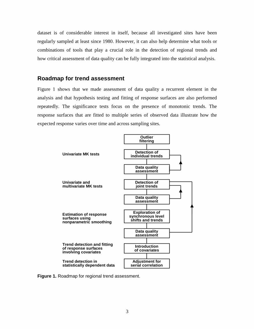
Figure 1 shows that we made assessment of data quality a recurrent element in the
analysis and that hypothesis testing and fitting of response surfaces are also performed
repeatedly. The significance tests focus on the presence of monotonic trends. The
response surfaces that are fitted to multiple series of observed data illustrate how the
expected response varies over time and across sampling sites.
Outlierfiltering
Detection ofindividual trends
Data qualityassessment
Detection ofjoint trends
Exploration ofsynchronous levelshifts and trends
Univariate MK tests
Univariate andmultivariate MK tests
Data qualityassessment
Introductionof covariates
Estimation of responsesurfaces usingnonparametric smoothing
Trend detection and fittingof response surfacesinvolving covariates
Adjustment forserial correlation
Trend detection instatistically dependent data
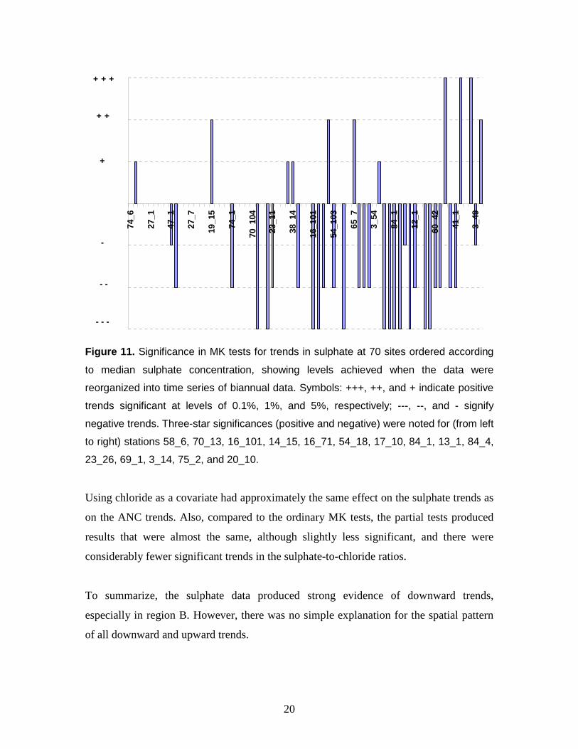
Figure 1. Roadmap for regional trend assessment.
4
The initial outlier filtering focuses on individual observations that differ strongly from the
great majority of the other observations in the same time series. Conventional criteria,
such as the number of standard deviations from the mean, can be applied to identify
observations that need to be removed or corrected prior to the trend assessment.
Thereafter, univariate MK tests and nonparametric smoothing techniques are used as
exploratory tools. More specifically, we propose the following:
(i) visual inspection of p-values for time series that are ordered with respect to
sample means or other user-defined station characteristics (see the case study);
(ii) tests for joint trends in groups of samples determined by user-defined factors
or classes;
(iii) visual inspection of response surfaces in search of synchronous trends and
level shifts in multiple data series (Wahlin and Grimvall 2008).
After each step, data quality is assessed, and erroneous data are removed or corrected.
Next, we proceed to a more formal trend analysis in which we also take into account the
impact of covariates and serial correlation. In the MK tests, covariates can be considered
by adjusting the inputs prior to the tests or by performing partial trend tests (Libiseller
and Grimvall 2002). In our response surface methodologies, the trend surface and the
impact of covariates are estimated simultaneously (Grimvall et al. 2008). Finally, we
ascertain whether the detected trends remain significant after corrections are made for
covariates and serial correlation. In the MK tests, this can be done by reorganizing the
given data into new series with longer time steps. When response surfaces are fitted to
observed data, uncertainty estimates involving block resampling can reduce the impact of
statistically dependent observations.
Significance tests for trends
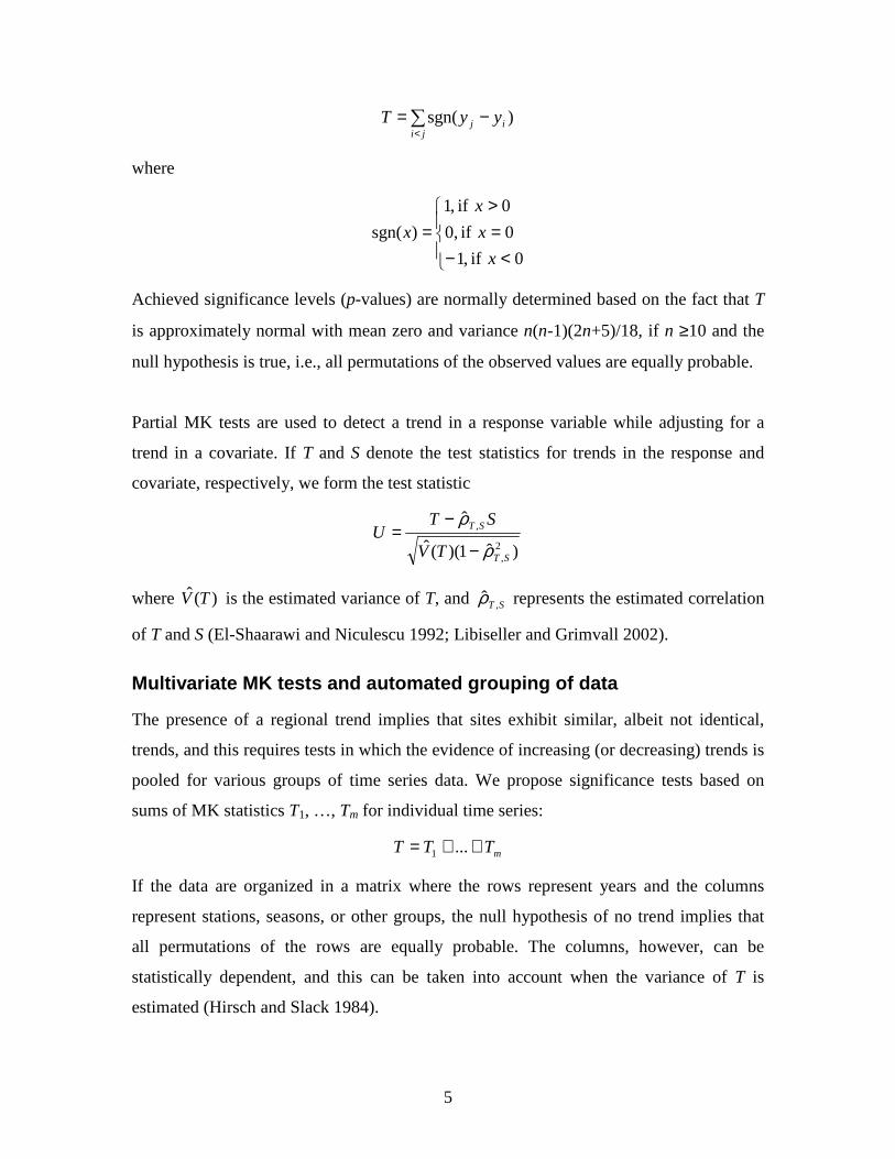
Ordinary and partial MK tests
Ordinary MK tests for monotonic trends are based on pairwise comparisons of all
observations y1, …, yn in a time series, and the test statistic is given by
5
∑<
−=ji
ij yyT )sgn(
where
<−=>
=0if,1
0if0,
0if,1
)sgn(
x
x
x
x
Achieved significance levels (p-values) are normally determined based on the fact that T
is approximately normal with mean zero and variance n(n-1)(2n+5)/18, if n ≥10 and the
null hypothesis is true, i.e., all permutations of the observed values are equally probable.
Partial MK tests are used to detect a trend in a response variable while adjusting for a
trend in a covariate. If T and S denote the test statistics for trends in the response and
covariate, respectively, we form the test statistic
)ˆ1)((ˆ
ˆ
2,
,
ST
ST
TV
STU
ρ
ρ
−
−=
where )(ˆ TV is the estimated variance of T, and ST ,ρ̂ represents the estimated correlation
of T and S (El-Shaarawi and Niculescu 1992; Libiseller and Grimvall 2002).
Multivariate MK tests and automated grouping of data
The presence of a regional trend implies that sites exhibit similar, albeit not identical,
trends, and this requires tests in which the evidence of increasing (or decreasing) trends is
pooled for various groups of time series data. We propose significance tests based on
sums of MK statistics T1, …, Tm for individual time series:
mTTT ++= ...1
If the data are organized in a matrix where the rows represent years and the columns
represent stations, seasons, or other groups, the null hypothesis of no trend implies that
all permutations of the rows are equally probable. The columns, however, can be
statistically dependent, and this can be taken into account when the variance of T is
estimated (Hirsch and Slack 1984).
6
Because groundwater data can be grouped in many different ways, for instance with
respect to sampling site, season, hydrogeological region, and other factors, it may be of
interest to undertake a large number of sum tests. If the collected data can be grouped
according to p factors, there is a total of 2p-1 sum tests in which univariate test statistics
are summed over all levels of a subset of factors. However, some of these tests can be
redundant. For example, summation over hydrogeological regions for a given station will
create a redundant sum test, because each station belongs to a single hydrogeological
region. Our procedure implies that all non-redundant sum tests are identified and
performed.
Multivariate, partial MK tests aim to assess the presence of joint trends in several groups
of data. Specifically, we assess the presence of a joint trend in the response variable that
cannot be explained by a joint trend in the covariate. The test statistic will have the same
form as in the univariate case, if we let T and S denote test statistics in sum tests for
trends in the response and covariate, respectively. Further details about partial MK tests
are given elsewhere (Libiseller and Grimvall 2002).
Handling of censored data
Observations below the limit of quantification (or detection) carry information that can
and should be exploited in trend tests when the measurement techniques have changed
over time (Helsel 2005a). We regard all observations as intervals, i.e., pairs of real
numbers. If the measured response has been quantified, the lower and upper limits of the
interval coincide, or else these limits are set to zero and the limit of quantification,
respectively.
If [ ai, bi] and [aj, bj] are two observed intervals, representing years i and j, respectively,
the sign function introduced above is modified as follows:
<−<
=otherwise,0
if,1
if,1
),,,sgn( ij
ji
jjii ab
ab
baba
7
The computation of test statistics in ordinary and partial MK statistics then proceeds as
usual. Analogously, the Theil slope of the trend is computed as the median of all ratios
ij
ab ij
−−
and ij
ba ij
−−
for i < j. In our response surface methodology, we substitute
censored observations for half the limit of quantification.
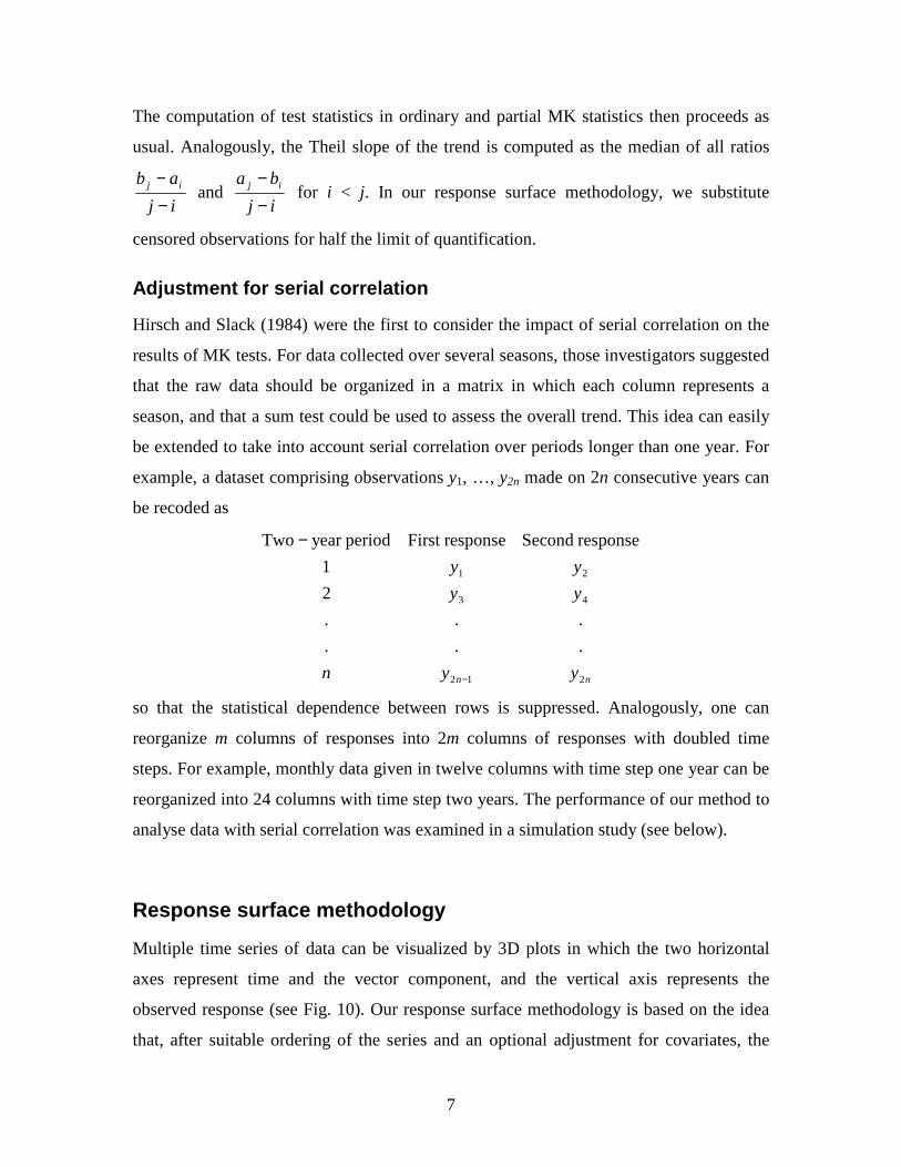
Adjustment for serial correlation
Hirsch and Slack (1984) were the first to consider the impact of serial correlation on the
results of MK tests. For data collected over several seasons, those investigators suggested
that the raw data should be organized in a matrix in which each column represents a
season, and that a sum test could be used to assess the overall trend. This idea can easily
be extended to take into account serial correlation over periods longer than one year. For
example, a dataset comprising observations y1, …, y2n made on 2n consecutive years can
be recoded as
nn yyn
yy
yy
212
43
21
...
...
2
1
response SecondresponseFirst periodyear Two
−
−
so that the statistical dependence between rows is suppressed. Analogously, one can
reorganize m columns of responses into 2m columns of responses with doubled time
steps. For example, monthly data given in twelve columns with time step one year can be
reorganized into 24 columns with time step two years. The performance of our method to
analyse data with serial correlation was examined in a simulation study (see below).
Response surface methodology
Multiple time series of data can be visualized by 3D plots in which the two horizontal
axes represent time and the vector component, and the vertical axis represents the
observed response (see Fig. 10). Our response surface methodology is based on the idea
that, after suitable ordering of the series and an optional adjustment for covariates, the
8
observed responses can be approximated by a smooth function surface. The shape of the
response (i.e., the temporal trend in the different vector components) is modelled in a
nonparametric fashion, whereas the impact of covariates is modelled parametrically
(Grimvall et al. 2008).
A roughness penalty approach is used along with cross-validation to adapt the degree of
smoothing to the data. One smoothing parameter is employed to tune the smoothing over
time, and another determines the smoothing across vector components. Explicit
roughness penalty expressions have been derived for time series representing different
seasons or several classes on a linear or circular scale. Here, we pay special attention to
data sets representing several sampling sites that are ordered with respect to the average
response at the different sites. Uncertainty bounds for the estimated response surfaces and
for trend lines representing the mean response at all sites are determined by a bootstrap
technique involving residual resampling. Further details about our response surface
methodology have been published by our research group (Grimvall et al. 2008).
Datasets
Observational data
The Geological Survey of Sweden is responsible for the national monitoring of
groundwater quality. Samples are normally taken 2–6 times a year, and they are subjected
to analysis focused on major inorganic ions, conductivity, and temperature (SGU 2008).
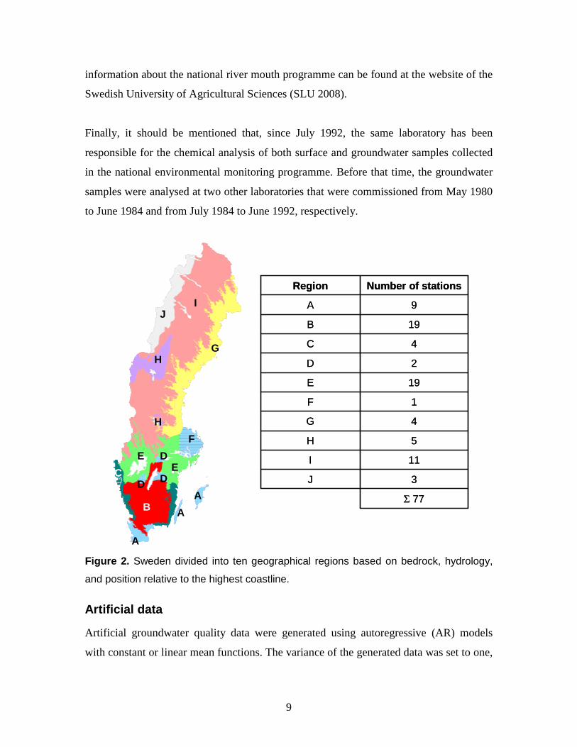
We investigated data from a total of 77 sites in ten hydrogeological regions (Fig. 2)
where sampling has been done regularly at least since 1980. In particular, we examined
the concentration of sulphate and the buffering capacity measured as alkalinity and acid-
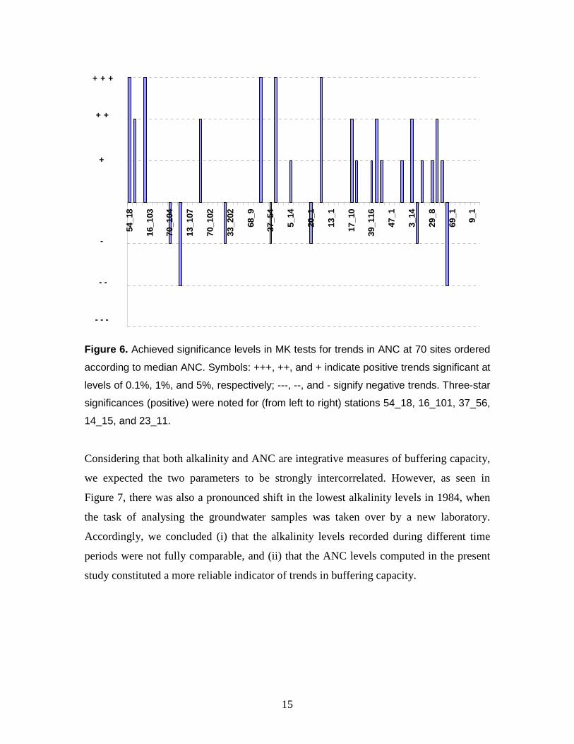
neutralizing capacity (ANC). The ANC levels were computed according to
[ ] [ ] [ ] [ ] [ ] [ ] [ ] [ ]−−−+++++ −−−++++= 3244
22 NOSOClNHKNaMgCaANC
Because the results raised questions about data quality (see below), we also examined
sulphate, alkalinity, and ANC levels in Swedish surface waters. In those analyses, we
used long time series of water quality data collected at the mouths of 37 rivers. Further
9
information about the national river mouth programme can be found at the website of the
Swedish University of Agricultural Sciences (SLU 2008).
Finally, it should be mentioned that, since July 1992, the same laboratory has been
responsible for the chemical analysis of both surface and groundwater samples collected
in the national environmental monitoring programme. Before that time, the groundwater
samples were analysed at two other laboratories that were commissioned from May 1980
to June 1984 and from July 1984 to June 1992, respectively.
Σ 77
3J
11I
5H
4G
1F
19E
2D
4C
19B
9A
Number of stationsRegion
Σ 77
3J
11I
5H
4G
1F
19E
2D
4C
19B
9A
Number of stationsRegion
JI
GH
H
F
EDE
C
B A
AD D
A
Figure 2. Sweden divided into ten geographical regions based on bedrock, hydrology,
and position relative to the highest coastline.
Artificial data
Artificial groundwater quality data were generated using autoregressive (AR) models
with constant or linear mean functions. The variance of the generated data was set to one,
10
whereas the 1-step correlation was varied from 0 to 0.4 and the slope from 0 to 0.2. The
sample size was varied from 20 to 40.
Software
MK tests
The MK tests described above are implemented in a VisualBasic macro called Multitest
(LiU 2008), which is run in Excel. Inputs are organized in tables in which the columns
represent observation years, the measured responses and covariates, and factors defining
region, sampling site, season, and so forth. The output of the macro comprises statistics
for the following tests:
(i) Ordinary MK tests for monotonic trends in univariate time series
(ii) MK sum tests for joint monotonic trends in multiple time series
(iii) Partial MK tests involving adjustment for a trend in a covariate
(iv) Partial MK sum tests adjusting for common trends in a covariate at the
investigated sites
In addition, it can be noted that the macro automatically handles censored observations
and enables adjustments for serial correlation over user-defined time spans. Automatic
generation of sum tests facilitates the testing for trends in groups of data or sites. The
output worksheets are designed to enable simple post-processing of test results, such as
sorting of p-values with respect to user-defined factors.
Semiparametric smoothing
Our smoothing methodology is implemented in a VisualBasic macro denoted Multitrend
(LiU 2008), which is run in Excel. Inputs are organized in tables containing one date
column, one column for the response under consideration, and one or more columns for
covariates. The type of smoothing (seasonal, linear or circular) is entered in UserForms.
Moreover, the user can choose between different options to determine smoothing
parameters and to compute uncertainty bounds by applying resampling techniques. The
output of the macro comprises trend surfaces and associated uncertainty bounds. In
addition, the macro computes a trend line with uncertainty bounds for the average
expected response of the investigated series.
11
Results
Impact of serial correlation
Adjustments of test statistics for serial correlation are performed to achieve better
agreement between actual and nominal significance levels when the underlying data are
statistically dependent. On the other hand, if data are independent, such adjustments will
inevitably reduce the power of the test. As expected, our method to reorganize the given
data into a larger number of shorter samples led to considerable trade-off between the
accuracy of the nominal significance level and the power of the test. However, our
simulations also showed that it is possible to achieve a satisfactory compromise between
desirable and undesirable effects, provided the time series formed in the reorganization
are at least 10 data points long.
Figure 3 shows that the loss of power was relatively small when a twenty-year time series
was split into two ten-year series, each with a time step of two years, whereas the loss
was more substantial when the original series was split into four five-year series, each
with a time step of four years. Further simulations (not shown) demonstrated that a forty-
year time series could be split into four ten-year series without substantial loss of power.
The actual and nominal significance levels of our test are identical if the autocorrelation
range does not exceed the time step of the new series formed by reorganizing the original
data. However, Figure 4 shows that, even if the underlying data are generated from a first
order autoregressive process with a theoretically infinite autocorrelation range, our
method substantially reduces the error in the nominal significance levels.
12
0.0
0.1
0.2
0.3
0.4
0.5
0.6
0.7
0.8
0.9
1.0
0 0.05 0.1 0.15 0.2
Trend slope
Po
wer
k = 1 k = 2 k = 4
Figure 3. Power functions of MK tests when the original 20-year data series was split
into k series with a time step of n/k. Raw data comprised independent normal random
variables with variance one and linear slope from 0 to 0.2. The nominal significance level
was 5% (one-sided).
0%
2%
4%
6%
8%
10%
12%
14%
16%
18%
0 0.1 0.2 0.3 0.4
Autocorrelation
Act
ual
sig
nif
ican
ce l
evel
k = 1 k = 2 k = 4
Figure 4. Actual significance levels of MK tests based on original and reorganized data
when the original series were generated according to AR(1) processes with ρ = 0, 0.1,
0.2, 0.3, and 0.4. The parameter k refers to the time step in the reorganized data series,
and the nominal significance level was 5% (one-sided).
13
Alkalinity and ANC trends in groundwater
A search for outliers in the reported concentrations of major cations and anions revealed
that there were obvious errors in the chemical composition of 148 of the 5,557 samples
considered in the present study, and hence those samples were omitted from the trend
analysis. Moreover, we excluded all data from seven of the 77 investigated sites, because
both the MK statistics for temporal trends and visual inspection of collected data clearly
indicated local pollution, presumably from road salt.
When ordinary univariate MK tests were again employed to examine the presence of
trends in alkalinity levels, and the investigated sites were ordered according to median
alkalinity, the striking pattern evident in Figure 5 emerged. As can be seen in the figure,
we found significant downward trends at sites with low alkalinity and upward trends at
sites with high alkalinity. The downward trends were not anticipated, because the acid
deposition in Sweden has decreased considerably over the past two decades, and low
alkalinity groundwaters are found primarily in aquifers with relatively short residence
times. In addition, the downward trends in groundwater were contradicted by upward
trends in river water. When we performed MK tests for trends in alkalinity in 37 Swedish
sampling sites, as expected, we observed the strongest upward trends in low alkalinity
rivers located in regions that were previously exposed to considerable sulphur deposition.
14
54_1
8
41_1
70_1
3
89_6
50_1
4
5_13
37_5
4
33_1
04
84_4
89_7
38_1
4
75_2
20_1
0
39_7
23_2
3
3_54
41_5
+ + +
+ +
+
- - -
- -
-
Figure 5. Achieved significance levels in MK tests for trends in alkalinity at 70 sites
ordered according to median alkalinity. Symbols: +++, ++, and + indicate positive trends
significant at levels of 0.1%, 1%, and 5%, respectively; ---, --, and - signify negative
trends. The station labels refer to the national Swedish groundwater monitoring
programme. Three-star significances (positive and negative) were noted for (from left to
right) stations 58_4, 13_107, 33_202, 19_15, 20_1, 75_2, 70_14, 3_14, 3_53, 29_8,
3_49, and 9_1.
To further elucidate the existence of acidification trends in groundwater, we also
examined time series of ANC levels. Figure 6 shows the achieved significance levels. In
contrast to the results for alkalinity, the most significant upward trends in ANC were
discerned for groundwaters with low to medium buffering capacity. In addition, we noted
that there was generally good agreement between the ANC trends in groundwater and
river water (not shown).
15
54_1
8
16_1
03
70_1
04
13_1
07
70_1
02
33_2
02
68_9
37_5
4
5_14
20_1
13_1
17_1
0
39_1
16
47_1
3_14
29_8
69_1 9_1
+ + +
+ +
+
- - -
- -
-
Figure 6. Achieved significance levels in MK tests for trends in ANC at 70 sites ordered
according to median ANC. Symbols: +++, ++, and + indicate positive trends significant at
levels of 0.1%, 1%, and 5%, respectively; ---, --, and - signify negative trends. Three-star
significances (positive) were noted for (from left to right) stations 54_18, 16_101, 37_56,
14_15, and 23_11.
Considering that both alkalinity and ANC are integrative measures of buffering capacity,
we expected the two parameters to be strongly intercorrelated. However, as seen in
Figure 7, there was also a pronounced shift in the lowest alkalinity levels in 1984, when
the task of analysing the groundwater samples was taken over by a new laboratory.
Accordingly, we concluded (i) that the alkalinity levels recorded during different time
periods were not fully comparable, and (ii) that the ANC levels computed in the present
study constituted a more reliable indicator of trends in buffering capacity.
16
0
0.05
0.1
0.15
0.2
0.25
0.3
0.35
0.4
0.45
0.5
-0.25 -0.15 -0.05 0.05 0.15 0.25 0.35 0.45
ANC (meq/l)
Alk
alin
ity
(meq
/l)
1992-2007 1985-1991 1980-1984
Figure 7. Alkalinity levels in groundwater plotted against acid neutralizing capacity. The
three time periods represent data from the three different laboratories that were
commissioned to perform the monitoring.
Further analysis of the ANC data revealed pronounced serial correlation for many of the
investigated time series. Therefore, we also computed the achieved significance levels in
MK tests where we suppressed the effect of serial correlation by reorganizing the data
into biannual time series. However, as can be seen in Figure 8, there was still clear
evidence of upward trends in ANC. The strongest trends prevailed in waters with low to
medium alkalinity in southern Sweden, whereas there were weak or nonexistent trends in
northern Sweden.
Chloride is sometimes used as an indicator of soil water movement, because, correctly or
not (Bastviken et al. 2007; Schlesinger 1997), it is considered to be inert in soil.
Accordingly, we undertook partial MK tests of ANC levels, using chloride as a covariate.
Furthermore, we computed ANC-to-chloride ratios that we tested for trends. Compared to
the ordinary MK tests, the partial tests produced results that were almost the same, albeit
17
slightly less significant. There were considerably fewer significant trends in the ANC-to-
chloride ratios, because the formation of such ratios increased the coefficient of variation
of the data that were analysed for trends.
In summary, our trend assessment provided strong evidence of upward ANC trends in the
areas where acid deposition has decreased over the past decades. However, there was
considerable variation between the sampling sites.
54_1
8
16_1
03
70_1
04
13_1
07
70_1
02
33_2
02
68_9
37_5
4
5_14
20_1
13_1
17_1
0
39_1
16
47_1
3_14
29_8
69_1 9_1
+ + +
+ +
+
- - -
- -
-
Figure 8. Significance in MK tests for trends in ANC at 70 sites ordered according to
median ANC, showing levels achieved when the data were reorganized into time series
of biannual data. Symbols: +++, ++, and + indicate positive trends significant at levels of
0.1%, 1%, and 5%, respectively; ---, --, and - signify negative trends. Three-star
significance (positive) was noted for station 16_101.
Sulphate trends
Figure 9 illustrates the results of MK tests for sulphate trends. Apparently there were
many downward trends but only a few upward trends. Closer examination of the test
results revealed that there were several statistically significant downward trends in
18
southern Sweden, particularly in hydrogeological region B (see Fig. 2), whereas the
trends in Northern Sweden were weak or nonexistent. The trends detected in region B
were expected, because (i) the sulphur deposition in that part of Sweden has decreased
significantly over the past decades, and (ii) shallow moraines on a primary bedrock
enable rapid response to changes in deposition. Furthermore, the results of our analysis
were concordant with the pronounced downward trends that were revealed when we
analysed river water data from the same region.
74_6
27_1
47_1
27_7
19_1
5
74_1
70_1
04
23_1
1
38_1
4
16_1
01
54_1
03
65_7
3_54
84_1
12_1
60_4
2
41_1
3_49
+ + +
+
- - -
- -
-
Figure 9. Achieved significance levels in MK tests for sulphate trends at 70 sites ordered
according to median sulphate concentration. Symbols: +++, ++, and + indicate positive
trends significant at levels of 0.1%, 1%, and 5%, respectively; ---, --, and - signify
negative trends. Three-star significances (positive and negative) were noted for (from left
to right) stations 23_23, 19_15, 74_1, 58_6, 70_13, 23_11, 33_104, 16_28, 16_101,
14_15, 5_14, 54_103, 16_71, 65_7, 70_14, 16_102, 54_18, 17_10, 84_1, 13_1, 84_4,
12_1, 23_26, 69_1, 60_42, 69_10, 3_14, 21_9, 41_1, 75_2, 20_10, and 41_5.
Further examination of the sulphate levels in region B showed that the average
concentration in that area decreased at about the same rate over the entire study period.
19
However, there was substantial variation between sites, which is illustrated by the trend
surface in Figure 10.
1980
1983
1986
1989
1992
1995
1998
2001
2004
2007
74_616_101
5_1416_103
17_100
0.05
0.1
0.15
0.2
0.25
0.3
0.35
0.4
0.45S
O4
con
c. (
meq
/l)
Figure 10. Trend surface fitted to observed sulphate concentrations at the 19
investigated stations in hydrogeological region B.
Inasmuch as repeated assessments of data quality constitute an important part of our
roadmap, we also searched for inexplicable level shifts in the reported sulphate
concentrations. We noted that the major changes in sulphate levels seemed to be caused
by natural dilution processes, because they normally coincided temporally with natural
fluctuations in conductivity and other major ions. However, inspection of raw data and
deviations from the fitted response surfaces also indicated a substantial serial correlation
in the analysed time series. Consequently, we repeated the MK tests on data that had been
reorganized in series with longer time steps. Figure 11 presents the results obtained when
the impact of serial correlation for up to two years was suppressed. As can be seen, many
significant downward trends remained.
20
74_6
27_1
47_1
27_7
19_1
5
74_1
70_1
04
23_1
1
38_1
4
16_1
01
54_1
03
65_7
3_54
84_1
12_1
60_4
2
41_1
3_49
+ + +
+ +
+
- - -
- -
-
Figure 11. Significance in MK tests for trends in sulphate at 70 sites ordered according
to median sulphate concentration, showing levels achieved when the data were
reorganized into time series of biannual data. Symbols: +++, ++, and + indicate positive
trends significant at levels of 0.1%, 1%, and 5%, respectively; ---, --, and - signify
negative trends. Three-star significances (positive and negative) were noted for (from left
to right) stations 58_6, 70_13, 16_101, 14_15, 16_71, 54_18, 17_10, 84_1, 13_1, 84_4,
23_26, 69_1, 3_14, 75_2, and 20_10.
Using chloride as a covariate had approximately the same effect on the sulphate trends as
on the ANC trends. Also, compared to the ordinary MK tests, the partial tests produced
results that were almost the same, although slightly less significant, and there were
considerably fewer significant trends in the sulphate-to-chloride ratios.
To summarize, the sulphate data produced strong evidence of downward trends,
especially in region B. However, there was no simple explanation for the spatial pattern
of all downward and upward trends.
21
Discussion and conclusions
Groundwater monitoring programmes aim to detect human impacts that can be rather
small compared to the weather-driven fluctuations and random measurement errors that
influence individual observations. Accomplishment of that objective requires statistical
methods that strongly suppress purely random variation, and the standard procedure is to
pool data from several sampling sites and focus the statistical analysis on overall patterns
in large amounts of data. We have now gone one step further by emphasizing the need for
a sequence of coordinated statistical analyses that are integrated into a roadmap for
simultaneous assessment of trends and data quality. The proposed collection of MK tests
proved to be an efficient tool to detect relatively small upward or downward shifts in
substantial amounts of data, and our response surface methodology provided valuable
information about the timing of water quality changes at different sites.
Our study also showed that assessment of data quality should be repeated at all stages of
the statistical data analysis. In particular, we found that examination of patterns in
achieved significance levels of MK tests can effectively reveal spurious trends caused by
long-lasting measurement errors. Our response surface methodology forms a natural
complement to the MK tests by providing information about synchronous level shifts that
may indicate changes in sampling and laboratory practices. However, it is important to
note that none of the mentioned methods will separate long-lasting systematic
measurement errors from actual trends. Therefore, trend analysis is also a matter of
judging the plausibility of the extracted spatio-temporal patterns in the state of the
environment.
The role of judgments can be illustrated with our analysis of alkalinity and ANC data.
The MK tests for trends in alkalinity played a key role, because they revealed an
unexpected pattern in the achieved significance levels (p-values). Furthermore, simple
scatter plots showed that there was a shift in the alkalinity-to-ANC ratios of acidic
samples in 1984 when a different laboratory was engaged to analyse water samples.
However, we also judged that the computed ANC trends were much more plausible than
the alkalinity trends. In our recent study of trends in Swedish surface waters (Wahlin and
22
Grimvall 2008), it was our response surface methodologies that played the most decisive
role. The fitted surfaces revealed unexpectedly synchronous trends and level shifts in
samples that had been taken at geographically separated sites but were analysed in the
same laboratory. This observation triggered investigations that eventually led to the
judgment that many time series of total nitrogen and phosphorous levels were more
extensively influenced by changes in the laboratory than by actual changes in the
environment. Furthermore, it is noteworthy that in both the groundwater and surface
water studies the ordering of stations with respect to median concentrations helped reveal
remarkable spatio-temporal patterns in the analysed data.
Standardization or normalization of environmental quality data is sometimes done to
clarify temporal trends in the human impact on the environment. For example, river water
quality can be normalized with respect to water discharge, and air quality with regard to
various meteorological covariates (Hussian et al. 2004; Libiseller et al. 2003). Here, we
compared the results obtained using ordinary MK tests and partial MK tests with chloride
as covariate. In addition, we formed ANC-to-chloride and sulphate-to-chloride ratios that
were subsequently analysed by ordinary MK tests. As pointed out, the use of partial tests
and especially the calculation of ratios, resulted in fewer significant test results. This was
expected in the present study, because (i) the peaks and troughs in ANC, sulphate, and
chloride were not particularly synchronous, and (ii) the trends in chloride were generally
weak at the investigated sites. In other studies, partial MK tests may provide more
important information.
Serial correlation is another issue that needs to be considered in any assessment of
temporal trends in environmental data. It is well known that even a moderately large
autocorrelation can make the actual significance level considerably higher than the
nominal level. A few years ago, Yue and Wang (2004) conducted a comprehensive
review of the methods that have been used to adjust achieved significance levels with
respect to serial correlation. In short, those authors concluded that all existing procedures
have substantial shortcomings and that adjustment factors should be derived from
detrended data series. We found that a simple generalization of the idea behind Hirsch
23
and Slack’s trend test for seasonal data is a viable alternative to the techniques currently
in use. In particular, our method has the advantage that it can be applied to any of the MK
tests proposed in the present article. Furthermore, it is not restricted to specific parametric
forms of trend functions and autocorrelation functions. The performance of our method
was satisfactory for autocorrelation ranges up to one tenth of the total length of the
current study period.
The handling of censored data is yet another topic that needs to be addressed. We used
the concepts reported by Helsel (2005a and b) and applied them to ordinary and partial
MK tests, and to estimation of Theil slopes (Sen 1968; Theil 1950).
In conclusion, we have presented a set of statistical methods that address the most
common problems encountered in trend analysis of groundwater quality, and we have
integrated those techniques into a roadmap for such investigations. In addition, we have
developed a software package that greatly facilitates joint analysis of multiple time series
of data. Our case study revealed both actual trends and artificial level shifts that would
have been difficult to detect if the time series had been analysed one by one.
Acknowledgements
The authors are grateful for financial support from the Geological Survey of Sweden and
the Swedish Environmental Protection Agency.
References Bastviken D., Thomsen F., Svensson T., Karlsson S., Sandén P., Shaw G., Matucha M.
and Öberg G. (2007). Chloride retention in forest soil by microbial uptake and by natural
chlorination of organic matter. Geochimica et Cosmochimica Acta, 71, 3182-3192.
Brockwell P.J. and Davis R.A. (1996). Introduction to time series and forecasting.
Springer: New York.
24
Cameron K. and Hunter P. (2002). Using spatial models and kriging techniques to
optimize long-term ground-water monitoring networks: a case study. Environmetrics, 13,
629-656.
El-Shaarawi A.H. and Niculescu S. (1992). On Kendall’s tau as a test for trend in time
series data. Environmetrics, 3, 385-411.
Finkenstadt B., Held L. and Isham V. (2006). Statistical methods for spatio-temporal
systems. Chapman & Hall/CRC: London.
Fuentes M. (2002). Spectral methods for nonstationary spatial processes. Biometrika, 89,
197-210.
Grath J., Ward R. and Quevauviller P. (eds) (2007). Common implementation strategy
for the water framework directive. Guidance on groundwater monitoring. Office for
Official Publications of the European Communities: Luxembourg.
Griliches Z. and Intriligator M.D. (eds) (1983). Handbook of econometrics. Elsevier:
Amsterdam. http://www.sciencedirect.com/science/handbooks/15734412. Accessed 28
June 2008.
Grimvall A., Wahlin K., Hussian M. and Libiseller C. (2008). Semiparametric smoothers
for trend assessment of multiple time series of environmental quality data. Submitted to
Environmetrics.
Helsel D.R. (2005a). More than obvious: better methods for interpreting nondetect data.
Environmental Science and Technology, October 15, 2005.
Helsel D.R. (2005b). Insider censoring: distortion of data with nondetects. Human and
Ecological Risk Assessment, 11, 1127-1137.
25
Hirsch R.M. and Slack J.R. (1984). A non-parametric trend test for seasonal data with
serial dependence. Water Resources Research, 20, 727–732.
Hussian M., Grimvall A. and Petersen W. (2004). Estimation of the human impact on
nutrient loads carried by the Elbe River. Environmental Monitoring and Assessment, 96,
15-33.
Libiseller C. and Grimvall A. (2002). Performance of partial Mann-Kendall test for trend
detection in the presence of covariates. Environmetrics, 13, 71-84.
Libiseller C., Grimvall A., Waldén J. and Saari H. (2003). Meteorological normalisation
and non-parametric smoothing for quality assessment and trend analysis of tropospheric
ozone data. Environmental Monitoring and Assessment, 100, 33-52.
LiU (Linköping University) (2008). http://www.ida.liu.se/divisions/stat/research/.
Accessed 2008-08-20.
Loftis J.C., Taylor C.H. and Chapman P.L. (1991). Multivariate tests for trend in water
quality. Water Resources Bulletin, 24, 505-512.
Scharf L. (1990). Statistical signal processing. Prentice Hall: New Jersey.
Schlesinger W. (1997). Biogeochemistry. An Analysis of Global Change. Academic
Press: San Diego.
Sen P.K. (1968). Estimates of the regression coefficient based on Kendall's tau. Journal
of the American Statistical Association, 63, 1379-1389.
SGU (Geological Survey of Sweden) (2008).
http://www.sgu.se/sgu/sv/samhalle/miljo/miljoovervakning/overvakning-
grundvatten.html. Accessed 2008-08-20.
26
SLU (Swedish University of Agricultural Sciences) (2008).
http://www.ma.slu.se. Accessed 2008-08-20.
Theil H. (1950). A rank-invariant method of linear and polynomial regression analysis, I,
II, and III. Nederlandsche Akad. van Wetenschappen Proc., 58, 386-392, 521-525 and
1397-1412.
Thompson M.L., Reynolds J., Cox L.H., Guttorp P. and Sampson P.D. (2001). A review
of statistical methods for the meteorological adjustment of ozone. Atmospheric
Environment, 35, 617-630.
Wahlin K. and Grimvall A. (2008). Uncertainty in water quality data and its implications
for trend detection: lessons from Swedish environmental data. Environmental Science
and Policy, 11, 115-124.
Yue S. and Wang C.Y. (2004). The Mann-Kendall test modified by effective sample size
to detect trend in serially correlated hydrological series. Water Resources Management,
18, 201-218.