Robotica //rpk.lcsr.jhu.edu/wp-content/uploads/2016/08/Kim16_Inverse... · Robotica Additional...

Roboticahttp://journals.cambridge.org/ROB

Additional services for Robotica:

Email alerts: Click hereSubscriptions: Click hereCommercial reprints: Click hereTerms of use : Click here

Inverse kinematic solutions of 6-D.O.F. biopolymer segments

Jin Seob Kim and Gregory S. Chirikjian

Robotica / Volume 34 / Issue 08 / August 2016, pp 1734 - 1753DOI: 10.1017/S0263574716000138, Published online: 13 April 2016

Link to this article: http://journals.cambridge.org/abstract_S0263574716000138

How to cite this article:Jin Seob Kim and Gregory S. Chirikjian (2016). Inverse kinematic solutions of 6-D.O.F. biopolymer segments. Robotica, 34,pp 1734-1753 doi:10.1017/S0263574716000138

Request Permissions : Click here

Downloaded from http://journals.cambridge.org/ROB, IP address: 128.220.160.131 on 15 Aug 2016

http://journals.cambridge.org Downloaded: 15 Aug 2016 IP address: 128.220.160.131

Robotica (2016) volume 34, pp. 1734–1753. © Cambridge University Press 2016doi:10.1017/S0263574716000138

Inverse kinematic solutions of 6-D.O.F. biopolymersegmentsJin Seob Kim and Gregory S. Chirikjian∗

Department of Mechanical Engineering, Johns Hopkins UniversityBaltimore, MD 21218, USA. E-mail: [email protected]

(Accepted February 24, 2016. First published online: April 13, 2016)

SUMMARYWe present two methods to find all the possible conformations of short six degree-of-freedomsegments of biopolymers which satisfy end constraints in position and orientation. One of ourmethods is motivated by inverse kinematic solution techniques which have been developed for“general” 6R serial robotic manipulators. However, conventional robot kinematics methods are notdirectly applicable to the geometry of polymers, which can be treated as a degenerate case whereall the “link lengths” are zero. Here, we propose a method which extends the elimination methodof Kohli and Osvatic. This method can be applied directly to the geometry of biopolymers. We alsopropose a heuristic method based on a Lie-group-theoretic description. In this method, we utilizeinverse iterations of the Jacobian matrix to obtain all conformations which satisfy end constraints.This can be easily implemented for both the general 6R manipulator and polymers. Although theextended elimination method is computationally faster than the Jacobian method, in cases wheresome of the joint angles are 180◦ (i.e., where the elimination method fails), we combine these twomethods effectively to obtain the full set of inverse kinematic solutions. We demonstrate our approachwith several numerical examples.

KEYWORDS: Biopolymer structure; 6R manipulator; Inverse kinematics; Eigenvalue problem; Lie-group-theoretic method; Jacobian matrix.

1. IntroductionDuring the past decades, the conformational analysis of polymers has been of great interest in the areaof polymer science and biophysics. Several methods for this purpose have been utilized for simulatingthe motions of a polymer and sampling the space of preferred conformations. One of those methodsincludes Monte Carlo simulation. Regarding this famous statistical method, researchers have beeninterested in “local moves” for Monte Carlo sampling, which generates multiple conformations ofa short polymer segment without causing any great change in global geometry.1–3 This is especiallyuseful when one is interested in the Monte Carlo sampling of polymer structures with fixed ends.4

For example, suppose that we have a long chain-like biopolymer molecule. When we change onetorsional angle in the middle of a polymer chain by a small amount, then the position and orientationof the last molecule of a chain can vary a lot. In this case, we need so-called “concerted rotation” or“local moves”. In order to use this method, one needs to solve the inverse kinematics of a polymerwith given end constraints. This can be solved efficiently when methods of robotic kinematics areapplied. The simplified backbone geometry of a polymer is shown in Fig. 1. Looking at this figure,we can see that it is very similar to the geometry of the general robotic manipulator except when allof the adjacent axes of rotation intersect each other. In this paper, we review methods for solvingthe inverse kinematics problem for general 6R manipulators and propose modifications to deal withinverse kinematic problems for polymer geometries where the robotics techniques break down. Wealso present a method based on a Lie-group-theoretic description that can be applied and implementedeasily compared with other methods to both the geometries of polymers and robot manipulators. Using

* Corresponding author. E-mail: [email protected]

http://journals.cambridge.org


Inverse kinematic solutions 1735

z

yx

z

θi α i

Li

Fig. 1 The schematic conformation of a polymer used in this paper.

a combination of the proposed two methods enables us to obtain all true inverse kinematic solutionsof 6-D.O.F. biopolymer structures even when there are kinematically degenerate cases such as whensome of the joint angles are equal to 180◦.

1.1. Literature reviewPast theoretical works on “local movements” in polymer chains include the work of Go andScheraga.5–7 Based on their pioneering work, Dodd at al. analyzed this motion with the concept ofthe “concerted rotation” method.8 They were dealing with seven adjacent dihedral angles in polymerstructures, one of which was the driving angle to generate the “concerted rotation”. In this approach,one numerically solves non-linear algebraic equations in order to obtain the inverse kinematicsolutions. Several researchers have applied this concerted rotation method to protein structures.2, 3, 9–13

Another approach was introduced by Wedemeyer and Scheraga,14 where the polynomial equationswith respect to dihedral angles were derived through spherical geometric relations. On the other hand,some researchers in the chemical physics community have adopted Lee and Liang’s method15, 16 toformulate the eigenvalue/eigenvector techniques of Manocha and Canny17 for polypeptide kinematicsincluding the special case which contains proline.18

Many researchers have studied the inverse kinematics of “general” 6R serial manipulators thatwork in all cases except for special combinations of link parameters and joint angles.15, 16, 19–24

From these works, the maximum number of inverse kinematic solutions is shown to be 16. Amongthese, the formulation of Raghavan and Roth has been the basis of several other methods developedthereafter. In Raghavan and Roth’s work, they constructed 14 equations from the basic homogeneoustransformation equations and used the characteristic equation of a 12 × 12 matrix to get the inversekinematic solutions.23, 24 To avoid lengthy calculations of the determinant of a 12 × 12 matrix andsolving a 16th-order polynomial equation, Manocha and Canny formulated an eigenvalue problemto find the inverse kinematic solutions.17 Based on Raghavan and Roth’s work, they used matrixpolynomials to get an augmented matrix whose size is 24 × 24. Then, the inverse kinematics problemcan be reduced to an eigenvalue problem, which means it can be solved accurately and efficiently.Based on their formulation, Manocha et al. developed an extended version of Manocha–Cannyformulation which can be applied to polymer structure.25 In their work, the minimum size of a matrixfor the eigenvalue problem is 32 × 32. Meanwhile, Kohli and Osvatic developed another methodwhich computes inverse kinematics solutions as an eigenvalue problem by constructing a 16 × 16matrix, which is linear in one suppressed variable.26 Ghazvini also devised a method similar to that ofKohli and Osvatic.27 His formulation also contained only one suppressed variable in the final form ofmatrix equation. However, in his formulation, matrices bigger than 16 × 16 were generated. Nielsenand Roth summarized the state-of-the-art techniques for solving the inverse kinematics of 6 degree-of-freedom serial manipulators and direct kinematics of parallel manipulators.28 Their paper discussespower products and dialytic elimination which are based on the work of Raghavan and Roth.23, 24

Husty et al. proposed a method based on classical multi-dimensional differential geometry to solvea univariate polynomial equation for a general 6R robot manipulator.29 A recent work develops amethod to find intersection curves of four bivariate polynomial equations that can be derived basedon Raghavan and Roth’s formulation.30

1.2. Motivation and organizationAmong the works discussed above, Kohli and Osvatic’s work seems to be the least well known, butthis work is interesting because it requires solving the smallest eigenvalue problem. It is similar to



1736 Inverse kinematic solutions

that of Manocha and Canny in that they both used eigenvalue problems to get solutions. However,Kohli and Osvatic construct a 16×16 matrix in their work, which is smaller than that in Manocha andCanny’s work and generates exactly the same number of eigenpairs as the maximum possible numberof inverse kinematic solutions. Furthermore, the matrix equations appearing in their paper has onlyone suppressed variable. For these reasons, we adopt the method in Kohli and Osvatic’s work. In thesubsequent sections, we review that method and introduce our extension. We also explain why thedirect application of techniques from manipulator inverse kinematics using eigenvalue/eigenvectorformulation, such as work of Kohli and Osvatic26 and that of Manocha and Canny,17 does not work forthe geometry of polymers. After that, we give a brief introduction to the Lie-group-theoretic notation,and explain so-called Jacobian method. Numerical examples follow thereafter.

2. Inverse Kinematics as an Eigenvalue/Eigenvector Problem

2.1. The method of Kohli and OsvaticAs mentioned in Section 1, we adopt Kohli and Osvatic’s method to find the general inverse kinematicsolutions. We give a brief explanation of their method below. For a more detailed explanation, seethe work of Kohli and Osvatic.26 Since Raghavan and Roth23, 24 built the fundamental formulationfor both the work of Manocha and Canny17 and that of Kohli and Osvatic,26 we start the review withtheir formulation.

The basic matrix form of the equation which Raghavan and Roth used is

H1H2H3H4H5H6 = Hee, (1)

where Hi , (i = 1, . . . , 6) is a homogeneous transformation matrix according to the Denavit–Hartenberg (DH) representation, and can be expressed as31

Hi =

⎛⎜⎝

cos(θi) − sin(θi) cos(αi) sin(θi) sin(αi) ai cos(θi)sin(θi) cos(θi) cos(αi) − cos(θi) sin(αi) ai sin(θi)

0 sin(αi) cos(αi) Li

0 0 0 1

⎞⎟⎠ ,

where θi is a joint angle at joint i, αi is a twist angle, ai is a link length, and Li is a offset atjoint i. All these four symbols are called DH parameters. Looking at Fig. 1, since we choose thelocal z axis coincident with the backbone of a polymer, one can see that polymer structures have thecharacteristics as ai = 0. Hee is the position and orientation of the end effector. To avoid the analyticalcomplexity of Eq. (1), they follow Tsai and Morgan20 and rewrite the basic matrix equation in thenew form:

H3H4H5 = H−12 H−1

1 HeeH−16 . (2)

By extracting the third and fourth columns in both sides (from first to third elements of each columnexcluding the last element which is 1), denoted as l and p respectively, six basic equations can beconstructed. To be more specific, let the third and the fourth columns in the left-hand side be lL

and pL, respectively. Those in the right-hand side are denoted as lR and pR , respectively. Then, theequations are obtained by setting lL = lR and pL = pR . Since each equation has three components,the total number of equations becomes six. This description of the equations will be used throughoutthe paper. Furthermore, eight more independent scalar equations are obtained in the same way byconsidering the following terms:

p · p, p · l, p × l, ( p · p) l − (2 p · l) p

and combining these eight equations with basic six equations lead to 14 equations as in Raghavanand Roth’s work.23, 24 Note that due to trigonometric rules these relations all have the same “powerproducts” as p and l , i.e., all of these terms are linear combinations of elements in the set {s1s2, s1c2,c1s2, c1c2, s1, c1, s2, c2, s4s5, s4c5, c4s5, c4c5, s4, c4, s5, c5, 1}, where si = sin(θi) and ci = cos(θi),(i = 1, 2, 4, 5).




At this point, Kohli and Osvatic used the two trigonometric relations t3 sin(θ3) + cos(θ3) = 1 andsin(θ3) − t3 cos(θ3) = t3, where t3 = tan(θ3/2), to get eight new equations. Finally, Kohli and Osvaticarranged the 14 equations as follows. First, one has six equations which are independent of θ3 as

pz, lz, ( p × l)z, ( p · p)lz − (2 p · l)pz, p · l, p · p, (3)

and eight equations which are linearly dependent of t3 as

lx + t3ly, ly − t3lx, px + t3py, py − t3px,

( p × l)x + t3( p × l)y, ( p × l)y − t3( p × l)x,

( p · p)lx − (2 p · l)px + t3[( p · p)ly − (2 p · l)py],

( p · p)ly − (2 p · l)py − t3[( p · p)lx − (2 p · l)px],

(4)

totalling 14 equations. Here, lx , ly and lz, respectively denote the first, the second, and the thirdcomponents of l . The same notations are applied to p.

With the first six equations in Eq. (3), which are independent of θ3, one constructs the followingmatrix equation:

L1 y1 = R1 y2, (5)

where L1 and R1 are 6 × 11 and 6 × 6 matrices, respectively. Here, vectors in the left-hand andright-hand side are defined as

y1 = [c4c5 c4s5 s4c5 s4s5 c4 s4 c5 s5 c2 s2 1

]T

and

y2 = [c1c2 c1s2 s1c2 s1s2 c1 s1

]T.

The remaining eight equations in Eq. (4), which are linearly dependent of t3, can be arranged into thefollowing matrix form:

L2 y1 = R2 y2, (6)

where L2 and R2 are 8 × 11 and 8 × 6 matrices as functions of t3, respectively. y1 and y2 are thesame as in Eq. (5). Kohli and Osvatic combine Eqs. (5) and (6) to generate one matrix equation as

L3 y3 = 0, (7)

where

L3 = L2 − R2R−11 L1

is an 8 × 11 matrix, and y3 is defined as

y3 = [ c4c5 c4s5 s4c5 s4s5 c4 s4 c5 s5 c2 s2 1 ]T .

As the next step, they make the substitution using the trigonometric relations:

s4 = 2t4

1 + t24

c4 = 1 − t24

1 + t24

s5 = 2t5

1 + t25

c5 = 1 − t25

1 + t25

,

where t4 = tan(θ4/2) and t5 = tan(θ5/2). Hence, the eight equations can be rearranged, aftermultiplied by the denominator (1 + t2

4 )(1 + t25 ), as

L4 y4 = 0, (8)




where L4 is an 8 × 11 matrix, and y4 is defined as

y4 = [t24 t2

5 t24 t5 t4t

25 t2

4 t5 t4t5 t24 t4 t2

5 J K 1]T

,

where J = cos(θ2)(1 + t24 )(1 + t2

5 ), and K = sin(θ2)(1 + t24 )(1 + t2

5 ). They also multiply the eightequations by t4 to get another eight equations, which, together with the previous eight equations inEq. (8), gives a set of 16 equations, and the set of 16 equations can be arranged into the followingmatrix form:

L5v = 0, (9)

where the column vector v is defined as

v = [t34 t2

5 t34 t5 t3

4 t24 t2

5 t24 t5 t2

4 t4t25 t4t5 t4J t4K t4 t2

5 t5 J K 1]T

.

Here, J and K are the same as in the definition of y4. L5 is a 16×16 matrix, which is expressed asAt3 + B, where t3 = tan(θ3/2) and A and B are 16×16 matrices which can be treated as constantmatrices. Consequently, the inverse kinematic solutions of a general 6R robot manipulator can beobtained by solving the generalized eigenvalue problem

Bv = −t3Av, (10)

where v is the 16×1 vector which appears in the left-hand side of Eq. (9), and t3 is the correspondingeigenvalue.

After finding eigenvalues and corresponding eigenvectors of (10), one can find all the joint variablessequentially. For one value of t3, one can determine θ3, and one can also determine θ2, θ4 and θ5 byfinding J , K , t4 and t5, which can be calculated by normalizing the corresponding eigenvector, where“normalize” means that the last element of the eigenvector should be 1. After that, substitution of θ2,θ3, θ4 and θ5 into Eqs. (5) or (6) gives θ1, and finally by Eqs. (1) or (2), we can determine θ6.

3. Inverse Kinematics for Biopolymer StructuresThe key to this solution method is to solve the eigenvalue problem in Eq. (10). If A is non-singular,then the problem reduces to the conventional eigenvalue problem as

−A−1Bv = t3v. (11)

In the case when A is singular, we still have the possibility to get the correct eigenvalues andeigenvectors by using a generalized eigenvalue algorithm which deals with systems of the form:

Bv = t3(−A)v. (12)

However, if the system (B + t3A)v = 0 is a singular pencil (meaning that det(B + t3A) = 0 for allvalues of t3), then solution techniques for the generalized eigenvalue problem such as the generalizedSchur decomposition or QZ algorithm32 do not give the correct answer.33 The failure of inversekinematics methods for the case of singular pencils has also been mentioned in the paper of Manochaand Canny.17

Unfortunately, a polymer structure such as a polypeptide chain or polypropylene possesses theabove property due to the fact that all the link lengths of the structure are zero. In this case, anothermethod is necessary because the algorithms of Raghavan and Roth and Manocha and Canny fail toyield solutions. Note that there are other possible methods to solve the problem in this situation.21, 29

However, we explore the eigenvalue/eigenvector formulation which we think has potential to be thefastest method. One can utilize the extended Manocha–Canny method,25 in which the minimum sizeof the matrix for the eigenvalue problem is 32 × 32. In the subsequent section, we present the extendedelimination method, which forms a smaller, and therefore more efficient, eigenvalue problem.




3.1. Implementation of the extended elimination methodIf we apply Kohli and Osvatic’s method to biopolymer structures, the rank of each resulting matrix,A and B in Eq. (10), becomes 14. If we calculate det(B + t3A) numerically, it becomes very closeto zero regardless of the value of t3, which means that this system is really a singular pencil. Wecircumvent this problem by the following procedures:

(1) Choose the same 14 rows from A and B to construct new 14 × 16 matrices A and B. This alsomeans that we choose 14 equations from among the original 16 equations. The reason why wecan choose any 14 rows is that, if we check the rank of the augmented matrix [A, B] (formed byjuxtaposition of A and B), we can see that its rank is 16, which means that A and B are degeneratein different ways.

(2) Multiply the 14 new equations by t5. This procedure gives eight more new power products. Italso generates 14 new equations, which, together with the previous 14 equations, gives a set of28 equations, four of which are redundant.

(3) Choose 24 independent equations to construct 24×24 matrices A′ and B′ for which the rank ofeach matrix is 24. Unlike in step 1, in this step care must be taken so that the rank of A′ is 24.

Then, the system can be rewritten as

L′5v

′ = 0, (13)

where v′ is defined as

v′ = [t34 t3

5 , t34 t2

5 , t34 t5, t3

4 , t24 t3

5 , t24 t2

5 , t24 t5, t2

4 , t4t35 , t4t

25 , t4t5, t4t5J,

× t4t5K, t4J, t4K, t4, t35 , t2

5 , t5J, t5K, t5, J, K, 1]T

and L′5 is a 24×24 matrix which can be expressed as a linear combination of t3 and constant 24×24

matrices, A′ and B′ as L′5 = t3A′ + B′. Then, we can apply the eigenvalue problem algorithm, either

as in Eqs. (11) or (12) to this system. In particular, if A′ happens to be singular, then we can stillapply the generalized eigenvalue solution techniques, as in Eq. (12), to it as long as the system is nota singular pencil, and in practice we have found that the new system is not a singular pencil. As forthe rest of the joint variables, we can use a similar method to that of Kohli and Osvatic.26 That is, bythe eigenvalues and the corresponding eigenvectors which are normalized in the same way as in theprevious section, we can determine θ3, θ4, θ5 and θ2. Then, substitution of these values into Eq. (5)gives θ1. Finally, we can get the value of θ6 through Eq. (2).

4. The Jacobian MethodIn this section, we use a method based on a Lie-group-theoretic description to find all of the inversekinematic solutions of the general 6R manipulator including the case of biopolymer geometry.

4.1. Notation and terminologyWe review basic terminology in this subsection. Since we are dealing with rigid-body motion, wefocus on the Euclidean motion group. See the references34–36 for detailed explanations. Our notationsfollow Murray, et al..35 We also mention the notational difference (e.g., between Murray, et al.35 andChirikjian and Kyatkin36) to avoid possible confusion.

The Euclidean motion group (or “special Euclidean” group), SE(3), is the set of all possiblerotations and translations in three-dimensional space together with a composition rule. Let g = (R, b)be an element of SE(3), then one can represent this element with a 4 × 4 matrix as

H =(

R b0T 1

), (14)

where R ∈ SO(3), and b ∈ IR3. By R ∈ SO(3), we mean that RRT = 1 and det(R) = +1.




For a 3 × 3 skew-symmetric matrix � of the form

� =⎛⎝ 0 −ω3 ω2

ω3 0 −ω1

−ω2 ω1 0

⎞⎠ ,

we define the dual vector ω as

ω = (�)∨ = (ω1 ω2 ω3

)T.

Similarly, we can define the dual vector for a small (or infinitesimal) rigid-body motion, which isrelated to infinitesimal screw motion, as

(� v

0T 0

)∨=

(v

ω

), (15)

where (�)∨ = ω and ω = �. The current notation directly follows Murray, et al..35 On the otherhand, in Chirikjian and Kyatkin,36 the definition of the infinitesimal rigid-body motion is defined as(ωT vT

)T, which will affect the definition of the adjoint as shown later.

Given a rigid-body motion

H(q) =(

R(q) b(q)0T 1

),

where q = (. . . , qi, . . .)T , (i = 1, . . . , 6) denotes the parameters that describe the rigid body motion,we can define the “body” Jacobian matrix as

Jb =[(

H−1 ∂H∂q1

)∨, . . . ,

(H−1 ∂H

∂qi

)∨, . . . ,

(H−1 ∂H

∂q6

)∨]. (16)

The adjoint of g = (R, b) ∈ SE(3) is defined as

AdH =(

R bR0 R

).

Note that if we define Eq. (15) as(ωT vT

)Tas in Chirikjian and Kyatkin,36 then bR and 0 terms are

switched, unlike as in the above expression.Finally, if X is a screw matrix representing an infinitesimal rigid-body motion such as that in Eq.

(15), the following relation holds

AdH(X)∨ = (HXH−1

)∨. (17)

4.2. An inverse kinematic solution using the JacobianIn this section, we discuss a method using the Jacobian matrix to find a single inverse kinematicsolution of the general 6R manipulator. There have been several other methods for the inversekinematics of robot manipulators other than those stated in Section 1.1. One example is a methodusing polynomial continuation.22, 37, 38 In that formulation, the system is represented with a set ofpolynomial equations by introducing continuation parameters. One solves the system of equationswith an initial value of the continuation parameters. Then, one generates solution paths in termsof these parameters to obtain all the solutions. This method has been successfully applied to theinverse kinematics of robot manipulators, even in the case when some of the joint angles are 180◦.22

Another example is the probabilistic approach.36 This method has especially been applied to the




inverse kinematics and workspace generation of hyper-redundant manipulators.39–44 It utilizes non-commutative harmonic analysis and generalized convolution on Lie groups to generate the workspacedensity (a probability density function on SE(3)). This has been applied to polymer chains.45, 46

One of the most popular methods for numerical inverse kinematics relies on Jacobian iterationsto update joint angles. Many variations on Jacobian-based iterative methods for solving serial chaininverse kinematics problems have been proposed in the literature. In the past, this method has beenapplied to the control of manipulators. One of the famous works is “resolved motion rate control”.47

In this work, Whitney used the Jacobian inverse and pseudo-inverse to obtain the increments of avector of joint angles. Others include the work of Uicker et al.48 and that of Isobe et al.,49 etc.Those works used numerical methods such as Newton–Raphson or Newton’s method to solve non-linear equations. Another type of method, for example, the work of Wang and Chen50 includes theoptimization technique called cyclic coordinate descent (CCD). This CCD method has been appliedto robotic manipulators.51 Moreover, some researchers in the area of computational biology haveused this method to predict protein loop conformations.52–54 Chirikjian also used a Jacobian-basedapproach to solve the inverse kinematics of a hyper-redundant manipulator treated as a continuouscurve in space.40 The novel parts of our method compared with others are: (1) the way we definethe artificial path Hp(t); (2) the correction term which is used for finding one inverse kinematicsolution and (3) the way we generate an initial set of candidate conformations to obtain all (ratherthan a single) inverse kinematic solution. This type of inverse kinematics solution technique usingan artificial path has been successfully applied to determine the minimum energy conformation ofdouble-helical DNA.55 One advantage of this method is that it can be easily implemented in boththe cases of biopolymers and robot manipulators in that one does not need to perform symboliccomputations.

Let Hf be the desired pose of the end effector of a general 6R manipulator. We can get an initialguess of a pose of the end effector by using arbitrary values for the six joint variables θi’s, wherei = 1, . . . , 6 and we denote this as H0.

We define an artificial function called Hp(t). This ideal path function is defined as

Hp(t) = H(t ′) exp(t · log(H−1(t ′)Hf )),

where H(t ′) is the pose of end effector at t ′, and t ′ = t , but when it comes to differentiation withrespect to t , t ′ is treated as a constant. The notations log(·) and exp(·) describe the logarithm andexponential of matrices, which are well-defined quantities in the current context.

Note that Hp(0) = H0 and Hp(1) = Hf . This function generates an artificial trajectory which isformed from the current frame of the end effector to the desired one, and pushes the end effectortoward the desired pose. This suggested path function has an advantage in that it contains informationon the current frame of an end effector as a feedback, which guarantees the convergence to the desiredposition and orientation.

In general, we can get one inverse kinematic solution by using this Jacobian-based method. In thiscontext, the pose of an end effector is the product of six homogeneous transformation matrices as

H = H1(θ1)H2(θ2)H3(θ3)H4(θ4)H5(θ5)H6(θ6).

Given this, the Jacobian matrix can be computed as

Jb =[. . . ,

(H−1 ∂H

∂θi

)∨, . . .

],

where in this case one can find that each term can be computed by using Eq. (17) as

(H−1 ∂H

∂θi

)∨= Ad(Hi+1···H6)−1

(H−1

i

∂Hi

∂θi

)∨, for i = 1, . . . , 5




and (H−1 ∂H

∂θ6

)∨=

(H−1

6

∂H∂θ6

)∨.

Since we have the expression of the Jacobian, we can integrate the velocity relation for Hp ∈ SE(3)

(H−1

p (t)Hp(t))∨ = Jb(θ )θ

numerically to get an inverse kinematic solution. To implement this numerically, we use the followingalgorithm.

First, we calculate the increment at the kth step as

θ k = J−1b

(H−1

p (tk)Hp(tk))∨

. (18)

However, this is not enough to get an accurate solution. Hence, we need to define the correction termwhich forces the actual pose of an end effector to the desired ideal path defined by gp(t) as

θ ck = J−1

b

[log

(H−1(tk)Hp(tk)

)]∨. (19)

With Eqs. (18) and (19), we can get a joint variable vector of the next step as

θ k+1 = θ k + �t θ k + θ ck. (20)

By using this algorithm, we can find one of the possible inverse kinematic solutions of the general6R manipulator (and, in particular, a six-degree-of-freedom polymer segment). In the event that thepath Hp(t) makes the manipulator pass through a singularity, a pseudo-inverse by singular valuedecomposition is used in place of the inverse in Eqs. (18) and (19).

4.3. How to find all the inverse kinematic solutionsIn this section, we explain a method to obtain all of the inverse kinematic solutions for a particularend pose by applying the Jacobian method.

Assume that, after applying the method explained in the previous section, we can get one inversekinematic solution. We use this one solution as a starting point to find all of the other solutions. Wethen add 0 (rad) and π (rad) to each of the joint angles, θi . This is based on the intuition that in aplanar two-link manipulator, the solutions of one joint angle differ by π (rad) with each other.35 Then,we have 26 = 64 different initial guess vectors for a 6R manipulator. When we apply the Jacobianmethod to this set of 64 different guess vectors, the results, of course, do not give 64 different solutionssince at most only 16 are possible. In theory, all of the 64 converge to a subset of all possible inversekinematic solutions. In practice, this can be achieved when we use the smaller �t . However, due tothe computational cost, this �t cannot be infinitesimally small. Another issue is that the Jacobian isnot a smooth function of t . Because of these two issues, if �t is not small enough in some paths, thenthose paths may not converge to the correct solutions.

For two elements of SE(3), g1 = (R1, b1) and g2 = (R2, b2), we can define a metric betweenthese two elements as56, 57

d(g1, g2) =√

‖b1 − b2‖2 + L2‖R1 − R2‖2, (21)

where ‖R‖ =√

trace(RRT ). Here, L is a length scale to make distances of rotational part andtranslational part compatible, and can be related to the rotational inertia and the mass of a rigid bodyconsisting of all atoms attached to each central molecule, which is depicted as a sphere in Fig. 1, inbiopolymer structure.57, 58 Note that this metric has the property that it is invariant to the change ofeach element by shift. If two frames have a metric distance which is smaller than a certain criterionvalue, say 1 × 10−3, then we can treat those two as being identical. In this way, we can discard theresulting vectors which do not converge, and representative joint vectors that have converged are




Table I. List of parameters used in example 1.

Joint Link length ai [A] Offset Li [A] Twist angle αi [◦]

1 0 1.53 662 0 1.53 −683 0 1.53 664 0 1.53 −685 0 1.53 666 0 1.53 −68

Table II. List of real eigenvalues in example 1.

Number Real eigenvalue

1 −5.96302 −5.74883 4.96604 4.33945 −0.88336 0.34707 1.02338 0.90049 0.912410 −0.395511 −0.571912 −0.5427

gathered to form an initial set of solutions. However, this initial set of solutions may not contain allpossible solutions. In some cases, one or two solutions are missing. In order to make the solution setcomplete, we apply the above method with each joint vector in the solution set obtained previouslyas an initial solution used to generate 64 new guess vectors. Finally, the missing solutions, if any, canbe found and all the resulting joint vectors converge to one in the set of solutions. In practice, this setcorresponds to all the inverse kinematic solutions.

5. Numerical ExamplesIn this section, we demonstrate the methods explained in the previous sections with numericalexamples. In Fig. 1 is shown the schematic conformation of a polymer including the kinematicparameters.

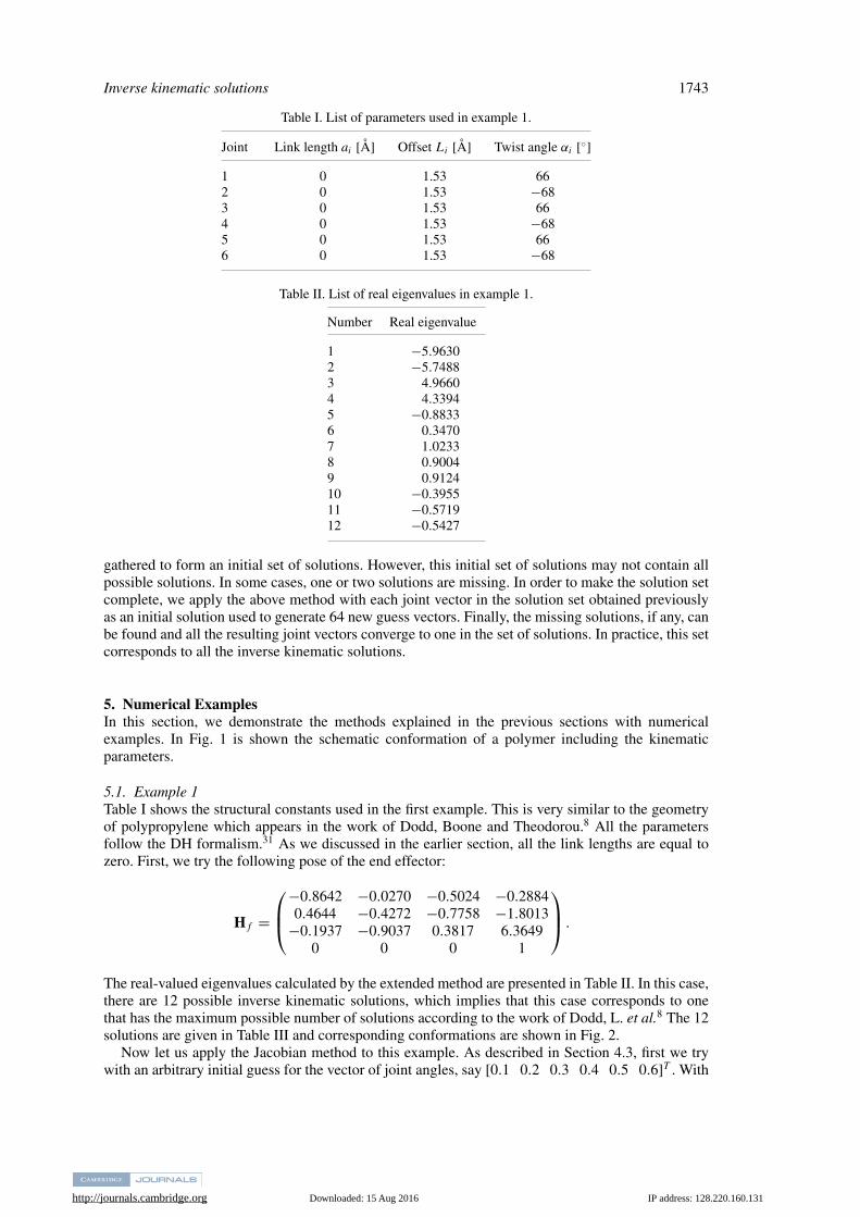
5.1. Example 1Table I shows the structural constants used in the first example. This is very similar to the geometryof polypropylene which appears in the work of Dodd, Boone and Theodorou.8 All the parametersfollow the DH formalism.31 As we discussed in the earlier section, all the link lengths are equal tozero. First, we try the following pose of the end effector:

Hf =

⎛⎜⎝

−0.8642 −0.0270 −0.5024 −0.28840.4644 −0.4272 −0.7758 −1.8013

−0.1937 −0.9037 0.3817 6.36490 0 0 1

⎞⎟⎠ .

The real-valued eigenvalues calculated by the extended method are presented in Table II. In this case,there are 12 possible inverse kinematic solutions, which implies that this case corresponds to onethat has the maximum possible number of solutions according to the work of Dodd, L. et al.8 The 12solutions are given in Table III and corresponding conformations are shown in Fig. 2.

Now let us apply the Jacobian method to this example. As described in Section 4.3, first we trywith an arbitrary initial guess for the vector of joint angles, say [0.1 0.2 0.3 0.4 0.5 0.6]T . With




Table III. The joint angles corresponding to the solutions [◦].

i θ1 θ2 θ3 θ4 θ5 θ6

1 −96.2800 −26.2700 −160.9600 38.4800 82.5500 −35.40002 81.9899 4.9596 −160.2643 −60.3541 −68.3477 −34.03013 −82.7885 −3.1069 157.2294 63.1350 88.3393 −29.67534 94.1134 29.5025 154.0461 −37.6020 −57.6850 −26.10635 6.4869 −62.1639 −82.9073 −137.4351 −1.1064 28.10576 −4.0928 66.6818 38.2765 −138.3936 −44.1007 −131.78767 −86.6833 −7.3910 91.3207 −56.8352 −87.9667 −103.51528 80.9276 62.1464 84.0005 −62.0489 −1.7489 27.41609 11.3907 78.4807 84.7535 135.6536 2.1915 −107.775210 34.5097 −35.7504 −43.1578 118.9050 52.5449 49.073811 −65.4235 −77.5112 −59.5267 87.4006 −13.2471 −122.374612 59.9160 −14.5902 −56.9800 91.1014 65.9502 42.8249

Fig. 2. The conformations of all the solutions in example 1.

the same geometric parameters and pose of the end effector as in the above example, we can get oneinverse kinematic solution as

θ =

⎛⎜⎜⎜⎜⎜⎝

−82.7885−3.1069157.229463.135088.3393

−29.6753

⎞⎟⎟⎟⎟⎟⎠ .




Table IV. Comparison of running time.

Average (± std) [sec] Extended elimination method Jacobian method

Example 1 3.4771 × 10−3(±4.4242 × 10−4) 0.1181(±6.6641 × 10−3)Example 2 3.2032 × 10−3(±2.4787 × 10−4) 0.1219(±6.9362 × 10−3)

(5.4271 × 10−3(±5.6102 × 10−4))∗

Example 3 3.4367 × 10−3(±5.5903 × 10−4) 0.1218(±6.7818 × 10−3)

∗Combined method

With this vector as an initial guess vector, we try the Jacobian method for the 64 different cases. Inthis example, fortunately we can generate 12 inverse kinematic solutions with only one initial guessvector. The results are exactly the same as in Table III and Fig. 2. However, in general, we shouldapply this method for each of the resulting set of vectors as an initial guess vector. It is worth notingthat, when we add 0, π/2, π , and 3π/2 instead of 0 and π , we obtain the same solution sets for allthe examples in this section. This illustrates that the Jacobian method is practically good enough toobtain all inverse kinematic solutions.

As one can imagine, the Jacobian method should be slower than the extended elimination method,in part due to the iterative computation. In order to compare the computational efficiency betweentwo methods, we measured time spent for each method, as respectively explained in Sections 3.1and 4.3. Each method was implemented via Matlab script files to run in Matlab (version R2015) ona laptop computer (CPU 2.3 GHz Intel Core i7, OS X 10.10.4). To optimize the performance, thecomputationally heaviest parts (the part that finds all solutions in the extended elimination method,and the iteration part with 64 different initial sets in the Jacobian method) are replaced by C using“mex” function in Matlab. Twenty trials were performed for each method. Computation times werethen measured by using “tic/toc” Matlab commands. Table IV shows the average computation timesfor the extended method and the Jacobian method for example 1, 2 and 3, respectively, in the formatof average (± standard deviation). For all cases, the average computation times for the extendedelimination method and the Jacobian method are about 3 × 10−3 and 0.1 s, respectively. Note thatin the table, the case marked with an asterisk in Example 2 corresponds to the combined methodthat applies the extended elimination and the Jacobian methods together, which is useful in specialsituations that will be explained in more detail in the next example. The results clearly show that thatthe Jacobian method is computationally much more expensive than the extended elimination method.This is one drawback of the Jacobian method. However, as we will see in the following example, wecan make use of the Jacobian method for a special purpose.

Note that, although we optimized our Matlab codes using “mex” function, it is difficult to directlycompare the computational speed with other methods11, 52, 53 partly due to the availability of theexisting codes and some of them being written entirely in Fortran, C and python. Also, the technicalskill of writing different codes in different languages becomes another factor that adds up to thisdifficulty. Finally, unlike the methods mentioned above, our method is to obtain all the possibleconformations of 6-degree-of-freedom biopolymer structure. That being said, we believe that ourapproach, especially the eigenvalue approach, is at least as fast as other well-known methods especiallyin terms of obtaining all the possible conformations, because there is no iterative procedure involvedand the dimension of the matrix for eigenvalue problem is the smallest among known ones.

5.2. Example 2As the next numerical example, we consider the case which appears in Table V. This is similar to thesimplified model of a protein molecule,9, 10 except that the C − N bond is not fixed as 180◦. Althougheach bond length of a backbone in a molecule can vary within some range, we treat here the bondlength between each atom in a backbone as a covalent bond which has same bond length with 1.5 A.59

Let the pose of an end effector be

Hf =

⎛⎜⎝

0.5681 −0.7792 −0.2647 4.3548−0.0992 0.2544 −0.9620 −0.56970.8169 0.5728 0.0672 1.0536

0 0 0 1.0000

⎞⎟⎠ .




Table V. List of parameters used in example 2.


1 0 1.5 602 0 1.5 −603 0 1.5 70.534 0 1.5 −605 0 1.5 606 0 1.5 −70.53

Table VI. List of real eigenvalues in example 2.

Number Real eigenvalues

1 5.99702 −2.97243 0.95904 0.8375

Table VII. The joint angles by the extended elimination method in example 2 [◦].

i θ1 θ2 θ3 θ4 θ5 θ6

1 166.3421 130.8356 161.0662 99.6300 0.6208 67.25852 14.2311 −93.6975 −142.8117 79.5403 131.5450 −161.21733 −148.7040 65.5293 87.6000 2.2625 29.2118 79.23194 43.2346 −37.7975 79.8894 −156.3153 64.0651 −133.0993

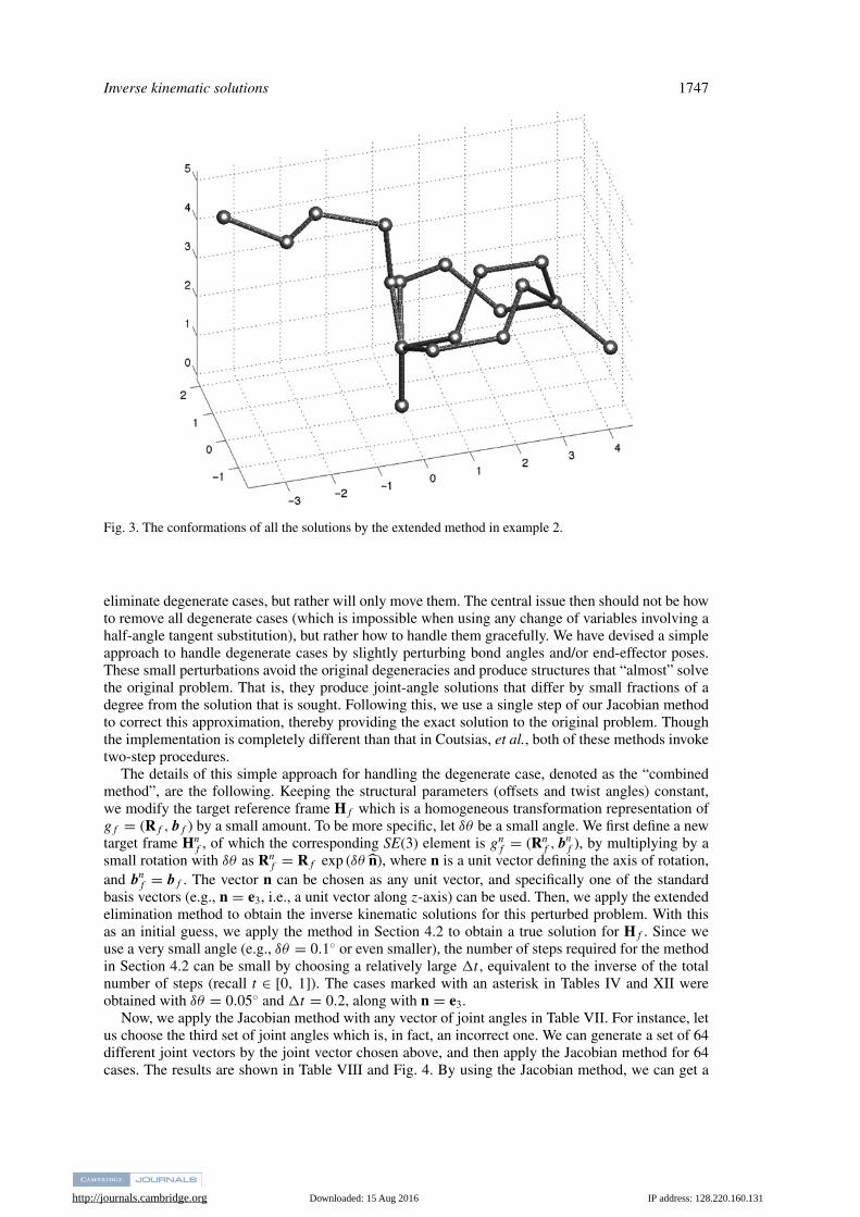
First, we apply the extended method to this example. Solving the eigenvalue problem of Eq. (13)gives four distinct real eigenvalues, which are shown in Table VI. In Table VII are shown the jointangles as well. In addition, Fig. 3 shows the conformations of each solution. Looking at Fig. 3, wecan see that one of four solutions is not a true solution, which corresponds to the third real eigenvalue,0.9590. If we further look at the last element of the corresponding eigenvector, which is to be usedfor normalization, it is −2 × 10−14. In addition to the last element, we see that 17 elements arenearly zeros. Hence, normalizing this eigenvector leads to the incorrect answer. Actually, since thelast element can be treated as zero, we should not normalize this eigenvector.

Note that there has been some work on using polynomial root finding for inverse kinematicsolutions in the case when some joint angles are 180◦ (e.g., Manseur and Doty21). However, thework considered general robot manipulator geometries which did not include the special case ofbiopolymer structures. Other methods presented in the literature also have degeneracies. The methodof Manocha, et al.25 suffers from the same numerical issues as ours when some of the joint angles are180◦. The method of Coutsias, et al.11 describes a polypeptide chain as a series of virtual Cα − Cα

bonds, and instead of using the original torsion angles it concentrates the degrees of freedom asspherical rotations at each vertex where virtual bonds are connected. The actual bonds and bondangles can then be reconstructed after the inverse kinematics solution for the virtual structure isfound. Essentially this method substitutes the original polypeptide chain with a nonphysical proxy.Then, it solves the inverse kinematics problem for this proxy, and fits the pieces of the originalstructure to it in a second procedure. The non-linear change of coordinates employed in this approachdistorts the original kinematics problem, and as such, does not have all of the same degenerate cases.However, this does not mean that it is free of degeneracies. As an analogy, the Jacobian matrix for any6-D.O.F. manipulator will have singularities somewhere in the configuration space, and switchingfrom one kinematic structure to another will not eliminate singularities, but rather will only movethem to new locations. Likewise, using a non-physical proxy structure in place of the original will not




Fig. 3. The conformations of all the solutions by the extended method in example 2.

eliminate degenerate cases, but rather will only move them. The central issue then should not be howto remove all degenerate cases (which is impossible when using any change of variables involving ahalf-angle tangent substitution), but rather how to handle them gracefully. We have devised a simpleapproach to handle degenerate cases by slightly perturbing bond angles and/or end-effector poses.These small perturbations avoid the original degeneracies and produce structures that “almost” solvethe original problem. That is, they produce joint-angle solutions that differ by small fractions of adegree from the solution that is sought. Following this, we use a single step of our Jacobian methodto correct this approximation, thereby providing the exact solution to the original problem. Thoughthe implementation is completely different than that in Coutsias, et al., both of these methods invoketwo-step procedures.

The details of this simple approach for handling the degenerate case, denoted as the “combinedmethod”, are the following. Keeping the structural parameters (offsets and twist angles) constant,we modify the target reference frame Hf which is a homogeneous transformation representation ofgf = (Rf , bf ) by a small amount. To be more specific, let δθ be a small angle. We first define a newtarget frame Hn

f , of which the corresponding SE(3) element is gnf = (Rn

f , bnf ), by multiplying by a

small rotation with δθ as Rnf = Rf exp (δθ n), where n is a unit vector defining the axis of rotation,

and bnf = bf . The vector n can be chosen as any unit vector, and specifically one of the standard

basis vectors (e.g., n = e3, i.e., a unit vector along z-axis) can be used. Then, we apply the extendedelimination method to obtain the inverse kinematic solutions for this perturbed problem. With thisas an initial guess, we apply the method in Section 4.2 to obtain a true solution for Hf . Since weuse a very small angle (e.g., δθ = 0.1◦ or even smaller), the number of steps required for the methodin Section 4.2 can be small by choosing a relatively large �t , equivalent to the inverse of the totalnumber of steps (recall t ∈ [0, 1]). The cases marked with an asterisk in Tables IV and XII wereobtained with δθ = 0.05◦ and �t = 0.2, along with n = e3.

Now, we apply the Jacobian method with any vector of joint angles in Table VII. For instance, letus choose the third set of joint angles which is, in fact, an incorrect one. We can generate a set of 64different joint vectors by the joint vector chosen above, and then apply the Jacobian method for 64cases. The results are shown in Table VIII and Fig. 4. By using the Jacobian method, we can get a




Table VIII. The joint angles by the Jacobian method in example 2 [◦].

i θ1 θ2 θ3 θ4 θ5 θ6

1 166.3421 130.8356 161.0662 99.6300 0.6208 67.25852 14.2311 266.3025 217.1883 79.5403 131.5450 198.78273 143.3000 180.0000 87.6000 180.0000 323.5000 38.30004 43.2346 322.2025 79.8894 203.6847 64.0651 226.9007

Table IX. List of DH parameters for protein structures. This isadopted from Manocha, et al.25.


1 0 −5.81 8.672 0 9.44 70.053 0 −5.86 8.614 0 9.49 70.115 0 −5.78 8.686 0 9.42 70.12

Fig. 4. The true inverse kinematic solutions in example 2.

set of solutions with true joint angle vectors, which the extended elimination method does not give.Looking at Fig. 4, we can see that all four of the solutions are correct.

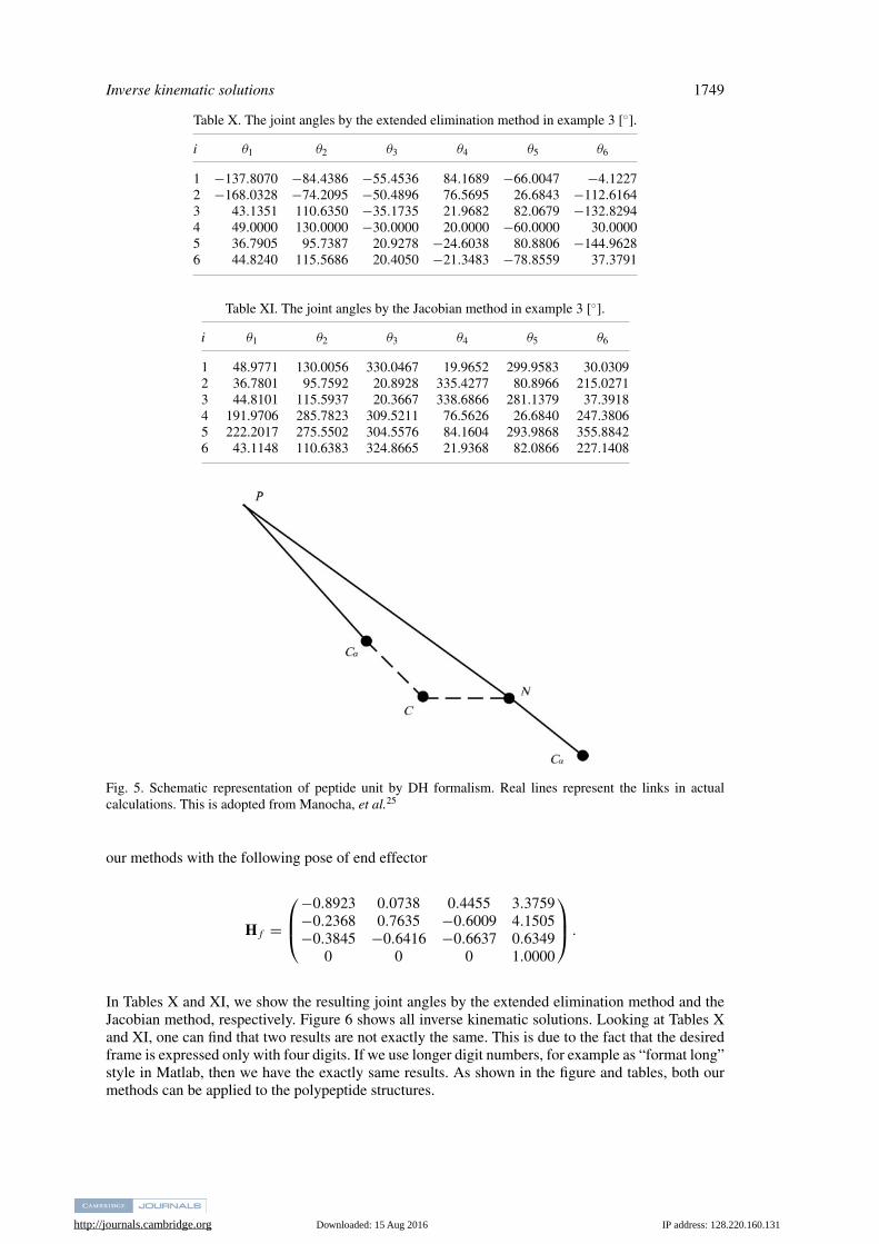
5.3. Example 3As the third example, we consider the polypeptide structure. In Fig. 5 is depicted the schematic pictureof a polypeptide unit, which is adopted from Manocha, et al..25 All four atoms in the peptide unit,such as Cα , C and N , lie in the same plane. Noting that the each link P − Cα has the same rotationwith Cα − C and N − Cα , we can treat those two as the links in DH formalism. All DH parametersare shown in Table IX. Originally, this data was obtained from a segment of α helix.25 Then, we apply




Table X. The joint angles by the extended elimination method in example 3 [◦].

i θ1 θ2 θ3 θ4 θ5 θ6

1 −137.8070 −84.4386 −55.4536 84.1689 −66.0047 −4.12272 −168.0328 −74.2095 −50.4896 76.5695 26.6843 −112.61643 43.1351 110.6350 −35.1735 21.9682 82.0679 −132.82944 49.0000 130.0000 −30.0000 20.0000 −60.0000 30.00005 36.7905 95.7387 20.9278 −24.6038 80.8806 −144.96286 44.8240 115.5686 20.4050 −21.3483 −78.8559 37.3791

Table XI. The joint angles by the Jacobian method in example 3 [◦].

i θ1 θ2 θ3 θ4 θ5 θ6

1 48.9771 130.0056 330.0467 19.9652 299.9583 30.03092 36.7801 95.7592 20.8928 335.4277 80.8966 215.02713 44.8101 115.5937 20.3667 338.6866 281.1379 37.39184 191.9706 285.7823 309.5211 76.5626 26.6840 247.38065 222.2017 275.5502 304.5576 84.1604 293.9868 355.88426 43.1148 110.6383 324.8665 21.9368 82.0866 227.1408

Fig. 5. Schematic representation of peptide unit by DH formalism. Real lines represent the links in actualcalculations. This is adopted from Manocha, et al.25

our methods with the following pose of end effector

Hf =

⎛⎜⎝

−0.8923 0.0738 0.4455 3.3759−0.2368 0.7635 −0.6009 4.1505−0.3845 −0.6416 −0.6637 0.6349

0 0 0 1.0000

⎞⎟⎠ .

In Tables X and XI, we show the resulting joint angles by the extended elimination method and theJacobian method, respectively. Figure 6 shows all inverse kinematic solutions. Looking at Tables Xand XI, one can find that two results are not exactly the same. This is due to the fact that the desiredframe is expressed only with four digits. If we use longer digit numbers, for example as “format long”style in Matlab, then we have the exactly same results. As shown in the figure and tables, both ourmethods can be applied to the polypeptide structures.




Table XII. Results of example 4 (tripzip2 case): original structures.

Extended elimination method Jacobian method

Trials # of solutions Computing time [s] # of solutions Computing time [s]

1 1 (2) 2.5757 × 10−3 (± 8.4090 × 10−5) 2 0.1122 (± 5.6673 × 10−3)2

(4.9820 × 10−3 (± 2.9500 ± 10−4)

)∗

2 6 2.6067 × 10−3 (± 9.9450 × 10−5) 6 0.0938 (± 3.4573 × 10−3)3 4 2.6304 × 10−3 (± 2.6050 × 10−4) 4 0.1086 (± 2.9198 × 10−3)4 2 2.6527 × 10−3 (± 3.1320 × 10−4) 2 0.1025 (± 2.7672 × 10−3)5 6 2.6285 × 10−3 (± 1.5590 × 10−4) 6 0.0960 (± 3.5481 × 10−3)6 4 2.5773 × 10−3 (± 7.5420 × 10−5) 4 0.1023 (± 2.4818 × 10−3)7 2 2.5684 × 10−3 (± 7.5904 × 10−5) 2 0.1256 (± 3.0442 × 10−3)8 2 2.5541 × 10−3 (± 6.5750 × 10−5) 2 0.1053 (± 2.2375 × 10−3)

∗Combined method

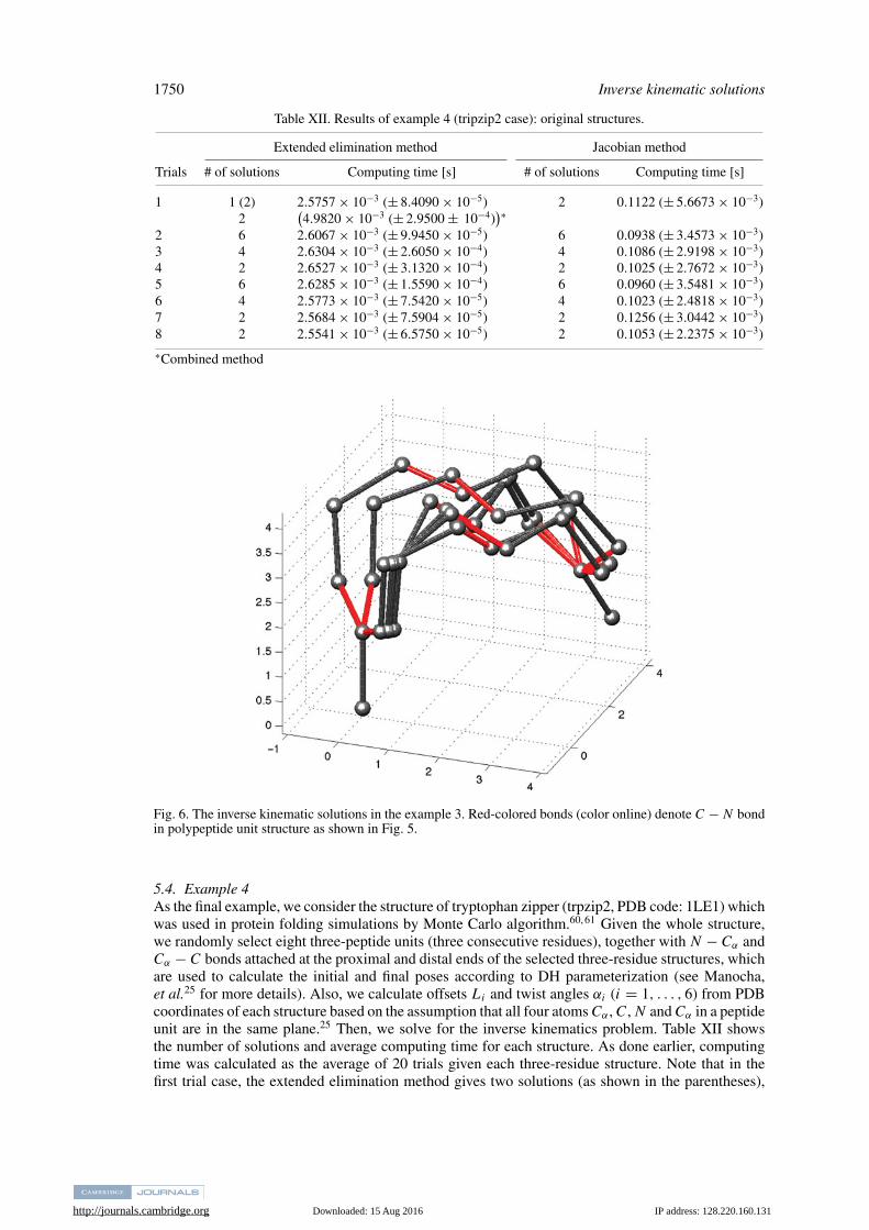
Fig. 6. The inverse kinematic solutions in the example 3. Red-colored bonds (color online) denote C − N bondin polypeptide unit structure as shown in Fig. 5.

5.4. Example 4As the final example, we consider the structure of tryptophan zipper (trpzip2, PDB code: 1LE1) whichwas used in protein folding simulations by Monte Carlo algorithm.60, 61 Given the whole structure,we randomly select eight three-peptide units (three consecutive residues), together with N − Cα andCα − C bonds attached at the proximal and distal ends of the selected three-residue structures, whichare used to calculate the initial and final poses according to DH parameterization (see Manocha,et al.25 for more details). Also, we calculate offsets Li and twist angles αi (i = 1, . . . , 6) from PDBcoordinates of each structure based on the assumption that all four atoms Cα , C, N and Cα in a peptideunit are in the same plane.25 Then, we solve for the inverse kinematics problem. Table XII showsthe number of solutions and average computing time for each structure. As done earlier, computingtime was calculated as the average of 20 trials given each three-residue structure. Note that in thefirst trial case, the extended elimination method gives two solutions (as shown in the parentheses),




Table XIII. Results of example 4 (tripzip2 case): perturbed structures.

The extended method Jacobian method

Trials # of solutions Computing time # of solutions Computing time

1 2 2.5613 × 10−3 (± 7.1410 × 10−5) 2 0.1115 (± 3.5357 × 10−3)2 6 2.7044 × 10−3 (± 3.7720 × 10−4) 6 0.0940 (± 2.6699 × 10−3)3 4 2.6775 × 10−3 (± 3.4480 × 10−4) 4 0.1051 (± 3.2846 × 10−3)4 2 2.6183 × 10−3 (± 7.6130 × 10−5) 2 0.1073 (± 1.7974 × 10−3)5 6 2.6157 × 10−3 (± 9.8490 × 10−5) 6 0.1005 (± 2.2602 × 10−3)6 4 2.6847 × 10−3 (± 3.7270 × 10−4) 4 0.1031 (± 2.6349 × 10−3)7 4 2.6086 × 10−3 (± 8.4520 × 10−5) 4 0.0946 (± 2.6288 × 10−3)8 2 2.6531 × 10−3 (± 2.3180 × 10−4) 2 0.1012 (± 2.9837 × 10−3)

but one of them is not correct because one of joint angles become very close to 180◦ (180.01◦as obtained by the Jacobian method which could give all correct solutions). When we apply thecombined method, then we could obtain two correct solutions again with a computation time almostas good as the extended elimination method alone (marked with an asterisk in Table 5.3). After that,we apply a slight angular perturbation (5◦) about N − Cα attached at the proximal end, and applyour methods to obtain the inverse kinematic solutions. This process is to mimic “concerted rotations”moves used in Monte Carlo simulations for chainlike molecules. This small perturbation affects theinitial pose of the chosen polypeptide structure, but we keep the final pose fixed, to seek the inversekinematic solutions. Table XIII shows the results of the perturbation (the number of solutions andaverage computing time). In total, this example emphasizes the versatility of our methods even inmore realistic situations.

6. ConclusionsIn this paper, we have presented two methods for finding all the possible conformations of short end-constrained segments of polymers such as polypeptides and polypropylene. These segments have sixfree joint angles (dihedral angles) with end constraints in position and orientation. As for the firstmethod in this paper, we have adopted and modified concepts from the inverse kinematics of thegeneral 6R manipulator, which break down in the case of polymer geometries. We have extendedan elimination method based on the work of Kohli and Osvatic which is suitable for the degenerategeometry that polymers usually have. We have also developed a heuristic Jacobian-based method,which can be implemented easily not only for a polymer but also for the general 6R manipulatorin that it does not require any symbolic computations. This method utilizes an artificial path inEuclidean motion group. We compared the computational performance of these methods and foundthat the extended elimination method is computationally more favorable than the Jacobian method.However, when it comes to the kinematically degenerate cases such as when some of the joint anglesare equal to 180◦, the Jacobian method gives accurate solutions whereas the extended eliminationmethod cannot. We have also presented the combined method which utilizes the extended methodand the Jacobian method efficiently in degenerate cases. This method, which could generate allcorrect solutions in degenerate cases, is shown to be as efficient as the extended method in terms ofcomputational speed. We have demonstrated this usefulness with appropriate numerical examples.We expect that our method can be applied to the protein folding algorithms and protein engineeringsuch as drug design.

AcknowledgmentsThis work was supported by the National Institute of General Medical Sciences of the NationalInstitutes of Health under award number R01GM113240. G. Chirikjian’s contribution to this workwas supported by the NSF IR/D program while serving as a program director under an IPAcontract. The ideas are expressed by the authors and do not necessarily express those of theNSF.




References1. G. Favrin, A. Irback and F. Sjunnesson, “Monte Carlo update for chain molecules: Biased Gaussian steps

in torsional space,” J. Chem. Phys. 114, 8154–8158 (2001).2. J. P. Ulmschneider and W. L. Jorgensen, “Monte Carlo backbone sampling for polypeptides with variable

bond angles and dihedral angles using concerted rotations and a Gaussian bias,” J. Chem. Phys. 118,4261–4271 (2003).

3. J. P. Ulmschneider and W. L. Jorgensen, “Monte Carlo backbone sampling for nucleic acids using concertedrotations including variable bond angles,” J. Phys. Chem. 108(43), 16883–16892 (2004).

4. D. Frenkel and B. Smit, Understanding Molecular Simulation (Academic Press, San Diego, 2002).5. N. Go and H. A. Scheraga, “Ring closure and local conformational deformations of chain molecules,”

Macromolecules 3, 178–187 (1970).6. N. Go and H. A. Scheraga, “Ring closure in chain molecules with Cn, I , or S2n symmetry,” Macromolecules

6, 273–281 (1973).7. N. Go and H. A. Scheraga, “Calculation of the conformation of cyclo-hexaglycyl,” Macromolecules 6,

525–535 (1973).8. L. Dodd, T. Boone and D. Theodorou, “A concerted rotation algorithm for atomistic Monte Carlo

simulations of polymer melts and glasses,” Mol. Phys. 78, 961–996 (1993).9. E. Knapp, “Long time dynamics of a polymer with rigid body monomer units relating to a protein model:

Comparison with the Rouse model,” J. Comput. Chem. 13, 793–798 (1992).10. E. Knapp and A. Irgens-Defregger, “Off-lattice Monte Carlo method with constraints: Long-time dynamics

of a protein model without nonbonded interactions,” J. Comput. Chem. 14, 19–29 (1993).11. E. A. Coutsias, C. Seok, M. P. Jacobson and K. A. Dill, “A kinematic view of loop closure,” J. Comput.

Chem. 25, 510–528 (2004).12. C. H. Mak, “RNA conformational sampling: 1. Single-nucleotide loop closure,” J. Comput. Chem. 29,

926–933 (2008).13. C. H. Mak, W-Y. Chung and N. D. Markovskiy, “RNA conformational sampling II: Arbitrary length

multinucleotide loop closure,” J. Chem. Theory Comput. 7, 1198–1207 (2011).14. W. Wedemeyer and H. A. Scheraga, “Exact analytical loop closure in prsotein using polynomial equations,”

J. Comput. Chem. 20, 819–844 (1999).15. H. Lee and C. Liang, “A new vector theory for the analysis of spatial mechanism,” Mech. Mach. Theory

23, 209–217 (1988).16. H. Lee and C. Liang, “Displacement analysis of the general spatial 7-link 7R mechanism,” Mech. Mach.

Theory 23, 219–226 (1988).17. D. Manocha and J. Canny, “Efficient inverse kinematics for general 6R manipulators,” IEEE Trans. Robot.

Autom. 10, 648–657 (1994).18. M. G. Wu and M. W. Deem, “Analytical rebridging Monte Carlo: Application to cis/trans isomerization

in proline-containing, cyclic peptides,” J. Chem. Phys. 111, 6625–6632 (1999).19. J. Duffy and C. Crane, “A displacement analysis of the general spatial 7R mechanisms,” Mech. Mach.

Theory 15, 153–169 (1980).20. L-W. Tsai and A. Morgan, “Solving the kinematics of the most general six- and five-degree-of-

freedom manipulators by continuation methods,” ASME J. Mech. Transm. Autom. Des. 107, 189–200(1985).

21. R. Manseur and K. L. Doty, “A robot manipulator with 16 real inverse kinematic solution sets,” Int. J.Robot. Res. 8(5), 75–79 (1989).

22. C. Wampler and A. Morgan, “Solving the 6R inverse position problem using a generic-case solutionmethodology,” Mech. Mach. Theory 26(1), 91–106 (1991).

23. M. Raghavan and B. Roth, “Kinematic analysis of the 6R manipulator of general geometry,” In:Proceedings of the 5th International Symposium on Robotics Research (H. Miura and S. Airmoto, eds.)(MIT Press, Cambridge, MA, 1990) pp. 263–270.

24. M. Raghavan and B. Roth, “Kinematic analysis of the 6R manipulator and related linkages,” ASME J.Mech. Des. 115, 502–508 (1993).

25. D. Manocha, Y. Zhu and W. Wright, “Conformational analysis of molecular chains using nano-kinematics,”Comput. Appl. Biosci. 11, 71–86 (1995).

26. D. Kohli and M. Osvatic, “Inverse kinematics of the general 6R and 5R,P serial manipulators,” ASME J.Mech. Des. 115, 922–931 (1993).

27. M. Ghazvini, “Reducing the Inverse Kinematics of Manipulators to the Solution of a GeneralizedEigenproblem,” In: Computational Kimematics (J. Angeles, et al., ed.) (Kluwer Academic Publishers,Springer, Netherlands, 1993) pp. 15–26.

28. J. Nielson and B. Roth, “On the kinematic analysis of robotic mechanisms,” Int. J. Robot. Res. 12(12),1147–1160 (1999).

29. M. L. Husty, M. Pfurner and H-P. Schrocker, “A new and efficient algorithm for the inverse kinematics ofa general serial 6R manipulator,” Mech. Mach. Theory 42(1), 66–81 (2007).

30. T. Rudny, “Solving inverse kinematics by fully automated planar curves intersecting,” Mech. Mach. Theory74, 310–318 (2014).

31. M. Spong and M. Vidyasagar, Robot Dynamics and Control (John Wiley and Sons, New York, 1989).32. G. Golub and C. Van Loan, Matrix Computations (The Johns Hopkins University Press, Baltimore, 1996).33. E. Anderson et al., LAPACK User’s Guide (SIAM, Philadelphia, PA, 1999).




34. M. McCarthy, An Introduction to Theoretical Kinematics (MIT Press, Cambridge, MA, 1990).35. M. Murray, Z. Li and S. Sastry, A Mathematical Introduction to Robotic Manipulation (CRC Press, Boca

Raton, 1994).36. G. S. Chirikjian and A. B. Kyatkin, Engineering Applications of Noncommutative Harmonic Analysis

(CRC Press, Boca Raton, FL, 2001).37. A. J. Sommese and C. W. Wampler, The Numerical Solution to Systems of Polynomials Arising in

Engineering and Science (World Scientific, Singapore, 1985).38. A. Morgan, Solving Polynomial Systems Using Contiuation For Engineering and Scientific Problems

(Prentice-Hall, New Jersey, 1987).39. I. Ebert-Uphoff and G. S. Chirikjian, “Inverse kinematics of discretely actuated hyper-redundant

manipulators using workspace densities,” Proceedings of the IEEE International Conference on Roboticsand Automation (Minneapolis, MN, 1996) pp. 139–145.

40. G. S. Chirikjian, “Inverse kinematics of binary manipulators using a continuum model,” J. Intell. Robot.Syst. 19, 5–22 (1997).

41. J. Suthakorn and G. S. Chirikjian, “A new inverse kinematics algorithm for binary manipulators withmany actuators,” Adv. Robot. 15(2), 225–244 (2001).

42. Y. Wang and G. S. Chirikjian, “Workspace generation of hyper-redundant manipulators as a diffusionprocess on SE(N),” IEEE Trans. Robot. Autom. 20(3), 399–408 (2004).

43. A. B. Kyatkin and G. S. Chirikjian, “Computation of robot configuration and workspaces via the fouriertransform on the discrete motion group,” Int. J. Robot. Res. 18(6), 601–615 (1999).

44. Y. Wang, “A fast workspace-density-driven inverse kinematics method for hyper-redundant manipulators,”Robotica 24, 649–655 (2006).

45. G. S. Chirikjian, “Conformational statistics of macromolecules using generalized convolution,” Comput.Theor. Polym. Sci. 11, 143–153 (2001).

46. J. S. Kim and G. S. Chirikjian, “A unified approach to conformational statistics of classical polymer andpolypeptide models,” Polymer 46, 11904–11917 (2005).

47. D. Whitney, “Resolved motion rate control of manipulators and human prostheses,” IEEE Trans. Man-Mach. Syst. MMS-10(2), 47–53 (1969).

48. J. Uicker, J. Denavit and R. Hartenberg, “An iterative method for the displacement analysis of spatialmechanisms,” ASME J. Appl. Mech. 107, 189–200 (1954).

49. T. Isobe, K. Nagasaka and S. Yamamoto, “A new approach to kinematic control of simple manipulators,”IEEE Trans. Syst. Man Cybern. 22(5), 1116–1124 (1992).

50. L. Wang and C. Chen, “A combined optimization method for solving inverse kinematics problem ofmechanical manipulators,” IEEE Trans. Robot. Autom. 7(4), 489–499 (1991).

51. A. L. Olsen and H. G. Petersen, “Inverse kinematics by numerical and analytical cyclic coordinate descent,”Robotica 29(4), 619–626 (2011).

52. A. Canutescu and R. Dunbrack, “Cyclic coordinate descent: A robotic algorithm for protein loop closure,”Protein Sci. 12, 963–972 (2003).

53. W. Boomsma and T. Hamelryck, “Full cyclic coordinate descent: Solving the protein loop closure problemin Cα space,” BMS Bioinformatics 6, 159 (2005).

54. K. Al-Nasr and J. He, “An effective convergence independent loop closure method using forward-backwardcyclic coordinate descent,” Int. J. Data Min. Bioinformatics 3(3), 346–361 (2009).

55. J. S. Kim and G. S. Chirikjian, “Conformational analysis of stiff chiral polymers with end-constraints,”Mol. Simul. 32(14), 1139–1154 (2006).

56. F. C. Park, “Distance metrics on the rigid-body motions with applications to mechanism design,” J. Mech.Des. 117, 48–54 (1995).

57. G. S. Chirikjian and S. Zhou, “Metrics on motion and deformation of solid models,” J. Mech. Des. 120(2),252–261 (1998).

58. G. S. Chirikjian and Y. Yan, “Mathematical aspects of molecular replacement. II. Geometry of motionspaces,” Acta Cryst. A68, 208–221 (2012).

59. B. Alberts, A. Johnson, J. Lewis, M. Raff, K. Roberts and P. Walter, Molecular Biology of the Cell (GarlandScience, New York, 2000).

60. J. P. Ulmschneider and W. L. Jorgensen, “Polypeptide folding using Monte Carlo sampling, concertedrotation, and continuum solvation,” J. Am. Chem. Soc. 126, 1849–1857 (2004).

61. J. P. Ulmschneider and W. L. Jorgensen, “Monte Carlo vs molecular dynamics for all-atom polypeptidefolding simulations,” J. Phys. Chem. B 110, 16733–16742 (2006).


Date post:	28-May-2020
Category:	Documents
Upload:	others
View:	3 times
Download:	0 times

Robotica //rpk.lcsr.jhu.edu/wp-content/uploads/2016/08/Kim16_Inverse... · Robotica Additional...

Documents