Robust Real-time Extraction of Fiducial Facial

Feature Points using Haar-like Features Harry Commin

MEng in Electrical & Electronic Engineering with Year Abroad

Final Year Project Report 2009

Dept. of Electrical & Computer Engineering, National University of Singapore

Dept. of Electrical & Electronic Engineering, Imperial College London

Abstract

In this paper, we explore methods of robustly extracting fiducial facial feature

points – an important process for numerous facial image processing tasks. We consider

various methods to first detect face, then facial features and finally salient facial feature

points. Colour-based models are analysed and their overall unsuitability for this task is

summarised. The bulk of the report is then dedicated to proposing a learning-based

method centred on the Viola-Jones algorithm. The specific difficulties and considerations

relating to feature point detection are laid out in this context and a novel approach is

established to address these issues.

On a sequence of clear and unobstructed face images, our proposed system

achieves average detection rates of over 90%. Then, using a more varied sample dataset,

we identify some possible areas for future development of our system.

Acknowledgements

I would like to thank my supervisor, Prof. Ge, for providing a lab that was

available day and night. The enthusiasm and keen work ethic of my lab colleagues was

also highly motivating.

For inspiring my now obsessive interest in human visual perception, I thank Dr.

Yen Shih-Cheng and his quite exceptional Biological Perception lectures. His insights

opened up a massive new perspective on my project and the world I perceive in general.

Finally, thanks go to Santosh Joshi for enriching my year with a colourful mix of

academic conversation and extracurricular mischief. The year could not have been the

same without the many late-night waffles and general laid-back good humour during

times of academic adversity.

Contents

1 Introduction .................................................................................................................................................................................................................................................................................................................................................................................................................... 1111

1.1 Project Motivation ...................................................................................................... 1

1.2 Background ................................................................................................................. 2

1.2.1 Colour-based Segmentation .............................................................................. 2

1.2.2 Template Matching ........................................................................................... 2

1.2.3 Feature Tracking ............................................................................................... 3

1.2.4 Neural Networks ............................................................................................... 3

1.2.5 Graph Matching ................................................................................................ 3

1.2.6 Eigenfaces .......................................................................................................... 4

1.2.7 Boosting ............................................................................................................. 5

1.2.8 Discussion of the Human Visual System .......................................................... 5

2 Technical Framework ....................................................................................... 7

2.1 Review of Colour-based Feature Point Detection ...................................................... 7

2.1.1 Research Context ................................................................................................. 7

2.1.2 Relating Back to the Human Visual System....................................................... 9

2.2 A Learning-based Approach ..................................................................................... 10

2.2.1 The Viola-Jones Algorithm ................................................................................ 10

2.2.2 Adaptations of Viola-Jones ................................................................................ 10

3 Implementation ................................................................................................ 17

3.1 Detector Structure .................................................................................................... 17

3.2 Design Considerations .............................................................................................. 18

3.3 Training .................................................................................................................... 21

3.3.1 Image Database ................................................................................................. 21

3.3.2 Positive Samples ................................................................................................ 22

3.3.3 Negative Samples .............................................................................................. 25

3.4 C++ Code Implementation ....................................................................................... 26

4 Results ................................................................................................................. 27

4.1 Testing Datasets ....................................................................................................... 27

4.2 Results from Marked-up Database .......................................................................... 28

4.3 Results from Non-marked Database ........................................................................ 29

4.3.1 Mouths ............................................................................................................... 30

4.3.2 Spectacles ........................................................................................................... 30

4.3.3 Fringe Hair ........................................................................................................ 32

4.3.4 Facial Hair ......................................................................................................... 32

5 Future Work and Conclusions ....................................................................... 33

5.1 Future Work ............................................................................................................. 33

5.2 Conclusions ............................................................................................................... 34

Bibliography ......................................................................................................... 35

Appendix A ............................................................................................................ 38

1

Chapter 1

Introduction

1.1 Project Motivation

Extracting salient facial feature points accurately and robustly is absolutely

fundamental to the success of the facial image processing system that is built upon

them. Such applications include face identification, facial expression recognition, face

tracking and lip reading [2]. These feature points generally provide the foundations for

the entire system and it is imperative, therefore, that stability and reliability are

maximised.

There is no single way to formally define the set of facial feature points, since

different applications will have different requirements. Various publications make use

of, for example 16 [1], 20 [2] or 34 [3] salient points. In general, these will include

distinctive points such as the corners of eyes, mouth and eyebrows – but the specific

details vary. Thus, it is desirable to develop an approach that is somewhat adaptable in

nature so it can be readily altered to achieve detection of any feature point.

In the past, many systems have ignored this step and relied upon manual

marking [3, 4, 5] in order to focus better on the overall system. However, in most cases,

it is necessary (or at least highly desirable) to achieve automated detection quickly, or

even in real-time. In other words, good detection performance is not the only concern – a

system capable of flawless feature point classification may be of little practical use if it

cannot meet real-time requirements. So, when choosing our approach, we will try to

identify methods that minimise computational complexity wherever possible.

So, the purpose of our work is to develop a method that allows real-time detection

of any facial feature point. We seek computational efficiency in order to achieve high

frame rate. Where possible, the system should be invariant to general changes within

the image, such as scale, translation, rotation and ambient lighting. Additionally, we

require robustness regardless of inter-subject differences, such as race, gender and age.

2

1.2 Background

The numerous methods that have been proposed to tackle facial feature point

detection problems can be roughly divided into two categories: texture-based and shape-

based. Texture-based approaches seek to model the texture properties in the local area

around a feature point according to pixel values. Shape-based methods make use of the

more general geometries of the face and features, according to some prior knowledge.

These two types of approach are by no means independent, and hybrid systems have

been shown to give strong results [14, 21].

We will review a few of the more common tools used in approaching the feature

point detection problem. This should provide some general insight and aid

understanding of the method we finally choose.

1.2.1 Colour-based Segmentation

This method is simple and intuitive. Pixels corresponding to skin tend to exist in

a relatively tight cluster in colour space, even with variation in race and lighting

conditions [11]. A statistical model of skin colour properties is obtained by analysing

databases of manually-segmented face images. This model is then used to estimate the

likelihood that a given pixel corresponds to skin. Various colour spaces (e.g. RGB, YUV,

HSL) and statistical models have been used in an attempt to improve classification

performance [8].

Features can then be located within the face through additional local analysis of

colour/intensity properties [16], or further image processing techniques such as

detection of edges and connectivity [9, 10].

1.2.2 Template Matching

In its simplest form, a template can be created by obtaining, for example, an

averaged intensity gradient map of a database of frontal face images [17]. Then,

detection is achieved by rescaling and shifting this template across a given frame’s

intensity gradient image, seeking the peak response.

In its basic form, this method is obviously heavily flawed. Searching every

possible scale and translation would be inefficient, but omitting any could cause spatial

inaccuracies. Furthermore, suitability for feature point detection is limited since there is

no particular allowance for variations in expression or pose.

A more sophisticated method is to use deformable templates, which permit

constrained inter- and intra-feature deformations according to a number of predefined

3

relationships [7]. However, initial localisation within the image remains an issue and so

this method is somewhat better suited to more constrained tasks such as handwritten

character recognition [18] and object tracking [7].

1.2.3 Feature Tracking

Although feature tracking is very much a separate problem to feature detection,

it can provide great support. For example, if the detection system is highly accurate but

slow, a high-speed tracking algorithm can speed up overall performance by reducing the

number of detection operations. Alternatively, if the detector is somewhat noisy, a

tracking technique such as deformable template matching can enforce geometric

constraints to improve performance [7]. Other tracking techniques are based on optical

flow methods such as the popular Lucas-Kanade algorithm [16].

1.2.4 Neural Networks

Neural networks offer exciting potential as feature point detectors as they are

very much predisposed to be effective pattern recognisers. This computational model is

basically inspired by the way that biological nervous systems, such as the brain, process

information. That is, with a large number of highly interconnected, simple elements

(neurons) that can function in parallel. These neurons are arranged and connected in a

specific way that allows them to solve a single specific task.

For example, a network can be trained to recognise a given pattern (by

redistributing input weights and/or altering threshold), such that it will correctly

categorise any of the training patterns. However, the real strength of neural networks is

how they cope with unfamiliar inputs. By applying a “firing rule” (such as Hamming

distance), a neural network can accurately deduce the category that the input pattern

most likely belongs to – even if this pattern was not included in training.

An excellent introduction to this topic can be found here: [12]. Further

considerations regarding application to feature detection are discussed here: [13].

1.2.5 Graph Matching

Unlike many other methods, graph matching offers the possibility to locate a face

and the features within it in a single stage. Indeed, the geometrical layout and specific

local properties of the features themselves help to directly describe the face.

4

In general, the attributes of the nodes of the graph are determined by a local

image property such as a Gabor wavelet transform [14]. The graph edges describe the

spatial displacement between the facial features. The model graph is then matched to

the data graph by maximising some graph similarity function. Exhaustively searching

for a match is time-consuming, so heuristic algorithms are generally used.

1.2.6 Eigenfaces[19]

With eigenfaces, we can begin our discussion of a really crucial topic in pattern

recognition – the high-dimensional feature space. This is an important concept, so we

will start with the very simple example of a 1x3 pixel greyscale image. Another way of

representing this image would be as a single point in 3D space, with the grey level at

each pixel determining progression along each axis.

Similarly, a 256x256 greyscale image can be represented as a single point in an

abstract 65,536-dimensional space. Now, if we plot a whole database of frontal face

images (equally scaled, rotated and centred) in this space, then, due to the similarities

between human faces, these points will not just be randomly distributed – they will be

somewhat clustered together. The clustering suggests that there is a substantial degree

of redundancy in this representation of the face.

This redundancy is important – it means that a relatively small number of

vectors are likely to contain a disproportionately large portion of a face’s inherent visual

characteristics. If we can somehow find a way of selecting these most important vectors,

then we can potentially discard all other data and therefore massively reduce the scope

of our problem.

In the case of Eigenfaces, the technique for selecting these vectors is Principal

Component Analysis (PCA). This method basically treats the training images as a group

of 1D vectors, forms their covariance matrix, then finds the eigenvectors (eigenfaces) of

this covariance matrix. The subspace described by these vectors therefore provides

maximal variance (and therefore minimal reconstruction error of the face images) [20].

Although PCA projections are optimal in terms of correlation, true detection

performance is heavily compromised by background conditions, such as lighting and

viewing direction. Various improvements and alternative dimensionality-reduction

techniques such as Fisher Linear Discriminant (fisherfaces), Indepenent Component

Analysis and Support Vector Machines have been proposed [22].

5

1.2.7 Boosting

Boosting is a machine learning algorithm that is often used in training object

detection systems. Rather like PCA, the objective of boosting is to select a relatively

small number of features that best describe the object we are trying to detect. However,

this method uses quite a different approach. With boosting, each feature is analysed

individually in terms of its classification performance.

In our context, we have a simple two-class classification problem – for example,

“eye” or “non-eye”. In order to categorise these, the boosting algorithm learns a number

of very simple “weak classifiers” and linearly combines them to form a strong classifier.

For our purposes, a weak classifier can be the boolean property of any simple image

feature – for example, a thresholded grey level value, or a thresholded filter response

centred at a certain pixel.

The great power of boosting is that these weak classifiers alone only need to be

slightly correlated with the true classification. For example, taking a database of known

“eye” samples and known “non-eye” samples, we may find that using a grey level

threshold of 100 at pixel coordinate (3, 5) will give correct classification 51% of the time.

Even though this feature is only a little better than random guessing, it can be linearly

combined with many other weak classifiers to achieve remarkable detection results.

Obviously, the example above is a very simple one. In practice, our image

features should be more sophisticated in order to encode more actual image detail. So,

we not only have to consider the boosting algorithm itself, but also the nature of the

features we use. These two factors will ultimately determine both detection performance

and computational complexity.

1.2.8 Discussion of the Human Visual System

While many of the above methods offer very interesting and innovative solutions,

it is not necessarily easy to know where to start. So, we will begin by focusing on the fact

that we really need to concentrate on elegance and simplicity. To this end, we can take

great inspiration from our own visual systems.

The task of facial feature point detection is really rather intuitive to us and yet

the range of tools available to our visual systems is somewhat basic. Our brains don’t

explicitly compute image transforms or edge maps; our monochromatic dark-adapted

vision doesn’t use any colour information at all. But still we outperform even the best

computer vision systems. So, it would be very interesting to briefly consider some of the

basic underlying neurological mechanisms it uses.

6

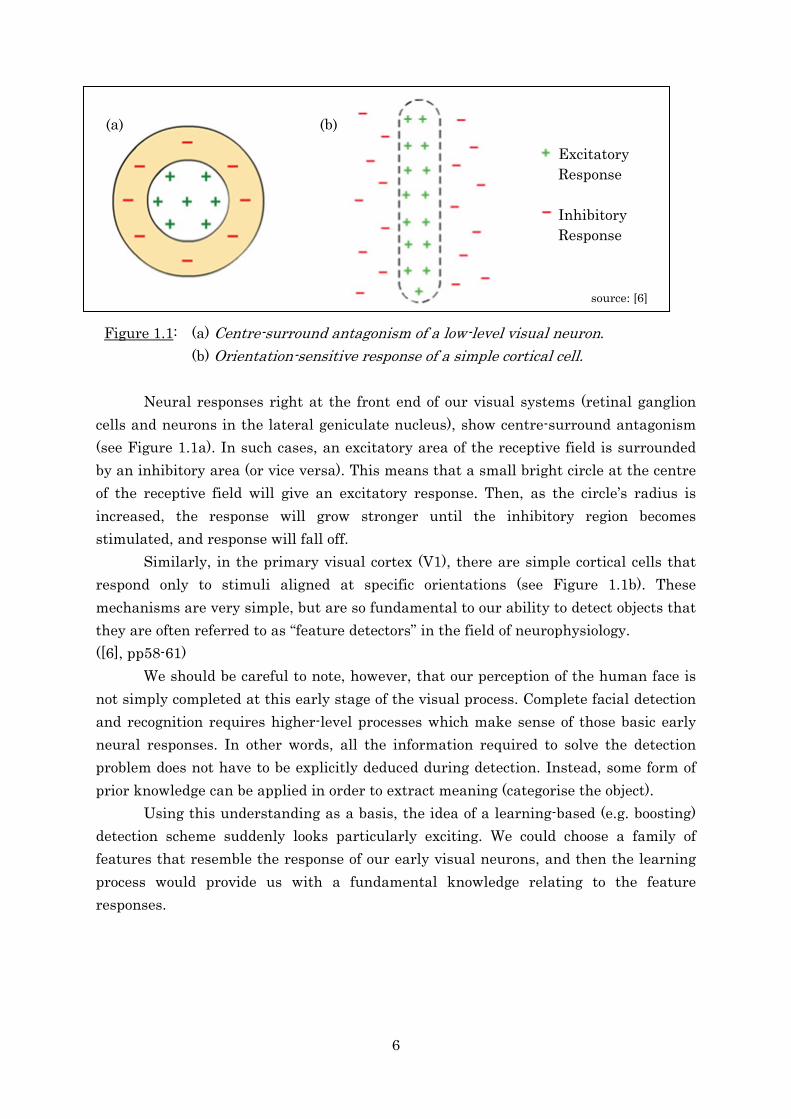
Figure 1.1: (a) Centre-surround antagonism of a low-level visual neuron.

(b) Orientation-sensitive response of a simple cortical cell.

Neural responses right at the front end of our visual systems (retinal ganglion

cells and neurons in the lateral geniculate nucleus), show centre-surround antagonism

(see Figure 1.1a). In such cases, an excitatory area of the receptive field is surrounded

by an inhibitory area (or vice versa). This means that a small bright circle at the centre

of the receptive field will give an excitatory response. Then, as the circle’s radius is

increased, the response will grow stronger until the inhibitory region becomes

stimulated, and response will fall off.

Similarly, in the primary visual cortex (V1), there are simple cortical cells that

respond only to stimuli aligned at specific orientations (see Figure 1.1b). These

mechanisms are very simple, but are so fundamental to our ability to detect objects that

they are often referred to as “feature detectors” in the field of neurophysiology.

([6], pp58-61)

We should be careful to note, however, that our perception of the human face is

not simply completed at this early stage of the visual process. Complete facial detection

and recognition requires higher-level processes which make sense of those basic early

neural responses. In other words, all the information required to solve the detection

problem does not have to be explicitly deduced during detection. Instead, some form of

prior knowledge can be applied in order to extract meaning (categorise the object).

Using this understanding as a basis, the idea of a learning-based (e.g. boosting)

detection scheme suddenly looks particularly exciting. We could choose a family of

features that resemble the response of our early visual neurons, and then the learning

process would provide us with a fundamental knowledge relating to the feature

responses.

source: [6]

(a) (b)

Excitatory

Response

Inhibitory

Response

7

Chapter 2

Technical Framework

2.1 Review of Colour-based Feature Point Detection

2.1.1 Research Context (information for Imperial College markers)

The facial expression recognition system of [23] had been developed in the Social

Robotics research lab at National University of Singapore. I was provided with the

related C++ code project. None of this code was used in the final implementation, but it

provided useful learning material. It comprised around 5000 lines, which included large

sections unrelated to feature point detection. I was asked to address three main issues:

• The feature point detection system was somewhat unreliable. In particular, it

was very sensitive to changes in pose. It was hoped that minor modifications of

this method would lead to acceptable performance.

• The code worked in isolation, but needed to be incorporated into the lab’s overall

robot vision framework in order to be compatible with the other vision components

being developed in the lab.

• The code made use of several non-standard libraries. The lab requires that only

OpenCV 1.0 and wxWidgets libraries can be used in addition to the standard

libraries. OpenCV is an open source computer vision library, originally developed

by Intel. Full details can be found here: [38].

This represented some months of work and provided significant insight into the

problem at hand, so will be summarised here.

Despite our strong arguments supporting a learning-based feature point

detection method, a colour-based approach was not necessarily a bad way to start. This

method is intuitive and conceptually simple, and as such provided an insightful

introduction to detection, programming with OpenCV and object-oriented programming

in general.

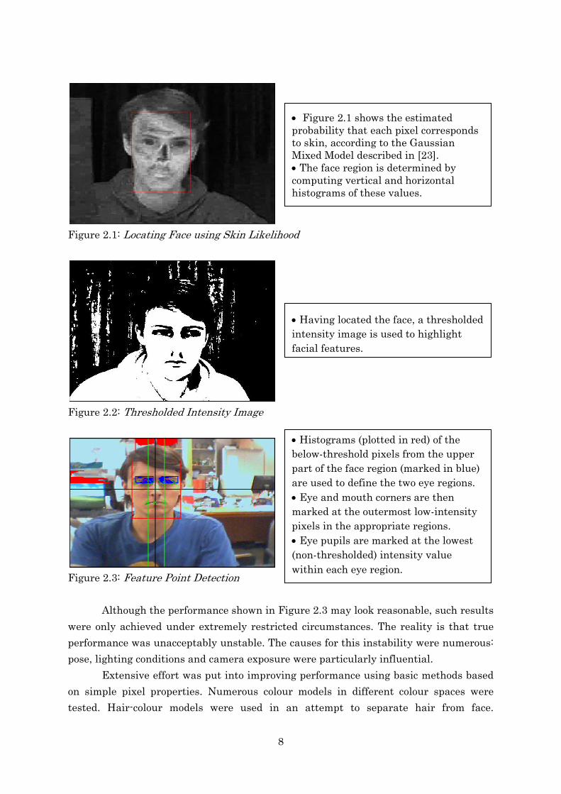
The detection algorithm, based on [23], is summarised as follows:

8

Figure 2.1: Locating Face using Skin Likelihood

Figure 2.2: Thresholded Intensity Image

Figure 2.3: Feature Point Detection

Although the performance shown in Figure 2.3 may look reasonable, such results

were only achieved under extremely restricted circumstances. The reality is that true

performance was unacceptably unstable. The causes for this instability were numerous:

pose, lighting conditions and camera exposure were particularly influential.

Extensive effort was put into improving performance using basic methods based

on simple pixel properties. Numerous colour models in different colour spaces were

tested. Hair-colour models were used in an attempt to separate hair from face.

• Figure 2.1 shows the estimated

probability that each pixel corresponds

to skin, according to the Gaussian

Mixed Model described in [23].

• The face region is determined by

computing vertical and horizontal

histograms of these values.

• Having located the face, a thresholded

intensity image is used to highlight

facial features.

• Histograms (plotted in red) of the

below-threshold pixels from the upper

part of the face region (marked in blue)

are used to define the two eye regions.

• Eye and mouth corners are then

marked at the outermost low-intensity

pixels in the appropriate regions.

• Eye pupils are marked at the lowest

(non-thresholded) intensity value

within each eye region.

9

Morphological ‘opening’ was used to separate eyebrows from eyes. ‘Closing’ and

connectivity-based segmentation were used in an attempt to classify which feature a

pixel belonged to.

In summary, we feel that this task was made particularly difficult by the fact

that there was not a single reliable reference. Face height is difficult to define due to

variability in fringe hair and exposed neck skin. Determining face width is equally

problematic – no single skin-likelihood threshold could consistently separate skin from

background objects. This was caused not only by ambient lighting, but also pose relative

to the light source. Despite skin being largely homogeneous, the non-planar shape of our

faces can give rise to significant variation in the light received by the camera, even

within a single frame. It did not seem that any non-adaptive skin colour model could

adequately cope with this while, at the same time, non-skin (background) pixels were

also regularly misclassified.

The reliability of the face region is fundamental to the success of this approach.

Subsequent detection stages rely heavily on facial dimensions in order to define their

search regions. Even when these regions are well-defined, this method faces the same

problems when refining the search towards feature points.

Intuitively, the problem seemed quite simple, but selecting effective parameters

proved to be unbelievably difficult in practice.

2.1.2 Relating Back to the Human Visual System

An interesting lesson we can take from this is that our own visual systems can

perhaps deceive us into believing that aspects of this detection task are straightforward.

Our vision continuously adapts incredibly seamlessly to a wide range of variations.

Thus, it becomes difficult for us to obtain an objective and accurate view of what the

true nature of the visual stimulus really is. So, perhaps surprisingly, our ability to solve

this problem through conscious reasoning seems to be heavily restricted by the

immensely powerful subconscious mechanisms that do the job for us.

This really outlines the need for a greater level of abstraction. This is why we

need to embed our images in a high-dimensional feature space, and this is why we will

finally reject this method.

10

2.2 A Learning-based Approach

We have already discussed several points that make a learning-based detection

system a particularly exciting option. For us, there are two approaches that seem to

really stand out in addressing all our requirements. These methods are somewhat

similar in that they are both adaptations of the ground-breaking Viola-Jones algorithm

[25].

So, a strong understanding of the Viola-Jones algorithm is required before we can

go on to choosing and fully understanding an eventual method.

2.2.1 The Viola-Jones Algorithm

In short, the Viola-Jones method achieves detection at very high speed and has

been shown to perform well in detecting various objects, such as faces [25], facial

features [32] and pedestrians [26]. There seems to have been little interest in applying

this method to feature point detection, but we will see that there is significant potential

if the correct restrictions are applied.

There were three really major contributions given by the Viola-Jones method: the

“integral image” representation, a modified version of AdaBoost boosting algorithm and

a cascaded classifier architecture.

(i) Integral Image

An integral image is an alternative representation of the standard greyscale

image. The point (x,y) in the integral image is simply given by the sum of all points

above and to the left of this point in the greyscale image:

' , '

( , ) ( ', ')x x y y

ii x y i x y< <

= ∑

where ii(x,y) is the integral image and i(x’,y’) is the original image.

The motivation for doing this conversion is that it allows the pixel sum of any

rectangular image region to be computed using just four array references (one at each

corner). This is immensely efficient and is calculated in constant time regardless of

region size.

Viola-Jones then takes advantage of this efficient representation by defining a

set of features that are made up of rectangular regions. Some examples of these so-

called “Haar-like” features are shown below:

11

Figure 2.4: Various Haar-like features within a fixed-size detection window.

The value of a feature is given by the summed difference between the black and

white rectangular regions. It is very important to note that the feature is not just

defined by the Haar-like shape alone. Whilst we generally use the word ‘feature’ to refer

to just the Haar-like basis function, strictly speaking, scale and location within the

detection window are equally important. So, in order to resolve any potential ambiguity,

we will state the full 5-dimensional representation of a feature:

- Feature TypeFeature TypeFeature TypeFeature Type – this describes the layout of the chosen Haar-like basis function.

The Viola-Jones method uses 3 main categories of feature types: two-, three- and

four-rectangle (see Figure 2.4).

- (x,y)(x,y)(x,y)(x,y) – exact location (coordinate) corresponding to feature response.

- (width,height)(width,height)(width,height)(width,height) – describes the scale of the Haar-like basis function. This should

not be confused with the detection window size, which is fixed relative to the

Haar-like kernel.

With multiple feature types, scales and translations, the total number of features

for a given region will obviously be large. In fact, the number is much larger than the

total number of pixels within the detection window. For example, a 24x24 (576-pixel)

detection window supports 45,396 Haar-like features. Of course we now need some

method of reducing dimensionality in order to select only a small number of features

that give the best classification performance.

(ii) AdaBoost

We introduced the topic of boosting as a method of dimensionality reduction in

the ‘Background’ section. It is now necessary to understand in explicit detail how this

algorithm combines results from a simple learning algorithm (weak learner) to form a

strong classifier. There is a certain amount of vocabulary we need to familiarise

ourselves with, so we will start with a formal definition then work towards a more

intuitive understanding.

12

A formal explanation of the full algorithm [25] is given as follows:

Here, the number of weak classifiers that combine to form a strong classifier is

given by T. We will look at how this value is determined when we later discuss the

detector cascade.

Another very important point we must highlight is the subtle difference between

a feature and a weak classifier (see part (2) of the algorithm). Although we often discuss

features and weak classifiers analogously, strictly speaking, a weak classifier is actually

what we get as a result of training with a single feature. To clarify, a weak classifier is

therefore dependent on feature, threshold and parity:

• Given example images ( ) ( ), , ... , , i i n nx y x y where 0,iy 1= for negative and

positive examples respectively.

• Initialize weights 1, 1/ 2 ,1/ 2 iw m l= for 0,iy 1= respectively, where m and l are

the number of negatives and positives respectively.

• For 1,...,t T= :

1) Normalise the weights,

,

,

,1

t i

t i n

t jj

ww

w=

←∑

so that tw is a probability distribution.

2) For each feature, j , train a classifier jh which is restricted to using a single

feature. The error is evaluated with respect to , ( )t j i j i iiw w h x yε = −∑ .

3) Choose the classifier, th , with the lowest error tε .

4) Update the weights:1

1, , ie

t i t i tw w β −+ =

where 0ie = if example ix is classified correctly, 1ie = otherwise and 1

tt

t

εβ

ε=

−

• The final strong classifier is:

1 1

11 ( )

( ) 2

0 otherwise

T T

t t tt th x

h xα α

= =

≥=

∑ ∑

where 1

logt

t

αβ

=

13

- Feature Feature Feature Feature – the 5-dimensional entity we defined above.

- thresholdthresholdthresholdthreshold – determined by the weak learner (to minimise misclassifications).

- parityparityparityparity – describes whether we subtract the white rectangle pixel sum from the

black rectangle pixel sum or vice versa.

Having gained all of the necessary vocabulary and resolved any ambiguities, we

should now be able to summarise Viola-Jones’ adapted AdaBoost algorithm with total

clarity:

Since weights are reallocated every time a weak classifier is selected, all weak

classifiers must be completely learnt from scratch on each iteration. As we have

discussed, the set of features is quite large. The sets of positive and negative samples

will also generally number in the thousands. So, even with the great efficiency of the

integral image representation, this process requires a very large amount of computation.

Obviously, the number of features to be used for detection is only a relatively tiny

subset of those used in training. However, with computational efficiency being so

important, Viola-Jones also offers the following cascaded structure to greatly reduce the

number of classifiers used during detection.

(iii) Detection Cascades

The key to the success of the cascade detector structure essentially rests on the

following statement:

It is much easier to say for sure that a given detection region definitely does notnotnotnot contain

a positive match, than it is to be sure that it definitely doesdoesdoesdoes.

• Initially, all sample weights are fairly distributed.

i. The weak learner takes a single feature and forms a weak classifier by setting a

threshold and parity that best classifies the samples. This is repeated for all

features.

ii. The lowest-error weak classifier is selected and applied to the samples.

iii. The weights of the samples are then reallocated to emphasise those that were

misclassified.

• Stages (i) – (iii) are repeated T times.

• The strong classifier is formed by a weighted linear combination of the T weak

classifiers, with a threshold that yields low error-rate.

14

So, if we can quickly discard those ‘easy’ negative matches, more sophisticated detection

only needs to be carried out in the more promising image regions.

The cascade does this by performing detection in stages, each one a different

strong classifier. The early stages use simple, computationally efficient features to

achieve high-speed rejection. The latter stages then use more complex features in order

to resolve the more difficult regions and reduce false positive rates.

The idea is that while a positive match will have to pass through every detection

stage, this is an extremely rare occurrence. The vast majority of detection regions are

rejected at an early stage.

Figure 2.5: Schematic of an N-stage Detection Cascade.

Since the false positive rate (‘false alarm rate’) and successful detection rate (‘hit

rate’) both progress multiplicatively, the classifier thresholds need to be kept low in

order to minimise false negatives. What we are now saying is that the objective is no

longer to maximise classification with every classifier (as was the case with our original

discussion of AdaBoost). The important thing now is that we don’t discard any positive

matches whilst we quickly reject definite negatives. So the threshold for selecting a

strong classifier (initially set at1

T

ttα

=∑ ) needs to adapt to accommodate this.

The way this is done is to enforce limits on the minimum hit rate and maximum

false alarm rate for each cascade stage during training. For example, we may require a

minimum hit rate of 0.995 and a maximum false alarm rate of 0.5. For a 15-stage

classifier cascade, the worst-case result would then be an overall false detection rate of

0. 015 55 3x1 −≈ , whilst still maintaining an overall hit rate of 0.99 0.93155 ≈ .

In order to accommodate these constraints, the number of weak classifiers per

strong classifier, T, has to be allowed to vary. For example, higher maximum hit rates

and lower minimum false alarm rates will generally require a larger number of weak

classifiers in order to meet these tight constraints. This would, in theory, allow better

classification performance per cascade stage, but the trade-off is that this will also

increase computation at each stage.

All

Sub-windows

Rejected Sub-windows

1 2 3 Positive

Match N

15

However, we should be mindful of the fact that peak classification performance

will ultimately depend on the quality and quantity of our training data. An infinite

number of ‘perfect’ samples does not exist. So, in using looser detection requirements to

speed up detection, the actual sacrifice in classification performance may be relatively

small.

2.2.2 Adaptations of Viola-Jones

Now that we have a strong understanding of the Viola-Jones algorithm, we can

finally move on to look briefly at the adaptations of this method. The first one we will

consider was proposed by Lienhart et al. [27]. The biggest contribution of this paper was

to extend the Haar-like feature set, but it also presented analysis of alternative boosting

algorithms.

The major change to the feature set was the inclusion of rotated features. The

integral image offered by Viola and Jones only allowed for the fast computation of

upright rectangular image areas. So, Lienhart et al. use a second auxiliary image (the

Rotated Summed Area Table, RSAT) to achieve fast computation of rectangles offset by

an angle of 45° to the horizontal. The details of how the RSAT can be computed in a

single pass over the image can be found in [27].

There are also some adapted line features and, interestingly, centre-surround

features:

Figure 2.6: The extended Haar-like feature set proposed in [27].

Now a fascinating observation is to compare these features with the neural

responses we saw earlier in Figure 1.1. The similarities are striking, but in using

computationally-efficient rectangular shapes, the Haar-like features are relatively

‘blocky’ and imprecise in nature.

It is generally accepted that the best way of modelling those neural responses is

actually to use Gabor filters [28, 29]. This brings us on to our discussion of the approach

4. Diagonal Line Feature 2. Line Features

3. Centre-surround Features 1. Edge Features

16

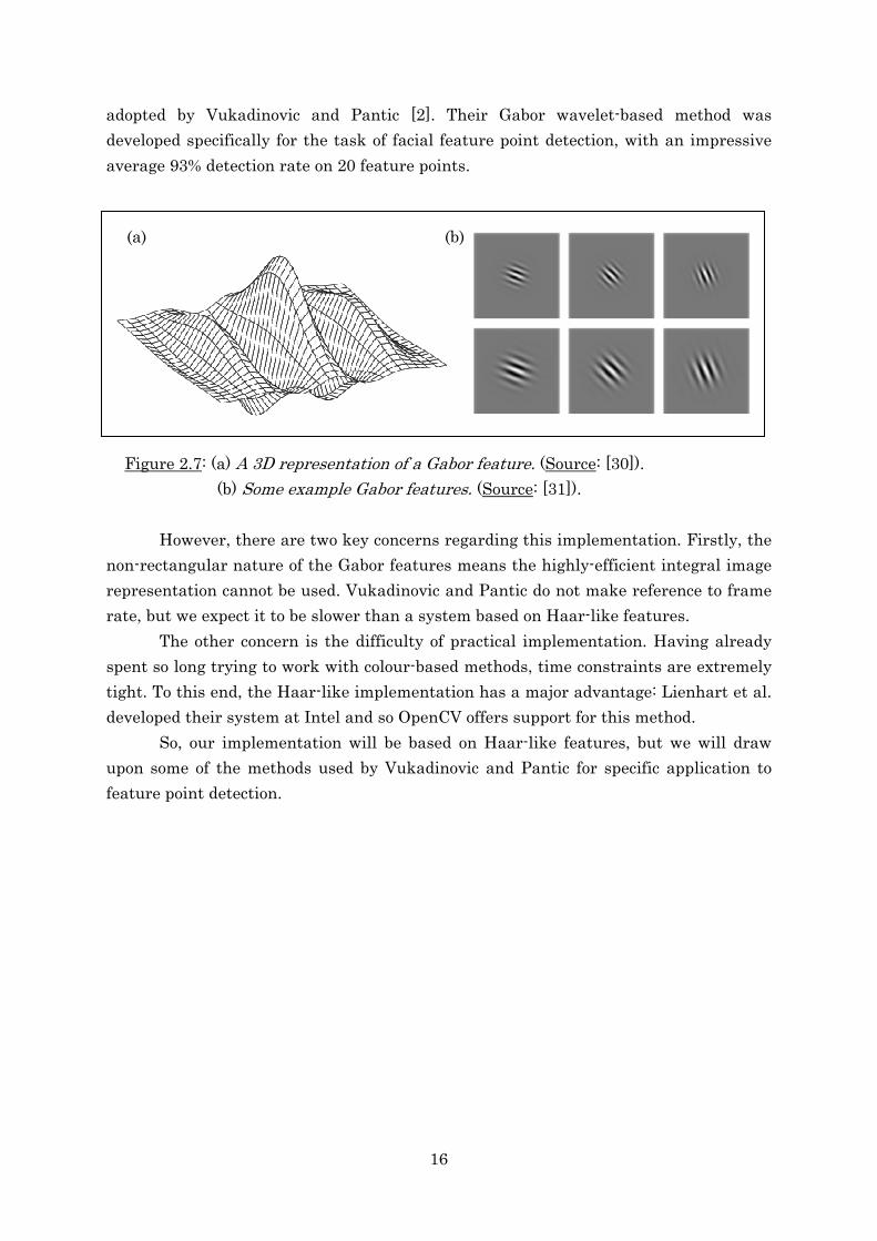
adopted by Vukadinovic and Pantic [2]. Their Gabor wavelet-based method was

developed specifically for the task of facial feature point detection, with an impressive

average 93% detection rate on 20 feature points.

Figure 2.7: (a) A 3D representation of a Gabor feature. (Source: [30]).

(b) Some example Gabor features. (Source: [31]).

However, there are two key concerns regarding this implementation. Firstly, the

non-rectangular nature of the Gabor features means the highly-efficient integral image

representation cannot be used. Vukadinovic and Pantic do not make reference to frame

rate, but we expect it to be slower than a system based on Haar-like features.

The other concern is the difficulty of practical implementation. Having already

spent so long trying to work with colour-based methods, time constraints are extremely

tight. To this end, the Haar-like implementation has a major advantage: Lienhart et al.

developed their system at Intel and so OpenCV offers support for this method.

So, our implementation will be based on Haar-like features, but we will draw

upon some of the methods used by Vukadinovic and Pantic for specific application to

feature point detection.

(a) (b)

17

Chapter 3

Implementation

Constructing our detector requires two main stages: training then detection.

Despite this chronological order, decisions regarding training affect the detector and vice

versa. Therefore we will divide our description of the detector so that some aspects can

be discussed after we have some understanding of training techniques.

A lot of effort was put into making it quick and easy to add any new detectors to

the system. A separate document has been prepared detailing the simple practical steps

required to do this – from training to detection (see Appendix A).

3.1 Detector Structure

The key to our method rests on the fact that, although facial feature points

contain considerably less structural information than a whole face, the background in

which we find them is also very restricted. In other words, if we can reliably narrow the

search area down to a relatively small region around the feature point, then our task is

made much easier.

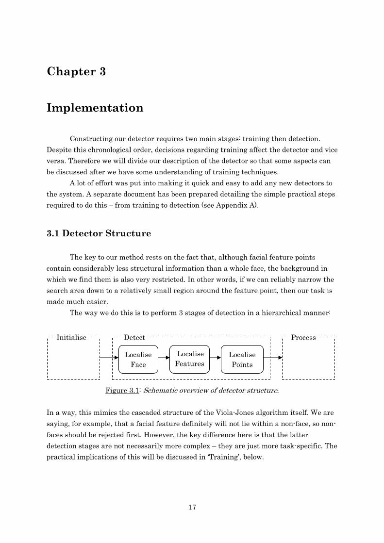
The way we do this is to perform 3 stages of detection in a hierarchical manner:

Figure 3.1: Schematic overview of detector structure.

In a way, this mimics the cascaded structure of the Viola-Jones algorithm itself. We are

saying, for example, that a facial feature definitely will not lie within a non-face, so non-

faces should be rejected first. However, the key difference here is that the latter

detection stages are not necessarily more complex – they are just more task-specific. The

practical implications of this will be discussed in ‘Training’, below.

Initialise Detect

Localise

Face

Localise

Features

Localise

Points

Process

18

3.2 Design Considerations

A desirable property of many computer vision systems is rotation-scale-

translation (RST) invariance. Our detector is no different – we wish for detection to be

achieved regardless of how the face is located, scaled or orientated within the image.

The Viola-Jones method can achieve translation and (most) scale invariance due

to the way the whole image is searched at numerous scales. A degree of lighting

correction is also achieved through contrast stretching [27]. Rotation invariance is not

intrinsically possible, but due to the specific nature of our problem, we can seek to partly

address this issue.

In a 3D vision problem, we are concerned with rotation about the three spatial

axes:

Figure 3.2: Rotation about (a) x-axis (b) y-axis and (c) z-axis.

Under normal circumstances, facial rotations about the x-axis don’t exceed

relatively small nodding motions. Rotation about the y-axis is much more problematic,

since the 3D shape of the face is such that this rotation can lead to features being

occluded from view. As such, we will leave these for discussion in the “Future Work”

section.

However, the problem we can seem to address is rotation about the z-axis

(rotations parallel to the image plane). This problem should be relatively easy to solve,

since the information available in the image is effectively not changed. All we need to do

is detect this rotation, and then we should be able to retrieve facial information in the

same way as for an upright face.

We propose to track this rotation about the z-axis by using our detected feature

points to provide a reference. In particular, eye corners are distributed in a somewhat

horizontal manner across the face and remain relatively fixed under changing facial

expression. Thus, by estimating a best-fit line that connects these points, we can

compute its angle offset to the horizontal and correct our system accordingly.

Since we are only trying to detect a single line, a basic linear least squares (LLS)

approach should be sufficient. We construct the LLS problem by simply rearranging the

equation of a straight line into the required form Axxxx = b:

(a) (b) (c)

19

The next step is to compute the singular value decomposition (SVD) of the matrix

A, to give A = UDVT. The least squares solution for xxxx is then given by xxxx = A+b, where A+

is the pseudoinverse of A and is given by:

(where D0 is the diagonal matrix of the singular values of A).

Having obtained xxxx = [-m/c, 1/c]T, a simple rearrangement yields the gradient of

the best fit line, m. Finally, the estimated facial tilt offset angle is given by α = tan-1(m).

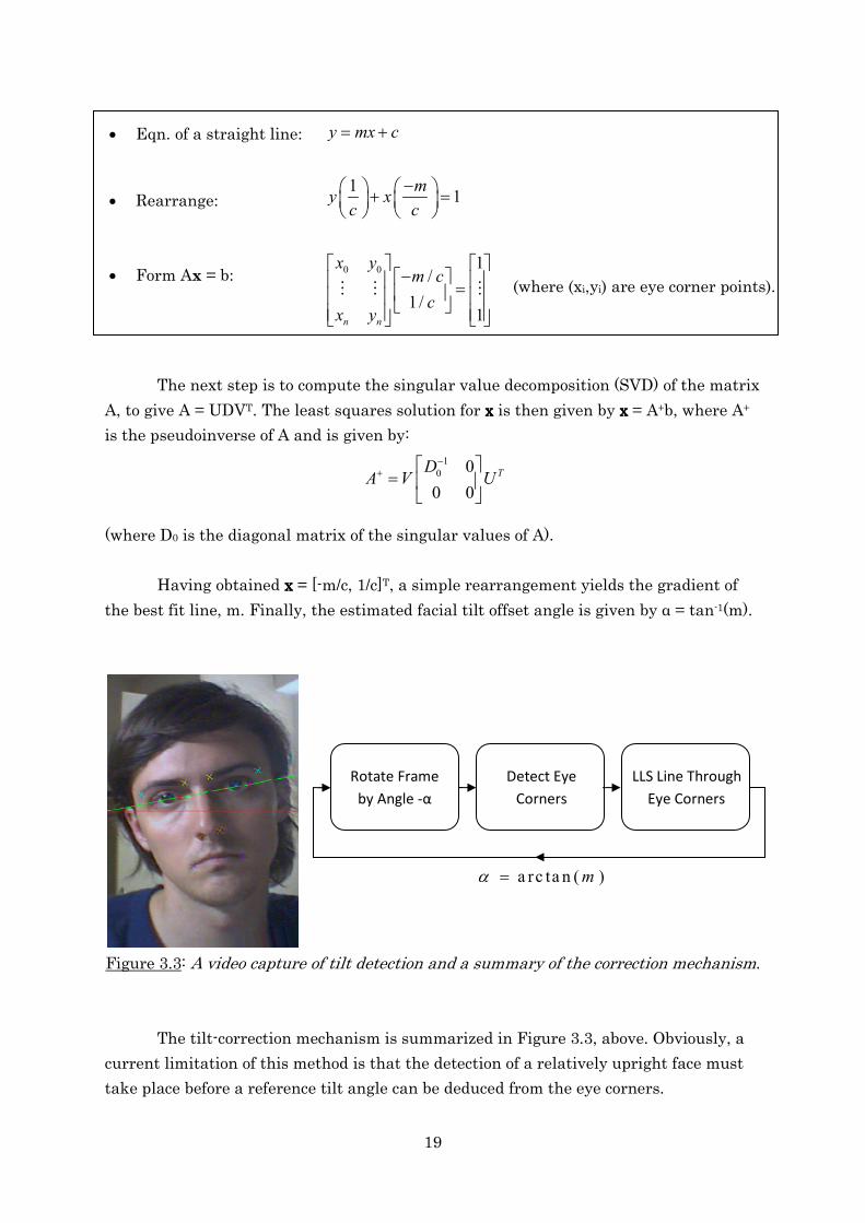
Figure 3.3: A video capture of tilt detection and a summary of the correction mechanism.

The tilt-correction mechanism is summarized in Figure 3.3, above. Obviously, a

current limitation of this method is that the detection of a relatively upright face must

take place before a reference tilt angle can be deduced from the eye corners.

1

0 0

0 0

TDA V U

−+ =

LLS Line Through

Eye Corners

Detect Eye

Corners

Rotate Frame

by Angle -α

a rc ta n ( )mα =

• Eqn. of a straight line:

• Rearrange:

• Form Ax = b: (where (xi,yi) are eye corner points).

0 0

11

1/

1/1n n

y mx c

my xc c

x ym c

cx y

= +

− + =

− =

⋮ ⋮ ⋮

20

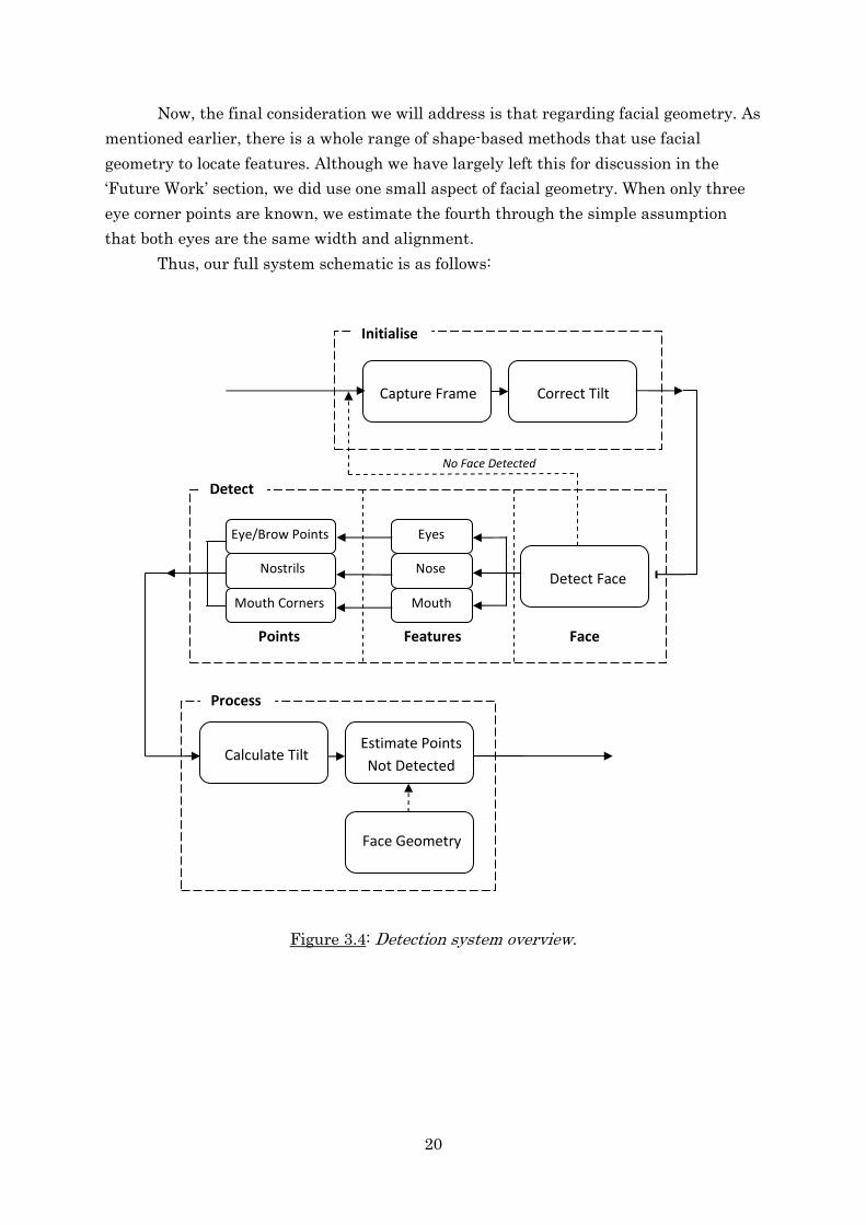
Now, the final consideration we will address is that regarding facial geometry. As

mentioned earlier, there is a whole range of shape-based methods that use facial

geometry to locate features. Although we have largely left this for discussion in the

‘Future Work’ section, we did use one small aspect of facial geometry. When only three

eye corner points are known, we estimate the fourth through the simple assumption

that both eyes are the same width and alignment.

Thus, our full system schematic is as follows:

Figure 3.4: Detection system overview.

No Face Detected

Capture Frame Correct Tilt

Initialise

Calculate Tilt Estimate Points

Not Detected

Face Geometry

Process

Detect

Face Points Features

Detect Face Nose

Mouth

Eyes Eye/Brow Points

Nostrils

Mouth Corners

21

3.3 Training

We will now discuss how detection cascades were trained for feature points. In

order to concentrate fully on the task of feature point detection, we chose not to train our

own face or feature detectors (since samples of these are available in the public domain).

The face detector we used was OpenCV’s “haarcascade_frontalface_alt2.xml”. Detectors

for Left Eye, Right Eye, Nose and Mouth, were obtained from [32].

3.3.1 Image Database

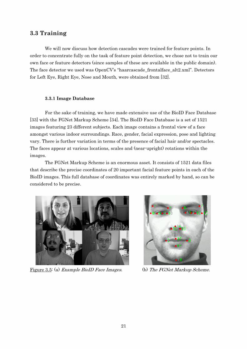
For the sake of training, we have made extensive use of the BioID Face Database

[33] with the FGNet Markup Scheme [34]. The BioID Face Database is a set of 1521

images featuring 23 different subjects. Each image contains a frontal view of a face

amongst various indoor surroundings. Race, gender, facial expression, pose and lighting

vary. There is further variation in terms of the presence of facial hair and/or spectacles.

The faces appear at various locations, scales and (near-upright) rotations within the

images.

The FGNet Markup Scheme is an enormous asset. It consists of 1521 data files

that describe the precise coordinates of 20 important facial feature points in each of the

BioID images. This full database of coordinates was entirely marked by hand, so can be

considered to be precise.

Figure 3.5: (a) Example BioID Face Images. (b) The FGNet Markup Scheme.

22

3.3.2 Positive Samples

In our overview of eigenfaces (in ‘Background’), we briefly mentioned the

importance of equal scale, alignment and rotation of positive training images. Features

in the Viola-Jones method are also defined according to their spatial location, so the

same principles apply. What we want is for the salient information (which defines the

feature point) to be distributed equally in each sample and so Haar-like features stand a

better chance of returning similar responses to all positive samples.

During training, the issue of correctly centring the sample is achieved by use of

the provided coordinate ground truths. The Viola-Jones method is also intrinsically

resistant to variation in ambient light intensity. However, we still have to look at ways

to correct tilt and normalise scale. It should be noted that we only do this during the

creation of positive samples, since a greater degree of generality is desirable in negative

samples. This ensures better rejection of false positive classifications at an early stage.

(i) Correcting Sample Tilt

We have already discussed the idea of correcting facial tilt during detection.

Applying the same process to our database of face images should align the samples as

desired.

In our earlier discussion of tilt-correction during detection, the image rotation

was achieved using OpenCV functions. However, we now need to rotate our ground

truth coordinate values explicitly, so we will discuss a method for doing this [35].

We consider representing a point, P, in x-y and the rotated coordinate space, x’-y’:

Figure 3.6: Rotating the coordinate axes.

x’

y’

y

x

P

θ

α

O

cos( )

sin( )

' cos( )

' sin( )

x OP

y OP

x OP

y OP

θ αθ α

θθ

= +

= +

=

=

23

We can now express the x-y coordinates in terms of the x’-y’ coordinates by using

the standard trigonometric angle sum relations:

sin( ) sin( ) cos( ) cos( ) sin( )

cos( ) cos( ) cos( ) sin( )sin( )

a b a b a b

a b a b a b

+ = +

+ = −

This yields:

The centre of this rotation is somewhat arbitrary for our purposes. We choose the

image centre, since this means the image data that we inevitably discard during a

rotation is evenly distributed and minimal. We incorporate this correction term into the

above equations to finally yield:

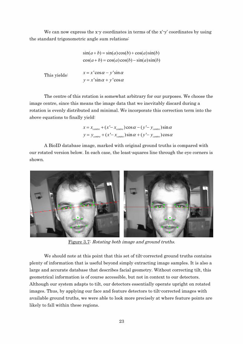
A BioID database image, marked with original ground truths is compared with

our rotated version below. In each case, the least-squares line through the eye corners is

shown.

Figure 3.7: Rotating both image and ground truths.

We should note at this point that this set of tilt-corrected ground truths contains

plenty of information that is useful beyond simply extracting image samples. It is also a

large and accurate database that describes facial geometry. Without correcting tilt, this

geometrical information is of course accessible, but not in context to our detectors.

Although our system adapts to tilt, our detectors essentially operate upright on rotated

images. Thus, by applying our face and feature detectors to tilt-corrected images with

available ground truths, we were able to look more precisely at where feature points are

likely to fall within these regions.

'cos 'sin

'sin 'cos

x x y

y x y

α αα α

= −

= +

( ' ) cos ( ' )sin

( ' ) sin ( ' ) cos

centre centre centre

centre centre centre

x x x x y y

y y x x y y

α α

α α

= + − − −

= + − + −

24

(ii) Normalising Scale

In order to normalise sample scales, we need some sort of reference measure that

is relatively consistent in all face images. A further consideration is that of local scale; if

the face does not lie parallel to the image plane, then features across different depths

(within the same face) will appear at inconsistent scales.

For these reasons, we choose our reference to be eye width (magnitude of the

distance between inner and outer eye corners). Compared to mouth and brows, eyes stay

relatively stationary under varying expression. They are situated at each side of the

face, so should give good scale reference on that side.

Next, we have to decide on the approximate amount of facial information we

want in each sample. There does not seem to be any definite way to make this decision.

Indeed, no publications we found seemed to normalise scale at all. So, we chose to centre

our scales around the fixed size proposed by Vukadinovic and Pantic: 13x13.

So, we initially propose to select sample size is as follows:

1. Find the mean magnitude of relevant eye width for all images in database.

2. Rescale these values such that mean = 13.

3. Round to nearest odd integer (to allow a well-defined centre pixel).

This gave us various sample sizes ranging from 7x7 to 33x33. This great variation would

seem to illustrate the importance of scale normalisation.

In terms of the information each sample contains, for example, for the inner

corner of the left eye, every positive image reached from the extremity of the canthus to

the edge of the pupil.

However, in practice, this approach was found to give surprisingly poor results. It

seems that applying such a tight restriction on scale makes it difficult to pinpoint the

correct scale during detection. The way we addressed this problem was to instead use a

small range of image patch sizes for each feature point, then rescale them all to the

correct normalised scale. After some trial and error, we decided to have two additional

scales – one smaller and one larger (to the nearest odd number):

Figure 3.8: Samples at 3 scales for (a) Nostril and (b) Outer Left Brow.

This seemed to give the greater generality that we needed, without any

significant increase in false positives.

(a) (b)

25

(iii) Horizontal Mirroring

The human face displays a degree of horizontal symmetry and this should be

exploited. So, instead of training a feature point detector for every facial feature point,

we only did so for left-side feature points. Then, during detection, the right-side regions

of interest were flipped for detection, and then the detected point could be flipped back.

We should note that flipping image patches during detection may slow detection

down. However, the image patches are small and the many days of training computation

saved were believed to be more significant. A long-term solution to this problem would

be to alter the detection cascade xml files directly. This will be discussed later in ‘Future

Work’.

Of course, our faces are not perfectly symmetrical, so we could also double the

size of our training databases by flipping sample image patches from the right side of

the face. However, in practice, we found that this offered no significant increase in

performance. This makes sense because the variation of a given feature between the left

and right sides of a single face are likely to be tiny compared to the difference between

two different people.

One variation that may be offered by left-right sample pairs is that of scale. Any

face that is not perfectly frontally-facing will have left and right features at different

depths (and therefore different scales). However, we feel that our systematic method of

normalising scale in proportion to local feature dimensions and then rescaling explicitly

is far more adaptable and rigorous.

3.3.3 Negative Samples

As previously mentioned, the background information local to each feature point

is very restricted in nature. This is a very powerful statement. In contrast to most

standard detection tasks, it is not necessary for us to achieve detection amongst

massively varying backgrounds (such as indoor and outdoor scenes). Instead, we just

have to deal with the relatively homogenous set of local skin regions.

In order to do this, we have adapted the method used by Vukadinovic and Pantic.

In their work, they proposed that 9 positive and 16 negative samples (sized 13x13

pixels) could be taken for each feature point:

26

Figure 3.9: Positive and negative sample selection method, used in [2].

Their positive samples are in a 3x3 block, centred on the feature point. Then,

there are 8 inner and 8 outer negative samples. The inner samples are randomly located

at a 2-pixel distance from the positive sample block. The outer samples are randomly

distributed in a local region (which we set to be one eye width squared).

The only difference with our method is that we only have one positive sample per

image feature. We felt that, after incorporating our method of multiple scaling, we were

able to achieve some spatial variation, while using 3 samples rather than 9 (therefore

allowing faster training). Note that scale normalisation and tilt correction were only

carried out on positive samples, since negative patches need to be rejected at all scales

and rotations.

3.4 C++ Code Implementation

Please refer to Appendix A for full details on how a detector can be implemented.

In summary, any feature or feature point can be passed into the same detection function

by simply initialising its following members:

CvRect ROI; //general ROI for detection double HaarParams[4]; //Viola-Jones detection parameters CvHaarClassifierCascade* cascade; //Haar cascade xml file bool IsPoint; //for face, eyes etc: want LARGEST region, not point bool OK; //check if feature found bool OnRightSide; //flip image patches for right-side features

27

Chapter 4

Results

4.1 Testing Datasets

In order to carry out thorough quantitative analysis of our system, it would be

desirable to perform detection on a marked face database, like the BioID Database. That

way, we could make accurate comparisons between ground truths and our estimated

feature point locations. However, we cannot use our training database for testing as this

will not give us any idea of generalisation.

One could argue that the right-side feature points were not used in training and

therefore could be used for testing purposes. However, as we said before, variations

between the two sides of a single face are relatively small. Instead, we really need to see

if our training database has provided enough generality to perform well on any face.

An alternative approach could have been to reserve a subset of the BioID

Database just for testing. However, this would have left fewer images available for

training and so detection performance may have suffered. Also, with only 23 different

subjects in the database, there is not much scope to train and test on different people.

Unfortunately, the only other (free) marked-up database we could find contained

just one face. Thus, our testing comprises two main parts:

i) Quantitative evaluation using a marked-up database of just one face.

ii) Qualitative analysis using a database containing many different subjects.

The marked-up database we used is the “Talking Face Video” from FGNet [36]. It

comprises a sequence of 5000 frames showing a person in conversation. There are 68

points marked on each frame (these include all the points we detected). We used the

first 2000 frames.

Our second test database is the Facial Recognition Technology (FERET) colour

database [37]. Unfortunately, the FERET database includes many non-frontal images

(such as left and right profile views), which are not relevant to our work. So, we first had

to segment the database and extract only the frontal images. We used 1175 images from

DVD 1 of the FERET Database.

Please Note: Due to the large number of images involved, only a few results can

be shown in this report. The full results, along with further real-time detection results,

can be viewed in video form at: YouTube.com/HarryComminFYPYouTube.com/HarryComminFYPYouTube.com/HarryComminFYPYouTube.com/HarryComminFYP

28

4.2 Results from Marked-up Database

Since this database is effectively a video sequence, we can incorporate facial tilt

correction between frames. We will therefore measure the effectiveness of facial tilt

correction by comparing detection scores with and without tilt correction.

One way of classifying a successful detection is by measuring proximity to ground

truth value as a proportion of inter-ocular distance (distance between eye centres). In

agreement with Vukadinovic and Pantic, we believe that 30% of inter-ocular distance is

far too approximate and that 10% is a more meaningful measure.

Figure 4.1: The allowable margin of error for ‘success’ (10% of inter-ocular distance).

According to this definition of ‘success’, we achieved the following results:

Feature Point No Tilt

Correction

Full Tilt

Correction

Half Tilt

Correction

Inner Left Brow

78.65% 93.10% 96.40%

Outer 99.05% 95.30% 97.95%

Inner Right Brow

99.50% 96.85% 99.90%

Outer 99.30% 69.65% 66.90%

Outer

Left Eye

94.35% 95.20% 98.20%

Pupil 92.00% 92.75% 94.80%

Inner 96.05% 94.45% 97.45%

Inner

Right Eye

98.15% 95.30% 98.20%

Pupil 92.50% 92.05% 94.60%

Outer 96.35% 95.00% 97.35%

Left Nostrils

98.05% 94.80% 97.45%

Right 98.80% 96.25% 98.85%

Left Mouth

83.00% 86.55% 89.60%

Right 81.85% 86.50% 89.85%

93.40% 91.70% 94.11%

Figure 4.2: Success rates for each feature point.

29

Overall, results are encouraging. The system largely succeeded above 90% for

most feature points. As we would expect, performance regarding mouth corners was

below average. This is very much a topic for future development (see Future Work,

below).

The performance when using tilt correction was perhaps a little disappointing. It

was initially thought that this could be due to unwanted fluctuations in tilt estimation.

So, we tried reducing this by only partly correcting tilt (by half). Further investigation is

required to see whether these differences are significant. Upon inspection of the videos,

it is difficult to see any particular loss of performance when correcting tilt. However, its

advantages become more clear for larger tilt, when the face detector begins to fail.

Another thing to point out is the poor detection of the outer right brow. When we

inspect the results, there does not seem to be any particular problem with this feature

point. Indeed, further analysis reveals that success rate jumps to 98.75% if we allow an

error of 15% inter-ocular distance. This detector is just a flipped version of the left brow

(which performed well), so we can assume that fluctuations relative to the face are no

more significant here. In other words, this detector is stable, but the way it defines a

feature point for a given face may differ slightly to the mark-up scheme. For most

detection tasks, we feel this would be acceptable. While confirmation on another marked

database would be desirable, we don’t consider this anomaly to be of special concern.

Although the detection rates look promising, we must note that this database

contained only relatively ‘easy’ face images. More specifically, there was very little

occlusion in the images. At present, our system has no mechanism for dealing with

feature points that aren’t visible. Also, this database only had one subject. Testing with

more subjects is desirable in order to evaluate the more general performance of the

detector.

4.3 Results from Non-marked Database

Since this database is not sequential, we did not use facial tilt correction between

frames. As required, many images contain occlusion from spectacles, facial hair and

fringe hair. There is also variation in race, age and gender amongst the samples.

In order to evaluate performance, the first 500 images were inspected manually.

We counted the images for which ‘perfect’ detection had been achieved on all points. We

also counted ‘near-perfect’ images, where generally just one feature point was missing or

slightly displaced. Examples of these strict criteria are given below:

30

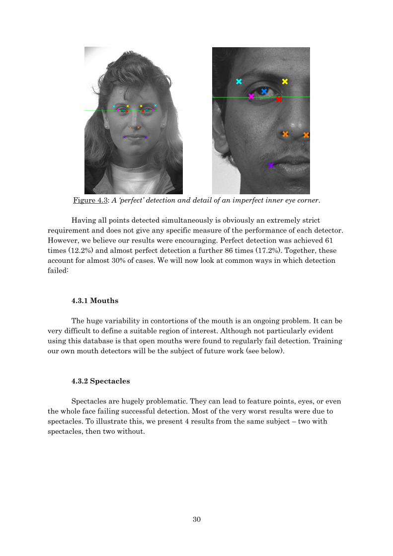
Figure 4.3: A ‘perfect’ detection and detail of an imperfect inner eye corner.

Having all points detected simultaneously is obviously an extremely strict

requirement and does not give any specific measure of the performance of each detector.

However, we believe our results were encouraging. Perfect detection was achieved 61

times (12.2%) and almost perfect detection a further 86 times (17.2%). Together, these

account for almost 30% of cases. We will now look at common ways in which detection

failed:

4.3.1 Mouths

The huge variability in contortions of the mouth is an ongoing problem. It can be

very difficult to define a suitable region of interest. Although not particularly evident

using this database is that open mouths were found to regularly fail detection. Training

our own mouth detectors will be the subject of future work (see below).

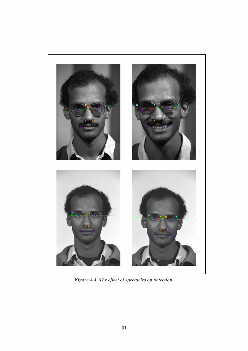
4.3.2 Spectacles

Spectacles are hugely problematic. They can lead to feature points, eyes, or even

the whole face failing successful detection. Most of the very worst results were due to

spectacles. To illustrate this, we present 4 results from the same subject – two with

spectacles, then two without.

31

Figure 4.4: The effect of spectacles on detection.

32

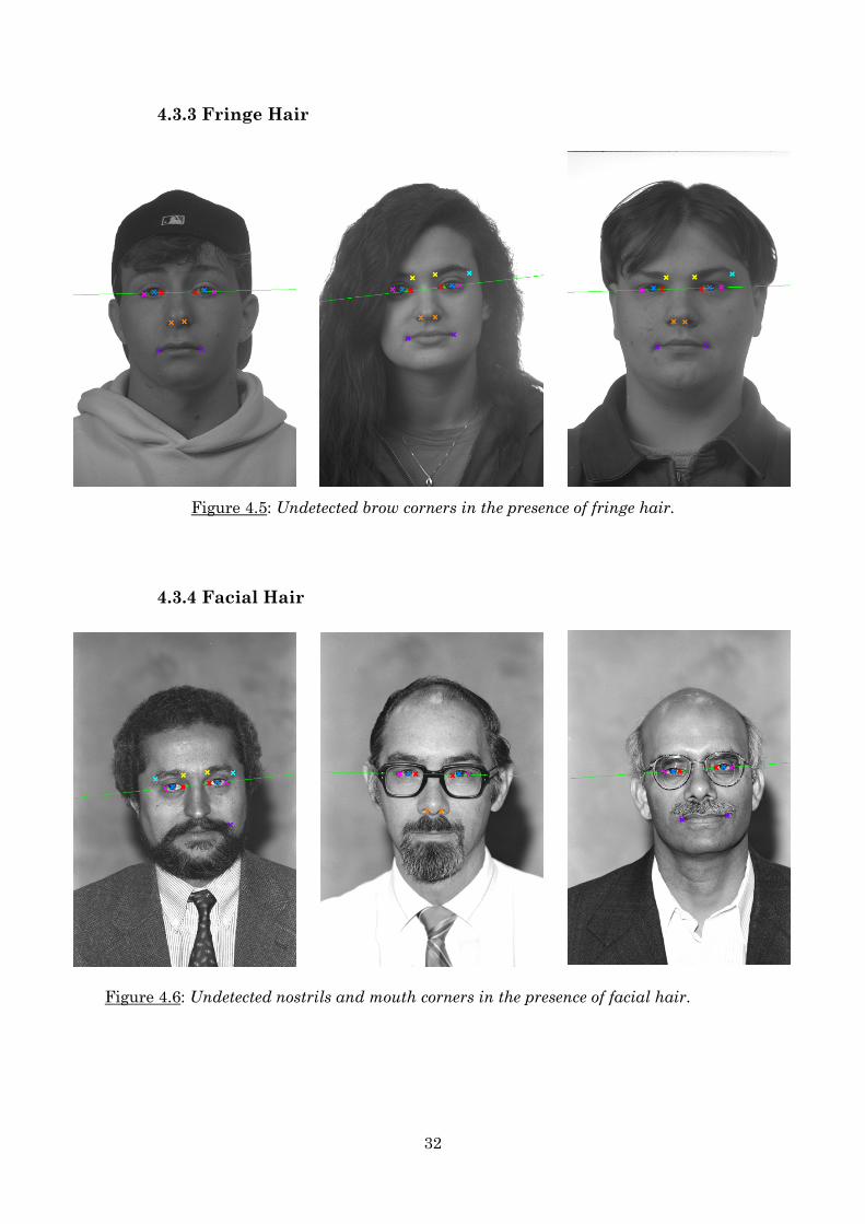
4.3.3 Fringe Hair

Figure 4.5: Undetected brow corners in the presence of fringe hair.

4.3.4 Facial Hair

Figure 4.6: Undetected nostrils and mouth corners in the presence of facial hair.

33

Chapter 5

Future Work and Conclusions

5.1 Future Work

Our system shows good potential and there is great scope for future development.

Perhaps the most important would be the incorporation of an explicit geometrical model

of the face. In particular, a better understanding of 3D shape would allow our system to

deal better with any rotations perpendicular to the image plane. This could perhaps be

achieved through a graph matching approach.

Such an approach could help to estimate the location of feature points that are

not detected. But, a geometrical model is also particularly relevant for our system

because each detector is capable of outputting several candidate coordinates. If some

geometric constraints were applied, then it may be possible to select the best overall

match from the set of candidate points.

Another approach to this problem would be to manipulate or alter the OpenCV

algorithm. Rather than getting multiple outputs that all meet certain criteria, it would

be desirable to obtain just one ‘best match’ in each case. At present, the ‘number of

neighbours’ parameter is used to find better matches, but choosing a specific value prior

to detection is limiting – it can lead to the output of zero or several detections in each

case. A better result would be to output only the coordinate with most neighbours in

each case.

Another important area for future work would be the development of our own

feature cascades. The face cascade was deemed to perform well, but feature detectors

were somewhat unreliable and did not seem to perform symmetrically. In particular, the

mouth detector presents a difficult problem. Analysis of the BioID Database showed that

the middle 90% of the width:height ratios of the mouth lay somewhere between 1.4 and

3.5. This is a huge variation, even with that set of natural expressions.

In testing, mouths often failed detection due to facial hair or being open. We

suggest that four mouth detectors should be trained to cope with all combinations of

beard/no beard and opened/closed. A specific challenge this would present would be

obtaining suitable training data. Even then, the great variation in facial hair could

cause problems and a new approach may be required.

To address the problems posed by spectacles, it may be beneficial to train a

glasses detector. However, since spectacles vary greatly in design and tend to sit

differently on different faces, even if we know the person is wearing glasses, this

problem may be especially difficult to address. The lenses tend to be non-lambertian

(appearance changes depending on angle of view) and the frames are generally opaque,

causing occlusion. It may be possible to attempt to fit any available information to a

deformable template, thus estimating the occluded parts within the constraints of this

template.

34

We briefly mentioned the possibility of horizontally mirroring detection cascades,

rather than having to flip image patches. Upon inspection of the cascade xml files, it

indeed seems that this would not be too difficult1. Here is an example of how a feature is

represented:

<feature>

<rects>

<_>10 0 2 9 -1.</_>

<_>7 3 2 3 3.</_></rects>

<tilted>1</tilted></feature>

.

.

.

The rectangles are given in standard OpenCV (x, y, width, height) form. The fifth

value is a weighting. So it seems it would just be a case of horizontally flipping these

rectangles within whatever detection window we have defined. For example, with our

13x13 window, (10, 0, 2, 9) would become (1,0,2,9).

5.2 Conclusions

Our work has identified weaknesses in previous colour-based approaches to

feature point detection. Through a careful exploration of human visual perception, we

put forward several arguments for an alternative approach, based on learning. We saw

how the greater level of abstraction offered by a high-dimensional feature space,

combined with correct feature types, could go some way towards mimicking basic neural

response and higher-level knowledge.

We then saw how the Viola-Jones method offers a sound basis for building such a

detection system. Novel feature sets were seen to offer somewhat more biological

responses, but we also noted that some sacrifice may be necessary in order to maintain

high frame rate. We thus identified the extended feature set, proposed by Lienhart et

al., to be a good compromise.

Our method of training detectors was necessarily meticulous. We sought to

normalise tilt and scale in order to optimise the training data. The precise nature of

both positive and negative samples was considered in detail. A total of 7 feature point

detectors were trained – allowing the detection of 14 points through image patch

mirroring. Our code was designed efficiently, to allow new detectors to be incorporated

quickly and easily.

Over all, detection results were very encouraging. Testing on an ‘easy’ sequence

of a single talking face, detection rates were largely above 90%. Testing on a much more

difficult dataset has also shown promising results and helped us to identify important

areas for future work.

1Thanks to Amanjit Dulai for helping me to understand the cascade xml files.

35

Bibliography

[1] S.F. Wang, S.H. Lai. Efficient 3D Face Reconstruction from a Single 2D Image by

Combining Statistical and Geometrical Information.

[2] D. Vukadinovic, M. Pantic. Fully Automatic Facial Feature Point Detection Using

Gabor Feature Based Boosted Classifiers.

[3] Z. Zhang et al. Comparison Between Geometry-Based and Gabor-Wavelets-Based

Facial Expression Recognition Using Multi-Layer Perceptron.

[4] T. Kanade et al. Automated Facial Expression Recognition Based on FACS Action

Units.

[5] P. Ekman, E. Rosenberg. What the face reveals: Basic and Applied Studies of

Spontaneous Expression Using the Facial Action Coding System, pages 372-383. Oxford

University Press, 1997.

[6] E. B. Goldstein. Sensation and Perception 7th Edition. Wadsworth, 2007.

[7] M. Malciu and F. Prêteux. Tracking facial features in video sequences using a

deformable model-based approach.

[8] R. Hassanpour et al. Adaptive Gaussian Mixture Model for Skin Color Segmentation.

[9] S. L. Phung et al. Skin Segmentation Using Color and Edge Information.

[10] K. Sandeep and A. Rajagopalan. Human Face Detection in Cluttered Color Images

Using Skin Color and Edge Information.

[11] J. Yang et al. Skin-Color Modeling and Adaptation.

[12] C. Stergiou and D. Siganos. Neural Networks.

Web Link: doc.ic.ac.uk/~nd/surprise_96/journal/vol4/cs11/report.html

[13] M. Reinders et al. Locating Facial Features in Image Sequences using Neural

Networks.

[14] L. Wiskott et al. Face Recognition by Elastic Bunch Graph Matching.

36

[15] Ville Hautamäki et al. Text-independent speaker recognition using graph matching.

[16] J. Y. Chen and B. Tiddeman. Multi-cue Facial Feature Detection and Tracking.

[17] D. Carrefio and X. Ginesta. Facial Image Recognition Using Neural Networks and

Genetic Algorithms.

[18] S.Uchida and H. Sakoe. A Survey of Elastic Matching Techniques for Handwritten

Character Recognition.

[19] M. Turk and A. Pentland. Eigenfaces for Recognition.

[20] L. I. Smith. A Tutorial on Principal Components Analysis.

[21] D. Cristinacce and T. Cootes. Facial Feature Detection using Adaboost with Shape

Constraints.

[22] M. H. Yang. Kernel Eigenfaces vs. Kernel Fisherfaces: Face Recognition Using

Kernel Methods.

[23] Y. Yong. Facial Expression Recognition and Tracking based on Distributed Locally

Linear Embedding and Expression Motion Energy.

[24] Y. P. Guan. Automatic extraction of lips based on multi-scale wavelet edge

detection.

[25] P. Viola and V. Jones. Robust Real-time Object Detection.

[26] P. Viola et al. Detecting Pedestrians Using Patterns of Motion and Appearance.

[27] R. Lienhart et al. Empirical Analysis of Detection Cascades of Boosted Classifiers

for Rapid Object Detection.

[28] J. Partzsch et al. Building Gabor Filters from Retinal Responses.

[29] J. Jones and L.Palmer. An evaluation of the Two-Dimensional Gabor Filter Model of

Simple Receptive Fields in Cat Striate Cortex.

37

[30] Lappeenranta University of Technology. GABOR – Gabor Features in Signal and

Image Processing.

Web link: it.lut.fi/project/gabor/

[31] M. Zhou and H. Wei. Face Verification Using Gabor Wavelets and AdaBoost.

[32] M. Castrillón-Santana. Face and Facial Feature Detection Evaluation.

Web link: alereimondo.no-ip.org/OpenCV/34

[33] BioID Technology Research. The BioID Face Database.

Web Link: bioid.com/downloads/facedb

[34] FGNET. Annotation of BioID Dataset.

Web Link: www-prima.inrialpes.fr/FGnet/data/11-BioID/bioid_points.html

[35] E. F. Glynn . RotateScanline Lab Report.

Web link: efg2.com/Lab/ImageProcessing/RotateScanline.htm

[36] FGNet. Talking Face Video.

Web link: www-prima.inrialpes.fr/FGnet/data/01-TalkingFace/talking_face.html

[37] National Institute of Standards Technology. The Color FERET Database.

Web link: face.nist.gov/colorferet/

[38] WillowGarage OpenCV wiki.

Web link: opencv.willowgarage.com

38

Appendix A

Preparing Training Samples and Implementing a Detector

This document provides a full step-by-step guide to creating our detectors. This

method has been specifically tailored to train classifier cascades for the detection of

facial feature points. The following C++ projects are required: “Create Logfile of

Positives”, “Create Database of Negatives” and “RobotVision”. The BioID Face Database

and ground truths[1] must also be installed and file paths should be updated in the C++

codes.

1. Create Positive Training Sample Database Descriptions

This stage requires the C++ project “Create Logfile of Positives”. This code reads

in the BioID Database ground truths for each image, and then creates a description log

of the positive sample(s) related to one of the 20 available feature points. A feature point

can either generate one positive sample or samples at several different scales (see

Project Report). First we must select the feature and number of sample scales:

1.1 enum{ THIS_FEATURE = 7 }; //Right Brow Outer Corner enum{ NSCALES = 3 };

Note: We want to describe left/right from our perspective – i.e. the opposite to BioID.

1.2 Executing the code will create the ‘log.txt’ description file. It should contain 1521

descriptions like this:

BioID_0000.pgm 3 184 163 25 25 185 164 23 23 186 165 21 21

BioID_0001.pgm 3 177 160 23 23 178 161 21 21 179 162 19 19

.

.

.

This format shows the image file name, number of positive samples in that

image, and then the (x, y, width, height) description(s) of the rectangular sample(s).

To use with OpenCV, these descriptions have to be converted to a ‘.vec’ file. This

is done at the command line, using the OpenCV executable ‘createsamples.exe’:

1.3 createsamples.exe –info log.txt –vec positives.vec –num 4563 –w 13 –h 13

This command takes the descriptions in ‘log.txt’ and creates ‘positives.vec’. In

this example, 3 scales were used for each of the 1521 images (giving 4563 total samples).

All of these samples are then rescaled to the same dimensions (here, we have 13x13).

Note: createsamples.exe can only rescale samples successfully if

iplWarpPerspectiveQ() is running correctly. This requires the line “#define HAVE_IPL” to

be added to _cvhaartraining.h[2].

39

2. Create Negative Training Sample Image Database

This stage requires the C++ project “Create Database of Negatives”. The code

generates 16 negative sample images per feature point, randomly located around that

feature point (see Project Report).

There are two changes to make in the code:

2.1 Choose a feature: enum{ THIS_FEATURE = 15 };

2.2 Set the path to save the negative image files: string neg_path = "H:\\Left Nostril Training\\bin\\Negatives\\";

Note: The number of images generated can be large (typically 22,000). Some

systems will hang if you try moving these files around, so it is advisable to set the

correct path within the code.

2222....3333 Executing the code creates a database of negative sample images (in the path

specified) and a log file of image names (in the project folder).

The log file should be copied to the image directory for the training stage.

3. Train Cascade of Classifiers

We now have our positive samples (in a ‘.vec’ file) and our negative samples (a

database of images with a text description file). These are now input to the OpenCV

Haar-like classifier training function, haartraining.exe. This process is computationally

intensive and can take days to complete (depending on system performance).

There are a number of input parameters which need to be considered. A typical

example is given:

3.1 haartraining.exe –data data/cascade –vec data/positives.vec –bg

negatives/neg.txt –npos 4563 –nneg 24336 –nstages 20 –mem 2000 –mode ALL

–w 20 –h 20 –minhitrate 0.995 –maxfalsealarm 0.5 –nonsym

The most important command-line parameters are:

-data Path to save cascade ---------------------------------------------------------- -- -vec Path to load positive samples ‘.vec’ -bg Path to description of negative samples ‘.txt’ -npos Number of positive samples -nneg Number of negative samples -nstages Number of cascade stages -nsplits Number of tree splits (See [3], pg6) -nonsym Must be set if feature is not left-right symmetrical -mem Physical memory to be used (megabytes) -minhitrate Minimum hit rate -maxfalsealarm Maximum false alarm rate -mode ‘BASIC’ uses only upright features, ‘ALL’ uses full set. -w and -h Width and height of training samples

40

+----+----+-+---------+---------+---------+---------+

| N |%SMP|F| ST.THR | HR | FA | EXP. ERR|

+----+----+-+---------+---------+---------+---------+

| 18| 79%|-|-1.486423| 0.995035| 0.899966| 0.128105|

+----+----+-+---------+---------+---------+---------+

| 19| 79%|-|-1.434926| 0.995035| 0.872503| 0.155258|

+----+----+-+---------+---------+---------+---------+

| 20| 79%|-|-1.450002| 0.995035| 0.875973| 0.147311|

+----+----+-+---------+---------+---------+---------+

| 21|100%|-|-1.450002| 0.995035| 0.875973| 0.147311|

+----+----+-+---------+---------+---------+---------+

| 22|100%|-|-1.450002| 0.995035| 0.875973| 0.147311|

+----+----+-+---------+---------+---------+---------+

Note: Often the training process will not complete. After a number of stages, it

may become impossible for the minhitrate and maxfalsealarm criteria to be

simultaneously achieved.

For example, the command-line output below shows a cascade that has failed to

meet training requirements during Stage 6. We can see that increasing the number of

features (N) beyond 20 has no further effect on hit rate (HR) and false alarm rate (FA):

When this happens, it is necessary to terminate the program (Ctrl+C) and

slacken the training parameters. In general, a small decrease/increase in

maxhitrate/minfalsealarm will allow that stage to complete successfully.

It is difficult to say how many stages is ‘enough’. This will depend heavily on the

required application. In general, extra stages will decrease overall false alarms, but will

also decrease hit rate. The best way to evaluate performance is to test the cascade at

various stages.

4. Convert Cascade

In order to use the cascade for detection, the data first has to be converted to xml

format. This is done using convert_cascade.exe:

4.1 convert_cascade.exe --size="13x13" data/cascade data/LeftNostril5.xml

This classifier cascade is now ready to use for detection. OpenCV does have a

performance testing tool (performance.exe), but this is not relevant for feature point

detection due to the constraints we require to be imposed on local background

information. Instead, we must implement the detector directly in our C++ code.

5. Test Cascade

This stage requires the main C++ feature point detection project “RobotVision”.

The code uses various classifier cascades to detect feature points within various regions

of interest (ROI). Before detection can begin, there are numerous parameters that must

first be initialised for every detector. The code has been very carefully designed to make

this simple.

41

Each

det

ecto

r is

arr

an

ged

in

to a

str

uct

ure

wh

ose

mem

ber

s n

eed

to

be

init

iali

sed

. W

e w

ill

use

th

e ou

ter

righ

t bro

w a

s an

exam

ple

poi

nt:

5 555. ...1 111

T

he

foll

owin

g p

ara

met

ers

shou

ld b

e in

itia

lise

d.

Th

e valu

es t

hey

req

uir

e are

obvio

us

from

loo

kin

g a

t th

e co

de:

Pa

ra

me

ter

Ty

pe

D

es

cr

ipti

on

In

itia

lise

in

m_RightBrowOuter.ROI

CvRect

Re

cta

ng

ula

r re

gio

n o

f in

tere

st f

or

de

tect

ion

m

ain

m_RightBrowOuter.cascade

CvHaarClassifierCascade*

Ca

sca

de

re

ad

in

fro

m o

ur

xml

file

co

nst

ruct

or

m_RightBrowOuter.IsPoint

bool

Tru

e f

or

fea

ture

po

ints

, fa

lse

fo

r fe

atu

res

con

stru

cto

r m_RightBrowOuter.OnRightSide bool

Tru

e i

f fe

atu

re (

po

int)

is

on

th

e r

igh

t o

f th

e f

ace

co

nst

ruct

or

m_RightBrowOuter.OK

bool

Tru

e i

f fe

atu

re (

po

int)

ha

s b

ee

n s

ucc

ess

full

y d

ete

cte

d

con

stru

cto

r m_RightBrowOuter.HaarParams

double[4]

Vio

la-J

on

es

de

tect

ion

pa

ram

ete

rs*

(se

e b

elo

w)

con

stru

cto

r

*Vio

la-J

on

es

de

tect

ion

pa

ram

ete

rs:

Pa

ram

ete

r D

efi

nit

ion

D

esc

rip

tio

n

HaarParams[0]

S

cale

Fa

cto

r H

aa

r-li

ke

fe

atu

res

incr

ea

se b

y a

sca

le o

f <HaarParams[0]>

on

ea

ch i

tera

tio

n

HaarParams[1]

M

in.

Ne

igh

bo

urs

P

osi

tive

ma

tch

re

qu

ire

s a

clu

ste

r w

ith

at

lea

st <HaarParams[1]>

ne

igh

bo

urs

HaarParams[2], HaarParams[3]

M

in.

Siz

e

Init

ial

Ha

ar-

lik

e f

ea

ture

siz

e i

s <HaarParams[2]

> x

<HaarParams[3]

>

Wit

h e

ver

yth

ing c

orre

ctly

in

itia

lise

d, th

e d

etec

tion

fu

nct

ion

can

now

be

call

ed f

rom

th

e m

ain

fu

nct

ion

:

5.2 DetectFeaturePoint(&m_RightBrowOuter, temp_img);

Fin

all

y,

the

det

ecte

d f

eatu

re p

oin

t ca

n b

e d

isp

layed

by a

lter

ing t

he DrawFeaturePoints f

un

ctio

n:

5.3

if(m_RightBrowOuter.OK)

DrawCross(m_img, 4, m_RightBrowOuter.point, CV_RGB( 255,255,0)

42

References (for Appendix A):

[1] The BioID Face Database with FGnet Markup Scheme. Web link: bioid.com/downloads/facedb

[2] F. Adolf. “OpenCV's Rapid Object Detection”.

Web link: robotik.inflomatik.info/other/opencv/OpenCV_ObjectDetection_HowTo.pdf

[3] R. Lienhart, A. Kuranov and Vadim Pisarevsky. “Empirical Analysis of Detection

Cascades of Boosted Classifiers for Rapid Object Detection”.

[4] OpenCV Documentation. “Rapid Object Detection with a Cascade of Boosted

Classifiers Based on Haar-like Features”.

[5] Asian Institute of Technology, Computer Vision Wiki. “Haar Training for Pedestrian

Detection”.

Web link: webeng.cs.ait.ac.th/cvwiki/opencv:tutorial:haartraining