98

/Author (David Joyner and William Stein) /Title (SAGE Tutorial)
SAGE Tutorial
Release 2006.07.30
David Joyner and William Stein
July 30, 2006
Email: [email protected], [email protected]

Copyright© 2006 William A. Stein. All rights reserved.
See the end of this document for complete license and permissions information.

Abstract
SAGE is Software for Algebra and Geometry Experimentation. It is free and open sourcesoftware for number theory, algebra, and geometry computations. This tutorial contains anoverview of SAGE.


CONTENTS
1 Introduction 11.1 Installation . . . . . . . . . . . . . . . . . . . . . . . . . . . . . . . . . . . . 11.2 Ways to Use SAGE . . . . . . . . . . . . . . . . . . . . . . . . . . . . . . . 21.3 Longterm Goals for SAGE . . . . . . . . . . . . . . . . . . . . . . . . . . . 2
2 A Guided Tour 52.1 Basic, and not-so-basic, Rings . . . . . . . . . . . . . . . . . . . . . . . . . . 52.2 Polynomials . . . . . . . . . . . . . . . . . . . . . . . . . . . . . . . . . . . . 82.3 Number Theory . . . . . . . . . . . . . . . . . . . . . . . . . . . . . . . . . 142.4 Linear Algebra . . . . . . . . . . . . . . . . . . . . . . . . . . . . . . . . . . 192.5 Finite Groups . . . . . . . . . . . . . . . . . . . . . . . . . . . . . . . . . . . 232.6 Elliptic Curves . . . . . . . . . . . . . . . . . . . . . . . . . . . . . . . . . . 252.7 Plotting . . . . . . . . . . . . . . . . . . . . . . . . . . . . . . . . . . . . . . 282.8 Calculus . . . . . . . . . . . . . . . . . . . . . . . . . . . . . . . . . . . . . . 302.9 Algebraic Geometry . . . . . . . . . . . . . . . . . . . . . . . . . . . . . . . 372.10 Modular Forms . . . . . . . . . . . . . . . . . . . . . . . . . . . . . . . . . . 38
3 The Interactive Shell 413.1 Your SAGE session . . . . . . . . . . . . . . . . . . . . . . . . . . . . . . . . 413.2 Logging Input and Output . . . . . . . . . . . . . . . . . . . . . . . . . . . 433.3 Paste Ignores Prompts . . . . . . . . . . . . . . . . . . . . . . . . . . . . . . 453.4 Timing Commands . . . . . . . . . . . . . . . . . . . . . . . . . . . . . . . . 453.5 Errors and Exceptions . . . . . . . . . . . . . . . . . . . . . . . . . . . . . . 473.6 Reverse Search and Tab Completion . . . . . . . . . . . . . . . . . . . . . . 493.7 Integrated Help System . . . . . . . . . . . . . . . . . . . . . . . . . . . . . 503.8 Saving and Loading Individual Objects . . . . . . . . . . . . . . . . . . . . . 523.9 Saving and Loading Complete Sessions . . . . . . . . . . . . . . . . . . . . . 553.10 The Notebook Interface . . . . . . . . . . . . . . . . . . . . . . . . . . . . . 56
4 Interfaces 594.1 GP/PARI . . . . . . . . . . . . . . . . . . . . . . . . . . . . . . . . . . . . . 594.2 GAP . . . . . . . . . . . . . . . . . . . . . . . . . . . . . . . . . . . . . . . 61
i

4.3 Singular . . . . . . . . . . . . . . . . . . . . . . . . . . . . . . . . . . . . . . 624.4 Maxima . . . . . . . . . . . . . . . . . . . . . . . . . . . . . . . . . . . . . . 63
5 Programming 675.1 Loading and Attaching SAGE �les . . . . . . . . . . . . . . . . . . . . . . . 675.2 Creating Compiled Code . . . . . . . . . . . . . . . . . . . . . . . . . . . . . 685.3 Standalone Python/SAGE Scripts . . . . . . . . . . . . . . . . . . . . . . . . 695.4 Data Types . . . . . . . . . . . . . . . . . . . . . . . . . . . . . . . . . . . . 695.5 Lists, Tuples, and Sequence . . . . . . . . . . . . . . . . . . . . . . . . . . . 715.6 Dictionaries . . . . . . . . . . . . . . . . . . . . . . . . . . . . . . . . . . . . 745.7 Sets . . . . . . . . . . . . . . . . . . . . . . . . . . . . . . . . . . . . . . . . 755.8 Iterators . . . . . . . . . . . . . . . . . . . . . . . . . . . . . . . . . . . . . . 765.9 Loops, Functions, Control Statements, and Comparisons . . . . . . . . . . . 775.10 Adding Your Own Methods to a SAGE Class . . . . . . . . . . . . . . . . . 805.11 Pro�ling . . . . . . . . . . . . . . . . . . . . . . . . . . . . . . . . . . . . . . 82
6 Afterword 856.1 Why Python? . . . . . . . . . . . . . . . . . . . . . . . . . . . . . . . . . . . 856.2 I would like to contribute somehow. How can I? . . . . . . . . . . . . . . . . 876.3 How do I reference SAGE? . . . . . . . . . . . . . . . . . . . . . . . . . . . . 88
Index 91
ii
CHAPTER
ONE
Introduction
This tutorial will likely take you about 2�3 hours to work through.
Though much of SAGE is implemented using Python, no Python background is needed toread this tutorial. (Some background on Python will be needed by the heavy SAGE user,but this is not the place for that.) If you just want to quickly try out SAGE, this is the placeto start. For example:
sage: 2 + 2
4
sage: factor(2006)
2 * 17 * 59
sage: A = MatrixSpace(QQ, 4)(range(16)); A
[ 0 1 2 3]
[ 4 5 6 7]
[ 8 9 10 11]
[12 13 14 15]
sage: factor(A.charpoly())
x^2 * (x^2 - 30*x - 80)
sage: E = EllipticCurve([1,2,3,4,5]);
sage: E
Elliptic Curve defined by y^2 + x*y + 3*y = x^3 + 2*x^2 + 4*x + 5
over Rational Field
sage: E.anlist(10)
[0, 1, 1, 0, -1, -3, 0, -1, -3, -3, -3]
1.1 Installation
If you do not have SAGE installed on a computer, and just want to try some SAGE command,you might try the SAGE online calculator at http://modular.math.washington.edu/calc.
1
See the document Installing SAGE in the documentation section of the main webpage ofSAGE [SA] for instructions on installing SAGE on your computer. Here we merely make twocomments.
1. The SAGE download �le comes with �batteries included�. In other words, althoughSAGE uses Python, IPython, PARI, GAP, Singular, Maxima, NTL, GMP, and soon, you do not need to install them separately as they are included with the SAGEdistribution. However, to use certain SAGE features, e.g., Macaulay or KASH, youmust install the relevant optional SAGE package. Macaulay and KASH are SAGEpackages (type sage -optional for a list of available optional packages). For theexact versions of the standard SAGE packages, go to the SAGE website and choose�Download� then �standard�.
2. The pre-compiled binary version of SAGE (found on the SAGE web site) may be easierand quicker to install than the source code version. Just unpack the �le and run sage.
1.2 Ways to Use SAGE
You can use SAGE
� via an interactive shell (Chapter 3),
� via the notebook interface (see the section on the Notebook in the reference manualand �3.10 below),
� by writing interpreted and compiled programs in SAGE (see Section 5.1 and 5.2), and
� by wring a write stand-alone Python scripts that use the SAGE library (see Section 5.3).
1.3 Longterm Goals for SAGE
� Useful: SAGE's intended audience includes not only researchers in mathematics butalso teachers of mathematics. The aim is to provide a software that can be used toexplore and experiment with mathematical constructions in algebra, geometry, numbertheory, calculus, etc. SAGE will help make it easier to interactively experiment withmathematical objects.
� E�cient: Be fast. SAGE uses highly-optimized mature software like GMP, PARI,GAP, and NTL, which is often very fast at certain operations.
� Free and open source: The source code must be freely available and readable, sousers can understand what the system is really doing and more easily extend it. Justas mathematicians gain a deeper understanding of a theorem by carefully reading or at
2 Chapter 1. Introduction

least skimming the proof, people who do computations should be able to understandhow the calculations work by reading documented source code. If you use SAGE todo computations in a paper you publish, you can rest assured that your readers willalways have free access to SAGE and all its source code, and you are even allowed toarchive and re-distribute the version of SAGE you used.
� Easy to compile: SAGE should be easy to compile from source for Linux, OS X andWindows users. This provides more �exibility for users to modify the system.
� Cooperation: Provide robust interfaces to most other computer algebra systems,including PARI, GAP, Singular, Maxima, KASH, Magma, Maple, and Mathematica.SAGE is meant to unify existing math software, rather than compete with it. SAGE isnot about reinventing the wheel.
� Well documented: Tutorial, programming guide, reference manual, and how-to, withnumerous examples and discussion of background mathematics.
� Extensible: Be able to de�ne new data types or derive from built-in types, and usecode written in a range of languages.
� User friendly: Easy to understand what functionality is provided for a given objectand view documentation and source code. Also attain a high level of user support(maybe similar to what GAP currently o�ers its users).
1.3. Longterm Goals for SAGE 3

4

CHAPTER
TWO
A Guided Tour
This section is a guided tour of some of what is available in SAGE 1.0. For more examples,see the SAGE documentation �SAGE constructions�, which is intended to answer the generalquestion �How do I construct ...?�.
2.1 Basic, and not-so-basic, Rings
We illustrate some basic rings in SAGE. For example, the �eld Q of rational numbers maybe referred to using either RationalField() or QQ:
sage: RationalField()
Rational Field
sage: QQ
Rational Field
sage: 1/2 in QQ
True
The decimal number 1.2 is considered in Q, since there is a coercion map from the reals tothe rationals:
sage: 1.2 in QQ
True
However, the following doesn't, since there is no coercion:
sage: I = ComplexField().0
sage: I in QQ
False
Also, of course, the symbolic constant π is not in Q:
5

sage: pi in QQ
False
If you use QQ as a variable, you can still fetch the rational numbers using the commandRationalField(). By the way, some other pre-de�ned SAGE rings include the integers ZZ,the real numbers RR, the complex numbers CC (which uses I (or i), as usual, for the squareroot of −1). We discuss polynomial rings in Section 2.2.
Do not rede�ne Integer or RealNumber unless you really know what you are doing. Theyare used by the SAGE interpreter to wrap integer and real literals. For example, if you typeInteger = int, then integer literals will behave as they usually do in Python, so e.g., 4/3evaluates to the Python int 1. For example
sage: 4/3
4/3
sage: parent(_)
Rational Field
sage: prev = Integer
sage: Integer = int
sage: 4/3
1
sage: parent(_)
<type 'int'>
sage: Integer = prev
sage: 4/3
4/3
Now we illustrate some arithmetic involving various numbers.
6 Chapter 2. A Guided Tour

sage: a, b = 4/3, 2/3
sage: a + b
2
sage: 2*b == a
True
sage: parent(2/3)
Rational Field
sage: parent(4/2)
Rational Field
sage: 2/3 + 0.1 # automatic coercion before addition
0.76666666666666661
sage: 0.1 + 2/3 # coercion rules are symmetric in SAGE
0.76666666666666661
sage: z = a + b*I
sage: z
1.3333333333333333 + 0.66666666666666663*I
sage: z.real() == a # automatic coercion before comparision
True
sage: QQ(11.1)
111/10
Python is dynamically typed, so the value referred to by each variable has a type associatedwith it, but a given variable may hold values of any Python type within a given scope:
sage: a = 5
sage: type(a)
<type 'integer.Integer'>
sage: a = 5/3
sage: type(a)
<type 'rational.Rational'>
sage: a = 'hello'
sage: type(a)
<type 'str'>
The C programming language, which is statically typed, is much di�erent; a variable declaredto hold an int can only hold an int in its scope.
The �eld of p-adic numbers is implements as well:
2.1. Basic, and not-so-basic, Rings 7

sage: K = Qp(11); K.prec(10)
sage: a = K(211/17); a
4 + 4*11 + 11^2 + 7*11^3 + 9*11^5 + 5*11^6 + 4*11^7 + 8*11^8 + 7*11^9 +
O(11^10)
sage: a.denominator()
1
sage: b = K(3211/11^2); b
10*11^-2 + 5*11^-1 + 4 + 2*11 + O(11^Infinity)
sage: b.denominator()
121
Rings of integers in p-adic �elds or number �elds other than Q have not yet been imple-mented. However,a number of related methods are already implemented in the NumberFieldclass.
sage: x = PolynomialRing(QQ).gen()
sage: K = NumberField(x^3 + x^2 - 2*x + 8, 'a')
sage: K.integral_basis()
[1, a, 1/2*a^2 + 1/2*a]
sage: K.galois_group() # requires optional GAP database package
Transitive group number 2 of degree 3
sage: K.polynomial_quotient_ring()
Univariate Quotient Polynomial Ring in a over Rational Field with modulus x^3 + x^2 - 2*x + 8
sage: K.units()
[3*a^2 + 13*a + 13]
sage: K.discriminant()
-503
sage: K.class_group()
Abelian group on 0 generators () with invariants []
sage: K.class_number()
1
2.2 Polynomials
In this section we illustrate how to create and use polynomials in SAGE.
2.2.1 Univariate Polynomials
There are three ways to create polynomial rings.
8 Chapter 2. A Guided Tour
sage: R = PolynomialRing(QQ, 'x')
sage: R
Univariate Polynomial Ring in x over Rational Field
An alternate way is
sage: S = QQ['x']
sage: S == R
True
A third very convenient way is
sage: R.<x> = PolynomialRing(QQ)
or
sage: R.<x> = QQ['x']
This has the additional side e�ect that it de�nes the variable x to be the indeterminate ofthe polynomial ring. (Note that the third way is very similar to the constructor notation inMAGMA, and just as in MAGMA it can be used for a wide range of objects.)
The indeterminate of the polynomial ring is the 0th generator:
sage: R = PolynomialRing(QQ, 'x')
sage: x = R.0
sage: x in R
True
Alternatively, you can obtain both the ring and its generator, or just the generator duringring creation as follows:
sage: R, x = QQ['x'].objgen()
sage: x = QQ['x'].gen()
sage: R, x = objgen(QQ['x'])
sage: x = gen(QQ['x'])
Finally we do some arithmetic in Q[x].
2.2. Polynomials 9

sage: R, x = QQ['x'].objgen()
sage: f = 2*x^7 + 3*x^2 - 15/19
sage: f^2
4*x^14 + 12*x^9 - 60/19*x^7 + 9*x^4 - 90/19*x^2 + 225/361
sage: cyclo = R.cyclotomic_polynomial(7); cyclo
x^6 + x^5 + x^4 + x^3 + x^2 + x + 1
sage: g = 7 * cyclo * x^5 * (x^5 + 10*x + 2)
sage: g
7*x^16 + 7*x^15 + 7*x^14 + 7*x^13 + 77*x^12 + 91*x^11 + 91*x^10 + 84*x^9
+ 84*x^8 + 84*x^7 + 84*x^6 + 14*x^5
sage: F = factor(g); F
(7) * x^5 * (x^5 + 10*x + 2) * (x^6 + x^5 + x^4 + x^3 + x^2 + x + 1)
sage: F.unit()
7
sage: list(F)
[(x, 5), (x^5 + 10*x + 2, 1), (x^6 + x^5 + x^4 + x^3 + x^2 + x + 1, 1)]
Notice that that the factorization correctly takes into account and records the unit part,unlike many other programs (e.g., PARI, Magma).
If you were to use, e.g., the R.cyclotomic_polynomial function a lot for some researchproject, in addition to citing SAGE you should make an attempt to �nd out what componentof SAGE is being used to actually compute the cyclotomic polynomial and cite that as well.In this case, if you type R.cyclotomic_polynomial?? to see the source code, you'll quicklysee a line f = pari.polcyclo(n) which means that PARI is being used for computation ofthe cyclotomic polynomial. Cite PARI in your work as well.
Dividing two polynomials constructs an element of the fraction �eld.
sage: x = QQ['x'].0
sage: f = x^3 + 1; g = x^2 - 17
sage: h = f/g; h
(x^3 + 1)/(x^2 - 17)
sage: h.parent()
Fraction Field of Univariate Polynomial Ring in x over Rational Field
Using Laurent series, one can compute series expansions in the fraction �eld of QQ[x]:
sage: R = LaurentSeriesRing(QQ, 'x'); R
Laurent Series Ring in x over Rational Field
sage: x = R.gen()
sage: 1/(1-x) + O(x^10)
1 + x + x^2 + x^3 + x^4 + x^5 + x^6 + x^7 + x^8 + x^9 + O(x^10)
10 Chapter 2. A Guided Tour

If we name the variable di�erently, we obtain a di�erent univariate polynomial ring.
sage: R.<x> = PolynomialRing(QQ)
sage: S.<y> = PolynomialRing(QQ)
sage: x == y
False
sage: R == S
False
sage: R(y)
x
sage: R(y^2 - 17)
x^2 - 17
The ring is determined by the variable. Note that making another ring with variable calledx does return a di�erent ring.
sage: R = PolynomialRing(QQ, "x")
sage: T = PolynomialRing(QQ, "x")
sage: R == T
True
sage: R is T
False
sage: R.0 == T.0
True
SAGE also has support for power series and Laurent series rings over any base ring. In thefollowing example we create an element of F7[[T ]] and divide to create an element of F7((T )).
sage: R = PowerSeriesRing(GF(7), 'T'); R
Power Series Ring in T over Finite Field of size 7
sage: T = R.0
sage: f = T + 3*T^2 + T^3 + O(T^4)
sage: f^3
T^3 + 2*T^4 + 2*T^5 + O(T^6)
sage: 1/f
T^-1 + 4 + T + O(T^2)
sage: parent(1/f)
Laurent Series Ring in T over Finite Field of size 7
You can also create power series rings using a double-brackets shorthand:
2.2. Polynomials 11

sage: GF(7)[['T']]
Power Series Ring in T over Finite Field of size 7
2.2.2 Multivariate Polynomials
To work with polynomials of several variables, we declare the polynomial ring and variables�rst, in one of two ways.
sage: R = MPolynomialRing(GF(5),3,"z")
sage: R
Polynomial Ring in z0, z1, z2 over Finite Field of size 5
Just as for univariate polynomials, there is an alternative more compact notation:
sage: GF(5)['z0, z1, z2']
Polynomial Ring in z0, z1, z2 over Finite Field of size 5
Also, if you want the variable names to be single letters then you can use the followingshorthand:
sage: MPolynomialRing(GF(5), 3, 'xyz')
Polynomial Ring in x, y, z over Finite Field of size 5
Next lets do some arithmetic.
sage: z = GF(5)['z0, z1, z2'].gens()
sage: z
(z0, z1, z2)
sage: (z[0]+z[1]+z[2])^2
z2^2 + 2*z1*z2 + z1^2 + 2*z0*z2 + 2*z0*z1 + z0^2
You can also use more mathematical notation to construct a polynomial ring.
12 Chapter 2. A Guided Tour

sage: R = GF(5)['x,y,z']
sage: x,y,z = R.gens()
sage: QQ['x']
Univariate Polynomial Ring in x over Rational Field
sage: QQ['x,y'].gens()
(x, y)
sage: QQ['x'].objgens()
(Univariate Polynomial Ring in x over Rational Field, (x,))
Multivariate polynomials are implemented in SAGE using the Python dictionaries and the�distributive representation� of a polynomial. SAGE makes some use of Singular [Si], e.g.,for computation of gcd's and Gröbner basis of ideals.
sage: R, (x, y) = PolynomialRing(RationalField(), 2, 'xy').objgens()
sage: f = (x^3 + 2*y^2*x)^2
sage: g = x^2*y^2
sage: f.gcd(g)
x^2
Next we create the ideal (f, g) generated by f and g, by simply multiplying (f,g) by R (wecould also write ideal([f,g])) or ideal(f,g).
sage: I = (f, g)*R; I
Ideal (x^2*y^2, 4*x^2*y^4 + 4*x^4*y^2 + x^6) of Polynomial Ring in x, y over Rational Field
sage: B = I.groebner_basis(); B
[x^2*y^2, 4*x^2*y^4 + 4*x^4*y^2 + x^6]
sage: x^2 in I
False
Incidentally, the Groebner basis above is not just a list but an immutable sequence. Thismeans that it has a universe, parent, and cannot be changed (which is good because changingthe basis would break other routines that use the Groebner basis).
sage: B.parent()
Category of sequences in Polynomial Ring in x, y over Rational Field
sage: B.universe()
Polynomial Ring in x, y over Rational Field
sage: B[1] = x
Traceback (most recent call last):
...
ValueError: object is immutable; please change a copy instead.
2.2. Polynomials 13
Some (read: not as much as we would like) commutative algebra is available in SAGE,implemented via Singular. For example, we can compute the primary decomposition andassociated primes of I:
ssage: I.primary_decomposition()
[Ideal (x^2) of Polynomial Ring in x, y over Rational Field,
Ideal (y^2, 4*x^2*y^4 + 4*x^4*y^2 + x^6) of Polynomial Ring in x, y over Rational Field]
sage: I.associated_primes()
[Ideal (x) of Polynomial Ring in x, y over Rational Field,
Ideal (y, x) of Polynomial Ring in x, y over Rational Field]
2.3 Number Theory
SAGE has extensive functionality for number theory. For example, we can do arithmetic inZ/NZ as follows:
sage: R = IntegerModRing(97)
sage: a = R(2) / R(3)
sage: a
33
sage: a.rational_reconstruction()
2/3
sage: b = R(47)
sage: b^20052005
50
sage: b.modulus()
97
sage: b.is_square()
True
SAGE contains standard number theoretic functions. For example,
14 Chapter 2. A Guided Tour

sage: gcd(515,2005)
5
sage: factor(2005)
5 * 401
sage: c = factorial(25); c
15511210043330985984000000
sage: [valuation(c,p) for p in prime_range(2,23)]
[22, 10, 6, 3, 2, 1, 1, 1]
sage: next_prime(2005)
2011
sage: previous_prime(2005)
2003
sage: divisors(28); sum(divisors(28)); 2*28
[1, 2, 4, 7, 14, 28]
56
56
Perfect!
SAGE's sigma(n,k) function adds up the kth powers of the divisors of n (note the order ofn and k!):
sage: sigma(28,0); sigma(28,1); sigma(28,2)
6
56
1050
We next illustrate the extended Euclidean algorithm, the Euler's φ-function, and the Chineseremainder theorem:
2.3. Number Theory 15

sage: d,u,v = xgcd(12,15)
sage: d == u*12 + v*15
True
sage: inverse_mod(3,2005)
1337
sage: 3 * 1337
4011
sage: n = 2005
sage: prime_divisors(n)
[5, 401]
sage: phi = n*prod([1 - 1/p for p in prime_divisors(n)]); phi
1600
sage: euler_phi(2005)
1600
sage: prime_to_m_part(n, 5)
401
We next verify something about the 3n + 1 problem.
sage: n = 2005
sage: for i in range(1000):
n = 3*odd_part(n) + 1
if odd_part(n)==1:
print i
break
38
Finally we illustrate the Chinese remainder theorem.
16 Chapter 2. A Guided Tour

sage: x = crt(2, 1, 3, 5); x
-4
sage: x % 3 # x mod 3 = 2
2
sage: x % 5 # x mod 5 = 1
1
sage: [binomial(13,m) for m in range(14)]
[1, 13, 78, 286, 715, 1287, 1716, 1716, 1287, 715, 286, 78, 13, 1]
sage: [binomial(13,m)%2 for m in range(14)]
[1, 1, 0, 0, 1, 1, 0, 0, 1, 1, 0, 0, 1, 1]
sage: [kronecker(m,13) for m in range(1,13)]
[1, -1, 1, 1, -1, -1, -1, -1, 1, 1, -1, 1]
sage: n = 10000; sum([moebius(m) for m in range(1,n)])
-23
sage: list(partitions(4))
[(1, 1, 1, 1), (1, 1, 2), (2, 2), (1, 3), (4,)]
2.3.1 Dirichlet Characters
A Dirichlet character is the extension of a homomorphism
(Z/NZ)∗ → R∗,
for some ring R, to the map Z/NZ → R obtained by sending those x ∈ Z/NZ withgcd(N, x) > 1 to 0.
sage: G = DirichletGroup(21)
sage: list(G)
[[1, 1], [-1, 1], [1, zeta6], [-1, zeta6], [1, zeta6 - 1],
[-1, zeta6 - 1], [1, -1], [-1, -1], [1, -zeta6], [-1, -zeta6],
[1, -zeta6 + 1], [-1, -zeta6 + 1]]
sage: G.gens()
([-1, 1], [1, zeta6])
sage: len(G)
12
Having created the group, we next create an element and compute with it.
2.3. Number Theory 17

sage: chi = G.1; chi
[1, zeta6]
sage: chi.values()
[0, 1, zeta6 - 1, 0, -zeta6, -zeta6 + 1, 0, 0, 1, 0, zeta6,
-zeta6, 0, -1, 0, 0, zeta6 - 1, zeta6, 0, -zeta6 + 1, -1]
sage: chi.conductor()
7
sage: chi.modulus()
21
sage: chi.order()
6
It is also possible to compute the action of the Galois group Gal(Q(ζn)/Q) on these char-acters, as well as the direct product decomposition corresponding to the factorization of themodulus.
sage: G.galois_orbits()
[
[[1, 1]],
[[-1, 1]],
[[1, zeta6], [1, -zeta6 + 1]],
[[-1, zeta6], [-1, -zeta6 + 1]],
[[1, zeta6 - 1], [1, -zeta6]],
[[-1, zeta6 - 1], [-1, -zeta6]],
[[1, -1]],
[[-1, -1]]
]
sage: G.decomposition()
[
Group of Dirichlet characters of modulus 3 over Cyclotomic Field of order 6 and degree 2,
Group of Dirichlet characters of modulus 7 over Cyclotomic Field of order 6 and degree 2
]
Next, we construct the group of Dirichlet character mod 20, but with values in Q(i):
sage: G = DirichletGroup(20)
sage: G.list()
[[1, 1], [-1, 1], [1, zeta4], [-1, zeta4], [1, -1],
[-1, -1], [1, -zeta4], [-1, -zeta4]]
We next compute several invariants of G:
18 Chapter 2. A Guided Tour
sage: G.gens()
([-1, 1], [1, zeta4])
sage: G.unit_gens()
[11, 17]
sage: G.zeta()
zeta4
sage: G.zeta_order()
4
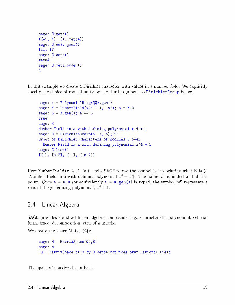
In this example we create a Dirichlet character with values in a number �eld. We explicitlyspecify the choice of root of unity by the third argument to DirichletGroup below.
sage: x = PolynomialRing(QQ).gen()
sage: K = NumberField(x^4 + 1, 'a'); a = K.0
sage: b = K.gen(); a == b
True
sage: K
Number Field in a with defining polynomial x^4 + 1
sage: G = DirichletGroup(5, K, a); G
Group of Dirichlet characters of modulus 5 over
Number Field in a with defining polynomial x^4 + 1
sage: G.list()
[[1], [a^2], [-1], [-a^2]]
Here NumberField(x^4 1, 'a')+ tells SAGE to use the symbol �a� in printing what K is (a�Number Field in a with de�ning polynomial x4 + 1�). The name �a� is undeclared at thispoint. Once a = K.0 (or equivalently a = K.gen()) is typed, the symbol �a� represents aroot of the generating polynomial, x4 + 1.
2.4 Linear Algebra
SAGE provides standard linear algebra commands, e.g., characteristic polynomial, echelonform, trace, decomposition, etc., of a matrix.
We create the space Mat3×3(Q):
sage: M = MatrixSpace(QQ,3)
sage: M
Full MatrixSpace of 3 by 3 dense matrices over Rational Field
The space of matrices has a basis:
2.4. Linear Algebra 19

sage: B = M.basis()
sage: len(B)
9
sage: B[1]
[0 1 0]
[0 0 0]
[0 0 0]
We create a matrix as an element of M.
sage: A = M(range(9)); A
[0 1 2]
[3 4 5]
[6 7 8]
Next we compute its reduced row echelon form and kernel.
sage: A.echelon_form()
[ 1 0 -1]
[ 0 1 2]
[ 0 0 0]
sage: A^20
[ 2466392619654627540480 3181394780427730516992 3896396941200833493504]
[ 7571070245559489518592 9765907978125369019392 11960745710691248520192]
[12675747871464351496704 16350421175823007521792 20025094480181663546880]
sage: A.kernel()
Vector space of degree 3 and dimension 1 over Rational Field
Basis matrix:
[ 1 -2 1]
Eigenvalues and eigenvectors over Q or R can be computed using maxima (see section 4.4below).
Next we illustrate computation of matrices de�ned over �nite �elds:
20 Chapter 2. A Guided Tour

sage: M = MatrixSpace(GF(2),4,8)
sage: A = M([1,1,0,0,1,1,1,1,0,1,0,0,1,0,1,1,0,0,1,0,1,1,0,1,0,0,1,1,1,1,1,0])
sage: A
[1 1 0 0 1 1 1 1]
[0 1 0 0 1 0 1 1]
[0 0 1 0 1 1 0 1]
[0 0 1 1 1 1 1 0]
sage: rows = A.rows()
sage: A.columns()
[(1, 0, 0, 0), (1, 1, 0, 0), (0, 0, 1, 1), (0, 0, 0, 1),
(1, 1, 1, 1), (1, 0, 1, 1), (1, 1, 0, 1), (1, 1, 1, 0)]
sage: rows
[(1, 1, 0, 0, 1, 1, 1, 1), (0, 1, 0, 0, 1, 0, 1, 1),
(0, 0, 1, 0, 1, 1, 0, 1), (0, 0, 1, 1, 1, 1, 1, 0)]
We make the subspace over F2 spanned by the above rows.
sage: V = VectorSpace(GF(2),8)
sage: S = V.subspace(rows)
sage: S
Vector space of degree 8 and dimension 4 over Finite Field of size 2
Basis matrix:
[1 0 0 0 0 1 0 0]
[0 1 0 0 1 0 1 1]
[0 0 1 0 1 1 0 1]
[0 0 0 1 0 0 1 1]
sage: A.echelon_form()
[1 0 0 0 0 1 0 0]
[0 1 0 0 1 0 1 1]
[0 0 1 0 1 1 0 1]
[0 0 0 1 0 0 1 1]
The basis of S used by SAGE is obtained from the non-zero rows of the reduced row echelonform of the matrix of generators of S.
2.4.1 Sparse Linear Algebra
SAGE has support for sparse linear algebra over PID's.
sage: M = MatrixSpace(QQ, 100, sparse=True)
sage: A = M.random_element(prob = 0.05)
sage: E = A.echelon_form()
2.4. Linear Algebra 21

The multi-modular algorithm in SAGE is good for square matrices (but not so good fornon-square matrices):
sage: M = MatrixSpace(QQ, 50, 100, sparse=True)
sage: A = M.random_element(prob = 0.05)
sage: E = A.echelon_form()
sage: M = MatrixSpace(GF(2), 20, 40, sparse=True)
sage: A = M.random_element()
sage: E = A.echelon_form()
Note that Python is case sensitive:
sage: M = MatrixSpace(QQ, 10,10, Sparse=True)
Traceback (most recent call last):
...
TypeError: MatrixSpace() got an unexpected keyword argument 'Sparse'
2.4.2 Numerical Linear Algebra
SAGE includes Numeric, which is a standard Python package for numerical linear algebra.If you have the appropriate numerical libraries installed on your computer when you builtSAGE, then Numeric will use them for highly optimized matrix algorithms. To use Nu-meric, type import Numeric and proceed as described in the Numeric documentation (typehelp(Numeric)). Also, if A is a SAGE matrix, you can obtain the corresponding Numericarray as follows.
sage: import Numeric
sage: A = Matrix(QQ,3,3,range(9))
sage: N = A.numeric_array(); N
[[ 0., 1., 2.,]
[ 3., 4., 5.,]
[ 6., 7., 8.,]]
sage: Numeric.matrixmultiply(N,N)
[[ 15., 18., 21.,]
[ 42., 54., 66.,]
[ 69., 90., 111.,]]
sage: A*A
[ 15 18 21]
[ 42 54 66]
[ 69 90 111]
22 Chapter 2. A Guided Tour

2.5 Finite Groups
SAGE has some support for computing with permutation groups, most of which is imple-mented using the interface to GAP. For example, to create a permutation group, give a listof generators, as in the following example.
sage: G = PermutationGroup(['(1,2,3)(4,5)', '(3,4)'])
sage: G
Permutation Group with generators [(1,2,3)(4,5), (3,4)]
sage: G.order()
120
sage: G.is_abelian()
False
sage: G.derived_series() # random-ish output
[Permutation Group with generators [(1,2,3)(4,5), (3,4)],
Permutation Group with generators [(1,5)(3,4), (1,5)(2,4), (1,3,5)]]
sage: G.center()
Permutation Group with generators [()]
sage: G.random()
(1,5,3)(2,4)
sage: print latex(G)
\langle (1,2,3)(4,5), (3,4) \rangle
Also implemented are classical and matrix groups over �nite �elds:
2.5. Finite Groups 23

sage: MS = MatrixSpace(GF(7), 2)
sage: gens = [MS([[1,0],[-1,1]]),MS([[1,1],[0,1]])]
sage: G = MatrixGroup(gens)
sage: G.conjugacy_class_representatives()
[[1 0]
[0 1], [0 1]
[6 1], [0 1]
[6 3], [0 1]
[6 2], [0 1]
[6 6], [0 1]
[6 4], [0 1]
[6 5], [0 3]
[2 2], [0 3]
[2 5], [0 1]
[6 0], [6 0]
[0 6]]
sage: G = Sp(4,GF(7))
sage: G._gap_init_()
'Sp(4, 7)'
sage: G
Symplectic Group of rank 2 over Finite Field of size 7
sage: G.random()
[5 5 5 1]
[0 2 6 3]
[5 0 1 0]
[4 6 3 4]
sage: G.order()
276595200
You can also compute using abelian groups (in�nite and �nite):
24 Chapter 2. A Guided Tour

sage: A=AbelianGroup(5,[3, 5, 5, 7, 8], names="abcde")
sage: a,b,c,d,e=A.gens()
sage: b1 = a^3*b*c*d^2*e^5
sage: b2 = a^2*b*c^2*d^3*e^3
sage: b3 = a^7*b^3*c^5*d^4*e^4
sage: b4 = a^3*b^2*c^2*d^3*e^5
sage: b5 = a^2*b^4*c^2*d^4*e^5
sage: e.word_problem([b1,b2,b3,b4,b5],display=False)
[[b^2*c^2*d^3*e^5, 245]]
sage: (b^2*c^2*d^3*e^5)^245
e
sage: F = AbelianGroup(5, [5,5,7,8,9], names='abcde')
sage: (a, b, c, d, e) = F.gens()
sage: d * b**2 * c**3
b^2*c^3*d
sage: F = AbelianGroup(3,[2]*3); F
Multiplicative Abelian Group isomorphic to C2 x C2 x C2
sage: H = AbelianGroup([2,3], names="xy"); H
Multiplicative Abelian Group isomorphic to C2 x C3
sage: AbelianGroup(5)
Multiplicative Abelian Group isomorphic to Z x Z x Z x Z x Z
sage: AbelianGroup(5).order()
Infinity
2.6 Elliptic Curves
Elliptic curves functionality includes most of the elliptic curve functionality of PARI, access tothe data in Cremona's online tables (requires optional database package), the functionality ofmwrank, i.e., 2-descents with computation of the full Mordell-Weil group, the SEA algorithm,computation of all isogenies, much new code for curves over Q, and some of Denis Simon'salgebraic descent software.
The command EllipticCurve for creating an elliptic curve has many forms:
� EllipticCurve([a1,a2,a3,a4,a6]): Returns the elliptic curve
y2 + a1xy + a3y = x3 + a2x2 + a4x + a6,
where the ai's are coerced into the parent of a1. If all the ai have parent Z, they arecoerced into Q.
� EllipticCurve([a4,a6]): Same as above, but a1 = a2 = a3 = 0.
� EllipticCurve(label): Returns the elliptic curve over Q from the Cremona databasewith the given (new!) Cremona label. The label is a string, such as "11a" or "37b2".The letter must be lower case (to distinguish it from the old labeling).
2.6. Elliptic Curves 25

� EllipticCurve(j): Returns an elliptic curve with j-invariant j.
� EllipticCurve(R, [a1,a2,a3,a4,a6]): Create the elliptic curve over a ring R withgiven ai's as above.
We illustrate each of these constructors:
sage: EllipticCurve([0,0,1,-1,0])
Elliptic Curve defined by y^2 + y = x^3 - x over Rational Field
sage: EllipticCurve([GF(5)(0),0,1,-1,0])
Elliptic Curve defined by y^2 + y = x^3 + 4*x over Finite Field of size 5
sage: EllipticCurve([1,2])
Elliptic Curve defined by y^2 = x^3 + x + 2 over Rational Field
sage: EllipticCurve('37a')
Elliptic Curve defined by y^2 + y = x^3 - x over Rational Field
sage: EllipticCurve(5)
Elliptic Curve defined by y^2 + x*y = x^3 + 36/1723*x + 1/1723
over Rational Field
sage: EllipticCurve(GF(5), [0,0,1,-1,0])
Elliptic Curve defined by y^2 + y = x^3 + 4*x over Finite Field of size 5
The pair (0, 0) is a point on the elliptic curve E de�ned by y2 + y = x3 − x. To create thispoint in SAGE type E([0,0]). SAGE can add points on such an elliptic curve (recall ellipticcurves support an additive group structure where the point at in�nity is the zero elementand three co-linear points on the curve add to zero):
sage: E = EllipticCurve([0,0,1,-1,0])
sage: E
Elliptic Curve defined by y^2 + y = x^3 - x over Rational Field
sage: P = E([0,0])
sage: P + P
(1 : 0 : 1)
sage: 10*P
(161/16 : -2065/64 : 1)
sage: 20*P
(683916417/264517696 : -18784454671297/4302115807744 : 1)
sage: E.conductor()
37
The elliptic curves over the complex numbers are parameterized by the j-invariant. SAGE
26 Chapter 2. A Guided Tour

computes j-invariants as follows:
sage: E = EllipticCurve([0,0,1,-1,0]); E
Elliptic Curve defined by y^2 + y = x^3 - x over Rational Field
sage: E.j_invariant()
110592/37
If we make a curve with j-invariant the same as that of E, it need not be isomorphic to E. Inthe following example, the curves are not isomorphic because their conductors are di�erent.
sage: F = EllipticCurve(110592/37)
sage: factor(F.conductor())
2^6 * 37
However, the twist of F by 2 gives an isomorphic curve.
sage: G = F.quadratic_twist(2); G
Elliptic Curve defined by y^2 + y = x^3 - x over Rational Field
sage: G.conductor()
37
sage: G.j_invariant()
110592/37
We can compute the coe�cients an of the L-series or modular form∑∞
n=0 anqn attached to
the elliptic curve. This computation uses the PARI C-library:
sage: E = EllipticCurve([0,0,1,-1,0])
sage: print E.anlist(30)
[0, 1, -2, -3, 2, -2, 6, -1, 0, 6, 4, -5, -6, -2, 2, 6,
-4, 0, -12, 0, -4, 3, 10, 2, 0, -1, 4, -9, -2, 6, -12]
sage: v = E.anlist(10000)
It only takes a second to compute all an for n ≤ 105:
sage: time v = E.anlist(100000)
CPU times: user 0.98 s, sys: 0.06 s, total: 1.04 s
Wall time: 1.06
Elliptic curves can be constructed using their Cremona labels. This pre-loads the ellipticcurve with information about its rank, Tamagawa numbers, regulator, etc.
2.6. Elliptic Curves 27

sage: E = EllipticCurve("37b2")
sage: E
Elliptic Curve defined by y^2 + y = x^3 + x^2 - 1873*x - 31833 over
Rational Field
sage: E = EllipticCurve("389a")
sage: E
Elliptic Curve defined by y^2 + y = x^3 + x^2 - 2*x over Rational Field
sage: E.rank()
2
sage: E = EllipticCurve("5077a")
sage: E.rank()
3
We can also access the Cremona database directly.
sage: db = sage.databases.cremona.CremonaDatabase()
sage: db.curves(37)
{'a1': [[0, 0, 1, -1, 0], 1, 1], 'b1': [[0, 1, 1, -23, -50], 0, 3]}
sage: db.allcurves(37)
{'a1': [[0, 0, 1, -1, 0], 1, 1],
'b1': [[0, 1, 1, -23, -50], 0, 3],
'b2': [[0, 1, 1, -1873, -31833], 0, 1],
'b3': [[0, 1, 1, -3, 1], 0, 3]}
The objects returned from the database are not of type EllipticCurve. They are elementsof a database and have a couple of �elds, and that's it. There is a small version of Cremona'sdatabase, which is distributed by default with SAGE, and contains limited information aboutelliptic curves of conductor ≤ 10000. There is also a large optional version, which containsextensive data about all curves of conductor up to 120000 (as of October, 2005). There isalso a huge (2GB) optional database package for SAGE that contains the hundreds of millionsof elliptic curves in the Stein-Watkins database.
2.7 Plotting
The �Constructions� SAGE documentation has some examples of using SAGE for plotting, asdo sections 2.8.4 and 4.4 below. We shall give some other examples here of using matplotlib.To view any one of these, after entering the commands below for the picture you want, typep.save("<path>/my_plot.png") and view the plot in a graphics viewer such as GIMP.
Here's a yellow circle:
28 Chapter 2. A Guided Tour

sage: L = [[cos(pi*i/100),sin(pi*i/100)] for i in range(200)]
sage: p = polygon(L, rgbcolor=(1,1,0))
A green deltoid:
sage: L = [[-1+cos(pi*i/100)*(1+cos(pi*i/100)),2*sin(pi*i/100)*(1-cos(pi*i/100))] for i in range(200)]
sage: p = polygon(L, rgbcolor=(1/8,3/4,1/2))
A blue �gure 8:
sage: L = [[2*cos(pi*i/100)*sqrt(1-sin(pi*i/100)^2),2*sin(pi*i/100)*sqrt(1-sin(pi*i/100)^2)] for i in range(200)]
sage: p = polygon(L, rgbcolor=(1/8,1/4,1/2))
A blue hypotrochoid:
sage: L = [[6*cos(pi*i/100)+5*cos((6/2)*pi*i/100),6*sin(pi*i/100)-5*sin((6/2)*pi*i/100)] for i in range(200)]
sage: p = polygon(L, rgbcolor=(1/8,1/4,1/2))
A purple epicycloid:
sage: m = 9; b = 1
sage: L = [[m*cos(pi*i/100)+b*cos((m/b)*pi*i/100),m*sin(pi*i/100)-b*sin((m/b)*pi*i/100)] for i in range(200)]
sage: p = polygon(L, rgbcolor=(7/8,1/4,3/4))
A blue 8-leaved petal:
sage: L = [[sin(5*pi*i/100)^2*cos(pi*i/100)^3,sin(5*pi*i/100)^2*sin(pi*i/100)] for i in range(200)]
sage: p = polygon(L, rgbcolor=(1/3,1/2,3/5))
You can also add text to a plot:
L = [[cos(pi*i/100)^3,sin(pi*i/100)] for i in range(200)]
p = line(L, rgbcolor=(1/4,1/8,3/4))
t = text("a bulb", (-1.7, 0.5))
x = text("x axis", (2,-0.2))
y = text("y axis", (0.6,1.3))
g = p+t+x+y
view(g, xmin=-1.5, xmax=2, ymin=-1, ymax=1.3)
2.7. Plotting 29

2.8 Calculus
The �Constructions� SAGE documentation has some examples of using SAGE for calculuscomputations, such as integration, di�erentiation, and Laplace transforms. In this chapter,we present a few other examples.
2.8.1 Functions
SAGE allows one to construct piecewise-de�ned functions. To de�ne
f(x) =
1, 0 < x < 1,1− x, 1 < x < 2,2x, 2 < x < 3,10x− x2, 3 < x < 10,
type
sage: x = PolynomialRing(RationalField()).gen()
sage: f1 = x^0
sage: f2 = 1-x
sage: f3 = 2*x
sage: f4 = 10*x-x^2
sage: f = Piecewise([[(0,1),f1],[(1,2),f2],[(2,3),f3],[(3,10),f4]])
sage: f
Piecewise defined function with 4 parts, [[(0, 1), 1], [(1, 2), -x + 1], [(2, 3), 2*x], [(3, 10), -x^2 + 10*x]]
sage: f.latex()
'\\begin{array}{ll} \\left\\{ 1,& 0 < x < 1 ,\\-x + 1,& 1 < x < 2 ,\\2*x,& 2 < x < 3 ,\\right. \\end{array}'
By convention, we assume this takes the average value of the jumps at each of the innermidpoints.
To compute critical points and function values,
30 Chapter 2. A Guided Tour

sage: f.critical_points()
[5.0]
sage: f(5)
25
sage: f(1/2)
1
sage: f(1)
1/2
sage: f(0)
1
sage: f(10)
0
Several other methods are available for these functions, such as laplace transforms andFourier series.
2.8.2 Elementary functions
Call a univariate function an "elementary function" if it can be written as a sum of functionsof the form "polynomial times and exponential times a sine or a cosine".
The set E of elementary functions is an algebra over RR. If D is di�erentiation and A =RR[D] is the polynomial ring in D over RR, let us de�ne a smooth function f to be �nite ifthe vector space A(f) is �nite dimensional.
Theorem: E is the algebra of all �nite functions.
2.8. Calculus 31

sage: R = ElementaryFunctionRing(QQ,"t"); R
ElementaryFunctionRing over Rational Field in t
sage: t = R.polygen(); t
t
sage: f = exponential(2,t); f
Elementary function (1)exp(2*t)
sage: f.diff()
Elementary function (2)exp(2*t)
sage: f.int([])
Elementary function (1/2)exp(2*t)
sage: f.latex()
'(1)e^{2t}\\cos(0t)'
sage: f(1)
7.3890560989306495
sage: f.laplace_transform("s")
'1/(s - 2)'
sage: f^2
Elementary function (1)exp(4*t)
## The example below shows how to solve x'' - x = sin(2t):
sage: DR = PolynomialRing(QQ,"D")
sage: D = DR.gen()
sage: Phi = D^2 - 1
sage: R = ElementaryFunctionRing(QQ,"t")
sage: t = R.polygen()
sage: g = ElementaryFunction([(1*t^0,0,0,2)])
sage: g.desolve(Phi,"x")
"x(t) = e^t*(5*x'(0)) + 5*x(0) + 2)/10 - e^-t*(5*x'(0)) - 5*x(0) + 2)/10 - sin(2*t)/5"
2.8.3 Di�erentiation, integration, etc
To compute d4 sin(x2)dx4 :
sage: maxima('sin(x^2)').diff('x',4)
16*x^4*sin(x^2) - 12*sin(x^2) - 48*x^2*cos(x^2)
To compute, ∂(x2+17y2)∂x
, ∂(x2+17y2)∂y
:
32 Chapter 2. A Guided Tour
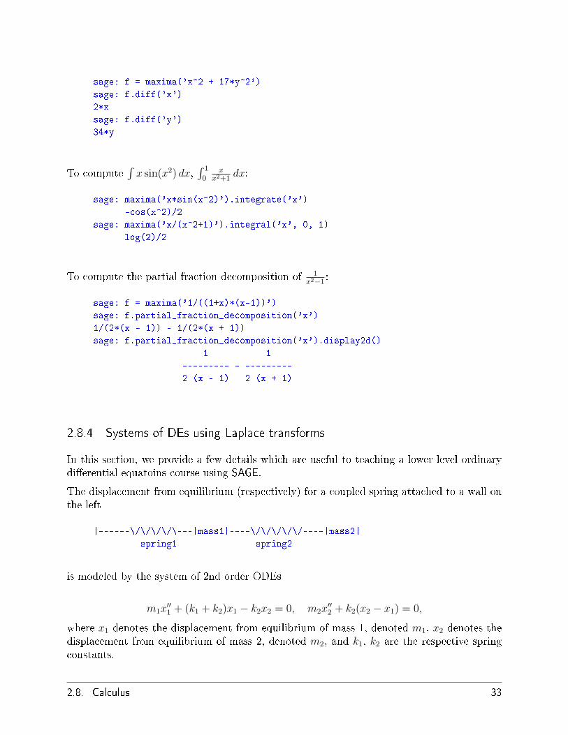
sage: f = maxima('x^2 + 17*y^2')
sage: f.diff('x')
2*x
sage: f.diff('y')
34*y
To compute∫
x sin(x2) dx,∫ 1
0x
x2+1dx:
sage: maxima('x*sin(x^2)').integrate('x')
-cos(x^2)/2
sage: maxima('x/(x^2+1)').integral('x', 0, 1)
log(2)/2
To compute the partial fraction decomposition of 1x2−1
:
sage: f = maxima('1/((1+x)*(x-1))')
sage: f.partial_fraction_decomposition('x')
1/(2*(x - 1)) - 1/(2*(x + 1))
sage: f.partial_fraction_decomposition('x').display2d()
1 1
--------- - ---------
2 (x - 1) 2 (x + 1)
2.8.4 Systems of DEs using Laplace transforms
In this section, we provide a few details which are useful to teaching a lower level ordinarydi�erential equatoins course using SAGE.
The displacement from equilibrium (respectively) for a coupled spring attached to a wall onthe left
|------\/\/\/\/\---|mass1|----\/\/\/\/\/----|mass2|
spring1 spring2
is modeled by the system of 2nd order ODEs
m1x′′1 + (k1 + k2)x1 − k2x2 = 0, m2x
′′2 + k2(x2 − x1) = 0,
where x1 denotes the displacement from equilibrium of mass 1, denoted m1, x2 denotes thedisplacement from equilibrium of mass 2, denoted m2, and k1, k2 are the respective springconstants.
2.8. Calculus 33
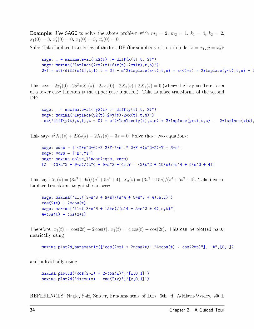
Example: Use SAGE to solve the above problem with m1 = 2, m2 = 1, k1 = 4, k2 = 2,x1(0) = 3, x′1(0) = 0, x2(0) = 3, x′2(0) = 0.
Soln: Take Laplace transforms of the �rst DE (for simplicity of notation, let x = x1, y = x2):
sage: _ = maxima.eval("x2(t) := diff(x(t),t, 2)")
sage: maxima("laplace(2*x2(t)+6*x(t)-2*y(t),t,s)")
2*( - at('diff(x(t),t,1),t = 0) + s^2*laplace(x(t),t,s) - x(0)*s) - 2*laplace(y(t),t,s) + 6*laplace(x(t),t,s)
This says −2x′1(0)+2s2∗X1(s)−2sx1(0)−2X2(s)+2X1(s) = 0 (where the Laplace transformof a lower case function is the upper case function). Take Laplace transforms of the secondDE:
sage: _ = maxima.eval("y2(t) := diff(y(t),t, 2)")
sage: maxima("laplace(y2(t)+2*y(t)-2*x(t),t,s)")
-at('diff(y(t),t,1),t = 0) + s^2*laplace(y(t),t,s) + 2*laplace(y(t),t,s) - 2*laplace(x(t),t,s) - y(0)*s
This says s2X2(s) + 2X2(s)− 2X1(s)− 3s = 0. Solve these two equations:
sage: eqns = ["(2*s^2+6)*X-2*Y=6*s","-2*X +(s^2+2)*Y = 3*s"]
sage: vars = ["X","Y"]
sage: maxima.solve_linear(eqns, vars)
[X = (3*s^3 + 9*s)/(s^4 + 5*s^2 + 4),Y = (3*s^3 + 15*s)/(s^4 + 5*s^2 + 4)]
This says X1(s) = (3s3 +9s)/(s4 +5s2 +4), X2(s) = (3s3 +15s)/(s4 +5s2 +4). Take inverseLaplace transforms to get the answer:
sage: maxima("ilt((3*s^3 + 9*s)/(s^4 + 5*s^2 + 4),s,t)")
cos(2*t) + 2*cos(t)
sage: maxima("ilt((3*s^3 + 15*s)/(s^4 + 5*s^2 + 4),s,t)")
4*cos(t) - cos(2*t)
Therefore, x1(t) = cos(2t) + 2 cos(t), x2(t) = 4 cos(t) − cos(2t). This can be plotted para-metrically using
maxima.plot2d_parametric(["cos(2*t) + 2*cos(t)","4*cos(t) - cos(2*t)"], "t",[0,1])
and individually using
maxima.plot2d('cos(2*x) + 2*cos(x)','[x,0,1]')
maxima.plot2d('4*cos(x) - cos(2*x)','[x,0,1]')
REFERENCES: Nagle, Sa�, Snider, Fundamentals of DEs, 6th ed, Addison-Wesley, 2004.
34 Chapter 2. A Guided Tour

(see �5.5).
2.8.5 Euler's method for systems of DEs
Finally, we show how the �les in the examples/calculus subdirectory of the main SAGE_HOME
directory can be used. (And please feel free to contribute your own by emailing them to theSAGE Forum or to William Stein.)
In the next example, we will illustrate Euler's method for 2nd order ODE's. We �rst recallthe basic idea. The goal is to �nd an approximate solution to the problem
y′ = f(x, y), y(a) = c, (2.1)
where f(x, y) is some given function. We shall try to approximate the value of the solutionat x = b, where b > a is given.
Recall from the de�nition of the derivative that
y′(x) ∼=y(x + h)− y(x)
h,
h > 0 is a given and small. This and the DE together give f(x, y(x)) ∼= y(x+h)−y(x)h
. Nowsolve for y(x + h):
y(x + h) ∼= y(x) + h · f(x, y(x)).
If we call h · f(x, y(x)) the �correction term� (for lack of anything better), call y(x) the �oldvalue of y�, and call y(x+h) the �new value of y�, then this approximation can be re-expressed
ynew = yold + h · f(x, yold).
Tabular idea: Let n > 0 be an integer, which we call the step size. This is related to theincrement by
h =b− a
n.
This can be expressed simplest using a table.
x y hf(x, y)a c hf(a, c)
a + h c + hf(a, c)...
a + 2h...
...b ??? xxx
2.8. Calculus 35
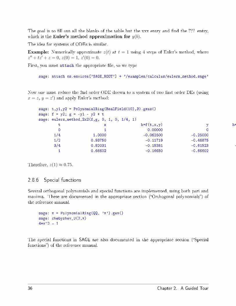
The goal is to �ll out all the blanks of the table but the xxx entry and �nd the ??? entry,which is the Euler's method approximation for y(b).
The idea for systems of ODEs is similar.
Example: Numerically approximate z(t) at t = 1 using 4 steps of Euler's method, wherez′′ + tz′ + z = 0, z(0) = 1, z′(0) = 0.
First, you must attach the appropriate �le, so we type
sage: attach os.environ['SAGE_ROOT'] + '/examples/calculus/eulers_method.sage'
Now one must reduce the 2nd order ODE doewn to a system of two �rst order DEs (usingx = z, y = z′) and apply Euler's method:
sage: t,y1,y2 = PolynomialRing(RealField(10),3).gens()
sage: f = y2; g = -y1 - y2 * t
sage: eulers_method_2x2(f,g, 0, 1, 0, 1/4, 1)
t x h*f(t,x,y) y h*g(t,x,y)
0 1 0.00000 0 -0.25000
1/4 1.0000 -0.062500 -0.25000 -0.23438
1/2 0.93750 -0.11719 -0.46875 -0.17578
3/4 0.82031 -0.15381 -0.61523 -0.089722
1 0.66602 -0.16650 -0.66602 0.00000
Therefore, z(1) ≈ 0.75.
2.8.6 Special functions
Several orthogonal polynomials and special functions are implemented, using both pari andmaxima. These are documented in the appropriate section (�Orthogonal polynomials�) ofthe reference manual.
sage: x = PolynomialRing(QQ, 'x').gen()
sage: chebyshev_U(2,x)
4*x^2 - 1
The special functions in SAGE are also documented in the appropriate section (�Specialfunctions�) of the reference manual.
36 Chapter 2. A Guided Tour

sage: bessel_I(1,1,"pari",500)
0.56515910399248502720769602760986330732889962162109200948029448947925564096437113409266499776681441006467788605552630267685763768491717981204113120812118
sage: bessel_I(1,1)
0.56515910399248503
sage: bessel_I(2,1.1,"maxima") # last few digits are random
0.16708949925104899
Maxima has �xed accuracy, whereas those functions implemented using pari have higheraccuracy.
2.9 Algebraic Geometry
You can de�ne arbitrary algebraic varieties in SAGE, but all too frequently, nontrivial func-tionality is limited to rings over Q or prime �elds. For example, we compute the union oftwo a�ne plane curves, then recover the curves as the irreducible components of the union.
sage: x, y = AffineSpace(2, QQ, 'xy').gens()
sage: C2 = Curve(x^2 + y^2 - 1)
sage: C3 = Curve(x^3 + y^3 - 1)
sage: D = C2 + C3
sage: D
Affine Curve over Rational Field defined by 1 - y^2 - y^3 + y^5 - x^2
+ x^2*y^3 - x^3 + x^3*y^2 + x^5
sage: D.irreducible_components()
[Closed subscheme of Affine Space of dimension 2 over Rational Field defined by:
-1 + y^2 + x^2,
Closed subscheme of Affine Space of dimension 2 over Rational Field defined by:
-1 + y^3 + x^3]
We can also �nd all points of intersection of the two curves by intersecting them and com-puting the irreducible components.
2.9. Algebraic Geometry 37

sage: V = C2.intersection(C3)
sage: V.irreducible_components()
[Closed subscheme of Affine Space of dimension 2 over Rational Field defined by:
y
-1 + x, Closed subscheme of Affine Space of dimension 2 over Rational Field defined by:
x
-1 + y, Closed subscheme of Affine Space of dimension 2 over Rational Field defined by:
2 + y + x
3 + 4*y + 2*y^2]
Thus, e.g., (1, 0) and (0, 1) are on both curves (visibly clear), as are certain (quadratic)points whose y coordinate satisfy 2y2 + 4y + 3 = 0.
2.10 Modular Forms
SAGE can do some computations related to modular forms, including dimensions, computingspaces of modular symbols, Hecke operators, and decompositions.
There are several functions available for computing dimensions of spaces of modular forms.For example,
sage: dimension_cusp_forms(Gamma0(11),2)
1
sage: dimension_cusp_forms(Gamma0(1),12)
1
sage: dimension_cusp_forms(Gamma1(389),2)
6112
Next we illustrate computation of Hecke operators on a space of modular symbols of level 1and weight 12.
38 Chapter 2. A Guided Tour

sage: M = ModularSymbols(1,12)
sage: M.basis()
([X^8*Y^2,(0,0)], [X^9*Y,(0,0)], [X^10,(0,0)])
sage: t2 = M.T(2)
sage: t2
Hecke operator T_2 on Modular Symbols space of dimension 3 for Gamma_0(1) of weight 12 with sign 0 over Rational Field
sage: t2.matrix()
[ -24 0 0]
[ 0 -24 0]
[4860 0 2049]
sage: f = t2.charpoly(); f
x^3 - 2001*x^2 - 97776*x - 1180224
sage: factor(f)
(x - 2049) * (x + 24)^2
sage: M.T(11).charpoly().factor()
(x - 285311670612) * (x - 534612)^2
We can also create spaces for Γ0(N) and Γ1(N).
sage: ModularSymbols(11,2)
Modular Symbols space of dimension 3 for Gamma_0(11) of weight 2 with sign 0 over Rational Field
sage: ModularSymbols(Gamma1(11),2)
Modular Symbols space of dimension 11 for Gamma_1(11) of weight 2 with sign 0 and over Rational Field
Let's compute some characteristic polynomials and q-expansions.
sage: M = ModularSymbols(Gamma1(11),2)
sage: M.T(2).charpoly()
x^11 - 8*x^10 + 20*x^9 + 10*x^8 - 145*x^7 + 229*x^6 + 58*x^5
- 360*x^4 + 70*x^3 - 515*x^2 + 1804*x - 1452
sage: M.T(2).charpoly().factor()
(x - 3) * (x + 2)^2 * (x^4 - 7*x^3 + 19*x^2 - 23*x + 11)
* (x^4 - 2*x^3 + 4*x^2 + 2*x + 11)
sage: S = M.cuspidal_submodule()
sage: S.T(2).matrix()
[-2 0]
[ 0 -2]
sage: S.q_expansion_basis(10)
[
q - 2*q^2 - q^3 + 2*q^4 + q^5 + 2*q^6 - 2*q^7 - 2*q^9 + O(q^10)
]
We can even compute spaces of modular symbols with character.
2.10. Modular Forms 39
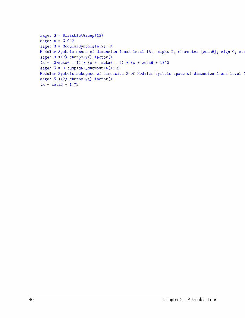
sage: G = DirichletGroup(13)
sage: e = G.0^2
sage: M = ModularSymbols(e,2); M
Modular Symbols space of dimension 4 and level 13, weight 2, character [zeta6], sign 0, over Cyclotomic Field of order 6 and degree 2
sage: M.T(2).charpoly().factor()
(x + -2*zeta6 - 1) * (x + -zeta6 - 2) * (x + zeta6 + 1)^2
sage: S = M.cuspidal_submodule(); S
Modular Symbols subspace of dimension 2 of Modular Symbols space of dimension 4 and level 13, weight 2, character [zeta6], sign 0, over Cyclotomic Field of order 6 and degree 2
sage: S.T(2).charpoly().factor()
(x + zeta6 + 1)^2
40 Chapter 2. A Guided Tour

CHAPTER
THREE
The Interactive Shell
In most of this tutorial we assume you start the SAGE interpreter using the sage command.This starts a customized version of the IPython shell, and imports many functions andclasses, so they are ready to use from the command prompt. Further customization ispossible by editing the $SAGE_ROOT/ipythonrc �le. Upon starting SAGE you get outputsimilar to the following:
--------------------------------------------------------
| SAGE Version 1.0.0.1, Build Date: 2006-02-05-0745 |
| Distributed under the GNU General Public License V2 |
| For help type <object>?, <object>??, %magic, or help |
--------------------------------------------------------
sage:
To quit SAGE either press Ctrl-D or type quit or exit.
sage: quit
Exiting SAGE (CPU time 0m0.00s, Wall time 0m0.89s)
The wall time is the time that elapsed on the clock hanging from your wall. This is relevant,since CPU time does not track time used by subprocesses like Gap or Singular.
Note: Avoid killing a SAGE process with kill -9 from a terminal, since SAGE might notkill child processes, e.g., maple processes, or cleanup tempoary �les from $HOME/.sage/tmp.
3.1 Your SAGE session
The session is the sequence of input and output from when you start SAGE until you quit.SAGE via IPython logs all SAGE input. In fact, at any point, you may type %hist to get alisting of all input lines typed so far. You can type ? at the SAGE prompt to �nd out moreabout IPython, e.g., �IPython o�ers numbered prompts ... with input and output caching.All input is saved and can be retrieved as variables (besides the usual arrow key recall). The
41
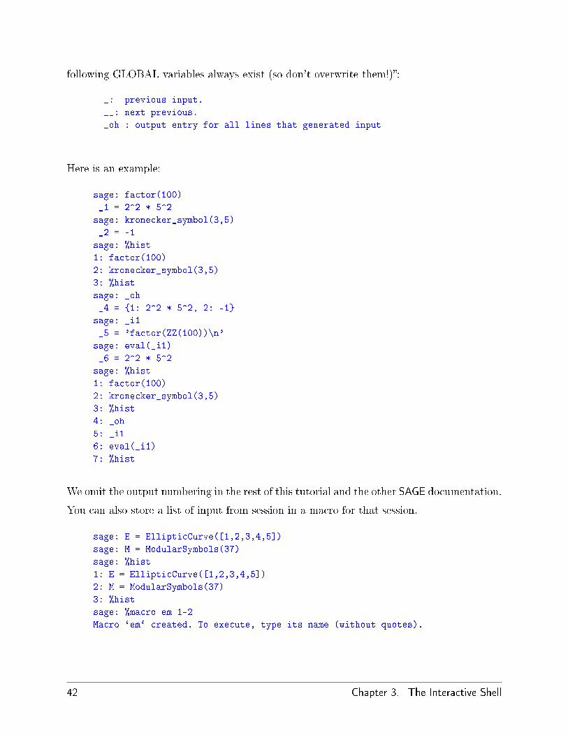
following GLOBAL variables always exist (so don't overwrite them!)�:
_: previous input.
__: next previous.
_oh : output entry for all lines that generated input
Here is an example:
sage: factor(100)
_1 = 2^2 * 5^2
sage: kronecker_symbol(3,5)
_2 = -1
sage: %hist
1: factor(100)
2: kronecker_symbol(3,5)
3: %hist
sage: _oh
_4 = {1: 2^2 * 5^2, 2: -1}
sage: _i1
_5 = 'factor(ZZ(100))\n'
sage: eval(_i1)
_6 = 2^2 * 5^2
sage: %hist
1: factor(100)
2: kronecker_symbol(3,5)
3: %hist
4: _oh
5: _i1
6: eval(_i1)
7: %hist
We omit the output numbering in the rest of this tutorial and the other SAGE documentation.
You can also store a list of input from session in a macro for that session.
sage: E = EllipticCurve([1,2,3,4,5])
sage: M = ModularSymbols(37)
sage: %hist
1: E = EllipticCurve([1,2,3,4,5])
2: M = ModularSymbols(37)
3: %hist
sage: %macro em 1-2
Macro `em` created. To execute, type its name (without quotes).
42 Chapter 3. The Interactive Shell
sage: E
Elliptic Curve defined by y^2 + x*y + 3*y = x^3 + 2*x^2 + 4*x + 5 over Rational Field
sage: E = 5
sage: M = None
sage: em
Executing Macro...
sage: E
Elliptic Curve defined by y^2 + x*y + 3*y = x^3 + 2*x^2 + 4*x + 5 over Rational Field
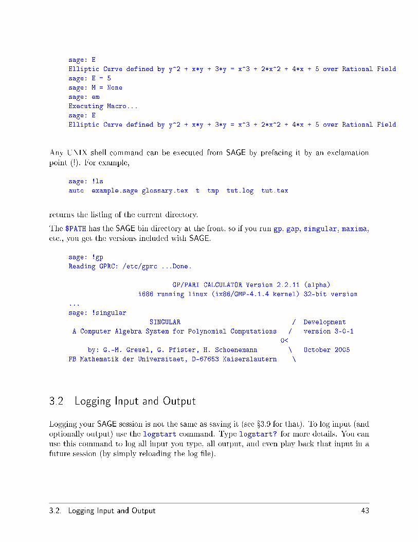
Any UNIX shell command can be executed from SAGE by prefacing it by an exclamationpoint (!). For example,
sage: !ls
auto example.sage glossary.tex t tmp tut.log tut.tex
returns the listing of the current directory.
The $PATH has the SAGE bin directory at the front, so if you run gp, gap, singular, maxima,etc., you get the versions included with SAGE.
sage: !gp
Reading GPRC: /etc/gprc ...Done.
GP/PARI CALCULATOR Version 2.2.11 (alpha)
i686 running linux (ix86/GMP-4.1.4 kernel) 32-bit version
...
sage: !singular
SINGULAR / Development
A Computer Algebra System for Polynomial Computations / version 3-0-1
0<
by: G.-M. Greuel, G. Pfister, H. Schoenemann \ October 2005
FB Mathematik der Universitaet, D-67653 Kaiserslautern \
3.2 Logging Input and Output
Logging your SAGE session is not the same as saving it (see �3.9 for that). To log input (andoptionally output) use the logstart command. Type logstart? for more details. You canuse this command to log all input you type, all output, and even play back that input in afuture session (by simply reloading the log �le).
3.2. Logging Input and Output 43

was@form:~$ sage
--------------------------------------------------------
| SAGE Version 0.10.11, Build Date: 2006-01-28-0723 |
| Distributed under the GNU General Public License V2 |
| For help type <object>?, <object>??, %magic, or help |
--------------------------------------------------------
sage: logstart setup
Activating auto-logging. Current session state plus future input saved.
Filename : setup
Mode : backup
Output logging : False
Timestamping : False
State : active
sage: E = EllipticCurve([1,2,3,4,5]).minimal_model()
sage: F = QQ^3
sage: x,y = QQ['x,y'].gens()
sage: G = E.gens()
sage:
Exiting SAGE (CPU time 0m0.61s, Wall time 0m50.39s).
was@form:~$ sage
--------------------------------------------------------
| SAGE Version 0.10.11, Build Date: 2006-01-28-0723 |
| Distributed under the GNU General Public License V2 |
| For help type <object>?, <object>??, %magic, or help |
--------------------------------------------------------
sage: load "setup"
Loading log file <setup> one line at a time...
Finished replaying log file <setup>
sage: E
Elliptic Curve defined by y^2 + x*y = x^3 - x^2 + 4*x + 3 over Rational Field
sage: x*y
x*y
sage: G
[(2 : 3 : 1)]
If you use SAGE in the KDE terminal �konsole� then you can save your session as follows:after starting SAGE in konsole, select �settings�, then �history...�, then �set unlimited�. Whenyou are ready to save your session, select �edit� then �save history as...� and type in a nameto save the text of your session to your computer. After saving this �le, you could then loadit into an editor, such as xemacs, and print it.
44 Chapter 3. The Interactive Shell

3.3 Paste Ignores Prompts
Suppose you are reading a session of SAGE or Python computations and want to copy theminto SAGE. But there are annoying >>> or sage: prompts to worry about. In fact, you cancopy and paste an example, including the prompts if you want, into SAGE. In other words,by default the SAGE parser strips any leading >>> or sage: prompt before passing it toPython. For example,
sage: 2^10
1024
sage: sage: sage: 2^10
1024
sage: >>> 2^10
1024
3.4 Timing Commands
If you place the time command at the beginning of an input line, the time the commandtakes to run will be displayed after the output. For example, we can compare the runningtime for a certain exponentiation operation in several ways. The timings below will probablybe much di�erent on your computer, or even between di�erent versions of SAGE. First, nativePython:
sage: time a = int(1938)^int(99484)
CPU times: user 0.66 s, sys: 0.00 s, total: 0.66 s
Wall time: 0.66
This means that 0.66 seconds total were taken, and the �Wall time�, i.e., the amount of timethat elapsed on your wall clock, is also 0.66 seconds. If your computer is heavily loaded withother programs the wall time may be much larger than the CPU time.
Next we time exponentiation using the native SAGE Integer type, which is implemented (inPyrex) using the GMP library:
sage: time a = 1938^99484
CPU times: user 0.04 s, sys: 0.00 s, total: 0.04 s
Wall time: 0.04
Using the PARI C-library interface:
3.3. Paste Ignores Prompts 45

sage: time a = pari(1938)^pari(99484)
CPU times: user 0.05 s, sys: 0.00 s, total: 0.05 s
Wall time: 0.05
GMP is better, but only slightly (as expected, since the version of PARI built for SAGE usesGMP for integer arithmetic).
You can also time a block of commands using the cputime command, as illustrated below:
sage: t = cputime()
sage: a = int(1938)^int(99484)
sage: b = 1938^99484
sage: c = pari(1938)^pari(99484)
sage: cputime(t) # somewhat random output
0.64
sage: cputime?
...
Return the time in CPU second since SAGE started, or with optional
argument t, return the time since time t.
INPUT:
t -- (optional) float, time in CPU seconds
OUTPUT:
float -- time in CPU seconds
The walltime command behaves just like the cputime command, except that it measureswall time.
We can also compute the above power in some of the computer algebra systems that SAGEincludes. In each case we execute a trivial command in the system, in order to start upthe server for that program. The most relavant time is the wall time. However, if thereis a signi�cant di�erence between the wall time and the cpu time then this may indicate aperformanve issue worth looking into.
46 Chapter 3. The Interactive Shell
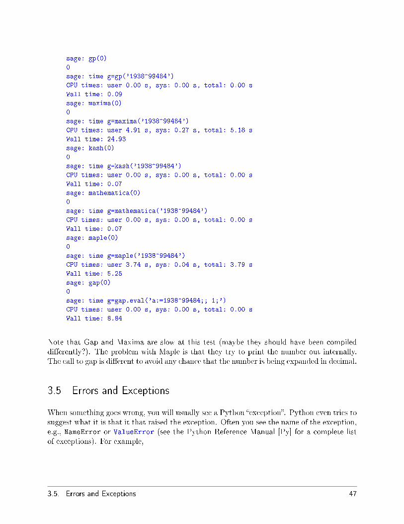
sage: gp(0)
0
sage: time g=gp('1938^99484')
CPU times: user 0.00 s, sys: 0.00 s, total: 0.00 s
Wall time: 0.09
sage: maxima(0)
0
sage: time g=maxima('1938^99484')
CPU times: user 4.91 s, sys: 0.27 s, total: 5.18 s
Wall time: 24.93
sage: kash(0)
0
sage: time g=kash('1938^99484')
CPU times: user 0.00 s, sys: 0.00 s, total: 0.00 s
Wall time: 0.07
sage: mathematica(0)
0
sage: time g=mathematica('1938^99484')
CPU times: user 0.00 s, sys: 0.00 s, total: 0.00 s
Wall time: 0.07
sage: maple(0)
0
sage: time g=maple('1938^99484')
CPU times: user 3.74 s, sys: 0.04 s, total: 3.79 s
Wall time: 5.25
sage: gap(0)
0
sage: time g=gap.eval('a:=1938^99484;; 1;')
CPU times: user 0.00 s, sys: 0.00 s, total: 0.00 s
Wall time: 8.84
Note that Gap and Maxima are slow at this test (maybe they should have been compileddi�erently?). The problem with Maple is that they try to print the number out internally.The call to gap is di�erent to avoid any chance that the number is being expanded in decimal.
3.5 Errors and Exceptions
When something goes wrong, you will usually see a Python �exception�. Python even tries tosuggest what it is that it that raised the exception. Often you see the name of the exception,e.g., NameError or ValueError (see the Python Reference Manual [Py] for a complete listof exceptions). For example,
3.5. Errors and Exceptions 47
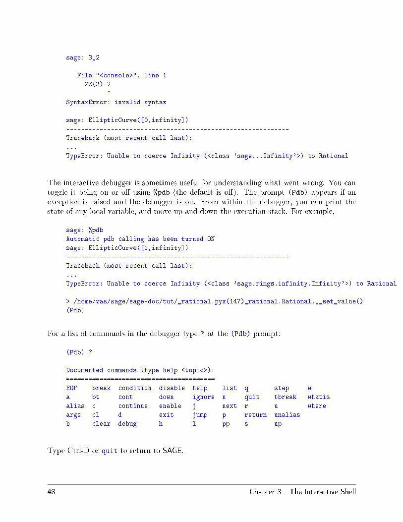
sage: 3_2
------------------------------------------------------------
File "<console>", line 1
ZZ(3)_2
^
SyntaxError: invalid syntax
sage: EllipticCurve([0,infinity])
------------------------------------------------------------
Traceback (most recent call last):
...
TypeError: Unable to coerce Infinity (<class 'sage...Infinity'>) to Rational
The interactive debugger is sometimes useful for understanding what went wrong. You cantoggle it being on or o� using %pdb (the default is o�). The prompt (Pdb) appears if anexception is raised and the debugger is on. From within the debugger, you can print thestate of any local variable, and move up and down the execution stack. For example,
sage: %pdb
Automatic pdb calling has been turned ON
sage: EllipticCurve([1,infinity])
------------------------------------------------------------
Traceback (most recent call last):
...
TypeError: Unable to coerce Infinity (<class 'sage.rings.infinity.Infinity'>) to Rational
> /home/was/sage/sage-doc/tut/_rational.pyx(147)_rational.Rational.__set_value()
(Pdb)
For a list of commands in the debugger type ? at the (Pdb) prompt:
(Pdb) ?
Documented commands (type help <topic>):
========================================
EOF break condition disable help list q step w
a bt cont down ignore n quit tbreak whatis
alias c continue enable j next r u where
args cl d exit jump p return unalias
b clear debug h l pp s up
Type Ctrl-D or quit to return to SAGE.
48 Chapter 3. The Interactive Shell
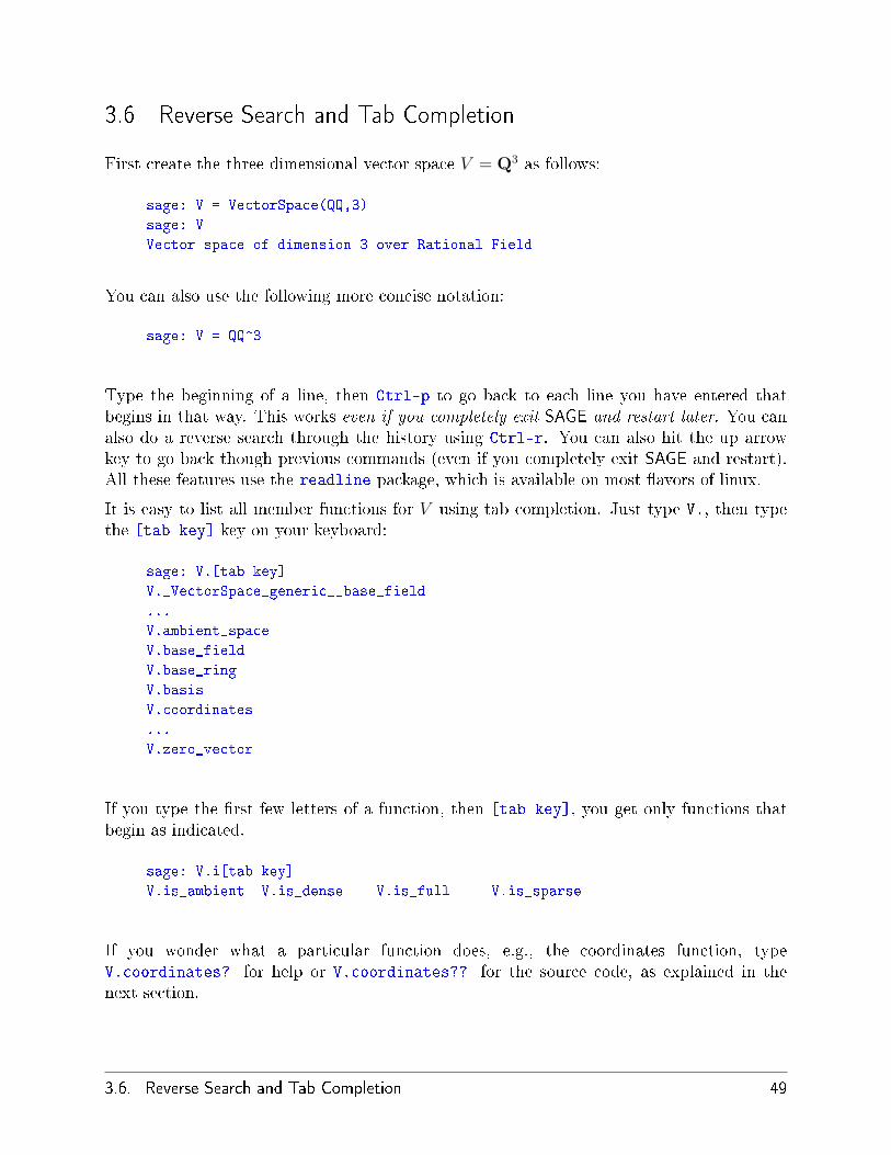
3.6 Reverse Search and Tab Completion
First create the three dimensional vector space V = Q3 as follows:
sage: V = VectorSpace(QQ,3)
sage: V
Vector space of dimension 3 over Rational Field
You can also use the following more concise notation:
sage: V = QQ^3
Type the beginning of a line, then Ctrl-p to go back to each line you have entered thatbegins in that way. This works even if you completely exit SAGE and restart later. You canalso do a reverse search through the history using Ctrl-r. You can also hit the up arrowkey to go back though previous commands (even if you completely exit SAGE and restart).All these features use the readline package, which is available on most �avors of linux.
It is easy to list all member functions for V using tab completion. Just type V., then typethe [tab key] key on your keyboard:
sage: V.[tab key]
V._VectorSpace_generic__base_field
...
V.ambient_space
V.base_field
V.base_ring
V.basis
V.coordinates
...
V.zero_vector
If you type the �rst few letters of a function, then [tab key], you get only functions thatbegin as indicated.
sage: V.i[tab key]
V.is_ambient V.is_dense V.is_full V.is_sparse
If you wonder what a particular function does, e.g., the coordinates function, typeV.coordinates? for help or V.coordinates?? for the source code, as explained in thenext section.
3.6. Reverse Search and Tab Completion 49
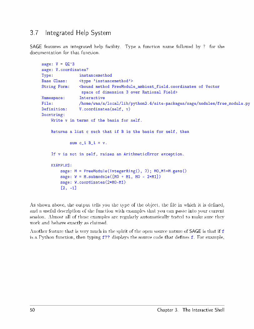
3.7 Integrated Help System
SAGE features an integrated help facility. Type a function name followed by ? for thedocumentation for that function.
sage: V = QQ^3
sage: V.coordinates?
Type: instancemethod
Base Class: <type 'instancemethod'>
String Form: <bound method FreeModule_ambient_field.coordinates of Vector
space of dimension 3 over Rational Field>
Namespace: Interactive
File: /home/was/s/local/lib/python2.4/site-packages/sage/modules/free_module.py
Definition: V.coordinates(self, v)
Docstring:
Write v in terms of the basis for self.
Returns a list c such that if B is the basis for self, then
sum c_i B_i = v.
If v is not in self, raises an ArithmeticError exception.
EXAMPLES:
sage: M = FreeModule(IntegerRing(), 2); M0,M1=M.gens()
sage: W = M.submodule([M0 + M1, M0 - 2*M1])
sage: W.coordinates(2*M0-M1)
[2, -1]
As shown above, the output tells you the type of the object, the �le in which it is de�ned,and a useful description of the function with examples that you can paste into your currentsession. Almost all of these examples are regularly automatically tested to make sure theywork and behave exactly as claimed.
Another feature that is very much in the spirit of the open source nature of SAGE is that if fis a Python function, then typing f?? displays the source code that de�nes f. For example,
50 Chapter 3. The Interactive Shell
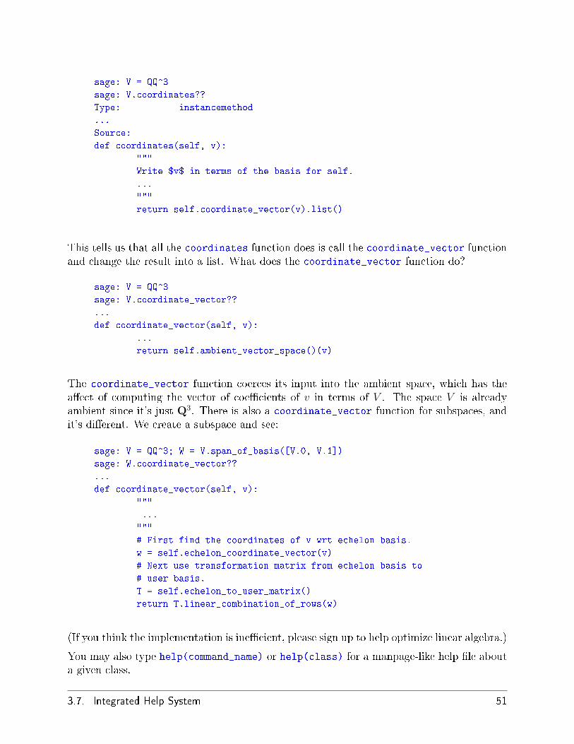
sage: V = QQ^3
sage: V.coordinates??
Type: instancemethod
...
Source:
def coordinates(self, v):
"""
Write $v$ in terms of the basis for self.
...
"""
return self.coordinate_vector(v).list()
This tells us that all the coordinates function does is call the coordinate_vector functionand change the result into a list. What does the coordinate_vector function do?
sage: V = QQ^3
sage: V.coordinate_vector??
...
def coordinate_vector(self, v):
...
return self.ambient_vector_space()(v)
The coordinate_vector function coerces its input into the ambient space, which has thea�ect of computing the vector of coe�cients of v in terms of V . The space V is alreadyambient since it's just Q3. There is also a coordinate_vector function for subspaces, andit's di�erent. We create a subspace and see:
sage: V = QQ^3; W = V.span_of_basis([V.0, V.1])
sage: W.coordinate_vector??
...
def coordinate_vector(self, v):
"""
...
"""
# First find the coordinates of v wrt echelon basis.
w = self.echelon_coordinate_vector(v)
# Next use transformation matrix from echelon basis to
# user basis.
T = self.echelon_to_user_matrix()
return T.linear_combination_of_rows(w)
(If you think the implementation is ine�cient, please sign up to help optimize linear algebra.)
You may also type help(command_name) or help(class) for a manpage-like help �le abouta given class.
3.7. Integrated Help System 51
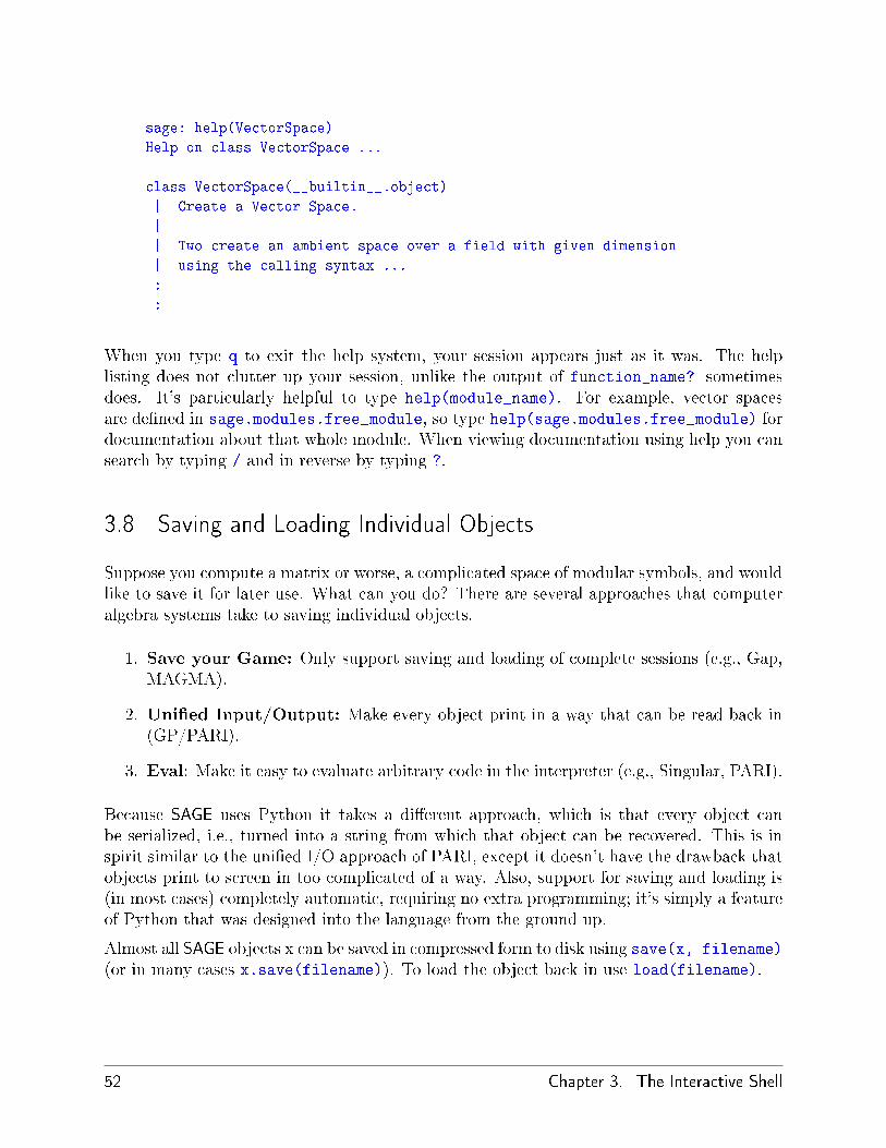
sage: help(VectorSpace)
Help on class VectorSpace ...
class VectorSpace(__builtin__.object)
| Create a Vector Space.
|
| Two create an ambient space over a field with given dimension
| using the calling syntax ...
:
:
When you type q to exit the help system, your session appears just as it was. The helplisting does not clutter up your session, unlike the output of function_name? sometimesdoes. It's particularly helpful to type help(module_name). For example, vector spacesare de�ned in sage.modules.free_module, so type help(sage.modules.free_module) fordocumentation about that whole module. When viewing documentation using help you cansearch by typing / and in reverse by typing ?.
3.8 Saving and Loading Individual Objects
Suppose you compute a matrix or worse, a complicated space of modular symbols, and wouldlike to save it for later use. What can you do? There are several approaches that computeralgebra systems take to saving individual objects.
1. Save your Game: Only support saving and loading of complete sessions (e.g., Gap,MAGMA).
2. Uni�ed Input/Output: Make every object print in a way that can be read back in(GP/PARI).
3. Eval: Make it easy to evaluate arbitrary code in the interpreter (e.g., Singular, PARI).
Because SAGE uses Python it takes a di�erent approach, which is that every object canbe serialized, i.e., turned into a string from which that object can be recovered. This is inspirit similar to the uni�ed I/O approach of PARI, except it doesn't have the drawback thatobjects print to screen in too complicated of a way. Also, support for saving and loading is(in most cases) completely automatic, requiring no extra programming; it's simply a featureof Python that was designed into the language from the ground up.
Almost all SAGE objects x can be saved in compressed form to disk using save(x, filename)
(or in many cases x.save(filename)). To load the object back in use load(filename).
52 Chapter 3. The Interactive Shell
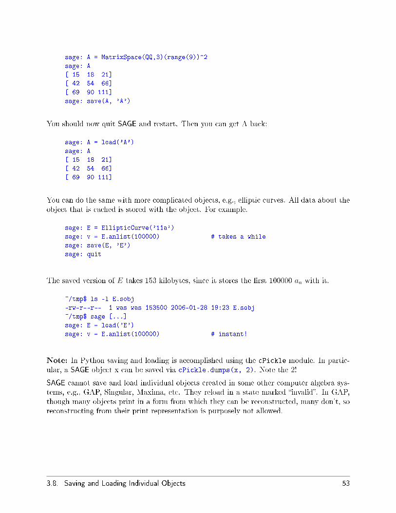
sage: A = MatrixSpace(QQ,3)(range(9))^2
sage: A
[ 15 18 21]
[ 42 54 66]
[ 69 90 111]
sage: save(A, 'A')
You should now quit SAGE and restart. Then you can get A back:
sage: A = load('A')
sage: A
[ 15 18 21]
[ 42 54 66]
[ 69 90 111]
You can do the same with more complicated objects, e.g., elliptic curves. All data about theobject that is cached is stored with the object. For example,
sage: E = EllipticCurve('11a')
sage: v = E.anlist(100000) # takes a while
sage: save(E, 'E')
sage: quit
The saved version of E takes 153 kilobytes, since it stores the �rst 100000 an with it.
~/tmp$ ls -l E.sobj
-rw-r--r-- 1 was was 153500 2006-01-28 19:23 E.sobj
~/tmp$ sage [...]
sage: E = load('E')
sage: v = E.anlist(100000) # instant!
Note: In Python saving and loading is accomplished using the cPickle module. In partic-ular, a SAGE object x can be saved via cPickle.dumps(x, 2). Note the 2!
SAGE cannot save and load individual objects created in some other computer algebra sys-tems, e.g., GAP, Singular, Maxima, etc. They reload in a state marked �invalid�. In GAP,though many objects print in a form from which they can be reconstructed, many don't, soreconstructing from their print representation is purposely not allowed.
3.8. Saving and Loading Individual Objects 53
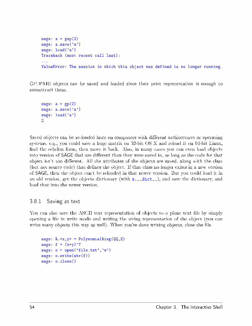
sage: a = gap(2)
sage: a.save('a')
sage: load('a')
Traceback (most recent call last):
...
ValueError: The session in which this object was defined is no longer running.
GP/PARI objects can be saved and loaded since their print representation is enough toreconstruct them.
sage: a = gp(2)
sage: a.save('a')
sage: load('a')
2
Saved objects can be re-loaded later on computers with di�erent architectures or operatingsystems, e.g., you could save a huge matrix on 32-bit OS X and reload it on 64-bit Linux,�nd the echelon form, then move it back. Also, in many cases you can even load objectsinto version of SAGE that are di�erent than they were saved in, as long as the code for thatobject isn't too di�erent. All the attributes of the objects are saved, along with the class(but not source code) that de�nes the object. If that class no longer exists in a new versionof SAGE, then the object can't be reloaded in that newer version. But you could load it inan old version, get the objects dictionary (with x.__dict__), and save the dictionary, andload that into the newer version.
3.8.1 Saving as text
You can also save the ASCII text representation of objects to a plane text �le by simplyopening a �le in write mode and writing the string representation of the object (you canwrite many objects this way as well). When you're done writing objects, close the �le.
sage: R.<x,y> = PolynomialRing(QQ,2)
sage: f = (x+y)^7
sage: o = open('file.txt','w')
sage: o.write(str(f))
sage: o.close()
54 Chapter 3. The Interactive Shell

3.9 Saving and Loading Complete Sessions
SAGE has very �exible support for saving and loading complete sessions.
The command save_session(sessionname) saves all the variables you've de�ned in thecurrent session as a dictionary in the given sessionname. (In the rare case when a variabledoes not support saving, it is simply not saved to the dictionary.) The resulting �le is an.sobj �le and can be loading just like any other object that was saved. When you loadthe objects saved in a session, you get a dictionary whose keys are the variables names andwhose values are the objects.
You can use the load_session(sessionname) command to load the variables de�ned insessionname into the current session. Note that this does not wipe out variables you'vealready de�ned in your current session; instead, the two sessions are merged.
First we start SAGE and de�ne some variables.
~/tmp$ sage
sage: E = EllipticCurve('11a')
sage: M = ModularSymbols(37)
sage: a = 389
sage: t = M.T(2003).matrix(); t.charpoly().factor()
_4 = (x - 2004) * (x - 12)^2 * (x + 54)^2
Next we save our session, which saves each of the above variables into a �le. Then we viewthe �le, which is about 3K in size.
sage: save_session('misc')
Saving a
Saving M
Saving t
Saving E
sage: quit
was@form:~/tmp$ ls -l misc.sobj
-rw-r--r-- 1 was was 2979 2006-01-28 19:47 misc.sobj
Finally we restart SAGE, de�ne an extra variable, and load our saved session.
3.9. Saving and Loading Complete Sessions 55

~/tmp$ sage
[...]
sage: b = 19
sage: load_session('misc')
Loading a
Loading M
Loading E
Loading t
Each saved variable is again available. Moreover, the variable b was not overwritten.
sage: M
Full Modular Symbols space for Gamma_0(37) of weight 2 with sign 0
and dimension 5 over Rational Field
sage: E
Elliptic Curve defined by y^2 + y = x^3 - x^2 - 10*x - 20 over Rational Field
sage: b
19
sage: a
389
3.10 The Notebook Interface
This section is based on a talk "The SAGE notebook interface" by William Stein, SAGEseminar, 6-9-2006 (notes by D. Joyner).
The SAGE notebook is run by typing
sage: notebook()
on the command line of SAGE. Other options are:
�sage: notebook("My worksheet")
which (a) starts a new worksheet (as opposed to the default behaviour of loading thepreviously used worksheet) and (b) places the banner "My worksheet" at the top ofthe page. (It does not name or save your worksheet into a �le though.)
56 Chapter 3. The Interactive Shell
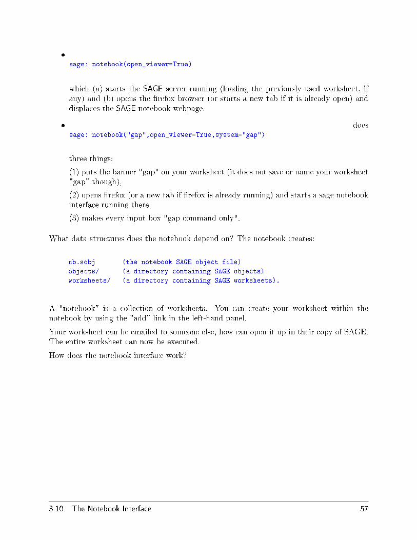
�sage: notebook(open_viewer=True)
which (a) starts the SAGE server running (loading the previously used worksheet, ifany) and (b) opens the �refox browser (or starts a new tab if it is already open) anddisplaces the SAGE notebook webpage.
�sage: notebook("gap",open_viewer=True,system="gap")
does
three things:
(1) puts the banner "gap" on your worksheet (it does not save or name your worksheet"gap" though),
(2) opens �refox (or a new tab if �refox is already running) and starts a sage notebookinterface running there,
(3) makes every input box "gap command only".
What data structures does the notebook depend on? The notebook creates:
nb.sobj (the notebook SAGE object file)
objects/ (a directory containing SAGE objects)
worksheets/ (a directory containing SAGE worksheets).
A "notebook" is a collection of worksheets. You can create your worksheet within thenotebook by using the "add" link in the left-hand panel.
Your worksheet can be emailed to someone else, how can open it up in their copy of SAGE.The entire worksheet can now be executed.
How does the notebook interface work?
3.10. The Notebook Interface 57

----------------------
| |
| |
| firefox |
| |
| javascript |
| program |
| |
| |
----------------------
| ^
| AJAX |
V |
----------------------
| |
| web | SAGE process 1
| | ------------> SAGE process 2 (Python processes)
| server | pexpect SAGE process 3
| | .
| | .
---------------------- .
For help on a SAGE command, <cmd>, in the notebook browser box, type "<cmd>?" andnow hit <esc> (not <shift-enter>).
58 Chapter 3. The Interactive Shell

CHAPTER
FOUR
Interfaces
A central facet of SAGE is that it supports computation with objects in many di�erentcomputer algebra systems �under one roof� using a common interface and clean programminglanguage.
The console and interact methods of an interface do very di�erent things. For example, usinggap as an example:
1. gap.console(): You are completely using another program, e.g., gap/magma/gp HereSAGE is serving as nothing more than a convenient program launcher, similar to bash.
2. gap.interact(): This is a convenient way to interact with a running gap instancethat may be "full of" SAGE objects. You can import SAGE objects into this gap(even from the interactive interface), etc.
4.1 GP/PARI
PARI is a compact, very mature, highly optimized C program whose primary focus is numbertheory. There are two very distinct interfaces that you can use in SAGE:
� gp � the �Go PARI� interpreter, and
� pari � the PARI C library.
For example, the following are two ways of doing the same thing. They look identical, butthe output is actually di�erent, and what happens behind the scenes is drastically di�erent.
sage: gp('znprimroot(10007)')
Mod(5, 10007)
sage: pari('znprimroot(10007)')
Mod(5, 10007)
In the �rst case a separate copy of the GP interepreter is started as a server, and the string
59

'znprimroot(10007)' is sent to it, evaluated by GP, and the result is assigned to a variablein GP (which takes up space in the child GP processes memory that won't be freed). Thenthe value of that variable is displayed. In the second case, no separate program is started,and the string 'znprimroot(10007)' is evaluated by a certain PARI C library function. Theresult is stored in a piece of memory on the Python heap, which is freed when the variableis no longer referenced. The objects have di�erent types:
sage: type(gp('znprimroot(10007)'))
<class 'sage.interfaces.gp.GpElement'>
sage: type(pari('znprimroot(10007)'))
<type 'gen.gen'>
So which should you use? It depends on what you're doing. The GP interface can doabsolutely anything you could do in the usual GP/PARI command line program, since itis running that program. In particular, you can load complicated PARI programs and runthem. In contrast, the PARI interface (via the C library) is much more restrictive; �rstnot all member functions have been implemented. Second; a lot of code, e.g., involvingnumerical integration, won't work via the PARI interface. That said, the PARI interface canbe signi�cantly faster and more robust then the GP one.
Note: If the GP interface runs out of memory evaluating a given input line, it will silentlyand automatically double the stack size and retry that input line. Thus your computationwon't crash if you didn't correctly anticipate the amount of memory that would be needed.This is a nice trick the usual GP interpreter doesn't seem to provide. Regarding the PARIC-library interface, it immediately copies each created object o� of the PARI stack, hencethe stack never grows. However, each object must not exceed 100MB in size, or the stackwill over�ow when the object is being created. This extra copying does impose a slightperformance penalty.
In summary, SAGE uses the PARI C library to provide functionality similar to that providedby the GP/PARI interpreter, except with di�erent sophisticated memory management andthe Python programming language.
First we create a PARI list from a Python list.
sage: v = pari([1,2,3,4,5])
sage: v
[1, 2, 3, 4, 5]
sage: type(v)
<type 'gen.gen'>
Every PARI object is of type py_pari.gen. The PARI type of the underlying object can beobtained using the type member function.
60 Chapter 4. Interfaces
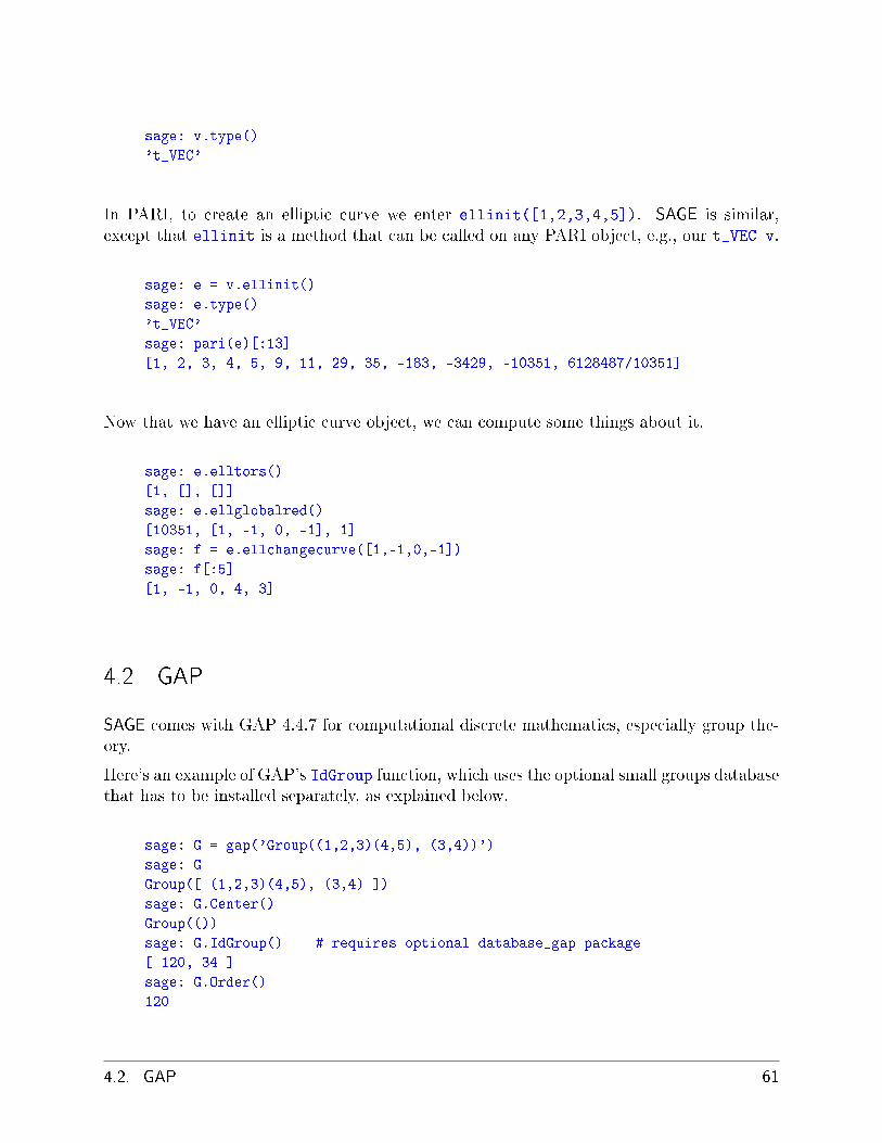
sage: v.type()
't_VEC'
In PARI, to create an elliptic curve we enter ellinit([1,2,3,4,5]). SAGE is similar,except that ellinit is a method that can be called on any PARI object, e.g., our t_VEC v.
sage: e = v.ellinit()
sage: e.type()
't_VEC'
sage: pari(e)[:13]
[1, 2, 3, 4, 5, 9, 11, 29, 35, -183, -3429, -10351, 6128487/10351]
Now that we have an elliptic curve object, we can compute some things about it.
sage: e.elltors()
[1, [], []]
sage: e.ellglobalred()
[10351, [1, -1, 0, -1], 1]
sage: f = e.ellchangecurve([1,-1,0,-1])
sage: f[:5]
[1, -1, 0, 4, 3]
4.2 GAP
SAGE comes with GAP 4.4.7 for computational discrete mathematics, especially group the-ory.
Here's an example of GAP's IdGroup function, which uses the optional small groups databasethat has to be installed separately, as explained below.
sage: G = gap('Group((1,2,3)(4,5), (3,4))')
sage: G
Group([ (1,2,3)(4,5), (3,4) ])
sage: G.Center()
Group(())
sage: G.IdGroup() # requires optional database_gap package
[ 120, 34 ]
sage: G.Order()
120
4.2. GAP 61

We can do the same computation in SAGE without explicitly invoking the GAP interface asfollows:
sage: G = PermutationGroup([[(1,2,3),(4,5)],[(3,4)]])
sage: G.center()
Permutation Group with generators [()]
sage: G.group_id() # requires optional database_gap package
[120, 34]
sage: n = G.order(); n
120
Note: For some GAP functionality, you should install two optional SAGE packages. Typesage -optional for a list and choose the one that looks like gap_packages-x.y.z, then typesage -i gap_packages-x.y.z. Do the same for database_gap-x.y.z. Some non-GPL'dGAP packages may be installed by downloading them from the GAP web site [GAPkg], andunpacking them in $SAGE_ROOT/local/lib/gap-4.4.7/pkg.
4.3 Singular
Singular provides a massive and mature library for Gröbner bases, multivariate polynomialgcds, bases of Riemann-Roch spaces of a plane curve, and factorizations, among other things.We illustrate multivariate polynomial factorization using the SAGE interface to Singular:
sage: R1 = singular.ring(0, '(x,y)', 'dp')
sage: R1
// characteristic : 0
// number of vars : 2
// block 1 : ordering dp
// : names x y
// block 2 : ordering C
sage: f = singular('9*y^8 - 9*x^2*y^7 - 18*x^3*y^6 - 18*x^5*y^6 + 9*x^6*y^4 + 18*x^7*y^5 + 36*x^8*y^4 + 9*x^10*y^4 - 18*x^11*y^2 - 9*x^12*y^3 - 18*x^13*y^2 + 9*x^16')
Now that we have de�ned f , we print it and factor.
62 Chapter 4. Interfaces
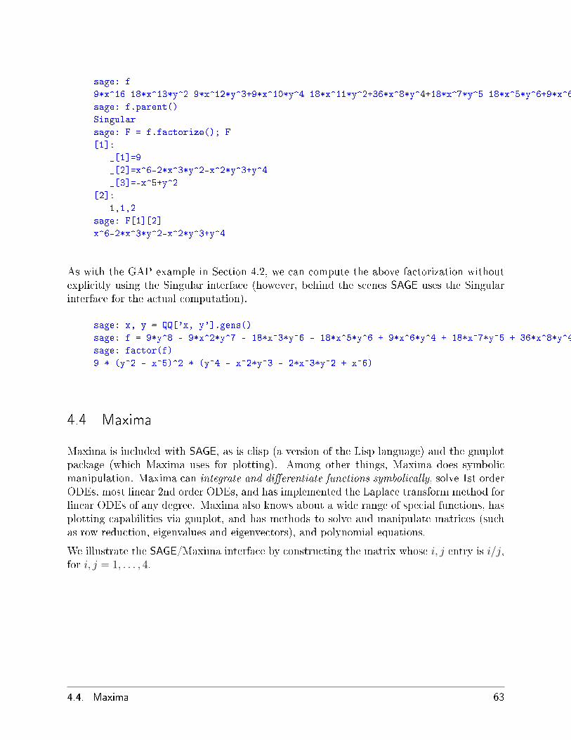
sage: f
9*x^16-18*x^13*y^2-9*x^12*y^3+9*x^10*y^4-18*x^11*y^2+36*x^8*y^4+18*x^7*y^5-18*x^5*y^6+9*x^6*y^4-18*x^3*y^6-9*x^2*y^7+9*y^8
sage: f.parent()
Singular
sage: F = f.factorize(); F
[1]:
_[1]=9
_[2]=x^6-2*x^3*y^2-x^2*y^3+y^4
_[3]=-x^5+y^2
[2]:
1,1,2
sage: F[1][2]
x^6-2*x^3*y^2-x^2*y^3+y^4
As with the GAP example in Section 4.2, we can compute the above factorization withoutexplicitly using the Singular interface (however, behind the scenes SAGE uses the Singularinterface for the actual computation).
sage: x, y = QQ['x, y'].gens()
sage: f = 9*y^8 - 9*x^2*y^7 - 18*x^3*y^6 - 18*x^5*y^6 + 9*x^6*y^4 + 18*x^7*y^5 + 36*x^8*y^4 + 9*x^10*y^4 - 18*x^11*y^2 - 9*x^12*y^3 - 18*x^13*y^2 + 9*x^16
sage: factor(f)
9 * (y^2 - x^5)^2 * (y^4 - x^2*y^3 - 2*x^3*y^2 + x^6)
4.4 Maxima
Maxima is included with SAGE, as is clisp (a version of the Lisp language) and the gnuplotpackage (which Maxima uses for plotting). Among other things, Maxima does symbolicmanipulation. Maxima can integrate and di�erentiate functions symbolically, solve 1st orderODEs, most linear 2nd order ODEs, and has implemented the Laplace transform method forlinear ODEs of any degree. Maxima also knows about a wide range of special functions, hasplotting capabilities via gnuplot, and has methods to solve and manipulate matrices (suchas row reduction, eigenvalues and eigenvectors), and polynomial equations.
We illustrate the SAGE/Maxima interface by constructing the matrix whose i, j entry is i/j,for i, j = 1, . . . , 4.
4.4. Maxima 63
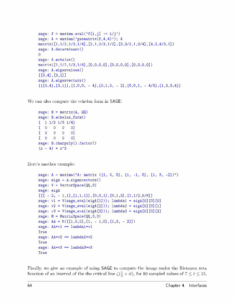
sage: f = maxima.eval('f[i,j] := i/j')
sage: A = maxima('genmatrix(f,4,4)'); A
matrix([1,1/2,1/3,1/4],[2,1,2/3,1/2],[3,3/2,1,3/4],[4,2,4/3,1])
sage: A.determinant()
0
sage: A.echelon()
matrix([1,1/2,1/3,1/4],[0,0,0,0],[0,0,0,0],[0,0,0,0])
sage: A.eigenvalues()
[[0,4],[3,1]]
sage: A.eigenvectors()
[[[0,4],[3,1]],[1,0,0, - 4],[0,1,0, - 2],[0,0,1, - 4/3],[1,2,3,4]]
We can also compute the echelon form in SAGE:
sage: B = matrix(A, QQ)
sage: B.echelon_form()
[ 1 1/2 1/3 1/4]
[ 0 0 0 0]
[ 0 0 0 0]
[ 0 0 0 0]
sage: B.charpoly().factor()
(x - 4) * x^3
Here's another example:
sage: A = maxima("A: matrix ([1, 0, 0], [1, -1, 0], [1, 3, -2])")
sage: eigA = A.eigenvectors()
sage: V = VectorSpace(QQ,3)
sage: eigA
[[[ - 2, - 1,1],[1,1,1]],[0,0,1],[0,1,3],[1,1/2,5/6]]
sage: v1 = V(sage_eval(eigA[1])); lambda1 = eigA[0][0][0]
sage: v2 = V(sage_eval(eigA[2])); lambda2 = eigA[0][0][1]
sage: v3 = V(sage_eval(eigA[3])); lambda3 = eigA[0][0][2]
sage: M = MatrixSpace(QQ,3,3)
sage: AA = M([[1,0,0],[1, - 1,0],[1,3, - 2]])
sage: AA*v1 == lambda1*v1
True
sage: AA*v2 == lambda2*v2
True
sage: AA*v3 == lambda3*v3
True
Finally, we give an example of using SAGE to compute the image under the Riemann zetafunction of an interval of the the critical line ζ(1
2+ it), for 80 sampled values of 7 ≤ t ≤ 15,
64 Chapter 4. Interfaces

saving the real and imaginary points into lists, then using Maxima (which calls gnuplot) toplot these points and save the resulting graph into the current directory.
sage: Z = [ (1/2 + n*I/10).zeta() for n in range(70,150) ]
sage: Z_x = [w.real() for w in Z]
sage: Z_y = [w.imag() for w in Z]
We �rst make the graph appear in a pop-up window.
sage: maxima.plot_list(Z_x, Z_y)
We can also save the graph a �le.
sage: opts='[gnuplot_preamble, "set nokey"], [gnuplot_term, ps], [gnuplot_out_file, "zeta.eps"]'
sage: maxima.plot_list(Z_x, Z_y, opts)
4.4. Maxima 65

66

CHAPTER
FIVE
Programming
5.1 Loading and Attaching SAGE �les
Next we illustrate how to load programs written in a separate �le into SAGE. Create a �lecalled example.sage with the following content:
print "Hello World"
print 2^3
You can read in and execute example.sage �le using the load command.
sage: load "example.sage"
Hello World
8
You can also attach a SAGE �le to a running session using the attach command:
sage: attach "example.sage"
Hello World
8
Now if you change example.sage and enter one blank line into SAGE (i.e., hit �return�),then the contents of example.sage will be automatically reloaded into SAGE.
In particular, attach has the side e�ect of (auto-reload), very handy when debugging code,while load does not.
When SAGE loads example.sage it converts it to Python, which is then executed by thePython interpreter. This conversion is minimal; it mainly involves wrapping integer literalsin ZZ(), �oating point literals in RR(), replacing ^'s by **'s, and replacing e.g., R.2 byR.gen(2). The converted version of example.sage is contained in the same directory asexample.sage and is called example.sage.py. This �le contains the following code:
67

print "Hello World"
print ZZ(2)**ZZ(3)
Integer literals are wrapped and the ^ is replaced by a **. (In Python ^ means �exclusiveor� and ** means �exponentiation�.)
Note: This preparsing is implemented in sage/misc/interpreter.py.
You can paste multi-line indented code into SAGE as long as there are newlines to make newblocks (this is not necessary in �les). However, the best way to enter such code into SAGEis to save it to a �le and use attach, as described above.
5.2 Creating Compiled Code
Speed is crucial in mathematical computations. Though Python is a convenient very high-level language, certain calculations can be several orders of magnitude faster than in Pythonif they are implemented using static types in a compiled language. It is virtually impossibleto write serious competitive computer algebra software if one restricts oneself to interpretedPython code.
To deal with this problem, SAGE supports a compiled �version� of Python called Pyrex (see[Pyr]). Pyrex is simultaneously similar to both Python and C. List comprehensions are notallowed and expressions like += are not allowed, but most other Python constructions areallowed, such as importing code that you have written in other Python modules. Morever,one can declare arbitrary C variables and arbitrary C library calls can be made directly. Theresulting code is converted to C and compiled using a C compiler.
In order to make your own compiled SAGE code, give the �le an .spyx extension (insteadof .sage). You can attach and load compiled code exactly like with interpreted code. Theactual compilation is done �behind the scenes� without your having to do anything explicitly.See SAGE_ROOT/examples/pyrex/factorial.spyx for an example of a very fast compiledimplementation of the factorial function that directly uses the GMP C library. To try thisout for yourself, cd to SAGE_ROOT/examples/pyrex/, then do the following:
sage: load "factorial.spyx"
***************************************************
Recompiling factorial.spyx
***************************************************
sage: factorial(50)
1520704660085668902180630408303238442218882078448025600000000000000L
sage: time n = factorial(10000)
CPU times: user 0.06 s, sys: 0.00 s, total: 0.06 s
Wall time: 0.06
Here the trailing L indicats a Python long integer (see 6.1.2).
68 Chapter 5. Programming
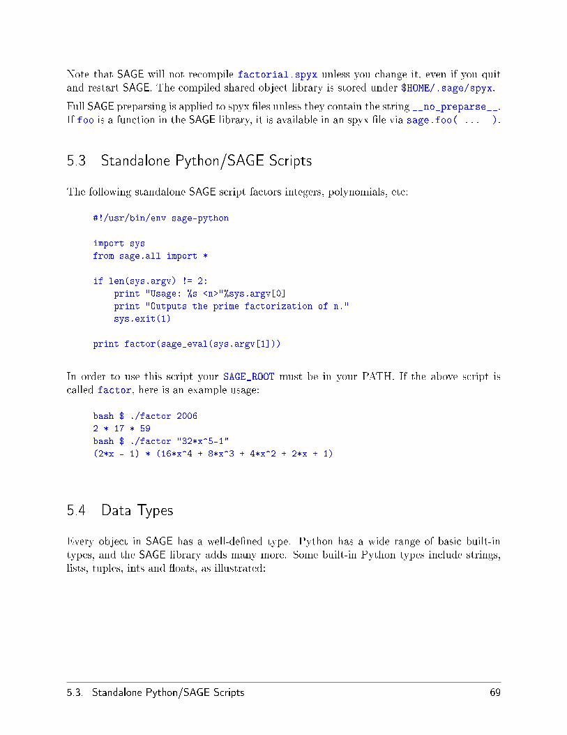
Note that SAGE will not recompile factorial.spyx unless you change it, even if you quitand restart SAGE. The compiled shared object library is stored under $HOME/.sage/spyx.
Full SAGE preparsing is applied to spyx �les unless they contain the string __no_preparse__.If foo is a function in the SAGE library, it is available in an spyx �le via sage.foo( ... ).
5.3 Standalone Python/SAGE Scripts
The following standalone SAGE script factors integers, polynomials, etc:
#!/usr/bin/env sage-python
import sys
from sage.all import *
if len(sys.argv) != 2:
print "Usage: %s <n>"%sys.argv[0]
print "Outputs the prime factorization of n."
sys.exit(1)
print factor(sage_eval(sys.argv[1]))
In order to use this script your SAGE_ROOT must be in your PATH. If the above script iscalled factor, here is an example usage:
bash $ ./factor 2006
2 * 17 * 59
bash $ ./factor "32*x^5-1"
(2*x - 1) * (16*x^4 + 8*x^3 + 4*x^2 + 2*x + 1)
5.4 Data Types
Every object in SAGE has a well-de�ned type. Python has a wide range of basic built-intypes, and the SAGE library adds many more. Some built-in Python types include strings,lists, tuples, ints and �oats, as illustrated:
5.3. Standalone Python/SAGE Scripts 69
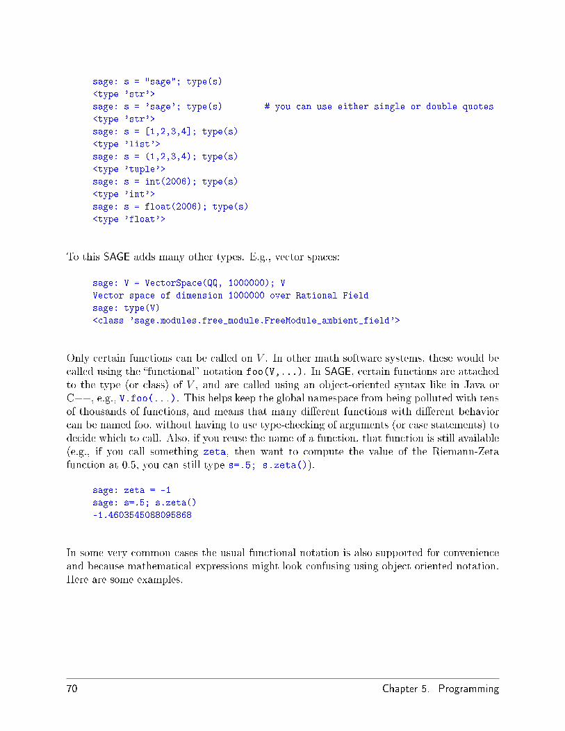
sage: s = "sage"; type(s)
<type 'str'>
sage: s = 'sage'; type(s) # you can use either single or double quotes
<type 'str'>
sage: s = [1,2,3,4]; type(s)
<type 'list'>
sage: s = (1,2,3,4); type(s)
<type 'tuple'>
sage: s = int(2006); type(s)
<type 'int'>
sage: s = float(2006); type(s)
<type 'float'>
To this SAGE adds many other types. E.g., vector spaces:
sage: V = VectorSpace(QQ, 1000000); V
Vector space of dimension 1000000 over Rational Field
sage: type(V)
<class 'sage.modules.free_module.FreeModule_ambient_field'>
Only certain functions can be called on V . In other math software systems, these would becalled using the �functional� notation foo(V,...). In SAGE, certain functions are attachedto the type (or class) of V , and are called using an object-oriented syntax like in Java orC++, e.g., V.foo(...). This helps keep the global namespace from being polluted with tensof thousands of functions, and means that many di�erent functions with di�erent behaviorcan be named foo, without having to use type-checking of arguments (or case statements) todecide which to call. Also, if you reuse the name of a function, that function is still available(e.g., if you call something zeta, then want to compute the value of the Riemann-Zetafunction at 0.5, you can still type s=.5; s.zeta()).
sage: zeta = -1
sage: s=.5; s.zeta()
-1.4603545088095868
In some very common cases the usual functional notation is also supported for convenienceand because mathematical expressions might look confusing using object-oriented notation.Here are some examples.
70 Chapter 5. Programming

sage: n = 2; n.sqrt()
1.4142135623730951
sage: sqrt(2)
1.4142135623730951
sage: V = VectorSpace(QQ,2)
sage: V.basis()
[
(1, 0),
(0, 1)
]
sage: basis(V)
[
(1, 0),
(0, 1)
]
sage: M = MatrixSpace(GF(7), 2); M
Full MatrixSpace of 2 by 2 dense matrices over Finite Field of size 7
sage: A = M([1,2,3,4]); A
[1 2]
[3 4]
sage: A.charpoly()
x^2 + 2*x + 5
sage: charpoly(A)
x^2 + 2*x + 5
To list all member functions for A, use tab completion. Just type A., then type the [tab]
key on your keyboard, as explained in Section 3.6.
5.5 Lists, Tuples, and Sequence
The list data type stores elements of arbitrary type. Like in C, C++, etc. (but unlike moststandard computer algebra systems), the elements of the list are indexed starting from 0:
sage: v = [2, 3, 5, 'x', SymmetricGroup(3)]; v
[2, 3, 5, 'x', Symmetric group of order 3! as a permutation group]
sage: type(v)
<type 'list'>
sage: v[0]
2
sage: v[2]
5
5.5. Lists, Tuples, and Sequence 71

Note: When indexing into a list, the index must be a Python int! A SAGE Integer will notwork. The preparser doesn't change integer literals to Python ints when they are indexinglists. However, if you index a list with a variable, you must be careful.
sage: v = [1,2,3]
sage: v[2]
3
sage: n = 2 # SAGE Integer
sage: v[n] # bad
Traceback (most recent call last):
...
TypeError: list indices must be integers
sage: v[int(n)] # good
3
(This is annoying, but it is good from a performance point of view.)
The range function creates a list of Python int's (not SAGE Integers):
sage: range(1, 15)
[1, 2, 3, 4, 5, 6, 7, 8, 9, 10, 11, 12, 13, 14]
This is useful when using list comprehensions to construct lists:
sage: L = [factor(n) for n in range(1, 15)]
sage: print L
[1, 2, 3, 2^2, 5, 2 * 3, 7, 2^3, 3^2, 2 * 5, 11, 2^2 * 3, 13, 2 * 7]
sage: L[12]
13
sage: type(L[12])
<class 'sage.structure.factorization.Factorization'>
sage: [factor(n) for n in range(1, 15) if is_odd(n)]
[1, 3, 5, 7, 3^2, 11, 13]
For more about how to create lists using list comprehensions, see [PyT].
List slicing is a wonderful feature. If L is a list, then L[m:n] returns the sublist of L obtainedby starting at the mth element and stopping at the (n− 1)st element, as illustrated below.
72 Chapter 5. Programming

sage: L = [factor(n) for n in range(1, 20)]
sage: L[4:9]
[5, 2 * 3, 7, 2^3, 3^2]
sage: print L[:4]
[1, 2, 3, 2^2]
sage: L[14:4]
[]
sage: L[14:]
[3 * 5, 2^4, 17, 2 * 3^2, 19]
Tuples are similar to lists, except they are immutable, meaning once they are created theycan't be changed.
sage: v = (1,2,3,4); v
(1, 2, 3, 4)
sage: type(v)
<type 'tuple'>
sage: v[1] = 5
Traceback (most recent call last):
...
TypeError: object does not support item assignment
Sequences are a third list-oriented SAGE type. Unlike lists and tuples, Sequence is not built�in Python type. By default, a sequence is mutable, but using the Sequence class methodset_immutable, it can be set to be immutable, as the following example illustrates. Allelements of a sequence have a common parent, called the sequences universe.
sage: v = Sequence([1,2,3,4/5])
sage: v
[1, 2, 3, 4/5]
sage: type(v)
<class 'sage.structure.sequence.Sequence'>
sage: type(v[1])
<type 'rational.Rational'>
sage: v.universe()
Rational Field
sage: v.is_immutable()
False
sage: v.set_immutable()
sage: v[0] = 3
Traceback (most recent call last):
...
ValueError: object is immutable; please change a copy instead.
5.5. Lists, Tuples, and Sequence 73
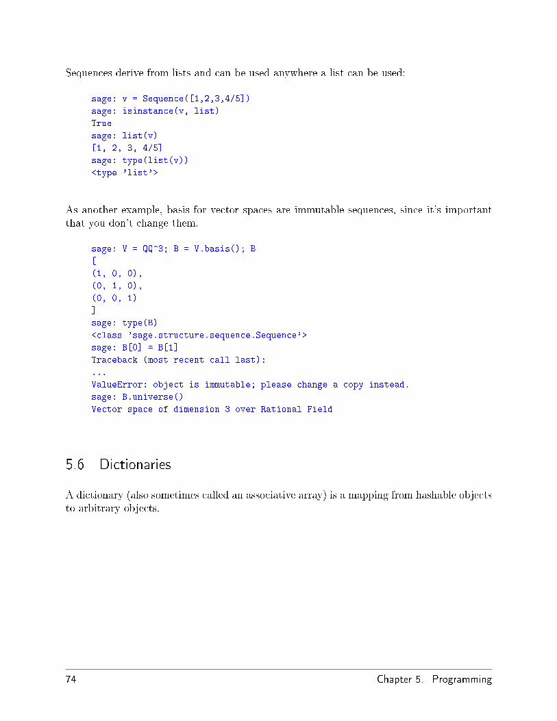
Sequences derive from lists and can be used anywhere a list can be used:
sage: v = Sequence([1,2,3,4/5])
sage: isinstance(v, list)
True
sage: list(v)
[1, 2, 3, 4/5]
sage: type(list(v))
<type 'list'>
As another example, basis for vector spaces are immutable sequences, since it's importantthat you don't change them.
sage: V = QQ^3; B = V.basis(); B
[
(1, 0, 0),
(0, 1, 0),
(0, 0, 1)
]
sage: type(B)
<class 'sage.structure.sequence.Sequence'>
sage: B[0] = B[1]
Traceback (most recent call last):
...
ValueError: object is immutable; please change a copy instead.
sage: B.universe()
Vector space of dimension 3 over Rational Field
5.6 Dictionaries
A dictionary (also sometimes called an associative array) is a mapping from hashable objectsto arbitrary objects.
74 Chapter 5. Programming

sage: d = {1:5, 'sage':17, ZZ:GF(7)}
sage: type(d)
<type 'dict'>
sage: d.keys()
[Integer Ring, 1, 'sage']
sage: d['sage']
17
sage: d[ZZ]
Finite Field of size 7
sage: d[1]
5
The third key illustrates that the indexes of a dictionary can be complicated, e.g., the ringof integers.
You can turn the above dictionary into a list with the same data:
sage: d.items()
[(Integer Ring, Finite Field of size 7), (1, 5), ('sage', 17)]
A common idiom is to iterate through the pairs of in a dictionary:
sage: d = {2:4, 3:9, 4:16}
sage: [a*b for a, b in d.iteritems()]
[8, 27, 64]
A dictionary is unordered, as the last output illustrates.
5.7 Sets
Python has a built-in set type. The main feature it o�ers is very fast lookup of whether anelement is in the set or not, along with standard set-theoretic operations.
5.7. Sets 75

sage: X = set([1,19,'a']); Y = set([1,1,1, 2/3])
sage: X
set(['a', 1, 19])
sage: Y
set([1, 2/3])
sage: 'a' in X
True
sage: 'a' in Y
False
sage: X.intersection(Y)
set([1])
SAGE also has its own set type that is (in some cases) implemented using the built-in Pythonset type, but has a little bit of extra SAGE-related functionality. Create a SAGE set usingSet(...). For example,
sage: X = Set([1,19,'a']); Y = Set([1,1,1, 2/3])
sage: X
{'a', 1, 19}
sage: Y
{1, 2/3}
sage: X.intersection(Y)
{1}
sage: print latex(Y)
\left\{1, \frac{2}{3}\right\}
sage: Set(ZZ)
Set of elements of Integer Ring
5.8 Iterators
Iterators are a recent addition to Python that are particulary useful in mathematics appli-cations. Here are several examples; see [PyT] for more details. We make an iterator overthe squares of the nonnegative integers up to 10000000.
76 Chapter 5. Programming
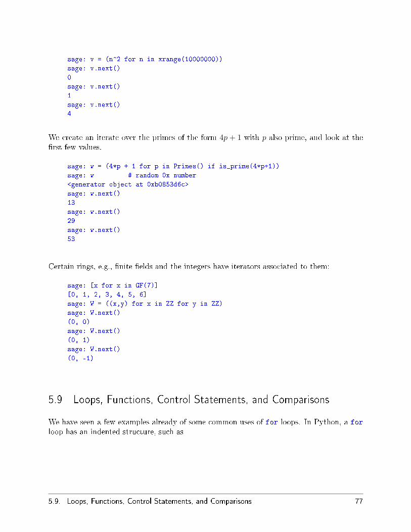
sage: v = (n^2 for n in xrange(10000000))
sage: v.next()
0
sage: v.next()
1
sage: v.next()
4
We create an iterate over the primes of the form 4p + 1 with p also prime, and look at the�rst few values.
sage: w = (4*p + 1 for p in Primes() if is_prime(4*p+1))
sage: w # random 0x number
<generator object at 0xb0853d6c>
sage: w.next()
13
sage: w.next()
29
sage: w.next()
53
Certain rings, e.g., �nite �elds and the integers have iterators associated to them:
sage: [x for x in GF(7)]
[0, 1, 2, 3, 4, 5, 6]
sage: W = ((x,y) for x in ZZ for y in ZZ)
sage: W.next()
(0, 0)
sage: W.next()
(0, 1)
sage: W.next()
(0, -1)
5.9 Loops, Functions, Control Statements, and Comparisons
We have seen a few examples already of some common uses of for loops. In Python, a for
loop has an indented structure, such as
5.9. Loops, Functions, Control Statements, and Comparisons 77

>>> for i in range(5):
print(i)
0
1
2
3
4
Note the colon at the end of the for statement (there is no �do� or �od� as in GAP or Maple),and the indentation before the �body� of the loop, namely print(i). This indentation isimportant. In SAGE, the indentation is automatically put in for you when you hit enterafter a �:�, as illustrated below.
sage: for i in range(5):
print(i) # now hit enter twice
0
1
2
3
4
sage:
The symbol = is used for assignment. The symbol == is used to check for equality:
sage: for i in range(15):
if gcd(i,15) == 1:
print(i)
1
2
4
7
8
11
13
14
Keep in mind how indentation determines the block structure for if, for, and while state-ments:
78 Chapter 5. Programming
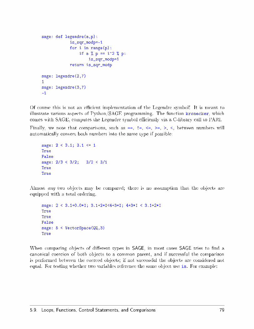
sage: def legendre(a,p):
is_sqr_modp=-1
for i in range(p):
if a % p == i^2 % p:
is_sqr_modp=1
return is_sqr_modp
sage: legendre(2,7)
1
sage: legendre(3,7)
-1
Of course this is not an e�cient implementation of the Legendre symbol! It is meant toillustrate various aspects of Python/SAGE programming. The function kronecker, whichcomes with SAGE, computes the Legendre symbol e�ciently via a C-library call to PARI.
Finally, we note that comparisons, such as ==, !=, <=, >=, >, <, between numbers willautomatically convert both numbers into the same type if possible:
sage: 2 < 3.1; 3.1 <= 1
True
False
sage: 2/3 < 3/2; 3/2 < 3/1
True
True
Almost any two objects may be compared; there is no assumption that the objects areequipped with a total ordering.
sage: 2 < 3.1+0.0*I; 3.1+2*I<4+3*I; 4+3*I < 3.1+2*I
True
True
False
sage: 5 < VectorSpace(QQ,3)
True
When comparing objects of di�erent types in SAGE, in most cases SAGE tries to �nd acanonical coercion of both objects to a common parent, and if successful the comparisonis performed between the coerced objects; if not successful the objects are considered notequal. For testing whether two variables reference the same object use is. For example:
5.9. Loops, Functions, Control Statements, and Comparisons 79

sage: 1 is 2/2
False
sage: 1 is 1
False
sage: 1 == 2/2
True
In the following two lines the �rst equality is False because there is no canonical morphismQ → F5, hence no canonical way to compare the 1 in F5 to the 1 ∈ Q. In contrast, thereis a canonical map Z → F5, hence the second comparison is True. Note also that the orderdoesn't matter.
sage: GF(5)(1) == QQ(1); QQ(1) == GF(5)(1)
False
False
sage: GF(5)(1) == ZZ(1); ZZ(1) == GF(5)(1)
True
True
sage: ZZ(1) == QQ(1)
True
WARNING: Comparison in SAGE is more restrictive than in Magma, which declares the1 ∈ F5 equal to 1 ∈ Q.
sage: magma('GF(5)!1 eq Rationals()!1') # optional magma required
true
5.10 Adding Your Own Methods to a SAGE Class
Section Author: Martin Albrecht ([email protected])
If you want to extend SAGE by adding your own methods to a SAGE class there is a convenientway built into Python. You should understand the basics of object-oriented programmingin Python in order to understand how to override class methods (see, e.g., the excellent freePython tutorial [PyT]). In Python nearly everything is changeable, so for instance you canalter class functions on the �y. We will use this by adding a rather silly method to theMatrix class in the following example. We start by writing a MatrixMixIn class:
80 Chapter 5. Programming

class MatrixMixIn:
def ncols_plus_nrows(self):
"""
Return the number of rows plus the number of columns.
"""
return self.ncols() + self.nrows()
Now we load the �le where we de�ned this class into SAGE and add this class as a superclassto the Matrix class (you could also just paste the above code into your SAGE session).The superclasses are stored in an attribute called __bases__ for every class (except builtincompiled extension classes). It is a tuple of classes, so we just add our class to this tuple:
sage: sage.matrix.matrix.Matrix.__bases__ += (MatrixMixIn,)
You can also get the class of an object using the __class__ attribute of any object of thatclass:
sage: A = Matrix(Integers(8),2,2,[1,2,3,4])
sage: A.__class__
<class 'sage.matrix.matrix.Matrix_generic_dense'>
But note that we cannot write Matrix.__bases__ above as Matrix is a function to constructmatrices and not the Matrix class. This is not always the case, but it's just the way Matricesare treated in SAGE:
sage: type(Matrix)
<type 'function'>
sage: type(sage.matrix.matrix.Matrix)
<type 'type'>
sage: type(Integer)
<type 'type'>
Now every instance of this class and every instance of any class inheriting from this classhas our new method.
5.10. Adding Your Own Methods to a SAGE Class 81
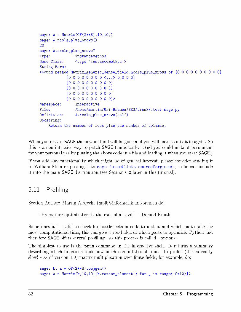
sage: A = Matrix(GF(2**8),10,10,)
sage: A.ncols_plus_nrows()
20
sage: A.ncols_plus_nrows?
Type: instancemethod
Base Class: <type 'instancemethod'>
String Form:
<bound method Matrix_generic_dense_field.ncols_plus_nrows of [0 0 0 0 0 0 0 0 0 0]
[0 0 0 0 0 0 0 0 <...> 0 0 0 0]
[0 0 0 0 0 0 0 0 0 0]
[0 0 0 0 0 0 0 0 0 0]
[0 0 0 0 0 0 0 0 0 0]
[0 0 0 0 0 0 0 0 0 0]>
Namespace: Interactive
File: /home/martin/Uni-Bremen/BES/trunk/.test.sage.py
Definition: A.ncols_plus_nrows(self)
Docstring:
Return the number of rows plus the number of columns.
When you restart SAGE the new method will be gone and you will have to mix it in again. Sothis is a non intrusive way to patch SAGE temporarily. (And you could make it permanentfor your personal use by putting the above code in a �le and loading it when you start SAGE.)
If you add any functionality which might be of general interest, please consider sending itto William Stein or posting it to [email protected], so he can includeit into the main SAGE distribution (see Section 6.2 later in this tutorial).
5.11 Pro�ling
Section Author: Martin Albrecht ([email protected])
�Premature optimization is the root of all evil.� � Donald Knuth
Sometimes it is useful to check for bottlenecks in code to understand which parts take themost computational time; this can give a good idea of which parts to optimize. Python andtherefore SAGE o�ers several pro�ling�as this process is called�options.
The simplest to use is the prun command in the interactive shell. It returns a summarydescribing which functions took how much computational time. To pro�le (the currentlyslow! - as of version 1.0) matrix multiplication over �nite �elds, for example, do:
sage: k, a = GF(2**8).objgen()
sage: A = Matrix(k,10,10,[k.random_element() for _ in range(10*10)])
82 Chapter 5. Programming

sage: prun B = A*A
32893 function calls in 1.100 CPU seconds
Ordered by: internal time
ncalls tottime percall cumtime percall filename:lineno(function)
12127 0.160 0.000 0.160 0.000 :0(isinstance)
2000 0.150 0.000 0.280 0.000 matrix.py:2235(__getitem__)
1000 0.120 0.000 0.370 0.000 finite_field_element.py:392(__mul__)
1903 0.120 0.000 0.200 0.000 finite_field_element.py:47(__init__)
1900 0.090 0.000 0.220 0.000 finite_field_element.py:376(__compat)
900 0.080 0.000 0.260 0.000 finite_field_element.py:380(__add__)
1 0.070 0.070 1.100 1.100 matrix.py:864(__mul__)
2105 0.070 0.000 0.070 0.000 matrix.py:282(ncols)
...
Here ncalls is the number of calls, tottime is the total time spent in the given function(and excluding time made in calls to sub-functions), percall is the quotient of tottimedivided by ncalls. cumtime is the total time spent in this and all sub-functions (i.e., frominvocation until exit), percall is the quotient of cumtime divided by primitive calls, andfilename:lineno(function) provides the respective data of each function. The rule ofthumb here is: The higher the function in that listing the more expensive it is. Thus it ismore interesting for optimization.
As usual, prun? provides details on how to use the pro�ler and understand the output.
The pro�ling data may be written to an object as well to allow closer examination:
sage: prun -r A*A
sage: stats = _
sage: ?stats
Please note that you cannot do a stats = prun -r A*A for some internal reason.
For a nice graphical representation of pro�ling data you can use the hotshot pro�ler, a smallscript called hotshot2cachetree and the program kcachegrind (Unix only). The sameexample with the hotshot pro�ler:
sage: k, a = GF(2**8).objgen()
sage: A = Matrix(k,10,10,[k.random_element() for _ in range(10*10)])
sage: import hotshot
sage: filename = "pythongrind.prof"
sage: prof = hotshot.Profile(filename, lineevents=1)
5.11. Pro�ling 83
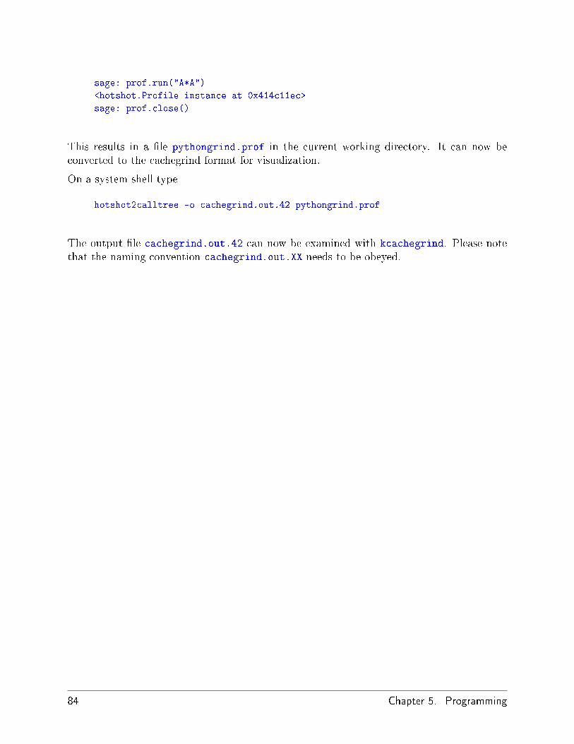
sage: prof.run("A*A")
<hotshot.Profile instance at 0x414c11ec>
sage: prof.close()
This results in a �le pythongrind.prof in the current working directory. It can now beconverted to the cachegrind format for visualization.
On a system shell type
hotshot2calltree -o cachegrind.out.42 pythongrind.prof
The output �le cachegrind.out.42 can now be examined with kcachegrind. Please notethat the naming convention cachegrind.out.XX needs to be obeyed.
84 Chapter 5. Programming

CHAPTER
SIX
Afterword
6.1 Why Python?
6.1.1 Advantages to Python
The primary implementation language of SAGE is Python (see [Py]), though code that mustbe fast is implemented in a compiled language. Using Python has several advantages:
� Object saving is well-supported in Python. There is extensive support in Python forsaving (nearly) arbitrary objects to disk �les or a database.
� Excellent support for documentation of functions and packages in the source code,including automatic extraction of documentation and automatic testing of all examples.The examples are automatically tested regularly and guaranteed to work as indicated.
� Memory management: Python now has a well thought out and robust memorymanager and garbage collector that correctly deals with circular references, and allowsfor local variables in �les.
� Python has many packages available now that might be of great interest to users ofSAGE: numerical analysis and linear algebra, 2D and 3D visualization, networking (fordistributed computations and servers, e.g., via twisted), database support, etc.
� Portability: Python is easy to compile from source on most platforms in minutes.
� Exception handling: Python has a sophisticated and well thought out system ofexception handling, whereby programs gracefully recover even if errors occur in codethey call.
� Debugger: Python includes a debugger, so when code fails for some reason, the userreceives an error message, extensive stack trace, and can inspect the state of all relevantvariables and move up and down the stack.
� Pro�ler: There is a Python pro�ler, which runs code and creates a report detailinghow many times and for how long each function was called.
85
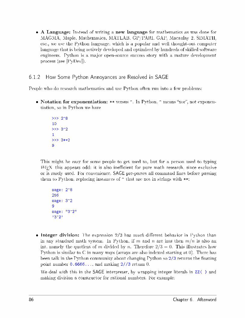
� A Language: Instead of writing a new language for mathematics as was done forMAGMA, Maple, Mathematica, MATLAB, GP/PARI, GAP, Macaulay 2, SIMATH,etc., we use the Python language, which is a popular and well thought-out computerlanguage that is being actively developed and optimized by hundreds of skilled softwareengineers. Python is a major open-source success story with a mature developmentprocess (see [PyDev]).
6.1.2 How Some Python Annoyances are Resolved in SAGE
People who do research mathematics and use Python often run into a few problems:
� Notation for exponentiation: ** versus ^. In Python, ^ means �xor�, not exponen-tiation, so in Python we have
>>> 2^8
10
>>> 3^2
1
>>> 3**2
9
This might be easy for some people to get used to, but for a person used to typingLATEX this appears odd; it is also ine�cient for pure math research, since exclusiveor is rarely used. For convenience, SAGE pre-parses all command lines before passingthem to Python, replacing instances of ^ that are not in strings with **:
sage: 2^8
256
sage: 3^2
9
sage: "3^2"
'3^2'
� Integer division: The expression 2/3 has much di�erent behavior in Python thanin any standard math system. In Python, if m and n are ints then m/n is also anint, namely the quotient of m divided by n. Therefore 2/3 = 0. This illustrates howPython is similar to C in many ways (arrays are also indexed starting at 0). There hasbeen talk in the Python community about changing Python so 2/3 returns the �oatingpoint number 0.6666..., and making 2//3 return 0.
We deal with this in the SAGE interpreter, by wrapping integer literals in ZZ( ) andmaking division a constructor for rational numbers. For example:
86 Chapter 6. Afterword

sage: 2/3
2/3
sage: 2//3
0
sage: int(2)/int(3)
0
� Long integers: Python has native support for arbitrary precision integers, in additionto C-int's. These are signi�cantly slower than what GMP provides, and have theextremely annoying property that they print with an L at the end to distinguish themfrom int's (and this won't change any time soon). SAGE also implements arbitraryprecision integers, using the GMP C-library, and these print without an L.
Rather than modifying the Python interpreter (as I've heard some people have done forinternal projects), we use the Python language exactly as is, and write a pre-parser forIPython so that the command line behavior of IPython is what a mathematician expects.This means any existing Python code can be used in SAGE. However, one must still obeythe standard Python rules when writing packages that will be imported into SAGE.
Note: To install a random Python library that you �nd on the internet, follow the direc-tions, but run sage-python instead of python. Very often this means typing sage-python
setup.py install.
6.2 I would like to contribute somehow. How can I?
If you would like to contribute to SAGE, your help will be greatly appreciated! It can rangefrom substantial code contributions to simply adding to the SAGE documentation. Just emailWilliam Stein at [email protected] or post it to [email protected] look at the SAGE web site, where there is a long list of SAGE-related projects orderedby priority and category.
SAGE is now su�ciently mature that there are tons of projects to work on that involveexposing more functionality of the included backend systems (Gap, PARI, Singular, etc.).This is mostly fun design work, since the really hard nitty gritty algorithmic implementationdetails and optimization has already been done, e.g., in Gap or PARI or Singular.
If you submit or post your code, put a copyright notice on the code that makes clear thatyou are releasing it under the GPL or a more liberal license. I cannot include any code withSAGE that doesn't have an explicitly stated GPL-compatible copyright.
For example, you could put the following at the top of your source �le.
6.2. I would like to contribute somehow. How can I? 87

##############################################################################
# SAGE: System for Algebra and Geometry Experimentation
#
# Copyright (C) 2006 Your name <your email>
# Copyright (C) 2006 William Stein <[email protected]> (optional)
#
# Distributed under the terms of the GNU General Public License (GPL)
#
# http://www.gnu.org/licenses/
##############################################################################
Note: It is not required for you to share the copyright with me, though I prefer it since itgives me �exibility regarding the code.
6.3 How do I reference SAGE?
If you write a paper using SAGE, please reference computations done with SAGE by including[SJ] in your bibliography. Moreover, please attempt to track down what components of SAGEare used for your computation, e.g., PARI?, Gap?, Singular? Maxima? and also cite thosesystems. If you are in doubt about what software your computation uses, feel free to contactme ([email protected]) and I'll try to �gure it out. See Section 2.2.1 for further discussionof this point.
* * *
If you happen to have just read straight through this tutorial, and have some sense of howlong it took you, please let me know (email [email protected]).
Have fun with SAGE!
88 Chapter 6. Afterword
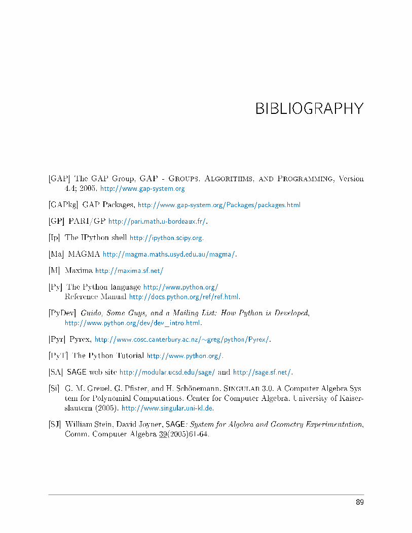
BIBLIOGRAPHY
[GAP] The GAP Group, GAP - Groups, Algorithms, and Programming, Version4.4; 2005, http://www.gap-system.org
[GAPkg] GAP Packages, http://www.gap-system.org/Packages/packages.html
[GP] PARI/GP http://pari.math.u-bordeaux.fr/.
[Ip] The IPython shell http://ipython.scipy.org.
[Ma] MAGMA http://magma.maths.usyd.edu.au/magma/.
[M] Maxima http://maxima.sf.net/
[Py] The Python language http://www.python.org/
Reference Manual http://docs.python.org/ref/ref.html.
[PyDev] Guido, Some Guys, and a Mailing List: How Python is Developed,http://www.python.org/dev/dev_intro.html.
[Pyr] Pyrex, http://www.cosc.canterbury.ac.nz/∼greg/python/Pyrex/.
[PyT] The Python Tutorial http://www.python.org/.
[SA] SAGE web site http://modular.ucsd.edu/sage/ and http://sage.sf.net/.
[Si] G.-M. Greuel, G. P�ster, and H. Schönemann. Singular 3.0. A Computer Algebra Sys-tem for Polynomial Computations. Center for Computer Algebra, University of Kaiser-slautern (2005). http://www.singular.uni-kl.de.
[SJ] William Stein, David Joyner, SAGE: System for Algebra and Geometry Experimentation,Comm. Computer Algebra 39(2005)61-64.
89

90
INDEX
<=, 79=, 78==, 78>=, 79
adding methods, 80attach, 68attach into SAGE, 67
CC, 6Chinese remainder theorem, 16classes in SAGE, 80command line, using SAGE in, 41cPickle, 53Cremona database, 25, 28
data type in SAGE, 69def, example of, 78dictionary
creating a, 74Dirichlet characters, 17docstring for SAGE functions, 50documentation, viewing inline, 52
eigenvalues, 63eigenvectors, 63elliptic curves, 25
associated L-series, 27conductor, 26j-invariant, 27
error mesaages in SAGE, 47Euclidean algorithm, 15Euler phi-function, 15Euler's method for 1st order DEs, 35exitting, 41
for loops, 77
GAP, 61gcd, 14goals for SAGE, 2GP/PARI, 59groups
permutation, 23
help, 50history of SAGE commands, 42
I, 6if-then statements, 77immutable, 73installation, 1interactive shell, using SAGE in, 41
Laplace transform solution of DEs, 33Laurent series, 11list
creating a, 71slicing, 72
load into SAGE, 67logging your session, 43
macro, SAGE, 42matrix
creating a, 19echelon form, 20numerical computations with, 22row reduction, 20
Maxima, 63mixins, 80modular
form, 38symbols, 39
notation
91

functional, 70object oriented, 70
PARI, 59polynomial
ring of multivariate, 12polynomials
cyclotomic, 10ideal of, 14ring of univariate, 8SAGE, 8
prun, 82pyrex, 68Python and SAGE, 69, 85
QQ, 6quitting, 41
rational functions, 10readline commands, 49rings in SAGE, 5RR, 6
saveSAGE objects, 52SAGE session, 43, 55
sequencecreating a, 73
session, 41log, 43pasting into, 45SAGE, 41saving in konsole, 44
setcreating a, 75
Singular, 62spyx �les, 68
tab completion, 49time
with prun, 82time, cpu, 46time, wall, 46timing in SAGE, 45tuple
creating a, 73
unix escape, 43
ZZ, 6
92 Index


