Salinity Simulation with WRAP - TWRItwri.tamu.edu/reports/2009/tr317.pdf · Salinity Simulation ......

COLLEGE OF AGRICULTURE

AND LIFE SCIENCES

TR-317

2009

Salinity Simulation with WRAP

By Ralph A. Wurbs

Zachry Department of Civil Engineering Texas A&M University College Station, Texas

July 2009

Texas Water Resources Institute Technical Report No. 317 Texas A&M University System

College Station, Texas 77843-2118


TR-317 Texas Water Resources Institute College Station, Texas July 2009

by Ralph A. Wurbs Texas A&M University


by

Ralph A. Wurbs Texas A&M University

for the

Texas Commission on Environmental Quality Austin, Texas 78711-3087

Cosponsored with Supplemental Funding Support

from the

Fort Worth District, U.S. Army Corps of Engineers and

Texas Water Resources Institute, Texas A&M University System

Technical Report No. 317 Texas Water Resources Institute

The Texas A&M University System College Station, Texas 77843-2118

July 2009

TABLE OF CONTENTS Introduction................................................................................................................................. 1 Salinity Aspects of Water Availability Modeling ...................................................................... 1 Computer Programs, Data Files, and Input Records .................................................................. 2 Spatial Configuration .................................................................................................................. 4 Salinity Input Dataset.................................................................................................................. 7 Program SALIN .......................................................................................................................... 8 Volumes, Loads, and Concentrations ......................................................................................... 9 Salinity Simulation with Program SALT .................................................................................... 12 Reservoir Storage and Outflow Concentrations ........................................................................ 21 SALT Simulation Results ............................................................................................................ 34 TABLES Time Series, Summary, Frequency, and Reliability Tables ....................................... 39 Parameter Calibration Comparison Features ............................................................................. 40 Constant Salinity Simulation Example ...................................................................................... 41 Salinity Simulation Example ...................................................................................................... 43 References................................................................................................................................... 59 Appendix A Instructions for Preparing SALT Input Records ................................................. 61

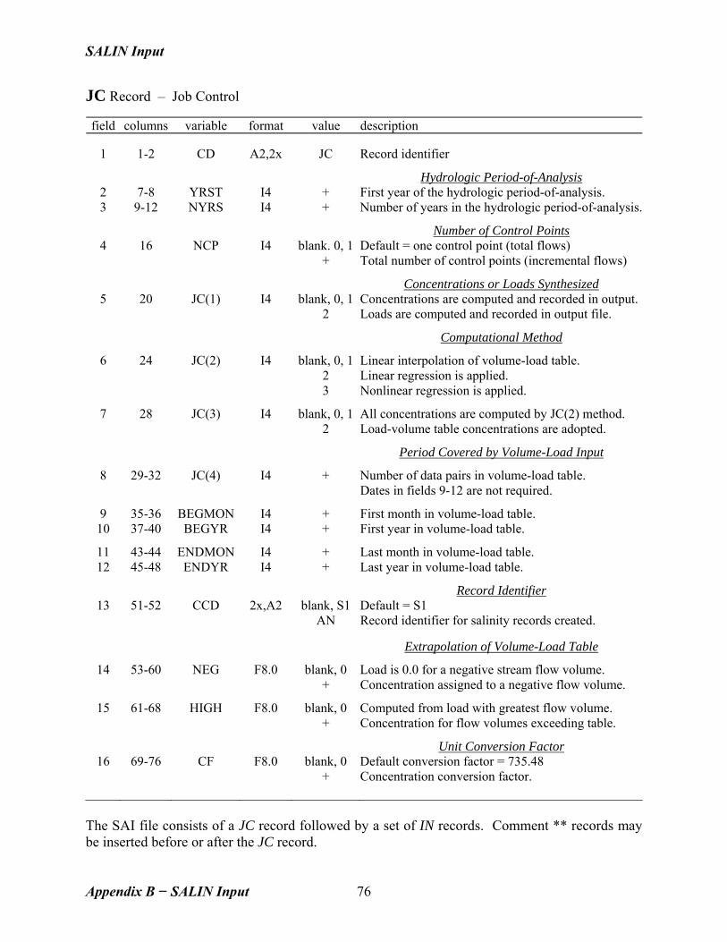
Appendix B Instructions for Preparing SALIN Input Records ............................................... 75

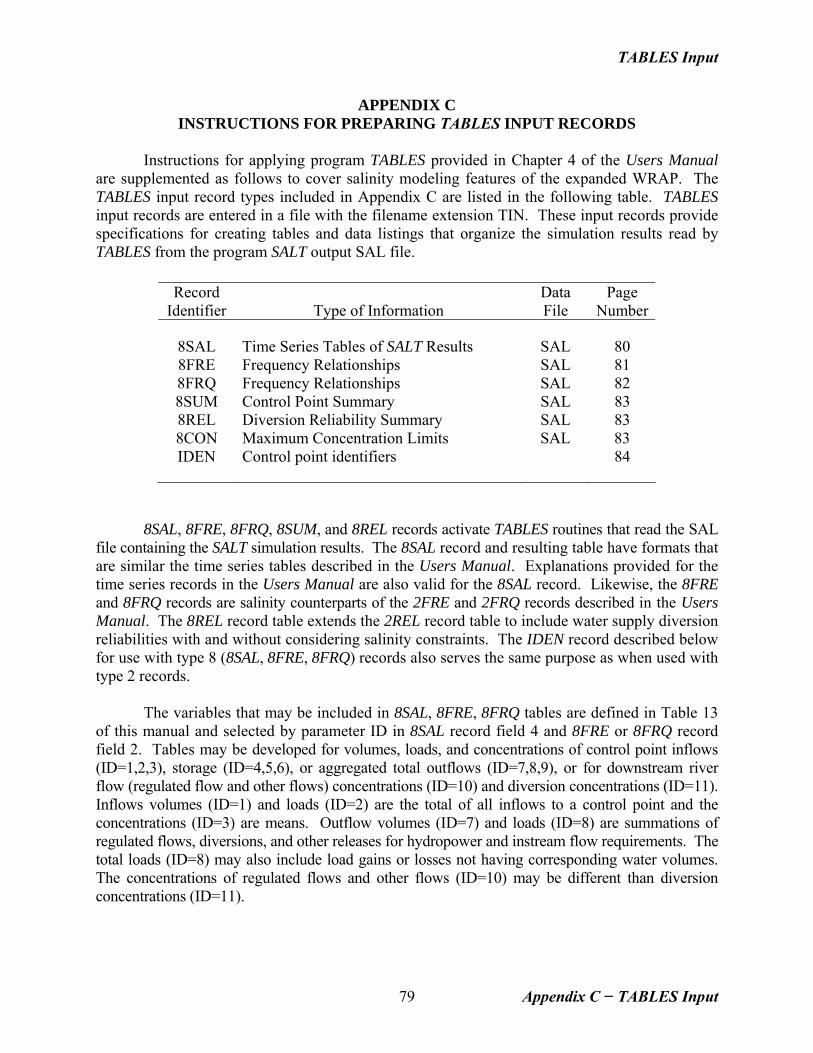
Appendix C Instructions for Preparing TABLES Input Records ............................................ 79

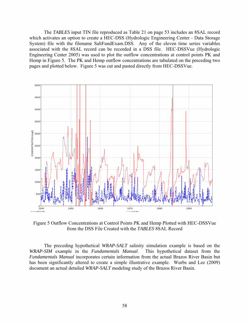
LIST OF FIGURES 1. Control Point Configuration ................................................................................................. 5 2. Organization of SALT Computations ................................................................................... 12 3 Outline of the Salinity Simulation Performed by Program SALT ....................................... 13 4 System Schematic for the Example ..................................................................................... 44 5. Outflow Concentrations at Control Points PK and Hemp Plotted with HEC-DSSVue from the DSS File Created with the TABLES 8SAL Record ................... 66

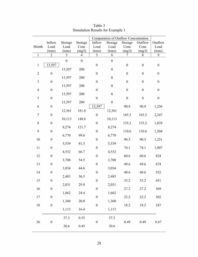
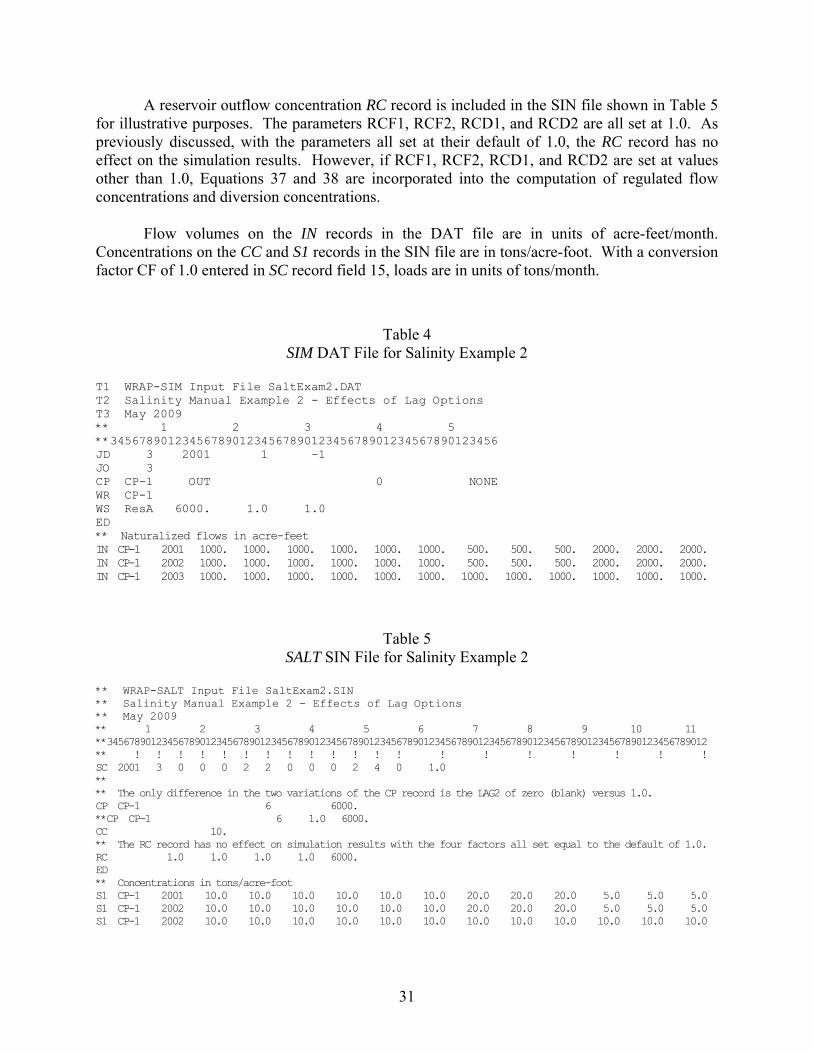
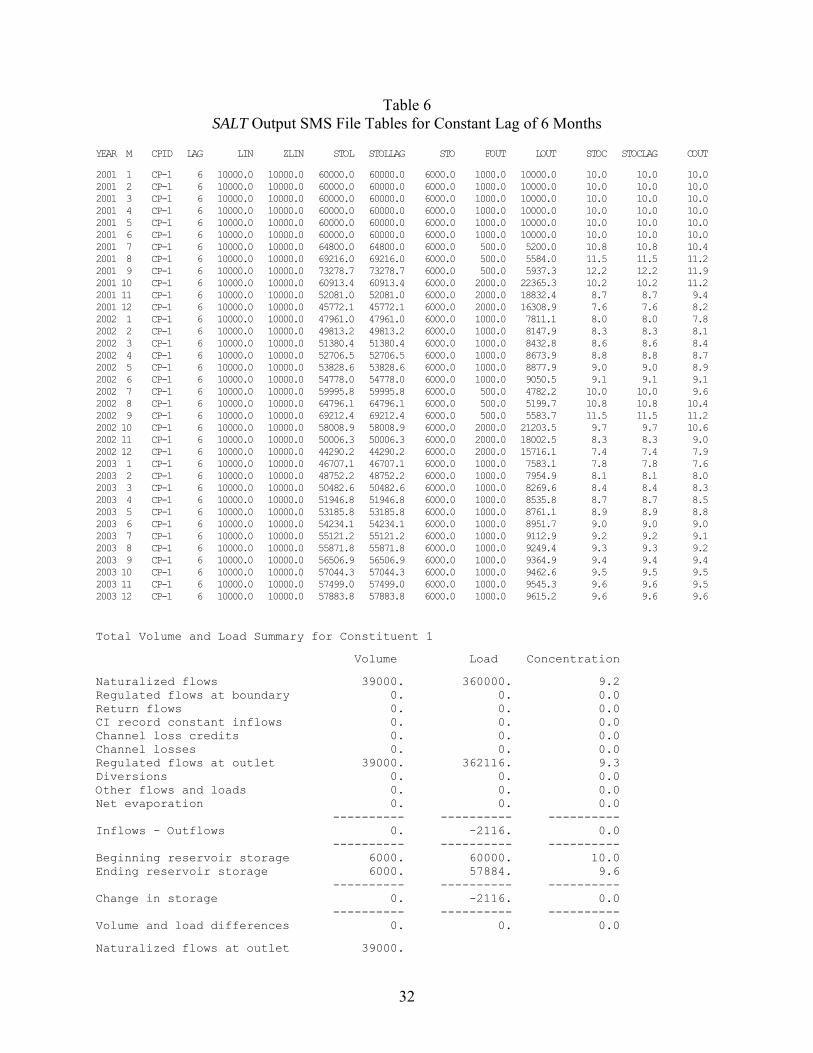
LIST OF TABLES 1. Components of Control Point Inflows and Outflows .......................................................... 11 2. Variables from SIM/SIMD Simulation Results ................................................................... 14 3. Simulation Results for Example 1 ........................................................................................ 28 4. SIM DAT File for Salinity Example 2 ................................................................................. 31 5. SALT SIN File for Salinity Example 2 ................................................................................ 31 6. SALT Output SMS File for Constant Lag of 6 Months ...................................................... 32

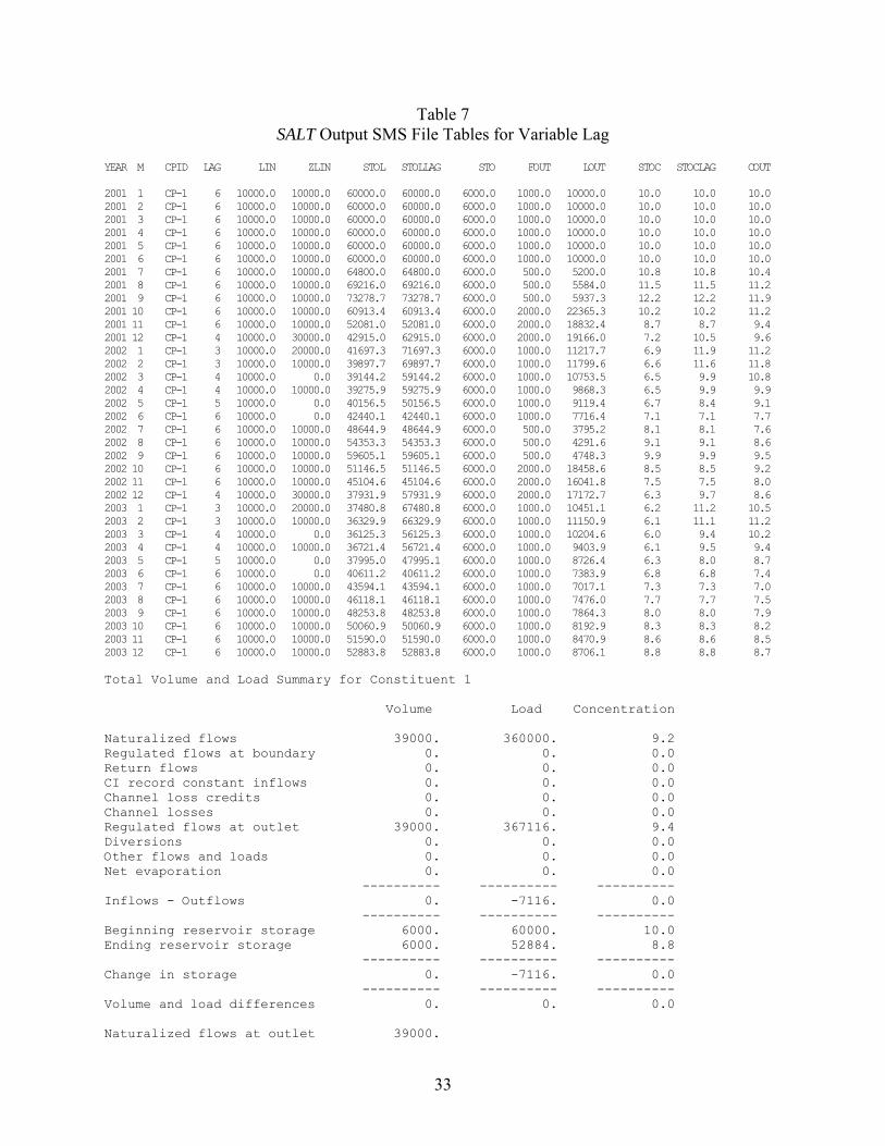
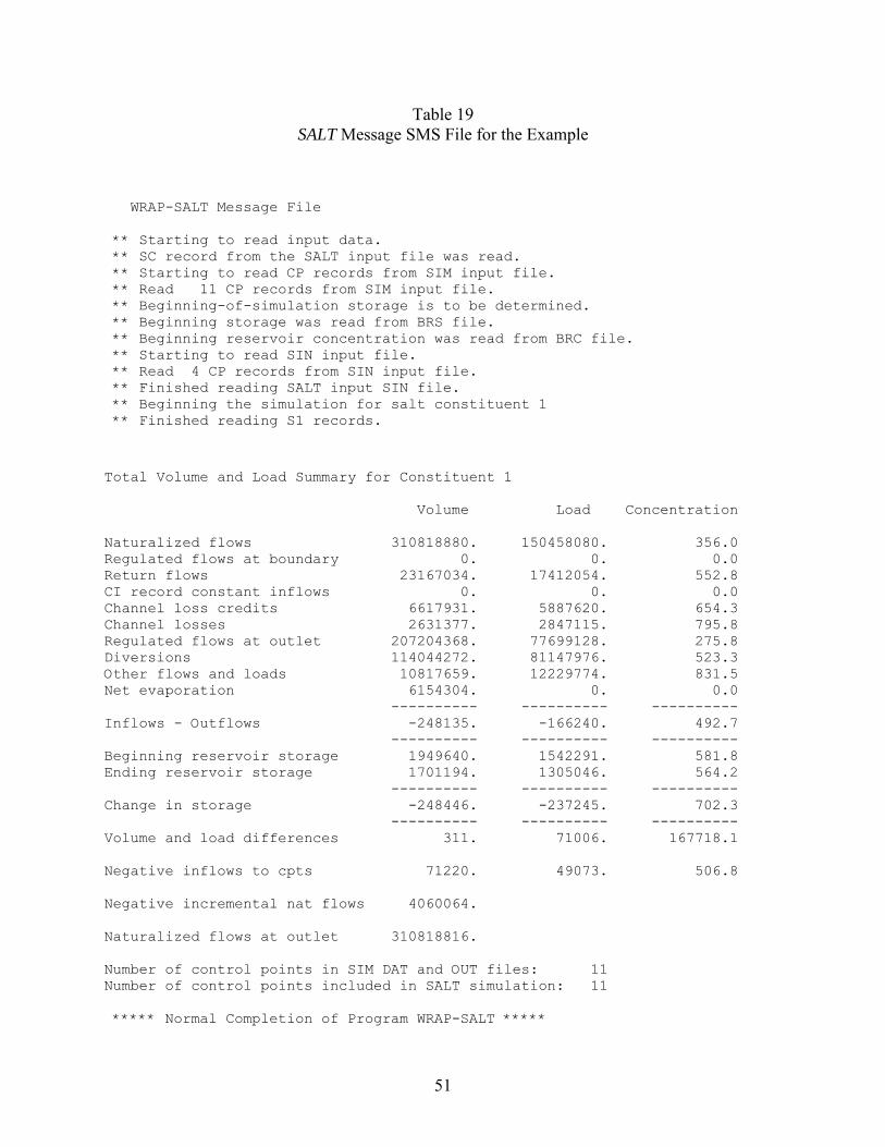
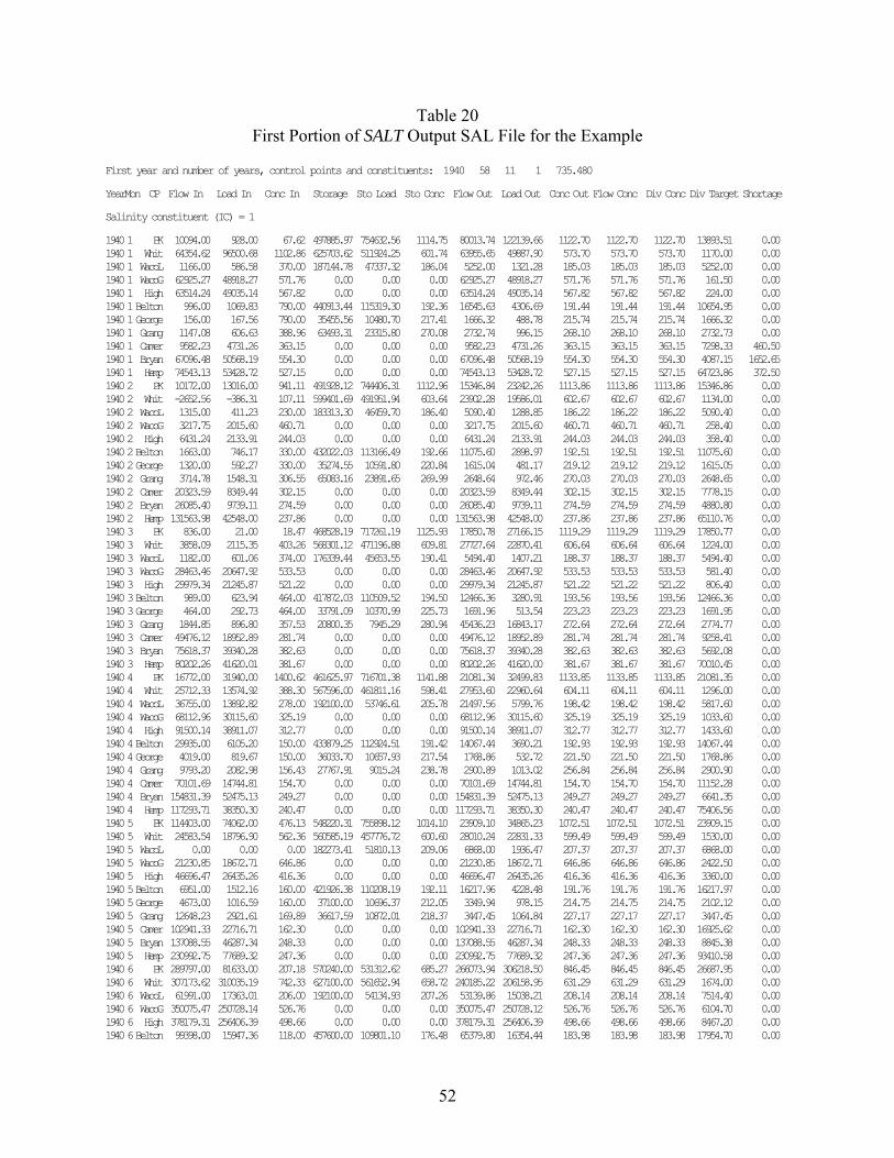
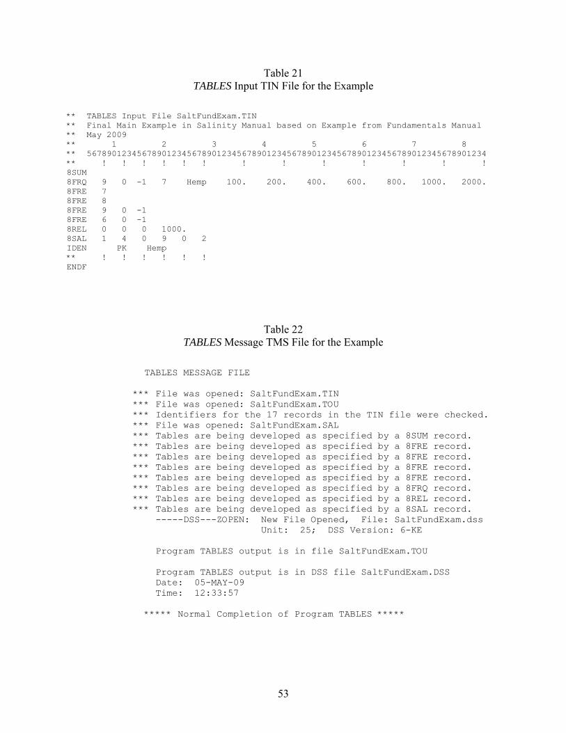
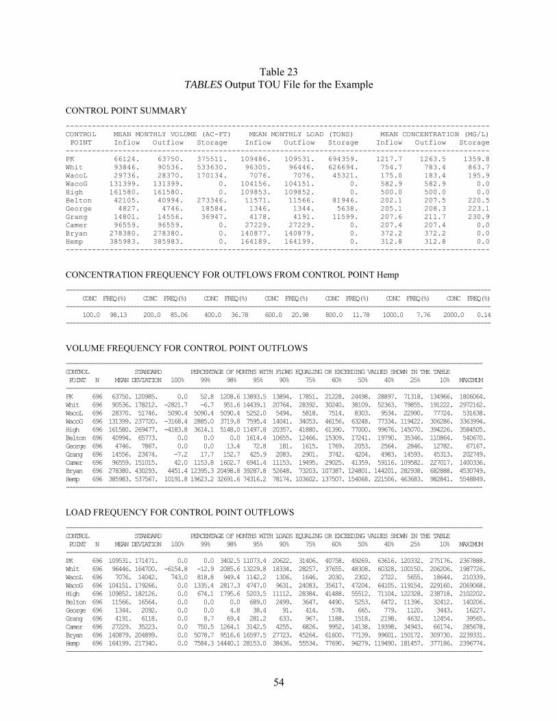
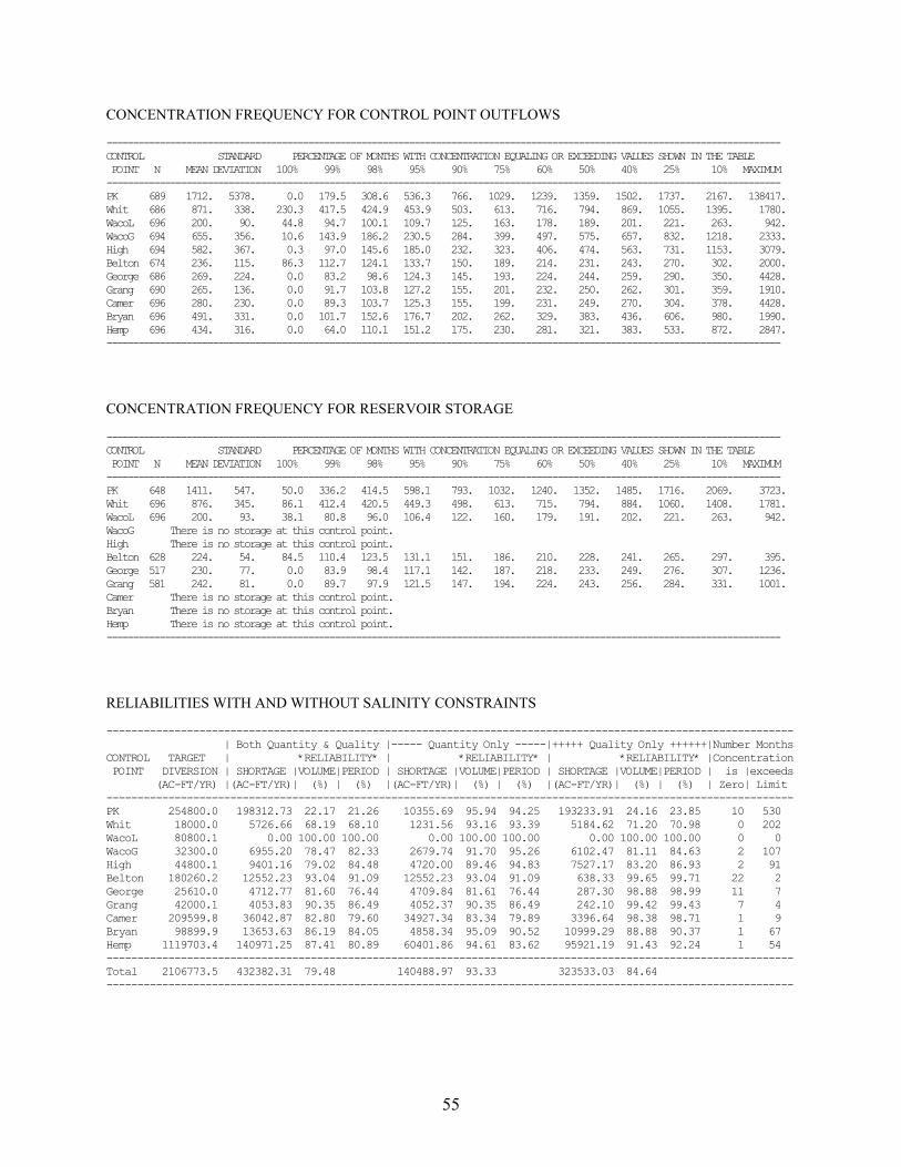
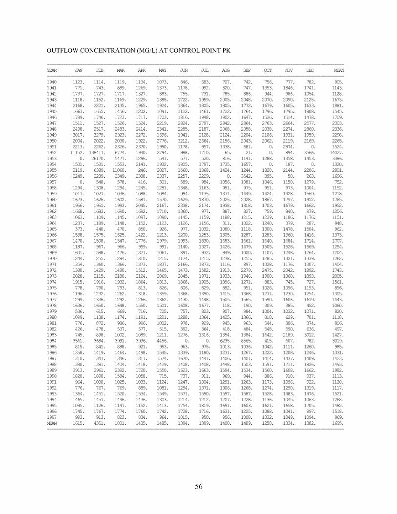
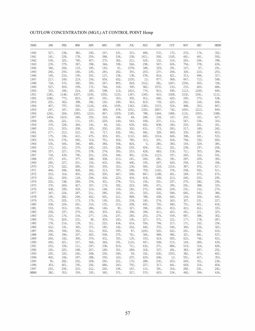
LIST OF TABLES (Continued) 7. SALT Output SMS File for Variable Lag ............................................................................ 33 8. Trace Messages Written to SMS File .................................................................................. 35 9. Variables in First Line of SMS Data Set ............................................................................. 35 10. Monthly Volume and Load Budget by Control Point SAL File Dataset ............................ 36 11. SMS File Table of Total Volume and Load for the Entire River/Reservoir System and Period-of-Analysis .............................................................. 37 12. Variables in SAL File ........................................................................................................... 39 13. Variables in 8SAL, 8FRE, and 8FRQ Record Tables ........................................................ 40 14. SALT SIN File for Salinity Example 3 ............................................................................... 42 15. Summary Table for Salinity Example 3 .............................................................................. 43 16. Beginning Reservoir Storage BRS File for the Example .................................................... 47 17. Reservoir Storage BRS File for the Example ...................................................................... 47 18. SALT Input SIN File for the Example .................................................................................. 48 19. SALT Message SMS File for the Example .......................................................................... 51 20. First Portion of SALT Output SAL File for the Example .................................................... 52 21. TABLES Input TIN File for the Example ............................................................................ 53 22. TABLES Message TMS File for the Example ..................................................................... 53 23. TABLES Output TOU File for the Example ......................................................................... 54

1

Introduction The Water Rights Analysis Package (WRAP) modeling system is documented by basic reference and users manuals and supplemental manuals covering specific features, including this manual which deals specifically with salinity simulation capabilities. This Salinity Manual is an extension of the Reference and Users Manuals (Wurbs 2009). Salinity tracking components of WRAP consist of the simulation model SALT, auxiliary program SALIN, and table building routines in the program TABLES. Program SALT combines water quantity data read from the SIM or SIMD simulation results file with concentrations or loads of inflows from a salinity input file. The program SALIN provides optional routines designed to assist in developing salinity input data for program SALT. Options in TABLES organize the SALT salinity simulation results and develop frequency statistics. The combined SIM, SALT, and TABLES model is designed for simulating water quality throughout a system of river reaches and reservoirs for alternative scenarios of water use, reservoir system operating policies, and salt control measures. Loads and concentrations of water quality constituents in stream flows, reservoir storage, and diversions throughout the river system are computed. The salinity simulation features of the WRAP modeling system track loads and concentrations of water quality constituents through a system of river reaches and reservoirs subject to water supply diversions and return flows and reservoir system operations. Salt loads associated with various components of inflow, outflow, and storage are mixed and transported along with the water. Load losses and gains can also be specified as a percentage of stream flow loads and reservoir storage loads. Losses or gains through biological and chemical processes are not otherwise directly modeled. Thus, water quality constituents are assumed to be conservative. The WRAP water quality modeling capabilities are applicable to any essentially conservative constituent though motivated primarily by natural salt pollution.

Salinity Aspects of Water Availability Modeling Water supply capabilities depend upon water quality as well as quantity. Spatial and temporal variability of salinity represents an aspect of assessing water availability for various uses under alternative water resources development and management scenarios. WRAP salinity modeling features are designed primarily for computing concentration frequency statistics at locations of interest throughout a river system for alternative water management plans. Salinity refers to dissolved minerals and may be quantified in terms of the concentration of total dissolved solids (TDS) or particular constituents such as chlorides or sulfates. Salinity plays an important role in water resources development and management throughout the world, particularly in relatively arid regions. In the United States, salinity is a particularly important consideration in the states located west of the Rocky Mountains as well as in Texas and neighboring states. In the Southwest, geologic formations underlying the upper watersheds of the Rio Grande, Pecos, Colorado, Brazos, Red, Canadian, and Arkansas Rivers in Texas, New Mexico, Oklahoma, Kansas, and Arkansas contribute large salt loads to the rivers (Wurbs 2002). Primary salt source subwatersheds of these major river basins have streams with TDS concentrations that sometimes exceed that of seawater. The water quality simulation features of WRAP are motivated by the natural salt pollution problems in Texas and neighboring states.

2

Early research in incorporating salinity considerations into the WRAP modeling system are reported by Wurbs et al. (1994), Sanchez-Torres (1994), and Wurbs and Sanchez-Torres (1996). The present salinity simulation features of WRAP were developed during 2004-2009. Krishnamurthy (2005) and Ha (2006) present case study investigations of applying new modeling capabilities during the developmental process. Wurbs and Lee (2009) report more detailed modeling studies of natural salt pollution in the Brazos River Basin based on further improvements in WRAP salinity tracking capabilities.

Salt concentrations are an important consideration in assessing water supply capabilities. The U.S. Environmental Protection Agency secondary drinking water standards suggest limits for TDS, chloride, and sulfate concentrations of 500, 250, and 250 mg/l, respectively, based on health effects and taste preferences and because conventional treatment processes do not remove salinity. Salts also damage pipelines, equipment, household appliances, and industrial facilities. Salinity tolerance for different types of industrial water use varies greatly. Salinity greatly affects irrigated agriculture. Although plants can tolerate and even require minerals for growth, excessive salts within the root zone reduce or prevent plant growth. Tolerable maximum TDS limits for irrigation range from significantly less than 1,000 mg/l to greater than 10,000 mg/l depending on the crop, soil conditions, and proportion of soil moisture supplied by rainfall versus irrigation. Salinity is a major determinant of aquatic habitat. Many aquatic plants and animals are adapted to certain ranges of dissolved solids concentrations. Changes in salinity may significantly impact ecosystems. Dissolved solids affect saturation concentrations of dissolved oxygen and influence the ability of a water body to assimilate wastes. Eutrophication rates depend on TDS. Salts affect the mobility and transformation of other water quality constituents. WRAP may be applied to assess the impacts of water resources development, management, allocation, and use strategies on salt loads and concentrations throughout a river system. Measures for dealing with salinity may be evaluated. Salinity mitigation measures include blending water from multiple sources such as releases from multiple reservoirs on different tributaries of varying water quality, control of runoff from primary salt source subwatersheds, and desalination facilities. The impacts of interbasin transfers of water of varying salinity or conjunctive use of surface and groundwater resources may be investigated.

Computer Programs, Data Files, and Input Records A simulation study begins with development of the necessary input datasets. With all input files complete, a salinity simulation is performed in three steps.

1. A SIM or SIMD simulation is performed to determine water quantities.

2. A SALT simulation is performed to combine salinity data with the sequences of monthly time-step simulation results produced by SIM or SIMD.

3. TABLES is used to develop tables that organize and summarize simulation results. SALT has a monthly computational time step, but monthly-aggregated results from a SIMD daily time step simulation may be incorporated into the SALT simulation. Instructions for preparing input records for SALT, SALIN, and salinity-related features of TABLES are provided in the appendices of this manual. SALIN is a pre-simulation utility program that may be used to assist in developing the salt loads or concentrations recorded in the SALT salinity input SIN file.

3

Program SALT reads five types of input files and creates three types of output files.

SALT Input Files

DAT − SIM or SIMD input file (CP and CI records) (required) OUT − SIM or SIMD output file (required) BRS − SIM or SIMD beginning reservoir storage file (optional) BRC − Beginning reservoir concentration file previously created

by SALT (optional) SIN − Salinity input file (required)

SALT Output Files

SAL − Salinity simulation results file read by TABLES SMS − Message file with error and warning messages and tables of results BRC − Beginning-of-simulation reservoir concentrations to be read by SALT

Program SALT reads DAT, OUT, and BRS files produced by programs SIM or SIMD. The DAT and OUT files are required. The beginning reservoir storage BRS file is optional.

• The CP records are read from the SIM/SIMD input file (filename root.DAT) to assign the next downstream control point for each control point which defines the spatial connectivity of the river system. Constant inflow CI records are also read.

• The main SIM/SIMD simulation results OUT file provides stream flow, diversion, storage, and other pertinent quantities by control point used in the salinity simulation. SALT reads the complete set of all control point output records from the OUT file but does not read (skips over) water right and reservoir output records.

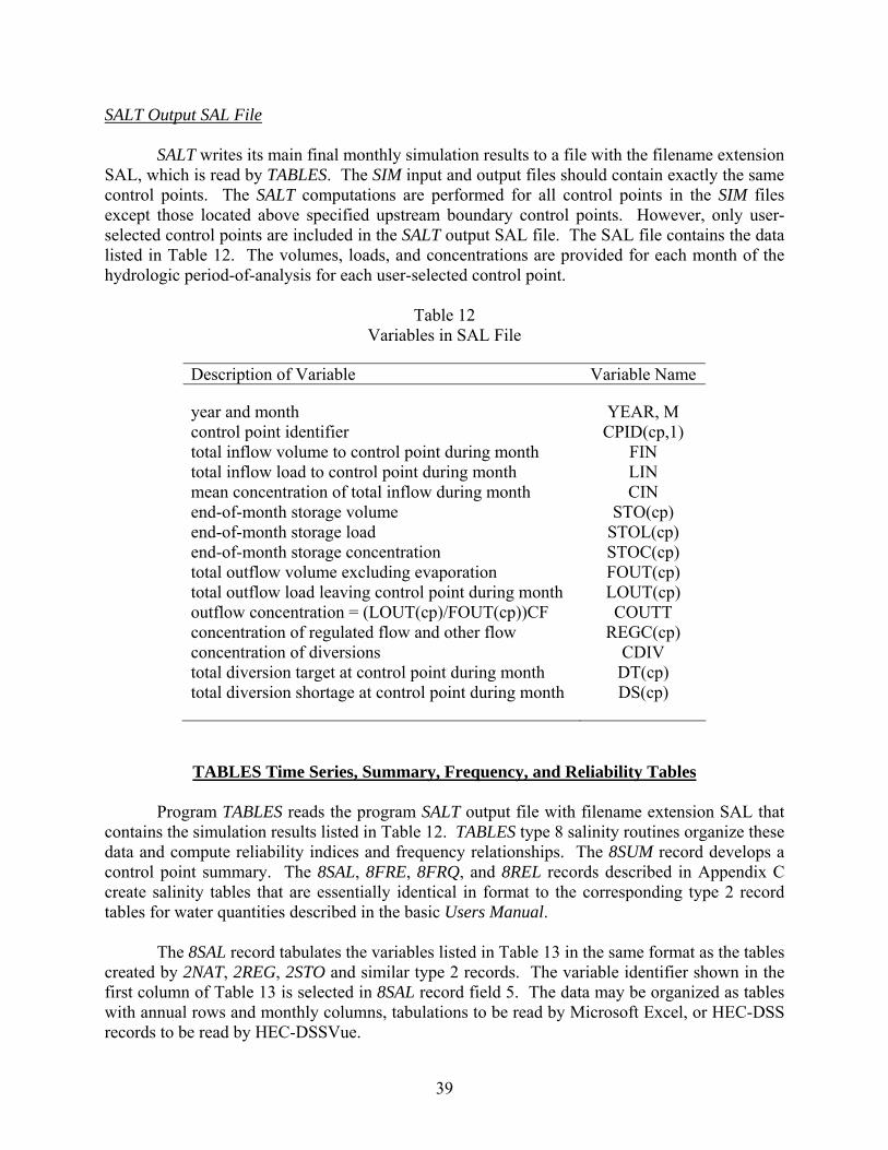
• A SIM/SIMD BRS file provides beginning-of-simulation reservoir storage contents. Program SALT reads salinity input data from a required SIN file and optional BRC file. The salinity input file with filename extension SIN contains the SC, CO, CP, CC, RC, and S records described in Appendix A. The optional beginning reservoir concentration file (extension BRC) may be used to provide beginning-of-simulation storage concentrations. SALT also writes end-of-simulation reservoir concentrations to the BRC file if so specified on the SC record. Program SALT produces output files with filename extensions SAL, SMS, and BRC.

1. The final simulation results output file with filename extension SAL is a table with each line containing the year, month, and control point and the following results for the control point: inflow volume, load, and concentration; end-of-month storage volume, load, and concentration; outflow volume, load, and concentration; downstream flow and diversion concentrations; and diversion target and shortage. Program TABLES reads the SAL file and reorganizes the salinity simulation results in various formats including time series, frequency, and reliability tables.

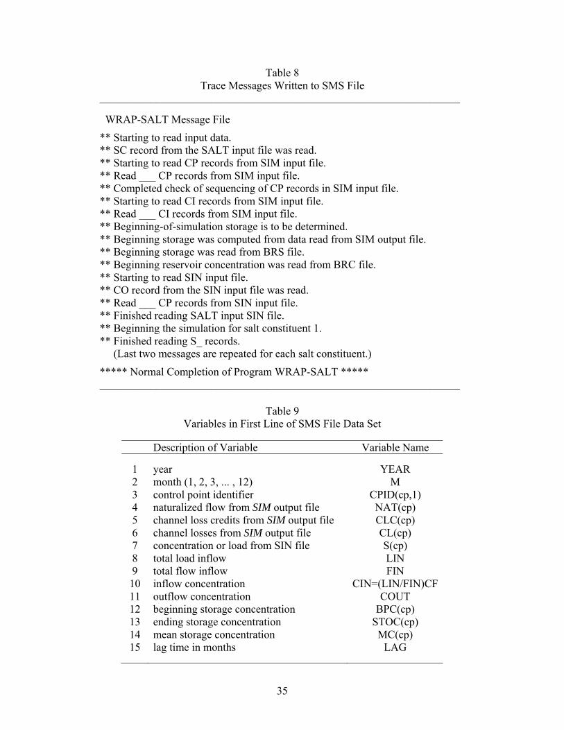
2. The message file with filename extension SMS provides a trace of the simulation,

error and warning messages, an optional listing of control point information, and three types of optional tables of simulation results.

4

3. An optional beginning reservoir concentration file with filename extension BRC contains the final storage concentrations at the end of a simulation to be read by a subsequent execution of SALT as beginning-of-simulation storage concentrations.

The program TABLES reads the program SALT output SAL file with the simulation results and the TABLES input TIN file with specifications regarding the tables to be created. TABLES develops the following tables summarizing the SALT simulation results.

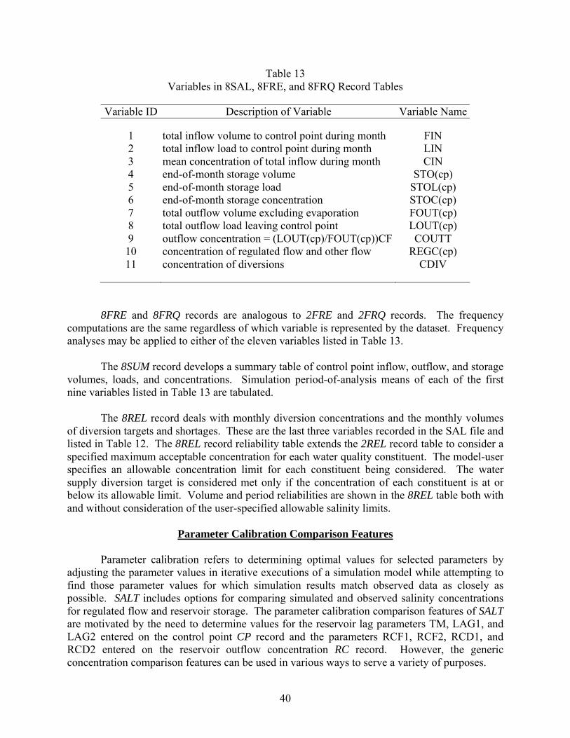
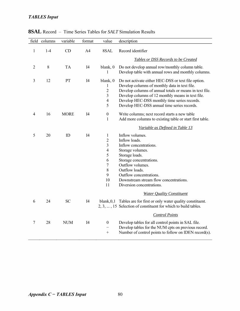
8SAL records create tables of volumes, loads, and concentrations for control point inflow, storage, and outflow that are identical in format to the 2NAT, 2STO, and 2REG, and other type 2 time series tables.

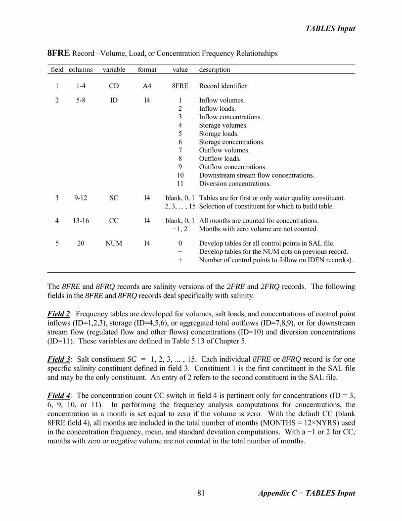
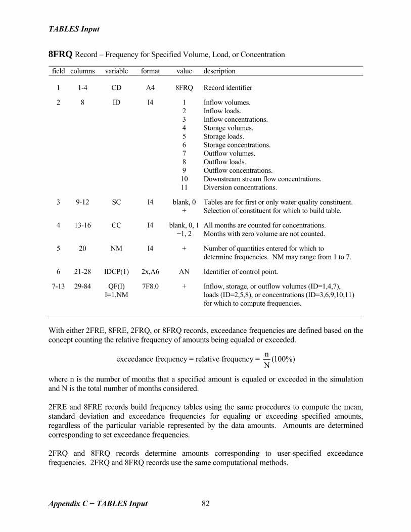
8FRE and 8FRQ records create frequency tables of volumes, loads, and concentrations

for control point inflow, storage, and outflow that are identical in format to the 2FRE and 2FRQ records.

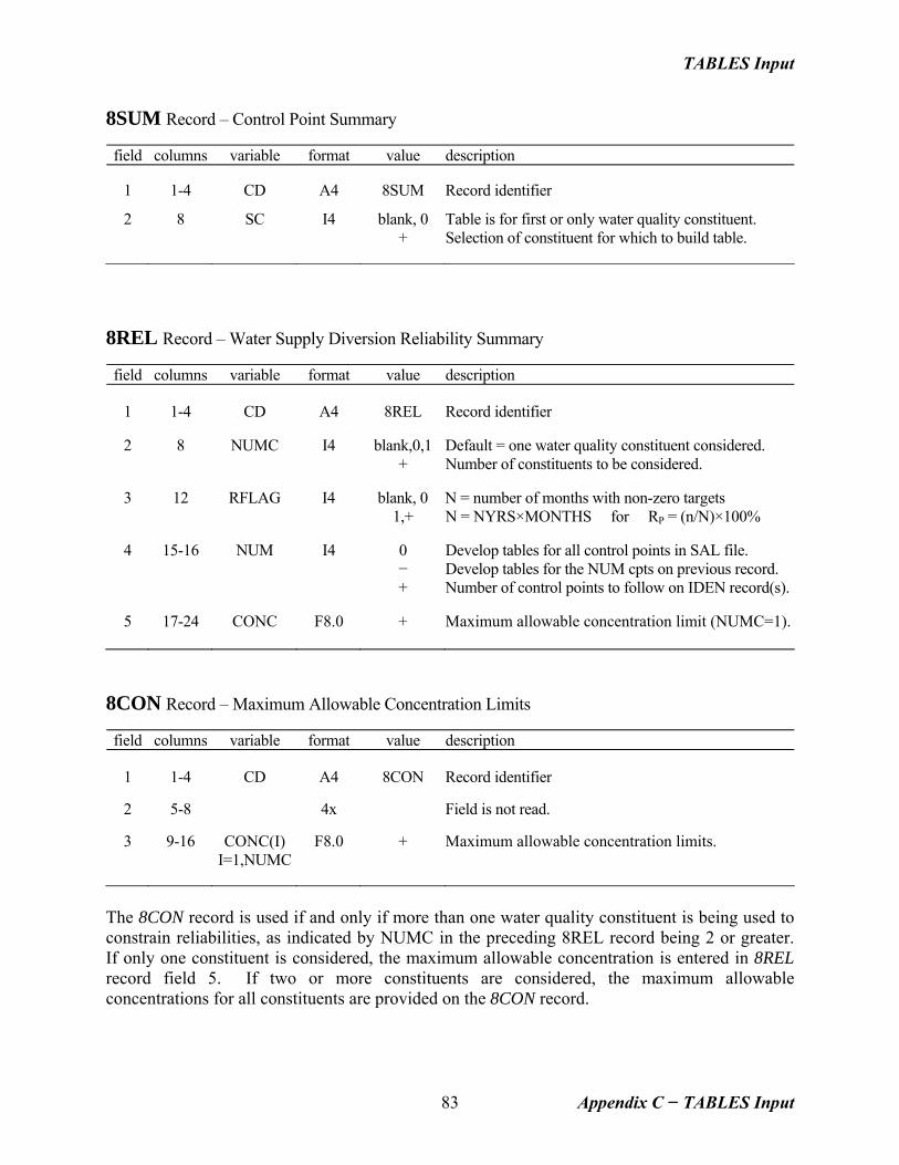
8REL records create reliability tables that reflect limits on salt concentrations. In

addition to the diversion shortages incurred in SIM/SIMD due to insufficient water volume, shortages are declared if concentrations exceed specified levels.

8SUM records provide control point summaries of volumes, loads, and concentrations.

Other optional types of tables recorded by program SALT in the message SMS file do not involve program TABLES. The SMS file tables include:

• listing of control points in sequential order of the computations with pertinent information

• lengthy detailed tabulation of intermediate computation results by time step and control point

• tabulation of simulation results by time step and control point showing details of reservoir lag computations

• brief overall water volume and salt load balance summary table

Spatial Configuration The SIM output OUT file read by SALT must contain output records for all control points included in the SIM input DAT file. The spatial connectivity of a river system is specified by CP records in the SIM DAT file. SALT reads the identifiers of each control point and its next downstream control point from the CP records in the DAT file. A salinity simulation involves two other additional considerations related to the spatial configuration of the river system.

1. SALT performs its salt load tracking computations by control point in an upstream-to-downstream order. All SIM control points must be included in the OUT file.

2. SALT obtains information from CP records found in both the SIN and DAT files. However, the CP records in the SIN file providing salinity data may be fewer in number than the CP records in the DAT file establishing the spatial connectivity of the river system. Salinity input may be repeated for any number of control points.

5

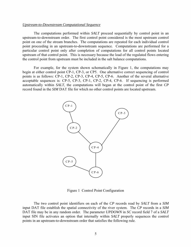
Upstream-to-Downstream Computational Sequence The computations performed within SALT proceed sequentially by control point in an upstream-to-downstream order. The first control point considered is the most upstream control point on one of the stream branches. The computations are repeated for each individual control point proceeding in an upstream-to-downstream sequence. Computations are performed for a particular control point only after completion of computations for all control points located upstream of that control point. This is necessary because the load of the regulated flows entering the control point from upstream must be included in the salt balance computations. For example, for the system shown schematically in Figure 1, the computations may begin at either control point CP-1, CP-3, or CP5. One alternative correct sequencing of control points is as follows: CP-1, CP-2, CP-3, CP-4, CP-5, CP-6. Another of the several alternative acceptable sequences is: CP-5, CP-3, CP-1, CP-2, CP-4, CP-6. If sequencing is performed automatically within SALT, the computations will began at the control point of the first CP record found in the SIM DAT file for which no other control points are located upstream.

C P -1

C P -2

C P -3

C P -4

C P -6

C P -5

Figure 1 Control Point Configuration The two control point identifiers on each of the CP records read by SALT from a SIM input DAT file establish the spatial connectivity of the river system. The CP records in a SIM DAT file may be in any random order. The parameter UPDOWN in SC record field 7 of a SALT input SIN file activates an option that internally within SALT properly sequences the control points in an upstream-to-downstream order that satisfies the following rule.

6

For each control point, all control points located upstream are listed before that control point.

SALT develops an array of control point identifiers that defines the computational sequence. This SALT SC record option is not required if the SIM control point CP records are properly sequenced in the DAT file in accordance with the above rule.

CP records in a SIM or SIMD DAT file can be easily rearranged manually for small datasets with relatively few control points. For larger datasets, the TABLES 1CPT record routine is useful for rearranging CP records with the proper sequencing required for a SALT simulation. With a 1CPT record, program TABLES reads the SIM input DAT file and rearranges the CP records in an appropriate upstream-to-downstream order. The rearranged CP records may then inserted by the model user into a SIM input DAT file to be read by both SIM and SALT. Alternatively, the SC record field 7 option automatically handles the sequencing computationally within the SALT simulation. CP Records in the DAT and SIN Files and Repetition of Salinity Input Data Control point CP records are included in the SALT input SIN file as well as in the SIM input DAT file. The SIN file CP records may be entered in any order. All control points with CP records in the SIN file must also have CP records in the SIM DAT file. However, all control points with CP records in the SIM DAT file do not necessarily have CP records in the SIN file. Certain pertinent information provided for a CP record control point in the SIN file may be repeated for any number of other control points located either upstream or downstream.

Time series of monthly concentrations of local incremental inflows are provided in the SALT salinity input SIN file for any number of control points. Alternatively, a constant concentration rather than monthly varying concentrations for a control point may be specified. The concentrations of incremental inflows read from the SIN file for a particular control point may be repeated for any number of other control points. These data may be provided in the SIN file for any or all of the control points. The data must be included for either the most downstream control point or the most upstream control point on each branch for which salinity is modeled.

Options also allow upstream salinity boundary conditions to be defined at control points that are not upstream extremities. Salinity is not modeled by SALT at control points located upstream of a upstream boundary condition control point even though water quantities are computed in the SIM simulation.

Again using the Figure 1 example, if salinity is to be modeled at all control points, the

SALT input SIN file must include CP records with pertinent salt information for either CP-6 or for CP-1, CP-3, and CP-5. If salinity at CP-1 is not of concern, CP-2 may serve as upstream boundary with CP-1 being omitted from the SIN file. With CP-2 defined as an upstream boundary, salt loads or concentrations for outflows at CP-2 are provided as input in the SIN file. SIM water quantities for CP-1 are read but salinity computations begin at CP-2.

Options in SALT also allow certain salinity data from the SIN file to be repeated for

multiple control points. Assume that the SIM DAT file CP record sequence for the system of

7

Figure 1 is CP-1, CP-2, CP-3, CP-4, CP-5, CP-6. Any or all but at least one of these control points must be included in the SALT SIN file. Repeat options activated by SC record field 11 allow data to be repeated for either upstream (option 1) or downstream (option 2) control points. With option 1, the input data are repeated for all upstream control points not included in the SIN file up to the next control point which is included in the SIN file. For example, with option 1, the concentration of local incremental flows and beginning-of-simulation reservoir storage concentration may provided as input in the SIN file for CP-6 and automatically repeated within SALT for all of the other control points. With option 2, CP-1, CP-3, and CP-5 could be included in the SIN file with repeats occurring as follows. Data input for CP-1 are repeated for CP-2. Input for CP-3 are repeated for CP-4. The data for CP-5 are repeated for CP-6.

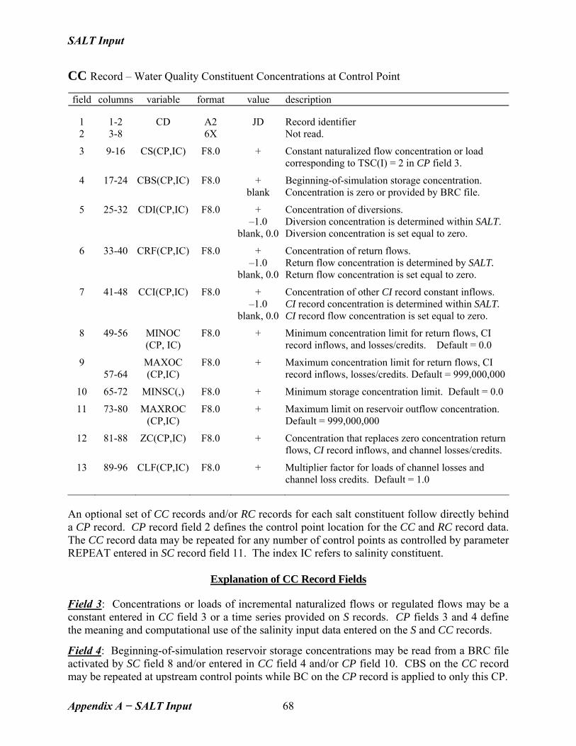
Salinity Input Dataset A WRAP-SALT simulation consists of tracking beginning-of-simulation storage loads and the loads entering the river/reservoir system each month. The SALT salinity input SIN file includes specification of salinity inflows at all control points in the river/reservoir system being modeled. As discussed in the previous section, the salinity inflow data recorded in the SIN file for a particular control point can be automatically repeated within the SALT simulation computations for any number of other control points. The salinity inflows at a particular control point may be provided in the SIN file, as specified by CP record field 3, as either:

1. a time series of concentrations or loads entered as a set of S records 2. a constant concentration or load entered on a CC record 3. zero concentration and load

The salinity inflow data provided on CC and S records may be of the following alternative forms as specified by CP record field 4:

1. concentrations of incremental naturalized flows (The incremental flows are total flows for a control point with no other control points located upstream.)

2. incremental loads (The incremental loads are total loads for a control point with no other control points located upstream.)

3. total loads at an upstream boundary 4. concentrations of total regulated flows at an upstream boundary

Upstream salinity boundary conditions may be defined at control points that are not

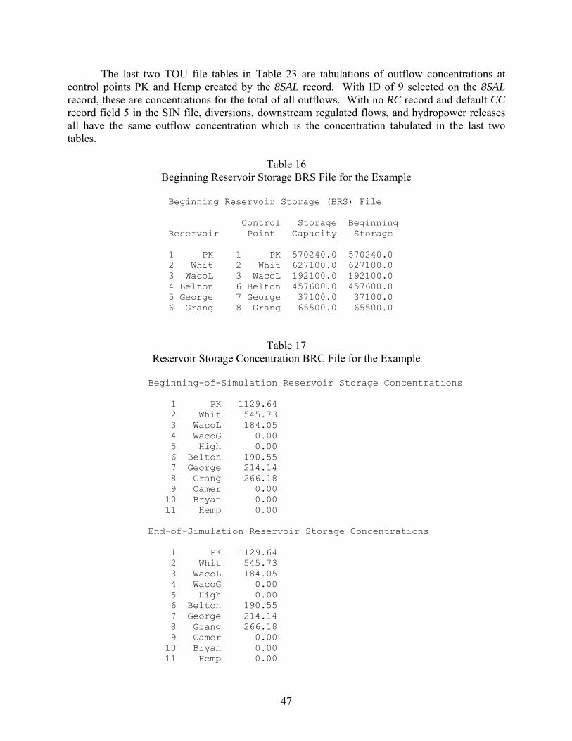
upstream extremities in the SIM dataset. Salinity is not modeled by SALT at control points located upstream of a upstream boundary condition control point even though water quantities are computed in the SIM simulation. All control points must still be included in the SIM output OUT file read by SALT to obtain the correct regulated flow volumes at the upstream salinity boundary, even though the salinity computations begin at the boundary and proceed downstream. Reservoir storage concentrations are specified for the beginning of the simulation period-of-analysis. A beginning concentration may be entered in CC record field 4. Alternatively, a beginning reservoir storage (BRC) file option may be activated by SC record field 9. The storage concentration at the end of the simulation may be recorded in the BRC file for each control point. The storage concentrations at the beginning of the simulation may be read from the BRC file. Beginning concentrations may be manually set equal to ending concentrations.

8

Program SALIN

The availability of salinity data will vary greatly with different river basins and WRAP-SALT applications. Program SALT provides flexible capabilities for specifying salinity inflows to a river/reservoir system in various formats as outlined in the preceding section. Program SALIN is a utility program designed to assist in developing time series of salinity loads or concentrations for inclusion in a SALT input SIN file as S records. Depending upon data availability and options selected for the SALT simulation, the optional SALIN pre-simulation program may possibly be useful in developing the SIN file for a particular application. Instructions for preparing SALIN input data are provided in Appendix B. Program SALIN provides capabilities for extending the time period covered by the salt concentrations or loads recorded on the SIN file S records. For example, Wurbs and Lee (2009) describe a SALT simulation performed for a period-of-analysis of January 1940 through December 2007. Naturalized monthly flow volumes are available for the entire 1940-2007 hydrologic period-of-analysis. However, salinity data are available for only the period from October 1963 through September 1986. SALIN is applied to synthesize loads or concentrations for January 1940 through September 1963 and for November 1986 through December 2007 based on the salinity data available for October 1963 through September 1986 and the naturalized flow volumes available for the entire 1940-2007 hydrologic period-of-analysis. SALIN also computes summary statistics for comparing given and synthesized data sequences. SALIN provides the following alternative approaches for synthesizing either concentrations or loads to extend the period-of-analysis covered by available salinity data.

• conventional least-squares linear or non-linear regression of monthly load or concentration as a function of flow volume

• direct linear interpolation of a flow volume versus load or concentration table The regression analysis alternative may be advantageous over the direct interpolation alternative from the perspective of providing a better estimate of the expected value of monthly concentration or load for a given monthly volume. However, variations in concentration are lost in the regression approach. The direct interpolation option is advantageous compared to regression from the perspective of better preserving the variability in concentrations. Standard textbook least-squares regression procedures are applied in SALIN to compute the coefficients a and b in the equation:

Y = a Xb

(1) X is the naturalized monthly flow volume. Y denotes either monthly loads or concentrations. The linear regression option sets the exponent b at 1.0. The nonlinear regression option allows b to deviate from 1.0. In the previously mentioned example, the coefficients a and b are computed based on the available monthly data for October 1963 through September 1986. Equation 1 is then applied to synthesize loads or concentrations (Y) for the remainder of the 1940-2007 period-of-analysis based on the known naturalized flow volumes (Y). The linear correlation coefficient is also computed as an index of closeness-of-fit.

9

The volume-load table interpolation option consists of the following steps or variations thereof.

1. Again using the previously noted example for illustration, the pairs of flow volumes and loads for the 276 months from October 1963 through September 1986 are ranked in ascending order of flow volume to develop a volume versus load table (array).

2. Linear interpolation of this table is applied to obtain loads corresponding to known naturalized flow volumes for each month of the remainder of the 1940-2007 period.

3. The 1940-2007 monthly loads and volumes are combined to obtain concentrations. Tables of statistics for the flow volumes, loads, and concentrations are developed by SALIN for pertinent time periods to facilitate comparison of synthesized and given data. The statistics include mean, standard deviation, minimum, maximum, and autocorrelation coefficient.

Volumes, Loads, and Concentrations The program SIM simulation results provide volume/month flow rates and end-of-month storage volumes. The program SALT input SIN file provides loads or concentrations for beginning-of-simulation reservoir storage and monthly incremental naturalized stream flows. SALT computes loads and concentrations for inflows, outflows, and storage at all control points except those located upstream of optionally defined upstream boundary control points. Program TABLES salinity routines build tables for volumes, loads, and concentrations for control point inflows, outflows, and storage. TABLES also has a routine for determining water supply diversion reliabilities constrained by maximum allowable salt concentration limits. Units of Measure

Any consistent set of units may be adopted for storage volumes, volume/month flow rates, salt loads, and concentrations. A conversion factor may be entered in SC record field 15 to set the unit of measure for concentration for given load and volume units. Concentration (C), load (L), and storage or flow volume (Q) are related as follows:

CC

L CQC = f L =Q f

or

(2)

where fC is a conversion factor that is entered in SC record field 15, with a default of 735.48 that corresponds to units of milligrams per liter (mg/l) for C, tons or tons/month for L, and acre-feet or acre-feet/month for Q. The default factor reflects the following conversions. 3

3mg tons 2,000pounds 453.59g 1,000mg ac-ft ft=liter ac-ft ton pound gram 28.316 liters43,560ft

⎛ ⎞⎛ ⎞⎛ ⎞⎛ ⎞⎛ ⎞⎛ ⎞ ⎜ ⎟⎜ ⎟⎜ ⎟⎜ ⎟⎜ ⎟⎜ ⎟ ⎜ ⎟⎜ ⎟⎝ ⎠⎝ ⎠⎝ ⎠⎝ ⎠⎝ ⎠⎝ ⎠

( )milligrams tons= 735.48liter acre-feet

⎛ ⎞⎜ ⎟⎝ ⎠

10

For units of mg/l, tons/day, and ft3/s, the conversion factor fC = 370.81 should be entered in SC record field 15.

3

3mg tons/day 2,000pounds 453.59g 1,000mg day ft=liter ton pound gram 86,400s 28.316 litersft /s

⎛ ⎞⎛ ⎞⎛ ⎞⎛ ⎞⎛ ⎞⎛ ⎞ ⎜ ⎟⎜ ⎟⎜ ⎟⎜ ⎟⎜ ⎟⎜ ⎟ ⎜ ⎟⎝ ⎠⎝ ⎠ ⎝ ⎠⎝ ⎠⎝ ⎠⎝ ⎠

( )3milligrams tons/day= 370.81

liter ft / s⎛ ⎞⎜ ⎟⎝ ⎠

Discharge-weighted or volume-weighed mean concentrations CM are computed as follows.

M C

LC = fQΣΣ

(3)

The concentrations of monthly flows entering the confluence of two tributaries are combined to obtain the discharge-weighted mean concentration of flow leaving the confluence. Likewise, monthly loads and flows are summed to obtain a discharge-weighted mean annual concentration. Components of Control Point Inflows and Outflows The following volume and load balance equations are fundamental to the WRAP-SALT simulation computations. change in reservoir storage volume = inflow volume – outflow volume (4) change in reservoir storage load = inflow load – outflow load (5) Equations 4 and 5 are applied at each control point for each month of the simulation. For control points with no reservoirs, storage volume and load are zero. For the volume and load balance summary table written to the message SMS file, Equations 4 and 5 are applicable to the total river/reservoir system over the total period-of-analysis. The volume and load balances are actually applicable to any contiguous set of control points over any period of time. From the perspective of volume and load balances at a control point, the inflow and outflow terms in Eqs. 4 and 5 consist of the summation of the inflow and outflow components listed in Table 1. Monthly volumes of naturalized flow, regulated flow, end-of-month reservoir storage, channel loss credits, channel losses, and return flows are read by SALT from the SIM output file and are defined in the Reference and Users Manuals. Monthly diversion targets and shortages are also read from the SIM output file, and diversion volumes are computed as their difference. Constant inflows input to SIM on CI records are not included as separate quantities in the SIM output file. Thus, SALT reads the CI records from the SIM input file along with the CP records. The inflow and outflow volumes and loads written to the SAL output file are the totals for the component inflows and outflows listed in Table 1. The inflow and outflow concentrations are the volume-weighted means of the concentrations of each component.

11

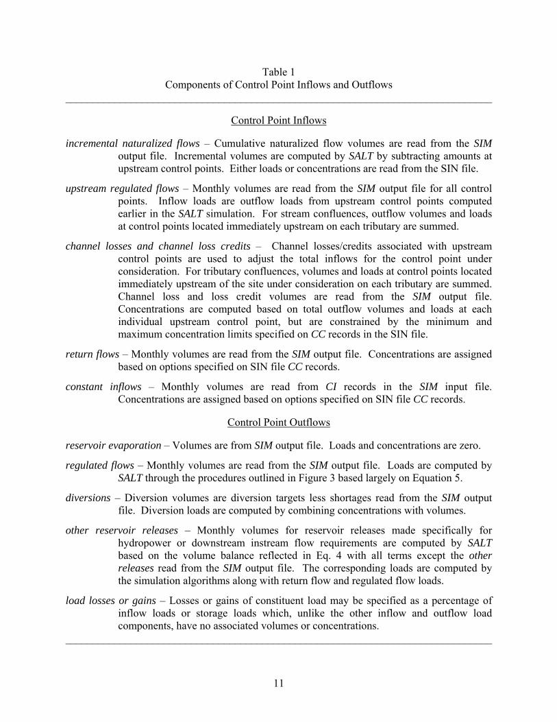
Table 1 Components of Control Point Inflows and Outflows

______________________________________________________________________________

Control Point Inflows incremental naturalized flows – Cumulative naturalized flow volumes are read from the SIM

output file. Incremental volumes are computed by SALT by subtracting amounts at upstream control points. Either loads or concentrations are read from the SIN file.

upstream regulated flows – Monthly volumes are read from the SIM output file for all control points. Inflow loads are outflow loads from upstream control points computed earlier in the SALT simulation. For stream confluences, outflow volumes and loads at control points located immediately upstream on each tributary are summed.

channel losses and channel loss credits – Channel losses/credits associated with upstream control points are used to adjust the total inflows for the control point under consideration. For tributary confluences, volumes and loads at control points located immediately upstream of the site under consideration on each tributary are summed. Channel loss and loss credit volumes are read from the SIM output file. Concentrations are computed based on total outflow volumes and loads at each individual upstream control point, but are constrained by the minimum and maximum concentration limits specified on CC records in the SIN file.

return flows – Monthly volumes are read from the SIM output file. Concentrations are assigned based on options specified on SIN file CC records.

constant inflows – Monthly volumes are read from CI records in the SIM input file. Concentrations are assigned based on options specified on SIN file CC records.

Control Point Outflows

reservoir evaporation – Volumes are from SIM output file. Loads and concentrations are zero.

regulated flows – Monthly volumes are read from the SIM output file. Loads are computed by SALT through the procedures outlined in Figure 3 based largely on Equation 5.

diversions – Diversion volumes are diversion targets less shortages read from the SIM output file. Diversion loads are computed by combining concentrations with volumes.

other reservoir releases – Monthly volumes for reservoir releases made specifically for hydropower or downstream instream flow requirements are computed by SALT based on the volume balance reflected in Eq. 4 with all terms except the other releases read from the SIM output file. The corresponding loads are computed by the simulation algorithms along with return flow and regulated flow loads.

load losses or gains – Losses or gains of constituent load may be specified as a percentage of inflow loads or storage loads which, unlike the other inflow and outflow load components, have no associated volumes or concentrations.

______________________________________________________________________________

12

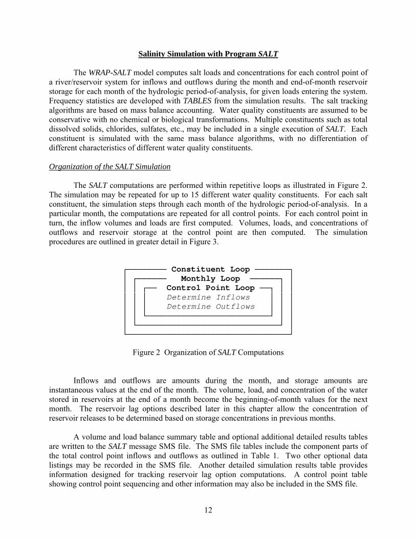
Salinity Simulation with Program SALT The WRAP-SALT model computes salt loads and concentrations for each control point of a river/reservoir system for inflows and outflows during the month and end-of-month reservoir storage for each month of the hydrologic period-of-analysis, for given loads entering the system. Frequency statistics are developed with TABLES from the simulation results. The salt tracking algorithms are based on mass balance accounting. Water quality constituents are assumed to be conservative with no chemical or biological transformations. Multiple constituents such as total dissolved solids, chlorides, sulfates, etc., may be included in a single execution of SALT. Each constituent is simulated with the same mass balance algorithms, with no differentiation of different characteristics of different water quality constituents. Organization of the SALT Simulation The SALT computations are performed within repetitive loops as illustrated in Figure 2. The simulation may be repeated for up to 15 different water quality constituents. For each salt constituent, the simulation steps through each month of the hydrologic period-of-analysis. In a particular month, the computations are repeated for all control points. For each control point in turn, the inflow volumes and loads are first computed. Volumes, loads, and concentrations of outflows and reservoir storage at the control point are then computed. The simulation procedures are outlined in greater detail in Figure 3.

┌──────── Constituent Loop ───────┐ │ ┌────── Monthly Loop ──────┐ │ │ │ ┌── Control Point Loop ──┐ │ │ │ │ │ Determine Inflows │ │ │ │ │ │ Determine Outflows │ │ │ │ │ └─────────────────────────┘ │ │ │ └─────────────────────────────┘ │ └─────────────────────────────────┘

Figure 2 Organization of SALT Computations

Inflows and outflows are amounts during the month, and storage amounts are instantaneous values at the end of the month. The volume, load, and concentration of the water stored in reservoirs at the end of a month become the beginning-of-month values for the next month. The reservoir lag options described later in this chapter allow the concentration of reservoir releases to be determined based on storage concentrations in previous months.

A volume and load balance summary table and optional additional detailed results tables are written to the SALT message SMS file. The SMS file tables include the component parts of the total control point inflows and outflows as outlined in Table 1. Two other optional data listings may be recorded in the SMS file. Another detailed simulation results table provides information designed for tracking reservoir lag option computations. A control point table showing control point sequencing and other information may also be included in the SMS file.

13

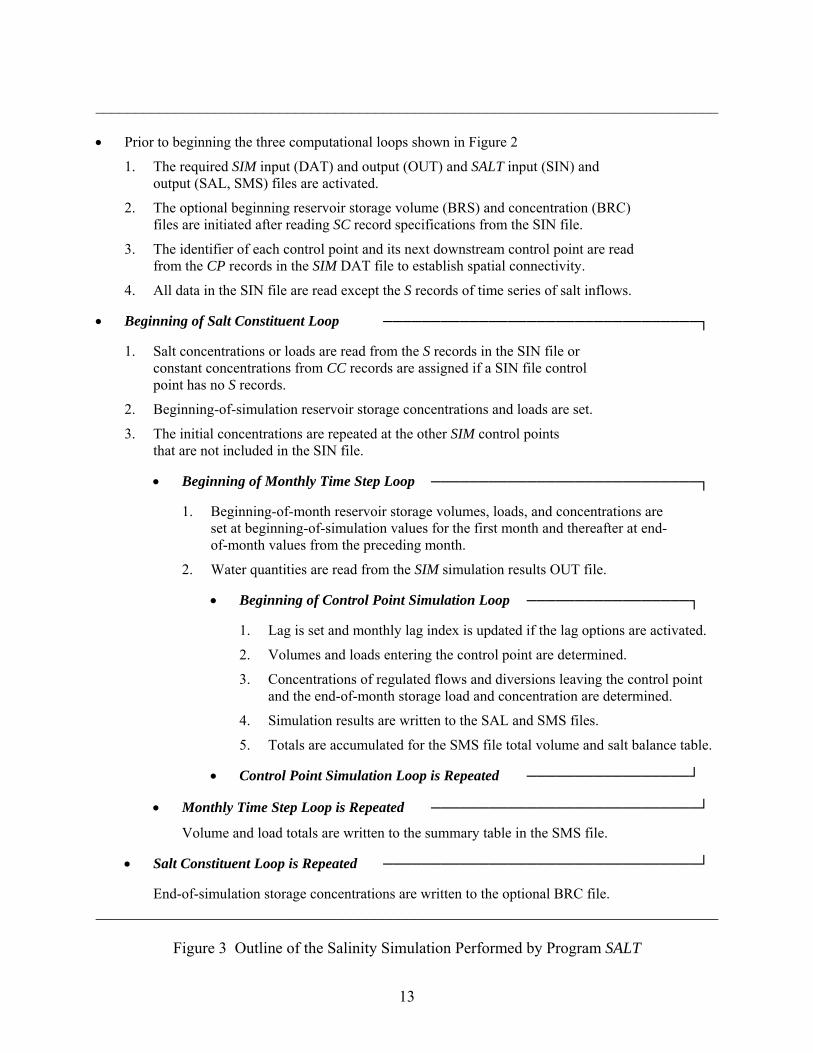
______________________________________________________________________________ • Prior to beginning the three computational loops shown in Figure 2

1. The required SIM input (DAT) and output (OUT) and SALT input (SIN) and output (SAL, SMS) files are activated.

2. The optional beginning reservoir storage volume (BRS) and concentration (BRC) files are initiated after reading SC record specifications from the SIN file.

3. The identifier of each control point and its next downstream control point are read from the CP records in the SIM DAT file to establish spatial connectivity.

4. All data in the SIN file are read except the S records of time series of salt inflows.

• Beginning of Salt Constituent Loop ─────────────────────────────────┐

1. Salt concentrations or loads are read from the S records in the SIN file or constant concentrations from CC records are assigned if a SIN file control point has no S records.

2. Beginning-of-simulation reservoir storage concentrations and loads are set.

3. The initial concentrations are repeated at the other SIM control points that are not included in the SIN file.

• Beginning of Monthly Time Step Loop ────────────────────────────┐

1. Beginning-of-month reservoir storage volumes, loads, and concentrations are set at beginning-of-simulation values for the first month and thereafter at end- of-month values from the preceding month.

2. Water quantities are read from the SIM simulation results OUT file.

• Beginning of Control Point Simulation Loop ─────────────────┐

1. Lag is set and monthly lag index is updated if the lag options are activated.

2. Volumes and loads entering the control point are determined.

3. Concentrations of regulated flows and diversions leaving the control point and the end-of-month storage load and concentration are determined.

4. Simulation results are written to the SAL and SMS files.

5. Totals are accumulated for the SMS file total volume and salt balance table.

• Control Point Simulation Loop is Repeated ─────────────────┘

• Monthly Time Step Loop is Repeated ────────────────────────────┘

Volume and load totals are written to the summary table in the SMS file.

• Salt Constituent Loop is Repeated ─────────────────────────────────┘ End-of-simulation storage concentrations are written to the optional BRC file.

______________________________________________________________________________

Figure 3 Outline of the Salinity Simulation Performed by Program SALT

14

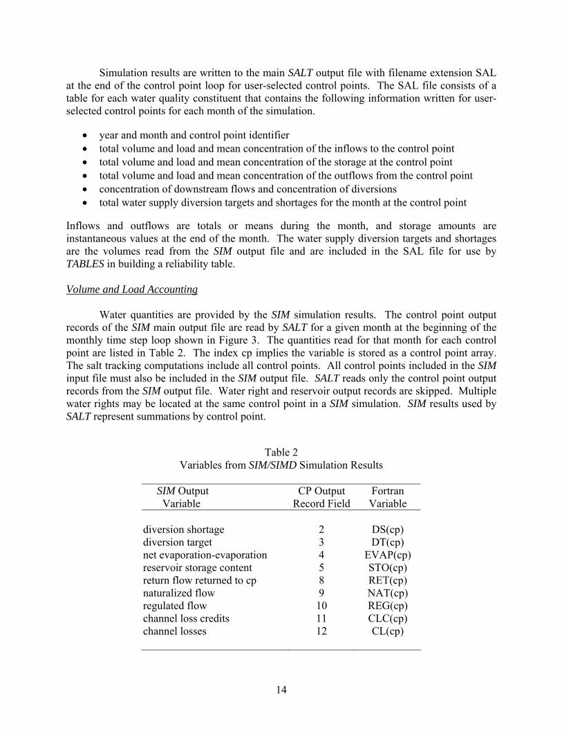
Simulation results are written to the main SALT output file with filename extension SAL at the end of the control point loop for user-selected control points. The SAL file consists of a table for each water quality constituent that contains the following information written for user-selected control points for each month of the simulation.

• year and month and control point identifier • total volume and load and mean concentration of the inflows to the control point • total volume and load and mean concentration of the storage at the control point • total volume and load and mean concentration of the outflows from the control point • concentration of downstream flows and concentration of diversions • total water supply diversion targets and shortages for the month at the control point

Inflows and outflows are totals or means during the month, and storage amounts are instantaneous values at the end of the month. The water supply diversion targets and shortages are the volumes read from the SIM output file and are included in the SAL file for use by TABLES in building a reliability table. Volume and Load Accounting

Water quantities are provided by the SIM simulation results. The control point output records of the SIM main output file are read by SALT for a given month at the beginning of the monthly time step loop shown in Figure 3. The quantities read for that month for each control point are listed in Table 2. The index cp implies the variable is stored as a control point array. The salt tracking computations include all control points. All control points included in the SIM input file must also be included in the SIM output file. SALT reads only the control point output records from the SIM output file. Water right and reservoir output records are skipped. Multiple water rights may be located at the same control point in a SIM simulation. SIM results used by SALT represent summations by control point.

Table 2 Variables from SIM/SIMD Simulation Results

SIM Output CP Output Fortran Variable Record Field Variable diversion shortage 2 DS(cp) diversion target 3 DT(cp) net evaporation-evaporation 4 EVAP(cp) reservoir storage content 5 STO(cp) return flow returned to cp 8 RET(cp) naturalized flow 9 NAT(cp) regulated flow 10 REG(cp) channel loss credits 11 CLC(cp) channel losses 12 CL(cp)

15

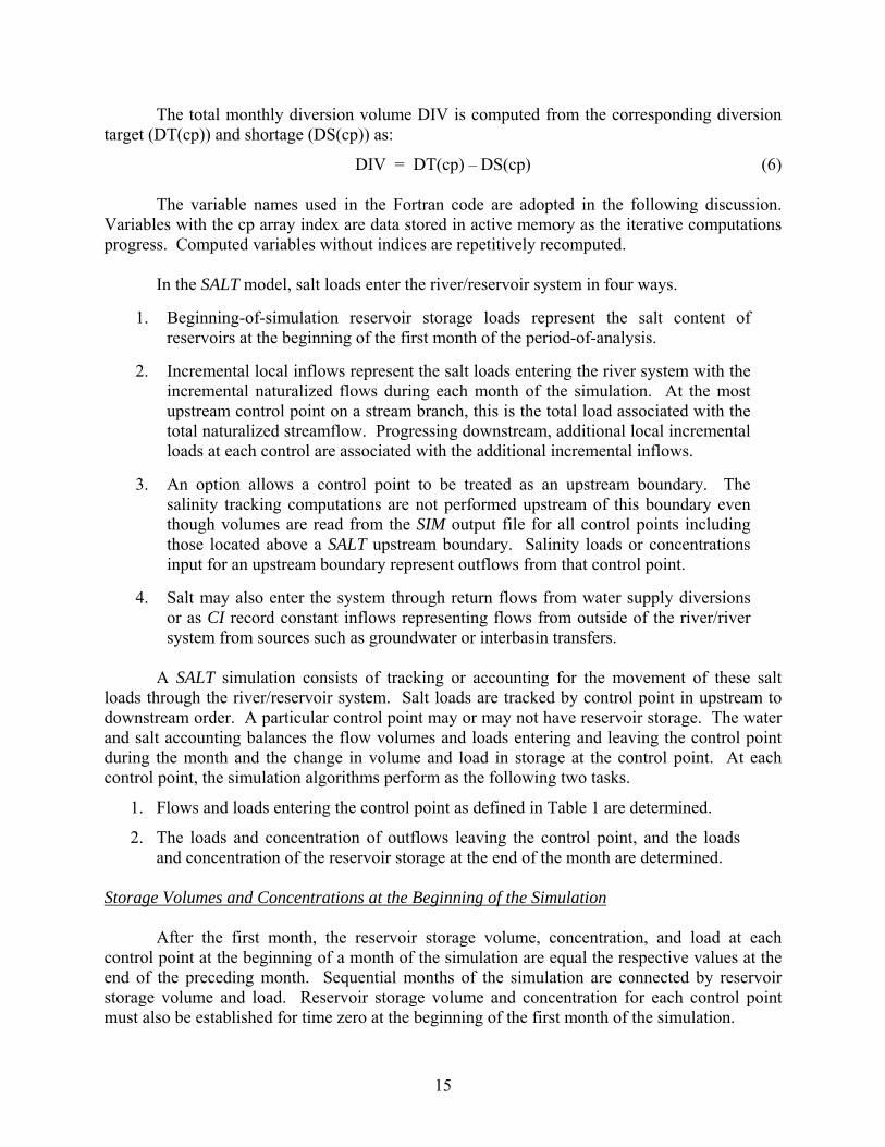
The total monthly diversion volume DIV is computed from the corresponding diversion target (DT(cp)) and shortage (DS(cp)) as:

DIV = DT(cp) – DS(cp) (6) The variable names used in the Fortran code are adopted in the following discussion. Variables with the cp array index are data stored in active memory as the iterative computations progress. Computed variables without indices are repetitively recomputed. In the SALT model, salt loads enter the river/reservoir system in four ways.

1. Beginning-of-simulation reservoir storage loads represent the salt content of reservoirs at the beginning of the first month of the period-of-analysis.

2. Incremental local inflows represent the salt loads entering the river system with the

incremental naturalized flows during each month of the simulation. At the most upstream control point on a stream branch, this is the total load associated with the total naturalized streamflow. Progressing downstream, additional local incremental loads at each control are associated with the additional incremental inflows.

3. An option allows a control point to be treated as an upstream boundary. The

salinity tracking computations are not performed upstream of this boundary even though volumes are read from the SIM output file for all control points including those located above a SALT upstream boundary. Salinity loads or concentrations input for an upstream boundary represent outflows from that control point.

4. Salt may also enter the system through return flows from water supply diversions

or as CI record constant inflows representing flows from outside of the river/river system from sources such as groundwater or interbasin transfers.

A SALT simulation consists of tracking or accounting for the movement of these salt loads through the river/reservoir system. Salt loads are tracked by control point in upstream to downstream order. A particular control point may or may not have reservoir storage. The water and salt accounting balances the flow volumes and loads entering and leaving the control point during the month and the change in volume and load in storage at the control point. At each control point, the simulation algorithms perform as the following two tasks.

1. Flows and loads entering the control point as defined in Table 1 are determined.

2. The loads and concentration of outflows leaving the control point, and the loads and concentration of the reservoir storage at the end of the month are determined.

Storage Volumes and Concentrations at the Beginning of the Simulation After the first month, the reservoir storage volume, concentration, and load at each control point at the beginning of a month of the simulation are equal the respective values at the end of the preceding month. Sequential months of the simulation are connected by reservoir storage volume and load. Reservoir storage volume and concentration for each control point must also be established for time zero at the beginning of the first month of the simulation.

16

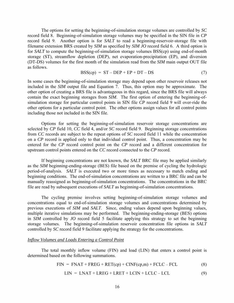
The options for setting the beginning-of-simulation storage volumes are controlled by SC record field 8. Beginning-of-simulation storage volumes may be specified in the SIN file in CP record field 9. Another option is for SALT to read a beginning-reservoir-storage file with filename extension BRS created by SIM as specified by SIM JO record field 6. A third option is for SALT to compute the beginning-of-simulation storage volumes BSS(cp) using end-of-month storage (ST), streamflow depletion (DEP), net evaporation-precipitation (EP), and diversion (DT-DS) volumes for the first month of the simulation read from the SIM main output OUT file as follows. BSS(cp) = ST – DEP + EP + DT – DS (7) In some cases the beginning-of-simulation storage may depend upon other reservoir releases not included in the SIM output file and Equation 7. Thus, this option may be approximate. The other option of creating a BRS file is advantageous in this regard, since the BRS file will always contain the exact beginning storages from SIM. The first option of entering the beginning-of-simulation storage for particular control points in SIN file CP record field 9 will over-ride the other options for a particular control point. The other options assign values for all control points including those not included in the SIN file. Options for setting the beginning-of-simulation reservoir storage concentrations are selected by CP field 10, CC field 4, and/or SC record field 9. Beginning storage concentrations from CC records are subject to the repeat options of SC record field 11 while the concentration on a CP record is applied only to that individual control point. Thus, a concentration may be entered for the CP record control point on the CP record and a different concentration for upstream control points entered on the CC record connected to the CP record.

If beginning concentrations are not known, the SALT BRC file may be applied similarly as the SIM beginning-ending-storage (BES) file based on the premise of cycling the hydrologic period-of-analysis. SALT is executed two or more times as necessary to match ending and beginning conditions. The end-of-simulation concentrations are written to a BRC file and can be manually reassigned as beginning-of-simulation concentrations. The concentrations in the BRC file are read by subsequent executions of SALT as beginning-of-simulation concentrations. The cycling premise involves setting beginning-of-simulation storage volumes and concentrations equal to end-of-simulation storage volumes and concentrations determined by previous executions of SIM and SALT. Since, ending values depend upon beginning values, multiple iterative simulations may be performed. The beginning-ending-storage (BES) options in SIM controlled by JO record field 5 facilitate applying this strategy to set the beginning storage volumes. The beginning-of-simulation reservoir concentration file options in SALT controlled by SC record field 9 facilitate applying the strategy for the concentrations. Inflow Volumes and Loads Entering a Control Point

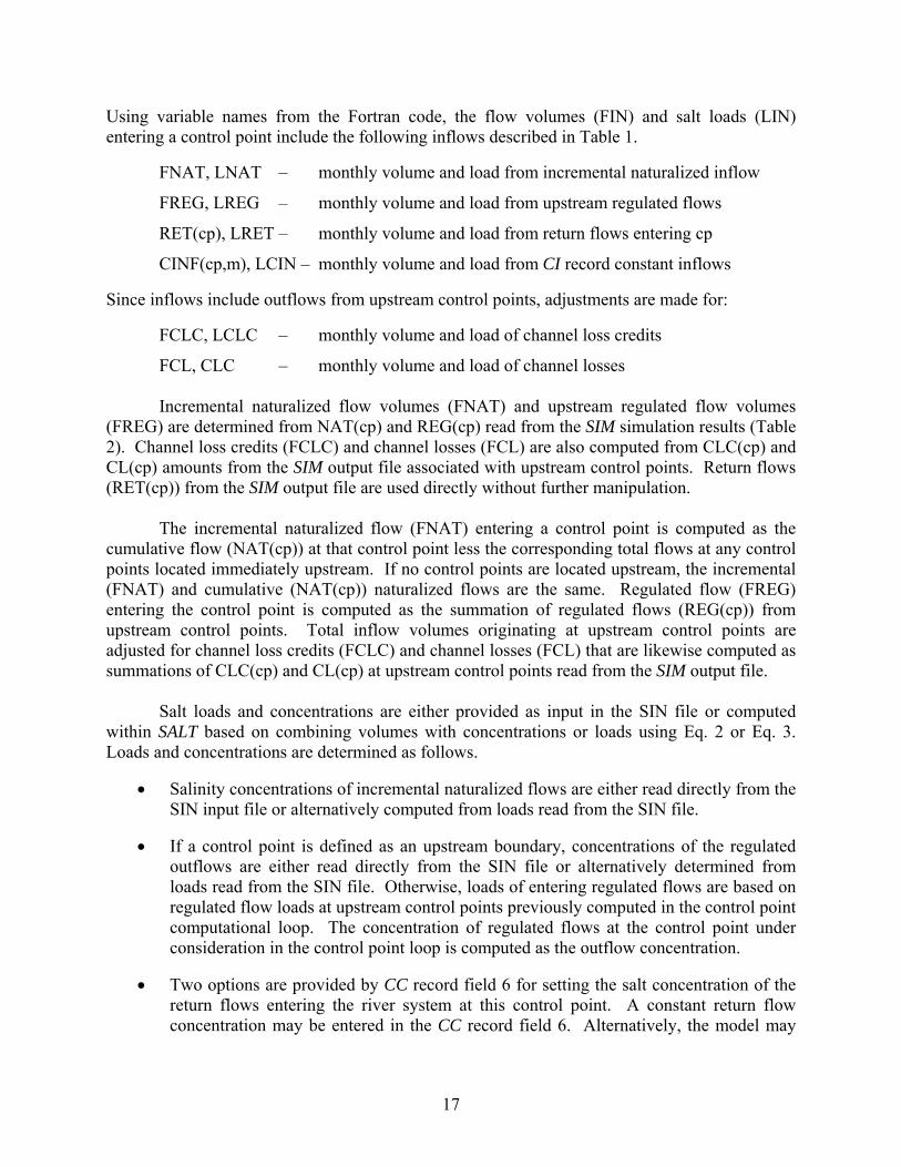
The total monthly inflow volume (FIN) and load (LIN) that enters a control point is determined based on the following summations. FIN = FNAT + FREG + RET(cp) + CINF(cp,m) + FCLC – FCL (8) LIN = LNAT + LREG + LRET + LCIN + LCLC – LCL (9)

17

Using variable names from the Fortran code, the flow volumes (FIN) and salt loads (LIN) entering a control point include the following inflows described in Table 1.

FNAT, LNAT – monthly volume and load from incremental naturalized inflow

FREG, LREG – monthly volume and load from upstream regulated flows

RET(cp), LRET – monthly volume and load from return flows entering cp

CINF(cp,m), LCIN – monthly volume and load from CI record constant inflows Since inflows include outflows from upstream control points, adjustments are made for:

FCLC, LCLC – monthly volume and load of channel loss credits

FCL, CLC – monthly volume and load of channel losses

Incremental naturalized flow volumes (FNAT) and upstream regulated flow volumes (FREG) are determined from NAT(cp) and REG(cp) read from the SIM simulation results (Table 2). Channel loss credits (FCLC) and channel losses (FCL) are also computed from CLC(cp) and CL(cp) amounts from the SIM output file associated with upstream control points. Return flows (RET(cp)) from the SIM output file are used directly without further manipulation.

The incremental naturalized flow (FNAT) entering a control point is computed as the cumulative flow (NAT(cp)) at that control point less the corresponding total flows at any control points located immediately upstream. If no control points are located upstream, the incremental (FNAT) and cumulative (NAT(cp)) naturalized flows are the same. Regulated flow (FREG) entering the control point is computed as the summation of regulated flows (REG(cp)) from upstream control points. Total inflow volumes originating at upstream control points are adjusted for channel loss credits (FCLC) and channel losses (FCL) that are likewise computed as summations of CLC(cp) and CL(cp) at upstream control points read from the SIM output file.

Salt loads and concentrations are either provided as input in the SIN file or computed within SALT based on combining volumes with concentrations or loads using Eq. 2 or Eq. 3. Loads and concentrations are determined as follows.

• Salinity concentrations of incremental naturalized flows are either read directly from the SIN input file or alternatively computed from loads read from the SIN file.

• If a control point is defined as an upstream boundary, concentrations of the regulated

outflows are either read directly from the SIN file or alternatively determined from loads read from the SIN file. Otherwise, loads of entering regulated flows are based on regulated flow loads at upstream control points previously computed in the control point computational loop. The concentration of regulated flows at the control point under consideration in the control point loop is computed as the outflow concentration.

• Two options are provided by CC record field 6 for setting the salt concentration of the

return flows entering the river system at this control point. A constant return flow concentration may be entered in the CC record field 6. Alternatively, the model may

18

adopt the mean concentration of the outflows from upstream control points constrained by the limits specified in CC record fields 8 and 9.

• Two options are provided by CC record field 7 for setting the concentration of the CI

record constant inflows entering the river system at this control point. A constant inflow concentration may be entered in the CC record field 7. Alternatively, SALT may use the mean concentration of the outflows from upstream control points constrained by the limits specified in CC record fields 8 and 9 in the same manner as for return flows.

• Loads of inflows originating from control points located upstream are adjusted for

channel losses and loss credits based on concentrations at individual upstream control points determined from previously computed outflow volumes and loads. The limits from CC record fields 8 and 9 are applied. Estimating loads associated with channel losses/credits also includes application of an optional multiplier factor (CLF) from CC record field 12 that has a default value of 1.0. A CLF of 1.0 means that salt loads and stream flow volumes are lost to channel losses in the same proportion. CLF less than or greater than 1.0 increases or decreases the impact of channel losses on loads.

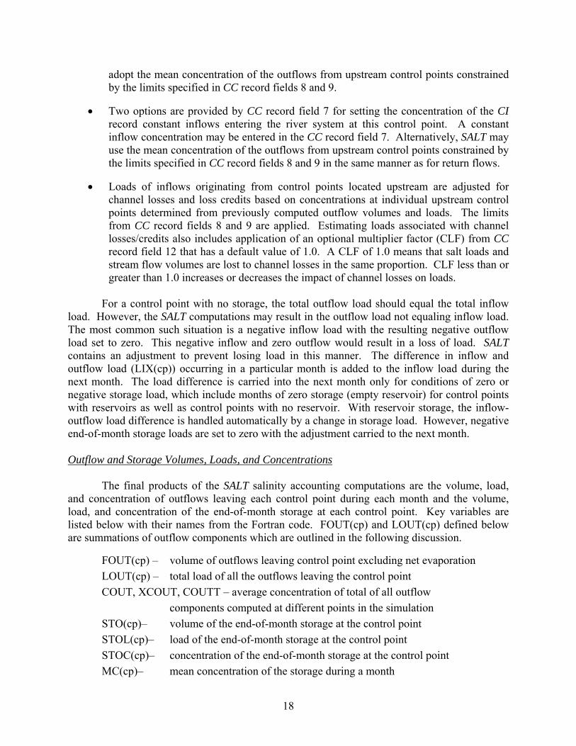
For a control point with no storage, the total outflow load should equal the total inflow load. However, the SALT computations may result in the outflow load not equaling inflow load. The most common such situation is a negative inflow load with the resulting negative outflow load set to zero. This negative inflow and zero outflow would result in a loss of load. SALT contains an adjustment to prevent losing load in this manner. The difference in inflow and outflow load (LIX(cp)) occurring in a particular month is added to the inflow load during the next month. The load difference is carried into the next month only for conditions of zero or negative storage load, which include months of zero storage (empty reservoir) for control points with reservoirs as well as control points with no reservoir. With reservoir storage, the inflow-outflow load difference is handled automatically by a change in storage load. However, negative end-of-month storage loads are set to zero with the adjustment carried to the next month. Outflow and Storage Volumes, Loads, and Concentrations The final products of the SALT salinity accounting computations are the volume, load, and concentration of outflows leaving each control point during each month and the volume, load, and concentration of the end-of-month storage at each control point. Key variables are listed below with their names from the Fortran code. FOUT(cp) and LOUT(cp) defined below are summations of outflow components which are outlined in the following discussion.

FOUT(cp) – volume of outflows leaving control point excluding net evaporation LOUT(cp) – total load of all the outflows leaving the control point COUT, XCOUT, COUTT – average concentration of total of all outflow

components computed at different points in the simulation STO(cp)– volume of the end-of-month storage at the control point STOL(cp)– load of the end-of-month storage at the control point STOC(cp)– concentration of the end-of-month storage at the control point MC(cp)– mean concentration of the storage during a month

19

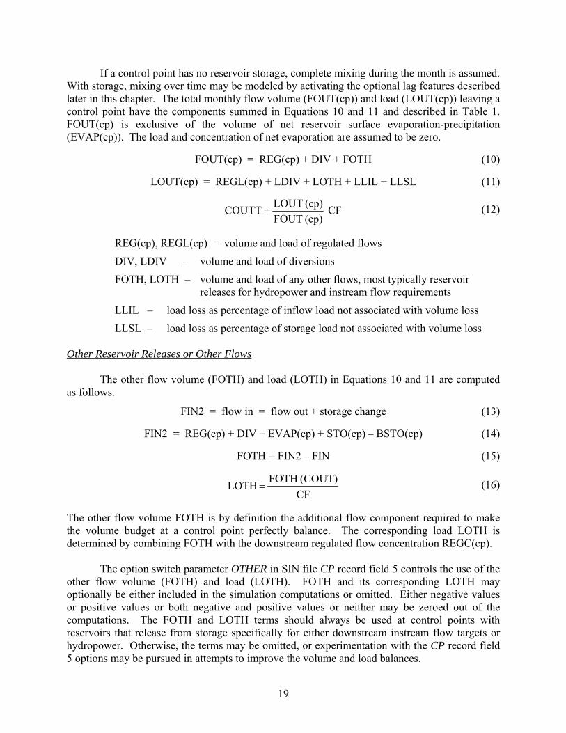
If a control point has no reservoir storage, complete mixing during the month is assumed. With storage, mixing over time may be modeled by activating the optional lag features described later in this chapter. The total monthly flow volume (FOUT(cp)) and load (LOUT(cp)) leaving a control point have the components summed in Equations 10 and 11 and described in Table 1. FOUT(cp) is exclusive of the volume of net reservoir surface evaporation-precipitation (EVAP(cp)). The load and concentration of net evaporation are assumed to be zero. FOUT(cp) = REG(cp) + DIV + FOTH (10) LOUT(cp) = REGL(cp) + LDIV + LOTH + LLIL + LLSL (11)

CF(cp) FOUT(cp) LOUT COUTT =

(12)

REG(cp), REGL(cp) – volume and load of regulated flows

DIV, LDIV – volume and load of diversions

FOTH, LOTH – volume and load of any other flows, most typically reservoir releases for hydropower and instream flow requirements

LLIL – load loss as percentage of inflow load not associated with volume loss

LLSL – load loss as percentage of storage load not associated with volume loss

Other Reservoir Releases or Other Flows The other flow volume (FOTH) and load (LOTH) in Equations 10 and 11 are computed as follows.

FIN2 = flow in = flow out + storage change (13) FIN2 = REG(cp) + DIV + EVAP(cp) + STO(cp) – BSTO(cp) (14) FOTH = FIN2 – FIN (15)

CF(COUT) FOTH LOTH =

(16)

The other flow volume FOTH is by definition the additional flow component required to make the volume budget at a control point perfectly balance. The corresponding load LOTH is determined by combining FOTH with the downstream regulated flow concentration REGC(cp).

The option switch parameter OTHER in SIN file CP record field 5 controls the use of the other flow volume (FOTH) and load (LOTH). FOTH and its corresponding LOTH may optionally be either included in the simulation computations or omitted. Either negative values or positive values or both negative and positive values or neither may be zeroed out of the computations. The FOTH and LOTH terms should always be used at control points with reservoirs that release from storage specifically for either downstream instream flow targets or hydropower. Otherwise, the terms may be omitted, or experimentation with the CP record field 5 options may be pursued in attempts to improve the volume and load balances.

20

The FOTH and LOTH terms model releases made specifically for hydroelectric power generation or releases from storage for meeting instream flow requirements. Passing of reservoir inflows for downstream instream flow requirements and water supply releases that incidentally generate hydropower are not included in this category of other releases. The return flows in the SIM output file include reservoir releases to meet hydropower and instream flow requirements. Effects of return flows are reflected in the SIM regulated flow results. Return flows incorporating these other reservoir releases are included in SALT in the control point inflows. To maintain the volume balance, hydropower and instream flow releases must also be included in the computations in the same way as diversions as quantities in the control point outflows.

SIM negative incremental naturalized flows, SALT negative inflows, and options for

dealing with them (JD record field 8, SC record field 14) may also prevent the control point volume budget from balancing without the FOTH term. Approximations in estimating concentrations and corresponding loads also contribute to unbalanced load budgets. FOTH and LOTH are always positive or zero if solely reflecting reservoir releases for hydropower and instream flow requirements. However, in general, FOTH and LOTH may also be negative.

Load Losses or Gains Without Accompanying Volume Losses or Gains

With the exception of the loads LLIL and LLSL discussed here, the inflow and outflow

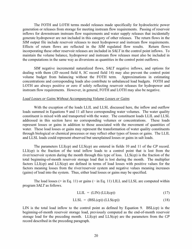
loads summed in Equations 9 and 11 all have corresponding water volumes. The water quality constituent is mixed with and transported with the water. The constituent loads LLIL and LLSL addressed in this section have no corresponding volumes or concentrations. These loads represent losses or gains in addition to those associated with the movement of quantities of water. These load losses or gains may represent the transformation of water quality constituents through biological or chemical processes or may reflect other types of losses or gains. The LLIL and LLSL loads could represent observed but unexplained losses or gains in salt loads.

The parameters LLI(cp) and LLS(cp) are entered in fields 10 and 11 of the CP record.

LLI(cp) is the fraction of the total inflow loads to a control point that is lost from the river/reservoir system during the month through this type of loss. LLS(cp) is the fraction of the total beginning-of-month reservoir storage load that is lost during the month. The multiplier factors LLI(cp) and LLS(cp) are defined in terms of load losses with positive values for the factors meaning losses from the river/reservoir system and negative values meaning increases (gains) of load into the system. Thus, either load losses or gains may be specified.

The load losses (+ in Eq. 11) or gains (− in Eq. 11) LILL and LLSL are computed within

program SALT as follows.

LLIL = (LIN) (LLI(cp)) (17)

LLSL = (BSL(cp)) (LLS(cp)) (18) LIN is the total load inflow to the control point as defined by Equation 9. BSL(cp) is the beginning-of-month reservoir storage load, previously computed as the end-of-month reservoir storage load for the preceding month. LLI(cp) and LLS(cp) are the parameters from the CP record described in the preceding paragraph.

21

Outflow from Control Points with No Reservoir Storage

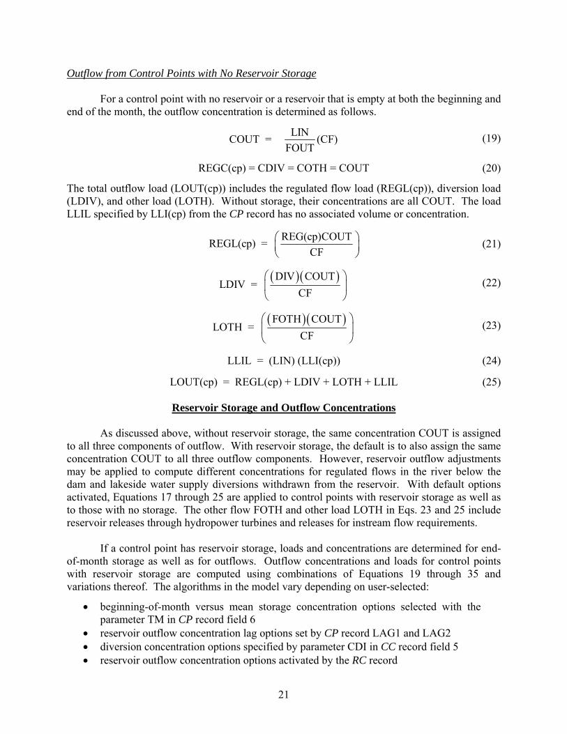
For a control point with no reservoir or a reservoir that is empty at both the beginning and end of the month, the outflow concentration is determined as follows.

LINCOUT = (CF)FOUT

(19)

REGC(cp) = CDIV = COTH = COUT (20)

The total outflow load (LOUT(cp)) includes the regulated flow load (REGL(cp)), diversion load (LDIV), and other load (LOTH). Without storage, their concentrations are all COUT. The load LLIL specified by LLI(cp) from the CP record has no associated volume or concentration. REG(cp)COUTREGL(cp) =

CF⎛ ⎞⎜ ⎟⎝ ⎠

(21)

( )( )DIV COUTLDIV =

CF⎛ ⎞⎜ ⎟⎝ ⎠

(22)

( )( )FOTH COUTLOTH =

CF⎛ ⎞⎜ ⎟⎝ ⎠

(23)

LLIL = (LIN) (LLI(cp)) (24)

LOUT(cp) = REGL(cp) + LDIV + LOTH + LLIL (25)

Reservoir Storage and Outflow Concentrations As discussed above, without reservoir storage, the same concentration COUT is assigned to all three components of outflow. With reservoir storage, the default is to also assign the same concentration COUT to all three outflow components. However, reservoir outflow adjustments may be applied to compute different concentrations for regulated flows in the river below the dam and lakeside water supply diversions withdrawn from the reservoir. With default options activated, Equations 17 through 25 are applied to control points with reservoir storage as well as to those with no storage. The other flow FOTH and other load LOTH in Eqs. 23 and 25 include reservoir releases through hydropower turbines and releases for instream flow requirements.

If a control point has reservoir storage, loads and concentrations are determined for end-of-month storage as well as for outflows. Outflow concentrations and loads for control points with reservoir storage are computed using combinations of Equations 19 through 35 and variations thereof. The algorithms in the model vary depending on user-selected:

• beginning-of-month versus mean storage concentration options selected with the parameter TM in CP record field 6

• reservoir outflow concentration lag options set by CP record LAG1 and LAG2 • diversion concentration options specified by parameter CDI in CC record field 5 • reservoir outflow concentration options activated by the RC record

22

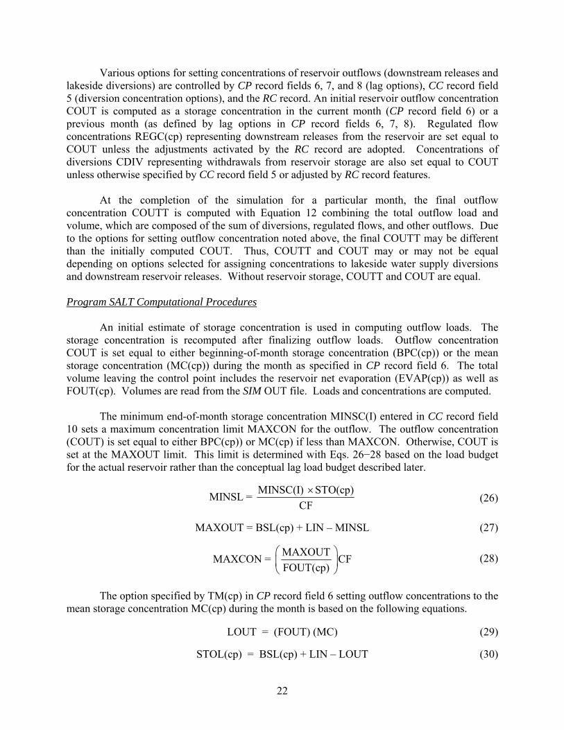
Various options for setting concentrations of reservoir outflows (downstream releases and lakeside diversions) are controlled by CP record fields 6, 7, and 8 (lag options), CC record field 5 (diversion concentration options), and the RC record. An initial reservoir outflow concentration COUT is computed as a storage concentration in the current month (CP record field 6) or a previous month (as defined by lag options in CP record fields 6, 7, 8). Regulated flow concentrations REGC(cp) representing downstream releases from the reservoir are set equal to COUT unless the adjustments activated by the RC record are adopted. Concentrations of diversions CDIV representing withdrawals from reservoir storage are also set equal to COUT unless otherwise specified by CC record field 5 or adjusted by RC record features.

At the completion of the simulation for a particular month, the final outflow

concentration COUTT is computed with Equation 12 combining the total outflow load and volume, which are composed of the sum of diversions, regulated flows, and other outflows. Due to the options for setting outflow concentration noted above, the final COUTT may be different than the initially computed COUT. Thus, COUTT and COUT may or may not be equal depending on options selected for assigning concentrations to lakeside water supply diversions and downstream reservoir releases. Without reservoir storage, COUTT and COUT are equal. Program SALT Computational Procedures

An initial estimate of storage concentration is used in computing outflow loads. The storage concentration is recomputed after finalizing outflow loads. Outflow concentration COUT is set equal to either beginning-of-month storage concentration (BPC(cp)) or the mean storage concentration (MC(cp)) during the month as specified in CP record field 6. The total volume leaving the control point includes the reservoir net evaporation (EVAP(cp)) as well as FOUT(cp). Volumes are read from the SIM OUT file. Loads and concentrations are computed.

The minimum end-of-month storage concentration MINSC(I) entered in CC record field

10 sets a maximum concentration limit MAXCON for the outflow. The outflow concentration (COUT) is set equal to either BPC(cp)) or MC(cp) if less than MAXCON. Otherwise, COUT is set at the MAXOUT limit. This limit is determined with Eqs. 26−28 based on the load budget for the actual reservoir rather than the conceptual lag load budget described later.

MINSC(I) STO(cp)MINSL =

CF×

(26)

MAXOUT = BSL(cp) + LIN – MINSL (27) MAXOUTMAXCON = CF

FOUT(cp)⎛ ⎞⎜ ⎟⎝ ⎠

(28)

The option specified by TM(cp) in CP record field 6 setting outflow concentrations to the

mean storage concentration MC(cp) during the month is based on the following equations. LOUT = (FOUT) (MC) (29) STOL(cp) = BSL(cp) + LIN – LOUT (30)

23

BSL(cp) + STOL(cp)MC = CFBSTO(cp) + STO(cp)

⎛ ⎞⎜ ⎟⎝ ⎠

(31)

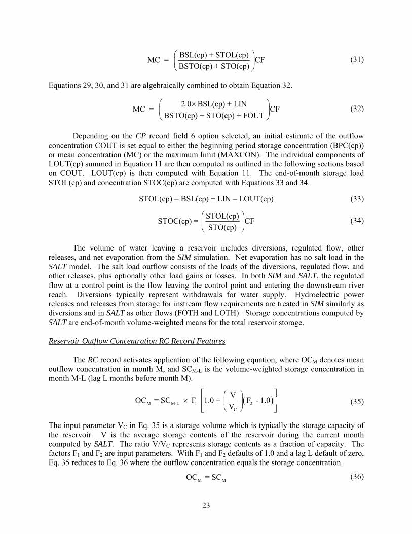
Equations 29, 30, and 31 are algebraically combined to obtain Equation 32. 2.0 BSL(cp) + LINMC = CF

BSTO(cp) + STO(cp) + FOUT⎛ ⎞×⎜ ⎟⎝ ⎠

(32)

Depending on the CP record field 6 option selected, an initial estimate of the outflow concentration COUT is set equal to either the beginning period storage concentration (BPC(cp)) or mean concentration (MC) or the maximum limit (MAXCON). The individual components of LOUT(cp) summed in Equation 11 are then computed as outlined in the following sections based on COUT. LOUT(cp) is then computed with Equation 11. The end-of-month storage load STOL(cp) and concentration STOC(cp) are computed with Equations 33 and 34. STOL(cp) = BSL(cp) + LIN – LOUT(cp) (33) STOL(cp)STOC(cp) = CF

STO(cp)⎛ ⎞⎜ ⎟⎝ ⎠

(34)

The volume of water leaving a reservoir includes diversions, regulated flow, other

releases, and net evaporation from the SIM simulation. Net evaporation has no salt load in the SALT model. The salt load outflow consists of the loads of the diversions, regulated flow, and other releases, plus optionally other load gains or losses. In both SIM and SALT, the regulated flow at a control point is the flow leaving the control point and entering the downstream river reach. Diversions typically represent withdrawals for water supply. Hydroelectric power releases and releases from storage for instream flow requirements are treated in SIM similarly as diversions and in SALT as other flows (FOTH and LOTH). Storage concentrations computed by SALT are end-of-month volume-weighted means for the total reservoir storage.

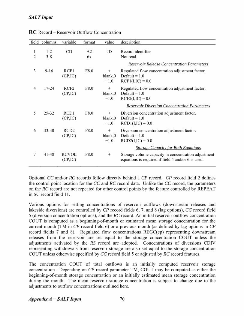
Reservoir Outflow Concentration RC Record Features The RC record activates application of the following equation, where OCM denotes mean outflow concentration in month M, and SCM-L is the volume-weighted storage concentration in month M-L (lag L months before month M).

( )M M-L 1 2

C

VOC = SC F 1.0 + F - 1.0V

⎡ ⎤⎛ ⎞× ⎢ ⎥⎜ ⎟

⎝ ⎠⎣ ⎦ (35)

The input parameter VC in Eq. 35 is a storage volume which is typically the storage capacity of the reservoir. V is the average storage contents of the reservoir during the current month computed by SALT. The ratio V/VC represents storage contents as a fraction of capacity. The factors F1 and F2 are input parameters. With F1 and F2 defaults of 1.0 and a lag L default of zero, Eq. 35 reduces to Eq. 36 where the outflow concentration equals the storage concentration.

M MOC = SC (36)

24

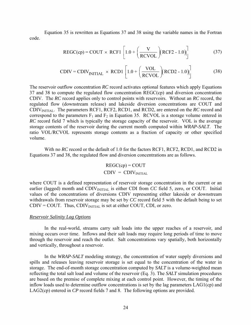
Equation 35 is rewritten as Equations 37 and 38 using the variable names in the Fortran code.

( )VREGC(cp) = COUT RCF1 1.0 + RCF2 - 1.0RCVOL

⎡ ⎤⎛ ⎞× ⎜ ⎟⎢ ⎥⎝ ⎠⎣ ⎦

(37)

( )INITIALVOLCDIV = CDIV RCD1 1.0 + RCD2 - 1.0

RCVOL⎡ ⎤⎛ ⎞× ⎜ ⎟⎢ ⎥⎝ ⎠⎣ ⎦

(38)

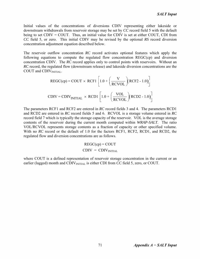
The reservoir outflow concentration RC record activates optional features which apply Equations 37 and 38 to compute the regulated flow concentration REGC(cp) and diversion concentration CDIV. The RC record applies only to control points with reservoirs. Without an RC record, the regulated flow (downstream release) and lakeside diversion concentrations are COUT and CDIVINITIAL. The parameters RCF1, RCF2, RCD1, and RCD2, are entered on the RC record and correspond to the parameters F1 and F2 in Equation 35. RCVOL is a storage volume entered in RC record field 7 which is typically the storage capacity of the reservoir. VOL is the average storage contents of the reservoir during the current month computed within WRAP-SALT. The ratio VOL/RCVOL represents storage contents as a fraction of capacity or other specified volume. With no RC record or the default of 1.0 for the factors RCF1, RCF2, RCD1, and RCD2 in Equations 37 and 38, the regulated flow and diversion concentrations are as follows.

REGC(cp) = COUT

CDIV = CDIVINITIAL where COUT is a defined representation of reservoir storage concentration in the current or an earlier (lagged) month and CDIVINITIAL is either CDI from CC field 5, zero, or COUT. Initial values of the concentrations of diversions CDIV representing either lakeside or downstream withdrawals from reservoir storage may be set by CC record field 5 with the default being to set CDIV = COUT. Thus, CDIVINITIAL is set at either COUT, CDI, or zero. Reservoir Salinity Lag Options In the real-world, streams carry salt loads into the upper reaches of a reservoir, and mixing occurs over time. Inflows and their salt loads may require long periods of time to move through the reservoir and reach the outlet. Salt concentrations vary spatially, both horizontally and vertically, throughout a reservoir. In the WRAP-SALT modeling strategy, the concentration of water supply diversions and spills and releases leaving reservoir storage is set equal to the concentration of the water in storage. The end-of-month storage concentration computed by SALT is a volume-weighted mean reflecting the total salt load and volume of the reservoir (Eq. 3). The SALT simulation procedures are based on the premise of complete mixing at each control point. However, the timing of the inflow loads used to determine outflow concentrations is set by the lag parameters LAG1(cp) and LAG2(cp) entered in CP record fields 7 and 8. The following options are provided.

25

• If CP record fields 7 and 8 are left blank, the lag features are not activated for that control point. The simulation is based on complete mixing within each month.

• The lag options based on the variable LAG are controlled by LAG1(cp) and

LAG2(cp) entered in CP record fields 7 and 8. A non-zero LAG1(cp) activates use of the lag features. LAG2(cp) selects the manner in which LAG is determined.

1. With no entry for LAG2(cp) in CP field 8, the option is activated in

which LAG is set equal to LAG1(cp) from field 7. Thus, the model-user sets a constant LAG that is applied during every month of the simulation.

2. With an entry for LAG2(cp) in CP field 8, a variable LAG is computed in

each month based on the concept of retention time. LAG2(cp) is a multiplier factor used in the computation of the retention time parameter.

A non-zero LAG1(cp) entered in CP record field 7 is required for either lag option. LAG1(cp) is an integer number of months. For the first lag option, LAG1(cp) is a constant lag adopted in every month. LAG1(cp) serves as the only activation parameter for the first option. A non-zero LAG2(cp) entered in CP record field 8 activates the second option. For the second option, LAG1(cp) is the upper limit on lag computed each month based on the concept of retention time. LAG2(cp) is a multiplier factor in the form of a decimal (real) number. The lag options are based on the premise that salt entering the reservoir in a particular month begins to reach the outlet LAG months later. Complete mixing occurs during the LAG months. Thus, the salt leaves the reservoir over a period of multiple months that begins LAG months after the month in which the quantity of salt entered the reservoir.

Salt load budgets result in end-of-month reservoir load for each month based on an accounting balance of inflow and outflow loads combined with the end-of-month storage load from the preceding month. With the lag features activated, two load budgets are maintained. The regular load budget maintained with or without the lag features reflect the actual total loads in storage with the corresponding volume-weighted mean storage concentrations. The second conceptual computational load budget based on lagged load inflows is maintained solely for the purpose of determining the outflow concentration each month. The timing of the load inflow to this computational load-budget reservoir is controlled by the LAG. With the exception of the timing of the salt load inflows, the salinity simulation algorithms are applied in essentially the same manner for maintaining the salt load budgets both with and without the LAG.

The lag options are pertinent only for control points with significant reservoir storage.

Without storage, complete mixing during the month without lag is assumed in the model. Selection of the CP record reservoir lag parameters LAG1(cp) and LAG2(cp) are necessarily judgmental and may be somewhat arbitrary. They may be treated as calibration parameters in situations where observed data are available for calibration. Lag determined by calibration for reservoirs with observed data may be relevant to other reservoirs as well. Sensitivity analyses with alternative simulations with varying values for the lag parameters may be made to investigate their effects on simulation results.

26

Computation of LAG Based on Retention Time With a non-zero LAG2(cp), the variable LAG in months is computed based on retention time as outlined below. LAG1(cp) is a maximum upper limit on LAG. LAG2(cp) is a multiplier factor that is incorporated in the computation of the retention time parameter. Retention time is a representation of the time required for a monthly volume of water and its salt load to flow through a reservoir. Retention time is defined as follows. reservoir storage volumeretention time in months =

outflow volume per month

(39)

The computation of LAG is based on computing the parameter ZLAG for each

cumulative set of L months from a L of 1 month to a L of MAXL=LAG1(cp) months, where L represents a time period extending backward from the current month. ( )BSTO(cp) + Σ BSTO(cp,L) / (L+1)

ZLAG = LAG2(cp)Σ FOUT(cp,L)/L

⎛ ⎞⎜ ⎟⎝ ⎠

(40)

BSTO(cp) is the beginning-of-month storage for the current month. ∑BSTO(cp,L) and ∑FOUT(cp,L) are the summations for the preceding L months of the beginning-of-month storage and the outflow during the month. LAG2(cp) is a parameter from CP record field 8 that may be set at 1.0 if calibration or other information is not available to suggest another value. ZLAG is first computed for the month preceding the current month. Based on the results, either LAG is set or ZLAG is determined for a longer period of time.

If ZLAG < 1.0 then LAG = 0

If 1.0 ≤ ZLAG < 2.0 then LAG = 1 month If ZLAG for one month is 2.0 or more, a second ZLAG is computed for the two month period preceding the current month.

If ZLAG < 3.0 then LAG = 2 months Otherwise, ZLAG is computed for the three month period preceding the current month.

If ZLAG < 4.0 then LAG = 3 months The procedure continues until the length of the preceding period reaches the maximum limit of LAG1(cp) months from the CP record. LAG is set equal to LAG1(cp) if this limit is reached. Incorporation of LAG in the Load Budget Simulation LAG may be treated as a monthly varying variable set based on retention time as outlined above. Alternatively, LAG may be a constant set by the model-user. LAG is applied in a similar manner regardless of the option adopted for its determination.

27

A separate load budget for a conceptual computational reservoir is maintained for the sole purpose of computing the outflow concentration for the current month. The load inflow (ZLIN) for this load-budget for the current month is the actual load inflow (LIN) for the month that is LAG months earlier plus the inflow loads for any other months prior to LAG months ago that have not yet been activated. If LAG extends back to before the first month of the simulation, the load budget is based on setting the outflow concentrations equal to the reservoir storage concentration at the beginning of the current month and inflow load equal to outflow load. Salinity Example 1 - Simplified Example of Routing a Slug of Salt through a Reservoir The lag represents physically the time required for salt entering the reservoir during a month to reach the outlet. The salt is assumed to be completely mixed during the lag time. The load entering a reservoir in a particular month leaves the reservoir over multiple months beginning LAG months after entering. The following hypothetical example illustrates the computational strategy by focusing on the salt load entering a reservoir in a single month. Several months are required for the slug of salt to pass through the reservoir. A constant inflow volume of 10,000 acre-feet/month and outflow of 10,000 acre-feet/month occur in every month of the simulation. The reservoir storage volume remains at a constant 50,000 ac-ft. The net evaporation-precipitation is zero. These quantities are provided by the SIM output file and of course typically unlike this example will vary monthly. In month 1, the inflow has a concentration of 1,000 mg/l and load of: FIN (CIN) (10,000 ac-ft)(1,000 mg/l)LIN = = = 13,597 tons

CF 735.48

The inflow load of 13,597 tons in month 1 is the only salt entering the reservoir. The inflow concentration is zero in all other months of the simulation. The storage concentration is zero at the beginning of the simulation. Thus, this simplified hypothetical example is designed to demonstrate how the salt load in a particular month moves through the reservoir according to the model. Of course, in actual applications, salt inflow loads will be non-zero in every month. The parameters entered on the CP record for this example are as follows.

CP record field 6: Default results in use of mean concentration based on Eq. 32.

CP record field 7: Any integer greater than 5 for LAG1(cp) yields the same results.

CP record field 8: LAG2(cp) of 1.0. The lag (LAG) computed by the repetitive algorithm based on Eq. 40 is 5 months. Beginning with L = 1 month, ZLAG = 5.0 which is greater than 2 months. ( )50,000 + 50,000 / (1+1)

ZLAG = (1.0) = 5.0 10,000 / 1

⎛ ⎞⎜ ⎟⎝ ⎠

28

Table 3 Simulation Results for Example 1

Computation of Outflow Concentration Inflow Storage Storage Inflow Storage Storage Outflow Outflow

Month Load Load Conc Load Load Conc Conc Load (tons) (tons) (mg/l) (tons) (tons) (mg/l) (mg/l) (tons)

1 2 3 4 5 6 7 8 9

0 0 0 1 13,597 0 0 0 0 13,597 200 0

2 0 0 0 0 0 13,597 200 0

3 0 0 0 0 0 13,597 200 0

4 0 0 0 0 0 13,597 200 0

5 0 0 0 0 0 13,597 200 0

6 0 13,597 90.9 90.9 1,236 12,361 181.8 12,361

7 0 0 165.3 165.3 2,247 10,113 148.8 10,113

8 0 0 135.2 135.2 1,839 8,274 121.7 8,274

9 0 0 110.6 110.6 1,504 6,770 99.6 6,770

10 0 0 90.5 90.5 1,231 5,539 81.5 5,539

11 0 0 74.1 74.1 1,007 4,532 66.7 4,532

12 0 0 60.6 60.6 824 3,708 54.5 3,708

13 0 0 49.6 49.6 674 3,034 44.6 3,034

14 0 0 40.6 40.6 552 2,483 36.5 2,483

15 0 0 33.2 33.2 451 2,031 29.9 2,031

16 0 0 27.2 27.2 369 1,662 24.4 1,662

17 0 0 22.2 22.2 302 1,360 20.0 1,360

18 0 0 18.2 18.2 247 1,113 16.4 1,113

---------------------------------------------------------------------------------------- 37.3 0.55 37.3

36 0 0 0.49 0.49 6.67 30.6 0.45 30.6

29

After four more repetitions, L = 5 which is less than 6.0 and thus LAG = 5 months. ( )50,000 + 200,000 / (5+1)

ZLAG = (1.0) = 5.0 50,000 / 5

⎛ ⎞⎜ ⎟⎝ ⎠

With constant inflow volume, outflow volume, and storage volume, the retention time of 5 months and the LAG of 5 months are the same for every month of the simulation.

Simulation results are presented in Table 3. With no salt in the reservoir at the beginning and an inflow of 13,597 tons during month 1, the salt load at the end of month 1 is 13,597 tons, and the storage concentration is:

STOL(cp) 13,597 tonsSTOC(cp) = CF = 735.48 200 mg/lSTO(cp) 50,000 ac-ft

⎛ ⎞ ⎛ ⎞ =⎜ ⎟ ⎜ ⎟⎝ ⎠⎝ ⎠

The end-of-month storage load and volume-weighted mean end-of-month storage concentration are tabulated in columns 3 and 4 of Table 3. The lagged load budget used to determine the outflow concentration is tabulated in columns 5 through 8. The mean storage and outflow concentration (COUT = MC) computed with Eq. 32 is tabulated in columns 8 and 9. The outflow load (Eq. 30) is shown in column 9. With a LAG of 5 months, the 13,597 tons of salt entering the reservoir in month 1 begins to affect the outflow concentration in month 6. The actual end-of-month storage load (column 2) decreases from 13,597 tons in month 5 to 1,112 tons in month 18, to 30 tons in month 36, and 2.7 tons in month 48. Salinity Example 2 – Effects of Lag Options Example 2 is designed to further illustrate the reservoir salinity inflow lag options. The input data files are included in the set of electronic input files for all of the WRAP examples and can be used to experiment with SALT. The example is comprised of simple unrealistic data designed to allow the simulation computations to be easily tracked. The SIM input DAT file and SALT input SIN file are reproduced as Tables 4 and 5. The variables in each field of the DAT file are defined in the Users Manual. The records in the SIN file are explained in Appendix A.

Example 2 has one control point, one reservoir, and a 3-year hydrologic period-of-analysis. The loads and concentrations could be for total dissolved solids or any other conservative water quality constituent. The DAT and SIN files reproduced as Tables 4 and 5 contain the complete input dataset for this example. WRAP-SIM is executed with the DAT file to obtain a SIM simulation results output OUT file, which is not shown. WRAP-SALT reads the OUT and SIN files and produces the optional SMS file tables shown as Tables 6 and 7. In most actual modeling applications, a SAL file will be produced with SALT to be read by program TABLES to create a set of tables organizing the salinity simulation results. However, TABLES is not applied in this simple hypothetical example. The tables normally produced with TABLES are illustrated later by the much larger and more realistic example at the end of this chapter.

30

Two alternative lag options are compared. Two simulations are presented with the only input data difference being the lag option selected on the CP record. Both alternative CP records are included in the SIN file shown in Table 5, with one of the CP records deactivated with ** entered as the first two characters of the record. LAG2(cp) is zero (blank CP record field 8) and 1.0 for the two alternative simulations. LAG1(cp) is six months in both simulations. Simulation results tables from the SALT output SMS file for the two alternative simulations are reproduced as Tables 6 and 7. The first SMS file table shown in Tables 6 and 7 is a tabulation of monthly simulation results in a format designed for tracking the reservoir lag computations. The second table is a volume and load summary. The SALT message SMS file table at the top of Tables 6 and 7 is designed specifically to facilitate tracking of the lag computations. Model-users can experiment with this simplified example to gain insight to the lag computations. The total volume and load budget summary reproduced at the bottom of Tables 6 and 7 is designed for routine viewing with essentially any SALT simulation application. These and other SALT output tables found in the SMS and SAL files are discussed later in this chapter. This dataset is purposely designed for illustrative purposes to have the same load inflow in each of the 36 months of the simulation. The combination of stream flow volumes on the IN records in the DAT file (Table 4) and salt concentrations on the S1 records in the SIN file (Table 5) result in the same load of 10,000 tons/month in each month of the three year 2001-2002 period-of-analysis.

The SALT simulation results shown in Table 6 reflect a constant lag of 6 months entered on the CP record for control point CP-1. LAG2(cp) is zero (blank CP record field 8). The constant lag option serves solely to lag the inflow loads. However, since the load inflows are a constant 10,000 tons/month in every month in this example, the SALT simulation results are identical with no lag or a lag of 1 month, 6 months, or any other integer number of months. The only difference between the input data for the two alternative simulations is the entry for LAG2(cp) on the CP record in the SIN file. For the second simulation, the CP record is altered to set LAG2(cp) at 1.0 which activates the variable lag option. The LAG1(cp) of 6 months from the CP record is now an upper limit on the computed lag. The SALT simulation results are shown in Table 7.

The lag computed in each month is tabulated in the fourth column of Table 7. The actual inflow load LIN each month is in the fifth column. The inflow load ZLIN flowing into the computational lag reservoir is shown in the sixth column. The maximum lag limit of 6 months is adopted by the SALT simulation computations from January through November 2001 based on iteratively applying Equation 40. The retention time computations result in a lag of 4 months in December 2001. In order to properly maintain a balance load budget, the variable lag option algorithm must ensure that all reservoir inflow loads are included in the computations as the lag changes. ZLIN is 30,000 tons to cover the two preceding months as well as the lag 4 month. Thus, the lag reservoir inflow loads change with changes in the computed lag. Similarly, ZLIN is zero in March 2002 when the lag reduces from four months to three months.

31

A reservoir outflow concentration RC record is included in the SIN file shown in Table 5 for illustrative purposes. The parameters RCF1, RCF2, RCD1, and RCD2 are all set at 1.0. As previously discussed, with the parameters all set at their default of 1.0, the RC record has no effect on the simulation results. However, if RCF1, RCF2, RCD1, and RCD2 are set at values other than 1.0, Equations 37 and 38 are incorporated into the computation of regulated flow concentrations and diversion concentrations. Flow volumes on the IN records in the DAT file are in units of acre-feet/month. Concentrations on the CC and S1 records in the SIN file are in tons/acre-foot. With a conversion factor CF of 1.0 entered in SC record field 15, loads are in units of tons/month.

Table 4 SIM DAT File for Salinity Example 2

T1 WRAP-SIM Input File SaltExam2.DAT T2 Salinity Manual Example 2 - Effects of Lag Options T3 May 2009 ** 1 2 3 4 5 **345678901234567890123456789012345678901234567890123456 JD 3 2001 1 -1 JO 3 CP CP-1 OUT 0 NONE WR CP-1 WS ResA 6000. 1.0 1.0 ED ** Naturalized flows in acre-feet IN CP-1 2001 1000. 1000. 1000. 1000. 1000. 1000. 500. 500. 500. 2000. 2000. 2000. IN CP-1 2002 1000. 1000. 1000. 1000. 1000. 1000. 500. 500. 500. 2000. 2000. 2000. IN CP-1 2003 1000. 1000. 1000. 1000. 1000. 1000. 1000. 1000. 1000. 1000. 1000. 1000.

Table 5 SALT SIN File for Salinity Example 2

** WRAP-SALT Input File SaltExam2.SIN ** Salinity Manual Example 2 - Effects of Lag Options ** May 2009 ** 1 2 3 4 5 6 7 8 9 10 11 **34567890123456789012345678901234567890123456789012345678901234567890123456789012345678901234567890123456789012 ** ! ! ! ! ! ! ! ! ! ! ! ! ! ! ! ! ! ! ! ! SC 2001 3 0 0 0 2 2 0 0 0 2 4 0 1.0 ** ** The only difference in the two variations of the CP record is the LAG2 of zero (blank) versus 1.0. CP CP-1 6 6000. **CP CP-1 6 1.0 6000. CC 10. ** The RC record has no effect on simulation results with the four factors all set equal to the default of 1.0. RC 1.0 1.0 1.0 1.0 6000. ED ** Concentrations in tons/acre-foot S1 CP-1 2001 10.0 10.0 10.0 10.0 10.0 10.0 20.0 20.0 20.0 5.0 5.0 5.0 S1 CP-1 2002 10.0 10.0 10.0 10.0 10.0 10.0 20.0 20.0 20.0 5.0 5.0 5.0 S1 CP-1 2002 10.0 10.0 10.0 10.0 10.0 10.0 10.0 10.0 10.0 10.0 10.0 10.0

32

Table 6 SALT Output SMS File Tables for Constant Lag of 6 Months

YEAR M CPID LAG LIN ZLIN STOL STOLLAG STO FOUT LOUT STOC STOCLAG COUT 2001 1 CP-1 6 10000.0 10000.0 60000.0 60000.0 6000.0 1000.0 10000.0 10.0 10.0 10.0 2001 2 CP-1 6 10000.0 10000.0 60000.0 60000.0 6000.0 1000.0 10000.0 10.0 10.0 10.0 2001 3 CP-1 6 10000.0 10000.0 60000.0 60000.0 6000.0 1000.0 10000.0 10.0 10.0 10.0 2001 4 CP-1 6 10000.0 10000.0 60000.0 60000.0 6000.0 1000.0 10000.0 10.0 10.0 10.0 2001 5 CP-1 6 10000.0 10000.0 60000.0 60000.0 6000.0 1000.0 10000.0 10.0 10.0 10.0 2001 6 CP-1 6 10000.0 10000.0 60000.0 60000.0 6000.0 1000.0 10000.0 10.0 10.0 10.0 2001 7 CP-1 6 10000.0 10000.0 64800.0 64800.0 6000.0 500.0 5200.0 10.8 10.8 10.4 2001 8 CP-1 6 10000.0 10000.0 69216.0 69216.0 6000.0 500.0 5584.0 11.5 11.5 11.2 2001 9 CP-1 6 10000.0 10000.0 73278.7 73278.7 6000.0 500.0 5937.3 12.2 12.2 11.9 2001 10 CP-1 6 10000.0 10000.0 60913.4 60913.4 6000.0 2000.0 22365.3 10.2 10.2 11.2 2001 11 CP-1 6 10000.0 10000.0 52081.0 52081.0 6000.0 2000.0 18832.4 8.7 8.7 9.4 2001 12 CP-1 6 10000.0 10000.0 45772.1 45772.1 6000.0 2000.0 16308.9 7.6 7.6 8.2 2002 1 CP-1 6 10000.0 10000.0 47961.0 47961.0 6000.0 1000.0 7811.1 8.0 8.0 7.8 2002 2 CP-1 6 10000.0 10000.0 49813.2 49813.2 6000.0 1000.0 8147.9 8.3 8.3 8.1 2002 3 CP-1 6 10000.0 10000.0 51380.4 51380.4 6000.0 1000.0 8432.8 8.6 8.6 8.4 2002 4 CP-1 6 10000.0 10000.0 52706.5 52706.5 6000.0 1000.0 8673.9 8.8 8.8 8.7 2002 5 CP-1 6 10000.0 10000.0 53828.6 53828.6 6000.0 1000.0 8877.9 9.0 9.0 8.9 2002 6 CP-1 6 10000.0 10000.0 54778.0 54778.0 6000.0 1000.0 9050.5 9.1 9.1 9.1 2002 7 CP-1 6 10000.0 10000.0 59995.8 59995.8 6000.0 500.0 4782.2 10.0 10.0 9.6 2002 8 CP-1 6 10000.0 10000.0 64796.1 64796.1 6000.0 500.0 5199.7 10.8 10.8 10.4 2002 9 CP-1 6 10000.0 10000.0 69212.4 69212.4 6000.0 500.0 5583.7 11.5 11.5 11.2 2002 10 CP-1 6 10000.0 10000.0 58008.9 58008.9 6000.0 2000.0 21203.5 9.7 9.7 10.6 2002 11 CP-1 6 10000.0 10000.0 50006.3 50006.3 6000.0 2000.0 18002.5 8.3 8.3 9.0 2002 12 CP-1 6 10000.0 10000.0 44290.2 44290.2 6000.0 2000.0 15716.1 7.4 7.4 7.9 2003 1 CP-1 6 10000.0 10000.0 46707.1 46707.1 6000.0 1000.0 7583.1 7.8 7.8 7.6 2003 2 CP-1 6 10000.0 10000.0 48752.2 48752.2 6000.0 1000.0 7954.9 8.1 8.1 8.0 2003 3 CP-1 6 10000.0 10000.0 50482.6 50482.6 6000.0 1000.0 8269.6 8.4 8.4 8.3 2003 4 CP-1 6 10000.0 10000.0 51946.8 51946.8 6000.0 1000.0 8535.8 8.7 8.7 8.5 2003 5 CP-1 6 10000.0 10000.0 53185.8 53185.8 6000.0 1000.0 8761.1 8.9 8.9 8.8 2003 6 CP-1 6 10000.0 10000.0 54234.1 54234.1 6000.0 1000.0 8951.7 9.0 9.0 9.0 2003 7 CP-1 6 10000.0 10000.0 55121.2 55121.2 6000.0 1000.0 9112.9 9.2 9.2 9.1 2003 8 CP-1 6 10000.0 10000.0 55871.8 55871.8 6000.0 1000.0 9249.4 9.3 9.3 9.2 2003 9 CP-1 6 10000.0 10000.0 56506.9 56506.9 6000.0 1000.0 9364.9 9.4 9.4 9.4 2003 10 CP-1 6 10000.0 10000.0 57044.3 57044.3 6000.0 1000.0 9462.6 9.5 9.5 9.5 2003 11 CP-1 6 10000.0 10000.0 57499.0 57499.0 6000.0 1000.0 9545.3 9.6 9.6 9.5 2003 12 CP-1 6 10000.0 10000.0 57883.8 57883.8 6000.0 1000.0 9615.2 9.6 9.6 9.6 Total Volume and Load Summary for Constituent 1

Volume Load Concentration

Naturalized flows 39000. 360000. 9.2 Regulated flows at boundary 0. 0. 0.0 Return flows 0. 0. 0.0 CI record constant inflows 0. 0. 0.0 Channel loss credits 0. 0. 0.0 Channel losses 0. 0. 0.0 Regulated flows at outlet 39000. 362116. 9.3 Diversions 0. 0. 0.0 Other flows and loads 0. 0. 0.0 Net evaporation 0. 0. 0.0 ---------- ---------- ---------- Inflows - Outflows 0. -2116. 0.0 ---------- ---------- ---------- Beginning reservoir storage 6000. 60000. 10.0 Ending reservoir storage 6000. 57884. 9.6 ---------- ---------- ---------- Change in storage 0. -2116. 0.0 ---------- ---------- ---------- Volume and load differences 0. 0. 0.0

Naturalized flows at outlet 39000.

33

Table 7 SALT Output SMS File Tables for Variable Lag

YEAR M CPID LAG LIN ZLIN STOL STOLLAG STO FOUT LOUT STOC STOCLAG COUT 2001 1 CP-1 6 10000.0 10000.0 60000.0 60000.0 6000.0 1000.0 10000.0 10.0 10.0 10.0 2001 2 CP-1 6 10000.0 10000.0 60000.0 60000.0 6000.0 1000.0 10000.0 10.0 10.0 10.0 2001 3 CP-1 6 10000.0 10000.0 60000.0 60000.0 6000.0 1000.0 10000.0 10.0 10.0 10.0 2001 4 CP-1 6 10000.0 10000.0 60000.0 60000.0 6000.0 1000.0 10000.0 10.0 10.0 10.0 2001 5 CP-1 6 10000.0 10000.0 60000.0 60000.0 6000.0 1000.0 10000.0 10.0 10.0 10.0 2001 6 CP-1 6 10000.0 10000.0 60000.0 60000.0 6000.0 1000.0 10000.0 10.0 10.0 10.0 2001 7 CP-1 6 10000.0 10000.0 64800.0 64800.0 6000.0 500.0 5200.0 10.8 10.8 10.4 2001 8 CP-1 6 10000.0 10000.0 69216.0 69216.0 6000.0 500.0 5584.0 11.5 11.5 11.2 2001 9 CP-1 6 10000.0 10000.0 73278.7 73278.7 6000.0 500.0 5937.3 12.2 12.2 11.9 2001 10 CP-1 6 10000.0 10000.0 60913.4 60913.4 6000.0 2000.0 22365.3 10.2 10.2 11.2 2001 11 CP-1 6 10000.0 10000.0 52081.0 52081.0 6000.0 2000.0 18832.4 8.7 8.7 9.4 2001 12 CP-1 4 10000.0 30000.0 42915.0 62915.0 6000.0 2000.0 19166.0 7.2 10.5 9.6 2002 1 CP-1 3 10000.0 20000.0 41697.3 71697.3 6000.0 1000.0 11217.7 6.9 11.9 11.2 2002 2 CP-1 3 10000.0 10000.0 39897.7 69897.7 6000.0 1000.0 11799.6 6.6 11.6 11.8 2002 3 CP-1 4 10000.0 0.0 39144.2 59144.2 6000.0 1000.0 10753.5 6.5 9.9 10.8 2002 4 CP-1 4 10000.0 10000.0 39275.9 59275.9 6000.0 1000.0 9868.3 6.5 9.9 9.9 2002 5 CP-1 5 10000.0 0.0 40156.5 50156.5 6000.0 1000.0 9119.4 6.7 8.4 9.1 2002 6 CP-1 6 10000.0 0.0 42440.1 42440.1 6000.0 1000.0 7716.4 7.1 7.1 7.7 2002 7 CP-1 6 10000.0 10000.0 48644.9 48644.9 6000.0 500.0 3795.2 8.1 8.1 7.6 2002 8 CP-1 6 10000.0 10000.0 54353.3 54353.3 6000.0 500.0 4291.6 9.1 9.1 8.6 2002 9 CP-1 6 10000.0 10000.0 59605.1 59605.1 6000.0 500.0 4748.3 9.9 9.9 9.5 2002 10 CP-1 6 10000.0 10000.0 51146.5 51146.5 6000.0 2000.0 18458.6 8.5 8.5 9.2 2002 11 CP-1 6 10000.0 10000.0 45104.6 45104.6 6000.0 2000.0 16041.8 7.5 7.5 8.0 2002 12 CP-1 4 10000.0 30000.0 37931.9 57931.9 6000.0 2000.0 17172.7 6.3 9.7 8.6 2003 1 CP-1 3 10000.0 20000.0 37480.8 67480.8 6000.0 1000.0 10451.1 6.2 11.2 10.5 2003 2 CP-1 3 10000.0 10000.0 36329.9 66329.9 6000.0 1000.0 11150.9 6.1 11.1 11.2 2003 3 CP-1 4 10000.0 0.0 36125.3 56125.3 6000.0 1000.0 10204.6 6.0 9.4 10.2 2003 4 CP-1 4 10000.0 10000.0 36721.4 56721.4 6000.0 1000.0 9403.9 6.1 9.5 9.4 2003 5 CP-1 5 10000.0 0.0 37995.0 47995.1 6000.0 1000.0 8726.4 6.3 8.0 8.7 2003 6 CP-1 6 10000.0 0.0 40611.2 40611.2 6000.0 1000.0 7383.9 6.8 6.8 7.4 2003 7 CP-1 6 10000.0 10000.0 43594.1 43594.1 6000.0 1000.0 7017.1 7.3 7.3 7.0 2003 8 CP-1 6 10000.0 10000.0 46118.1 46118.1 6000.0 1000.0 7476.0 7.7 7.7 7.5 2003 9 CP-1 6 10000.0 10000.0 48253.8 48253.8 6000.0 1000.0 7864.3 8.0 8.0 7.9 2003 10 CP-1 6 10000.0 10000.0 50060.9 50060.9 6000.0 1000.0 8192.9 8.3 8.3 8.2 2003 11 CP-1 6 10000.0 10000.0 51590.0 51590.0 6000.0 1000.0 8470.9 8.6 8.6 8.5 2003 12 CP-1 6 10000.0 10000.0 52883.8 52883.8 6000.0 1000.0 8706.1 8.8 8.8 8.7 Total Volume and Load Summary for Constituent 1 Volume Load Concentration Naturalized flows 39000. 360000. 9.2 Regulated flows at boundary 0. 0. 0.0 Return flows 0. 0. 0.0 CI record constant inflows 0. 0. 0.0 Channel loss credits 0. 0. 0.0 Channel losses 0. 0. 0.0 Regulated flows at outlet 39000. 367116. 9.4 Diversions 0. 0. 0.0 Other flows and loads 0. 0. 0.0 Net evaporation 0. 0. 0.0 ---------- ---------- ---------- Inflows - Outflows 0. -7116. 0.0 ---------- ---------- ---------- Beginning reservoir storage 6000. 60000. 10.0 Ending reservoir storage 6000. 52884. 8.8 ---------- ---------- ---------- Change in storage 0. -7116. 0.0 ---------- ---------- ---------- Volume and load differences 0. 0. 0.0 Naturalized flows at outlet 39000.

34

SALT Simulation Results The program SALT simulation results are written to two output files. The file with filename extension SAL is read by program TABLES. Additional information is provided in the message file, which has the filename extension SMS. The SMS file provides the following information, with options selected by SC record field 13 that may be useful in tracking the simulation and performing various analyses.

1. Trace messages track the simulation.

2. Error messages are written if errors or inconsistencies are detected in the input data. An error message is accompanied by termination of model execution.

3. Warning messages are activated by various situations that may occur during the

simulation. For example, warning messages are written if the minimum or maximum concentration limits specified in CC record fields 8, 9, 10, and 11 are reached. Irregularities in input data may generate a variety of warning messages.

4. A concise overall volume and load balance summary table is provided.

5. The components of detailed monthly control point volume and load balances are

recorded as computed in the simulation if specified by SC record field 13.

6. Reservoir lag results may be tabulated as illustrated by Tables 6 and 7.

7. An optional listing of control points with pertinent information may be written. The trace messages printed to the message (SMS) file during a successful execution of SALT are shown in Table 8. Some messages are printed only if certain options are activated, others are always found in the message file. The program contains routines that check the input data for blunders and inconsistencies. Numerous error and warning messages are possible. Program execution is terminated with an error message but continues with warning messages. The error and warning messages are inserted into the trace of Table 8 as problems are detected during model execution. The trace messages are designed primarily to track the reading of input data. The table discussed below tracks the simulation computations. An option activated by SC record field 13 allows essentially any and all of the quantities computed during the simulation to be recorded in the SMS file. In a typical application, TABLES is used to organize results written by SALT to the SAL file without being concerned with this optional message SMS file table. However, the SMS file dataset with the variables listed in Tables 9 and 10 provides voluminous simulation results that may be useful to model users interested in tracking the computations in detail. The variables listed in Tables 9 and 10 are defined earlier in this chapter. These variables are components of the volume and load balances for a control point for a particular month of the simulation. For each month of the simulation, a set of three lines of data are written for each control point specified by SC record field 12 and CO records. The variables in the first line are listed in Table 9. The second and third lines of data consist of the volumes and loads listed in Table 10. The lengthy data listing is repeated for each salinity constituent.

35

Table 8 Trace Messages Written to SMS File

_______________________________________________________________________

WRAP-SALT Message File

** Starting to read input data. ** SC record from the SALT input file was read. ** Starting to read CP records from SIM input file. ** Read ___ CP records from SIM input file. ** Completed check of sequencing of CP records in SIM input file. ** Starting to read CI records from SIM input file. ** Read ___ CI records from SIM input file. ** Beginning-of-simulation storage is to be determined. ** Beginning storage was computed from data read from SIM output file. ** Beginning storage was read from BRS file. ** Beginning reservoir concentration was read from BRC file. ** Starting to read SIN input file. ** CO record from the SIN input file was read. ** Read ___ CP records from SIN input file. ** Finished reading SALT input SIN file. ** Beginning the simulation for salt constituent 1. ** Finished reading S_ records. (Last two messages are repeated for each salt constituent.)

***** Normal Completion of Program WRAP-SALT ***** _______________________________________________________________________

Table 9 Variables in First Line of SMS File Data Set

Description of Variable Variable Name 1 year YEAR 2 month (1, 2, 3, ... , 12) M 3 control point identifier CPID(cp,1) 4 naturalized flow from SIM output file NAT(cp) 5 channel loss credits from SIM output file CLC(cp) 6 channel losses from SIM output file CL(cp) 7 concentration or load from SIN file S(cp) 8 total load inflow LIN 9 total flow inflow FIN 10 inflow concentration CIN=(LIN/FIN)CF 11 outflow concentration COUT 12 beginning storage concentration BPC(cp) 13 ending storage concentration STOC(cp) 14 mean storage concentration MC(cp) 15 lag time in months LAG

36

Table 10 Monthly Volume and Load Budget by Control Point in SMS File Data Set

2nd Line 3rd Line Description of Variable Volume Load

1 incremental naturalized flows FNAT LNAT 2 regulated flow entering cp FREG LREG 3 return flows RET(cp) LRET 4 other inflows CINF(cp,m) LCIN 5 channel loss credits FCLC LCLC 6 channel losses FCL LCL 7 total inflows FIN LIN 8 regulated flows leaving cp REG(cp) REGL(cp) 9 diversions DIV LDIV

10 other flows (hydro and IF releases) FOTH LOTH 11 net reservoir evaporation EVAP(cp) -0- 12 beginning-of-simulation storage BSTO(cp) BSL(cp) 13 end-of-month storage STO(cp) STOL(cp)

14 storage change = (13) – (12) XSTO XSTOL

15 inflows – outflows = XSUM XSUML (7) – (8) – (9) – (10) – (11)

Referring to variables listed at the bottom of Table 10, XSTO and XSUM should have the same values. XSTOL and XSUML should also be the same. These quantities are computed for volume and load balance comparisons as follows. storage change = ending storage – beginning storage (41) XSTO = STO(cp) – BSTO(cp) (42) XSTOL = STOL(cp) – BPL(cp) (43) storage change = Σ inflows – Σ outflows (44) XSUM = FNAT + FREG + RET(cp) + CINF(cp,m)

+ FCLC – FCL – REG(cp) – DIV(cp) – FOTH – EVAP(cp)

(45) XSUML = LNAT + LREG + LRET +LCIN+ LCLC – LCL

– REGL(cp) – LDIV(cp) – LOTH – LLIL – LLSL

(46)

Volume and Load Balance Summary Table in SMS File

A volume and load balance summary table providing the totals for the entire river basin system for the entire period-of-analysis is also provided in the SALT message file. All control points are reflected in this summary table regardless of the selection of control points for

37

inclusion in the other SALT output. The variables listed in Table 11 are components of the volume and load balances expressed by Equations 47 through 54. The sum for all months of the incremental naturalized flow volumes (FNAT) and loads (LNAT) at all control points represent flows entering the system. Regulated flow volumes (REG(cp)) and loads (REGL(cp)) at the river basin outlet, or multiple outlets as defined by SIM CP records, represent river flows leaving the system. The other variables representing inflow and outflow or change in storage are also summed for all control points. The summation of all of the outflows and inflows for each month during the total period-of-analysis equals the change in reservoir storage contents, which is the total storage at the end of the simulation less the total storage at the beginning.

Table 11 SMS File Table of Total Volume and Load for the

Entire River/Reservoir System and Period-of-Analysis

Total Total Description of Variable Volume Load Incremental naturalized flows Σ FNAT Σ LNAT Regulated flows at upstream boundary Σ REG(cp) Σ REGL(cp) Return flows Σ RET(cp) Σ LRET CI record constant inflows Σ CINF(cp,m) Σ LCIN Channel loss credits Σ FCLC Σ LCLC Channel losses Σ FCL Σ LCL Regulated flows at outlet(s) Σ REG(cp) Σ REGL(cp) Water supply diversions Σ DIV Σ LDIV Other flows and loads Σ FOTH Σ LOTH Net reservoir evaporation Σ EVAP(cp) -0- Parameter CLI load losses (+) or gains (−) Σ LLIL Parameter CLS load losses (+) or gains (−) Σ LLSL ────────── ────────── Summation of inflows minus outflows Eq. 49 Eq. 50 Beginning-of-simulation storage Σ BSTO(cp) Σ BSL(cp) End-of-simulation storage Σ STO(cp) Σ STOL(cp) ────────── ────────── Change in storage Eq. 51 Eq. 52 Volume and load balance differences Eq. 53 Eq. 54 Negative inflows to control point Σ FINNEG Σ LINNEG Negative incremental naturalized flows Σ FNAT if < 0 – Naturalized flows at river basin outlet(s) Σ NAT(cp) –

In general, volume and load balances may be expressed as Equations 47 and 48.

38

change in storage = Σ inflows – Σ outflows (47)

change in storage = total ending storage – total beginning storage (48) The SALT simulation variables included in the SMS file summary table and listed in

Table 11 are components of the volume and load balances reflected in the following equations. Σ inflow volume – Σ outflow volume = ΣFNAT + ΣRET(cp) + ΣCINF(cp,m)

+ ΣREGL(at boundary) + ΣFCLC – ΣFCL – ΣREG(cp) – ΣDIV(cp) – ΣFOTH – ΣEVAP(cp)

(49)

Σ inflow load – Σ outflow load = ΣLNAT + ΣLRET + ΣLCIN

+ ΣREGL(at boundary) + ΣLCLC – ΣLCL + ΣREGL(cp) – ΣLDIV(cp) – ΣLOTH – ΣLLIL – Σ LLSL

(50)

change in storage volume = Σ STO(cp) – Σ BPSTO(cp) (51) change in storage load = Σ STOL(cp) – Σ BSL(cp) (52)

The volume and load balance differences in Table 11 represent losses or gains due to modeling approximations or failure to maintain perfect mass balances in the simulation. volume balance difference =

[Σ inflow volume – Σ outflow volume] – [Σ STO(cp) – Σ BPSTO(cp)]

(53) load balance difference =

[Σ inflow load – Σ outflow load] – [Σ STOL(cp) – Σ BSL(cp)]

(54)

Negative volumes and loads complicate the analysis. The physical or computational meaning of negative volumes and loads vary with different situations. The SMS file dataset represented by Table 11 includes the entry negative inflows to control point. Inflow volumes (FIN) and loads (LIN) are determined based on Eqs. 8 and 9. Negative values for FIN and LIN are recorded as the variables FINNEG and LINNEG. The summation of FINNEG and LINNEG for all control points and all time periods are included in the summary table. Options for dealing with negative control point total inflows are selected by SC record field 14. Incremental naturalized flows (FNAT) are negative if the flows at upstream control points exceed the flow at the control point in question. The summation of negative incremental volumes is included in Table 11 for general information. The negative incremental naturalized flows generated in SALT may be different than the negative incremental flow adjustments in SIM. Whereas SIM looks at all control points located optionally either downstream or upstream in computing negative incremental naturalized flow adjustments, SALT considers only the upstream control point(s) located immediately adjacent to the control point being considered. The last variable listed in Table 11 is naturalized flows at the one or more outlets. Outlets are defined by SIM CP records. The total naturalized flows ΣNAT(cp) at outlets should be the same as the sum of the incremental flows ΣFNAT, which is the first entry in the table.

39

SALT Output SAL File SALT writes its main final monthly simulation results to a file with the filename extension SAL, which is read by TABLES. The SIM input and output files should contain exactly the same control points. The SALT computations are performed for all control points in the SIM files except those located above specified upstream boundary control points. However, only user-selected control points are included in the SALT output SAL file. The SAL file contains the data listed in Table 12. The volumes, loads, and concentrations are provided for each month of the hydrologic period-of-analysis for each user-selected control point.

Table 12 Variables in SAL File

Description of Variable Variable Name year and month YEAR, M control point identifier CPID(cp,1) total inflow volume to control point during month FIN total inflow load to control point during month LIN mean concentration of total inflow during month CIN end-of-month storage volume STO(cp) end-of-month storage load STOL(cp) end-of-month storage concentration STOC(cp) total outflow volume excluding evaporation FOUT(cp) total outflow load leaving control point during month LOUT(cp) outflow concentration = (LOUT(cp)/FOUT(cp))CF COUTT concentration of regulated flow and other flow REGC(cp) concentration of diversions CDIV total diversion target at control point during month DT(cp) total diversion shortage at control point during month DS(cp)

TABLES Time Series, Summary, Frequency, and Reliability Tables Program TABLES reads the program SALT output file with filename extension SAL that contains the simulation results listed in Table 12. TABLES type 8 salinity routines organize these data and compute reliability indices and frequency relationships. The 8SUM record develops a control point summary. The 8SAL, 8FRE, 8FRQ, and 8REL records described in Appendix C create salinity tables that are essentially identical in format to the corresponding type 2 record tables for water quantities described in the basic Users Manual. The 8SAL record tabulates the variables listed in Table 13 in the same format as the tables created by 2NAT, 2REG, 2STO and similar type 2 records. The variable identifier shown in the first column of Table 13 is selected in 8SAL record field 5. The data may be organized as tables with annual rows and monthly columns, tabulations to be read by Microsoft Excel, or HEC-DSS records to be read by HEC-DSSVue.

40

Table 13 Variables in 8SAL, 8FRE, and 8FRQ Record Tables

Variable ID Description of Variable Variable Name

1 total inflow volume to control point during month FIN 2 total inflow load to control point during month LIN 3 mean concentration of total inflow during month CIN 4 end-of-month storage volume STO(cp) 5 end-of-month storage load STOL(cp) 6 end-of-month storage concentration STOC(cp) 7 total outflow volume excluding evaporation FOUT(cp) 8 total outflow load leaving control point LOUT(cp) 9 outflow concentration = (LOUT(cp)/FOUT(cp))CF COUTT

10 concentration of regulated flow and other flow REGC(cp) 11 concentration of diversions CDIV

8FRE and 8FRQ records are analogous to 2FRE and 2FRQ records. The frequency computations are the same regardless of which variable is represented by the dataset. Frequency analyses may be applied to either of the eleven variables listed in Table 13. The 8SUM record develops a summary table of control point inflow, outflow, and storage volumes, loads, and concentrations. Simulation period-of-analysis means of each of the first nine variables listed in Table 13 are tabulated. The 8REL record deals with monthly diversion concentrations and the monthly volumes of diversion targets and shortages. These are the last three variables recorded in the SAL file and listed in Table 12. The 8REL record reliability table extends the 2REL record table to consider a specified maximum acceptable concentration for each water quality constituent. The model-user specifies an allowable concentration limit for each constituent being considered. The water supply diversion target is considered met only if the concentration of each constituent is at or below its allowable limit. Volume and period reliabilities are shown in the 8REL table both with and without consideration of the user-specified allowable salinity limits.

Parameter Calibration Comparison Features Parameter calibration refers to determining optimal values for selected parameters by adjusting the parameter values in iterative executions of a simulation model while attempting to find those parameter values for which simulation results match observed data as closely as possible. SALT includes options for comparing simulated and observed salinity concentrations for regulated flow and reservoir storage. The parameter calibration comparison features of SALT are motivated by the need to determine values for the reservoir lag parameters TM, LAG1, and LAG2 entered on the control point CP record and the parameters RCF1, RCF2, RCD1, and RCD2 entered on the reservoir outflow concentration RC record. However, the generic concentration comparison features can be used in various ways to serve a variety of purposes.

41

The parameter calibration comparison feature consists of developing tables that are recorded in the SMS file comparing statistics for either regulated flow concentrations or storage concentrations. The SALT message SMS file tables contain the following information for either regulated flow concentrations or reservoir storage concentrations. control point location number of months covered by the comparison statistics mean of computed flow or storage concentrations mean of given C1 or C2 record concentrations mean of differences (computed − given) mean of positive differences (computed − given) mean of negative differences (computed − given) mean of differences squared (computed − given) largest positive difference (computed − given) largest negative difference (computed − given) The parameter calibration comparison feature is activated by the PC switch in SC record field 16. The control point at which concentrations are compared is specified in SC record field 17. Simulated versus observed (given) concentrations of regulated flows and/or reservoir storage are compared. Observed sequences of regulated flow concentrations are provided on C1 records. Observed sequences of reservoir storage concentrations are entered on C2 records. The observed (given) concentrations entered on C1 and C2 records can cover the entire simulation period-of-analysis or any sub-period thereof. One or more months up to all the months in the simulation may be included in the comparison statistics. Each C1 or C2 record is for a particular year. C1 or C2 records may be provided for any of the years of the simulation period-of-analysis. Individual months within a year having no data and thus not included in comparison statistics are indicated by entries of −1. The concentration comparison feature described above does nothing other than to simply create tables of statistics (listed above) which provide comparisons of simulated regulated flow and reservoir storage concentrations with given concentrations entered on C1 and C2 records. Model-users can use these statistics in whatever manner they find useful. However, the primary motivation for incorporating the comparison feature in SALT was to facilitate parameter calibration studies for determining values for reservoir salinity routing parameters.

Constant Concentration Salinity Simulation Example The next section provides a detailed presentation of a realistic salinity simulation example which extends the example from the Fundamentals Manual. A simplified version of this example is explored below to illustrate basic concepts prior to covering the full-scale example in the final section of the chapter. The simplified example is unrealistic but illustrative. The input dataset for the simplified example is included with the electronic files for all of the examples presented in the Fundamentals, Reference, and Supplemental Manuals. The following Example 3 was developed by modifying the example presented in the next section by assuming that the TDS concentration of all entering stream inflows and beginning-of-

42

simulation reservoir storage is 1,000 mg/l. Setting all input concentrations at a constant 1,000 mg/l provides an easy-to-track dataset that facilitates experimentation with the salinity model. The SIM simulation dataset from the Fundamentals Manual is adopted, but the net evaporation-precipitation rates are changed to zero by modifying field 9 of the DAT file CP records and JO record field 2. The SALT salinity input SIN file shown as Table 14 has the S records removed from the SIN file of the next section and replaced by a constant concentration of 1,000 mg/l on the CC records. Other options are also omitted to develop the following very simple SIN file.

Table 14 SALT SIN File for Salinity Example 3

** SALT Input File SaltExam3.SIN ** Example 3 of Salinity Manual ** All concentrations = 1,000 mg/l ** ** 1 2 3 4 **34567890123456789012345678901234567890 ** ! ! ! ! ! ! ! ! ! SC 1940 58 0 0 0 2 ** CP PK 2 CC 1000. 1000. -1 -1 CP Whit 2 CC 1000. 1000. -1 -1 CP Camer 2 CC 1000. 1000. -1 -1 CP Hemp 2 CC 1000. 1000. -1 -1 ** ED

The SIN file shown in Table 14 contains all of the salinity data for Example 3. Program SALT reads the SIN file along with the SIM simulation results OUT file created by program SIM. As previously discussed, SALT can create several different optional output tables. However, for this example, only the summary table reproduced as Table 15 is shown. Program TABLES is not employed. The full-scale example presented in the final section of the chapter illustrates the broad range of formats for presenting and analyzing SALT simulation results. Table 11 defines the variables contained in the SALT SMS file summary table. The summary table for Example 3 is reproduced as Table 15. The simulation begins with a fixed concentration of 1,000 mg/l for all naturalized flows and the beginning-of-simulation storage in the six reservoirs as shown in Table 15. With no reservoir net evaporation-precipitation, the storage concentration remains at 1,000 mg/l throughout the simulation. Other concentrations in Table 15 vary slightly from 1,000 mg/l due to computational impreciseness associated primarily with negative inflows. Reservoir water surface evaporation would increase the storage concentration. If the SIM input DAT file is modified to allow evaporation, the storage concentration increases above 1,000 mg/l. Concentrations of diversions, return flows, and regulated flows likewise increase.

43

Table 15 Summary Table for Salinity Example 3

Total Volume and Load Summary for Constituent 1 Volume Load Concentration Naturalized flows 310818880. 422607328. 1000.0 Regulated flows at boundary 0. 0. 0.0 Return flows 22681966. 30835846. 999.9 CI record constant inflows 0. 0. 0.0 Channel loss credits 6103362. 8296158. 999.7 Channel losses 2556946. 3475992. 999.8 Regulated flows at outlet 211954592. 288182912. 1000.0 Diversions 115129008. 156523888. 999.9 Other flows and loads 10183597. 13855982. 1000.7 Net evaporation 0. 0. 0.0 ---------- ---------- ---------- Inflows - Outflows -219934. -299442. 1001.4 ---------- ---------- ---------- Beginning reservoir storage 1949640. 2650840. 1000.0 Ending reservoir storage 1729300. 2351254. 1000.0 ---------- ---------- ---------- Change in storage -220340. -299587. 1000.0 ---------- ---------- ---------- Volume and load differences 406. 145. 263.2

Negative inflows to cpts 61923. 84197. 1000.0

Negative incremental nat flows 4060064.

Naturalized flows at outlet 310818816.

Number of control points in SIM DAT and OUT files: 11

Number of control points included in SALT simulation: 11

Salinity Simulation Example

The Fundamentals Manual presents a hypothetical example that deals only with water volumes. The following example adds salinity. The SIM input data and simulation results described in the Fundamentals Manual are adopted for the salinity example without change. The water rights and hydrology are covered in the Fundamentals Manual. The following discussion focuses on the salinity aspects of the modeling application added with the SALT simulation. The system schematic from the Fundamentals Manual is reproduced here as Figure 4. The simulation period-of-analysis is 1940-1997. The river/reservoir system is represented spatially by the 11 control points shown in Figure 4. The CP records are entered in the SIM input file in the following upstream-to-downstream order: PK, Whit, WacoL, WacoG, High, Belton, George, Grang, Camer, Bryan, Hemp. The SALT computational algorithms require that the SIM output file include simulation results for all control points and that the results be organized by control point in upstream-to-downstream order. There are six control points with reservoirs and five without reservoirs.

44

Figure 4 System Schematic for the Example

This example consists of tracking total dissolved solids (TDS) through the river/reservoir system of Figure 4. Salinity constituents such as chlorides and sulfates or other conservative water quality parameters may be modeled in exactly the same manner. Although this example is limited to the single water quality parameter TDS, multiple constituents may be included in a single input dataset and execution of SALT with each constituent being considered separately in turn within the model. With SC record field 15 blank, the default conversion factor CF of 735.48 is adopted. Volumes are in acre-feet, loads are in tons, and concentrations are in units of mg/l. Other alternative sets of units would require a non-default entry for CF in SC record field 15. The SIM input dataset and simulation results are described in the Fundamentals Manual. SALT reads the CP records from the SIM input DAT file and the quantities listed in Table 2 on page 14 from the main SIM output OUT file. The beginning-of-simulation reservoir storage file generated by SIM and presented as Table 16 on page 47 is also read by SALT to obtain initial storage volumes.

Belton Reservoir

Georgetown Reservoir

Granger Reservoir

Waco Reservoir

Whitney Reservoir

Possum Kingdom Reservoir

Waco Gage

Highbanks Gage

Bryan Gage

Cameron Gage

PK

Whit

WacoG

WacoL

High

Hemp

Camer

Belton

George

Grang

Hempstead Gage

Bryan

45

The beginning-of-simulation reservoir storage concentration in each of the six reservoirs for the beginning of January 1940 was set to equal the simulated end-of-simulation reservoir storage concentration for the end of December 1997. The beginning reservoir concentration (BRC) file activated by the BEGCON switch in SC record field 9 is reproduced as Table 17. BEGCON options allow beginning-of-simulation storage concentrations to be read from the BRC file and/or end-of-simulation storage concentrations to be recorded in the BRC file. SALT was initially executed with an assumed set of beginning concentrations to obtain the ending concentrations. The ending concentrations were then adopted as beginning concentrations. Additional iterative executives of SALT are not required for this particular example. The beginning reservoir storage concentrations do not affect ending storage concentrations because the reservoirs are emptied during the extreme drought of the 1950s. Instructions for developing the SIN file are provided in Appendix A. The salinity input SIN file reproduced as Table 18 includes the following total dissolved solids (TDS) input data.

• TDS loads of naturalized flows are provided on S1 records for the PK control point. This represents a majority of the salt load entering the river/reservoir system.

• TDS concentrations of incremental naturalized flows at the Whit control point are entered as a constant 350 mg/l on a CC record.

• TDS concentrations of incremental naturalized flows at the Camer control point and all other control points located upstream are entered on S1 records for the Camer control point.

• TDS concentrations of incremental naturalized flows at the Hemp control point and the Bryan, High, WacoG and WacoG control points located upstream are entered on S1 records for the Hemp control point.

The salinity input data provided by the CC and S1 records for control point Camer are repeated internally within SALT for control points Belton, George, and Grang. The model also adopts the CC and S1 record data entered for control point Hemp for the control points Bryan, High, WacoG, and WacoL located upstream. Options for repeating salinity data at multiple control points are selected in SC record field 11. The majority of the total dissolved solids (TDS) load at the Hempstead gaging station (control point Hemp) representing the basin outlet originates from primary salt sources in the watershed above Possum Kingdom Reservoir (control point PK). Reservoir lag options are not activated on the SIN file CP records. Without the lag options activated, reservoir inflow loads are assumed to be completely mixed with storage loads during the month. CC record field 5 is blank meaning diversion concentrations are determined within SALT rather than set as a constant. RC records are not included in the SIN file. With no RC record and default CC record field 5, diversions, downstream regulated flows, and other releases are all assumed to have the same outflow concentration equal to storage concentration. The SALT message SMS file is presented as Table 19. With option 2 specified in SC record field 13, the total volume and load summary table described in Table 11 is included in the Table 19 SMS file, but warning messages and the voluminous detailed listing outlined in Tables 9-10 are not included. The beginning of the SAL file created by SALT and read by TABLES is

46

reproduced as Table 20. Most of the lengthy SAL file is omitted from Table 20 for brevity. The variables recorded in the SAL output file are defined in Table 12. The summary table of Table 19 tabulates 1940-1997 total inflow and outflow volumes in acre-feet and loads in tons. The total storage in the six reservoirs at the beginning and end of the 1940-1997 simulation are also included in the summary table. Concentrations in mg/l are total loads divided by total volumes multiplied by the 735.48 conversion factor. The volume and load budgets fail to balance in the amount of 311 acre-feet and 71,010 tons, which are small amounts relative to the total inflows. The volume column in Table 19 is the same as volume budget of Table 5.20 in Chapter 5 of the Reference Manual which was created with TABLES with a volume budget 2BUD record. The volume and load summary variables are defined in Table 11. TABLES input TIN, message TMS, and output TOU files are shown as Tables 21, 22, and 23. The TIN file input records for the salinity routines in TABLES are documented in Appendix C. Table 23 illustrates the formats into which TABLES organizes the SALT results. Variables in the tables created with TABLES are defined in Tables 12 and 13. The summary activated by the 8SUM record is the first table found in the TOU file of Table 23. The inflow and outflow volumes and loads for each control point are the 1940-1997 means of the 696 monthly quantities. The table also includes the 1940-1997 means of the end-of-month storage volumes and loads. The concentrations shown in the table are volume-weighted mean concentrations (Eq. 3) computed from the 1940-1997 total loads and volumes. The frequency tables created by the 8FRE and 8FRQ records are based on the same computations regardless of the particular variable being analyzed. The means of the concentrations are the arithmetic averages of the N monthly mean concentrations, not volume-weighted mean concentrations like the 8SUM record summary table. Option 2 in 8FRE or 8FRQ record field 4 specifies that months with zero volume are not counted in the frequency computations for concentrations. Thus, the total number of months (N) adopted may be less than 696 months for the 1940-1997 period-of-analysis. N is shown in the frequency tables. A maximum tolerable TDS concentration of 1,000 mg/l is specified on the 8REL record. The reliability table shows the volume and period reliabilities with and without considering the 1,000 mg/l TDS constraint. For example, monthly water supply diversion targets at the Hemp control point total to 1,119,703 acre-feet/year. Considering both water quality and quantity, diversion targets are fully met in 80.89 percent of the 696 months of the simulation. Considering only the diversion shortages determined in the SIM simulation, the period reliability is 83.62 percent. TDS concentrations exceed the 1,000 mg/l limit in 54 of the 696 months, resulting in a period reliability of 92.24 percent considering only water quality. The 8SAL record creates tables for any of 11 volume, load, or concentration variables listed in Table 13 for any or all control points. Tables with annual rows and monthly columns are included in the TOU file of Table 23. The means in the last row are arithmetic averages of 696 monthly quantities. Annual means of concentrations in the last column are arithmetic averages of 12 monthly concentration values. In additional to the table format shown in Table 23, 8SAL record options also allow the data to be organized as columns for transport to spreadsheet programs or as HEC-DSS records for developing plots with HEC-DSSVue.

47

The last two TOU file tables in Table 23 are tabulations of outflow concentrations at control points PK and Hemp created by the 8SAL record. With ID of 9 selected on the 8SAL record, these are concentrations for the total of all outflows. With no RC record and default CC record field 5 in the SIN file, diversions, downstream regulated flows, and hydropower releases all have the same outflow concentration which is the concentration tabulated in the last two tables.

Table 16 Beginning Reservoir Storage BRS File for the Example

Beginning Reservoir Storage (BRS) File

Control Storage Beginning Reservoir Point Capacity Storage

1 PK 1 PK 570240.0 570240.0 2 Whit 2 Whit 627100.0 627100.0 3 WacoL 3 WacoL 192100.0 192100.0 4 Belton 6 Belton 457600.0 457600.0 5 George 7 George 37100.0 37100.0 6 Grang 8 Grang 65500.0 65500.0

Table 17 Reservoir Storage Concentration BRC File for the Example

Beginning-of-Simulation Reservoir Storage Concentrations 1 PK 1129.64 2 Whit 545.73 3 WacoL 184.05 4 WacoG 0.00 5 High 0.00 6 Belton 190.55 7 George 214.14 8 Grang 266.18 9 Camer 0.00 10 Bryan 0.00 11 Hemp 0.00 End-of-Simulation Reservoir Storage Concentrations 1 PK 1129.64 2 Whit 545.73 3 WacoL 184.05 4 WacoG 0.00 5 High 0.00 6 Belton 190.55 7 George 214.14 8 Grang 266.18 9 Camer 0.00 10 Bryan 0.00 11 Hemp 0.00

48

Table 18 SALT Input SIN File for the Example

** WRAP-SALT Input File SaltFundExam.SIN ** Final Example in Salinity Manual based on Example from Fundamentals Manual ** ** 1 2 3 4 5 **34567890123456789012345678901234567890123456789012 ** ! ! ! ! ! ! ! ! ! ! ! ! SC 1940 58 0 0 0 2 0 4 0 0 3 2 ** ** 1 2 3 4 5 6 7 8 **345678901234567890123456789012345678901234567890123456789012345678901234567890 ** ! ! ! ! ! ! ! ! ! ! ! ! ** Possum Kingdom Dam on Brazos River CP PK 1 2 CC -1 -1 20000. 50. 30000. ** Whitney Dam on Brazos River CP Whit 2 CC 350. -1 -1 10000. 50. 30000. ** Cameron Gage on Little River CP Camer 1 CC -1 -1 5000. 0. 5000. ** Hempstead Gage on Brazos River CP Hemp 1 CC -1 -1 5000. 0. 5000. ED ** ! ! ! ! ! ! ! ! ! ** 1 2 3 4 5 6 7 8 9 1 11 **34567890123456789012345678901234567890123456789012345678901234567890123456789012345678901234567890123456789012 ** ! ! ! ! ! ! ! ! ! ! ! ! ! ! S1 PK 1940 928 13016 21 31940 74062 81633 26291 265090 59279 36 108582 37860 S1 PK 1941 5090 40064 339660 670602 2205944 861018 31612 2883 104479 2332937 165265 101700 S1 PK 1942 40824 18429 7967 298351 30067 82899 31121 67624 270506 435414 87910 79669 S1 PK 1943 61421 17884 54729 161795 191282 493500 30514 0 0 1256 1201 18898 S1 PK 1944 27213 65211 41720 3363 154236 38514 79872 4685 37130 47885 24741 50523 S1 PK 1945 24836 21387 71149 33383 5843 118308 684240 7154 45659 215594 6021 6780 S1 PK 1946 7080 7647 3312 8738 38963 265481 47184 48007 242401 293137 33911 234635 S1 PK 1947 42578 12408 12278 20419 2443073 105948 499 1 3123 17184 19445 54909 S1 PK 1948 3669 44143 18983 766 35899 386343 217871 12140 4361 30934 131521 3337 S1 PK 1949 33868 57965 21043 28601 723565 682934 25212 16017 335150 61953 16603 20921 S1 PK 1950 16783 18758 2666 91378 1318480 68340 194072 73273 375972 75904 13640 20517 S1 PK 1951 18414 31842 15423 4212 225355 139462 5274 152288 22875 0 1407 2604 S1 PK 1952 4735 10351 7552 18656 63332 18786 33457 475 151 0 5564 11548 S1 PK 1953 0 20495 49610 5491 58325 3882 176571 224400 4121 441901 88202 34665 S1 PK 1954 23409 11400 3671 424353 835632 96876 3518 0 12 0 4797 6161 S1 PK 1955 5093 49184 253200 5000 592617 224832 169509 15138 768868 1319777 73766 59239 S1 PK 1956 51409 43294 10326 6749 93725 19806 54 7069 0 3576 1220 7371 S1 PK 1957 1347 166163 19999 332185 643879 888724 107817 45142 14461 167265 381142 29577 S1 PK 1958 32693 16692 38122 57833 484360 40314 42015 15762 46205 10621 27854 8091 S1 PK 1959 5432 5764 2018 43170 15142 200630 408259 103358 1723 467663 24610 209971 S1 PK 1960 80130 33150 21303 11163 9153 91760 749421 3700 1647 509406 143607 149282 S1 PK 1961 97961 109152 104393 47749 219187 980228 366383 42146 20809 12342 55694 23438 S1 PK 1962 17110 10040 7953 18521 13095 121264 29566 29030 389381 24831 178683 130492 S1 PK 1963 49546 31850 36065 53150 233097 317257 15689 2588 28697 16510 39630 30410 S1 PK 1964 16830 48320 13250 2840 6710 59280 170 30 60350 19330 16380 5500 S1 PK 1965 6070 4340 1590 54230 494990 90230 5450 78450 52750 312560 31100 15680 S1 PK 1966 25110 22700 49370 226110 261930 98510 1920 163120 766980 112390 41410 39480 S1 PK 1967 33690 19930 40340 337820 77660 268740 205770 28690 89830 27180 9590 11880 S1 PK 1968 133570 82910 182740 168590 130200 331330 198890 62370 7650 6860 16010 43710 S1 PK 1969 6550 8470 46260 26580 395070 78750 2630 2110 287810 155830 135760 58750 S1 PK 1970 67550 31290 236220 69610 60350 58120 72 1 3260 19770 2910 2000 S1 PK 1971 2260 2090 1510 1290 341610 105770 5380 214990 250800 170350 112850 94130 S1 PK 1972 39100 37420 38050 20640 106890 73480 51280 533220 434630 159000 211000 127000 S1 PK 1973 150000 163000 239000 133000 60200 94300 12300 13800 61600 26300 14100 13400

49

S1 PK 1974 11700 10600 15800 8810 46800 96600 343 23800 157000 137000 109000 63400 S1 PK 1975 63700 90600 46200 37200 140000 74800 134000 64000 110000 45900 67000 36400 S1 PK 1976 39400 22800 22300 83700 65700 11400 53000 41800 73200 108000 91000 50400 S1 PK 1977 55800 43400 28600 154000 222000 73200 18900 43300 16200 751 1170 2280 S1 PK 1978 5600 12300 14400 1000 50700 45900 3770 115000 105000 44400 31300 30400 S1 PK 1979 34500 31400 59200 45100 61300 126000 51100 90100 12600 132 18400 18000 S1 PK 1980 14900 28400 10800 7410 294000 102000 18300 31500 160000 95300 52100 72500 S1 PK 1981 52200 47200 97900 74700 82100 117000 7850 25400 10900 190000 66200 51500 S1 PK 1982 36500 51800 53100 19500 321000 295000 103000 44000 37800 18600 8190 24100 S1 PK 1983 46600 59600 37700 41300 177000 80800 24700 208 1490 299000 219000 114000 S1 PK 1984 84800 48300 50300 24900 19400 7000 747 24800 14300 53300 77900 91800 S1 PK 1985 96200 96200 120000 139000 188000 142000 63100 13100 11100 174000 88500 60200 S1 PK 1986 34700 38300 23700 44100 76400 131000 101000 90800 186000 649272 136590 159496 S1 PK 1987 133060 270576 231108 41784 730030 327723 18685 877 18642 20090 9632 20915 S1 PK 1988 28108 22048 14780 17678 11578 6854 72809 2965 149250 15714 18036 12700 S1 PK 1989 16483 93972 34142 18202 434472 509917 5108 4918 226595 30595 18098 23067 S1 PK 1990 84335 36701 217124 468536 322306 486212 36281 120387 39519 39339 36976 28784 S1 PK 1991 65618 55979 17710 20063 305765 893534 64250 151800 164138 85970 58653 316431 S1 PK 1992 198306 482375 355222 215773 303938 1026303 92713 10927 34226 8470 42374 72476 S1 PK 1993 73328 186155 162334 71136 81908 126835 273 4 7871 12000 5155 9227 S1 PK 1994 5749 10584 6943 2832 404972 30868 2974 3811 46540 20553 63227 31489 S1 PK 1995 29897 17577 39133 13242 337006 297611 25415 157531 94029 26090 32524 29047 S1 PK 1996 25009 15818 12880 12411 7044 18585 10253 67255 270391 42796 29800 38430 S1 PK 1997 14873 150834 47842 140626 274793 149690 13195 71108 17771 11995 9728 72015 S1 Hemp 1940 370 230 374 278 246 206 246 121 238 0 183 155 S1 Hemp 1941 131 183 144 0 75 0 0 4138 125 68 95 133 S1 Hemp 1942 68 221 315 163 72 215 122 164 76 66 191 172 S1 Hemp 1943 212 267 322 395 258 230 91 369 0 510 397 361 S1 Hemp 1944 330 246 107 50 73 40 3217 0 212 287 80 0 S1 Hemp 1945 266 327 0 207 243 205 251 203 169 253 259 174 S1 Hemp 1946 106 183 163 149 66 109 3 556 173 303 196 283 S1 Hemp 1947 168 189 156 244 262 284 54 8 184 2734 245 332 S1 Hemp 1948 310 355 144 126 79 0 0 207 0 0 344 885 S1 Hemp 1949 0 295 192 136 164 109 0 285 0 208 56 314 S1 Hemp 1950 202 130 108 0 501 110 279 324 133 280 368 348 S1 Hemp 1951 341 264 306 316 583 0 0 0 315 318 270 447 S1 Hemp 1952 449 234 626 266 144 255 299 178 575 471 204 250 S1 Hemp 1953 207 307 395 358 124 185 247 4 409 328 171 151 S1 Hemp 1954 411 379 0 386 366 361 162 282 604 505 514 336 S1 Hemp 1955 237 179 250 207 253 20 223 2412 252 0 186 0 S1 Hemp 1956 321 264 294 299 147 414 219 221 354 848 312 216 S1 Hemp 1957 446 175 262 211 114 70 0 0 420 163 84 0 S1 Hemp 1958 99 314 125 0 53 105 278 26 246 0 580 494 S1 Hemp 1959 152 167 196 117 0 106 572 410 446 300 225 155 S1 Hemp 1960 148 179 155 294 136 198 125 259 268 345 184 155 S1 Hemp 1961 208 161 163 64 250 119 29 140 306 154 134 162 S1 Hemp 1962 160 240 136 263 104 126 135 0 91 286 235 188 S1 Hemp 1963 282 222 336 239 405 127 417 239 312 0 307 326 S1 Hemp 1964 232 271 204 0 111 0 0 2734 147 107 120 135 S1 Hemp 1965 55 144 249 197 69 202 148 149 115 72 197 145 S1 Hemp 1966 240 199 270 328 161 228 99 325 0 424 405 416 S1 Hemp 1967 526 443 196 59 124 56 2043 0 267 298 87 0 S1 Hemp 1968 294 347 0 251 199 154 197 261 182 298 228 168 S1 Hemp 1969 138 187 176 123 77 142 3 415 0 369 289 297 S1 Hemp 1970 218 196 147 225 267 296 57 13 186 1658 232 416 S1 Hemp 1971 348 451 208 154 94 0 0 316 0 0 227 483 S1 Hemp 1972 0 293 243 201 152 122 0 266 0 345 55 359 S1 Hemp 1973 190 143 80 0 418 97 353 305 110 168 230 208 S1 Hemp 1974 170 166 231 301 281 0 0 0 168 198 123 239 S1 Hemp 1975 265 138 479 256 108 201 197 245 444 329 164 305 S1 Hemp 1976 281 327 454 224 135 134 141 3 423 167 162 129 S1 Hemp 1977 355 214 0 170 260 288 122 257 448 470 477 295 S1 Hemp 1978 171 176 194 291 238 19 248 1280 340 0 151 0 S1 Hemp 1979 172 189 169 158 95 181 277 107 172 361 243 162 S1 Hemp 1980 183 205 263 211 142 96 0 0 470 173 157 0 S1 Hemp 1981 153 457 175 0 68 70 237 26 263 0 398 453 S1 Hemp 1982 149 237 195 148 0 131 484 432 421 417 267 172 S1 Hemp 1983 177 162 128 253 122 214 155 221 205 330 320 243 S1 Hemp 1984 387 283 190 80 264 180 46 181 507 118 122 146 S1 Hemp 1985 136 202 98 203 103 126 129 0 162 261 140 147 S1 Hemp 1986 290 173 285 250 167 124 352 183 199 0 209 187 S1 Hemp 1987 151 208 156 0 101 0 0 3923 142 116 124 113

50

S1 Hemp 1988 60 205 249 247 122 300 170 166 121 76 306 224 S1 Hemp 1989 242 215 287 365 195 180 78 301 0 602 411 465 S1 Hemp 1990 481 323 121 55 87 46 3104 0 261 283 96 0 S1 Hemp 1991 250 316 0 236 240 220 279 257 201 420 223 142 S1 Hemp 1992 81 143 152 130 73 104 3 344 0 330 270 254 S1 Hemp 1993 173 161 147 203 222 218 42 12 233 1997 232 373 S1 Hemp 1994 287 303 144 132 66 0 0 348 0 0 232 438 S1 Hemp 1995 0 282 177 129 146 95 0 172 0 239 67 346 S1 Hemp 1996 265 214 142 0 769 221 492 341 91 266 368 230 S1 Hemp 1997 203 152 154 203 255 0 0 0 282 229 195 252 S1 Camer 1940 790 330 464 150 160 118 473 431 324 449 63 99 S1 Camer 1941 76 105 141 242 182 156 288 115 118 341 234 311 S1 Camer 1942 386 337 475 204 170 344 666 717 145 169 241 300 S1 Camer 1943 297 366 299 280 349 490 381 385 319 382 368 367 S1 Camer 1944 203 173 112 326 132 60 273 761 153 282 274 225 S1 Camer 1945 201 271 181 194 208 304 277 184 215 163 230 275 S1 Camer 1946 199 237 195 247 266 324 354 224 184 163 94 209 S1 Camer 1947 206 225 215 423 310 394 236 233 372 380 325 243 S1 Camer 1948 215 178 578 443 208 973 68 241 175 274 521 415 S1 Camer 1949 341 197 172 82 196 199 154 303 363 202 325 284 S1 Camer 1950 416 264 367 214 255 292 234 408 172 488 699 552 S1 Camer 1951 563 432 282 316 257 302 901 327 253 476 647 1025 S1 Camer 1952 1500 624 726 257 211 421 557 717 973 1276 387 268 S1 Camer 1953 250 243 254 223 200 307 420 377 243 156 314 207 S1 Camer 1954 471 498 402 347 523 1582 603 611 446 496 251 504 S1 Camer 1955 430 198 226 168 202 451 1983 322 214 187 341 464 S1 Camer 1956 347 315 444 540 203 655 0 507 0 649 369 309 S1 Camer 1957 425 321 168 84 117 270 480 260 159 97 130 118 S1 Camer 1958 153 106 93 81 56 141 819 405 185 209 294 274 S1 Camer 1959 323 201 213 228 262 120 281 159 268 108 169 110 S1 Camer 1960 124 126 200 203 224 293 274 254 310 95 153 159 S1 Camer 1961 110 93 70 71 2000 188 638 1653 388 89 190 155 S1 Camer 1962 145 142 240 226 391 174 231 332 238 18 180 216 S1 Camer 1963 550 278 337 213 194 199 1044 789 371 396 155 350 S1 Camer 1964 189 223 274 413 396 230 645 162 111 448 200 332 S1 Camer 1965 257 196 336 313 149 459 674 757 252 256 242 304 S1 Camer 1966 321 311 307 223 275 401 355 236 221 346 331 378 S1 Camer 1967 381 393 260 504 271 123 403 1376 204 301 278 344 S1 Camer 1968 187 329 202 283 194 335 254 224 240 303 285 350 S1 Camer 1969 339 340 272 233 309 450 466 213 284 176 167 262 S1 Camer 1970 312 231 195 453 318 359 238 250 247 256 342 290 S1 Camer 1971 239 254 806 590 273 1422 55 171 185 137 265 185 S1 Camer 1972 265 194 249 182 248 259 185 336 389 146 248 269 S1 Camer 1973 249 264 226 190 236 287 228 333 233 198 298 307 S1 Camer 1974 290 298 275 257 220 419 660 98 130 155 174 393 S1 Camer 1975 592 209 376 243 174 311 314 280 348 337 402 394 S1 Camer 1976 350 309 312 166 242 240 234 280 251 222 298 224 S1 Camer 1977 342 247 203 143 377 614 247 323 329 510 375 403 S1 Camer 1978 420 262 237 243 447 821 3063 468 388 331 232 387 S1 Camer 1979 180 196 140 223 181 290 191 280 398 424 478 339 S1 Camer 1980 283 218 191 193 168 542 855 457 205 319 334 223 S1 Camer 1981 296 264 151 122 99 103 766 427 199 165 269 281 S1 Camer 1982 329 250 204 242 197 127 342 239 549 393 384 270 S1 Camer 1983 291 182 218 262 187 252 324 237 378 279 371 507 S1 Camer 1984 327 307 134 150 2000 369 1910 4428 1099 92 252 168 S1 Camer 1985 131 117 178 235 364 202 310 482 569 17 177 186 S1 Camer 1986 506 208 308 234 177 120 920 466 197 187 86 105 S1 Camer 1987 83 128 162 319 230 127 325 119 135 503 228 285 S1 Camer 1988 350 315 430 413 403 439 853 883 387 444 513 575 S1 Camer 1989 377 354 303 331 243 296 290 278 382 451 458 533 S1 Camer 1990 365 349 149 238 159 79 264 709 189 300 322 439 S1 Camer 1991 215 340 278 280 205 335 338 189 193 176 184 143 S1 Camer 1992 138 147 154 217 222 241 228 135 179 167 138 227 S1 Camer 1993 256 180 188 385 259 274 167 211 297 220 240 226 S1 Camer 1994 188 155 495 491 155 671 66 221 156 111 228 160 S1 Camer 1995 210 161 132 82 164 157 119 149 201 143 309 286 S1 Camer 1996 364 367 381 292 377 300 291 208 135 262 294 199 S1 Camer 1997 217 135 127 99 130 165 284 97 210 239 280 286

51

Table 19 SALT Message SMS File for the Example

WRAP-SALT Message File ** Starting to read input data. ** SC record from the SALT input file was read. ** Starting to read CP records from SIM input file. ** Read 11 CP records from SIM input file. ** Beginning-of-simulation storage is to be determined. ** Beginning storage was read from BRS file. ** Beginning reservoir concentration was read from BRC file. ** Starting to read SIN input file. ** Read 4 CP records from SIN input file. ** Finished reading SALT input SIN file. ** Beginning the simulation for salt constituent 1 ** Finished reading S1 records. Total Volume and Load Summary for Constituent 1 Volume Load Concentration Naturalized flows 310818880. 150458080. 356.0 Regulated flows at boundary 0. 0. 0.0 Return flows 23167034. 17412054. 552.8 CI record constant inflows 0. 0. 0.0 Channel loss credits 6617931. 5887620. 654.3 Channel losses 2631377. 2847115. 795.8 Regulated flows at outlet 207204368. 77699128. 275.8 Diversions 114044272. 81147976. 523.3 Other flows and loads 10817659. 12229774. 831.5 Net evaporation 6154304. 0. 0.0 ---------- ---------- ---------- Inflows - Outflows -248135. -166240. 492.7 ---------- ---------- ---------- Beginning reservoir storage 1949640. 1542291. 581.8 Ending reservoir storage 1701194. 1305046. 564.2 ---------- ---------- ---------- Change in storage -248446. -237245. 702.3 ---------- ---------- ---------- Volume and load differences 311. 71006. 167718.1 Negative inflows to cpts 71220. 49073. 506.8 Negative incremental nat flows 4060064. Naturalized flows at outlet 310818816. Number of control points in SIM DAT and OUT files: 11 Number of control points included in SALT simulation: 11 ***** Normal Completion of Program WRAP-SALT *****

52

Table 20 First Portion of SALT Output SAL File for the Example

First year and number of years, control points and constituents: 1940 58 11 1 735.480 YearMon CP Flow In Load In Conc In Storage Sto Load Sto Conc Flow Out Load Out Conc Out Flow Conc Div Conc Div Target Shortage Salinity constituent (IC) = 1 1940 1 PK 10094.00 928.00 67.62 497885.97 754632.56 1114.75 80013.74 122139.66 1122.70 1122.70 1122.70 13893.51 0.00 1940 1 Whit 64354.62 96500.68 1102.86 625703.62 511924.25 601.74 63955.65 49887.90 573.70 573.70 573.70 1170.00 0.00 1940 1 WacoL 1166.00 586.58 370.00 187144.78 47337.32 186.04 5252.00 1321.28 185.03 185.03 185.03 5252.00 0.00 1940 1 WacoG 62925.27 48918.27 571.76 0.00 0.00 0.00 62925.27 48918.27 571.76 571.76 571.76 161.50 0.00 1940 1 High 63514.24 49035.14 567.82 0.00 0.00 0.00 63514.24 49035.14 567.82 567.82 567.82 224.00 0.00 1940 1 Belton 996.00 1069.83 790.00 440913.44 115319.30 192.36 16545.63 4306.69 191.44 191.44 191.44 10654.95 0.00 1940 1 George 156.00 167.56 790.00 35455.56 10480.70 217.41 1666.32 488.78 215.74 215.74 215.74 1666.32 0.00 1940 1 Grang 1147.08 606.63 388.96 63493.31 23315.80 270.08 2732.74 996.15 268.10 268.10 268.10 2732.73 0.00 1940 1 Camer 9582.23 4731.26 363.15 0.00 0.00 0.00 9582.23 4731.26 363.15 363.15 363.15 7298.33 460.50 1940 1 Bryan 67096.48 50568.19 554.30 0.00 0.00 0.00 67096.48 50568.19 554.30 554.30 554.30 4087.15 1652.65 1940 1 Hemp 74543.13 53428.72 527.15 0.00 0.00 0.00 74543.13 53428.72 527.15 527.15 527.15 64723.86 372.50 1940 2 PK 10172.00 13016.00 941.11 491928.12 744406.31 1112.96 15346.84 23242.26 1113.86 1113.86 1113.86 15346.86 0.00 1940 2 Whit -2652.56 -386.31 107.11 599401.69 491951.94 603.64 23902.28 19586.01 602.67 602.67 602.67 1134.00 0.00 1940 2 WacoL 1315.00 411.23 230.00 183313.30 46459.70 186.40 5090.40 1288.85 186.22 186.22 186.22 5090.40 0.00 1940 2 WacoG 3217.75 2015.60 460.71 0.00 0.00 0.00 3217.75 2015.60 460.71 460.71 460.71 258.40 0.00 1940 2 High 6431.24 2133.91 244.03 0.00 0.00 0.00 6431.24 2133.91 244.03 244.03 244.03 358.40 0.00 1940 2 Belton 1663.00 746.17 330.00 432022.03 113166.49 192.66 11075.60 2898.97 192.51 192.51 192.51 11075.60 0.00 1940 2 George 1320.00 592.27 330.00 35274.55 10591.80 220.84 1615.04 481.17 219.12 219.12 219.12 1615.05 0.00 1940 2 Grang 3714.78 1548.31 306.55 65083.16 23891.65 269.99 2648.64 972.46 270.03 270.03 270.03 2648.65 0.00 1940 2 Camer 20323.59 8349.44 302.15 0.00 0.00 0.00 20323.59 8349.44 302.15 302.15 302.15 7778.15 0.00 1940 2 Bryan 26085.40 9739.11 274.59 0.00 0.00 0.00 26085.40 9739.11 274.59 274.59 274.59 4880.80 0.00 1940 2 Hemp 131563.98 42548.00 237.86 0.00 0.00 0.00 131563.98 42548.00 237.86 237.86 237.86 65110.76 0.00 1940 3 PK 836.00 21.00 18.47 468528.19 717261.19 1125.93 17850.78 27166.15 1119.29 1119.29 1119.29 17850.77 0.00 1940 3 Whit 3858.09 2115.35 403.26 568301.12 471196.88 609.81 27727.64 22870.41 606.64 606.64 606.64 1224.00 0.00 1940 3 WacoL 1182.00 601.06 374.00 176339.44 45653.55 190.41 5494.40 1407.21 188.37 188.37 188.37 5494.40 0.00 1940 3 WacoG 28463.46 20647.92 533.53 0.00 0.00 0.00 28463.46 20647.92 533.53 533.53 533.53 581.40 0.00 1940 3 High 29979.34 21245.87 521.22 0.00 0.00 0.00 29979.34 21245.87 521.22 521.22 521.22 806.40 0.00 1940 3 Belton 989.00 623.94 464.00 417872.03 110509.52 194.50 12466.36 3280.91 193.56 193.56 193.56 12466.36 0.00 1940 3 George 464.00 292.73 464.00 33791.09 10370.99 225.73 1691.96 513.54 223.23 223.23 223.23 1691.95 0.00 1940 3 Grang 1844.85 896.80 357.53 20800.35 7945.29 280.94 45436.23 16843.17 272.64 272.64 272.64 2774.77 0.00 1940 3 Camer 49476.12 18952.89 281.74 0.00 0.00 0.00 49476.12 18952.89 281.74 281.74 281.74 9258.41 0.00 1940 3 Bryan 75618.37 39340.28 382.63 0.00 0.00 0.00 75618.37 39340.28 382.63 382.63 382.63 5692.08 0.00 1940 3 Hemp 80202.26 41620.01 381.67 0.00 0.00 0.00 80202.26 41620.00 381.67 381.67 381.67 70010.45 0.00 1940 4 PK 16772.00 31940.00 1400.62 461625.97 716701.38 1141.88 21081.34 32499.83 1133.85 1133.85 1133.85 21081.35 0.00 1940 4 Whit 25712.33 13574.92 388.30 567596.00 461811.16 598.41 27953.60 22960.64 604.11 604.11 604.11 1296.00 0.00 1940 4 WacoL 36755.00 13892.82 278.00 192100.00 53746.61 205.78 21497.56 5799.76 198.42 198.42 198.42 5817.60 0.00 1940 4 WacoG 68112.96 30115.60 325.19 0.00 0.00 0.00 68112.96 30115.60 325.19 325.19 325.19 1033.60 0.00 1940 4 High 91500.14 38911.07 312.77 0.00 0.00 0.00 91500.14 38911.07 312.77 312.77 312.77 1433.60 0.00 1940 4 Belton 29935.00 6105.20 150.00 433879.25 112924.51 191.42 14067.44 3690.21 192.93 192.93 192.93 14067.44 0.00 1940 4 George 4019.00 819.67 150.00 36033.70 10657.93 217.54 1768.86 532.72 221.50 221.50 221.50 1768.86 0.00 1940 4 Grang 9793.20 2082.98 156.43 27767.91 9015.24 238.78 2900.89 1013.02 256.84 256.84 256.84 2900.90 0.00 1940 4 Camer 70101.69 14744.81 154.70 0.00 0.00 0.00 70101.69 14744.81 154.70 154.70 154.70 11152.28 0.00 1940 4 Bryan 154831.39 52475.13 249.27 0.00 0.00 0.00 154831.39 52475.13 249.27 249.27 249.27 6641.35 0.00 1940 4 Hemp 117293.71 38350.30 240.47 0.00 0.00 0.00 117293.71 38350.30 240.47 240.47 240.47 75406.56 0.00 1940 5 PK 114403.00 74062.00 476.13 548220.31 755898.12 1014.10 23909.10 34865.23 1072.51 1072.51 1072.51 23909.15 0.00 1940 5 Whit 24583.54 18796.90 562.36 560585.19 457776.72 600.60 28010.24 22831.33 599.49 599.49 599.49 1530.00 0.00 1940 5 WacoL 0.00 0.00 0.00 182273.41 51810.13 209.06 6868.00 1936.47 207.37 207.37 207.37 6868.00 0.00 1940 5 WacoG 21230.85 18672.71 646.86 0.00 0.00 0.00 21230.85 18672.71 646.86 646.86 646.86 2422.50 0.00 1940 5 High 46696.47 26435.26 416.36 0.00 0.00 0.00 46696.47 26435.26 416.36 416.36 416.36 3360.00 0.00 1940 5 Belton 6951.00 1512.16 160.00 421926.38 110208.19 192.11 16217.96 4228.48 191.76 191.76 191.76 16217.97 0.00 1940 5 George 4673.00 1016.59 160.00 37100.00 10696.37 212.05 3349.94 978.15 214.75 214.75 214.75 2102.12 0.00 1940 5 Grang 12648.23 2921.61 169.89 36617.59 10872.01 218.37 3447.45 1064.84 227.17 227.17 227.17 3447.45 0.00 1940 5 Camer 102941.33 22716.71 162.30 0.00 0.00 0.00 102941.33 22716.71 162.30 162.30 162.30 16925.62 0.00 1940 5 Bryan 137088.55 46287.34 248.33 0.00 0.00 0.00 137088.55 46287.34 248.33 248.33 248.33 8845.38 0.00 1940 5 Hemp 230992.75 77689.32 247.36 0.00 0.00 0.00 230992.75 77689.32 247.36 247.36 247.36 93410.58 0.00 1940 6 PK 289797.00 81633.00 207.18 570240.00 531312.62 685.27 266073.94 306218.50 846.45 846.45 846.45 26687.95 0.00 1940 6 Whit 307173.62 310035.19 742.33 627100.00 561652.94 658.72 240185.22 206158.95 631.29 631.29 631.29 1674.00 0.00 1940 6 WacoL 61991.00 17363.01 206.00 192100.00 54134.93 207.26 53139.86 15038.21 208.14 208.14 208.14 7514.40 0.00 1940 6 WacoG 350075.47 250728.14 526.76 0.00 0.00 0.00 350075.47 250728.12 526.76 526.76 526.76 6104.70 0.00 1940 6 High 378179.31 256406.39 498.66 0.00 0.00 0.00 378179.31 256406.39 498.66 498.66 498.66 8467.20 0.00 1940 6 Belton 99398.00 15947.36 118.00 457600.00 109801.10 176.48 65379.80 16354.44 183.98 183.98 183.98 17954.70 0.00

53

Table 21 TABLES Input TIN File for the Example

** TABLES Input File SaltFundExam.TIN ** Final Main Example in Salinity Manual based on Example from Fundamentals Manual ** May 2009 ** 1 2 3 4 5 6 7 8 ** 56789012345678901234567890123456789012345678901234567890123456789012345678901234 ** ! ! ! ! ! ! ! ! ! ! ! ! ! 8SUM 8FRQ 9 0 -1 7 Hemp 100. 200. 400. 600. 800. 1000. 2000. 8FRE 7 8FRE 8 8FRE 9 0 -1 8FRE 6 0 -1 8REL 0 0 0 1000. 8SAL 1 4 0 9 0 2 IDEN PK Hemp ** ! ! ! ! ! ! ENDF

Table 22 TABLES Message TMS File for the Example

TABLES MESSAGE FILE *** File was opened: SaltFundExam.TIN *** File was opened: SaltFundExam.TOU *** Identifiers for the 17 records in the TIN file were checked. *** File was opened: SaltFundExam.SAL *** Tables are being developed as specified by a 8SUM record. *** Tables are being developed as specified by a 8FRE record. *** Tables are being developed as specified by a 8FRE record. *** Tables are being developed as specified by a 8FRE record. *** Tables are being developed as specified by a 8FRE record. *** Tables are being developed as specified by a 8FRQ record. *** Tables are being developed as specified by a 8REL record. *** Tables are being developed as specified by a 8SAL record. -----DSS---ZOPEN: New File Opened, File: SaltFundExam.dss Unit: 25; DSS Version: 6-KE Program TABLES output is in file SaltFundExam.TOU Program TABLES output is in DSS file SaltFundExam.DSS Date: 05-MAY-09 Time: 12:33:57 ***** Normal Completion of Program TABLES *****

54

Table 23 TABLES Output TOU File for the Example

CONTROL POINT SUMMARY ------------------------------------------------------------------------------------------------- CONTROL MEAN MONTHLY VOLUME (AC-FT) MEAN MONTHLY LOAD (TONS) MEAN CONCENTRATION (MG/L) POINT Inflow Outflow Storage Inflow Outflow Storage Inflow Outflow Storage ------------------------------------------------------------------------------------------------- PK 66124. 63750. 375511. 109486. 109531. 694359. 1217.7 1263.5 1359.8 Whit 93846. 90536. 533630. 96305. 96446. 626694. 754.7 783.4 863.7 WacoL 29736. 28370. 170134. 7076. 7076. 45321. 175.0 183.4 195.9 WacoG 131399. 131399. 0. 104156. 104151. 0. 582.9 582.9 0.0 High 161580. 161580. 0. 109853. 109852. 0. 500.0 500.0 0.0 Belton 42105. 40994. 273346. 11571. 11566. 81946. 202.1 207.5 220.5 George 4827. 4746. 18584. 1346. 1344. 5638. 205.1 208.3 223.1 Grang 14801. 14556. 36947. 4178. 4191. 11599. 207.6 211.7 230.9 Camer 96559. 96559. 0. 27229. 27229. 0. 207.4 207.4 0.0 Bryan 278380. 278380. 0. 140877. 140879. 0. 372.2 372.2 0.0 Hemp 385983. 385983. 0. 164189. 164199. 0. 312.8 312.8 0.0 -------------------------------------------------------------------------------------------------

CONCENTRATION FREQUENCY FOR OUTFLOWS FROM CONTROL POINT Hemp ------------------------------------------------------------------------------------------------------------------------------ CONC FREQ(%) CONC FREQ(%) CONC FREQ(%) CONC FREQ(%) CONC FREQ(%) CONC FREQ(%) CONC FREQ(%) ------------------------------------------------------------------------------------------------------------------------------ 100.0 98.13 200.0 85.06 400.0 36.78 600.0 20.98 800.0 11.78 1000.0 7.76 2000.0 0.14 ------------------------------------------------------------------------------------------------------------------------------

VOLUME FREQUENCY FOR CONTROL POINT OUTFLOWS ------------------------------------------------------------------------------------------------------------------------------- CONTROL STANDARD PERCENTAGE OF MONTHS WITH FLOWS EQUALING OR EXCEEDING VALUES SHOWN IN THE TABLE POINT N MEAN DEVIATION 100% 99% 98% 95% 90% 75% 60% 50% 40% 25% 10% MAXIMUM ------------------------------------------------------------------------------------------------------------------------------- PK 696 63750. 120985. 0.0 52.8 1208.6 13893.5 13894. 17851. 21228. 24498. 28897. 71318. 134966. 1806064. Whit 696 90536. 178212. -2821.7 -6.7 951.6 14439.1 20764. 28392. 30240. 38109. 52363. 79855. 191222. 2972162. WacoL 696 28370. 51746. 5090.4 5090.4 5090.4 5252.0 5494. 5818. 7514. 8303. 9534. 22990. 77724. 531638. WacoG 696 131399. 237720. -3168.4 2885.0 3719.8 7595.4 14041. 34053. 46156. 63248. 77334. 119422. 306286. 3363994. High 696 161580. 269477. -4183.8 3614.1 5148.0 11497.8 20357. 41880. 61390. 77000. 99676. 145070. 394226. 3584505. Belton 696 40994. 65773. 0.0 0.0 0.0 1614.4 10655. 12466. 15309. 17241. 19790. 35346. 110864. 540670. George 696 4746. 7867. 0.0 0.0 13.4 72.8 181. 1615. 1769. 2053. 2564. 2846. 12782. 67167. Grang 696 14556. 23474. -7.2 17.7 152.7 425.9 2083. 2901. 3742. 4204. 4983. 14593. 45313. 202749. Camer 696 96559. 151015. 42.0 1153.8 1602.7 6941.4 11153. 19495. 29025. 41359. 59116. 109582. 227017. 1400336. Bryan 696 278380. 430293. 4451.4 12395.3 20498.8 39287.8 52648. 73203. 107387. 124801. 144201. 282938. 682888. 4530749. Hemp 696 385983. 537567. 10191.8 19623.2 32691.6 74316.2 78174. 103602. 137507. 154068. 221506. 463683. 982841. 5548849. -------------------------------------------------------------------------------------------------------------------------------

LOAD FREQUENCY FOR CONTROL POINT OUTFLOWS ------------------------------------------------------------------------------------------------------------------------------- CONTROL STANDARD PERCENTAGE OF MONTHS WITH LOADS EQUALING OR EXCEEDING VALUES SHOWN IN THE TABLE POINT N MEAN DEVIATION 100% 99% 98% 95% 90% 75% 60% 50% 40% 25% 10% MAXIMUM ------------------------------------------------------------------------------------------------------------------------------- PK 696 109531. 171471. 0.0 0.0 3402.5 11073.4 20622. 31406. 40758. 49269. 63616. 120332. 275176. 2367888. Whit 696 96446. 164700. -6154.8 -12.9 2085.6 13229.8 18334. 28257. 37655. 48308. 60328. 100150. 206206. 1987726. WacoL 696 7076. 14042. 743.0 818.8 949.4 1142.2 1306. 1646. 2030. 2302. 2722. 5655. 18644. 210339. WacoG 696 104151. 179266. 0.0 1335.4 2817.3 4747.0 9631. 24083. 35617. 47204. 64105. 119154. 229160. 2069068. High 696 109852. 182126. 0.0 674.1 1795.6 5203.5 11112. 28384. 41488. 55512. 71104. 122328. 238718. 2102202. Belton 696 11566. 16564. 0.0 0.0 0.0 689.0 2499. 3647. 4490. 5253. 6472. 11396. 32412. 140206. George 696 1344. 2092. 0.0 0.0 4.8 38.4 91. 414. 578. 665. 779. 1120. 3443. 16227. Grang 696 4191. 6118. 0.0 8.7 69.4 281.2 633. 967. 1188. 1518. 2198. 4632. 12454. 39565. Camer 696 27229. 35223. 0.0 750.5 1264.1 3142.5 4255. 6826. 9952. 14138. 19398. 34943. 66174. 285678. Bryan 696 140879. 204899. 0.0 5078.7 9516.6 16597.5 27723. 45264. 61600. 77139. 99601. 150172. 309730. 2239331. Hemp 696 164199. 217340. 0.0 7584.3 14440.1 28153.0 38436. 55534. 77690. 94279. 119490. 181457. 377186. 2396774. -------------------------------------------------------------------------------------------------------------------------------

55

CONCENTRATION FREQUENCY FOR CONTROL POINT OUTFLOWS ------------------------------------------------------------------------------------------------------------------------------- CONTROL STANDARD PERCENTAGE OF MONTHS WITH CONCENTRATION EQUALING OR EXCEEDING VALUES SHOWN IN THE TABLE POINT N MEAN DEVIATION 100% 99% 98% 95% 90% 75% 60% 50% 40% 25% 10% MAXIMUM ------------------------------------------------------------------------------------------------------------------------------- PK 689 1712. 5378. 0.0 179.5 308.6 536.3 766. 1029. 1239. 1359. 1502. 1737. 2167. 138417. Whit 686 871. 338. 230.3 417.5 424.9 453.9 503. 613. 716. 794. 869. 1055. 1395. 1780. WacoL 696 200. 90. 44.8 94.7 100.1 109.7 125. 163. 178. 189. 201. 221. 263. 942. WacoG 694 655. 356. 10.6 143.9 186.2 230.5 284. 399. 497. 575. 657. 832. 1218. 2333. High 694 582. 367. 0.3 97.0 145.6 185.0 232. 323. 406. 474. 563. 731. 1153. 3079. Belton 674 236. 115. 86.3 112.7 124.1 133.7 150. 189. 214. 231. 243. 270. 302. 2000. George 686 269. 224. 0.0 83.2 98.6 124.3 145. 193. 224. 244. 259. 290. 350. 4428. Grang 690 265. 136. 0.0 91.7 103.8 127.2 155. 201. 232. 250. 262. 301. 359. 1910. Camer 696 280. 230. 0.0 89.3 103.7 125.3 155. 199. 231. 249. 270. 304. 378. 4428. Bryan 696 491. 331. 0.0 101.7 152.6 176.7 202. 262. 329. 383. 436. 606. 980. 1990. Hemp 696 434. 316. 0.0 64.0 110.1 151.2 175. 230. 281. 321. 383. 533. 872. 2847. ------------------------------------------------------------------------------------------------------------------------------- CONCENTRATION FREQUENCY FOR RESERVOIR STORAGE ------------------------------------------------------------------------------------------------------------------------------- CONTROL STANDARD PERCENTAGE OF MONTHS WITH CONCENTRATION EQUALING OR EXCEEDING VALUES SHOWN IN THE TABLE POINT N MEAN DEVIATION 100% 99% 98% 95% 90% 75% 60% 50% 40% 25% 10% MAXIMUM ------------------------------------------------------------------------------------------------------------------------------- PK 648 1411. 547. 50.0 336.2 414.5 598.1 793. 1032. 1240. 1352. 1485. 1716. 2069. 3723. Whit 696 876. 345. 86.1 412.4 420.5 449.3 498. 613. 715. 794. 884. 1060. 1408. 1781. WacoL 696 200. 93. 38.1 80.8 96.0 106.4 122. 160. 179. 191. 202. 221. 263. 942. WacoG There is no storage at this control point. High There is no storage at this control point. Belton 628 224. 54. 84.5 110.4 123.5 131.1 151. 186. 210. 228. 241. 265. 297. 395. George 517 230. 77. 0.0 83.9 98.4 117.1 142. 187. 218. 233. 249. 276. 307. 1236. Grang 581 242. 81. 0.0 89.7 97.9 121.5 147. 194. 224. 243. 256. 284. 331. 1001. Camer There is no storage at this control point. Bryan There is no storage at this control point. Hemp There is no storage at this control point. ------------------------------------------------------------------------------------------------------------------------------- RELIABILITIES WITH AND WITHOUT SALINITY CONSTRAINTS --------------------------------------------------------------------------------------------------------------- | Both Quantity & Quality |----- Quantity Only -----|+++++ Quality Only ++++++|Number Months CONTROL TARGET | *RELIABILITY* | *RELIABILITY* | *RELIABILITY* |Concentration POINT DIVERSION | SHORTAGE |VOLUME|PERIOD | SHORTAGE |VOLUME|PERIOD | SHORTAGE |VOLUME|PERIOD | is |exceeds (AC-FT/YR) |(AC-FT/YR)| (%) | (%) |(AC-FT/YR)| (%) | (%) |(AC-FT/YR)| (%) | (%) | Zero| Limit --------------------------------------------------------------------------------------------------------------- PK 254800.0 198312.73 22.17 21.26 10355.69 95.94 94.25 193233.91 24.16 23.85 10 530 Whit 18000.0 5726.66 68.19 68.10 1231.56 93.16 93.39 5184.62 71.20 70.98 0 202 WacoL 80800.1 0.00 100.00 100.00 0.00 100.00 100.00 0.00 100.00 100.00 0 0 WacoG 32300.0 6955.20 78.47 82.33 2679.74 91.70 95.26 6102.47 81.11 84.63 2 107 High 44800.1 9401.16 79.02 84.48 4720.00 89.46 94.83 7527.17 83.20 86.93 2 91 Belton 180260.2 12552.23 93.04 91.09 12552.23 93.04 91.09 638.33 99.65 99.71 22 2 George 25610.0 4712.77 81.60 76.44 4709.84 81.61 76.44 287.30 98.88 98.99 11 7 Grang 42000.1 4053.83 90.35 86.49 4052.37 90.35 86.49 242.10 99.42 99.43 7 4 Camer 209599.8 36042.87 82.80 79.60 34927.34 83.34 79.89 3396.64 98.38 98.71 1 9 Bryan 98899.9 13653.63 86.19 84.05 4858.34 95.09 90.52 10999.29 88.88 90.37 1 67 Hemp 1119703.4 140971.25 87.41 80.89 60401.86 94.61 83.62 95921.19 91.43 92.24 1 54 --------------------------------------------------------------------------------------------------------------- Total 2106773.5 432382.31 79.48 140488.97 93.33 323533.03 84.64 ---------------------------------------------------------------------------------------------------------------

56

OUTFLOW CONCENTRATION (MG/L) AT CONTROL POINT PK ------------------------------------------------------------------------------------------------------------------------------- YEAR JAN FEB MAR APR MAY JUN JUL AUG SEP OCT NOV DEC MEAN ------------------------------------------------------------------------------------------------------------------------------- 1940 1123. 1114. 1119. 1134. 1073. 846. 683. 707. 742. 756. 777. 782. 905. 1941 771. 743. 889. 1269. 1373. 1178. 992. 820. 747. 1353. 1846. 1741. 1143. 1942 1737. 1727. 1717. 1327. 883. 755. 731. 785. 886. 944. 986. 1054. 1128. 1943 1118. 1152. 1169. 1229. 1385. 1722. 1959. 2005. 2048. 2070. 2090. 2125. 1673. 1944 2168. 2221. 2135. 1965. 1924. 1864. 1805. 1805. 1772. 1679. 1605. 1633. 1881. 1945 1663. 1655. 1456. 1202. 1091. 1122. 1461. 1722. 1764. 1796. 1795. 1808. 1545. 1946 1789. 1746. 1723. 1717. 1703. 1816. 1948. 1902. 1647. 1526. 1514. 1478. 1709. 1947 1511. 1527. 1526. 1524. 2219. 2824. 2797. 2842. 2864. 2763. 2664. 2577. 2303. 1948 2498. 2517. 2483. 2414. 2341. 2285. 2187. 2068. 2058. 2038. 2274. 2869. 2336. 1949 3017. 3279. 2923. 2272. 1696. 1941. 2128. 2124. 2204. 2106. 1931. 1959. 2298. 1950 2004. 2022. 2030. 1922. 2776. 3212. 2664. 2156. 2043. 2062. 2119. 2169. 2265. 1951 2213. 2262. 2326. 2370. 1990. 1178. 957. 1338. 681. 0. 2974. 0. 1524. 1952 11152. 138417. 6774. 1940. 2794. 988. 1710. 65. 21. 0. 894. 3566. 14027. 1953 0. 26170. 5477. 1296. 541. 577. 520. 816. 1141. 1288. 1358. 1453. 3386. 1954 1501. 1531. 1553. 2141. 1932. 1805. 1797. 1735. 1657. 0. 187. 0. 1320. 1955 2119. 6389. 11060. 246. 2027. 1560. 1368. 1424. 1244. 1820. 2144. 2206. 2801. 1956 2249. 2289. 2349. 2388. 2337. 2257. 2229. 0. 3542. 395. 50. 263. 1696. 1957 0. 548. 578. 416. 301. 589. 984. 1056. 1081. 1046. 1150. 1279. 752. 1958 1294. 1308. 1294. 1245. 1281. 1348. 1163. 991. 975. 951. 973. 1004. 1152. 1959 1017. 1027. 1036. 1088. 1084. 994. 1135. 1371. 1449. 1424. 1428. 1569. 1218. 1960 1673. 1626. 1602. 1587. 1570. 1629. 1870. 2025. 2028. 1867. 1797. 1912. 1765. 1961 1956. 1951. 1993. 2045. 2167. 2338. 2174. 1938. 1818. 1703. 1679. 1662. 1952. 1962 1668. 1683. 1690. 1692. 1710. 1360. 977. 887. 827. 759. 840. 979. 1256. 1963 1063. 1109. 1145. 1097. 1090. 1145. 1159. 1188. 1215. 1239. 1186. 1176. 1151. 1964 1237. 1189. 1148. 1152. 1123. 1126. 1156. 311. 1022. 1240. 379. 287. 948. 1965 373. 440. 470. 850. 926. 977. 1032. 1080. 1118. 1300. 1478. 1504. 962. 1966 1538. 1575. 1625. 1422. 1213. 1200. 1253. 1305. 1287. 1283. 1360. 1416. 1373. 1967 1470. 1508. 1547. 1776. 1979. 1993. 1830. 1683. 1661. 1640. 1684. 1714. 1707. 1968 1187. 967. 966. 959. 991. 1140. 1327. 1426. 1479. 1505. 1528. 1569. 1254. 1969 1601. 1588. 1476. 1321. 1061. 897. 932. 949. 1000. 1107. 1248. 1264. 1204. 1970 1244. 1255. 1294. 1310. 1215. 1174. 1215. 1238. 1255. 1285. 1321. 1339. 1262. 1971 1354. 1360. 1366. 1373. 1837. 2166. 1873. 1116. 897. 1028. 1176. 1307. 1404. 1972 1380. 1429. 1480. 1512. 1465. 1473. 1582. 1913. 2279. 2475. 2042. 1892. 1743. 1973 2028. 2115. 2180. 2124. 2069. 2045. 1971. 1933. 1946. 1900. 1860. 1893. 2005. 1974 1915. 1916. 1932. 1864. 1813. 1868. 1905. 1896. 1271. 883. 745. 727. 1561. 1975 778. 790. 793. 813. 826. 806. 829. 892. 951. 1026. 1096. 1153. 896. 1976 1196. 1232. 1262. 1318. 1359. 1368. 1390. 1415. 1368. 1271. 1230. 1254. 1305. 1977 1299. 1336. 1292. 1266. 1362. 1430. 1448. 1505. 1565. 1590. 1606. 1619. 1443. 1978 1636. 1650. 1648. 1550. 1501. 1608. 1677. 118. 190. 309. 385. 452. 1060. 1979 536. 615. 669. 716. 725. 757. 823. 907. 984. 1004. 1032. 1071. 820. 1980 1099. 1138. 1174. 1191. 1221. 1288. 1364. 1425. 1366. 818. 629. 701. 1118. 1981 776. 872. 986. 996. 1002. 978. 929. 945. 963. 544. 306. 374. 806. 1982 426. 478. 537. 577. 515. 392. 364. 418. 484. 548. 590. 636. 497. 1983 745. 898. 1002. 1089. 1211. 1276. 1316. 1354. 1384. 1642. 2189. 3012. 1427. 1984 3561. 3684. 3991. 3936. 4456. 0. 0. 6235. 8565. 415. 607. 782. 3019. 1985 815. 841. 888. 921. 953. 963. 975. 1013. 1036. 1042. 1111. 1260. 985. 1986 1358. 1419. 1464. 1498. 1545. 1339. 1180. 1231. 1267. 1222. 1208. 1246. 1331. 1987 1310. 1347. 1346. 1317. 1574. 1670. 1447. 1406. 1401. 1414. 1437. 1409. 1423. 1988 1380. 1391. 1404. 1418. 1429. 1408. 1408. 1448. 1503. 1591. 1711. 1826. 1493. 1989 3913. 2961. 2392. 1720. 1550. 1623. 1663. 1594. 1534. 1560. 1608. 1662. 1982. 1990 1820. 1890. 1584. 1058. 715. 737. 911. 969. 944. 886. 910. 937. 1113. 1991 964. 1000. 1025. 1033. 1124. 1247. 1304. 1291. 1263. 1173. 1096. 922. 1120. 1992 776. 767. 769. 889. 1081. 1294. 1371. 1306. 1268. 1274. 1290. 1319. 1117. 1993 1364. 1451. 1520. 1534. 1549. 1571. 1590. 1597. 1587. 1528. 1483. 1476. 1521. 1994 1465. 1457. 1446. 1436. 1303. 1214. 1212. 1207. 1228. 1136. 1045. 1063. 1268. 1995 1095. 1126. 1147. 1152. 1413. 1754. 1819. 1691. 1603. 1621. 1658. 1705. 1482. 1996 1745. 1767. 1774. 1760. 1742. 1728. 1716. 1631. 1225. 1088. 1041. 997. 1518. 1997 993. 913. 823. 834. 964. 1015. 950. 956. 1008. 1032. 1049. 1094. 969. MEAN 1615. 4351. 1801. 1435. 1485. 1394. 1399. 1400. 1489. 1258. 1334. 1382. 1695. -------------------------------------------------------------------------------------------------------------------------------

57

OUTFLOW CONCENTRATION (MG/L) AT CONTROL POINT Hemp ------------------------------------------------------------------------------------------------------------------------------- YEAR JAN FEB MAR APR MAY JUN JUL AUG SEP OCT NOV DEC MEAN ------------------------------------------------------------------------------------------------------------------------------- 1940 527. 238. 382. 240. 247. 431. 315. 686. 572. 175. 233. 174. 352. 1941 141. 228. 178. 259. 588. 536. 238. 1611. 506. 1165. 661. 491. 550. 1942 530. 325. 760. 607. 275. 362. 211. 526. 152. 514. 265. 244. 398. 1943 230. 379. 367. 398. 344. 338. 566. 298. 547. 626. 754. 378. 436. 1944 346. 264. 133. 185. 143. 61. 1078. 348. 329. 391. 147. 67. 291. 1945 260. 293. 166. 230. 245. 242. 355. 203. 237. 266. 326. 210. 253. 1946 145. 216. 195. 202. 127. 158. 138. 578. 816. 421. 313. 496. 317. 1947 217. 249. 219. 334. 654. 452. 1030. 13. 877. 969. 847. 713. 548. 1948 718. 572. 340. 350. 267. 805. 818. 1512. 281. 1067. 1556. 450. 728. 1949 527. 459. 299. 172. 744. 318. 395. 962. 1072. 233. 233. 420. 486. 1950 333. 184. 214. 180. 598. 114. 1415. 774. 815. 695. 1113. 1249. 640. 1951 1281. 1148. 1007. 1030. 1550. 1120. 1367. 1345. 410. 1008. 1032. 1041. 1112. 1952 1082. 773. 823. 367. 291. 303. 305. 912. 640. 420. 265. 273. 538. 1953 255. 302. 398. 392. 145. 290. 910. 819. 734. 225. 262. 164. 408. 1954 407. 797. 930. 1126. 436. 1095. 1343. 1383. 1515. 526. 488. 353. 867. 1955 247. 187. 265. 210. 389. 678. 1051. 1352. 2847. 742. 1005. 1213. 849. 1956 1261. 264. 1083. 1214. 867. 1309. 1185. 788. 1464. 1484. 1131. 1003. 1088. 1957 1459. 1619. 266. 255. 318. 184. 44. 268. 234. 167. 203. 101. 427. 1958 166. 221. 171. 197. 229. 149. 543. 599. 237. 111. 567. 536. 310. 1959 370. 228. 364. 145. 64. 162. 639. 642. 838. 340. 220. 201. 351. 1960 215. 203. 208. 325. 200. 200. 302. 631. 173. 283. 217. 189. 262. 1961 277. 213. 212. 83. 717. 432. 541. 942. 328. 469. 335. 287. 403. 1962 175. 336. 412. 475. 303. 651. 1110. 660. 1014. 606. 398. 261. 533. 1963 319. 276. 545. 314. 751. 918. 780. 313. 931. 924. 794. 330. 600. 1964 535. 506. 346. 480. 384. 358. 824. 0. 285. 383. 193. 329. 385. 1965 171. 161. 270. 240. 163. 228. 293. 404. 411. 321. 238. 197. 258. 1966 257. 227. 276. 278. 274. 350. 253. 428. 683. 518. 711. 353. 384. 1967 718. 439. 790. 251. 259. 546. 901. 1156. 1115. 337. 265. 312. 591. 1968 257. 431. 377. 348. 308. 213. 241. 260. 281. 391. 287. 209. 300. 1969 265. 227. 201. 156. 432. 306. 490. 335. 667. 609. 299. 315. 358. 1970 273. 222. 286. 343. 356. 310. 236. 585. 218. 1314. 387. 472. 417. 1971 464. 496. 428. 362. 313. 767. 248. 759. 1162. 376. 258. 502. 511. 1972 253. 314. 450. 259. 200. 467. 658. 847. 1188. 401. 189. 475. 475. 1973 261. 209. 118. 294. 418. 223. 454. 418. 438. 213. 260. 233. 295. 1974 202. 198. 289. 374. 301. 278. 723. 156. 201. 207. 270. 282. 290. 1975 370. 269. 427. 337. 174. 302. 223. 349. 471. 395. 291. 388. 333. 1976 438. 399. 439. 214. 168. 159. 182. 272. 428. 209. 231. 152. 274. 1977 347. 224. 287. 211. 285. 320. 331. 325. 520. 589. 645. 543. 386. 1978 195. 282. 294. 452. 691. 211. 868. 788. 438. 660. 154. 304. 445. 1979 175. 205. 173. 179. 195. 201. 239. 180. 274. 363. 307. 231. 227. 1980 208. 226. 261. 216. 155. 213. 208. 492. 720. 940. 751. 621. 418. 1981 533. 553. 191. 284. 146. 90. 327. 394. 200. 453. 415. 412. 333. 1982 258. 337. 279. 180. 303. 422. 396. 396. 411. 422. 261. 211. 323. 1983 210. 174. 154. 277. 144. 237. 260. 253. 274. 559. 687. 388. 302. 1984 774. 429. 231. 48. 309. 183. 195. 227. 571. 121. 177. 178. 287. 1985 178. 214. 139. 311. 222. 434. 614. 556. 794. 217. 171. 162. 334. 1986 412. 191. 365. 371. 185. 162. 254. 446. 372. 546. 360. 234. 325. 1987 266. 394. 352. 311. 502. 249. 87. 1243. 520. 622. 201. 242. 416. 1988 290. 396. 327. 420. 558. 275. 761. 306. 968. 980. 321. 841. 537. 1989 264. 332. 306. 374. 431. 355. 135. 333. 419. 605. 615. 746. 410. 1990 445. 421. 157. 566. 364. 291. 1125. 447. 508. 515. 144. 284. 439. 1991 253. 334. 111. 247. 238. 619. 711. 632. 271. 886. 519. 314. 428. 1992 165. 225. 248. 207. 189. 351. 289. 318. 337. 491. 383. 287. 291. 1993 205. 183. 242. 268. 250. 249. 59. 332. 630. 1553. 382. 473. 402. 1994 400. 336. 247. 288. 293. 163. 207. 629. 696. 12. 551. 417. 353. 1995 95. 282. 252. 208. 265. 221. 170. 288. 230. 203. 269. 351. 236. 1996 303. 401. 195. 292. 686. 243. 755. 227. 317. 441. 669. 316. 404. 1997 243. 290. 210. 212. 245. 196. 167. 115. 391. 314. 280. 241. 242. MEAN 382. 353. 339. 330. 360. 371. 527. 570. 603. 534. 440. 394. 434. -------------------------------------------------------------------------------------------------------------------------------

58

The TABLES input TIN file reproduced as Table 21 on page 53 includes an 8SAL record which activates an option to create a HEC-DSS (Hydrologic Engineering Center - Data Storage System) file with the filename SaltFundExam.DSS. Any of the eleven time series variables associated with the 8SAL record can be recorded in a DSS file. HEC-DSSVue (Hydrologic Engineering Center 2005) was used to plot the outflow concentrations at control points PK and Hemp in Figure 5. The PK and Hemp outflow concentrations are tabulated on the preceding two pages and plotted below. Figure 5 was cut and pasted directly from HEC-DSSVue.

1940 1950 1960 1970 1980 1990

CO

NC

EN

TRA

TIO

N (m

g/l)

0

500

1000

1500

2000

2500

3000

3500

4000

4500

5000

HEMP CP 8SAL PK CP 8SAL

Figure 5 Outflow Concentrations at Control Points PK and Hemp Plotted with HEC-DSSVue from the DSS File Created with the TABLES 8SAL Record

The preceding hypothetical WRAP-SALT salinity simulation example is based on the WRAP-SIM example in the Fundamentals Manual. This hypothetical dataset from the Fundamentals Manual incorporates certain information from the actual Brazos River Basin but has been significantly altered to create a simple illustrative example. Wurbs and Lee (2009) document an actual detailed WRAP-SALT modeling study of the Brazos River Basin.

59

References Ha, Miae, Routing Salinity through Reservoirs, MS Thesis, Texas A&M University, December

2006.

Hydrologic Engineering Center, HEC-DSSVue HEC Data Storage System Visual Utility Engine, User’s Manual, Version 1.2, U.S. Army Corps of Engineers, Davis, CA, May 2005.

Krishnamurthy, Ganesh, Incorporating Salinity Considerations in Water Availability Modeling, MS Thesis, Texas A&M University, May 2005.

Sanchez-Torres, Gerardo, Reservoir System Reliability Considering Water Rights and Water Quality, Ph.D. Dissertation, Texas A&M University, December 1994.

Wurbs, R.A., G. Sanchez-Torres, and D.D. Dunn, Reservoir/River System Reliability Considering Water Rights and Water Quality, TR-165, Texas Water Resources Institute, March 1994.

Wurbs, R.A., and Gerardo Sanchez-Torres, "Simulation of a Surface Water Allocation System," Water International, Journal of the International Water Resources Association, 21(2), 1996.

Wurbs, R.A., "Natural Salt Pollution Control in the Southwest," Journal of the American Water Works Association, Vol. 94, No. 12, December 2002.

Wurbs, R.A., Water Rights Analysis Package Modeling System Reference Manual, Technical Report 255, Texas Water Resources Institute, 6th Edition, January 2009.

Wurbs, R.A., Water Rights Analysis Package Modeling System Users Manual, Technical Report 256, Texas Water Resources Institute, 6th Edition, January 2009.

Wurbs, R.A., Fundamentals of Water Availability Modeling with WRAP, Technical Report 283, Texas Water Resources Institute, Fourth Edition, March 2008.

Wurbs, R.A., and Chihun Lee, Salinity Budget and WRAP-SALT Simulation Studies of the Brazos River/Reservoir System, Technical Report 352, Texas Water Resources Institute, July 2009.

60

SALT Input

Appendix A − SALT Input 61

APPENDIX A INSTRUCTIONS FOR PREPARING SALT INPUT RECORDS

The WRAP-SALT salinity input file has the filename extension SIN. A set of SC, CO, CP, CC, RC, C1, C2, and ED records begins with a SC record and ends with an ED record. S records (S1, S2, S3, etc.) follow after the ED record. Comment records beginning with asterisks ** as the first two characters are not read by the program and may be included any place in the data file. The SC, CP, and ED records are required. The others are optional. There is always one SC record and one ED record and one or more CP records. Any number of optional CO, CC, RC, C1, C2, and S (S1, S2, S3, etc.) records may be used.

SALT Input Records

Record Page

Identifier Type of Information Number

SC Simulation Control 62 CO Control Points Included in Output File 65 CP Control Point Salt Data Specifications 66 CC Water Quality Constituent Concentrations 68 RC Reservoir Outflow Concentration 70 C1 Flow Concentration Comparison 72 C2 Storage Concentration Comparison 72 ED End of CO/CP/CC Record Data 74 S Salt Concentrations or Loads 73

The SC record is the first record read. A set of optional CO records normally follows immediately behind the SC record but actually may be placed anywhere between the SC and ED records. A CP record is required for each control point for which data are provided in the salinity input file. There must be at least one CP record. The SIM/SIMD input file may include additional control points that are not included in the salt input file. The input data associated with a salinity input file CP record may be repeated for any number of other control points included in the SIM/SIMD input file. The optional CC and RC records must follow immediately behind their associated CP record. The optional C1 and C2 records are normally placed after the CO, CP, CC, and RC records and just before the ED records though they can be inserted at other places between the SC and ED records as well. The S records are grouped together by constituent after the ED record. Each water quality constituent may be assigned a different two-character record identifier such as S1, S2, S3, ... , S9 or SA, SB, SC. The first character must be S but the optional second character is arbitrary.

SALT Input


SC Record – Simulation Control field columns variable format value Description

1 1-2 CD A2 SC Record identifier

2 3-8 YRST I6 + First year of simulation

3 9-12 NYRS I4 + Number of years in simulation

4 13-16 NC I4 + Number of water quality constituents blank,0 Default = 1

Control Point Parameters

5 17-20 MCP I4 + Maximum number of CP records in SALT input file blank,0 Default = 10

6 21-24 MAXUPCP I4 + Maximum number of upstream control points blank, 0 Default = 30

7 25-28 UPDOWN I4 blank,0,1 Upstream-to-downstream reordering is performed. 2 Reordering computations are not performed.

Beginning-of-Simulation Storage Volume

8 32 BEGSTO I4 blank,0,1 SIM beginning reservoir storage BRS file is read subject to being overridden by CP record field 9.

2 Entered in CP record field 9 or otherwise is zero. 3 Estimated from SIM OUT file variables subject to

being overridden by CP record field 9.

Beginning Reservoir Concentration (BRC) File

9 36 BEGCON I4 blank,0,1 BRC file is not created. 2 Ending storage concentration written to BRC file. 3 Beginning storage concentration read from BRC file. 4 BRC file is both written and read.

Sequencing of Salt Input Data on S Records

10 40 GROUP I4 blank,0,1 Grouped by control point with sets of annual records. 2 Grouped by year with a set of records for each year.

Options for Repeating Salt Data

11 44 REPEAT I4 blank,0,1 Data are repeated at control points located upstream. 2 Data are repeated for downstream control points. 3 Data are not repeated.

Control Points Included in SALT Output File

12 48 CPOUT I4 blank,0,1 Output includes only control points on CO records. 2 Output includes all cpts with CP records in SALT

input file plus those cpts listed on CO records. 3 Output includes all control points.

Continued on next page.

SALT Input


SC Record – Simulation Control (Continued)

Information Written to SALT Message File

13 52 MF I4 blank,0,1 Warning messages and summary are in message file. 2 Only summary table is written to the message file. 3 Detailed results are also written to message file. 4 Reservoir lagged load-balance results to SMS file. 5 Control point listing is written to message file. 6 None of the above are included in message file. –1 Only warning messages are written to message file.

Adjustments for Negative Inflow Volume and Load

14 56 NEGINF I4 blank,0,1 No adjustments are made to negative inflows. 2 Adjustments based on beginning-of-period storage. 3 Negative inflow volumes and loads are set to zero.

Concentration Conversion Factor

15 57-64 CF F8.0 blank,0 default = 735.48 for concentration conversion factor + conversion factor: concentration = CF (load/volume)

Zero Flow Criterion

16 65-72 ZERO F8.0 blank,0 Default = 0.01 for the flow criterion for setting flow and concentration equal to zero.

Parameter Calibration Comparison

17 76 PC I4 Blank,0 Calibration comparison is not activated. 1 Regulated flow concentrations are compared. 2 Storage concentrations are compared. 3 Both flow and storage concentrations are compared.

18 77-84 PCCP 2x,A6 AN Control point for concentration comparisons.

Explanation of SC Record Fields Fields 2 and 3: The SALT simulation period-of-analysis is defined by a starting year YRST and length NYRS in years. The SALT period-of-analysis must be contained within the SIM period-of-analysis but may be shorter. Field 4: The simulation may be repeated for up to 15 salt constituents (numbered 1, 2, 3, ... , 15) in a single execution. Field 5: MCP sets the dimension limit for the maximum number of control points to be included in the salt input file. The number of CP records in the salt input file can not exceed MCP and also may be less than the number of CP records included in the SIM input file. Field 6: MAXUPCP is the maximum number of tributaries that flow into any confluence. Each control point may have up to MAXUPCP control points located immediately upstream.

SALT Input


Field 7: By default, a routine is activated to create an array identifying the upstream-to-downstream order of the control points. The SALT simulation computations are sequenced in this upstream-to-downstream order. If the control point CP records are already entered in the SIM DAT file in the proper upstream-to-downstream order, the reordering algorithm may be deactivated by entering a 2 in field 7. The computations then proceed in the order that the CP records are read in the DAT file. An error message is activated if option 2 is specified in field 7 but the CP records are not properly sequenced in upstream-to-downstream order. Field 8: The reservoir storage at each control point at the beginning of the simulation may be read from either a BRS file created by SIM or CP records. Alternatively, beginning storages may be computed, subject to the computed values being overridden by CP record field 8. Option 3 initial storages computed from SIM simulation results may be in error because downstream reservoir releases that are not included in the SIM output file variables may sometimes be pertinent. Reading a BRS file (option 1) is recommended. Field 9: Options 2, 3, and 4 result in creation of a beginning reservoir concentration BRC file. Program SALT may be executed iteratively until reservoir storage concentrations are the same at the beginning and end of the simulation. End-of-simulation concentrations written to the BRC file are read as beginning concentrations. The concentrations read from the BRC file are replaced for individual reservoirs by CBS from CC record field 4 or BC from CP record field 10. Field 10: With option 1 for sequencing the S records, all annual records for a particular control point are grouped together. A set of all annual S records for a control point follows the complete set for the preceding control point. Option 2 entails placing the S records for all control points together as a group for a given year. A set of all S records for a given year follows the set of all S records for the preceding year. Field 11: The number of control points in the SIM simulation may greatly exceed the number of SALT CP records in the salinity input SIN file. Salinity data in the SIN input file for a particular control point may be repeated for any number of other control points located either upstream or downstream. SALT repeats all of the salinity data on the S and CC records and the CP record parameters TSC(CP), ISALT(CP), OTHER(CP), and TM(CP) for other control points that are not included in the SIN file set of CP records in accordance with REPEAT in SC record field 11. Field 12: Options are provided to specify which control points to include in the SALT output SAL file and the control point volume/load budgets in the SMS file. The SIM output file should include all control points. The SIM simulation and SALT salinity tracking computations may include many control points that are not included in the SALT input SIN file. Any of the control points included in the salinity computations may be included in the SALT output file. Field 13: Options are provided to control whether warning messages, total volume and load summary table, control point volume/load budgets, and reservoir lag results are written to the message file. A listing of control points in upstream-to-downstream order showing spatial connectivity and assignment of salt input data may also be created. These options do not affect the trace and error messages always written to the message file. However, most warning messages are activated only if field 12 is blank, 0, 1, or −1. The volume and load summary table is included with options 1, 2, 3, and 4.

SALT Input


Field 14: Negative inflows may result from the computation of the salt loads flowing into a control point. Option 1 carries the negative load forward in the computations without adjustment. Option 2 limits the adjustment of negative inflow loads to not exceed the load in reservoir storage at the beginning of the month. The negative load inflow is changed to zero or as close to zero as the storage load allows, but the load balance is maintained by a corresponding change in end-of-month storage load. Options 1 and 2 are recommended since load balances are maintained. Option 3 is not recommended since it has the effect of creating additional load. Field 15: The conversion factor CF is fC in Equation 2 with a default of 735.48.

concentration = CF(load/volume) Field 16: If a flow or storage volume is smaller than ZERO (default = 0.01) units (such as acre-feet), the flow and concentration are set at zero. Division by zero is not allowed in mathematics. Dividing even a small load by an extremely small volume such as 0.000035 acre-feet may result in an unrealistically high concentration. This may affect computation of loads and concentrations of return flows, CI record inflows, channel losses/credits, and regulated stream flows. Field 17: An optional feature designed for reservoir routing parameter calibration studies allows comparisons between computed regulated flow concentrations and the concentrations entered on C1 records (PC options 1 and 3) and between computed storage concentrations and the concentrations entered on C2 records (PC options 2 and 3). C1 and C2 records are read if and only if PC in SC record field 16 is 1, 2, or 3. The feature results in comparison statistics being written to the message SMS file for use in parameter calibration analyses. Field 18: Field 17 is relevant only if PC in SC record field 16 is 1, 2, or 3. PCCP entered in field 17 is the identifier of the control point at which regulated flow and/or storage concentrations are compared. The concentration comparison is limited to only one control point, which must be identified in SC record field 17. CO Record – Control Points Included in SALT Output File field columns variable format value description

1 1-2 CD A2 CO Record identifier

2 3-8 NCPOUT I6 + Number of control points listed on this record

3 9-88 CPOID(J) 2x,A6 AN Control point identifiers J=1,10

A set of one or more optional CO records may be inserted anyplace after the SC record but before the ED record. Any number of control points may be listed on any number of CO records with up to ten control points per CO record. Data for these control points will be included in the SALT output file (filename extension SAL) and in the control point volume/load table in the message file (filename extension SMS). SC record field 12 is used along with CO records in specifying the selection of which control points to include in the results written to the output files.

SALT Input


CP Record – Control Point Salt Data Specifications field columns variable format value description

1 1-2 CD A2 CP Record identifier

2 3-8 CPSALT(CP) A6 AN Control point identifier

Water Quality Data Options

3 12 TSC(CP) I4 blank,0,1 Time series are entered on S records. 2 Constant concentrations/loads follow on CC records. 3 Concentrations and loads are zero. 4 Control point is not included in the salt simulation. 5 Salinity data is repeated from the preceding CP.

4 16 ISALT(CP) I4 blank,0,1 Concentrations of incremental naturalized flows. 2 Data are incremental loads. 3 Data are total loads at an upstream boundary. 4 Concentrations of total regulated flows at boundary.

On/Off Switch for Other Flows (FOTH and LOTH)

5 20 OTHER I4 blank,0,1 Both positive and negative values are adopted. (CP) 2 Only positive values are included. Negative zeroed. 3 Only negative values are included. Positive zeroed. 4 Terms omitted. FOTH and LOTH set equal to zero.

Parameters for Concentration of Reservoir Outflows

6 24 TM(CP) I4 blank,0,1 Adopt mean storage concentration during month. 2 Adopt storage concentration at beginning of month.

7 25-32 LAG1(CP) I8 blank,0 Lag features are not activated. Default is no lag. + Lag (blank field 8) or maximum lag in months.

8 33-40 LAG2(CP) F8.0 blank,0 Retention based lag option is not activated + Retention multiplier factor used in computing lag.

Beginning-of-Simulation Storage Volume

9 40-48 VBS(CP) F8.0 blank,0 Beginning storage volume is specified elsewhere. + Beginning-of-simulation reservoir storage volume.

10 49-56 BC(CP) F8.0 blank,0 Beginning concentration is specified elsewhere. + Beginning-of-simulation storage concentration.

Load Loss Multiplier Factors

11 57-64 LLI(CP) F8.0 + Loss of load as a decimal fraction of inflow load. 12 65-72 LLS(CP) F8.0 + Loss of load as a decimal fraction of storage load.

S Record Multiplier Factor

13 73-80 SX(CP) F8.0 blank,0 Default = 1.0 + Factor by which S record amounts are multiplied.

A CP record is required for all control points for which salinity data are provided. SALT repeats the salinity data on the S and CC records and CP record fields 3, 4, 5, 6 and 13 for other control points that are not included in the SIN file set of CP records in accordance with REPEAT on the SC record. LAG1, LAG2, BC, VBS, LLI, and LLS in CP record fields 7−12 are not repeated.

SALT Input


Explanation of CP Record Fields

Field 2: An error check routine checks that the control point identifier on the SALT CP record matches an identifier on a SIM CP record. The control point identifiers on the S records are checked against the identifiers on the SALT CP records. The CC and RC record data are assigned to the control point specified on the CP record preceding the CC and RC records.

Field 3: Fields 3 and 4 define the meaning and computational role of the salinity input data entered on the S and CC records. Concentrations or loads of local incremental naturalized flows at a control point may be entered on S or CC records or set at zero.

Field 4: The salt data entered on S or CC records are defined as being either concentrations or loads for either local incremental naturalized flows or the total stream flow at an upstream boundary. Upstream naturalized flow boundaries occur at the actual most upstream control point on each stream branch. A regulated flow boundary on a stream branch may be set as the most upstream control point that is included in the salt tracking simulation. Control points located upstream of upper boundary control points are omitted from the salinity simulation.

Field 5: Field 5 controls use of the other flow volume (FOTH) and load (LOTH) terms in the salinity tracking computations. These terms should always be activated (default option 1 or option 2) for control points at which reservoir releases occur specifically for either hydroelectric power generation or downstream instream flow requirements. This is the only way to properly model in SALT releases made for either hydropower or instream flow requirements. Without reservoir releases for hydropower or instream flow requirements, FOTH and LOTH represent the difference (ideally zero) remaining in the volume and load balance after consideration of all inflows, outflows, and storage changes. A near-zero difference (FOTH ≈ 0.0 and LOTH ≈ 0.0) is typically desirable. The field 5 options may be used experimentally to investigate or to try to minimize deviations in the volume and load balances.

Field 6: Concentrations of outflows leaving a reservoir control point in the current month are set based on the concentration of reservoir storage in the current or a preceding month as defined by fields 6, 7, and 8. The concentration may be the mean storage concentration during the month (field 6 option 1) or the storage concentration at the beginning of the month (field 6 option 2).

Field 7: The reservoir outflow concentrations are based on storage concentration for the month set by the lag defined in CP record fields 7 and 8. LAG1 is an integer number of months. LAG1 is applied differently in the two alternative lag options. With a blank field 8, the LAG1 in field 7 is a fixed constant lag. With a non-zero LAG2 in field 8, the lag is computed each month based on retention time with LAG1 being a maximum upper limit on the lag.

Field 8: A positive LAG2 is required to activate the option of computing lag based on retention time. LAG2 is the multiplier factor in Equation 40 and may be 1.0 or another positive real (decimal) number.

Field 9: SC record field 8 option 1 specifies that the beginning-of-simulation storage is entered in CP record field 9. VBS(CP) in CP field 9 also replaces the storage that may have been set by BEGSTO options 2 and 3 activated by SC field 8. VBS(CP) applies only to this control point, whereas all other CP record entries may be repeated for other control points as specified by REPEAT in SC record field 11.

Field 10. The beginning-of-simulation storage concentration BBS in CC record field 4 is repeated at other control points. The BC in CP record field 10 applies only at this control point.

Fields 11 and 12: Additional loss of salinity load without a corresponding loss of water volume is computed by multiplying inflow loads by LLI(CP) and beginning-of-month storage load by LLS(CP). Negative values represent load gains. The defaults for LLI(CP) and LLS(CP) are zero, meaning no load losses in addition to those load losses associated with losses of water volume.

Field 13: The salinity inflow quantities read from the S records are multiplied by this factor.

SALT Input


CC Record – Water Quality Constituent Concentrations at Control Point field columns variable format value description

1 1-2 CD A2 JD Record identifier 2 3-8 6X Not read.

3 9-16 CS(CP,IC) F8.0 + Constant naturalized flow concentration or load corresponding to TSC(I) = 2 in CP field 3.

4 17-24 CBS(CP,IC) F8.0 + Beginning-of-simulation storage concentration. blank Concentration is zero or provided by BRC file.

5 25-32 CDI(CP,IC) F8.0 + Concentration of diversions. –1.0 Diversion concentration is determined within SALT. blank, 0.0 Diversion concentration is set equal to zero.

6 33-40 CRF(CP,IC) F8.0 + Concentration of return flows. –1.0 Return flow concentration is determined by SALT. blank, 0.0 Return flow concentration is set equal to zero.

7 41-48 CCI(CP,IC) F8.0 + Concentration of other CI record constant inflows. –1.0 CI record concentration is determined within SALT. blank, 0.0 CI record flow concentration is set equal to zero.

8 49-56 MINOC F8.0 + Minimum concentration limit for return flows, CI (CP, IC) record inflows, and losses/credits. Default = 0.0

9 MAXOC F8.0 + Maximum concentration limit for return flows, CI 57-64 (CP,IC) record inflows, losses/credits. Default = 999,000,000

10 65-72 MINSC(,) F8.0 + Minimum storage concentration limit. Default = 0.0

11 73-80 MAXROC (CP,IC)

F8.0 + Maximum limit on reservoir outflow concentration. Default = 999,000,000

12 81-88 ZC(CP,IC) F8.0 + Concentration that replaces zero concentration return flows, CI record inflows, and channel losses/credits.

13 89-96 CLF(CP,IC) F8.0 + Multiplier factor for loads of channel losses and channel loss credits. Default = 1.0

An optional set of CC records and/or RC records for each salt constituent follow directly behind a CP record. CP record field 2 defines the control point location for the CC and RC record data. The CC record data may be repeated for any number of control points as controlled by parameter REPEAT entered in SC record field 11. The index IC refers to salinity constituent.

Explanation of CC Record Fields Field 3: Concentrations or loads of incremental naturalized flows or regulated flows may be a constant entered in CC field 3 or a time series provided on S records. CP fields 3 and 4 define the meaning and computational use of the salinity input data entered on the S and CC records.

Field 4: Beginning-of-simulation reservoir storage concentrations may be read from a BRC file activated by SC field 8 and/or entered in CC field 4 and/or CP field 10. CBS on the CC record may be repeated at upstream control points while BC on the CP record is applied to only this CP.

SALT Input


Field 5: A constant concentration for diversions may be input in CC field 5. If a –1.0 is entered in CC field 5, the diversion concentration is computed by SALT as the average concentration of the total outflow. The default (blank field 5) diversion concentration is zero.

Field 6: A constant concentration for return flows returning at this control point may be input in CC field 6. If a –1.0 is entered in CC field 6, the return flow concentration is computed by SALT as the upstream outflow concentration. By default, the return flow concentration is zero. The adopted concentration is adjusted as necessary to not violate the minimum and maximum concentration limits specified in CC record fields 8 and 9.

Field 7: A concentration for constant inflows from SIM CI records is specified in CC record field 7 in the same manner as the return flow concentrations in field 6. A –1.0 activates an option by which the concentration of outflows from control points located immediately upstream are adopted for the CI record constant inflows. CC record fields 8 and 9 limits are applied.

Fields 8 and 9: Options in fields 6 and 7 activate application of the limits of fields 8 and 9 to return flows and SIM CI record inflows. These limits are also applied to channel losses and loss credits. Return flows and CI record inflows are assigned the concentration of the outflows at the one or more (tributaries) control points located immediately upstream. The concentration of each channel loss/credit is the outflow concentration at a single control point. These upstream outflow concentrations are constrained to fall within the limits specified in CC fields 8 and 9. If the computed outflow concentration is less than MINOC(I,IC) in CC field 8 or greater than MAXOC(I,IC) in field 9, it is set equal to the limit prior to applying it to assign the concentration to return flows, CI record constant inflows, and/or channel losses and loss credits.

Field 10: In performing reservoir load balance computations, the storage concentration at the end of a month is not allowed to drop below the minimum limit specified in CC record field 10. This has the effect of controlling the maximum concentration of the water released or withdrawn from the reservoir. The field 10 lower limit on storage concentration constrains the maximum load that can be removed from the reservoir that month and thus the outflow concentration.

Field 11: A maximum concentration of the outflow from a reservoir may be specified in field 11. If the computed reservoir outflow load results in a concentration exceeding this maximum outflow concentration limit, the outflow load is adjusted accordingly. Thus, to maintain the reservoir load balance, the load remaining in storage increases correspondingly.

Field 12: CRF and CCI in fields 6, and 7 include options for computing concentrations within SALT for return flows and CI record constant inflows, which may result in zero concentrations. The concentration ZC entered in field 8 is adopted if these computed concentrations are zero. Concentration ZC in field 8 likewise replaces zero concentrations computed for channel losses and channel loss credits. ZERO in SC field 16 affects whether the concentrations are zero.

Field 13: The salt loads of channel losses and channel loss credits are computed by applying the upstream outflow concentration constrained by the limits of CC fields 7 and 8 to the volumes of channel losses and loss credits read from the SIM simulation results output file. Thus, loads of channel losses are directly connected to volumes of channel losses. The loads thus computed are multiplied by the factor CLF entered in CC field 12. With a default CLF of 1.0, loads are loss to channel losses in direct proportion to volumes. With a CLF less than 1.0, channel losses result in a lesser loss of load than volume. With a CLF greater than 1.0, channel losses result in a greater proportion of the salinity load being loss than the loss in water volume.

SALT Input


RC Record – Reservoir Outflow Concentration field columns variable format value description

1 1-2 CD A2 JD Record identifier 2 3-8 6x Not read.

Reservoir Release Concentration Parameters

3 9-16 RCF1 F8.0 + Regulated flow concentration adjustment factor. (CP,IC) blank,0 Default = 1.0 −1.0 RCF1(I,IC) = 0.0

4 17-24 RCF2 F8.0 + Regulated flow concentration adjustment factor. (CP,IC) blank,0 Default = 1.0 −1.0 RCF2(I,IC) = 0.0

Reservoir Diversion Concentration Parameters

5 25-32 RCD1 F8.0 + Diversion concentration adjustment factor. (CP,IC) blank,0 Default = 1.0 −1.0 RCD1(I,IC) = 0.0

6 33-40 RCD2 F8.0 + Diversion concentration adjustment factor. (CP,IC) blank,0 Default = 1.0 −1.0 RCD2(I,IC) = 0.0

Storage Capacity for Both Equations

7 41-48 RCVOL (CP,IC)

F8.0 + Storage volume capacity in concentration adjustment equations is required if field 4 and/or 6 is used.

Optional CC and/or RC records follow directly behind a CP record. CP record field 2 defines the control point location for the CC and RC record data. Unlike the CC record, the parameters on the RC record are not repeated for other control points by the feature controlled by REPEAT in SC record field 11. Various options for setting concentrations of reservoir outflows (downstream releases and lakeside diversions) are controlled by CP record fields 6, 7, and 8 (lag options), CC record field 5 (diversion concentration options), and the RC record. An initial reservoir outflow concentration COUT is computed as a beginning-of-month or estimated mean storage concentration for the current month (TM in CP record field 6) or a previous month (as defined by lag options in CP record fields 7 and 8). Regulated flow concentrations REGC(cp) representing downstream releases from the reservoir are set equal to the storage concentration COUT unless the adjustments activated by the RS record are adopted. Concentrations of diversions CDIV representing withdrawals from reservoir storage are also set equal to the storage concentration COUT unless otherwise specified by CC record field 5 or adjusted by RC record features. The concentration COUT of total outflows is an initially computed reservoir storage concentration. Depending on CP record parameter TM, COUT may be computed as either the beginning-of-month storage concentration or an initially estimated mean storage concentration during the month. The mean reservoir storage concentration is subject to change due to the adjustments to outflow concentrations outlined here.

SALT Input


Initial values of the concentrations of diversions CDIV representing either lakeside or downstream withdrawals from reservoir storage may be set by CC record field 5 with the default being to set CDIV = COUT. Thus, an initial value for CDIV is set at either COUT, CDI from CC field 5, or zero. This initial CDIV may be revised by the optional RS record diversion concentration adjustment equation described below. The reservoir outflow concentration RC record activates optional features which apply the following equations to compute the regulated flow concentration REGC(cp) and diversion concentration CDIV. The RC record applies only to control points with reservoirs. Without an RC record, the regulated flow (downstream release) and lakeside diversion concentrations are the COUT and CDIVINITIAL.

( )VREGC(cp) = COUT RCF1 1.0 + RCF2 - 1.0RCVOL

⎡ ⎤⎛ ⎞× ⎜ ⎟⎢ ⎥⎝ ⎠⎣ ⎦

( )INITIALVOLCDIV = CDIV RCD1 1.0 + RCD2 - 1.0

RCVOL⎡ ⎤⎛ ⎞× ⎜ ⎟⎢ ⎥⎝ ⎠⎣ ⎦

The parameters RCF1 and RCF2 are entered in RC record fields 3 and 4. The parameters RCD1 and RCD2 are entered in RC record fields 5 and 6. RCVOL is a storage volume entered in RC record field 7 which is typically the storage capacity of the reservoir. VOL is the average storage contents of the reservoir during the current month computed within WRAP-SALT. The ratio VOL/RCVOL represents storage contents as a fraction of capacity or other specified volume. With no RC record or the default of 1.0 for the factors RCF1, RCF2, RCD1, and RCD2, the regulated flow and diversion concentrations are as follows.

REGC(cp) = COUT

CDIV = CDIVINITIAL where COUT is a defined representation of reservoir storage concentration in the current or an earlier (lagged) month and CDIVINITIAL is either CDI from CC field 5, zero, or COUT.

SALT Input


C1 Record – Regulated Flow Concentrations Used for Comparison field columns variable format value description

1 1-2 CD A2 C1 Record identifier

2 3-8 CCP A6 AN Optional control point identifier (PCCP in SC field 17)

3 9-16 CFYR(K1) 4x,I4 + Year

4 17-24 CFX(K1,1) F8.0 + Flow concentration during month 1 5 25-32 CFX(K1,2) F8.0 + Flow concentration during month 2 6 33-40 CFX(K1,3) F8.0 + Flow concentration during month 3 7 41-48 CFX(K1,4) F8.0 + Flow concentration during month 4 8 49-56 CFX(K1,5) F8.0 + Flow concentration during month 5 9 57-64 CFX(K1,6) F8.0 + Flow concentration during month 6

10 65-72 CFX(K1,7) F8.0 + Flow concentration during month 7 11 73-80 CFX(K1,8) F8.0 + Flow concentration during month 8 12 81-88 CFX(K1,9) F8.0 + Flow concentration during month 9 13 89-96 CFX(K1,10) F8.0 + Flow concentration during month 10 14 97-104 CFX(K1,11) F8.0 + Flow concentration during month 11 15 105-112 CFX(K1,12) F8.0 + Flow concentration during month 12

C2 Record – Reservoir Storage Concentrations Used for Comparison field columns variable format value description

1 1-2 CD A2 C2 Record identifier

2 3-8 CCP A6 AN Optional control point identifier (PCCP in SC field 17)

3 9-16 CSYR(K2) 4x,I4 + Year

4-15 17-112 CSX(K2,M) F8.0 + End-of-month storage concentrations for month 1−12

C1 and C2 records are read only if the parameter calibration PC switch is activated in SC record field 16. C1 and C2 records are designed for reservoir routing parameter calibration analyses. SALT creates a table in the message SMS file with summary statistics comparing concentrations provided on C1 records with the computed regulated flow concentrations and comparing the concentrations provided on C2 records with the computed reservoir storage concentrations. The concentrations from the C1 and C2 records are compared with regulated flow and storage concentrations at control point PCCP specified in SC record field 17. Optional control point identifiers CCP may be specified in C1 and C2 record field 2 for user information, but warning messages will be written to the message SMS file if a CCP identifier does not match PCCP. The years CFYR(K1) and CSYR(K2) entered in C1 and C2 record field 3 are required and are used in the comparison computations. C1 and or C2 records may be provided for any number of years, as long as the years fall within the period defined by YRST and NYRS on the JC record. Only years with C1 or C2 records are included in the comparisons. Only months with zero or positive CFX(K1,M) or CFX(K2,M) are used in the comparison. Thus, particular months may be excluded with a negative number (−1) for CFX(K1,M) or CFX(K2,M) on the C1 or C2 record.

SALT Input


S Record (S1, S2, ... , S9, SA, SB, ...) – Salt Concentrations or Loads field columns variable format value description

1 1-2 CD A2 S_ Record identifier (second character is optional)

2 3-8 ID A6 AN Control point identifier

3 9-16 YR 4x,I4 + Year

4 17-24 SM(1) F8.0 + Mean concentration or load during month 1 5 25-32 SM(2) F8.0 + Mean concentration or load during month 2 6 33-40 SM(3) F8.0 + Mean concentration or load during month 3 7 41-48 SM(4) F8.0 + Mean concentration or load during month 4 8 49-56 SM(5) F8.0 + Mean concentration or load during month 5 9 57-64 SM(6) F8.0 + Mean concentration or load during month 6

10 65-72 SM(7) F8.0 + Mean concentration or load during month 7 11 73-80 SM(8) F8.0 + Mean concentration or load during month 8 12 81-88 SM(9) F8.0 + Mean concentration or load during month 9 13 89-96 SM10) F8.0 + Mean concentration or load during month 10 14 97-104 SM(11) F8.0 + Mean concentration or load during month 11 15 105-112 SM(12) F8.0 + Mean concentration or load during month 12

S records follow behind the ED record. The switch variable TSC in CP record field 3 specifies whether or not S records are read for a particular control point. The salt data are defined by the variable ISALT in CP record field 4. GROUP in SC record field 11 indicates whether the S records are sequenced by grouping all control point records together for a particular year or by grouping all annual records together for a particular control point. Each water quality constituent may be assigned a different two-character record identifier such as S1, S2, S3, ... , S9 or SA, SB, SC. The first character of the CD must be S but the optional second character is arbitrary. Data may be read for up to 15 different water quality constituents. The data are grouped by constituent, with the set of all S records (S2 records) for the second salt constituent following behind the set of all S records (S1 records) for the first salt constituent. The set of all S3 records follow after the set of all S2 records. The salt data entered on S or CC records may be either concentrations or loads for either local incremental naturalized flows or the total regulated flows at an assigned upstream boundary. A boundary has other control points located upstream that are not included in the salinity tracking computations. The concentrations or loads may be for local incremental naturalized flows at any control point, which in the case of the most upstream control point on any stream branch are also the total naturalized flows. Upstream boundaries may also be defined at the most upstream control point on a stream branch that is included in the salt tracking simulation even though other SIM control points are located upstream. In this case, the concentration or load on the S records are for the regulated flow leaving the control point.

SALT Input


ED Record – End of Data field columns variable format value Description

1 1-2 CD A2 ED Record identifier

The ED record signals the end of the set of all records except S records. The set of optional S records follow behind the ED record. All records except S records are read at the beginning of model execution, and S records are read later in the SALT simulation loops.

SALIN Input

Appendix B − SALIN Input 75

APPENDIX B INSTRUCTIONS FOR PREPARING SALIN INPUT RECORDS

A table of known salt loads and flow volumes is read as input by program SALIN along with IN record monthly streamflow volumes to develop a set of SALT salinity input SIN file S records for a longer simulation period. For example a table of loads and volumes for October 1963 through September 1986 could be used to synthesize concentrations for the period from January 1940 through December 2007. Salinity records are extended using either regression or linear interpolation of the load-volume table. A monthly volume versus load table is provided as an input file with filename extension VLT. The VLT input file consists of two columns, with each column being ten characters wide. The first column contains flow volumes, and the second column contains the corresponding loads. The table will typically be a time sequence of volumes and corresponding loads covering a period-of-record of observed data, for example October 1963 through September 1986. However, the volume-load table does not necessarily have to be related to a particular time series. The volume-load table is read with the Fortran format specification 2F10.0, meaning two real numbers in fields 10 characters wide with any number of digits to the right of a decimal point. Right justification is required only if a decimal point is not included in the numbers. The only other SALIN input file has the filename extension SAI and contains the job control JC record and a set of IN records. The JC record is outlined on the following pages. IN records are the same as the IN records read by programs SIM or HYD as described in the Users Manual. SIN file S records are created for a single control point in an execution of SALIN. Program SALIN is executed multiple times with different input datasets to develop sets of S records for multiple control points. The flow volumes, loads, and concentrations may be totals at a single control point or incrementals between control points. For total flows, the IN record flows for a single control point are read. For incremental flows, IN record flows at two or more control points are read. Incremental flows are computed as total flows at a specified control point less total flows at one or more adjacent upstream control points. Program SALIN reads two required input files with filename extensions SAI and VLT and automatically creates two output files with filename extensions SAM and SSS.

SALIN Input and Output Files

Filename Input or Extension Output File Contents

SAI input SC record followed by set of IN records VLT input volume versus load table as two columns SAM output trace, warning and error messages, and statistics tables SSS output S records to be inserted in SALT SIN file

SALIN Input


JC Record – Job Control field columns variable format value description

1 1-2 CD A2,2x JC Record identifier

Hydrologic Period-of-Analysis 2 7-8 YRST I4 + First year of the hydrologic period-of-analysis. 3 9-12 NYRS I4 + Number of years in the hydrologic period-of-analysis.

Number of Control Points 4 16 NCP I4 blank. 0, 1 Default = one control point (total flows) + Total number of control points (incremental flows)

Concentrations or Loads Synthesized 5 20 JC(1) I4 blank, 0, 1 Concentrations are computed and recorded in output. 2 Loads are computed and recorded in output file.

Computational Method

6 24 JC(2) I4 blank, 0, 1 Linear interpolation of volume-load table. 2 Linear regression is applied. 3 Nonlinear regression is applied.

7 28 JC(3) I4 blank, 0, 1 All concentrations are computed by JC(2) method. 2 Load-volume table concentrations are adopted.

Period Covered by Volume-Load Input

8 29-32 JC(4) I4 + Number of data pairs in volume-load table. Dates in fields 9-12 are not required.

9 35-36 BEGMON I4 + First month in volume-load table. 10 37-40 BEGYR I4 + First year in volume-load table.

11 43-44 ENDMON I4 + Last month in volume-load table. 12 45-48 ENDYR I4 + Last year in volume-load table.

Record Identifier 13 51-52 CCD 2x,A2 blank, S1 Default = S1

AN Record identifier for salinity records created. Extrapolation of Volume-Load Table

14 53-60 NEG F8.0 blank, 0 Load is 0.0 for a negative stream flow volume. + Concentration assigned to a negative flow volume.

15 61-68 HIGH F8.0 blank, 0 Computed from load with greatest flow volume. + Concentration for flow volumes exceeding table.

Unit Conversion Factor 16 69-76 CF F8.0 blank, 0 Default conversion factor = 735.48

+ Concentration conversion factor.

The SAI file consists of a JC record followed by a set of IN records. Comment ** records may be inserted before or after the JC record.

SALIN Input


Explanation of JC record Fields Fields 2 and 3: The hydrologic period-of-analysis is the period of years covered by the IN records provided as input to SALIN and the S records created by SALIN. Field 4: NCP is the total number of control points for which IN records are provided in the SAI file. NCP also defines whether flow volumes and loads are incrementals or totals. If NCP is 2 or greater, flow volumes and loads are incrementals. The volumes, loads, and concentrations are for a particular control point. For total flow volumes and loads, IN records are provided for only one control point. However, incremental flow volumes and loads require IN records at one or more upstream control points in order to compute incrementals. Field 5: SALIN produces S records recorded in a SSS file designed to be inserted in a SALT salinity input SIN file. The default JC(1) option 1 is for the created records to contain concentrations. JC(1) option 2 is for the created records to contain loads. Field 6: The following alternative methods are provided for synthesizing loads as a function of stream flow volumes. Concentrations are computed by combining loads and volumes.

Option 1. The volume-load table (array) is sorted in ascending order of flow volume. Linear interpolation is applied to the resulting array to obtain loads for the given flow volumes from the IN records.

Option 2. Conventional least-square linear regression is applied to the volume-load table to determine the regression coefficient α. The regression equation is then applied to determine loads for given flow volumes from the IN records.

load = α (volume)

Option 3. Conventional least-square linear regression using a logarithmic variable transformation is applied to determine the regression coefficients α and β. The regression equation is then applied to determine loads for given flow volumes from the IN records.

load = α (volume)β

Field 7: The time period covered by the volume-load table may be specified in fields 9, 10, 11, and 12. Two options are available for determining concentrations (JC(1)=1) or loads (JC(1)=2) for this time period.

Option 1 consists of applying the linear interpolation or regression method selected by JC(2) in field 6 to the entire period-of-analysis defined by YRST and NYRS (fields 2 and 3) including this period covered by the volume-load table. With this option, the dates in fields 9-12 are unnecessary and may be replaced by JC(4) in field 8.

Option 2 consists of computing concentrations (JC(1)=1) directly from the volumes and loads in the volume-load table or adopting the loads (JC(1)=2) from the volume-load table for the period specified in JC record fields 9-12.

Field 8: JC(4) is the number of pairs of volumes and loads in the volume-load table. JC(4) is used if and only if fields 9-12 are blank meaning the time period covered is not specified.

SALIN Input


Fields 9, 10, 11, 12: The beginning and ending dates (month and year) covered by the volume-load table may be entered in fields 9-12. If these dates are not specified (blank fields 9-12), the length of the volume-load table must be specified by JC(4) in field 8. Using fields 9-12 to specify the dates covered by the volume-load table serves the following purposes.

• JC(3) option 2 (field 7) requires this information. (JC(3) option 1 does not.)

• The JC(4) count is not needed (blank field 8) if field 9-12 information is provided.

• SALIN automatically creates tables with the statistical information listed below for comparing synthesized data versus the given volume-load table data. Tables are repeated for the following sets of volumes, loads, and concentrations.

1. Data for the complete period-of-analysis defined by fields 2 and 3. 2. Data from the volume-load table. 3. Data for the portion of the period-of-analysis that is not covered by the

volume-load table.

The third table is not constructed if the time period covered by the load-volume table is not specified in fields 9-12.

These tables recorded in the SALIN message SAM file include the following statistics.

number of months mean of volumes mean of loads mean of concentrations standard deviation of volumes standard deviation of loads standard deviation of concentrations autocorrelation coefficient for volumes autocorrelation coefficient for loads autocorrelation coefficient for concentrations linear correlation coefficient for volume-load smallest concentration greatest concentration

Field 13: A two-character identifier is placed at the beginning of each of the records written to the SSS file. The default is S1. Field 14: The total or incremental flow volume from the IN records may be smaller than the smallest volume in the volume-load table. If the smallest volume in the volume-load table is greater than zero, SALIN automatically extrapolates to zero volume and zero load. The smallest volume in the volume-load table may also be a negative number. NEG in field 14 specifies options for dealing with the situation in which the total or incremental flow volume from the IN records is both: (1) a negative number and (2) smaller than the smallest volume in the volume-load table. The two NEG options are (1) to assign a load and concentration of zero and (2) to assign the concentration entered for NEG in field 14. Field 15: The IN record volume may be greater than the largest volume in the volume-load table. The options are to adopt the (1) the concentration of the largest volume the table or (2) the concentration entered in field 15.

TABLES Input

Appendix C − TABLES Input 79

APPENDIX C INSTRUCTIONS FOR PREPARING TABLES INPUT RECORDS

Instructions for applying program TABLES provided in Chapter 4 of the Users Manual are supplemented as follows to cover salinity modeling features of the expanded WRAP. The TABLES input record types included in Appendix C are listed in the following table. TABLES input records are entered in a file with the filename extension TIN. These input records provide specifications for creating tables and data listings that organize the simulation results read by TABLES from the program SALT output SAL file.

Record Data Page Identifier Type of Information File Number

8SAL Time Series Tables of SALT Results SAL 80 8FRE Frequency Relationships SAL 81 8FRQ Frequency Relationships SAL 82 8SUM Control Point Summary SAL 83 8REL Diversion Reliability Summary SAL 83 8CON Maximum Concentration Limits SAL 83 IDEN Control point identifiers 84

8SAL, 8FRE, 8FRQ, 8SUM, and 8REL records activate TABLES routines that read the SAL

file containing the SALT simulation results. The 8SAL record and resulting table have formats that are similar the time series tables described in the Users Manual. Explanations provided for the time series records in the Users Manual are also valid for the 8SAL record. Likewise, the 8FRE and 8FRQ records are salinity counterparts of the 2FRE and 2FRQ records described in the Users Manual. The 8REL record table extends the 2REL record table to include water supply diversion reliabilities with and without considering salinity constraints. The IDEN record described below for use with type 8 (8SAL, 8FRE, 8FRQ) records also serves the same purpose as when used with type 2 records.

The variables that may be included in 8SAL, 8FRE, 8FRQ tables are defined in Table 13 of this manual and selected by parameter ID in 8SAL record field 4 and 8FRE or 8FRQ record field 2. Tables may be developed for volumes, loads, and concentrations of control point inflows (ID=1,2,3), storage (ID=4,5,6), or aggregated total outflows (ID=7,8,9), or for downstream river flow (regulated flow and other flows) concentrations (ID=10) and diversion concentrations (ID=11). Inflows volumes (ID=1) and loads (ID=2) are the total of all inflows to a control point and the concentrations (ID=3) are means. Outflow volumes (ID=7) and loads (ID=8) are summations of regulated flows, diversions, and other releases for hydropower and instream flow requirements. The total loads (ID=8) may also include load gains or losses not having corresponding water volumes. The concentrations of regulated flows and other flows (ID=10) may be different than diversion concentrations (ID=11).

TABLES Input


8SAL Record – Time Series Tables for SALT Simulation Results field columns variable format value description

1 1-4 CD A4 8SAL Record identifier Tables or DSS Records to be Created

2 8 TA I4 blank, 0 Do not develop annual row/monthly column table. 1 Develop table with annual rows and monthly columns. 3 12 PT I4 blank, 0 Do not activate either HEC-DSS or text file option. 1 Develop columns of monthly data in text file. 2 Develop columns of annual totals or means in text file. 3 Develop columns of 12 monthly means in text file. 4 Develop HEC-DSS monthly time series records. 5 Develop HEC-DSS annual time series records. 4 16 MORE I4 0 Write columns; next record starts a new table 1 Add more columns to existing table or start first table. Variable as Defined in Table 13

5 20 ID I4 1 Inflow volumes. 2 Inflow loads. 3 Inflow concentrations. 4 Storage volumes. 5 Storage loads. 6 Storage concentrations. 7 Outflow volumes. 8 Outflow loads. 9 Outflow concentrations. 10 Downstream stream flow concentrations. 11 Diversion concentrations. Water Quality Constituent

6 24 SC I4 blank,0,1 Tables are for first or only water quality constituent. 2, 3, ... , 15 Selection of constituent for which to build tables. Control Points

7 28 NUM I4 0 Develop tables for all control points in SAL file. − Develop tables for the NUM cpts on previous record. + Number of control points to follow on IDEN record(s).

TABLES Input


8FRE Record –Volume, Load, or Concentration Frequency Relationships field columns variable format value description

1 1-4 CD A4 8FRE Record identifier 2 5-8 ID I4 1 Inflow volumes. 2 Inflow loads. 3 Inflow concentrations. 4 Storage volumes. 5 Storage loads. 6 Storage concentrations. 7 Outflow volumes. 8 Outflow loads. 9 Outflow concentrations. 10 Downstream stream flow concentrations. 11 Diversion concentrations. 3 9-12 SC I4 blank, 0, 1 Tables are for first or only water quality constituent. 2, 3, ... , 15 Selection of constituent for which to build table. 4 13-16 CC I4 blank, 0, 1 All months are counted for concentrations. −1, 2 Months with zero volume are not counted. 5 20 NUM I4 0 Develop tables for all control points in SAL file. − Develop tables for the NUM cpts on previous record. + Number of control points to follow on IDEN record(s).

The 8FRE and 8FRQ records are salinity versions of the 2FRE and 2FRQ records. The following fields in the 8FRE and 8FRQ records deal specifically with salinity. Field 2: Frequency tables are developed for volumes, salt loads, and concentrations of control point inflows (ID=1,2,3), storage (ID=4,5,6), or aggregated total outflows (ID=7,8,9), or for downstream stream flow (regulated flow and other flows) concentrations (ID=10) and diversion concentrations (ID=11). These variables are defined in Table 5.13 of Chapter 5. Field 3: Salt constituent SC = 1, 2, 3, ... , 15. Each individual 8FRE or 8FRQ record is for one specific salinity constituent defined in field 3. Constituent 1 is the first constituent in the SAL file and may be the only constituent. An entry of 2 refers to the second constituent in the SAL file. Field 4: The concentration count CC switch in field 4 is pertinent only for concentrations (ID = 3, 6, 9, 10, or 11). In performing the frequency analysis computations for concentrations, the concentration in a month is set equal to zero if the volume is zero. With the default CC (blank 8FRE field 4), all months are included in the total number of months (MONTHS = 12×NYRS) used in the concentration frequency, mean, and standard deviation computations. With a −1 or 2 for CC, months with zero or negative volume are not counted in the total number of months.

TABLES Input


8FRQ Record – Frequency for Specified Volume, Load, or Concentration field columns variable format value description

1 1-4 CD A4 8FRQ Record identifier 2 8 ID I4 1 Inflow volumes. 2 Inflow loads. 3 Inflow concentrations. 4 Storage volumes. 5 Storage loads. 6 Storage concentrations. 7 Outflow volumes. 8 Outflow loads. 9 Outflow concentrations. 10 Downstream stream flow concentrations. 11 Diversion concentrations. 3 9-12 SC I4 blank, 0 Tables are for first or only water quality constituent. + Selection of constituent for which to build table. 4 13-16 CC I4 blank, 0, 1 All months are counted for concentrations. −1, 2 Months with zero volume are not counted. 5 20 NM I4 + Number of quantities entered for which to

determine frequencies. NM may range from 1 to 7. 6 21-28 IDCP(1) 2x,A6 AN Identifier of control point.

7-13 29-84 QF(I) I=1,NM

7F8.0 + Inflow, storage, or outflow volumes (ID=1,4,7), loads (ID=2,5,8), or concentrations (ID=3,6,9,10,11) for which to compute frequencies.

With either 2FRE, 8FRE, 2FRQ, or 8FRQ records, exceedance frequencies are defined based on the concept counting the relative frequency of amounts being equaled or exceeded.

nexceedance frequency = relative frequency = (100%)N

where n is the number of months that a specified amount is equaled or exceeded in the simulation and N is the total number of months considered. 2FRE and 8FRE records build frequency tables using the same procedures to compute the mean, standard deviation and exceedance frequencies for equaling or exceeding specified amounts, regardless of the particular variable represented by the data amounts. Amounts are determined corresponding to set exceedance frequencies. 2FRQ and 8FRQ records determine amounts corresponding to user-specified exceedance frequencies. 2FRQ and 8FRQ records use the same computational methods.

TABLES Input


8SUM Record – Control Point Summary field columns variable format value description

1 1-4 CD A4 8SUM Record identifier

2 8 SC I4 blank, 0 Table is for first or only water quality constituent. + Selection of constituent for which to build table.

8REL Record – Water Supply Diversion Reliability Summary field columns variable format value description

1 1-4 CD A4 8REL Record identifier 2 8 NUMC I4 blank,0,1 Default = one water quality constituent considered. + Number of constituents to be considered. 3 12 RFLAG I4 blank, 0 N = number of months with non-zero targets 1,+ N = NYRS×MONTHS for RP = (n/N)×100% 4 15-16 NUM I4 0 Develop tables for all control points in SAL file. − Develop tables for the NUM cpts on previous record. + Number of control points to follow on IDEN record(s). 5 17-24 CONC F8.0 + Maximum allowable concentration limit (NUMC=1).

8CON Record – Maximum Allowable Concentration Limits field columns variable format value description

1 1-4 CD A4 8CON Record identifier 2 5-8 4x Field is not read. 3 9-16 CONC(I) F8.0 + Maximum allowable concentration limits. I=1,NUMC

The 8CON record is used if and only if more than one water quality constituent is being used to constrain reliabilities, as indicated by NUMC in the preceding 8REL record being 2 or greater. If only one constituent is considered, the maximum allowable concentration is entered in 8REL record field 5. If two or more constituents are considered, the maximum allowable concentrations for all constituents are provided on the 8CON record.

TABLES Input


IDEN Record − Control Point Identifiers field columns variable format value description

1 1-4 CD A4 IDEN Record identifier

2-9 5-68 IDCP(I) 8(2x,A6) AN Control point identifiers (up to 80, eight per record). I=1,NUM

The IDEN record contains the NUM control point identifiers specified by an 8SAL, 8FRE, and/or 8FRQ record. IDEN records are used only if NUM is a positive integer on one or more 8SAL, 8FRE, or 8FRQ records. The IDEN record is used in the same manner with either the Type 2 records described in Chapter 4 of the Users Manual or the Type 8 records described here in this Salinity Manual.

Date post:	27-Aug-2018
Category:	Documents
Upload:	vuonganh
View:	215 times
Download:	0 times

Salinity Simulation with WRAP - TWRItwri.tamu.edu/reports/2009/tr317.pdf · Salinity Simulation ......

Documents