Sample-EfficientLearning-Based ControllerFor Bipedal WalkingIn Robotic SystemsDaten-effizienter lernbasierter Reglerfür zweibeiniges Laufen in robotischen SystemenMaster thesis by Rustam GalljamovDate of submission: November 11th, 2020

1. Review: Prof. Jan Peters Ph.D.2. Review: Prof. Dr. André Seyfarth3. Review: M. Sc. Boris Belousov4. Review: Dr. Guoping ZhaoDarmstadt

Erklärung zur Abschlussarbeitgemäß §22 Abs. 7 und §23 Abs. 7 APB der TU Darmstadt

Hiermit versichere ich, Rustam Galljamov, die vorliegende Masterarbeit ohne Hilfe Dritter und nur mit denangegebenen Quellen und Hilfsmitteln angefertigt zu haben. Alle Stellen, die Quellen entnommen wurden,sind als solche kenntlich gemacht worden. Diese Arbeit hat in gleicher oder ähnlicher Form noch keinerPrüfungsbehörde vorgelegen.Mir ist bekannt, dass im Fall eines Plagiats (§38 Abs. 2 APB) ein Täuschungsversuch vorliegt, der dazu führt,dass die Arbeit mit 5,0 bewertet und damit ein Prüfungsversuch verbraucht wird. Abschlussarbeiten dürfennur einmal wiederholt werden.Bei der abgegebenen Thesis stimmen die schriftliche und die zur Archivierung eingereichte elektronischeFassung gemäß §23 Abs. 7 APB überein.Bei einer Thesis des Fachbereichs Architektur entspricht die eingereichte elektronische Fassung dem vorge-stellten Modell und den vorgelegten Plänen.

Darmstadt, November 11th, 2020R. Galljamov

Abstract

Bipedal locomotion in robotic systems remains a generally unsolved challenge. With only a few exceptionslike the Boston Dynamics’ robot Atlas or Digit from Agility Robotics, no humanoid robot is able to dynamicallytraverse its environment on two legs guaranteeing to keep balance on rough terrain and recover fromperturbations. The reason is likely to be the complexity of the walking motion requiring processing highdimensional sensory input and producing synchronized motor commands for multiple joints at high controlrates.Deep Reinforcement Learning (deep RL) was successfully applied to replicate dynamic bipedal locomotion inphysics-based simulations on different level of complexities, starting from outputting target angles for PDposition controllers in each joint (Peng et al., 2018a) to controlling 284 muscle activations of a full-bodymusculoskeletal model (Lee et al., 2019). Despite these promising results, deep RL is only slowly finding itsway into the robotics community. As one of the main reasons for that, we see the low sample efficiency of thisalgorithmic approach.The aim of this work is therefore to improve the sample efficiency of deep RL in the specific case of trainingbipedal walking in simulation. We follow the imitation learning approach of DeepMimic (Peng et al., 2018a)and use the Proximal Policy Optimization algorithm (Schulman et al., 2017) to achieve stable and visuallyhuman-like forward walking in 3D. We further develop a new metric for measuring the sample efficiency of analgorithm in the considered context and show that changing the action space and incorporating the knowledgeabout the symmetry of the walking gait increase the sample efficiency by up to 53%. The combination of ourbest approaches reduced the required number of samples to achieve stable walking by 78% corresponding toa resulting wall-clock time of approximately two hours.

Zusammenfassung

Die bipedale Fortbewegung in Robotersystemen bleibt nach wie vor eine allgemein ungelöste Herausforderung.Mit nur wenigen Ausnahmen, wie dem Roboter Atlas von Boston Dynamics oder Digit von Agility Robotics,ist kein humanoider Roboter in der Lage, seine Umgebung dynamisch auf zwei Beinen zu durchqueren,das Gleichgewicht auch auf unebenem Gelände zu halten und sich von äußeren Störungen zu erholen.Der Grund hierfür liegt wahrscheinlich in der hohen Komplexität der Laufbewegung, die die Verarbeitunghochdimensionaler sensorischer Eingaben erfordert sowie die Vorhersage synchronisierter Motorbefehle fürmehrere Gelenke.Deep Reinforcement Learning (Deep RL) wurde erfolgreich angewandt, um die dynamische bipedale Fortbe-wegung in physikbasierten Simulationen auf verschiedenen Komplexitätsebenen zu replizieren, angefangenvon der Ausgabe von Soll-Winkeln für PD-Positionsregler in jedem Gelenk (Peng et al., 2018a) bis hin zurgleichzeitigen Steuerung von 284 Muskelaktivierungen eines detaillierten Menschen-Models (Lee et al., 2019).Trotz dieser vielversprechenden Ergebnisse findet Deep RL nur langsam den Weg in das Feld der Robotik. Alseinen der Hauptgründe dafür sehen wir die geringe Daten-Effizienz dieser algorithmischen Ansätze.Das Ziel dieser Arbeit besteht daher darin, die Daten-Effizienz von Deep RL Algorithmen im speziellen Fall desTrainings vom Laufen auf zwei Beinen in der Simulation zu verbessern. Wir folgen der Methode von DeepMimic(Peng et al., 2018a) und verwenden den Proximal Policy Optimization (PPO) Algorithmus (Schulman et al.,2017), um ein stabiles und visuell menschenähnliches Laufen in 3D zu erreichen. Zudem, entwickeln wir eineneue Metrik zur Messung der Daten-Effizienz von Algorithmen im betrachteten Kontext und zeigen, dass dieVorhersage von Gelenk-Drehmomenten und die Einbeziehung des Wissens über die Symmetrie des Gehensdie Daten-Effizienz um bis zu 53% erhöhen. Die Kombination unserer besten Ansätze reduziert die für einstabiles Gehen erforderliche Anzahl von Proben um 78%, was einer resultierenden Trainings-Zeit von etwazwei Stunden entspricht.

Contents

1. Motivation 2

2. Introduction 3

3. Foundations 53.1. Biomechanics . . . . . . . . . . . . . . . . . . . . . . . . . . . . . . . . . . . . . . . . . . . . . 5

3.1.1. Anatomical Planes . . . . . . . . . . . . . . . . . . . . . . . . . . . . . . . . . . . . . . 53.1.2. Center of Mass (COM) . . . . . . . . . . . . . . . . . . . . . . . . . . . . . . . . . . . . 63.1.3. Bipedal Walking Gait Cycle . . . . . . . . . . . . . . . . . . . . . . . . . . . . . . . . . 6

3.2. Deep Reinforcement Learning . . . . . . . . . . . . . . . . . . . . . . . . . . . . . . . . . . . . 73.2.1. Model-Free vs. Model-Based RL . . . . . . . . . . . . . . . . . . . . . . . . . . . . . . . 83.2.2. Value-Based Methods . . . . . . . . . . . . . . . . . . . . . . . . . . . . . . . . . . . . . 83.2.3. Policy Gradient Methods . . . . . . . . . . . . . . . . . . . . . . . . . . . . . . . . . . . 93.2.4. Trust Region Policy Optimization . . . . . . . . . . . . . . . . . . . . . . . . . . . . . . 10

4. Related Work 114.1. Deep Reinforcement Learning for Bipedal Locomotion . . . . . . . . . . . . . . . . . . . . . . . 114.2. Sample Efficient Learning of Bipedal Walking . . . . . . . . . . . . . . . . . . . . . . . . . . . 124.3. The DeepMimic Approach in Detail . . . . . . . . . . . . . . . . . . . . . . . . . . . . . . . . . 12

4.3.1. States and Actions . . . . . . . . . . . . . . . . . . . . . . . . . . . . . . . . . . . . . . 134.3.2. Reward Function . . . . . . . . . . . . . . . . . . . . . . . . . . . . . . . . . . . . . . . 134.3.3. Training Specifics . . . . . . . . . . . . . . . . . . . . . . . . . . . . . . . . . . . . . . . 14

4.4. Deep RL Algorithm: Proximal Policy Optimization (PPO) . . . . . . . . . . . . . . . . . . . . . 14

5. Methods 165.1. Motion Capturing Data for Imitation Learning . . . . . . . . . . . . . . . . . . . . . . . . . . . 165.2. Bipedal Walker Simulation Model . . . . . . . . . . . . . . . . . . . . . . . . . . . . . . . . . . 17

5.2.1. MuJoCo Physics Engine and OpenAI Gym . . . . . . . . . . . . . . . . . . . . . . . . . 175.2.2. The 2D Walker Model . . . . . . . . . . . . . . . . . . . . . . . . . . . . . . . . . . . . 175.2.3. Extension of the Model with PD Position Servos . . . . . . . . . . . . . . . . . . . . . . 185.2.4. Extension of the Model to 3D Walking . . . . . . . . . . . . . . . . . . . . . . . . . . . 19

5.3. Our DeepMimic Implementation . . . . . . . . . . . . . . . . . . . . . . . . . . . . . . . . . . 205.3.1. State and Action Space . . . . . . . . . . . . . . . . . . . . . . . . . . . . . . . . . . . . 215.3.2. Reward Function . . . . . . . . . . . . . . . . . . . . . . . . . . . . . . . . . . . . . . . 215.3.3. Episode Initialization and Termination . . . . . . . . . . . . . . . . . . . . . . . . . . . 225.3.4. PPO Hyperparameter Choices . . . . . . . . . . . . . . . . . . . . . . . . . . . . . . . . 24

5.4. Sample Efficiency Evaluation . . . . . . . . . . . . . . . . . . . . . . . . . . . . . . . . . . . . . 255.4.1. Evaluation Procedure . . . . . . . . . . . . . . . . . . . . . . . . . . . . . . . . . . . . . 255.4.2. Performance Metrics for Sample Efficiency Evaluation . . . . . . . . . . . . . . . . . . . 25

5.4.3. Convergence Stability . . . . . . . . . . . . . . . . . . . . . . . . . . . . . . . . . . . . 265.4.4. Summary Score Metric . . . . . . . . . . . . . . . . . . . . . . . . . . . . . . . . . . . . 27

5.5. Approaches to Improve Sample Efficiency of DeepMimic . . . . . . . . . . . . . . . . . . . . . 285.5.1. Better Initial Policy with Behavior Cloning (BC) . . . . . . . . . . . . . . . . . . . . . . 295.5.2. Sample Efficient Action Spaces . . . . . . . . . . . . . . . . . . . . . . . . . . . . . . . 305.5.3. Symmetry Prior Induction . . . . . . . . . . . . . . . . . . . . . . . . . . . . . . . . . . 315.5.4. Adding Ground Contact Information to State Observations . . . . . . . . . . . . . . . . 325.5.5. Experience Replay Despite Being On-Policy . . . . . . . . . . . . . . . . . . . . . . . . . 335.5.6. Exponential Cliprange Decay . . . . . . . . . . . . . . . . . . . . . . . . . . . . . . . . 33

6. Results 346.1. Comparison of Different Action Spaces . . . . . . . . . . . . . . . . . . . . . . . . . . . . . . . 35

6.1.1. Result Interpretations . . . . . . . . . . . . . . . . . . . . . . . . . . . . . . . . . . . . 396.2. Inducing Information about the Symmetry of Walking . . . . . . . . . . . . . . . . . . . . . . . 41

6.2.1. Result Interpretations . . . . . . . . . . . . . . . . . . . . . . . . . . . . . . . . . . . . 436.3. Approaches with Minor to No Sample Efficiency Improvements . . . . . . . . . . . . . . . . . . 45

6.3.1. Exponential Cliprange Decay Improves Sample Efficiency at the Cost of Human-likeness 456.3.2. Experience Replay Achieves Same Sample Efficiency but Improves Human-Likeness . . 466.3.3. Why Did Other Approaches Not Improve the Sample Efficiency? . . . . . . . . . . . . . 48

6.4. Results Summary and Practical Recommendations . . . . . . . . . . . . . . . . . . . . . . . . . 49

7. Discussion 507.1. Importance of Deterministic Evaluation . . . . . . . . . . . . . . . . . . . . . . . . . . . . . . . 507.2. Comparison of Sample Efficiency Evaluation Metrics . . . . . . . . . . . . . . . . . . . . . . . . 507.3. Why Not Using TD3, SAC & Co.? . . . . . . . . . . . . . . . . . . . . . . . . . . . . . . . . . . 517.4. Comparison of Our Approaches with Related Work . . . . . . . . . . . . . . . . . . . . . . . . 52

7.4.1. Comparison with the Original DeepMimic Approach . . . . . . . . . . . . . . . . . . . 527.4.2. Torque vs. Target Angles . . . . . . . . . . . . . . . . . . . . . . . . . . . . . . . . . . . 537.4.3. Angle Deltas vs. Target Velocities . . . . . . . . . . . . . . . . . . . . . . . . . . . . . . 547.4.4. Effect of Symmetry on Sample Efficiency . . . . . . . . . . . . . . . . . . . . . . . . . . 54

7.5. Limitations and Outlook . . . . . . . . . . . . . . . . . . . . . . . . . . . . . . . . . . . . . . . 56

8. Conclusion 58

9. Bibliography 59

A. Appendix 67A.1. PPO Hyperparameters . . . . . . . . . . . . . . . . . . . . . . . . . . . . . . . . . . . . . . . . 67A.2. Additional Figures . . . . . . . . . . . . . . . . . . . . . . . . . . . . . . . . . . . . . . . . . . 68

1

1. Motivation

We want robots to do tedious, dirty and dangerous work for us. How great would it be to have robots tidyingup our rooms, taking care of garbage collection or entering highly radioactive nuclear reactors? Our worldhowever is shaped for creatures walking on two legs and manipulating the environment using two hands. Tofulfill this longstanding dream, we need to build humanoid robots and develop algorithms controlling motorsto replicate bipedal locomotion.Deep Reinforcement Learning (deep RL) has solved bipedal walking in simulated humanoids using motors andmuscles (Peng et al., 2018a; Anand et al., 2019; Lee et al., 2019; Yang et al., 2020). Using domain adaptationtechniques, policies trained in simulation have been successfully transferred to real robots (Akkaya et al.,2019; Lee et al., 2020; Siekmann et al., 2020). To develop a deep reinforcement learning based controller forbipedal locomotion on a real robots we thus have to follow 3 general steps (Peng et al., 2020):

1. Build a simulation model of your robot.2. Train your robot to achieve stable robust walking in simulation.3. Transfer the policy learned in simulation to the real robot (domain adaptation).

These steps might seem easier as they really are but are though a valid recipe to train a robot to walk ontwo legs. Every sophisticated robot having the physical capabilities to walk on two legs is very likely to havea precise simulation. Domain adaptation techniques make the sim-to-real transfer possible and are alreadyefficient. Peng et al. (2020) adapted their policy from simulation to the real quadrupedal robot using lessthen 10 minutes of real-world data.Given these results, why aren’t more roboticists working on humanoids using deep RL to train their robots?We believe, the answer is likely to be the sample inefficiency of deep RL algorithms, making the training insimulation require multiple days to solve a given task. And this only after a set of optimized hyperparametersis provided which in turn requires repeating the training procedure multiple to hundreds of times. By makinglearning in simulation faster, we hope to lower the entry barrier for roboticists to use deep RL, thus extendtheir toolbox by another promising tool and speed up the progress in humanoid robots.

2

2. Introduction

For many decades, science fiction feeds our fantasies of a future with human-like robots being all around us.They are strong, agile and besides taking care of tedious or dangerous tasks can also perform sophisticatedparcours and martial arts. In real life, an average humanoid robot on the other side is far away from thesescenarios. Most humanoids are struggling at keeping balance on their legs, walk slowly, unnaturally and oftenfall down. Why is there such a high difference between science fiction and science fact?The answer to this question lies in the very intelligent design of the human body and muscles and as webelieve especially in the complexity of our high level controller: the central nervous system (CNS) consistingof the brain and the spinal cord. Our internal sensors produce high amounts of raw sensory data every fewmilliseconds. Our CNS processes these in order to produce control signals for up to 300 skeletal muscles (Leeet al., 2019) that move the segments of our body. Even though the robots are inferior to us humans in termsof hardware design, we believe the control plays a crucial role in explaining the difference in walking agilityand stability.Artificial neural networks have proven their ability to automatically extract useful features from high dimen-sional raw input data (Schmidhuber, 2015; LeCun et al., 2015). Deep Reinforcement Learning (deep RL)successfully used these capabilities for sequential decision making and achieved superhuman-level performancein board and video games (Mnih et al., 2013; Silver et al., 2017). Finally, deep RL found its way in the domainof continuous control (Lillicrap et al., 2015; Duan et al., 2016) and was successfully applied to solve bipedalwalking in simulation.While first attempts resulted in partially idiosyncratic gaits (Lillicrap et al., 2015), the introduction of motioncapturing data to the learning process made the motions smooth and human-like (Peng et al., 2018a). Lastly,deep RL has been able to replicate human-like muscle activations in complex musculoskeletal models includingup to 300 muscles (Anand et al., 2019; Lee et al., 2019) and definitely confirmed its potential to competewith the human central nervous system.Deep RL however has a drawback. It requires tens to hundreds of millions data samples to learn walking (Penget al., 2018a; Lee et al., 2019; Peng et al., 2020). We believe this to be a major entry barrier for roboticists toapply deep RL in their research and therefore want to improve the sample efficiency of the specific case oflearning bipedal walking in simulation.We follow the imitation learning approach called DeepMimic (Peng et al., 2018a), adjust it to the specifics ofstable walking on two legs and use it as the baseline for our investigations on sample efficiency improvements.The use of motion capturing data helps achieving a visually human-like appearance of the learned walkinggait. By shaping the reward function and stopping the episodes based on early falling detection, we force theagent to focus on keeping balance resulting in faster achievement of stable walking.This work further evaluates multiple metrics to measure the sample efficiency of an algorithm while consideringthe stability and human-likeness of the learned walking gait, resulting in a new metric called the summaryscore. Based on these metrics, we compare multiple action spaces and show that torque control results in

3

twice as sample-efficient learning compared to outputting target angles for PD position controllers. In caseposition control is the only option for a robot, we propose an alternative action space definition improving thedata efficiency by 41% compared to the baseline. We furthermore show that incorporating prior knowledgeabout the symmetry of the walking gait in the training process can double the learning efficiency. The work isclosed by summarizing the results into practical advice for roboticists interested in applying deep RL.

4

3. Foundations

In this chapter we present the required preliminaries to understand the work at hand. We start by explainingterms from the field of biomechanics used to describe bipedal walking. Thereafter, an overview of the relevantareas in the field of reinforcement learning is given.

3.1. Biomechanics

Biomechanics study the movement of living beings by utilizing concepts and methods from the science ofmechanics (Hatze, 1974). It therefore provides the necessary vocabulary to describe the motion of interest inour work: bipedal walking. Despite focusing on the movement of living beings, biomechanics concepts equallyapply to motion in robots and have been often the inspiration for better control algorithms (Popović, 2013;Maldonado et al., 2019; Oehlke et al., 2019). Throughout this work, we refer to multiple biomechanical termsand shortly explain them in this section.

3.1.1. Anatomical Planes

Each movement can be decomposed into displacements in three anatomical planes. The intersection of theseplanes forms the longitudinal axis that vertically traverses the body from the feet to the head. Joint rotationsin each plane are performed around the corresponding normal axes. The following listing describes theanatomical planes (Likens and Stergiou, 2020):

• The sagittal plane divides the body vertically into left and right. Forward and backward motions likewalking and running are almost fully captured by this plane. Therefore, it is a common simplification toreduce the walking to a two-dimensional movement in the sagittal plane.

• The frontal plane intersects the body forming a front and a back part. It is the second most involvedplane during walking and captures deviation of the COM in the left and right direction away from thestraight line.

• The transverse plane separates the human horizontally into a lower and upper body. During walking,there is only a little movement in this plane. However, it plays an important role in detecting falling.

5

3.1.2. Center of Mass (COM)

Humans are multi-body systems consisting of multiple segments connected by joints. To describe a movementof such a complex system in a 3D space, we need to report the trajectories of spatial positions and orientationsof individual segments or the angle and velocity trajectories of each joint. Still, these information only provideus with the movement of the individual parts and not the whole system. To understand the motion of theoverall system, we can sum up the positions of individual joints into a single point and track its kinematics.When this point is determined as a weighted sum of segment positions pi with their corresponding masses mi

as weights, the resulting point is called the center of mass or COM for short. The following formula illustratesthe calculation of the COM position vector (Beatty, 2005):

pcom =1

M

n∑i=1

mipi with M =n∑

i=1

mi

Interestingly, any forces acting on the system can be reduced to forces acting on this single point. Therefore,the COM kinematics and kinetics can be used to fully characterize a motion of arbitrarily complex objects andsystems (Beatty, 2005). In the specific case of a bipedal walking motion, the COM position and velocity play acrucial role and are parts of most models describing the motion (Kuo, 2007; Lee and Farley, 1998).

3.1.3. Bipedal Walking Gait Cycle

The bipedal walking is a periodic motion consisting of a repetition of gait cycles. The gait cycle describes thetime duration between the reoccurrence of the same point in the walking movement (Alamdari and Krovi,2017). Within the context of this work, we define the gait cycle as the interval between two consecutivetouchdowns of the same foot. The touchdown is the moment a foot touches the ground after being in the air.In addition, we refer to a step cycle describing a single step or concretely the time between a touchdown withone foot to the touchdown of the other.The human gait cycle can be subdivided into multiple phases, starting with two to a detailed distinction of8 phases (Richie Jr, 2020). The simplest definition distinguish between a stance and a swing phase. Thestance phase describes the 60% of the gait cycle where the foot is in contact with the ground. The swingphase describes the remaining 40%. The next level of detail can be added by introducing a double stancephase describing the moment where both feet touch the ground (Li and Dai, 2006).The two main phases can be further subdivided into multiple intervals. The stance phase for exampledistinguishes between initial contact, loading response, mid-stance, terminal stance and pre-swing (Richie Jr,2020). For the context of this work it is important to notice the dependency of the gait phases on groundcontact information of individual feet as well as the duration of the ground contact illustrated by terms likeinitial, mid and terminal.

6

3.2. Deep Reinforcement Learning

This section provides a brief overview over reinforcement learning topics relevant to the work at hand. Fordetails, please refer to the review articles (Kober et al., 2013; Arulkumaran et al., 2017; Li, 2018), a tutorialfrom OpenAI (Achiam, 2018) as well as the popular book of Sutton and Barto (2018).Reinforcement learning (RL) aims at solving sequential decision tasks (Sutton and Barto, 2018). In a standardRL setting, an agent interacts with an environment in discrete timesteps (Lillicrap et al., 2019). At eachtimestep t the agent receives a state st ∈ S and chooses an action at ∈ A sampled from its policy π(at|st).The environment then transitions in the next state st+1 according to its transition probability P(st+1|st, at)and outputs a scalar reward signal rt = R(st, at, st+1) (Li, 2018). When the environment satisfies the MarkovProperty, hence the current state action pair (st, at) contain all required information to determine the nextstate st+1, the RL setting is modeled as a Markov Decision Process or MDP for short (Li, 2018).A sequence of states and actions generated by following the policy for multiple timesteps is called a trajectoryτ = (s0, a0, s1, a1, . . .) with the first state being sampled from an initial probability distribution s0 ∼ p(s0)(Achiam, 2018). The cumulative sum of rewards collected on the trajectory is called the return R(τ) and iscalculated as follows:

R(τ) =T∑t=0

γtrt

Here, T denotes the length of an episode in episodic tasks in which case the discounting factor γ is often set to1. In case of an infinite-horizon task T = ∞ and γ ∈ [0, 1). The goal of the agent is to maximize the expectedcumulative return by finding the optimal policy π∗ (Achiam, 2018):

π∗ = argmaxπ

Eτ∼π

[R(τ)]

Other important concepts in RL are the value functions. The state value function V π(s) denotes the expectedcumulative reward by starting from a state s and following the current policy π. The action value functionQπ(a, s) analogously provides the expected reward by taking the specific action a in state s. The values arecalculated as following (Achiam, 2018):

V π(s) = Eτ∼π

[R(τ) | s ]

Qπ(s, a) = Eτ∼π

[R(τ) | s, a ]

By preceding the expectations with a max operator over the actions maxπ assuming to take the best possibleactions in each state instead of sampling actions from the current policy π, we get the optimal state andaction value functions V ∗(s) and Q∗(s, a) showing the maximum achievable values. By taking the differencebetween both function, we get the advantage function Aπ(at|st) = Qπ(st, at) − V π(st) which the relativevalue of action at with respect to the average value of all possible actions in the state st.Finally, we arrive at the explanation of the phrase "deep" in deep reinforcement learning (deep RL). Where insmall dimensional discrete state spaces the values of states and actions as well as the policy can be representedin tabular forms, targeting at continuous state and action spaces requires a parametrized representation.When choosing deep neural networks to represent the value functions or the policy, we speak of deep RL.

7

3.2.1. Model-Free vs. Model-Based RL

Targeting at the very broad and general task of optimizing an expected cumulative reward signal, multipledifferent solution approaches have been proposed by the research community.An important split in the family of reinforcement learning algorithms is the fact if the agent is using a modelof the environment transitions (model-based) or not (model-free). A transition model p[st+1, rt|st, at] predictsthe distribution over possible next states and rewards given the current state and action. Some authors treatthe reward generating part of the model separately. Having a model of the environment allows to plan theoutcome of multiple consecutive actions without the need to perform them in the real environment. Theoutcomes of the planning can then be incorporated into policy learning (Achiam, 2018). This way, model-basedalgorithms can significantly reduce the amount of required environment interactions and thus improve thesample efficiency (Kober et al., 2013; Arulkumaran et al., 2017; Li, 2018).If the model is not provided, the agent has to learn the model purely from interactions with the environment.Even it is possible to learn a transition model from interactions (Åström and Wittenmark, 2013), it is notpossible to do it without errors for complex environments like a robot in the real-world (Kober et al., 2013).Inaccurate transition models lead to prediction errors when used for planning. The errors can significantlyincrease when using the model to predict multiple steps into the future (Asadi et al., 2019). RL agents havebeen observed to exploit these errors to maximize the return which can also be explained as overfitting to theinaccurate learned model (Kober and Peters, 2010). The performance in the real environment in these casesis poor.Model-free methods treat the environment as a black-box generating rewards and the next state given state-action pairs. As no planning is involved, the policy is fully optimized based on collected experiences. This factmakes model-free algorithms significantly less sample-efficient compared to model-based approaches. On theother hand, model-free approaches avoid the pitfalls of an inaccurate model, are easier to tune and show amore stable convergence behavior (Achiam, 2018).

3.2.2. Value-Based Methods

Model-free methods can be further distinguished in value-based and policy optimization methods. The finalgoal is always a policy, that maps the states to the optimal actions. However, there are multiple ways to achievethis behavior. In this section we explain the value-based methods and present their counterpart in the nextsection.The first deep RL agent was the Deep Q-Network (Mnih et al., 2013), a value-based algorithm. These methodsfocus on approximating the optimal action value function with a deep neural network Q∗

θ(s, a) with θ denotingthe network parameters. The action of the agent is then chosen by

at = a(st) = argmaxat

Qθ(st, at)

An important role in these methods is played by the Bellman Equation, describing the relationship betweenthe optimal Q-values of consecutive state-action pairs:

Q∗(st, at) = Est+1∼P

[r(st, at) + γ max

at+1

[Q∗ (st+1, at+1)]

]

8

Value-based methods use this relationship and minimize the Bellman Error Loss to optimize the parameters ofthe Q-network (Mnih et al., 2013):

L(θt) = Est∼P, at∼π

[(r(st, at) + γ max

at+1

[Qθt−1(st+1, at+1)

]−Qθt(st, at)

)2]

As the Bellman Equation has to hold for every state-action pair sampled from the same environment, value-based methods can use experiences collected by other than the current policy. This scenario is referred to asbeing off-policy and allows next to using experiences from previous versions of the policy, use experiencesfrom any other policy or expert as long as they were collected in the same environment (Nachum et al., 2017).This makes value-based methods very sample-efficient.However, these methods have been reported to be much harder to train coming with many scenarios whatcan go wrong (Tsitsiklis and Van Roy, 1997; Szepesvári, 2009; Achiam, 2018). Multiple improvements tocounteract the drawbacks were proposed (Hasselt, 2010; Hessel et al., 2018). The most prominent deep RLalgorithms today however either follow the policy gradient approach or use a combination of both (Lillicrapet al., 2015; Fujimoto et al., 2018).

3.2.3. Policy Gradient Methods

Policy gradient methods are motivated by the idea that it might be easier to directly learn a policy instead oflearning the values of individual states and actions to make decisions (Simsek et al., 2016). In contrast tovalue-based approaches these methods explicitly use a parametrized policy and do not rely on the Q-functionto select an action. The only requirement for the parametrization of the policy is to be differentiable withrespect to its parameters θ for all states and actions. This way, policy-based methods can directly optimizethe policy by using the gradient of a performance metric with respect to the policy parameters (Sutton et al.,2000).Conventionally, performance of a deep RL agent is measured as the expected return over trajectories τ sampledby following the policy, described by the following objective function:

J (πθ) = Eτ∼πθ

[R(τ)]

The policy gradient is derived in (Sutton et al., 2000) and results in the following formula:

∇θJ (πθ) = Eτ∼πθ

[T∑t=0

∇θ log πθ (at | st)R(τ)

]

Having an expectation of the policy gradient, we can estimate it by sampling |D| trajectories {τi}i=1,...,N fromthe environment and calculate the sample mean g:

g =1

|D|∑τ∈D

T∑t=0

∇θ log πθ (at | st)R(τ)

To obtain an unbiased estimate of the policy gradient, it requires on-policy data. This means all trajectoriesare required to be sampled by following the current policy πθ. This restriction reduces the sample-efficiency

9

but leads to a significantly better convergence behavior compared to off-policy methods (Nachum et al., 2017;Mousavi et al., 2017).Policy gradient estimates using the return have a low bias but high variance. To reduce the variance, it iscommon to replace the return R(τ) by the advantage function Aπ(at|st) resulting in the following policygradient:

∇θJ (πθ) = Eτ∼πθ

[T∑t=0

∇θ log πθ (at | st)Aπ(at|st)

]

The free choice of the policy parametrization in policy gradient methods allows to induce prior knowledgeinto the learning process (Sutton and Barto, 2018). Furthermore, it makes it easier to explore the state andaction spaces by utilizing a stochastic policy, most commonly outputting diagonal Gaussian distributions inthe continuous case and or softmax distribution when discrete actions are required (Nachum et al., 2017).As policy gradient methods optimize the actual objective they are guaranteed to converge to - most often alocal - optimum given a small enough learning rate (Mousavi et al., 2017) and are therefore a popular choiceto solve RL problems.

3.2.4. Trust Region Policy Optimization

In policy gradient methods the policy is updated by taking small steps in the parameter space facing in thedirection of rising performance. The new policy after the update is thus very close to the old one in parameterspace. Small changes in parameter space can however significantly change the resulting distribution and a bigchange in the distribution might significantly worsen the behavior of the policy (Schulman et al., 2015).To overcome this issue and guarantee convergence, the changes in parameter space might further be reduced.That however leads to slower learning and increases the sample complexity. Trust region methods tacklethis circumstances by limiting the change between the distributions before and after the gradient update(Schulman et al., 2015).A common way used in the TRPO algorithm (Schulman et al., 2015) is to constraint the KL divergence betweenthe two policies. Other algorithms clip the objective function to reduce the chance of a big change in thedistributions after the update (Schulman et al., 2017).

10

4. Related Work

4.1. Deep Reinforcement Learning for Bipedal Locomotion

Mnih et al. (2015) were the first to use the ability of deep neural networks to automatically extract usefulfeatures from high-dimensional state observations within a reinforcement learning scenario. Their DeepQ-Network (DQN) was the first deep reinforcement learning (deep RL) agent and achieved a human-like orbetter performance on a set of 49 Atari video games. Hereby, raw game pixels were the agent’s input resultingin a state space of multiple thousand dimensions.While the state space dimensionality was very high, the action space contained only a few discrete choices. Tosolve tasks with continuous and high-dimensional action spaces, (Lillicrap et al., 2015) extended DQN to anoff-policy actor-critic algorithm, called the Deep Deterministic Policy Gradient (DDPG) algorithm. To the bestof our knowledge, these authors were the first to apply a deep RL agent to solve bipedal locomotion by solvingthe walker2d environment, one of RL benchmark problems within the OpenAI Gym (Brockman et al., 2016).The first deep RL agent able to generate bipedal locomotion in the walker3d environment consisting of afull-body humanoid able to move in all three directions was presented by Schulman et al. (2018). Meanwhile,Peng and van de Panne (2017) compared different action spaces in the context of learning locomotion inphysics-based character animations. The authors recommend using PD position controllers in each joint andtrain the policy to output joint target angles. Outputting joint torques led to the weakest final performance.Heess et al. (2017) stressed the necessity of a high quality reward signal in the context of learning locomotion.Alternatively, they reported stable behavior to emerge also from simple reward formulations when shapingenvironments appropriately. Peng et al. (2018a) utilized motion capturing data to get a high-quality rewardsignal and proposed DeepMimic, a framework for learning locomotion for simulated characters able to learnwalking, running, gymnastics, and martial arts. The high generality of this approach reported by the authorshas also been proven in other works.Anand et al. (2019) successfully applied DeepMimic to a lower body musculoskeletal model to closely imitatethe walking behavior of a human up to the activation signals in individual muscles. Lee et al. (2019) toounderlined the promise of this approach by using DeepMimic to train a full-body musculoskeletal modelreproducing ground reaction force patterns and muscle activation signals. Finally DeepMimic has been shownto with additional effort transfer the policies learned in simulation to real robots (Xie et al., 2018; Peng et al.,2020).

11

4.2. Sample Efficient Learning of Bipedal Walking

Aiming for quicker learning in deep RL, parallelization is a general approach to follow given the requiredcomputational power is provided (Nair et al., 2015; Clemente et al., 2017). When expert demonstrationsare available, behavior cloning could be used to pretrain the policy in a supervised learning fashion andprovide a warm-start for the RL agent (Kober and Peters, 2010; Zhu et al., 2018). To cope with the knowndrawbacks of behavior cloning multiple techniques like dataset aggregation (Ross et al., 2011) and generativeapproaches (Ho and Ermon, 2016; Merel et al., 2017) were proposed. Furthermore, inverse reinforcementlearning (Abbeel and Ng, 2004) could be used to derive a near-optimal reward function that has the potentialto improve the learning speed by providing better guidance during training.Off-policy methods have been shown to significantly reduce the required samples to convergence at the costof longer wall-clock time (Lillicrap et al., 2015; Zheng et al., 2018). Also model-based methods are knownfor excellent sample efficiency when a precise model of the environment is given or can be easily learned(Polydoros and Nalpantidis, 2017; Kaiser et al., 2019).Reda et al. (2020) investigate the influence of the environment design on learning locomotion and report acorrectly specified control frequency to strongly improve the learning speed. Huang et al. (2017) and Metelliet al. (2020) explicitly mention a lower control frequency to increase the sample efficiency.Peng and van de Panne (2017) report the choice of the action space having a high impact on the sampleefficiency of learning bipedal locomotion in a 2D space. In their investigations, policies outputting targetangles for PD position controllersAbdolhosseini et al. (2019) incorporate the symmetry of locomotion into the training procedure. Followingdifferent approaches, they report more symmetric walking patterns but can only observe an insignificantimprovement in the learning speed.Finally, curriculum learning methods have been shown to speed up the learning process. Yu et al. (2018)provide assistive forces during training helping the character to move forwards and keep its balance. As theagent gets better with time, assistance is reduced until the character walks completely on its own. Peng et al.(2018a) also report to first train an agent on even ground before putting it in a rough terrain to reduce thenumber of samples until the more complex environment can be traversed.

4.3. The DeepMimic Approach in Detail

The DeepMimic approach (Peng et al., 2018a) is to our knowledge the most successful state of the art methodto learning controllers for human-like locomotion in a physics-based simulation environment. Originallydeveloped to control simulated characters for computer animations it has been successfully applied in otherdomains. (Lee et al., 2019) used the approach to train an agent to control over 200 muscles of a full-bodymusculoskeletal model to achieve walking, running and multiple sport exercises. (Peng et al., 2020) trained afour-legged robot to perform different motions in simulation and transferred the learned controllers to thereal robot.The main idea of DeepMimic is a combination of imitation and reinforcement learning. The agent is trainedin a reinforcement learning setting to replicate the behavior of an expert. The expert behavior is provided inform of motion capturing data, mocaps for short. It contains either the COM position, orientation and velocity

12

of individual limbs over time or the joint angle and angular velocity trajectories in combination with thebody’s COM kinematics.The mocaps are used to shape the reward during training. This way a rich and dense learning signal is providedafter each individual action taken in the environment. In addition, the learned motion is guaranteed to besimilar to the reference data, e.g. human-like if the mocap data was collected from a human performing atask.The approach has been shown to generalize well to different environments and tasks with very little to notuning of the hyperparameters. The authors also implemented the possibility to specify additional goals whilefollowing the reference motion as good as possible. Examples are walking in different directions despite onlyhaving a straight walking reference or throwing a ball at targets different from those in the recorded data.The authors use their own implementation of the Proximal Policy Optimization algorithm (Schulman et al.,2017) to train the policy. The policy is represented as a fully connected neural network with two hiddenlayers of size 1024 and 512 respectively. It maps the states to a diagonal Gaussian distribution over actionswith a fixed covariance matrix. The network parameters are optimized utilizing Stochastic Gradient Descentwith Momentum.

4.3.1. States and Actions

The state of the environment consists of the relative position and rotation of individual links of the characteras well as their linear and angular velocities. The root of the coordinate frame is placed at the COM of thepelvis. The x-axis shows in the direction the pelvis is facing. In addition, a phase variable φ ∈ [0, 1] indicatesthe current timestep on the reference trajectories with φ = 0 being the start and φ = 1 the end of the motion.In case of additional goals, goal-specific information is added to the state vector. The approach has alsobeen shown successful to deal with locomotion over uneven terrain. In this scenario, a heightmap of theenvironment is reduced to a flat representation using convolutional layers and is added to the state vector.The actions specify target angles for individual joints of the character. Proportional-derivative (PD) positioncontrollers then generate joint torques to reach the desired angles. The policy thus operates as a high-levelcontroller at 30Hz while the PD controller works at the speed of the simulation as a low-level controller at1.2kHz.

4.3.2. Reward Function

The reward function is a weighted sum of multiple components that we explain after presenting the equationwith the corresponding weights:

r = wprp + wvrv + were + wcrc

wp = 0.65, wv = 0.1, we = 0.15, wc = 0.1

rp is the reward for matching the joint positions of the reference motion at each simulation timestep. rvencourages the agent to imitate the angular velocities of individual joints. re stands for the end-effectorreward and is high when the character’s hands and feet match the positions in the mocap data. Finally, rc iscalculated by comparing the body’s COM position.

13

All four components have the same mathematical form and only differ in the choice of the scaling factor αi:

ri = exp[−αi(∑j||e

∥x− x∥2)]

αp = 2, αv = 0.1, αe = 40, αc = 10

x represents joint positions in rp, joint angular velocities in rv, describes the end-effector positions for re andthe body’s COM position vector when used to calculate rc. x stands for the corresponding kinematics from thereference motion. The squared normed differences are either summed over the joints j or the end-effectors e.

4.3.3. Training Specifics

Next to the dense reward signals, the success of the DeepMimic approach is based on two important adjustmentsto the training procedure: Early Termination (ET) and Reference State Initialization (RSI).ET is a well known idea in reinforcement learning where a training episode is terminated when the agententers a state it cannot recover from. In the framework of imitation learning, Peng and his colleagues stop anepisode when the animated character falls, detected by his head or torso having contact with the ground.ET limits the observation space to samples close to the distribution of the reference trajectories and avoidscollecting samples from an area of the state space that is irrelevant for the task at hand.Once an episode is terminated, the next one has to be initialized. While it is common in RL to have a singleor few initial states, the authors propose to initialize each episode in a randomly selected point from thereference trajectories. RSI allows a better exploration of the desired state space by enabling the agent to collectexperience from the whole state distribution from the beginning of the training. By putting the agent in ahigh-value state at the beginning of the episode, the value function is trained on states with widely distributedvalues instead of seeing undesired states most of the time. This encourages a quicker convergence.

4.4. Deep RL Algorithm: Proximal Policy Optimization (PPO)

PPO (Schulman et al., 2017) is a popular model-free on-policy gradient method which is simpler to imple-ment compared to similar performing algorithms, still being sample-efficient, showing robust convergence,generalizing to different tasks and environments as well as being parallelizable and fast with regards to thewall-clock time. This deep RL algorithm has been often applied to solve legged locomotion in simulation andreal robots (Heess et al., 2017; Anand et al., 2019; Haarnoja et al., 2019; Yang et al., 2020).PPO approximates the policy gradient from sampled experiences and uses it to change the parameters of thepolicy network to increase the probability of actions leading to high returns and decrease the probability ofineffective actions. In order to quickly converge to a local optimum, it is necessary to take big or multiplesmaller steps in the direction of this gradient. However the steps are taken in parameter space and even smallchanges in parameter space can cause huge changes in the resulting action distribution and badly influencethe policy performance.To avoid destructively large policy updates, PPO builds on the idea of Trust Region Policy Optimization (TRPO)and limits the maximum possible change in action distribution during the policy update. Trust region methodsoften limit the change in distribution by constraining the KL divergence between the current and the new

14

policy. Like TRPO, PPO uses the probability ratio rt(θ) calculated as the division of the next and currentpolicies:

rt(θ) =πθ (at | st)πθold (at | st)

rt(θ) is bigger than 1 when the action is more likely under the new policy and smaller than 1 in the oppositecase. In contrast to TRPO, PPO limits the maximum deviation between consecutive policies by allowingthe probability ratio to only slightly deviate from 1. This is achieved by clipping the probability ratio andoptimizing the following objective function, called the Clipped Surrogate Objective Function:

L(θ) = Et

[min

(rt(θ)At, clip [rt(θ), 1− ϵ, 1 + ϵ] At

)](4.1)

The authors denote the maximum deviation with ϵ and recommend a default value of ϵ = 0.2. By limiting themaximum possible change in action distribution during an update step, PPO allows using the same batch ofexperiences to perform multiple policy gradient steps increasing its sample efficiency.Being an actor-critic method, a second neural network is maintained predicting the state and the actionvalues to approximate the advantage At used in the objective function. The value network is trained byminimizing the squared loss between the predicted and the target state values, which are computed usingTD(λ). Finally, the authors propose to add an additional entropy bonus encouraging exploration and preventingearly convergence to sub-optimal deterministic policies (Mnih et al., 2016).

15

5. Methods

Our goal is to achieve sample-efficient learning of stable human-like bipedal walking using deep reinforcementlearning. We begin by implementing a sample-efficient state of the art approach for learning locomotionnamed DeepMimic (Section 4.3). The training is guided by expert trajectories provided in the form of motioncapturing data collected from a human performing the desired task (Section 5.1). The agent gets rewardedfor actions replicating the reference motion and punished when trajectories in simulation deviate from theexpert trajectories (Section 5.3.2).Our investigations are conducted using a simulation model of a bipedal walker (Section 5.2). The policyis trained using the PPO algorithm (Section 4.4). After achieving stable walking following the DeepMimicapproach, we implement multiple ideas on what can be changed in the algorithm or the environment toincrease the learning speed (Section 5.5). To compare our approaches, we develop a new metric to measurethe sample efficiency of an algorithm considering the quality of the learned controller (Section 5.4.2).

5.1. Motion Capturing Data for Imitation Learning

Following an imitation learning approach of learning human-like walking, expert demonstrations in form ofjoint trajectories are necessary. For our experiments, we use the processed motion capturing (mocap) datapresented in (Anand et al., 2019). Here, 20 markers were attached to the lower body of a single male subjectwalking on a treadmill. The treadmill was operated at different constant speeds as well as followed a desiredvelocity profile accelerating from 0.7m/s to 1.2m/s and back to 0.7m/s. In the context of this work we usethe phrases motion capturing data, reference trajectories and reference motion interchangeably.The mocap dataset contains the trajectories of the knee, ankle and hip joint as well as COM and trunkkinematics in Cartesian coordinates. Besides, it also contains ground reaction forces, electrical muscle signals(EMG) and metabolic cost measurements. This additional information can be utilized to optimize the human-likeness of walking on different individual or combined levels (e.g. similar joint kinematics with similar energyconsumption or muscle activation for musculoskeletal models).The trajectories are split into individual steps. A step starts with the touchdown of a foot and ends with thetouchdown of the opposite foot. For our experiments, we use 35 steps of constant speed walking at a constantspeed of 1.5m/s and 250 steps recorded while the treadmill followed the described velocity profile.The processed data is provided with a sample frequency of 400Hz. To obtain reference trajectories at a lowersample frequency, the data is down-sampled by skipping an appropriate whole number of steps. By skippingeach second data point for example we obtain trajectories at 200Hz.Due to a significant asymmetry in the recorded gait, we also create an artificial symmetric dataset. Therefore,the joint trajectories of both legs are swapped. The hip joint angles in the frontal plane are in addition negated.

16

The negation is also applied to the COM position in the frontal plane as well as for the trunk rotations aroundthe x and z axes. Corresponding velocities are transformed analogically.To assure the correct usage of the trajectories in our implementation, randomly selected steps from thedataset are played back in the simulator to make sure the expected walking motion is observed. The usedmotion capturing data is provided in the project code repository. Figure A.1 in the appendix illustrates theorganization of the data. Here, we also present the distribution of the trajectories across a whole gait cycle(Figure A.2).

5.2. Bipedal Walker Simulation Model

Building on the DeepMimic approach which successfully generalizes to environments and tasks of differentcomplexity, we decided to start our investigations with a simple 2D walker model and put more focus onsample efficiency improvement. We decided to use a popular benchmark environment and adapted it foruse within the DeepMimic framework. Our experiments however revealed the need for a more complexenvironment to better reflect the effects of our approaches on sample efficiency. This Section introduces theoriginal environment and describes its extensions to arrive at the final 3D walker model.

5.2.1. MuJoCo Physics Engine and OpenAI Gym

The walking environment used for our experiments is a combination of the well known walker2D MuJoCoenvironment from OpenAI Gym (Brockman et al., 2016) and the human7segment MuJoCo environmentpresented in (Anand et al., 2019).OpenAI Gym is a benchmark suite of simulation environments for testing reinforcement learning algorithms.For environments with high-dimensional continuous state and action spaces like our chosen walker the authorsuse MuJoCo. MuJoCo, short for Multiple Joints with Contact, is a state of the art physics engine (Todorovet al., 2012) especially suited for simulating robotic system (Erez et al., 2015). Being the fastest physicsengine for robotics related simulations (Erez et al., 2015), MuJoCo is especially suitable to quickly generatea high amount of data required to train deep RL agents. A focus on precise contact modeling qualifies thephysics engine for tasks like walking where contact plays a crucial role. An example of successfully using theMuJoCo engine to apply deep RL to a complex bipedal robot including sim-to-real transfer is presented in(Xie et al., 2018, 2020).MuJoCo offers a big range of actuators from direct torque controlled motors to position and velocity controllersallowing to compare different action spaces. Beside these, it includes muscle models and therefore can beused for investigation of walking in musculoskeletal models in following works.

5.2.2. The 2D Walker Model

Our walking environment consists of the lower part of a simplified humanoid and a flat surface simulating theground illustrated in Figure 5.1b. The three-segmented legs are attached to a trunk over frictionless hingejoints with soft range constraints. Virtual massless motors generate joint torques. Ground contact is modeledby a spring-damper system with tuneable parameters (Todorov et al., 2012).

17

Table 5.1.: Controller Gains of the PD Position Servos. The gains were tuned using the original 2D modelwe started our experiments with. When the model was extended to 3D, the additional joint (hip frontal) gotthe same PD gains assigned as its counterpart in the sagittal plane. The gains of individual joints are thesame for both legs.

Joint Hip Sagittal Hip Frontal Knee Ankle

P gain (kp) 3200 3200 1600 2800D gain (kd) 28 28 12 20

Following the DeepMimic approach, which has been shown to be environment agnostic (Peng et al., 2018a),we first decided to do our experiments with a 2D model with all motions of the walker being constrained tothe sagittal plane. This decision allowed us to use the well known walker2D environment from OpenAI Gymdisplayed in Figure 5.1a.In order to make sure the walker is physically able to replicate the joint reference trajectories from the expert,we adjusted the position, dimensions and inertial properties of all segments to match the once of the personthe reference data was collected from. In addition, joint ranges were adapted according to (Anand et al.,2019). All other parameters of the environment remained unchanged. In case of using the mocap data totrain bipedal walking controllers for a fixed robotic setup, the adjustment would need to happen on the siteof the mocap trajectories as described in (Peng et al., 2020). In our case it was simpler to adapt the modelproperties than doing otherwise.To consider torque limits present in real motors, the maximum motor torque in each joint is limited to 300Nm.This value is intentionally set above the required range to make sure the motors are strong enough to generatewalking and we can focus on improving sample efficiency.The simulation runs at 1kHz, uses radians to specify joint angles and the Runge-Kutta method of 4th order fornumerical integration.

5.2.3. Extension of the Model with PD Position Servos

In order to train the agent to output the recommended target angles for proportional derivative (PD) positioncontrollers (Peng and van de Panne, 2017; Peng et al., 2018a), we duplicated our walker model and replacedthe motors with position servos. PD position controllers compare the current joint position q with a targetangle qtar and consider the current joint angular velocities q to calculate the joint torque in the followingmanner:

τ = kp(qtar − q)− kdq (5.1)The PD gains kp and kd for individual joints were hand-tuned by fixing the trunk of the walker in the air andusing the PD controllers to follow the reference trajectories of each individual joint. Tuning the gains for asingle leg was enough as the controller parameters of a joint are the same for both sides. The cumulativeundiscounted reward was used to measure the similarity between the simulation and the expert trajectories.The control parameters of the joints influence each other to a high degree. The controller in the knee hasto compensate for the inertial forces caused by the hip joint torque. The required torque in the ankle isdependent on both, the knee and the hip. Given these dependencies, we started tuning the PD gains of the

18

hip in isolation by forcing the knee and the ankle joints to stay in a fixed position. Thereafter, the knee jointparameters were tuned while the hip was already following the desired trajectories. After the knee trajectorieswere followed to a satisfying degree, the hip PD values were adjusted. As the second last step, we repeatedthe same procedure for the ankle joint having the hip and the knee joints both follow their trajectories. Finally,the gains of all joints were fine tuned together considering the joint’s interactions with each other. During thisstep, the gains were increased to account for the higher interaction forces during ground contact.It is important to mention that MuJoCo’s built-in position servos only allow to specify a gain proportional to theposition error, hence a P gain only. The D part of the PD controller is set implicitly by choosing appropriate jointdamping. Table 5.1 summarizes the PD gains of each joint. The capability to track the reference trajectorieswith the specified gains when holding the torso in the air is shown in the appendix in Figure A.3.

5.2.4. Extension of the Model to 3D Walking

After conducting the first experiments with the simpler 2D model, we got the impression to have reached thelower bound of sample efficiency in the given environment and thus decided to increase the complexity of thetask by solving walking in 3D. The following changes were performed:

• 3 additional degrees of freedom (DOFs) in the trunk allowing linear and rotational motions in all threeanatomical planes.

• 1 additional actuated DOF in each hip to generate torques in the frontal plane and allow hip adductionand abduction.

• The shape of the feet was changed from being a capsule in the walker2D environment to a box. Thisdecision increased the contact points to 4 instead of having only two, improving the stabilization of thetrunk in the frontal plane and making the model more realistic.

x

z

(a) Original Walker2d Model

x

z

Y

(b) Our Final 3D Walker

Figure 5.1.: Walker Model Before and After Our Adaptations. We extend the popular walker2d model fromOpenAI Gym (a) to the third dimension and adapt its morphology and inertial properties to match that ofthe subject our reference trajectories were collected from. The resulting walker model (b) is used in all ourexperiments. The three arrows illustrate the world coordinate frame. Physics are simulated using MuJoCo.

19

The resulting model significantly increased the kinematics dimensionality from 17 to 27 and added 2 additionalmotors that have to be controlled. Moreover, the task got much more complicated by requiring to balance inan additional plane, adding the possibility to deviate from the straight walking direction, and introducingmultiple additional failure scenarios. The PD gains for the additional two motors were copied from the sagittalhip joint and not retuned.All experiments presented in this work are conducted using the 3D model with flat feet. Figure 5.1 comparesthe original 2D environment and our final walker model and shows the world coordinate frames.

5.3. Our DeepMimic Implementation

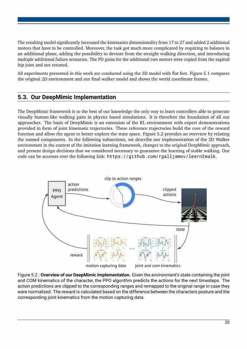
The DeepMimic framework is to the best of our knowledge the only way to learn controllers able to generatevisually human-like walking gaits in physics based simulations. It is therefore the foundation of all ourapproaches. The basis of DeepMimic is an extension of the RL environment with expert demonstrationsprovided in form of joint kinematic trajectories. These reference trajectories build the core of the rewardfunction and allow the agent to better explore the state space. Figure 5.2 provides an overview by relatingthe named components. In the following subsections, we describe our implementation of the 3D Walkerenvironment in the context of the imitation learning framework, changes to the original DeepMimic approach,and present design decisions that we considered necessary to guarantee the learning of stable walking. Ourcode can be accesses over the following link: https://github.com/rgalljamov/learn2walk.

Rustam Galljamov • IAS & Locomotion Laboratory • TU Darmstadt • July 30th 2020 1

PPOAgent

state

reward

motion capturing data joint and com kinematics

clipped actions

actionpredictions

clip to action ranges

Figure 5.2.: Overview of our DeepMimic Implementation. Given the environment’s state containing the jointand COM kinematics of the character, the PPO algorithm predicts the actions for the next timesteps. Theaction predictions are clipped to the corresponding ranges and remapped to the original range in case theywere normalized. The reward is calculated based on the difference between the characters posture and thecorresponding joint kinematics from the motion capturing data.

20

5.3.1. State and Action Space

State Space. The state of our environment consists of joint angles and angular velocities in Cartesian jointspace as well as COM position and velocities. The COM position in the walking direction (x axis) is notincluded in the state observations, to make the controller independent of the walked distance. We chooseto specify joint kinematics which are easier to measure in a robotic system instead of the relative positionand orientation of the character links proposed by Peng et al. (2018a), which are more common in computergraphics.Besides the kinematics of the current timestep we include the desired walking velocity and a phase variable φindicating the start and the end of a step cycle. Desired velocity is calculated from mocaps as the averageCOM forward velocity during a step. The phase variable is a monotonically increasing scalar value in the range[0, 1] indicating the start of a step by φ = 0 and the end by φ = 1.End effector positions were left out. One main reason for including this information was to avoid idiosyncraticmotions. These are most often produced by the hands which are not included in our model. Moreover, thisinformation is redundant as it can be obtained by forward kinematics from observed joint angles if necessary.The states are normalized dimension-wise with the corresponding running mean µi and variance σ2

i calculatedin the environment by the following formula with ϵ = 10−8 for numerical stability:

si,norm =si − µi√σ2i + ϵ

Action Space. We consider two different action types during our experiments: joint torques and target anglesfor the PD position controller in each joint proposed in the original DeepMimic implementation (Peng et al.,2018a). The policy is queried at 200Hz, thus the same control input is applied for 5 simulation frames whichis often referred to as frameskip. Actions predicted by the policy are clipped to the allowed torque or angleranges of each joint. In case of normalized action spaces, the actions are clipped to [−1, 1] and mapped to theactual ranges in the RL environment.

5.3.2. Reward Function

The reward function is like in the original DeepMimic approach a weighted sum of individual reward partsencouraging the imitation of the expert reference trajectories. We reward the agent for matching the jointpositions with rp, joint angular velocities with rv and the COM kinematics by rc. We decided against using theend-effector reward considering its high redundancy with the position reward and the absence of arms inour simulation model. The weighting of this reward component is added to the position reward. The finalimitation reward function is presented in the following equation:

r = wprp + wvrv + wcrc

wp = 0.8, wv = 0.1, wc = 0.1

The individual reward components at each timestep are calculated by comparing the difference between theappropriate values x in simulation with the corresponding values on the reference trajectories x as follows:

ri = exp[−αi(∑j

∥xj − xj∥2)]

αp = 3, αv = 0.05, αc = 16

21

x takes the role of joint angles for the position reward rp, stands for joint angular velocities in rv andcorresponds to COM position and linear velocities within rc. The scaling factors αi in each reward componentare tuned by hand until the reward for different deviations corresponded with our subjective rating.By using the exponential function with negative exponents, having a minimum deviation of 0, and choosingthe weights of the individual reward components to sum up to 1, the reward at each timestep lies in the range[0, 1]. To encourage longer episodes and thereby falling avoidance, an alive bonus is added to the imitationreward at each step. The bonus is chosen as 20% of the maximum possible step reward.

5.3.3. Episode Initialization and Termination

The way an episode is initialized and terminated has been shown to drastically influence the learning speedand performance (Peng et al., 2018a). We consider both recommendations in the framework of DeepMimicand implement Early Termination (ET) and Reference State Initialization (RSI). While RSI is adopted withoutchanges, we change the trigger criteria for ET as well as the calculation of the reward in terminal states.Initialization. Each episode is initialized in a state uniformly sampled from the available mocap data.Therefore, we randomly select one of the steps from the expert demonstrations. Then, we randomly selectone point on the step trajectories and use the corresponding reference kinematics to set the initial COM andjoint position and velocities in the simulation. This procedure allows the agent to explore all parts of the statespace from the training’s beginning on leading to quicker convergence.Episode Termination due to Maximum Duration. Even walking is a cyclic motion and should be framedas an infinite horizon MDP, it is common to define a maximum episode length to diversify the collectedexperiences (Reda et al., 2020). We terminate the episode after a maximum amount of 3k steps. Given ourcontrol frequency of 200Hz and a minimum walking distance in the expert demonstrations of 1.4m/s, theagent is provided with enough time this way to walk at least 21 meters.Peng et al. (2017) do not report a special treatment of the reward calculation in the terminal state due tomaximum episode duration. It is likely they don’t distinguish between terminal and non-terminal states.Treating the terminal step the same as all previous steps however, results in the same state-action pair gettingdifferent returns and thus ratings based on where in the episode they occur. Accordingly, good actions takenat the episode’s end get rated badly and result in contradicting experiences the policy has to learn from (Pardoet al., 2018).Pardo et al. (2018) investigated different time limits in reinforcement learning and confirmed the importanceof correctly treating terminal states. They propose to estimate the return of the terminal action by queryingthe Q function which approximates the cumulative discounted future return of state-action pairs.To reduce implementation effort and put more focus on optimizing sample efficiency, we decided to approximatethe return of the terminal action from current training statistics. Therefore, we maintain a running mean ofthe reward during training rt and use it to calculate the average cumulative future return of an average actionusing the maximum episode duration and the discounting factor γ. This value, which is calculated as follows,is then used as a simple to calculate estimation of the expected return in the terminal state Rt

ˆ .

RT =

[T∑t=0

γtrt

]

22

Table 5.2.: Early Termination Conditions. The table summarizes the maximum allowed deviations in trunkangles (in radians) and COM positions (in meters) before we stop the episode early. The trunk angles inthe sagittal and frontal plane as well as the COM Z position indicate early falling detection. COM Y and thetrunk angle in the traverse plane a deviation from straight walking.

TrunkSaggital

TrunkFrontal

TrunkTransverse

COM Y COM Z

Max Allowed 0.3 0.2 0.5 0.15 2.0Min Allowed -0.05 -0.2 -0.5 -0.15 0.95

The proposed way to calculate the reward on the end of an episode allows to freely change the reward function,the scale of the reward, and the episode duration, without the need to adapt other hyperparameters.Early Termination. The authors of the DeepMimic approach stop the episode early when the trunk or thehead of the animated character touch the ground. The reward for the terminal state is set to 0 (Peng et al.,2018a). Using this terminal condition and reward, we observed the agent to not always converge to stablewalking. Avoiding falling however is more crucial than human-like appearance when complex and expensiverobotic hardware is concerned, which is why we changed the terminal conditions and decided to punish fallsmuch harder.Our termination criteria is based on early falling detection indicated by a low COM position or significantdeviations from the desired trunk angles in all three directions. In addition, we stop the episode whenwalking direction changes above a certain threshold to guarantee straight walking. Table 5.2 summarizes theallowed trunk rotations and COM heights before falling or direction changes are detected and the episode isterminated.In addition to terminating the episode earlier, far before the character has touched the ground with its head ortorso, we observed it as necessary to provide clear negative feedback in form of a negative reward on terminalconditions. Choosing an appropriate reward turned out to be challenging. Punishing falling lightly with areward of -1 or -10 had no significant impact on the learned walking stability. Punishing falling with -1000which is close to the maximum possible episode return resulted in stable walking however took much longerto converge.We explained the delay in convergence when using high negative rewards to punish falling as being toohard for the short episodes at training’s beginning which result in a maximum return of 50. This way, allactions in the episode had a similar negative return and even good actions were rated badly resulting in aweak training signal slowing down policy improvement. The cause for the absence of convergence in case ofthe low punishments was understood to be an unclear signal to avoid falling. Therefore, we implementedan adaptive ET reward by maintaining a running mean of the episode return and using the negative of forterminal conditions. Following this approach, the agent converged to stable walking almost without exceptionsmaintaining high sample efficiency.

23

5.3.4. PPO Hyperparameter Choices

We use the stable-baselines implementation of PPO (Hill et al., 2018) in version 2.10.0. It builds uponTensorFlow 1.14 (Abadi et al., 2015) and supports parallelization and the use of a GPU (PPO2). All usedpackages and their versions are listed in the appendix APX. We use default hyperparameters where possibleand specify them otherwise in this Section. An AMD Ryzen Threadripper 2990WX processor with 32 cores isused to collect experiences and an Nvidia GeForce GTX 1080 Ti GPU for updating the network weights.We train our agents on two variations of the 3D walker environment, one having torque controlled joints andthe other using PD position servos to track desired joint angle trajectories. All considered action spaces arenormalized to the interval [−1, 1]. The hyperparameters were tuned using the torque controlled model. TableX summarizes the most important hyperparameters.The torque model is trained for 8M timesteps, the PD controlled model for 16M timesteps. We collect a batchof 32k experiences with a fixed policy and perform 4 optimization epochs using Adam (Kingma and Ba, 2014)splitting the data in minibatches of 2k samples. The experiences are collected on 8 parallel environments,each using a different random seed. The VecNormalize environment from stable-baselines is used to collectthe states and returns of all parallel environments and calculate running statistics for normalizing both ofthese values.We use the same network architectures with two hidden layers of 512 units for the value function and thepolicy with the exception of the number of outputs, which is 8 for the latter and 1 for the former. Even Penget al. (2018a) propose to use 1024 and 512 units in hidden layers, networks with the same number of units inhidden layers always performed better during hyperparameter tuning. No hidden layers are shared betweenthe actor and the critic. ReLU (Glorot et al., 2011) is used as the activation function in all layers except forthe output layers which have linear activation. We use orthogonal initialization of the network weights andscale these down by a factor of 0.01 after initialization. Especially the scaling of the policy’s output layer wasreported to be important, making the initial action distributions symmetric around zero and independent ofthe states (Andrychowicz et al., 2020). The orthogonal matrix is obtained by QR decomposition of a matrixwith entries randomly sampled from a normal Gaussian distribution.All considered action spaces are normalized to the range [−1, 1] for better comparison. The initial standarddeviation of the Gaussian policy is set to 0.5 allowing sufficient exploration of the normalized action space.With this choice, only 4.55% of actions lands outside the allowed normalized range. In contrast, when usingthe default standard deviation of 1 in combination with zero means and normalized action spaces, 27.18%of sampled actions will be outside of the allowed range. Actions outside the range will be clipped to theboundaries and therefore result in an unevenly distribution of actions across the whole space.To avoid early collapsing to a deterministic policy and continue exploration until the end of the training, thestandard deviation is bounded to the interval [0.1, 1]. On the other side, too high exploration after convergenceto stable walking has been observed to regularly harm the stability. Therefore, we add an entropy punishmentwith a coefficient of 0.0075 resulting in a smooth decay of the exploration during training that has proven topositively influence convergence behavior and walking stability.The learning rate is linearly decayed over the course of the training starting with 5× 10−4 and ending with1× 10−6. Finally, the performance of the learned controller is crucially influenced by the discounting factorγ. To choose an appropriate value, we used the formula γ = exp(−1/τ) with τ specifying the consideredtime horizon in number of agent-environment-interactions after which the influence of actions on the returnis exponentially decreased (Wright, 2019). The best results were achieved considering a time horizon of 1second - 200 steps at a control frequency of 200Hz - with the corresponding discounting factor γ = 0.995.

24

5.4. Sample Efficiency Evaluation

In this section, we present the performance metrics used for the evaluation of the sample efficiency in thecontext of learning human-like bipedal walking. Next to conventional metrics, the Summary Score is introduced,a new metric developed in this work to evaluate the sample efficiency of learning bipedal walking consideringthe human-likeness of the learned walking gait as well as the walking stability. At the beginning, the processof evaluating an agent’s performance is described.

5.4.1. Evaluation Procedure

To encourage exploration of the state and action space, reinforcement learning agents are trained using astochastic policy. After training, the stochastic components are removed and a deterministic version of thesame policy is used from now on to accomplish the desired task. It is therefore important to evaluate thedeterministic policy. Typical learning curves however show the average performance of the stochastic policyduring training. Moreover, when training in multiple parallel environments, the performance metrics areaveraged over all environments. A low return due to falling in a single of the parallel environments wouldtherefore only insignificantly reduce the metric, averaging out the important information of a fall and hidingthe fact of the policy not being fully stable.Considering the listed scenarios, we propose the following evaluation procedure. We pause the training inregular intervals, load the current policy and evaluate it in a deterministic manner in a single environment usingthe outputted means of the Gaussian action distributions as predictions. The agent’s behavior is monitored for20 episodes, initializing each in a different step from the reference data.The initial phase of the step cycle is chosen to be 75%. This way, we avoid initialization in states rich in contactand impacts which are hard to model precisely. At 75% of the step cycle we are no longer in the doublesupport phase halving the contacts and are maximally far away from touchdown and takeoff characterized byhigh impacts.The evaluation intervals are chosen as follows. For the first 1M timesteps of training, evaluation is performedevery 400k steps, allowing 10 policy updates. After the agent reaches an average walked distance of 5 metersduring evaluation, we reduce the interval to every 200k steps and to 100k after 10 meters are reached.After surpassing 20 meters, the interval is again increased to 400k to avoid longer training durations due tofrequently repeating evaluations.To make the curves of individual agents easier to compare, we smooth them using exponentially weightedsmoothing with a smoothing factor of 0.25. In detail, the smoothing is achieved by weighting the returns ofprevious episodes with exponentially decreasing weights and using their sum instead of the return for thecurrent episode.

5.4.2. Performance Metrics for Sample Efficiency Evaluation

In reinforcement learning, sample efficiency is generallymeasured as the number of required agent-environmentinteractions until a specified performance threshold is reached. This section answers the question of howto measure the performance of an agent learning to walk stably in a visually human-like fashion as well ashow to choose an appropriate threshold. We start by explaining why the return as an obvious performancemeasure is not suitable for the specific case we consider.

25

Episode Return. The obvious performancemeasure in a reinforcement learning setting is the return, calculatedas a discounted cumulative sum of future rewards. In our case, the reward measures the similarity betweenjoint and COM trajectories in simulation with the motion capturing data. By punishing falling with a highnegative reward, the return also implicitly covers the walking stability which is crucial when training robotsto walk. A detailed reward formulation is presented in Section 5.3.2.However, the return based sample efficiency will be highly dependent on the defined threshold which is hardto specify fairly as following examples portraits: Consider an agent that learns to walk stably reaching 70% ofthe return after 4M steps and reaching 80% after 10M steps. Another reaches 70% of the return after 6M and80% after 8M experiences. Setting the threshold at 70%, the first agent is 2M samples more efficient, settingthe threshold at 80% the second leads with the same advantage. In addition, the return curve is often verynoisy, making it more difficult to specify a suitable threshold and compare the approaches.Combine two metrics to measure sample efficiency evaluation. To consider the walking stability, weobserve the agent over 20 consecutive episodes during evaluation and count the number of times the balancewas successfully kept until the end of the episode. We call this metric the Number of Stable Evaluation Walks.The episode duration is set to 15 seconds giving the character enough time to reach 22.5 meters whenfollowing the desired walking speed of 1.5m/s. To consider the human-likeness of the learned walking gait,we record the average imitation reward over the 20 evaluation episodes.To consider both metrics at the same time we need to specify a threshold for each of these graphs. Thethreshold for stable walks is set to the maximum 20 episodes. Empirically we’ve observed a reward of 50% tobe enough to achieve visually human-like walking. If we want to guarantee close imitation of the referencetrajectories, we can specify the threshold at 75%. Please note that reaching 100% is impossible in practicedue to differences in morphology, contact dynamics and alike. The maximum achieved reward during ourexperiments was 82%. As a first sample efficiency metric we then obtain the number of sampled experiencesuntil the agent accomplishes to walk stably while replicating the expert trajectories to an satisfying degree.We define stable walking as reaching the episode’s end without falling on all 20 evaluation episodes.

5.4.3. Convergence Stability

During our experiments we observed that policies generating stable walking occasionally diverge from thestable behavior if they’re trained further. After a following policy update, they are no longer able to reach theepisode end on all 20 evaluation runs without falling. The third approach in Figure 5.3 (a) illustrates thisbehavior. We explain this fact of having learned a policy that has converged to an unstable local optimum.Such a policy is expected to generalize poorly to unseen or noisy states and is therefore undesirable. Therefore,this behavior is important to be considered and is worth giving it a name.In the context of this work, the term convergence behavior is always referring to the number of stable evaluationwalks after reaching stable walking for the first time. The convergence is stable, when the agent continues towalk stably after future changes to the policy, hence the number of stable walks remains at 20. It is unstable,when the stable walks curve drops as the agent starts falling on some of the evaluation episodes after futurepolicy updates.

26

5.4.4. Summary Score Metric

Given the argumentation in previous sections, an optimal metric measuring the sample efficiency of algorithmsaiming at learning stable walking should consider the following points:

1. How quickly does the agent achieves stable walking for the first time?2. How human-like does the character move?3. How do the first two metrics change when policy is trained further (convergence behavior), e.g. to

further improve human-likeness or robustness of the learned walking gait?The area under the learning curve has been previously proposed as an estimator for the learning speed (Pengand van de Panne, 2017). To fully include the human-likeness and walking stability in our evaluation, weneed to consider two different learning curves: the number of stable evaluation episodes and the average stepreward during evaluation. As human-like walking without stability is of no interest and stable walking that isnot human-like is undesired, we multiply both curves pointwise and compute the area under the resultingcurve.To significantly punish divergence from stable walking reflected by drops in the number of stable evaluationepisodes, we take it to the power of 4. To also clearly punish deviations from expert demonstrations but stillconsider the higher importance of stability over human-likeness, the reward is taken to the power of 2 only.The final metric is calculated with the following formula:

SumScore(nt, rt,T) :=100

T

∫ T

0(nt

20)4 r2t dt (5.2)

T denotes the whole training duration in samples, nt the number of stable walks and rt the average stepreward during an evaluation. 100/T normalizes the score to the range [0, 100] given the maximum summaryscore per timestep is 1. When the summary score is computed during training, it results in a monotonicallyincreasing curve clearly rating different approaches at the end of the training.

0 4 8 12 16 20

0.0

2.5

5.0

7.5

10.0

12.5

15.0

17.5

20.0

(a) #

Sta

ble

Wal

ks

0 4 8 12 16 20

0.2

0.3

0.4

0.5

0.6

0.7

0.8

(b) M

ean

Eval

uatio

n R

ewar

d

0 4 8 12 16 20

0

5

10

15

20

25

30

(c) S

umm

ary

Scor

e

Approach 1Approach 2Approach 3

Training Timesteps [x106]

Figure 5.3.: Advantages of Using the Summary Score 3 Approaches are compared: Quick convergence ata low reward (1), same time to convergence at a higher reward (2), and quickest convergence at highestreward, but diverging from stable walking (3). Where it is hard to specify thresholds for the first two graphsto correctly rate the three approaches, the final summary score reflects our rating correctly and distinctly.

27

Figure 5.3 shows the summary score together with the learning curves used for its calculation. The curveswere specifically generated to highlight the advantages of our metric. Looking at the number of stable walksalone (a), the first two approaches perform equally well. The summary score (c) considers the higher rewardsof the second approach and rates it significantly better compared to the first.Approach 3 illustrates the punishment of a bad convergence behavior. The agent is the earliest to achievestable walking. However, the performance diverges during the following policy updates and the agent is nolonger able to maintain the balance on all 20 evaluation walks (a). Despite also achieving a higher rewardduring the whole training duration (b), this approach is rated second after the orange approach which showsa significantly better convergence behavior.

5.5. Approaches to Improve Sample Efficiency of DeepMimic

Our first attempt to sample efficient learning of bipedal walking was to adapt the DeepMimic approach for ourspecific learning scenario. After this was accomplished, our focus changed to further improving the sampleefficiency over this baseline. Figure 5.4 shows an overview of the considered approaches shortly summarizedin the following.Using PD position servos in the joints as proposed by the authors of DeepMimic (Peng et al., 2018a), it waspossible to generate state-action pairs out of the reference trajectories and pretrain the agent in a supervisedmanner, an approach known as Behavior Cloning. Next, we investigated the influence of different actionspaces on learning speed and performance.Considering the results of previous experiments, our second group of approaches were implemented using thetorque controlled walker model. The goal here, was to induce prior knowledge about the task in the learningprocess. We considered the symmetry of the desired motion and included additional information into thestate observations. Finally, we tested techniques proven effective in the context of deep or deep reinforcementlearning including experience replay, dimensionality reduction and hyperparameter scheduling.

Improving the Sample Efficiency of DeepMimic for Bipedal Walking

Adaptations to the DeepMimic Approach

Policy Initialization with Behavior Cloning(Section 5.6.1)

Action Spaces Comparison(Section 5.6.2)

Induction of Prior Knowledge Adaptations to the PPO Algorithm

Experience Replay(Section 5.6.5)

Exponential Cliprange Decay(Section 5.6.6)

Considering the Symmetry of Walking(Section 5.6.3)

Adding Ground Contact Information(Section 5.6.4)

Figure 5.4.: Overview over Considered Approaches to Improve Sample Efficiency. We consider multiplemethods targeting at improving the sample efficiency of our DeepMimic implementation. The approachescanbe categorized in changes to theDeepMimic approach, incorporation of prior knowledge into the trainingprocess as well as adaptations to the PPO algorithm.

28

5.5.1. Better Initial Policy with Behavior Cloning (BC)

Analyzing the outcomes of our first experiments, we observed all learning curves to show a very slowimprovement for quite a significant duration after the training’s start. We explained these observation by therandom weight initialization leading to a poor initial policy that is far away from being even sub-optimal. Ittook a high number of updates to bring the policy in a shape to quicker improve the performance.To improve the initial policy, we decided to pretrain it on the reference trajectories in a supervised manner.This approach is known as Behavior Cloning (BC) (Schaal, 1997) and has been often applied in the field ofrobotics (Atkeson and Schaal, 1997; Argall et al., 2009; Kober and Peters, 2010). The basis of this approachare expert demonstrations in form of state-action-pairs. When we use the walker model with position servosin each joint, our policy observes the joint kinematics of the current timestep and has to predict the jointpositions at the next point in time. In this case, it is easy to generate state-action-pairs from the referencedata and use it to pretrain the policy.Even knowing the approach is likely to fail as proposed by the literature (Ross et al., 2011), BC is a must-tryapproach when aiming at higher sample efficiency. When succeeding, it allows to pretrain the policy in afully supervised manner without a single agent-environment interaction. Moreover, the drawbacks of purebehavior cloning were planed to be compensated by combining it with reinforcement learning (Kober andPeters, 2010). We expected the pretraining on mocap data to either produce useful features that will speed uplearning process in a transfer learning fashion (Pan and Yang, 2010) or less likely already learn a near-optimalpolicy. This policy was expected to overfit to the state distribution in the expert demonstrations (Ross et al.,2011), but should be improved by continue training it in a reinforcement learning setting.The value function network could have also been pretrained from expert demonstrations. However, since thevalue function loss quickly converged to zero during training and was unlikely the bottleneck to better sampleefficiency, we haven’t considered this scenario in our experiments.Generation of the Supervised Learning Data Sets from Reference Data. To pretrain the policy, we needto transform the expert reference trajectories into state-action-pairs. The policy for the PD position controlledmodel gets the current environment state as input and outputs desired joint angles for the next timestep asactions. The state consists of joint and COM kinematics as well as the desired walking speed and a phasevariable. The extraction of this information from the reference data is straightforward. The actions specify thetarget joint angles at the next timestep and are estimated from the next point on the mocap trajectories.The generated dataset was shuffled to decrease the violation of the i.i.d. assumption due to states beinginfluenced by former actions (Ross et al., 2011). Finally, we split the data in a train, validation and test setusing 80, 10 and 10 percent of the data respectively. After the hyperparameters were tuned, we merged thevalidation and training set.Pretraining of the Policy Network. To implement BC, the Keras module of the TensorFlow framework (Abadiet al., 2015) is used. We build a fully-connected neural network having the same size and activation functionsas the policy network used in PPO. The weights of the network are also initialized as an orthogonal matrixwith entries scaled down by 0.01.After comparing different loss functions the Mean Absolute Error (MAE) was chosen to be minimized duringpretraining. We trained the network for 200 epochs and used Adam (Kingma and Ba, 2014) with linearlearning rate decay from 0.01 to 0.0005 for the weight optimization. Even the learning curves didn’t signalsignificant overfitting, we still utilized L2 regularization (Ng, 2004) with a coefficient of 0.0005 hoping for

29

better generalization to unseen states. The absence of overfitting can be explained by the high variance in thedata with all steps having slightly different trajectories as can be seen in the appendix (Figure A.2).Usage of the trained model. After training the model to output desired joint angles for a given state on thereference trajectories, we save the model parameters. During the network initialization step of PPO, we thenload the pretrained network instead of initializing a new random network and begin the training. During thisstep, we tried loading only the hidden layers of the pretrained network as well as the whole network usingthe outputs as the mean actions of a Gaussian distribution.

5.5.2. Sample Efficient Action Spaces

Peng et al. (2018a) propose to use target angles for PD controllers in each joint as the agent’s action. Next tothis action space, we also investigate outputting joint torques as well as differences to the current joint angleswhich are added to the current posture to determine the target angles for the PD servos. We abbreviate thelatter approach with outputting angle deltas.Drawbacks of the Target Angle Space. Outputting target angles is expected to often result in unrealistictarget angles. The policy can output a desired angle of 45◦ even the current angle is currently at −30◦. Thepolicy however is queried at 200Hz allowing only 5 milliseconds to reach the desired angle. In this time, themotors realistically are only able to change the current joint angle by a small amount. Moreover, the targetangles of consecutive time steps can vary a lot resulting in very noisy sequences like [0◦, 120◦,−30◦, 40◦, ...].Thus, when target angles are outputted by the policy, there is a high chance to make unrealistic predictions.Besides being unreachable, unrealistic target angles come with multiple drawbacks. PD controllers choose themotor torque by scaling the difference between the current and desired joint position (Equation 5.1). Is thisdifference high, the joint torques are high too. After surpassing a certain difference threshold, the motorswill go into saturation and output the maximum peak torques. In a real robotic system, this results in highenergy consumption and significant wear of drive train components. High sudden torques are in additionlikely to have a perturbing effect on the system and prevent stable walking. Finally, joint angle trajectorieswill be unsmooth and jittering motions get highly probable.Outputting angle deltas for realistic target angles. To avoid unrealistic target angles, we propose to outputangle deltas: small angle differences which are added to the current joint positions to obtain the target anglesfor the next timestep. By choosing an appropriate maximum angle difference, the risk of target angles thatcannot be reached can be drastically reduced or fully eliminated. We expect this approach to significantlyimprove the smoothness of the joint trajectories, reduce motor torques and increase the quality of the learnedmotion. More importantly, this approach promises to increase the learning speed by strongly limiting theaction space at each point in time to only angles close to the current joint configuration.To output target angle deltas, the maximum possible angle differences for each joint have to be specified.These hyperparameters can be easily estimated from the reference trajectories by looking at the maximumangular velocities of individual joints. To consider out-of-distribution states requiring higher torques and to beable to recover from perturbations, we scale up the maximum velocities observed in the mocap data. Aftertesting different values, a scaling factor of a = 4 was declared to be the best choice.The maximum possible angle differences further depend on the time interval between two control steps.Therefore, the maximum possible velocities, specifying the angle change per second, have to be scaled downin proportion to the control frequency fCTRL. The higher the control frequency, the smaller the time betweentwo control commands and the smaller the possible change in the angle. The following simple formula sums

30

up the calculation of the individual maximum delta angles ∆qmax from the corresponding maximum jointvelocity, denoted by vmax:

∆qmax = avmax

fCTRL(5.3)

To guarantee a fair comparison, we normalize all action spaces to the range of [−1, 1] and remap the predictedactions within the environment to the specified joint, torque or delta ranges. The standard deviation for alljoints is uniformly initialized at σ2 = 0.5. With the initialization of the action means around zero (Section5.3.4), this choice allows to sufficiently explore the whole action space, exceeding its bounds with a probabilityof only 4.5%.

5.5.3. Symmetry Prior Induction

Bipedal locomotion in humanoids is a symmetric motion w.r.t. the sagittal plane. In this Section we presenttwo possibilities proposed by Abdolhosseini et al. (2019) to induce this prior knowledge in the training process.Before that, we explain the required transformations to mirror experiences given their representation as a onedimensional state vector. The vector contains the joint position and velocities as well as COM kinematics, thedesired forward velocity and the phase variable (see Section 5.3.1 for details).To mirror the state vector, we have to:

• swap the left leg joint kinematics with their correspondences from the right leg and• negate the hip angles in the frontal plane.• The phase variable and desired velocity remain unchanged. COM kinematics as well as trunk angle and

angular velocities also stay at the same position in the state vector.• The COM displacement in y-direction, the trunk angle around the x and the z-axes in addition change

their signs.• The same applies for the corresponding COM and trunk velocities.

Mirroring the action vector is much easier, requiring only to swap the left leg action positions with the rightleg actions and negate the actions of the hip in the frontal plane. In the context of this work, we denote (s′t, a′t)as the mirrored state-action pair of (st, at) at a given timestep t.Due to asymmetries in every human walking style, the collected trajectories cannot be fully symmetric. Totest the effect of asymmetry in the expert demonstrations, we conduct our experiments using the originalreference trajectories as well as the artificially symmetrized version.1. Duplicating and Mirroring Made Experiences (DUP). Joint angle and angular velocity trajectoriescollected during taking a step with the left leg can be mirrored to get the corresponding trajectories ofa step with the right leg. Therefore, it is possible to generate additional artificial experiences from trueagent-environment interactions. This approach is similar to data augmentation techniques used in supervisedlearning (Shorten and Khoshgoftaar, 2019).To duplicate the amount of training data following this approach - hence the abbreviation DUP - we needto estimate additional information about the mirrored experiences. Besides states and actions, our deep RLalgorithm PPO requires the resulted return of the state-action pair R(st, at), the value of the observed stateunder the current policy V π(st) as well as the negative logarithm of the action probability −log[π(at|st)].

31

We implement two ways to approximate the required values for the mirrored experiences. Within the firstattempt, we let the agent collect a batch of experiences (st, at, rt, st+1) and calculate the discounted returnsR(st, at), the state values V π(st) and the negative log probabilities of the actions in corresponding states−log[π(at|st)]). We then mirror the states and actions and copy these values for the mirrored states andactions. This decision implicitly makes the very strong assumption of mirrored states having the same valueunder the current policy and mirrored actions having the same probabilities as the originally predicted actions:π(a′t|s′t) = π(at|st) and V π(s′t) = V π(st).In the second approach, we query the value function and the policy networks to calculate the true state valuesand action probabilities under the current policy. To get the state values, we load the current value functionnetwork weights, including the bias terms, stack the mirrored states into a matrix and perform the requiredmultiplication operations, considering the activation functions of the network layers. This way, we get a moreprecise value estimate for the mirrored states under the current policy.The procedure of getting the true action probabilities is similar. First, we load the current policy networkweights and biases as well as the standard deviation of the action distributions. The stacked mirrored statesare then propagated through the policy network giving us the means of the Gaussian action distribution foreach state. Given the distribution, we calculate the negative log probability of the mirrored actions and usethese in the PPO update.Without further changes, this approach rarely crashes the training due to NaNs in the policy update equations.The reason for that is the near zero probability of some of the mirrored actions. We work around this issue byclipping the action probabilities to an acceptable range or delete experiences with mirrored actions that areimpossible to occur under the current policy. The threshold for the minimum considered action probability isset to one fifth of the minimum probability of the actions in the observed trajectory τ :

pmin(a′t) =

1

5min

(at,st)∈τπ(at|st)

Phase-based Mirroring (PHASE). The joint and COM kinematics of a step with the left leg are identical withthe mirrored kinematics of a step with the right leg. Another approach to consider the symmetry of walking istherefore to train the policy only outputting actions for stepping with the left leg. To get the actions for thestep with the other leg, the observations are mirrored, corresponding actions are calculated and then againmirrored to get the actions for the counterpart leg. The big advantage of this approach is the very simpleimplementation and the high generalization of the approach to other algorithms as the changes are exclusivelyimplemented in the environment.

5.5.4. Adding Ground Contact Information to State Observations

The walking motion can be split into multiple phases. The contact of both feet with the ground plays a crucialrole in determining the individual phases (Li and Dai, 2006). Therefore, we want to investigate how addingthe ground contact information to the state observation will influence the sample efficiency of the learningprocess as well as the final walking performance.We extend the state space by a binary flag for each foot indicating if it has ground contact or not. Next tobinary values, we also investigate a value of −1 to indicate the absence of contact. Further, we try introducinga separate flag for the double stance phase where both feet are in contact with the ground. In this scenario,we compare the usage of a three dimensional binary vector indicating the double stance phase by (0, 0, 1)T aswell as a dense vector completely filled with ones when both feet touch the ground.

32

5.5.5. Experience Replay Despite Being On-Policy

One of the reasons preventing a higher sample-inefficiency of the PPO algorithm is its on-policy nature,allowing it to use only data collected by the current policy to update the network parameters. Experiencescollected with previous versions of the policy are no longer suitable to estimate the gradient of the currentpolicy, increasing the need for more agent-environment interactions. Off-Policy algorithms which are notlimited by that constraint, often store experiences collected with previous versions of the policy in a replaybuffer and use them multiple times improving the sample efficiency.Being a trust region method, we can use PPO with a small clip range and guarantee consecutive policies tobe similar to each other. This way it might be possible to reuse prior experiences to estimate the gradient ofthe current policy. In this work, we want to investigate if former experiences can be used to improve sampleefficiency and if so, how many prior experiences can be maintained until the policy gradient can no longer becorrectly estimated.To answer these questions, we save collected experiences in a replay buffer. An experience is a tuple consistingof a state-action pair (st, at), the corresponding return R(st, at), the predicted state value under the currentpolicy V π(st) and the negative log probability of the taken action −log[π(at|st)]. The buffer is implementedas a first-in last-out queue that is shortened to the specified buffer size after each update. Newly collectedexperiences are merged with those from previous iterations into a new batch. Minibatches are then uniformlysampled from this mixed collection of fresh and previous experiences and used to update the policy.To maintain the same batch and minibatch sizes for a fair comparison, we decrease the number of collectedexperiences per batch by the number of considered batches per update, being one more than the buffersize. A simple implementation of the replay buffer reuses prior experiences with the state values and actionprobabilities calculated with the old policy and value function: V πold(st) and −log[πold(at|st)]. These valuesare expected to deviate from true values the older the policy the experiences were gathered with. To correctfor these deviations, we can query the current policy and value function networks to update the values andprobabilities of past experiences as described in Section 5.5.3.

5.5.6. Exponential Cliprange Decay

PPO builds upon trust region policy methods and limits the change in action distributions of consecutivepolicies. Instead of constraining the KL-divergence, this algorithm defines a clipped surrogate objectivefunction defined in Equation 4.1. The maximum allowed change is controlled by the cliprange ϵ which weschedule to exponentially decrease over the course of the training from 0.55 to 0.1 with the following formulawhere T denotes the training duration:

ϵ(t) = 0.1 + 0.45 e−5t/T

Our motivation for the exponential decay of the cliprange is the following. As the policy is initialized withrandom weights, it performs poorly at the training’s beginning. Tens to hundreds of updates are necessaryto result in a near-optimal behavior. By restricting the maximum possible behavior change during a policyupdate, the number of required updates further increases. Choosing a high cliprange can help quickly improveupon the random policy. As far as the policy however reaches near-optimal performance, big changes to theaction distributions can have a destructive effect on the policy’s behavior and thus should be limited. Anexponentially decaying schedule allows big changes to the initial random policy, moderate changes during thefollowing early stage of the training and finally strongly limits the difference of consecutive policies as theagents performance increases.

33

6. Results

We evaluate each approach on a minimum of 5 different random seeds. The number of required samples toconvergence portraits the whole distribution over the experiments as a violin plot. All other curves show themean and one std over the seeds.For each approach we in addition report two groups of learning curves. The first focuses on metrics usedto evaluate the sample efficiency. With the exception of the episode return, the three other subfigures arecollected during deterministic evaluation of the current policy (Section 5.4.1). From left to right, the graphsshow:

1. Number of stable walks out of 20 evaluation runs as a measure for the walking stability and convergencebehavior.

2. Mean step reward during the 20 evaluation runs approximating the average similarity of produced jointand COM trajectories with the expert demonstrations. We highlight the achieved reward at convergenceas well as the required time to achieve 75% of the reward indicating visually fully human-like walking.

3. Summary Score as an overall measure for the suitability of an approach for quickly learning bipedalwalking, considering the sample efficiency in combination with walking stability and human-likeness ofthe learned walking gait.

4. Normalized episode return as the standard learning curve in deep RL.We furthermore highlighted important points for the sample efficiency evaluation on these graphs with markersand sum them up in a table: The time to convergence with corresponding reward and return values at thatpoint as well as the time required to reach an average imitation reward of 75% empirically guaranteeingvisually smooth and human-like walking. The required timesteps are computed individually for each of therandom seeds and are then averaged to get the time for an approach. The graphs however are averagedpointwise and show the mean over the 5 runs. Therefore, the highlighted convergence timesteps do notcorrespond to the point on the stable walks graphs where the mean reaches the maximum value of 20 stepsfor the first time. The same procedure causes the 75% reward markers being positioned not exactly at a valueof 0.75.The second group of curves breaks down the imitation reward obtained during training in its three componentsdescribing the imitation accuracy of different parts of the expert demonstrations: joint positions, joint angularvelocities, and COM kinematics.All metrics except of the summary score and the number of stable walks are smoothed for better comparisonusing the exponential window function with a smoothing factor of 0.25. Algorithmic design choices andhyperparameters listed in Section 5.3.4 are held constant across all implementations where possible. Exceptionsare explicitly mentioned during the results presentation.

34

6.1. Comparison of Different Action Spaces

The baseline for the following comparison is our implementation of the DeepMimic approach adjusted tomaximize its effectiveness in learning stable bipedal walking (Section 5.3). We use this framework with threedifferent action spaces: the default target angles for PD position servos in each joint, target angle deltas andjoint torques (Section 5.5.2). All action spaces are normalized to the same range [−1, 1] which is remapped tothe actual ranges before being applied to the environment.Figure 6.1 shows the distribution of required samples to achieve stable walking over 5 random seeds. Trainingthe policy to output target angles requires an average of 9.6 million interactions with the environment untilthe agent achieves stable walking for the first time. By outputting angle deltas, stable walking is achievedusing 41% less samples. In case of joint torques, the sample efficiency is more then doubled compared to thebaseline, requiring 5.1 million (53%) less samples. Therefore, the torque model training is stopped after 8million steps compared to 16 for the other approaches. The violin plots further show a reduction in varianceacross random seeds of more then 2 times when using our action spaces.Figure 6.2 compares the learning curves of the considered action spaces highlighting the points importantfor the sample efficiency evaluation. Our proposed action space achieves significantly better scores across allconsidered metrics with the torque model outperforming the angle deltas. The average evaluation reward andthe training return are at all points in time higher compared to the baseline.The number of stable walks (a) underlines the earlier convergence of our approaches. The baseline modelreaches the first stable walks almost at the same time as the other two approaches. Our action spaces thereafterhowever, require less than 2 milliion timesteps to converge to fully stable walking while the baseline shows amore then twice slower improvement and higher variance across the seeds.The evaluation reward (b) shows a significantly closer replication of the expert demonstrations throughoutthe whole training duration. At convergence, the torque approach achieves an average step reward of 66%compared to 53% of the baseline while angle deltas achieve 58%. Interestingly, the rewards of all methodscontinue to rise after converging to stable walking. However, only our methods reach the 75% reward,empirically guaranteeing a visually human-like walking gait. Even after 16 million steps, the baseline onlyreaches an average episode reward of 69%.

Target Angles(Baseline)

Angle Deltas(Ours)

Joint Torques(Ours)

4

6

8

10

12

Step

s to

Con

verg

ence

[x10

6 ]

9.6M

5.7M

4.5M

Figure 6.1: Sample Efficiency of dif-ferent action spaces. The violin plotsshow the distribution of requiredagent-environment interactions untilthe agent achieves stable walking.Stable walking is defined as walking20 meters on 20 consecutive evalua-tion episodes without falling. Lowernumbers correspond to better sampleefficiency.

35

Table 6.1.: Sample efficiency comparison. Both our approaches achieve better values across all metricswith the torque model performing the best. Convergence is defined as learning to walk without falling. 75%of the maximum reward indicate visually human-like walking.

Approach SummaryScore

Steps toConvergence

Reward atConvergence

Steps to75% Reward

FinalReward

Target Angles 7.2 ± 1.0 9.6 M ± 1.2 M 0.53 ± 0.05 not reached 0.69 ± 0.03

Angle Deltas (Ours) 15.1 ± 0.7 5.7 M ± 0.5 M 0.58 ± 0.05 7.2 M ± 0.5 M 0.81 ± 0.01

Joint Torques (Ours) 23.4 ± 3.2 4.5 M ± 0.4 M 0.66 ± 0.06 5.1 M ± 0.4 M 0.82 ± 0.01

The summary score (c) is more than twice as high for the delta model as the baseline’s value and is morethan three times as high when outputting joint torques. The return (d) as the typical learning curve in deepRL supports the presented results and shows different values for each approach at convergence. Table 6.1summarizes the most important points on these curves and highlights the best results, all achieved by thepolicy outputting torque commands.A comparison of the individual reward components in Figure 6.3 shows a different rating of the action spaces.Both of our approaches show a higher position rewards (a) compared to the baseline after 2 million timestepsand higher velocity rewards (b) from beginning on. After 8M samples, the torque model mimics the jointpositions the best, the delta model the second best. After further training however, the angle delta managesto reach and surpass this value. Interestingly, the same model better mimics the reference joint velocitiescompared to our second approach through the whole training duration. The baseline in contrast constantlyincreases its capability to match the angular velocities but never surpasses 2% of the maximum possiblereward.

0 4 8 12 160.0

2.5

5.0

7.5

10.0

12.5

15.0

17.5

20.0

(a) #

Sta

ble

Wal

ks

0 4 8 12 16

0.1

0.2

0.3

0.4

0.5

0.6

0.7

0.8

(b) M

ean

Eval

uatio

n R

ewar

d

7.25.1

0 4 8 12 16

0

5

10

15

20

(c) S

umm

ary

Scor

e

0 4 8 12 16

0.0

0.2

0.4

0.6

0.8

(d) N

orm

aliz

ed E

piso

de R

etur

n

Target AnglesAngle Deltas (Ours)Baseline

Training Timesteps [x106]

Figure 6.2.: Benefits of changing action space. We compare 3 action spaces: target angles (DeepMimic),angle deltas (ours), joint torques (ours). On all metrics, angle deltas improve upon target angles and jointtorques perform the best. Circular markers and dashed lines highlight the convergence point. X-markersand dotted lines emphasize the duration until 75% of imitation reward are reached, necessary to ensurevisually human-like walking.

36

In general, we see higher scores for matching the joint angles from the expert demonstrations compared tothe angular velocities. Moreover, all approaches start with a high COM reward which monotonically decreasesover time. The better a model performed in the learning curve comparison, the stronger the decrease.Finally, we collect the joint position and velocity trajectories of an agent from each action space on twoconsecutive gait cycles. Due to high similarity between both legs, only results of the right leg are shown. Weclearly see in Figure 6.4 (a) that the agent outputting target angles doesn’t manage to generate smooth jointvelocity trajectories. On the contrary, they are extremely noisy. Also the joint position over time includesjittering being especially high for the ankle joint. Links to videos showing the corresponding motions are linkedin the Readme file of our GitHub repository under https://github.com/rgalljamov/learn2walk.Our action spaces in contrast, displayed in Figures 6.4 (b) and (c), generate smooth joint angle trajectoriesvery similar to the once from the mocap data. Even the angular velocity trajectories overlap significantlyless, the obtained trajectories still show smooth transitions. A significant difference in trajectory smoothnessbetween our two proposed methods is not observed. Figure 6.5 shows multiple snapshots of the charactercontrolled by the torque model.In summary, both of our approaches significantly improve across all metrics upon the baseline. The torquemodel achieves the best sample efficiency requiring 53% less data to converge to stable walking. With 5.1Msteps it also requires the least amount of samples to reach 75% of the imitation reward. When the consideredrobotic hardware is equipped with PD position servos in each joint, a higher sample efficiency is reachedby outputting angle differences instead of target angles. This action space reduces the required samples toconvergence by 38%, generates smooth joint trajectories and is able to replicate the expert demonstrationsclosely after 7.2M steps. The rating of the three compared approaches is clearly reflected in the summaryscore which evaluates the overall suitability of a method for quickly learning to walk on two legs using deepRL.

0 4 8 12 16

0.3

0.4

0.5

0.6

0.7

(a) A

vera

ge P

ositi

on R

ewar

d

0 4 8 12 16

0.0

0.1

0.2

0.3

0.4

0.5

(b) A

vera

ge V

eloc

ity R

ewar

d

0 4 8 12 160.2

0.3

0.4

0.5

0.6

0.7

0.8

0.9

1.0

(c) A

vera

ge C

OM

Rew

ard Target Angles

Angle Deltas (Ours)Joint Torques (Ours)

Training Timesteps [x106]

Figure 6.3.: Individual imitation reward components during training. Our approaches outperform the base-line in replication of joint kinematics (a,b). Angle deltas show higher velocity values, the torque model thehighest position reward during its halved training time. The baseline model stands out having an almostconstant velocity reward of 0 (b). No approach manages to match the COM trajectories (c). Circles andcrosses mark the values when reaching stable walking and 75% of imitation reward respectively.

37

0.75

0.50

0.25

0.00

0.25

1. A

ng H

ip S

agitt

al R

0.10

0.05

0.00

0.05

2. A

ng H

ip F

ront

al R

0.0

0.5

1.0

3. A

ng K

nee

R

0.2

0.0

0.2

0.4

4. A

ng A

nkle

R

1400 1600 1800 2000

5

0

5

5. V

el H

ip S

agitt

al R

1400 1600 1800 2000

2

0

2

6. V

el H

ip F

ront

al R

1400 1600 1800 2000

10

0

10

7. V

el K

nee

R

1400 1600 1800 200020

10

0

10

20

8. V

el A

nkle

R

SimulationReference

Simulation Timesteps

(a) Target Angles (Baseline)

0.8

0.6

0.4

0.2

0.0

0.2

1. A

ng H

ip S

agitt

al R

0.15

0.10

0.05

0.00

0.05

0.10

2. A

ng H

ip F

ront

al R

0.00

0.25

0.50

0.75

1.00

1.25

3. A

ng K

nee

R

0.2

0.0

0.2

0.4

4. A

ng A

nkle

R1400 1600 1800 20004

2

0

2

5. V

el H

ip S

agitt

al R

1400 1600 1800 2000

1.0

0.5

0.0

0.5

1.0

6. V

el H

ip F

ront

al R

1400 1600 1800 2000

5

0

5

7. V

el K

nee

R

1400 1600 1800 20005.0

2.5

0.0

2.5

5.0

8. V

el A

nkle

R

SimulationReference

Simulation Timesteps

(b) Angle Deltas (Ours)

0.6

0.4

0.2

0.0

0.2

1. A

ng H

ip S

agitt

al R

0.10

0.05

0.00

0.05

2. A

ng H

ip F

ront

al R

0.00

0.25

0.50

0.75

1.00

3. A

ng K

nee

R

0.2

0.0

0.2

0.4

4. A

ng A

nkle

R

1400 1600 1800 20004

2

0

2

5. V

el H

ip S

agitt

al R

1400 1600 1800 2000

1.0

0.5

0.0

0.5

1.0

6. V

el H

ip F

ront

al R

1400 1600 1800 2000

5

0

5

7. V

el K

nee

R

1400 1600 1800 20005.0

2.5

0.0

2.5

5.0

7.5

8. V

el A

nkle

R

SimulationReference

Simulation Timesteps

(c) Joint Torques (Ours)

Figure 6.4.: Smoother joint kinematic trajectories with alternative action spaces. Comparison of the rightleg joint kinematic trajectories between the motion capturing reference data (blue) and the trajectories col-lected from the models after training (orange) for two gait cycles. The upper rows display joint angles.The corresponding angular velocities are positioned below. Our approaches result in significantly smootherkinematics, especially concerning joint velocities.

38

6.1.1. Result Interpretations

Why are angle deltas better than target angles? Outputting normalized angle deltas instead of targetangles significantly improves sample efficiency, the similarity with the expert demonstrations and results inmuch smoother joint trajectories. We believe the latter is the most important observation and the reason forthe other two improvements.Our choice of the action space can be seen as a strong inductive bias guaranteeing smooth joint trajectories. Itexplicitly limits the difference in joint angles between consecutive control steps. On the contrary, outputtingtarget angles allows arbitrarily high angle difference between the current and desired angle. A high differencein joint angles between two control steps corresponds to a high desired joint velocity. By having a sequence ofhighly different target angles at consecutive timesteps like [0◦, 120◦,−30◦, 40◦, ...]we get a corresponding noisytarget velocity sequence. This is very likely the reason for the high oscillations in joint velocities illustrated inFigure 6.4 (a). These noisy trajectories are also reflected in the reward component evaluating the imitation ofjoint angular velocities. These values stay close to zero for the whole training (Figure 6.3 (b)).High deltas in addition can bring the PD controller into saturation and result in high joint torques. Suddenchanges in angle differences cause sudden high jumps in the torque. This might help to quickly recover fromundesired states but is at the same time likely to have a perturbing effect on the walker’s stability, as Figure6.2 (a) suggests. We see the model outputting target angles reaching its first stable walk almost at the sametime as our approaches. However, while our methods from here on converge to fully stable walking in under 2million steps, the baseline progresses more then twice as slowly until it manages to maintain the balance onall 20 evaluation episodes. The recovery effect of the high joint torques can explain the early achievement offirst stable walks.On the other side, sudden joint peaks are likely to perturb the bipeds balance and bring him to fall during afew evaluation episodes. We believe this to be the reason for the slower improvement of the baseline from firstto all 20 stable walks in Figure 6.2 (a). In addition, high joint torques cause high joint accelerations quicklyincreasing the joint velocities and making them spiky as seen in Figure 6.4 (a).Why are torques better then target angles? The superior performance of the torque model may result fromthe PD controller gains being sub-optimally tuned. These parameters were tuned by holding the trunk in theair without any foot contact with the ground. Next to tuning the control parameters by hand, we tried tuning

Figure 6.5.: Human-like walking with torque control. Seven snapshots of a gait cycle recorded using thefinal policy outputting joints torques. Please note the symmetry of the gait by comparing correspondingpostures during the left and the right step. Corresponding postures are three snapshots apart.

39

them using Bayesian Optimization (Frazier, 2018). This optimization resulted in a better tracking of theexpert trajectories during tuning when the trunk was in the air. However, the training performance with theseoptimized gains was always worse compared to the hand tuned controllers. We interpreted the optimizationto overfit to the flight phase and used the hand tuned PD gains for our experiments. As we expected alsothe hand-tuned gains to overfit, we significantly increased the control parameters after tuning them in theflight phase and tested if they’re able to follow the reference trajectories also during contact with the ground.However, it is very likely the gains are still not optimal and make learning more difficult.Another reason for the advantage of torque control might be the high control frequency of 200Hz. Peng andvan de Panne (2017) as well as Reda et al. (2020) also compare different action spaces for locomotion tasksand report torque control to improve with higher control rates. On the other side, higher control frequenciesresult in shorter time intervals for a PD controller to reach a desired target angle. In combination with thetarget angle space which allows outputting angles far away from the current joint positions, the target anglesare likely to be unreached which is expected to negatively influence the learning performance.A final advantage in favor of the torque model is the symmetry of the action space especially in combinationwith our specific policy initialization. The joint torque range is symmetric w.r.t. zero. When in contrastoutputting target angles, the action space is limited by the joint ranges. These are asymmetric around zero. Incase of the knee it even only allow positive values from 0 to 2.6. Our policy is initialized with normal Gaussianaction distributions for each joint as proposed by Reda et al. (2020). All action spaces are normalized to theinterval [−1, 1]. Actions outside the allowed range are clipped at the boundaries. With this setup, the torquemodel starts outputting zero torque with the highest probability and explores positive and negative torquesequally. In the case of the knee target angle however, a action of zero corresponds to 75◦ which is almostnever occurring in the reference trajectories. Moreover, one half of the sampled actions for the knee resultin even higher angles. The situation of the other joints is less critical but similar. Summarizing, the initialpolicy for the torque model performs significantly better with the corresponding action space where the sameinitialization results in a poor initial performance in the case of target angles. Figure 6.2 (b) supports thatclaim showing a lower initial imitation reward during the first evaluations.The poor imitation of the reference trajectories in the frontal plane of the hip in Figure 6.4 (secondcolumn) are expected as we haven’t tuned the PD values for the position controller in these joints but reusedthe PD gains from the sagittal plane.Joint torque vs. angle deltas. Specifying joint torques leads to better results across all but one evaluationmetric when compared with the action space outputting differences to the current angle: the average velocityreward during training (Figure 6.3 (b)). Angle deltas are equivalent to a desired joint velocity scaled bythe control frequency and are calculated based on the maximum velocities observed in the reference data(Equation 5.3). By limiting the maximum allowed angle differences, we therefore also limit the maximumtarget joint velocity. This is likely the explanation for the drastic reduction of the high oscillations reportedin Figure 6.4 (a) compared to the target model without velocity restrictions. In addition, this limitation isexpected to allow better tracking of the reference joint velocities.Velocity can be calculated by integrating the acceleration trajectory. Thus, to obtain smooth joint velocitytrajectories, the joint accelerations must not change their sign too often and abruptly. Joint accelerations aredirectly proportional to the applied joint torque. When we start with an initial policy centered around zero,the torque model has a high probability of consecutive targets being of different signs. This can explain thelower velocity reward at the training’s beginning as illustrated in Figure 6.1 (b) that the torque model is notable to make up for during training.

40

Finally, the limitations of angle differences leads to lower joint torques. While it can be an advantage whenaiming for an energy efficient controller, high joint torques are necessary to recover from perturbations. Besidethat, higher torques allow to quicker reduce deviations between the simulation and expert trajectories. Thetorque model has a higher probability to output higher joint torques when necessary. We believe this might bea reason for the higher imitation reward and the quicker convergence of the torque model to stable walking.

6.2. Inducing Information about the Symmetry of Walking

For the remainder of this chapter, we use the torque model as our new baseline. In this section, we comparetwo methods of incorporating the symmetry of the walking motion into the training procedure. The methodsare abbreviated with DUP and PHASE (Section 5.5.3). In DUP, we duplicate the collected samples, mirror theduplicates and treat them as additional experiences. In PHASE, we train the policy only for stepping with onefoot. For the other side, the state observations are mirrored, inputted into the policy network and predictedactions are mirrored again before being applied in the environment.Remaining all hyperparameters fixed was not possible in these experiments. DUP copies collected experiencesincreasing the doubling the batch size. To retain the batch and the minibatch size constant as well as thenumber of minibatches, we halve the number of collected experiences. This however, results in two timesmore parameter updates during training. We compare the results therefore with the original baseline havingthe same batch size as DUP and a version of it collecting half as much experiences and thus having the samenumber of parameter updates as DUP. PHASE is also executed with a batch size of 16k.Figure 6.6 shows the baseline with halved batch size requiring 33% less samples to converge to stable walking.Considering the symmetry of walking, the reduction of samples until walking stably further increases to 53%and 49% for PHASE and DUP respectively. Both of our methods show very similar results with a difference ofonly 0.1M steps. Remarkable is furthermore the 4 and 2 times reduction in the variance of the results acrossthe random seeds.The similar performance of symmetry inducing methods and their smaller variance in the results is alsoreflected in the learning curves in Figure 6.7. The number of stable walks (a) of DUP rises and convergesslightly before the PHASE counterpart. Both reach the first stable walks with a small difference but show thesame quick increase from the first to all 20 stable walks. This slope is twice less steep for the baseline. The

Baseline Baseline (1/2 BS) Mirror (DUP) Mirror (PHASE)

2

3

4

5

Step

s to

Con

verg

ence

[x10

6 ] 4.5M

3.0M

2.1M

2.2M

Figure 6.6: Considering symmetry of walking im-proves sample efficiency. The violin plots showthe distribution of required agent-environment in-teractions until the agent achieves stable walk-ing. Interestingly, symmetry inducingmethods alsodrastically reduce the variance in sample efficiencyacross random seeds. White dots, the dashed linesand the colored labels indicate the mean of thedistribution. Lower numbers correspond to bettersample efficiency. BS = batch size.

41

baseline with halved batch size increases the slope significantly and reaches an average of 18 walks quicklybut shows a surprisingly high variance from there on, especially indicated by the timesteps difference betweenthe convergence illustrated by the vertical dashed line and the corresponding mean curve reaching 20 walks.The mean evaluation reward curves (b) show always completely overlapping curves corresponding to thesymmetry inducing approaches. Despite that high similarity, PHASE in average converges to stable walkingat a 13% higher reward. The highest reward at convergence however is achieved by the baseline with 66%.Interestingly, halving the batch size leave the shape of the reward curve almost unchanged shifting it only tothe left by 1M samples.The summary score (c) most clearly shows the significant effect of the mirroring approaches on the variancereduction across random seeds. The earlier convergence to stable walking of the DUP approach is reflected ina higher score. Finally, the episode returns (d) show an earlier increase for the DUP model but consistentlyhigher values after 4M timesteps for the PHASE approach. Surprisingly, despite having the best results acrossall other metrics, DUP ends the training at the lowest return. Furthermore, it shows three of the approachesconverging at about the same return value around 25%. Table 6.2 summarizes the presented results.The individual imitation reward components in Figure 6.8 lead to the same rating of all four approaches aspresented before. Interestingly, all models converge in average showing a similar position (a) and velocityrewards (b). The position reward thereby is with about 50% 5 times as big as the value of the velocitycomponent. The COM reward in all approaches show a clear downwards trend after a short phase of increaseat the beginning.A comparison of joint kinematic trajectories between simulation and reference is not presented due toinsignificant differences between the individual approaches. Distinguishing the approaches based on therendered walking gaits is also not possible.

0 2 4 6 80.0

2.5

5.0

7.5

10.0

12.5

15.0

17.5

20.0

(a) #

Sta

ble

Wal

ks

0 2 4 6 8

0.2

0.3

0.4

0.5

0.6

0.7

0.8

(b) M

ean

Eval

uatio

n R

ewar

d

5.14.22.5 2.7

0 2 4 6 8

0

5

10

15

20

25

30

35

(c) S

umm

ary

Scor

e

BaselineBaseline (12 BS)Mirror (DUP)Mirror (PHASE)

0 2 4 6 8

0.0

0.2

0.4

0.6

0.8

(d) N

orm

aliz

ed E

piso

de R

etur

n

Training Timesteps [x106]

Figure 6.7.: Better sample efficiency by considering symmetry of walking. We compare the baseline per-formance using full and halved batch size (BS) with two methods of inducing the symmetry prior of thelearned motion: DUP and PHASE (Sec. 5.5.3). Both methods show similar results and outperform the base-lines on all metrics. Halving the batch size positively influence the baseline performance. Circular markersand dashed lines highlight the convergence point. X-markers and dotted lines emphasize the duration until75% of imitation reward are reached, necessary to ensure visually human-like walking.

42

Table 6.2.: Effect of inducing symmetry information on sample efficiency. Both methods significantly im-prove the baseline across all but onemetric: the reward at convergence. Convergence is defined as learningto walk without falling. 75% of the maximum reward indicate visually human-like walking. BS = batch size.

Approach SummaryScore

Steps toConvergence

Reward atConvergence

Steps to75% Reward

FinalReward

Baseline 23.4 ± 3.2 4.5 M ± 0.4 M 0.66 ± 0.06 5.1 M ± 0.4 M 0.82 ± 0.07

Baseline (1/2 BS) 28.8 ± 3.4 3.0 M ± 0.5 M 0.56 ± 0.07 4.2 M ± 0.6 M 0.82 ± 0.02

Mirror (DUP) 36.2 ± 0.5 2.1 M ± 0.1 M 0.55 ± 0.08 2.5 M ± 0.2 M 0.84 ± 0.01

Mirror (PHASE) 35.4 ± 1.5 2.2 M ± 0.2 M 0.62 ± 0.07 2.7 M ± 0.4 M 0.83 ± 0.01

6.2.1. Result Interpretations

Role of the batch size. Both mirroring approaches collect half as much experiences per policy updatecompared to the baseline to maintain all the remaining hyperparameters the same. This results in twice asmuch policy updates during the same training duration. Does this fact explain the superiority of the mirroringapproaches? Only partially.Increasing the number of parameter updates in the baseline model by halving the batch size improves thesample efficiency by 33%. The number of updates therefore definitely has an influence on the learning speed.However, our approaches significantly outperformed the baseline even when it is used with halved batch size.Therefore we are sure, our approaches induce additional useful information into the training process whichwe discuss in the following.

0 2 4 6 8

0.3

0.4

0.5

0.6

0.7

0.8

(a) A

vera

ge P

ositi

on R

ewar

d

0 2 4 6 80.00

0.05

0.10

0.15

0.20

0.25

0.30

0.35

0.40

(b) A

vera

ge V

eloc

ity R

ewar

d

0 2 4 6 8

0.2

0.3

0.4

0.5

0.6

0.7

0.8

0.9

(c) A

vera

ge C

OM

Rew

ard Baseline

Baseline (12 BS)Mirror (DUP)Mirror (PHASE)

Training Timesteps [x106]

Figure 6.8.: Individual imitation reward components during training. Our approaches outperform both base-lines in replication of joint kinematics (a,b), showing overlapping position components. DUP stands outreaching the highest velocity values. No approach manages to match the COM trajectories (c). Circles andcrosses mark the values when reaching stable walking and 75% of imitation reward respectively.

43

Before that, we want to closely look at the batch size. Our experiments show the halved batch size being bigenough to correctly estimate the policy gradient. This is very likely due to a high distribution of experiencesacross the whole action space. This scenario likely results from the parallel training on 8 environments. Theenvironments are not synchronized, so each of them follows its own episodes collecting experiences fromdifferent regions of the state and action space. Also Reference State Initialization (RSI) is very likely to play arole in evenly exploring the whole state space as reported by Peng et al. (2018a). Finally, using 0.5 as thestandard deviation of the initial action distributions, only 4.6% of actions lands outside the allowed normalizedrange and are clipped to the action space boundaries. This prevents too many actions at the borders beingapplied on the environment and distributes the actions better across the whole space.An argument against the halved batch size being big enough is based on the curve of stable walks in Figure6.7 (b). The baseline with halved batch size increases the slope of this curve significantly indicating a goodpolicy gradient estimation. However, the curve quickly reaches an average of 18 walks but shows a surprisinglyhigh variance from there on and slowly increases to full convergence. This is especially good to see in thetimesteps difference between the convergence illustrated by the vertical dashed line and the point at whichthe corresponding mean curve reaches 20 walks. In addition, the baseline with halved batch size is the onlyone to diverge from stable walking once it has been reached indicated by the small drops in the curve after6M timesteps and again on the training’s end. These observations might be explained by poor policy gradientestimates due to an insufficient number of considered experiences. The inaccurate estimates then might haveled to updates of the policy in the wrong direction explaining the drops in performance.Reward at Convergence. Despite both symmetry inducing approaches achieving higher imitation rewards inall evaluation runs during the training, the baseline converges to stable walking at a higher imitation reward.One simple explanation for that lies in the monotonically increasing nature of the reward curves (Figure 6.7(b)). As the baseline converges much later in the training process, it has more time until that point to improveits capability to imitate the expert demonstrations. Analogically, this may also explain the significantly higherconvergence reward of the PHASE approach. The reward curves of DUP and PHASE show a very high slope inthe interval around 2M timesteps. Even a slightly longer time to convergence of 0.1M timesteps is enough toresult in a significantly higher reward.Another explanation for the highest reward at convergence being achieved by the baseline model is alsorelated to the time to convergence. Our results suggest that mirroring experiences has a bigger positiveinfluence on walking stability than on trajectory imitation. Our approaches seem to favor longer episodes dueto more stable walking to achieve higher returns over matching the trajectories more closer. This in turn, canbe explained by the way we shape the reward. By punishing falling strongly, the value of a state is dominatedby the fact if falling is likely to appear from that state on or not. How likely it is to match the referencetrajectories in this and consecutive steps plays only a minor role. Mirrored experiences in both approaches getthe same values assigned as their original counterparts. With this, we make the critic aware of the symmetryin the provided task as well as of the fact that falling can appear in opposite directions. This in our opinionexplains the quick convergence of the approach as well as the lower imitation rewards at convergence.Looking at the individual reward components in Figure 6.8, it is interesting to note that the position componentat convergence is in average 5 times as high as the velocity part. This supports the expectation of matchingjoint positions being more relevant for achieving stable walking compared to having similar joint velocitytrajectories. On the other side, this is more likely the result of weighting the similarity of joint positions withthe expert demonstrations in the reward function significantly higher. Due to different scaling factors α in theindividual reward functions and different weightings wi of the components (Section 5.3.2) combined withdifferent ranges of joint positions and velocities, it is hard to specify the real weighting more precisely.

44

Reasons for high similarity between DUP and PHASE. Both symmetry inducing approaches perform verysimilarly across all considered metrics despite their different methodology. DUP mirrors collected samples andtreat them as truly made experiences. This can be framed in the context of data augmentation (Shorten andKhoshgoftaar, 2019). PHASE doesn’t generate new samples but instead trains the policy to only master a stepwith one of the legs and mirrors the observations and predicted actions to control the joints when steppingwith the other foot. DUP let the state space unchanged but uses twice as more examples for exploration.PHASE let the number of experiences the same but mirrors one site of the action space thus resulting in atwice as small space to explore. Both therefore increase their exploration capabilities to the same degree. Thesmall superiority of the DUP approach is very likely due to the small number of considered random seeds.

6.3. Approaches with Minor to No Sample Efficiency Improvements

Some of our approaches led to only an insignificant improvement in sample efficiency or even worsenedthe overall performance of the agent. In this section, we evaluate two extensions to the PPO algorithm thatachieve minor improvements on sample efficiency: cliprange decay and experience replay. Due to their minorimprovements, only a part of the learning curves is presented directly followed by the interpretation of theresults. In the last subsection, we discuss the results of approaches which didn’t improve the sample efficiency.

6.3.1. Exponential Cliprange Decay Improves Sample Efficiency at the Cost of Human-likeness

In this approach, we schedule the cliprange to exponentially decrease over the course of the training from0.55 to 0.1 (Section 5.5.6). Cliprange is a hyperparameter PPO uses to limit the change between consecutivepolicies (Section 4.4). The torque model with the original PPO implementation using a constant cliprange of0.15 during the whole training duration serves as the baseline in this comparison.

0 2 4 6 80.0

2.5

5.0

7.5

10.0

12.5

15.0

17.5

20.0

(a) #

Sta

ble

Wal

ks

0 2 4 6 8

0.2

0.3

0.4

0.5

0.6

0.7

0.8

(b) M

ean

Eval

uatio

n R

ewar

d

5.14.9

0 2 4 6 8

0

5

10

15

20

25

(c) S

umm

ary

Scor

e

BaselineCliprange Decay

0 2 4 6 8

0.0

0.1

0.2

0.3

0.4

0.5

0.6

0.7

0.8

(d) N

orm

aliz

ed E

piso

de R

etur

n

Training Timesteps [x106]

Figure 6.9.: Exponential Cliprange Decay Favors Stability over Human-likeness. We investigate the effectof starting with a high cliprange and exponentially decaying it over the course of the training. This approachreduces the time to convergence (a) reaching however a smaller imitation reward at that time (b). Circu-lar markers and dashed lines highlight the convergence point. X-markers and dotted lines emphasize theduration until 75% of imitation reward are reached.

45

Figure 6.9 shows minor improvements of the scheduling compared to the baseline across all metrics witha few exceptions. Our approach converges 27% earlier to stable walking compared to the baseline (a). In(b) however, the baseline reaches a 15% higher imitation reward at convergence and needs about the sameamount of samples to reach the 75% mark as when using the decay. At the training’s end, the baseline evensurpasses the scheduling showing a reward of 0.82 compared to 0.8. The summary score of our approachis 18% bigger for our approach (c) and the episode return curves reflect its earlier convergence and theadvantage of the baseline at the training’s end (d).Result Interpretation. The improvement in sample efficiency confirms our expectations. The policy attraining’s beginning is initialized with random weights and is therefore likely to be far away from a policy ableto achieve stable walking. In the baseline, the small cliprange of 0.15 limits the change between consecutivepolicies resulting in more required policy updates to arrive at a desired behavior. The idea of limiting thedifference in action distributions was introduced to avoid big changes between consecutive policies that mightharm its performance (Schulman et al., 2015). At the training’s beginning however even big updates to therandom policy are unlikely to decrease its already poor performance. Allowing bigger changes to the randompolicy is therefore likely to speedup the learning process.Another observation in Figure 6.9 (b) suggests that cliprange decay favors the stability of walking over itshuman-likeness. It converges to stable walking 27% earlier but does it at a 17% lower imitation reward. Thehigher cliprange at the beginning of training allows bigger steps from the random initial policy in the directionof the policy gradient. The policy gradient indicates the direction of the highest achievable performanceimprovement. These results therefore confirm the higher importance of walking stability compared to thehuman-likeness of the learned movement due to strongly punishing falling in our reward formulation.A final remark concerns the Figures 6.9 (b) and (d). In both, our scheduling approach shows higher values forthe first 75% of the training. Thereafter however, the cliprange decay shows a flatter slope and is surpassed bythe baseline curve. The reason for that is most probably the lower cliprange at the end of the training. Whilethe baseline uses a constant cliprange of 0.15, our schedule converges to the smaller cliprange of 0.1. Thislimits the change between consecutive policies and slows down the progress in performance.

6.3.2. Experience Replay Achieves Same Sample Efficiency but Improves Human-Likeness

Our final approach recalculates the state values of experiences collected with the previous policy and usesthem together with newly collected experiences to update the current policy (Section 5.5.5). The torquemodel with the original PPO implementation and halved batch size serves as the baseline in this comparison.Replaying experiences does not have any effect on the number of required samples until stable walking isreached for the first time (Figure 6.10(a)). At the time of convergence however, our approach replicates theexpert trajectories 18% closer compared to the baseline (b). The same subfigure further shows experiencereplay to converge 19% earlier to 75% of the imitation reward. Interestingly, these improvements are reacheddespite the lower rewards for the first 1.5 million timesteps. The summary score (c) and the episode return(d) also rate the approach replaying experiences at any time higher compared to the baseline.Results Interpretation. Reusing experiences from previous policy rollouts positively influence the sampleefficiency in off-policy algorithms (Lillicrap et al., 2015; Fujimoto et al., 2018). PPO is however an on-policyalgorithm and requires the experiences to be all gathered by following the current policy to correctly estimateits gradient. Due to the use of a small cliprange of 0.15 however, PPO limits the distance between consecutivepolicies and with it the change in state and action distributions collected by the current and the previouspolicy. This way, experiences collected earlier still contain useful information about the direction of better

46

performance in parameter space and can positively influence the learning process. By recalculating the valuesof previous experiences under the current policy, we further increase this information.Our ablation studies support these claims. The more previous rollouts were stored in the replay buffer, themore the performance across all the metrics decreased. The best results were achieved by considering onlyexperiences obtained by following the previous policy. Moreover, training the same agent without valuerecalculation showed a minor but consistent decrease in the summary score across random seeds.The off-policy nature of experiences from previous policy rollouts is likely the reason for the absence ofimprovement regarding the required samples to reach stable walking for the first time (Figure 6.10 (a)).When looking at the times the agents achieve 75% of the reward though, experience replay shows a 19%improvement and generally higher rewards and returns. We believe, the additional experiences have aregularizing effect improving the generalization to unseen states and explaining the improvements in theimitation of expert trajectories.A last remark concerns the lower reward values for the first 1.5M timesteps when using experience replay(Figure 6.10). The reason for that is probably the random policy at the beginning of the training. First, therandom behavior of the initial policy is likely to cause bigger changes during policy updates and thereforeweaken the assumption that previously collected experiences are still close to being on-policy. Second, thepoor performance of the policy results in collecting mostly states of lower values. The high imbalance betweenstates of high and low values is expected to increase the chance of incorrect policy gradient estimation. Byreusing experience from previous rollouts, this balance is further increased. After the first policy updatesafter about 1M timesteps, the policy is able to better replicate the motion capture trajectories reducing theimbalance between good and bad states.

0 2 4 6 80.0

2.5

5.0

7.5

10.0

12.5

15.0

17.5

20.0

(a) #

Sta

ble

Wal

ks

0 2 4 6 8

0.2

0.3

0.4

0.5

0.6

0.7

0.8

(b) M

ean

Eval

uatio

n R

ewar

d

4.23.40 2 4 6 8

0

5

10

15

20

25

30

(c) S

umm

ary

Scor

e

Baseline (1/2 BS)Experience Replay

0 2 4 6 8

0.0

0.2

0.4

0.6

0.8

(d) N

orm

aliz

ed E

piso

de R

etur

n

Training Timesteps [x106]

Figure 6.10.: Experience Replay Quicker Increases the Human-Likeness. Replaying experiences from a pre-vious batch together with freshly gathered trajectories converges to stable walking after the same amountof samples (a, lines overlap) but reaches a higher reward at that time (b). In addition it reduces the time toreach visually human-like walking indicated by 75% of the maximum imitation reward (b). Circular markersand dashed lines highlight the convergence point. X-markers and dotted lines emphasize the duration until75% of imitation reward are reached. BS = batch size.

47

6.3.3. Why Did Other Approaches Not Improve the Sample Efficiency?

Adding ground contact information to the agents observations (Section 5.5.4) showed no significant changesin the agents behavior or the learning curves. Using the motion capturing data to pretrain the policy network(Section 5.5.1) even worsened the results. Following, we discuss the reasons for these outcomes.Ground Contact Information. Adding the ground contact information was expected to improve the trainingperformance and sample efficiency due to useful additional information about the agent’s state. The informationwas expected to be useful as ground contact helps to distinguish the different phases of the walking gait(Section 3.1.3). However, the binary nature of this signal is likely to be only of an insignificant help forthe agent. In addition, the agent can learn to obtain this information from the other signals in the stateobservations if necessary and even extract additional information like the duration of the stance phase.Behavior Cloning to Warm-Start the Policy. Starting our experiments with the walker model outputtingtarget angles for PD position controllers, the motion capturing data containing joint angle trajectories of ahuman walking yielded the possibility to extract state-action pairs coming from an expert policy. We did notexpect the approach to result in a policy that will be able to generate stable walking directly after supervisedtraining. The violation of the i.i.d. assumption in our dataset as well as the limited coverage of the statespace within the expert demonstrations were expected to cause difficulties (Ross et al., 2011). However, usingthe data to pretrain the policy in a supervised manner and use it to initialize the policy of our PPO agent,had the chance to warm-start the RL training and improve the sample efficiency above using random weightinitialization (Kober and Peters, 2010; Zhu et al., 2018).Nevertheless, our experiments showed a significant decrease in performance and sample efficiency when usingthe pretrained model for initialization. We see two strong reasons for that. First, generating state-action pairsfrom the motion capturing data makes multiple implicit assumptions that are likely to be unfulfilled. For thedata to result in a useful policy, it should be possible to closely replicate the reference trajectories by the walkermodel and replicating the trajectories should results in stable walking. With a maximum imitation rewardof 83% (Figure 6.7 (b)) this assumption is only partially fulfilled. Figure 6.4 shows in addition that stablewalking was achieved by generating trajectories different from the reference trajectories by all consideredagents. Finally, the PD controllers should be able to closely follow any of the learned trajectories which cannotbe guaranteed given the control parameters were tuned for the swing phase (Section 5.2.3).The second and more crucial reason for the ineffectiveness of behavior cloning is the strong distributionmismatch between the states generated from the expert trajectories and the states observed in simulation.Especially the distribution of joint velocities were very prominent. Despite being initialized in a state takenfrom the reference trajectories, after just a few training steps the observed states were no longer within thestate distribution the network was trained on. The high difference in the joint velocity distribution mostprobably comes from the very different actuator systems used by expert (muscles, multiple for each joint, somebiarticular) and the robot (motors, one per joint, uniarticular) as well as different joint properties (dampingand friction).Finally, this result underlines the high effectiveness of the policy initialization we use in the baseline PPO imple-mentation (Section 5.3.4), which has been reported to significantly improve training speed and performancein on-policy methods (Reda et al., 2020; Andrychowicz et al., 2020).

48

6.4. Results Summary and Practical Recommendations

Aiming at making the field of deep reinforcement learning easier to enter for roboticists focusing on bipedallocomotion, we sum up the results of our experiments and provide practical recommendations.Our experiments confirm the suitability of the DeepMimic approach (Peng et al., 2018a) for learning human-like and stable walking in simulation. When possible, joint torques should be used as actions achieving 53%higher sample efficiency compared to outputting target angles proposed by the original approach. If the robotat hand is equipped with PD position controllers, the policy should be trained to output angle deltas, smallangle differences that are added to the current joint positions to determine the target angles. This approachgenerates significantly smoother trajectories and achieves a 17% closer replication of the human walking gait.Results of the action space comparison are presented in Section 6.1. Details on implementation can be foundin Section 5.5.2.The proximal policy optimization (PPO) algorithm (Schulman et al., 2017) has proven its effectiveness in thecontext of the DeepMimic framework and is therefore recommended. It generalizes well to all consideredaction spaces and shows better wall-clock times compared to more recent algorithms. Multiple high qualityopen-source implementations of the algorithm are available online, e.g. from stable-baselines (Hill et al.,2018). To improve the data efficiency of PPO, we recommend starting with a high cliprange and exponentiallydecay it through the course of the training. Please, see Section 5.5.6 for details on implementations andSection 6.3.1 for the results.Finally, the sample efficiency can be further increased by mirroring the experiences (Section 6.2) or reusethe samples collected during the previous policy rollout (Section 6.3.2). Combining the mirroring approachwith the torque action space, the best overall improvement in sample efficiency of 78% upon the originalDeepMimic implementation is achieved. For inducing the symmetry information in the learning process, werecommend using the DUP approach above PHASE (Section 5.5.3). DUP achieves a higher sample efficiencygain, don’t require making changes to the RL environment and is expected to achieve higher robustness toperturbations compared to PHASE.

49

7. Discussion

7.1. Importance of Deterministic Evaluation

To ensure exploration during training, it is common to induce stochasticity in the policy’s action predictions.Common learning curves like the episode return or episode duration evaluate the performance of the stochasticpolicy. In case of training the agent on parallel environments, it is in addition common to average theperformance over the environments. In summary, conventional learning curves show an average performanceof the stochastic policy. This might be acceptable, when different algorithms are compared. In case of traininga policy with the goal to apply it on a real robot later, we’re however interested in the performance of thedeterministic counterpart of this policy. Using a Gaussian policy during training, the policy predicts the meanof a distribution that is then used to sample an action from. In the deterministic counterpart, the meanpredicted by the policy is directly applied to the environment.Our experiments have shown it is not reliably possible to predict the performance of the deterministic policybased on the learning curves. An example is illustrated in Figure 6.7. The first three graphs (a,b,c) evaluatethe performance of the deterministic model and uniformly rate DUP as the best approach. Looking at thereturn (d) calculated based on the stochastic policy, DUP shows remarkably lower values compared to PHASEstarting from 4M timesteps and even the worst return at the end of the training.

7.2. Comparison of Sample Efficiency Evaluation Metrics

A common way to estimate the sample efficiency of an algorithm is to measure the amount of data required toreach a specified performance threshold. Aiming at learning visually human-like locomotion, the performancemetric has to consider the walking stability as well as the similarity of the learned motion to referencetrajectories. While the return implicitly considers both of these metrics, it fails at correctly predicting themost sample efficient algorithm as discussed in Section 7.1. Another reason disqualifying the return can beseen in Figures 6.2 (d) and 6.7 (d). The markers highlight the return at two different points during training:convergence to stable walking and reaching an average imitation reward of 75%. We can clearly see thatstable as well as human-like walking correspond to different returns. This makes it impossible to specify a fairthreshold for sample efficiency evaluation.What other learning curves can we use? To consider the timestep an agent reaches stable walking for the firsttime, we can obviously look at the number of stable walks (Figures 6.2 (a) and 6.7 (a)). This graph howeverdoesn’t include any information about the human-likeness of the learned walking motion. This information isavailable in the graph showing the average reward during the 20 episode evaluations (Figures 6.2 (b) and 6.7(b)). It can also be used to get the number of training timesteps to reach 75% or the imitation reward. Thisgraph although doesn’t contain any information about the walking stability. The before mentioned figures

50

show in addition that there is no unique threshold to detect stable walking. Finally the reward curves of twoapproaches strongly overlap in Figure 6.7 (b) even one of the methods is more sample efficient.It is clear that we have to consider both graphs to get a sound evaluation of the sample efficiency. But how tohandle contradictions, when one graph favors one approach and the second graph another. Achieving stablewalking with a reward of 30% is likely to result in an idiosyncratic walking gait. On the contrary, reaching75% reward but falling once out of 20 evaluation episodes is also an unsatisfying result. Finally, how tohandle divergence from stable walking? Our summary score solves these issues by multiplying both graphsand calculating the area under the resulting curve. By exponentiating both curves with different exponents,we can specify the importance of both graphs individually. Area under the learning curve has been previouslysuggested as a measure for the sample efficiency (Peng and van de Panne, 2017). In all our results, thesummary score rate the presented approaches in agreement with all other metrics despite overlapping curves.Finally, our summary score considers the whole course of the curves during training instead of just reachingindividual points. It therefore punishes drops in performance and is much more robust to noise compared to asimple threshold. We recommend the use of the summary score for sample efficiency estimation in futureworks.In case a simpler metric is preferred, still considering the walking stability and human-likeness, our experimentspropose another metric: the number of samples until stable walking is achieved while surpassing a rewardthreshold. We use the threshold of 50% and 75%. Both metrics always agree concerning the rating ofapproaches with the summary score as can be seen in Tables 6.1 and 6.2.

7.3. Why Not Using TD3, SAC & Co.?

PPO (Schulman et al., 2017) is a popular algorithm used in most of scenarios applying deep RL to solvingbipedal locomotion in simulation (Peng et al., 2018a; Lee et al., 2019; Yang et al., 2020). It is however anon-policy algorithm and in addition model-free. Off-policy and model-based algorithms are known to be moresample efficient. Why haven’t they been used in our work then?Why not Model-based approaches? Model-based approaches are far more sample-efficient when havingaccess to a precise model (Achiam, 2018). Alternatively, a model can be learned by the RL algorithm. Amodel allows the agent to plan its actions ahead, predict the outcomes of possible actions and choose the bestwithout interacting with the environment (Camacho and Alba, 2013), explaining its high potential to improvesample efficiency. Errors in the model however accumulate the further in the future the model predicts andmake it hard to reliably learn from the model predictions.A precise model in addition is very hard to come up with, especially in the context of bipedal walking robots.Moreover, to be able to use a precise model, high quality sensors are necessary to correctly determine thecurrent state of the environment (Zhao et al., 2020). Polydoros and Nalpantidis (2017) review the applicationof model-based RL in the field of robotics. None of the presented robots show nearly the complexity of ahumanoid robot. Building precise models is in addition time consuming and requires high domain expertise(Xie et al., 2018). Contact dynamics of the feet with the ground are especially hard to model precisely.Finally, most common RL approaches in literature are model-free and therefore high quality implementationof algorithms are seldom available for model-based approaches.Why not using off-policy algorithms? Off-policy algorithms like TD3 (Fujimoto et al., 2018) and SAC(Haarnoja et al., 2018b) show better performance and sample efficiency on benchmark environments comparedto PPO (Achiam, 2018). However, they reach better sample efficiency by building up a replay buffer of

51

experiences and training Q-functions with Bellman-Error-Updates (Achiam, 2018). While they drasticallyreduce the number of required samples to converge to a local optimum, the wall-clock time of these algorithmsis significantly higher due to replaying a high portion of past experiences after collecting a batch of newexperiences.Our goal is to lower the entry barrier for roboticists working on bipedal walking to the promising field ofdeep reinforcement learning. One approach to this goal is to make deep RL much more sample-efficient so itcan be applied to real robots directly (Haarnoja et al., 2018a; Lee et al., 2020). We follow the approach ofPeng et al. (2020) and propose to pretrain an agent in simulation with a fast on-policy algorithm and transferthe controller to the real robot using sample-efficient domain adaptation techniques (Zhao et al., 2020). Webelieve this approach to be more promising and easier to enter, as it allows to try deep RL without risk ofbreaking hardware, obtain first results more quickly and do more iterations in the same time.

7.4. Comparison of Our Approaches with Related Work

As the results of our approaches were already interpreted directly after result presentation, here we discussour results in the context of related literature.

7.4.1. Comparison with the Original DeepMimic Approach

Before starting our comparison it is important to note an important difference. DeepMimic was developedfocusing on maximizing its generalization across different environments and tasks and achieved that goal (Penget al., 2018a). Within this work, we use DeepMimic for a single specific task in a single specific environment.Our hyperparameters and algorithmic design choices are optimized for achieving stable human-like walkingand will probably not generalize to strongly different tasks morphologies.Different early termination (ET) conditions Peng et al. (2018a) terminate the episode after detectingcontact of the characters head or torso with the ground. We in contrast stop the episode far earlier after thetrunk exceeds an angle thresholds in one of the 3 possible directions or the body’s COM falls below a certainthreshold in the z direction still being far away from touching the ground with the torso or the head. Thisway, we limit the observable state space to the region that is most relevant for the task. This might harm therobustness of walking against perturbation as the agent doesn’t encounter states far outside the distributionproduced by stable walking and has no chance to learn to recover. On the other side, the limited state spaceincreases the chance of quicker exploration and faster convergence. In case of unsatisfying robustness, onecould follow a curriculum learning approach, starting by limiting the state space drastically at the training’sbeginning and softening the constraints as the agent improves. A similar procedure has been shown to improvesample efficiency by about two times (Yu et al., 2018).Different discounting factor. The discounting factor γ plays a crucial role to achieve stable walking and avoiddivergence from this point on. Peng et al. (2018a) propose a value of γ = 0.99. Given their control frequencyof 30Hz this corresponds to considering the rewards of the next 3.3 seconds for the return calculation (Wright,2019). During tuning the hyperparamters we achieved the best results using a discount factor of γ = 0.995.At our control frequency of 200Hz, this factor considers 200 timesteps equivalent to 1 second of simulatedtime. Interestingly, this approximately corresponds to the duration of a whole gait cycle consisting of twosteps. Yang et al. (2020) train a bipedal controller for the Valkyrian humanoid robot and choose a discounting

52

factor of 0.95 considering 0.5 seconds of future rewards. This result is closer to ours then to the originalDeepMimic implementation.High reliance on the phase variable. We want to close the comparison of both implementations with acommon drawback and present a possible explanation. As in the original framework, our training still relieson including the phase variable as a part of the state observations (Section 5.3.1). The phase variable is alinearly increasing variable indicating the temporal position in the current gait or step cycle. Its effect can beinterpreted as inducing a time awareness to the learning process. Being aware of the time, the agent is morelikely to learn the simpler feed-forward instead of a feedback controller (Pardo et al., 2018). We believe this isat least partially what happens in our case and provide a possible explanation for why the phase variable is socrucial.

7.4.2. Torque vs. Target Angles

In contrast to related work favoring target angles above joint torques (Peng and van de Panne, 2017; Penget al., 2018a; Reda et al., 2020), we achieve better results outputting joint torques compared to target jointangles. In the following, we discuss a few possible explanations for that.The obvious possible reason might be grounded in sub-optimally tuned PD gains as already discussed in detailin Section 6.1.1. But even if our parameters were optimal, the other authors (Peng et al., 2017, 2018a) appliedthe DeepMimic approach in context of physic-based character animation where instead of the traditional PDcontrollers used in our model, a stable PD (SPD) controller (Jie Tan et al., 2011) was utilized. This controllerallows for arbitrarily high gains in imitation tasks by using the reference joint kinematics of the character atthe next timestep. Reference trajectories however will not be available when the controller is applied to areal robot which is why we used a traditional PD controller. Therefore, the superiority of the target angles asaction space in the others works might be caused by the use of an SPD.Next, it is important to consider that Peng and van de Panne (2017) compared the action spaces on characterslimited in their motion to the sagittal plane. An additional third dimension besides increasing the state andaction spaces makes the balancing much harder allowing falling in each of the 360◦ instead of just forward,backwards and down as in the 2D case. With these significant changes in the task complexity also the ratingof individual action spaces might have changed.Another reason for the torque model performance might be the high joint damping of our model. As MuJoCoonly allows to specify P-value for a position servo in the joint, the D-value was specified as recommendedindirectly by changing the damping of the corresponding joints. As we switched to the torque model, theposition servos were exchanged by a simple motor but the damping in the joints remained at their valuestuned for the PD position control. Damping has been reported to have a positive effect on stability (Kawamuraet al., 1988) and is generally known for its smoothing effect. We therefore believe, these higher dampingvalues to be a possible reason for the smooth joint trajectories and the sample efficiency of this approach.Finally, Peng and van de Panne (2017) do not report to have normalized the action spaces in their comparison.Their Figure 11 in the appendix displaying "policy actions", show an a 100 times bigger range for the torquemodel compared to the policy outputting target angles. We assume they accounted for the higher ranges bychanging the covariance matrix of the Gaussian distribution Σ which they chose as a diagonal matrix withconstant manually specified parameters Σ = diag(σ2

i ). The specified parameters σi to our knowledge are notreported. It is therefore possible that the torque model had a disadvantage in the comparison and thereforeperformed worse.

53

In our experiments, we normalize the torque actions to the range of [-1,1] and do the same for the modeloutputting target angles. However, even this procedure allow us to remain all the hyperparameters fixedindicating a fair comparison, the different action ranges lead to differently performing initial policies asdescribed in Section 6.1.1. With that, the model specifying target angles starts with a disadvantage, too.

7.4.3. Angle Deltas vs. Target Velocities

Outputting angle deltas can be interpreted as outputting scaled joint velocities. Peng and van de Panne (2017)compared different action spaces for learning locomotion tasks with deep RL and next to policies outputtingdesired joint angles tested outputting target joint velocities. In their experiments the former was shown to besuperior. Even though our results seem to stand in contradiction, there is an important difference betweenour and the author’s approach to angle velocities.It is correct, that angle differences can be interpreted as desired joint velocities. However, instead of treatingthem as velocities, we add the deltas to the current joint positions and use the sum as target angles for the PDposition controllers. Peng and van de Panne (2017) however, output joint velocities and use these as targetsfor a proportional (P) velocity controller in each joint. So, there are two fundamental differences:

1. PD-controlled joint positions vs. P-controlled joint velocities2. strongly limited maximum joint velocities specified by maximum deltas in our case vs. unlimited target

joint velocitiesUsing a P controller for following the target velocity trajectories, the damping effect of the D-part compared tothe PD-controlled positions is missing. Damping is however known for its stabilizing properties. By choosingan appropriately high D-gain, a PD controller can guarantee a critically damped behavior avoiding oscillationswhen transitioning from one position to another and improving robustness against perturbations (Kawamuraet al., 1988). The damping component in the control might therefore play a crucial role in learning to replicatethe smooth joint angle trajectories from the mocap data.Strongly limiting the maximum joint velocities reduces the maximum possible oscillation range. In addition, itlimits the action space to the region of interest, making it easier to find optimal actions. This in turn increasesthe chance of smooth velocity trajectories and explains the better velocity reward of our approach illustratedin Figure 6.3 (b).

7.4.4. Effect of Symmetry on Sample Efficiency

Other works comparing different methods to induce symmetry into learning bipedal locomotion do not reporta positive effect on sample efficiency in contrast to our experiments. Yu et al. (2018) augment the loss functionby a specific term punishing asymmetric action predictions. While the authors report an approximately twotimes higher sample efficiency using the loss function, it is only achieved in combination with a specificcurriculum. Inducing symmetry information within the loss function does not affect the sample efficiencyas can be seen in their Figure 8. Abdolhosseini et al. (2019) compare this loss function with DUP, PHASE,and a symmetric policy network design and too report no consistent impact on learning speed against theirexpectations.Both authors also used the PPO algorithm for their investigations. The presented results however were observedtraining bipedal walking in significantly different scenarios which are expected to cause differences. First of

54

all, the authors use different models of the walker and do not consider reference trajectories to shape thereward. Instead, a simplistic reward function is used encouraging forward locomotion. The reward functionhowever is known to be crucial. By using the reference trajectories, our reward function implicitly encouragessymmetry given the symmetric expert demonstrations.When mirroring experiences as made in DUP, additional information is necessary to use the generated samplesfor the policy update in PPO. We need to specify the return, the state values and the probability of actions.Yu et al. (2018) do not report the details of their implementation. In our experiments, we simply take therequired information over from the original experiences.Given an implicitly symmetric reward function, the reward of mirrored actions a′t in a mirrored states s′tshould be the same r(s, a) = r(s′, a′). With this, the true value of mirrored states should be the same too:V ∗(st) = V ∗(s′t) assuming the optimal policy π∗(at|st) is outputting mirrored actions in a mirrored state s′t:π∗(at|st) = π∗(a′t|s′t). Given all that, the expected return of mirrored state-action pairs should be the sametoo. Even though we cannot guarantee all these assumptions to hold exactly, they support our choice ofapproximating the missing values for mirrored experiences.In addition, this argumentation should positively influence one drawback of using DUP with PPO: the generatedexperiences are strictly not on-policy (Abdolhosseini et al., 2019). Moreover, by initializing the output layerof the policy with values close to zero and using the same initial standard deviation for all joints, the initialdistribution of mirrored joint actions should be very similar. With the symmetric reward function and assumingthe observed states being equally distributed over both legs due to random state initialization, the actiondistributions of same joints on different legs should change in a similar direction resulting in a symmetricpolicy.

55

7.5. Limitations and Outlook

We achieved significant improvements in sample efficiency using a simplified walker environment. This wasonly the first small step to make deep RL more attractive and practical for roboticists working on bipedalwalking and there is still a far way to go.Generalization to more complex realistic models and sim2real methods. The transfer of policies trained insimulated environments to real robots requires extending the training procedure. Environment randomization(Peng et al., 2018b) or learning a latent dynamics embedding are examples from the literature. (Peng et al.,2020). Our approaches need to show generalization to these scenarios requiring few to no adjustments to beuseful in practice.Training a controller for a real robot will require further optimization like energy efficiency or avoidance ofhigh impacts through interactions with the environment. If the robot uses cameras to sense its environment itwill be important to walk without shaking the camera and guarantee sharp high quality images. We believeour methods will generalize to these scenarios expecting them to require only changing the reward function.Realistic simulation models will probably reveal new challenges. To focus on SE, joint peak torques werechosen much higher as what realistically can be achieved on a real hardware system without using highgear ratios which will increase the inertia and decrease the maximum joint angular velocities. Furthermore,torque control might require the policy to operate at higher frequencies. Short ablation studies has showngeneralization to realistically chosen joint torque ranges but revealed a drastic reduction in the learning speedand performance when querying the policy at higher rates. Finally, perfect sensors were assumed correctlymeasuring the current state at 200Hz without any noise.To guarantee a fair comparison of individual approaches, we tried to maintain all hyperparameters fixedacross our methods. Mirroring experiences and replaying samples from previous policy rollouts however madethis impossible. Even we adapted the affected hyperparameters in our baseline to make the models bettercomparable, optimizing the hyperparameters of individual approaches might further improve the fairness ofour experiments at the cost of high computational effort.High importance of the phase variable. Adding a phase variable as the part of the state observations(Section 5.3.1) has been shown to be crucially important for quick convergence to stable walking. While thisinformation is available in simulation, it will be not on a real robot. When focusing on straight unperturbedwalking on even ground, the motion is periodic and the phase variable can be easily estimated. When howevertargeting at more complex motions and realistic scenarios, the phase variable might no longer be determinedand the agent would behave unexpectedly. While most of the related work also rely on a phase variable (Penget al., 2018a; Lee et al., 2019; Yang et al., 2020), Anand et al. (2019) achieved stable walking using a torqueand muscle model without the use of the phase variable shading light on possible directions for future works.Outlook. The shape of the learning curves displaying the episode return or the number of stable walks (Figures6.7 (a) and (d)) show a step like curvature. They start with a small value and after some training quicklyincrease close to convergence. We believe this is due to the random initialization of the network weights. Bycomparing the networks at training’s beginning and the end a future work might reveal a better initializationof network parameters that will quicker converge to stable walking.Hessel et al. (2019) reports strong inductive biases to benefit learning speed and performance. In the contextof bipedal walking, insights from the field of biomechanics on how to measure walking stability, detect fallingearly or enrich the state observations with useful information promise further improvements (Zhang et al.,2019; Yang et al., 2020; Song et al., 2020). In addition, the inclusion of muscles models in the simulation may

56

result in more human-like walking and restrict the solution space for learning based methods (Anand et al.,2019; Lee et al., 2019).Transfer Learning (Taylor and Stone, 2009; Zhu et al., 2020) and Meta-Learning (Bengio et al., 1990; Wanget al., 2016) might significantly improve the performance at training’s beginning and are in general a promisingfuture direction for sample efficient learning with deep RL. The usage of graph neural networks (Sanchez-Gonzalez et al., 2018; Wang et al., 2018) or action branching architectures (Tavakoli et al., 2017) are expectedto further increase the success of these and other approaches. Using ideas from curriculum learning (Yu et al.,2018) is another promising area to investigate.

57

8. Conclusion

Aiming at making deep reinforcement learning more attractive and convenient to apply to bipedal locomotionin humanoid robots, this work presents a sample-efficient learning-based controller for stable and human-likebipedal walking. We adapt the state-of-the-art approach for learning visually human-like motions DeepMimicto maximize its effectiveness for the targeted motion. High quality motion capturing data are used to providea dense reward signal and guide the agent’s behavior towards human-like walking. Following an environment-agnostic approach, we extend the popular walker2dmodel from OpenAI Gym to the third dimension and adaptits morphology and inertial properties to match that of the subject the reference trajectories were collectedfrom. MuJoCo is used for physics simulation.Our first experiments reveal the need of a reliable metric to measure the sample efficiency of an approachwhile considering the stability and human-likeness of the learned walking gait. We meet this request bydeveloping the Summary Score metric, which multiplicatively combines the scaled areas under two importantlearning curves: the number of evaluation episodes showing stable walking behavior as well as the meanimitation reward across the evaluation runs.Having a reliable measurement of sample efficiency, we investigate multiple approaches to further reduce thenumber of required samples to reach stable human-like walking. Our comparison of different action spacesreveals joint torques being 53% more sample efficient in contrast to specifying target angles for PD positioncontrollers. For robotic systems relying on PD servos, we propose outputting normalized angle differencesthat besides improving the sample-efficiency by 41% further increase the replication quality of the motioncaptured gait by 17% and generate significantly smoother joint position and velocity trajectories.Another major step in sample efficiency improvement is achieved by leveraging the symmetry of the walkinggait. Combined with joint torques as policy outputs the number of required samples to achieve stable walkingis reduced by 78% compared to our original implementation of the DeepMimic approach.At the end of our work, we’re able to learn a controller generating human-like stable walking in a lower-bodyhumanoid simulation with a state space of 29 dimensions and an 8-dimensional continuous action space inapproximately two hours using 8 parallel CPU cores of the AMD Ryzen Threadripper 2990WX processor tocollect experiences and an Nvidia GeForce GTX 1080 Ti GPU for updating the network weights.Future works should focus on generalization of our sample efficiency improvements to more complex andrealistic simulations of humanoids as well as domain adaptation techniques required to transfer the policylearned in simulation on the real hardware.

58

9. Bibliography

Martín Abadi, Ashish Agarwal, Paul Barham, Eugene Brevdo, Zhifeng Chen, Craig Citro, Greg S. Corrado, AndyDavis, Jeffrey Dean, Matthieu Devin, Sanjay Ghemawat, Ian Goodfellow, Andrew Harp, Geoffrey Irving,Michael Isard, Yangqing Jia, Rafal Jozefowicz, Lukasz Kaiser, Manjunath Kudlur, Josh Levenberg, Dan Mané,Rajat Monga, Sherry Moore, Derek Murray, Chris Olah, Mike Schuster, Jonathon Shlens, Benoit Steiner, IlyaSutskever, Kunal Talwar, Paul Tucker, Vincent Vanhoucke, Vijay Vasudevan, Fernanda Viégas, Oriol Vinyals,Pete Warden, Martin Wattenberg, Martin Wicke, Yuan Yu, and Xiaoqiang Zheng. TensorFlow: Large-scalemachine learning on heterogeneous systems, 2015. URL http://tensorflow.org/. Software availablefrom tensorflow.org.

Pieter Abbeel and Andrew Y. Ng. Apprenticeship learning via inverse reinforcement learning. In Twenty-firstinternational conference on Machine learning - ICML ’04, page 1, Banff, Alberta, Canada, 2004. ACM Press.doi: 10.1145/1015330.1015430. URL http://portal.acm.org/citation.cfm?doid=1015330.1015430.

Farzad Abdolhosseini, Hung Yu Ling, Zhaoming Xie, Xue Bin Peng, and Michiel van de Panne. On LearningSymmetric Locomotion. In Motion, Interaction and Games, pages 1–10, Newcastle upon Tyne UnitedKingdom, October 2019. ACM. ISBN 978-1-4503-6994-7. doi: 10.1145/3359566.3360070. URL https://dl.acm.org/doi/10.1145/3359566.3360070.

Joshua Achiam. Spinning Up in Deep Reinforcement Learning. 2018.Ilge Akkaya, Marcin Andrychowicz, Maciek Chociej, Mateusz Litwin, Bob McGrew, Arthur Petron, Alex Paino,

Matthias Plappert, Glenn Powell, Raphael Ribas, et al. Solving rubik’s cube with a robot hand. arXiv preprintarXiv:1910.07113, 2019.

Aliakbar Alamdari and Venkat N Krovi. A review of computational musculoskeletal analysis of human lowerextremities. In Human Modelling for Bio-Inspired Robotics, pages 37–73. Elsevier, 2017.

Akhil S Anand, Guoping Zhao, Hubert Roth, and Andre Seyfarth. A deep reinforcement learning basedapproach towards generating human walking behavior with a neuromuscular model. In 2019 IEEE-RAS19th International Conference on Humanoid Robots (Humanoids), pages 537–543, October 2019. doi:10.1109/Humanoids43949.2019.9035034. ISSN: 2164-0580.

Marcin Andrychowicz, Anton Raichuk, Piotr Stańczyk, Manu Orsini, Sertan Girgin, Raphael Marinier, LéonardHussenot, Matthieu Geist, Olivier Pietquin, Marcin Michalski, Sylvain Gelly, and Olivier Bachem. WhatMatters In On-Policy Reinforcement Learning? A Large-Scale Empirical Study. arXiv:2006.05990 [cs, stat],June 2020. URL http://arxiv.org/abs/2006.05990. arXiv: 2006.05990.

Brenna D Argall, Sonia Chernova, Manuela Veloso, and Brett Browning. A survey of robot learning fromdemonstration. Robotics and autonomous systems, 57(5):469–483, 2009.

59

Kai Arulkumaran, Marc Peter Deisenroth, Miles Brundage, and Anil Anthony Bharath. A Brief Survey of DeepReinforcement Learning. IEEE Signal Processing Magazine, 34(6):26–38, November 2017. ISSN 1053-5888.doi: 10.1109/MSP.2017.2743240. URL http://arxiv.org/abs/1708.05866. arXiv: 1708.05866.

Kavosh Asadi, Dipendra Misra, Seungchan Kim, and Michael L. Littman. Combating the compounding-errorproblem with a multi-step model. CoRR, abs/1905.13320, 2019. URL http://arxiv.org/abs/1905.13320.

Karl J Åström and Björn Wittenmark. Adaptive control. Courier Corporation, 2013.Christopher G. Atkeson and Stefan Schaal. Robot Learning From Demonstration. 1997.Millard F Beatty. Principles of Engineering Mechanics: Volume 2 Dynamics–The Analysis of Motion, volume 33.Springer Science & Business Media, 2005.

Yoshua Bengio, Samy Bengio, and Jocelyn Cloutier. Learning a synaptic learning rule. Citeseer, 1990.Greg Brockman, Vicki Cheung, Ludwig Pettersson, Jonas Schneider, John Schulman, Jie Tang, and Wojciech

Zaremba. OpenAI Gym. arXiv:1606.01540 [cs], June 2016. URL http://arxiv.org/abs/1606.01540.arXiv: 1606.01540.

Eduardo F Camacho and Carlos Bordons Alba. Model predictive control. Springer Science & Business Media,2013.

Alfredo V Clemente, Humberto N Castejón, and Arjun Chandra. Efficient parallel methods for deep reinforce-ment learning. arXiv preprint arXiv:1705.04862, 2017.

Yan Duan, Xi Chen, Rein Houthooft, John Schulman, and Pieter Abbeel. Benchmarking Deep ReinforcementLearning for Continuous Control. arXiv:1604.06778 [cs], May 2016. URL http://arxiv.org/abs/1604.06778. arXiv: 1604.06778.

Tom Erez, Yuval Tassa, and Emanuel Todorov. Simulation tools for model-based robotics: Comparison ofbullet, havok, mujoco, ode and physx. In 2015 IEEE international conference on robotics and automation(ICRA), pages 4397–4404. IEEE, 2015.

Peter I Frazier. A tutorial on bayesian optimization. arXiv preprint arXiv:1807.02811, 2018.Scott Fujimoto, Herke Van Hoof, and David Meger. Addressing function approximation error in actor-criticmethods. arXiv preprint arXiv:1802.09477, 2018.

Xavier Glorot, Antoine Bordes, and Yoshua Bengio. Deep sparse rectifier neural networks. In Proceedings ofthe fourteenth international conference on artificial intelligence and statistics, pages 315–323, 2011.

Tuomas Haarnoja, Sehoon Ha, Aurick Zhou, Jie Tan, George Tucker, and Sergey Levine. Learning to walk viadeep reinforcement learning. arXiv preprint arXiv:1812.11103, 2018a.

Tuomas Haarnoja, Aurick Zhou, Pieter Abbeel, and Sergey Levine. Soft Actor-Critic: Off-Policy MaximumEntropy Deep Reinforcement Learning with a Stochastic Actor. arXiv:1801.01290 [cs, stat], August 2018b.URL http://arxiv.org/abs/1801.01290. arXiv: 1801.01290.

Tuomas Haarnoja, Sehoon Ha, Aurick Zhou, Jie Tan, George Tucker, and Sergey Levine. Learning to Walk viaDeep Reinforcement Learning. arXiv:1812.11103 [cs, stat], June 2019. URL http://arxiv.org/abs/1812.11103. arXiv: 1812.11103.

Hado V Hasselt. Double q-learning. In Advances in neural information processing systems, pages 2613–2621,2010.

60

Herbert Hatze. The meaning of the term" biomechanics". Journal of biomechanics, 7(2):189, 1974.Nicolas Heess, Dhruva TB, Srinivasan Sriram, Jay Lemmon, Josh Merel, Greg Wayne, Yuval Tassa, Tom Erez,Ziyu Wang, S. M. Ali Eslami, Martin Riedmiller, and David Silver. Emergence of Locomotion Behavioursin Rich Environments. arXiv:1707.02286 [cs], July 2017. URL http://arxiv.org/abs/1707.02286.arXiv: 1707.02286.

Matteo Hessel, Joseph Modayil, Hado van Hasselt, Tom Schaul, Georg Ostrovski, Will Dabney, Dan Horgan,Bilal Piot, Mohammad Azar, and David Silver. Rainbow: Combining Improvements in Deep ReinforcementLearning. In Thirty-Second AAAI Conference on Artificial Intelligence, April 2018. URL https://www.aaai.org/ocs/index.php/AAAI/AAAI18/paper/view/17204.

Matteo Hessel, Hado van Hasselt, Joseph Modayil, and David Silver. On Inductive Biases in Deep ReinforcementLearning. arXiv:1907.02908 [cs, stat], July 2019. URL http://arxiv.org/abs/1907.02908. arXiv:1907.02908.

Ashley Hill, Antonin Raffin, Maximilian Ernestus, Adam Gleave, Anssi Kanervisto, Rene Traore, PrafullaDhariwal, Christopher Hesse, Oleg Klimov, Alex Nichol, Matthias Plappert, Alec Radford, John Schulman,Szymon Sidor, and Yuhuai Wu. Stable baselines. https://github.com/hill-a/stable-baselines,2018.

Jonathan Ho and Stefano Ermon. Generative adversarial imitation learning. In Advances in neural informationprocessing systems, pages 4565–4573, 2016.

Zhewei Huang, Shuchang Zhou, BoEr Zhuang, and Xinyu Zhou. Learning to run with actor-critic ensemble.arXiv preprint arXiv:1712.08987, 2017.

Jie Tan, Karen Liu, and G. Turk. Stable Proportional-Derivative Controllers. IEEE Computer Graphics andApplications, 31(4):34–44, July 2011. ISSN 0272-1716. doi: 10.1109/MCG.2011.30. URL http://ieeexplore.ieee.org/document/5719567/.

Lukasz Kaiser, Mohammad Babaeizadeh, Piotr Milos, Blazej Osinski, Roy H Campbell, Konrad Czechowski,Dumitru Erhan, Chelsea Finn, Piotr Kozakowski, Sergey Levine, et al. Model-based reinforcement learningfor atari. arXiv preprint arXiv:1903.00374, 2019.

Sadao Kawamura, Fumio Miyazaki, and Suguru Arimoto. Is a local linear pd feedback control law effective fortrajectory tracking of robot motion? In Proceedings. 1988 IEEE International Conference on Robotics andAutomation, pages 1335–1340. IEEE, 1988.

Diederik P Kingma and Jimmy Ba. Adam: Amethod for stochastic optimization. arXiv preprint arXiv:1412.6980,2014.

Jens Kober and Jan Peters. Imitation and Reinforcement Learning. IEEE Robotics Automation Magazine, 17(2):55–62, June 2010. ISSN 1558-223X. doi: 10.1109/MRA.2010.936952. Conference Name: IEEE RoboticsAutomation Magazine.

Jens Kober, J. Andrew Bagnell, and Jan Peters. Reinforcement learning in robotics: A survey. The In-ternational Journal of Robotics Research, 32(11):1238–1274, September 2013. ISSN 0278-3649, 1741-3176. doi: 10.1177/0278364913495721. URL http://journals.sagepub.com/doi/10.1177/0278364913495721.

Arthur D Kuo. The six determinants of gait and the inverted pendulum analogy: A dynamic walking perspective.Human movement science, 26(4):617–656, 2007.

61

Yann LeCun, Yoshua Bengio, and Geoffrey Hinton. Deep learning. nature, 521(7553):436–444, 2015.Cynthia R Lee and Claire T Farley. Determinants of the center of mass trajectory in human walking andrunning. Journal of experimental biology, 201(21):2935–2944, 1998.

Joonho Lee, Jemin Hwangbo, Lorenz Wellhausen, Vladlen Koltun, and Marco Hutter. Learning QuadrupedalLocomotion over Challenging Terrain. Science Robotics, 5(47):eabc5986, October 2020. ISSN 2470-9476.doi: 10.1126/scirobotics.abc5986. URL http://arxiv.org/abs/2010.11251. arXiv: 2010.11251.

Seunghwan Lee, Moonseok Park, Kyoungmin Lee, and Jehee Lee. Scalable muscle-actuated human simulationand control - Full body Musculosceletal Model. ACM Transactions on Graphics, 38(4):73:1–73:13, July2019. ISSN 0730-0301. doi: 10.1145/3306346.3322972. URL https://doi.org/10.1145/3306346.3322972.

Yan Li and D XQ Dai. Biomechanical engineering of textiles and clothing. Woodhead Publishing, 2006.Yuxi Li. Deep Reinforcement Learning. arXiv:1810.06339 [cs, stat], October 2018. URL http://arxiv.org/abs/1810.06339. arXiv: 1810.06339.

Aaron D. Likens and Nick Stergiou. Chapter 2 - basic biomechanics. In Nick Stergiou, editor, Biomechanics andGait Analysis, pages 17 – 63. Academic Press, 2020. ISBN 978-0-12-813372-9. doi: https://doi.org/10.1016/B978-0-12-813372-9.00002-6. URL http://www.sciencedirect.com/science/article/pii/B9780128133729000026.

Timothy P Lillicrap, Jonathan J Hunt, Alexander Pritzel, Nicolas Heess, Tom Erez, Yuval Tassa, David Silver,and Daan Wierstra. Continuous control with deep reinforcement learning. arXiv preprint arXiv:1509.02971,2015.

Timothy P. Lillicrap, Jonathan J. Hunt, Alexander Pritzel, Nicolas Heess, Tom Erez, Yuval Tassa, David Silver,and Daan Wierstra. Continuous control with deep reinforcement learning. arXiv:1509.02971 [cs, stat], July2019. URL http://arxiv.org/abs/1509.02971. arXiv: 1509.02971.

Galo Maldonado, Philippe Souères, and Bruno Watier. From biomechanics to robotics. In Biomechanics ofAnthropomorphic Systems, pages 35–63. Springer, 2019.

Josh Merel, Yuval Tassa, Dhruva TB, Sriram Srinivasan, Jay Lemmon, Ziyu Wang, Greg Wayne, and NicolasHeess. Learning human behaviors from motion capture by adversarial imitation. arXiv:1707.02201 [cs],July 2017. URL http://arxiv.org/abs/1707.02201. arXiv: 1707.02201.

Alberto Maria Metelli, Flavio Mazzolini, Lorenzo Bisi, Luca Sabbioni, and Marcello Restelli. Control frequencyadaptation via action persistence in batch reinforcement learning. arXiv preprint arXiv:2002.06836, 2020.

Volodymyr Mnih, Koray Kavukcuoglu, David Silver, Alex Graves, Ioannis Antonoglou, Daan Wierstra, andMartin Riedmiller. Playing atari with deep reinforcement learning. arXiv preprint arXiv:1312.5602, 2013.

VolodymyrMnih, Koray Kavukcuoglu, David Silver, Andrei A. Rusu, Joel Veness, Marc G. Bellemare, Alex Graves,Martin Riedmiller, Andreas K. Fidjeland, Georg Ostrovski, Stig Petersen, Charles Beattie, Amir Sadik, IoannisAntonoglou, Helen King, Dharshan Kumaran, Daan Wierstra, Shane Legg, and Demis Hassabis. Human-levelcontrol through deep reinforcement learning. Nature, 518(7540):529–533, February 2015. ISSN 0028-0836,1476-4687. doi: 10.1038/nature14236. URL http://www.nature.com/articles/nature14236.

Volodymyr Mnih, Adria Puigdomenech Badia, Mehdi Mirza, Alex Graves, Timothy Lillicrap, Tim Harley, DavidSilver, and Koray Kavukcuoglu. Asynchronous methods for deep reinforcement learning. In Internationalconference on machine learning, pages 1928–1937, 2016.

62

Seyed Sajad Mousavi, Michael Schukat, and Enda Howley. Traffic Light Control Using Deep Policy-Gradientand Value-Function Based Reinforcement Learning. arXiv:1704.08883 [cs], May 2017. URL http://arxiv.org/abs/1704.08883. arXiv: 1704.08883.

Ofir Nachum, Mohammad Norouzi, Kelvin Xu, and Dale Schuurmans. Bridging the Gap BetweenValue and Policy Based Reinforcement Learning. In I. Guyon, U. V. Luxburg, S. Bengio, H. Wallach,R. Fergus, S. Vishwanathan, and R. Garnett, editors, Advances in Neural Information Processing Systems30, pages 2775–2785. Curran Associates, Inc., 2017. URL http://papers.nips.cc/paper/6870-bridging-the-gap-between-value-and-policy-based-reinforcement-learning.pdf.

Arun Nair, Praveen Srinivasan, Sam Blackwell, Cagdas Alcicek, Rory Fearon, Alessandro De Maria, VedavyasPanneershelvam, Mustafa Suleyman, Charles Beattie, Stig Petersen, et al. Massively parallel methods fordeep reinforcement learning. arXiv preprint arXiv:1507.04296, 2015.

Andrew Y Ng. Feature selection, l 1 vs. l 2 regularization, and rotational invariance. In Proceedings of thetwenty-first international conference on Machine learning, page 78, 2004.

Jonathan Oehlke, Philipp Beckerle, André Seyfarth, and Maziar A Sharbafi. Human-like hopping in machines.Biological cybernetics, 113(3):227–238, 2019.

Sinno Jialin Pan and Qiang Yang. A survey on transfer learning. IEEE Transactions on Knowledge and DataEngineering, 22:1345–1359, 2010.

Fabio Pardo, Arash Tavakoli, Vitaly Levdik, and Petar Kormushev. Time Limits in Reinforcement Learning.arXiv:1712.00378 [cs], July 2018. URL http://arxiv.org/abs/1712.00378. arXiv: 1712.00378.

Xue Bin Peng and Michiel van de Panne. Learning locomotion skills using DeepRL: does the choice of actionspace matter? In Proceedings of the ACM SIGGRAPH / Eurographics Symposium on Computer Animation, pages1–13, Los Angeles California, July 2017. ACM. ISBN 978-1-4503-5091-4. doi: 10.1145/3099564.3099567.URL https://dl.acm.org/doi/10.1145/3099564.3099567.

Xue Bin Peng, Glen Berseth, Kangkang Yin, and Michiel Van De Panne. DeepLoco: dynamic locomotion skillsusing hierarchical deep reinforcement learning. ACM Transactions on Graphics, 36(4):41:1–41:13, July2017. ISSN 0730-0301. doi: 10.1145/3072959.3073602. URL https://doi.org/10.1145/3072959.3073602.

Xue Bin Peng, Pieter Abbeel, Sergey Levine, and Michiel van de Panne. DeepMimic: example-guideddeep reinforcement learning of physics-based character skills. ACM Transactions on Graphics, 37(4):1–14, August 2018a. ISSN 0730-0301, 1557-7368. doi: 10.1145/3197517.3201311. URL https://dl.acm.org/doi/10.1145/3197517.3201311.

Xue Bin Peng, Marcin Andrychowicz, Wojciech Zaremba, and Pieter Abbeel. Sim-to-Real Transfer of RoboticControl with Dynamics Randomization. 2018 IEEE International Conference on Robotics and Automation(ICRA), pages 3803–3810, May 2018b. doi: 10.1109/ICRA.2018.8460528. URL http://arxiv.org/abs/1710.06537. arXiv: 1710.06537.

Xue Bin Peng, Erwin Coumans, Tingnan Zhang, Tsang-Wei Lee, Jie Tan, and Sergey Levine. LearningAgile Robotic Locomotion Skills by Imitating Animals. arXiv:2004.00784 [cs], July 2020. URL http://arxiv.org/abs/2004.00784. arXiv: 2004.00784.

Athanasios S Polydoros and Lazaros Nalpantidis. Survey of model-based reinforcement learning: Applicationson robotics. Journal of Intelligent & Robotic Systems, 86(2):153–173, 2017.

63

Marko B Popović. Biomechanics and robotics. CRC Press, 2013.Daniele Reda, Tianxin Tao, and Michiel van de Panne. Learning to Locomote: Understanding How EnvironmentDesign Matters for Deep Reinforcement Learning. arXiv:2010.04304 [cs], October 2020. doi: 10.1145/3424636.3426907. URL http://arxiv.org/abs/2010.04304. arXiv: 2010.04304.

Douglas H. Richie Jr. Human Walking: The Gait Cycle, pages 45–61. Springer International Publishing, Cham,2020. ISBN 978-3-030-54201-6. doi: 10.1007/978-3-030-54201-6_2. URL https://doi.org/10.1007/978-3-030-54201-6_2.

Stephane Ross, Geoffrey J. Gordon, and J. Andrew Bagnell. A Reduction of Imitation Learning and StructuredPrediction to No-Regret Online Learning. arXiv:1011.0686 [cs, stat], March 2011. URL http://arxiv.org/abs/1011.0686. arXiv: 1011.0686.

Alvaro Sanchez-Gonzalez, Nicolas Heess, Jost Tobias Springenberg, JoshMerel, Martin Riedmiller, Raia Hadsell,and Peter Battaglia. Graph networks as learnable physics engines for inference and control. arXiv:1806.01242[cs, stat], June 2018. URL http://arxiv.org/abs/1806.01242. arXiv: 1806.01242.

Stefan Schaal. Learning from Demonstration. In M. C. Mozer, M. I. Jordan, and T. Petsche, editors, Advancesin Neural Information Processing Systems 9, pages 1040–1046. MIT Press, 1997. URL http://papers.nips.cc/paper/1224-learning-from-demonstration.pdf.

Jürgen Schmidhuber. Deep learning in neural networks: An overview. Neural networks, 61:85–117, 2015.John Schulman, Sergey Levine, Pieter Abbeel, Michael Jordan, and Philipp Moritz. Trust region policyoptimization. In International conference on machine learning, pages 1889–1897, 2015.

John Schulman, Filip Wolski, Prafulla Dhariwal, Alec Radford, and Oleg Klimov. Proximal Policy OptimizationAlgorithms. arXiv:1707.06347 [cs], August 2017. URL http://arxiv.org/abs/1707.06347. arXiv:1707.06347.

John Schulman, Philipp Moritz, Sergey Levine, Michael Jordan, and Pieter Abbeel. High-DimensionalContinuous Control Using Generalized Advantage Estimation. arXiv:1506.02438 [cs], October 2018. URLhttp://arxiv.org/abs/1506.02438. arXiv: 1506.02438.

Connor Shorten and Taghi M Khoshgoftaar. A survey on image data augmentation for deep learning. Journalof Big Data, 6(1):60, 2019.

Jonah Siekmann, Srikar Valluri, Jeremy Dao, Lorenzo Bermillo, Helei Duan, Alan Fern, and Jonathan Hurst.Learning Memory-Based Control for Human-Scale Bipedal Locomotion. arXiv:2006.02402 [cs], June 2020.URL http://arxiv.org/abs/2006.02402. arXiv: 2006.02402.

David Silver, Julian Schrittwieser, Karen Simonyan, Ioannis Antonoglou, Aja Huang, Arthur Guez, ThomasHubert, Lucas Baker, Matthew Lai, Adrian Bolton, et al. Mastering the game of go without human knowledge.nature, 550(7676):354–359, 2017.

Ozgur Simsek, Simon Algorta, and Amit Kothiyal. Why Most Decisions Are Easy in Tetris—And Perhapsin Other Sequential Decision Problems, As Well. In International Conference on Machine Learning, pages1757–1765. PMLR, June 2016. URL http://proceedings.mlr.press/v48/simsek16.html. ISSN:1938-7228.

64

Seungmoon Song, Łukasz Kidziński, Xue Bin Peng, Carmichael Ong, Jennifer L. Hicks, Serge Levine, Christo-pher Atkeson, and Scot Delp. Deep reinforcement learning for modeling human locomotion control inneuromechanical simulation. bioRxiv, page 2020.08.11.246801, August 2020. doi: 10.1101/2020.08.11.246801. URL https://www.biorxiv.org/content/10.1101/2020.08.11.246801v1. Pub-lisher: Cold Spring Harbor Laboratory Section: New Results.

Richard S. Sutton and Andrew G. Barto. Reinforcement learning: an introduction. Adaptive computation andmachine learning series. The MIT Press, Cambridge, Massachusetts, second edition edition, 2018. ISBN978-0-262-03924-6.

Richard S Sutton, David A. McAllester, Satinder P. Singh, and Yishay Mansour. PolicyGradient Methods for Reinforcement Learning with Function Approximation. In S. A.Solla, T. K. Leen, and K. Müller, editors, Advances in Neural Information Processing Sys-tems 12, pages 1057–1063. MIT Press, 2000. URL http://papers.nips.cc/paper/1713-policy-gradient-methods-for-reinforcement-learning-with-function-approximation.pdf.

Csaba Szepesvári. Algorithms for reinforcement learning. Morgan and Claypool, 2009.Arash Tavakoli, Fabio Pardo, and Petar Kormushev. Action branching architectures for deep reinforcementlearning. arXiv preprint arXiv:1711.08946, 2017.

Matthew E Taylor and Peter Stone. Transfer learning for reinforcement learning domains: A survey. Journal ofMachine Learning Research, 10(7), 2009.

Emanuel Todorov, Tom Erez, and Yuval Tassa. Mujoco: A physics engine for model-based control. In 2012IEEE/RSJ International Conference on Intelligent Robots and Systems, pages 5026–5033. IEEE, 2012.

John N Tsitsiklis and Benjamin Van Roy. Analysis of temporal-diffference learning with function approximation.In Advances in neural information processing systems, pages 1075–1081, 1997.

Jane X Wang, Zeb Kurth-Nelson, Dhruva Tirumala, Hubert Soyer, Joel Z Leibo, Remi Munos, Charles Blundell,Dharshan Kumaran, and Matt Botvinick. Learning to reinforcement learn. arXiv preprint arXiv:1611.05763,2016.

Tingwu Wang, Renjie Liao, Jimmy Ba, and Sanja Fidler. NerveNet: Learning Structured Policy with GraphNeural Networks. February 2018. URL https://openreview.net/forum?id=S1sqHMZCb.

C. Wright. Understanding the role of the discount factor in reinforcement learning. Cross Validated, 2019. URLhttps://stats.stackexchange.com/q/428157. URL:https://stats.stackexchange.com/q/428157(version: 2019-09-21).

Zhaoming Xie, Glen Berseth, Patrick Clary, Jonathan Hurst, and Michiel van de Panne. Feedback control forcassie with deep reinforcement learning. In 2018 IEEE/RSJ International Conference on Intelligent Robotsand Systems (IROS), pages 1241–1246. IEEE, 2018.

Zhaoming Xie, Patrick Clary, Jeremy Dao, Pedro Morais, Jonanthan Hurst, and Michiel Panne. Learninglocomotion skills for cassie: Iterative design and sim-to-real. In Conference on Robot Learning, pages 317–329,2020.

Chuanyu Yang, Kai Yuan, Shuai Heng, Taku Komura, and Zhibin Li. Learning Natural Locomotion Behaviorsfor Humanoid Robots Using Human Bias. IEEE Robotics and Automation Letters, 5(2):2610–2617, April 2020.ISSN 2377-3766. doi: 10.1109/LRA.2020.2972879. Conference Name: IEEE Robotics and AutomationLetters.

65

Wenhao Yu, Greg Turk, and C. Karen Liu. Learning Symmetric and Low-energy Locomotion. ACM Transactionson Graphics, 37(4):1–12, August 2018. ISSN 0730-0301, 1557-7368. doi: 10.1145/3197517.3201397.URL http://arxiv.org/abs/1801.08093. arXiv: 1801.08093.

Kuangen Zhang, Zhimin Hou, Clarence W de Silva, Haoyong Yu, and Chenglong Fu. Teach biped robots towalk via gait principles and reinforcement learning with adversarial critics. arXiv preprint arXiv:1910.10194,2019.

Wenshuai Zhao, Jorge Pena Queralta, and Tomi Westerlund. Sim-to-real transfer in deep reinforcementlearning for robotics: a survey. arXiv preprint arXiv:2009.13303, 2020.

Zhuobin Zheng, Chun Yuan, Zhihui Lin, Yangyang Cheng, and Hanghao Wu. Self-Adaptive Double Boot-strapped DDPG. In Proceedings of the Twenty-Seventh International Joint Conference on Artificial In-telligence, pages 3198–3204, Stockholm, Sweden, July 2018. International Joint Conferences on Ar-tificial Intelligence Organization. ISBN 978-0-9992411-2-7. doi: 10.24963/ijcai.2018/444. URLhttps://www.ijcai.org/proceedings/2018/444.

Yuke Zhu, Ziyu Wang, Josh Merel, Andrei Rusu, Tom Erez, Serkan Cabi, Saran Tunyasuvunakool, János Kramár,Raia Hadsell, Nando de Freitas, and Nicolas Heess. Reinforcement and Imitation Learning for DiverseVisuomotor Skills. arXiv:1802.09564 [cs], May 2018. URL http://arxiv.org/abs/1802.09564.arXiv: 1802.09564.

Zhuangdi Zhu, Kaixiang Lin, and Jiayu Zhou. Transfer learning in deep reinforcement learning: A survey.arXiv preprint arXiv:2009.07888, 2020.

66

A. Appendix

A.1. PPO Hyperparameters

Table A.1.: PPO Hyperparameters used in our experiments.

Hyperparameter Value

Policy Network Layer Sizes 512 - 512 - 8Value Function Layer Sizes 512 - 512 - 1Activation Functions ReLU

Weight InitializationRandom Orthogonal Matrix.Weights in the policy’s output layerare scaled by 0.001.

Initial standard deviation 0.5

Learning rate Linear decay from 5× 10−4 to 1× 10−6

over the cource of trainingDiscounting factor 0.995Number of parallel environments 8Batch size 32768Minibatch size 2048Number of optimization epochs per batch 4Cliprange(same for policy and value function)

0.15

Lambda 0.95Entropy Coefficient -0.0075

67

A.2. Additional Figures

Figure A.1.: Organization of the Motion Capturing Data. The plots show the available kinematics data for asingle step of the expert trajectories in the same order they are saved in. The orange lines illustrate the firstderivative of joint positions to assure the corresponding joint velocities are correctly assigned to each joint.

Figure A.2.: Distribution of Kinematic Trajectories. This plot helps to understand the variance in the usedmocap data. The subfigures display the mean and two standard deviations over the 30 available steps fora whole gait cycle. The kinematics are restricted to those used in our experiments. We can clearly see thehigh difference in variance across different joints. The variance of joint velocities is higher compared to thejoint positionswith exception of the hip in the frontal plane. The COMposition in the X direction is set to zeroat the beginning of each step. The numbers in the subfigure titles refer to the position of the correspondingjoint trajectory in the dataset. Please refer to Section 5.1 for a detailed description of the data.

68

0 200 4000

5

10

COM Pos (X)

0 200 4001.0

1.2

1.4

COM Pos (Z)

0 200 4000.0

0.1

0.2

Trunk Rot (euler,y)

0 200 400

0.50

0.25

0.00

Ang Hip Sagittal R

0 200 400

0.0

0.5

1.0

Ang Knee R

0 200 4000.2

0.0

0.2

0.4Ang Ankle R

0 200 400

0.5

0.0

Ang Hip Sagittal L

0 200 4000.0

0.5

1.0

Ang Knee L

0 200 400

0.2

0.0

0.2

0.4Ang Ankle L

0 200 400

0

1

COM Vel (X)

0 200 400

0.25

0.00

0.25

COM Vel (Z)

0 200 400

0.25

0.00

0.25

Trunk Ang Vel (Y)

0 200 4004

2

0

2

Vel Hip Sagittal R

0 200 400

5

0

5

Vel Knee R

0 200 4005

0

5

Vel Ankle R

0 200 4004

2

0

2

Vel Hip Sagittal L

0 200 400

5

0

5

Vel Knee L

0 200 4005

0

5

Vel Ankle L

0.2

0.0

0.1

0.0

0.05

0.00

0.05

0.1

0.0

0.1

0.05

0.00

0.05

0.10

0.05

0.00

0.05

Simulation [rad]Reference [rad]Joint Torque [kNm]

0 200 400

0.60

0.65

0.0

0.5

1.0Rewards & Returns

PD Gains Tuning: kp=[3200, 1600, 2800, 3200, 1600, 2800] kd=[28, 12, 20, 28, 12, 20]

Figure A.3.: Quality of the Tuned PD Controllers. In order to investigate the influence of different actionspaces on sample efficiency, we extend our walker model with PD position controllers in each joint. Section5.2.3 offers a detailed description on the tuning process. Table 5.1 presents the specified PD gains for eachjoint. This figure shows the capability of the chosen gains to closely follow the desired trajectories whilethe character’s torso is held in the air (hence the constant COM positions and Trunk Angle).

0 500 1000 1500 2000 2500 3000 3500 40000

5

10

15

20

Mov

ed D

ista

nce

[m] Simulation

Reference

0 500 1000 1500 2000 2500 3000 3500 4000

0.6

0.8

1.0

1.2

1.4

CO

M X

Vel

[m/s

]

0 500 1000 1500 2000 2500 3000 3500 4000Simulation Timesteps []

0.7

0.8

0.9

1.0

1.1

Des

ired

Wal

king

Spe

ed [m

/s]

Simulation and Reference Joint Kinematics over Time

Figure A.4.: Our Approach Generalizes to Learning Acceleration and Deceleration During Straight Walking.Next to using the motion capturing data containing the 30 steps recorded during walking at a constantspeed, we use the data containing 250 steps recorded while the treadmill velocity followed a ramp profile(Section 5.1). With this data, our approach learns to accelerate and decelerate during walking at amaximumrate of 0.1m/s2.

69