56
Sampling: DAC and ADC conversion

Sampling:DAC and ADC conversion

Course Objectives
Specific Course Topics:-Basic test signals and their properties
-Basic system examples and their properties
-Signals and systems interaction (Time Domain: ImpulseResponse and convolution, Frequency Domain: FrequencyResponse)
-Applications that exploit signal & systems interaction:system id, audio effects, noise filtering, AM / FM radio
-Signal sampling and reconstruction
ADC and DAC
GoalsI. From analog signals to digital signals (ADC)
- The sampling theorem
- Signal quantization and dithering
II. From digital signals to analog signals (DAC)
- Signal reconstruction from sampled data
III. DFT and FFT

ADC and DAC
Analog-to-digital conversion (ADC) and digital-to-analogconversion (DAC) are processes that allow computers tointeract with analog signals. These conversions take place ine.g., CD/DVD players.
Digital information is different from the analog counterpart intwo important respects: it is sampled and it is quantized.
These operations restrict the information a digital signalcan contain. Thus, it is important to understand whatinformation you need to retain and what information you canafford to lose. These are information management questions.
The understanding of these restrictions will allow us decide howto select the sampling frequency, number of bits, and thetype of filter for converting between the analog and digitalrealms.

Sampling
The fundamentalconsideration insampling is how fastto sample a signal tobe able to reconstructit.
High Sampling Rate
Medium Sampling Rate
Low Sampling Rate
Signal to be Sampled
The sampling theorem
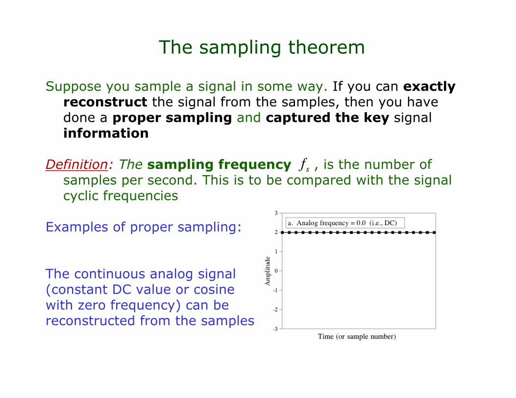
Suppose you sample a signal in some way. If you can exactlyreconstruct the signal from the samples, then you havedone a proper sampling and captured the key signalinformation
Definition: The sampling frequency , is the number ofsamples per second. This is to be compared with the signalcyclic frequencies
Examples of proper sampling:
The continuous analog signal(constant DC value or cosinewith zero frequency) can bereconstructed from the samples
!
!
fs

The sampling theorem
Example of proper sampling (II):
This is a cycle/secondsinusoid sampled at samples/second.In other words, the wave hasa frequency of 0.09 of the samplingrate:
Equivalently, there are samples taken over acomplete cycle of the sinusoid
These samples represent accurately the sinusoid because there is noother sinusoid that can produce the same samples
!
f = 0.09 " fs = 0.09 "1000
!
1000 /90 =11.1
!
fs =1000
!
f = 90

The sampling theorem
Example of proper sampling (III):
Here,This results into samplesper sine wave cycle. Thesamples are so sparse they don’tappear to follow the analog wave
Strange as it seems, it can be proven that no other sine wave canproduce the same type of samples
Since the samples represent accurately the sinusoid they constitute aproper sampling
!
f = 0.31" fs
!
3.2

The sampling theorem
Example of improper sampling:
Here,This results into samplesper sine wave cycle
Clearly, this is an improper sampling of the signal because anothersine wave can produce the same samples
The original sine misrepresents itself as another sine. Thisphenomenon is called aliasing. (The original sine has hidden itstrue identity!)
!
f = 0.95 " fs
!
1.05

The sampling theorem
Suppose a signal’s highest frequency is (a low-pass or a band-pass signal). Then a propersampling requires a sampling frequency at leastsatisfying
The number is called the Nyquist frequency
The number is called the Nyquist rate
Example: Consider an analog signal with frequencies between 0and 3kHz. A proper sampling requires a 6kHZ samplingfrequency or higher
Effects of aliasing: It can change the signal real frequency andthe signal real phase (as we saw in previous slide)
!
fm <f s
2= 0.5 " f s
!
fs
!
fm
!
fs
2
!
2 fm

Discrete-time Signals
Continuous-time signal Discrete-time signalmath: real function of math: sequence
Impulse-sampled signalmath: train of impulses
t
t0 T 2T 3T 4T 5T 6T 7T-T-2T
0 1 2 3 4 5 6 7-1-2 n
!
x" (t) = x(t) "(t # nT)n=#$
$
%
= x[n]"(t # nT)n=#$
$
%
!
x(t)
!
xn
!
t
!
x" (t)
!
x" (t)
!
x(t)
!
x[n] = x(nT)

Sampling in the Frequency Domain
A train of impulses has Fourier Transform
So sampling a continuous-time signal in the time domain
is a convolution in the frequency domain
!
"Ts (t) = "(t # nTs)n=#$
$
% & ' ( ") s( j) ) =
2*
T" j ) # k) s( )( ), ) s =
2*
Tsk=#$
$
%
!
X" ( j# ) =1
2$X j # %&( )( )
%'
'
( "# sj&( ) d&
=1
TsX j # % k# s( )( )
k=%'
'
)!
x" (t) = x(t)"Ts
(t) = x(nTs)
n=#$
n=$
% "(t # nTs)

Sampling in the Frequency Domain
Graphical interpretation of the formula
Continuous-time spectrum
is scaled and replicated (replicas are called aliases)
Aliasing: If signal bandwith then spectrum overlaps!
ω
ωωs 2ωs−ωs 0
!
X" ( j# ) =1
TsX j # $ k# s( )( ),
k=$%
%
& # s = 2' f s, fs =1
Ts
!
fB "f s
2
!
X" ( j# )!
X( j" )

Reconstruction from sampled signal
Question: When can we reconstruct from ?
Answer: If (no aliasing) use a low-pass filter!!
x(t)
!
x"(t)
!
fB <f s
2
ωHlp(ω)
ω
ωωs 2ωs−ωs 0
If (with aliasing) original signal has been lost!
!
fB "f s
2
!
X" ( j# )
!
X( j" )

Aliasing in the frequency domain
In order to understand better why aliasing is produced, and todemonstrate the sampling theorem, let us look at the signalsin the frequency domain
Here the analog signal has a frequency of
!
0.33 " fs < 0.5 " f s

Aliasing in the frequency domain
The sampling of the signal corresponds to doing a convolutionof the signal with a delta impulse train. We call theresulting signal impulse train. The magnitude of thisimpulse train is shown on the right
As you can see, the sampling has the effect of duplicating thespectrum of the original signal an infinite number of times.In other words, sampling introduces new frequencies

Aliasing in the frequency domain
Compare the previous plot with the following one for a differentsampling:
Here, , so this is an impropersampling. In the FD this means that the repeated spectraoverlap. Since there is no way to separate the overlap, thesignal information is lost
!
f = 0.66 " fs > 0.5 " f s

Example
At what rate should we sample the following signal to beable to perfectly reconstruct it?
!
x(t) = 32sinc(101t)cos(200"t)
Go to the frequency domain
!
X( f ) = 32 "101" rect(f
101) *
1
2#( f $100) +#( f +100)( )
=16 "101" rect(f $100
101) + rect(
f +100
101)
%
& '
(
) *
!
Hence fm = 301/2Hz
!
Nyquist rate is 2 fm = 301Hz

Sampling must be done above the Nyquist rate
Cosine sampled at twice itsNyquist rate. Samples uniquelydetermine the signal.
Cosine sampled at exactly itsNyquist rate. Samples do notuniquely determine the signal.
A different sinusoid of the samefrequency with exactly thesame samples as above.

Sampling a Sinusoid
Sine sampled at its Nyquistrate. All the samples are zero.
Adding a sine at theNyquist frequency(half the Nyquistrate) to any signaldoes not change thesamples.

Bandlimited Periodic Signals
If a signal is bandlimited it can be properly sampled accordingto the sampling theorem.
If that signal is also periodic its CTFT consists only of impulses.
Since it is bandlimited, there is a finite number of (non-zero)impulses.
Therefore the signal can be exactly represented by a finite setof numbers, the impulse strengths.

Bandlimited Periodic Signals
If a bandlimited periodic signal is sampled above the Nyquistrate over exactly one fundamental period, that set ofnumbers is sufficient to completely describe it
If the sampling continued, these same samples would berepeated in every fundamental period
So a finite sequence of numbers is needed to completelydescribe the signal in both time and frequency domains

ADC and DAC
GoalsI. From analog signals to digital signals (ADC)
- The sampling theorem
- Signal quantization and dithering
II. From digital signals to analog signals (DAC)
- Signal reconstruction from sampled data
III. DFT and FFT
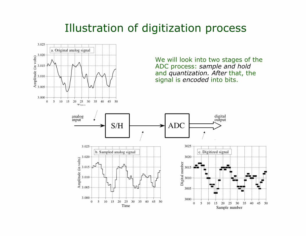
Illustration of digitization process
We will look into two stages of theADC process: sample and holdand quantization. After that, thesignal is encoded into bits.

Digitization process
Sample and hold:The output only changes at periodic instants of time. Theindependent variable now takes values in a discrete set
Before: After sampling:
!
t " {0,0.1,...50},
!
yA (t)" (3000,3025),
!
t " (0,50),
!
yS (t)" (3000,3025),

Digitization process
Quantization:Each flat region in the sampled signal is “rounded-off” to thenearest member of a set of discrete values (e.g., nearest integer)
Before: After quantization:
The quantized signal can be then encoded into bits. A bit is abinary digit (0 or 1). A total of characters (letters of thealphabet, numbers 0 to 9, and some punctuation characters) can beencoded into a sequence of binary bits
!
yQ (t)" {3000,3001,....,3025}
!
t " {0,0.1,...50},
!
t " {0,0.1,...50},
!
yA (t)" (3000,3025),
!
27
=128
!
7
Digitization process
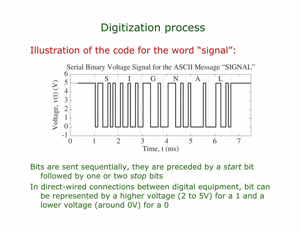
Illustration of the code for the word “signal”:
Bits are sent sequentially, they are preceded by a start bitfollowed by one or two stop bits
In direct-wired connections between digital equipment, bit canbe represented by a higher voltage (2 to 5V) for a 1 and alower voltage (around 0V) for a 0
Signal quantization
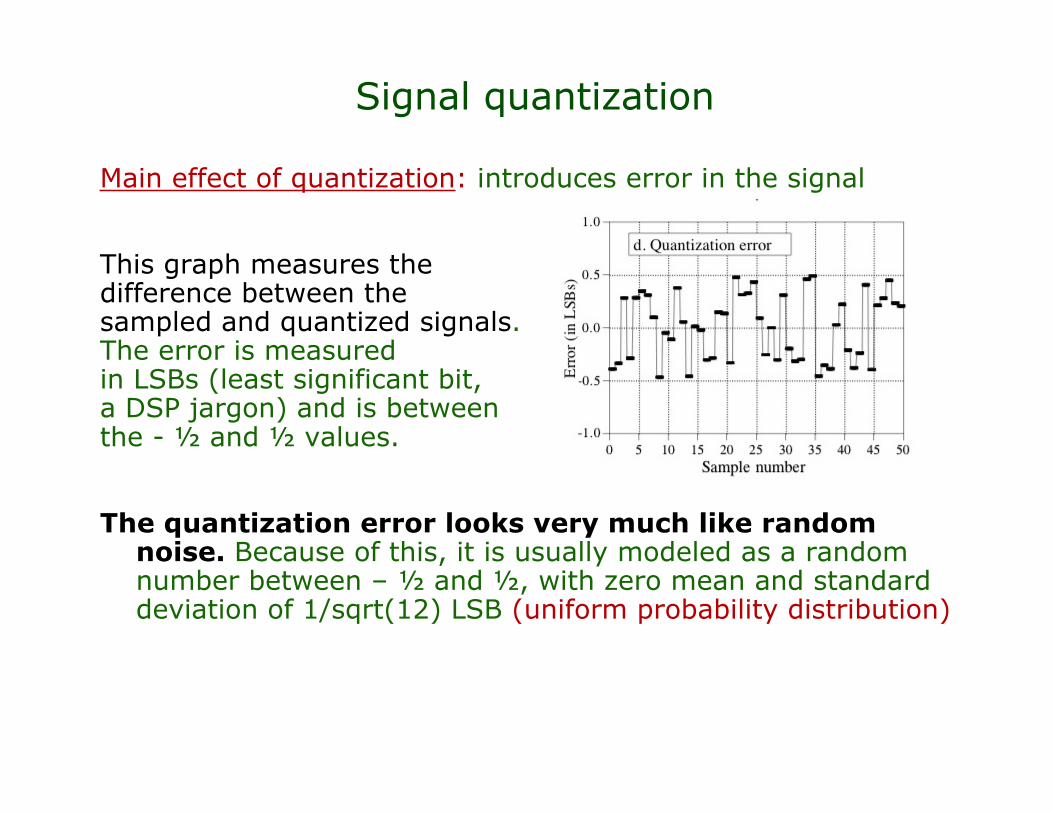
Main effect of quantization: introduces error in the signal
This graph measures thedifference between thesampled and quantized signals.The error is measuredin LSBs (least significant bit,a DSP jargon) and is betweenthe - ½ and ½ values.
The quantization error looks very much like randomnoise. Because of this, it is usually modeled as a randomnumber between – ½ and ½, with zero mean and standarddeviation of 1/sqrt(12) LSB (uniform probability distribution)
!
Signal quantization
Facts:
(1) The random noise or quantization error will add to whatevernoise is present in the analog signal
(2) The quantization error is determined by the number of bitsthat are later used to encode the signal. If we increase thenumber of bits, the error will decrease
Question: How many bits do we need in the ADC? How fineshould the quantization be? (equivalent questions)
Answer: the number of bits chosen should be enough so thatthe quantization error is small in comparison with the noisepresent in the signal
!
Dithering
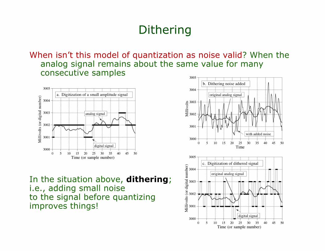
When isn’t this model of quantization as noise valid? When theanalog signal remains about the same value for manyconsecutive samples
In the situation above, dithering;i.e., adding small noiseto the signal before quantizingimproves things!
!

ADC and DAC
GoalsI. From analog signals to digital signals (ADC)
- The sampling theorem
- Signal quantization and dithering
II. From digital signals to analog signals (DAC)
- Signal reconstruction from sampled data
III. DFT and FFT

Digital-to-analog conversion
The DAC reverses the ADC process:(1) It decodes the signal making a conversion from a bit
sequence to an impulse train:

Digital-to-analog conversion
(2) The signal is reconstructed with an electronic low-pass filterto remove the frequencies about ½ the sampling rate
After filtering the impulse train with a such a low pass filter, wewould obtain:

Digital-to-analog conversion
However, the ideal operation just described assumes availabilityof infinitely many samples - not realistic!
Practical operation uses only a finite number of samples. Manytechniques can be used to approximately reconstruct thesignal.
One such technique is a zero-order holder.
Modulated impulses After Zero-Order Holder
t0 T 2T 3T 4T 5T 6T 7T-T-2T!
x" (t)
t0 T 2T 3T 4T 5T 6T 7T-T-2T!
xs(t)

Sampling with Zero-order Holder
A zero-order holder has impulse response
In the frequency domain
0 T t t0 T
ZOH
!
"(t)
!
h(t)
!
H( f ) = F rectt "Ts /2
Ts
#
$ %
&
' (
) * +
, - .
= e" j/ f Ts sinc f Ts( )

Sampling with Zero-order Holder
A sampled signal through a zero-order holder
In the frequency domain
ZOH
!
Xs( f ) = F x" (t)# rectt $Ts /2
Ts
%
& '
(
) *
+ , -
. / 0
=e$ j1 f Ts sinc f Ts( )
TsX( f $ n fs)
k=$2
2
3
t0 T 2T 3T 4T-T-2T!
x" (t)
t0 T 2T 3T 4T-T-2T!
xs(t)

Sampling with Zero-order Holder
In the frequency domain, the zero-order holdertranslates into a multiplication of the real signalspectrum by a sinc function!

Digital-to-analog conversion
In this case you can do several things:
(1) Ignore the effect of the zeroth-order hold and accept theconsequences
(2) Design an analog filter to remove the sinc effect. Forexample an ideal filter that works has this shape:
This will boost the frequenciesthat have been affected bythe sinc function
Other more sophisticatedpossibilities are:(3) Use a fancy “multirate filter” (downsampling, upsampling)(4) Correct for the zeroth order hold before the DAC
Connection to electronic filters
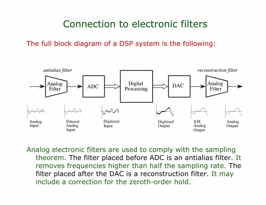
The full block diagram of a DSP system is the following:
Analog electronic filters are used to comply with the samplingtheorem. The filter placed before ADC is an antialias filter. Itremoves frequencies higher than half the sampling rate. Thefilter placed after the DAC is a reconstruction filter. It mayinclude a correction for the zeroth-order hold.

Filters for data conversion
Problem with this design:
Analog filters are not ideal! Thus, knowledge of lowpass filters isimportant to be able to deal with different types of signals(analog filters are being substituted by digital ones)
The filters you choose depend on the application!

ADC and DAC
GoalsI. From analog signals to digital signals (ADC)
- The sampling theorem
- Signal quantization and dithering
II. From digital signals to analog signals (DAC)
- Signal reconstruction from sampled data
III. DFT and FFT
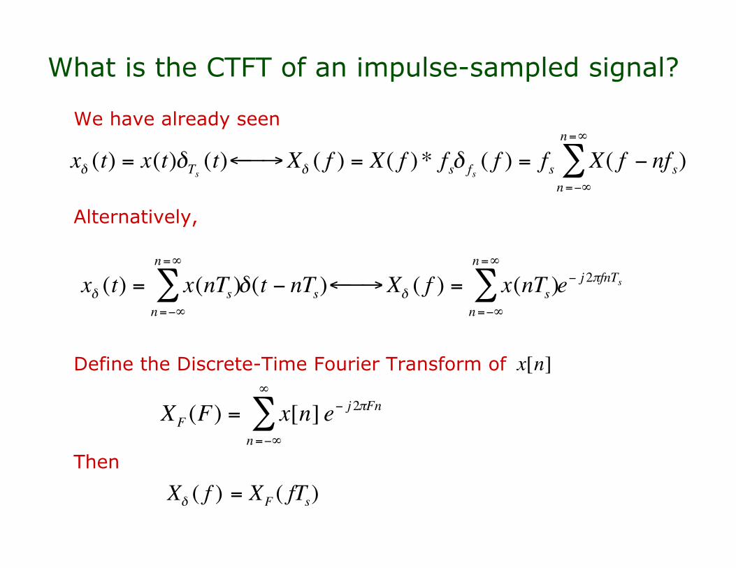
What is the CTFT of an impulse-sampled signal?
We have already seen
Alternatively,
Define the Discrete-Time Fourier Transform of
Then
!
x" (t) = x(t)"Ts (t)# $ % X" ( f ) = X( f ) * f s" fs( f ) = f s X( f & nfs)
n=&'
n='
(
!
XF (F) = x[n]n="#
#
$ e" j 2%Fn
!
x[n]
!
X" ( f ) = XF ( fTs)
!
x" (t) = x(nTs)n=#$
n=$
% "(t # nTs)& ' ( X" ( f ) = x(nTs)n=#$
n=$
% e# j 2)fnTs
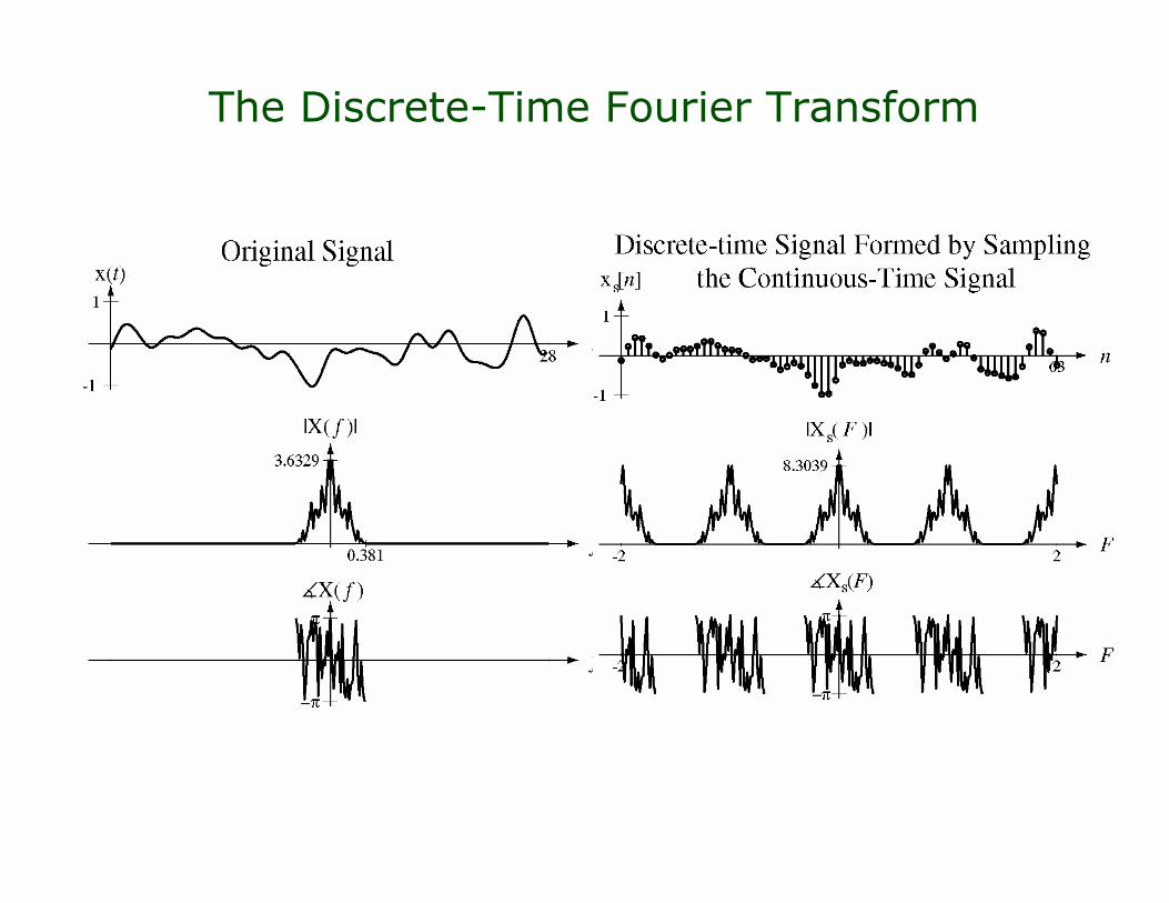
The Discrete-Time Fourier Transform

The Discrete-Time Fourier Series
The Discrete-Time Fourier Transform of discrete-time signal is
is periodic in
The Discrete-Time Fourier Series of periodic discrete-time signal of period is ( )
The DTFT of a periodicsignal is the DTFS:
!
X(F) = x[n]n="#
#
$ e" j 2%Fn& ' ( x[n] = X(F)e
j 2%FndF
0
1
)
!
X(F)!
x[n]
!
F " (0,1]
!
X[k] =1
NF
x[n]k=<NF >
" e# j 2$
nk
NF % & ' x[n] = X[k]ej 2$
nk
NF
k=<NF >
"!
x[n]
!
N0
!
NF
= mN0
!
X(F) = X[k]k="#
k=#
$ %(F " k /N0)

The Discrete Fourier Transform (DFT)
Instead of the DTFS, Matlab implements the DiscreteFourier Transform,
x n[ ] =1
NF
X k[ ]ej2!
nk
NF
k=0
NF "1
# D F T$ %&& X k[ ] = x n[ ]e" j2!
nk
NF
n=0
NF "1
#
which is almost identical to the DTFS
x n[ ] = X k[ ]ej2!
nk
NF
k=0
NF "1
# F S$ %&& X k[ ] =1
NF
x n[ ]e" j2!
nk
NF
n=0
NF "1
#
The difference is only a scaling factor
Two different names for essentially the same object because of historical reasons.

Computing the DFT
One could write a Matlab program to compute the DFT like this..% (Acquire the input data in an array x with NF elements.)..%% Initialize the DFT array to a column vector of zeros.%X = zeros(NF,1) ;%% Compute the Xn’s in a nested, double for loop.%for k = 0:NF-1
for n = 0:NF-1X(k+1) = X(k+1)+x(n+1)*exp(-j*2*pi*n*k/NF) ;
endend..
Quadratic in . Instead, the fast Fourier transform (matlabcommand fft) is an efficient algorithm for computing the DFT.
!
NF

Fast Fourier Transform (FFT)
The algorithm FFT can compute the DFT in operations
The FFT takes an N-sample time-sequence {xn}And gives us an N-sample frequency-sequence {Xk}
This is reversible via the IFFT operationNo data is lost in either direction
Recall periodicity of DFT
The FFT describes the signal in terms of its frequency contentIf we sampled fast enough, this is the same as the Fourier
Transform of the original continuous-time signal
The FFT is a primary tool for data analysis
!
X[k + NF] = X[k]
!
O(NFlog2 NF
)

Speed comparison DFT/FFTBelow is a speed comparison for various numbers of samples (N).(A means # additions and M means # multiplications.)
! N = 2!
ADFT
MDFT
AFFT
MFFT
ADFT/ A
FFTM
DFT/ M
FFT
1 2 2 4 2 1 1 4
2 4 12 16 8 4 1.5 4
3 8 56 64 24 12 2.33 5.33
4 16 240 256 64 32 3.75 8
5 32 992 1024 160 80 6.2 12.8
6 64 4032 4096 384 192 10.5 21.3
7 128 16256 16384 896 448 18.1 36.6
8 256 65280 65536 2048 1024 31.9 64
9 512 261632 262144 4608 2304 56.8 113.8
10 1024 1047552 1048576 10240 5120 102.3 204.8

The z-Transform
What is the Laplace transform of a sampled signal?
where
is the z-Transform. The inverse formula is a bit more involvedbut often not needed!
Generalizes the DTFT. Surprised?
!
Xs(s) = x(t) "
T(t) e
#stdt
0
$
%
= x(t) "(t # nT)n=#$
$
& e#stdt
0
$
% = x(nT)e#snT
n= 0
$
&
= X(esT)
!
X(z) = xn
n= 0
"
# z$n

Discrete-time Systems with the z-Transform
Some properties of the z-Transform
(integration in Laplace)
(differentiation in Laplace)
(convolution)
Proofs are easier, e.g.
!
Z xn"1{ } = z"1 Z x
n{ }
!
Z xn+1{ } = z Z x
n{ }" x0( )
!
Z xn " yn{ } = Z xn{ }Z yn{ }
!
Z xn"1{ } = z
"1xk"1z
"k
k=1
#
$%
& '
(
) * z = z"1 x
k"1z"(k"1)
k=1
#
$ = z"1 xnz"n
n= 0
#
$ = z"1Z xn{ }

Discrete-time Systems with the z-Transform
We use the basic property(integration in Laplace)
to study the system described by the lineardifference equation
as with Laplace trasforms we have
from where we obtain the transfer function
!
Z xn"1{ } = z"1 Z x
n{ }
!
yn "# yn"1 = xn
!
Y (z) "# z"1Y (z) = X(z)
!
Y (z) = H(z)X(z)
!
H(z) =z
z "#=
1
1"#z"1

Discrete-time Systems with the z-Transform
When is a pulse ( )
and
from where we compute the impulse response
!
X(z) = Z xn{ } = Z "
n{ } =1
!
hn
= Z"1H(z){ } =# n
!
Y (z) = H(z) =1
1"# z"1=1+# z"1 + # 2
z"2
+# 3z"3
+L = #nz"n
n= 0
$
%
!
xn
= "n
!
"0
=1, "k
= 0, k # 0
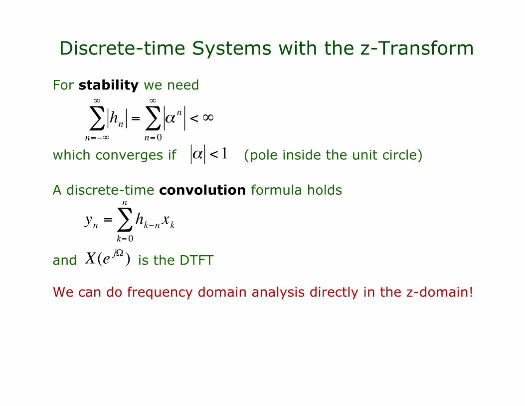
Discrete-time Systems with the z-Transform
For stability we need
which converges if (pole inside the unit circle)
A discrete-time convolution formula holds
and is the DTFT
We can do frequency domain analysis directly in the z-domain!
!
hn
n="#
#
$ = % n
n= 0
#
$ <#
!
" <1
!
yn = hk"n xkk= 0
n
#
!
X(ej")
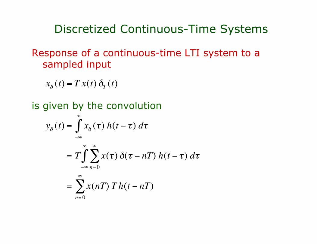
Discretized Continuous-Time Systems
Response of a continuous-time LTI system to asampled input
is given by the convolution
!
x" (t) = T x(t) "T(t)
!
y" (t) = x" (#) h(t $ # ) d#$%
%
&
= T x(# )n= 0
%
' "(# $ nT) h(t $ # ) d#$%
%
&
= x(nT)n= 0
%
' T h(t $ nT)
Discretized Continuous-Time Systems
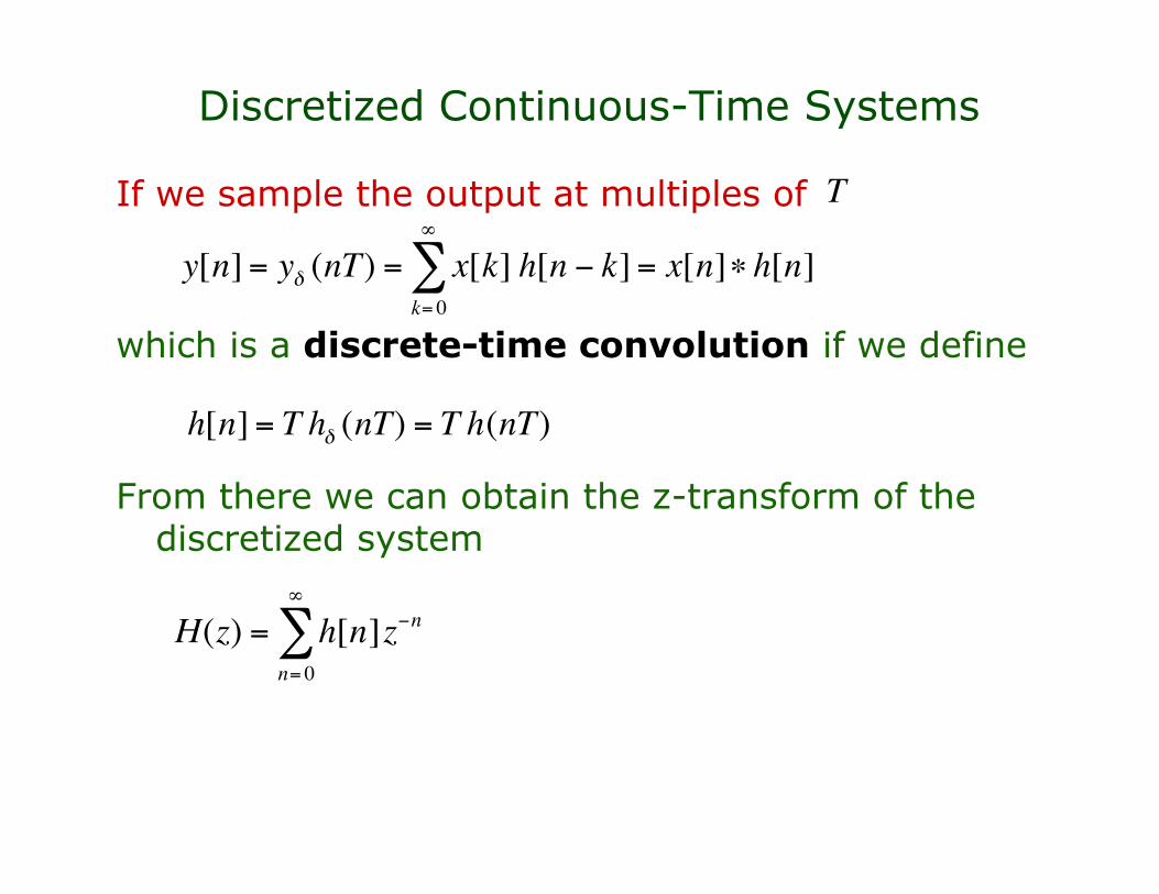
If we sample the output at multiples of
which is a discrete-time convolution if we define
From there we can obtain the z-transform of thediscretized system
!
y[n] = y" (nT) = x[k]k= 0
#
$ h[n % k] = x[n]& h[n]
!
h[n] = T h" (nT) = T h(nT)
!
H(z) = h[n]z"n
n= 0
#
$
!
T

Discretized Continuous-Time Systems
For example
we have
Continuous-time pole becomes !
!
h(t) = be"atu(t)
!
H(z) = Tbe"a nT
z"n
n= 0
#
$ = Tb e"aT( ) n
z"n
n= 0
#
$ =Tb
1" e"aT z"1
=Tbz
z " e"aT
!
H(s) =b
s+ a
!
s = "a
!
z = e"aT


![DAC&ADC [EngineeringDuniya.com]](https://static.documents.pub/doc/80x56/577cdcbb1a28ab9e78ab41f0/dacadc-engineeringduniyacom.jpg)


