38


SAND97-2019Unlimited Release
Printed August 1997
A Multi-Level Code for Metallurgical Effects inMetal-Forming Processes
Paul A. Taylor and Stewart A. SillingComputational Physics and Mechanics Department
Sandia National LaboratoriesP.O. Box 5800
Albuquerque, NM 87185-0820
Darcy A. HughesMaterials Reliability Department
Douglas J. Bammann and Michael L. ChiesaSolid and Material Mechanics Department
Sandia National LaboratoriesP.O. Box 969
Livermore, CA 94551-0969
Abstract
We present the final report on a Laboratory-Directed Research and Develop-ment (LDRD) project,A Multi-Level Code for Metallurgical Effects in Metal-Forming Processes, performed during the fiscal years 1995 and 1996. Theproject focused on the development of new modeling capabilities for simulat-ing forging and extrusion processes that typically display phenomenology oc-curring on two different length scales. In support of model fitting and codevalidation, ring compression and extrusion experiments were performed on304L stainless steel, a material of interest in DOE nuclear weapons applica-tions.
DistributionCategory UC-705
3

4
Acknowledgments
The authors would like to thank the following people: Mr. R.Bell for the development and implementation of the movingsubgrid scheme, Mr. J. Totten for his execution of the ringcompression experiments, Mr. N. Bhathena, of Wyman-Gordon Forgings, in conducting the extrusion experiments,Mr. H. Hsiung for his assistance in the metallurgical analysisof the extrusion samples, and Ms. M. Chen for her assistancein data digitizing and image scanning.

5
Contents
1. Introduction............................................................................................................ 72. Computer Code Enhancements.............................................................................. 9
2.1. Multi-Grid Scheme in CTH/EPIC ................................................................ 92.2. Dynamic Relaxation Algorithm.................................................................... 102.3. Viscoplasticity Constitutive Model .............................................................. 102.4. Friction Model .............................................................................................. 12
3. Experimental Results ............................................................................................. 133.1. Ring Compression Experiments ................................................................... 133.2. Extrusion Experiments.................................................................................. 15
4. Fitting and Validation ............................................................................................ 214.1. Friction Model Fitting................................................................................... 214.2. Code Validation ............................................................................................ 21
5. Summary................................................................................................................ 23References.................................................................................................................. 25Appendix A. Moving Subgrid Option ....................................................................... 27Appendix B. Dynamic Relaxation Algorithm ........................................................... 29
B.1. DR for Equilibrium Problems ...................................................................... 29B.2. DR for Quasi-static Problems ...................................................................... 30B.3. Application of Loads.................................................................................... 33B.4. Convergence Test......................................................................................... 33B.5. Choice of Damping Coefficient ................................................................... 34B.6. Constitutive Modeling Issues....................................................................... 35B.7. Code Modification Steps.............................................................................. 35
Figures
2.1. Eulerian/Lagrangian description of forging problem with Eulerian subgrids .... 92.2. (a)-Initial configuration and (b)-equivalent plastic strain plot at 7 sec. into extrusion simulation using CTH/EPIC and the dynamic relaxation technique .. 112.3. Graphic description of Anand’s friction model for metal-forming .................... 123.1. Schematic of ring compression experiment........................................................ 133.2. Ring compression data for 304L stainless steel at 800oC................................... 143.3. Ring compression data for 304L stainless steel at 1000oC................................. 143.4. Schematic diagram of the extrusion experiments ............................................... 153.5. Optical micrograph and corresponding plastic shear strain distribution for upper section of extrusion specimen 1 (specimen radius ~ 3.1 mm)................... 173.6. Optical micrograph and corresponding plastic shear strain distribution for middle section of extrusion specimen 1 (specimen radius ~ 3.1 mm)................. 183.7. Optical micrograph and corresponding plastic shear strain distribution for lower section of extrusion specimen 1 (specimen radius ~ 3.1 mm)................... 19A.1. Graphical representation of moving subgrid option .......................................... 27B.1. Solution of an equilibrium problem by DR. Time evolutions of the load and the total kinetic energy of the mesh are shown................................................... 31

6
B.2. Solution of a quasi-static problem by DR .......................................................... 32

7
Introduction
1. Introduction
This report summarizes the work performed for the Laboratory-Directed Research andDevelopment (LDRD) project,A Multi-Level Code for Metallurgical Effects in Metal-Forming Processes.
The objective of this project was the development of a multi-level computational methodto predict the final thermomechanical state of a material that has undergone a forging orextrusion process. Typically, in such a process, there exist localized regions, or “boundarylayers,” of the workpiece that are in close proximity to the tooling hardware and, as aconsequence, experience significantly greater temperature gradients and strains thanmaterial somewhat removed from the workpiece/tooling interface. Therefore, thesimulation method must be able to predict both (1) the overall bulk flow of the workpiecematerial and (2) the microscale effects that occur in the boundary layer of the workpiecenear the interface between it and the tooling hardware.
In order to accurately simulate forging and extrusion processes, we have developed a multi-grid method that would predict and couple the thermomechanical responses of theworkpiece in two distinct length-scale regimes: the bulk flow regime, and the boundarylayer regime in which the characteristic length scale can be on the order of 1/10 to 1/100of that characteristic of the bulk flow regime. This scheme was incorporated into a coupledEulerian/Lagrangian code in which the workpiece response could be modeled in anEulerian grid and the tooling hardware modeled using Lagrangian finite element methods.Eulerian grid subdomains of high resolution are used to model the phenomena occurring inthe boundary layer of the workpiece, the solution of which is then coupled to the hybridEulerian/Lagrangian calculation to predict the overall material flow of the workpiece.
The codes chosen for the Eulerian/Lagrangian coupling are the solid dynamics codes, CTH[1] and EPIC [2]. The linking of CTH and EPIC is accomplished using the driver code,Zapotec [3]. Zapotec employs a hybrid Eulerian/Lagrangian solution methodology [4] inwhich soft material is treated in an Eulerian framework and hard material is modeled witha Lagrangian code.
The solid dynamics code CTH is an Eulerian code that explicitly solves the finite-difference analogs for the equations of momentum and energy balance; whereas, EPIC is aLagrangian finite element code that also employs an explicit time integration scheme tosolve the equations of momentum and energy balance. As such, both of these codes employthe Courant criterion that restricts the size of the time step taken at each iteration to ensurethe stability of their numerical solutions. This feature in the codes imposes a significantrestriction on the applicability of the CTH/EPIC coupled code to problems of forging andextrusion. In particular, the CTH/EPIC coupled code with its explicit time integrationschemes is well suited to treating solid dynamics problems that occur on microsecond tomillisecond time scales whereas, forging and extrusion processes typically occur on a timescale of 0.1 to 10 seconds. Early attempts to use CTH/EPIC to simulate a forging orextrusion process required simulation times on the order of a hundred microseconds, whichgave rise to unacceptable consequences due to material inertia and strain rate effects.

8
Consequently, another aspect of the LDRD project was the development andimplementation of a time integration scheme based on the dynamic relaxation method [5].This approach allows us to avoid the adverse consequences of the timestep constraintsinherent in CTH and EPIC and permits the simulation of quasi-static processes such asforging and extrusion.
In order to represent the complex temperature-dependent plastic flow of the workpiece, asophisticated viscoplasticity model is required. Consequently, another task of the LDRDproject was the implementation and testing of the Bammann-Chiesa-Johnson (BCJ)viscoplastic/damage model [6,7]. This model describes the deviatoric elastic-viscoplasticresponse of metals at temperatures below melt and the cumulative damage resulting fromductile void growth.
Representation of the friction forces between the workpiece and the tooling hardwarerequired us to adopt an accurate friction model relevant to metal forming applications. Inparticular, the friction model developed by Anand and Tong [8] was implemented into theCTH/EPIC code and fitted to ring compression data collected for the project.
For the purposes of model fitting and code validation, we selected 304L stainless steel as acandidate material which is of particular interest in DOE nuclear weapons applications. Inorder to fit the friction model implemented for the project, we conducted ring compressionexperiments on 304L stainless steel at the elevated temperatures typical of forging andextrusion operations for this material. For the purpose of validating our simulation method,we also conducted extrusion experiments and subsequent metallurgical analyses onsamples of 304L stainless steel to determine the resulting internal plastic flow field of thesamples. Validation then becomes a matter of comparing the experimentally determinedplastic flow field, as induced by the extrusion process, and its prediction by means ofnumerical simulation.

9
Computer Code Enhancements
2. Computer Code Enhancements
2.1 Multi-Grid Scheme in CTH/EPIC
In general, forging and extrusion problems involve soft and hard materials (viz., workpieceand tooling hardware), interacting with each other. The workpiece material tends toundergo large strains; whereas, the tooling hardware experiences small strains and usuallyremains elastic in its response. The application of Eulerian/Lagrangian methods to forging/extrusion problems brings with it two distinct advantages over strictly Eulerian orLagrangian methods. First, the Eulerian portion can track the flow of the workpiece withoutconcern for mesh entanglement, and the Lagrangian finite element representation of thetooling hardware provides a fast calculation of its material response. Secondly, byoverlaying the Eulerian mesh to include the tooling hardware boundaries, we have a well-defined interface at which friction and heat transfer models can be applied.
In many forging/extrusion applications, the friction and heat transfer that occur at theinterfaces between the workpiece and tooling hardware give rise to significantly greaterplastic strains and temperature gradients in a “boundary layer” located within theworkpiece adjacent to the material interface. In order to efficiently resolve the phenomenaoccurring in the boundary layer, we have developed a multi-grid scheme that overlays anEulerian subgrid of much finer resolution than that which tracks the bulk response of theworkpiece material (see Figure 2.1). By defining mesh cell dimensions of much finer sizein the subgrids, we can model the thermomechanical response of the workpiece in theboundary layer with greater resolution.
Figure 2.1. Eulerian/Lagrangian description of forging problem with Eulerian subgrids.
In order to be useful, the Eulerian subgrids must be able to move along with and track thematerial interfaces. This is achieved by identifying each subgrid with a Lagrangian tracerpoint, i.e., a point that is originally fixed in one of the materials in close proximity to the
Lagrangian
EulerianLagrangian
Subgrids
WorkpieceDie
LagrangianPunch

10
interface and moves along with that material. Further details of this scheme as it isimplemented in CTH can be found in Appendix A.
2.2 Dynamic Relaxation Algorithm
The codes selected for our Eulerian/Lagrangian methodology are the Eulerian finitedifference code CTH [1] and the Lagrangian finite element code, EPIC [2]. As mentionedpreviously, these codes are well suited to solving various solid dynamics problems andwere not originally intended to simulate low strain-rate processes. Since the majority offorging and extrusion processes involve low strain-rates, we needed to implement a timeintegration scheme in CTH and EPIC that would relax the time step controls used by thecodes so that these processes could be simulated. The scheme we adopted is based on thedynamic relaxation (DR) technique [5] which is used with solid dynamics codes to solveequilibrium or quasi-static problems in continuum and structural mechanics. The specificson the technique and its implementation into solid dynamics computer codes is outlined ingreater detail in Appendix B.
A sample extrusion simulation, represented in Figure 2.2, demonstrates the CTH/EPICcoupled code employing the dynamic relaxation algorithm. In the figure, the extrusionpunch and die are represented by the finite element meshes and the workpiece billet isextruded partially through the die over a period of 7 seconds. The problem geometry isaxisymmetric (about the X=0 axis) with the tooling hardware modeled as S-7 tool steel and
the workpiece as copper at 800oC. The figure displays only half of the tooling hardwarewhereas the workpiece is fully shown. In Figure 2.2b, the apparent “liner” around theworkpiece is an artifact of the graphics software displaying the problem and the coupledEulerian/Lagrangian methodology of the Zapotec code.
2.3 Viscoplasticity Constitutive Model
During a forging or extrusion process, the workpiece can undergo a complex history ofdeformation at elevated temperatures. Typically, the response of the workpiece materialwill be a result of strain hardening, strain rate effects, and thermal softening. The strainhardening can be due to a combination of isotropic and kinematic hardening. Consequently,the need exists for an advanced plasticity model that can capture these effects if one hopesto accurately simulate forging and extrusion processes.
We have implemented the Bammann-Chiesa-Johnson (BCJ) [6,7] viscoplastic/damagemodel into the CTH/EPIC code to describe the response of the workpiece material. Inparticular, the model describes the deviatoric elastic-viscoplastic response of metals and thecumulative damage resulting from ductile void growth. The viscoplastic response of themodel incorporates isotropic and kinematic hardening as well as strain rate and thermaleffects. Damage modeling is based on an analytic expression for spherical void growth. Thedamage growth rate is dependent on the effective stress, tensile pressure, plastic strain rate,and the current damage level. The deviatoric response of the model is dependent on thedamage in such a way as to locally degrade elastic moduli and concentrate plastic flow. A

11
Computer Code Enhancements
complete description of the BCJ model, its implementation into the code, and a simulationexemplifying the model is described in a separate Sandia report [9].
Figure 2.2. (a)-Initial configuration and (b)-equivalent plastic strain plot at 7 secondsinto extrusion simulation using CTH/EPIC and the dynamic relaxation technique.
Time = 0(a)
Punch
Die
Workpiece
Temperature = 800oC
Time = 7 sec.
Equivalent Plastic Strain of Workpiece
(b)

12
2.4 Friction Model
In order to describe the friction forces that exist at the interface between the workpiecematerial and tooling hardware, we have implemented an advanced friction model that hasbeen proposed by Anand and Tong [8] specifically for metal-forming applications. Thefriction model defines the relation between the resultant shear stress at a material
interface and its associated normal stress resultant according to the relation
, (2.1)
where is the asymptotic value of for large values of , and is the coefficient of
friction for low values of . A graphical description of the friction model is depicted inFigure 2.3.
Figure 2.3. Graphic description of Anand’s friction model for metal-forming.
The friction model is implemented in the Zapotec [3] driver code that couples CTH andEPIC to treat solid dynamics problems using the hybrid Eulerian/Lagrangian solutionmethodology.
τσ
τ τ∞ µσ
τ∞-------
tanh=
τ∞ τ σ µσ
µσ
τ
τ∞

13
Experimental Results
3. Experimental Results
3.1 Ring Compression Experiments
This section describes the ring compression experiments that were conducted at elevatedtemperatures in order to fit the friction model (see e.g., [10]), outlined in section 2.4, todescribe the interfacial stresses that will be encountered in the extrusion experiments on304L stainless steel. Ring compression tests are typically performed in order to determinethe interfacial friction stresses that exist between the ring specimen and the toolinghardware, or platens, that compress the specimen axially to a predetermined extent (seeFigure 3.1). The amount of friction that exists between the ring specimen and the platens isreflected by the extent of change in the inside diameter of the ring. (Little or no frictionresults in an increase of the inside diameter during compression, whereas a large amount offriction results in a decrease of the inside diameter). For model fitting purposes, useful ringcompression data typically assumes the form of “decrease in inner diameter” as a functionof “reduction in thickness.”
Figure 3.1. Schematic of ring compression experiment.
Ring compression experiments and the resulting friction data can be obtained for either dryor lubricated samples. Since the extrusion experiments, performed for code validationpurposes and described in section 3.2, involve lubrication, we have conducted our ringcompression experiments using the same lubricant employed in those extrusions.
In our ring compression experiments, the specimen geometry was that of a hollow circularcylinder (or disk) with an inside diameter of 1.016 cm, an outside diameter of 2.032 cm,and an axial thickness of 0.6782 cm. The samples were placed between flat platens
consisting of either the Inconel X-750 alloy (for experiments at 800oC) or a Si3N4 ceramic
(for experiments at 1000oC).
The ring compression experiments subjected the 304L stainless steel ring samples to axialcompressions of up to roughly a 60% reduction in thickness for two different temperatures,
namely, 800oC and 1000oC. There were 20 ring compression experiments conducted at
800oC and 16 experiments conducted at 1000oC. The experimental results for the ring
Upper Platen
Lower Platen
Ring Specimen
Neutral Surface

14
compression tests at 800oC and 1000oC are presented in Figures 3.2 and 3.3 respectively.The existence of the low data point (at 48% reduction in thickness) in Figure 3.3 can beattributed to the loss of lubrication during the associated experiment. Consequently, thispoint was ignored in the fitting of the friction model as described later in section 4.1.
Figure 3.2. Ring compression data for 304L stainless steel at 800oC.
Figure 3.3. Ring compression data for 304L stainless steel at 1000oC.
0.0
10.0
20.0
30.0
Reduction in Thickness (%)
Dec
reas
e in
Inne
r D
iam
eter
(%
)
0 10 20 30 40 50 60
0.0
10.0
20.0
30.0
40.0
50.0
Reduction in Thickness (%)
Dec
reas
e in
Inne
r D
iam
eter
(%
)
0 10 20 30 40 50 60 70

15
Experimental Results
3.2 Extrusion ExperimentsIn order to validate our simulation method, extrusion experiments were performed on 304Lstainless steel samples containing ferrite stringers. These stringers, initially orientedperpendicular to the longitudinal axis of each specimen, are re-oriented during theextrusion process reflecting the internal plastic flow field of the specimen. Subsequentmetallurgical analyses were performed on sections of the extruded specimens to determinestringer orientations throughout the specimen. Using a simple relation between change instringer orientation and shear strain, we were able to determine the plastic shear straindistributions throughout each specimen.
In the experiments, cylindrical samples of 304L stainless steel were extruded, underisothermal conditions, through a reduction die to 25% of the sample’s original diameter(see Figure 3.4).
Figure 3.4. Schematic diagram of the extrusion experiments.
Top Column
Top Flat Die
Extrusion Punch
Support Die
Extrusion Die
Graphite Plug
Specimen
Base w/Hole
Bottom Columnw/Hole
Through HoleTo Actuator
To Load Cell

16
The extrusion experiments were performed at the Wyman-Gordon Forgings Company,Houston, Texas, under the direction of Mr. Noshir Bhathena. Four extrusions wereconducted for the project; the first three under identical conditions and the fourth at a higherram speed and hence, higher strain rate. The conditions of the experiments were as follows:
Sample composition: 304L stainless steel
Temperature: 1037oC (isothermal conditions: both sample and tooling hardware)
Initial sample geometry: cylindrical, 1.27 cm diameter, 1.27 cm long
Final sample geometry: cylindrical, 0.635 cm diameter, ~5 cm long
Lubricant: glass-based (proprietary information of Wyman-Gordon)
Tooling composition: super alloy (proprietary information of Wyman-Gordon)
Die angle: 60o
Die throat diameter: 0.635 cm
Ram Speed: 0.13 cm/min (experiments 1-3), 1.4 cm/min (experiment 4)
Nominal strain rate: 0.01/sec (experiments 1-3), 0.10/sec (experiment 4)
The shear strain distribution data from the low strain rate experiments 1-3 are fairlyconsistent whereas the data from the higher strain rate experiment 4 is incomplete due tothe lack of ferrite stringer image data in the upper 1/3 of the specimen. However, the straindistribution in the remainder of specimen 4 suggests little difference between the results ofexperiments 1-3 and those of experiment 4, which was conducted at the higher ram speed.
Figures 3.5, 3.6, and 3.7 display the plastic shear strain distributions in the upper, middle,and lower thirds of the extrusion specimen from experiment 1 along with the correspondingoptical micrographs of the specimen’s cross-section. The micrographs were used todetermine the strain distributions by tracking the reorientation of the ferrite stringers, whichappear as dark lines in the micrographs. Note also, the concave shape at the top of the uppersection of the specimen in Figure 3.5. This feature is a result of “suck-in,” a term used inthe forging industry to describe the process of material being drawn in towards the centerof the specimen as a result of extrusion process. Suck-in was observed in all four extrusionexperiments.
Error bars are included in the shear strain distribution plots, which are a result of theuncertainty of measuring the angles through which the ferrite stringers rotated. As can beseen in all three sections, the plastic shear strain increases exponentially from a value ofzero at the center of the specimen to values ranging from 10 to 50 at the maximum radialdistance of the specimen. Furthermore, this radial dependence of the plastic shear strainappears qualitatively similar for all three sections.

17
Experimental Results
Finishing End
Figure 3.5. Optical micrograph and corresponding plastic shear strain distribution for up-per section of extrusion specimen 1 (specimen radius ~ 3.1 mm).
Body
Suck-in
1.0 1.5 2.0 2.5 3.0Radial Distance from Center (mm)
0
10
20
30
40
50
She
ar S
trai
n,γrz

18
Figure 3.6. Optical micrograph and corresponding plastic shear strain distribution formiddle section of extrusion specimen 1 (specimen radius ~ 3.1 mm).
0
10
20
30
40
50
She
ar S
trai
n,
0.0 0.5 1.0 1.5 2.0Radial Distance from Center (mm)
2.5 3.0

19
Experimental Results
Figure 3.7. Optical micrograph and corresponding plastic shear strain distribution forlower section of extrusion specimen 1 (specimen radius ~ 3.1 mm).
Body
Starting End
0
10
20
30
40
50
She
ar S
trai
n,
0.0 0.5 1.0 1.5 2.0Radial Distance from Center (mm)
2.5 3.0

20
Intentionally Left Blank
21
Fitting and Validation
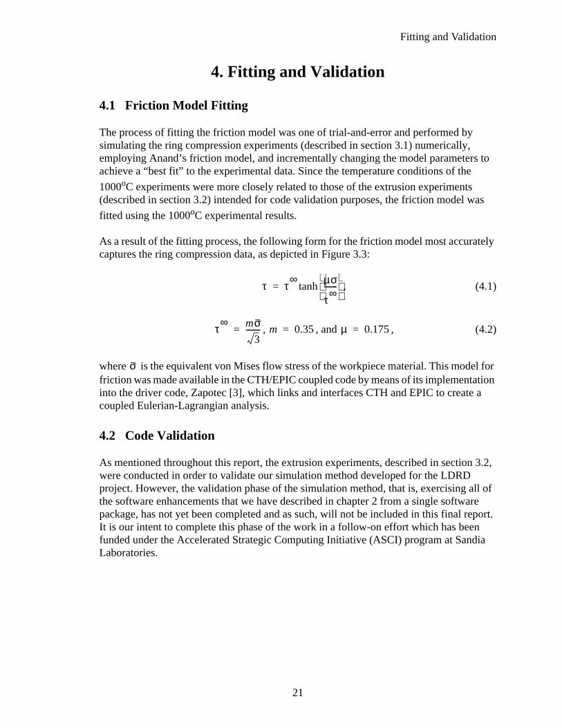
4. Fitting and Validation
4.1 Friction Model Fitting
The process of fitting the friction model was one of trial-and-error and performed bysimulating the ring compression experiments (described in section 3.1) numerically,employing Anand’s friction model, and incrementally changing the model parameters toachieve a “best fit” to the experimental data. Since the temperature conditions of the
1000oC experiments were more closely related to those of the extrusion experiments(described in section 3.2) intended for code validation purposes, the friction model was
fitted using the 1000oC experimental results.
As a result of the fitting process, the following form for the friction model most accuratelycaptures the ring compression data, as depicted in Figure 3.3:
, (4.1)
, , and , (4.2)
where is the equivalent von Mises flow stress of the workpiece material. This model forfriction was made available in the CTH/EPIC coupled code by means of its implementationinto the driver code, Zapotec [3], which links and interfaces CTH and EPIC to create acoupled Eulerian-Lagrangian analysis.
4.2 Code Validation
As mentioned throughout this report, the extrusion experiments, described in section 3.2,were conducted in order to validate our simulation method developed for the LDRDproject. However, the validation phase of the simulation method, that is, exercising all ofthe software enhancements that we have described in chapter 2 from a single softwarepackage, has not yet been completed and as such, will not be included in this final report.It is our intent to complete this phase of the work in a follow-on effort which has beenfunded under the Accelerated Strategic Computing Initiative (ASCI) program at SandiaLaboratories.
τ τ∞ µσ
τ∞-------
tanh=
τ∞ mσ3
--------= m 0.35= µ 0.175=
σ

22
Intentionally Left Blank

23
Summary
5. Summary
In this report, we have described a method that is intended to provide a simulationcapability to accurately model forging and extrusion processes. Typically, these processesinvolve thermomechanical phenomena occurring on multiple length scales. We have useda computational platform that employs a hybrid Eulerian-Lagrangian analysis as thebaseline modeling technique. Several new capabilities were implemented in the baselinesimulation method under this project. In particular, we have implemented:
1. A dynamic relaxation algorithm that permits us to simulate forging and extrusionprocesses on long time scales.
2. A multi-grid scheme to simulate the thermomechanical response of materials ondifferent spatial length scales.
3. The Bammann-Chiesa-Johnson (BCJ) constitutive model describing viscoplasticityand damage accumulation as it occurs in the workpiece material.
4. An advanced friction model specifically designed to describe the interfacial stressesthat exist between the workpiece and tooling hardware.
Furthermore, we have conducted:
5. Ring compression experiments on lubricated samples of 304L stainless steel attemperatures that are typical of forging and extrusion operations for this material.
6. Calibration of the friction model using the ring compression data to define theworkpiece/tooling interactions that will exist in the subsequent extrusion experimentsperformed on 304L stainless steel.
7. Extrusion experiments on samples of 304L stainless steel and subsequentmetallurgical analyses on cross-sections of the extruded samples. From these analyses,we have determined the internal plastic flow fields of the samples that were inducedby the extrusion process. This data is used for validation purposes by comparing theexperimentally determined plastic flow fields, as induced by the extrusion process, andtheir prediction by means of simulation.
The validation phase of the project, however, has not yet been completed and as such, willnot be included in this final report. It is our intent to complete this phase of the work anddocument the results in a forthcoming report. Follow-on funding has been secured for thispurpose.

24
Intentionally Left Blank

25
References
References
[1] J. M. McGlaun, S. L. Thompson, L. N. Kmetyk, and M. G. Elrick, “A Brief Descriptionof the Three-Dimensional Shock Wave Physics Code CTH,” Sandia NationalLaboratories report SAND89-0607 (1990).
[2] G. R. Johnson, R. A. Stryk, T. J. Holmquist, and S. R. Beissel, “User Instructions forthe 1996 Version of the EPIC Code,” Alliant Techsystems Inc., Hopkins, Minnesota,March 1996.
[3] J. K. Prentice, “A Methodology for Performing Coupled Eulerian/Lagrangian SolidDynamics Hydrocode Calculations,” in preparation.
[4] J. K. Prentice, “Methodology and Applications of the Hull Hydrocode Eulerian/Lagrangian Link,” inShock Waves in Condensed Matter-1987, S. C. Schmidt and N. C.Holmes, eds., pp. 219-222, North-Holland Physics Publishing (1988).
[5] P. Underwood, “Dynamic Relaxation,” inComputational Methods for TransientAnalysis, T. Belytschko and T. J. R. Hughes, eds., Elsevier Science Publishers B.V., pp.245-265 (1983).
[6] D. J. Bammann, M. L. Chiesa, M. F. Horstemeyer, and L. I. Weingarten, “Failure inDuctile Materials using Finite Element Methods,” in Structural Crashworthiness andFailure, eds. N. Jones, and T. Wierzbicki, Elsevier Applied Science, 1 (1993).
[7] D. J. Bammann, M. L. Chiesa, A. McDonald, W. A. Kawahara, J. J. Dike, and V. D.Revelli, “Prediction of Ductile Failure in Metal Structures,” in:Failure Criteria andAnalysis in Dynamic Response, ed. H. E. Lindberg, ASME AMD, vol. 107, 7 (1990).
[8] L. Anand and W. Tong, “A Constitutive Model for Friction in Forming,” Annals of theCIRP, vol. 42/1, 361 (1993).
[9] P. A. Taylor, “CTH Reference Manual: The Bammann-Chiesa-Johnson Viscoplastic/Damage Model,” Sandia National Laboratories report SAND96-1626 (1996).
[10] A. T. Male and M. G. Cockcroft, “A Method for the Determination of the Coefficientof Friction of Metals under Conditions of Bulk Plastic Deformation,” J. Inst. Met.93,38 (1964-1965).

26
Intentionally Left Blank

27
Moving Subgrid Option
Appendix A. Moving Subgrid Option
The CTH code has been modified to use separate domains (blocks) for various portions ofa problem domain. This option is known as Multi-Block Communication (MBC). Toincrease the usefulness of this option it has been further modified to allow separate blocksto move relative to the main mesh. To achieve this, each block (a subgrid) is identifiedwith one Lagrangian tracer point (see Figure A.1). As the material moves through the sub-grid the tracer is moved at the material velocity. Once the tracer has moved more than 2cells from its original position (the (I,J,K) position in the subgrid), the block is rezoned toplace the tracer back at the original (I,J,K) site in the subgrid. This effectively causes thesubgrid to move an integer number of cells widths whenever the tracer position exceedsthe trigger criterion. This typically requires several computational cycles since materialmoves less (usually much less) than one cell width per computational cycle. It is importantto note that the rezone step requires significantly more computational time than the usualcycle time, so not doing the rezone every cycle reduces the overall computation time.MBC also does a rezone each cycle, but only for the overlapping zones (where the block toblock communication is accomplished).
Figure A.1. Graphical representation of moving subgrid option.
*
Tracer Position After Rezone
Subgrid Position
Subgrid PositionAfter Rezone
Workpiece Material
New Tracer Position
Original Tracer Position
Tooling Material
*
*
FlowField
FlowField
Workpiece MaterialTooling Material
Before Rezone

28
Intentionally Left Blank

29
Dynamic Relaxation Algorithm
Appendix B. Dynamic Relaxation Algorithm
Dynamic relaxation (DR) is a technique for solving equilibrium or quasi-static problems incontinuum and structural mechanics. To accomplish this, the DR scheme introduces aviscous damping term in the dynamic equations of motion to dissipate the kinetic energyof the system. To a great extent, DR is independent of the spatial discretization that is used.Thus it is applicable to finite difference codes, like traditional hydrocodes, as well as finiteelement codes with a variety of element types. Because DR uses explicit time integration,no technique for solving large sets of linear equations is necessary, and no matrixmanipulations are required.
Because the essential features of DR are identical to those found in a typical solid dynam-ics code with explicit time integration, it lends itself to the modification of such a code tosolve equilibrium or quasi-static problems. The purpose of this appendix is to provide arecipe for installation of DR in an existing solid dynamics code.
B.1 DR for Equilibrium Problems
After discretization of the equation of motion for a continuum or structure in a typicaldynamic code, we have
, (B.1)
where identifies a degree of freedom, identifies a time step, is the time step size,is velocity, is mass, is the external force (from fields and boundary loads), and isthe resultant of all internal forces acting on the degree of freedom. For a code which uses adisplacement variable, which we call , we also have
. (B.2)
To implement DR, we add a new term to the discretized equation of motion, eq.(B.1):
, (B.3)
where is a damping coefficient, which we assume for the present purposes to be con-stant. The new term introduces viscous damping (not to be confused with artificial viscos-ity). Note that the damping term is centered in time at time step , the same as theacceleration term. An alternative form is
Mi
vin 1 2⁄+
vin 1 2⁄–
–
∆tn
---------------------------------------- f in
bin
+=
i n ∆t vM b f
u
vin 1 2⁄+ ui
n 1+ui
n–
∆tn 1 2⁄+
------------------------=
Mi
vin 1 2⁄+
vin 1 2⁄–
–
∆tn
---------------------------------------- ηMi
vin 1 2⁄+
vin 1 2⁄–
+
2----------------------------------------+ f i
nbi
n+=
η
n

30
, (B.4)
in which the damping term is centered instead at time step . In theory, the alterna-tive form in eq.(B.4) is less accurate than eq.(B.3) because the terms are centered differ-ently. In practice, this makes no difference, and we use eq.(B.4) as the basis for theremainder of this discussion.
Note that in any of eqs.(B.1), (B.3), or (B.4), the new velocity may be solved forimmediately once the forces are known; thus DR does not change the fact that the methodis explicit.
Suppose we are given a set of loads , and we wish to find the solution to the equilibriumequations for a given body corresponding to these loads. At the start of a DR solution, wechoose a convenient set of initial conditions. Normally, the initial state would be chosen sothat the body is stress-free. We then apply the loads over time through a ramp function,while solving the altered equation of motion (B.4) at each time step. The effect of the vis-cous damping term in the equation of motion is to gradually remove all of the kineticenergy in the system (see Figure B.1). The iteration (i.e., the process of taking more timesteps) is halted when some predetermined convergence condition is met. What is left is anapproximation to the equilibrium solution to the problem. The application of loads andconvergence conditions are discussed later in sections B.3 and B.4.
The damping coefficient in eqs.(B.3) and (B.4) determines the rate of energy removal.For a given problem, there is an optimum value of which results in the quickest rate ofconvergence. Unfortunately, in most cases, the optimum value cannot be determined inadvance. In the most basic DR implementations, the damping coefficient may be set bythe user through input. An approximate method for choosing the optimum value is dis-cussed later in section B.5.
B.2 DR for Quasi-static Problems
The difference between equilibrium and quasi-static problems is that in the former, there isno dependence at all on time. In the latter, there is a dependence on time, but the time evo-lution is so slow that the equation of equilibrium is an excellent approximation at anygiven time. So, in a quasi-static numerical simulation, we must retain a time variable, butat any given time we are solving the equations of equilibrium.
In quasi-static problems, the essential features of DR are unchanged from the previoussection. However, we apply the method repeatedly to find solutions to the equilibriumequations at steps along the loading path.
Mi
vin 1 2⁄+
vin 1 2⁄–
–
∆tn
---------------------------------------- ηMivin 1 2⁄+
+ f in
bin
+=
n 1 2⁄+
vin 1 2⁄+
bi
ηη
η

31
Dynamic Relaxation Algorithm
We discretize the time interval to be simulated into equally spaced values , , ,...,where =0 and the spacing is a constant . The value of is determined by the load-ing rate. If the load is applied over a time interval of 60 seconds, say, then a reasonablevalue of might be 1 second. We will call each point along the loading path abigtime step, and thebig time step size.
Body
Fixed
Loadb0
Tota
l mes
h ki
netic
ene
rgy
Load
b
t
t
Figure B.1. Solution of an equilibrium problem by DR. Time evolutions of the loadand the total kinetic energy of the mesh are shown.
b0
tR
T0 T1 T2T0 ∆T ∆T
∆T TN∆T

32
In each big time step, we wish to find the equilibrium solution corresponding to the loadsat the end of the time step, . To do this using DR, we ramp up the load overa time scale that is small compared with but large compared with , the time stepcontrolled by the Courant-Friedrichs-Lewy stability condition (Figure B.2). We will calleach point on the time axis during the DR iteration thelittle time step,and thelittletime step size.
b0 TN( ) b t( )∆T ∆t
tn ∆t
Body
Fixed
Loadb0(t)
Tota
l mes
h ki
netic
ene
rgy
Load
b
t
t
Figure B.2. Solution of a quasi-static problem by DR.
b0(t)
T1 T2 T3
T1 T2 T3
Big time step 2

33
Dynamic Relaxation Algorithm
For example, a typical problem might require a little time step size =10-7 seconds. EachDR iteration might require 500 little time steps to converge. It might at first appear that wewould need 10,000,000 little time steps for each big time step. But after convergence, weknow that the body is in equilibrium at the load prescribed at the end of the big time step,so there is no need for further calculation until the load changes again. So we omit theremaining 9,999,500 little time steps and go directly to the next big time step.
B.3 Application of Loads
From now on we will assume that the problem to be modeled is quasi-static. Equilibriumproblems may be regarded as a special case of this with a single big time step.
At the start of each new big time stepN, the load is ramped up over a time interval tothe value of the prescribed load at the end of the big time step, . The ramp timeis chosen keeping in mind the following trade-off:
• A small is desirable because too large a value unnecessarily prolongs the iteration.
• The value of must be large enough that the loading path followed by each materialparticle is similar to what it would experience in the actual quasi-static problem.
For example, suppose we are modeling a punch being forced at constant velocity into ablock of elastic-plastic solid material. If =0, the problem in effect would be modeled asa series of hammer blows. This might give significantly different results than a larger valueof . Ideally, should be greater than or equal to a few elastic wave transit times in thebody being modeled.
B.4 Convergence Test
The most basic convergence test is as follows. Let be the maximum absolute valueof any degree of freedom in the mesh at little time stepn. Then we have convergence when
, (B.5)
where is a user-defined tolerance.
In a problem in which the loads are applied through velocity or displacement boundaryconditions, it is easy to determine a reasonable value for . It is simply a fraction of theboundary velocity that the mesh sees during the ramp loading. For example, suppose apunch moves at 0.001 m/sec, and =10-5. Therefore, within the period of ramp load-ing, the mesh sees a boundary velocity of 100 m/sec. So, a reasonable convergence toler-ance might be =5 m/sec.
∆t
tRb0 TN( ) tR
tR
tR
tR
tR tR
Vmaxn
Vmaxn
Vtol<
Vtol
Vtol
tR ∆T⁄
Vtol

34
B.5 Choice of Damping Coefficient
It can be shown (see Underwood’s article in [5]) that the optimum value of is
, (B.6)
where is the lowest angular frequency of vibration of the mesh. Unfortunately, deter-mining is a difficult problem in general.
It is, however, possible to find it exactly for some special cases. In particular, we considerthe vibrational modes of a one-dimensional linear elastic rod of lengthL and wave speedc. The equation of motion in this case reduces to the one-dimensional wave equation,
. (B.7)
Using separation of variables, after applying the boundary conditions at the free ends
, we find that the solutions are of the form
, , . (B.8)
Therefore the lowest angular frequency is
. (B.9)
So, combining this result with eq.(B.6), the optimum damping coefficient is given by
. (B.10)
For more complex geometries, no such simple expression is obtainable. However, as aguess, we may use eq.(B.10) in the form
, (B.11)
where is an average elastic wave speed and is a characteristic length. For a continuousbody, the characteristic length would be evaluated in the longest direction.
More accurate estimates of may be obtained for a given problem by trial and error.This may be worthwhile for a user to do if many large production runs are required for thesame geometry.
η
ηopt 2ωmin=
ωminωmin
u̇̇ c2uxx=
ux 0( ) ux L( ) 0= =
uωxc
------- ωtcoscos= ω mπcL
-----------= m 1 2 3 …, , ,=
ω πcL------=
ηopt2πcL
---------=
ηopt2πcL
---------=
c L
ηopt

35
Dynamic Relaxation Algorithm
Consequently, there should be two input options:
1. Input a value of and let the code determine and then from eq.(B.11).
2. Input a value of .
B.6 Constitutive Modeling Issues
There is no change needed to typical equation of state or constitutive models when con-verting a code to DR, with the exception of models that use a strain rate (or other rate).The issue that arises with rate-dependent models is that during the DR iteration, becausethe changes in loads occur over a ramp time that is short compared with the big time stepsize, things change much faster than they do in the actual quasi-static problem. Thereforeall the rates that are used by the model would be exaggerated unless we account for thiseffect in some way.
To do this, we make a slight modification to the rate-dependent constitutive model. Sup-pose we are concerned with a viscoplastic model which computes the flow stressY accord-ing to
, (B.12)
where is temperature, is strain, and is a function. For a given cell or element, let thestrain at little time step be called , and let the strain at the end of big time step becalled . In the unmodified dynamic code, we would compute the strain rate term ineq.(B.12) by
. (B.13)
Now suppose instead that we are performing a quasi-static simulation using DR. Wereplace eq.(B.13) by
. (B.14)
Note that this modification requires the strain values from the previous big time step to beretained in an array.
B.7 Code Modification Steps
The following is a list of the steps needed to implement basic DR for quasi-static problemsin an existing dynamic code:
1. Modify the equation of motion to include the damping term, eq.(B.4).
2. Create input parameters for , , and or .
L c ηopt
η
Y f θ ε ε̇, ,( )=
θ ε fn εn
NEN
ε̇ εn εn 1––
∆tn 1 2⁄–
----------------------≈
ε̇εn
EN 1––
∆T-------------------------≈
tR ∆T L η

36
3. Install the ramp boundary conditions.
4. Compute the maximum mesh velocity at the end of each little time stepn. (It is a
good idea to print out this value from time to time so the user can monitor how the iter-
ation is progressing.)
5. Install the convergence test. When convergence is detected, the code should artificially
increase the time to the next value of .
6. Modify the rate terms in any rate-dependent equation of state or constitutive models as
discussed above.
Vmaxn
TN

37
Distribution
Distribution
1 MS 9405 D. J. Bammann, 8743
1 MS 9403 M. I. Baskes, 8712
1 MS 0321 W. J. Camp, 9200
1 MS 9042 M. L. Chiesa, 8743
1 MS 9403 D. A. Hughes, 8712
1 MS 9405 P. E. Nielan, 8743
1 MS 0820 S. A. Silling, 9232
20 MS 0820 P. A. Taylor, 9232
1 MS 0820 P. Yarrington, 9232
1 MS 0188 C. E. Meyers, 4523
1 MS 0188 Donna Chavez, 4523
1 MS 9018 Central Technical Files, 8940-2
5 MS 0899 Technical Library, 4916
2 MS 0619 Review & Approval Desk, 12690
For DOE/OSTI

38


