102


SAND98-0338Unlimited Release
Printed February 1998
Spatial and Temporal Resolution of Fluid Flows:LDRD Final Report
Sheldon R. TieszenUnsteady and Reactive Fluid Mechanics Department 9116
Timothy J. O’HernIncompressible Fluid Dynamics Department 9111
Robert W. ScheferDiagnostic and Reactive Flow Department 8351
LeRoy D. PereaAlbuquerque Full-Scale Test Activities Department 9761
Sandia National LaboratoriesP. O. Box 5800
Albuquerque, New Mexico 87185-0836
Abstract
This report describes a Laboratory Directed Research and Development(LDRD) activity to develop a diagnostic technique for simultaneous temporaland spatial resolution of fluid flows. The goal is to obtain two orders of magni-tude resolution in two spatial dimensions and time simultaneously. The ap-proach used in this study is to scale up Particle Image Velocimetry (PIV) andPlanar Laser Induced Fluorescence (PLIF) to acquire meter-size images at upto 200 frames/sec. Experiments were conducted in buoyant, fully turbulent,non-reacting and reacting plumes with a base diameter of one meter. The PIVresults were successful in the ambient gas for all flows, and in the plume fornon-reacting helium and reacting methane, but not reacting hydrogen. No PIVwas obtained in the hot combustion product region as the seed particles chosenvaporized. Weak signals prevented PLIF in the helium. However, in reactingmethane flows, PLIF images speculated to be from Poly-Aromatic-Hydrocar-bons were obtained which mark the flame sheets. The results were unexpectedand very insightful. A natural fluorescence from the seed particle vapor wasalso noted in the hydrogen tests.
DistributionCategory UC-722

2

Table of ContentsExecutive Summary................................................................................................. 9
Introduction.............................................................................................................. 11
Measurement Technologies ................................................................................. 15Plumes/Fires......................................................................................................... 17
Plumes............................................................................................................ 17Fires ............................................................................................................... 19
Description of Apparatus ........................................................................................ 21
Experimental Design Issues................................................................................. 21Experimental Apparatus ...................................................................................... 29
FLAME Building ........................................................................................... 30Plume Source ................................................................................................. 33Air Source ...................................................................................................... 41Chimney Exhaust ........................................................................................... 42
Diagnostics........................................................................................................... 42PIV Diagnostics ............................................................................................. 42Boundary Condition Diagnostics................................................................... 47
Test Methods/Matrix ............................................................................................... 61
Test Procedure ..................................................................................................... 61Non-Reacting Test ......................................................................................... 61Reacting Test ................................................................................................. 62
Diagnostic Development Tests ............................................................................ 63
Data Test Results ..................................................................................................... 69
Boundary Conditions ........................................................................................... 69PIV/PLIF Results ................................................................................................. 74
PIV Results and Flow Visualization Observations........................................ 75
Conclusions............................................................................................................... 95
References................................................................................................................. 97
3
333536
se of 373840
7677
. 77
. 78
. 78
. 79ng
80c 81ec 82. 83iod.
83iod.
84iod.
85iod.
85iod.
86ng
87d. 88riod.
88riod.
89
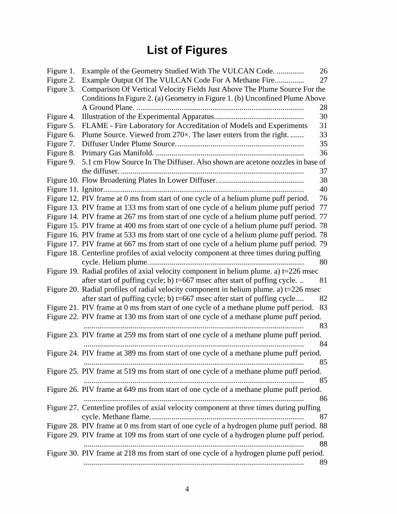
List of Figures
Figure 1. Example of the Geometry Studied With The VULCAN Code. .............. 26Figure 2. Example Output Of The VULCAN Code For A Methane Fire............... 27Figure 3. Comparison Of Vertical Velocity Fields Just Above The Plume Source For the
Conditions In Figure 2. (a) Geometry in Figure 1. (b) Unconfined Plume Above A Ground Plane. ...................................................................................... 28
Figure 4. Illustration of the Experimental Apparatus.............................................. 30Figure 5. FLAME - Fire Laboratory for Accreditation of Models and Experiments 31Figure 6. Plume Source. Viewed from 270×. The laser enters from the right. .......Figure 7. Diffuser Under Plume Source..................................................................Figure 8. Primary Gas Manifold. ............................................................................Figure 9. 5.1 cm Flow Source In The Diffuser. Also shown are acetone nozzles in ba
the diffuser. ..............................................................................................Figure 10. Flow Broadening Plates In Lower Diffuser. ............................................Figure 11. Ignitor.......................................................................................................Figure 12. PIV frame at 0 ms from start of one cycle of a helium plume puff period.Figure 13. PIV frame at 133 ms from start of one cycle of a helium plume puff periodFigure 14. PIV frame at 267 ms from start of one cycle of a helium plume puff periodFigure 15. PIV frame at 400 ms from start of one cycle of a helium plume puff periodFigure 16. PIV frame at 533 ms from start of one cycle of a helium plume puff periodFigure 17. PIV frame at 667 ms from start of one cycle of a helium plume puff periodFigure 18. Centerline profiles of axial velocity component at three times during puffi
cycle. Helium plume. ...............................................................................Figure 19. Radial profiles of axial velocity component in helium plume. a) t=226 mse
after start of puffing cycle; b) t=667 msec after start of puffing cycle. ..Figure 20. Radial profiles of radial velocity component in helium plume. a) t=226 ms
after start of puffing cycle; b) t=667 msec after start of puffing cycle. ...Figure 21. PIV frame at 0 ms from start of one cycle of a methane plume puff periodFigure 22. PIV frame at 130 ms from start of one cycle of a methane plume puff per
.................................................................................................................Figure 23. PIV frame at 259 ms from start of one cycle of a methane plume puff per
.................................................................................................................Figure 24. PIV frame at 389 ms from start of one cycle of a methane plume puff per
.................................................................................................................Figure 25. PIV frame at 519 ms from start of one cycle of a methane plume puff per
.................................................................................................................Figure 26. PIV frame at 649 ms from start of one cycle of a methane plume puff per
.................................................................................................................Figure 27. Centerline profiles of axial velocity component at three times during puffi
cycle. Methane flame. ..............................................................................Figure 28. PIV frame at 0 ms from start of one cycle of a hydrogen plume puff perioFigure 29. PIV frame at 109 ms from start of one cycle of a hydrogen plume puff pe
.................................................................................................................Figure 30. PIV frame at 218 ms from start of one cycle of a hydrogen plume puff pe
.................................................................................................................
4

List of Figures (Continued)
Figure 31. PIV frame at 328 ms from start of one cycle of a hydrogen plume puff period.................................................................................................................. 89
Figure 32. PIV frame at 437 ms from start of one cycle of a hydrogen plume puff period.................................................................................................................. 90
Figure 33. PIV frame at 546 ms from start of one cycle of a hydrogen plume puff period.................................................................................................................. 90
Figure 34. .Centerline profiles of axial velocity component at three times during puffing cycle. Hydrogen flame. ............................................................................ 91
Figure 35. Radial profiles of axial velocity component in hydrogen flame. a) 187 msec after start of puffing cycle; b) 546 msec after start of cycle at time of maximum necking ................................................................................................................. 92
Figure 36. Radial profiles of radial velocity component in hydrogen flame. a) 187 msec after start of puffing cycle; b) 546 msec after start of cycle at time of maximum necking. ............................................................................................................... 93
5
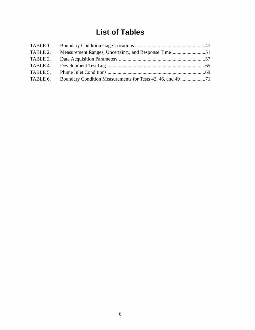
List of Tables
TABLE 1. Boundary Condition Gage Locations ........................................................47TABLE 2. Measurement Ranges, Uncertainty, and Response Time...........................51TABLE 3. Data Acquisition Parameters .....................................................................57TABLE 4. Development Test Log...............................................................................65TABLE 5. Plume Inlet Conditions ..............................................................................69TABLE 6. Boundary Condition Measurements for Tests 42, 46, and 49....................71
6

Nomenclature
Ra: Rayleigh number=
Re: Reynolds number = VD/ν
Ri: Richardson number =
g: Gravitational acceleration (9.81 m/s2)
dp: Seed particle diameter (µm)
D: Plume/burner inlet diameter (= 1 m)
P: Pressure (Pa)
T: Temperature (K)
V: Average inlet velocity given inlet flow rate (m/s)
α: Thermal diffusivity of the plume at the local T, P (m2/s)
µ: Absolute viscosity of plume fluid at local ambient T, P (Pa-s)
ν: Kinematic viscosity of plume fluid at local ambient T, P (m2/s)
ρair: Density of the air at local ambient T,P (kg/m3)
ρplume: Density of the plume at local ambient T,P (kg/m3)
ρp: Seed particle density (kg/m3)
τ: Characteristic seed particle response time (s)
ρair
ρplume---------------- 1–
gD3
να----------
ρair
ρplume---------------- 1–
gD
V2
-------
7

AcknowledgmentsAs with any large experimental effort, a number of individuals contributed to the design and conduct of the experiment. The authors would like to thank the following individuals:
• Rodney W. Oliver: Lead experimental technician
• Marty Martinez: Cinematography
• Thomas W. Grasser: PIV technician
• John J. O’Hare: Data acquisition technician
• Mark G. Mitchell: Laser system technician
• Benny Malone: Fabricator
• John Goldsmith/Scott Bisson: Laser system owners
The authors would also like to thank Walt Gill, Phillip Paul, Don McBride, Bob Cochran and Dan Aeschliman for technical advice on diagnostics and the design of the experiment.
This study was sponsored by the laboratory research and development program at Sandia National Laboratories which is operated by Lockheed Martin Corp. for the U. S. Department of Energy under Contract DE-AC04-94AL85000.
8
cal
nts.
image nce
ave ployed ancy
s duce
s of a er a d by
ent, er
ovie ly to the
scales g al was two
ld be
Executive SummaryThis report documents a Laboratory Directed Research and Development (LDRD) project to develop a diagnostic technique for simultaneous temporal and spatial resolution of fluid flows. The motivation for the research lies in the development and validation of numerical simulation capability for fluid flows. New numerical techniques, such as Large Eddy Simulation (LES), have temporal resolution capability that cannot be validated by traditional point measurements techniques such as laser Doppler velocimetry (LDV).
Four goals are defined for this LDRD:
• to demonstrate that velocity fields are measurable with two orders of magnituderesolution in two spatial dimensions and time, simultaneously
• to apply the PIV technology to study the physics of fully turbulent, buoyant, non-reacting and reacting flows
• to demonstrate that data sets of sufficient quality to support validation of numerisimulation tools can be obtained for buoyant, non-reacting and reacting flows
• to obtain simultaneous scalar field measurements with velocity field measureme
To achieve these goals, our approach has been to advance two techniques, particlevelocimetry (PIV) for velocity field measurements and planar laser induced fluoresce(PLIF) for scalar field measurements. While these non-invasive optical techniques hbeen under development in laboratory flows for several years, they have not been emat a scale sufficient to be of use for developing validation data in fully turbulent, buoydominated flows. To create these flows, the Fire Laboratory for the Accreditation of Models and Experiments (FLAME) was extensively modified to produce a canonicalplume flow from a 1 meter diameter source. Numerical simulation of the internal flowwithin the facility was used to guide the design of air inlets and plume placement to proa radial inflow as close to a unconfined round plume as is possible within the confinevented room. The confined geometry is necessary to obtain boundary conditions ovlarge fraction of the surface for use in validation of numerical simulations. As requireLDRD funds, significant leverage has been employed in using existing capital equipmincluding the FLAME facility, a very powerful (0.3 J/pulse) 308 nm, 200Hz, XeCl excimlaser borrowed from the Sandia Livermore Combustion Research Facility, 35 mm mcameras, and extensive high pressure gas hardware used to construct the gas suppplume.
Some 51 tests were conducted in the development of the PIV and PLIF diagnostics atuseful to turbulent plume flows. Tests were successfully conducted with non-reactinhelium, and reacting hydrogen and methane. Test results show that the first LDRD gomet. The developed PIV system in the FLAME facility demonstrated that quantitativevelocity field measurements were possible with two orders of magnitude resolution inspatial dimensions and time, simultaneously. For non-reacting plume flows, PIV cou
9

the
obtained across the full 0.8 m by 1.2 m field of view. For reacting-flows, the flow field velocities external to the reacting plume were measured and for methane flows, the non-reacting plume core was also measured. However, the hot product region was not measurable due to burn-up of the hollow glass seed particles chosen for this study.
The second LDRD goal was also met. Results have been obtained with the 1 meter diameter source for non-reacting helium, and reacting hydrogen and methane flows. The near source region of non-reacting and reacting plumes (fires) is an important flow for Sandia National Laboratories and has received little prior attention in the literature. It is the region in which baroclinic vorticity generation is the strongest while advected vorticity is the weakest. The data generated provide important insight into the dynamics of buoyant turbulence and its respective time and length scales.
The third LDRD goal can be met but was not in this study. Boundary condition measurement failures were the principal reason. However, with sufficient care, the identified problems can be eliminated. A measure of the confidence that these problems can be eliminated is that follow-on funding has been obtained from a defense program validation project to obtain validation data for a new fire numerical simulation tool currently under development.
The fourth LDRD goal may be obtainable but was met with partial success in this study. We were unable to obtain scalar field information in helium plumes because the acetone fluorescence signal was not strong enough. However, it is felt that through the use of an image intensifier, the weak images that were obtained could be amplified to the point of usability. While the fluorescence failed in the non-reacting helium fields, unexpected fluorescence signatures were gained in the reacting-flows. Of particular value is the signature in the reacting methane flows thought to be due to Polycyclic-Aromatic-Hydrocarbons (PAH’s). These signatures are a marker for the flame interfaces and information obtained is quite insightful.
10
IntroductionThis report documents a Laboratory Directed Research and Development (LDRD) project to develop a diagnostic technique for simultaneous temporal and spatial resolution of fluid flows. The original goals of the program were threefold. The first goal was to develop diagnostic techniques for obtaining two-dimensional velocity fields with two orders of magnitude resolution in both time and length scales. The second goal was to apply that technology to study the physics of buoyant non-reacting and reacting flows. The third goal was to demonstrate that data sets of sufficient quality to support validation of numerical simulation tools could be obtained by the technique. The program goals were expanded halfway through the first year of this two year project to include a fourth goal, that of simultaneous measurement of a scalar field with the velocity field.
The motivation for the research lies in the development and validation of numerical simulation tools for fluid flows. Simultaneous temporally and spatially resolved data sets are required to support a transition in computational fluid dynamics (CFD) simulation capability. For the past two to three decades, engineering CFD tools have employed a long-time average of the Navier-Stokes equations. The approach is called Reynolds Averaged Navier-Stokes (RANS). In RANS, it is commonly assumed that the discretization scheme is sufficient that the unresolved length scales smaller than the grid are homogeneous (and in many cases isotropic). This assumption of homogeneity allows for point measurements to be used for quantitative validation of the technique even if the discretization is large relative to the actual measurement volume.
Point measurements of velocity are typically obtained with Laser Doppler Anemometry/Velocimetry (LDA or LDV) probes or hot wire anemometry (HWA) in which a time-varying signal is obtained at a single point in space and then averaged with time. Typically, three orders of magnitude temporal resolution is obtained, but upwards of six orders of magnitude is sometimes acquired. Depending on the sophistication of the measurement devices, one, two, or three dimensional velocity signals can be obtained. To obtain spatial resolution, the measurement probe is moved from point to point in space and the temporal measurement repeated until the spatial resolution is obtained. For this single probe approach, there is no temporal correlation between the measurements at different spatial locations. Therefore, only time-averaged data has statistical meaning. Multiple probe measurements (probe arrays) are also sometimes used. If placed sufficiently close together, multiple probes can give an estimate of spatial coherence of the turbulence by cross-correlating the temporal signals of each probe.
Quantitative point measurement data are used to support numerical simulation in two ways. The data are used to validate the numerical simulation results and to develop turbulent closure models to account for the unresolved length scales. Because the RANS equations are time averaged, time-averaged data are sufficient for validation of RANS computations.
11
result terms , its
e
he S are d by
ocity is y, this
Large flows, l he
ce into cales. tial not
that lution. tion), s (such that
en point bulence
Therefore, velocity measurements obtained from an LDV probe, moved from point-to-point in space, is sufficient.
In RANS, turbulence is modeled as velocity fluctuations. In reality, turbulence manifests itself as both temporal and spatial velocity gradients. These gradients can be interpreted as “eddies” or “vortical structures”. These eddies overlap in length and time scales; the being chaotic (but not necessarily random). One means of characterizing an eddy is inof a characteristic length scale corresponding to its “coherence” and a characteristicvorticity corresponding to the velocity gradient. Regardless of the vorticity of an eddypassage through a point in space will manifest itself as a velocity fluctuation in time.
Because of time-averaging and homogeneity assumptions in RANS, the length scalcharacteristics of eddies are largely ignored. Hence, the RANS approach and point measurements are synergistic. Only through an autocorrelation can length scale information be extracted from point measurements (Tennekes and Lumley, 1972). Tprincipal characteristics of interest for the development of turbulence models for RANthe amplitude and frequency of the velocity fluctuations; both of which can be obtaineanalysis of point measurement data. The time-averaged root-mean-square of the velused as a measure of the turbulent kinetic energy. Plotted as a function of frequencamplitude decreases through the inertial range of turbulence.
Since the early 1960’s new numerical techniques that are not time-averaged, such asEddy Simulation (LES), have been under development (Smagorinsky, 1993). Thesetechniques have yet to reach the maturity to support engineering analysis in complexbut are expected to do so in the near future. LES shows great promise for numericasimulation technology. Its fundamental advantage over RANS is that it can resolve tlarge-scale, coherent, vortical structures commonly found in turbulent flow. In LES, volume averaging is employed which separates the length scale spectrum of turbulenresolvable (i.e., larger than the grid) and non-resolvable (i.e., smaller than the grid) sIn this manner, the turbulent motion captured on the grid has both temporal and spacoherence, i.e., it is composed of eddies. The turbulence with length scales that areresolvable are treated in the same manner as RANS, i.e., statistically.
In LES, the numerical simulation of turbulence with resolvable length scales impliesthe dynamics of eddies with spatial coherence are correctly represented in the grid soDynamic processes include growth mechanisms (such as baroclinic vorticity generadecay mechanisms (bursting and cascade to smaller scales), advection mechanismas stretching and pairing) and other dynamic vortical mechanisms. The assumptionLES solutions can in fact capture all of these phenomena for resolvable length scales cannot be validated by point measurements. No matter how many point measurements are takin a flow to provide spatial resolution, if there is no temporal coherence between themeasurements, the data cannot be used to validate dynamical phenomena. Since turhas both temporal and spatial gradients, temporal and spatial coherence in the measurements is required to show dynamical behavior.
12

Further, measurement technology such as quantitative photography, as Particle Image Velocimetry (PIV) is sometimes called, cannot be used to track dynamical phenomena with a velocity vector plot on a single time plane. The requirement to validate that a LES solution is correctly simulating dynamic, vortical processes is simultaneous temporal and spatial imaging with sufficient resolution in both time and space to resolve the dynamical phenomena of interest.
The temporal and spatial resolution required for validation depends both on the size of the computational model and the dynamical processes of interest in the flow that is to be modeled. At the current time, typical engineering flow computations on workstations solve less than a million nodes, which if evenly distributed in the three directions translates into less than two orders of magnitude node points per x, y, z direction. New massively parallel computers may permit up to a hundred million nodes, which translates into less than three orders of magnitude node points in each direction. We believe that two orders of magnitude in two spatial dimensions and time are achievable in this project, hence, that is the first goal of this LDRD.
The second goal of this LDRD is to apply that technology to study the physics of fully turbulent, buoyant, non-reacting and reacting flows. Many of the flows of interest to Sandia fall into this class. For example, safety applications (weapon and non-weapon) include mixing and combustion of fuel in a fire from solid, liquid, and gas sources (including shipping container foams, jet fuel, propane), and mixing of gaseous fuel with air (including military/civilian ullage vapors in fuel tanks). Environmental applications include smoke and particle (including radioactive) transport from fires and industrial applications. Energy applications include large industrial burners for waste incineration and energy generation.
All these flows involve scalar mixing in turbulent flows in which the entrainment is dominated by large coherent turbulent structures. All have integral length scales on the order of meters to tens of meters and integral time scales on the order of seconds to hours. Given the numerical simulation capabilities, minimum length scales resolvable on a grid can expected to be on the order of centimeters. Time scales for simulation depend on the tolerance of the user, since the simulation time depends on how long the computer runs. Typically, hundreds to thousands of time steps are simulated depending on the complexity and size of a problem. Therefore, temporal resolution can run from milliseconds to seconds depending on the problem.
A canonical flow was chosen in order to capture the salient features common to turbulent, buoyant types of flows. The canonical flow chosen is a simple round plume source with base diameter of one meter. Because of the interest in fires, it was chosen to study the turbulent plume motion from the base of the plume up to an elevation of about 1 diameter.
The third goal of this LDRD is to demonstrate that data sets of sufficient quality to support validation of numerical simulation tools can be obtained for buoyant, non-reacting and reacting flows. To achieve this goal, not only must simultaneous temporal and spatial imaging with sufficient resolution be obtained for the flow of interest, but the geometry, initial conditions and boundary conditions must also be specifiable with sufficient
13

resolution. Ideally, for specifying geometry, any objects with length scales on the order of the grid should be specified. For the most resolved computational grids for flows of order tens of meters, geometry above tens of centimeters should be specified. This level of resolution is reasonably achievable.
Ideally, initial condition measurements could be made at each node for each variable in the numerical solution, i.e., pressure, temperature, species, three components of velocity, etc. Since node counts will run from a million to a hundred million nodes, the number of measurements (all conducted at the same instant in time) runs from the tens of millions to billions. And of course, it would be nice if they were all non-intrusive. Obviously (to anyone who has ever conducted an experiment), this standard is not achievable with foreseeable technology. For the current series of experiments, the goal is to obtain data for quasi-steady flows. In quasi-steady flows, the effect of the initial transient dies away. Temporal variation is due to fluctuations which, if averaged over a sufficient number of cycles, do not change (i.e., ergodic). As a consequence, the measurement of initial conditions is relatively unimportant as long as the flow has sufficient time to reach a quasi-steady condition before measurements are taken.
Ideally, boundary condition measurements could be made at each surface node for each variable in the numerical solution at each instant in time that a time step is required by the numerical solution. For node counts in the million to hundred million range, surface nodes will run in the tens of thousands to millions. For time steps running in the thousands range with on the order of ten variables, the number of measurements required runs into the hundreds of millions to tens of billions. Obviously (to anyone who has ever conducted an experiment), this standard is not achievable with foreseeable technology. For the current series of experiments, the goal is to take a reasonable set of measurements with reasonable time resolution and to minimize the effect of the boundary conditions on the flow field of interest (by placing the flows in an enclosure, well away from inlets and outlet).
The fourth goal of the LDRD is to obtain simultaneous scalar field measurements with velocity field measurements. Unlike momentum driven flows in which scalars, such as species, tend to be uncoupled from the flow (i.e., passive), in buoyant flows, scalar fields do influence the momentum field (i.e., are coupled). In particular, the density of the species is important to the buoyancy. Therefore, it is of interest to have simultaneous measurements of the density field with the velocity field. Comparison of numerical simulation with this data will provide validation that the coupling is correctly represented in the simulation. The most direct means of measuring the density in a binary (plume/ambient) flow is to measure the concentration of either the plume fluid or the ambient fluid, assuming that their densities are known. In reacting flows, many species can be present. However, at a minimum, the flow can be defined as ternary, with fuel, oxidizer, and products. For buoyant flows, the reaction zones tend to be thin sheets (Tieszen, et al. 1996) while products diffuse into both the oxidizer and the fuel. Of particular interest is to identify either the flame zone or the edge of the products within the fuel or the air.
With a clear set of goals for the experiments, the number of technologies that can be applied to achieve those goals is limited. Gharib, 1996, has reviewed the technologies that may be
14

, hree-le
at we ws.
s now ded For a o-
tion of nly d on
y has ted cale,
used to support numerical simulation. He concludes that what is required to address the issue of turbulence is ‘quantitative visualization’. The ultimate goal is full, three dimensionaltemporal resolution. However, while advances are being made with holography and tdimensional particle tracking technologies, Gharib highlights the applicability of ParticImage Velocimetry (PIV) to measure two-dimensional velocity fields. For scalar filed measurements Planar Laser Induced Fluorescence (PLIF) is an option.
Measurement Technologies
For this LDRD project, PIV and PLIF have chosen as the measurement technologies thwould like to develop for measurements in fully turbulent reacting and non-reacting flo
In recent years particle image velocimetry (PIV) has been developed to the point that ibecoming a fairly standard measurement technique for two-dimensional velocity fields(Adrian, 1991). For PIV, a two-dimensional light sheet is created from a laser in a seeflow. Scattered light from the particles is recorded by a camera at two different times. well-seeded flow, such images directly provide flow field visualization. In addition, a twdimensional velocity field can be obtained by accurately measuring the spatial separathe particles between the two frames with well-known time separation. This techniqueprovides a spatially resolved velocity field, but not a temporally resolved velocity field. Owithin the last few years has PIV evolved to the point where images are being recordeCCD cameras to attain a measure of time resolution. However to date, PIV technologpredominantly been applied to low-speed, non-reacting, laboratory-scale flows of limirelevance to development and validation of numerical tools for fully-developed, large-sturbulent flows.
Many of the recent advances in PIV have been in the area of digital imaging, simplifying PIV by providing real-time feedback and eliminating the time-consuming task of film development. However, current digital camera and computer bus technology limits the acquired images to a certain number of pixels per second, limiting either the image resolution or capture rate. For this reason, the decision was made to use a hybrid PIV system, with high-speed film cameras for high spatial resolution imaging and sufficient frame rate to capture the dynamics of the flow, and high-resolution film digitization to allow fully digital processing. Willert (1996) discusses such PIV systems and their accuracy. The PIV system developed and applied here uses an excimer laser, 35-mm motion picture cameras, film digitization, and cross-correlation analysis.
PIV has recently been applied to helium plumes and small fires (e.g., Zhou and Gore, 1995) but not to large fires. The risk of such an endeavor is that, under certain circumstances, e.g., heavily sooting fires, PIV imaging may not be possible. In addition, volume expansion in reacting flows always makes proper seeding difficult. The large scale of the current setup provides an additional imaging challenge.
Planar Laser Induced Fluorescence (PLIF) is a recently developed laser-based diagnostic technique which has been successfully used for the measurement of gas species and
15

temperature in combustion environments. The principles of laser-induced fluorescence, upon which it is based, are well known. Briefly, a laser source is used to excite an electronic absorption transition in the species of interest. Following absorption, collisional redistribution of energy over the electronically excited state occurs. Following this redistribution, the molecule can return to the lower energy state through either collisional quenching or radiative de-excitation, the latter of which results in fluorescence emission. The fluorescence is typically collected at a right angle to the incident laser beam and measured using a photodetector, such as a photomultiplier tube for light detection at a single point, or an array detector such as a CCD (charge-coupled device) for multi-point imaging. One major difficulty with the application of this technique to chemically reacting flows is that the fluorescence yield is typically a function of the local gas composition and temperature. Thus spatial (and temporal) variations in these quantities can cause significant variations in the fluorescence yield. Since gas composition and temperature are typically not known a priori in turbulent flames, various schemes have been utilized to correct for variations in fluorescence yield and enable a quantitative relationship to be established between the measured fluorescence signal and the species concentration or temperature.
With the continued development of high powered lasers and more sensitive detectors, PLIF has been increasingly used to measure both major and minor species in laboratory scale flames. For example, PLIF has been used to measure the OH and NO concentration distributions in flames (Cattolica and Vosen, 1986; Kychakoff et al., 1984). More recently, the PLIF technique has been extended to other minor combustion species such as CH, C2 and CO (Allen et al., 1986; Haumann et al., 1986). In nonreacting flows, acetone, biacetyl, NO, NO2 have been seeded into the flow to act as tracers and provide data on turbulent mixing and flow structure (Lozano and Hanson, 1992). PLIF measurements of temperature have been demonstrated. For example, both OH and NO PLIF have been used to determine temperature by exciting the molecule at a single laser wavelength and detecting the resulting fluorescence signal at two different wavelengths corresponding to different molecular transitions (Seitzman et al., 1985).
The detection of intermediate hydrocarbon species by laser-induced broadband fluorescence has been reported by several previous investigators in diffusion flames (Smyth et al., 1985; Miller et al., 1982; Fujiwara et al., 1980). The resulting spectra from early studies obtained in the visible wavelength region have been attributed to Polycyclic Aromatic Hydrocarbons (PAH). More recent work in laminar diffusion flames extended these previous studies to detailed flame profiles of both visible- and ultraviolet-induced broadband fluorescence. In particular, Smyth et al. (1985) used an argon ion laser operating at 488 nm to excite broadband visible fluorescence, which was detected at 510 nm, and a frequency doubled Nd:YAG dye laser system at 282 nm to excite broadband fluorescence, which was detected at 345 nm. Detailed spectra show that the ultraviolet- induced broadband fluorescence extends from the excitation wavelength of 282 nm to about 425 nm with a maximum near 350 nm. Fujiwara et al. (1980) further showed that the broadband fluorescence can be obtained at excitation wavelengths between 260 and 310 nm and that the shape and position of the fluorescence peak is nearly independent of excitation wavelength. Other evidence suggests that the fluorescence originates from PAH’s of approximately 2 to 4 rings and that the excitation process involves a one-photon electronic
16

transition. The flame profiles show the peak PAH signal is confined to a relatively thin region on the fuel rich side of the high temperature reaction zone. While the width of the high PAH region is somewhat greater the high OH region (5 mm versus 2.5 mm for the OH) it is believed that the fluorescence signal attributed to PAH’s provides a useful indicator of the highly reactive flame zone.
PLIF is still primarily a laboratory scale diagnostic and has not been applied to larger scale flows. The primary risk in attempting to apply this technique to larger-scale, fully turbulent flows is that sufficient laser power may not be available to excite a measurable fluorescence signal. Further, in laboratory controlled environments it is fairly routine to add trace amounts of species known to fluoresce such as acetone, biacetyl, NO, or NO2. However, in larger-scale, non-reacting environments, these materials are either explosion hazards (acetone, biacetyl) or pollutants (NO, NO2).
Plumes/Fires
In keeping with the second goal of this LDRD, the flow fields of interest are fully turbulent, buoyant, non-reacting and reacting flows. These flows are also referred to as plumes and fires, respectively. For fires in particular, the programmatic interest is in the near source region, i.e., in the fire itself, not in the smoke plume high above the fire. It is both convenient and cost effective to have the same experimental setup apply to both non-reacting and reacting flow problems. Therefore, the focus of the current study will be on the flow characteristics in the region immediately above the plume source, i.e., within the first source diameter, for both reacting and non-reacting flows. A complete review of plumes and fire literature is beyond the scope of the current study. However, those characteristics of plumes and fires relevant to the current study, and velocity measurements made in them, are reviewed below.
Plumes
One would assume that plumes have received substantial attention in the literature. However, this assumption is not true. Compared to pure jet flows (momentum-driven), pure buoyant plumes have received very little study. Buoyancy effects on jets, called buoyant jets in the literature, have received substantial study. However, these mixed buoyant and momentum flows are not directly relevant to the current study in that the near source region of buoyant jets are momentum dominated, while they become buoyancy dominated only in the far-field. Because of our focus on the near source region, buoyant jets are still likely to be momentum dominated in this region.
The issue of momentum vs. buoyancy is not just related to mean field characteristics but carries over into turbulence. Tieszen, et al. 1996, argue that baroclinic vorticity generation is an important mechanism in plumes and fires. Baroclinic vorticity generation occurs when density and pressure gradients are misaligned and results in the production of rotational motion. At the plume/air interface a strong, mostly horizontal density gradient exists. At the same location, even in the absence of motion, there is a mostly vertical pressure gradient
17
f l, most plume n on d vected
en and uffing , since d ffing
n for
he vate
due to hydrostatic loads. As a result, there is a generation term that exists at the edge of the plume. Away from the plume/air mixing layer, there may not be any density gradients interior to the plume or in the ambient air, so there may be no source of vorticity production there.
However, the ratio of the vorticity generated locally to the vorticity advected into the plume/air mixing layer decreases as the distance increases from the source. There are two reasons. First, the vorticity generated upstream of a given point will be advected along with the flow, and therefore, some fraction of the vorticity produced in the plume/air interface will end up downstream along the interface as well. Second, as mixing occurs, and the mixing layer thickens, the density gradient between the plume and air broadens and the baroclinic vorticity production rate slows. The combination of decreased production and increased advection contributes to a decreased importance of the local buoyant production of turbulence. For example, in the self-similar region (far from the source) of a hot air jet, Shabbir and George, 1994, conclude “It is found that even though the direct effect obuoyancy in turbulence, as evidenced by the buoyancy production term, is substantiaof the turbulence is produced by shear....Therefore, it is concluded that in a buoyant the primary effect of buoyancy on turbulence is indirect, and enters through the meavelocity field (giving larger shear production).” We expect that the effect of buoyancyturbulence in the near source region to be more direct than that found by Shabbir anGeorge since the production is strong (due to sharper gradients) and the amount of advorticity is relatively lower.
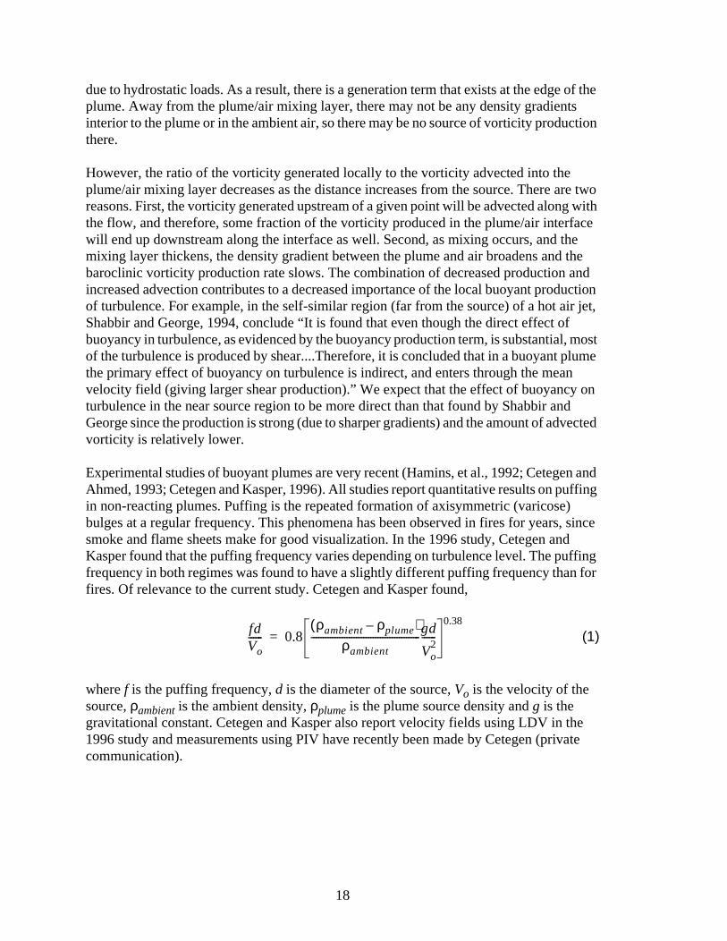
Experimental studies of buoyant plumes are very recent (Hamins, et al., 1992; CetegAhmed, 1993; Cetegen and Kasper, 1996). All studies report quantitative results on pin non-reacting plumes. Puffing is the repeated formation of axisymmetric (varicose)bulges at a regular frequency. This phenomena has been observed in fires for yearssmoke and flame sheets make for good visualization. In the 1996 study, Cetegen anKasper found that the puffing frequency varies depending on turbulence level. The pufrequency in both regimes was found to have a slightly different puffing frequency thafires. Of relevance to the current study. Cetegen and Kasper found,
(1)
where f is the puffing frequency, d is the diameter of the source, Vo is the velocity of the source, ρambient is the ambient density, ρplume is the plume source density and g is the gravitational constant. Cetegen and Kasper also report velocity fields using LDV in t1996 study and measurements using PIV have recently been made by Cetegen (pricommunication).
fdVo------ 0.8
ρambient ρplume–( )ρambient
----------------------------------------------gd
Vo2
------0.38
=
18

Fires
Fires are a topic of general interest to Sandia for safety reasons. For the purpose of this study our interest is limited to external fires, i.e., a simple round reacting plume. The most common problem for which this geometry is applicable is a pool fire, i.e., a fire above a liquid hydrocarbon pool. Our intent experimentally is to decouple the vaporization of the liquid by using gaseous fuels to simplify the experiment. However we want to have the same vapor flow rate as that occurring in a pool fire.
Blinov and Khudyakov, 1961 show that vaporization rates are a function of the diameter of a fire. However, for fires above about a meter in diameter, the mass loss rate is fairly constant at about 5 mm fuel per minute (about 0.065 kg/m2/sec). Blinov and Khudyakov also classify fires as being laminar if the base diameter is below about 10 cm in diameter and transitional between 10 cm and 1 meter. Above 1 meter the fires are considered fully turbulent. The meaning of transitionally turbulent vs. fully turbulent is not completely clear.
We speculate that the meaning of fully turbulent is that the flow is sufficiently turbulent that the flame zone is optically thick over much of the pool surface. What we mean by optically thick is that it is rolled and folded so that multiple sheets exist between the liquid surface and the cold environment. Smaller fires have spoke like structures but do not appear to be multiply folded until reaching the central plume (see for example, images from Weckman and Sobiesiak, 1988; Cetegen and Ahmed, 1993). Blinov and Khudyakov show that the mass loss rate of fuel increases with increasing diameter from a minimum for fires with diameters around 10 cm until the diameter reaches about 1 meter. This increase is consistent with an explanation that the flame zone is increasing its optical thickness as the diameter gets larger because the turbulence gets stronger.
Like plumes, fires are characterized by strong puffing (Malalasekera, et al., 1996; Cetegen and Ahmed, 1993; Hamins, et al., 1992). Cetegen and Ahmed plot data from a number of sources ranging over three orders of magnitude in length scale and give a curve fit of the puffing frequency as
(2)
where f is the puffing frequency and d is the diameter of the source.
PIV and PLIF have been applied to laboratory scale jet flames by a number of researchers and very recent work by Zhou and Gore (submitted for publication) has used PIV on small fires. The most advanced velocity measurement technique that has been applied to turbulent fires has been LDV (Weckman and Strong, 1996; Crauford, et al., 1985; Zhou and Gore, 1995). The LDV application of Weckman and Strong is the largest fire to which LDV has been applied. Their fire has a 0.31 m base diameter, still classified as transitionally turbulent by Blinov and Khudyakov definition. Their test data includes very detailed turbulence characteristics including buoyant production of turbulence. In comparison,
f1.5
d-------=
19

sented
ic
ments lear
Zhou and Gore’s data is for a 0.07 m base diameter fire, and measurements are preonly for the air inflow. However, Zhou and Gore manipulate their data to show that azimuthal vorticity occurs at the flame/air interface in support of the hypothesis that baroclinic vorticity generation is the dominant contributor to the vorticity in the flow.
For fires larger than 0.31 m in diameter, flow velocity has been inferred from dynampressure measurements made with thermally hardened pitot tubes (McCaffrey and Heskestad, 1976, Kent and Schneider, 1987). The most extensive velocity measuretaken in a fire with hardened pitot tubes at Sandia NationaL Laboratory is in the NucWinter Tests (Schneider, et al., 1989).
20

t that scale ong ted is tain nt
s fully
rest
o he scale nsity
sity of f
na is y. The
Description of ApparatusThere were a number of design constraints that were considered in the experimental apparatus. These issues will be reviewed in the next section followed by a detailed presentation of the experimental hardware and diagnostics.
Experimental Design Issues
In order to meet the goals of the LDRD program, design compromises had to be made. To build and implement measurement techniques, it is desirable to have the scale of the experiment be as small as possible. Minimum scale permits the fastest turn-around-time for experiments, the highest data density for a fixed number of boundary condition measurements, and the lowest laser power requirements for PIV and PLIF. In short, minimum scale meets the ‘new’ NASA paradigm which is sweeping the scientific community: better, faster, cheaper.
On the other hand, the buoyant flows need a minimum scale to become fully turbulenis typically much larger than momentum driven flows which can be studied in a small laboratory environment. Unlike momentum driven flows in which vorticity is created alinterfaces with solid objects in the flow, turbulence in buoyant flows is primarily creawithin the domain due to baroclinic vorticity generation. For most momentum drivenapplications in which the Reynolds number is reasonably high, the transition region limited to a small fraction of the flow, e.g. leading edge of a wing. It is desirable to obthe same flow conditions in the buoyant flow experiments, i.e., the laminar-to-turbuletransition occur at a small elevation above the plume source so that most of the flow iturbulent. In this way statistics from the flow can be used for validation of numerical simulation tools designed for fully turbulent flows (which occur in applications of inteto this LDRD).
Reacting flows are anticipated to remain more laminar than non-reacting flows for twreasons. First, reacting flows involve dilatation of the flow field which is manifest in theat release region of the flame zone. Dilatation results in a sink term in the vorticitytransport equations (Tieszen, et al., 1996) which will tend to slow the rotation of small eddies locally within the primary heat release zone in a flame. Second, due to the dechanges associated with high temperatures within the products, the kinematic viscothe products is much higher than the ambient temperature reactants. The diffusion ovorticity is directly proportional to the kinematic viscosity, which results in a loss of vorticity in these higher temperature regions. Another way of describing the phenometo say that the local Reynolds number drops due to the increased kinematic viscositdecrease in Reynolds number tends to ‘laminarize’ the flow.
21

Hence, we conclude that reacting flows will have longer laminar-to-turbulent transition distances compared to non-reacting flows. For this reason, we chose reacting flows to set the scale of the experiment for an acceptable laminar-to-turbulent transition distance relative to the scale of the experiment.
Unlike momentum driven flows, in which the transition distance can be arbitrarily shortened by increasing the inlet flow velocity (Reynolds number) for a fixed scale, in buoyant flows one cannot arbitrarily increase the baroclinic vorticity generation rate in the bulk flow. To increase the baroclinic vorticity generation rate requires that either the pressure gradient be increased or the density gradient be increased. It is difficult to increase the pressure gradient (here on earth) without introducing significant amounts of vorticity advected from walls which would not be present in a real flow. The density gradient can be increase arbitrarily up to a limit through the choice of plume and ambient fluids. In gases, the lightest ambient fluid is hydrogen (2 g/mol), the heaviest that is commonly available is perhaps sulfur hexafluoride (146 g/mol). In commonly available liquids, the lightest is perhaps a light hydrocarbon fuel (S.G. ~ 0.5) and mercury (S.G. = 13.6).
However, having chosen to study reacting flows as well as non-reacting flows due to the interest in fires, the choices of plume and ambient fluids are substantially limited. The plume fluid must be a fuel and the ambient fluid must be an oxidizer. Reacting jets in liquids have been previously studied (c.f., Dahm and Dimotakis, 1987; Mungal and Frieler, 1988) but the chemistry was chosen so that the heat release was limited. Further, liquids typically have very different diffusional length scales between momentum and species (Sc on order of hundreds) while in gases, the diffusional length scales are more nearly equal (Sc on order of unity). To avoid these complications, we choose to study gaseous flows.
For gases, it is most convenient to allow the ambient oxidizer to be air. It is cheap, readily available, convenient to use, and poses no health risks. Therefore, maximizing the baroclinic vorticity generation equates to minimizing the density of the plume fluid. For reacting flows, hydrogen is the lightest element, while for non-reacting flows, helium is the lightest element. Hence, both hydrogen and helium are chosen as plume fluids for these experiments. However, hydrogen chemistry is significantly different than hydrocarbon chemistry and hydrocarbon fires are a reacting flow of direct interest. Therefore, the lightest hydrocarbon, methane, is also chosen as a plume fluid for these experiments. Since methane has the least density difference with air, it is expected to have the largest laminar-to-turbulent transition distance of any of the three plume gases chosen.
After maximizing the baroclinic vorticity generation in the experiments, the only other means of reducing the fraction of the flow undergoing a laminar-to-turbulent transition is to increase the scale of the experiment. Of course this directly conflicts with the need to minimize the scale of the experiment for diagnostic purposes. As a result, a balance is needed. Since flows with a hydrocarbon fuel will have the longest laminar-to-turbulent transition distance, we chose fires to pick the optimal balance between the competing needs for scale. We rely on the classical pool fire categorization of Blinov and Khudyakov, 1961, who describe fires as being laminar up to base diameters of about 0.1 meter, transitionally turbulent for base diameters from about 0.1 meter to 1.0 meter, and fully turbulent above
22
1.0 meter. Based on this description, we choose a plume with a base diameter of 1.0 meter as a balance between the need to minimize the laminar-to-turbulent transition length in the flow and the need to minimize the flowfield for diagnostic purposes.
Having chosen the scale of the base of the plume, it is necessary to determine the overall scale of the experiment. The highest power/fastest pulse rate combination that we could obtain in a laser system for these experiments is 0.3 J/pulse, 200 pulses/sec. Given the laser power, it was decided that a sheet height for PIV measurements of 0.5 meters was achievable and 1.0 meter was potentially possible. Further, it was possible that this sheet could penetrate a 1.0 meter diameter flow and the scattered light still be sufficient to be detectable. Of concern were reacting flows with methane which are sooting. If the soot density is sufficiently high the optical path length could shorten to less than a meter. Therefore, a 1 meter by 1 meter image was deemed the optimal starting point for imaging with some risk that reacting methane flows with a base diameter of 1 meter may not be imageable.
The one meter by one meter image box could have reasonably been placed anywhere desirable within the flowfield. It was chosen to place this measurement box just above the plume source and bisecting it for three reasons. First, the inlet to the measurement box also is the boundary condition of interest on the exit plane of the plume. So the measurements serve dual purpose as a test plane within the flow and as boundary condition measurements on an important boundary. Second, the near source region of plumes has received far less attention in the literature than the far-field where the flow becomes self-similar. The near source region is where the least mixing has occurred between plume and ambient fluids, hence the baroclinic vorticity generation is maximized while the level of advected vorticity is minimized in this region. Third, for fully turbulent fires, the Blinov and Khudyakov data show that the flame height is only two to three times the base diameter. Therefore, a significant amount of the fuel is consumed within the first diameter. Further, for large fires (base diameters of 5 meters or greater) of interest for safety purposes, the flow above the fuel spill is of primary interest for heat transfer to weapons systems (crash and burn problem).
For scientific archival purposes, it is desirable to conduct an experiment which is as clean as possible and relevant to the physics of interest. The cleanest possible experiment for a plume is a free standing plume in an infinite atmosphere with no geometry other than the plume source. For the fire problem, a ground plane must be added. The cleanest possible geometry in this scenario is to have the plume source coincident with, and perpendicular to, the ground plane. In either problem, the simplest flowfield is an infinite, (or, more precisely, semi-infinite for the case with a ground plane) stagnant flowfield other than the flow induced by the plume. One-dimensional cross-flow is also of interest, particularly for the fire problem. However, for the purposes of this LDRD, it was decided to focus on the simpler plume in a ground plane with otherwise stagnant ambient fluid.
Unfortunately, the need for a semi-infinite flowfield to have a canonical flow for research purposes conflicts with the need to minimize the scale of the experiment in order to properly measure boundary conditions. Boundary conditions specified at infinity are a
23

great theoretical exercise but impractical for placing measurement probes. It is desirable to minimize the surface area of the experiment in order to maximize the measurement density for a fixed number (cost) of measurement devices. If probes are placed too close to the plume for boundary conditions, then the radial inflow from the plume will affect the measurements, i.e., they will not be stagnant, but dependent on the flow. Placing the boundary measurements at large distances from the plume implies a great number of measurements for a given measurement density.
Moreover, an even more significant problem exists in the control of ambient fluid to create a stagnant atmosphere into which a meter size plume can be flowed. Plumes are very sensitive to small shifts in momentum due to the fact that they have little momentum themselves. Simply placing a plume in an outdoor environment on a flat surface is likely to be successful only under a very limited set of weather conditions. It not only requires absolutely dead calm but uniform solar illumination just sufficient to bring the ground temperature in equilibrium with the air temperature to suppress natural convective plumes on the surrounding plane.
The combination of inability to control stagnant conditions in the plume plus the large number of measurements to specify boundary conditions far from the plume suggests that the plume needs to be brought into an enclosed environment so that boundary conditions can be controlled to a greater extent and can be specified to a reasonable density. For boundary condition measurements as well as computational mesh size requirements to compare with the experiments, it is desirable to minimize the enclosure volume.
In soliciting input from experimentalists and analysts in the fire area at Sandia National Laboratories, it was a consensus opinion that boundaries should not be placed closer than about three diameters from the fire if the effects of the boundary on the fire are to be minimized. This opinion is based on experience with numerical simulations in which the fire simulation is effected by the boundary conditions, if it is much closer than three diameters from the source. Obviously, this experience is somewhat qualitative, but indicates that a facility with walls 6 to 8 meters apart is needed to minimize wall effects for a 1 meter diameter plume. Fortunately, an existing facility, the Fire Laboratory for Accreditation of Models and Experiments (FLAME) (to be described below), fits these general guidelines, having a central chamber 6 meters in each coordinate direction. Therefore, FLAME was used as the experimental enclosure.
Because momentum boundary conditions are easy to specify on solid walls, e. g., no-slip, the use of the enclosure reduced the area required for momentum boundary condition measurements to inflow and outflow areas. Smaller inflow and outflow areas increase the measurement density for a fixed number (cost) of measurement devices. However, smaller inflow/outflow areas mean higher inlet/outlet velocities and correspondingly, higher momentum entering/exiting the enclosure. Further, enclosures are notorious for producing complex flow patterns. Since plumes are strongly affected by high momentum flows, it is necessary to diffuse the momentum associated with inlet/exit conditions within the enclosure and to position the plume as far from inlet/exits as possible.
24

Because of the desire to have a simple radial inflow for scientific purposes in spite of the inherent complexities of enclosure flows, and the need to balance inflow/outflow area vs. measurement density, the flow patterns within the enclosure were modeled with a computational fluid dynamics (CFD) code. The CFD code used was VULCAN, a joint development of Sandia National Laboratories and SINTEF/NTNU, and is based on the KAMELEON II Fire code developed at SINTEF/NTNU, Norway (Holen, et al., 1990). The code calculates RANS solutions for non-reacting and reacting flows using a finite volume representation of the basic equations of fluid dynamics, using mathematical submodels to represent the remaining physical phenomena. Key submodels include the k-ε turbulence model (Launder and Spaulding, 1974), a turbulent Schmidt number for scalar transport, and for reacting flows, the Eddy Dissipation Concept combustion model (Magnussen, et al., 1979), and a soot model (Magnussen, 1981). For reacting flows, thermal radiation is solved using a three-dimensional, discrete transfer model (Shah, 1979). The calculations are three dimensional and elliptic, and use a false transient to reach steady-state.
An example of the geometry studied is shown in Figure 1. Approximately 100 simulations were conducted to position the plume source above the air inlets, set the ground plane dimensions around the plume source, the geometry and area of the air inlets, and internal geometries to control the flow. Various inflow conditions were specified including free draw (constant pressure) and forced flow (constant velocity). For the plume, turbulence properties were assigned based on assuming the RMS fluctuating velocity is equal to the inlet velocity and length scale of the fluctuations is equal to 2.5 mm (on the expectation that the plume source would be through a ceramic porous plate to take the heat load of the reacting flows). For the air inlets, turbulence properties were assigned based on assuming that the RMS fluctuating velocity is equal to 10% of the inlet velocity and the length scale of the fluctuations is equal to 6.25 mm (on the expectation that the air source would be through 1/4 inch cell honeycomb). Standard temperature and pressure were assumed, as was the composition of the plume (helium - nonreacting and methane - reacting) and the surroundings - air. To reduce the grid size, quadrant symmetry was assumed.
Sample output from the calculations for a methane fire is shown in Figure 2. The basic design premise is that a vertical annular coflow will not remain a coflow within the enclosure with a sufficiently wide lip (ground plane) on the plume. Rather, the buoyancy of the plume will result in the coflow being drawn radially inward over the lip (ground plane) of the plume and into the base of the fire. In addition, near the top of the facility, where the ceiling tapers into the chimney, the remaining annular coflow is forced radially inward to escape the narrower chimney. As a result, a fairly uniform radial entrained air inflow results from what looks like a nominally annular coflow geometry. Note that by assuming quadrant symmetry in the calculations, real flow modes without x-y symmetry that may exist in the facility are not captured in the calculations. In other words, radial symmetry was assumed in the calculations, it was not proven to exist by them. However, subsequent experience with the facility indicated that indeed the flow was basically symmetric for the desired test conditions. (Not a given outcome, since enclosures are notorious for producing complex flow patterns).
25

A comparison was made for the final geometry chosen with a simple unconfined plume, both non-reacting and reacting. Figure 3 shows a comparison of the vertical velocity along a two-dimensional vertical plane passing through the center of the plume just above the plume source for the geometry in Figure 1 using the flow conditions in Figure 2 and similar conditions in an unconfined plume. The comparison is quite good. Since the tool was used as a screening tool, the comparison in Figure 3 has to be taken as qualitative. However, by placing the plume source at an elevation between 1/3 and 1/2 of the facility height, the region of the plume of interest for measurements occurs in the center of the facility, thereby, maximizing the distance available for diffusing the inlet/exit momentum. Further, by using fairly large inlet ducts to minimize the inlet flow velocity, the code predictions indicated that the plume will behave similar to an unconfined plume. This level of
Figure 1. Example of the Geometry Studied With The VULCAN Code.
26

assurance is the best that can be achieved given the desire for a radial inflow in a small enclosure.
Having established the scale and location of the plume, trade-offs were also required for the composition and momentum range of the plumes that could be studied. For generality, one would like to vary the composition of the plume fluid to change the plume density, and thereby, the baroclinic vorticity generation rate. As an example, by varying mixtures of helium with nitrogen (which has very nearly the density of air) the effects of the density gradient between the plume and the air can be studied. The creation of binary mixtures of
Figure 2. Example Output Of The VULCAN Code For A Methane Fire.
27
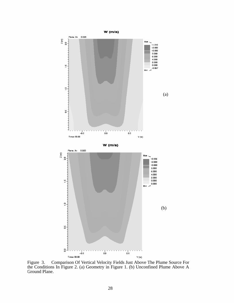
Figure 3. Comparison Of Vertical Velocity Fields Just Above The Plume Source Forthe Conditions In Figure 2. (a) Geometry in Figure 1. (b) Unconfined Plume Above AGround Plane.
(a)
(a)
(b)
28
plume fluid complicates the experiment and doubles the cost of the gas supply system. However, the capability was deemed worth the cost and the ability to create binary mixtures of plume fluid was implemented.
Also for generality, one would like to study the full range of buoyancy to momentum ratios (Richardson number) from plumes to jets. However, having chosen a 1 meter diameter source, both gas flow and measurement frequency requirements restrict the upper end of the velocity range and flow duration that can reasonably be achieved. Through a cost/benefit trade-off, taking into account existing hardware that could be applied to this study, it was determined that an upper bound source velocity of about 0.5 m/s with a duration of about 60 seconds was achievable at acceptable cost. This level is sufficient to study reacting plume sources with the same heat release rate as liquid hydrocarbon pool fires of the same base diameter.
Given a source velocity on the order of tenths of meters per second, and acceleration due to buoyancy, maximum flow velocities on the order of meters per second are expected. This level is consistent with achieving two orders of magnitude in resolution in time and space, for PIV measurements in a 0.8 m by 1.2 m view with 200 frames/sec. Achieving two orders of magnitude in space, requires PIV interrogation areas on the order of a centimeter on a side. With maximum velocities on the order of meters per second with 200 frames/sec, the particles will travel on the order of centimeters or less. Hence, particles will remain within the interrogation area, which is optimal for PIV measurements. Source velocities higher than meter per second levels would not be measurable with equipment available within this LDRD.
Experimental Apparatus
Based on the compromises required to balance the competing experimental goals and the results of the numerical design simulations, the basic design illustrated in Figure 4 was chosen for fabrication. Details of the hardware are presented in this section. To designate locations, two coordinate systems have been established. Obviously, a single coordinate frame of reference is preferable, however, the geometry is not conducive to a single system because the FLAME facility itself is square, while the experiment is designed to be axisymmetric. Therefore, one coordinate system is used for the FLAME building and a second coordinate system for the experiment itself.
Both coordinate systems have their origin (0,0,0) at the center of the surface of the plume source. To avoid confusion as to which system is intended, coordinates for the FLAME facility will be called out as North, South, East or West with an elevation relative to the plume source. The south wall is the wall facing the viewer in Figure 4. As a reference, the facility doors are on the south wall. For all other hardware and instrument locations, a (r,θ,z) coordinate system is established. The zero degree angle corresponds to the incident beam direction in Figure 4 with counter-clockwise being positive. For purpose of discussion, the description of the experimental apparatus will be divided into three parts, the building, the plume hardware, and the air duct hardware.
29

FLAME BuildingFigure 5 shows the Fire Laboratory for Accreditation of Models and Experiments (FLAME). Overall, the facility contains a central chamber containing the experimental apparatus, a long chimney centered over the central chamber, and external hardware to supply air to the central chamber and cooling water to the walls. Modifications made to the
Figure 4. Illustration of the Experimental Apparatus.
30

facility for this LDRD include extensive internal structures for air and plume gas sources, and external high pressure gas delivery system for the plume source.
The central chamber is a nominally 6.1 m (20 ft) cube. The floor of the facility is 2.45 m below the plume source. The floor is flat with a subfloor in the center of the chamber 0.51 m below the main floor. The subfloor is 3.05 m on a side and is centered under the chimney. The bottom and four sides for the FLAME facility are enclosed except for four air inlets into the lower four corners of the facility. The ceiling is not horizontal but tapers upward toward the opening to the chimney at the center of the facility. The ceiling taper is 32 degrees (from the horizontal) beginning at 3.55 m above the plume source and ends at the opening to the chimney. The chimney opening is at an elevation of 4.56 m above the plume source. The chimney is square in cross-section, nominally 2.3 m (7.5 ft) on each side, and extends an additional 7.32 m (24 ft) above the central chamber.
The facility is made principally of 0.305 m wide by 0.102 deep (12 in by 4 in) channel with a nominal 4.75 mm (3/16 in) wall thickness. The channels are interconnected to allow a cooling fluid (glycol/water mix) to be pumped through the walls to cool them. Because of the short duration of the fires in this program, this cooling was not required. The ceiling and a 1.2 m high segment of the side walls where it joins the ceiling are protected with a 1.6 mm thick stainless steel radiation shield. These shields are mounted with a 10 cm offset into the facility to provide thermal protection for large, long duration fires. An outer structure
Figure 5. FLAME - Fire Laboratory for Accreditation of Models and Experiments
31

of steel beams is used to provide additional structural reinforcement to permit a small internal explosion without damage to the facility. Access to the facility is through two large doors, 1.52 m (5 ft) wide by 5.49 m (18 ft) high located in the center of the south wall.
During normal operation the access doors are closed and the only inlets to the facility are from the plume and ambient air sources, and with one small exception, the only exhaust is through the chimney. The hardware associated with each of these sources will be discussed separately in the following sections. The one small exception is a small hole that exists within the central chamber through which gases can be exchanged with the outside world. This hole is 0.05 m in diameter and is located at (r,θ,z) = (4.31 m, 0°, 0.0 m). The purpose of the hole is to allow the laser through to the facility. The hole could be closed by a quartz window but each window results in a loss of laser power. Also the doors on the south face of the facility are intended to be closed tightly, however, due to their size, some small leakage can be expected. Relative to the source areas and exhaust area, these leaks are negligible.
32

Plume SourceThe plume source for these experiments is shown in Figure 6. The diameter of the source is 1.00 meters and is surrounded by a 0.51 m wide sheet steel lip which represents the ground plane. The centerline of plume is coaxially located with the center of the central chamber and the chimney to within approximately 5 cm. The center of the plume at its surface is the location of the coordinate system origin, (r,θ,z) = (0, 0°, 0).
The material at the surface of the plume source is a 2.54 cm thick porous ceramic plate with nominal pore size of 2.5 mm (10 pores per inch). The ceramic was manufactured in 90° wedges and cemented together with ceramic cement. The cement lines are nominally the thickness of the pore webbing so as to not create excessive flow blockage. However, they have been rotated out of the plane of the laser sheet to minimize distortion to the measurements.
The surface of the ground plane surrounding the plume source is made of 4 mm plate steel and is uniform to within about 6 mm. The ground plane is supported on a 2.9 cm thick steel grating backup held on unistrut supports which carry the weight into a welded steel frame
Figure 6. Plume Source. Viewed from 270°. The laser enters from the right.
33
from
oduce ter per
ssure s are tem a test. n the ssure safety ured. f flows. hese of the
used for support. With the exception of one square cutout, the surface of the ground plane is continuous with aluminized tape to seal joints within the lip, and between the lip and the plume. The square cutout is located at the edge of the plume source at an angle of 270°. The hole is 0.05 m circumferentially by 0.09 m radially and permits access to the plume for an ignitor system mounted under the ground plane.
The plume source rests upon a large diffuser which is part of the gas flow system for the plume. The diffuser, shown in Figure 7, is approximately 3 meters tall and extends down 0.51 m below the main floor of the facility to a subfloor at the center of the chamber. The diffuser is nominally 1.0 m in diameter for 1 m below the plume source. A pressure relief vent in the waist of the diffuser increases its diameter to 1.2 m for 0.27 m. Below the relief valve, the diffuser has a diameter of 0.95 m to the floor level. Below floor level it has a hemispherical lower head. The material in the upper part of the diffuser is 3 mm thick steel sheet stock while in the lower part it is 18 mm thick stainless steel.
Functionally, the plume source consists of up to four fluid streams, mixed upstream appropriately. Two streams are used to control the gaseous composition of the jet to allow binary mixtures within the plume to be studied. In addition, vaporized acetone was injected for PLIF studies and particles (to be described in the diagnostics section) were injected for PIV studies. To produce the plume flow, five independent gas systems were required. The five systems are the primary plume gas flow, the acetone liquid flow, the particle flow, the ignitor gas flow, and pneumatic valve control flow. Each will be described below.
Primary Plume Gas Flow: Prior to this LDRD the FLAME facility did not have any means of supplying gaseous fuels. The gas supply system was designed and fabricated for these tests. A large portion of the components of the system came from previous gaseous combustion studies under an earlier LDRD (Tieszen, Stamps, and O’Hern, 1996).
The gas composition of the plume is created from two independent gas lines leadingcompressed gas bottle farms. Each line is supplied by six 43.8 liter compressed gascylinders each containing nominally 7.7 m3 of gas at local ambient conditions. The two high pressure flows are regulated to intermediate pressure, measured, choked to prindependence, mixed, and then diffused to produce a low velocity (less than one mesecond) flow across a one meter source.
Figure 8 shows the complexity of the manifolds required to create the flows. High pregases flow into the manifold from the bottle farms at a maximum of 14 MPa. The linevalved so that the “diluent” side can flow into the “fuel” side to allow purging of the syswhen combustible gases are used, although the two lines flow independently during The flows are passed through filters to remove dust from gas bottle storage and thepressure is dropped to nominally 1.4 MPa by high-flow-rate (Circle Seal SR800) preregulators. As with all gas systems, manual and pressure relief valves are present forpurposes. The pressure, temperature and flow rate of the gas in each line are measHigh and low range flowmeters are used to ensure accuracy across a broad range oThe flow in each line then passes through a flow controller valve (Jordan Mk 708). Tvalves are run under choked conditions such that the upstream flow is independent
34
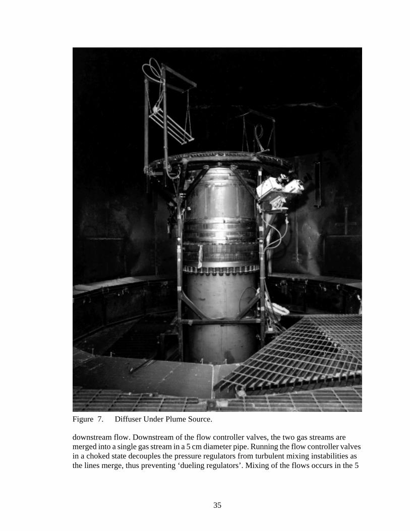
e 5
downstream flow. Downstream of the flow controller valves, the two gas streams are merged into a single gas stream in a 5 cm diameter pipe. Running the flow controller valves in a choked state decouples the pressure regulators from turbulent mixing instabilities as the lines merge, thus preventing ‘dueling regulators’. Mixing of the flows occurs in th
Figure 7. Diffuser Under Plume Source.
35

the tes by the son),
cm diameter pipe which runs through nominally 4.5 m and three 90° elbows before being dumped into the diffuser.
The final element within the primary gas flow system is the diffuser. The flow exiting the top of the diffuser is the plume source. The gas enters the base of the diffuser through the 5 cm tube in the center of, and aligned coaxially with, the diffuser as shown in Figure 9. Depending on the flow rates, the pressure in 5 cm tube may be sufficiently high to choke at its exit into the 0.91 m internal diameter of the lower part of the diffuser. In any case, the diffuser area is so large that the pressure in the diffuser is nearly ambient. The resulting jet flow into the lower portion diffuser is broadened out by a series of four plates with decreasing hole diameters (2.5 cm, 1.9 cm, 1.3 cm, and 0.95 cm) but relatively fixed blockage ratio of approximately 0.5, as shown in Figure 10. The plates and spacing between them is taken from a proven diffuser design used in Sandia’s wind tunnels. Each of plates is backed up by grating to provide support for the drag loads placed on the plathe diverging jet. The final plate is backed up by 10 cm thick grating. It is bolted intodiffuser with spring loaded bolts such that if the plate becomes plugged (for any rea
Figure 8. Primary Gas Manifold.
36
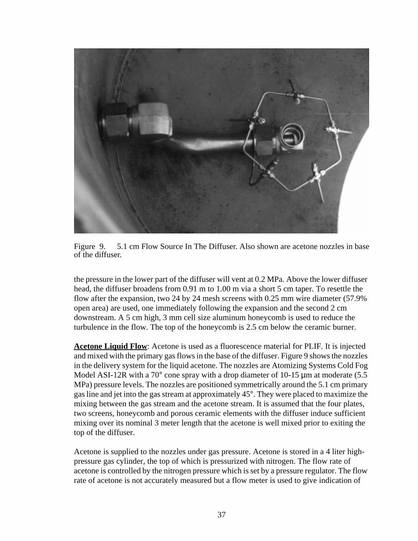
the pressure in the lower part of the diffuser will vent at 0.2 MPa. Above the lower diffuser head, the diffuser broadens from 0.91 m to 1.00 m via a short 5 cm taper. To resettle the flow after the expansion, two 24 by 24 mesh screens with 0.25 mm wire diameter (57.9% open area) are used, one immediately following the expansion and the second 2 cm downstream. A 5 cm high, 3 mm cell size aluminum honeycomb is used to reduce the turbulence in the flow. The top of the honeycomb is 2.5 cm below the ceramic burner.
Acetone Liquid Flow: Acetone is used as a fluorescence material for PLIF. It is injected and mixed with the primary gas flows in the base of the diffuser. Figure 9 shows the nozzles in the delivery system for the liquid acetone. The nozzles are Atomizing Systems Cold Fog Model ASI-12R with a 70° cone spray with a drop diameter of 10-15 µm at moderate (5.5 MPa) pressure levels. The nozzles are positioned symmetrically around the 5.1 cm primary gas line and jet into the gas stream at approximately 45°. They were placed to maximize the mixing between the gas stream and the acetone stream. It is assumed that the four plates, two screens, honeycomb and porous ceramic elements with the diffuser induce sufficient mixing over its nominal 3 meter length that the acetone is well mixed prior to exiting the top of the diffuser.
Acetone is supplied to the nozzles under gas pressure. Acetone is stored in a 4 liter high-pressure gas cylinder, the top of which is pressurized with nitrogen. The flow rate of acetone is controlled by the nitrogen pressure which is set by a pressure regulator. The flow rate of acetone is not accurately measured but a flow meter is used to give indication of
Figure 9. 5.1 cm Flow Source In The Diffuser. Also shown are acetone nozzles in baseof the diffuser.
37

flow. The gas manifold to supply the nitrogen has the requisite manual and pressure relief valves to meet safety requirements.
Particle Flow: PIV seed particles are injected into both the ambient air stream and the plume. Part of the development experiments was to design the seeders to produce a uniform density of seed in the flow. As such the seeder hardware and its placement changed as the
Figure 10. Flow Broadening Plates In Lower Diffuser.
38

ore d. In .
ground m two e laser . The
while while
s, xtend d to a mm
rticle der the length a 13 otated
n of rials
is a me is
a
the ately
ligned opane
test series progressed. The description below is the configuration of the seeders for the tests selected for data analysis.
With one exception, the basic seeder design is a 13 mm inner diameter (16 mm O. D.) tube with a 10 mm slot cut axially along one side. The slot is covered with an 80 mesh screen. The tube is loaded with the particles and then shaken with a vibrator to induce the particles to exit via the screen. The screen functions to ‘declump’ the particles to provide a muniform seed particle size distribution. Both pneumatic and electric vibrators were trieneither case was gas supplied to the tubes themselves. Only particles were injected
For the air stream, Figure 6 and Figure 7 show the location of the seeders above the plane. The seeders are made from four 0.5 m long tubes suspended from chains frosupports. Four tubes are used, spaced 7.6 cm apart with the inner tubes straddling thsheet. The tubes are slanted with the height of the outer radius being fixed at 0.66 mheight of the inner radius varied with the test. For helium tests the height was 0.20 m,for reacting tests it was 0.15 m. Also for the helium test the slots were rotated down, for the reacting tests they were rotated to face inward toward the laser sheet.
The supports for the ambient seeders are 6 mm thick by 5.1 cm wide steel flat strapaligned to minimize the disturbance to the flow. The supports are 1.04 m high and eto a radius 0.52 m from the center of the plume. The pneumatic vibrators are mountebar supporting the particle laden tubes as far from the plume flow as possible, and 6diameter gas lines are used for gas supply and return.
The particle injectors for the plume stream are located a few centimeters below the honeycomb flow straightener (-0.18 m below the ground plane) in the diffuser. The pasupply tubes are aligned with the laser sheet. Three tubes are used, one directly unlaser sheet and one 7.6 cm on either side. The slots in each tube extend for the entireof the tube within the diffuser. The center tube is thinner than the other seeders. It ismm O. D. tube with a 6 mm slot cut along one side. For all tests the central seeder is rdown, but for the reacting tests the side seeders were rotated inward 45° from the horizontal. Electric vibrators are used to shake the tubes to disperse the seed.
Ignitor Gas Flow: For the reacting flow experiments, it is necessary to ensure ignitiothe flammable materials as they enter the facility. An accumulation of flammable matewould result in an explosion. To ensure ignition, a powerful flame source is used. It Manchester Model 8017 hand burner capable of throwing a 1.2 m long flame. The flacontrollable so that it is turned on only to ignite the fuels and then is turned off after ignition. The ignitor has a small pilot flame the remains lit at all times. It is nominallycentimeter in diameter and 5 cm long.
As shown in Figure 11, the ignitor is mounted under the ground plane with the tip ofburner at ground level at the edge of the plume source. The tip is angled at approxim45° to the vertical so that the flame can penetrate the burner diameter. The ignitor is awith the 270° angle, so that it is perpendicular to the laser sheet. The burner runs on pr
39

and is supplied by a separate gas manifold. The gas manifold has the requisite manual and pressure relief valves to meet safety requirements.
Figure 11. Ignitor.
40

Air SourceThe numerical simulation of the flow patterns within the FLAME facility resulted in large changes in the manner in which air was distributed in the facility. To achieve the desired radial inflow, it was necessary to introduce the air symmetrically into the facility. Since air enters the walls at only four 0.61 m square openings at the base of the east and west walls in the north and south corners, substantial duct work had to be created. In the resultant design, the duct work channels the air so that it enters the central chamber with only a vertical velocity component from an annular surface with an inner diameter of 2.30 m and an outer diameter of 2.91 m. The top surface of the air source is located 1.74 m below the ground plane, 0.71 m above the facility floor. The annulus is fabricated from sixteen 45° segments, four to each quadrant of the facility. The segments are not rounded but flat on each side so as to be easy to fabricate and yet adequately approximate an annulus.
While the facility can be operated in a free draw mode, four fans with a maximum capacity of 4.7 m3/sec (10,000 scfm) each can also supply air to the facility. The surface area of the annular air source is 9.84 m2, resulting in a maximum velocity of 1.9 m/s. The fans are infinitely variable between zero and their maximum value so that the air inlet velocity can be adjusted.
The numerical simulations indicated that as long as the flow rate from the air ducts is less than a critical value for a given plume flow, a trapped vortex will form beneath the ground plane. The vortex will stay trapped below the plane of the plume and radial inflow into the plume will result. If the air flow rate is too high, the top of the trapped vortex will climb above the plane of the plume and a region of downflow will occur along the plume. This downflow results in a fairly complex flow pattern in which counterflow exists along the sides of the plume except at its base where the solid lip forces radial inflow at the base. Hence, the flow rate of the air needs to be adjusted below a set value for each plume flow in order for radial inflow to result in the facility.
The numerical simulations also showed that the air velocities were sufficiently high at the surface of the air ducts that radial inflow was not possible in the square FLAME facility without providing overall radial symmetry to an elevation just above the surface of the burner. Therefore, sixteen 0.61 mm thick, 3.05 m tall, steel sheets were hung vertically on unistrut frames such that they provided the cylindrical shield wall shown (cutaway) in Figure 4. These sheets prevent corner flows from disrupting the radial symmetry. The base of the sheets begin in the air ducts 0.30 m above the floor (an elevation of -2.15 m) and run to an elevation of 0.90 m. The sheets can be seen in the background in Figure 7.
To facilitate air flow from the air inlets in the four corners of the FLAME facility to the annular air vent, the entire area between the cylindrical shield wall and square FLAME facility walls has been turned into an air duct. Essentially, a false floor has been created 0.79 m above the facility floor (1.61 m below the ground plane). Baffles are used to channel the air between the false floor and the facility floor from the four corners into the annular vents. Six baffles are used in each quadrant, four to the vertices of the four segments making up the annulus and two additional baffles to subdivide the middle segments.
41
The air flow from the corners of the FLAME facility must flow under the shield wall (0.30 m above the floor vs. 0.79 m to the false floor between the cylindrical shield wall that the FLAME walls) to reach the air ducts. In a manner similar to the gas plume diffuser, the air ducts have horizontally mounted plates and screens are used to create a uniform flow exiting the top of the ducts. Two plates, two screens, and a honeycomb are used. The lowest plate is mounted above the lower edge of the shield wall, at 0.51 m above the floor. In 5 cm increments, the next plate, two screens and the 0.5 cm high honeycomb are mounted. The plates have a fixed blockage ratio of approximately 0.5, with the lower one having 2.5 cm holes and the upper one having 1.3 cm holes. The screens are 24 by 24 mesh with a 0.25 mm wire diameter yielding a 57.9% open area. The aluminum honeycomb has 3 mm cells.
Chimney ExhaustThe only outlet of the facility is through the chimney. The square chimney has insulation mats on the inside faces and remains nominally 2.3 m on each side throughout its height except at the exit. The chimney height is nominally 7.32 m. At the exit, the north and south faces taper inward at nominally 45 degree angles to leave a 1.2 m (4 ft) by 2.4 m (8 ft) opening at the exit. Nominal 1.2m (4 ft) long by 2.4 m (8 ft) doors, hinged on the east and west side, open outward at nominally 135 degrees from the exit plane during a test.
The chimney is deliberately obstructed by pipes throughout its length. The pipes induce mixing in the duct channel while the flow is still hot. The additional mixing, partially oxidizes the soot (smoke) from the fire in the central chamber. Because of the pipes, the chimney is not as efficient as it could be in drafting. However, the pipes provide some buffering between the central chamber and the exit, so that slight changes in air pressure at the exit due to light breezes are not directly felt within the central chamber.
Diagnostics
PIV Diagnostics
There are five major steps needed for measuring two-dimensional velocity fields using PIV, each of which must be optimized to achieve the best measurement accuracy:
1. Illuminating the flow field so that sufficient light is scattered by seed particles. Illumination is usually by a laser light sheet, with wavelength and pulse separation appropriate to the flow conditions,
2. Seeding the flow with appropriate tracer seed particle,
3. Recording multiple-exposure or sequential photographs of the scattered light field,
4. Processing and/or digitizing the photographs,
5. Measuring the velocity field by extracting velocity vectors throughout the illuminated plane.
42
The illumination source for this PIV system is a pair of pulsed XeCl excimer lasers: aLambda-Physik LPX 150 oscillator and a Lambda-Physik LPX 220 amplifier. The maxi-mum pulse repetition frequency is 200 Hz. The maximum pulse energy is 400 mJ at the 308nm wavelength. The UV wavelength was chosen to allow optical filtering of the PIV signal,i.e. UV light scattered by the seed particles can be recorded while visible light is blocked.Use of a quartz UV Nikkor lens allowed the 308 nm light to be collected. The full opticalsetup included turning mirrors to get the laser beam from the laser trailer into the FLAMEfacility and directed toward the plume inlet, and light sheet optics, including a sphericallens (7500 mm focal length) and a cylindrical lens (75 mm focal length to give the 1 m highsheet typically used). The light sheet thickness was about 6 mm. Thinner light sheets weretested, but gave inferior PIV performance due to 3D motion sweeping particles out of thethinner light sheets. Other optics used for development tests including a 3000 mm focallength spherical lens that gave a narrower light sheet with its waist above the burner, andseveral different cylindrical lenses, including 700 mm focal length to give a 7.5 cm highsheet, and a 200 mm focal length to give a 0.5 m high light sheet.
PIV images were recorded on 30.5 m rolls of Kodak T-Max ASA 400 35 mm black and white motion picture film. T-Max film has a wide exposure latitude, extremely fine grained resolution, and good UV sensitivity. A 255-355 nm bandpass filter was used to eliminate visible light from the UV image, both to eliminate room light coming in the chimney and, more importantly, to eliminate the visible flame emission in the reacting cases. The cameras were 35 mm pin-registered PhotoSonics 4ML motion picture cameras, running at a nominal 180 frames/s frame rate. The PIV and PLIF cameras were mounted side-by-side for all tests. The cameras viewed the plume through a large front surface mirror, as shown in Fig. 1.
The cameras were synchronized together, and controlled the excimer laser pulses. Synchronization was achieved for about 1000 frames per test. The cameras require upwards of five seconds to accelerate, stabilize, and synchronize at the nominal 180 frames/s frame rate. At that speed, the cameras have approximately 8 seconds of total run time for the 30.5 m film length. Hence, about 3 seconds of run time, or approximately 550 frames, are available for analysis. For a puffing frequency of 1.5 per second, between 4 and 5 puffs can be captured for analysis.
The seed particles selected for this application were glass microballoons (3M Scotchlite K1), with a mean particle diameter of 70 µm and a density of 0.125 g/cc. The characteristic particle response time (τ=ρpdp
2/18µ, see Friedlander, 1977) was about 2 msec for air at 20 C, and improved for warmer air due to its higher viscosity. The large particle size was necessitated by the large image size. The choice of glass instead of lower density plastic (as low as 0.03 g/cc, e.g., Nobel 091DE80) was due to the simultaneous PIV and PLIF. The plastic microballoons fluoresced under UV excitation, with a fluorescent emission in the range of expected acetone fluorescence. It was also hoped that the glass particles would withstand higher temperatures before disintegrating but, as will be shown below, significant loss of seed particles still occurred in the flame zones. Seeders were located both in the plume inlet and in the entrained air, just outside of plume (see Figure 6). All seeding was performed by pre-loading particles into 1.25 cm ID stainless steel tubes, into which
43

lling each rs on
N), wn in
he cribed it was r the
beam trum is
xcite
ith a lens ne
0.95 cm slots had been milled along the length of the tube, then covered with 80 mesh stainless steel screen. An electronic or pneumatic ball vibrator was then attached to the particle-filled tubes. Three seed tubes were placed in the plume, one on centerline and two on either side. Four seed tubes were hung on chains in the entrained air on either side of the plume inlet, set up to span the light sheet (see Figure 6). To initiate seeding, just before starting the PIV data acquisition, the vibrators were started, shaking particles out through the screen regions along the full tube length. This worked fairly well in the main gas plume, where the particles were swept into the buoyant plume. However, placement of the seed tubes in the entrained air was more difficult, and required adjustment for each gas tested, since each had different entrainment velocity.
The 35 mm motion picture film images (picture size 25 mm wide by 19 mm high) were digitized at high resolution using a Kodak RFS3570 film scanner with 2150 dpi optical resolution. A fully automated film scanning station was developed, using a stepper motor to pull the roll film through the film scanner. All digitization was controlled by a LabView program (National Instruments) developed for this application. This program controls a 25000 step-per-revolution stepper motor to pull the film through the scanner, activates the TWAIN scanning module, scans the negative, stores the scanned image, then repeats the process an arbitrary number of times. The scanned 35 mm black and white images were stored as 3 Mbyte files on CD’s. Because of camera vibrations and inaccuracy in puexactly one frame through the scanner, the images had to be manually registered toother prior to PIV analysis. This was done by selecting an area of interest with cornewell-defined objects in the field. This manual step added ± 2 pixels uncertainty to the analysis.
PIV analysis was performed using the Insight-NT software (V. 1.22, TSI, St. Paul, Mrunning on a Pentium Pro computer under Windows NT 4.0. For the vector fields shothis report, a 96 by 96 pixel interrogation region was used. The scaling is 677µm/pixel.
Acetone: Laser-induced fluorescence of acetone was used as a tracer for the fuel. Tacetone was seeded directly into the fuel flow using an atomizer nozzle system desin a previous section of this report. Maximum acetone seed levels at the fuel nozzle exmaintained below 2 percent to meet safety requirements. The ultraviolet laser light foexcitation of the acetone molecule was provided by the same 308-nm excimer laserused to illuminate particles for the PIV measurements. The acetone absorption speccontinuous over the wavelength range of 240 to 320 nm, with the peak excitation wavelength at 275 nm. Thus, the 308 nm wavelength of the excimer laser used to efluorescence from the acetone is to the long side of the peak excitation wavelength,resulting in about a factor of four reduction in absorption cross section. The acetonefluorescence emission spectrum is broadband, extending from 350 to 550 nm. The fluorescence signal was detected using an identical 35 mm pin-registered camera wstandard 105 mm focal length, f/1.2 glass lens to collect the visible signal. The glasseffectively eliminated scattered UV light from the laser so that only the desired acetofluorescence signal was recorded.
44
Initial excitation of the acetone molecule at 308 nm results in excitation to the singlet state. Strong coupling between this singlet state and the first triplet system quickly results in an excited-state population distribution consisting of a mixed singlet-triplet character, from which the fluorescence is rapidly emitted. As discussed by Clemens and Paul (1995), the acetone fluorescence signal is largely independent of its collisional environment. Thus the fluorescence signal is directly proportional to the acetone number density. As a result, in the nonreacting isothermal helium plume, the acetone fluorescence signal is directly proportional to the mole fraction, while in the reacting H2 and CH4 flows where temperature variations are large, the fluorescence signal is proportional to number density. An additional problem with the use of acetone as a fuel tracer in reacting flows is that since it rapidly pyrolizes at temperatures above 1200K, acetone will not survive in the high temperature flame zone, and will also likely disappear when mixed with hot combustion products. Thus the acetone images are useful to identify the vortical structure and location in the reacting flows, but do not provide a quantitative representation of fuel concentration in regions where the temperature is high.
Cameras: Scientific 35 mm movie cameras and standard video were used to record the images for the tests. The standard video was used primarily for conduct of operations. Even though digital images are required for PIV, Photosonics 4ML 35 mm movie cameras were chosen for PIV and fluorescence imaging over newer digital CCD cameras because of speed and resolution requirements. At the time of these experiments, digital cameras that can match 35 mm film resolution (~2000 x 1500 pixels) cannot record faster than about an image per second. Digital cameras that can match the Photosonics 4ML recording speed of 200 frames/sec, typically have less than standard video resolution (~540 x 460 pixels). Therefore, the Photosonics 4ML 35 mm film cameras were chosen to record the scientific data. The analog-to-digital conversion to permit PIV analysis was performed post-test with the Kodak RFS3570 scanner already discussed. It is expected that digital cameras will eventually replace film, however, on-the-fly analog-to-digital conversion is still not fast enough to permit the data density required for the current tests.
The 4ML cameras, shown in Figure 7, are pin-registered which permits better frame-to-frame correlation than rotating mirror cameras; thus enhancing data reduction by reducing frame-to-frame jitter. Typically two cameras were used in each test. One camera was used to record images in the UV while the other was used to record visible light images. Simultaneity was required between the laser pulses and the camera images being in frame. Since the cameras are analog devices, it was a challenge to synchronize both cameras and the laser at the typical frame rate of 180 frames/sec used during the tests. Development activity to achieve this synchronization reliably consumed a number of tests. However, reliable synchronization was achieved for upwards of 1000 frames per test for the data tests presented in this report.
Frequency separation between the UV images and visible light images was achieved through lensing and filters. For the UV image, a quartz Nikon 105 mm fixed focal length lens with a minimum f-stop of 4.5 was used. A quartz lens was used since glass will not pass UV light. The fixed focal length Nikon is the only 35 mm format UV lens known to the authors. A 255-355 nm band pass optical filter centered on the laser wavelength of 308
45
nm was used to eliminate visible light from the image. For the visible light image, a glass Nikon 105 mm fixed focal length lens with a minimum f-stop of 1.2 was used. The glass in the lens prevented scattered UV light from being recorded by the camera. Most tests were conducted without filters, allowing the full visible spectrum to be recorded. The exceptions are for hydrogen flame tests and selected methane flame tests, a high pass optical filter was used to block wavelengths longer than 550 nm (to strip off the yellow from soot radiation).
The cameras were mounted side by side for all tests. Because of the fixed focal length UV lens, it was necessary to change the position of the cameras to change the field of view. Initially, the cameras were placed at a distance of approximately 3.6 meters from the centerline of the plume to have an image area of approximately 0.66 meter horizontal by 0.5 meter high. The image area focussed on the edge of the burner to the centerline of the burner horizontally and from the surface of the burner to approximately one burner radius high. The cameras were placed perpendicular to the path of the laser, but at an elevation slightly above the centerline of the light sheet. By tilting the cameras down slightly, this placement permitted imaging the front lip of the burner simultaneously with the light sheet. As a result the view is foreshortened slightly, but clearly shows that the light sheet intersects the center of the burner.
Later (from Test #22 on) the cameras were repositioned with a path length of approximately 6.1 meters to have an image area of approximately 1.2 meters horizontal by slightly less than a meter high. A straight line path of over about 4 meters is not possible in the 6 m square FLAME facility. Therefore, a mirror was used to create the required path length. To accommodate the UV light, an approximately 0.6 meter high and 1 meter wide metallized front surface mirror was used. The mirror was place in the position originally occupied by the cameras for Tests #1 - 21. The cameras were repositioned down below the surface of the burner just outside of the diffuser as shown in Figure 7. The camera position relative to the burner surface can also be seen in Figure 6 in which the camera images are visible in the mirror.
With one exception, PIV images were recorded on black and white Kodak T-Max ASA 400 film. T-Max film has a wide exposure latitude and extremely fine grained resolution (100 line pairs per millimeter). Experience has shown that it has good UV sensitivity. It is also easily processed at most photo labs. The film was special ordered from Kodak in 30.5 m rolls with cores to match the Photosonics cameras. The 30.5 m rolls were used for all tests but Test #51. The cameras can also support 61 m and 122 m rolls, the latter of which was used for Test #51.
The shorter length was chosen for these development tests as a compromise between cost and duration. The cameras require upwards of five seconds to come to 180 frames/sec and synchronize. At that speed, the cameras have approximately 8 seconds of total run time. Hence, about 3 seconds of run time, or approximately 540 frames are available for analysis. For an expected puffing frequency of 1.5 per second, between 4 and 5 puffs can be captured for analysis. For the maximum film load of 122 m, upwards of 4000 frames can be available for analysis, with upward of 30 puffs captured. Hence it is possible to capture a statistically significant number of the slowest mode eddies with the current cameras.
46

The visible images were recorded with different films depending on the tests. For attempts to image acetone fluorescence, Kodak T-Max ASA 400 film, was used. For hydrogen tests, both black and white Kodak T-Max ASA 400 film and color Kodak VND ASA 160 film was tried. For the methane tests, color Kodak VND ASA 160 film was used.
In addition to the movie cameras, video cameras were used to record the overall flow within the facility during each test. The video was primarily to assist in the conduct of the tests to verify that the ignitor and particle seeders were functioning appropriately, and that the flame went out during the purge operations. One camera was located between the Photosonic 4ML cameras so that the operators could view what the 35 mm cameras were imaging. The second camera was located on the inside of the east door of the facility about 1/2 meter below the rim of the burner. It used a wide angle lens to view from just below the burner to the entrance of the chimney and a good portion of the internals horizontally. These videos were also useful for overall flow visualization, e.g., for determining puffing frequencies.
Boundary Condition DiagnosticsFor each inlet, outlet and boundary, an attempt is made to measure important mass, momentum, and energy boundary conditions. The state of technology is such that measurement of all variables at all boundaries are not possible. Further, for each variable measured, there are economic limits on the spatial and temporal resolution that can be achieved. The choices reflected below represent the authors attempt to balance measurement fidelity and cost.
A summary of the boundary condition measurements is given in Table 1 and Table 2. Table 1 gives the measurement location, uncertainty in the location measurement, device type, and serial number, if available. Table 2 gives the device measurement range, uncertainty in the range, and response time of the gage.
TABLE 1. Boundary Condition Gage Locations
Measurement Type
MeasurementLocation* (r m, θ°, z m)
Uncertainty in Measured Location (∆r m, ∆θ°, ∆z m)
Manufacture & Model Number
Gage Serial Number
Ambient
Humidity 3.85 , 93, -1.92 0.05, 1, 0.05 Omega RH411 ----
Velocity 2.60, 11, -1.69 0.03, 1, 0.03 Accusense AVS-1012 ----
Velocity 2.60, 34, -1.69 0.03, 1, 0.03 Accusense AVS-1012 ----
Velocity 2.60, 56, -1.69 0.03, 1, 0.03 Accusense AVS-1012 ----
Velocity 2.60, 79, -1.69 0.03, 1, 0.03 Accusense AVS-1012 ----
Velocity 2.60, 101, -1.69 0.03, 1, 0.03 Accusense AVS-1012 ----
Velocity 2.60, 124, -1.69 0.03, 1, 0.03 Accusense AVS-1012 ----
Velocity 2.60, 146, -1.69 0.03, 1, 0.03 Accusense AVS-1012 ----
Velocity 2.60, 169, -1.69 0.03, 1, 0.03 Accusense AVS-1012 ----
47
Velocity 2.60, 191, -1.69 0.03, 1, 0.03 Accusense AVS-1012 ----
Velocity 2.60, 214, -1.69 0.03, 1, 0.03 Accusense AVS-1012 ----
Velocity 2.60, 236, -1.69 0.03, 1, 0.03 Accusense AVS-1012 ----
Velocity 2.60, 259, -1.69 0.03, 1, 0.03 Accusense AVS-1012 ----
Velocity 2.60, 281, -1.69 0.03, 1, 0.03 Accusense AVS-1012 ----
Velocity 2.60, 304, -1.69 0.03, 1, 0.03 Accusense AVS-1012 ----
Velocity 2.60, 326, -1.69 0.03, 1, 0.03 Accusense AVS-1012 ----
Velocity 2.60, 349, -1.69 0.03, 1, 0.03 Accusense AVS-1012 ----
Absolute Pres-sure
External, z=-1.69 --, --, 0.05 Setra 470 703306
Diff. pressure 2.63, 123, -1.66Pabsolute
0.03, 1, 0.03 Setra 264 688888
Diff. pressure 2.55, 34, -1.662.55, 349, -1.66
0.03, 1, 0.03 Setra 264 708028
Diff. pressure 2.55, 79, -1.662.55, 34, -1.66
0.03, 1, 0.03 Setra 264 688891
Diff. pressure 2.55, 124 -1.662.55, 79, -1.66
0.03, 1, 0.03 Setra 264 708033
Diff. pressure 2.55, 169, -1.662.55, 124, -1.66
0.03, 1, 0.03 Setra 264 68887
Diff. pressure 2.55, 214, -1.662.55, 169, -1.66
0.03, 1, 0.03 Setra 264 688882
Diff. pressure 2.55, 259, -1.662.55, 214, -1.66
0.03, 1, 0.03 Setra 264 688883
Diff. pressure 2.55, 304, -1.662.55, 259, -1.66
0.03, 1, 0.03 Setra 264 708035
Diff. pressure 2.55, 349, -1.662.55, 304, -1.66
0.03, 1, 0.03 Setra 264 708034
Temperature 3.85, 93°, -1.92 0.05, 1, 0.05 Gordon Type K, 1.6mm, ungrounded
----
Plume
Diluent flow rate
In high pressure manifold
------- FlowMetrics 16M50 9703TM3059/2A
In high pressure manifold
------- Hedland 771.090 9621
Diluent line temperature
In high pressure manifold
------- Gordon Type K, 1.6mm, ungrounded
----
Diluent line pressure
In high pressure manifold
------- Endevco 8530B-200 10108
TABLE 1. Boundary Condition Gage Locations
Measurement Type
MeasurementLocation* (r m, θ°, z m)
Uncertainty in Measured Location (∆r m, ∆θ°, ∆z m)
Manufacture & Model Number
Gage Serial Number
48

Fuel flow rate In high pressure manifold
------- FlowMetrics 16M50 9703TM3059/1A
In high pressure manifold
------- Hedland 771.090 9620
Fuel line tem-perature
In high pressure manifold
------- Gordon Type K, 1.6mm, ungrounded
----
Fuel line pres-sure
In high pressure manifold
------- Endevco 8530B-200 10136
Diff pressure 0.47, 193, 0.0Pabsolute
0.01, 1, 0.003 Setra 264 708027
Diff pressure 0.47, 193, 0.00.47, 193, 0.97
0.01, 1, 0.03 Setra 264 581731
Temperature - Diffuser
0.0, 90, -0.05 0.03, 180, 0.03 Gordon Type K, 1.6mm, ungrounded
----
Outflow
Dyn. pressure 0.00, 90, 4.56 0.03, 180, 0.05 SNL Bi-Directional V 708030
Dyn. pressure 0.27, 90, 4.56 0.03, 6, 0.05 SNL Bi-Directional V 708031
Dyn. pressure 0.53, 90, 4.56 0.03, 3, 0.05 SNL Bi-Directional V 708014
Dyn. pressure 0.80, 90, 4.56 0.03, 2, 0.05 SNL Bi-Directional V 708012
Dyn. pressure 1.06, 90, 4.56 0.03, 2, 0.05 SNL Bi-Directional V 708010
Dyn. pressure 1.33, 90, 4.56 0.03, 2, 0.05 SNL Bi-Directional V 708008
Dyn. pressure 0.8, 180, 4.56 0.03, 2, 0.05 SNL Bi-Directional V 708016
Dyn. pressure 0.8, 270, 4.56 0.03, 2, 0.05 SNL Bi-Directional V 708005
Dyn. pressure 0.8, 0, 4.56 0.03, 2, 0.05 SNL Bi-Directional V 708006
Diff. pressure 2.63, 123, -1.660.04, 90, 4.56
0.03, 1, 0.030.03, 180, 0.05
Setra 264 708032
Diff pressure 0.31, 90, 4.560.04, 90, 4.56
0.03, 6, 0.050.03, 180, 0.05
Setra 264 708015
Diff pressure 0.57, 90, 4.560.31, 90, 4.56
0.03, 3, 0.050.03, 6, 0.05
Setra 264 708013
Diff pressure 0.84, 90, 4.560.57, 90, 4.56
0.03, 2, 0.050.03, 3, 0.05
Setra 264 708011
Diff pressure 1.10, 90, 4.560.84, 90, 4.56
0.03, 2, 0.050.03, 2, 0.05
Setra 264 708009
Diff pressure 1.37, 90, 4.561.10, 90, 4.56
0.03, 2, 0.050.03, 2, 0.05
Setra 264 708007
Diff pressure 0.72, 198, 10.0Pabsolute
0.05, 4, 0.1--, --, 0.05
Setra 264 688890
TABLE 1. Boundary Condition Gage Locations
Measurement Type
MeasurementLocation* (r m, θ°, z m)
Uncertainty in Measured Location (∆r m, ∆θ°, ∆z m)
Manufacture & Model Number
Gage Serial Number
49
Temperature 0.04, 180, 4.56 0.03, 180, 0.05 Gordon Type K, 1.6mm, ungrounded
----
Temperature 0.31, 98, 4.56 0.03, 6, 0.05 Gordon Type K, 1.6mm, ungrounded
----
Temperature 0.57, 94, 4.56 0.03, 3, 0.05 Gordon Type K, 1.6mm, ungrounded
----
Temperature 0.84, 93, 4.56 0.03, 2, 0.05 Gordon Type K, 1.6mm, ungrounded
----
Temperature 1.10, 92, 4.56 0.03, 2, 0.05 Gordon Type K, 1.6mm, ungrounded
----
Temperature 1.37, 92, 4.56 0.03, 2, 0.05 Gordon Type K, 1.6mm, ungrounded
----
Temperature 0.84, 180, 4.56 0.03, 2, 0.05 Gordon Type K, 1.6mm, ungrounded
----
Temperature 0.84, 270, 4.56 0.03, 2, 0.05 Gordon Type K, 1.6mm, ungrounded
----
Temperature 0.84, 0, 4.56 0.03, 2, 0.05 Gordon Type K, 1.6mm, ungrounded
----
Solid Surface
Temperature - Ground
0.53, 135, 0.0 0.01, 2, 0.003 Gordon Type K, 1.6mm, ungrounded
----
Temperature - Ground
0.74, 135, 0.0 0.01, 2, 0.003 Gordon Type K, 1.6mm, ungrounded
----
Temperature - Ground
0.97, 135, 0.0 0.01, 1, 0.003 Gordon Type K, 1.6mm, ungrounded
----
Temperature - Cyl. Shield
2.91, 141, -1.49 0.03, 1, 0.03 Gordon Type K, 1.6mm, ungrounded
----
Temperature - Cyl. Shield
2.91, 141, -0.32 0.03, 1, 0.03 Gordon Type K, 1.6mm, ungrounded
----
Temperature - Cyl. Shield
2.91, 141, 0.84 0.03, 1, 0.03 Gordon Type K, 1.6mm, ungrounded
----
Temperature - Wall
3.05, 132, 1.64 0.05, 1, 0.05 Gordon Type K, 1.6mm, ungrounded
----
Temperature - Vert. Shield
2.95, 132, 3.01 0.05, 1, 0.05 Gordon Type K, 1.6mm, ungrounded
----
Temperature - Slant Shield
2.29, 132, 3.91 0.05, 1, 0.05 Gordon Type K, 1.6mm, ungrounded
----
Temperature -Slant Shield
1.81, 132, 4.28 0.05, 2, 0.05 Gordon Type K, 1.6mm, ungrounded
----
TABLE 1. Boundary Condition Gage Locations
Measurement Type
MeasurementLocation* (r m, θ°, z m)
Uncertainty in Measured Location (∆r m, ∆θ°, ∆z m)
Manufacture & Model Number
Gage Serial Number
50
*Second location is given for differential pressure measurements and represents low pressure tap.
TABLE 2. Measurement Ranges, Uncertainty, and Response Time
Measurement Type
MeasurementLocation (r m, θ°, z m)
Measurement Range
Measurement Uncertainty
Response Time (ms)
Ambient
Humidity 3.85 , 93, -1.92 2-98% RH +/- 3% 30,000
Velocity 2.60, 11, -1.69 0.18 - 3.5 m/s +/- 0.18 m/s 100
Velocity 2.60, 34, -1.69 0.07 - 1.4 m/s +/- 0.07 m/s 100
Velocity 2.60, 56, -1.69 0.18 - 3.5 m/s +/- 0.18 m/s 100
Velocity 2.60, 79, -1.69 0.07 - 1.4 m/s +/- 0.07 m/s 100
Velocity 2.60, 101, -1.69 0.18 - 3.5 m/s +/- 0.18 m/s 100
Velocity 2.60, 124, -1.69 0.07 - 1.4 m/s +/- 0.07 m/s 100
Velocity 2.60, 146, -1.69 0.18 - 3.5 m/s +/- 0.18 m/s 100
Velocity 2.60, 169, -1.69 0.07 - 1.4 m/s +/- 0.07 m/s 100
Velocity 2.60, 191, -1.69 0.18 - 3.5 m/s +/- 0.18 m/s 100
Velocity 2.60, 214, -1.69 0.07 - 1.4 m/s +/- 0.07 m/s 100
Velocity 2.60, 236, -1.69 0.18 - 3.5 m/s +/- 0.18 m/s 100
Velocity 2.60, 259, -1.69 0.07 - 1.4 m/s +/- 0.07 m/s 100
Velocity 2.60, 281, -1.69 0.18 - 3.5 m/s +/- 0.18 m/s 100
Velocity 2.60, 304, -1.69 0.07 - 1.4 m/s +/- 0.07 m/s 100
Velocity 2.60, 326, -1.69 0.18 - 3.5 m/s +/- 0.18 m/s 100
Velocity 2.60, 349, -1.69 0.07 - 1.4 m/s +/- 0.07 m/s 100
Absolute Pres-sure
External, z = -1.69 m
600 - 1100 mbar +/- 0.2 mbar One reading per test
Diff. pressure 2.63, 123, -1.66Pabsolute
0 - 25 N/m2 +/- 1.7 Pa 50
Diff. pressure 2.55, 34, -1.662.55, 349, -1.66
0 - 25 N/m2 +/- 1.7 Pa 50
Diff. pressure 2.55, 79, -1.662.55, 34, -1.66
0 - 25 N/m2 +/- 1.7 Pa 50
Diff. pressure 2.55, 124 -1.662.55, 79, -1.66
0 - 25 N/m2 +/- 1.7 Pa 50
Diff. pressure 2.55, 169, -1.662.55, 124, -1.66
0 - 25 N/m2 +/- 1.7 Pa 50
Diff. pressure 2.55, 214, -1.662.55, 169, -1.66
0 - 25 N/m2 +/- 1.7 Pa 50
Diff. pressure 2.55, 259, -1.662.55, 214, -1.66
0 - 25 N/m2 +/- 1.7 Pa 50
51
Diff. pressure 2.55, 304, -1.662.55, 259, -1.66
0 - 25 N/m2 +/- 1.7 Pa 50
Diff. pressure 2.55, 349, -1.662.55, 304, -1.66
0 - 25 N/m2 +/- 1.7 Pa 50
Temperature 3.85, 93°, -1.92 73 - 1523°K MAX (1.1°K or 0.4% of reading)
4,200
Plume
Diluent flow rate
Flowmetrics in high pressure manifold
High: 0 - 24 l/s +/- 0.12 l/s 25
Hedland in high pressure manifold
Low: 4.7 -42 l/s std*
+/- 1 l/s std 1000
Diluent line temperature
In high pressure manifold
73 - 1523°K MAX (1.1°K or 0.4% of reading)
4,200
Diluent line pressure
In high pressure manifold
0 - 1.4 MPa +/- 7 kPa 0.015
Fuel flow rate Flowmetrics in high pressure manifold
High: 0 - 24 l/s +/- 0.12 l/s 25
Hedland in high pressure manifold
Low: 4.7 -42 l/s std*
+/- 1 l/s std 1000
Fuel line tem-perature
In high pressure manifold
73 - 1523°K MAX (1.1°K or 0.4% of reading)
4,200
Fuel line pres-sure
In high pressure manifold
0 - 1.4 MPa +/- 7kPa 0.015
Diff pressure 0.47, 193, 0.0Pabsolute
0 - 25 N/m2 +/- 1.7 Pa 50
Diff pressure 0.47, 193, 0.00.47, 193, 0.97
0 - 25 N/m2 +/- 1.7 Pa 50
Temperature - Diffuser
0.0, 90, -0.05 73 - 1523°K MAX (1.1°K or 0.4%of reading)
4,200
Outflow
Dyn. pressure 0.00, 90, 4.56 0 - 25 N/m2 +/- 2.0 (kg/s2/m) 50
Dyn. pressure 0.27, 90, 4.56 0 - 25 N/m2 +/- 2.0 (kg/s2/m) 50
Dyn. pressure 0.53, 90, 4.56 0 - 25 N/m2 +/- 2.0 (kg/s2/m) 50
Dyn. pressure 0.80, 90, 4.56 0 - 25 N/m2 +/- 2.0 (kg/s2/m) 50
Dyn. pressure 1.06, 90, 4.56 0 - 25 N/m2 +/- 2.0 (kg/s2/m) 50
Dyn. pressure 1.33, 90, 4.56 0 - 25 N/m2 +/- 2.0 (kg/s2/m) 50
Dyn. pressure 0.8, 180, 4.56 0 - 25 N/m2 +/- 2.0 (kg/s2/m) 50
Dyn. pressure 0.8, 270, 4.56 0 - 25 N/m2 +/- 2.0 (kg/s2/m) 50
Dyn. pressure 0.8, 0, 4.56 0 - 25 N/m2 +/- 2.0 (kg/s2/m) 50
TABLE 2. Measurement Ranges, Uncertainty, and Response Time
Measurement Type
MeasurementLocation (r m, θ°, z m)
Measurement Range
Measurement Uncertainty
Response Time (ms)
52
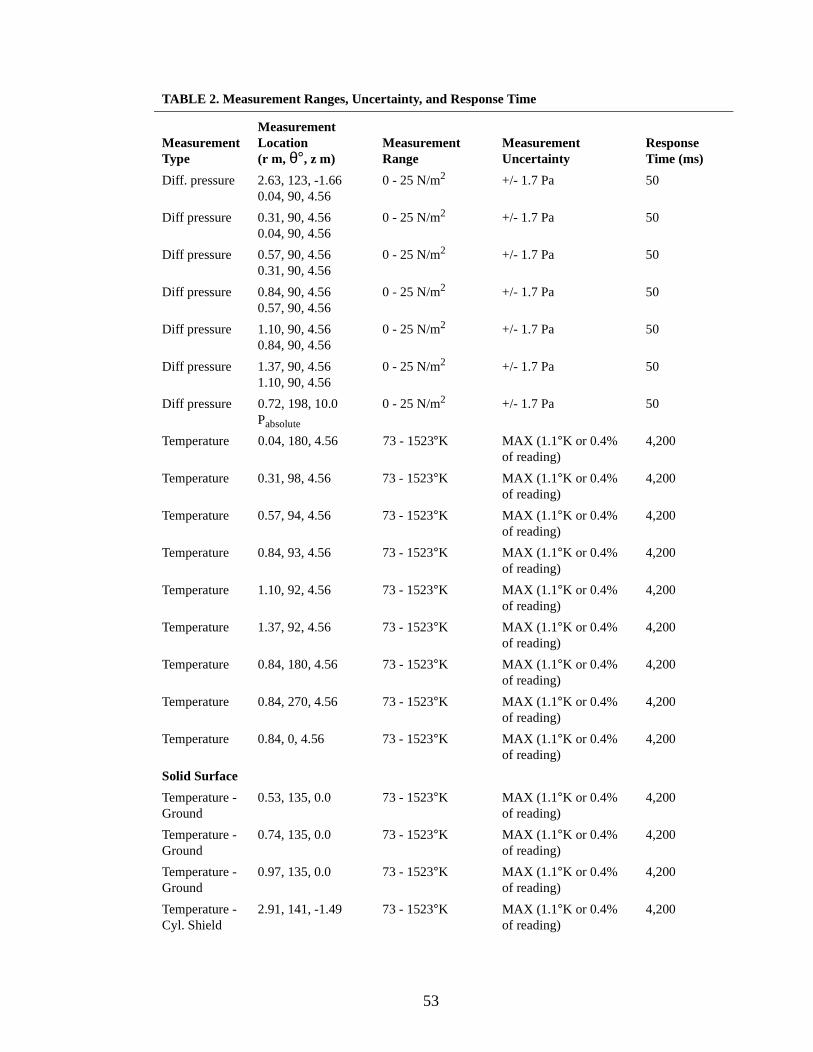
Diff. pressure 2.63, 123, -1.660.04, 90, 4.56
0 - 25 N/m2 +/- 1.7 Pa 50
Diff pressure 0.31, 90, 4.560.04, 90, 4.56
0 - 25 N/m2 +/- 1.7 Pa 50
Diff pressure 0.57, 90, 4.560.31, 90, 4.56
0 - 25 N/m2 +/- 1.7 Pa 50
Diff pressure 0.84, 90, 4.560.57, 90, 4.56
0 - 25 N/m2 +/- 1.7 Pa 50
Diff pressure 1.10, 90, 4.560.84, 90, 4.56
0 - 25 N/m2 +/- 1.7 Pa 50
Diff pressure 1.37, 90, 4.561.10, 90, 4.56
0 - 25 N/m2 +/- 1.7 Pa 50
Diff pressure 0.72, 198, 10.0Pabsolute
0 - 25 N/m2 +/- 1.7 Pa 50
Temperature 0.04, 180, 4.56 73 - 1523°K MAX (1.1°K or 0.4% of reading)
4,200
Temperature 0.31, 98, 4.56 73 - 1523°K MAX (1.1°K or 0.4% of reading)
4,200
Temperature 0.57, 94, 4.56 73 - 1523°K MAX (1.1°K or 0.4% of reading)
4,200
Temperature 0.84, 93, 4.56 73 - 1523°K MAX (1.1°K or 0.4% of reading)
4,200
Temperature 1.10, 92, 4.56 73 - 1523°K MAX (1.1°K or 0.4% of reading)
4,200
Temperature 1.37, 92, 4.56 73 - 1523°K MAX (1.1°K or 0.4% of reading)
4,200
Temperature 0.84, 180, 4.56 73 - 1523°K MAX (1.1°K or 0.4% of reading)
4,200
Temperature 0.84, 270, 4.56 73 - 1523°K MAX (1.1°K or 0.4% of reading)
4,200
Temperature 0.84, 0, 4.56 73 - 1523°K MAX (1.1°K or 0.4% of reading)
4,200
Solid Surface
Temperature - Ground
0.53, 135, 0.0 73 - 1523°K MAX (1.1°K or 0.4% of reading)
4,200
Temperature - Ground
0.74, 135, 0.0 73 - 1523°K MAX (1.1°K or 0.4% of reading)
4,200
Temperature - Ground
0.97, 135, 0.0 73 - 1523°K MAX (1.1°K or 0.4% of reading)
4,200
Temperature - Cyl. Shield
2.91, 141, -1.49 73 - 1523°K MAX (1.1°K or 0.4% of reading)
4,200
TABLE 2. Measurement Ranges, Uncertainty, and Response Time
Measurement Type
MeasurementLocation (r m, θ°, z m)
Measurement Range
Measurement Uncertainty
Response Time (ms)
53
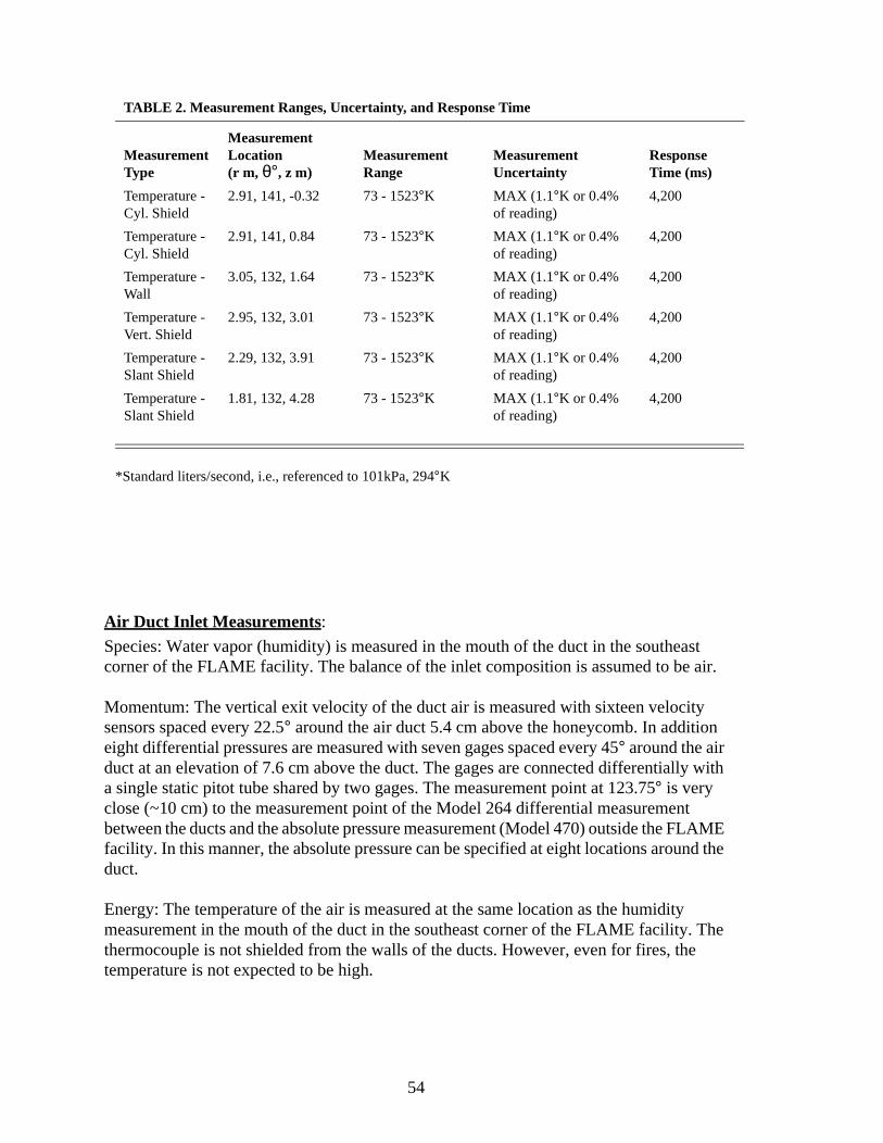
Air Duct Inlet Measurements:
Species: Water vapor (humidity) is measured in the mouth of the duct in the southeast corner of the FLAME facility. The balance of the inlet composition is assumed to be air.
Momentum: The vertical exit velocity of the duct air is measured with sixteen velocity sensors spaced every 22.5° around the air duct 5.4 cm above the honeycomb. In addition eight differential pressures are measured with seven gages spaced every 45° around the air duct at an elevation of 7.6 cm above the duct. The gages are connected differentially with a single static pitot tube shared by two gages. The measurement point at 123.75° is very close (~10 cm) to the measurement point of the Model 264 differential measurement between the ducts and the absolute pressure measurement (Model 470) outside the FLAME facility. In this manner, the absolute pressure can be specified at eight locations around the duct.
Energy: The temperature of the air is measured at the same location as the humidity measurement in the mouth of the duct in the southeast corner of the FLAME facility. The thermocouple is not shielded from the walls of the ducts. However, even for fires, the temperature is not expected to be high.
Temperature - Cyl. Shield
2.91, 141, -0.32 73 - 1523°K MAX (1.1°K or 0.4% of reading)
4,200
Temperature - Cyl. Shield
2.91, 141, 0.84 73 - 1523°K MAX (1.1°K or 0.4% of reading)
4,200
Temperature - Wall
3.05, 132, 1.64 73 - 1523°K MAX (1.1°K or 0.4% of reading)
4,200
Temperature - Vert. Shield
2.95, 132, 3.01 73 - 1523°K MAX (1.1°K or 0.4% of reading)
4,200
Temperature - Slant Shield
2.29, 132, 3.91 73 - 1523°K MAX (1.1°K or 0.4% of reading)
4,200
Temperature -Slant Shield
1.81, 132, 4.28 73 - 1523°K MAX (1.1°K or 0.4% of reading)
4,200
*Standard liters/second, i.e., referenced to 101kPa, 294°K
TABLE 2. Measurement Ranges, Uncertainty, and Response Time
Measurement Type
MeasurementLocation (r m, θ°, z m)
Measurement Range
Measurement Uncertainty
Response Time (ms)
54

Plume Inlet Measurements:
Species: The composition of the plume is determined by the relative mass flow rates in the two main gas lines leading into the diffuser. Three measurements are required in each line to specify the mass flow rate for each species. In each line a high and low range velocity, temperature, and absolute pressure measurement is made.
The flow rate of seed particles (and acetone on selected tests) are not rigorously measured for each test. However, estimates can be made from total volume measurements before and after each test and the duration that the flow was on. Each flow is anticipated to have a secondary effect on the plume. For example the maximum flow rate of acetone, below the flammability limit, is about 2% of the helium flow in which it was used.
Momentum: The plume exit velocity is measured by the PIV diagnostics since the laser sheet passes over the surface of the plume for each test. In addition, the static pressure is measured with a combination of a differential pressure measurements leading back to the absolute pressure measurement outside the facility.
Energy: The temperature measurement is made just below the ceramic plate. The thermocouple is not shielded from the diffuser walls or ceramic plate. However, the ceramic plate provides shielding from the thermal flux for the reacting flow cases.
FLAME Outflow Measurements:
Species: Due to the temperature of the exit flow in the reacting flow cases, no species measurements were made in the exit flow. Hence the density at the exit cannot be quantitatively specified.
Momentum: The momentum, ρv2, at the exit of the central chamber where it joins the chimney was measured with Sandia designed bi-directional pitot tubes. The pitot tubes are made from Inconel to survive the exhaust temperatures. The design and calibration details can be found in Kent and Schneider, 1987. Nine measurements are made. In addition the static pressure is also measured at the six locations along the same radius at 90°. Differential pressure measurements are also made that lead back to the absolute pressure reading outside the facility and further up near the exit of the exhaust stack.
Energy: Exhaust gas temperature is measured at nine locations at the exit of the central chamber where it joins the chimney. The thermocouples are mounted 0.04 m from each of the bi-directional velocity probes directly opposing the static pressure measurements. The thermocouples are not shielded and can see the relatively cool walls as well as the hot flame for the reacting flow cases. The thermocouples could be shielded so that their viewfactors are limited to the hot flame below the thermocouples and the cooler chimney exhaust. However, they are in close proximity to the momentum measurements and it was decided that the shielding may interfere with the flow.
55

data/orders to the
ever, t from n, and se was he take t be ed an ime
Solid Boundaries Measurements:
Species: No measurements are required or taken because the walls are solid.
Momentum: No measurements are required or taken because the walls are solid, so a no-slip boundary condition exists.
Energy: For non-reacting flow cases, the central chamber is isothermal, and no energy measurements are required. However, for reacting flow cases, thermal radiation heats the surrounding surfaces. To account for thermal radiation, surfaces with large view factors with respect to the fire were instrumented with thermocouples. Ten total thermocouple measurements were made for each test. Due to the expected radial symmetry of the plume, all measurements were made along a single radius at a nominal 135° angle.
Obviously, ten measurements represents a small number of measurement points given the large surface area of the FLAME facility. Cost was a determining factor. Hence, the data is sufficient for boundary conditions, but is not sufficient for validation of the thermal radiation solver.
The thermocouples are held in contact with the solid surface with a 6 mm wide, 75 µm thick, Nichrome strip that is spot welded to the surface. The thermocouple junction is pinned under the strip parallel to the surface. Since the junctions of the thermocouples are not grounded to the sheath, the junctions are actually 0.8 mm off the surface. Prior to mounting the thermocouple, the surfaces are ground to remove scale and ensure good contact.
Data Acquisition System For Boundary Condition Measurements:
Three types of transient data recorders are used to record the data for the tests, two CAMAC style systems, the LeCroy 6810’s and BiRa 5908’s, and one Hewlett-Packard 3582 controller device. The system is controlled by a personal computer. The transient recrecord data to volatile memory during the test. After the test the data is downloaded inpersonal computer. Including two timing channels (start and laser pulse), the data acquisition system recorded 72 channels per test.
Timing of the data acquisition system varied as the test program was developed. Howthe data acquisition, laser pulse, and camera frame were all in synchronization. Outputhe controlling camera, used to trigger the laser, was recorded on the data acquisitioused as a clock for the majority of channels. For those channels in which the laser pulused as a clock, the data correspond to an exact frame on the film. In this manner, tboundary condition data can be closely correlated with the PIV and PLIF images. Toadvantage of this close correlation, the triggering of the data acquisition system muscorrelated with the film. This was done on later tests by recording a signal that producoptical fiducial mark on the film. On the earliest tests, timing was from camera start.However, this did not prove satisfactory since it was difficult to tell the camera start t
56

from the film images. Typically, 800 to 1000 images were captured with the cameras at speed. Hence, there is a like number of samples recorded for each channel.
Details of the data acquisition system are given in Table 3.
TABLE 3. Data Acquisition Parameters
Measurement Type
MeasurementLocation (r m, θ°, z m)
DAS HardwareDigitizer/Slot/Channel
Bits Per Instrument Range
Frequency(samples/sec)
Timing
Film fiducial ------ LeCroy 6810/3/2 2048 100,000
Laser pulse timing
------ LeCroy 6810/3/1 2048 100,000
Ambient
Humidity 3.85 , 93, -1.92 LeCroy6810/7/1 2048 laser pulsed*
Velocity 2.60, 11, -1.69 BiRa5908/8/2 1024 laser pulsed
Velocity 2.60, 34, -1.69 BiRa5908/8/1 1024 laser pulsed
Velocity 2.60, 56, -1.69 BiRa5908/8/16 1024 laser pulsed
Velocity 2.60, 79, -1.69 BiRa5908/8/15 1024 laser pulsed
Velocity 2.60, 101, -1.69 BiRa5908/8/14 1024 laser pulsed
Velocity 2.60, 124, -1.69 BiRa5908/8/13 1024 laser pulsed
Velocity 2.60, 146, -1.69 BiRa5908/8/12 1024 laser pulsed
Velocity 2.60, 169, -1.69 BiRa5908/8/11 1024 laser pulsed
Velocity 2.60, 191, -1.69 BiRa5908/8/10 1024 laser pulsed
Velocity 2.60, 214, -1.69 BiRa5908/8/9 1024 laser pulsed
Velocity 2.60, 236, -1.69 BiRa5908/8/8 1024 laser pulsed
Velocity 2.60, 259, -1.69 BiRa5908/8/7 1024 laser pulsed
Velocity 2.60, 281, -1.69 BiRa5908/8/6 1024 laser pulsed
Velocity 2.60, 304, -1.69 BiRa5908/8/5 1024 laser pulsed
Velocity 2.60, 326, -1.69 BiRa5908/8/4 1024 laser pulsed
Velocity 2.60, 349, -1.69 BiRa5908/8/3 1024 laser pulsed
Absolute
Pressure
External to FLAME, z = -1.69 m
Computer/RS232 >4096 One reading per test
Diff. pressure 2.63, 123, -1.66Pabsolute
BiRa5908/3/1 1024 laser pulsed
Diff. pressure 2.55, 34, -1.662.55, 349, -1.66
BiRa5908/13/8 1024 laser pulsed
Diff. pressure 2.55, 79, -1.662.55, 34, -1.66
BiRa5908/13/15 1024 laser pulsed
57

Diff. pressure 2.55, 124 -1.662.55, 79, -1.66
BiRa5908/13/14 1024 laser pulsed
Diff. pressure 2.55, 169, -1.662.55, 124, -1.66
BiRa5908/13/13 1024 laser pulsed
Diff. pressure 2.55, 214, -1.662.55, 169, -1.66
BiRa5908/13/12 1024 laser pulsed
Diff. pressure 2.55, 259, -1.662.55, 214, -1.66
BiRa5908/13/11 1024 laser pulsed
Diff. pressure 2.55, 304, -1.662.55, 259, -1.66
BiRa/908/13/10 1024 laser pulsed
Diff. pressure 2.55, 349, -1.662.55, 304, -1.66
BiRa5908/13/9 1024 laser pulsed
Temperature 3.85, 93°, -1.92 HP3582//10
Plume
Diluent flow rate
In high pressure manifold
LeCroy6810/7/3 2048 laser pulsed
Diluent line temperature
In high pressure manifold
HP3582//21 4096 1.1
Diluent line pressure
In high pressure manifold
LeCroy6810/11/2 2048 10,000
Fuel flow rate In high pressure manifold
LeCroy6810/7/4 2048 laser pulsed
Fuel line tem-perature
In high pressure manifold
HP3582//22 4096 1.1
Fuel line pres-sure
In high pressure manifold
LeCroy6810/11/3 2048 10,000
Diff pressure 0.47, 193, 0.0Pabsolute
BiRa5908/13/5 1024 laser pulsed
Diff pressure 0.47, 193, 0.00.47, 193, 0.97
BiRa5908/13/6 1024 laser pulsed
Temperature - Diffuser
0.0, 90, -0.05 HP3582//23 4096 1.1
Outflow
Dyn. pressure 0.00, 90, 4.56 BiRa5908/3/3 1024 laser pulsed
Dyn. pressure 0.27, 90, 4.56 BiRa5908/3/4 1024 laser pulsed
Dyn. pressure 0.53, 90, 4.56 BiRa5908/3/5 1024 laser pulsed
Dyn. pressure 0.80, 90, 4.56 BiRa5908/3/6 1024 laser pulsed
Dyn. pressure 1.06, 90, 4.56 BiRa5908/3/7 1024 laser pulsed
Dyn. pressure 1.33, 90, 4.56 BiRa5908/3/8 1024 laser pulsed
Dyn. pressure 0.8, 180, 4.56 BiRa5908/3/9 1024 laser pulsed
TABLE 3. Data Acquisition Parameters
Measurement Type
MeasurementLocation (r m, θ°, z m)
DAS HardwareDigitizer/Slot/Channel
Bits Per Instrument Range
Frequency(samples/sec)
58

Dyn. pressure 0.8, 270, 4.56 BiRa5908/3/10 1024 laser pulsed
Dyn. pressure 0.8, 0, 4.56 BiRa5908/3/11 1024 laser pulsed
Diff. pressure 2.63, 123, -1.660.04, 90, 4.56
BiRa5908/3/2 1024 laser pulsed
Diff pressure 0.31, 90, 4.560.04, 90, 4.56
BiRa5908/3/12 1024 laser pulsed
Diff pressure 0.57, 90, 4.560.31, 90, 4.56
BiRa5908/3/13 1024 laser pulsed
Diff pressure 0.84, 90, 4.560.57, 90, 4.56
BiRa5908/3/14 1024 laser pulsed
Diff pressure 1.10, 90, 4.560.84, 90, 4.56
BiRa5908/3/15 1024 laser pulsed
Diff pressure 1.37, 90, 4.561.10, 90, 4.56
BiRa5908/3/16 1024 laser pulsed
Diff pressure 0.72, 198, 10.0Pabsolute
BiRa5908/13/7 1024 laser pulsed
Temperature 0.04, 180, 4.56 HP3582//7 4096 1.1
Temperature 0.31, 98, 4.56 HP3582//6 4096 1.1
Temperature 0.57, 94, 4.56 HP3582//5 4096 1.1
Temperature 0.84, 93, 4.56 HP3582//4 4096 1.1
Temperature 1.10, 92, 4.56 HP3582//3 4096 1.1
Temperature 1.37, 92, 4.56 HP3582//2 4096 1.1
Temperature 0.84, 180, 4.56 HP3582//8 4096 1.1
Temperature 0.84, 270, 4.56 HP3582//9 4096 1.1
Temperature 0.84, 0, 4.56 HP3582//1 4096 1.1
Solid Surface
Temperature - Ground
0.53, 135, 0.0 HP3582//13 4096 1.1
Temperature - Ground
0.74, 135, 0.0 HP3582//12 4096 1.1
Temperature - Ground
0.97, 135, 0.0 HP3582//11 4096 1.1
Temperature - Cyl. Shield
2.91, 141, -1.49 HP3582//14 4096 1.1
Temperature - Cyl. Shield
2.91, 141, -0.32 HP3582//15 4096 1.1
Temperature - Cyl. Shield
2.91, 141, 0.84 HP3582//16 4096 1.1
Temperature - Wall
3.05, 132, 1.64 HP3582//20 4096 1.1
TABLE 3. Data Acquisition Parameters
Measurement Type
MeasurementLocation (r m, θ°, z m)
DAS HardwareDigitizer/Slot/Channel
Bits Per Instrument Range
Frequency(samples/sec)
59
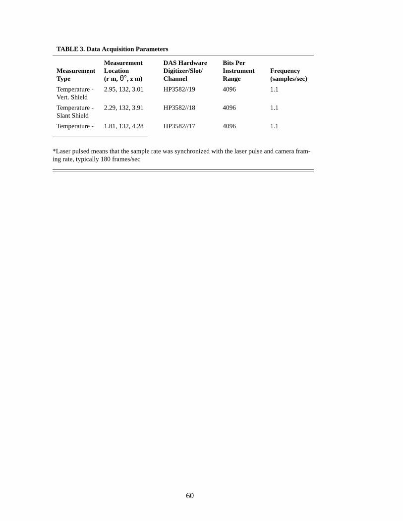
Temperature - Vert. Shield
2.95, 132, 3.01 HP3582//19 4096 1.1
Temperature - Slant Shield
2.29, 132, 3.91 HP3582//18 4096 1.1
Temperature -Slant Shield
1.81, 132, 4.28 HP3582//17 4096 1.1
*Laser pulsed means that the sample rate was synchronized with the laser pulse and camera fram-ing rate, typically 180 frames/sec
TABLE 3. Data Acquisition Parameters
Measurement Type
MeasurementLocation (r m, θ°, z m)
DAS HardwareDigitizer/Slot/Channel
Bits Per Instrument Range
Frequency(samples/sec)
60
Test Methods/Matrix
Test Procedure
In general, test methods were refined as part of the development program and therefore varied test to test. The general procedures for tests selected for data analysis will be described below for helium and generically for reacting flow (hydrogen & methane).
Non-Reacting Test
In general, several subsystems had to be brought into a state of readiness prior to a test, including the gas supply for the plume, the air supply for the air vents, the particle seeders, the laser, the cameras, and the data acquisition system for the boundary conditions.
Prior to the test for the gas supply system, typically six gas bottles, would be loaded into the diluent side of the bottle farm and the nitrogen supply used to control the remote pneumatic valves and seeders would be checked and replaced if necessary. The valving on the gas manifolds would be brought to a safe state prior to opening any of the bottles. For non-reacting tests without acetone, there are three subsystems in the gas manifold. The first to be brought on line is the control subsystem which provides nitrogen to pneumatic control valves. The second is the main gas supply to the plume, and the third is the nitrogen supply to run the seeders during a test. In general, the procedure is to supply gas to each system with a final valve closed until it is necessary to flow gas. Gas is supplied by opening the bottle(s) in the gas manifold and then setting the pressure regulator to the desired pressure. For control nitrogen, the setting is nominally 70 psi. For the gas supply to the plume, the setting is nominally 200 psi, and for the seeders, the setting is nominally 160 psi. The flow control valve on the main gas supply to the plume is electric and is powered up and the percent opening is set to achieve the desired flow rate. Opening of the final valve for the nitrogen control is done during setup to allow for control of the pneumatic valves. Opening the final valve on the main gas supply system initiates the test. Opening of the final valve on the seeders occurs only after the gas supply has been flowing for typically 40 seconds, and just prior to the start of the laser, cameras, and data acquisition.
Prior to the test for the air vents, the vent panels on the FLAME facility exhaust stack are opened to allow ventilation of the central chamber. The air supply fans are powered up, set to the desired air flow rate at the air duct, and the settings recorded. The fans are typically powered up and left running for several hours prior to the test because they are stable and allow for ventilation of the facility. Typically, the front doors are closed several minutes before the test so that the air flow patterns in the FLAME facility due to the air flow stabilize prior to beginning the gas flow to the plume.
61
Prior to the test for the seeders, particles are loaded into the seeders. New particles are loaded for each test to avoid clumping brought on by moisture. The seeders are mounted in their respective locations and the pneumatic or electric vibrators attached. The vibrators are not activated until the plume flow has been flowing for typically 40 seconds.
Prior to the test for the laser system, it is powered up within its trailer for at least a half hour before the test and run at a low repetition rate of typically 1 pulse/sec. The laser is aligned, beam quality is adjusted, and power is recorded. Since the beam travels through open air before entering the FLAME facility, signage and personnel control are established before allowing the beam to leave the trailer. The beam is then aligned over the plume source so that it just grazes the ceramic surface and passes through the plume centerline. The laser is then put on external control to allow the camera pulse to fire it.
Prior to the test for the cameras, focus, alignment, and function are checked for two video cameras and the 35 mm movie camera. A UV band pass filter is placed on the quartz lens on the movie camera to filter out visible light. The movie camera controls timing for the entire test. Most of the data acquisition channels take their timing from this camera as does the laser. Just prior to loading film, a system wide timing check is done to verify that all timing hardware works. Film is then loaded into the movie camera.
Prior to the test for the boundary condition diagnostics, power supplies for the pressure transducers in the gas manifold, the differential pressure measurements, humidity meter and the velocity measurements are turned on. The output of the pressure transducers in the gas manifold are supply voltage dependent so the voltage is recorded. The flow meter range (high or low) is selected on the main gas supply to the plume. The data acquisition system is powered on and the digitizer settings entered. Function of the external clock pulse and trigger from the camera is checked.
At the initiation of the test, an absolute pressure measurement is made to establish ambient pressure. The video recorders are turned on and the flow is begun in the plume by opening the final shut-off valve in the gas manifold. Typically about 30 seconds are permitted to pass while the flow establishes itself in the facility. Steady flow at the plume source is determined by monitoring the flow rate, temperature, and pressure in the main gas line. A 10 second countdown sequencer is then triggered. At t-2 seconds, the cameras are triggered to start. Manually, the seeder vibrators are started at the same time. At time zero, the data acquisition system is triggered. Between five and six seconds of film are recorded at nominally 180 frames/sec before the test is complete.
Reacting Test
In addition to the procedures described for the non-reacting test, additional procedures and equipment are required to conduct a reacting flow test. The additions to, and differences between, the non-reacting tests are described below.
For the gas supply system, there are significant procedural changes and an additional gas subsystem has to brought on line. Unignited flammable gas cannot be allowed in the
62
presence of air either in the plume diffuser or in the FLAME facility itself. Therefore to run a flammable test, the diluent line must be used prior to, and after, the fuel line to purge the gas system of air. Therefore, both the fuel and diluent bottle farms are loaded with typically six gas bottles. Prior to introducing fuel into the fuel lines, the diluent gas is routed through the fuel system lines to ensure that no air is present when fuel is introduced. This purging is required since the operation is manned and high pressure hydrogen/air mixtures require very little ignition energy.
Purging of the diffuser takes longer and is done just prior to initiating fuel flow. Oxygen sampling within the diffuser has shown that two volume changes within the diffuser will produce and oxygen concentration below the flammability limit for a range of flow rates. This volume corresponds to just over half of a full gas bottle, so at least one full bottle is expended on purging before and after the test. Purging is done over one to two minutes before and after the fuel has been flowed.
In order to ensure that flammable fuels do not accumulate in the FLAME facility, an ignitor is used. Prior to flowing gas in the main gas lines to the plume, the ignitor is made operational. The ignitor system is propane based and the pressure regulator is set at 50 psi. A striker is used to ignite the pilot light on the ignitor at the start of propane flow. The pilot remains lit during the entire test. The ignitor is capable of throwing a flame across the plume source and is used only at the start of fuel flow until a flame is established, and during post-test purge while fuel is being purged from the system.
Typically two 35 mm movie cameras are used in a flammable test. The second camera is slaved to the first camera so that it synchronizes with the first. Typically, the first camera has the UV band pass filter on the quartz lens while the second camera is set up to record visible light images and uses a glass lens. For methane tests, it has either no filter while for hydrogen tests it has a high frequency pass at 550 nm.
At the initiation of the test, the diffuser is purged and the ignitor is turned on. Fuel flow is then started and the ignitor turned off after the flame is established (usually only a few seconds). Otherwise the test proceeds as in the non-reacting case except the flow rates in the reacting flow cases are typically lower than that for helium. Therefore, more time, typically around one minute, is allowed for the flow to reach steady state within the FLAME facility.
At the end of the test, purging of the diffuser and fuel lines occurs to ensure that all fuel is vented from the system. The ignitor is turned on during purging of the fuel lines.
Diagnostic Development Tests
Table 4 lists all tests and identifies lessons learned. The first dozen tests were to ring out the hardware and conduct basic functionality checks. In the interests of rapid development, design problems identified during this time were not fixed immediately. Rather, the functionality for both non-reacting and reacting flows were tested. Safety issues prevented
63
one ders ut it , just
cities lium r inlet ers.
ation s/sec. ior to ty of
sed for d in the g t as e tests rlier
hs for ource re is off. being ed by
the use of acetone until later in the series and boundary condition diagnostics had not been fully implemented. The first successful recording of 1/2 m by 2/3 m UV image of the base of the methane flame occurred with Test #12. However, the particle image velocimetry software was unable to process the image due to lack of correlation of particle images between frames. It was decided that the 1 mm sheet thickness was too thin and particles were leaving the plane of the laser too quickly.
The light sheet was thickened to 6 mm with Test #14 by changing from a 3000 mm to a 7500 mm focal length spherical lens in the light sheet forming optics. The thicker light sheet proved to be sufficient for PIV measurements. The camera speed was increased to 180 frames/sec beginning with Test #21. The camera were repositioned to acquire approximately a 0.8 m by 1.2 m view to capture the full base of the fire beginning with Test #22. Boundary condition diagnostics were installed and the data acquisition system brought on line in Test #27. The acetone plumbing was installed and safety issues addressed by Test #29.
The majority of effort for test numbers in the 30’s was to alter the particle seeders inmanner or another to improve the seed density and uniformity in the image. The seewere modified in virtually every test. Significant progress was made in image quality btook a number of tests to realize that the seeders were not the cause of the problemresponding to the problem. During these tests, it became clear that the air inlet velohad been set too high in previous tests. This resulted in a down flow of air for the hetests and up flow of air for the reacting flow tests. Attempts were made to adjust the aiflow rates to produce better flow patterns in combination with positioning of the seed
However, a number of tests in the 30’s were marred by repeated camera synchronizproblems. The cameras are analog devices and had difficulty synching at 180 frameThe problem was intermittent with the camera’s synching on systems checks just prthe run, but not on the run itself. Significant effort was applied to increase the reliabilithe camera synching electronics.
With the seeding and camera problems under control, tests in the 40’s range were uacquiring PIV data. The best of these tests were chosen for analysis to be discussenext section. The air flow rate to the air ducts for these tests was set by the remaininAccusense gauges which proved to be unreliable. Therefore, the air velocity was nouniform as it could have been and the imbalance was noticeable on the late methanin particular. The fires were not as uniformly symmetric as had been observed in eatests. However, in general the runs were good.
The final test was used to study a natural fluorescence image in the blue wavelengthydrogen tests. The fluorescent image was recorded on earlier tests, however, its swas not clear. Therefore, in the final test, a long run was conducted in which the twoparameters (laser and seed particles) were varied on and off. Hence, four states westudied. Laser and particles on, laser and particles off, land either on while the otherThe fluorescence only occurred with the particles on, and was invariant to the laser on. Therefore, it was determined that the fluorescence is natural and not being induc
64

the laser, and that it is coming from the decomposition of the borosilicate glass particles. To conduct this test longer 122 m film rolls were used. The test lasted 24 seconds instead of the usual 5 to 6 seconds for the 30.5 m film rolls.
TABLE 4. Development Test Log
Test Plume AcetoneCamera Setup
Lens/Filter/FilmDAS
Working
1 He No UV//Tmax No
2 He No UV//Tmax No
3 He No UV//Tmax No
4 He No UV//Tmax No
5 He No UV//Tmax No
6 H2 No UV//Tmax No
7 CH4 No UV/255-355/Tmax No
8 CH4 No UV/255-355/Tmax No
9 H2 No UV/255-355/Tmax No
10 He No UV/255-355/Tmax No
11 H2 No UV/255-355/Tmax No
12 CH4 No UV/255-355/Tmax, Vis//Tmax
No
13 H2 No UV/255-355/Tmax No
14 He No UV/255-355/Tmax No
15 He No UV/255-355/Tmax No
16 He No UV/255-355/Tmax No
17 He No UV/255-355/Tmax No
18 He No UV/255-355/Tmax No
19 He No UV/255-355/Tmax No
20 He No UV/255-355/Tmax No
21 He No UV/255-355/Tmax No
22 CH4 No UV/255-355/Tmax, Vis//Clr
No
65

23 CH4 No UV/255-355/Tmax, Vis//Clr
No
24 He No UV/255-355/Tmax No
25 He No UV/255-355/Tmax No
26 He No UV/255-355/Tmax No
27 He No UV/255-355/Tmax, Vis//Tmax
Yes
28 H2 Yes UV/255-355/Tmax, Vis//Tmax
Yes
29 H2 Yes UV/255-355/Tmax, Vis/-550/Tmax
Yes
30 He Yes UV/255-355/Tmax, Vis//Tmax
No
31 CH4 No UV/255-355/Tmax, Vis/-550/Clr
Yes
32 H2 Yes UV/255-355/Tmax, Vis/-500&-550/Tmax
Yes
33 He No UV/255-355/Tmax Yes
34 He Yes UV/255-355/Tmax, Vis//Tmax
Yes
35 H2/He Yes UV/255-355/Tmax, Vis/-550/Clr
Yes
36 H2 No UV/255-355/Tmax, Vis/-500/Tmax
Yes
37 H2 No UV//Tmax, Vis/550/Tmax
Yes
38 CH4 No UV/255-355/Tmax, UV//Clr
Yes
39 He No UV/255-355/Tmax No
40 CH4 No UV/255-355/Tmax, UV/-550/Clr
Yes
41 10%CH4/ 90%He
No UV/255-355/Tmax, UV/-550/Clr
No
42 He No UV/255-355/Tmax Yes
TABLE 4. Development Test Log
Test Plume AcetoneCamera Setup
Lens/Filter/FilmDAS
Working
66
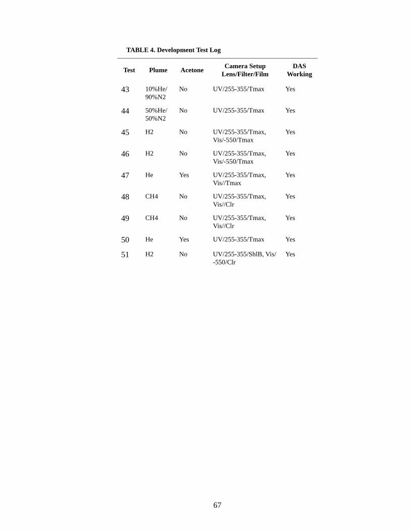
43 10%He/90%N2
No UV/255-355/Tmax Yes
44 50%He/50%N2
No UV/255-355/Tmax Yes
45 H2 No UV/255-355/Tmax, Vis/-550/Tmax
Yes
46 H2 No UV/255-355/Tmax, Vis/-550/Tmax
Yes
47 He Yes UV/255-355/Tmax, Vis//Tmax
Yes
48 CH4 No UV/255-355/Tmax, Vis//Clr
Yes
49 CH4 No UV/255-355/Tmax, Vis//Clr
Yes
50 He Yes UV/255-355/Tmax Yes
51 H2 No UV/255-355/ShlB, Vis/-550/Clr
Yes
TABLE 4. Development Test Log
Test Plume AcetoneCamera Setup
Lens/Filter/FilmDAS
Working
67

68
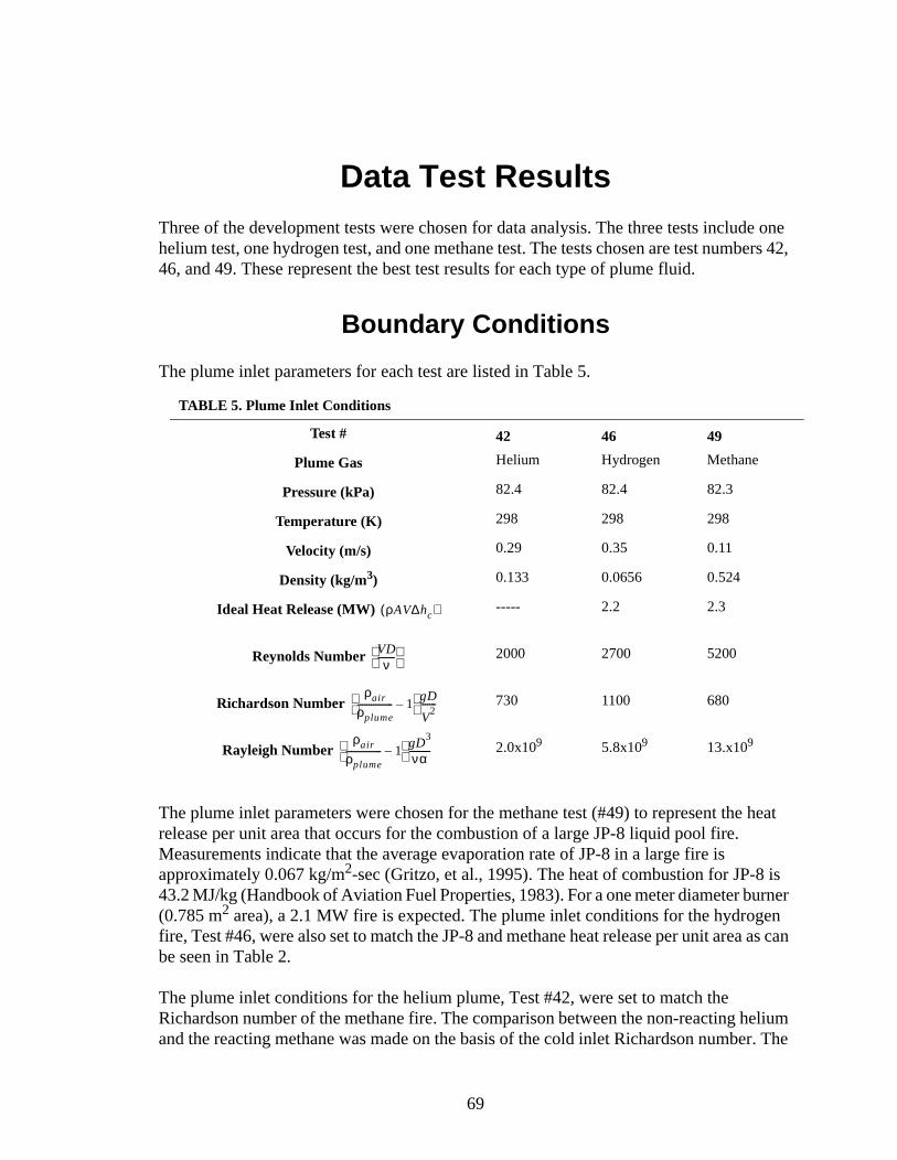
Data Test ResultsThree of the development tests were chosen for data analysis. The three tests include one helium test, one hydrogen test, and one methane test. The tests chosen are test numbers 42, 46, and 49. These represent the best test results for each type of plume fluid.
Boundary Conditions
The plume inlet parameters for each test are listed in Table 5.
The plume inlet parameters were chosen for the methane test (#49) to represent the heat release per unit area that occurs for the combustion of a large JP-8 liquid pool fire. Measurements indicate that the average evaporation rate of JP-8 in a large fire is approximately 0.067 kg/m2-sec (Gritzo, et al., 1995). The heat of combustion for JP-8 is 43.2 MJ/kg (Handbook of Aviation Fuel Properties, 1983). For a one meter diameter burner (0.785 m2 area), a 2.1 MW fire is expected. The plume inlet conditions for the hydrogen fire, Test #46, were also set to match the JP-8 and methane heat release per unit area as can be seen in Table 2.
The plume inlet conditions for the helium plume, Test #42, were set to match the Richardson number of the methane fire. The comparison between the non-reacting helium and the reacting methane was made on the basis of the cold inlet Richardson number. The
TABLE 5. Plume Inlet Conditions
Test # 42 46 49
Plume Gas Helium Hydrogen Methane
Pressure (kPa) 82.4 82.4 82.3
Temperature (K) 298 298 298
Velocity (m/s) 0.29 0.35 0.11
Density (kg/m3) 0.133 0.0656 0.524
Ideal Heat Release (MW) ----- 2.2 2.3
Reynolds Number 2000 2700 5200
Richardson Number 730 1100 680
Rayleigh Number 2.0x10⁹ 5.8x10⁹ 13.x109
ρAV∆hc( )
VDν
--------
ρair
ρplume---------------- 1–
gD
V2
-------
ρair
ρplume---------------- 1–
gD3
να----------
69

Richardson number was chosen because it represents the ratio of buoyant to momentum forces at the base of the plume. It can also be thought of as representing the ratio of baroclinic vorticity generation to shear vorticity generation.
The boundary conditions for each of the three tests are given in Table 6. While substantial effort was made to acquire sufficient boundary condition information to be able to use the data generated for validation purposes, the overall performance of the gauges was less than desirable. In particular, the Accusense velocity gauges used for the air inlets failed at a very high rate, and the performance of the remaining has to remain suspect. Only in Test #42 were there sufficient functioning velocity gauges to have a reliable reading on the inlet velocity.
The thermocouple readings and the differential pressure readings were somewhat affected by electronic noise. Uncertainty in the thermocouple temperatures were higher than desirable because of unrealistic temperature fluctuations that can only be the result of electronic noise during a test. Calibration and checkout of the thermocouples at installation did not identify the electronic noise problem which must be due to power sources active only at the time of the test.
The differential pressure gauges experienced a baseline offset during the test which was significant relative to their scale. This offset was removed prior to listing the data in Table 6 by assuming that the differential pressure at the air inlet between (r,θ,z) = 2.55, 34, -1.66 and 2.55, 349, -1.66 was zero. With this offset subtracted from the results, the differential pressures (and dynamic pressures because they use the same transducer) were reasonable. Overall, it was expected that the sensitivity of the Setra gauges would be marginal. The data prove this assessment out. The differential pressure measurements between the air duct measurement points, and between the exhaust measurement points was below the ability of the gauges to detect. The dynamic pressures, 1/2ρV2, at the exhaust were sufficiently high to be recordable out to the 0.53 m radius. Beyond that the data is in the noise. At the time of their purchase, the Setra Model 264 transducers used were the most sensitive gauges available that were sufficiently rugged to survive the environment.
The plume source information from the flow meters and the dynamic pressure gauges in the line appear to have worked well. This data was used to produce Table 5. The data showed that the mass flow rate for all three tests was constant over the duration of the test. Since the flow is from a fixed volume source in the bottle farm, the data confirm that the bottle farm size is sufficient to supply gas for the tests.
70
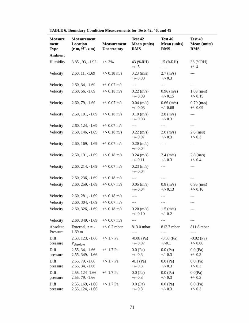
TABLE 6. Boundary Condition Measurements for Tests 42, 46, and 49
MeasurementType
MeasurementLocation (r m, θ°, z m)
Measurement Uncertainty
Test 42Mean (units)RMS
Test 46Mean (units)RMS
Test 49Mean (units)RMS
Ambient
Humidity 3.85 , 93, -1.92 +/- 3% 43 (%RH)+/- 5
15 (%RH)-----
38 (%RH)+/- 4
Velocity 2.60, 11, -1.69 +/- 0.18 m/s 0.23 (m/s)+/- 0.08
2.7 (m/s)+/- 0.3
---
Velocity 2.60, 34, -1.69 +/- 0.07 m/s --- --- ---
Velocity 2.60, 56, -1.69 +/- 0.18 m/s 0.22 (m/s)+/- 0.08
0.96 (m/s)+/- 0.15
1.03 (m/s)+/- 0.15
Velocity 2.60, 79, -1.69 +/- 0.07 m/s 0.04 (m/s)+/- 0.03
0.66 (m/s)+/- 0.08
0.70 (m/s)+/- 0.09
Velocity 2.60, 101, -1.69 +/- 0.18 m/s 0.19 (m/s)+/- 0.08
2.8 (m/s)+/- 0.3
---
Velocity 2.60, 124, -1.69 +/- 0.07 m/s --- --- ---
Velocity 2.60, 146, -1.69 +/- 0.18 m/s 0.22 (m/s)+/- 0.07
2.0 (m/s)+/- 0.3
2.6 (m/s)+/- 0.3
Velocity 2.60, 169, -1.69 +/- 0.07 m/s 0.20 (m/s)+/- 0.04
--- ---
Velocity 2.60, 191, -1.69 +/- 0.18 m/s 0.24 (m/s)+/- 0.11
2.4 (m/s)+/- 0.3
2.8 (m/s)+/- 0.4
Velocity 2.60, 214, -1.69 +/- 0.07 m/s 0.23 (m/s)+/- 0.04
--- ---
Velocity 2.60, 236, -1.69 +/- 0.18 m/s --- --- ---
Velocity 2.60, 259, -1.69 +/- 0.07 m/s 0.05 (m/s)+/- 0.04
0.8 (m/s)+/- 0.13
0.95 (m/s)+/- 0.16
Velocity 2.60, 281, -1.69 +/- 0.18 m/s ---- --- ---
Velocity 2.60, 304, -1.69 +/- 0.07 m/s --- --- ---
Velocity 2.60, 326, -1.69 +/- 0.18 m/s 0.20 (m/s)+/- 0.10
1.5 (m/s)+/- 0.2
---
Velocity 2.60, 349, -1.69 +/- 0.07 m/s --- --- ---
Absolute Pressure
External, z = -1.69 m
+/- 0.2 mbar 813.0 mbar----
812.7 mbar----
811.8 mbar----
Diff. pressure
2.63, 123, -1.66Pabsolute
+/- 1.7 Pa -0.08 (Pa)+/- 0.07
-0.03 (Pa)+/-0.1
-0.02 (Pa)+/- 0.06
Diff. pressure
2.55, 34, -1.662.55, 349, -1.66
+/- 1.7 Pa 0.0 (Pa)+/- 0.3
0.0 (Pa)+/- 0.3
0.0 (Pa)+/- 0.3
Diff. pressure
2.55, 79, -1.662.55, 34, -1.66
+/- 1.7 Pa -0.1 (Pa)+/- 0.3
0.0 (Pa)+/- 0.3
0.0 (Pa)+/- 0.3
Diff. pressure
2.55, 124 -1.662.55, 79, -1.66
+/- 1.7 Pa 0.0 (Pa)+/- 0.3
0.0 (Pa)+/- 0.3
0.0(Pa)+/- 0.3
Diff. pressure
2.55, 169, -1.662.55, 124, -1.66
+/- 1.7 Pa 0.0 (Pa)+/- 0.3
0.0 (Pa)+/- 0.3
0.0 (Pa)+/- 0.3
71

Diff. pressure
2.55, 214, -1.662.55, 169, -1.66
+/- 1.7 Pa -0.1 (Pa)+/- 0.3
0.0 (Pa)+/- 0.3
0.0 (Pa)+/- 0.3
Diff. pressure
2.55, 259, -1.662.55, 214, -1.66
+/- 1.7 Pa -0.0 (Pa)+/- 0.3
0.0 (Pa)+/- 0.3
0.0 (Pa)+/- 0.3
Diff. pressure
2.55, 304, -1.662.55, 259, -1.66
+/- 1.7 Pa (0.0 Pa)+/- 0.3
0.0 (Pa)+/- 0.3
0.0 (Pa)+/- 0.3
Diff. pressure
2.55, 349, -1.662.55, 304, -1.66
+/- 1.7 Pa 0.0 (Pa)+/- 0.3
0.0 (Pa)+/- 0.3
0.0 (Pa)+/- 0.3
Tempera-ture
3.85, 93°, -1.92 +/- 10°K 20 (°C)-----
26 (°C)-----
----
Plume
Diluent flow rate
In high pres-sure manifold
+/- 0.001 (kg/s)
0.030 (kg/s)+/- 0.001
N/A N/A
Diluent line tem-perature
In high pres-sure manifold
+/- 10 °K 2 (°C)-----
N/A N/A
Diluent line pres-sure
In high pres-sure manifold
+/- 7 kPa 1.14 (MPa)-----
N/A N/A
Fuel flow rate
In high pres-sure manifold
+/- 0.001 (kg/s)
N/A 0.0175(kg/s)+/- 0.0005
0.0436 (kg/s)+/-0.0004
Fuel line tempera-ture
In high pres-sure manifold
+/- 10 °K N/A 16 (°C)-----
-16 (°C)-----
Fuel line pressure
In high pres-sure manifold
+/- 7kPa N/A 1.19 (MPa)+/- 0.01
1.31 (MPa)+/- 0.01
Diff pressure
0.47, 193, 0.0Pabsolute
+/- 1.7 Pa 0.0 (Pa)+/- 0.07
-0.1 (Pa)+/- 0.1
-0.1 (Pa)+/- 0.1
Diff pressure
0.47, 193, 0.00.47, 193, 0.97
+/- 1.7 Pa ---- 9.8 (Pa)+/- 0.3
9.7 (Pa)+/- 0.3
Tempera-ture - Dif-fuser
0.0, 90, -0.05 +/- 10°K 18 (°C)-----
20 (°C)-----
29 (°C)-----
Outflow
Dyn. pressure
0.00, 90, 4.56 +/- 2.0 (kg/s2/m)
5.4 (kg/s2/m)+/- 1.0
19. (kg/s2/m)+/- 3.
18. (kg/s2/m)+/- 3.
Dyn. pressure
0.27, 90, 4.56 +/- 2.0 (kg/s2/m)
1.5 (kg/s2/m)+/- 0.8
11. (kg/s2/m)+/- 3.
11. (kg/s2/m)+/- 3.
Dyn. pressure
0.53, 90, 4.56 +/- 2.0 (kg/s2/m)
-0.1 (kg/s2/m)+/- 0.04
0.5 (kg/s2/m)+/- 1.0
1.9 (kg/s2/m)+/- 1.7
Dyn. pressure
0.80, 90, 4.56 +/- 2.0 (kg/s2/m)
-0.1 (kg/s2/m)+/- 0.04
0.2 (kg/s2/m)+/- 0.8
0.3 (kg/s2/m)+/- 0.9
TABLE 6. Boundary Condition Measurements for Tests 42, 46, and 49
MeasurementType
MeasurementLocation (r m, θ°, z m)
Measurement Uncertainty
Test 42Mean (units)RMS
Test 46Mean (units)RMS
Test 49Mean (units)RMS
72
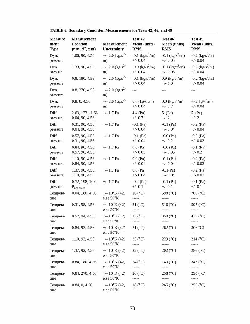
Dyn. pressure
1.06, 90, 4.56 +/- 2.0 (kg/s2/m)
-0.1 (kg/s2/m)+/- 0.04
-0.1 (kg/s2/m)+/- 0.05
-0.2 (kg/s2/m)+/- 0.04
Dyn. pressure
1.33, 90, 4.56 +/- 2.0 (kg/s2/m)
-0.0 (kg/s2/m)+/- 0.04
-0.1 (kg/s2/m)+/- 0.05
-0.2 (kg/s2/m)+/- 0.04
Dyn. pressure
0.8, 180, 4.56 +/- 2.0 (kg/s2/m)
-0.1 (kg/s2/m)+/- 0.04
0.9 (kg/s2/m)+/- 1.0
-0.2 (kg/s2/m)+/- 0.04
Dyn. pressure
0.8, 270, 4.56 +/- 2.0 (kg/s2/m)
--- --- ---
Dyn. pressure
0.8, 0, 4.56 +/- 2.0 (kg/s2/m)
0.0 (kg/s2/m)+/- 0.04
0.0 (kg/s2/m)+/- 0.7
-0.2 kg/s2/m)+/- 0.04
Diff. pressure
2.63, 123, -1.660.04, 90, 4.56
+/- 1.7 Pa 4.4 (Pa)+/- 0.7
5. (Pa)+/- 2.
5. (Pa)+/- 2.
Diff pressure
0.31, 90, 4.560.04, 90, 4.56
+/- 1.7 Pa -0.1 (Pa)+/- 0.04
-0.1 (Pa)+/- 0.04
-0.2 (Pa)+/- 0.04
Diff pressure
0.57, 90, 4.560.31, 90, 4.56
+/- 1.7 Pa -0.1 (Pa)+/- 0.04
-0.0 (Pa)+/- 0.2
-0.2 (Pa)+/- 0.03
Diffpressure
0.84, 90, 4.560.57, 90, 4.56
+/- 1.7 Pa 0.0 (Pa)+/- 0.03
-0.0 (Pa)+/- 0.05
-0.1 (Pa)+/- 0.2
Diff pressure
1.10, 90, 4.560.84, 90, 4.56
+/- 1.7 Pa 0.0 (Pa)+/- 0.04
-0.1 (Pa)+/- 0.04
-0.2 (Pa)+/- 0.03
Diff pressure
1.37, 90, 4.561.10, 90, 4.56
+/- 1.7 Pa 0.0 (Pa)+/- 0.04
-0.1(Pa)+/- 0.04
-0.2 (Pa)+/- 0.03
Diff pressure
0.72, 198, 10.0Pabsolute
+/- 1.7 Pa -0.2 (Pa)+/- 0.1
-0.1 (Pa)+/- 0.1
-0.1 (Pa)+/- 0.1
Tempera-ture
0.04, 180, 4.56 +/- 10°K (42)else 50°K
16 (°C)-----
598 (°C)-----
706 (°C)-----
Tempera-ture
0.31, 98, 4.56 +/- 10°K (42) else 50°K
31 (°C)-----
516 (°C)-----
597 (°C)-----
Tempera-ture
0.57, 94, 4.56 +/- 10°K (42) else 50°K
23 (°C)-----
350 (°C)-----
435 (°C)-----
Tempera-ture
0.84, 93, 4.56 +/- 10°K (42) else 50°K
21 (°C)-----
262 (°C)-----
306 °C)-----
Tempera-ture
1.10, 92, 4.56 +/- 10°K (42) else 50°K
33 (°C)-----
229 (°C)-----
214 (°C)-----
Tempera-ture
1.37, 92, 4.56 +/- 10°K (42) else 50°K
22 (°C)-----
202 (°C)-----
286 (°C)-----
Tempera-ture
0.84, 180, 4.56 +/- 10°K (42) else 50°K
24 (°C)-----
143 (°C)-----
347 (°C)-----
Tempera-ture
0.84, 270, 4.56 +/- 10°K (42) else 50°K
20 (°C)-----
258 (°C)-----
290 (°C)-----
Tempera-ture
0.84, 0, 4.56 +/- 10°K (42) else 50°K
18 (°C)-----
265 (°C)-----
255 (°C)-----
TABLE 6. Boundary Condition Measurements for Tests 42, 46, and 49
MeasurementType
MeasurementLocation (r m, θ°, z m)
Measurement Uncertainty
Test 42Mean (units)RMS
Test 46Mean (units)RMS
Test 49Mean (units)RMS
73

PIV/PLIF Results
Three tests were chosen for data analysis, consisting of one helium test (Test #42), one hydrogen test (Test #46), and one methane test (Test #49). These represent the best test results for each type of plume fluid. The plume inlet parameters for each test were listed earlier in Table 5.
Solid Surface
Tempera-ture - Ground
0.53, 135, 0.0 +/- 10°K (42) else 50°K
21 (°C)-----
133 (°C)-----
66 (°C)-----
Tempera-ture - Ground
0.74, 135, 0.0 +/- 10°K (42)else 50°K
28 (°C)-----
104 (°C)-----
98 (°C)-----
Tempera-ture - Ground
0.97, 135, 0.0 +/- 10°K (42)else 50°K
---- 68 (°C)-----
55 (°C)-----
Tempera-ture - Cyl. Shield
2.91, 141, -1.49 +/- 10°K (42)else 50°K
21 (°C)-----
---- 34 (°C)-----
Tempera-ture - Cyl. Shield
2.91, 141, -0.32 +/- 10°K (42)else 50°K
---- 38 (°C)-----
33 (°C)-----
Tempera-ture - Cyl. Shield
2.91, 141, 0.84 +/- 10°K (42) else 50°K
28 (°C)-----
67 (°C)-----
64 (°C)-----
Tempera-ture - Wall
3.05, 132, 1.64 +/- 10°K (42)else 50°K
23 (°C)-----
38 (°C)-----
47 (°C)-----
Tempera-ture - Vert. Shield
2.95, 132, 3.01 +/- 10°K (42) else 50°K
---- 73 (°C)-----
67 (°C)-----
Tempera-ture - Slant Shield
2.29, 132, 3.91 +/- 10°K (42)else 50°K
23 (°C)-----
85 (°C)-----
80 (°C)-----
Tempera-ture -Slant Shield
1.81, 132, 4.28 +/- 10°K (42) else 50°K
-- (°C)-----
146 (°C)-----
102 (°C)-----
TABLE 6. Boundary Condition Measurements for Tests 42, 46, and 49
MeasurementType
MeasurementLocation (r m, θ°, z m)
Measurement Uncertainty
Test 42Mean (units)RMS
Test 46Mean (units)RMS
Test 49Mean (units)RMS
74

ined ent
base
egen ntum inlet a rge y the it gins ts.
ong ), then
of the to the f the
arge This arly
ation ith the rtical . The cture
ents ed by ycles.
, by y be e are .
PIV Results and Flow Visualization Observations
The three cases examined demonstrated the quasi-periodic instability commonly referred to as “puffing.” All three plumes had a nominal puffing frequency of 1.5 Hz, as determby timing puff events on video displays. This puffing frequency is in excellent agreemwith the Cetegen and Ahmed (1993) correlation, f=1.5D-0.5, providing additional verification of their assumption that the puffing frequency is determined by the plumediameter, independent of heat release rate.
The puffing behavior has been described in many previous investigations (e. g., Cetand Ahmed, 1993). These observations will be summarized here from a linear momeperspective. As light plume fluid exits the plume inlet, it slowly accumulates near the until it reaches sufficient volume to trigger the Rayleigh-Taylor instability caused by heavy fluid overlying a lighter fluid. The lighter plume fluid then bursts upward as a lavortex, approximately the size of the plume inlet. The small amount of vorticity shed bburner lip is of opposite sign to this large buoyant plume vortex. As the vortex rises,entrains air below it, drawing the plume fluid down to a thin “neck.” The neck then beto thicken, until another volume of buoyant fluid is accumulated and the cycle repea
From a vortex dynamics perspective (Tieszen, et al., 1996), vorticity is generated continuously along the plume air interface due to baroclinic vorticity generation. As las the density gradient is not aligned with the pressure gradient (i.e., stably stratifiedthe flow will be “unstable”. The vorticity produced along the plume air interface amalgamates into larger and larger structures as the vorticity is advected downstreamtoe of the plume. However, in plumes (as opposed to jets) the advection rate relativeamalgamation rate is not large (as evidenced by the termination of the central core oplume in less than one diameter versus several diameters for a jet). Therefore, the lvortical structures that form induce a significant radial inflow at the base of the plume.inflow has sufficient momentum to redirect the flow near the toe of the plume from nevertical to nearly horizontal. The change in angle affects the baroclinic vorticity generrate at the base of the plume because the density gradient is more closely aligned wvertical pressure gradient. As the large coherent vortex is advected downstream, itsinfluence on the radial inflow at the base of the plume diminishes. As a result, the vemomentum of the plume begins to tip the plume-air interface back toward the verticalmisalignment then generates vorticity which amalgamates into a large coherent struand the process repeats itself.
For all three cases examined here, the puffing is quasi-periodic, with most puffing evoccurring at or near the average puffing frequency (1.5 Hz in this case), but with theoccasional occurrence of an aperiodic puff. The average puff frequency was determinanalysis of video images of the overall plume, based on passage of at least 50 puff cThe cycles selected for Figure 12 through Figure 33 were similarly selected visuallyinspection of scanned images to determine when the pattern repeated. This can onlexpected to be accurate to within about 50 ms. Pressure traces on the burner surfacprobably a more reliable indicator of the puff frequency (Cetegen and Ahmed, 1993)
75

The PIV-measured velocity fields for the three cases of interest are shown in Figure 12 through Figure 36. While the overall velocity fields are similar in the three cases, i.e., all show similar puffing behavior, there are quantitative differences related to the different test conditions (see Table 5), as will be detailed below.
Helium Plume. Figure 12 through Figure 17 show selected images and velocity fields from one puff cycle of a helium plume test. The nominal puffing period is 667 msec per puff. The camera frame rate was 180 frames/s, so an image was recorded every 5.6 ms. Only every 24th frame is shown in this sequence. The puff cycle selected here had a period very close to the 1.5 Hz average. The plume centerline velocity increases from a few centimeters per second near the inlet to as high as 5.3 m/s at a vertical location 900 mm above the burner (Figure 17).
Puffing is less strong for helium than for the reacting gases, possibly because the helium plume buoyancy is decreased by mixing with the surrounding air, while for the reacting gases buoyant fluid is continuously generated. The large toroidal vortices reach a maximum diameter of about 1.0 m, equal to the plume inlet diameter.
PIV in the non-reacting helium plume has several advantages over the reacting cases. First, there is no volumetric expansion due to high temperatures, so the seeding density can be pretty well fixed. Also, the seed particles are not destroyed as they are in the reacting cases.
Figure 12. PIV frame at 0 msec from start of one cycle of a helium plume puff period.
76

Figure 13. PIV frame 133 msec from start of one cycle of a helium plume puff period.
Figure 14. PIV frame 267 msec from start of one cycle of a helium plume puff period.
77

Figure 15. PIV frame 400 msec from start of one cycle of a helium plume puff period.
Figure 16. PIV frame 533 msec from start of one cycle of a helium plume puff period.
78

The effect of the vortex on the velocity field can be seen from the centerline profiles of the axial velocity component presented in Figure 18 for the helium plume. The three lines shown correspond to the three times in the puffing cycle. The solid line, at time t=226 msec, shows a gradual acceleration of the fluid along the centerline from the inlet velocity of 0.29 m/s for this case to a maximum downstream value of 2.8 m/s. At this time, no well-developed vortex is present in the flow. At t=447 msec, a large, well-formed vortex is located at an elevation of 300 mm. A rapid increase in the centerline velocity to about 3 m/s is seen at 180 mm. This distance corresponds to the upstream edge of the vortex where the flow has begun to neck down due to the rotational motion of the vortex, resulting in a rapid acceleration of the central fluid. Finally, at t= 667 msec (dotted line), the vortex is located at about 500 mm downstream and again a rapid rise in the axial velocity occurs near the upstream edge of the vortex to a maximum value of nearly 5 m/s.
Instantaneous radial profiles of the axial and radial velocity component in the helium plume are shown in Figure 19 and Figure 20, respectively. In each figure, profiles are shown at four distances above the burner inlet. Here the flow centerline is located at a radial distance of 640 mm. Figure 19 a) and Figure 20 a) show profiles near the start of the puffing cycle when the formation of vortical structures associated with puffing has just begun, while Figure 19 b) and Figure 20 b) show the profiles at a time of maximum centerline acceleration. In the sign convention adopted here, positive axial velocity corresponds to flow in the downstream direction, while positive and negative radial velocity corresponds to flow in the right and left directions, respectively. (Note that in this convention positive
Figure 17. PIV frame 667 msec from start of one cycle of a helium plume puff period.
79
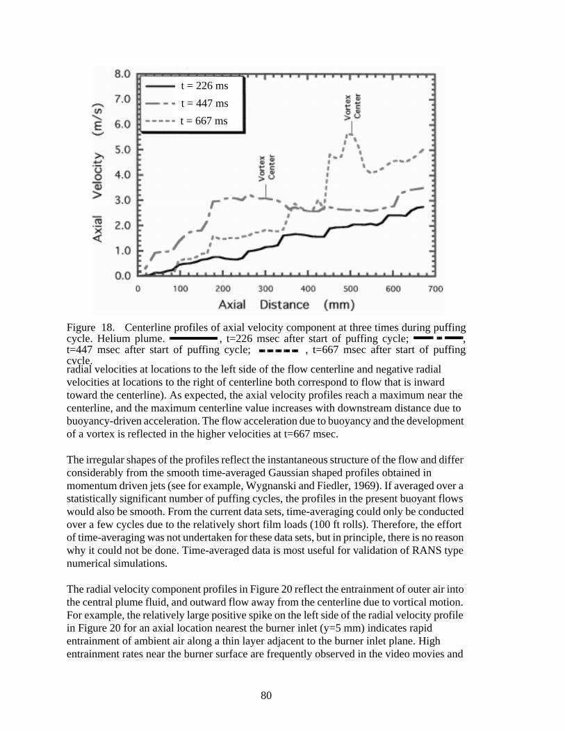
radial velocities at locations to the left side of the flow centerline and negative radial velocities at locations to the right of centerline both correspond to flow that is inward toward the centerline). As expected, the axial velocity profiles reach a maximum near the centerline, and the maximum centerline value increases with downstream distance due to buoyancy-driven acceleration. The flow acceleration due to buoyancy and the development of a vortex is reflected in the higher velocities at t=667 msec.
The irregular shapes of the profiles reflect the instantaneous structure of the flow and differ considerably from the smooth time-averaged Gaussian shaped profiles obtained in momentum driven jets (see for example, Wygnanski and Fiedler, 1969). If averaged over a statistically significant number of puffing cycles, the profiles in the present buoyant flows would also be smooth. From the current data sets, time-averaging could only be conducted over a few cycles due to the relatively short film loads (100 ft rolls). Therefore, the effort of time-averaging was not undertaken for these data sets, but in principle, there is no reason why it could not be done. Time-averaged data is most useful for validation of RANS type numerical simulations.
The radial velocity component profiles in Figure 20 reflect the entrainment of outer air into the central plume fluid, and outward flow away from the centerline due to vortical motion. For example, the relatively large positive spike on the left side of the radial velocity profile in Figure 20 for an axial location nearest the burner inlet (y=5 mm) indicates rapid entrainment of ambient air along a thin layer adjacent to the burner inlet plane. High entrainment rates near the burner surface are frequently observed in the video movies and
Figure 18. Centerline profiles of axial velocity component at three times during puffingcycle. Helium plume. , t=226 msec after start of puffing cycle; ,t=447 msec after start of puffing cycle; , t=667 msec after start of puffingcycle.
t = 226 ms
t = 447 ms
t = 667 ms
80

Figure 19. Radial profiles of axial velocity component in helium plume. a) t=226 msecafter start of puffing cycle; b) t=667 msec after start of puffing cycle. Plume centerline at aradial distance of 640 mm in this figure.
81

Figure 20. Radial profiles of radial velocity component in helium plume. a) t=226 msecafter start of puffing cycle; b) t=667 msec after start of puffing cycle. Plume centerline at aradial distance of 640 mm in this figure.
82

iod.
are due to the rotational motion of newly formed vortices located just downstream of the burner surface, which induces significant radial inflow near the base of the plume. Generally, the radial velocity profiles reflect entrainment of ambient air into the plume fluid (positive and negative velocities on the left and right sides of the centerline, respectively). However, when a vortex is present these signs reverse and outward flow of the plume fluid due to vortical rotation becomes significant. For example, the negative and positive radial velocity peaks seen on the left and right sides of the centerline in the y=5 mm profile of Figure 20 b) correspond to the presence of large rotating vortex seen in Figure 17.
Simultaneous planar laser-induced fluorescence (PLIF) of acetone vapor seeding the helium plume was attempted, with acetone concentrations as high as 2%. The same laser light sheet used for PIV was used to excite the acetone, and the visible fluorescent signal was recorded on a second camera. However, in all tests to date, the acetone fluorescence signal is too weak to provide the desired concentration field map.
Methane Fire. Figure 21 through Figure 26 show selected images and velocity fields from one puff cycle of a methane fire. The nominal puffing period is 667 msec per puff. The camera frame rate was 185 frames/s, so an image was recorded every 5.4 msec. Only every 24th frame is shown in this sequence. The period of the selected cycle was approximately 649 msec, for a frequency of 1.54 Hz. While difficult to see in the figures because of the overlying velocity vectors, the films clearly show a fluorescence signal which we associate with polycyclic-aromatic hydrocarbons (PAH’s). The PAH fluorescence gives a goodindicator of the reaction zone at the fuel-air interface.
Figure 21. PIV frame 0 msec from start of one cycle of a methane plume puff per
83
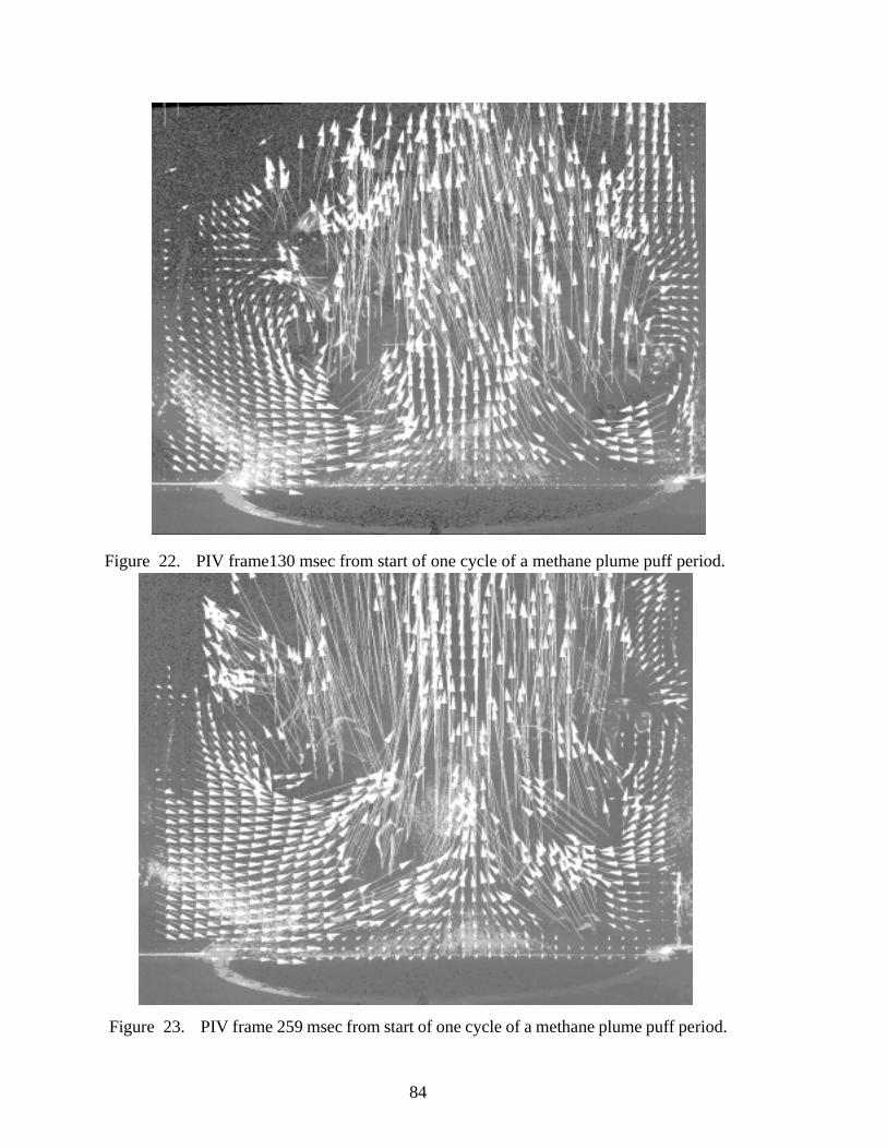
Figure 22. PIV frame130 msec from start of one cycle of a methane plume puff period.
Figure 23. PIV frame 259 msec from start of one cycle of a methane plume puff period.
84
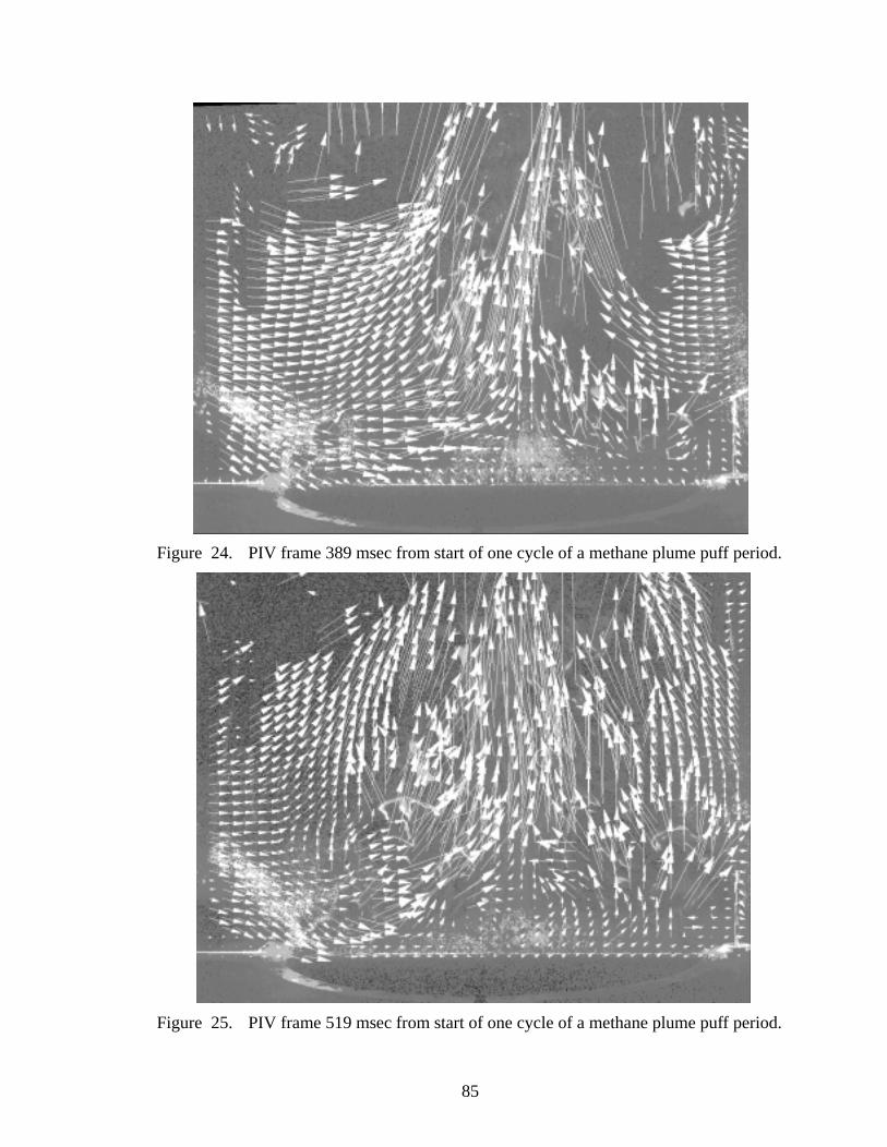
Figure 24. PIV frame 389 msec from start of one cycle of a methane plume puff period.
Figure 25. PIV frame 519 msec from start of one cycle of a methane plume puff period.
85

There are usually 1 or 2 large vortices present in the FLAME facility before the fire exits the chimney. The methane fire is very bright, because of soot formation, and gets much brighter when the seed particles begin to flow in. However, as can be seen from the methane figures, PIV can be performed on the remaining seed particles. The presence of soot does not seem to harm the PIV image significantly. The PAH signal is a bigger concern, since the cross-correlation was seen to track the movement of these reacting, rapidly evolving structures rather than the seed particles nearby. Such vectors were removed from the methane figures by application of a nearest-neighbor validation scheme.
The centerline profiles for the CH4 flame shown in Figure 27 shows a similar acceleration with increasing elevation as in the helium plume. In the CH4 flame, again the presence of a vortex results in noticeable fluid acceleration along the centerline at a downstream distance of 180 mm (time=0 msec) and at 400mm (t=222 msec). Rapid velocity increases in the profiles for t=0 msec at 500 mm and for t=444 msec at 400 mm are also observed, although no vortex is present in the images near these locations. It is likely that these are simply random velocity fluctuations and a further indication of the complexity of these flows. The large toroidal vortices reach a maximum diameter of about 1.1 m, just larger than the plume inlet. The maximum centerline velocities reach 5.22 m/s at a vertical location 900 mm above the burner (Figure 24), a fifty times acceleration.
Hydrogen Fire. Figure 28 through Figure 33 show selected images and velocity from one puff cycle of a hydrogen fire test. The nominal puffing period is 667 msec per puff. The
Figure 26. PIV frame 649 msec from start of one cycle of a methane plume puff period.
86
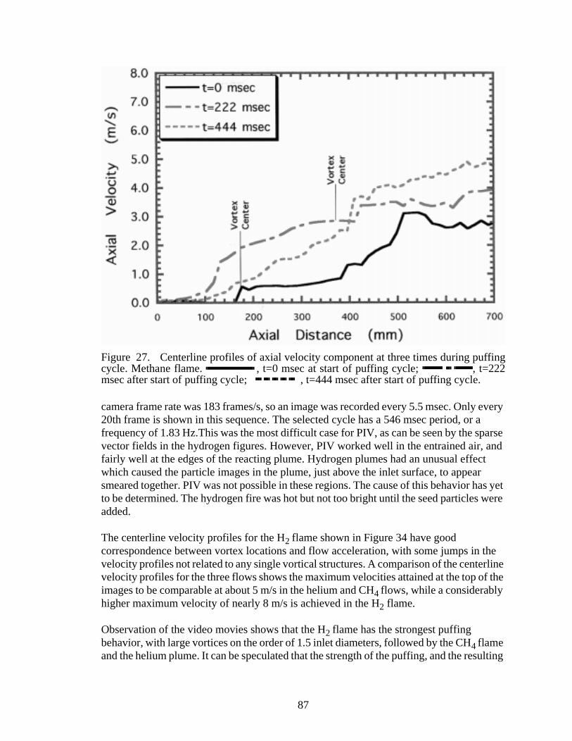
camera frame rate was 183 frames/s, so an image was recorded every 5.5 msec. Only every 20th frame is shown in this sequence. The selected cycle has a 546 msec period, or a frequency of 1.83 Hz.This was the most difficult case for PIV, as can be seen by the sparse vector fields in the hydrogen figures. However, PIV worked well in the entrained air, and fairly well at the edges of the reacting plume. Hydrogen plumes had an unusual effect which caused the particle images in the plume, just above the inlet surface, to appear smeared together. PIV was not possible in these regions. The cause of this behavior has yet to be determined. The hydrogen fire was hot but not too bright until the seed particles were added.
The centerline velocity profiles for the H2 flame shown in Figure 34 have good correspondence between vortex locations and flow acceleration, with some jumps in the velocity profiles not related to any single vortical structures. A comparison of the centerline velocity profiles for the three flows shows the maximum velocities attained at the top of the images to be comparable at about 5 m/s in the helium and CH4 flows, while a considerably higher maximum velocity of nearly 8 m/s is achieved in the H2 flame.
Observation of the video movies shows that the H2 flame has the strongest puffing behavior, with large vortices on the order of 1.5 inlet diameters, followed by the CH4 flame and the helium plume. It can be speculated that the strength of the puffing, and the resulting
Figure 27. Centerline profiles of axial velocity component at three times during puffingcycle. Methane flame. , t=0 msec at start of puffing cycle; , t=222msec after start of puffing cycle; , t=444 msec after start of puffing cycle.
87
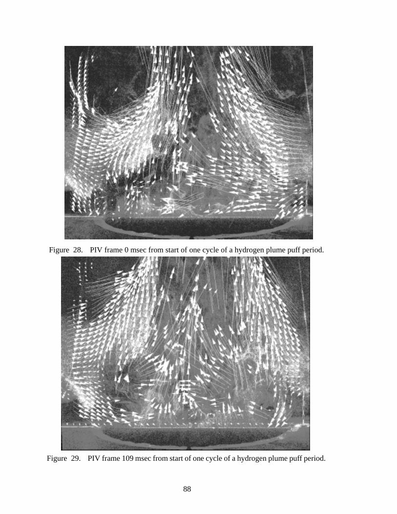
Figure 28. PIV frame 0 msec from start of one cycle of a hydrogen plume puff period.
Figure 29. PIV frame 109 msec from start of one cycle of a hydrogen plume puff period.
88

Figure 30. PIV frame 218 msec from start of one cycle of a hydrogen plume puff period.
Figure 31. PIV frame 328 msec from start of one cycle of a hydrogen plume puff period.
89
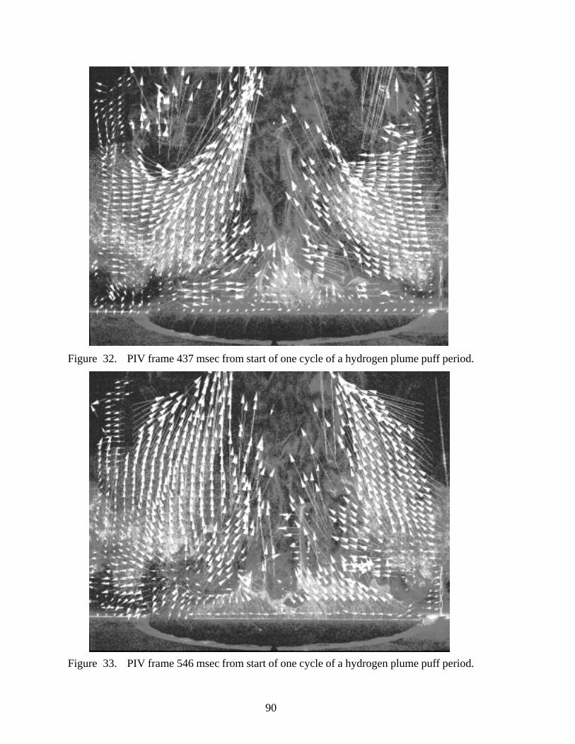
Figure 32. PIV frame 437 msec from start of one cycle of a hydrogen plume puff period.
Figure 33. PIV frame 546 msec from start of one cycle of a hydrogen plume puff period.
90

acceleration of gases along the centerline, is directly related to buoyancy forces generated by the density difference between the plume fluid and the surrounding air. One measure of the buoyancy forces is the Richardson number, Ri = (ρair / ρplume - 1)gD/V2 which is the ratio of buoyancy force to inertia forces. The cold inlet Ri for the current flows is 680 (CH4 flame), 730 (helium plume) and 1100 (H2 flame). Even without considering reaction heat release, the test conditions for the H2 flame clearly correspond to the strongest buoyancy forces, consistent with the observations. Further, buoyancy in the helium decreases due to mixing with high density entrained air, while in the reacting flames, combustion heat release continually regenerates buoyant, high-temperature combustion gases. Thus, the CH4 flame exhibits stronger puffing than the helium plume even though the cold inlet Ri is essentially the same.
The radial profiles of axial and radial velocity components in the H2 flame shown in Figure 35 and Figure 36, respectively, exhibit similar behavior to the helium plume. In the axial velocity component profiles, the maximum velocity again occurs near the flow centerline and increases with downstream distance. As noted previously, the maximum velocities achieved in the H2 flame, nearly 8 m/s, are 40 percent higher than in the helium plume or the CH4 flame due to increased buoyancy-driven acceleration of the low density flame
Figure 34. .Centerline profiles of axial velocity component at three times during puffingcycle. Hydrogen flame. , t=187 msec after start of puffing cycle; ,t=364 msec after start of puffing cycle; , t=546 msec after start of puffingcycle.
t = 187 ms
t = 364 ms
t = 546 ms
91
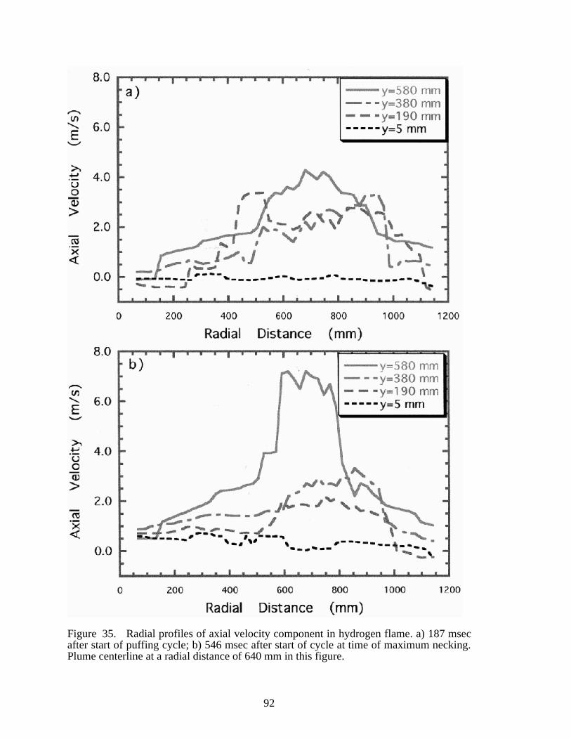
Figure 35. Radial profiles of axial velocity component in hydrogen flame. a) 187 msecafter start of puffing cycle; b) 546 msec after start of cycle at time of maximum necking.Plume centerline at a radial distance of 640 mm in this figure.
92

Figure 36. Radial profiles of radial velocity component in hydrogen flame. a) 187 msecafter start of puffing cycle; b) 546 msec after start of cycle at time of maximum necking.Plume centerline at a radial distance of 640 mm in this figure.
93

gases. Consistent with the stronger puffing and vorticity generated in the H2 flame, stronger entrainment of ambient air is also observed. This increase can be seen from the radial component profiles in Figure 36. At 187 msec after the start of the puffing cycle, the maximum entrainment velocities are about 1 m/s, which is comparable with entrainment velocities in the helium plume seen in Figure 20. At the downstream location of y=580 mm, the maximum radial velocity is nearly 2 m/s inward toward the centerline. This high entrainment rate is due to the combined effects of entrainment by the high velocity, necked region of the flow upstream of the vortex, and the rotational motion of the vortex which is located near the upper edge of the image and results in additional inward convection due to its rotational motion.
94

ConclusionsFour goals were defined for this Laboratory Directed Research and Development (LDRD) study. Each goal and progress toward that goal are given below.
The first goal of this LDRD is to demonstrate that velocity fields are measurable with two orders of magnitude resolution in two spatial dimensions and time. This goal has been completely met. The developed PIV system in the FLAME facility can meet these resolution requirements for completely non-reacting plume flows. For reacting-flows, the flow field velocities external to the reacting plume can be measured and for methane flows, the non-reacting plume core can also be measured. However, with the glass seed particles chosen for this study, the hot product region was not measurable due to the burn-up of the particles. Smaller metal oxide particles could be used in this region without burning up. However, they may not be resolvable at the 1 m by 1 m nominal scale desired for the flow fields. The performance of the metal oxide particles was not tried due to a lack of time.
The second goal of this LDRD is to apply the PIV technology to study the physics of fully turbulent, buoyant, non-reacting and reacting flows. This goal has been completely met. A canonical, plume flow was developed with a 1 meter base diameter. Flow characteristics were measured for non-reacting helium, and reacting hydrogen and methane flows. Further, two tests were run with mixtures of helium and nitrogen demonstrating a capability to do two-fluid plume sources. The near source region of non-reacting and reacting plumes (fires) is an important flow for Sandia National Laboratories and has received little prior attention in the literature. It is the region in which baroclinic vorticity generation is the strongest while advected vorticity is the weakest. The data generated provide important insight into the dynamics of buoyant turbulence and its respective time and length scales.
The third goal of this LDRD is to demonstrate that data sets of sufficient quality to support validation of numerical simulation tools can be obtained for buoyant, non-reacting and reacting flows. This goal has been met with partial success. These tests have demonstrated that data sets of sufficient quality can be generated, but fell short in actually generating the data sets. The principal reason that the data sets analyzed are not of sufficient quality to be considered validation data is the failure of the boundary condition measurements. The failures were principally due to three reasons, the velocity gauges selected were not sufficiently rugged to survive the environment, the differential pressure gauges in some cases did not have sufficient sensitivity, and there was sufficient electronic noise during the tests to create offsets. While these reasons prevented the current tests from being of validation quality, they do not prevent the data from being used scientifically. Further, with sufficient care, these problems can be eliminated. A measure of the confidence that these problems can be eliminated is that follow-on funding has been obtained from a defense programs validation program to obtain validation data for a new numerical simulation tool under development for fires.
95
s are a that hey are btain al
The fourth goal of the LDRD is to obtain simultaneous scalar field measurements with velocity field measurements. This goal has been met with partial success. We were not able to obtain acetone fluorescence with sufficient intensity to obtain a quantitative measure of the scalar field in the non-reacting helium flows. It is felt that through the use of an image intensifier, the weak images that were obtained could be amplified to the point of usability. An image intensifier system was assembled, but was not used in the testing due to time constraints. It is intended to try it in the follow-on tests. An alternative is to use a moderate density of small smoke particles as a means of distinguishing the plume from the ambient. The scattered light may interfere with the PIV measurement, however. We will examine this approach in the follow-on series if the acetone fluorescence proves intractable.
While the acetone fluorescence failed in the non-reacting helium fields, unexpected fluorescence signatures were gained in the reacting-flows. Of particular value is the signature in the reacting methane flows thought to be due to PAH’s. These signaturemarker for the flame interfaces. This information is quite insightful and clearly showsthe products tend to the elevated side of the flame zone as would be expected since thot and buoyant. The flame position as a function of time can be time averaged to othe mean location of the flame interface which will be useful in validation of numericsimulations.
96
ics,”
mes
s- VA,
y of
or of
ula-
ng in
1980,
in the
eatbus-
The
ReferencesAllen, M. G., Howe, R. D. and Hanson, R. K., 1986, Opt. Lett. 11, 126.
Adrian, R. J., 1991, “Particle Imaging Techniques for Experimental Fluid MechanAnnual Review of Fluid Mechanics, 23, Annual Reviews, Inc., Palo Alto, CA.
Baum, H. R., McGrattan, K. B., and Rehm, R. G., 1994, “Simulation of Smoke Plufrom Large Pool Fires,” The Twenty-Fifth Symposium (International) on Combus-tion, The Combustion Institute, pp. 1463-1469.
Blinov, V.I., and Khudyakov, G. N. 1961, “Diffusion Burning of Liquids,” English Tranlation: U.S. Army Engineering Research and Development Labs, Fort Belvoir,Report AERDL-T-1490-A.
Cattolica, R. J. and Vosen, S. R., 1986, Combustion Science & Technology, 48, 77.
Cetegen, B. M. and Ahmed, T. A., 1993, “Experiments on the Periodic InstabilitBuoyant Plumes and Pool Fires,” Combustion and Flame, 93:157-184.
Cetegen, B. M. and Kasper, K. D., 1996, “Experiments on the Oscillatory BehaviBuoyant Plumes Of Helium and Helium-Air Mixtures,” Physics of Fluids, 8:2974-2984.
Clemens, N. T. and Paul, P. H. 1995, Combustion and Flame 102:271-284.
Crauford, N. L., Liew, S. K., and Moss, J. B., 1985, “Experimental and Numerical Simtion of a Buoyant Fire,” Combustion and Flame, 61:63-77.
Dahm, W. J. A. and Dimotakis, P. E., 1987, “Measurements of Entrainment and MixiTurbulent Jets,” AIAA Journal, 25:1216-1223.
Friedlander, S. K., 1977, Smoke, Dust, and Haze, John Wiley and Sons, pp. 96, 164.
Fujiwara, K., Omenetto, N., Bradshaw, J. B., Bower, J. N. and Winefordner, J. D., Applied Spectroscopy, 34:85-94.
Gharib, M., 1996, “Perspective: The Experimentalist and the Problem of Turbulence Age of Supercomputers,” Journal of Fluids Engineering, 118:233-242.
Gritzo, L. A., Nicolette, V. F., Tieszen, S. R., Moya, J. L., and Holen, J., 1995, “HTransfer to the Fuel Surface in Large Pool Fires,” Transport Phenomena in Comtion, S. H. Chan, ed., Taylor and Francis, Washington, D. C.
Hamins, A., Yang, J. C., and Kashiwagi, T., 1992, “An Experimental Investigation OfPulsation Frequency of Flames,” The Twenty-Fourth Symposium (International) onCombustion, The Combustion Institute, pp. 1695-1702.
Haumann, J., Seitzman, J. M. and Hanson, R. K., 1986, Opt. Lett., 11, 776.
97

n of
Part
naly of
s and
obe
arch Pool
Dissi-
lent
theM,
yant
ersi-
ities,”
NY,
Handbook of Aviation Fuel Properties, 1983, Coordinating Research Council, AtlantaGeorgia, CRC No. 530, p. 71.
Holen, J., Brostrom, M., and Magnussen, B. F., 1990, “Finite Difference CalculatioPool Fires,” The Twenty-Third Symposium (International) on Combustion, TheCombustion Institute, pp. 1677-1683.
Keane, R. D. and Adrian, R. J., 1990, “Optimization of Particle Image Velocimeters:I: Double Pulsed Systems,” Meas. Sci. Technol., 1, 1202-1215.
Kent, L. A., and Schneider, M. E., 1987, “The Design and Application of Bi-DirectioVelocity Probes for Measurements in Large Pool Fires,” Instrument SocietAmerica Transactions, 26:25-32.
Kychakoff, G., Knapp, K., Howe, R. D. and Hanson, R. K, 1984, AIAA Journal, 22, 153.
Launder, B. E. and Spaulding, D. B., 1974, Computer Methods in Applied MechanicEngineering, v3, p. 269.
Lozano, A. and Hanson, R. K, 1992, Experiments in Fluids, 13, 369.
McCaffrey, B. J. and Heskestad, G., 1976, “A Robust Bidirectional Low-Velocity Prfor Flame and Fire Application,” Combustion and Flame, 26:125-127.
Malalasekera, W. M. G., Versteeg, H. K., and Gilchrist, K., 1996, “A Review of Reseand an Experimental Study on the Pulsation of Buoyant Diffusion Flames andFires,” Fire and Materials, 20:261-271.
Magnussen, B. F., 1981, Particulate Carbon Formation During Combustion, Plenum Pub-lishing Corporation.
Magnussen, B. F., Hjertager, B. H., Olsen, J. G., and Bhaduri, D., 1979, “The Eddy pation Concept, The Seventeenth Symposium (International) on Combustion, TheCombustion Institute, pp. 1383-1398.
Miller, J. H., Mallard, W. G. and Smyth, K. C., 1982, Combustion and Flame, 47:205-216.
Mungal, M. G. and Frieler, C. E., 1988, “The Effects of Damkohler Number in a TurbuShear Layer,” Combustion and Flame, 71:23-34.
Schneider, M. E., Keltner, N. R., and Kent, L. A., 1989, “Thermal Measurements inNuclear Winter Fire Test,” Sandia National Laboratories, Albuquerque, NSAND88-2839.
Seitzman, J. M., Kychakoff, G. and Hanson, R. K., 1985, Opt. Lett. 10, 439.
Shabbir, A. and George, W. K., 1994, “Experiments on a Round Turbulent BuoPlume,” Journal of Fluid Mechanics, 275:1-32.
Shah, N. G., 1979, “The Computation of Radiation Heat Transfer”, Ph.D. thesis, Univty of London, Faculty of Engineering.
Smagorinsky, J., 1993, “Some Historical Remarks on the Use of Nonlinear ViscosLarge Eddy Simulation of Complex Engineering and Geophysical Flows (eds. Galp-erin and Orszag), Press Syndicate of the University of Cambridge, New York,pp. 1-36.
98

ion,”
ulent
cale
lence
jet,”
s,”
ire,”
Smyth, K. C., Miller, J. H., Dorfman, R. C., Mallard, W. G. and Santoro, R. J., 1985, Com-bustion and Flame, 62:157-181.
Tennekes, H. and Lumley, J. L., 1972, A First Course In Turbulence, MIT Press.
Tieszen, S. R., Nicolette, V. F., Gritzo, L. A., Holen, J. K., Murray, D., and Moya, J. L.,1996, “Vortical Structures in Pool Fires: Observation, Speculation, and SimulatSandia National Laboratories, Albuquerque, NM, SAND96-2607.
Tieszen, S. R., Stamps, D. W., and O’Hern, T. J., 1996, “A Heuristic Model of TurbMixing Applied to Blowout of Turbulent Jet Diffusion Flames,” Combustion andFlame 106:442-466.
Weckman, E. J. and Sobiesiak, A., 1988, “The Oscillatory Behaviour of Medium-SPool Fires,” The Twenty-Second Symposium (International) on Combustion, TheCombustion Institute, pp. 1299-1310.
Weckman, E. J. and Strong, A. B., 1996, “Experimental Investigation of the TurbuStructure of Medium-Scale Methanol Pool Fires,” Combustion and Flame, 105:245-266.
Wygnanski, I. and Fiedler, H., 1969, “Some measurements in the self-preservingJournal of Fluid Mechanics, 38:577-593.
Willert, C., 1996, “The Fully Digital Evaluation of Photographic PIV RecordingApplied Scientific Research, 56, 79-102.
Zhou, X. C. and Gore, J. P., 1995, “Air Entrainment Flow Field Induced by a Pool FCombustion and Flame, 100:52-60.
99
DISTRIBUTION:
1 MS9051 L. A. Rahn, 83514 MS9051 R. W. Schefer, 83511 MS0841 P. J. Hommert, 91001 MS0828 T. C. Bickel, 91011 MS0826 W. L. Hermina, 91114 MS0826 T. J. O’Hern, 91111 MS0834 A. C. Ratzel, 91121 MS0834 T. W. Grasser, 91121 MS0836 C. W. Peterson, 9116
10 MS0836 S. R. Tieszen, 91161 MS0865 J. L. Moya, 97351 MS0865 R. W. Oliver, 97351 MS1135 J. R. Garcia, 97612 MS1135 L.D. Perea, 97611 MS1135 M. Martinez, 9761
1 MS0188 LDRD Office, 45231 MS9018 Central Technical Files, 8940-22 MS0899 Technical Library, 49162 MS0619 Review and Approval desk, 12690
For DOE/OSTI
100


