Page 1
1
Satellite Sampling and Retrieval Errors in
Regional Monthly Rain Estimates from
TMI AMSR-E, SSM/I, AMSU-B and the TRMM PR
Brad Fisher1,2 and David B. Wolff1,2
1 Science Systems and Applications, Inc., Lanham, MD
2NASA Goddard Space Flight Center, Greenbelt, Maryland
Submitted to
Journal of Applied Meteorology and Climatology
Re-Submitted on July 26, 2010
https://ntrs.nasa.gov/search.jsp?R=20120010111 2018-04-21T07:15:44+00:00Z
Page 2
2
ABSTRACT
Passive and active microwave rain sensors onboard earth-orbiting satellites
estimate monthly rainfall from the instantaneous rain statistics collected during satellite
overpasses. It is well known that climate-scale rain estimates from meteorological
satellites incur sampling errors resulting from the process of discrete temporal sampling
and statistical averaging. Sampling and retrieval errors ultimately become entangled in
the estimation of the mean monthly rain rate. The sampling component of the error
budget effectively introduces statistical noise into climate-scale rain estimates that
obscure the error component associated with the instantaneous rain retrieval. Estimating
the accuracy of the retrievals on monthly scales therefore necessitates a decomposition of
the total error budget into sampling and retrieval error quantities.
This paper presents results from a statistical evaluation of the sampling and
retrieval errors for five different space-borne rain sensors on board nine orbiting
satellites. Using an error decomposition methodology developed by one of the authors,
sampling and retrieval errors were estimated at 0.25° resolution within 150 km of
ground-based weather radars located at Kwajalein, Marshall Islands and Melbourne,
Florida. Error and bias statistics were calculated according to the land, ocean and coast
classifications of the surface terrain mask developed for the Goddard Profiling (GPROF)
rain algorithm. Variations in the comparative error statistics are attributed to various
factors related to differences in the swath geometry of each rain sensor, the orbital and
instrument characteristics of the satellite and the regional climatology. The most
significant result from this study found that each of the satellites incurred negative long-
term oceanic retrieval biases of 10 to 30%.
Page 3
3
1. Introduction
Meteorological satellites offer a practical, cost effective strategy of globally
monitoring the circulation of water and energy in the atmosphere. Over the past twenty-
five years, technological advancements in microwave technology and algorithmic
improvements in the rain retrievals have significantly reduced uncertainties in satellite-
observed rain rate retrievals. Recent studies have shown that the TRMM microwave
imager (TMI) and the Advanced Microwave Scanning Radiometer (AMSR-E) can now
replicate the rain rate distributions inferred from gauge-calibrated ground radars with
impressive accuracy (Liu and Hou 2008, Wolff and Fisher 2009). However, significant
uncertainties still exist due to the presence of sampling and retrieval errors in the monthly
rainfall estimates (Wilheit, 1988, Laughlin 1981, McConnell and North 1987, Shin and
North 1988, North 1988, Oki 1994, Steiner 1996, Bell and Kundu 2000, Fisher 2004,
2007).
It is in the monthly rain statistics that sampling and retrieval errors become
entangled. An orbiting satellite, for example, only spends a few moments per day
retrieving rainfall information over a fixed grid box on the earth’s surface, which over a
month produces a temporally discrete time series of instantaneous snapshots separated by
large time intervals. On average the satellite collects samples at a rate of between one to
three samples per day over any 0.25° x 0.25° region in the sampling domain of the
satellite. Monthly rain amounts must therefore be estimated from the unconditional mean
rain rate as determined from a time series where most of the data is effectively missing.
Sampling errors represent the mean uncertainty in the estimate due to the
existence of large time gaps in the time series, defined as the difference between the
Page 4
4
observed mean rain rate and the rain rate that would be estimated if the satellite measured
the rainfall continuously. Retrieval errors, in contrast, can be defined as the difference
between the retrieved and the actual rain rates when the satellite is overhead. Retrieval
errors are largely attributed to the uncertainty in the radiometric measurement and the
inversion process that produces retrieval of rain rates from the calibrated radiance
measurement. Retrieval errors can also vary depending on a particular scene or rain
climatology.
In this study we will statistically quantify and assess the sampling and retrieval
errors estimated at 0.25°- grid spacing for eight different satellites equipped with
precipitation sensor. Table 1 furnishes a listing of the satellites in this study, along with
the orbital and instrument characteristics of the rain sensors on board. The study analyzed
data from four types of passive microwave rain sensors, including the TRMM Microwave
Imager (TMI), the United States Defense Department’s Special Sensor Microwave
Imager (SSM/I), the National Oceanic Atmospheric Administration’s Advanced
Microwave Scanning Radiometer (AMSR-E), and the Advanced Microwave Sounding
Unite (AMSU), as well as a space-borne precipitation radar (PR) that complements the
TMI on board the TRMM satellite. In this analysis we also analyzed the retrieval errors
the TRMM Combined (COM 2B31) rain product, which integrates rain information from
the TRMM microwave imager (TMI 2A12) and the PR to produce hybrid rain retrievals.
The sampling design of the Tropical Rainfall Measuring Mission (TRMM)
satellite is especially noteworthy, for unlike the other satellites in Table 1, it flies in a
sun-asynchronous orbit and is thus able to sample thediurnal cycle over about a 46-day
mean period. The sampling frequency and the aperiodic variance in the sampling
Page 5
5
frequency are both a function of latitude. TRMM collects more samples at higher
latitudes near the satellite turning point. However, the sampling frequency is more highly
variable because of the close conjunction of ascending and descending orbits near the
satellite turning point. The satellite precession subsequently produces secondary sampling
periods, some which are very short and some, which are very long (Negri et al., 2002).
The other passive microwave (PMW) rain sensors fly in sun-synchronous, polar orbits
and collect two samples per day at a near-constant sampling frequency for a given grid
box. TRMM’s sampling design was intended to provide more representative rain
statistics of the diurnal cycle.
We estimated long-term sampling and retrieval errors and biases using the
statistical decomposition methodology developed by Fisher (2004, 2007). This error
model was applied to six years (2003-2008) of satellite data over two TRMM Ground
Validation (GV) sites: Kwajalein (KWAJ) in the Central Pacific and Melbourne, Florida
(MELB). The method decomposes the errors using monthly and instantaneous radar-
inferred rain estimates averaged at the satellite resolution of 0.25° and sub-sampled
during satellite overpasses of the GV site. KWAJ and MELB provide two contrasting
climate regimes for evaluating error characteristics associated with each sensor. KWAJ is
strategically located in the Inter-Tropical Convergence Zone and represents a pure open
ocean site. The rainfall climatology of MELB is strongly influence by land-sea
interaction and from the standpoint of satellite sampling is located at a higher latitude.
This study is presented in seven sections. Section 2 provides a review of the
published literature and further background on the nature of the sampling and retrieval of
rainfall by satellites. Section 3 gives a description of the data used in the study. Section 4
Page 6
6
explains the methodology. Section 5 considers diurnal and seasonal patterns of surface
rainfall as observed by each of the satellites and its effects on sampling and retrievals.
Section 6 statistically evaluates the sampling and retrieval errors from each sensor class
at 0.25 and 0.50 scales. Section 7 will provide a summary and discussion of the results.
2. Background
To understand how sampling and retrieval errors become entangled in the
monthly estimate, consider a single instantaneous overpass of an arbitrary grid box of
area A in the sampling domain of the satellite and assume that the swath of the rain
sensor samples the entire grid box (i.e., complete coverage). We can now define the
instantaneous retrieval error εret at time t during a single satellite overpass of A as the
difference between the observed rain rate s0(xA, t) and the true rain mean areal rate
rT(xA,t):
€
εret = s0(xA ,t) − rT (xA ,t) (1)
where xA denotes the area defined by A. The instantaneous retrieval error defined in (1)
represents the mean retrieval error averaged over the entire area of the grid box and
characterizes the error associated with a single measurement of instantaneous surface
rainfall.
Now consider the satellite’s estimation of monthly rainfall. An orbiting satellite
cannot continuously sample the grid box (as defined by A) continuously, and instead
typically collects about 1 to 3 instantaneous snapshots per day. For an arbitrarily selected
grid box, the mean monthly rainfall is estimated from the total number of observations in
one month. The total error ξerr for any given month is then defined as the difference
Page 7
7
between the observed monthly rainfall for the satellite S0 and the true mean monthly
rainfall RT,
€
ξtot = S0 − RT , (2)
where S0 and RT are defined as:
€
S0 =1N
ω ii=1
N
∑ s0(xA ,ti) (3a)
€
RT =1T
dt0
T
∫ rT (xA ,t)A∫ dA (3b)
The parameter ω i in (3a) represents a weighting factor that accounts for the partial
coverage of the gridbox and N represents the total number of satellite overpasses of A for
a single month. In (3b), T denotes the time granule, which in this study is equal to a
single month (Bell et al. 2001, Fisher 2007).
In addition to the retrieval error, some of the difference between the true and
observed monthly rainfall results from the non-continuous sampling of the gridbox. If
there was no retrieval error, the sampling error would be defined as the difference
between the expressions in (3a) and (3b). The sampling and retrieval of monthly rainfall
are illustrated in Figs. 1a and 1b. The rectangular region shown on the left side of Fig 1a
presents a conceptual representation of A as a continuous function of time, while the right
side of 1a illustrates the temporally discreet sampling of the region at Δt intervals. Note
that at higher latitudes Δt has several recurring modes and so the picture shown is
oversimplified relative to the actual sampling. Fig. 1b illustrates the instantaneous
retrieval process of the TRMM satellite. Differences in the swath area of the sensor and
the size of the TMI and PR sampling error characteristics are entirely attributed to
differences in the swath area. The TMI, moreover, samples at five different frequencies
Page 8
8
resulting in five different footprint sizes, which further complicates an accurate
assessment of the footprint size.
We can subsequently define the sampling and retrieval errors over A by
considering a hypothetical scenario consisting of two satellites, one geosynchronous and
the other orbiting. The geosynchronous satellite samples A continuously and estimates
monthly rainfall
€
ˆ S 0 , while the orbiting satellite samples A intermittently. Based on this
measurement scheme, the sampling and retrieval errors for a single month can be
estimated with respect to S0,
€
ˆ S 0 and RT as:
€
ξsam = S0 − ˆ S 0, (4a)
€
ξret = ˆ S 0 − RT , (4b)
From (4) it can be easily verified that the total error in (2) is simply the sum of ξret and
ξ sam. In general, both sampling and retrieval errors contribute appreciably to the total
error budget for the month. For a large sample estimates collected over several years, the
mean error in the satellite is statistically estimated as:
€
var(S0 − RT ) = var(ξsam + ξ ret ) =σ sam +σ re + 2cov(ξ sam,ξ ret ) . (5)
In (5), σret represents the expectation value for the retrieval error incurred while the
satellite is overhead, whereas σ sam represents the expectation value in the sampling error
associated with the missing rain information between observations (Laughlin 1981, North
1988). Here it is assumed that the observations are independent and that the measurement
error does not depend on when the measurement was made (Laughlin 1981 and Bell and
Kundu 2000). Since it is assumed that S0 and RT are uncorrelated, the covariance term in
(5) becomes negligible compared to the other two terms. In the next section we will
define σ sam and σret in terms of satellite and ground based rain parameters.
Page 10
10
3. Error Separation Methodology
Even if it can be assumed that RT is known, there is still not enough information
to quantify σ sam and σret, because both sources of error become entangled in the total
error, defined in terms of the argument defined in (5) as var(S0 –RT). These errors cannot
be independently quantified based on simple comparisons between space and ground
measurements matched in time and space. The statistical decomposition methodology
developed by Fisher (2004, 2007) decouples sampling and retrieval errors estimated on
regional scales by generating two monthly rain estimates from a continuous time series of
high-resolution ground-based rain measurements. R0 is the rain rate determined from a
continuous integration of the time series in a single month, while RS represents the mean
monthly rain rate computed by sampling the ground data during times when the satellite
is overhead. The size of the grid box used was determined based on the minimum of the
satellite product resolution (0.25° x 0.25°).
This methodology assumes that the temporal sampling errors for S0 and RS are
equivalent, since both estimates are matched in time and space. The sub-sampled GV
estimate effectively introduces an additional degree of freedom used to establish a direct
statistical connection between the dual processes of sampling and retrievals.
In performing this type of analysis, the continuous and sub-sampled GV rainfall
estimates R0 and RS must first be spatially averaged to the larger grid resolution of the
satellite estimates. Mean monthly rain rates are then generated for each month at a spatial
scale optimized for the satellite retrievals. Using R0 and RS as validation, we define he
sampling and retrieval errors for a single month (ξ sam and ξret in terms of the three
observables R0, RS and S0
Page 11
11
€
ξsam = RS − R0 (6a)
€
ξret = S0 − RS (6b)
Note that the statistically derived parameter RS appears in both of the above equations
and is effectively linked to both sampling and retrievals.
Assuming that sampling and retrieval errors are uncorrelated (Bell and Kundu
2000 and Fisher 2007), the random errors in the satellite estimate can be approximated as
€
var(S0 − R0) ≈ var(ξsam ) + var(ξ ret ) =σ sam2 +σ ret
2 (7)
In this study, R0 is treated as a best estimate of RT. Fisher (2007) previously showed that
if RT replaces R0, an additional variance term σR0 should be added the right hand side of
(7) to account for the errors in the ground data (Fisher 2004, 2007).
The annual and overall sampling and retrieval errors can now be analytically
computed year-to-year from the empirical rain parameters, R0, RS and S0 using (6) and
(7) as shown below
€
σ sam = var(ξ sam ) = σRS2 +σR0
2 − 2cov(RS ,R0) (8)
€
σ ret = var(ξ ret ) = σS0
2 +σRS2 − 2cov(S0,RS ) (9)
In this study, the variances on the right hand side of (8) and (9) were computed relative to
the multi-year monthly means determined for each rain parameter from the six-year data
period. Previous applications of statistical error decomposition computed errors relative
to the annual mean. This modification of the error model reduces the variability around
the mean due to seasonal variations in the annual cycle. Here we have not explicitly
accounted for errors in the GV data. If R0 is replaced by RT in (7), the definitions of σ sam
and σret will not be directly affected because these depend on var(S0-R0). Instead we
Page 12
12
need to add an additional term σGV to account for the variance in R0 relative to RT
(Fisher 2007).
An estimation of the sampling and retrieval biases for each sensor provides
additional information for evaluating the structure of the error fields and assessing
whether the combination of sampling and retrieval biases resulted in an over or
underestimation of the long-term rainfall.
Previous applications of this methodology estimated sampling and retrieval biases
relative to the corresponding GV references R0 and RS as
rsb = (RSii=1
N
∑ − R0 i ) R0 ii=1
N
∑ (10)
rrb = (S0 i − RSi )i=1
N
∑ RSii=1
N
∑ . (11)
This bias estimator normalizes the total bias relative to the validation parameter, either R0
(sampling) or RS (retrievals). The summations in the numerator and denominator are
computed independently to ensure the stability of RS, which in some instances can
approximate zero.
In this study we will also compute a mean sampling and retrieval bias, defined as
msb =1N
RSi − R0 i( )i=1
N
∑ (12)
mrb =1N
S0 i − RSi( )i=1
N
∑ . (13)
The factor N in (11) and (12) corresponds to the total number of 0.25° grid boxes.
Sampling and retrieval biases are subsequently estimated using the same factor and is
conveniently expressed in units of rain intensity (mm day-1 month-1), which can be more
Page 13
13
directly compared to σ sam and σret. Since N also depends on the number of grid boxes in
the GV domain for a given data period, the mean bias is not relative to the observations
of a particular sensor.
4. Data Description
a. General Overview
Satellite and GV monthly rain estimates for S0, RS and R0 were spatially matched
at 0.25° for all grid boxes with 150 km from the ground radars located at KWAJ and
MELB. The top two panels of Fig. 2 display a regional map for each GV site, with
concentric range rings shown at 50-kilometer intervals out to 200 km. The lower two
panels of Fig. 2 display the land, ocean and coast surface terrain mask for the Goddard
Profiling (GPROF) Algorithm (Kummerow et al. 2001) in the estimation of rain rates for
the TMI, AMSR-E and the SSM/I. This classification was used to stratify the data so that
each classification could be separately analyzed.
b. GV Rain products
The rain parameters R0 and RS, as described in the previous section, were
computed from the operational TRMM 3A54 and 2A53 GV rain products obtained for
KWAJ and MELB. The 3A54 provides a 2x2 km monthly rain map for computing R0 and
the 2A53 provides at 2x2 km instantaneous rain rates, which are used for computing RS.
These rain products are generated by the TRMM Satellite Validation Office and archived
and distributed through NASA’s Goddard Earth Sciences Data and Information Services
Center (GES-DISC). The 3A54 products are derived from the 2A53 by piecewise
Page 14
14
integration of the instantaneous rain maps over a one-month period. Contiguous rain
maps, however, are only forward integrated up to fifteen minutes. Missing data
introduces a potential source of GV uncertainty that is not directly accounted for in this
analysis (Wolff et al 2005).
Table 2 shows the number of days per year when the radar was down for more
than 4 hours in a day and the mean number of days per month that radar was down. Radar
downtime affects the determination of both R0 and RS. Radar downtime only affects the
estimate of R0 when it is raining. RS, on the other hand, is only affected when the satellite
is overhead through the number of samples collected in a given month. Since RS is based
on the unconditional rain rate, the mean will be affected whether it is raining or not.
Moreover, because RS and S0 are determined from matching statistics, S0 is also affected
by radar downtime, which reduces the number of observations relative to the total
number of overpasses in a month (i.e., there is no matching when the radar is down).
Consequently, the number of observations used to compute RS and S0 can never exceed
the number of overpasses, but can be systematically lower, which will tend to increase
the estimated variances.
Another potential source of error in our analysis relates to not accounting for
partial coverage of the grid box by the satellite. In this study, we assumed full coverage,
which is not always true, but is a reasonable assumption so long as the satellite
observation covers a significant fraction of the grid box. However, the GV radar provides
complete coverage for all grid boxes inside of the radar domain. Consequently, the value
computed for RS and R0 are always based on 100% coverage of the grid box. Not
Page 15
15
accounting for partial coverage in the estimate of S0, can lead to some mixing of
sampling and retrieval errors.
The radar rain rates were estimated out to 150 km using the lowest available
Constant Altitude Plan Position Indicator (CAPPI). A CAPPI represents a cross section
through the radar volume scan containing multiple tilts (relative to the polar angle). It
should be noted that the lowest level CAPPI changes abruptly from 1.5 to 3 kilometers at
a distance of 100 km from the radar. MELB has gauges located at all distances within the
radar’s sampling domain and can account for this jump by relying on the gauge
information. KWAJ, however, only has gauges out to about 100 km and so confidence
levels in the GV rain estimates at KWAJ are considerably lower beyond 100 km.
c. Satellite rain products
Instantaneous rain rates were obtained for AMSR-E, SSM/I, AMSU-B and the
TRMM from orbital track data processed at 0.25° grid-resolution inside of a grid-space
that extended out to 150 km. The analysis consists of a 156 grid boxes. The TMI, AMSR-
E and SSM/I were each processed using version 6 of the GPROF rain algorithm
(Kummerow et al. 2001, Olson et al. 2006). GPROF applies a Bayesian inversion
methodology that relates brightness temperature to rain rate by matching observed
brightness temperatures to a database of simulated rain profiles constructed from a state
of the art cloud-resolving model. AMSU applies the AMSU-B rain rate algorithm
developed at NOAA, which infers rain rates from the scattering information in the 89 and
150 GHz channels (Spencer 1989, Weng et al. 2003; Qiu et al. 2005).
The instantaneous rain products were next matched to the ground-based radar
estimates during satellite overpass times at 0.25°. The PR rain rates were inferred based
Page 16
16
on a determination of an effective reflectivity factor that involves a two-way correction
for attenuation through the intervening precipitation observed downward from above the
cloud. The attenuation correction represents a significant potential source of error.
Another potential source of error involves algorithmic assumptions relating to the drop
size distribution. The COM algorithm was developed by Haddad et al (1996) and utilizes
the rain information from both the PR and the TMI in the determination of combined rain
rate constrained to the sampling region of the PR.
5. Sampling, Retrievals and Climatology
a. KWAJ and MELB: general rain climatology
Climate-scale rain rate observations from orbiting satellites are limited in their
ability to accurately resolve quasi-permanent climatic features, such as the diurnal cycle,
due to discrete, non-continuous sampling, under-sampling and over-sampling. The
systematic coupling of satellite sampling to the regional climatology can introduce
additional error variance and bias into the monthly rain estimates (Shin et al. 1990, Bell
and Reid 1996, Salby and Callaghan 1997). In this section the effects of climatology on
the sampling and retrieval error statistics will be assessed with respect to the diurnal and
annual cycle.
b. Diurnal cycle
The rain statistics collected during the month are also sensitive to the mean
sampling frequency, the relative sampling intervals between overpasses and the
autocorrelation time (Shin and North 1988 and Bell and Kundu 2000). Non-
representative sampling of the diurnal cycle can produce systematic errors in the
estimation of monthly rainfall, especially for the polar orbiting satellites (Shin et al. 1990,
Page 17
17
Bell and Reid 1996, Salby and Callaghan 1997 and McCollum et al. 2002). A single polar
orbiting satellite, for example, only collects two observations per day at the same two
nominal times and consequently cannot directly observe, even in a statistical sense, the
phase and amplitude associated with the mean diurnal cycle. The TRMM satellite, on the
other hand, precesses through the diurnal cycle over a characteristic sampling period of
about 46 days, which exceeds the time scale over which the observations are integrated
(i.e., one month).
A diurnal climatology is displayed in Fig. 3 for KWAJ and MELB using the six
years of radar data from the study period. Fig. 3 plots the conditional rain rate as a
function of the hour. The conditional mean rain rate provides an indicator of the expected
observed rain rate when it is raining and is especially relevant for sun-synchronous
satellite orbits. The nominal overpass times for each of the polar orbiting satellites (day
and night) are denoted in each panel by symbols superimposed onto this climatology. The
phase and amplitude of the diurnal cycles for KWAJ and MELB differ significantly and
help to illustrate important differences between the two climate regimes. KWAJ exhibits
a low-amplitude diurnal signal, with a small nocturnal maximum characteristic of tropical
oceanic rainfall (Wolff and Fisher 2009). The mean hourly rain rate subsequently varies
within a narrow range of values. MELB, on the other hand, exhibits a high-amplitude
convective phase during the early and late afternoon hours. The difference between the
maximum and minimum mean hourly rain rates differ by about 2.0 mm/hr. The polar
orbiting satellites obviously are not capable of resolving the diurnal climatology, but non-
representative sampling of the diurnal cycle is expected to produce larger sampling errors
in the monthly estimates.
Page 18
18
Although the satellite orbits tend to be relatively stable, there does exist some
long-term drift in the overpass times over the lifetime of each satellite. Figure 4 displays
a long-term plot of the equator crossing times for each satellite and shows that the orbital
drift varies from satellite to satellite. This drift amounted to about three hours for the
three most extreme cases (F14, F15 and N16) over the six-year observation period.
Figure 5 displays the diurnal cycle for KWAJ and MELB as observed by the
TRMM satellite and the ground sensors (both continuous and non-continuous sampling).
The MELB diurnal cycle was further stratified into ocean, land and coast regimes. The R0
rain profile displayed in each plot provides the best estimate of the true diurnal
climatology (as inferred from six years of rain statistics) and is used to assess differences
in the TMI, PR, COM and the sub-sampled estimates RTMI and RPR due to temporal
sampling errors.
RTMI and RPR show very good agreement with the TMI and the PR. They capture
both phase and amplitude associated with the observed fine structure. The observed
variability in RTMI and RPR relative to R0 is entirely attributed to sampling effects. In the
two ocean cases S0 (i.e., TMI, PR and COM), RTMI and RPR exhibit considerable random
variability around the R0 profile. R0, in contrast, varies smoothly in all four panels of Fig.
5. The pdf of these two oceanic climatologies differ mainly in that a low amplitude
maximum occurs in the early morning for KWAJ and the early evening for MELB.
For KWAJ, there exists a low amplitude nocturnal maximum between 4 and 5 am
and relative minimum in the late afternoon. MELB, on the other hand, exhibits a small
maximum in the early evening around 16 LST. This maximum is coupled with the
decaying phase of sea-breeze circulation. By averaging over three hour time-steps, the
Page 19
19
random variability relative to R0 can be further reduced (Negri et al.). It is clear in the
MELB Ocean case, however, that additional averaging will not resolve the late afternoon
maximum evident in the R0 climatology, even with additional averaging. Because the
MELB profiles are stratified into three distinct cases, there are fewer samples available
for each case, which likely accounts for some of additional variability observed in the
ocean case. Similarly, the PR and RPR show significantly more variability relative to the
TMI and RTMI due to the substantial differences in the PR and TMI swath, which results
in fewer samples for the PR.
c. Annual cycle
Whereas sampling errors are modulated by the phase and amplitude of the diurnal
cycle, retrieval errors tend to be more sensitive to variations in the annual cycle due to the
affects of seasonal changes in the microphysical properties of rainfall. McCollum et al.
(2002) observed that microwave rain estimates over the United States tended to
overestimate summertime rainfall, while underestimating wintertime rainfall. Fisher
(2004, 2007) observed the same tendency for Oklahoma and Central Florida. Similarly,
any seasonal changes that affect drop size distributions will have an affect on the PR’s
measured reflectivity.
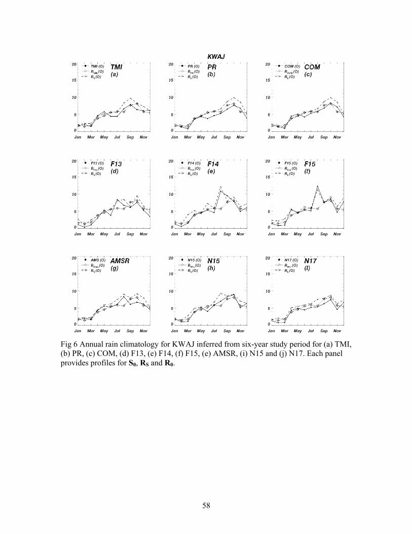
Figures 6 and 7 display the annual cycle for KWAJ and MELB for the rain
sensors listed in Table 1 using data from the six-year study period. Satellite and GV
annual climatologies were determined from monthly rain estimates for S0, RS and R0. R0,
which is independent of the satellite overpass time, provides an absolute baseline for
comparing S0 and RS. For MELB, land, ocean and coast climatologies were estimated
independently using GROF land, ocean and coast classifications.
Page 20
20
KWAJ annual satellite and GV climatologies are shown in Fig. 6. KWAJ receives
the bulk of its annual rainfall during the rainy season from about May to November. S0
and RS for each satellite are closely correlated. . For most of the sensors in Fig. 6, RS
tends to exceed S0, especially during the rainy season. This trend suggests the existence
of a negative retrieval bias relative to the GV radar-inferred estimates. We can see this
pattern clearly for the case of the three TRMM rain products shown along the top row of
Fig. 6, where there appears to be a substantial retrieval bias during the peak months of the
rainy season. The long term mean monthly statistics for R0 and RS are also reasonably
well correlated, though there are differences that tend to appear during the peak of the
rainy season.
The long-term averages for MELB shown in Fig. 7 reflect differences between the
ocean, land and coast cases. MELB-Land and MELB-Coast receive the bulk of the
annual rainfall between June and September, whereas MELB-Ocean exhibits an absolute
maximum in September during the climatological peak in tropical cyclone and easterly
wave activity. A secondary oceanic maximum in June is also observed. Differences
between land, coast and ocean are most distinct for AMSR shown in Fig. 7g (these
differences also appear in N17, which is not shown). Comparing the MELB R0-Land and
R0-Coast profiles in Fig. 7i to S0, all of the satellite sensors tend to overestimate the peak
rainfall during June, July and August. It is also interesting to note the differences between
the PR and the TMI, for both sensors sample rainfall from the same orbiting platform.
The PR tracks closely with RS for all three cases, but for the TMI, there appear to be
significant retrieval errors over land during the peak rainfall months.
Page 21
21
6. Results and Discussion
a. Error Correlation Structure
Scatter diagrams of the satellite estimates of monthly rainfall are used to
characterize the sampling (RS vs. R0) and retrieval (S0 vs. RS) errors and to evaluate the
correlation structure between the estimated and validation parameters. The relevant
validation parameters in each case are taken to represent the independent variable: R0 for
the sampling case and RS for the retrieval case. The analysis and discussion that follows
will ascribe meaning to the correlation coefficients and slope parameters determined from
linear regressions of the random variables associated with sampling and retrievals.
1) Sampling
Scatter diagrams of RS versus R0 are presented in Figs. 8 and 9 for KWAJ and
MELB for each of the rain sensors. Monthly estimates for MELB were further subdivided
into sub-categories corresponding to the GPROF land, ocean and coast surface terrain
classifications. Correlation coefficients and slope parameters were calculated for each
distribution. These are displayed in Table 4. Sampling errors were estimated by
evaluating statistical differences between sub-sampled and continuously sampled GV
radar data as described in Section 3.
Table 3 evaluates the sampling frequency for each sensor relative to the average
number of overpasses per month for a randomly selected 0.25° grid box inside of 100 km
from the GV radar. The Table shows that the TMI and PR collect significantly more
samples at MELB than at KWAJ (nearly a factor of 2 difference in number) due to
TRMM’s lower angle of inclination and its sun-asynchronous orbit. Shin and North
(1987) conducted simulations of the TRMM orbit prior to launch and found that TRMM
Page 22
22
sampling errors were reduced at higher latitudes due to increased sampling. Their
findings are consistent the results of this study.
It is also observed that the polar orbiters collected a few more samples on average
over MELB than KWAJ, but this apparent difference is due to reductions in the area of
the 0.25° grid box, which varies with latitude due to converging lines of longitude at the
poles. F14 was the only sensor with fewer observations over MELB, while over KWAJ
its sampling statistics are comparable to the other polar orbiters. This anomaly in the
MELB sampling statistics for F14 is therefore probably due to missing overpasses over
related to radar downtime.
All the scatter diagrams for KWAJ in Fig. 8 display a similar structure and are
characterized by a large range of RS values and a much narrower range of R0 values.
Table 4 indicates that RS and R0 are generally not well correlated at the monthly scale,
but the degree of correlation is sensitive to differences in the temporal and spatial
sampling characteristics of the sensor. For KWAJ, the observed inter-sensor variability
depends primary on the relative swath width of the sensor, for near to the equator the
satellite sampling frequency is nearly constant for the different satellites analyzed in this
study.
Table 4 for KWAJ indicates that the AMSU rain sensors on average exhibited the
highest correlation, while the PR/COM group displayed the lowest correlation. This
predictable result shows the dependency of the sampling error on the swath geometry of
the sensor. AMSU sweeps out a 1600 km swath width compared to a 247 km swath for
the PR. It subsequently covers an area 6.5 times larger than the PR per overpass. Slope
values for the PMW sensors (excluding PR/COM) range from 0.98 to 1.15. Discrete
Page 23
23
temporal sampling results in the satellite tending to overestimate rainfall when S0 and RS
are both high, while underestimating rainfall when S0 and RS are very low. Consequently
a small number of overestimates at the high end are compensated by a much larger
number of underestimates at the low end. Fisher (2004) observed similar results in the
long-term PDF of monthly estimates from the TMI and PR collected over Oklahoma.
Morrissey and Janowiak (1996) attributed this error correlation structure to a conditional
sampling bias in climate-scale estimates resulting from discreet temporal sampling of the
satellite. They found that the magnitude and sign of the bias depended on the mean
monthly rain rate.
Diagnosing the effects on the MELB results shown in Fig. 9 is more complex due
to differences in the land, ocean and coast sub-climate regimes. First examining the polar
orbiting PMW sensors, F13 and F14 regress appear to incur negative oceanic sampling
biases. This can be inferred from Fig. 9 together with the slope of the regression shown
in Table 4. AMSR-E, F15, N15 and N16, on the other hand, appear to incur a positive
bias. F13 and F14 were the only two satellites to display lower correlations over MELB
than KWAJ. Note F14 was the only satellite to collect fewer observations over MELB.
Over land, F14, F15 and N17 are negative, but F13, AMSR-E N15 and N16 are positive.
We also observe a significantly larger variance in the both the correlation coefficients and
slopes over land, which we attribute to sampling coupled to climate variability associated
with the amplitude and phase of the diurnal cycle for the land and coast cases.
The benefits of improved sampling are most clearly observed over MELB for the
TRMM rain estimates. The TMI and PR exhibited generally higher correlations and slope
values that approach unity for each of the three terrain cases. These improvements are
Page 24
24
attributed to both a larger number of observations and more representative sampling of
the diurnal cycle.
2) Retrievals
Scatter diagrams of S0 and RS are utilized here to examine retrieval error
characteristics. Since both rain parameters are spatio-temporally matched, it is assumed
that they observe the same distribution of instantaneous rain rates. Figures 10 and 11
present scatter diagrams of S0 and RS at KWAJ and MELB, respectively, and Table 5
lists the corresponding regression parameters. Table 5 clearly shows that S0 and RS are
more highly correlated than RS and R0. The slopes associated with each regression,
however, tended to be less than one for both KWAJ and MELB. This observation holds
for all the oceanic satellite estimates, again suggesting a positive retrieval bias over the
oceans.
The oceanic rain retrievals are of special interest for evaluating the accuracy of
the physical rain retrievals of the TMI, AMSR and SSM/I. The oceans provide a cold
radiometric surface with a distinguishable polarization signature, allowing for a
decoupling of surface emissions from those emanating from the atmosphere above. It
should be noted that AMSU-A and B channels lack polarization information and
consequently, the lower frequency emission channels on AMSU-A are not used by the
AMSU rain rate algorithm, which relies on radiometric information from the 89 and 150
GHz scattering channels on AMSU-B (other lower frequency channels on AMSU-A are
used to screen the surface, but only play an ancillary role in the determination of the rain
rate).
Page 25
25
The correlation coefficients for the rain retrievals over KWAJ and MELB-Ocean
are restricted to a similar range of values. Correlations for KWAJ range from 0.66 (F15)
to 0.91 (PR/COM), while for MELB-Ocean they range from 0.64 (F13) to 0.88 (TMI).
Slope values determined from each regression are also consistently less than one for all of
the rain sensors, revealing the presence of a negative oceanic retrieval bias. The retrieval
bias will be considered more quantitatively in the Section 7b.
For the TMI, AMSR and SSM/I, differences in the error correlation for the ocean
can be related to differences in the relative size of the FOV in the emission channels. The
FOV for the TMI and AMSR water vapor channels, for example, are about 450 km2 and
560 km2, respectively, and cover an area smaller than the area of the grid box (~750
km2). The SSM/I nominal FOV for the water vapor channel is about 2000 km2 and more
closely approximates the size of a 0.50 grid box (~3000 km2).
The larger footprint also introduces additional beam-filling effects that are
significant when sampling highly convective systems with large rain rate gradients
embedded in the rain field (Kummerow et al. 1998). Oceanic SSM/I rain retrievals
showed lower correlations and higher variance than TMI and AMSR for both KWAJ and
MELB-Ocean. These differences in the error correlations structure to first order are
attributed to the relative differences in the size of the FOV with respect to the gridding
scale of the study.
Rain retrievals over land and coast are evaluated using MELB-Land and MELB-
Coast displayed in Fig. 11. The GPROF land and coast algorithm is constrained by the
observations in the high frequency channels, corresponding to the two 85.5 GHz channels
on the TMI and SSM/I and the 89 GHz channels on AMSR. These channels have a
Page 26
26
smaller FOV than the lower frequency channels, eg., 35 km2 at 85.5 GHz compared to
400 km2 in the water vapor channel at 21.3GHz. The better resolution provides some
structural information on the rain rate gradients associated with convective systems, but
this information must be ascertained from the ice scattering signature that occurs in
higher regions of the cloud.
Correlations varied over a larger range and appear related to size differences in
the relative sensor FOVs. Over land, correlations range from 0.53 (N17) to 0.90 (COM),
whereas and over coast they range from 0.45 (N17) to 0.92 (COM). Relative differences
in the slope parameters more closely correspond to differences in the relative land, ocean
and coast climatology and the overpass times of the polar orbiting satellites.
Although AMSU has an additional high frequency channel at 150 GHz, the
AMSU group in general exhibited the lowest correlations over land and coast. AMSU
scatter diagrams suggest problems in observing higher instantaneous rain rates, which
may explain some of the large negative differences between S0 and RS. The AMSU ice
scattering algorithm may also have ancillary problems screening out surface anomalies.
The SSM/I group exhibits the most variability amongst the PMW sensors. The
TMI/AMSR group exhibits significantly higher correlations over the ocean than over
land and coast due to the addition of the low frequency rain information.
The PR/COM retrieval statistics showed the best overall performance relative to
correlation slope and also reveal a higher range of values. The PR/COM statistical
indexes also show more relatively consistency in the retrievals over land, ocean and coast
scenes. The PR has much better vertical resolution than the PMW rain sensors and
because it has a smaller FOV can better resolve strong gradients in the rain field
Page 27
27
associated with smaller scale convective rain structures. Still, the surface classification
can impact the reflectivity measurement of the PR, either due to changes in the drop size
distribution over land and ocean (assumptions about the DSD assumptions are built into
the algorithm) or to the surface reference technique applied by the PR algorithm
(Meneghini et al 2000, Iguchi et al. 2000, Robertson et al. 2003).
b. Geo-spatial Distribution of Errors and Biases
1) Sampling errors and biases
KWAJ and MELB climate-scale rain estimates were analyzed at the 0.25° grid
spacing using the error model described in Section 3. All mean error statistics were
computed inside of 100 km to avoid mixing GV rain estimates computed from different
CAPPI levels. Mean sampling errors for KWAJ are shown in Table 6 and ranged from
3.1 to 6.3 mm/day. Oceanic sampling errors for MELB spanned a lower range of values
from 2.4 to 4.8 mm/day, about 25% less than the range estimated for KWAJ. Table 6 also
suggests that for MELB sampling and retrieval errors over land are greater than over
ocean.
Differences in the oceanic sampling errors determined for KWAJ and MELB are
correlated with increased satellite sampling rates at higher latitudes. Examining Table 3,
we see that for the TMI and the PR the sampling rate increases by nearly a factor of 2 due
to the satellite’s lower angle of inclination (Shin and North 1988). For the other PMW
sensors, the number of overpasses does not increase but the grid boxes at higher latitudes
are smaller due converging line of longitude, resulting in broader coverage of the grid
box at higher latitudes.
Page 28
28
The geo-spatial distributions of the sampling errors for KWAJ and MELB are
shown in Figs. 12 and 14, respectively. Inside of 100 km, the KWAJ sampling errors for
PMW rain sensors are confined to a relatively small range of variability. Sampling errors
tend to increase beyond this range, but inside of 100 km we do not see a clear connection
between the distribution of sampling errors and the timing of the overpass. Comparing
the six panels for MELB, we observe considerable inter-sensor variability. Differences
between land, ocean and coast are evident in some of the panels but there is no clear
pattern that clearly separates the sampling errors associated with the geo-terrain mask.
The PR’s sampling errors exhibited the greatest range of variability at both sites.
Table 6 indicates that these errors are about 1/3 greater than the TMI as seen in Table 6.
Based on the mean sampling statistics listed in Table 3, the PR only collects about half as
many samples over KWAJ than for MELB. These large sampling errors limit the relative
accuracy of the PR’s climate-scale rain estimates, even though as we will see, its rain
retrievals outperform the other sensors. The PR rain estimates also not as sensitive to the
surface classification.
Mean sampling biases for KWAJ shown in Table 7a ranged from 0.35 to 1.03 mm
day-1 and were systematically positive for all the PMW sensors. Ocean biases for MELB
were also systematically positive overall, ranging from -0.48 to 0.49. For MELB, only
N16 (-0.48) and F15 (-0.04) exhibited an overall negative sampling bias. F15 and the
PR/COM exhibited the lowest long-term sampling bias for KWAJ (0.35). PR/COM
biases shown in Fig. 13 are more randomly distributed, whereas the other PMW sensors
over KWAJ are systematically positive across the entire GV domain.
Page 29
29
A stronger coupling between the sampling times and the land-coast-ocean MELB
climatology produces a more complex bias pattern for MELB shown in Fig. 15 than what
was observed for KWAJ in Fig. 13. In Fig. 15 there exists considerable inter and intra-
sensor variability. The inferred biases for the two AMSU sensors in Fig. 15, N15 biases
are mostly positive while N17 biases are mostly negative. From Fig. 3, it is tempting to
attribute this striking pattern to differences in the timing of the overpasses. N17, for
instance, does not sample the convective cycle shown Fig. 3 for MELB, whereas the
daytime overpass for N15 flies over MELB at about 18 LST. AMSR-E flies over MELB
at 1:30 LST during the peak of the convective cycle, resulting in predominantly positive
sampling biases across the GV sampling domain. The sign of the biases for F13, on the
other hand, tends to change based on the geo-terrain classification (positive over land,
negative over ocean). The sampling biases for the two TRMM sensors tended to be lower
and more randomly distributed than the other PMW sensors, as further evidenced by the
mean biases for each (0.10 mm/day for the TMI and 0.17 for the PR) .
2) Retrieval errors and biases
Bulk retrieval errors for KWAJ are shown in Table 6 and span a range between
2.1 and 3.7 mm hr-1. At the low end of this range is the TMI/AMSR group (2.1 mm hr-1),
whereas the SSM/I group is found at the high end (3.7 mm hr-1). MELB-Ocean exhibited
a slightly lower trend (1.7 to 3.3 mm hr-1), but we also observe more intra-group
variability within each sensor class. This section will focus on the sensor characteristics
and algorithmic differences in the retrievals to explain the observed errors and biases.
Page 30
30
The geo-spatial distribution of retrieval errors for KWAJ and MELB are
displayed in Figs. 16 and 18. The COM replaces N17 in the top right panel of each figure.
The retrievals errors for KWAJ tend to be isotropically distributed, with significantly
larger errors observed at distances greater than 100 from the radar. Increases in the
retrieval errors outside of 100 km are attributed to greater uncertainties in the GV radar
estimates due to the sudden shift from the 1.5 to 3.0 km CAPPI. This shift in CAPPI
levels was previously described in Section 4. At KWAJ there is no gauge information
beyond 80 km to calibrate rain rates estimated from the 3.0 km CAPPI. Although there is
some residual range dependency observed at MELB as well where gauge stations exist
out to 150 km, range effects probably contribute less to the variability than other factors
such as differences in surface terrain (Note since there exists no gauge information over
the Atlantic Ocean east of the GV radar, oceanic rain rates must be calibrated using the
gauge PDF over land).
Mean retrieval biases for KWAJ and MELB are shown in Table 7b. All of the
oceanic rain estimates for KWAJ exhibit large biases ranging from -1.93 to -0.93
mm/day. The geo-spatial distribution of biases shown in Fig. 17 shows a relatively
homogenous distribution of negative retrieval biases throughout the GV domain, with
some tendency for larger biases in the far southern quadrant. Oceanic retrieval biases for
MELB also tended to be negatively skewed, but occur within a lower range (-0.92 to
0.08). The geo-spatial distribution of biases for PMW sensors shown in Fig. 19 shows a
strong dependency on the terrain type and the coupling of the satellite orbit to the
sampling of the climatology.
Page 31
31
Negative oceanic retrieval biases for TMI, AMSR and SSM/I are partly attributed
to beam filling in the low frequency emission channels and partly attributed to saturation
of the channels at high rain rates (Ha and North 1994, Kummerow 1998). Beam filling
tends to smear the peak rain rates of the smaller convective cells over the whole FOV.
Saturation places unphysical constraints on the maximum observable rain rate. AMSU
oceanic rain rates on the other hand are determined using a pure scattering algorithm that
only utilizes high frequency rain information and consequently are less correlated with
the integrated water content at the cloud base. The PR has the smallest FOV of all the
sensors examined and is better suited for detecting the peak rain rates associated with
small-scale convective cells, but the PR also has to account for the two-way attenuation
due to the intervening water and ice in the observed cloud system (Meneghini, 2000).
The mean oceanic sampling and retrieval biases in Table 7a and 7b tend to exhibit
opposite signs. This same pattern is also observed in Figs. 13, 15, 17 and 19 for both
KWAJ and MELB, which effectively reduces the overall bias in the rain estimate. As
noted in Section 4, it is expected that there will be some mixing of sampling and retrieval
biases due to the fact RS always fills the entire grid box, while S0 does not necessarily fill
the box, we do not consider this an explanation for the differences observed. Error mixing
in this case should be a random effect that should lead to increased variability – through
under and over estimates relative to a correctly weighted S0 – but should not have a large
effect on the long-term mean statistics. Consequently, we relate differences in the
sampling and retrieval biases to fundamental differences in the structure of the sampling
and retrieval distributions characterized in the scatter diagrams shown in Figs. 8-11.
Page 32
32
MELB retrieval errors characterized in Table 6 tended to increase appreciably
over land and coast relative to ocean when compared to the results computed for each
sensor. TMI/AMSR bulk errors for MELB are nearly the same over the ocean, but the
TMI retrieval errors over land and coast were considerably lower than AMSR. The TMI
and AMSR have similar instrument characteristics and determine rain rates using the
GPROF rain algorithm. We subsequently relate the more salient differences over land
and coast to increased variability in the diurnal rain rate statistics for AMSR due to
differences in the sampling times of each satellite. AMSR flies over MELB at
approximately 0130 and 1330 LST each day, where TRMM precesses through the diurnal
cycle at different times. AMSR is subsequently more likely to observe higher convective
rain rates during the early afternoon overpass. Similar reasoning can be applied to explain
intra-group differences observed for SSM/I and AMSU.
More salient inter- and intra-sensor differences in the satellite retrievals appear in
the bias fields for MELB shown in Fig. 19. N15 tends to exhibit positive retrieval biases
over land and negative biases over the ocean. These two bias “regimes” are partitioned
according to the location of the Florida coastline. F13, in contrast, displays a large swath
of positive coastal biases that straddle the Florida coastline. This same pattern was
observed in F14 and F15 as well (but this data was only available through 2006). We
attribute this distinguishable feature to factors associated with the instrument
characteristics and larger FOV of the SSM/I, and not to differences in overpass times.
7. Conclusions
Regional sampling and retrieval errors in monthly rainfall were statistically
estimated for five different microwave sensors on board eight orbiting satellites using six-
Page 33
33
years of instantaneous satellite rain measurements collected over Kwajalein and
Melbourne, Florida. Instantaneous ground-based radar rain estimates were used to sub-
sample the data during satellite overpasses to decouple the sampling and retrieval errors
from the total monthly error budget as described in Section 3.
Satellite and GV climatologies constructed from the data sets showed that the
satellite rain estimates were highly correlated with GV rain estimates sub-sampled during
satellite overpasses, and GV sub-sampled rain estimates, moreover, resolved most of the
fine structure observed in the satellite climatologies. This empirical methodology,
however, will tend to overestimate the satellite sampling error due to intermittent radar
downtime at times when the satellite is overhead by reducing the effective number of
matching overpasses relative to actual number of times the satellite flies over the site.
Radar downtime, however, should not affect the assessment of the retrieval errors.
Furthermore, the quantitative assessment of satellite sampling errors still provides a
relative measure for evaluating the different sampling designs and provides an absolute
baseline for assessing the impact of sampling errors on the long-term rain estimates.
Long-term sampling errors, as expected, were closely linked to the swath area of
the rain sensor and the sampling frequency of the satellite, while sampling biases were
more closely associated with the coupling of the sampling times to the diurnal
climatology associated with each GV site. The TRMM satellite orbit collected more
samples over MELB than KWAJ, which resulted in a significant reduction in the TMI
and PR sampling errors over MELB Ocean relative to KWAJ. The polar orbiting
satellites also showed some reduction in the sampling errors over MELB Ocean due in
part to a ~13% reduction in the area of the 0.25° grid box at the higher latitude. For
Page 34
34
evaluating oceanic rainfall trends, the relative benefits of the TRMM orbit in reducing
random sampling errors and biases were marginal compared to the polar orbiting
satellites.
The TRMM sensors, however, did show lower sampling biases over MELB Land
and Coast where the diurnal cycle exhibits a large amplitude during the afternoon hours.
For these two cases, the two TRMM sensors provided significantly less biased rainfall
estimates due to TRMM’s asynchronous orbit. For the polar orbiting sensors, the
sampling biases over Land and Coast were mixed and were sensitive to the overpass
times relative to the phase of the diurnal cycle. The benefits of the TRMM sampling
design were much less clear over oceanic surfaces, where a low amplitude diurnal cycle
prevailed. Overall, positive long-term sampling biases were observed at KWAJ for all of
the sensors, and similarly, positive oceanic sampling biases were observed for most of the
sensors at MELB.
All of the rain estimates tended to exhibit negative retrieval errors over ocean
surfaces by between 10 and 30% relative to the two GV radars. This important result was
observed over both KWAJ (all ocean) and MELB Ocean and appears to be a significant
issue for the algorithm developers. Inter-sensor differences in the retrieval biases were
most prominent for MELB where there exists a strong coupling between the diurnal cycle
and the satellite sampling times. This study did not attempt to quantify seasonal
variations in the error characteristics, but direct comparisons of satellite and GV annual
climatologies, along with previous studies by McCollum et al. (2002) and Fisher (2007),
suggest that the PMW rain algorithms may not be adequately handling seasonal changes
in the microphysical properties of rainfall.
Page 35
35
The SSM/I, TMI and AMSR-E monthly rain retrievals utilize both emission and
scattering channels over ocean surfaces, whereas AMSU only utilizes high frequency
scattering channels, which are less correlated with surface rainfall. Based on satellite
comparisons with the GV oceanic estimates, SSMI/I, TMI and AMSR-E, tended to yield
higher correlations with ground estimates relative to AMSU. Results from the error
analysis were somewhat mixed but the TMI/AMSR-E group did tend to exhibit smaller
retrieval errors over ocean.
The PR/COM group exhibited the highest correlations with the ground-based
radars and the rain retrievals were less dependent on the characteristics of the surface
classification. Although the PR outperformed most of the PMW rain sensors, its poor
sampling statistics limits its potential for monitoring long-term rainfall trends. However,
as can be seen from an examination of the error and bias characteristics of the COM, he
PR provides important rain information for improving the rainfall estimates associated
with the microwave retrievals and for diagnosing the internal structure of individual rain
systems.
Page 36
36
References
Bell T. L., and N. Reid, 1993: Detecting the Diurnal Cycle of Rainfall Using Satellite
Observations. J. Appl. Meteor., 32, 311-322.
Bell T. L., and P. K. Kundu, 2000: Dependence of satellite sampling error on monthly
averaged rain rates: comparison of simple models and recent studies. J. Appl.
Meteor., 13, 449-462.
Bell, T. L., P. K. Kundu, and C. D. Kummerow, 2001: Sampling errors of SSM/I and
TRMM rainfall averages: comparison with error estimates from surface data. J. Appl.
Meteor., 40, 938-954.
Fisher, B. L., 2007: Statistical error decomposition of regional-scale climatological
precipitation estimates from the Tropical Rainfall Measuring Mission (TRMM). J.
Appl. Meteor. and Climatol., 46, 791-813.
Fisher, B. L., 2004: Climatological validation of TRMM TMI and PR monthly rain
products over Oklahoma. J. Appl. Meteor., 43, 519-535.
40, 1801-1820.
Ha, E.,, and G. R. North, 1995: Model studies of the beam-filling error for rain-rate
retrieval with microwave radiometers. J. Appl. Meteor., 12, 268-281.
Haddad, Z., E. Im, S. L. Durden, and S. Henly, 1996: Stochastic filtering of rain profiles
using radar, surface-referenced radar, or combined radar-radiometer measurements. J.
Appl. Meteor., 35, 229-242.
Kongoli, C., R. R. Ferraro, P. Pellegrino, H. Meng and C. Dean, 2007: The utilization of
the AMSU high frequency measurements for improved coastal rain retrievals.
Geophys. Res. Lett., 34, L17809, doi:10.1029/2007GL029940.
Page 37
37
Kummerow, C.W., and Coauthors, 2001: The evolution of the Goddard Profiling
Algorithm (GPROF) for rainfall estimation from Passive Microwave Sensors. J. Appl.
Meteor., 40, 1801-1820.
Kummerow, C. W. Barnes, T. Kozu, J. Shiue, J. Simpson, 1998: The tropical rainfall
measuring mission (TRMM) sensor package. J. Atmos. Oceanic Technol., 15, 809-
817.
Laughlin, C. R., 1981: On the effect of temporal sampling on the observation of mean
rainfall. Precipitation Measurements from Space, D. Atlas and O. Thiele, Eds.,
NASA Publication, D59-D66.
McCollum, J. R., W. F. Krajewski, R. R. Ferraro, M. B. Ba, 2002: Evaluation of biases of
satellite rainfall estimation algorithms over the continental United States, J. Appl.
Meteor., 41, 1065-1080.
McConnell, A., and G. North, 1987: Sampling errors in satellite estimates of tropical rain.
J. Geophys. Res., 92, 9567-9570.
Meneghini, R., T. Iguchi, T. Kozu, L. Liao, K. Okamoto, J. A. Jones, J., Kwiatkowski,
2000: Use of the surface reference technique for path attenuation estimates from the
TRMM precipitation radar. J. Appl. Meteor., 39, 2053-2070.
Morrissey, M. L., and J. E. Janowiak, 1996: Sampling-induced conditional biases in
satellite climate-scale rainfall estimates, J. Appl. Meteor., 35, 541-548.
Negri, A., J., T. L. Bell and L. Xu, 2002: Sampling of the Diurnal Cycle. J. Appl.
Meteor., 19, 1333-1344.
North, G .R., 1988: Survey of sampling problems for TRMM. Tropical Rainfall
Measurements, J. S. Theon and N. Fugono, A. Deepak Publ., 337-348.
Page 38
38
Oki, R., and A. Sumi, 1994: Sampling simulation of TRMM rainfall estimation using
radar-AMeDAS composites. J Appl. Meteor., 33, 1597-1608.
Olson, W. S., and Co-authors, 2006: Precipitation and latent heating distributions from
satellite passive microwave radiometry. Part I: Improved method and uncertainty
estimates. J. Appl. Meteor., 702-720.
Qiu, S., P. Pellegrino, R. Ferraro, and L. Zhao, 2005: The improved AMSU rain-rate
algorithm and its evaluation for a cool season event in the western United States.
Wea. Forecasting, 20, 761–774.
Robertson, F. R., D. E. Fizjarrald, C. D. Kummerow, 2003: Effects of uncertainty in
TRMM precipitation radar path integrated attenuation on interannual variations of
tropical oceanic rainfall. Geophys. Res. Lett., 30, 50 doi: 10.1029/2002GL016416.
Salby M. L., and P. Callaghan. 1997: Sampling error in climate properties derived from
satellite measurements: consequences of undersampled diurnal variability. J. Climate,
10, 18-36.
Shin, K., and G. R. North, 1988: Sampling error study for rainfall estimate by satellite
using a stochastic model. J. Appl. Meteor., 27, 1218-1231.
Shin, K., G. R. North, Y. Ahn, and P. A. Arkin, 1990: Times scales and variability of
area-averaged tropical oceanic rainfall. J. Appl. Meteor., 118, 1507-1516.
Spencer, R. W., H. M. Goodman, and R. E. Hood, 1989: Precipitation retrieval over land
and ocean with the SSM/I. Part I: Identification and characteristics of the scattering
signal. J. Atmos. Ocean. Tech., 6, 254-273.
Page 39
39
Steiner, M. T. L. Bell, Y. Zhang and E. F. Wood, 2003: Comparison of two methods for
estimating the sampling-related uncertainty of satellite rainfall averages based on a
large radar dataset. Journal of Climate, 16, 3759–3778.
Weng, F., L. Zhao, R. Ferraro, G. Poe, X. Li, and N. Grody, 2003: Advanced Microwave
Sounding Unit cloud and precipitation algorithms. Radio Sci., 38, 8068-8079.
Wilheit, T. T., 1988: Error analysis for the Tropical Rainfall Measuring Mission
(TRMM). Tropical Rainfall Measurements, J. S. Theon and N. Fugono, Eds., A.
Deepak Publishing, 377-385.
Wolff, D. B., and B. L. Fisher, 2009: Assessing the relative performance of microwave-
based satellite rain-rate retrievals using TRMM ground validation data. J. Appl.
Meteor., 48, 1069-1099.
Wolff, D. B., D. A. Marks, E. Amitai, D. S. Silberstein, B. L. Fisher, A. Tokay, J.
Wang, and J. L. Pippitt, 2005: Ground validation for the Tropical Rainfall
Measuring Mission (TRMM). J. Atmos. Oceanic Technol., 22, 365-380.
Wright, Tom, 2006: Tropical storm Talas formation and impacts at Kwajalein Atoll, 27th
Conf. on Hurricanes and Tropical Meteor., J16A.3.
Page 40
40
TABLE CAPTIONS
TABLE 1 Instrument and orbital characteristics for the eight satellites and five rain
sensors used in the study.
TABLE 2. Radar Downtime.
TABLE 3. Mean Sampling Frequency per Month.
TABLE 4. Correlations coefficients and slopes of linear regressions characterizing the
relationship between RS and R0
TABLE 5. Correlations coefficients and slopes of linear regressions characterizing the
relationship between S0 and RS
TABLE 6. Summary sampling and retrieval error statistics for KWAJ and MELB
stratified by the GPROF surface terrain classification (land, ocean or coast).
TABLE 7a. Sampling bias statistics for KWAJ and MELB.
TABLE 7b. Retrieval bias statistics for KWAJ and MELB.
Page 41
41
FIGURE CAPTIONS
Fig. 1. The top half the figure a) illustrates the process of discrete temporal sampling. The
left side of 1a) represents the entire spatio-temporal domain of the sampled region A. The
right side of 1a) shows the sequence of discrete snapshots collected at overpasses
separated by time intervals, Δt. The lower half of the figure 1b) illustrates the retrieval
process for the TRMM satellite. The TMI and PR retrieve rainfall information from area
A for the region defined by the swath of each sensor. The footprint of each sensor
subsequently determines the resolution of the measurement. Although the TMI and PR
both obtain snapshots of A at Δt, the PR incurs larger sampling errors due to differences
in the area of the swath.
Fig. 2 Top two panels display site maps for KWAJ (top left) and MELB (top right).
Range rings are shown out to 200 km. Rain gauge locations are also shown. The lower
two panels display the GPROF surface terrain mask for KWAJ (lower left) and MELB
(lower right)
Fig 3 Mean diurnal cycle for KWAJ (top) and MELB (bottom) computed during the
study period as a function of the hour. Each polar orbiting satellite is represented by a
unique symbol shown in the legend showing the two times when the satellite flies over
the GV site.
Page 42
42
FIG. 4 Equator crossing times during the lifetime of the satellites analyzed in the study.
The dotted vertical lines enclose the study period from 2003 to 2008. The row of times
shown at the bottom of the figure represents the total temporal drift during the study
period.
Fig 5 Diurnal rain climatology for KWAJ and MELB estimated for the six-year study
period using the TRMM rain products (TMI, PR and COM). The four panels compare
rain profiles for S0, RS and R0. Each profile has been normalized based on the total
rainfall over the 24-hour period.
FIG. 6 Annual rain climatology for KWAJ inferred from six-year study period for (a)
TMI, (b) PR, (c) COM, (d) F13, (e) F14, (f) F15, (e) AMSR, (i) N15 and (j) N17. Each
panel provides profiles for S0, RS and R0.
FIG. 7 Annual rain climatology for MELB inferred from six-year study period for for (a)
TMI, (b) PR, (c) COM, (d) F13, (e) F14, (f) F15, (e) AMSR, (i) N15 and (j) R0. The
lower right panel (j) represents the true rain climatology based on R0 as stratified by land,
ocean and coast. The other panels represent the inferred climatology based on the S0 and
RS, which have been further stratified based on the surface criteria.
FIG. 8 Scatter plots for KWAJ computed at 0.25° inter-comparing RS and R0 monthly
estimates.
Page 43
43
FIG. 9 Scatter plots for MELB computed at 0.25° inter-comparing RS and R0 monthly
estimates land (solid line, open circles), ocean (dash-dot line, triangles) and coast (dashed
line, plus sign) cases.
FIG. 10 Scatter plots for KWAJ computed at 0.25° inter-comparing S0 and RS monthly
estimates.
FIG. 11 Scatter plots for MELB computed at 0.25° inter-comparing S0 and RS monthly
estimates for the land (solid line, open circles), ocean (dash-dot line, triangles) and coast
(dashed line, plus sign) cases.
FIG. 12 Geographical distribution of sampling errors in mm day-1 for KWAJ considered
for the entire study period (2003-2008).
FIG. 13 Geographical distribution of sampling biases for KWAJ considered for the entire
study period (2003-2008).
FIG. 14 Geographical distribution of sampling errors for MELB in mm day-1 considered
for the entire study period (2003-2008).
Page 44
44
FIG. 15 Geographical distribution of sampling biases for MELB considered for the entire
study period (2003-2008).
FIG. 16 Geographical distribution of retrieval errors for KWAJ in mm day-1 considered
for the entire study period (2003-2008).
FIG. 17 Geographical distribution of retrieval biases for KWAJ considered for the entire
study period (2003-2008).
FIG. 18 Geographical distribution of retrieval errors for MELB in mm day-1 considered
for the entire study period (2003-2008).
FIG. 19 Geographical distribution of retrieval biases for MELB considered for the entire
study period (2003-2008).
Page 45
45
TABLE 1. Instrument and orbital characteristics for the eight satellites and five rain sensors used in the study. Satellite Agency
Sponsor Sensor Type
Launch (Yr/Mon)
No. Chan.
Freq. Range (GHz)
Swath Width (Km)
Altitude (Km)
F13 DMPS SSM/I 1997/03 7 19-85.5 1400 830 F14 DMPS SSM/I 1997/05 7 19-85.5 1400 830 F15 DMPS SSM/I 1999/12 7 19-85.5 1400 830 N15 NOAA AMSU-B 1998/05 5 89 – 183 1600 830 N16 NOAA AMSU-B 2000/09 5 89 – 183 1600 830 N17 NOAA AMSU-B 2002/06 5 89 – 183 1600 830 Aqua NASA AMSR-E 2002/05 12 6.9 – 89 1445 705
TRMM NASA TMI 1997/11 9 10 – 85.5 759 402 TRMM NASA PR 1997/11 N/A 13.8* 215 402 TRMM NASA COM 1997/11 N/A TMI/PR^ 215 402
* Active precipitation radar ^Hybrid rain product that combines the rain information from the TMI and PR.
Page 46
46
TABLE 2. Radar Downtime KWAJ MELB
Year Radar down for more than 4 hours in day (days/year)
Mean Radar down time
(days/month)
Radar down for more than 4 hours in day (days/year)
Mean Radar down time
(days/month)
2003 32 2.7 12 1.0 2004 36 3.0 56 4.7 2005 19 1.6 34 5.7* 2006 26 2.2 48 4.0* 2007 18 1.5 42 3.5 2008 11 0.9 11 1.2*
• averages computed based on fewer than 12 months
Page 47
47
TABLE 3. Mean Sampling Frequency per Month. Mean Sampling Frequency
(Samples/Month) Satellite KWAJ MELB F13 30.5 32 F14 28 24 F15 29 32 N15 45 49 N16 49 53 N17 45 49 AMSR 31 35 TMI 34 62 PR 10.5 19 COM 10.5 19
Page 48
48
TABLE 4. Correlations coefficients and slopes of linear regressions characterizing the relationship between RS and R0
KWAJ MELB Satellite Ocean Land Ocean Coast Cor. Slope Cor. Slope Cor. Slope Cor. Slope F13 0.49 0.98 0.55 1.14 0.36 0.56 0.44 0.97 F14 0.48 1.07 0.29 0.47 0.45 0.69 0.33 0.62 F15 0.47 1.00 0.31 0.51 0.71 1.10 0.51 0.88 N15 0.60 1.03 0.69 1.40 0.74 1.05 0.67 1.11 N16 0.67 1.15 0.76 1.53 0.77 1.03 0.70 1.29 N17 0.60 1.00 0.53 0.55 0.76 1.14 0.62 0.70 AMSR 0.55 1.03 0.52 1.35 0.58 1.12 0.60 1.37 TMI 0.52 0.98 0.63 1.01 0.78 1.12 0.67 1.06 PR/COM 0.30 0.88 0.39 0.98 0.48 1.08 0.44 0.97
Page 49
49
TABLE 5. Correlations coefficients and slopes of linear regressions characterizing the relationship between S0 and RS
KWAJ MELB Satellite Ocean Land Ocean Coast Cor. Slope Cor. Slope Cor. Slope Cor. Slope F13 0.71 0.71 0.66 0.86 0.68 0.68 0.90 0.90 F14 0.70 0.70 0.66 0.89 0.70 0.81 0.74 1.42 F15 0.66 0.69 0.63 0.60 0.73 0.80 0.69 0.93 N15 0.74 0.66 0.69 0.86 0.68 0.67 0.56 0.68 N16 0.75 0.64 0.56 0.68 0.74 0.70 0.66 0.61 N17 0.71 0.56 0.53 0.68 0.53 0.68 0.45 0.63 AMSR 0.87 0.71 0.74 0.72 0.88 0.72 0.78 0.79 TMI 0.87 0.77 0.81 1.04 0.88 0.72 0.78 0.75 PR 0.91 0.75 0.88 0.72 0.86 0.88 0.90 0.78 COM 0.91 0.69 0.90 1.06 0.83 0.95 0.92 0.96
Page 50
50
TABLE 6. Summary sampling and retrieval error statistics for KWAJ and MELB stratified by the GPROF surface terrain classification (land, ocean or coast).
Sampling Errors (mm/day) Retrieval Errors (mm/day) KWAJ MELB KWAJ MELB
Satellite
Ocean Land Ocean Coast Ocean Land Ocean Coast F13 4.1 3.9 3.6 3.5 3.5 4.0 2.9 4.4 F14 4.4 3.4 3.4 4.1 3.7 3.5 3.0 4.7 F15 4.3 2.9 2.8 3.2 3.7 2.6 2.6 3.0 N15 3.4 3.4 2.4 2.7 2.8 4.0 2.7 3.4 N16 3.1 3.3 2.5 3.1 2.8 2.9 2.6 3.0 N17 3.2 2.0 2.6 2.2 2.8 3.4 3.3 2.4 AMSR 3.9 4.2 3.3 3.8 2.1 3.6 2.0 3.2 TMI 4.0 2.9 2.4 2.7 2.1 2.6 1.7 2.3 PR 6.3 5.0 4.8 4.3 2.7 2.4 2.8 2.0 COM 6.3 5.0 4.8 4.3 2.7 2.7 3.2 2.0
Page 51
51
TABLE 7a: Sampling bias statistics for KWAJ and MELB. Sampling Biases
KWAJ MELB Ocean Land Ocean Coast
Satellite
rsb msb rsb msb rsb msb rsb msb F13 0.10 0.49 0.22 0.68 0.05 0.17 0.02 0.05 F14 0.15 0.71 -0.25 -0.81 0.04 0.12 -0.15 -0.45 F15 0.07 0.35 -0.22 -0.69 -0.01 -0.04 -0.12 -0.35 N15 0.21 0.97 0.42 1.31 0.12 0.38 0.18 0.54 N16 0.22 1.03 0.17 0.51 -0.15 -0.48 0.09 0.25 N17 0.12 0.56 -0.35 -1.09 0.00 0.01 -0.26 -0.77 AMSR 0.17 0.79 0.20 0.61 0.09 0.28 0.25 0.73 TMI 0.17 0.77 0.03 0.10 0.07 0.24 0.06 0.18 PR 0.08 0.35 0.06 0.18 0.15 0.49 -0.05 -0.15 COM 0.08 0.35 0.06 0.18 0.15 0.49 -0.05 -0.15
Page 52
52
TABLE 7b: Retrieval bias statistics for KWAJ and MELB Retrieval Biases
KWAJ MELB Ocean Land Ocean Coast
Satellite
rrb mrb rrb mrb rrb mrb rrb mrb F13 -0.29 -1.47 0.18 0.68 -0.11 -0.40 0.48 1.48 F14 -0.33 -1.83 0.14 0.34 -0.18 -0.61 0.67 1.73 F15 -0.37 -1.93 0.12 0.29 -0.05 -0.17 0.48 1.27 N15 -0.24 -1.34 0.15 0.68 -0.10 -0.38 0.00 0.01 N16 -0.32 -1.82 -0.09 -0.35 -0.21 -0.58 -0.19 -0.63 N17 -0.31 -1.61 -0.20 -0.41 -0.28 -0.92 -0.42 -0.93 AMSR -0.24 -1.32 -0.02 -0.07 -0.08 -0.27 -0.07 -0.25 TMI -0.23 -1.24 0.13 0.43 -0.13 -0.45 -0.13 -0.41 PR -0.29 -1.46 -0.08 -0.26 -0.10 -0.36 -0.07 -0.26 COM -0.18 -0.93 0.23 0.75 0.02 0.08 0.17 0.48
Page 53
53
Fig. 1. The top half the figure a) illustrates the process of discrete temporal sampling. The left side of 1a) represents the entire spatio-temporal domain of the sampled region A. The right side of 1a) shows the sequence of discrete snapshots collected at overpasses separated by time intervals, Δt. The lower half of the figure 1b) illustrates the retrieval process for the TRMM satellite. The TMI and PR retrieve rainfall information from area A for the region defined by the swath of each sensor. The footprint of each sensor subsequently determines the resolution of the measurement. Although the TMI and PR both obtain snapshots of A at Δt, the PR incurs larger sampling errors due to differences in the area of the swath.
!"
#
!!t"
$%&"
A!A!
$'&"
TMI!PR!
#()"*+%,-"
./0"12"34"*+%,-"
56/"12"
Page 54
54
Fig. 2 Top two panels display site maps for KWAJ (top left) and MELB (top right). Range rings are shown out to 200 km. Rain gauge locations are also shown. The lower two panels display the GPROF surface terrain mask for KWAJ (lower left) and MELB (lower right)
Page 55
55
Fig 3 Mean diurnal cycle for KWAJ (top) and MELB (bottom) computed during the study period as a function of the hour. Each polar orbiting satellite is represented by a unique symbol shown in the legend showing the two times when the satellite flies over the GV site.
0.0
1.0
2.0
3.0
4.0
5.0
6.0
7.0
8.0
0 5 10 15 20
AMSR
F13
F14
F15
N15
N16
N17
mm
/hr
KWAJ
0.0
1.0
2.0
3.0
4.0
5.0
6.0
7.0
8.0
0 5 10 15 20
AMSR
F13
F14
F15
N15
N16
N 17
mm
/hr
LST
MELB
Page 56
56
Fig 4 Equator crossing times during the lifetime of the satellites analyzed in the study. The dotted vertical lines enclose the study period from 2003 to 2008. The row of times displayed at the bottom of the figure represents the total temporal drift during the study period.
Page 57
57
Fig 5 Diurnal rain climatology for KWAJ and MELB estimated for the six-year study period using the TRMM rain products (TMI, PR and COM). The four panels compare rain profiles for S0, RS and R0. Each profile has been normalized based on the total rainfall over the 24-hour period.
0.00
0.05
0.10
0.15
0.20
0.25
0 2 4 6 8 10 12 14 16 18 20 22
KWAJ/OCEAN
PR
TMI
COM
RPR
RTMI
R0
LST
0.0
0.050
0.10
0.15
0.20
0.25
0 2 4 6 8 10 12 14 16 18 20 22
MELB/OCEAN
PR
TMI
COM
RPR
RTMI
R0
LST
0.0
0.050
0.10
0.15
0.20
0.25
0 2 4 6 8 10 12 14 16 18 20 22
MELB/LAND
PR
TMI
COM
RPR
RTMI
R0
LST
0.0
0.050
0.10
0.15
0.20
0.25
0 2 4 6 8 10 12 14 16 18 20 22
MELB/COAST
PR
TMI
COM
RPR
RTMI
R0
LST
Page 58
58
Fig 6 Annual rain climatology for KWAJ inferred from six-year study period for (a) TMI, (b) PR, (c) COM, (d) F13, (e) F14, (f) F15, (e) AMSR, (i) N15 and (j) N17. Each panel provides profiles for S0, RS and R0.
Page 59
59
Fig 7 Annual rain climatology for MELB inferred from six-year study period for for (a) TMI, (b) PR, (c) COM, (d) F13, (e) F14, (f) F15, (e) AMSR, (i) N15 and (j) R0. The lower right panel (j) represents the true rain climatology based on R0 as stratified by land, ocean and coast. The other panels represent the inferred climatology based on the S0 and RS, which have been further stratified based on the surface criteria.
Page 60
60
Fig 8 Scatter plots for KWAJ computed at 0.25° inter-comparing RS and R0 monthly estimates.
Page 61
61
Fig 9 Scatter plots for MELB computed at 0.25° inter-comparing RS and R0 monthly estimates land (solid line, open circles), ocean (dash-dot line, triangles) and coast (dashed line, plus sign) cases.
Page 62
62
Fig 10 Scatter plots for KWAJ computed at 0.25° inter-comparing S0 and RS monthly estimates.
Page 63
63
Fig 11 Scatter plots for MELB computed at 0.25° inter-comparing S0 and RS monthly estimates for the land (solid line, open circles), ocean (dash-dot line, triangles) and coast (dashed line, plus sign) cases.
Page 64
64
Fig 12 Geographical distribution of sampling errors in mm day-1 for KWAJ considered for the entire study period (2003-2008).
Page 65
65
Fig 13 Geographical distribution of sampling biases for KWAJ considered for the entire study period (2003-2008).
Page 66
66
Fig 14 Geographical distribution of sampling errors for MELB in mm day-1 considered for the entire study period (2003-2008).
Page 67
67
Fig 15 Geographical distribution of sampling biases for MELB considered for the entire study period (2003-2008).
Page 68
68
Fig 16 Geographical distribution of retrieval errors for KWAJ in mm day-1 considered for the entire study period (2003-2008).
Page 69
69
Fig 17 Geographical distribution of retrieval biases for KWAJ considered for the entire study period (2003-2008).
Page 70
70
Fig 18 Geographical distribution of retrieval errors for MELB in mm day-1 considered for the entire study period (2003-2008).
Page 71
71
Fig 19 Geographical distribution of retrieval biases for MELB considered for the entire study period (2003-2008).