Page 1
This is an author produced version of a paper published in Scandinavian Journal of Forest Research. This paper has been peer-reviewed but may not include the final publisher proof-corrections or pagination.
Citation for the published paper: Rami Saad, Jörgen Wallerman and Tomas Lämås. (2015) Estimating stem diameter distributions from airborne laser scanning data and their effects on long term forest management planning. Scandinavian Journal of Forest Research. Volume: 30, Number: 2, pp 186-196. http://dx.doi.org/10.1080/02827581.2014.978888.
Access to the published version may require journal subscription. Published with permission from: Taylor & Francis.
Standard set statement from the publisher: This is an Accepted Manuscript of an article published by Taylor & Francis in Scandinavian Journal of
Forest Research on 24 nov 2014 (online), available online:
http://wwww.tandfonline.com/10.1080/02827581.2014.978888
Epsilon Open Archive http://epsilon.slu.se
Page 2
R. Saad et al. Scand. J. For. Res., 2014
RESEARCH ARTICLE 1
Estimating stem diameter distributions from airborne laser scanning data and their effects on 2
long term forest management planning 3
Rami Saad a*, Jörgen Wallerman a, Tomas Lämås a 4
*Corresponding author. Email: [email protected] 5
a Department of Forest Resource Management, Swedish University of Agricultural 6
Sciences, Umeå, Sweden 7
Abstract 8
Data obtained from airborne laser scanning (ALS) are frequently used for acquiring forest data. 9
Using a relatively low number of laser pulses per unit area (≤ 5 pulses per m2), this technique is 10
typically used to estimate stand mean values. In this study stand diameter distributions were 11
also estimated, with the aim of improving the information available for effective forest 12
management and planning. Plot level forest data, such as stem number and mean height, 13
together with diameter distributions in the form of Weibull distributions, were estimated using 14
ALS data. Stand-wise tree lists were then estimated. These estimations were compared to data 15
obtained from a field survey of 124 stands in northern Sweden. In each stand an average of 16
seven sample plots (radius 5-10 m) were systematically sampled. The ALS approach was then 17
compared to a mean value approach where only mean values are estimated and tree lists are 18
simulated using a forest decision support system (DSS). The ALS approach provided a better 19
match to observed diameter distributions: ca. 35% lower error indices used as a measure 20
1
Page 3
R. Saad et al. Scand. J. For. Res., 2014
of accuracy and these results are in line with the previous studies. Moreover – which is unique 21
compared to earlier studies – suboptimal losses were assessed. Using the Heureka DSS the 22
suboptimal losses in terms of net present value due to erroneous decisions were compared. 23
Although no large difference was found, the ALS approach showed smaller suboptimal loss than 24
the mean value approach. 25
Keywords: forest management planning, suboptimal loss, Weibull distribution, Airborne Laser 26
Scanning, Heureka, decision support system 27
28
Introduction 29
In forest planning, different potential management actions are analyzed and the actions best 30
fulfilling stated goals are chosen by the forest owner or a decision maker. The analyses and 31
decisions are based upon various characteristics of the particular stands within a forest 32
property such as timber volume, basal area and mean tree height. These forest variables are 33
used as inputs in decision support systems (DSS), such as the Swedish Heureka system 34
(Wikström et al. 2011), to simulate and evaluate different possible treatments. The outcome 35
from these systems is a management proposal for each individual forest stand, which aims to 36
maximize the utility of the forest holding. Utility is often expressed as an economic yield, 37
typically in terms of net present value (NPV) within a set of constraints based on, e.g., timber 38
flows and environmental factors. 39
40
Naturally the accuracy of forestland data affects the scope for efficient management planning, 41
therefore evaluating the quality of the available information is a critical step in forest 42
2
Page 4
R. Saad et al. Scand. J. For. Res., 2014
management (Kangas 2010). In general statistical terms the quality of the data is defined as 43
how far the available data are from the true value (accuracy). The forest information is usually 44
gathered by sample-based surveying, visual estimations (ocular standwise field inventory) or 45
remote sensing techniques such as airborne laser scanning (ALS) (McRoberts et al. 2010). 46
Estimates gathered by visual estimation tends to include both random and systematic errors, 47
while estimates from sample based surveys remote sensing can be expected to contain random 48
errors only (estimates based on remote sensing data may contain systematic errors from 49
different factors such as model lack of fit). Loss occurring from suboptimal decisions due to 50
erroneous estimates is defined as the difference between NPV based on accurate data and that 51
based on erroneous estimates on the same forest (Holmström et al. 2003). A method for 52
maximizing the utility of available data is cost-plus-loss analysis, in which the accuracy level is 53
chosen such that it minimizes the sum of direct inventory costs and the losses resulting from 54
inaccurate data (Kangas 2010). 55
56
Forest information compiled in stand register databases tends to consist of stand-level values 57
such as stem number, mean age and mean tree size. Given that DSSs typically use individual 58
tree models in their calculations, models are required to simulate tree lists from the stand 59
mean values contained in the register databases, as with the Heureka system. It is of interest to 60
use directly estimated tree list data, such as those obtained from sample plot surveys, in order 61
to avoid the inherent approximations involved in simulating tree lists from stand mean values. 62
63
3
Page 5
R. Saad et al. Scand. J. For. Res., 2014
The development of forest DSSs is an active research area, one example being the Heureka 64
system (Borges et al. 2014; Gordon et al. 2013), which was developed at the Swedish University 65
of Agricultural Sciences (SLU). It enables long term planning, analysis and management of 66
forestland, and is used in this study. In the planning procedure Heureka is used to maximize a 67
goal stated by the user, such as maximum NPV, subject to economic and environmental 68
restrictions. Forest information (forest variables), either in terms of stand mean values (basal 69
area, number of stems, mean diameter and height etc.), or as individual tree data, needs to be 70
imported into the Heureka system in order to compute the NPV of different treatments. 71
72
The topic forest information quality was studied in recent papers and found to be essential in 73
the process of forest management decision making. Inaccurate estimates lead to wrong 74
management actions and timing of actions, which will lead to economic losses. Nevertheless, 75
Duvemo & Lämås (2006) found that the quality of forest information had received relatively 76
little attention, compared to other aspects of forest planning, owing to the complexity of the 77
associated problems. They also found that evaluations of forest information quality are typically 78
based on overly simplistic assumptions. Kangas (2010) emphasize the complexity of the subject 79
and suggests methods, such as Bayesian decision theory, to improve the use of the available 80
forest information. 81
82
ALS is presently widely used to capture high-quality information for forest management 83
planning (Gobakken & Næsset 2004; Næsset et al. 2004; McRoberts et al. 2010). This is 84
generally found to outperform traditional sources of information for management planning. 85
4
Page 6
R. Saad et al. Scand. J. For. Res., 2014
Today, nation-wide ALS campaigns have been conducted or are about to be initiated in 86
countries such as Denmark, Switzerland, the Netherlands, Finland, and Sweden. The Swedish 87
government decided in 2008 to finance the production of a new and highly accurate national 88
Digital Elevation Model. The production is carried out between 2009 and 2013 by the Swedish 89
National Land Survey (Lantmäteriet), using ALS operated by several private sub-contractors 90
using various scanning systems. This will provide ALS data for all forested parts of Sweden at a 91
low cost. ALS data can be used to estimate stand variables, both as stand mean values (area 92
based method) and data for individual trees. In general the area based method uses a low 93
number of laser pulses per area unit (≤5 pulses per m2 (Næsset 2002)) and in the case of 94
individual trees a higher number of laser pulses per area unit (typically >5 pulses per m2 are 95
used to detect individual trees and for estimating individual tree variables (e.g. Solberg et al. 96
2006; Breidenbach et al. 2010). 97
98
Besides estimating stand mean values using area based method there have been attempts to 99
estimate stand diameter distributions, for example by Næsset (2004) and Gobakken & Næsset 100
(2004). Gobakken & Næsset (2004) divided the forest area into strata according to age class and 101
site quality. Weibull diameter distribution was estimated for each stratum. The area based 102
method was used to relate the ALS information to the Weibull distribution parameters. 103
Gobakken & Næsset (2005) used ALS information in order to compare the accuracy of 104
estimating basal area that was assessed by parameter recovery of a two parameter Weibull 105
distribution and a system of 10 percentiles of the observed diameter range, the latter approach 106
being a non parametric method. Non parametric methods have also been used by, e.g., 107
5
Page 7
R. Saad et al. Scand. J. For. Res., 2014
Gobakken & Næsset (2005) and Maltamo et al. (2009). Using this approach no assumptions are 108
made regarding the diameter distribution. Imputation techniques such as the kMSN method 109
are considered to be non parametric method for estimating diameter distributions (Maltamo et 110
al. 2009). 111
112
In order to analyze the usefulness of diameter distributions estimated from ALS data three 113
alternatives were used in this study. The first alternative was acquired through a sample plot 114
field survey of 124 stands. The second alternative contained estimates based on ALS 115
information. Using the area based method both a set of mean values, such as basal area and 116
stem number, and diameter distributions, were estimated per plot. Based on the second 117
alternative stand mean values were estimated to correspond to data in a traditional stand 118
register and made up the third alternative. Both the first and second alternatives contained 119
tree lists per plot, which were used in the subsequent DSS calculations. From the mean values 120
in the third alternative tree lists were simulated in the DSS using built in functions. Suboptimal 121
losses due to non-perfect data in the second and third alternatives were then estimated. 122
123
The purpose of the study was to estimate diameter distributions using ALS information and – 124
which is unique compared to earlier studies – to determine if these distributions notably 125
improved decision making in terms of reduced suboptimal losses compared to traditional 126
methods of simulating tree lists from stand mean values. As ALS information can now be 127
acquired cheaply and highly accurately for some stand level variables, such as tree height, basal 128
area and timber volume, ALS approaches are often preferable to traditional ocular data 129
6
Page 8
R. Saad et al. Scand. J. For. Res., 2014
acquisition methods. Use of ALS should therefore reduce losses from suboptimal decisions, 130
since the quality of information is critical for good decision making. The results of the study 131
indicate that ALS-based estimates of diameter distributions have the potential to further 132
improve the process, although the gain in NPV was not very high. The study focused on long-133
term (strategic) planning, hence details such as distributions of timber assortments in the near 134
future, which are typically of interest in tactical planning and also affected by diameter 135
distribution estimations, are not considered. 136
137
Material and methods 138
Forest area and field survey 139
The study was performed in a managed boreal forest landscape in northern Sweden (64°06’N, 140
19°10’E, 245 – 320 m.a.s.l. owned by the state owned forest company Sveaskog. The forest 141
landscape is dominated by Norway spruce (Picea abies (L.) Karst.) and Scots pine (Pinus 142
silvestris (L.)), birch (Betula spp) being the most frequent broad-leaved species. A field survey 143
was performed in 2008 and 2009 in which all stands where surveyed using 2 - 15 (mean 7.33) 144
circular sample plots in each stand (except of one stand that was represented by one plot). The 145
sample plots were located in a systematic grid in each stand. Geographic position of each plot 146
was determined using post-processed differential GPS with an expected accuracy of less than 1 147
m. Sapling and young stands were also inventoried, however not used in this study. Plots that 148
did not include any trees were removed. Plot radii for the stands included were 10 m (117 149
stands) and 5 m (7 stands). On the plots stem diameter at breast height (1.3 m above the 150
ground) and species were registered for all trees. The stem diameter at breast height and 151
7
Page 9
R. Saad et al. Scand. J. For. Res., 2014
species of all trees on the plots were registered. The height and age of at least three trees on 152
each plot (typically the two largest diameter trees and one randomly selected tree) were also 153
registered. 154
155
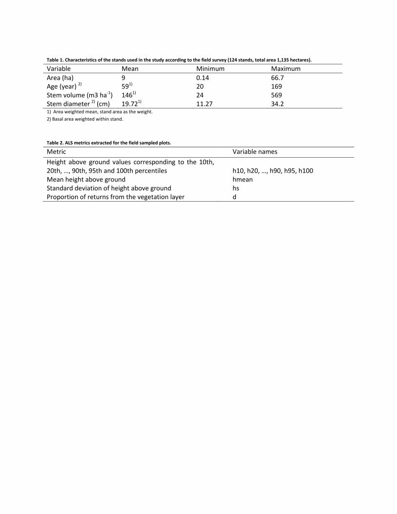
“<Table 1 here>” 156
157
Airborne laser scanning 158
Strömsjöliden was scanned using the ALS system TopEye (S/N 425) carried by a helicopter in the 159
3rd and 5th of August 2008, operated by the contractor Blom Sweden AB. Flying height was 500 160
m above ground and the mission measured approximately 5 pulses per m2. The point data were 161
classified using a progressive Triangular Irregular Network (TIN) algorithm (Axelsson 1999) and 162
(Axelsson 2000) to estimate which returns are measurements of the ground level. Following 163
this, the height above ground was determined for all returns, using a digital elevation model 164
produced from the classified ALS data. A set of fundamental ALS metrics were then computed 165
from the ALS data in accordance to the area based method (Næsset 2002); metrics 166
corresponding to the elevation information, as well as the density of the vegetation, see Table 167
2. A cut-off value of 1.0 m was applied for calculation of metrics. 168
169
“<Table 2 here>” 170
171
Three studied alternatives 172
8
Page 10
R. Saad et al. Scand. J. For. Res., 2014
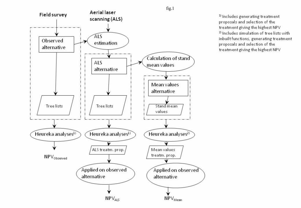
Three alternatives were used in the study. The first alternative was comprised of the field 173
survey observations. The second alternative was based on the ALS metrics. Stand mean values 174
estimated from the second alternative that corresponds to traditional stand register 175
information made up the third alternative, termed later as the mean values alternative, see Fig. 176
1. Tree lists estimated from the ALS alternative and simulated in the DSS in the mean values 177
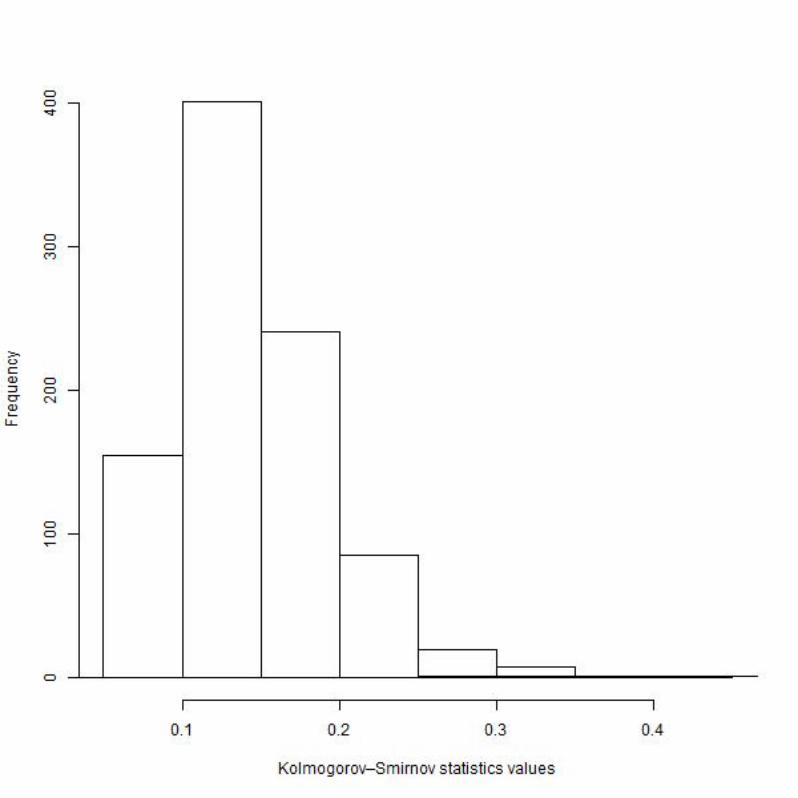
alternative were assumed to have diameter distributions that could be described by a two 178
parameter Weibull function for each plot in the ALS case and per stand in the mean values case. 179
In the ALS case each plot was tested according to Kolmogorov-Smirnoff test to measure the 180
goodness of fit of the estimated Weibull distribution and approximately 96% (869 out of 909) of 181
the null hypothesizes were not rejected, meaning that the diameter distributions are likely to 182
follow the Weibull distribution assumption, see appendix 1. That is, in the ALS alternative the 183
stand level tree list when aggregated over plots did not necessarily follow a Weibull 184
distribution. As the mean values alternative were estimated from the ALS alternative, these two 185
alternatives were in many parts comparable, that is, the study is not aiming at comparison of 186
the accuracy of different forest information acquisition methods. The elaborations of the three 187
data sets are described below, see also Fig. 1. 188
Observed alternative 189
The data acquired in the field survey of the case study area made up the observed alternative. 190
As all trees on sample plots within the stands were callipered tree lists were available. 191
192
ALS alternative 193
9
Page 11
R. Saad et al. Scand. J. For. Res., 2014
Based on the observed alternative and the ALS data functions estimating plot level forest 194
variables including diameter distribution were elaborated. Along with the ALS metrics also the 195
proportion basal area of pine was used as it turned out to be an important variable. This 196
information is typically available in stand registers. 197
198
The diameter distribution of each plot was modeled as a two parameter Weibull distribution 199
using the following steps: 200
1- A Weibull distribution was fitted to the stem diameter measurements for each plot in 201
the observed (field survey) alternative to estimate the two parameters of the 202
distribution, namely scale and shape. 203
2- Multiple linear regression was used, after stepwise regression, to relate the ALS metrics 204
and the proportion of pine from the plot sampling alternative to the scale and shape 205
parameters estimated from the field survey alternative in step 1. In this process the 206
scale and shape were the dependent variables, and the ALS metrics and proportion of 207
pine were the independent variables. 208
3- Scale and shape parameter estimates were predicted for each plot using the regression 209
estimation for the ALS independent variables and the proportion of pine estimated from 210
step 2. 211
212
Expected diameter (ALS estimation) of each plot was compared with the mean diameter of the 213
sample field survey of each plot in order to validate the estimation. Expected diameter, E(D), 214
of the fitted two parameters Weibull distribution was computed as follows: D describe the 215
10
Page 12
R. Saad et al. Scand. J. For. Res., 2014
diameter and it is a Weibull distributed (Hogg & Tanis 2010, page 170) random variable 216
D~Weibull(λ, κ), where λ and κ are the two parameter of Weibull distribution. Expected value 217
of D is given by Equation (1): 218
(1) 𝐸𝐸(𝐷𝐷) = 𝜆𝜆 ∙ Γ �1 + 1𝜅𝜅�, 219
where λ is the distribution scale, κ is the distribution shape and Γ is the gamma function 220
Γ(z) = (z − 1)!, where z is a integer and the sign ! is factorial. 221
222
Values for the basal area per hectare, the number of stems per hectare, the basal area 223
weighted mean height and the quadratic mean diameter were estimated using the ALS 224
independent variables and the proportion pine from the observed alternative, in the same way 225
as the scale and shape were estimated in step 3. In order to estimate these variables linear 226
regression was employed (after applying the stepwise regression) where the dependent 227
variables were the variables in the observed alternative and the independent variables were 228
the ALS independent variables and the proportion pine. The variables mentioned above were 229
predicted for each plot using the regression estimates for the ALS independent variables and 230
the proportion pine as it was done for scale and shape in step 3. Tree species proportions per 231
plot and site variables from the observed alternative were used when the different alternatives 232
were imported to the Heureka DSS. 233
234
An essential step in the processing of the ALS data was the generation of tree lists. This was 235
achieved by using the fitted Weibull distribution parameters to generate a diameter 236
distribution for each plot, incorporating the fitted number of stems per hectare (estimated for 237
11
Page 13
R. Saad et al. Scand. J. For. Res., 2014
each plot separately). One diameter value was assigned to each 10th percentile of the diameter 238
distribution. Each percentile represented a diameter class boundary. First the basal areas 239
corresponding to the upper and lower diameter class boundary were calculated. The diameter 240
corresponding to the mean of the upper and lower basal area was then the diameter 241
representing the diameter class. Each diameter that representing the diameter class, was 242
replicated by the number of trees of each diameter class. The sum of trees over the diameter 243
classes then made up the total number of trees on the plot. 244
245
Mean values alternative 246
The mean values alternative (corresponding to stand register mean values) of each stand was 247
simply averaged from the ALS alternative. That is, the mean value alternative was derived from 248
the ALS alternative and not the observed alternative. 249
250
“<Figure 1 here>” 251
252
Software used for calculations and handling of the different alternatives 253
The R Program, the free software programming language and a software environment for 254
statistical computing and graphics, was used for calculations (regression analysis etc.) and 255
handling of the three alternatives. 256
257
Accuracy measurement 258
12
Page 14
R. Saad et al. Scand. J. For. Res., 2014
To assess the accuracy of the estimated diameter distributions, the tree lists for each plot were 259
first scaled, using the plot area, to obtain the number of trees per hectare in each stand 260
separately. This was done for all three alternatives, and subsequently the estimated diameter 261
distribution accuracy was determined using two error indices, computed for each stand 262
separately using the diameter classes’ absolute differences. 263
264
The first error index (e, Equation 2) gives one measure of the degree of the diameter 265
distribution errors, in which the total number of the trees is taken into account. Its value can 266
range between 0 to 200, where 0 represents a perfect match between two compared 267
distributions. 268
(2) 𝑒𝑒 = ∑ 𝑒𝑒𝑗𝑗15𝑗𝑗=1 = 100 ∙ ∑
�𝑛𝑛𝑜𝑜𝑜𝑜−𝑛𝑛𝑝𝑝𝑜𝑜�𝑁𝑁
15𝑗𝑗=1 , 269
Here, ej is the error in diameter class j (of 15 classes from 0 to 30 cm with 2 cm increments), 270
noj is the number of observed trees in diameter class j and npj is the number of predicted trees 271
in diameter class j, N is the observed total number of trees. The stand level error is the sum of 272
the diameter class errors ej. This error index, which was first proposed by Reynolds et al. 273
(1988), has been widely used in previous studies, e.g. Gobakken & Næsset (2004) and 274
Gobakken & Næsset (2005). 275
276
The second error index (δ, Equation 3), termed the total variation distance index (Levin et al. 277
2009), measures a degree of the diameter distribution errors that is independent of the total 278
number of trees. Each diameter class in each stand was divided by the total number of stand 279
13
Page 15
R. Saad et al. Scand. J. For. Res., 2014
trees in order to obtain a diameter probability distribution. The value of index δ can range 280
between 0 to 1, where 0 represents a perfect match of two compared distributions. 281
(3) 𝛿𝛿 = ∑ 𝛿𝛿𝑗𝑗15𝑗𝑗=1 = 1
2∙ ∑ �𝑃𝑃�𝑥𝑥𝑗𝑗� − 𝑄𝑄�𝑥𝑥𝑗𝑗��15
𝑗𝑗=1 , 282
where δj is the error in diameter class j, P�xj� is the observed relative frequency of diameter 283
class j, and Q�xj� is the relative frequency of diameter class j in the diameter distribution 284
predicted by either the ALS or mean values alternatives. The error index is multiplied by ½ to 285
scale the error between 0 and 1. P�xj� is calculated by dividing the observed number of trees in 286
each class by the observed total number of trees in the stand. Q�xj� is calculated by dividing 287
the number of predicted trees in each class by the predicted total number of trees in the stand. 288
The stand level error is the sum of the diameter class errors δj. 289
290
Calculation of suboptimal losses 291
Each of the three alternatives was imported into the Heureka system (see Fig. 1). The observed 292
alternative and ALS alternative were imported as tree lists, while Heureka simulated tree lists in 293
the mean value alternative. This was done using functions implemented in the software that 294
estimate the scale and shape of stands by taking into account tree species, mean stand age, 295
tree age uniformity and quadratic mean diameter. The Heureka system simulates tree list in a 296
similar way as the simulation tree list was done for the ALS alternative with two main 297
differences. The first difference is that Heureka uses stand level estimated scale and shape 298
where in the ALS alternative the estimated and fitted scale and shape were used (changed from 299
plot to plot). The second notable difference is that Heureka takes equal diameter class intervals 300
14
Page 16
R. Saad et al. Scand. J. For. Res., 2014
containing different tree numbers, while the ALS simulation uses unequal diameter classes 301
containing equal numbers of trees. 302
303
In Heureka, a set of potential management alternatives is generated. A management 304
alternative is a sequence over time of management actions such as regeneration, thinning and 305
final felling. Each action has a calculated net cost or income, and a NPV is calculated for each 306
potential management alternative. Then for each stand the alternative providing the highest 307
NPV is selected. The optimal management strategies selected for the ALS and mean values 308
alternatives were then applied to the forest information in the observed alternative. The 309
differences between the NPV of the observed alternative to the NPV of the applied programs 310
on the forest information in the observed alternative were considered to be the suboptimal 311
losses. The applied treatment programs were fixed only for the two first periods (10 years) 312
since it is expected that in the future new and better information is probable after a period of 313
time (Holmström et al. 2003). The aim was to determine if losses from suboptimal decision can 314
be decreased by using ALS estimations rather than the mean values alternative which is 315
traditionally used in forest planning. 316
317
Results 318
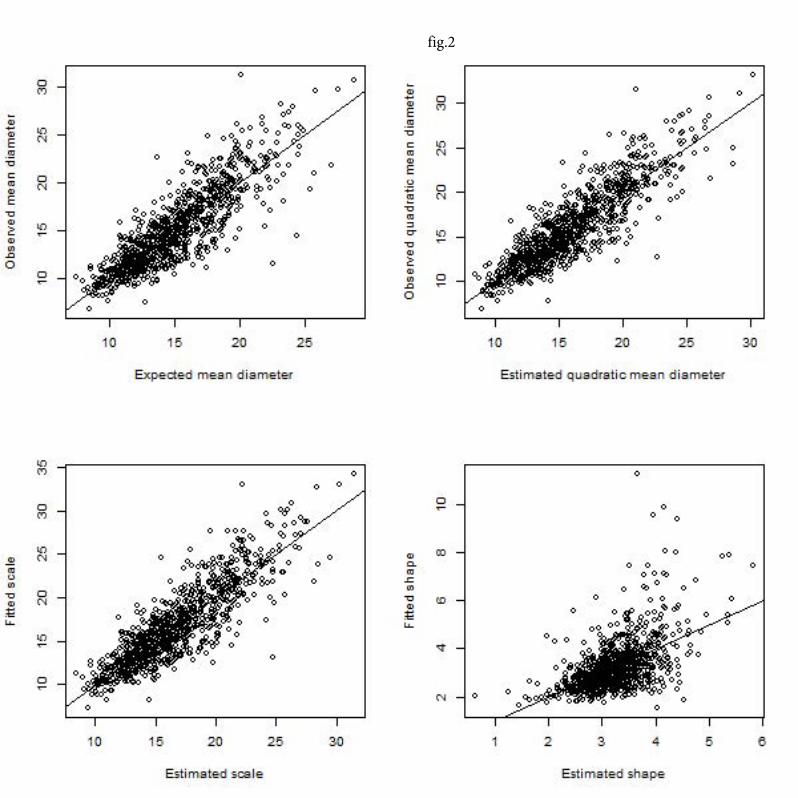
The estimated scale and shape in the ALS alternative were used to estimate the expected 319
diameter of trees in each plot. This was then compared with the mean diameters obtained from 320
the field survey data to validate the ALS estimation. Figure 2 shows mean diameters and 321
quadratic mean diameters from the survey data compared to the expected values estimated in 322
15
Page 17
R. Saad et al. Scand. J. For. Res., 2014
the ALS alternative (Equation 1). Figure 2 also shows the Weibull distribution scale and shape 323
parameters compared to the estimated values in the ALS alternative. 324
325
“<Figure 2 here>” 326
327
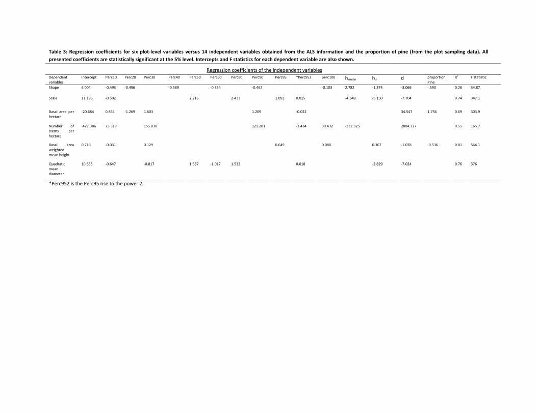
The regression results for six dependent forest variables, with 15 independent variables, are 328
summarized in Table 3. The independent variables are the ALS variables as described in the 329
Methods section and the proportion of pine from the plot sampling alternative. The 330
independent variable Percentile70 was not included since it was found to have insignificant 331
effects (at a significant level of 5%) on the dependent variables. 332
333
“<Table 3 here> 334
335
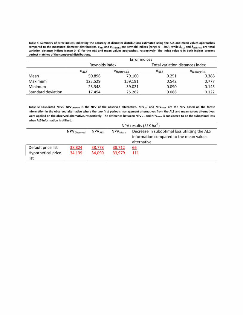
Calculated error indices, indicating the closeness of the estimated diameter distributions to the 336
measured stand level diameter distributions, are summarized in Table 4. 337
338
“<Table 4 here>” 339
340
Table 4 shows that the ALS information yields smaller error indices than the mean values. 341
342
16
Page 18
R. Saad et al. Scand. J. For. Res., 2014
NPV results 343
The NPV calculated in the three alternatives and the suboptimal losses are presented in Table 5. 344
Two different price lists were used for sensitivity analysis. 345
346
“<Table 5 here>” 347
348
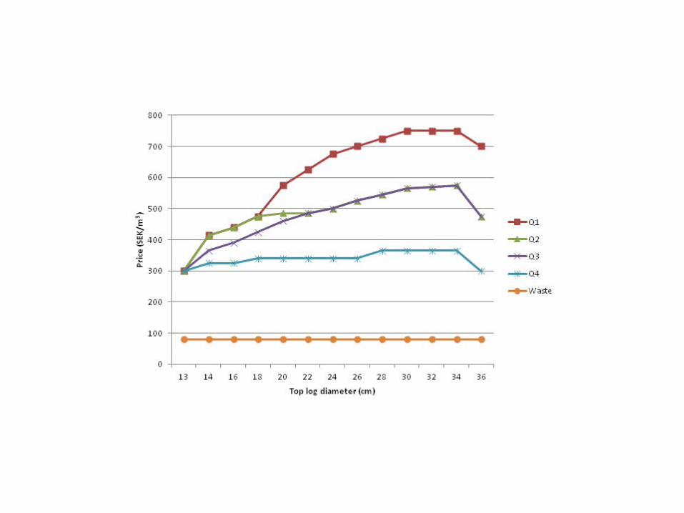
NPVs were calculated using a 3% real interest rate and two different price lists. The effects of 349
interest rate (3% vs 10%) and the growth model used (a stand growth model vs individual tree 350
growth model (Fahlvik et al. 2014)) were also checked but were found to have little impact on 351
suboptimal losses. The default price list used by Heureka, based on pulpwood and sawn timber 352
pricings in mid-Sweden for 2013 (see Appendix 1), resulted in small suboptimal losses (see 353
Table 5). However, as can be seen in Appendix 1, this default price list is not very sensitive to 354
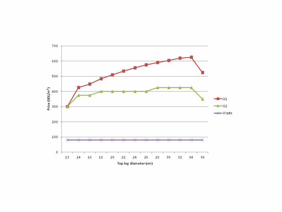
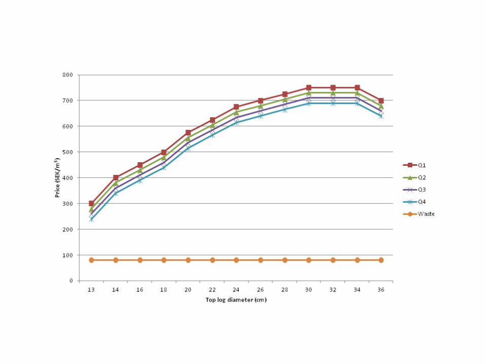
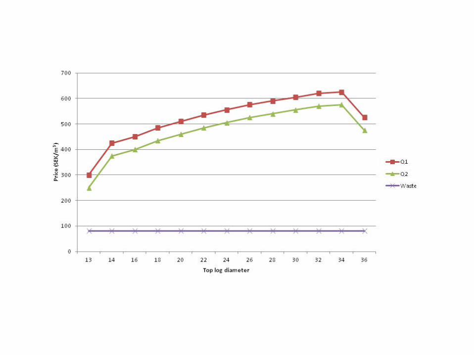
log diameters. This necessitated the construction of a hypothetical price list in which sawn 355
timber prices increased with log diameter, following the curve for the highest log quality, and 356
pulpwood prices were decreased by 50 percent of the mid-Sweden prices for 2013 (see 357
Appendix 1). Use of this hypothetical pricelist increased the estimated difference in suboptimal 358
losses, the ALS alternative yielding 111 SEK ha-1 smaller suboptimal losses than the mean value 359
alternative (Table 5). 360
361
Discussion 362
17
Page 19
R. Saad et al. Scand. J. For. Res., 2014
In this study diameter distributions of stems on plots within stands were estimated from ALS 363
information, assuming that they followed Weibull distributions, and the two parameters – scale 364
and shape – of the distribution for each plot were estimated. Stand level tree lists were then 365
simulated based on the plotwise diameter distributions and then imported to the Heureka 366
forest DSS. This approach was compared to an approach were estimated stand mean values 367
only were used and imported to Heureka. In Heureka tree lists were then simulated using 368
inbuilt default Weibull distribution parameters corresponding to a single plot per stand but 369
different parameters for different species. The ALS-derived tree lists yielded smaller suboptimal 370
losses than the lists generated from stand mean values. Thus, in addition to providing robust 371
estimates of stand characteristics such as tree height and basal area, ALS can provide valuable 372
estimates of diameter distributions, thereby improving forest planning. Furthermore the use of 373
error indexes also showed that the stand level ALS based tree lists was closer to the observed 374
diameter distributions than the Heureka derived tree lists. 375
376
The use of ALS information resulted in up to 111 SEK ha-1 smaller suboptimal losses (using the 377
hypothetical price list) than the mean values approach. As ALS information is already available 378
for estimating mean values of stand characteristics, the only additional costs are in estimating 379
the diameter distribution, thus the marginal profit can be increased by a similar amount to the 380
suboptimal loss reduction. These results also reveal that long-term NPV calculations are 381
substantially less sensitive to estimated diameter distributions than other factors such as 382
volume, age, height and site index. However, diameter distributions have potentially greater 383
18
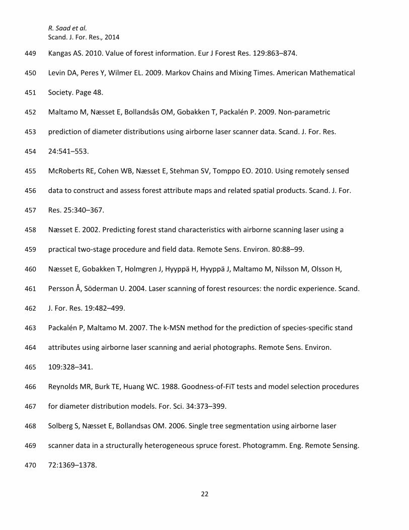
Page 20
R. Saad et al. Scand. J. For. Res., 2014
impacts on short-term NPVs, for instance those related to the dimensional demands of 384
sawmills. 385
386
In most cases the Weibull scale parameter was estimated notably more accurately than the 387
shape parameter. This is to be expected as the area-based ALS approach will provide a low 388
number of measurements for individual trees. It provides accurate information on the height 389
and density of trees, but is less able to distinguish whether a forest consists of numerous thin 390
trees, or fewer thicker trees. Estimates of the shape parameter could also be improved by 391
higher density ALS sampling and use of larger sample plots, which would provide more accurate 392
reference data for the subsequent modeling of diameter distributions. 393
394
In the regression modeling of diameter distribution parameters from ALS information the 395
proportion of pine trees in each plot was used as an independent variable as well as height 396
percentiles. The proportion of pine trees was needed as the relationship between diameter 397
distributions and ALS data is different for different tree species. In this study, the diameter 398
distribution of all species in each plot was modeled; in order to take the species variations into 399
account the proportion of tree pine was included as an independent variable. In operational 400
practice, this information cannot be estimated directly from ALS information but can be 401
acquired by aerial photo interpretation and potentially also by computerized algorithms using 402
aerial laser scanning data and digital aerial photos (Packalén & Maltamo 2007). A proxy for plot 403
level pine proportion is also readily available in existing stand registers. 404
405
19
Page 21
R. Saad et al. Scand. J. For. Res., 2014
A potential way to further improve the approach is to use non-parametric methods to estimate 406
plot level diameter distributions, as described by Gobakken (2005) and Maltamo et al. (2009). In 407
such a case no parametric diameter distribution is assumed (in contrast to our assumption of 408
Weibull distributions), and in operational applications today imputation techniques, based for 409
instance on kMSN methods (Maltamo et al. 2009), are usually applied. In this approach, 410
predictions are made using the actual diameter measurements in the reference data and no 411
smoothing or distribution assumptions are needed. Such methods can be further evaluated in 412
future studies to assess their potential for improving data to be used in forest DSSs. 413
414
In conclusion, the results of the study indicate that ALS-based estimates of diameter 415
distributions have the potential to further improve the planning process, although in this study 416
the gain in NPV was not very high. Use of ALS data should reduce losses from suboptimal 417
decisions, but the level of reduction depends on, e.g., the design of timber price list. 418
419
420
References 421
422
Axelsson P. 1999. Processing of laser scanner data—algorithms and applications. ISPRS Journal 423
of Photogrammetry & Remote Sensing. 54:138–147. 424
Axelsson P. 2000. DEM generation from laser scanner data using adaptive TIN models. 425
International Archives of Photogrammetry and Remote Sensing. 33:110–117. 426
20
Page 22
R. Saad et al. Scand. J. For. Res., 2014
Borges JG, Nordström E.M., Garcia-Gonzalo J, Hujala T., Trasobares A (Eds.). 2014. Computer-427
based tools for supporting forest management. The experience and the expertise world-wide. 428
Umeå (Sweden): Swedish University of Agricultural Sciences, Department of Forest Resource 429
Management. 430
Breidenbach J, Næsset E, Lien V, Gobakken T, Solberg S. 2010. Prediction of species specific 431
forest inventory attributes using a nonparametric semi-individual tree crown approach based 432
on fused airborne laser scanning and multispectral data. Remote Sens. Environ. 114:911–924. 433
Duvemo K, Lämås T. 2006. The influence of forest data quality on planning processes in 434
forestry. Scand. J. For. Res. 21:327–339. 435
Fahlvik N, Wikström P, Elfving B. 2014. Evaluation of growth models used in the Swedish Forest 436
Planning System Heureka. Silva Fennica. 48:2. 437
Gobakken T, Næsset E. 2004. Estimation of diameter and basal area distributions in coniferous 438
forest by means of airborne laser scanner data. Scand. J. For. Res. 19:529–542. 439
Gobakken T, Næsset E. 2005. Weibull and percentile models for lidar-based estimation of basal 440
area distribution. Scand. J. For. Res. 20:490–502. 441
Gordon SN, Floris A, Boerboom L, Lämås T, Eriksson LO, Nieuwenhuis M, Garcia J, Rodriguez L. 442
2013. Studying the use of forest management decision support systems: An initial synthesis of 443
lessons learned from case studies compiled using a semantic wiki. Scand. J. For. Res. 444
DOI:10.1080/02827581.2013.856463. 445
Hogg RV, Tanis EA. 2010. Probability and Statistical Inference. New Jersey: Pearson. 446
Holmström H, Kallur H, Ståhl G. 2003. Cost-plus-loss analyses of forest inventory strategies 447
based on kNN assigned reference sample plot data. Silva Fennica. 37:381–398. 448
21
Page 23
R. Saad et al. Scand. J. For. Res., 2014
Kangas AS. 2010. Value of forest information. Eur J Forest Res. 129:863–874. 449
Levin DA, Peres Y, Wilmer EL. 2009. Markov Chains and Mixing Times. American Mathematical 450
Society. Page 48. 451
Maltamo M, Næsset E, Bollandsås OM, Gobakken T, Packalén P. 2009. Non-parametric 452
prediction of diameter distributions using airborne laser scanner data. Scand. J. For. Res. 453
24:541–553. 454
McRoberts RE, Cohen WB, Næsset E, Stehman SV, Tomppo EO. 2010. Using remotely sensed 455
data to construct and assess forest attribute maps and related spatial products. Scand. J. For. 456
Res. 25:340–367. 457
Næsset E. 2002. Predicting forest stand characteristics with airborne scanning laser using a 458
practical two-stage procedure and field data. Remote Sens. Environ. 80:88–99. 459
Næsset E, Gobakken T, Holmgren J, Hyyppä H, Hyyppä J, Maltamo M, Nilsson M, Olsson H, 460
Persson Å, Söderman U. 2004. Laser scanning of forest resources: the nordic experience. Scand. 461
J. For. Res. 19:482–499. 462
Packalén P, Maltamo M. 2007. The k-MSN method for the prediction of species-specific stand 463
attributes using airborne laser scanning and aerial photographs. Remote Sens. Environ. 464
109:328–341. 465
Reynolds MR, Burk TE, Huang WC. 1988. Goodness-of-FiT tests and model selection procedures 466
for diameter distribution models. For. Sci. 34:373–399. 467
Solberg S, Næsset E, Bollandsas OM. 2006. Single tree segmentation using airborne laser 468
scanner data in a structurally heterogeneous spruce forest. Photogramm. Eng. Remote Sensing. 469
72:1369–1378. 470
22
Page 24
R. Saad et al. Scand. J. For. Res., 2014
Wikström P, Edenius L, Elfving B, Eriksson LO, Lämås T, Sonesson J, Öhman K, Wallerman J, 471
Waller C, Klintebäck F. 2011. The Heureka forestry decision support system: an overview. 472
Mathematical and Computational Forestry&Natural-Resource Sciences. 3:87–94. 473
474
Appendix 1. 475
“<Figure 1 pine default prices here>” 476
“<Figure 2 spruce default prices here>” 477
“<Figure 3 pine hypothetical prices here>” 478
“<Figure 4 spruce hypothetical prices here>” 479
“<Figure 5 histogram of Kolmogorov-Smirnoff statistics values here >” 480
23
Page 27
Table 1. Characteristics of the stands used in the study according to the field survey (124 stands, total area 1,135 hectares).
Variable Mean Minimum Maximum Area (ha) 9 0.14 66.7 Age (year) 2) 591) 20 169 Stem volume (m3 ha-1) 1461) 24 569 Stem diameter 2) (cm) 19.721) 11.27 34.2 1) Area weighted mean, stand area as the weight. 2) Basal area weighted within stand.
Table 2. ALS metrics extracted for the field sampled plots.
Metric Variable names Height above ground values corresponding to the 10th, 20th, …, 90th, 95th and 100th percentiles h10, h20, …, h90, h95, h100 Mean height above ground hmean Standard deviation of height above ground hs Proportion of returns from the vegetation layer d
Page 28
Table 3: Regression coefficients for six plot-level variables versus 14 independent variables obtained from the ALS information and the proportion of pine (from the plot sampling data). All presented coefficients are statistically significant at the 5% level. Intercepts and F statistics for each dependent variable are also shown.
Regression coefficients of the independent variables Dependent variables
Intercept Perc10 Perc20 Perc30 Perc40 Perc50 Perc60 Perc80 Perc90 Perc95 *Perc952 perc100 hmean hs d proportionPine
R2 F statistic
Shape 6.004 -0.493 -0.496 -0.589 -0.354 -0.462 -0.103 2.782 -1.374 -3.066 -.593 0.26 34.87
Scale 11.195 -0.502 2.216 2.433 1.093 0.015 -4.348 -5.150 -7.704 0.74 347.1
Basal area per hectare
-20.684 0.854 -1.269 1.603 1.209 -0.022 34.547 1.756 0.69 303.9
Number of stems per hectare
-427.386 73.319 155.038 121.281 -3.434 30.432 -332.325 2804.327 0.55 165.7
Basal area weighted mean height
0.716 -0.031 0.129 0.649 0.088 0.367 -1.078 -0.536 0.81 564.1
Quadratic mean diameter
10.635 -0.647 -0.817 1.687 -1.017 1.532 0.018 -2.829 -7.024 0.76 376
*Perc952 is the Perc95 rise to the power 2.
Page 29
Table 4: Summary of error indices indicating the accuracy of diameter distributions estimated using the ALS and mean values approaches compared to the measured diameter distributions. 𝐞𝐞𝐀𝐀𝐀𝐀𝐀𝐀 and 𝐞𝐞𝐇𝐇𝐞𝐞𝐇𝐇𝐇𝐇𝐞𝐞𝐇𝐇𝐇𝐇 are Reynold indices (range 0 – 200), while 𝛅𝛅𝐀𝐀𝐀𝐀𝐀𝐀 and 𝛅𝛅𝐇𝐇𝐞𝐞𝐇𝐇𝐇𝐇𝐞𝐞𝐇𝐇𝐇𝐇 are total variation distance indices (range 0 -1) for the ALS and mean values approaches, respectively. The index value 0 in both indices present perfect matches of the compared distributions. Error indices Reynolds index Total variation distances index 𝑒𝑒𝐴𝐴𝐴𝐴𝐴𝐴 𝑒𝑒𝐻𝐻𝐻𝐻𝐻𝐻𝐻𝐻𝐻𝐻𝐻𝐻𝐻𝐻 𝛿𝛿𝐴𝐴𝐴𝐴𝐴𝐴 𝛿𝛿𝐻𝐻𝐻𝐻𝐻𝐻𝐻𝐻𝐻𝐻𝐻𝐻𝐻𝐻 Mean 50.896 79.160 0.251 0.388 Maximum 123.529 159.191 0.542 0.777 Minimum 23.348 39.021 0.090 0.145 Standard deviation 17.454 25.262 0.088 0.122
Table 5: Calculated NPVs. NPVObserved is the NPV of the observed alternative. NPVALS and NPVMean are the NPV based on the forest information in the observed alternative where the two first period’s management alternatives from the ALS and mean values alternatives were applied on the observed alternative, respectively. The difference between NPVALS and NPVMean is considered to be the suboptimal loss when ALS information is utilized.
NPV results (SEK ha-1) NPVObserved NPVALS NPVMean Decrease in suboptimal loss utilizing the ALS
information compared to the mean values alternative
Default price list 38,824 38,778 38,712 66 Hypothetical price list
34,139
34,090
33,979 111