Scientific Challenges Associated with Sea Ice-Drift … · Scientific Challenges Associated with...

Envisat Summer School 16-26 Aug, 2004 M.R. Drinkwater - 18-Aug-04

Scientific Challenges Associated with Sea Ice-Drift Products

Mark R. DrinkwaterEuropean Space Agency-ESTEC

Oceans/Ice Unit, Science & Applications Dept.Earth Observation Programmes Directorate


Contents

• Introduction– What is sea ice and how does it form?– Why is ice drift important?– What time and space scales are important?

• Goals and Challenges of Ice Drift Measurement• Characteristics of Sea Ice Drift• Methods of Ice Drift Measurement

– Buoys– Satellite Data– Validation of Ice Drift Velocities– Optimally Interpolated/Blended Products

• From Ice Drift to Volume Fluxes• Remaining Challenges

– Sub-daily ice motion– Assimilating velocity data


What is sea-ice?

– Sea ice forms on the surface of the polar oceans when seawater freezes (see: http://oceans-www.jpl.nasa.gov/polar/SeaIce.html or

http://www.antcrc.utas.edu.au/aspect/seaiceglossary.html)

– A large temperature difference between polar ocean and atmosphere, coupled with strong winds results in vigorous turbulent fluxes of sensible and latent heat. The consequence of the extraction of heat from the upper water column is the growth of a sea-ice layer

– Sea-ice is an effective insulator and a reflector. The extent and fraction (concentration) of the ocean surface covered by sea-ice regulates the amount of incoming shortwave energy, and the net energy loss to the atmosphere.

– The representation of sea-ice in models has traditionally been crude, and the critical impact of sea-ice on the global system until recently had been underestimated.


Sea ice formation

Calm Conditions Rough Conditions

Grease ice

Nilas ice

Grey ice

Pancake ice

ConsolidateConsolidatedpancakesdpancakes

Compression/ Compression/ DeformationDeformation Ridged ice

Aging


What is ice motion or ice drift?

– Ice drift occurs by the transfer of momentum from the atmosphere to the sea-ice (wind stress a function of V2

wind and atmosphere-ice drag)– Ice drift also transfers momentum to the upper ocean – Net impact of ice drift is to carry ice equatorward to melt.– The concentration, extent and drift of sea-ice as such regulates the energy

balance of the polar regions

Why is ice drift important ?

– Ice motion is the movement of individual ice floes or larger contiguous units comprising groups of individual floes

– Velocity of ice motion is determined by accurately measuring the position of an ice floe at times t1 and t2and distance travelled over the interval ∆t (t2-t1)


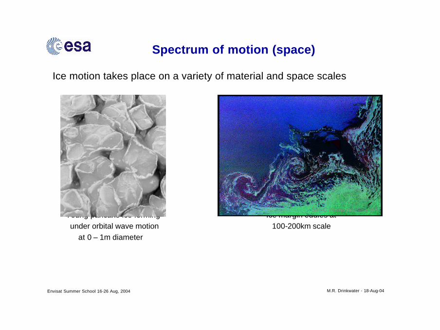
Spectrum of motion (space)

Ice motion takes place on a variety of material and space scales

Young pancake ice forming Ice margin eddies atunder orbital wave motion 100-200km scale

at 0 – 1m diameter

SIR-C image courtesy JPL


semi-diurnal tides

diurnal tides

storms

Spectrum of motion (time)

Periodograms of u and v components (cm/s) of ice velocity for Ice Station Weddell, for days 50-76,1992.


Goals & Challenges

• The principal goal is to quantify sea-ice velocity globally (i.e. Arctic and Antarctic) on appropriate scales (i.e. f > 1 d-1 and res. < 10 x 10 km) with which to characterise ice drift patterns

• The secondary goal is to validate the ice drift estimates using independent data and to deliver seasonally evolving error statistics to facilitate model-data assimilation

• The challenges are to:– deliver global, continuous (i.e. year-round) high-frequency, high

spatial resolution ice motion products– minimise the effects of atmospheric disturbances– optimally blend different sources of ice drift (satellite + buoy)– quantify the effects of tidal/inertial motion on sub-daily timescales– provide data that can be assimilated into models


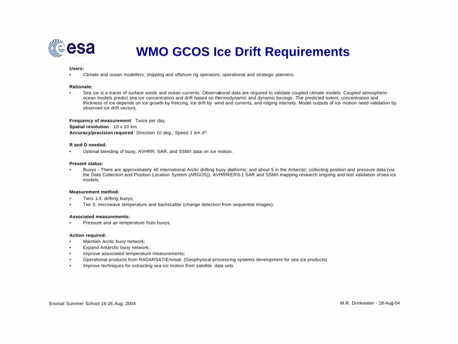
WMO GCOS Ice Drift RequirementsUsers:• Climate and ocean modellers; shipping and offshore rig operators; operational and strategic planners.

Rationale:• Sea ice is a tracer of surface winds and ocean currents. Observational data are required to validate coupled climate models. Coupled atmosphere-

ocean models predict sea ice concentration and drift based on thermodynamic and dynamic forcings . The predicted extent, concentration and thickness of ice depends on ice growth by freezing, ice drift by wind and currents, and ridging intensity. Model outputs of ice motion need validation by observed ice drift vectors.

Frequency of measurement: Twice per day. Spatial resolution : 10 x 10 km. Accuracy/precision required : Direction 10 deg.; Speed 1 km d-1.

R and D needed:• Optimal blending of buoy, AVHRR, SAR, and SSM/I data on ice motion.

Present status:• Buoys - There are approximately 40 international Arctic drifting buoy platforms; and about 5 in the Antarctic; collecting position and pressure data (via

the Data Collection and Position Location System (ARGOS)). AVHRR/ERS-1 SAR and SSM/I mapping research ongoing and test validation of sea ice models.

Measurement method:• Tiers 1-3: drifting buoys;• Tier 5: microwave temperature and backscatter (change detection from sequential images).

Associated measurements:• Pressure and air temperature from buoys.

Action required: • Maintain Arctic buoy network;• Expand Antarctic buoy network;• Improve associated temperature measurements;• Operational products from RADARSAT/Envisat. (Geophysical process ing systems development for sea ice products) • Improve techniques for extracting sea ice motion from satellite data sets


Characteristics of Sea-Ice Drift


So how does sea-ice drift?

• Buoys deployed around Ice Station Weddell – 1 (ISW-1) in 1992

• Buoys indicate bouts of uniform drift, separated by aperiodic loops and meanders

• Resulting drift is a balance between wind and current and internal ice stresses, and Coriolis force

• Buoys in central pack – away from coast – exhibit relatively free drift

• Buoys in vicinity of coast exhibit the effects of internal stresses (i.e. floe-floe) transferred through the ice pack


Drift of Ice Station Weddell

10 m air temp

10 m wind vector

ISW drift vector

25 m depth current

after Geiger and Drinkwater, In Press


Fracture of ice cover

• 1992 Example of 20 x 20 km box near ISW-1 in ERS-1 SAR image pair separated by 6 day interval.

• Lead appearance indicates divergence and fracture of the ice cover

• Ice motion is discontinuous, with large areas of uniform velocity, separated by areas of strong velocity gradients (shear zones).

• Non-uniform ice motion fractures the ice, exposing the ocean surface to the atmosphere



Ice Drift simplified

• An approximation for free-drift is that the time-mean ice velocity ( ) is in balance with the geostrophic wind and the mean current (assuming internal ice stress is negligible):

- where matrix A comprises a scale factor |A| and turning angle δ (between the wind and ice vector)

• It follows that the time-varying part of the motion responds to the time-varying part of the wind:

- where is zero. e contains all errors, including any internal ice stress gradient or time-dependence of the current (e.g. tides).

currentice vGAv +=

icevG

eGAvice +′=′

currentv

e


See:

2 WWGS ’92 buoy + SAR drift slides

& Arctic ERS SAR example


SLP + Ice Drift + Ice Concentration

after Venegas et al., 2001

• SVD analysis of 20 year SSMI drift data set (using Multi-taper method)• Spatial reconstruction of the dominant 4-year cycle component (ENSO-forced) • Anomalies of Ice drift , sea-ice-concentration & SLP are in phase• Sea-ice drift sustains positive anomalies


Methods of Ice Drift Measurement


Traditional methods of ice-driftvelocity determination

• Buoys/Drift Camps (Argos and GPS positioning)– Around 10 positions per day– ARGOS ~0.3 km positional accuracy (Doppler shift)– GPS ~100 m accuracy

• Success dependent upon ice deformation; battery lifetime; upright transmitter– At right: one of an array of 5 AWI buoys (#9369) deployed on

deformed ThFY ice during WWGS’92 by helicopter– Buoy 9369 half circumnavigated

Antarctica in 1992-1993

Photo courtesy M. Drinkwater


WCRP International Arctic Buoy Program (IABP)

• Several buoys deployed per year (limited by air-drop logistics): Argos + GPS

• In contrast to Antarctic, buoys are captive in sea-ice for several years


WCRP International Program for Antarctic Buoys (IBAP) (’89 – ’99)

• Serious limitation of logistics & cost on deployment locations

• Antarctic drifter lifetime severely limited in largely seasonal ice pack

• longest duration on-ice survival of ~2 yrs in Weddell Sea perennial ice pack

• ECMWF and NCEP Sea-level pressure (SLP) analyses seriously degraded in Southern Ocean due to lack of Argos buoys reporting SLP

• Serious lack of in-situ observations in Amundsen-Bellingshausen Seas, where greatest coupled atmosphere-ice-ocean covariability is observed

• Satellites provide exclusive source of ice drift in South-Pacific sector of Southern Ocean


Mean Arctic basin circulation & Isochrones (yrs)

Beaufort

Gyre

Transpolar

Drift


Buoy-derived optimally-interpolated products


• Synthetic Aperture Radar (SAR) [1991 - present day]– loc. accuracy: ~100 m – SeaSat; ERS-1; ERS-2; RadarSat-

1; ENVISAT; – New SARs: ALOS; RadarSat-2; ESA EarthWatch (GMES)

Sentinel 1

• AVHRR (1 km res. 2600 km swath)– limited by illumination/cloud cover

• Passive Microwave Radiometer [1978 - present day]– loc. accuracy: 12.5/25 km - SMMR; SSM/I; AMSR-E

• Scatterometer [1992 - present day]– loc. accuracy: ~10 km - ERS; ~5 km NSCAT; QSCAT – Future operational system ASCAT on METOP-1,2,3

Satellite Datasets for Ice Drift


History of Satellite ice-drift tracking• Originally manual ice floe tracking developed at JPL in early 1980’s using

optically processed Seasat images (~25 m res.) see slide 4• Feature tracking first applied to digitally processed, geolocated Seasat data in

mid ’80s see slide 5• New techniques developed using 1 km AVHRR in late 80’s

– e.g. Maximum cross-correlation (see following slide)• Cross-correlation, wavelet and optical flow tracking now facilitate ice floe drift

measurements at much degraded resolutions, and over broader swath – thus improving frequency of products

• Highlights:– We needed to zoom in to very high res. (10-100m) to push tracking

technology– High-res. High bit-rate SAR floe tracking was only available in direct downlink

receiving station mask regions (see plot of stations in Arctic and Antarctic SAR receiving stations). NRT availability of drift required computer automated procedures & “at-source” processing

– Recent need to zoom out to develop 25 year drift climatology using low-res., broad swath Microwave Radiometer image time series


Deriving Ice Drift

• Pattern recognition techniques first developed using high resolution digital satellite images (e.g. feature recognition – see slide)– Cross-correlation helped to automate ice drift tracking– Cross-correlation (R ) of brightness values between image pair (a and

b) separated at an interval of time yields ice displacement, and velocity over that interval:

• Search performed on small regions (n x n) in images• Maximum cross correlation reveals destination of original feature

∑ ∑+

−=

+

−=

−++−++=

t

tp

t

tqban

bqlpkbaqjpialkjiR

σσ2

)),()(),((),;,(

2/)1( −= nt a aσwhere and and are the mean and std. dev

of ija over the n x n sub-array


Automating Ice Drift Tracking

• Automation of computer drift tracking came in late 1980’s at JPL in preparation for ERS-1– Alaska SAR Facility developed to capture US/Canadian Arctic

SAR coverage (see slide 6 of station masks)– McMurdo receiving station developed to capture almost complete

SAR sea-ice coverage in Antarctica (see slide 7)

• Early 1990’s saw development of the Geophysical Processor System(GPS) at JPL– Implemented at the Alaska SAR Facility for routine, automated,

near-real-time processing of Eulerian, fixed-grid ice motion from SAR image pairs

**See viewgraphs on Alaska SAR Facility GPS ice tracking**

– GPS evolved into RGPS in 1996 with Radarsat Wide-swath capability and first basin-scale SAR mapping capability (examples later)


Challenge: Ice drift everywhere/all the time?

• Swath composite images are necessary (e.g. SSMI or Scatt)

OR alternatively

• Optimal blending of different data flavours is needed

Since:

(1) we require pairs of images for tracking;

(2) we do not have multiple SAR’s with orbits optimised for ice drift:


SAR vs. swath composite 3d image drift products10 – 13 April 2004

• ASAR Global Monitoring Mode (400 km swath, ~1km res.)

• Right-looking SAR fills Arctic hole

• Instantaneous drift on 10 km Eulerian grid

SSMI

QuikScat

Polar Hole

Weather effects

Decorrelation:weather, snow,

melting


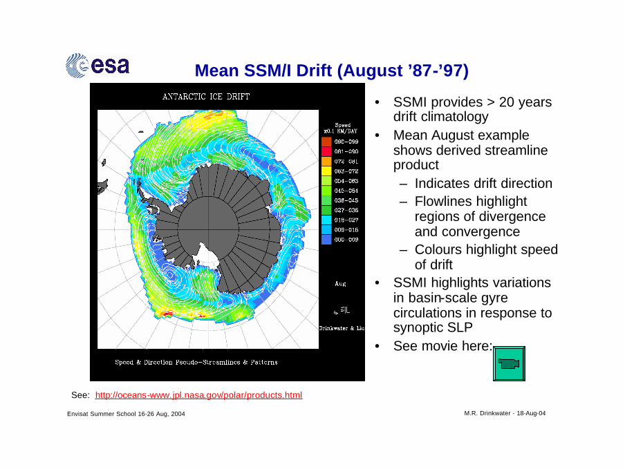
Mean SSM/I Drift (August ’87-’97)

• SSMI provides > 20 years drift climatology

• Mean August example shows derived streamline product– Indicates drift direction– Flowlines highlight

regions of divergence and convergence

– Colours highlight speed of drift

• SSMI highlights variations in basin-scale gyre circulations in response to synoptic SLP

• See movie here:

See: http://oceans-www.jpl.nasa.gov/polar/products.html


Seasonal Variability in Sea-Ice Dynamics

• Seasonally varying dynamics

• Dynamic response to synoptic-scale atmospheric forcing

• Variance in drift speed greatest in central Gyre regions where divergence largest

• Shape and extent of Gyres determined by mean synoptic low pressure over ocean basins

• Off continental shelves:- temporal response < 12hrs- seasonal length scales

• On continental shelves:- temporal response longer- shorter length scales- coastal polynya formation

katabatic winds + tides

Jan-Mar Apr-Jun

Jul - Sep Oct - Nov

See: Drinkwater, M.R., Active Microwave Remote Sensing Observations of Weddell Sea Ice. In Antarctic Research Series , 74, 187-212, American Geophysical Union, 1998


Climatologies: Sea-ice Dynamics

• Assuming tracking uncertainties are uncorrelated - monthly mean drift uncertainties reduced by 1/sqrt(N)

• Differential Kinematic parameters:– Div; Vor; Shear– computed from monthly mean 1 d

motion vector velocity components (u,v)

dydvdxduvdiv ice +=)(r

dydudxdvvvor ice −=)(r

( ) ( )2)( dydudxdvdydvdxduvshear ice ++−=r

Grid cell area change: 3 x 3 cells


Validation of Ice Drift


Validation of Satellite-Derived Ice Drift

• Comparison with ECMWF or NCEP analysis fields

• Comparison with overlapping ARGOS/GPS drifter data – ISW-1 GPS locations vs. SAR-derived drift vectors– WWGS’92 Buoy drifts with SAR drift vectors

• Intercomparisons between various satellite tracked products at differing scales– SAR vs. Scatterometer vs. Passive Microwave Radiometer– Inter-satellite product differences may be used to better

quantify uncertainties due to geolocation, tracking, and swath compositing


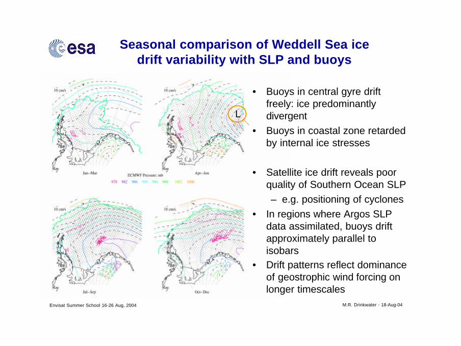
Seasonal comparison of Weddell Sea ice drift variability with SLP and buoys

• Buoys in central gyre drift freely: ice predominantly divergent

• Buoys in coastal zone retarded by internal ice stresses

• Satellite ice drift reveals poor quality of Southern Ocean SLP– e.g. positioning of cyclones

• In regions where Argos SLP data assimilated, buoys drift approximately parallel to isobars

• Drift patterns reflect dominance of geostrophic wind forcing on longer timescales

L


Validation & velocity comparisons with IPAB Buoys

• Examination areas chosen by buoy deployment position and track

• Areas chosen to yield comparisons experiencing different seasonal ice conditions

• North-south coastal regions and east-west coastal regions selected to investigate systematic errors (biases) with respect to satellite orbit

• Coastal regions with shallow/deep water selected to mitigate tidal aliasing


Satellite Drift - rms error distribution • 48 hr running means of buoy velocities used for

comparison with 2d satellite tracking• For each day and buoy, the nearest gridded

satellite drift vectors are interpolated to the buoy location within a fixed search radius using a weighted distance method

– governed by search radii at increasing increments of 200, 400, 600, 800, 1000 km

• Rms errors computed from all satellite-buoy comparisons:

• Scale-dependent global seasonal mean error of 4.58 cm/s (see upper left) for 2 d tracking

– Min. rms error at 200 km length scales in shelf break regions

– Central gyre minimum error at 600km length scale• Bias of –1 cm/s due to orbit sampling pattern and

PMW swath compositing & smearing effects (act as low-pass filter)

• Largest rms errors when compared with eastward propagating buoys in ice margin

– These buoys oppose the orbit propagation direction

2

1

)(1Buoy

Nn

nSatrms vvNe

rr−= ∑

=

=

**Theoretical error (geolocation, tracking and timing error, and swath-

smearing effects) is 4.6 km/d or ~5 cm/s.

Global

rms (cm/s) by region


Optimal Interpolation

• Optimally Interpolated drift (OI) is an advanced analysis product, combining results from different channels (e.g. 37 GHz and the 85 GHz passive microwave radiometer channels) with additional drift information from buoys when geographically and temporally available.

• The data are calculated with the weighting function:

• Weighting coefficients α, β and γdetermined by optimal interpolation.

• Solutions for each point obtained based on the uncertainties, the expected variance of the motion and the distance to available observations

Buoyi

ii

GHzi

ii

GHzi

iiice vvvv ∑+∑+∑= ααα 3785)

White areas signify region of influence of buoys upon sat data OI breaks down as cyclone is directly over Maud Rise on 17 Aug.3 buoys were filtered/rejected from the analysis (in blue coastal vector region). Consequently the interpolationdid not incorporate them and results are poorer


Optimal blending of sparse time-space data with satellite data


Merging SSM/I and Scatterometer Motion

Figure 4. Daily sea-ice motion vector field for December 20, 1996 from (a) 85.5 GHz SSM/I; (b) 13.6 GHz NSCAT;and (c) merged SSM/I and NSCAT data set. Buoy motion vectors are shown in red [after Long and Drinkwater,1999].

• Optimal Blending of datasets provides us with more continuous & contiguous satellite tracking capability

• Allows gaps to be filled

• Challenge remains to track through the summer months when melt ponding occurs


SSM/I Motion + Buoys + NCEP

(a) SSM/I 85 GHz-derived Arctic ice drift from 8-11 April, with IABP buoy drift vectors superimposed. (b) Optimally interpolated (gap-filled) ice drift field

a b


Envisat wide-swath GM mode vs. Scatt + SSMI merged drift

Merged Products from ESA ICEMON Study courtesy R. Ezraty, CERSAT, IFREMER

ftp://ftp.ifremer.fr/ifremer/cersat/products/gridded/psi-drift/quicklooks/arctic/merged/3-daily/2004/


Building up an Arctic-basin-wide ice motion product using high-res. SAR image swath

composites

A case study: RadarSat Geophysical Processorcourtesy R. Kwok - JPL


Arctic Snapshot – using sequential SAR

**See slide for swaths


Lagrangian Grid Strategy

• Coastal grid cells spacing – 25 km

• Central Gyre cell spacing – 10 or 20 km

- depends on computational resources

• Computer tracks ice in each grid cell as long as it can be recognised

• Grid evolves with every time step, in contrast to fixed Eulerian grids

• Lagrangian approach allows each parcel of ice to be followed in time throughout its lifetime (from birth to death)

• Sequential logging of cell area changes allow ridging contribution to thickness redistribution to be quantified


RGPS Lagrangian Tracking


Lagrangian Observationsof Ice Motion and Deformation:

RGPS

101 km 102 km

103 km

3-day sampling


RGPS Example: 3 – 9 Feb, 1998


Sequential Shear Patterns Nov 28 - Dec 28, 1999


Net Divergence (Nov - May, 1997/98)

9.2% net div

Mean motion field and SLP (Nov-May)


Comparison of RGPS Openings with SSM/I Open Water Fraction

0.0

0.5

1.0

1.5

2.0

2.5

3.0

0 20 40 60 80 100 120 140

Day-of-Year 1998

BootstrapNASA TeamRGPS Openings

(Kwok, 2002)

• Generally accepted that there is approximately 2 -4% open water in the interior pack during the winter

**- never validated at the basin scale.

• RGPS Example shows large-scale (spatially and temporally) comparison of the open water estimates from passive microwave retrievals with divergence estimates within the winter ice pack.

– Over the RGPS domain, we find average openings of ~0.3% compared to much larger passive microwave estimates of 2-4%.

– SSMI uncertainty in open water fraction is large and varies depending on the amount of open water

• Assimilation of ice drift kinematic data (and ice concentration) can help correctly specify amount of divergence à open water more accurately

– Assimilation of ice concentration can not improve the state estimates in polar coupled models unless ice concentration accuracy improves (result is too rapid ice growth in winter; and too much melting in summer)


SUMMARY (1)

• Various satellite datasets facilitate daily Eulerian global ice-drift tracking à RGPS now provides Lagrangian drift (1996-97 onwards)

• SAR is most precise/accurate for ice velocity - but limited by the revisit cycle (*all satellites have different revisit times and pseudo sub-cycles)

– limitations are swath-width and daily coverage – integrates drift over 3d or ~1d revisit period– promise for new Global Monitoring Mode of Envisat – using periodic mosaics

• Passive Microwave critical for obtaining >20 yrs ice drift– 1d ice motion relatively low accuracy (rms=5.6 km/d) --> 2 or 3 day drift more

accurate– ideal for monthly and annual climatologies, and study of drift impact on ice extent

• Swath Composite Products from Passive Microwave/Scatterometer– NSCAT/QSCAT is a limited dataset: ERS (1992 - present)– aliasing effects in swath composites need to be modelled

• Challenge of sea-ice drift “everywhere all the time” is now being met – but with relatively large residual uncertainties in ice velocity– Optimal interpolated products to some extent remedy this situation– Seasonally-, and spatially error covariance statistics must be derived– Ideally daily, global SAR ice drift is needed


Application Case Study:

From Ice Drift to Ice Fluxes


Arctic Ice Export vs. NAO

• Ice drift across the Fram Strait yields an ice area flux.

• Must be multiplied by ULS thickness or CryoSat ice thickness to yield estimates of the annual ice volume/mass flux


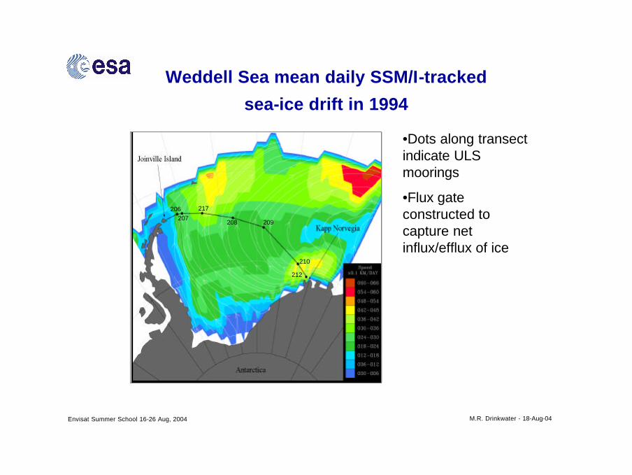
Weddell Sea mean daily SSM/I-tracked

sea-ice drift in 1994

•Dots along transect indicate ULS moorings

•Flux gate constructed to capture net influx/efflux of ice

206207

217

208 209

210

212


Volume Transport <Vice* Hice> at ULS moorings

• Flux computed in transport per unit width at each ULS mooring location

• Shading indicates error bars, or uncertainties based on the uncertainties in the ULS draft measurement (and draft to thickness conversion); the velocity tracking errors

• Peak Transport in austral winter, as the second year ice is advected over the ULS locations

• Central gyre has a very small seasonal cycle

• Western Weddell (207, 217) indicates peak transport exceeding 0.3 m3/s per unit length in 1991

inflow

outflow


Daily Net Sea Ice Area Flux

• Plot shows daily variability in net flux.

• Oscillations on day-to-day basis extremely large, with drift reversals changing sign of net flux of ice

• Net Mean Area export of ~757,000 km2/yr

• Models need to cope with highly dynamic flux environment

2


(a) SSM/I-derived Net monthly area flux and (b) combined net volume flux (annual means (solid circles) after Harms et al.)

• Monthly means yield 10 year mean ice export of 31,530 m3/year (indicated by dotted line)

• Significant seasonal-interannual variability in flux

• Quasi-quadrennial periodicity in net transport, as related to interannual SLP variations observed by Venegas et al (2001)


Mean 1992 Ice Volume Transportper unit length along transect

1 m3/s = 0.032 km3/y


Freshwater Budget

•Ice volume converted to freshwater using typical ice density of 910 kg/m3 and thickness related salinity value

•Principal sources of freshwater are:

Precip – Evap (~50%)Gyre import (~25%)Ice shelf/iceberg melt(~25%)

•Data valuable to assess regional model performance


Remaining Challenges:

- Sub-Daily Ice Motion- Data Assimilation


What’s Hidden in the Drift?

• Typical SAR-tracked 3d ice drift at Ice Station Weddell indicates predominantly northwards translation, with periodic rotation events

• Drift from Crossing orbits at sub-daily intervals uniquely indicate large amount of rotation in the ice pack

• The shorter the interval, the greater the rotational component

• Are intertial/tidal velocities aliased into the drift velocity?


Tidal/inertial residual (after removal of mean drift)


• Ascending/Descending combinations with sub-daily intervals indicate significant aliased residual motion• Residual drift illustrates anticlockwise rotation over varying sub-daily intervals• Exact repeat orbits (during ice phase) do not alias tidal/inertial oscillations


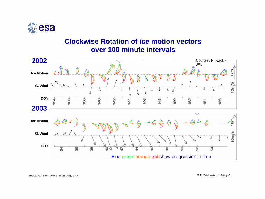
Clockwise Rotation of ice motion vectors over 100 minute intervals

Ice Motion

G. Wind

DOY

2002

2003

Blue-green-orange-red show progression in time

Ice Motion

G. Wind

DOY

Courtesy R. Kwok -JPL


Semi-diurnal Oscillation in Divergence

Oscillation superimposed on lower freq wind-driven component

Courtesy R. Kwok -JPL


SUMMARY (2)

• Tracking technology and ice drift applications of SSM/I and Scatterometer data have extended the applicability of these sea-ice data to:

• Ice Drift - Freshwater Flux Estimates• Ice Dynamics - Opening/Closing modulates air-sea fluxes and salt

production in the polar oceans

• Ice kinematics data allow definition of length- and time-scales of the response of the sea-ice cover to atmospheric and oceanographic forcing.

• Data available for assimilation and/or model performance verification

• Comparisons of satellite ice motion with ECMWF and NCEP data highlight significant problems with Antarctic meteorological analyses

• Interannual adjustments in ice dynamics in response to variability in basin-wide atmospheric forcing. Strong links to AO, NAO, ENSO, and other such oscillation patterns

• Variable freshwater export modulates thermohaline circulation inNorth Atlantic and Weddell Sea


Commentary• SAR brought us efficient tracking algorithms and infused the polar

community with new technology and insight into polar processes • Scatterometers yield an extremely valuable climatological radar

database - as yet under appreciated and underused– C-band Scatt continuity on METOP for next 15 yrs (2005 – onwards).

• Polar community has been too focused on use and application of high-resolution SAR products. Flight agencies MUST embrace wider use of low resolution, long-time sequence, global radar data sets in geophysical studies.

– Effective resolution of scatterometers is complementary to passive microwave sensors.

• Weather effects remain a critical limitation to SSMI/AMSR during“events” forcing the ice cover. Clever approaches are required to mitigate these problems

• The future is multi-platform data fusion (SAR + Passive Microwave + Scatterometer + Altimeter) and assimilation of polar products in GCMs

• A global (Wide-Swath) sea-ice radar mission is required to generate a dedicated high-resolution data set with which to address sub-daily processes in response to storm and tidal forcing.


Sea-Ice Drift Data Resources

• New Antarctic SSMI + buoy Ice Drift Atlas– http://imkhp7.physik.uni-

karlsruhe.de/~eisatlas/HTML/eisatlas_products.html

• Satellite Drift Products– Polar Pathfinder Products:

• http://nsidc.org/data/nsidc-0116.html

– IFREMER/CERSAT Scatterometer Arctic Ice Drift products• http://www.ifremer.fr/cersat/en/data/overview/gridded/psidrift.ht

m– JPL RGPS/SSMI ice drift products

• http://www-radar.jpl.nasa.gov/rgps/


A short course on sea ice data assimilation was held at the Naval Academy, Annapolis, MD on July

23-24, 2002

Further info – incl. Course materialis available at:

http://ecco.jpl.nasa.gov/sea_ice/or contact Dimitris Menemlis @JPL

Date post:	11-Apr-2018
Category:	Documents
Upload:	truongnhu
View:	218 times
Download:	1 times

Scientific Challenges Associated with Sea Ice-Drift … · Scientific Challenges Associated with...

Documents