University of Wisconsin MilwaukeeUWM Digital Commons

Theses and Dissertations

December 2012

SCR-Based Wind Energy Conversion Circuitryand Controls for DC Distributed Wind FarmsRavi NanayakkaraUniversity of Wisconsin-Milwaukee

Follow this and additional works at: https://dc.uwm.edu/etdPart of the Electrical and Electronics Commons

This Dissertation is brought to you for free and open access by UWM Digital Commons. It has been accepted for inclusion in Theses and Dissertationsby an authorized administrator of UWM Digital Commons. For more information, please contact open-access@uwm.edu.

Recommended CitationNanayakkara, Ravi, "SCR-Based Wind Energy Conversion Circuitry and Controls for DC Distributed Wind Farms" (2012). Theses andDissertations. 63.https://dc.uwm.edu/etd/63

SCR-BASED WIND ENERGY CONVERSION CIRCUITRY AND CONTROLS FOR

DC DISTRIBUTED WIND FARMS

By

Ravi Nanayakkara

A Dissertation Submitted in

Partial Fulfillment of the

Requirements for the Degree of

Doctor of Philosophy

in Engineering

at

The University of Wisconsin-Milwaukee

December 2012

ii

ABSTRACT

SCR-BASED WIND ENERGY CONVERSION CIRCUITRY AND CONTROLS FOR

DC DISTRIBUTED WIND FARMS

By

Ravi Nanayakkara

The University of Wisconsin-Milwaukee, 2012

Under the Supervision of Professor Adel Nasiri

The current state of art for electrical power generated by wind generators are in

alternating current (AC). Wind farms distribute this power as 3-phase AC. There are

inherent stability issues with AC power distribution. The grid power transfer capacity is

limited by the distance and characteristic impedance of the lines. Furthermore, wind

generators have to implement complicated, costly, and inefficient back-to-back

converters to generate AC. AC distribution does not offer an easy integration of energy

storage. To mitigate drawbacks with AC generation and distribution, direct current (DC)

generation and high voltage direct current (HVDC) distribution for the wind farms is

proposed. DC power distribution is inherently stable. The generators convert AC power

to DC without the use of a back-to-back converter. DC grid offers an easy integration of

energy storage.

iii

The proposed configuration for the generator is connected to a HVDC bus using a 12

pulse thyristor network, which can apply Maximum Power Point Tracking (MPPT). To

properly control the system, several estimators are designed and applied. This includes a

firing angle, generator output voltage, and DC current estimators to reduce noise effects.

A DSP-based controller is designed and implemented to control the system and provide

gate pulses. Performance of the proposed system under faults and drive train torque

pulsation are analyzed as well. Additionally, converter paralleling when turbines operate

at different electrical power levels are also studied. The proposed new Wind Energy

Conversion System (WECS) is described in detail and verified using MATLAB®/

Simulink® simulation and experimental test setup. The proposed solution offers higher

reliability, lower conversion power loss, and lower cost. The following is proposed as

future work:

1) Study different control methods for controlling the SCR’s.

2) Investigate reducing torque pulsations of the PMSG and using the proposed

power conversion method for DFIG turbines.

3) Explore options for communication/control between PMSG, circuit protection

and grid-tied inverters.

4) Investigate the best possible configuration for DC storage/connection to the

HVDC/MVDC bus.

5) Study the filtering needed to improve the DC bus voltage at the generator.

iv

© Copyright by Ravi Nanayakkara, 2012

All Rights Reserved

v

To my daughter and son

vi

TABLE OF CONTENTS

ACKNOWLEDGEMENTS ......................................................................................... xvi 

LIST OF ABBREVIATIONS ..................................................................................... xvii 

Chapter 1 ............................................................................................................................. 1 

1.0 Wind Energy ............................................................................................................. 1 

1.1 Environmental Impact ............................................................................................... 2 

1.2 Wind Generators. ...................................................................................................... 3 

1.3 Power Electronics ...................................................................................................... 6 

1.4 Statement of thesis subject ........................................................................................ 8 

1.5 Proposed solution ...................................................................................................... 9 

1.6 Configuration of the proposed solution ..................................................................... 9 

1.7 Prior art .................................................................................................................... 10 

1.8 Thesis organization ................................................................................................. 11 

Chapter 2 ........................................................................................................................... 12 

2.0 HVDC/MVDC SYSTEMS ..................................................................................... 12 

2.2 HVDC Sytem. ......................................................................................................... 13 

2.3 Current source converter ......................................................................................... 15 

2.4 Voltage source converter ......................................................................................... 16 

2.5 HVDC Distribution. ................................................................................................ 19 

2.4 Bipole fault operation .............................................................................................. 24 

vii

Chapter 3 ........................................................................................................................... 26 

3. 0 System architecture and modeling ......................................................................... 26 

3.1 System architecture ................................................................................................. 26 

3.2 Thyristor Power converter ....................................................................................... 29 

3. 3 Power converter -12 pulse ...................................................................................... 31 

3.4 Phase firing of the 12 pulse SCR ............................................................................ 33 

3.5 HVDC bus power flow ............................................................................................ 34 

3.3 Step up transformer ................................................................................................. 35 

3.4 DFIG........................................................................................................................ 35 

3.4 Modeling ................................................................................................................. 36 

3.5 Wind Turbine model ............................................................................................... 38 

3.6 PMSG Model........................................................................................................... 40 

3.7 Vd,Vq estimator........................................................................................................ 42 

3.8 HVDC Vdr,Vqr estimator ....................................................................................... 43 

3.9 Step up transformer ................................................................................................. 44 

3.10 SCR converter ....................................................................................................... 45 

3.11 PI Current regulator ............................................................................................... 47 

3.12 SCR Pulse generator.............................................................................................. 48 

3.13 Simulation results .................................................................................................. 48 

Chapter 4 ........................................................................................................................... 54 

viii

4.0 Estimation of Alpha, DC current, and AC voltage ................................................. 54 

4.1 Control system......................................................................................................... 54 

4.2 Vq - Vd Estimator..................................................................................................... 55 

4.3 Vqr –Vdr Estimator ................................................................................................. 59 

4.4 SCR Converter – 6 pulse ......................................................................................... 63 

Chapter 5 ........................................................................................................................... 66 

5.0 Experimental test setup ........................................................................................... 66 

5.1 Lab setup ................................................................................................................. 66 

5.2 Power Section .......................................................................................................... 67 

5.3 Control section ........................................................................................................ 70 

5.4 Simulink DSP programming ................................................................................... 71 

5.5 Hardware setup results ............................................................................................ 79 

Chapter 6 ........................................................................................................................... 90 

6.0 Maximum Power Point Tracking (MPPT) .............................................................. 90 

6.1 Wind regions of operation ....................................................................................... 90 

6.2 Capture of wind energy. .......................................................................................... 91 

6.3 Wind generator mechanical equations. ................................................................... 94 

6.4 Simulation results .................................................................................................... 97 

Chapter 7 ........................................................................................................................... 98 

7.0 Paralleling of wind generators, Fault analysis and Torque pulsations. ................... 98 

ix

7.1 Wind farm operation ............................................................................................... 98 

7.2 Faults Analysis ...................................................................................................... 101 

7.3 Torque pulsation .................................................................................................... 104 

Chapter 8 ......................................................................................................................... 106 

8.1 DC Power inversion to Grid .................................................................................. 106 

8.2 Selection of the inverter, converter and filter topologies ...................................... 106 

8.3 Control of grid side inverter .................................................................................. 107 

8.3 Frequency droop and voltage droop control ......................................................... 108 

Chapter 9 ......................................................................................................................... 110 

9.0 Conclusion ............................................................................................................. 110 

References ....................................................................................................................... 114 

CURRICULUM VITAE ............................................................................................. 119 

x

LIST OF FIGURES

Figure 1. 1 The configuration of a typical wind turbine. .................................................... 4 

Figure 1.2 Different configurations of wind turbines with different generators. ................ 5 

Figure 1.3 A single phase circuitry of a soft starter. ........................................................... 7 

Figure 1.4 The circuitry of a back to back converter. ......................................................... 8 

Figure 1.5 Architecture of the proposed wind energy conversion system. ......................... 9 

Figure 2.1 HVDC System. ............................................................................................... 14 

Figure 2.2 Current Source Converter. ............................................................................... 15 

Figure 2.3 CSC with 6 SCR and firing order. ................................................................... 15 

Figure 2.4 Voltage Source Converter. .............................................................................. 16 

Figure 2.5 VSC Four quadrant operation. ......................................................................... 17 

Figure 2.6 Monopole distribution. .................................................................................... 19 

Figure 2.7 Monopole distribution with low voltage return. .............................................. 20 

Figure 2.8 Bipolar Distribution. ........................................................................................ 21 

Figure 2.9 Bipolar distribution with dedicated ground return. ......................................... 22 

Figure 2.10 Meshed DC systems. ..................................................................................... 23 

Figure 2.11 Configuration of a HVDC system under overhead line fault. ....................... 24 

Figure2.12 Configuration of a HVDC system underground return fault. ......................... 24 

Figure 3.1 System architecture for the proposed DC distribution. ................................... 27 

Figure 3.2 PMSG, “STAR-DELTA” transformer and 12-pulse SCR configuration. ....... 28 

xi

Figure 3.3 Electrical symbol of an SCR. .......................................................................... 30 

Figure 3.4 300 Phase shift between star and delta winding.............................................. 32 

Figure 3.5 Phase firing of SCR’s ..................................................................................... 33 

Figure 3.6 Converter power flow for the 12-pulse rectifier. ............................................ 34 

Figure 3.7 Proposed SCR-based rectifier for DFIG wind turbine. .................................. 36 

Figure 3.8 Complete configuration of the system in Simulink® environment. ................ 37 

Figure 3.9 Simulink® Wind turbine model. ..................................................................... 39 

Figure 3.10 Simulink® Wind turbine model parameters. ................................................. 39 

Figure 3.11 Turbine Power Characteristics (MATLAB®/ Simulink®). .......................... 40 

Figure 3.12 MATLAB®/ Simulink® PMSG model. ....................................................... 40 

Figure 3.13 PMSG measured and estimated voltage. ....................................................... 43 

Figure 3.14 HVDC Vdr,Vqr estimator. ............................................................................ 44 

Figure 3.15 Star-Delta transformer. .................................................................................. 44 

Figure 3.16 Transformer parameters. ................................................................................ 45 

Figure 3.17 MATLAB®/ Simulink® model of an SCR module. ..................................... 46 

Figure 3.18 SCR firing order. ........................................................................................... 47 

Figure 3.19 current regulator with firing angle modulation. ............................................ 47 

Figure 3.20 SCR firing module. ........................................................................................ 48 

Figure 3.21 Estimated alpha, Estimated Vqr, Estimated Iqr , Estimated Idr and wind

speed. ................................................................................................................................ 49 

xii

Figure 3.22 Measured Voltage, Estimated voltage, Measured Current, Estimated current

and wind speed. ................................................................................................................. 50 

Figure 3.23 PMSG Estimated Vd voltage, Estimated Vq voltage, measured current Id, Iq

and wind speed. ................................................................................................................. 51 

Figure 3.24 Firing angle, Estimated Alpha, Reference DC current, HVDC Current and

wind speed. ....................................................................................................................... 52 

Figure 3.25 DC Bus voltage, 3 phase line to line voltage of PMSG, 3 phase current of

PMSG and DC current. ..................................................................................................... 53 

Figure 4.1 PMSG Control system. .................................................................................... 54 

Figure 4.2 d-q axis representation of a PMSG machine. .................................................. 56 

Figure 4.3 Vqr-Vdr estimator .............................................................................................. 58 

Figure 4.4 d-q and dr –qr axis relationship. ....................................................................... 61 

Figure 4.5 Vqr –Vdr Estimator. ........................................................................................ 62 

Figure 4.6 d-q and dr-qr representation of the PMSG and SCR converter. ...................... 63 

Figure 5.1 A picture of the lab setup showing SCRs, transformers, and control boards. . 66 

Figure 5.2 Block diagram of the test setup. ...................................................................... 67 

Figure 5.3 SCR connection. .............................................................................................. 67 

Figure 5.4 12 pulse SCR connection. ................................................................................ 68 

Figure 5.5 Star-Star connections. ...................................................................................... 69 

Figure 5.6 Star-Delta connections. .................................................................................... 69 

Figure 5.7 DSP Program flow ........................................................................................... 71 

xiii

Figure 5.8 Calculation of Tcap time in the DSP module. ................................................. 73 

Figure 5.8 Valid capture of Tcap time flow diagram. ....................................................... 74 

Figure 5.9 Interrupt routine for the DSP for real time control. ......................................... 74 

Figure 5.10MATLAB®/ Simulink® code for SCR firing circuit. .................................. 76 

Figure 5.11 SCR firing pattern vs angle. ......................................................................... 77 

Figure 5.12 DSP Vabc estimated results of 3 phase voltage. .......................................... 79 

Figure 5.13 DSP Vqr-Vdr estimator results of HVDC current read via a serial port. ....... 80 

Figure 5.14 DSP Alpha estimator results read back via a serial port. ............................. 81 

Figure 5.15 Green DC bus voltage, Blue AC voltage, Magenta .................................... 83 

Figure 5.16 Green DC bus voltage, Blue AC voltage, Magenta synchronizing signal,

frequency 24.23 Hz. .......................................................................................................... 83 

Figure 5.17 Green DC bus voltage, Blue AC voltage, Magenta synchronizing signal,

frequency 35.05 Hz. .......................................................................................................... 84 

Figure 5.18 Green DC bus voltage, Blue AC voltage, Magenta synchronizing signal,

frequency 43.15 Hz. .......................................................................................................... 84 

Figure 5.19 Green DC bus voltage, Blue AC voltage, Magenta synchronizing signal,

frequency 53.19 Hz. .......................................................................................................... 85 

Figure 5.20 Blue DC bus voltage, Red AC voltage, Green DC current, Magenta AC

current. .............................................................................................................................. 86 

Figure 5.21 Blue DC bus voltage, Red AC voltage, Green DC current, Magenta AC

current. .............................................................................................................................. 87 

xiv

Figure 5.22 Lab setup of the complete system connected to a AC generator. .................. 88 

Figure 5.23 Red DC bus voltage, Blue AC Voltage, Magenta AC current and Green is

DC current. ........................................................................................................................ 89 

Figure 6.1 Wind Turbine regions of operation. ................................................................ 90 

Figure 6.2 Wind turbine output power versus Tip-Speed Ratio (TSR). ........................... 93 

Figure 6.3 Wind turbine output power versus rotor speed. ............................................... 94 

Figure 6.4 Wind Turbine mechanical system of power transfer. ...................................... 95 

Figure 6.5 Configuration of the MPPT Control system. ................................................... 96 

Figure 6.6 MPPT Simulation results for changing wind speed. ....................................... 97 

Figure 7.1 Configuration of the proposed DC distributed PMSG wind farm with multi-

terminal interconnections. ................................................................................................. 98 

Figure 7.2 Simulation configuration of Parallel wind generators to a common DC bus. . 99 

Figure 7.3 Simulation of parallel wind generators connected to a common DC bus. ... 100 

Figure 7.4 Configuration of the proposed AC fault isolation with AC breakers. .......... 102 

Figure 7.5 Simulation of a ground fault on this system. ................................................ 103 

Figure 7.6 Simulation of torque pulsations. ................................................................... 105 

Figure 8.1 Wind energy conversion system with energy storage. .................................. 109 

xv

LIST OF TABLES

Table 1.1. Comparison of different types of wind turbine. ................................................. 6 

Table 2.1 Comparison of the two converter topologies [13] ............................................ 18 

Table 3.1 Turbine Parameters. .......................................................................................... 38 

xvi

ACKNOWLEDGEMENTS

I would like to thank my thesis advisor, Dr Adel Nasiri for his guidance, knowledge and

encouragement. I Would also like to thank my dissertation committee: Dr. David Yu, Dr.

Jugal Ghorai, Dr. Mahsa Ranji and Dr. Al Ghorbanpoor. Without their advice this thesis

would not be possible. I would like to thank Rockwell Automation, my employer for

supporting me with hardware for the lab setup. This allowed me to build the prototype

system rapidly.

I also thank my fellow colleagues Bora Novakovic, Zeljko Jankovic, Ahmad Hamidi and

Goran Mandic for their help with the project.

I appreciate the tedious task of proof reading by my parents Amarasena and Padma

Nanayakkara, Dineshi Burchi and Georgia Hill.

Finally, I thank my family for encouragement, understanding and support.

xvii

LIST OF ABBREVIATIONS

HVDC – High Voltage Direct Current

MVDC – Medium Voltage Direct Current

DC – Direct Current

AC – Alternating Current

SCR – Silicon Controlled Rectifier

VSC – Voltage Source Converter

CSC – Current Source Converter

PMSG – Permanent Magnet Synchronous Generator

MPPT – Maximum Power Point Tracking

PE – Power Electronic

RMS – Root Mean Square

WECS- Wind Energy Conversion systems

DFIG –Doubly Fed Induction Generator

DSP –Digital Signal Processor

1

Chapter 1

1.0 Wind Energy

Wind Energy is becoming a sizeable contributor to the ever-expanding energy

market. Given the impact on the environment from the use of fossil fuels, there is even a

bigger interest in alternative energy sources today [1]. Wind energy is proven as a viable

source of clean energy. Over the past decade, there had been numerous advances in the

design, control, fault tolerance, and power distribution associated with Wind Energy

Conversion systems (WECS).

According to American Wind Energy Association (AWEA), 48,611 MW of wind power

capacity was installed in the U.S as of first quarter 2012. This represents 20% of world’s

installed wind power capacity. The U.S wind industry has added over 35% of all new

generating wind power capacity in the last 5 years. U.S is also well suited for wind

energy penetration. There is a massive demand for electrical energy as well as an

abundance of wind resources. The wind potential is one of the best in the world. It is

estimated that the wind capacity is in the range of 37 trillion kilowatt hours of electricity

annually. This is 10 times the existing power requirements of the country.

The U.S Department of Energy and National Renewable Energy Laboratory has studied

the scenario of 20% wind energy by 2030. It also contrast not adding any new wind

power capacity by 2030. To meet this goal, wind power capacity would have to be

increased to 16,000 MW per year by 2018, and grow at this rate until 2030. It also

assumes that the prevailing technology is sufficient to meet this demand. The net result

of this study is that U.S energy production would be diversified and wind electricity

2

would stabilize the energy markets from volatile price swings. This also would greatly

reduce the dependence of foreign energy sources.

Currently the following states in the U.S. lead in wind energy production. Texas 10,085

MW, Iowa 3,675 MW, California 3,177 MW, Minnesota 2,192 MW and Washington

2,104 MW. Offshore wind is a new opportunity for US. The first offshore wind farm

was established off the coat of Denmark. It is estimated by the National Renewable

Energy Laboratory (NREL) that the estimated offshore capacity is 4 times the country’s

current generating capacity from all sources. Other countries in the world have taken lead

in increasing the off shore wind capacity. Europe is planning to have 40,000 MW of

wind power by 2015 and China is planning 30,000 MW of installed capacity by 2015.

1.1 Environmental Impact

Wind energy produces zero emissions in generating power from the wind. Electricity

generation in the U.S. is one of the largest sources of air pollution. It is estimated that

40% of Co2 emissions are generated by power generation facilities. The AWEA has

suggested that if a 20% of total energy is generated by wind energy by 2030, it would

reduce Co2 emissions by 825 million metric tons. This is a real benefit to reducing

greenhouse gasses that are directly linked to increasing global warming.

3

1.2 Wind Generators.

We have been harnessing the power of wind for many years. Wind mills have been used

to pump water and grind grain. The first modern wind turbine was built in 1957. Gedser

wind turbine was 200 kW wind turbine with horizontal axis and three blades connected to

a three phase AC grid [26] . Many different concepts and technology have been tested

since. During 1970’s, due to oil crises, the small wind turbines (22 kW) were built using

inexpensive parts for house hold applications.

In the last three decades, wind turbine rating has increased from 20 kW to 5 MW. The

new concepts such as pitch control and variable speed control methods have been

developed and introduced to the wind industry. Since 1993, wind turbine manufacturers

have changed the generator from the AC induction generator to the synchronous

generator and induction generator with wounded rotor. The new machines have better

capability of handling power in the wind turbine systems [26].

The progression of power electronics both in switches with better power handling

capability and cost/kW encourages the manufacturers to employ sophisticated power

electronic equipment. In fact, power electronics is the basis for most new developments

in wind turbines [26].

Figure 1.1 shows the configuration of a simple wind turbine. A wind turbine simply

consists of blades, a generator, a power electronic converter, and power grid. Sometimes,

wind turbine work in islanding mode; therefore, there is no grid. Usually, there are two or

three blades on a wind turbine. There were some wind turbines with more than three

4

blades. But based on aerodynamics, three blades is the optimum number of blades for a

wind turbine [27].

Asynchronous and synchronous AC machines are the main generators that are used in the

wind turbines. Based on the generator, the form of the connections of the machine to the

grid and the drive method of the generator, there are numerous wind turbine

configurations. Besides that, manufacturers may use their own configuration to overcome

the high price of the equipment, design constraints and other regulations.

Figure 1. 1 The configuration of a typical wind turbine.

Figure 1.2 shows several configurations of the wind turbines. Type A uses the AC

induction generator. There is also a gearbox to drive the generator. This type is the most

common wind turbine in the wind farms. Type B is called the Doubly Fed Induction

Generator (DFIG) wind turbine. The wounded induction generator is used. A power

electronic converter is used to feed the rotor windings of the generator. The generator is

driven by a gearbox. Type C uses Permanent Magnet Synchronous Generator (PMSG). If

a gearbox is not used, it is called direct driven wind turbine. A full range power

5

converter is used to connect the generator to the grid. Table 1.1 compares these

configuration in different aspects [26].

Type A

Type B

Type C

Figure 1.2 Different configurations of wind turbines with different generators.

6

Table 1.1. Comparison of different types of wind turbine.

Configuration PE converter Drive Operation

A Soft starter Gearbox Fixed speed

B Back-to-back

converter

Gearbox Variable speed

C Back-to-back

converter

Direct Variable speed

1.3 Power Electronics

As the advanced technology invents high current and voltage power switches, application

of the Power Electronic (PE) converter increases in the industry. Power electronic

equipment is an attractive means to improve the performance of wind turbines. Many

types of power converters are used in the wind industry. The power converter must be

capable of connecting an AC source that is variable voltage and frequency to a fixed

voltage and frequency.

The soft starter is a type of power converter that is used with induction machines in fixed

speed wind turbines. It reduces the transient current during the startup period of a wind

turbine. Figure 1.3 shows a soft starter for one phase. When the speed of the generator is

more than the synchronous speed, the soft starter connects the generator to the grid

7

smoothly, using the firing angle of the thyristors. When the generator is fully connected,

the thyristors will be bypassed by a bypass switch.

Figure 1.3 A single phase circuitry of a soft starter.

A Back-to-Back Converter (BBC) is another type of power electronic converter that is

used in the wind industry. Figure 1.4 shows a back to back converter circuitry. It consists

of a PWM rectifier and a PWM inverter. Therefore, the AC input voltage of the generator

is first rectified and then converts into AC using the inverter. A BBC is a very powerful

PE converter and is capable of controlling active and reactive power. Therefore, it is

used in a variable speed wind turbine. The rectifier sometimes is called generator side

converter and the inverter is called grid side converter.

8

Figure 1.4 The circuitry of a back to back converter.

Besides the PE converters that are mentioned above, there are other PE converters that

can be used such as Matrix converters, capacitor banks, Tandem converters, Multi-level

converters, etc. [43].

1.4 Statement of thesis subject

• The electrical power generated by the wind generator are alternating current (AC).

• AWind farm power distribution is 3-phase AC. An offshore wind farm or a wind

farm located far from the energy consumers would have to distribute the power

generated using a 3-phase grid connection.

• There are inherent stability issues with AC power distribution. AC distribution

does not offer an easy integration of energy storage.

• The power transfer capacity of AC lines is limited.

• Wind generators have to implement complicated, costly, and inefficient back- to -

back converters to implement AC generation.

9

1.5 Proposed solution

• The wind turbine output power is in DC form after SCR-based rectification.

• Wind farm power distribution is HVDC/MVDC . An offshore wind farm or a

wind farm located far from the energy consumers would distribute the power

generated using DC grid connection.

• DC power distribution is inherently more stable.

• Wind generators convert AC to HVDC directly without a back-to-back converter.

• DC grid offers an easy integration of energy storage.

1.6 Configuration of the proposed solution

Figure 1.5 Architecture of the proposed wind energy conversion system.

10

The proposed solution is to convert the AC voltage generated by the wind generators to

HVDC. A common HVDC bus would be used to distribute this power to the grid via

inverters. DC storage can be easily integrated to the HVDC bus. This will allow the

stabilization and smoothing of grid voltage. The nacelle of the wind generator is made

lighter by bringing the power converter and associated circuitry to the base of the tower.

This would allow easy access for maintenance. The proposed solution is fully simulated

and a hardware setup is built to verify this proposed system and control.

1.7 Prior art

The current technology related to wind generators and use of HVDC as distribution in

literature is limited to all generators having a back-to-back converter or the conversion of

AC power to DC using a voltage source converter. The AC power is then converted to

HVDC for distribution. In [6] a line commutated HVDC bus is introduced. Also the

optimal condition for DC power distribution is discussed, but generators still used

produce AC power and not DC. In the paper [16] the controls of a DFIG system

connected to a HVDC are discussed. STATCOM is used to support the generator side

grid. In [17] Voltage source converters are used per generator to convert AC to DC.

HVDC light is used as the distribution method. In[18] Current Source Inverters are

ganged together to produce HVDC.

11

1.8 Thesis organization

The thesis is organized in to the following chapters:

• Introduction on wind energy and need for DC wind farms.

• HVDC systems.

• System architecture and modeling.

• Estimation of Alpha, HVDC Currents and PMSG voltage.

• System Implementation and control.

• Maximum Power point tracking.

• Paralleling of wind generators.

• DC Power inversion to Grid.

12

Chapter 2

2.0 HVDC/MVDC SYSTEMS

Note: High Voltage Direct Current (HVDC) or Medium Voltage Direct Current(MVDC)

will be referred as HVDC in this chapter.

HVDC systems have been in existence since the early 1930’s with the advent of mercury

arc rectifiers. Today HVDC technology is considered mature, and is used for

transmission of bulk power. The transmission and distribution of electrical energy

started with direct current. The first know transmission link was built in Germany in

1882. It was capable of transmitting at 2kV for 50 km. One issue faced was the

conversion of DC voltage levels to lower consumer levels. This was accomplished by

using rotating DC machines. On the other hand, AC voltage conversion was easily

accomplished by using a transformer. This was a simple low cost device. AC three-

phase generation using synchronous generators is far more superior to DC generation.

These reasons led to the early adaptation of AC distribution.

However, high voltage AC generations has many disadvantages.[28]

• Transmission capacity is limited by inductive and capacitive elements of the

overhead lines and cables and the distance power can be transmitted.

• Charging currents limit the distance of transmission from 40 to 100 km.

• Connecting two different AC systems with different frequencies is not possible.

13

HVDC Transmission advantages.

• DC link allows transmission of power between different AC networks.

• DC conductor is fully utilized. There is no skin effect.

• Transmission distance is not limited by inductive and capacitive elements in the

cable.

• For power distribution of 40 km and above, the only solution is HVDC. The

charging currents of AC cable limits the distance the power can be distributed.

• For wind generation the DC link eliminates the flicker due to wind turbulence and

tower shadow.

• DC cables need less space and can carry more power than AC cables.

2.2 HVDC Sytem.

The HVDC transmission system consist of a AC to DC converter, HVDC Line and DC

to AC inverter. Figure 2.1 gives this representation [28].

14

Figure 2.1 HVDC System.

The power flow or the current flow is only in one direction. The power will flow from the

converter to the inverter. This is accomplished by controlling the voltage at the

converter. There are two main converter topologies that are used today to the converter 3

phase AC to DC [13].

• Current source converter (CSC)

• Voltage source converter (VSC)

15

2.3 Current source converter

Current source converters use SCR as a fundamental switching device. In the early days,

mercury arc valves were used. A current source converter converts a constant voltage

source in to a current source. Figure 2.2 shows the overview of such a system [13].

Figure 2.2 Current Source Converter.

The building block for a CSC is 6 SCR connected to a 3-phase balanced AC system as

following in figure 2.3.

Figure 2.3 CSC with 6 SCR and firing order.

16

Due to the inductance, the 6-bridge SCR would overlap. At any given time two or three

valves can overlap. It can be shown that the converter DC voltage that is rectified is equal

to 1.35 VLL where the VLL is the line-to-line voltage of the 3-phase system. The SCR

are line commutating. Therefore, only the turn on angle in relationship to the forward

biasing voltage can be adjusted to change the output DC voltage.

2.4 Voltage source converter

A voltage source converter uses a IGBT or GTO as switching devices. These devices can

be forced commutated as shown in figure 2.4 [12].

Figure 2.4 Voltage Source Converter.

This allows the switch to be turned on-off anywhere in the cycle. Therefore, these

devices are PWM at a higher frequency than the line frequency of the system.

The VSC convert can operate in four quadrants. Either rectifier/inverter with leading or

lagging power factor. This is given in figure 2.5.

17

Figure 2.5 VSC Four quadrant operation.

We can compare the advantages and disadvantages of the two topologies. These are given

in the table below.

18

Table 2.1 Comparison of the two converter topologies [13]

Converter type

CSC VSC

AC Side Acts like a constant voltage source. Acts like a constant current source.

Requires a capacitor as energy storage.

Requires an inductor as its energy storing device.

Requires filters for harmonic elimination.

requires a small filter for harmonic elimination.

Requires reactive power supply for power factor correction.

Reactive power supply is not required.

DC side Acts like a constant current source. Acts like a constant voltage source.

Requires an inductor as its energy storage. Requires capacitor as energy storage.

Requires DC filters. Capacitor provides DC filtering.

Provides inherent fault current limit.

Problamatic for DC line side shorts faults since the charge capacitor will discharge in to fault.

Switches Line or force commutated with series capacitor. Self -Commutaed.

Switching occurs at line frequency Switching occurs at high frequency.

Lower switching losses. Higher switching losses.

Rating 0-500 MW per converter 0-200 MW per Converter.

Upto 600kV Upto 100kV

19

2.5 HVDC Distribution.

HVDC systems can be configured in many ways for distribution.

• Monopole Distribution.

The monopole distribution system uses a single over head or marine cable for DC power

distribution. The ground is used as a return path. If the ground cannot be used for a

return path a low voltage dedicated metal return path can be used. These two

configuration are given in figures 2.6 and figure 2.7[28].

Figure 2.6 Monopole distribution.

20

Figure 2.7 Monopole distribution with low voltage return.

• Electrochemical corrosion of long buried metal objects such as pipelines is a

concern with this system.

• Underwater earth-return electrodes in seawater may produce chlorine or otherwise

affect the water chemistry.

• An unbalanced current path may result in a net magnetic field, which can affect

magnetic navigational compasses for ships passing over an underwater cable.

• Modern monopole systems for pure overhead lines carry typically 1,500 MW. If

underground or underwater cables are used, the typical value is 600 MW.

21

• Bipolar Distribution.

The bipolar uses two poles and uses two high voltage lines for power distribution. The

main advantage is that you can transmit twice the power compared to a monopole

configuration. In this configuration there is negligible current flowing in the ground

return path. A dedicated ground return cable can be added to this configuration. These

two configurations are given in figure 2.8 and figure 2.9.

Figure 2.8 Bipolar Distribution.

22

InverterConverter

HVDC Cable

HVDC Cable

LVDC Cable

Figure 2.9 Bipolar distribution with dedicated ground return.

Under a normal load, negligible earth-current flows, as in the case of monopolar

transmission with a metallic earth-return. This reduces earth return loss and

environmental effects.

When a fault develops in a line, with earth return electrodes installed at each end of the

line, approximately half of the rated power can continue to flow using the earth as a

return path, operating in monopolar mode.

Due to the fact that for a given total power rating, each conductor of a bipolar line carries

only half the current of monopolar lines, the cost of the second conductor is reduced

compared to a monopolar line of the same rating.

23

In a very adverse terrain, the second conductor may be carried on an independent set of

transmission towers, so that some power may continue to be transmitted, even if one line

is damaged.

Bipolar systems may carry as much as 3,200 MW at voltages of +/-600 kV. Submarine

cable installations initially commissioned as a monopole may be upgraded with

additional cables and operated as a bipole.

• Multi-terminal DC distribution

Multi-terminal DC distribution is considered in urban areas were space is limited. It is

similar to AC distribution system. This is a meshed DC system. It is given in figure

2.10. As we can see, we can use a common DC bus to do DC distribution to urban city

centers. The power from alternative energy sources like wind and solar can be converted

back to AC [13].

=~

=~

=~

=~

DC Bus

Figure 2.10 Meshed DC systems.

24

2.4 Bipole fault operation

It is necessary to understand the robustness of the system. Part of that analysis is to

understand kinds of faults can be tolerated by the system. In the case of a bipole

configured system there can be two types of faults. This is depicted in the following

figures 2.11,2.12 [28].

Figure 2.11 Configuration of a HVDC system under overhead line fault.

Figure2.12 Configuration of a HVDC system underground return fault.

25

• Overhead line fault – Transmit in monopole configuration using the ground

return.

• Ground return fault- Transmit in monopole configuration using the overhead line

as return.

Both modes will transmit 50% of power.

It is important to have redundancy in the system. This is a crucial consideration in

building a HVDC system so power can be transmitted from the point of generation to the

consumers.

26

Chapter 3

3. 0 System architecture and modeling

3.1 System architecture

Modern PMSG generators are variable speed generators allowing the generation

of power from variable wind. This is possible due to a back-to-back power electronic

converter. This allows variable frequency AC to be converted to DC and inverted back to

AC synchronized to the grid frequency. The proposed system eliminates the need for a

back-to-back converter by using a step-up transformer and 12 pulse thyristor converter

which converts AC to DC.

Figure 3.1 shows the configuration of the system. The DC power is fed to a common DC

bus for distribution. The power flow to the DC bus is controlled by changing the firing

angle of the thyristors. The use of 12 pulse thyristor network reduces the harmonics in the

DC bus, thus reducing the size of the filters needed. Since many of these installations are

offshore, it is also important to reduce the weight of the nacelle. In the proposed system,

the power electronic converter and transformer will be located on the base of the tower

allowing easy access for maintenance.

27

PMSG

1:ar

PMSG

1:ar

1

2

PMSG

1:arn

DC BUS

DC to AC inverter Grid

Figure 3.1 System architecture for the proposed DC distribution.

The wind farm would have many generators connected to a common HVDC bus.

Each generator would produce variable voltage and current that would be fed to a step-up

transformer to increase the voltage to the desired DC link voltage. The proposed

architecture is scalable to any number of generators. The DC link voltage would be

determined by many factors such as:

• The distance power is transmitted.

• The maximum power generated.

• Whether the wind farm is located offshore or not, in this case, offshore wind farm

submarine cables would have to be considered.

• Cost of HVDC cabling.

28

• Geographical issues related to the conductivity of the earth will affect using earth

as a return path for HVDC distribution.

• Power semiconductor ratings.

• Desired voltage for the inverters that will be converting DC to AC power.

• Power characteristics of the step-up transformer.

• DC link storage device ratings.

Once the DC link voltage is determined, the power converter and the transformer

can be selected. For each wind generator, the three main components would be the

Permanent magnet generator, high voltage step up transformer, and power converter. This

is depicted in figure 3.2.

Figure 3.2 PMSG, “STAR-DELTA” transformer and 12-pulse SCR configuration.

29

3.2 Thyristor Power converter

The power converter for converting variable frequency AC generated by the

PMSG will be SCRs (Sillicon Controlled Rectifier). When you compare a SCR to IGBT

performance, the current technology is such that the SCR have the following advantages:

• Better cost structure for the same power rating.

• Ability to block voltage vs IGBT inability to block due to inherent body diode.

• Lower power loss.

Given the above advantages, SCR are well suited for the application of converting

AC/DC. This is also an industry proven solution for this type of application. In many

very high voltage applications, SCR are used in a series to achieve higher blocking

capacity. For higher current capability, SCR can be paralled. Current technology offers

SCR in the range of 4 kAmpers and 8 kVolt blocking capacities. Some application also

use light triggered SCR for isolation from high voltage.

The SCR is a 3 terminal device and is shown in figure 3.3. The SCR has 3

operating modes as following:

30

Figure 3.3 Electrical symbol of an SCR.

• Reverse blocking mode- Positive voltage applied to the cathode referenced to

anode.

• Forward blocking mode – Positive voltage is applied to anode referenced to

cathode, gate has not been triggered.

• Forward conducting mode- The SCR is triggered and is carrying positive voltage

and will be in conduction till the current drops below the holding current. (line

commutating device)

Since we can control the gate when the SCR is forward biased, we can change the

average voltage that the converter sees by changing the angle that is used to trigger the

SCR. The time that the Anode of the voltage became positive to the time that the SCR is

trigged, is called the “firing angle” [28].

It can be shown that the DC Voltage that is produced for this converter is as following:

1.35 cos (3.1)

Where VLL is the line to line voltage. We can see that by changing α we can change the

output voltage. When α =00, the SCR bridge works as 6 –pulse diode bridge. When α

=900, output voltage is zero. When α >900 the voltage is negative. Another angle of

interest is γ (extinction angle), which is describes as following:

This is the angle (time) that a thyristor takes to turn off. A reverse voltage must be

applied across the device, current through the device becomes negative first and recovers

to zero. The γ angle is equal to 1800- (α+u); where u is the commutation angle.

31

3. 3 Power converter -12 pulse

To reduce the harmonics on both the AC and the DC side a 12pulse converter is

used. The harmonics that are produced are following:

The 3 phase currents in a 6 SCR converter are rectangular in shape and have an amplitude

of Id. The currents are also phase shifted by alpha angle. Alpha is the delay angle for the

SCR firing.

The currents can be described as following [14]:

√2 sin √2 sin 5 √2 sin 7

√2 sin 11 √2 sin 13 … (3.2)

Where only the nontriplen odd harmonics “h” are present.

6 1 1,2, …

The fundamental frequency rms current value is:

0.78 (3.2)

6 1 1,2, … (3.3)

In a 12 pulse system the 5 th and the 7 th components of the currents are removed. This is

when a star-star and star-Delta transformers feed each of the 6 pulse SCR configuration

32

that make up the 12 SCR’s. There is an electrical phase shift of 30 degrees between the

star and delta transformers. The phase current is given as following:

√ cos cos 11 cos 13 …) (3.4)

To mitigate the harmonics, two 3-phase systems that are 300 electrical degrees apart are

used to feed 12 pulse SCR’s as the following figure 3.4.

Figure 3.4 300 Phase shift between star and delta winding.

33

3.4 Phase firing of the 12 pulse SCR

Each SCR is forward biased 1200 in a given cycle. The below figure shows when

each of the 12 SCR can be fired. This figure is given for A,B,C rotation of the 3-phase.

“Y” is the 6 SCR of the Y connected transformer and “D” is the delta connected

transformer. Also shown are the Phase A-B,B-C,C-A Sync signals.

Figure 3.5 Phase firing of SCR’s

34

3.5 HVDC bus power flow

The power flows from the converter to the DC bus, provided the converter voltage is

higher than the DC bus voltage. Figure 3.6 shows this system. VR1 and VR2 are the

“Star” and “Delta” converters. The DC bus resistance is R. VDC is the bus DC voltage.

α is the firing angle of the SCR.

Figure 3.6 Converter power flow for the 12-pulse rectifier.

1 √3 2 1.35 cos (3.5)

√√

. (3.6)

0; cos √√

. (3.7)

√√

. (3.8)

35

Where .

It can be seen that the range of α is limited to 0 to α at (IDC=0). This is also the range

that the power can be controlled over MPPT.

This assumes that the voltage source has no impedance. If impedance is present the VR1

and VR2 voltages will be reduced by , where the “LINE” is inductance of the

line impedance.

3.3 Step up transformer

The two 3 –phase systems are obtained by two step-up transformers that are

wound “star-star” and “star-delta”. The primaries of each transformer is connected to

the PMSG 3-phase output. This enables it to increase the PMSG output voltage to the

desired HVDC bus, as well as achieve 300 degrees of electrical phase shift to mitigate

some of the harmonics of the converter.

3.4 DFIG

The proposed system is only valid for PMSG since this type of generator, and the

field for excitation of the stator windings are provided by the Permanent magnets. DFIG

type generators need grid connection to provide the field unless an inverter is used to

provide necessary voltage/current to setup this field as seen in figure 3.7 below:

36

Figure 3.7 Proposed SCR-based rectifier for DFIG wind turbine.

The work will be limited to using PMSG type generators. It should also be

mentioned that a direct drive PMSG can be used in this system[42,43].

3.4 Modeling

The proposed system was fully modeled in MATLAB® and Simulink®. Figure

3.8 represents this system.

37

Figure 3.8 Complete configuration of the system in Simulink® environment.

38

3.5 Wind Turbine model

The model that is used for the wind turbine is based on following turbine

characteristics:

Table 3.1 Turbine Parameters.

1500 KW RATING REMARK

Rated shaft power kW 1670

Rated electrical power kW 1562

Rated shaft torque kNm 862

Rated voltage V 3000 rms, fundermental

Rated current A 325 rms, fundermental

Power factor 0.93 Inductive,underexcited

Rated frequency Hz 9.5

Rated speed rpm 19

Pole number 60

Load angle deg 33

Rs ohm 0.225 (20ºc)

Xds PU 56% Unsaturated

Xqs PU 46%

The Matlab wind turbine model is given in figure 3.9. The inputs to this block are

generator speed (PU), pitch angle of the blade and wind speed. The output is the

mechanical torque that is generated (PU).

39

Figure 3.9 Simulink® Wind turbine model.

Other parameters for the generator are as following:

Figure 3.10 Simulink® Wind turbine model parameters.

The base wind speed for this turbine is set at 12 m/s. The turbine characteristics and

output power characteristics are given as following:

40

Figure 3.11 Turbine Power Characteristics (MATLAB®/ Simulink®).

3.6 PMSG Model

The PMSG is modeled as a 1.5 Megawatt generator. The input is the mechanical

motor torque and the output is 3 phase current/voltage.

Figure 3.12 MATLAB®/ Simulink® PMSG model.

41

The following motor parameters are established for this generator.

The generator is also setup as a salient-pole generator with sinusoidal back emf.

Simulation uses the following signals:

• Stator current (is_d)

• Stator current (is_q)

• Rotor speed wm (rad/s)

The stator currents is_d, is_q is used as the inputs to the estimators. Rotor speed

is used to generate the electrical rotation speed by multiplying by pole pairs .

(3.9)

42

The rotor speed is fed to the wind turbine generator model as pu speed calculated as

following:

. (3.10)

For a salient round rotor the the d-q inductance is given by:

(3.11)

(3.12)

3.7 Vd,Vq estimator

Estimator inputs are is_d, is_q and ωe. The output is is Vd and Vq and the sin

and cosine of the electrical rotational angle. This estimator provides the estimation of the

d-q axis voltages of the PMSG.

The results of this estimator is scope plots. These are provided in figure 3.13.

43

Figure 3.13 PMSG measured and estimated voltage.

The estimated voltage does not have switching noises riding on the voltage wave

forms and acts as an ideal filter. The 3-phase voltage is used to determine the zero cross

point to calculate the firing angle of the SCRs. If there is noise, the detection of the zero-

crossing point is not accurate and could cause erratic firing of the SCR’s.

3.8 HVDC Vdr,Vqr estimator

Estimator estimates the current and voltage of the SCR converter. Estimator

inputs are Vd,Vq,Id and Iq. Output is the Vqr,Idr and Iqr. Converter output also allows

the calculation of HVDC bus voltage and current as well as the firing angle α of the

SCRs. Estimator is given in figure 3.14.

44

Figure 3.14 HVDC Vdr,Vqr estimator.

3.9 Step up transformer

The step up transformer has a single 3-phase primary and two 3–phase secondaries. The

primary winding is in a star configuration as well as the first secondary winding. The

second secondary is in a delta configuration and lagging the star secondary.

3 – phase voltage and current from the PMSG is directly fed to this transformer.

Figure 3.15 Star-Delta transformer.

Following are the parameters of the transformer. The turns ratio is 3/5

45

Figure 3.16 Transformer parameters.

3.10 SCR converter

The simulation uses 6-SCR bridges to convert AC to DC and are in series. The star and

delta windings of the setup transformer feed these two bridges. Gate pulses are provided

in the natural order of commutation, as given in figure 3.17. The output is the converted

DC voltage and current.

46

Figure 3.17 MATLAB®/ Simulink® model of an SCR module.

The simulation requires the addition of snubber for avoiding numerical

oscillation. The values are selected as following:

Rs > 2 Ts/Cs

Cs < Pn/(1000 2 pi V^2

Pn = nominal power of single or three phase converter (VA)

Vn = nominal line-to-line AC voltage (Vrms)

f = fundamental frequency (Hz)

Ts = sample time (s)

47

Figure 3.18 SCR firing order.

3.11 PI Current regulator

The feedback control scheme for controlling the power flow is in figure 3.19

Figure 3.19 current regulator with firing angle modulation.

IDC is the measured or estimated DC bus current, IDC REF MPPT is the reference current

estimated by the MPPT calculation. The calculated angle is α. The output of the regulator

is the firing angle for the converter. This angle is fed to the the 12 pulse generating block

that generates the 12 SCR firing pulses[41][44].

48

3.12 SCR Pulse generator

Figure 3.20 SCR firing module.

The pulse generator block generates star and delta (12 pulse) for the SCR’s. The input to

this block is the ABC 3 phase voltage and frequency of the 3 phase voltage. This block

also allows the setting of the leading and lagging for the star and delta windings.

3.13 Simulation results

The proposed system is fully simulated. The figure x shows the result of the alpha

estimators and Vqr,Iqr and Idr estimator. The wind speed is changed from 4 m/s to 12.

When the speed of the wind is changed we can see the change in the all the values. As the

wind speed increases the alpha angle is increases to match the MPPT torque.

49

Figure 3.21 Estimated alpha, Estimated Vqr, Estimated Iqr , Estimated Idr and wind

speed.

In the second result, the first two plots are the measured and estimated voltage. The

second is the measured and estimated current. It is observed that the measured and

estimated values closely track each other.

50

Figure 3.22 Measured Voltage, Estimated voltage, Measured Current, Estimated current

and wind speed.

The third result is the estimated Vd and Vq of the PMSG generator. The Vq and Vd

values were used to obtain the figure 3-phase estimated voltages by using the Clark

transformations. The bottom two plots are the Id and Iq of the PMSG generator that these

values were obtained from.

51

Figure 3.23 PMSG Estimated Vd voltage, Estimated Vq voltage, measured current Id, Iq

and wind speed.

The fourth result is the plot of the control loop. The input to the control loop are the DC

current of the HVDC bus, estimated alpha angle and the reference DC current generated

by the MPPT. The output is the firing angle for the SCR’s. This is graphed against the

changing wind.

52

Figure 3.24 Firing angle, Estimated Alpha, Reference DC current, HVDC Current and

wind speed.

The fifth result is the line to line voltage of the PMSG and the 3 phase currents feeding a

load of 60 ohms. DC current thru the load is given in the last plot.

53

Figure 3.25 DC Bus voltage, 3 phase line to line voltage of PMSG, 3 phase current of

PMSG and DC current.

54

Chapter 4

4.0 Estimation of Alpha, DC current, and AC voltage

4.1 Control system

In this chapter the estimation of the system will be presented. Figure 4.1 represents the

control system.

Figure 4.1 PMSG Control system.

The wind generator power flow will be as following; the generated voltage and current

will flow via the step up transformer and will be fed to the 12 pulse SCR converter

producing the DC voltage. The SCR converter is controlled so the desired power flow is

achieved corresponding to the Maximum Power Point tracking (MPPT). To control the

SCR’s, the voltage, current and frequency of the generator are needed. This information

will be obtained in the following manner:

55

The 3 phase current will be sensed. It was shown from the simulation/measured values

that the current is not distorted from the switching of the SCR as much as the voltage

waveforms. The 3-phase current will be used to create the estimators need to control the

system. The first estimator is the “Vq-Vd estimator”.

4.2 Vq - Vd Estimator

This estimator is derived from the PMSG generator model. [2] The 3 phase voltages are

given as follows [7]

⎥⎥⎥

⎦

⎤

⎢⎢⎢

⎣

⎡+

⎥⎥⎥

⎦

⎤

⎢⎢⎢

⎣

⎡

⎥⎥⎥

⎦

⎤

⎢⎢⎢

⎣

⎡

−−

−=

⎥⎥⎥

⎦

⎤

⎢⎢⎢

⎣

⎡

cs

bs

as

as

as

as

s

s

s

cs

bs

as

dtd

iii

RR

R

vvv

λλλ

000000

(4.1)

Where i is the 3 phase current generated by the generator, λ is the flux linkage associated

with each phase. The flux in each phase can be written as following:

⎥⎥⎥⎥⎥⎥

⎦

⎤

⎢⎢⎢⎢⎢⎢

⎣

⎡

+

−+⎥⎥⎥

⎦

⎤

⎢⎢⎢

⎣

⎡

−−−

⎥⎥⎥⎥⎥⎥

⎦

⎤

⎢⎢⎢⎢⎢⎢

⎣

⎡

+−++−−+−−

+−−−−+−−−

+−−−−−−+

=⎥⎥⎥

⎦

⎤

⎢⎢⎢

⎣

⎡

)3

2cos(

)3

2cos(

)cos(

)3

22cos()(2cos21)

3(2cos

21

)(2cos21)

32(2cos)

3(2cos

21

)3

(2cos21)

3(2cos

212cos

πθλ

πθλ

θλ

πθπθπθ

πθπθπθ

πθπθθ

λλλ

em

em

em

cs

bs

as

eBAlseBAeBA

eBAeBAlseBA

eBAeBAeBAls

cs

bs

as

iii

LLLLLLL

LLLLLLL

LLLLLLL

(4.2)

Where Lis is the linkage inductance of the machine and LA and LB is the mutual

inductace. Θc is the electrical angle and λm is the magnitude of the flux.

56

⎥⎥⎥

⎦

⎤

⎢⎢⎢

⎣

⎡

⎥⎥⎥

⎦

⎤

⎢⎢⎢

⎣

⎡+−+−

=⎥⎥⎥

⎦

⎤

⎢⎢⎢

⎣

⎡

c

b

a

eee

eee

o

qs

ds

fff

fff

5.05.05.0)120sin()120sin(sin)120cos()120cos(cos

32 θθθ

θθθ

(4.3)

⎥⎦

⎤⎢⎣

⎡

⎥⎥⎥

⎦

⎤

⎢⎢⎢

⎣

⎡

−+⎥

⎦

⎤⎢⎣

⎡⎥⎦

⎤⎢⎣

⎡−

−=⎥

⎦

⎤⎢⎣

⎡

ds

qs

e

e

ds

qs

s

s

ds

qs

dtd

dtd

ii

RR

vv

λλ

ω

ω

00

(4.4)

Figure 4.2 is the d-q axis of a typical machine. It can be seen from the above derivation

that we can convert the equation governing the generator form a,b,c refrence frame to d-q

axis given in (4.5) and (4.6)

Figure 4.2 d-q axis representation of a PMSG machine.

57

(4.5)

(4.6)

The above equations allow building an estimator for the voltage if the parameters of the

generator are known. Namely Rs, Lsd, Lsq, Ψ and ωe. ωe is the electrical field

rotational speed. Θc, the electrical angle is obtained as following:

ω θ (4.7)

The below diagram describes the PMSG estimator which is developed from the equation

(4.5,4.6). Isd and Isq is the stator d-q currents. The output of the estimator is Usd and

Usq, and d-q frame voltages for the PMSG. The estimator can be thought of as an ideal

filter that gets rid of the switching noise of the converter. The voltage and current is used

to estimate the HVDC bus voltage and current using the “Vqr-Vdr estimator” and is given

in figure 4.3

sqesqsd

sdsdssd iLdt

diLiRu ω+−−=

Ψ+−−−= esdesdsq

sqsqssq iLdt

diLiRu ωω

58

Figure 4.3 Vqr-Vdr estimator

In the above estimator, transformer inductance and resistance has to be taken in to

consideration.

Lsd = Ld +Ldx (4.8)

Lsq=Lq +Lqx (4.9)

59

4.3 Vqr –Vdr Estimator

The 12-pulse SCR converter generates the DC voltage and current. To control

this voltage and current, we need to understand the relationship of the converter and the

PMSG generator. The PMSG generator described above is referenced to its stator frame

or the d-q axis. There need to be a method to extrapolate this reference frame to the

HVDC converter. If we create this reference frame, we can describe the PMSG and

HVDC as one system. This allows us a way to understand and control the system.

The 3-phase variables voltage or current are referenced to the fixed generator

reference frame as: [3-4]

cos sin (4.10)

cos sin (4.11)

cos sin (4.12)

This assumes that the voltages and currents are balanced. Angular displacement is

for the d-q reference frame. If we select a second set of orthoganl axis as (d`-q` axis),

we can map the 3-phase variable to this new axis as follows:[3-4]

` cos ` sin (4.13)

` cos ` sin (4.14)

` cos ` sin (4.15)

60

β is the angular displacement for the new axis. It can be shown that the

relationship between two axes as following:

` cos sin (4.16)

` sin cos (4.17)

If we make , then

` cos sin (4.18)

` sin cos (4.19)

If we consider the synchronous machine voltage to be Vd, Vq and Id, Iq

for the d-q axis reference frame, we can formulate the following equations:[3-4]

(4.20)

(4.21)

(4.22)

(4.23)

Since these quantities are related to the converter, we denote them with a “r” suffix. We

also label the new axis as “dr” and “qr”. The relationship between the d-q and dr-qr axis

is represented in figure 4.4. The vector representation allows us to map d-q axis values to

dr-qr vectors[3].

RdRqqr VVV δδ sincos` +=

RdRqdr VVV δδ cossin` +−=

RdRqqr III δδ sincos` +=

RdRqdr III δδ cossin` +−=

61

Figure 4.4 d-q and dr –qr axis relationship.

Since the choice of δR is arbitrary, we can pick this angle to satisfy the following

condition for equation 4.24 as following:

(4.24)

The value of the angle for this condition is:

(4.25)

0` =dV

q

dR V

V=δtan

62

It should be mentioned that it is not absolutely necessary to restrict to the equation (4.24)

for the above mentioned axis, but doing so greatly reduces the complexity of the SCR

converter representation. The below figure 4.5 describe the estimator.

Figure 4.5 Vqr –Vdr Estimator.

The n is the transformer turns ratio.

We can represent the above derivation for the system as given in figure 4.6 below. The

left hand quantities to the SCR converter describe the PMSG voltage and current. The

63

Right hand quantities describe the HVDC bus voltage and currents. The above

calculation show the relationship between these quantities

Figure 4.6 d-q and dr-qr representation of the PMSG and SCR converter.

4.4 SCR Converter – 6 pulse

A 6 pulse SCR converter will be analyzed to understand the operation of a 12

pulse SCR converter. Analysis will allow us to represent the converter in the above

found reference frame and create an estimator for the voltage and current. [3]

√ sin √ cos cos √ sin cos sin

2 (4.26)

The average output voltage for π/3 is

64

√ cos cos (4.27)

In most cases the commutation inductance is very small (less that 1%) and the last term

can be ignored. [3]

√ cos cos (4.28)

By substituting in

√ cos (4.29)

This is neglecting line inductance.

cos cos cos (4.30)

For the rectifier denote quintiles with R subscript.

√ cos (4.31)

√ cos (4.32)

√ sin (4.33)

√ (4.34)

√ cos (4.35)

65

Since we know the Vdc and Vqr from the estimation, the firing angle α can be estimated

as following:

cos √ (4.36)

66

Chapter 5

5.0 Experimental test setup

5.1 Lab setup

A lab setup was built to support the simulation results. Figure 5.1 depicts the setup that is

used. It consists of two main sections, a Power section, and a Control section.

Figure 5.1 A picture of the lab setup showing SCRs, transformers, and control boards.

A block diagram of the setup is given in figure 5.2. This setup is connected to a PMSG

generator to obtain the results.

67

Figure 5.2 Block diagram of the test setup.

5.2 Power Section

The power section consists of the variable speed AC generator, step-up transformer,

SCR’s and load. The SCR’s are connected in the following manner in figure 5.3.

Figure 5.3 SCR connection.

68

The SCR’s are numbered in their natural order of commutation. Each power pole consists

of 3 – SCR . Four power poles are used to create the 12 SCR converter to produce DC

from AC. This is given in figure 5.4. It is seen that the produced DC voltage is twice of

the 6- SCR converter.

Figure 5.4 12 pulse SCR connection.

There are 6 single phase transformers used to create star-star and start-delta 3-phase

configuration that feeds the 12 SCR power converter. The delta winding was connected

so it lags the star winding. Each transformer is a step-up with a ratio of 1:2 turns. This is

given in figure 5.5 and figure 5.6. The DC bus was formed by connecting the 1,3,5 SCR

cathodes to form the positive bus and the delta 4,6,2 SCR anodes form the negative bus.

69

Figure 5.5 Star-Star connections.

Figure 5.6 Star-Delta connections.

70

5.3 Control section

The control section consists of the following:

• 3 phase current sensing.

• Voltage zero cross detection.

• SCR gate drive circuits.

• Digital Signal processor.(DSP)

• AC to DC Power supplies with different voltage rails.

Current sensing

This is achieved by using 3 current sense transformers (CT). Each transformer is placed

in line with the 3-phase power lines. The CT produces a 0-5 volts signal that is

proportional to the AC current that is flowing in each phase. The current signal is scaled

to a 0-3 volts signal and is read by the Analog to Digital Converter (ADC) of the DSP.

Voltage Zero crossing

The voltage zero crossing is detected by using external hardware. Each voltage is fed to a

comparator to detect phase to phase zero crossing. This signal is used in a capture input

of the DSP to calculate period/frequency of the incoming AC voltage.

SCR Gate Drive

SCR are driven by anexternal 250 KHz PWM signal that is digitally ”NAND” with PWM

produced by the DSP. There are 12 individual PWM that are used to gate the 12 SCR.

The gate drives are electrically isolated from the DSP and associated circuitry using pulse

transformers. The output of the pulse transformer is referenced to the anode of the SCR.

71

Gate drive output also has a RC snubber circuit across the SCR to reduce the voltage

spikes. This reduces the chance of SCR turning on inadvertently.

DSP is TMS320F28335 manufactured by Texas Instruments Corporation. DSP is

configured to run at 150 MHz. MATLAB®/ Simulink® was used to write the firmware

to control this DSP.

The control board also has op-amps to condition the current that is sensed by the CT. All

this circuitry is supported by many voltage rails/switching power supplies on the board.

The control board generates 1.8 volts, 3.3 volts, 5 volts, +/- 12 volts and 24 volts.

5.4 Simulink DSP programming

a. DSP Program Flow

START

Check for interrupt 1 Calculate angle

2 12 pulse pwm

1 . Calculate Period.2 . Calculate Sync pulse3 . Calculate frequency

4 . Buffer calculateAlpha

Main Program1. Read ADC

2 . Calculate Alpha

BACK TO START

Capture interrupt PWM interrupt

angle

NO interrupt

Period, Sync pulse, Buffered Alpha

Frequency

Capture Module (Zero-

Cross)

Wind Speed

Alpha

Figure 5.7 DSP Program flow

72

• Interrupt handler

The DSP is interrupt driven. There are two main interrupts that are used to control the

program. ePWM1 and ECAPTURE. The interrupt handler handles these interrupts.

ePWM1 interrupt is generated every 50 KHz. This interrupt routine is used to calculate

the angle of the 3-phase voltage. This angle is critical to enable the firing of the SCR in

relationship to a voltage zero-cross. The input to this routine is the period of the voltage

waveform from the ECAPTURE module. The angle calculation is periodically synced to

make the system time accurate. This sync signal is also generated in the ECAPTURE

module. The way the angle is calculated is by generating a counter that is incremented at

interrupt frequency and will count up to the value of the period. When a sync signal is

asserted the counter is set to zero. Since the period that is captured is in DSP clock cycle

time, the value need to be converted to real time. The value of the angle is a number

between 0 and 1, the counter value is divided by the period. This number needs to be

multiplied by 360 to obtain the degrees. This method allows an angle resolution of 1/50

KHz. It is accomplished by implementing the following equation:

(5.1)

The value of the angle also needs to be converted in to degrees. This is accomplished for

each new period value by the following equation:

1, (5.2)

73

(5.3)

CAPTURE interrupt is asserted when the capture module sees a rising edge signal. The

voltage zero cross detection hardware circuitry is connected to this interface of the DSP.

The module is setup after each capture event to reset the capture counter. This way each

capture is the period of the zero cross detection signal. This period represents the period

of the incoming 3-phase voltage.

Figure 5.8 Calculation of Tcap time in the DSP module.

To keep this module from detecting spurious signals, the signal is captured only within a

valid range of frequency. The reasoning behind this is that the change of frequency from

one cycle to another does not happen rapidly. This is implemented in Simulink as given

in figure 5.8. The whole interrupt routine is represented in figure 5.9.

74

Figure 5.8 Valid capture of Tcap time flow diagram.

Figure 5.9 Interrupt routine for the DSP for real time control.

75

• SCR Firing logic.

The SCR’s are fired in relationship to the zero crossing of the 3 phase voltage wave form.

Each SCR can be offset from 00 to 1800 degrees. This is the range for the alpha angle that

is generated by the control circuit. In the case of the delta winding, the angle needs to be

further delayed by 300 for a range of 300 to 2100

The circuit has to stop firing after a certain pulse width that can be adjusted. Figure 5.10

is the Simulink code of the SCR firing and the output of the firing pulse pattern is given

in figure 5.11. This firing pattern is logical “AND” with a 250 KHz square wave to

produce the gate drive. The logical “AND” is accomplished by digital hardware on the

drive board.

76

Figure 5.10MATLAB®/ Simulink® code for SCR firing circuit.

77

Figure 5.11 SCR firing pattern vs angle.

78

d. Analog to digital converter

The ADC of the DSP is used to read the voltage produced by the Current Transformers.

This is the representation of the 3 phase current that is flowing via the system. The ADC

is 12 bits and produces a number between 0 and 2024 with the last bit used to indicate

negative or positive. The CT are calibrated to read 12 amps. An offset and a gain is

applied to the reading from the ADC convert to a actual reading.

The conversion of the ADC is enabled every 50 KHz by the epwm1.

79

5.5 Hardware setup results

The first result is the PMSG voltage that is estimated by the DSP. This is the Vd-Vq

estimation and presented in figure 5.12. The data is read by serial communication from

the DSP board using a computer. We can see that it is an accurate representation of the 3

phase voltage. The voltage does not have noise due to SCR switching and the zero

crossings are well defined. The simulation results are supported by this data.

Figure 5.12 DSP Vabc estimated results of 3 phase voltage.

80

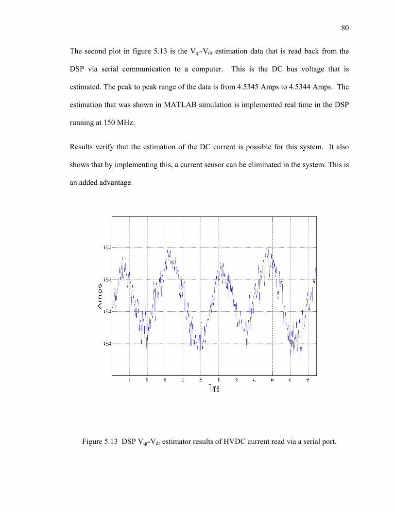
The second plot in figure 5.13 is the Vqr-Vdr estimation data that is read back from the

DSP via serial communication to a computer. This is the DC bus voltage that is

estimated. The peak to peak range of the data is from 4.5345 Amps to 4.5344 Amps. The

estimation that was shown in MATLAB simulation is implemented real time in the DSP

running at 150 MHz.

Results verify that the estimation of the DC current is possible for this system. It also

shows that by implementing this, a current sensor can be eliminated in the system. This is

an added advantage.

Figure 5.13 DSP Vqr-Vdr estimator results of HVDC current read via a serial port.

81

The third plot is the Alpha estimation from the DSP. This information is also read by

using a serial communication to the DSP. The Alpha estimation is used by the control

loop in determination of firing the SCR’s. The range of data is from 83.772 to 83.7708.

Essentially the angle estimation is close to 83 degrees in this instance.

Figure 5.14 DSP Alpha estimator results read back via a serial port.

82

The next plots are from the scope reading of the system voltages and sync signal. It is

very important for this system to sync to the incoming voltage frequency for the SCR’s to

be phase fired. The lab setup was connected to a variable frequency synchronous

generator to produce variable frequency voltage. This represents a wind generator

producing variable frequency power. The plots display this incoming voltage as well as

the DC voltage that is produced by the system. The hardware generated synchronizing

signal is also plotted. This signal is fed to the capture module of the DSP to generate the

Tcap.

The green waveform in the plot is the DC bus voltage, Blue is one phase of the 3 Phase

AC waveform. Magenta is the sync signal. Figure 5.15 shows the synchronizing signal

and DC signal relationship. It is zoomed in to clearly show the synchronizing. In Figure

5.16, the frequency is at 24.23 Hz. In figure 5.17, the synchronizing is at 35.05 Hz.

Figure 5.18, the synchronizing is at 43.15 Hz. Figure 5.19, the synchronizing is at 53.19

Hz. It is seen from the results, the system can synchronizing to a wide frequency range.

You can also observe that the output DC voltage is rising. This is due to the PMSG

voltage rising in relationship to the frequency increase. This experiment purely looks at

the synchronizing capability of the system.

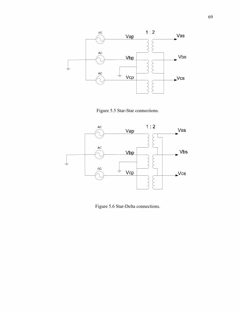
The system only uses the star to star winding to synchronize and has to offset to

account for the star to delta winding firing of the SCR’s. This is accomplished in the

DSP’s SCR firing algorithm. This system was setup to only synchronize between 5Hz

and 80Hz.

83

Figure 5.15 Green DC bus voltage, Blue AC voltage, Magenta synchronizing signal.

Figure 5.16 Green DC bus voltage, Blue AC voltage, Magenta synchronizing signal,

frequency 24.23 Hz.

84

Figure 5.17 Green DC bus voltage, Blue AC voltage, Magenta synchronizing signal,

frequency 35.05 Hz.

Figure 5.18 Green DC bus voltage, Blue AC voltage, Magenta synchronizing signal,

frequency 43.15 Hz.

85

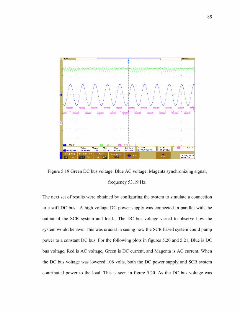
Figure 5.19 Green DC bus voltage, Blue AC voltage, Magenta synchronizing signal,

frequency 53.19 Hz.

The next set of results were obtained by configuring the system to simulate a connection

to a stiff DC bus. A high voltage DC power supply was connected in parallel with the

output of the SCR system and load. The DC bus voltage varied to observe how the

system would behave. This was crucial in seeing how the SCR based system could pump

power to a constant DC bus. For the following plots in figures 5.20 and 5.21, Blue is DC

bus voltage, Red is AC voltage, Green is DC current, and Magenta is AC current. When

the DC bus voltage was lowered 106 volts, both the DC power supply and SCR system

contributed power to the load. This is seen in figure 5.20. As the DC bus voltage was

86

increased to 174 volts, all the power was delivered by the DC power supply and is seen in

figure 5.21. The magenta trace which is the AC current goes to zero.

Figure 5.20 Blue DC bus voltage, Red AC voltage, Green DC current, Magenta AC

current.

87

Figure 5.21 Blue DC bus voltage, Red AC voltage, Green DC current, Magenta AC

current.

The next plot was obtain by changing the lab setup. The system was connected to a

variable frequency synchronous generator and a DC power supply to obtain a full system

performance. The system is given in figure 5.22.

88

Figure 5.22 Lab setup of the complete system connected to a AC generator.

The synchronous generator in figure 5.22 represents a variable frequency wind generator.

The speed of the generator can be varied by using an AC motor drive. In this setup a

Rockwell Automation drive was commanded to change frequency to generate varying

voltage. The SCR conversion system was fed this 3 phase voltage. A DC power supply

was used to maintain a stiff DC bus voltage and a resistor bank was used as a load. The

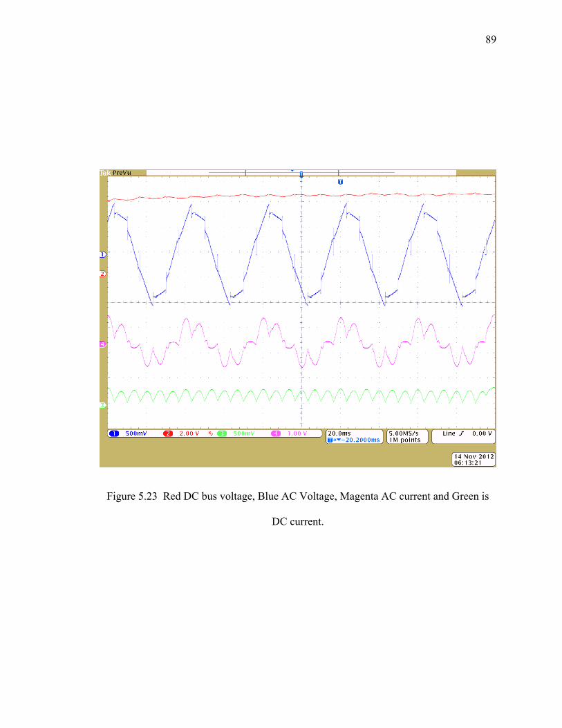
results of this set up are given in figure 5.23. Red is the DC bus voltage, Blue is the AC

Voltage, Magenta is the AC current and Green is the DC current.

89

Figure 5.23 Red DC bus voltage, Blue AC Voltage, Magenta AC current and Green is

DC current.

90

Chapter 6

6.0 Maximum Power Point Tracking (MPPT)

6.1 Wind regions of operation

Modern variable wind generators have three main regions of operation.

These regions are depicted in figure 6.1.

Figure 6.1 Wind Turbine regions of operation.

(Adaptive Torque control of variable speed wind turbine, Kathryn E. Johnson, NREL)

91

Region 1, This is the startup region. The turbine monitors for the wind speed to see if the

turbine can be operated. If it can, it initiates the startup routine. This region does not use

modern controls to improve the capture of wind energy [30] .

Region 2, This is the region that a wind generator should use modern control techniques

to capture the most maximum energy. The maximum energy that can be captured is given

by the Betz limit. The losses in a turbine keeps the generator from reaching this limit.

The idea is to achieve the maximum power extraction. The controls that are available to

maximize are the Yaw angle, generator torque and blade pitch. Since the wind loading in

this region is minimal, it is customary to only control the Yaw angle and generator

torque. Blade pitch angle is left at an optimal angle to capture the maximum energy[47].

Region 3, This is the region that the generator is operating above the rated speed. The

speed of the wind is above the speed that the maximum power can be extracted. The

turbine has to be protected from reaching its maximum mechanical and electrical limits.

Blade pitch control is used to shed the excess wind power. The generator is held at a

constant speed. Yaw angle and generator torque control also can be used to shed the

excess wind power [48].

6.2 Capture of wind energy.

The performance of the wind turbine not only depends on its hardware but also

wind turbine control techniques influence the performance of the wind turbines.

Therefore, the wind turbine control technique can influence the output of the wind

turbine. Fixed speed and variable speed control methods are two traditional control

methods. Variable speed control methods divided into several control methods[45,46].

92

Equation (6.1) show the output power of a wind turbine.

3

2),( windvAcP ρλβ=

(6.1)

λβλ

λβ λ643

2

21

2

5

)(),( cecccccc

+−−=−

(6.2)

1035.0

08.011

32 +

−+

=ββλλ (6.3)

windvRωλ =

(6.4)

Where 3/2.1 mkg=ρ is the air density, A is the area swept by the turbine blades, λ is

the Tip-Speed-Ratio (TSR) given by (6.4), β is the pitch angle, c is the performance

coefficient of the turbine given in (6.2) and ω is the generator angular velocity. c1-c6 are

coefficients that are dependent on the structure of the wind turbine [29].

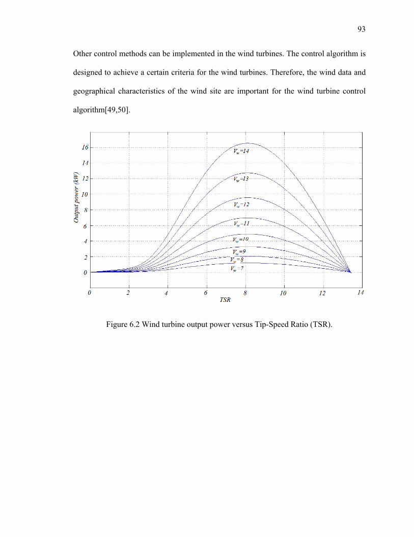
Figure 6.2 shows the power versus TSR. Output power changes with TSR. The

TSR that corresponds to the maximum output power is called optimal TSR. Figure 6.3

shows the output power versus wind turbine speed and compares wind turbine control

methods. One of the lines shows the fixed speed control method and the other one shows

the Maximum Power Extraction (MPE) method (MPE). In MPE algorithm the speed of

the wind turbine is set so that the maximum power can be extracted from the blowing

wind. This speed is called optimal speed. This control method is applicable to variable

speed wind turbines and has better efficiency than the fixed speed method.

93

Other control methods can be implemented in the wind turbines. The control algorithm is

designed to achieve a certain criteria for the wind turbines. Therefore, the wind data and

geographical characteristics of the wind site are important for the wind turbine control

algorithm[49,50].

Figure 6.2 Wind turbine output power versus Tip-Speed Ratio (TSR).

94

Figure 6.3 Wind turbine output power versus rotor speed.

6.3 Wind generator mechanical equations.

The wind generator captures the wind energy using the blades and transfers the power to

the electrical generator. In general, a low speed shaft that is connected to the blades is

fed to a gearbox. The gearbox will increase the speed and is connected to the generator

via a high speed shaft. A generator without a gearbox is referred as a “direct drive”

generator. This type of generator has multiple poles to compensate for the low speed

rotation of the blades. Figure 6.4 is the representation of a geared system.

95

Figure 6.4 Wind Turbine mechanical system of power transfer.

The mechanical equations for the system are as following:

Where, Tm is the mechanical torque produce by the wind. Te is the electrical torque

produced by the generator. B is the frictional coefficient and J is the inertia.

The power generated by the generator is Pe

Using this relationship we can generate a Idc reference related to the ωm reference from

maximum power point tracking as following:

(6.5)

(6.6)

(6.7)

(6.8)

96

The above derivations allows us to control a control system to track the maximum power

point. The inputs to this system are the Wind speed, Radius of the blade (R) and λ

nominal. ω reference compared to the ωm and the error is fed to a PI controller. The

output is divided by HVDC bus voltage and divided by ωe to produce a current

reference to the current control loop. This is given in figure 6.5

Figure 6.5 Configuration of the MPPT Control system.

The output is limited to the I dc reference range of minimum and maximum. “Anti-

winding” PI controller is used.

97

6.4 Simulation results

The simulation results for the figure 6.5 controller is given in Figure 6.6. The first

plot is the reference current corresponding to the MPPT algorithm. The second plot is the

ω reference that is related to the turbine characteristics. In this case, the simulated

turbine has a blade radius of 41 meters, λ nominal of 8.1. The final two plots are the

ωm the turbine speed and wind speed.

Figure 6.6 MPPT Simulation results for changing wind speed.

98

Chapter 7

7.0 Paralleling of wind generators, Fault analysis and Torque pulsations.

7.1 Wind farm operation

The proposed multi-terminal system is given in figure 7.1. The wind farm would have

many generators connected to a common HVDC bus. Each generator would produce

variable voltage and current that would be fed to a step-up transformer to increase the

voltage to the desired DC link voltage. The proposed architecture is scalable to any

number of generators. The HVDC bus would be inverted back to an existing 3 -phase

grid for distribution for utilities.

Figure 7.1 Configuration of the proposed DC distributed PMSG wind farm with multi-

terminal interconnections.

99

Two generators tied to a common DC bus is simulated. The DC bus is held

constant. The wind speed and the pitch angle to the generators are varied to simulate the

varying nature of wind. Each generator is controlled to track for MPPT. The pitch angle

for the generator 1 is change from 0 to 10 at 3 seconds and the same is done for the

generator 2 at 6 seconds independently. The speed of wind is increased to 15 m/s at 7

seconds. In all these cases the control loop compensates for the changes and regulates the

output current in each generator to track MPPT. The simulation results are given in figure

7.3

Figure 7.2 Simulation configuration of Parallel wind generators to a common DC bus.

+

-

DC BUS

Generator 1

Generator 2

100

The first plot is the total current that is produced by the generators. The second plot is

the DC bus, and it is held constant. The third and fourth plots are the generator 1 and 2

pitch angle. The last plot is the wind speed change.

Figure 7.3 Simulation of parallel wind generators connected to a common DC bus.

101

7.2 Faults Analysis

There are two possible faults in the system

• Line faults – generator and inverter side.

• DC Bus faults.

A possible architecture, for a system like this is to only use AC switch gear. In

the event of a Line fault at the generator, the faulty generator can be isolated from the rest

of the system using an AC breaker. If the fault occurs at the inverter side, the inverter

can be isolated from the utility grid using an AC breaker as well as the generators. Same

holds true for DC faults where by using AC breakers the DC bus can be isolated and

protected. Figure 7.4 is the proposed breaker isolation system. Figure 7.5 gives the results

of a 3 phase AC ground fault, the behavior of the current and voltage estimation. It is

seen from the simulation that estimators recover well after ground fault and can track the

voltage and current.

102

Figure 7.4 Configuration of the proposed AC fault isolation with AC breakers.

The first plot is the voltage of the PMSG and a ground fault between 2-3 seconds. The

second plot is the estimation of this voltage. The third is the measured DC current. The

fourth is the estimation of the DC current and the last is the wind speed.

103

Figure . Simulation of Ground Fault on the 3 phase AC generator.

Figure 11. Configuration of the proposed AC

Figure 7.5 Simulation of a ground fault on this system.

Ground Fault

104

7.3 Torque pulsation

A wind generator captures the power in the wind and converts the energy to

mechanical torque. This torque is used to spin the rotor of the generator. The mechanical

equation for the generator is given in equation (7.1). Tm is mechanical torque, Te is

electrical torque, B is the friction coefficient and J is the inertia constant. ωm is the rotor

speed in radians/second. We can see from this equation that any sudden changes in Te

can affect Tm. This is a concern for a generator since torque pulsation can lead to

premature failure of the mechanical components. Figure 7.6 is the simulation of the

torque on the generator[31-40].

(7.1)

The first plot is the electrical torque. The second plot is the wind speed and the last is the

pitch angle. As the pitch angle has a step change the electrical torque of the generator has

a sudden change. This is reflected throughout the system.

105

Figure 7.6 Simulation of torque pulsations.

106

Chapter 8

8.1 DC Power inversion to Grid

The power is collected from all the turbines and transferred to the grid side

inverters via a DC bus. Multiple large size inverters transfer the power to the utility grid.

The grid side inverters adjust the DC voltage of the system and perform grid side

functions such as exporting reactive power. Energy storage components (ultra-capacitor

and batteries) are directly connected to the DC system. They exchange power with the

DC system to perform power ramp rate control, power smoothing, power shifting, and

transient stability control at the wind farm output. The typical capacity factor of a wind

farm is around 30-35%. The additional capacity of the inverter can be used to operate the

energy storage elements when the system is not generating nominal power.

8.2 Selection of the inverter, converter and filter topologies

A three-phase 3-level Neutral Point Clamp (NPC) inverter is chosen as inverter of choice

for this application. The 3-level NPC provides higher quality output voltage and current

waveform and requires a reduced output LCL filter size and cost compared with two level

inverters. Only half of the DC bus voltage has to be switched, which leads to reduced

switching losses and higher efficiency. It also creates less Common Mode (CM) current

at the output to grid. For this application, the switching frequency is around 2-4 kHz. An

LCL filter is designed for the inverter, so the output current profile meets the IEEE 1547

standard [19]-[20]. A passive damping resistor is used to prevent the resonance in the

filter [21].

107

8.3 Control of grid side inverter

Two techniques are employed to control the inverter. 1. Constant DC bus mode of

operation 2. Direct active/reactive power control. In normal operation, when energy

storage is not connected to the DC bus, the active power control is used to regulate the

DC bus voltage. The current control forms the inner loop and the voltage control will

form the outer loop. The current control loop equations are given as below [22]-[24]:

dqddrefi

pd eLiiiSKKv +++⎟

⎠⎞

⎜⎝⎛ +−= ω)(

(8.1)

dqqrefi

pq LiiiSKKv ω−+⎟

⎠⎞

⎜⎝⎛ +−= )(

(8.2)

Vd, Vq, Id and Iq are synchronous reference frame voltage and current. In this case, the

DC bus voltage is controlled using the VSI side DC current. For the voltage control loop

the equation (3) can be derived. Vdc, Idc is DC bus voltage and current respectively.

( )dcrefdci

pLdcdref VVSKKiii −⎟

⎠⎞

⎜⎝⎛ +=−≈ (8.3)

If energy storage is utilized on the DC bus, the active power output can be regulated

independently, considering the state of charge of the storage and the power coming from

the wind farm. In this case, several techniques such as power smoothing, power ramp rate

control, grid frequency support, and/or grid reactive power support can be applied.

108

8.3 Frequency droop and voltage droop control

The proposed MVDC system can provide frequency and voltage support to the grid.

Typically, renewable energy systems ride on grid frequency and voltage and do not

provide significant ancillary services. However, as renewable installed capacity is rising

to become a significant part of the total grid capacity, it must participate in grid support

functions. There are several mechanisms including generator governor, automatic gain

control and load shedding. The proposed system can provide an alternative mechanism,

which can be applied faster than conventional methods. The proposed MVDC system

with ultra-capacitors and battery backup with DC/DC converter can allow the VSI to

support frequency droop for a short duration before automation generation control take

appropriate action. Similarly it can support the system to keep the AC voltage within

range by regulating the reactive power.

The main advantages of the proposed MVDC system are active and reactive power rate

control, frequency droop control and voltage droop control.

The proposed complete system from the generator to the inverter that ties to the grid is

given in figure 8.1. The controls for both the PMSG and the Inverter are presented.

109

Figure 8.1 Wind energy conversion system with energy storage.

110

Chapter 9

9.0 Conclusion

In chapter 1, the importance that wind energy plays in the future energy generation is

discussed. The current wind generator technology, the difference between a DFIG and

PMSG generators are looked at. The problem and the solution that this work is centered

around is stated and discussed. How wind generators connected to a HVDC/MVDC bus,

tied to a grid via inverters are presented as a possible system.

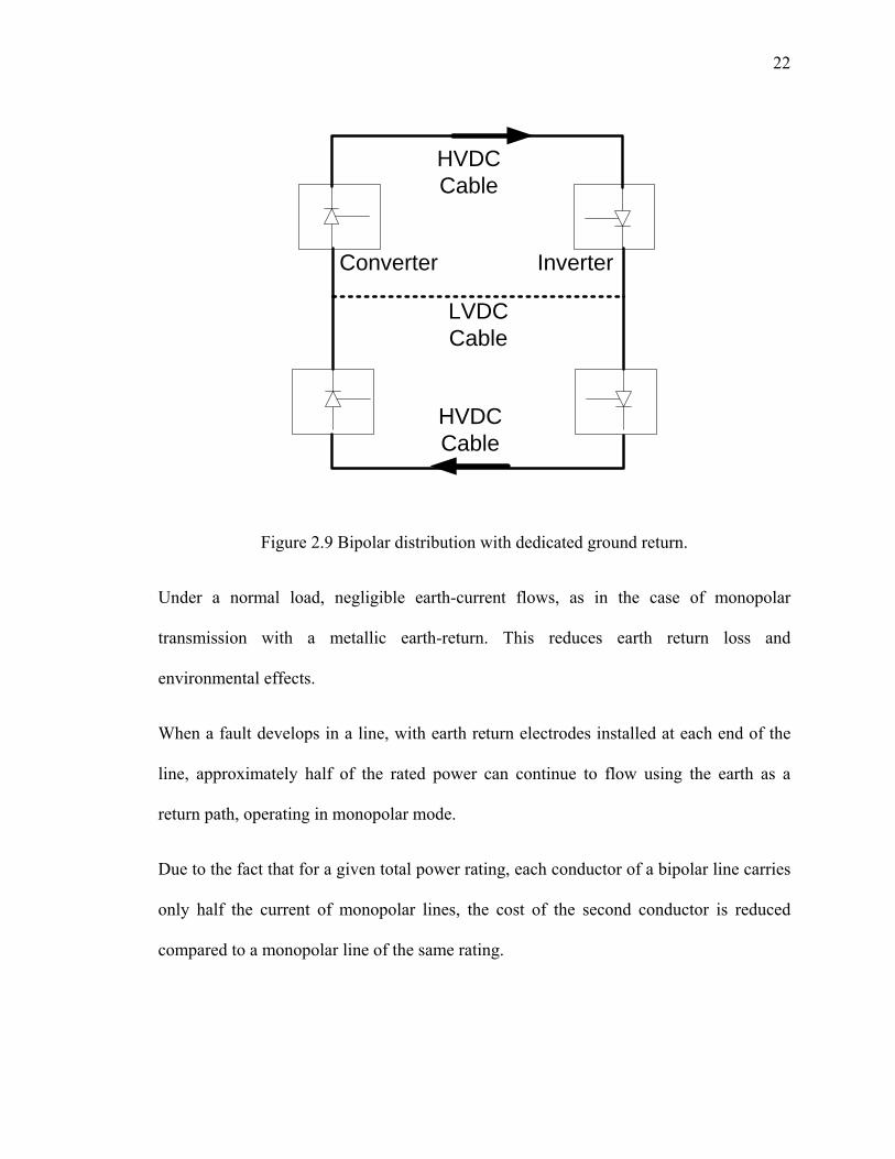
Chapter 2 is dedicated to studying the HVDC/MVDC distribution. The different

configuration of the HVDC distribution systems are presented. The advantages and

disadvantages of the AC and DC distribution are evaluated. The converter used to convert

AC power to DC power is looked at. Finally faults and redundancy in a DC distribution is

analyzed.

Chapter 3 details this possible solution. The use of SCR as a power semiconductor

device is presented. The system is modeled and simulated in MATLAB® and Simulink®.

The parameter of a direct drive 1.5 MW generator is used in the simulation. The results of

the simulation is discussed.

Chapter 4 focuses on the control system for the PMSG and 12 pulse SCR’s. Three

estimator are developed to aid in controlling this system. The first estimator estimates

the PMSG generator voltages. The second estimator estimates the DC bus current and the

third estimates the Alpha angle for firing the SCR’s.

111

Chapter 5 is the Lab setup. The power section where the SCR’s reside and how they are

connected to the star and delta transformers are shown. A Texas instrument DSP is used

to run this system in real time. The program flow as well as SCR gate and signal

connection are illustrated. The system is run and data is gathered. The results are

discussed and compared to the simulated results.

Chapter 6, the MPPT algorithm is developed. The wind turbine regions of operation and

the Betz limits are discussed. Turbine energy capture and the necessary equations

describing the mechanical system are presented. MPPT algorithm is simulated in

MATLAB® and Simulink®.

Chapter 7 looks at how this system can be implemented in a wind farm. Two wind

generators independently running and tied to a common DC bus is simulated. The results

are presented. This proves the proposed system is viable for a wind farm. Another

concern is how to protect such a system from faults. A possible fault isolation system is

presented and simulated. Finally the torque that is generated by this system is studies as

the power is varied.

Chapter 8, the final chapter looks at how the DC bus power is converted to the utility grid

via inverters. The control of the inverter and interaction with the grid are stated. The

inverters hold the DC bus voltage constant, enabling the wind generators to transfer

power independently. This total generation, distribution and grid connection is presented

in this chapter.

112

The following was accomplished in this work:

• Controls of a 12-pulse SCRs system to connect PMSG wind turbines to a HVDC

bus was proposed.

• Three estimators are designed to estimate the generator terminal voltage, output

DC current and firing angle in order to control the SCRs.

• The proposed system was fully simulated using Matlab/ Simulink.

• An experimental hardware setup was built to verify the operation of the system.

This setup was connected to a synchronous generator and results are presented.

• Parallel wind generator setup was simulated. The results verifies that the

proposed system will work for a wind farm.

• A fault isolation system was proposed and simulated , which shows how the

system can tolerate faults and recover.

• Torque ripple on the generator was simulated to see the SCR’s switching effecte

on the generator.

• This setup was verified as a robust and a low cost method of implementing PMSG

for HVDC distribution.

The following is proposed as future work:

• Explore different control methods for controlling the SCR’s.

• Investigate reducing torque pulsations of the PMSG.

113

• Investigate using the proposed power conversion method for DFIG turbines.

• Explore options for communication/control between PMSG, circuit protection and

grid-tied inverters.

• Investigate the best possible configuration for DC storage/connection to the

HVDC/MVDC bus.

• Study the filtering needed to improve the DC bus voltage at the PMSG

connections.

114

References

[1] M. Fatu, C. Lascu, G. Andreescu, R. Teodorescu, F. Blaabjerg, I. Boldea, “Voltage Sags Ride-Through of Motion Sensor less Controlled PMSG for Wind Turbines,” in Proc. 42nd IEEE IAS Annual Meeting Industry Applications Conference, New Orleans, LA 2007, pp. 171 – 178,.

[2] Abedini, G. Mandic, and A. Nasiri, “Wind power smoothing using rotor inertia aimed at reducing grid susceptibility,” Int. J. of Power Electronics, vol. 1, no. 2, pp. 227 - 247, 2008

[3] H. Peterson and P. Krause, Jr., “A Direct-and Quadrature-Axis Representation of a Parallel AC and DC Power System,” IEEE Transactions on Power Apparatus and Systems, vol. PAS-85, no.3, pp. 210 – 225, March, 1966.

[4] L. Wang, K. Wang, W. Lee and Z. Chen, “Power Flow Control and stability Enhancement of Four Parallel Operated offshore Wind Farms Using a Line Commuted HVDC Link,” IEEE Transaction on Power Delivery, vol. 25, no. 2, pp. 1190-1202, April 2010.

[5] Kun Han and Guo-zhu Chen, “A Novel Control Strategy of Wind Turbine MPPT Implementation for Direct-Drive PMSG Wind Generation Imitation Platform,” IEEE 6th International Power Electronics and Motion Control Conference, May 2009, pp. 2255 – 2259, Wuhan, China.

[6] M. Eduardo, M. DJesus, D. Martin, S. Arnaltes and E. Castronuovo, “Optima Operation of Offshore Wind Farms With Line-Commutated HVDC Link Connection,” IEEE transactions on energy conversion, vol. 25 no. 2, June 2010.

[7] Y. Weizheng, K. Woo, Z. Ruijie, G. Wei and W. Yue, “Analyze of Current Control Strategy based on Vector Control for Permanent-Magnet Synchronous Generator in Wind Power System,” IEEE Power Electronics and Motion Control Conference, 2009, pp. 2209 – 2212.

[8] M. Li, K. Smedley, “One-Cycle Control of PMSG for Wind Power Generation,” IEEE Power Electronics and Machines in Wind Applications, 2009.

[9] M. Chinchilla, S. Arnaltes and J. Burgos, “Control of Permanent-Magnet Generators Applies to Variable-Speed Wind Energy System Connected to the Grid,” IEEE transactions on energy conversion, vol. 21, no,1,March 2006

[10] N.M Kirby,L. Xu, M. Luckett, and W. Siepman, “HVDC Transmission for Large Wind Farms”, IEEE Power Engineering Journal, June 2002.

115

[11] J.B Ekanayake, L. Holdsworth, X.G. Wu and N.Jenkins, “Dynamic Modeling of Doubly fed Induction Generator Wind Turbines”, IEEE Transactions on Power Systems”, VOL1, pp.803-809, May2009

[12] Chan-Ki Kim, Vijaya K.Sood, Gil-Soon Jang, Seong-Joo Lim, Seoak-Jin Lee, “HVDC Transmission: Power Conversion Application in Power Systems”

[13] Vijaya K.Sood, “HVDC and FACTS Controllers: Applications of Static Converters in Power Systems”

[14] Ned Mohan, Tore M. Undeland, William P. Robbins “Power electronics: converters, applications, and design - Volume 1”

[15] P. Cartwright and L. Xu, “The Integration of large scale wind power generation into transmission network using power electronics” CIGRE General Session, Paris 2004

[16] S. Bozhko,R. Blasko-Gimenez,R. Li,J. Clare,G. Asher “Control of Offshore DFIG-based Wind Farm Grid with Line-Commutated HVDC Connection”

[17] Xie Lei,Xie Da,Zhang Yanchi “Offshore wind farm with dispersed wind turbines control and HVDC grid-connected control”

[18] D.Jovcic,J.Milanovic”Offshore wind farm Based on Variable Frequency Mini-Grids with Multiterminal DC Interconnections.

[19] Y. Patel, D. Pixler, A. Nasiri, “Analysis and design of TRAP and LCL filters for active switching converters,” IEEE industrial electronics international symposium (ISIE), pp 638-643, 2010

[20] M. Liserre, F. Blaabjerg, and S. Hansen. "Design and Control of an LCLfilter based Three-phase Active Rectifier," Conf Rec. of 36th IAS Ann. Meeting, Chicago, 2001, pp. 297-307.

[21] M. Loserre, A. Dell’Aquila, F. Blaabjerg, “Genetic algorithm-based design of the active damping for an LCL filter three phase active rectifier,” IEEE Trans. Power electronics., vol. 19, no. 1, pp. 76–86, Jan. 2004.

[22] V. Blasko and V. Kaura, “A novel control to actively damp resonance in input LC filter of a three-phase voltage source converter,” IEEE Trans.Ind. Appl., vol. 33, no. 2, pp. 542–550, Mar./Apl. 1997.

[23] Y Lang; X Zhang; D Xu;, S. Hadianamrei; H Ma, “Nonlinear Feedforward Control of Three-phase Voltage Source Converter,” IEEE Industrial Electronics., vol. 2 pp. 1134-1137, Jul 2006

116

[24] R. M. Tallam, R. Naik, M. L. Gasperi, T.A. Nondahl, Hai Hui Lu, Yin Qiang, “Practical issues in the design for AC drives with reduced DC link capacitor,” Conf Rec. of 38th IAS Ann. Meeting, vol. 3, pp. 1538-1545, 2003

[25] T. Ackermann, “Wind Power in Power Systems”, John Wiley & Sons, 2005.

[26] L. H. Hansen, L. Helle, F. Blaabjerg, E. Ritchie, S. Munk-Nielsen, H. Bindner, P. Sørensen and B. Bak-Jensen, “Conceptual survey of Generators and Power Electronics for Wind Turbines”, 2001.

[27] Johnson, Gary L. “Wind energy systems”, Prentice-Hall, inc 1985.

[28] High Voltage Proven Technology -SIEMENS

[29] http://www.mathworks.com/products/simpower/blocklist.html

[30] Adaptive Torque control of variable speed wind turbine, Kathryn E.

Johnson, NREL

[31] G. Mandic, A. Nasiri, E. Muljadi, and F. Oyague, “Active torque control for gearbox load reduction in a variable speed wind turbine,” accepted of publication in IEEE Trans. Ind. Appl., 2012

[32] Y. Hori, H. Iseki, and K. Sugiura, “Basic consideration of vibration suppression and disturbance rejection control of multi-inertia system using SFLAC (state feedback and load acceleration control),” IEEE Trans. Ind. Appl., vol. 30, no. 4, pp. 889–896, Jul./Aug. 1994.

[33] M. Cychowski, K. Szabat, and T. Orlowska-Kowalska, “Constrained model predictive control of the drive system with mechanical elasticity,” IEEE Trans. Ind. Electron., vol. 56, no. 6, pp. 1963–1973, Jun. 2009.

[34] K. Szabat and T. Orlowska-Kowalska, “Vibration suppression in a two-mass drive system using PI-speed controller and additional feedbacks—Comparative study,” IEEE Trans. Ind. Electron., vol. 54, no. 2, pp. 1193–1206, Apr. 2007.

117

[35] A. Dixit and S. Suryanarayanan, “Towards Pitch-Scheduled Drive Train Damping in Variable Speed, Horizontal-Axis Large Wind Turbines,” in Proc. 44th CDC-ECC, Seville, Spain, Dec. 12-15, 2005.

[36] S.H. Kia, H. Henao, and G.-A Capolino, “Torsional Vibration Effects on Induction Machine Current and Torque Signatures in Gearbox-Based Electromechanical System,” IEEE Trans. Ind. Electron., vol. 56, no. 11, pp. 4689-4699, Nov. 2009.

[37] H. Geng, D. Xu, B. Wu, and G. Yang, "Active Damping for PMSG based WECS With DC-Link Current Estimation," IEEE Trans. Ind. Electron., vol.58, pp. 1110-1119, Apr. 2011.

[38] M. Molinas, J. A. Suul, and T. Undeland, “Torque transient alleviation in fixed speed wind generators by indirect torque control with STATCOM,” in Proc. 13th EPE-PEMC, Poznan, Poland, Sep. 1–3, 2008, pp. 2318–2324.

[39] T. Zoller, T. Leibfried, and A.M. Miri, “Application of Power Electronics for Damping of Torsional Vibrations,” in Proc. 7th PEDS, Bangkok, Thailand, Nov. 27-30, 2007.

[40] R. Muszynski and J. Deskur, “Damping of Torsional Vibrations in High-

Dynamic Industrial Drives,” IEEE Trans. Ind. Electron., vol. 57, pp. 544-552, Feb. 2010.

[41] E. A. Bossanyi, “The Design of Closed Loop Controllers for Wind Turbines,” Wind Energy, vol. 3, pp. 149-163, 2000.

[42] H. Polinder, F. F. A. van der Pijl, G. J. de Vilder, and P. J. Tavner, “Comparison of Direct-Drive and Geared Generator Concepts for Wind Turbines,” IEEE Trans. Energy. Convers., vol. 21, pp. 725-733, Sep. 2006.

[43] I. Boldea Variable Speed Generators, CRC Press, 2005

118

[44] J. L. Rodriguez-Amenedo, S. Arnalte, and J.C. Burgos, “Automatic generation control of a wind farm with variable speed wind turbines,” IEEE Trans. Energy Convers., vol.17, no.2, pp.279-284, Jun. 2002.

[45] Q.Q. Wang, “Maximum wind energy extraction strategies using power electronic converters”, Ph.D. Dissertation, University of New Brunswick, 1996

[46] E.Koutroulis, and K.Kalaitzakis, “Design of a Maximum Power Tracking System for Wind-Energy-Conversion Applications,” IEEE Trans. Ind. Electron., vol. 53, no. 2, pp. 486-494, Apr. 2006.

[47] E. Muljadi and C.P. Butterfield, "Pitch-controlled variable-speed wind turbine generation," IEEE Trans. Ind. Appl., vol.37, no.1, pp.240-246, Jan/Feb 2001.

[48] O. Anaya-Lara, N. Jenkins, J. Ekanayake, P. Cartwright, M Hughes, Wind Energy Generation : Modeling and Control. John Wiley & Sons, 2009.

[49] Y. Chen, P. Pillay, and A. Khan, “PM wind generator topologies,” IEEE Trans. Ind. Appl., vol. 41, no. 6, pp. 1619–1626, Nov./Dec. 2005.

[50] G. Mandic, and A. Nasiri, “Modeling and simulation of a wind turbine system with ultracapacitors for short-term power smoothing,” IEEE ISIE 2010, Bari, Italy, July 2010.

119

CURRICULUM VITAE

RAVI NANAYAKKARA

2520 Rebecca DR., Racine, WI 53402 (262)-752-4854

ravin@ieee.org

EDUCATION:

Doctor of Philosophy – Electrical Engineering (Power Electronics)

University of Wisconsin Milwaukee, Milwaukee, Wisconsin December 2012

Master of Science in Electrical and Computer Engineering

Marquette University, Milwaukee, Wisconsin December 2001

Bachelor of Science in Electrical Engineering

University of Wisconsin Milwaukee, Milwaukee, Wisconsin May, 1997 commencement Honors

SUMMARY:

A highly motivated and analytical professional with 17+ years of work experience at a leading Industrial Automation and Controls Corporation. Hardware design, simulation and new product development experience coupled with strong interpersonal communication and project management skills.

120

PROFESSIONAL OVERVIEW:

ROCKWELL AUTOMATION-ALLEN BRADLEY

Milwaukee,Wisconsin

Project Engineer Hardware February,2005 to Present

Responsible for overseeing a project from inception to finish. Overall responsibility for setting the project technical direction. Responsible for working with cross-functional teams to establish customer requirements for new products.

• Design of next generation 690/480 volt three phase motor controller. • MATLAB® and Simulink®. modeling. • Power electronics/Digital/communication hardware design. Includes High speed

SCR gate drive design, DSP, Input/output circuitry, Voltage and Current controller design as well as Power supply design.

Senior Hardware Design Engineer April,2001 to February ,2005

Team member of a new product development team responsible for designing the next generation HMI products.

• Project lead responsibility for design and development of a new display platform. This is the largest HMI display platform undertaken by the business with the largest estimated profit margins.

• In depth knowledge of display interfacing technology. Implemented DVI /LVDS interface in driving large-scale displays to reduce EMI. This in turn produced cost savings of half a million a year and ease of manufacturing by using board to board interconnects.

• Responsible for the new design of scalable inverter architecture for driving CCFL backlights for flat panel TFT displays of various sizes. Exceeded the cost; size and performance goals set in the design specification.

• Design of low power white LED drivers for battery operated hand held displays. • Design of battery charging circuit for Lithium Ion. Embedded system

development with 32 bit microprocessor, 8 bit micro programming experience, SDRAM, Flash, DDR, USB, CPLD, Ethernet 10/100 implementation experience.

• Familiarity with safety standards and EMC regulations world wide. Worked with UL representatives in obtaining agency approvals for designs. Designed products for CE, CUL, UL, Demco, Ctic and other industrial safety standards.

• Responsible for design specifications and cross-functional integration with mechanical, test engineering and manufacturing teams. Overall responsibility for all display heads design and pilot production.

121

Hardware Design Engineer July, 1997 to April, 2001

Responsible for overall power supply architecture for supporting the hardware platform of the next generation operator interface terminals.

• Design of distributed DC/DC power supplies for an embedded platform. Special emphasis on low voltage and high current core operation of microprocessors. High efficiency (85%-90%) DC power supply design using synchronous rectification. Low EMI power supplies using out of phase switching regulators.

• Design of AC/DC switch mode power supplies for industrial environment. • Analysis of analog designs with Accusim simulation, Saber simulation , Mathcad

and Matlab tools. Schematic capture using Mentor graphics. • Worked with mechanical teams in thermal management and packaging of

products. Component de-rating and analysis for meantime failure. Implemented accelerated life test for power supply testing.

Engineering Intern June,1995 to July,1997

Designed systems for testing Man Machine Interface (MMI) with Allen-Bradley Programmable Logic controllers.

Worked with DH+, DH485, DF1, RIO, Controllnet and DeviceNet protocols. Design and development of table driven test software using Visual Basic allowing faster functional evaluation of the development software.

PROFESSIONAL & ACADEMIC SKILLS

• Two patents have been filed as well as numerous innovation awards. • Knowledge of modern control theory including state space control and non-linear

adaptive control. • Ability to analyze stability of a control loop, Optimize a control loop for desired

response. • Experience in designing power inductors and transformers • IEEE Member