SEARCH FOR THE STANDARD MODEL HIGGS BOSON IN LEPTONS PLUS JETS FINAL STATES By Huong Thi Nguyen A DISSERTATION Presented to the Graduate Faculty of the University of Virginia in Candidacy for the Degree of Doctor of Philosophy Department of Physics Unversity of Virginia January, 2014
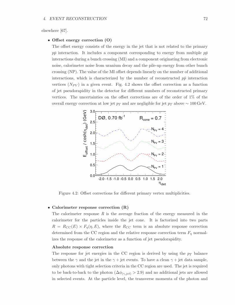
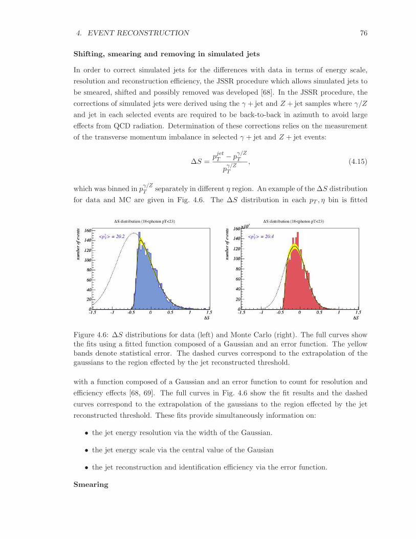
Transcript
SEARCH FOR THE STANDARD MODEL HIGGS BOSON
IN LEPTONS PLUS JETS FINAL STATES
By
Huong Thi Nguyen
A DISSERTATION
Presented to the Graduate Faculty
of the University of Virginia in Candidacy for the Degree of
Doctor of Philosophy
Department of Physics
Unversity of Virginia
January, 2014
i
ACKNOWLEDGMENTS
First and foremost, I gratefully acknowledge the continual guidance and support of my
adviser, Professor Bob Hirosky. His dedication to research and pursuit of physics have been
an invaluable source of inspiration and encouragement to us, his students.
I had the privilege of being on the teams of the ZHllbb and LNUJJ analysis groups in the D0
Collaboration and I would like to deeply thank all members of these two research groups. I
will always remember the stimulating discussions and scientific atmosphere we shared with
one another over the last four years.
Finally, I could not have achieved this without the support, encouragement and love from
my friends and family, particularly my children, Chau and Minh.
Huong Nguyen
Charlottesville, Virginia
January, 2014
CONTENTS ii
Contents
1 Introduction 1
2 The Standard Model and Higgs Physics 4
2.1 The Standard Model of Particle Physics . . . . . . . . . . . . . . . . . . . . 4
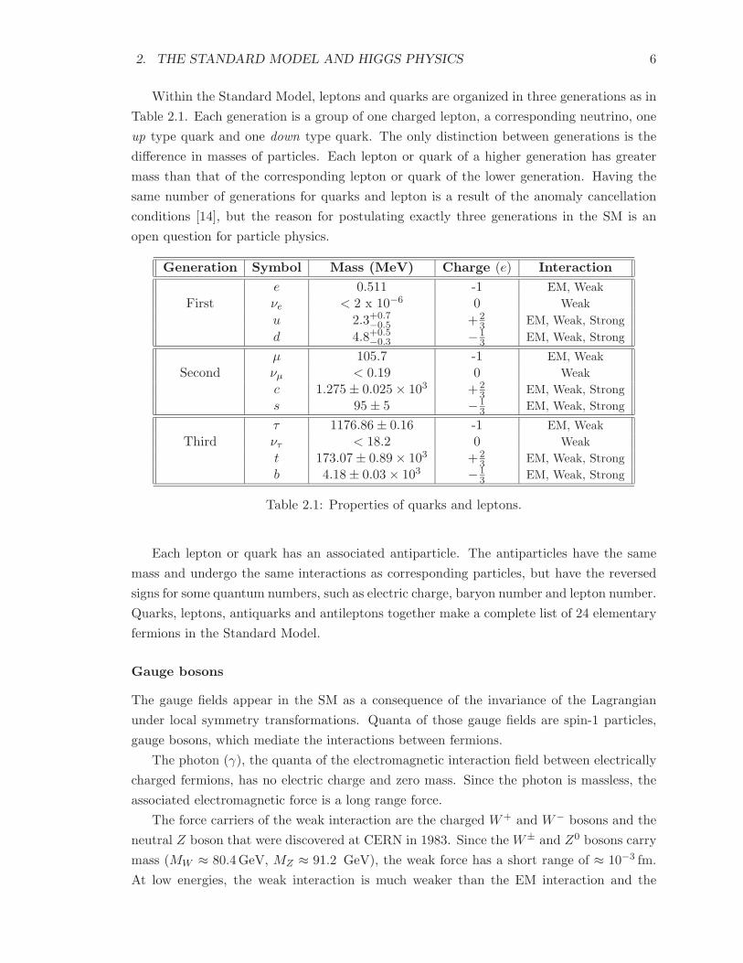
The Higgs doublet of complex scalar fields introduced in the Higgs mechanism is a singlet
of SU(3)C, doublet of SU(2)L and carries hypercharge Y = +1/2. It can be expressed as a
scalar representation of the gauge symmetry group:
φ(1, 2)+1. (2.66)
Explicitly adding the lepton or quark mass terms (−mψψ) to the Lagrangian of the fermion
system in Eqn. (2.22) violates the gauge theory. To retain the gauge invariance, the fermion
mass needs to be introduced into the SM model through the Yukawa interaction between
the Higgs field and the fermions fields. The contribution to the Lagrangian of the coupling
for three fermion families to the Higgs field is taken to be:
LYukawa = LleptonYukawa + Lquark
Yukawa (2.67)
LleptonsYukawa = −Y e
ijLILiφE
IRj − Y e⋆
ij EIRjφL
ILi
LquarksYukawa = −Y d
ijQILiφD
IRj − Y u
ijQILiφU
IRj − Y d⋆
ij DIRjφQ
ILi − Y u⋆
ij UIRjφQ
ILi
where Y eij , Y
dij and Y u
ij are arbitrary complex matrixes, and the conjugate of the Higgs field
φ is constructed as :
φ(1, 2)−1 = −iτ2φ⋆ =
(−φ0
φ−
)
(2.68)
Gathering all ingredients together, we have the Standard Model Lagrangian LSM , which is
consistent with the gauge symmetry in Eqn. (2.64) and particle content shown in Eqns. (2.65)
and (2.66), written as:
LSM = Lkinetic + LHiggs,+LYukawa, (2.69)
2. THE STANDARD MODEL AND HIGGS PHYSICS 21
where LYukawa (2.67) describes the Yukawa coupling and LHiggs represents the scalar self
interaction:
LHiggs = −µ2φ†φ− λ(φ†φ)2. (2.70)
The Lkinetic includes kinematic terms of all the fields:
Lkinetic = Lleptonkinetic + Lquark
kinetic + Lgaugekinetic + LHiggs
kinetic
Lleptonkinetic = LI
Liγµ(i∂µ − gW aµT a − g′
2BµY )LI
Li + EIRiγµ(i∂µ − g′
2BµY )EI
Ri
Lquarkkinetic = QI
Liγµ(i∂µ − gsGbµLb − gW aµT a − g′
2BµY )QI
Li
+U IRiγµ(i∂µ − gsG
bµLb − g′
2BµY )U I
Ri
+DIRiγµ(i∂µ − gsG
bµLb − g′
2BµY )DI
Ri
LHiggskinetic =
∣∣∣(∂µ + igW a
µTa + i
g′
2BµY )φ
∣∣∣
2
LGaugekinetic = −1
4BµνB
µν − 1
4W a
µνWaµν − 1
4Gb
µνGbµν (2.71)
Expanding the SM Lagrangian LSM around the vacuum states of the Higgs field is equivalent
to substituting φ(1, 2)+1 and φ(1, 2)−1 in Eqn. (2.69) with:
φ =
(−φ+
φ0
)
−→(
0v+h(x)√
2
)
, φ =
(−φ0
φ−
)
−→( v+h(x)√
2
0
)
(2.72)
Under spontaneous symmetry breaking, the Standard Model symmetry group GSM breaks
down as:
SU(3)C ⊗ SU(2)L ⊗ U(1)Y → SU(3)C ⊗ U(1)EM (2.73)
The gluons and the photons associated with generators of the unbroken parts, SU(3)C and
U(1)EM , remain massless, while W± and Z weak bosons acquire a masses as shown in
Eqn. (2.59).
Decomposing the SU(2)L lepton and quark doublets into their components as:
LILi(1, 2)−1 =
(νI
eL
eIL
)
,
(νI
µL
µIL
)
,
(νI
τL
τ IL
)
; QILi =
(U I
Li
DILi
)
(2.74)
and applying the substitution Eqn. (2.72) to Eqn. (2.67), we obtain the Yukawa interaction
terms of the SM Lagrangian expressed in terms of the vacuum expectation value and of the
neutral scalar Higgs field h(x) as:
LleptonsYukawa = −v + h√
2(eIL, µ
IL, τ
IL) Ye (eIR, µ
IR, τ
IR)T + hermitian conjugate (2.75)
2. THE STANDARD MODEL AND HIGGS PHYSICS 22
LquarksYukawa = −v + h√
2(DI
L1, DIL2, D
IL3) Yd (DI
R1, DIR2, D
IR3)
T
−v + h√2
(U IL1, U
IL2, U
IL3)Y
u(U IR1, U
IR2, U
IR3)
T + hermitian conjugate(2.76)
Upon spontaneous symmetry breaking, the Yukawa interactions give rise to the mass
terms of leptons and quarks:
LleptonsMass = − v√
2(eIL, µ
IL, τ
IL) Ye (eIR, µ
IR, τ
IR)T + hermitian conjugate (2.77)
LquarksYukawa = − v√
2(DI
L1, DIL2, D
IL3) Yd (DI
Rj , DIRj , D
IRj)
T
− v√2(U I
L1, UIL2, U
IL3)Y
u(U IR1, U
IR2, U
IR3)
T + hermitian conjugate
(2.78)
Each matrix of Y e, Y u, Y d can be diagonalized with a set of two chosen 3 × 3 unitary
matrixes:
Y ediag = Ve
L Ye Ve†R , Y u
diag = VuL Yu Vu†
R , Y ddiag = Vd
L Yd Vd†R (2.79)
and the mass eigenstates of quarks and leptons are defined as:
ULi = (V uL )ijU
ILj
URi = (V uR )ijU
IRj
DLi = (V dL )ijD
ILj
DRi = (V dR)ijD
IRj
(eL, µL, τL)T = V eL(eIL, µ
IL, τ
IL)T
(eR, µR, τR)T = V eR (eIR, µ
IR, τ
IR)T (2.80)
Then, from (2.77), (2.79) and (2.80), the masses of the leptons are given by:
me =fev√
2, mµ =
fµv√2, mτ =
fτv√2, (2.81)
where the diagonal elements of Y ediag, fe, fµ, and fτ , are dimensionless Yukawa coupling
constants.
Similarly, the masses of the six different flavor quarks are obtained from Eqns. (2.78), (2.79)
and (2.80):
mu =fuv√
2, mc =
fcv√2, mt =
ftv√2
md =fdv√
2, ms =
fsv√2, mb =
fbv√2, (2.82)
2. THE STANDARD MODEL AND HIGGS PHYSICS 23
It can be seen from Eqn. (2.75) and Eqn. (2.76) that introducing masses for charged leptons
and quarks through the Yukawa interaction also gives a rise to the interaction between those
fermions and the Higgs boson with coupling strength being proportional to the fermion mass:
f =
√2mf
v(2.83)
Couplings of the Higgs boson to itself as well as to fermions and gauge bosons are charac-
terized by the Feynman diagrams in Fig. 2.2.
(a) (b) (c)
(d) (e) (f)
Figure 2.2: Feynman rules for the SM Higgs Boson
2.2 The Standard Model Higgs Physics
2.2.1 Theoretical Constraints on the Higgs Boson Mass
The Higgs mechanism in the Standard Model requires the presence of the Higgs boson as a
direct physical manifestation of the origin of the mass. The Higgs boson appears to be an
electrically neutral particle which has mass depending on two parameters, MH =√
2v2λ.
The parameter v related to vacuum expectation value of the Higgs field is experimentally
determined by the mass of the weak gauge bosons. So far, there has been no way to calculate
the Higgs boson self-coupling constant λ, which characterizes the scalar potential, without
having experimental knowledge about the SM Higgs spectrum itself. Therefore, the mass of
the Higgs boson remains as unspecified parameter in the SM theory. However, theoretical
studies to determine constraints on the mass of the Higgs boson from considering triviality
and vacuum stability lead to the upper and lower bounds on the mass, respectively [18].
2. THE STANDARD MODEL AND HIGGS PHYSICS 24
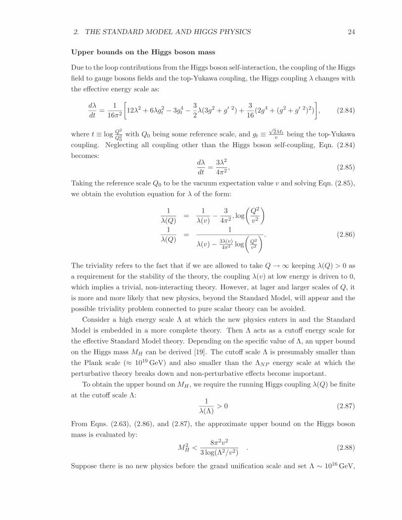
Upper bounds on the Higgs boson mass
Due to the loop contributions from the Higgs boson self-interaction, the coupling of the Higgs
field to gauge bosons fields and the top-Yukawa coupling, the Higgs coupling λ changes with
the effective energy scale as:
dλ
dt=
1
16π2
[
12λ2 + 6λg2t − 3g4
t − 3
2λ(3g2 + g′ 2) +
3
16(2g4 + (g2 + g′ 2)2)
]
, (2.84)
where t ≡ log Q2
Q20
with Q0 being some reference scale, and gt ≡√
2Mt
v being the top-Yukawa
coupling. Neglecting all coupling other than the Higgs boson self-coupling, Eqn. (2.84)
becomes:dλ
dt=
3λ2
4π2, (2.85)
Taking the reference scale Q0 to be the vacuum expectation value v and solving Eqn. (2.85),
we obtain the evolution equation for λ of the form:
1
λ(Q)=
1
λ(v)− 3
4π2, log
(Q2
v2
)
1
λ(Q)=
1
λ(v) − 3λ(v)4π2 log
(
Q2
v2
) . (2.86)
The triviality refers to the fact that if we are allowed to take Q→ ∞ keeping λ(Q) > 0 as
a requirement for the stability of the theory, the coupling λ(v) at low energy is driven to 0,
which implies a trivial, non-interacting theory. However, at lager and larger scales of Q, it
is more and more likely that new physics, beyond the Standard Model, will appear and the
possible triviality problem connected to pure scalar theory can be avoided.
Consider a high energy scale Λ at which the new physics enters in and the Standard
Model is embedded in a more complete theory. Then Λ acts as a cutoff energy scale for
the effective Standard Model theory. Depending on the specific value of Λ, an upper bound
on the Higgs mass MH can be derived [19]. The cutoff scale Λ is presumably smaller than
the Plank scale (≈ 1019 GeV) and also smaller than the ΛNP energy scale at which the
perturbative theory breaks down and non-perturbative effects become important.
To obtain the upper bound on MH , we require the running Higgs coupling λ(Q) be finite
at the cutoff scale Λ:1
λ(Λ)> 0 (2.87)
From Eqns. (2.63), (2.86), and (2.87), the approximate upper bound on the Higgs boson
mass is evaluated by:
M2H <
8π2v2
3 log(Λ2/v2). (2.88)
Suppose there is no new physics before the grand unification scale and set Λ ∼ 1016 GeV,
2. THE STANDARD MODEL AND HIGGS PHYSICS 25
the upper bound on the Higgs boson mass is then estimated as:
MH < 160 GeV. (2.89)
It can be seen from Eqn. (2.87) that as the cutoff scale Λ becomes smaller, the constraint
on the Higgs mass upper bound becomes progressively loose. For example, with Λ ∼ 3 TeV,
the upper bound is roughly 600 GeV.
Considering the contribution of the top quark and gauge bosons to the evolution equation
for λ, but just focusing on the case of a heavy Higgs boson, which corresponds to λ >
gt, g, g′, the equation of running λ (Eqn. (2.84)) is simplified as:
dλ
dt∼ λ
16π2
[
12λ+ 6g2t − 3
2(3g2 + g′ 2)
]
. (2.90)
Following a similar analysis applied for the pure scalar field theory and requiring the running
coupling λ(Λ) to be finite up to the scale Λ, a more stringent upper limit on the Higgs
boson mass is obtained as a function of top quark mass Mt. The upper curve in Fig. 2.3
shows the upper bound on the Higgs mass as a function of the cutoff scale Λ [19]. The
numerical value for the bound is calculated with considering the evolution of the gauge
coupling constants and top-Yukawa coupling. The upper filled area indicates the sum of
theoretical uncertainties in the MH upper bound when keeping top quark mass fixed at
Mt = 175 GeV. The cross-hatched area shows the additional uncertainty when varying Mt
from 150 to 200 GeV.
Lower bound on the Higgs boson mass
The lower bound on the Higgs boson mass is derived from requiring the spontaneous
symmetry-breaking minimum to be an absolute minimum of the effective Higgs potential
up to some cutoff scale Λ. This requirement, referred to as vacuum stability, is essentially
equivalent to requiring the Higgs running coupling λ to remain positive at all scales up to
a cutoff point Λ.
At the limit where the Higgs boson mass is small (corresponding to small λ), the evolu-
tion equation for λ in Eqn. (2.84) becomes:
dλ
dt=
1
16π2
[
−3g4t +
3
16(2g4 + (g2 + g′ 2)2)
]
(2.91)
The solution to Eqn. (2.91) at scale Λ is written as:
λ(Λ) = λ(v) +1
16π2
[
−3g4t +
3
16(2g4 + (g2 + g′ 2)2)
]
log
(Λ2
v2
)
(2.92)
Imposing the requirement of vacuum stability (λ(Λ) > 0) on Eqn. (2.92) and using the
relation in (2.63), we get the lower bound on the Higgs boson mass as a function of top
2. THE STANDARD MODEL AND HIGGS PHYSICS 26
Figure 2.3: The theoritical upper and lower bounds on the Higgs boson mass
quark mass and the scale Λ:
M2h >
v2
8π2
[
−3g4t +
3
16(2g4 + (g2 + g′ 2)2)
]
log
(Λ2
v2
)
(2.93)
A similar analysis procedure as above has been carried out using the two-loop normal-
ization group [20], provide lower bounds at fixed Mt = 175 GeV and αs(MZ) = 0.118 as
shown by the lower curve in Fig. 2.3. The solid area around this curve indicates the the-
oretical uncertainty. The lower bound on MH is sensitive to Λ and gets weaker as Λ get
smaller. If the Standard Model is valid up to an energy scale of 1016 GeV, the lower limit
on MH is about 130 GeV. But if the new physics scale appears at ≈ 1 TeV, it goes down to
≈ 70 GeV.
2.2.2 Indirect Searches for the SM Higgs boson
Consistency of the SM framework requires that all measurements are accommodated by
the same values of SM parameters as the coupling constants of various interactions and
the masses of the fundamental fermions, vector bosons and the Higgs boson. Based on
this requirement, a stringent constraint on MH is obtained by performing a fit to a set
of precision electroweak data to minimize a χ2 [21] calculated by comparing electroweak
observables, their errors and correlations with the predictions calculated in the SM.
2. THE STANDARD MODEL AND HIGGS PHYSICS 27
To achive the best precision, a combination of the hadronic vacuum polarization, 14 Z-
pole results obtained at the electron-proton colliders LEP and SLC, as well as three direct
results measured in high-Q2 interactions at the Tevatron namely top quark mass, W boson
mass and W boson width have been used for the fit to derive the constraint on the mass of
the Higgs boson [2]. The combined direct measurement results of top quark mass, W boson
mass and W boson width from the Tevatron experiments CDF and DØ are :
Mt = 173.20 ± 0.87 (GeV)
MW = 80.385 ± 0.015 (GeV)
ΓW = 2.046 ± 0.049 (GeV)
Including above high-Q2 measurement results in the fit, the observed value of ∆χ2(MH) =
χ2min(MH) − χ2
min is obtained as a function of MH and represented by the solid line in
Fig. 2.4 [1]. The theoretical uncertainty in the SM calculation due to missing higher-order
electroweak, strong and mixed corrections is estimated by ZFITTER [21] and presented
by the thickness of the shaded curve. The preferred value for the mass of the SM Higgs
boson, corresponding to the minimum of the ∆χ2(MH) curve, is at 94 GeV. An experimental
uncertainty is derived from setting ∆χ2(MH) = 1, and according to the fit result, the mass
of the SM Higgs boson should be in the range MH = 94+29−24 GeV at 68% confidence level.
Figure 2.4: Constraints on the Higgs boson mass from precision electroweak data. Theblack solid line presents the result of the fit ∆χ2(MH) = χ2
min(MH) − χ2min as a function
of MH . The associated band represents the estimated theory-uncertainty due to missinghigher-order corrections. The vertical bands show the 95% confidence level exclusion limitson MH derived from the direct searches at LEP, Tevatron and LHC [1].
2. THE STANDARD MODEL AND HIGGS PHYSICS 28
While the fit result is not a proof that the SM Higgs boson actually exists, it does serve
as a guideline the preferred mass range to focus the searches. Including both the theoretical
and experimental errors, the one-sided 95% confident level upper limit on MH given at
∆χ2(MH) = 2.7 (taking the theory-uncertanty shaded band into account) is 152 GeV. The
upper limit MH < 152 GeV is clearly consistent with the 95% C.L. lower limit on MH
obtained from the direct search performed at LEP as well as the 95% C.L. exclusion regions
obtained from direct searches for Higgs boson performed at the LHC and Tevatron as
described in the next two sections.
2.2.3 Direct Searches for the SM Higgs Boson
Decays of the SM Higgs Boson
Since the Higgs boson was incorporated into the Standard Model, phenomenological studies
have been carried out to predict the decay branching ratios of the Higgs boson in terms of
its unknown mass. Decays to fermions and weak gauge bosons (H → ff , H → WW and
H → ZZ ) are possible at tree level, while the decays H → γγ, gg occur at the one-loop
level.
• Decay to fermion pairs
The fermionic decays are dominant for the Higgs boson with mass below the W+W− thresh-
old. Since the couplings of the Higgs boson to fermions are proportional to fermion massMf ,
the partial width of Higgs boson into any pair of charged leptons or quarks is proportional
to M2f :
Γ(h→ ff) =g2NcM
2f
32πM2W
MHβ3 (2.94)
where Nc is 1 for charged leptons and 3 for quarks, β ≡√
1 − 4M2f /M
2H . The one-loop
electroweak radiation corrections to decays into fermion can approach 10% at MH ≈ 1 TeV,
but are rather small for the mass range where the decays in ff final states are substantial.
These corrections to decays into a pair of quarks (H → qq) can be neglected in comparison
with significant QCD corrections.
The QCD corrected decay width into quarks shown in Ref. [22] has been expressed in
terms of running quark mass Mq(MH) and running strong coupling α(MH) evaluated at
the energy scale of M2H as:
Γ(h→ qq) =3g2
32πM2W
M2q (M2
H)MHβ3
(
1 + 5.67αs(M
2H)
π+ · · ·
)
(2.95)
It is clear that the Higgs boson preferably decays into the heaviest fermion kinematically
allowed.
The branching ratios with QCD corrections for the dominant decay modes to pairs
of fermions are computed using the program HDECAY and shown in Fig. 2.5. For mass
2. THE STANDARD MODEL AND HIGGS PHYSICS 29
hypotheses in the range 10 GeV < MH < 160 GeV , where mt > MH/2, the H → bb is the
most important ff decay mode.
Figure 2.5: Branching ratios of the SM Higgs boson.
• Decay to boson pairs
With mass in the range 2MW < MH < 600 GeV, the Higgs boson will decay preferentially
into a pair of weak gauge bosons, H → V V (V = W±, Z). A perturbative estimate should
be reliable in this mass range, and the decay widths of the Higgs boson into physical pairs
of W+W− and ZZ were found in [23] to be:
Γ(h→W+W−) = g2
64πM3
H
M2W
√1 − rW (1 − rW + 3
4r2W ),
Γ(h→ ZZ) = g2
128πM3
H
M2W
√1 − rZ(1 − rZ + 3
4r2Z), (2.96)
where rV ≡ 4M2V /M
2h .
With an intermediate mass, MW < MH < 2MW , the Higgs boson can also decay to a pair of
vector bosons H → V V ∗ where one boson V ∗ is virtual. The inclusive rates Γ(H → V V ∗)
for all available channels V ∗ → ff are given by [24]:
Γ(H →WW ∗) =3g4MH
512π3F
(MW
MH
)
Γ(h→ ZZ∗) =g4MH
2048π3 cos4 θW
(
7 − 40
3sin2 θW +
160
9sin4 θW
)
F
(MZ
MH
)
,
2. THE STANDARD MODEL AND HIGGS PHYSICS 30
where
F (x) ≡ − | 1 − x2 |(
47
2x2 − 13
2+
1
x2
)
− 3
(
1 − 6x2 + 4x4
)
| ln(x) |
+3(1 − 8x2 + 20x4)√
4x2 − 1cos−1
(3x2 − 1
2x3
)
. (2.97)
The branching ratios of H →WW and H → ZZ are plotted in Fig. 2.5. Both decay modes
become significant (> 10%) for MH above 120 GeV.
The decay of Higgs boson to a pair of photons arises through fermion loops and vector
boson W± loops as shown in Fig. 2.6.
(a) (b) (c)
Figure 2.6: Diagrams contributing to H → γγ
At the lowest order, the decay width of H → γγ is given by [25]:
Γ(H → γγ) =α2g2
1024π3
M3H
M2W
|∑
i
NciQiFi(τi) |2, (2.98)
where the sum is over fermions and W± bosons, Nci is the color multiplicity of particle i
(Nci = 3 for quarks, Nci = 1 for leptons and W±), Qi is the electric charge of particle i in
units of e, τi ≡ 4M2i /M
Hh , and Fi(τi) is defined differently for fermions and W± boson:
Ffermions(τi) = −2τi
[
1 + (1 − τi)f(τi)
]
, (2.99)
FW (τi) = 2 + 3τi[1 + (2 − τi)f(τi)]. (2.100)
The function f(τi) is given by:
f(τi) =
[
sin−1
(√
1/τq
)]2
, if τi ≥ 1
−14
[
log
(
x+
x−
)
− iπ
]2
, if τi < 1
(2.101)
with
x± = 1 ±√
1 − τi. (2.102)
As shown in Fig. 2.5, the branching ratio of H → γγ is increasing with Higgs mass for the
lower mass region and reaches its maximum for MH ∼ 125 GeV . For Higgs boson mass
above 125 GeV, it becomes suppressed due to the rapidly increase of the H → V V decay
2. THE STANDARD MODEL AND HIGGS PHYSICS 31
modes.
The decay of the Higgs boson to gluons at one-loop level is similar to the decay to photons
described above, with contributions from quark loops only. The decay width Γ(H → gg) is
given by [26]:
Γ(H → gg) =α2
sg2
128π3
M3H
M2W
|∑
q
τq[1 + (2 − τq)f(τq)] |2, (2.103)
where τq ≡ 4m2q/M
2H and f(τq) is defined by 2.101.
In the limit that the quark mass is much less than the Higgs boson mass, we have:
τq[1 + (2 − τq)f(τq)] →m2
q
M2H
log2
(Mq
Mh
)
. (2.104)
Therefore, the contribution of light quark loops to the decay modeH → gg can be neglected,
and the dominant contribution to the decay width to gluons is from the top quark loop.
The SM Higgs production and searches at LEP
The Large Electron Positron collider (LEP) at CERN colliding began operation in 1989 at
center-of-mass energy√s = 90 GeV and was eventually upgraded to
√s ∼ 209 GeV (LEP2)
at the end of its run in the year of 2000. Due to the smallness of the Higgs boson coupling to
an electron-positron pair, the SM Higgs boson is expected to be produced at LEP mainly in
association with the Z boson through the associated process e+e− → Z∗ → ZH, as shown
in Fig. 2.7.
Figure 2.7: Feynman diagram of e+e− → Z∗ → ZH production
For the range of Higgs boson mass which is relevant at LEP, the SM Higgs boson decays
mostly to a bb pair. The main searches for the SM Higgs boson at LEP encompass final
state topologies having four fermions [2]:
• The four-jet final state: e+e− → ZH → qqbb where H → bb and Z → qq
• The missing energy final state: e+e− → ZH → ννbb where H → bb and Z → νν
• The leptonic final state: e+e− → ZH → l+l−bb where H → bb and Z → l+l−
(l denotes an electron or a muon)
2. THE STANDARD MODEL AND HIGGS PHYSICS 32
• The tau lepton final state: e+e− → ZH → τ τbb where H → bb and Z → τ τ or
H → τ τ and Z → bb
Using an e+e− collision data set of 2.6 fb−1 at centre-of-mass energy between 189 and
209 GeV, the LEP Collaborations established a lower bound of 114.4 GeV on the SM Higgs
boson at the 95% confidence level [2].
SM Higgs production at hadron colliders
There have been two major hadron colliders have been operating in recent years, the CERN
Large Hadron Collider (LHC) and the Tevatron. The LHC, a pp collider, is the highest
energy accelerator available today with the pp center-of-mass energy settled to 8 TeV.
The Tevatron, a pp collider at Fermi Nationsl Accelerator Laboratory (Fermilab), started
producing collisions in 1988 at center-of-mass energy√s = 1.8 GeV and was upgraded to
have collider energy of√s = 1.96 GeV in 2001, then ran up to September 2011. The main
production mechanisms of the SM Higgs boson at hadron colliders are determined from the
fact that the SM Higgs boson couples preferentially to heavy particles and there is high gluon
luminosity at these colliders. The four main production processes for a SM Higgs boson
in hadronic colliders are the gluon-gluon fusion mechanism, the weak vector boson fusion
processes, the associated production with W/Z bosons, and the associated production with
top quarks or bottom quarks [27]. The Feynman diagrams of these processes are displayed
in Fig. 2.8. Production rates of the SM Higgs boson for various production modes at the
Tevatron and the LHC are summarized in Fig. 2.9 [28].
(a) Gluon fusion (b) Associated production with W/Zbosons
(c) Vector boson fusion (d) Associated production with heavyquarks
Figure 2.8: The main SM Higgs boson production processes at hadron colliders.
2. THE STANDARD MODEL AND HIGGS PHYSICS 33
1
10
10 2
10 3
100 125 150 175 200 225 250 275 300mH [GeV]
σ(pp
→H
+X)
[fb]
Tevatron
√s
=1.96 TeVpp
–→H (NNLO+NNLL QCD + NLO EW)
pp–→WH (NNLO QCD + NLO EW)
pp–→ZH (NNLO QCD + NLO EW)
pp–→qqH (NNLO QCD + NLO EW)pp–
→tt–H (NLO QCD)
[GeV] HM100 200 300 400 500 1000
H+
X)
[pb]
→(p
p σ
-110
1
10
210= 14 TeVs
LH
C H
IGG
S X
S W
G 2
010
H (NNLO+NNLL QCD + NLO EW)
→pp
qqH (NNLO QCD + NLO EW)
→pp
WH (NNLO QCD + NLO EW)
→pp
ZH (NNLO QCD +NLO EW)
→pp
ttH (NLO QCD)
→pp
Figure 2.9: The production cross section for a SM Higgs boson at the Tevatron (top) andLHC (bottom).
• Gluon-gluon fusion gg → H
The primary production mode of the SM Higgs boson at the Tevatron and the LHC
is via gluon-gluon fusion mediated by a virtual heavy quark loop. The cross section
for gg → H is a factor of 10 larger than all other production mode cross sections [29].
Radiative QCD corrections to the gluon-gluon fusion process are very important. The
cross sections of this mode plotted in Fig 2.8 are computed at NNLO in QCD and
include soft-gluon resummation effects at NNLO.
• Associated Higgs production with W/Z bosons qq → V + H
The associated production of a Higgs boson with a massive gauge boson V (V = W,Z)
is an important channel in the low MH region at the Tevatron. It utilizes the leptonic
decay of the W/Z boson and the H → bb decay mode to reject background. The
2. THE STANDARD MODEL AND HIGGS PHYSICS 34
production rate of qq → V + H mode is computed at NNLO in QCD and NLO in
electroweak approximation, and ranges between 0.3 pb and 3 pb depending on the
Higgs boson mass [29].
• Vector boson fusion qq → V V ∗ → qq + H
In the vector boson fusion (VBF) production mode, the Higgs boson is produced
in association with two forward jets and its decay products are found in a central
rapidity region, which allows to efficient reduction of background if suitable event
selections are chosen. The production rate of the VBF mode is computed with NLO
QCD corrections. It is one order of magnitude lower than production rate of the
gluon-gluon fusion mode, but VBF is an important channel for measurements of the
Higgs boson couplings and CP properties [29].
• Associated Higgs boson production with heavy quarks gg, qq → QQ + H
The plotted production rates of associated Higgs boson production with heavy quarks
in Fig. 2.8 are computed at different levels of perturbative corrections [30]: at NLO
in QCD for the tt associated production (gg, qq → tt + H), and at the LO in QCD
for the single-top associated production (qq → bt+H). Since any Higgs boson decay
products in this channel would be present in the top decays, the large backgrounds
(particularly from ttbb and ttjj) would make the observation of a Higgs boson signal
from this production mode very difficult.
Direct searches for the SM Higgs boson at Hadron Colliders
The search for the SM Higgs boson is a central part of the Tevatron’s physics program and
a primary scientific goal of the LHC. After the shutdown of LEP in 2001, the CDF and DØ
experiments at the Tevatron took the lead in Higgs searches and have performed searches
in both low mass (MH ≤ 130 GeV) and high mass (MH > 130 GeV) regions. The SM Higgs
analyses carried out in this thesis use the total ∼ 10fb−1 data set of pp collision at the
center-of-mass energy√s = 1.96 TeV accumulated by the DØ experiment.
The two general purpose experiments at the LHC, ATLAS and CMS, have been con-
structed to cover a large spectrum of possible signatures in the LHC environment. The
search for the SM Higgs boson has been one of the major guides to define the detector
requirements and performances for these experiments [27]. The LHC started producing
pp collisions of the center-of-mass energy√s = 7 TeV from March 2010, and then collider
energy was increased to 8 TeV in 2012. By June 2012, each experiment collected a data set
of ∼ 5.1 fb−1 at the center-of-mass energy√s = 7 TeV and an additional data set of above
∼ 5.1 fb−1 at center-of-mass energy√s = 8 TeV.
The direct search for the SM Higgs boson at the hadron colliders is performed in five
major decay modes, H → bb, H → τ+τ−, H → ZZ, H →W+W−, and H → γγ.
• H → bb decay mode
2. THE STANDARD MODEL AND HIGGS PHYSICS 35
For Higgs boson mass below 130 GeV, the decay H → bb has the largest branching
ratio of the five search modes. However, the QCD production rate of bottom quarks
at the hadron colliders is several orders of magnitude higher than the inclusive signal
H → bb. Therefore, to suppress the QCD background, the H → bb analysis search
strategy focuses on the associated production of the Higgs boson with W or Z boson
where the W or Z boson decays into a pair of leptons. Three exclusive subchannels
corresponding to different leptonic decays of the vector boson are considered, ZH →l+l−bb, ZH → ννbb and WH → lνbb. The H → bb decay mode is the most important
search channel at the Tevatron for the low MH region. The recent DØ and CDF
combined search result based on the H → bb decay mode shows an excess of events in
the data compared to background prediction in the range 120 < MH < 135 GeV [31].
• H → τ+τ− decay mode
For MH . 135 GeV, the decay H → τ+τ− has an appreciable (≃ 8%) branching
fraction. The search for the Higgs boson decaying into a pair of τ leptons has been
carried out in independent channels corresponding to different decay modes of τ pairs,
eµ, µµ, eτh, µτh and τhτh where the electrons and muons arise from leptonic τ decays
and τh denotes hadronic τ decays [32, 33, 34, 35]. Several Higgs boson production
processes (associated production WH, ZH, vector boson fusion and gluon fusion)
have been considered in this search, and classifying the events coming from different
production processes based on jet multiplicity and charged lepton multiplicity of the
final states improves the signal sensitivity. The seach for the H → τ+τ− decay is the
third most important analysis for low MH at the Tevatron.
• H → γγ decay mode
Despite its small branching fraction, the H → γγ decay mode is an important discov-
ery channel for a low mass Higgs at the LHC. The excellent resolution of the diphoton
mass Mγγ makes the experimental signature of this decay very clean. The searches
for H → γγ decay by both CMS and ATLAS Collaborations indicate the presence
of a significant excess in data compared to background prediction at around a mass
point MH = 125 GeV. The observed local p−values for a SM Higgs boson of mass
MH = 125 GeV in CMS and MH = 126.5 GeV in ATLAS corresponding to above
4.0 Gaussian standard deviations [32, 36]. The combined search result of DØ and
CDF for H → γγ also shows an excess of approximately two standard deviations at
MH = 125 GeV and has a strong impact on Higgs boson coupling constraints [13].
• H → ZZ decay mode
The H → ZZ → 4 leptons decay is the golden channel for observing a Higgs boson
at the LHC, producing a narrow four lepton mass peak on top of a small continuum
background. Similar to the H → γγ channel, the excellent mass resolution in the
H → ZZ channel gives it a special role in the searches within the low mass region.
2. THE STANDARD MODEL AND HIGGS PHYSICS 36
Using the combined 7 TeV and 8 TeV data set, both CMS and ATLAS Collaborations
have recently reported the presence of a significant excess in the Higgs mass range
120 < MH < 130 GeV in this channel [32, 36]. The minimum of the observed local
p−value occurred at MH = 125.6 GeV in the CMS search result for H → ZZ → 4l
with a significance of 3.2 standard deviations. A similar result has been observed
by the ATLAS collaboration with an observed local p−value of approximately 3.6
standard deviations.
• H → WW decay mode
The H → WW decay mode contributes the majority of the signal sensitivity in the
SM Higgs boson search for the mass region above 130 GeV. The dominant search
channels related to this decay are H →WW → l+l−νν, where both W bosons decay
leptonically and l denotes an electron or muon. The presence of neutrinos in the final
states prevents precise reconstruction of the candidate MH and the mass resolution
in this search is lower compared to H → γγ and H → ZZ search channels. However,
with the strong angular correlation between charged leptons in the final state, it is
possible to extend the search sensitivity down to the MH as low as 120 GeV. A broad
excess, which is consistent with a SM Higgs boson of mass 125 GeV, is observed at
both the LHC and Tevatron. The Tevatron combined search results sho a one-to-
two standard deviation excess in the region from 115 to 140 GeV [13]. The observed
significance for the SM Higgs boson of mass 125 GeV is measured in CMS and ATLAS
at 1.6 and 2.8 standard deviations, respectively [32, 36].
An additional search channel has been exploited at the DØ collaboration, H →WW → ℓνjj with one boson decaying leptonically and another hadronically. De-
tails about H →WW → ℓνjj analysis will be described in this thesis.
Combining direct search results from the ALEPH, DELPH, L3 and OPAL experiments
at the LEP e+e− collider [2], the DØ and CDF experiments at the Tevatron [37, 4], and
the CMS [6] and ATLAS [5] experiments at the LHC limits the SM Higgs boson mass to
122 < MH < 127 GeV at 95% confidence level. Using a data set corresponding to integrated
luminosities of ∼ 10.5 fb−1 recorded at√s = 7 TeV and
√s = 8 TeV, the CMS and ATLAS
Collaborations performed the search in the above five decay modes and each Collaboration
reported an observation of a new particle consistent with the SM Higgs boson with a mass
near 125 GeV [32, 36]. The CDF and DØ Collaborations combined searches for the SM
Higgs boson (including the searches described in this thesis) using data set of ∼ 10.5 fb−1
recorded at√s = 1.96 TeV reported a significant excess corresponding to 3.1 standard
deviations at MH = 125 GeV, consistent with the mass of the new particle observed at the
LHC [13].
2. THE STANDARD MODEL AND HIGGS PHYSICS 37
2.3 Higgs Physics Beyond the Standard Model
Any physics beyond the Standard Model that affects the properties of the Higgs boson of
the Standard Model is of outmost importance to studies in particle physics. Two of the
simplest kinds of new physics that have a major impact on the Higgs sector of the SM,
which are considered in this dissertation, are the fourth generation of chiral matter [38, 39]
and the Fermiophobic Higgs boson model [40].
2.3.1 Fourth Generation of Fermions and Higgs Physics
Inclusion of the fourth generation of fermions with masses larger than those of the three
known generations is the most natural extension of the SM. The presence of the fourth
generation of fermions would have a significant effect on the couplings of the Higgs boson
to the SM particles and, therefore, modify both the production and decay properties of
the Higgs boson. The contribution of two additional heavy fourth generation quarks to
the quark-loop in gg → H production enhances the gg → H production cross section by a
factor of 7.0 to 9.0, depending on the masses of the quarks and the Higgs boson [39, 41, 42].
Although the partial decay width for H → gg is enhanced by the same factor as the
production cross section, H → V V decays continue to dominate over the loop-mediated
decays for MH > 135 GeV.
Under the assumption of a sequential fourth generation of fermions, constraints from
precision electroweak data on the mass of the Higgs boson becomes less restrictive and the
allowed mass range is expanded to 115 < MH < 750 GeV [39]. Previous direct searches for
the Higgs boson within the context of the fourth generation at Tevatron have excluded at
95% C.L. the mass range 131 < MH < 207 GeV [4]. Similar searches performed at CMS
[43] and ATLAS [44] have excluded 110 < MH < 600 GeV and 140 < MH < 185 GeV. The
SM boson Higgs searches carried out in this thesis are re-interpret in models containing a
fourth generation of fermion and are combined to others at the CDF and DØ to make the
final states at Tevatron, including the searches performed in this thesis, has excluded signal
with masses in the range 110 < MHF< 116 GeV at 95% C.L. [13].
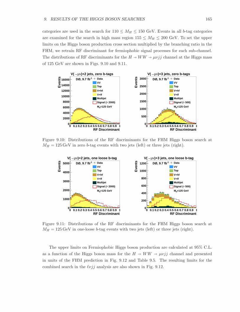
2.4 Search for the SM Higgs Boson in Leptons plus Jets Final
States
Searching for the SM Higgs boson begins by looking for detector signatures that are con-
sistent with its production and final decay products. This thesis is focused on searches
in the final states containing leptons and jets, which have been carried out in two differ-
ent physics analyses at the DØ experiment, namely ZH � ℓℓbb and ℓνjj analyses. The
searches are performed using a data set of proton-antiproton collisions corresponding to
9.7 fb−1 of integrated luminosity collected with the DØ detector at a center of mass energy
of√s = 1.96 TeV.
2.4.1 The SM Higgs Boson Signal in ZH � ℓℓbb and ℓνjj Analyses
The SM Higss signal in ZH � ℓℓbb analysis
The ZH → ℓℓbb analysis searches for the Higgs boson produced in association with a Z
boson, with the Z decaying leptonically to a pair of µ+µ− or e+e− and the Higgs boson
decaying to a pair of bottom and anti-bottom quarks. The leading order Feyman diagram
for the ZH → ℓ+ℓ−bb signal process is shown in Fig. 2.10. Being more sensitive to the
production of a low mass Higgs boson, the ZH → ℓℓbb analysis performs the search for the
mass range 90 ≤MH ≤ 150 GeV.
The SM Higgs signal in the ℓνjj channel.
The ℓνjj analysis performs the search for the SM Higgs boson using events containing
one charge lepton (ℓ = e or µ), a significant imbalance in transverse energy (6ET) arising
from a neutrino, and two or more jets. It comprises searches for multiple signal processes,
WH → ℓνbb, H → WW → ℓνjj , and V H → VWW → ℓνjjjj (where V = W or
Z). Leading order Feyman diagrams describing three main signal processes are shown in
Fig. 2.11. In theWH → ℓνbb process, the Higgs boson is produced via associated production
with a W boson, then the Higgs boson decays into a b-quark pair and the W boson decays
2. THE STANDARD MODEL AND HIGGS PHYSICS 39
Figure 2.10: Feynman diagram of ZH → ℓℓbb signal.
into a charge lepton and a neutrino. The Higgs boson in the H →WW ∗ → ℓνjj process is
produced by either gluon-gluon fusion or VBF process and decays into a pair of W bosons,
then oneW boson decays to a charged lepton and an associated neutrino, the otherW boson
decays to a quark-antiquark pair that hadronizes into two jets of particles. In the V H →VWW → ℓνjjjj process, the Higgs boson is produced via associated production with a
weak boson V and decays into a pair ofW bosons, and then oneW boson decays leptonically
into a charged lepton and a neutrino, the other two weak bosons decays hadroncally into
four jets. A small contribution to the Higgs boson sinal coming from ZH production and
from the decay H → ZZ when one of the charged leptons from the Z → ℓℓ decay is not
identified in the detector is also consider in this analysis.
The three main Higgs boson production and decay channels considered in the ℓνjj
analysis are sensitive to different hypotheses for MH , the WH → ℓνbb process is more
sensitive to the low mass region, while the H →WW → ℓνjj and V H → VWW → ℓνjjjj
processes are more sensitive to the high mass region, but contribute some senstivity at
lower masses through decays piercing a virtual W boson. Therefore, the lνjj analysis is
performed the search in the mass range 90 ≤MH ≤ 200 GeV.
2.4.2 Background in ZH → ℓℓbb and ℓνjj Analyses
Searching for the SM Higgs boson is challenging, because its primary decays are similar to
prodigious backgrounds at hadron colliders. There are two types of background processes
that are considered in ZH → ℓℓbb and ℓνjj analyses:
• The physics background processes, W + jets, Z + jets, top-quark pair, single-top and
diboson productions, are simulated by Monte Carlo (MC).
• The instrumental background from multijet events is estimated through control sam-
ples in the data.
2. THE STANDARD MODEL AND HIGGS PHYSICS 40
(a) W H → ℓνbb
(b) H → W W → ℓνjj
(c) W H → W W W → ℓνjjjj
Figure 2.11: Feyman diagrams of the main SM Higgs signals in ℓνjj analyses.
2. THE STANDARD MODEL AND HIGGS PHYSICS 41
The Z + jets, top-quark pair, diboson production and multijets are background processes
contribute in both the ZH → ℓℓbb and ℓνjj analyses. For the ℓνjj channel, the production
of a W boson in association with jets and single top production are considered as two
dominated backgrounds.
W + jets and Z + jets
The largest contribution to the background in the ℓνjj channel comes from W +jets events
where the W boson is produced in association with quarks or gluons with the W boson
decaying leptonically and the quarks or gluons hadronizing into jets. The W + jets sample
can be split into W + LF and W + HF where the jets are initiated from light flavor quark
(u, d, s) and heavy flavor quarks (c, b), respectively.
(a) W + jets (b) Z + jets
Figure 2.12: Feynman diagrams for W + jets and Z + jets background
The most dominant background in the ZH → ℓℓbb channel arises from the Z + jets
process. Similar to W + jets, the Z + jets events are categorized in Z + LF and Z + HF.
The Z + jets events, where one charged lepton from Z boson decay is lost to detection,
can also mimic expected signal signatures in the ℓνjj channel. In fact, the second largest
background in the ℓνjj channel comes from those Z+jets events. Feyman diagrams shown
in Fig. 2.12 are examples for W + jets and Z + jets processes.
Top Pair Production
A leading order Feyman diagram of top pair production (tt) is shown in Fig 2.13. The
tt events can be background candidates for the ZH → ℓℓbb channel when both W bosons
decay leptonically. The tt events can also contribute background to the ℓνjj channel in the
case that one W boson decays leptonically.
Single Top Production
The top quark in single top events is produced via electroweak interaction either from a
s-channel or t-channel process as shown in Fig. 2.14 The top quark decays almost 100% of
the time to a bottom quark and a W boson. To make a contribution to the background
2. THE STANDARD MODEL AND HIGGS PHYSICS 42
Figure 2.13: Feynman diagram for top pair production
of the ℓνjj channel, the W boson in the final states of top quark production must decay
leptonically.
(a) s-channel (b) t-channel
Figure 2.14: Feynman diagrams for single top production
Diboson Production
A pair of weak bosons, WW , WZ or ZZ, are produced via diagrams as shown in Fig. 2.15.
The diboson events can be background candidates for both ZH → ℓℓbb and ℓνjj channels
when at least one of the boson decays leptonically.
Multijet
The only background in ZH → ℓℓbb and ℓνjj channels that is not simulated by MC is the
multijet background. The multijet events are produced via the strong interaction and do
not contain any isolated charged lepton (Fig. 2.16), but they still can pass the selection
criteria and mimic expected signal signatures in the cases that:
• A jet is misidentified as an electron.
• A photon is misidentified as an electron.
2. THE STANDARD MODEL AND HIGGS PHYSICS 43
(a) W W (b) W Z
(c) ZZ
Figure 2.15: Feynman diagrams for diboson production
• A lepton from decay products of a jet is identified as an isolated lepton.
The description of multijet processes is not precisely modeled by MC, therefore, a data-
driven method is used to determine this background. Details about techniques used to
derive this background are presented in Sec. 5.5.
Figure 2.16: One of tree level Feynman diagrams for a multijet process
2.4.3 Analysis Procedure in ZH → ℓℓbb and ℓνjj Channels
Event selection
Searching for the Higgs boson in both ZH → ℓℓbb and ℓνjj analysis begin with selecting
events based on corresponding signal topologies as well as the kinematic differences between
2. THE STANDARD MODEL AND HIGGS PHYSICS 44
signal and background. The selection criteria are designed to maximize both the signal
acceptance and background suppression in each channel.
Background estimation
After applying selection criteria, detailed studies of simulated background samples and es-
timated multijet background are necessary to ensure that data are well described by the
SM processes that dominate the selected events. Both shape and normalization of the mul-
tijet background are estimated from data. Corrections to background for the discrepancies
between data and simulation are derived separately for each channel. These are described
in detail in Sec. 5.6.
Tagging for b-quark jets
The b-tagging technique is applied in both channels to identifying jets originating from
b-quarks. It is used to enhance the signal and suppress background in ZH → ℓℓbb channel.
Considering the differences in signal compositions of different signal processes, the b-tagging
requirements are used in ℓνjj channel to divide data into sub-channels (WH → ℓνbb,
H →WW → ℓν and WH →WWW → ℓνjjjj) to improve the signal sensitivities.
Multivariate analysis
Based on the differences in kinematics between signal processes and various background
processes with the same final state, a number of physics quantities that have the potential
of discriminating signal from background are identified. Studies to evaluate the discrim-
inating power as well as the agreement between data and total simulated background in
the distribution of those kinematic variables are carried out in both ZH → ℓℓbb and ℓνjj
channels. The ZH → ℓℓbb analysis exploits a special technique, namely a “kinematic fit”,
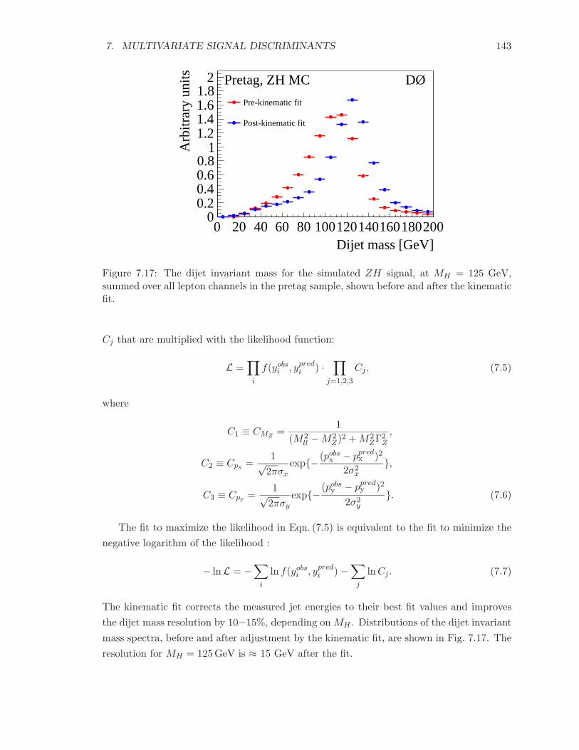
to improve the discriminating power of important variables. Finally, a list of good variables
is selected for each channels.
Multivariate Analysis (MVA) techniques are employed to incorporate discriminating
information from all selected variables into a single powerful discriminant to separate sig-
nal from background events. A boosted decision tree (bdt) implemented with the tmva
package [47] and a random forest decision tree (RF) [48] implemented in the statpattern-
recognition (spr) [49] package are two MVA techniques used in ℓνjj analysis. The RF
method and Matrix Element method, in which the final signal discriminant is built from
calculated probabilities of each observed event being from a signal or background process,
are applied in the ZH → ℓℓbb analysis.
2. THE STANDARD MODEL AND HIGGS PHYSICS 45
Assessing systematic uncertainties
The impact of systematic uncertainties on the shape and normalization of the MVA output,
the final discriminant distributions, for signal and each background process are assessed.
Correlations of each source of systematic uncertainty across all subsamples in each channel
are also considered.
Extracting the Higgs boson search results
The MVA output distributions in each channel along with associated systematic uncertain-
ties are used as inputs for the procedure of setting the upper limits on the SM Higgs boson
production cross section multiplied by the corresponding branching fraction in units of the
SM prediction. The 95% C.L. upper limits are determined on the Higgs boson production
cross section in the ranges of 90 ≤MH ≤ 150 GeV and 90 ≤MH ≤ 200 GeV for ZH → ℓℓbb
and ℓνjj channels, respectively, in steps of 5 GeV. The search in the ℓνjj channel is also
interpreted in the context of fermiophobic and fourth generation models.
The analysis procedure in both ZH → ℓℓbb and ℓνjj channeles will be described in
this thesis. Research procedures where the author of this thesis mainly contributed will
receive more detailed discussion. For the ℓνjj channel, the thesis focuses on the process of
background estimation, optimizing the MVA for the sub-channel H → WW → µνjj and
the SM Higg boson search results, as well as interpretation in the fermiophobic and fourth
generation models in this sub-channel. For the ZH → ℓℓbb channel, the thesis focuses on
the kinematic fit process and Matrix Element approach in discriminating Higgs boson signal
from backgrounds. The main Higgs boson search results in ZH → ℓℓbb and ℓνjj channel are
published separately in Refs. [50] and [10]. The Higgs boson searches in these two channels
are also combined with searches in other channels at the DØ and CDF experiments and the
combined results published in [12] and [13].
3. THE EXPERIMENT 46
3
The Experiment
3.1 The Tevatron
The Fermilab Tevatron is the world’s highest energy proton-antiproton (pp) collider with
center-of-mass collision energy√s = 1.96 TeV. Providing beams of such high energy requires
a complex accelerator chain to produce and accelerate particles. A diagram depicting the
Fermilab accelerator chain is shown in Fig. 3.1 [51].
Figure 3.1: Fermilab accelerator chain
At the first step, hydrogen gas is ionized into electrons and protons by electric pulses in
an ionization chamber. The released protons strike a negative electrode coated with cesium
in the chamber and produce hydrogen ions, (H−). The H− ions are focused toward the
Cockcroft-Walton pre-accelerator and accelerated to 750 keV. They are then steered to the
3. THE EXPERIMENT 47
linear accelerator (Linac) where they are accelerated to 400 MeV and grouped together to
form bunches spaced 5 ns apart by the oscillating electric fields of radio frequency (RF)
cavities.
Leaving the Linac, the 400 MeV H− ion beam is injected into the Booster, a synchrotron
accelerator, through a carbon foil where the two electrons are stripped off from each H−
ion, leaving a beam of bare protons. The magnetic field in the Booster bends the trajectory
of the protons making them move along the ring and the energy of protons is boosted from
400 MeV to 8 GeV by RF cavities. The 8 GeV beam of protons then goes to a transfer line
that leads to the Main Injector.
A part of the proton beam injected in the Main Injector is accelerated to 120 GeV
for creating antiprotons and the remainder is accelerated to 150 GeV for feeding into the
Tevatron. Antiprotons are produced by colliding the 120 GeV proton beam on a fixed
nickel target at the rate of about one antiproton created for each 105 incident protons
on the target with a wide energy spectrum and a large angular spread. The outgoing
antiproton beam is focused by magnetic lenses and undergoes a “cooling” process which
shrinks the kinetic energy spectrum of the beam to a mean value of 8 GeV. The antiprotons
are then accumulated and formed into 36 bunches of about 3 × 10¹⁰ antiprotons before
being transfered back into the Main Injector. This 8 GeV antiproton beam is subsequently
accelerated to 150 GeV together with 36 bunches of about 3 × 10¹¹ protons and injected
into the Tevatron.
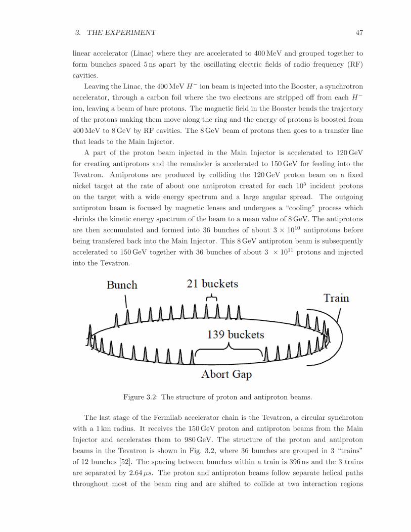
Figure 3.2: The structure of proton and antiproton beams.
The last stage of the Fermilab accelerator chain is the Tevatron, a circular synchroton
with a 1 km radius. It receives the 150 GeV proton and antiproton beams from the Main
Injector and accelerates them to 980 GeV. The structure of the proton and antiproton
beams in the Tevatron is shown in Fig. 3.2, where 36 bunches are grouped in 3 “trains”
of 12 bunches [52]. The spacing between bunches within a train is 396 ns and the 3 trains
are separated by 2.64µs. The proton and antiproton beams follow separate helical paths
throughout most of the beam ring and are shifted to collide at two interaction regions
3. THE EXPERIMENT 48
located around the centers of the DØ and CDF detectors. To enhance the interaction rate,
quadrupole magnets are used to focus the beams at each collision region.
3.2 The DØ Detector
Two detectors, CDF and DØ, were built around two collision regions of the Tevatron
to record and study the outcome of pp collisions. The design and performance of the
DØ detector, used to collect the data presented in this thesis, are described in detail in
Refs. [53, 54, 55, 56]. The major components of this multipurpose detector are shown in
Fig. 3.3 and listed from the innermost to the outermost location from the beam pipe as
follows:
• Central tracking system
• Preshower detector
• Calorimeter
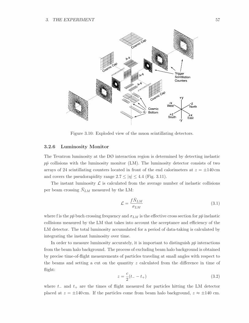
• Muon system
Figure 3.3: Cross sectional side view of the DØ detector.
The major components of the detector as well as the triggering and data acquisition systems
will be briefly described in the next sections.
3. THE EXPERIMENT 49
3.2.1 Coordinate System
In the detector description and data analysis we use a right-handed coordinate system which
has z-axis along the direction of proton beam and the y-axis pointing upward as in Fig. 3.3.
The (x, y) plane is transverse to the derection of the colliding beams. The angles θ and φ are
the polar and azimuthal angles, respectively, and the r coordinate denotes the perpendicular
distance from the z-axis.
The pseudorapidity, defined as η = −ln(tan θ2), is commonly used in experimental par-
ticle physics as a spatial coordinate. The pseudorapidity of a particle approximates its
Lorentz-invariant rapidity, which is defined in terms of energy (E) and longitudinal mo-
mentum (pz) of the particle as y = 12 ln(tanE+pz
E−pz), in the limit that its invariant mass is
much less than its energy m/E → 0. If the η quantity is calculated with respect to the
center of the detector, it is called detector eta and denoted as ηdet. If the η quantity of a
particle is calculated based on its reconstructed trajectory from the beam axis, it is called
physics eta and denoted as η.
3.2.2 Central Tracking System
Figure 3.4: Schematic view of the central tracking system.
The central tracking system of DØ detector consists of the Silicon Microstrip Tracker
(SMT) and the Central Fiber Tracker (CFT) embedded in a 2 T magnetic field provided
by a superconducting soneloid. The magnetic field bends the path of the charged particles
created from the pp collisions and the charged particles interact with the SMT and CFT
leaving patterns of hit points. The two tracking detectors record the tracks of the charged
3. THE EXPERIMENT 50
particles with |ηdet| < 3 and locate the pp primary interaction vertex with a resolution of
about 35µm along the beamline. A schematic view of the central tracking system is shown
in Fig. 3.4.
Silicon Microstrip Tracker
Located closest to the beam pipe, the SMT is designed for tracking charged particles near
the interaction points with a high resolution. It is constructed from six silicon barrels,
twelve F-disks and four H-disks as shown in Fig. 3.5.
Figure 3.5: Isometric view of the silicon microstrip tracker.
The central region of the SMT comprises six barrels which are arranged along the beam
axis with the centers at |z| = 6.2, 19.0, 31.8 cm. Each barrel s capped at high |z| with an
F-disk and has four silicon readout layers, which are set at the distance 2.7, 4.5, 6.6 and
9.4 cm with respect to the beam pipe. An unit of three F-disks is assembled on each side
of the central region. In the far forward region of the SMT, four H-disks are installed at |z|= 100.4 and 121.0 cm to provide tracking information at high |ηdet|.
In 2006, an inner layer called Layer 0 was inserted between the innermost layer of the
barrels and the beam pipe to improve tracking resolution and to compensate for radiation
damage at the first silicon layer of the barrels [57].
Central Fiber Tracker
The CFT consists of scintillating fibers arranged in eight concentric cylinders and occupies
the radial space from 20 to 50 cm from the beam axis. Waveguide fibers are coupled to scin-
tillating fibers to transfer the scintillating light produced by an incident charged particle
to visible light photon counters (VLPCs) for read out. The CFT provides additional infor-
mation to determine the momentum of charged particles and reconstruct tracks in region
|ηdet| ≤ 2.5.
3. THE EXPERIMENT 51
Solenoid Magnet
To improve the detector performance, a superconducting solenoidal magnet was installed
in the available space between CFT and the calorimeter: 2.73m in length and 1.42 m in
diameter. In order to optimize the momentum resolution and tracking pattern recognition
the solenoidal magnet was designed to create a central magnetic field of 2 Tesla. The magnet
operates stably at either polarity and the polarity of the magnetic field in the tracking system
is frequently reversed to reduce any detector asymmetry effects.
3.2.3 Preshower Detectors
Preshower detectors are made of thin layers of scintillator strips interspersed with lead ra-
diators. They are placed in front of the calorimeter and function as tracking detectors as
well as calorimeters. They help with electron identification and background rejection during
both triggering and offline reconstruction by enhancing the spatial matching between tracks
and calorimeter showers. Since particles like electrons and photons may interact with ma-
terials in the solenoid and create electromagnetic showers before entering the calorimeters,
having the preshower detector in front of calorimeters improves energy reconstruction in
the downstream calorimeters.
Figure 3.6: Location of major components of the DØ detector.
The DØ preshower detectors including the central preshower detector (CPS) located
between the solenoid and the central calorimeter and two forward preshower detectors (FPS)
3. THE EXPERIMENT 52
mounted on the end calorimeter are shown in Fig. 3.6. The CPS detector covers the central
region |ηdet| ≤ 1.3 and the two FPS detectors cover the forward region 1.5 ≤ |ηdet| ≤ 2.5.
3.2.4 Calorimeter System
The DØ calorimeter system was designed to assist in identification of electrons, photons, and
jets, as well as provide energy measurements of those objects, and measure the transverse
energy imbalance in events. The system consists of three sampling calorimeters located in
separate cryostats, the central calorimeter (CC) and two end calorimeters (EC), and an
intercryostat detector (ICD) (see Fig. 3.6). An illustration of the three main calorimeters is
shown in Fig. 3.7(a). The central calorimeter covers the region |ηdet| < 1 and the two end
calorimeters extend the coverage to |ηdet| < 4. In the transition region 1.1 ≤ |ηdet| ≤ 1.4
between CC and EC cryostats, calorimeter coverage is supplemented by the intercryostat
detector (see Fig. 3.7(b)).
(a) Isometric view of the calorimeter (b) Schematic view of the calorimeter
.
Figure 3.7: Overview of the DØ calorimeter.
Central Calorimeter and End Calorimeters
Particles created from pp collisions traverse material in calorimeters and lose their en-
ergy through different interaction processes resulting from the electromagnetic and strong
forces [58]. The types of energy-loss mechanisms that play a role depend on the nature and
the energy of the particle. Bremsstralung from electrons and the e+e− pair production from
photons are the dominant physics processes governing high-energy electromagnetic showers
initiated by electrons, positrons or photons. Meanwhile, the hadronic showers initiated by
high energy hadrons subject to strong interactions develop based on nuclear interactions.
Differences in the primary interactions giving rise to electromagnetic and hadronic showers
have crucial consequences in the development of the showers. The longitudinal length and
lateral spread of electromagnetic showers are governed by the radiation length (X0), which
mainly depends on the electron density of the material, while the dimensions of hadronic
showers depend on the nuclear interaction length (λint), which depends mainly on nuclear
3. THE EXPERIMENT 53
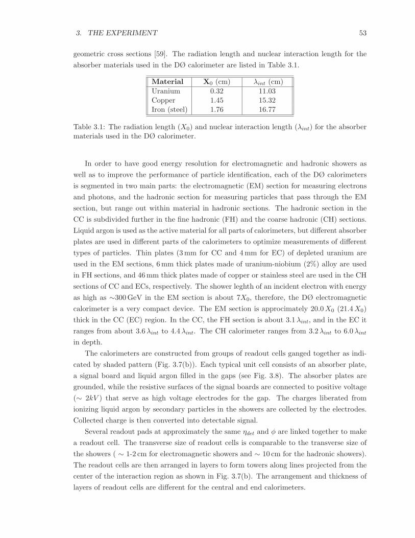
geometric cross sections [59]. The radiation length and nuclear interaction length for the
absorber materials used in the DØ calorimeter are listed in Table 3.1.
The electron identification efficiency (ID efficiency) of data at each working point is de-
termined using the “tag-and-probe” method based on Z → e+e− candidates having the
di-electron mass within the window of 80 < Mee < 100 GeV [62]. The electron ID efficiency
is defined as :
ǫ =Ntag
Nprobe(4.4)
where Nprobe is the number of electron candidates passing the selection cuts relevant to
the working point, and Ntag is number of electron candidates passing another set of more
stringent selection cuts to reduce the non-Z background and ensure a sample of high purity
electron candidates.
4. EVENT RECONSTRUCTION 66
The electron ID efficiency in MC simulation is calculated similarly based on the Z →e+e− MC sample and using the same selection cuts as for data. The number of MC events
passing the corresponding set of selection cuts and within the mass window is used to
determine the MC efficiency. The ID efficiency of both data and MC are parameterized as
a function of η and φ components of the electron.
To take into account the imperfection in detector simulation, an efficiency correction is
applied to MC samples by scaling the weight of MC events by a factor of ǫdata
ǫMC.
Energy calibration correction and resolution
An absolute calibration of the response of the EM calorimeter is derived based on Z → e+e−
events considering the boson Z mass as a calibration point. The measured electron energies
consequently are corrected by scaling up so that the mass peak in Z → e+e− matches the
value determined at the LEP collider. The correction is about 0.5 % and 0.1% in the CC
and ECs regions, respectively.
In general, the energy resolution of a calorimeter σE depends on fluctuation in the physical
development of the shower, the electronic noise of the readout system and other instrumental
effects. For a sampling calorimeter as in DØ detector, the fractional energy resolution can
be expressed as [63]:
(σE
E)2 =
S2
E+N2
E2+ C2 (4.5)
Where the parameters S, E, and C represents different contributing sources to the energy
resolution:
• S represents the stochastic term, which is related to fluctuations, and depends on the
choice of the absorber, active material and the thickness of sampling layers.
• N is related to electronic noise and depends on the features of the readout circuits.
The noise contribution to the energy resolution is dominant at low energy.
• C represents the constant term, which includes contributions from instrumental effects,
such as non-uniformity of material thickness, non-uniformity in charge collection,
mechanical imperfections, and does not depend on the energy of the particles.
The stochastic term of the electron energy resolution in the DØ calorimeter is determined
by test-beam data, while the noise term is determined by electronics studies and considered
to be 0.29 GeV for both CC and EC regions [64]. The constant term is dominant in the
high energy regime, and is evaluated by using Z → e+e− events. It is approximately 4%
(2%) for CC (ECs) region [64].
4. EVENT RECONSTRUCTION 67
4.2.2 Muon Identification
Muons deposit a very small amount of energy (only about few GeV) in the calorimeter
and can traverse the entire DØ detector. Therefore, in principle, muons are reconstructed
based on the tracking information they leave in the muon detector and the central tracking
system.
Muon reconstruction and identification criteria
The muon reconstruction algorithm employed by the DØ Collaboration can be divided into
the following main steps:
• Hit finding
The muon hits (impact positions of muons in the muon system) are determined by
using the scintillator counters and the drift time of the wire chambers.
• Segment reconstruction
The 2D track segments in the plane orthogonal to the toroidal magnetic field are
built by fitting trajectories to hits in the muon wire chambers. And then identified
segments are compared with scintillator hits for timing information on the segment.
• Local muon track finding
Track segments in the A-layer before the toroid and BC-layer after the toroid are
matched to form local muon track if they are consistent with the passage of a particle
through the magnet. For each compatible pair of segments, a local muon track is
reconstructed through a fit taking into account the toroidal magnetic field strength
and multiple scattering in the toroids.
• Matching with central tracking
The local muon tracks are matched to the tracks reconstructed in the central tracking
system to improve the accuracy of the muon kinematic properties. In the matching
process, the tracks are propagated through the calorimeter, taking into account the
inhomogeneous magnetic field, energy loss and multiple scattering.
The identification quality of a muon candidate is defined based on the quality of local
and central muon tracks as well as the isolation of muon from particles originating from
quark fragmentation and other heavy hadron decay products. To reconstruct the candidate
W (→ µν) or Z(→ µ+µ−) boson in our analyses, the muon candidates in selected events
are required to fulfill the following criteria:
• Local muon track with medium quality
To be identified as a local muon with medium quality, the muon candidate must have
at least one scintillator hit and two wire hits in the A layer as well as in BC layers. A
veto against cosmic muons was imposed by demanding that the scintillator hit times
4. EVENT RECONSTRUCTION 68
in the A and BC layers be consistent with the travel time for a particle moving at the
speed of light from the primary vertex (|tA|, |tBC | < 10 ns).
• Central muon track with medium quality
The selected muon candidates are required to have matched tracks in the central
tracking system with medium quality. A central track is defined as “medium” if (i)
the track distance of closest approach to the beam axis |dca| is less than 0.04 cm and
the track contains SMT hits or |dca| < 0.02 cm for the track without SMT hits, (ii)
it has at least two hits in the CFT, and (iii) χ2/NDOF < 4 where χ2 is the result of
the fit used for reconstruction of the track in the central tracking system and NDOF
is the number of degrees of freedom in the fit.
• Loose or tight isolated muon
Muons coming from leptonic decay of W or Z bosons tend to be isolated from jets,
while muons originating from decays of heavy hadrons are typically non-isolated due to
fragmentation products of hadronic decay. Five discriminating variables were formed
to select isolated muons:
– The distance in the (η, φ) space of the muon to the nearest jet with pT > 15 GeV,
∆R(µ, jet) =√
∆η(µ, jet)2 + ∆φ(µ, jet)2.
– The scalar sum of transverse momenta of tracks within the ∆R < 0.5 cone around
the muon, Itrk = Σ(∆R<0.5)ptrkT .
– The sum of transverse energies of all calorimeter clusters in the hollow cone
0.1 < ∆R < 0.4 around the muon, Ical = Σ(0.1<∆R<0.4)EclusterT .
– Two additional isolation variables, Itrk/pµT and Ical/pµ
T , were employed to offer
stringent rejection of leptons from b-quark and c-quark decays.
The loose isolated muons are required to have ∆R(µ, jet) < 0.5. The tight isolated
muons are required to have ∆R(µ, jet) < 0.5, Itrk/pµT < 0.12 and and Ical/pµ
T < 0.40.
In the loose muon samples used to estimate multijet background in our analyses, we require
that the muons satisfy the above tracking requirements and the loose isolation criteria. The
tight muon events selected to extract the Higgs boson signal in our analyses are required to
contain muons satisfying the same tracking requirements as for the loose muon sample and
the tight isolation criteria.
Muon identification efficiency and momentum resolution
The performance of the DØ detector in identifying and reconstructing muons is quantita-
tively assessed in terms of muon identification efficiency and momentum resolution [65]. In
the region |η| < 2, the efficiency of muon system reconstruction of muon candidates used in
4. EVENT RECONSTRUCTION 69
our analyses ranges from 75% to 90%. Central tracks matched to these muons are recon-
structed with average efficiency of 90.5%. The isolation criteria reject multijet background
with efficiencies ranging from 87% to 92% depending on quality requirements. The momen-
tum of a muon candidate is taken to be the momentum measured in the central tracking
system and the momentum resolution of typically 10% for pT = 40 GeV.
4.2.3 Jet Identification
Jet development
Jets result from the fragmentation of quarks and gluons generated in the hard scattering
process of pp collisions. The development of jets in the detector can be separated into three
sequential stages:
• Quarks and leptons are produced from the hard scattering process, and then these
partons can eventually radiate additional partons and form “parton jets”.
• Stable particles produced through hadronization of quarks and gluons, excluding un-
detected muons and neutrinos, are clustered to form “particle jets”.
• The spray of produced hadrons interact inside the calorimeter where the “calorimeter
jet” is defined and its energy is measured.
A sketch of the evolution from a hard-scatter parton to a jet in the calorimeter is shown in
Fig. 4.1.
Jet reconstruction
Jets are reconstructed using the Run II cone algorithm [66], which is an iterative cone
algorithm used to build jets from energy deposits in the calorimeter. The first step of
jet reconstruction is defining the jet seeds by clustering pseudoprojective towers in η ×φ calorimeter cells. Each cell is treated as a massless object and has an associated 4-
momentum computed using the direction defined by the primary vertex and the center of
the cell and assuming E = |p|. The 4-momentum of a pseudoprojective tower is formed by
combining the 4-momentum of calorimeter cells using the E-scheme:
P tower = (Etower,−→P ) =
∑
i=cells in tower
(Ei,−→pi ). (4.6)
The calorimeter towers are ordered in decreasing transverse momentum and used to
form preclusters within a cone of radius 0.3 in the (η, φ) plane, starting with the tower
having the highest pT and descending the list until no towers above the minimum threshold
pT > 500 MeV remain. Preclusters with pT > 1 GeV are used as seeds for the jet clustering
algorithm.
4. EVENT RECONSTRUCTION 70
Figure 4.1: The evolution from a hard-scatter parton to a jet in the calorimeter.
The seeds are then used as center points and all calorimeter towers around the seeds
within the cone of radius Rcone = 0.5 (∆R =√
(∆y)2 + (∆φ)2 < Rcone) are combined
to form the proto-jets. The 4-momemtum of a proto-jet is the sum of the 4-momenta
of all included calorimeter towers. When the direction of the 4-momentum of the proto-
jet does not coincise with the cone axis, the process is repeated using the direction of
the proto-jet 4-momentum as the new center point for the cone until a stable solution is
found. To reduce the sensitivity to soft radiation, mid-points between pars of two proto-
jets are also used additional seeds, if the distance between two proto-jets is in the range of
Rcone ≤ ∆R ≤ 2Rcone. Any proto-jets having the transverse momentum below a minimum
threshold pT (protojet) < 3 GeV are discarded.
The obtained proto-jets may contain partially overlapping or identical jet candidates.
To avoid double counting tower energies the proto-jets are sorted in order of decreasing
pT and processed through a split-or-merge procedure to remove overlaps. Two proto-jets
are merged into one jet if they have an overlap region containing more than 50% of the
transverse momentum of the lower pT proto-jet. Otherwise, two proto-jets are split into
two jets and each cell in the overlap region is assigned to the nearest jet in the (y, φ)
plane. The jet 4-momentum is recomputed after the split-or-merge process and the jets
with pT < 8 GeV are discarded.
4. EVENT RECONSTRUCTION 71
Jet identification
To eliminate jet candidates not originating from outgoing partons of the hard scattering
process, a set of jet identification criteria are imposed:
• Requirement on the electromagnetic fraction: 0.05 < EMfrac < 0.95.
The energy fraction in the EM layers is required to be less than 95% in order to reject
electron- and photon-like objects. The requirement of having electromagnetic fraction
higher than 5% has to be fulfilled to reject fake jets coming from noises in the hadronic
calorimeter.
• Requirement on the coarse hadronic fraction: CHfrac < 0.40.
The energy fraction in the outermost layer of the calorimeter, the coarse hadronic
layer, is required to be less than 40%. This requirement is designed to further remove
jets that are formed predominantly out of the noise in the hadronic calorimeter.
• L1 trigger confirmation
A Level 1 trigger confirmation is obtained by requiring the jet energy measured by the
independent electrical readout of L1 to be larger than 50% of the jet energy, excluding
the energy deposited in the coarse hadronic calorimeter cells (CH is not included at
L1). This removes jets formed out of noise, such as coherent noise in the precision
readout electronics.
• Vertex confirmation
To ensure a selection of jets originating from the hard scattering process, the criteria
of a jet to be vertex confirmed are imposed. A vertex confirmed jet must be associated
with at least two tracks orginating from the primary vertex. These tracks must have
pT > 0.5 GeV, at least one hit in the SMT, distance of closest approach to the beam
line in the transverse plane DCAxy < 0.5 cm, distance of closest approach to the beam
line in the z direction DCAz < 1 cm, and ∆z(vertex, track) < 2.0 cm.
Jet energy scale
The jet energy scale (JES) corrects on average the energy of jets measured in the calorimeter
to the corresponding particle jets. This correction accounts for the differences in the observ-
able jets from the particle level due to detector and jet algorithm effects [67]. Correcting
the jet energy measured in the DØ detector Emeas to the particle level Eparticle is performed
in three stages: (i) correction of offset energy (O), (ii) correction of jet energy due to the
calorimeter response (R), (iii) correction for showering effects (S). These corrections can
be expressed by the formula:
Eparticle =Emeas −O
R · S . (4.7)
The main effects considered when calibrating jet energy will be briefly discussed before
evaluating the final JES. Additional corrections for small biases in the method are described
4. EVENT RECONSTRUCTION 72
elsewhere [67].
• Offset energy correction (O)
The offset energy consists of the energy in the jet that is not related to the primary
pp interaction. It includes a component corresponding to energy from multiple pp
interactions during a bunch crossing (MI) and a component originating from electronic
noise, calorimeter noise from uranium decay and the pile-up energy from other bunch
crossing (NP). The value of the MI offset depends linearly on the number of additional
interactions, which is characterized by the number of reconstructed pp interaction
vertices (NPV ) in a given event. Fig. 4.2 shows the offset correction as a function
of jet pseudorapidity in the detector for different numbers of reconstructed primary
vertices. The uncertainties on the offset corrections are of the order of 1% of the
overall energy correction at low jet pT and are negligible for jet pT above ∼ 100 GeV.
-2.0 -1.5 -1.0 -0.5 0.0 0.5 1.0 1.5 2.00.0
0.5
1.0
1.5
2.0
2.5
3.0
= 0.7coneR
= 4PV
N
= 3PV
N
= 2PV
N
= 1PV
N
Eoff
set /
cosh(�
det)
(G
eV
)
�det
-1DØ, 0.70 fb
Figure 4.2: Offset corrections for different primary vertex multiplicities.
• Calorimeter response correction (R)
The calorimeter response R is the average fraction of the energy measured in the
calorimeter for the particles inside the jet cone. It is factorized into two parts
R = RCC(E) × Fη(η,E), where the RCC term is an absolute response correction
determined from the CC region and the relative response correction term Fη normal-
izes the response of the calorimeter as a function of jet pseudorapidity.
Absolute response correction
The response for jet energies in the CC region is derived by using the pT balance
between the γ and the jet in the γ + jet events. To have a clean γ + jet data sample,
only photons with tight selection criteria in the CC region are used. The jet is required
to be back-to-back to the photon (∆φ(γ,jet) > 2.9) and no additional jets are allowed
in selected events. At the particle level, the transverse momenta of the photon and
4. EVENT RECONSTRUCTION 73
the hadronic recoil system are balanced each other:
−→P T,γ +
−→P T,jet =
−→0 . (4.8)
Due to non linearities in the energy response of the calorimeter, the measured jet
PT,jet becomes unbalanced with the photon PT,γ causing a non-zero 6ET:
Rjet·−→P T,jet +Rγ · −→P T,γ = −−→6ET , (4.9)
where Rjet and Rγ are electromagnetic and hadronic energy responses of calorimeter,
respectively. Using the corrected photon energy scale (Rγ =1.0) and projecting Eq. 4.9
onto the direction of photon transverse momentum , the jet response is defined as:
Rjet = 1 +
−→6ET · −→P T,γ
|−→P T,γ |2. (4.10)
The jet energy response in the CC region shown in Fig. 4.3 is measured as a function
of:
E′ = pT,γ · cosh(ηjet), (4.11)
which is highly correlated with the particle level jet energy and has finer resolution
than the measured jet energy. The dependence of jet response to E′ is later mapped
to the measured jet energy to determine the correction to be applied to the specific jet
algorithm. The dominant sources of uncertainty on jet pT response come from photon
identification, photon energy scale, fragmentation and PDF, and the total uncertainty
is about ∼ 1%.
Figure 4.3: Fits of the jet energy response in the CC region using MC points (solid line)and data (dotted line) [67].
4. EVENT RECONSTRUCTION 74
Relative response correction
The relative response correction, Fη, calibrates forward jets with respect to central
jets. It normalizes the response at forward pseudorapidities to that measured in the
CC region (RCC) and is defined as:
Fη(E, η) ≡R(E, η)
RCC(E), (4.12)
where R(E, η) is the response of detector for a jet of energy E, located at detector
pseudorapidity η. Deriving Fη is based on the pT balance in two samples, γ + jet
and dijet. For the dijet sample, one of the jets is required to be in the CC and the
response measurement is binned in E’ using the pT of the central jet after correcting
for offset and central calorimeter response. The η-dependence of the relative response
is parameterized as a quadratic-logarithmic function of E’:
Fη(E′, η) =
p0(η) + p1(η)ln(E′) + p2(η)ln2(E′)
RCC(E′), (4.13)
where pi are fitted as functions of η. Fig. 4.4 shows the η dependence correction in
the region of 0.8 < η < 0.9 for the γ + jet and dijet samples. The difference in Fη fits
observed in Fig. 4.4 is due to the different amount of quark and gluon jets in the γ+jet
and dijet samples. The gluon initiated jets have lower response than quark initiated
jets since they have on average higher particle multiplicity with softer particles.
E' (GeV)
-1DØ, 0.70 fb
Figure 4.4: Fits of Fη in γ + jet and dijet as a function of E’ [67].
• Showering correction (S)
Showering effects contribute to the mismeasurement of jet energy due to the net flow
of energy in and out of the jet cone caused by detector effects, such as the magnetic
4. EVENT RECONSTRUCTION 75
field, scattering from passive material, and shower development in the calorimeter.
The determination of the showering correction is based on comparison of jet en-
ergy profiles between MC and data using a sample of back-to-back γ + jet events.
Energy density profiles of jets in MC are generated as a function of the distance
∆R =√
(yparticle − yjet)2 + (φparticle − φjet)2 between the particle and jet axis. The
calculated energy profile in MC is fitted to measured energy profile after the offset
correction has been applied. An example of energy profiles as function of ∆R for MC
and data in one η, pT bin is given in Fig. 4.5. It shows the good agreement between
measured energy in data and the sum of energy contributions originating from inside
and outside the particle jet. The showering correction in each (η, pT ) bin is estimated
102-1
DØ, 0.70 fb
101
100
10-1
10-20.0 0.5 1.0 1.5 2.0 2.5 3.0 3.5
ΔR
0.0 ≤ |ηdet
jet| < 0.4, 45 ≤ p
T' < 60 GeV
<E
(ΔR
)> (
Ge
V)
Figure 4.5: Showering profiles as function of distance from jet axis ∆R for data and MC [67].
as:
S =ΣRcone
∆R=0Ein + ΣRcone
∆R=0Eout
ΣR∞
∆R=0Ein
, (4.14)
where ΣRcone
∆R=0Ein is the energy of the particle jet deposited inside the jet cone, ΣRcone
∆R=0Eout
is the energy deposited inside the jet cone from particles outside the jet, and ΣR∞
∆R=0Ein
is the total enegy of particle jet obtained using the fit-weighted templates.
The systematic uncertainties on the showering correction are mainly driven by the
quality of the template fit, the physics modeling of jet fragmentation and the purity
of the γ + jet sample. They are less than 1% of the overall correction factor at
pT < 50 GeV.
4. EVENT RECONSTRUCTION 76
Shifting, smearing and removing in simulated jets
In order to correct simulated jets for the differences with data in terms of energy scale,
resolution and reconstruction efficiency, the JSSR procedure which allows simulated jets to
be smeared, shifted and possibly removed was developed [68]. In the JSSR procedure, the
corrections of simulated jets were derived using the γ + jet and Z + jet samples where γ/Z
and jet in each selected events are required to be back-to-back in azimuth to avoid large
effects from QCD radiation. Determination of these corrections relies on the measurement
of the transverse momentum imbalance in selected γ + jet and Z + jet events:
∆S =pjet
T − pγ/ZT
pγ/ZT
, (4.15)
which was binned in pγ/ZT separately in different η region. An example of the ∆S distribution
for data and MC are given in Fig. 4.6. The ∆S distribution in each pT , η bin is fitted
Figure 4.6: ∆S distributions for data (left) and Monte Carlo (right). The full curves showthe fits using a fitted function composed of a Gaussian and an error function. The yellowbands denote statistical error. The dashed curves correspond to the extrapolation of thegaussians to the region effected by the jet reconstructed threshold.
with a function composed of a Gaussian and an error function to count for resolution and
efficiency effects [68, 69]. The full curves in Fig. 4.6 show the fit results and the dashed
curves correspond to the extrapolation of the gaussians to the region effected by the jet
reconstructed threshold. These fits provide simultaneously information on:
• the jet energy resolution via the width of the Gaussian.
• the jet energy scale via the central value of the Gausian
• the jet reconstruction and identification efficiency via the error function.
Smearing
4. EVENT RECONSTRUCTION 77
The jet transverse energy resolution in data and MC can be deduced from the corre-
sponding Gaussian width of the ∆S distribution:
σGauss∆S =
σpT
pγ/ZT
. (4.16)
The smearing process corrects for jet resolution differences in data and MC by scaling
the transverse momentum of simulated jets with a smearing factor which is randomly drawn
from a new Gaussian having width computed as:
σsmearing =√
σ2∆S(Data) − σ2
∆S(MC), (4.17)
where σ2∆S(Data) and σ2
∆S(MC) are the gaussian width of the ∆S distribution measured in
data and Monte Carlo, respectively. Fig. 4.7 shows the width of smearing factor Gaussian
for simulated jets in CC region as a function of pZT .
>, GeVZT
<p0 20 40 60 80 100 120 140 160 180
2 MC
σ-2 D
ATA
σ
-0.04
-0.03
-0.02
-0.01
0
0.01
0.02
0.03
0.04
MC smearing for CC Jets
Figure 4.7: Square of the width of the smearing factor Gaussian as function of pZT for CC
jets. The parametrization and the statistical error are represented by the blue curve andthe yellow band.
Shifting
The imbalance between transverse energies of the Z/γ and jet is provided by the mean
< ∆S >Gauss of the Gaussian in the ∆S distribution. Fig. 4.8 shows the difference in the
imbalances obtained in data and simulation < ∆S >Data − < ∆S >MC , which presents
the data-MC relative jet energy scale (JES).
The fact that the data and MC transverse energies do not coincide results from different
effective jet reconstruction thresholds and from different amounts of out-of-cone radiation
in data and MC. To correct for this difference, the relative JES is parameterize as a function
of pγ/ZT and a shifting factor extracted from the fit is applied to the jet transverse energy in
4. EVENT RECONSTRUCTION 78
>, GeVZT
<p0 20 40 60 80 100 120 140 160 180
>M
CS∆
> -<
DAT
AS∆<
-0.2
-0.15
-0.1
-0.05
0
0.05
0.1
0.15
MC shifting for CC Jets
Figure 4.8: The shifting factor as function of pZT for CC jets. The parametrization and the
associated error from the fit are represented by the blue curve and the yellow band.
MC.
Similar to the JES correction, the shifting correction also depends on the flavor of the
partons initiating jets. Figure 4.9 shows the difference in Gaussian means between data
and MC as a function of jet pT in Z+1jet events for quark jets (primarily u, d or s quarks)
and gluons. The data-MC relative JES is consistent with 0 for quark jets, while tending to
be shifted downwards for gluon jets. The b-jets are know to be broader than light quark
jets and that makes them more gluon-like. Therefore, the shifting correction is effectively
applied to those physics processes with gluon or b-quark dominated final states.
Figure 4.9: Relative JES of data and MC for quark (blue) and gluon (magenta) jets. Thered line shows the nominal JSSR jet shifting for an ensemble of jets with both quark andgluon components. Hashed lines represent statistical errors.
4. EVENT RECONSTRUCTION 79
Undergoing the smearing and shifting procedures, the corrected jet pT is obtained by
first smearing simulated jets according to the parameterization shown in Fig. 4.7, and then
their energies are shifted according to the parameterization shown in Fig. 4.8:
where shift(pT ) is the shifting factor and Gauss(0, smear(pT )) is a gaussian function cen-
tered at 0 and with a width shown in Fig. 4.7 as a function of pT .
Removal
The fitted efficiency turn-on curves displayed in Fig. 4.10 present the dependence of jet
reconstruction and identification efficiency on the jet pT in various calorimeter regions [69].
In both data and simulation, the full efficiency is reached at ∼ 15 GeV, which is taken as
the threshold for jet removal. The jets with pT < 15 GeV are randomly removed from the
MC to match the efficiency in data [68].
Figure 4.10: Average efficiency turn-on functions represented for different calorimeter re-gions fo data (left) and simulation (right).
4.2.4 Missing Transverse Energy
The presence of neutrinos in the final state of an event at the detector level is inferred from
the missing transverse energy, which is the energy imbalance of an event in the transverse
plane perpendicular to the beam. The raw 6ET, which results from physics objects that
escape the detector without energy deposits like neutrinos or from instrumental sources such
as a calorimeter noise and physics object resolution, is measured by vectorially summing
the calorimeter cells transverse energy:
−→6ETraw
= −cells∑−→6ET . (4.19)
4. EVENT RECONSTRUCTION 80
The cells from the coarse hadronic layers of the calorimeter are not included in the sum
since they suffer from relatively high noise (usually have higher noise and negative energy
cells). The energy and momentum corrections applied to EM objects, muon and jets are
propagated to the measured 6ET and the corrected 6ET is obtained by:
−→6ET = −cells∑−→6ET
corrected −muons∑ −→pT , (4.20)
where∑−→pT is the sum of muon transverse momentum measured by the muon spectrometer.
4.2.5 b-jet Identification
Since the H → bb decay mode is the most important search at the Tevatron for the SM
Higgs boson with MH < 135 GeV, identifying jets initiated from b-quarks (referred to as
b-jet identification or b-tagging) is the main key for Higgs physics at the DØ. The facts that
the mass of the b-quark is substantially larger than that of light flavor quarks (u, d, s, c) and
the life time of the b-quark is sufficiently long for b-hadrons to be formed and travel a few
millimeters before the b-quark decays lead to special signatures for b-jets observed in the
detector. Various algorithms have been developed in the DØ collaboration to exploit the
properties of b-jets in order to detect their presence. The performance of identifying b-jets
is improved significantly by using a neural network (NN) tagger to combine information
obtained from different b-tagging algorithms into a final discriminant to distinguish b-jets
from other jet flavors. Details about the b-tagging methods developed by the DØ experiment
are described in Ref. [70].
b-jet properties
The long lifetime and fragmentation properties of b-quarks allow us to use precise track-
ing information to identify b-jets though their decay products. The secondary vertex con-
structed from the tracks produced by the b-hadron decay products and the impact parameter
(distance of closest approach of tracks to the primary vertex) are important features con-
sidered in b-tagging algorithms. Furthermore, b-hadron decays often lead to the production
of high momentum leptons, which can provide easy access to samples with enhanced b-jet
content. An illustration for reconstructing the secondary vertex and measuring the impact
parameter of a b-jets is shown in Fig. 4.11.
b-tagging prerequisites
The requirements for a jet to be taggable, i.e., for it to be further investigated by the b-
tagging algorithms, is that it must contain at least two tracks where each track has at least
one hit in the SMT, the “seed” track must have pT > 1 GeV while the other track must
have pT > 0.5 GeV, and the distance of each track to the primary vertex must be < 2 mm
in the transverse plane and < 4 mm in the z direction.
4. EVENT RECONSTRUCTION 81
Figure 4.11: Reconstructed secondary vertex and impact parameter (d0) in a b-jet.
The efficiency for taggability is defined as the ratio of the number of taggable jets over
the number of calorimeter jets. It accounts for variations in detector acceptance and track
reconstruction efficiencies at different locations of the PV and is determined as a function of
jet kinematics (pT and η) and the z coordinate of the PV. To optimize the use of geometrical
correlations between η and z, the taggability is parametrized in z′ ≡ |z|sign(η · z) as shown
in Fig. 4.12.
z’ (cm)-60 -40 -20 0 20 40 60
Tag
gabi
lity
0
0.1
0.2
0.3
0.4
0.5
0.6
0.7
0.8
0.9
1
all jets
> 40 GeVT
jets with p
a)
Figure 4.12: Taggability as a function of z′.
4. EVENT RECONSTRUCTION 82
b-tagging algorithms
Several algorithms to identify b-jets exploiting the long lifetime and decayed products of
b-quarks and have been developed in the DØ Collaboration. They are based entirely on
tracking and vertexing of the charged particles.
• The secondary vertex tagger (SVT)
The SVT is the most intuitive b-tagging algorithm which exploits the fact that b-
hadron decays give rise to multiple charged particles emanating from the b-hadron
decay point. It is developed based on the reconstruction of this decay point and re-
quirement of the presence of a secondary vertex. The algorithm starts from selecting
tracks associated with a taggable jet and then requires that a number of tracks are
extrapolated to the same point in three dimensions. Secondary vertices are associ-
ated with the calorimeter jet if ∆R(vertex, jet) < 0.5, where the vertex direction is
computed as the difference of the secondary and primary vertex position.
• The jet lifetime probability tagger (JLIP)
The JLIP algorithm combines the impact parameters of all tracks associated with a
calorimeter jet into a single variable, the jet lifetime probability PJILP , which can be
interpreted as the confidence level that all tracks in a jet originate from the selected
primary interaction point. Jets from light quark fragmentation are expected to have
an uniform PJILP distribution between 0 and 1, while a peak at close to 0 is expected
in PJILP distribution of jets from b- or c-quarks. A jet is tagged as b-jet if the PJILP
is below an upper threshold which is set based on the signal efficiency and background
rejection designed for a given analysis.
• The counting signed impact parameter tagger (CSIP) The CSIP algorithm
selects “good” tracks with a certain quality within a R = 0.5 cone around the jet axis
and computes the signed impact parameter significance Sd for each selected tracks [70]:
Sd =IPs
σ(IPs), (4.21)
where IPs is the signed impact parameter and σ(IPs) is the uncertainty on the mea-
surement of IPs. A jet is considered to be b-jet by the CSIP tagger if there are at
least two good tracks with Sda > 3 or at least three good tracks with Sd
a > 2, where
a is a scaling factor. The choice of a determines the b-tagging efficiency and mistag
rate of the algorithm.
The Neutral Network (NN) b-tagger
The b-tagging algorithms described above exploit different features of the b-hadron and
perform separately to distinguish b-jets from other jet flavors. To improve the tagging
4. EVENT RECONSTRUCTION 83
efficiency with respect to any single algorithm, the NN b-tagger combines discriminating
information provided by the SVT, JLIP and CSIP tagging algorithms into a single final
discriminant to separate b-jets from light jets (where “light” stands for uds-quark or gluon).
The NN was trained on simulated light flavor and bb samples using nine input variables.
Six of the variables are based on the secondary vertex reconstructed by the SVT algorithm,
and the remaining three variables are obtained using the JLIP and CSIP algorithms. The
description of these variables is given in Ref. [70]:
• SVT Sxy: the decay length significance (the decay length in the transverse plane
divided by its uncertainty) of the secondary vertex with respect to the primary vertex.
• SVT χ2dof : the χ2 per degree of freedom of the secondary vertex fit.
• SVT Ntrk: the number of tracks used to reconstruct the secondary vertex.
• SVT mvtx: the mass of the secondary vertex.
• SVT Nvtx: the number of secondary vertices reconstructed in the jet.
• SVT ∆R: the distance in (η, φ) space between the jet axis and the difference between
the secondary and primary vertex positions.
• JLIP PJLIP : the jet lifetime probability computed by JLIP algorithm.
• JLIP PRedJLIP : PJLIP re-calculated with the track with the highest significance
removed from the calculation.
• CSIP NCSIP : a combined variable based on the number of tracks with an impact
parameter significance greater than an optimized value.
The output from the optimized NN b-tagger on bb and light-flavor simulated jets given in
Fig. 4.13 shows a significant separation between the signal and background samples.
NN Output-0.2 0 0.2 0.4 0.6 0.8 1 1.2
Nor
mal
ized
Fre
quen
cy
0
0.05
0.1
0.15
0.2
0.25
0.3
0.35
0.4 b-jets
light-jets
Figure 4.13: The NN output for light-flavor jets (dashed line) and b-jets (continuous line)with pT > 15 GeV and |η| < 2.5 in simulated QCD events. Both distributions are normalizedto unity.
4. EVENT RECONSTRUCTION 84
The larger cut values on the NN output set a tighter b-tagging working point. Table 4.3
lists several operating points with associated b-tagging efficiency and light-flavor mistag rate
(fake rate) for jets in CC region.
Operating point Loose Medium Tight
NN output 0.45 0.65 0.77b-jet efficiency 60.8% 53.7% 47.6%
Fake rate 2.02% 0.96% 0.55%
Table 4.3: The b-tagging operating points with associated efficiency and fake rate.
5. SIGNAL PREDICTION AND BACKGROUND ESTIMATION 85
5
Signal Prediction and Background
Estimation
5.1 Data Samples
The search for SM Higgs boson production and decay processes that can lead to the final
states containing leptons and jets presented in this thesis uses the full data set corresponding
to 9.7 fb−1 of integrated luminosity of pp collisions at a center-of-mass energy of√s =
1.96 TeV collected with the DØ detector.
The most crucial step in our analyses is selecting a sub-dataset of events which have
topologies similar to the signatures of the targeted SM Higgs boson signals. However, various
SM processes can mimic the expected signal signatures, and thus need to be considered as
potential background. In order to find the SM Higgs boson or exclude its existence, it is
essential to have deep understanding of the differences in the properties of the SM Higgs
signal and background processes at the detector level. Therefore, MC simulated signal and
background samples are produced based on SM prediction to model compositions of data.
The differences in kinematics of simulated signal and background events are then exploited
to build a mathematical tool for differentciating signal events from background events in
data.
There are two major data subsamples collected with the DØ detector over two different
time periods. The first is the RunIIa data set taken from August 2002 until the 2006
shutdown, and the second is the RunIIb data set taken from June 2006 to September 2011.
Since important detector and trigger updates have been made between RunIIa and RunIIb,
two different sets of simulated MC samples have been used RunIIa and RunIIb to properly
describe the data.
5. SIGNAL PREDICTION AND BACKGROUND ESTIMATION 86
5.2 Monte Carlo Generators
Physics events recorded in the data samples are created from pp collisions through the
following processes:
• Initially two beams of protons and antiprotons are coming towards each other. Each
proton and antiproton involved in a pp collision is characterized by a set of parton
distribution functions (PDF) which defines the partonic substructure of the proton
and antiproton in terms of composition and momentum distribution.
• As p and p come into contact, partons from the p or p may start a sequence of
branchings with initial-state radiation (ISR) and build up initial-state showers.
• Two partons from initial-state showers originating from a pp pair undergo a hard
scatter process, and then a number of outgoing partons are produced. The nature of
this process determines the main characteristics of the event.
• The outgoing partons can start branching with final-state radiation (FSR) and build
up final-state showers. The gluons created in the shower can produce further quark
pairs, and that increases particle multiplicity in the final state of the event.
• The outgoing quarks and gluons are not directly observable, because they fragment
into neutral hadrons. Most of the hadrons produced during the fragmentation are
unstable and decay to final state particles forming jets, which finally are identified by
the detector. The process wherein the coloured partons are transformed into jets of
colourless hadrons, photons and leptons is called hadronization.
The evolution of a physics event as described above can be modeled by different Monte
Carlo generators, and the resulting observable signals can be studied using detailed detector
smulations. A brief description of these event generators is given in this chapter.
5.2.1 PYTHIA
The pythia Monte Carlo is a general-purpose event generator [71]. It allows generation
of complete events within the bounds of current understanding of the underlying physics.
The pythia generator as configured for these studies uses the CTEQ6L1 [72] leading order
parton distribution functions to model the initial partonic states for the hard parton scatter-
ing processes. The parton-shower approach, where the probability for a parton to branch
is given by evolution equations, is employed to model the ISR and FSR processes. The
hadronization process takes place at low Q2 where QCD perturbation theory breaks down.
It is codified in pythia based on the phenomenological model called “String Fragmentation”
with the assumption of linear confinement [71].
5. SIGNAL PREDICTION AND BACKGROUND ESTIMATION 87
5.2.2 ALPGEN
The alpgen generator is designed for the generation of complex and high-multiplicity hard
scattering final states in hadronic collisions. In this program, the tree level scattering
amplitude for multi-parton final states is computed based on a recursive numerical Leg-
endre transform of the effective action starting from the SM Lagrangian [73]. Using the
CTEQ6L1 parton distribution functions, alpgen provides the most accurate modeling for
the underlying hard processes of major backgrounds in our analyses, which have final states
containing a combination of electroweak bosons along with multiple quarks and gluons.
However, alpgen itself does not handle the showering and hadronization processes. To
complement the calculation of parton-level matrix elements with the evaluation of the full
hadronic structure of the final state, the parton-level calculations given by alpgen are
merged with the partonic evolution through interfacing with shower MC programs such as
pythia, herwig or isajet.
5.2.3 SingleTop
The SingleTop generator is a matrix element generator designed for simulating electroweak
single top-quark production in the next leading order (NLO) approximation [74]. The spin-
correlation effects in the single top-quark production are also considered in this program.
Subsequent parton shower and hadronization are provided via an interface with pythia.
5.2.4 MCFM
MCFM is a parton-level Monte Carlo program [75]. It is designed to calculate cross-sections
for various femtobarn-level processes at hadron colliders. For most processes, matrix ele-
ments are included to the next-to-leading order calculation and spin correlations are fully
incorporated.
5.2.5 MLM Scheme
The mlm matching scheme is a procedure for combining tree-level matrix element generators
with parton showers. The matching criteria developed in the mlm algorithm eliminate the
double counting of configurations where jets can arise from both the higher-order parton
level calculation and from hard emission during the shower evolution [76]. To properly
simulate events with high jet multiplicity in our analyses, the mlm algorithm has been
used to merge matrix elements of hard underlying processes generated by alpgen and the
subsequent development of the hard partons into jets of hadrons modeled by pythia.
5. SIGNAL PREDICTION AND BACKGROUND ESTIMATION 88
5.3 Detector Simulation
In the real world, the collider machine produces interactions and the events are observed
at the detector. Information about an event, particles produced and their momentum,
is reconstructed based on electronic signals from detector systems, such as sillicon and
scintillating fiber tracking systems, calorimeters and wire chambers.
In the Monte Carlo world, the generators play the role of collider machine producing
events. The behaviour of the DØ detector is fully simulated in two programs, the DØ
detector simulation DØgstar based on the detector material simulation package GEANT
and the simulation of DØ detector electronics and pileup interactions by DØsim. The
outputs of MC generators are used as inputs for DØgstar program and then passed to
DØsim. The DØgstar program models how particles produced by the event generator
interact with magnetic fields and material in the detector. The DØsim program models
detector noise, residual activity from previous beam crossings and contributions from the
presence of additional pp interactions. The output of the detector simulation has exactly
the same format as the real data recorded by the detector, and these events are fed into the
same program for event reconstruction as collider data.
5.4 Simulated Event Samples
A brief description of the main Higgs boson signal and background processes in the ZH →ℓℓbb and ℓνjj analyses was given in Sec. 2.4 of Chapter 2. Besides the main signal processes
introduced, we also include signal components not specifically targeted but which fall in our
acceptance criteria nonetheless. The following section presents details of the simulation of
the signal and background contributions in each analysis.
5.4.1 Simulated signal processes
Signal samples in ℓνjj analysis
In the ℓνjj analysis, we account for all SM Higgs boson production with and decay processes
that can lead to a final state containing exactly one charge lepton, a significant imbalance
in transverse energy (6ET), and two or more jets. The considered signal processes are
categorized by the production mode as the following:
• Associated production of a Higgs boson with a vector boson
(i) WH � ℓνbb: This is the most important signal process in the low Higgs mass
region, where the Higgs boson is produced in association with a W boson, the SM
Higgs boson decays to a bb pair and the W boson decays leptonically.
(ii) V H � V V V ∗� ℓνjjjj: In this process, the Higgs boson is also produced in
association with a vector boson (W or Z) and then decays into a pair of vector
5. SIGNAL PREDICTION AND BACKGROUND ESTIMATION 89
bosons. One vector boson decays leptonically, and two other vector bosons decay
hadronically producing four jets. The V H � V V V ∗� ℓνjjjj process contributes to
both low mass and high mass regions.
(iii) Additional topologies that are also considered in this context are WH � ℓνcc,
WH � ℓντ+τ−, ZH � l+l−bb. However, these three signal processes just play a
minor role in ℓνjj analysis, due to the low decay rates of H � τ+τ−, cc, and that,
the contributions from ZH � l+l−bb only arises when one lepton in the final state is
mis-identified and significant 6ET results from this mis-identification and/or poor jet
energy resolution.
• Gluon fusion production
(i) gg � H � WW ∗� ℓνjj: The Higgs boson is produced through the main produc-
tion channel, gg � H, and then decays into a pair of W bosons, where one W boson
decays leptonically and the other decays hadronically. This is the dominant signal
production process in the high Higgs mass region and it contributes to low Higgs
mass region as well.
(ii) gg � H � ZZ∗� l+l−jj: The Higgs boson in this process decays into a pair of
Z bosons, where one Z boson decays hadronically and the other decays leptonically
(with only one lepton identified). The contribution of this channel is rather small.
• Vector boson fusion production
(i)V BF � H � V V ∗� ℓνjj: The Higgs boson is produced through the vector boson
fusion mechanism and then decays into a pair of W or Z bosons, where one vector
boson decays leptonically (with exactly one identified lepton). The contribution of
this signal process is minor due to the small cross section of the SM Higgs production
through vector boson fusion.
Signal samples in ZH � ℓℓbb analysis
• The ZH � ℓℓbb analysis requires the final state to have two isolated charged leptons
(either electrons or muons), at least two jets and at least one jet must satisfy a tight
b-tagging requirement. Besides the main signal process ZH � l+l−bb (where the
Higgs boson is produced in association with a Z boson, then the Higgs boson decays
into a pair of b-quarks and the Z boson decays into a pair of charged letons), we also
consider ZH � l+l−cc and ZH � l+l−τ+τ− signal processes. The ZH � l+l−bb
signal component accounts for more than 90% of the total signal yields.
All SM Higgs signal processes considered in our analyses are simulated with the Monte Carlo
event generator pythia at leading order. The signal samples involving H � bb, H � cc or
H � τ+τ− decays are produced in the mass range 90 - 200 GeV in 5 GeV steps. The signal
samples involving H � V V ∗ decays, which dominate the sensitivity of high mass searches,
Figure 5.2: Muon efficiency ǫℓLT parametrization as a function of muon pT . The red andblue lines are the fit uncertainties.
branching ratio of the process, Lint is the integrated luminosity used in the analysis, and
Ntot is the total number of generated events in each MC samples.
Besides physics motivated corrections, which are applied to MC samples to account for
higher-order calculations of cross sections as described above, we also consider another class
of corrections used to compensate for possible higher order corrections to specific physics
final states and detector modeling variations in the simulations. Processes of deriving
corrections for these modeling effects are commonly called reweighting. The corrections
coming from reweighting processes are derived in form of scale factors which can be constant
or have a kinematic dependency. MC samples are then corrected through scaling the weight
of simulated events accordingly.
Most corrections related to detector effects are integrated into the DØ analysis frame-
work, and they are applied in our analyses. To further improve the data modeling and
mitigate discrepancies in kinematic distributions, we derive an additional set of corrections
based on specific samples and selection criteria to further correct the V + jets (W + jets
and Z+jets) sample, the largest background in our analyses. Brief descriptions of common
corrections implemented in the DØ framework and details of our own V + jets reweighting
process are given in the following sections.
5.6.1 Reconstruction Efficiency Corrections
Lepton Reconstruction Efficiency Corrections
Scale factors are applied to MC events to account for differences in reconstruction efficien-
cies between the data and simulation for leptons and jets. For the MC electrons, a scale
factor correcting for electron identification (ID) efficiency is parameterized and applied as
a function of detector η, detector φ and instantaneous luminosity [62]. Similarly, multiple
scale factors have been parameterized as functions of detector η and φ and applied to MC
5. SIGNAL PREDICTION AND BACKGROUND ESTIMATION 97
muons to correct for muon identification efficiency, muon track reconstruction efficiency and
muon isolation efficiency [89].
The electron energy scale correction parameterized in detector azimuthal angle φ, physics
η of the electron and kinematic variables describing shower shape is applied to both data
and MC samples. Subsequently, the difference in electron energy resolution of data and
MC, which is caused by imperfect descriptions of the material in front of the calorimeter
and approximations in the shower development used in the DØ simulation programs, is
corrected by electron energy smearing process [90]. The resolution of muon momentum is
also not described perfectly in MC. Therefore, the muon transverse momenta reconstructed
in MC are smeared to bring MC into a better agreement with data [91].
Jet Reconstruction Efficiency Corrections
To correct on average the jet energy of jets measured in the calorimeter to the corresponding
particle jets and for the differences in jet energy resolution predicted in MC and observed
in data, JES and JSSR processes described in Chapter 4 are applied to MC samples ac-
cordingly. The efficiency of vertex confirmation for jets and the efficiency for a jet to be
taggable are also corrected in simulated samples to reproduce the respective efficiencies in
data. Both vertex confirmation and taggability scale factors are parameterized as a function
of jet pT , jet η, and the Z-coordinate of the primary vertex [92].
Since performance of the b-tagging algorithm is different in data and simulated samples,
the tagging rate function (TRF) in MC is not the same as that in data [70]. To correct
for this effect, the b-jet identification scale factor (SFib) for jets to pass a specific b-tagging
working point (i) is applied to each corresponding b-tagged data sample.
5.6.2 Trigger Correction
The effect of trigger selection is simulated in the MC sample by applying the trigger effi-
ciency, measured in data, as an event weight to each MC event. The trigger efficiency used
in our analyses is parametrized as a function of electron or muon η, azimuthal angle, and
transverse momentum pT . More details about trigger selection and trigger efficiency will
be presented in Chapter 6.
5.6.3 Luminosity Reweighting
In order to provide a realistic simulation of the detector response to beam conditions during
actual data collection, an overlay of zero bias data collected using zero-bias triggers is used
to define the baseline detector response for each MC event. However, the instantaneous
luminosity for the zero-bias overlay does not match the luminosity profile of the dataset
under analysis. Therefore, a luminosity reweighting is apply to match the instantaneous
luminosity profile in MC to the luminosity profile of the data.
5. SIGNAL PREDICTION AND BACKGROUND ESTIMATION 98
5.6.4 Primary Vertex Reweighting
Due to the emittance growth of the colliding beams, the width of the distribution of the
primary vertex longitudinal position Vz becomes broader later in the store. The width of
Vz measured in data depends on the intensity profile of the proton and antiproton beams,
the amplitude and oscillation of the transverse motion of bunches, while the Vz distribution
used in simulating MC events is based on a Gaussian of a fixed width. Therefore, a primary
vertex reweighting is used to correct the generic primary vertex distribution in MC to the
distribution measured in data.
5.6.5 ZpTand WpT
Reweighting
Due to the softscale of radiation emission back-to-back with the vector boson, the Z boson
pT and W boson pT distributions are poorly modeled by both pythia and alpgen for
events with pZT or pW
T less than 30 GeV. The transverse momentum spectrum of the Z boson
is corrected in the MC to match that observed in data by reweighting the ZpTdistribution.
The correction is derived from the pZT distribution at the generator level and the observed
spectrum in the unfolded data [93]. The pZT reweighting scale factor is applied to simulated
events as a function of pZT in each bin of jet multiplicity. The W boson pT distribution is
also corrected using the same dependence, taking into account differences between the pT
spectra of Z andW bosons predicted in NNLO QCD [94, 95].
5.6.6 V + jets Reweighting
After all standard corrections for physics modeling and detector effects implemented in the
DØ framework have been applied to preselected samples in our analyses, the kinematic
distributions in data and simulated events show remaining residual differences in several
kinematic distributions. Motivated by comparisons of MC events simulaed with alpgen
and data [96], and MC samples simulated with other event generators [76], we develop
corrections to W + jets and Z + jets MC samples to correct for the shape discrepancies
in kinematic distributions between data and simulation. The corrections are derived based
on the direct comparison between selected data and MC events passing our preselection
criteria (before applying b-tagging), where any contamination from signal is very small.
To improve the description of the jet directions, we correct the η distributions of the
leading and second leading jets ( jets with the highest and second highest transverse mo-
mentum) in V + jets events. The lepton η distribution in W + jets (Z + jets) MC events in
the ℓνjj (ZH � ℓℓbb) analysis is also corrected to reproduce the distribution of final state
leptons associated with W/Z decays in data. Correlated discrepancies observed in distribu-
tions of transverse momentum pWT of the leptonically decaying W boson and the jet angular
separation between two leading jets, ∆R(j1, j2) =√
(ηjet1 − ηjet2)2 + (φjet1 − φj2)2, are
corrected simultaneously in the two-dimensional (∆R(j1, j2), pWT ) plane [97].
5. SIGNAL PREDICTION AND BACKGROUND ESTIMATION 99
Eta-2.5 -2 -1.5 -1 -0.5 0 0.5 1 1.5 2 2.5
500
1000
1500
2000
2500
3000
3500
j2eta_data j2eta_dataEntries 107290
Mean 0.008629
RMS 1.14
j2eta_data
-2.5 -2 -1.5 -1 -0.5 0 0.5 1 1.5 2 2.5
500
1000
1500
2000
2500
3000
j2eta_data j2eta_dataEntries 71122Mean 0.01031
RMS 1.154
j2eta_data
Eta-2.5 -2 -1.5 -1 -0.5 0 0.5 1 1.5 2 2.5
V+J
ets
Rat
io
0
0.2
0.4
0.6
0.8
1
1.2
1.4
1.6
j2eta_data fit_j2eta_dataEntries 43574
Mean 0.03293
RMS 1.549
j2eta_data j2eta_dataEntries 107290
Mean 0.008629
RMS 1.14
Eta-2.5 -2 -1.5 -1 -0.5 0 0.5 1 1.5 2 2.5
500
1000
1500
2000
2500
3000
3500
j2eta_data j2eta_dataEntries 107290
Mean 0.008629
RMS 1.14
j2eta_dataEntries 107290
Mean 0.008629
RMS 1.14
j2eta_data
Figure 5.3: Performance of the second leading jet η reweighting. The top-left plot showsdata (points) and all backgrounds (blue) before reweighting; the top-right plot shows thenon-V + jets background-subtracted data (points) and V + jets sample (red); the bottom-left plot shows the fit to the ratio of non-V + jets background-subtracted data and V + jetsbackground; the bottom-right plot shows data (points) and all backgrounds (blue) afterapplying the second jet reweighting.
Jet η Reweighting
Due to the deficiencies in the MC programs and the parameters that are used in the event
generation, the jet η distributions of the V + jets samples generated by alpgen interfaced
with pythia do not agree with our data. In particular, the η-distributions observed in
data are broader than in simulation. To compensate for the observed deviations we apply
reweighting scale factors to each generated event in the W + jets and Z + jets MC samples
to better match the observed data. Two reweighting processes are applied in succession,
the first one is for the η distribution of the second leading jet (ηjet2) followed by another
for the η ditribution of the leading jet (ηjet1).
The jet η reweighting procedure starts with normalizing the total number of W + jets
and Z+jets MC events to the number of events in the V +jets component of data (NdataV +jets),
5. SIGNAL PREDICTION AND BACKGROUND ESTIMATION 100
which is is obtained by subtracting the MJ background (NMJ) and other non-W + jets or
non-Z + jets SM background sources (NMCnonV jets) from the selected data sample Ndata :
NdataV +jets = Ndata −NMJ −NMC
nonV jets. (5.14)
The jet η reweighting scale factor is then parameterized as function of jet η based on the
ratio of jet η distributions between simulated V + jets sample and data after subtraction
of the none V + jets backgrounds and :
f(η) = p0 + p1 × η2 + p2 × η4 + p2 × η4. (5.15)
The normalization of the V +jets sample is constrained during the fit for the parameters
pi of the reweighting function (Eqn. (5.15)). The agreement in the distribution of ηjet2
between data and MC before and after applying ηjet2 reweighting along with the fit based
on preselected samples of ℓνjj analysis are show in Fig. 5.3 .
Lepton η Reweighting
To account for mismodeling of lepton directions in the ℓνjj analysis, we reweight theW+jets
samples using a second-order polynomial reweighting function of lepton η (ηlepton):
f(ηlepton) = p0 + p1 × η2lepton, (5.16)
which is extracted from the ratio of lepton η distributions between simulatedW+jets sample
and data after subtracting QCD and the other non-W + jets physics background. Similar
to the jet η fitting procedure, the W + jets sample is first normalized to the corresponding
background-subtracted data, and the normalization is constrained during the fitting. The
lepton η reweigting is also applied in the ZH � ℓℓbb analysis where the distribution of
leading pT lepton in the Z+jets sample is corrected to that of background-subtracted data.
∆R(j1, j2) and pW
TReweighting
To account for residual discrepancies in modeling the pWT and the separation of the two
leading jets ∆R(j1, j2) as well as for strong correlation between these two kinematic vari-
ables, we perform a simultaneous fit in both pWT and ∆R(j1, j2) using the two dimensional
reweighting function fpWT
× f∆R, where:
fpWT
= a0 + a1 × [1 − erf(pW
T − a2
a3)] + a4 × exp(
−0.5 × (pWT )4
a25
), (5.17)
f∆R = b0 + b1 × ∆R + b2 × (∆R)2 + c3 × (∆R)3.
The ai and bi parameters in the pair of fpWT
and f∆R reweighting functions are determined
from the 2D fit in the (∆R(j1, j2), pWT ) plane to the ratios of W + jets MC sample to the
5. SIGNAL PREDICTION AND BACKGROUND ESTIMATION 101
Figure 5.4: The 2D reweighting in the (pWT , ∆R(j1, j2)) plane: (left) Ratio of background-
subtracted data (points) and simulated W + jets, (right) 2D fitting function fpWT
× f∆R.
non-V + jets component of the data, which is obtained by subtracting the MJ background
and other non-W + jets SM background sources from the data sample (see Fig. 5.4). The
pWT reweighting is applied only to W + jets events, while the ∆R(j1, j2) reweighting is
applied to both W + jets and Z + jets events.
Reweighting functions from each V + jets reweighting process are shown in Fig. 5.5.
The corrections derived from each V + jets reweighting procedure is designed to change
differential distributions, but to preserve normalization. The distributions of ηjet2, ηjet1,
pWT , and ∆R(j1, j2) in data and MC before and after appying all corrections from V + jets
reweighting procedures are shown in Fig. 5.6. These corrections are on the order of a few
percent in the highly populated region of each distribution and may exceed 10% in the
extreme values of each distribution.
5. SIGNAL PREDICTION AND BACKGROUND ESTIMATION 102
η Leading Jet nd2-2.5 -2 -1.5 -1 -0.5 0 0.5 1 1.5 2 2.5
(bottom) and simultaneously correct for pWT and ∆R(j1, j2)) (middle). In each plot, the
black curve represents the nominal reweighting function, while the red and blue curvesrepresent ±1σ variations on the fit function.
5. SIGNAL PREDICTION AND BACKGROUND ESTIMATION 103
-2.5 -2 -1.5 -1 -0.5 0 0.5 1
Eve
nts
Jet_eta21.5 2 2.5
500
1000
1500
2000
2500
3000
eta2_dataeta2_data
-2.5 -2 -1.5 -1 -0.5 0 0.5 1
Eve
nts
Jet_eta11.5 2 2.5
500
1000
1500
2000
2500
3000
eta1_dataeta1_data
0 1 2 3
Eve
nts
DeltaR(j1, j2)4 5 6
0
2000
4000
6000
8000
10000
dr_datadr_data
0 20 40 60 80 100 120 140 160
Eve
nts
WpT180 200
0
1000
2000
3000
4000
5000
6000
7000
wpt_datawpt_data
Figure 5.6: Distributions of ηjet2, ηjet1, pWT , and ∆R(j1, j2) in data (black) and MC before
(red) and after (green) appying all corrections from V + jets reweighting.
6. EVENT SELECTIONS 104
6
Event Selections
Event selection in both ℓνjj and ZH → ℓℓbb analyses is based on signal signatures and
kinematics. The ℓνjj analysis requires topologies with an isolated charged lepton and a
significant imbalance in the transverse energy, which indicates products of W � eν or
W � µν decays, and at least two jets. The ZH → ℓℓbb analysis requires two isolated
charged leptons to reconstruct the Z candidate decaying as Z � e+e− or Z � µ+µ− and
at least two jets. The selection criteria in each analysis are designed to maximize the
acceptance of the considered SM Higgs boson signals and to suppress the background as
much as possible, while maintaining good data-to-MC agreement in the preselected sample.
Taking into account the differences in background composition and signal topologies,
the search in each analysis is then organized into sub-channels according to various lepton,
jet multiplicity, and b-tagging characterization criteria in order to optimize the overall signal
sensitivity. The event selection proceeds in two steps, online event selection (event trigger-
ing) and offline event selection. Both selection steps along with the channel subdivisions in
each of ℓνjj and ZH → ℓℓbb analyses are described in this chapter.
6.1 Event Selection in ℓνjj Analysis
6.1.1 Online Event Selection
Event triggering in electron channel (eνjj)
Events in the electron channel have the final state containing an electron candidate expected
from W � ℓν decays. These are triggered by a logical OR of Single-Lepton and Lepton+Jets
triggers requiring a candidate electromagnetic object and jets [98]. The trigger efficiency
is parameterized as a function of the transverse momentum pT and and η of the leading
electron candidate in the event, and it is applied as an event weight to simulated samples.
For the events selected in our analyses, these triggers have a typically efficiency of above
90%.
6. EVENT SELECTIONS 105
Event triggering in muon channel (µνjj)
For the muon channel, we accept events fired by any available trigger, except those contain-
ing lifetime-based requirements that can bias the performance of b-jet identification. The
efficiency of this inclusive set of triggers is obtained by applying a trigger correction, Pcorr,
to the efficiency of a well-modeled logical OR of the Single-Muon and Muon+Jets triggers
(TµOR). The correction is derived from comparing data events selected with TµOR triggers
to events selected using all triggers:
Pcorr =(NData −NMJ)incl − (NData −NMJ)TµOR
NMC, (6.1)
where the numerator is the difference between the number of data events in the inclusive
trigger sample and the TµOR trigger sample, after subtracting off the multijet (MJ) back-
grounds, and the denominator is the number of MC events with the trigger efficiency set to
1. The inclusive trigger efficiency estimate for events in the muon channel is TµOR + Pcorr
(limited to be ≤ 1).
Using the inclusive set of triggers results in a gain of about 30% in efficiency over
using only Single-Muon and the Muon+Jets triggers (TµOR ∼ 70%). The most significant
contribution to this improvement comes from triggers based on jets and 6ET. To account
for the differences in the contribution and the efficiency of different triggers, the inclusive
trigger correction Pcorr is parametrized as a function of the scalar sum of the transverse
momenta of all jets, HT , and the 6ET for separate regions in muon η.
(GeV)TH50 100 150 200 250 300
corr
P
0
0.2
0.4
0.6
0.8
1
1.2 -1DØ, 9.7 fb(a)
< -1.2φ-2 < > -1.2φ < -2, φ
<50 GeVTE
(GeV)TH50 100 150 200 250 300
corr
P
00.20.40.60.8
11.21.41.6 -1DØ, 9.7 fb
(b)
< -1.2φ-2 < > -1.2φ < -2, φ
50 GeV≥TE
Figure 6.1: Data-derived muon trigger correction to account for the resulting efficiency gainin moving from single muon and muon+jets triggers to inclusive triggers as a function of HT
for |η| < 1.0, shown (a) for events with 6ET < 50 GeV and (b) for events with 6ET < 50 GeV.The black circles show the correction when the muon is in the region of φ (−2 < φ < −1.2),where the detector support structure allows only partial coverage by the muon system, andthe red triangles show the correction elsewhere in φ.
6. EVENT SELECTIONS 106
6.1.2 Offline Event Selection
The preselection of events for the eνjj or µνjj channel includes events satisfying a set of
selection criteria based on the identification and kinematics of physics objects in the final
state. The selection cuts applied for each channel are discussed in the following sections.
• Primary vertex selection
The event selection in both electron and muon channels requires a pp interaction
vertex that has at least three associated tracks, and is located within 60 cm of the
center of the detector along the beam direction (PVz ≤ 60 cm). If an event has more
than one such vertex, the vertex with the highest average pT -value of its associated
tracks is chosen. This requirement ensures that selected events are from collisions
occurring in the central part of the detector, where the activity from the primary
interaction can be covered by the SMT and physics objects in event final state are
more likely to be within the detector acceptance.
• Lepton selection
The requirement of the final state to contain exactly one isolated electron or muon
candidate coming from the leptonic decay of a W boson significantly suppresses the
multijet background and that from Z(→ ℓℓ) + jets and tt events. Two sets of lepton
identification criteria are applied for each lepton channel in order to form a “tight”
sample used to perform the search for the SM Higgs boson and a “loose” sample used
to estimate the multijet background as described in Sec. 5.5.
For the electron channel, events having a single electron with transverse momentum
pT > 15 GeV within a pseudorapidity range of |η| < 1.1 (CC) or 1.5 < |η| < 2.5
(EC) are selected. We exclude the gap situated between the central and the end-cap
calorimeter in the pseudorapidity range of 1.1 < |η| < 1.5. The electrons passing the
kinematic selections above are further required to satisfy identification criteria, which
are optimized separately for the CC and EC regions. The two sets of identification
criteria used to select tight and loose electron samples for each calorimeter region are
listed in Table 4.2.1 (Sec. 4.2.1).
For the muon channel, we select events having exactly one muon with pT > 15 GeV and
|η| < 2.0. Muon candidates are then required to fulfill identification criteria related
to the muon track quality and the isolation of muon from particles originating from
hadron decay products, which are defined in Sec. 4.2.2. Selected events in the loose
or tight samples must contain a muon candidate with a medium quality local track
identified in the muon system matched to a medium quality central track. The muons
in the tight and loose samples are required to satisfy the tight and loose isolation
criteria, respectively.
• Missing transverse energy selection
6. EVENT SELECTIONS 107
To reconstruct the candidate W (→ ℓν) boson, selected events are required to con-
tain a significant 6ET, which characterizes the presence of the neutrino. The missing
transverse energy is reconstructed as described in Sec. 4.2.4, and is required to satisfy
6ET > 15 GeV for the electron channel and 6ET > 20 GeV for the muon channel. The
6ET cut is efficient in both removing mismodeled events and reducing the multijet
dominated region at low 6ET.
• Jet selection
Events considered in ℓνjj analyses are required to contain at least two jets originating
from the primary pp vertex. Besides satisfying the identification criteria described in
Sec. 4.2.3, these jets must have pT > 20 GeV and within |η| < 2.5.
To group events with similar signal-to-background ratio and optimize the search for
specific signal processes, the preselected sample of each lepton channel is then split
into three orthogonal subsamples based on jet multiplicity: two jet exclusive, three
jet exclusive and four jet inclusive. The dominant signal contribution in the two-
jet exclusive and three-jet exclusive channels comes from the WH � ℓνbb and H �
WW ∗� ℓνjj processes, while the majority of signal events in the four-jet inclusive
channel is from the V H � VWW ∗� ℓνjjjj process.
• Mutijet background veto
The transverse massMWT of the leptonically decayingW (→ ℓν) boson is reconstructed
from the (ℓ, 6ET ) system using missing transverse energy, the lepton transverse energy
(EℓT ), and the azimuthal separation ∆φ(ℓ, 6ET ) between the isolated lepton and the
6ET vector:
(MWT )
2 ≡ 2 pℓT 6ET [1 − cos ∆φ(ℓ, 6ET )].
Multijet events contribute a significant rate at small values of MWT and the signal-to-
background ratio is rather small at low 6ET region [99, 98]. Therefore, we apply a
triangular cut on the MWT :
MWT > 40 GeV − 0.5× 6ET ,
in order to suppress overwhelming background from multijet events (this is developed
using control samples in the data as described in Sec. 5.5).
6.1.3 Normalization at the Preselection
After applying the MC corrections described in Sec. 5.6 to simulated events, we adjust the
normalization of the V + jets and MJ backgrounds to bring the total number of predicted
background events in agreement with data. The normalization factors applied to V + jets
and MJ backgrounds are determined via a simultaneous template fit of the MWT distribution
to the V + jets and MJ component of data, which is obtained by subtracting non-V + jet
6. EVENT SELECTIONS 108
simulated background sources from the preselected data sample. We perform separate
fits for each lepton flavor and jet multiplicity category. Figure 6.2 shows examples of the
simultaneous fits for two and three jet exclusive samples in muon channel. The V + jets
experimental normalization factors for the two jet and three channels are 1.02 and 1.24,
respectively. The distribution of MWT after this normalization procedure along with the
distributions of muon pT and azimuthal angle between the muon and neutrino for the muon
channel are shown in Fig. 6.3. Distributions of the transverse momentum of the two jets
with the highest pT and the dijet mass reconstructed from them show good agreement
between data and combined background for preselected events in the muon channel (see
Fig. 6.4).
Figure 6.2: Simultaneous fit of the V +jets and MJ backgrounds in the W (→ ℓν) transversemass (MW
T ) distribution, in the muon two jet (left) and muon three jet (right) channels.The V +jets experimental normalization factors for the two jet and three channels are 1.02and 1.24, respectively.
6.1.4 Classifying b-tag Samples
To focus on the number and quality of identified b jets in preselected events, we define
six independent tagging samples based on the b-jet identification discriminant output (bID)
described in Sec. 4.2.5. The criteria for categorizing b-tag samples are as follows:
• a zero b-tag (0Tag) sample includes events with no jet satisfying the b-tagging criteria;
• a one-loose b-tag (1L) sample includes events with exactly one b-tagged jet that passes
the loose selection requirement (bID > 0.02) but fails the tight selection requirement
(bID > 0.15);
• a one-tight b-tag (1T) sample includes events having exactly one b-tagged jet that
has a b-identification discriminant output satisfying the tight b-jet selection threshold
(bID > 0.15);
• a two-loose b-tag (2L) sample includes events with two or more b-tagged jets that have
an average value of the b-identification discriminant of the two leading b-tagged jets
in the range 0.02 < (bj1ID + bj1ID)/2 ≤ 0.35;
6. EVENT SELECTIONS 109
[GeV]WTM
0 20 40 60 80 100 120
Eve
nts
0
5000
10000
15000
20000
25000
-1DØ, 9.7 fb)+2 jets, pretagνµ→V(
Data
VVTop
V+hf
V+lfMultijet
1000)×Signal (
=125 GeVHM
[GeV]WTM
0 20 40 60 80 100 120
Eve
nts
0
1000
2000
3000
4000
5000
6000
7000
8000 -1DØ, 9.7 fb
)+3 jets, pretagνµ→V(Data
VVTop
V+hf
V+lfMultijet
500)×Signal (
=125 GeVHM
[GeV]T
Muon p20 40 60 80 100 120
Eve
nts
0
2000
4000
6000
8000
10000
12000 -1DØ, 9.7 fb
)+2 jets, pretagνµ→V(Data
VVTop
V+hf
V+lfMultijet
1000)×Signal (
=125 GeVHM
[GeV]T
Muon p20 40 60 80 100 120
Eve
nts
0
500
1000
1500
2000
2500
3000
3500
4000 -1DØ, 9.7 fb)+3 jets, pretagνµ→V(
Data
VVTop
V+hf
V+lfMultijet
500)×Signal (
=125 GeVHM
)ν,µ(φ∆0 0.5 1 1.5 2 2.5 3
Eve
nts
0
5000
10000
15000
20000
25000
30000 -1DØ, 9.7 fb
)+2 jets, pretagνµ→V(
Data
VVTop
V+hf
V+lfMultijet
1000)×Signal (
=125 GeVHM
)ν,µ(φ∆0 0.5 1 1.5 2 2.5 3
Eve
nts
0
1000
2000
3000
4000
5000
6000
7000
8000
9000 -1DØ, 9.7 fb)+3 jets, pretagνµ→V(
Data
VVTop
V+hf
V+lfMultijet
500)×Signal (
=125 GeVHM
Figure 6.3: Kinematic distributions related to the lepton and 6ET for the two jet (left) andthree jet (right) event samples in the muon channel after preselection.
6. EVENT SELECTIONS 110
[GeV]T
Leading jet p20 40 60 80 100 120 140
Eve
nts
0
2000
4000
6000
8000
10000
12000
14000
16000
18000 -1DØ, 9.7 fb
)+2 jets, pretagνµ→V(Data
VVTop
V+hf
V+lfMultijet
1000)×Signal (
=125 GeVHM
[GeV]T
Leading jet p20 40 60 80 100 120 140
Eve
nts
0
500
1000
1500
2000
2500
3000
3500
4000 -1DØ, 9.7 fb
)+3 jets, pretagνµ→V(Data
VVTop
V+hf
V+lfMultijet
500)×Signal (
=125 GeVHM
[GeV]T
Leading jet pnd220 30 40 50 60 70 80
Eve
nts
0
5000
10000
15000
20000
25000
30000 -1DØ, 9.7 fb)+2 jets, pretagνµ→V(
Data
VVTop
V+hf
V+lfMultijet
1000)×Signal (
=125 GeVHM
[GeV]T
Leading jet pnd220 30 40 50 60 70 80
Eve
nts
0
500
1000
1500
2000
2500
3000
3500
4000
4500 -1DØ, 9.7 fb)+3 jets, pretagνµ→V(
Data
VVTop
V+hf
V+lfMultijet
500)×Signal (
=125 GeVHM
Dijet mass [GeV]0 50 100 150 200 250 300 350 400
Eve
nts
02000400060008000
10000120001400016000180002000022000 -1DØ, 9.7 fb
)+2 jets, pretagνµ→V(Data
VVTop
V+hf
V+lfMultijet
1000)×Signal (
=125 GeVHM
Dijet mass [GeV]0 50 100 150 200 250 300 350 400
Eve
nts
0
1000
2000
3000
4000
5000
-1DØ, 9.7 fb)+3 jets, pretagνµ→V(
Data
VVTop
V+hf
V+lfMultijet
500)×Signal (
=125 GeVHM
Figure 6.4: Kinematic distributions related to the leading jets for the two jet (left) andthree jet (right) event samples in the muon channel after preselection.
6. EVENT SELECTIONS 111
• a two-medium b-tag (2M) sample includes events with two or more b-tagged jets that
satisfy the requirement 0.35 < (bj1ID + bj2ID)/2 ≤ 0.55;
• a two-tight b-tag (2T) sample includes events with two or more b-tagged jets that
satisfy the requirement 0.55 < (bj1ID + bj2ID)/2.
The expected number of events from each signal and background category is compared
to the data for each b-jet identification category for events in the muon channel with two
(three) jets in Table 6.1 (Table 6.2). The signal yield and expected background for both
lepton samples combined for the two jets, three jets, and four or more jets are shown in
Tables 6.3, 6.4, and 6.5. The significant change in signal-to-background ratio from the
lower b-tag categories to the higher b-tag categories can be visualized from the distribution
of dijet invariant mass for events with two jets in all b-tag categories shown in Fig. 6.5. In
all plots, data points are shown with error bars that reflect the statistical uncertainty only.
Discrepancies in data-MC are within our systematic uncertainties described in Sec. 8.1.
Table 6.1: Observed number of events in data and expected number of events from eachsignal and background source (where V = W,Z) for events with exactly two jets in the muonchannel. The expected signal is quoted at MH = 125 GeV, except for the pretag samplewhere the expected signal is also quoted (in parentheses) for MH = 165 GeV. The totalbackground uncertainty includes all sources of systematic uncertainty added in quadrature.
Table 6.2: Observed number of events in data and expected number of events from eachsignal and background source (where V = W,Z) for events with exactly three jets in themuon channel. The expected signal is quoted at MH = 125 GeV, except for the pretagsample where the expected signal is also quoted (in parentheses) for MH = 165 GeV.The total background uncertainty includes all sources of systematic uncertainty added inquadrature.
Table 6.3: Observed number of events in data and expected number of events from eachsignal and background source (where V = W,Z) for events with exactly two jets in muonand electron channels combined. The expected signal is quoted atMH = 125 GeV. The totalbackground uncertainty includes all sources of systematic uncertainty added in quadrature.
Table 6.4: Observed number of events in data and expected number of events from eachsignal and background source (where V = W,Z) for events with exactly three jets in muonand electron channels combined. The expected signal is quoted at MH = 125 GeV. Thetotal background uncertainty include the statistical and systematic uncertainties.
Pretag 0Tag 1LV H → ℓνbb 1.4 0.2 0.2H → V V → ℓνjj 2.4 1.4 0.6V H → V V V → ℓνjjjj 3.6 2.0 0.8Diboson 199 112 46V + (g, u, d, s)-jets 3055 2143 679V + (bb/cc) 1280 542 286top (tt + single top) 2889 311 268Multijet 2092 1110 450Total expectation 9516 4217 1729Total uncertainty ± 530 ± 231 ± 144Observed events 9685 3915 1786
Table 6.5: Observed number of events in data and expected number of events from each sig-nal and background source (where V = W,Z) for events with four or more jets in muon andelectron channels combined . The expected signal is quoted at MH = 125 GeV. The totalbackground uncertainty includes all sources of systematic uncertainty added in quadrature.
6. EVENT SELECTIONS 114
Dijet mass [GeV]0 50 100 150 200 250 300 350 400
Eve
nts
0
2000
4000
6000
8000
10000
12000
14000
16000 -1DØ, 9.7 fb
)+2 jets, zero b-tagsνµ→V(Data
VVTop
V+hf
V+lfMultijet
2000)×Signal (
=125 GeVHM
Dijet mass [GeV]0 50 100 150 200 250 300 350 400
Eve
nts
0
100
200
300
400
500
600 -1DØ, 9.7 fb)+2 jets, two loose b-tagsνµ→V(
Data
VVTop
V+hf
V+lfMultijet
200)×Signal (
=125 GeVHM
Dijet mass [GeV]0 50 100 150 200 250 300 350 400
Eve
nts
0
1000
2000
3000
4000
5000
6000 -1DØ, 9.7 fb)+2 jets, one loose b-tagνµ→V(
Data
VVTop
V+hf
V+lfMultijet
2000)×Signal (
=125 GeVHM
Dijet mass [GeV]0 50 100 150 200 250 300 350 400
Eve
nts
020406080
100120140160180200 -1DØ, 9.7 fb
)+2 jets, two medium b-tagsνµ→V(Data
VVTop
V+hf
V+lfMultijet
50)×Signal (
=125 GeVHM
Dijet mass [GeV]0 50 100 150 200 250 300 350 400
Eve
nts
0
500
1000
1500
2000
2500 -1DØ, 9.7 fb)+2 jets, one tight b-tagνµ→V(
Data
VVTop
V+hf
V+lfMultijet
200)×Signal (
=125 GeVHM
Dijet mass [GeV]0 50 100 150 200 250 300 350 400
Eve
nts
020406080
100120140160180200 -1DØ, 9.7 fb
)+2 jets, two tight b-tagsνµ→V(Data
VVTop
V+hf
V+lfMultijet
50)×Signal (
=125 GeVHM
Figure 6.5: Distribution of invariant mass of the leading and second-leading jets for variousb-tagging categories in events with two jets
6. EVENT SELECTIONS 115
6.1.5 Organizing the Search in ℓνjj Final State
The WH → ℓνbb process provides the dominant signal contribution in the one tight b-tag
or two b-tag categories of the two or three jet channels. Since the branching fraction for the
Higgs decay to b quarks is only significant over the mass range 90− 150 GeV, the search in
the one tight and two-b-tag samples is restricted to this range of MH .
In events with two or three jets and zero and one loose b-tag, the primary signal contri-
bution is from the SM Higgs boson decay to a pair of W bosons, H →WW → ℓνjj. Events
in these jet multiplicity and b-tag categories are examined for 100 ≤MH ≤ 150 GeV. Since
we do not perform the search in the one tight and two-b-tag samples for MH > 150 GeV,
events having exactly two or three jets in all b-tag categories (i.e. pretag events) are used
in the search for 155 ≤MH ≤ 200 GeV.
N-Jets 0Tag 1L 1T/2 L/2M/2T
2 H � WW � ℓνjj H � WW � ℓνjj WH � ℓνbb3 H � WW � ℓνjj H � WW � ℓνjj WH � ℓνbb4 V H � VWW � ℓνjjjj V H � VWW � ℓνjjjj - - -
Table 6.6: Assignment of b-tagging categories and jet multiplicities to sub-analyses to per-form the SM Higgs search in the mass range MH ≤ 150 GeV.
Only the zero and one-loose b-tag categories are considered when searching for the signal
in events with four or more jets because tt production dominates the small amount of signal
present in higher b-tag categories. The majority of signal events in the zero and one loose
b-tag categories of the four-jet channel are from the V H → VWW → ℓνjjjj process, and
the SM Higgs search in this channel is performed over the mass range of 100 − 200 GeV.
The ℓνjj analysis is organized into three sub-analyses namely WH → ℓνbb, H →WW → ℓνjj and V H → VWW → ℓνjjjj, according to the main signal contribution.
Table 6.6 details how the tagging categories and jet multiplicities are assigned to each sub-
analysis in the search for the SM Higgs boson in the low mass range 90 ≤MH ≤ 150 GeV.
6.2 Event Selection in ZH → ℓℓbb Analysis
The ZH → ℓℓbb preselection requires a reconstructed Z candidate decaying as Z → µµ or
Z → ee plus at least two additional jets [11]. The search in this analysis is performed in
four independent channels defined by the subdetectors used for lepton identification: the
dimuon channel (µµ), the muon + isolated track channel (µµtrk), the dielectron channel
(ee), and the electron + ICR electron channel (eeICR).
6.2.1 Event Triggering
In the µµ and µµtrk channels, we accept events that satisfy any trigger requirement. As in
the ℓνjj analysis, the efficiency of this inclusive trigger is obtained by applying a trigger
6. EVENT SELECTIONS 116
correction to the efficiency of the well-modeled single-muon trigger suite.
In the ee channel we also accept events that satisfy any trigger requirement, with a
measured efficiency consistent with 100%. Therefore, no correction for the trigger efficiency
is applied to the event weights in the ee channel. The set of triggers used in the eeICR channel
has an efficiency of 90-100% depending on the region of the detector, and the efficiency in
this channel is parametrized in electron η, electron φ, and jet transverse momentum [11].
6.2.2 Offline Event Selection
Primary vertex selection
The event selection in all four channels of the ZH → ℓℓbb analysis requires a primary pp
interaction vertex that has PVz ≤ 60 cm.
Jet selection
All events considered in the ZH → ℓℓbb analysis must contain at least two jets originat-
ing from the primary pp vertex, that satisfy the jet identification criteria (Sec. 4.2.3) and
following additional requirements:
• jet pT > 20 GeV and |ηdet| ≤ 2.5;
• jets must be taggable.
Lepton selection
Dielectron selection (ee)
In the dielectron channel the lepton selection requires events to have:
• at least two electrons 1 reconstructed either in the CC with |ηdet| < 1.1 or in the
EC with 1.5 < |ηdet| < 2.5, that satisfy the CC or EC identification criteria listed in
Table 4.2.1;
• at least one electron identified in the CC;
• at least two electron candidates with pT > 15 GeV and opposite charges.
Electron-plus-ICR selection (eeICR)
The lepton selection requires events in the eeICR channel to have exactly one electron
passing the identification criteria in either the CC or EC with pT > 15 GeV and one electron
reconstructed in the ICR (1.1 < |ηdet| < 1.5) which must be matched to a calorimeter energy
deposit with ET > 15 GeV. The two electron candidates must have opposite charges.
Dimuon selection (µµ)
The dimuon channel includes events with:1Throughout the text, we refer to both electrons and positrons as “electrons”. Likewise, we refer to both
muons and anti-muons as “muons”.
6. EVENT SELECTIONS 117
• at least two muon candidates passing medium quality track and loose muon isolation
criteria defined in Sec. 4.2.2 and having opposite charges;
• at least two muons with pT > 10 GeV and |ηdet| ≤ 2;
• at least one muon with pT > 15 GeV and |ηdet| ≤ 1.5;
• at least one muon satisfying the tight muon isolation criteria (Sec. 4.2.2).
Muon-plus-track selection (µµtrk)
The µµtrk channel is designed to recover dimuon events in which one muon is not iden-
tified in the muon system, primarily because of gaps in the muon system coverage. In this
channel events are required to have:
• exactly one muon with |ηdet| < 1.5 and pT > 15 GeV, which must satisfy the criteria
for the medium-quality track and tight muon isolation, and an isolated track with
|ηdet| < 2 and pT > 20 GeV, separated from the muon by ∆R > 0.1;
• the track-only muon (µtrk) must also satisfy the same tracker and calorimeter isolation
requirements as the first muon;
• the µ and the µtrkcandidates must have opposite charges.
To ensure that the µµ and µµtrk selections do not overlap, events that contain any additional
muons with |ηdet| < 2 and pT > 10 GeV are rejected by the µµtrk selection.
Reconstructed Z selection
A good Z candidate is required in each event selected for the ZH → ℓℓbb analysis. The Z
candidate reconstructed from a pair of selected electrons or muons (Z → ℓℓ) must have an
invariant mass satisfying 70 < Mℓℓ < 110 GeV.
6.2.3 Multijet Background and Normalization at the Preselection
The multijet background in ZH → ℓℓbb is estimated from control samples in the data.
The conventional approach to derive the multijet template is to reverse preselection criteria
that are used to reject multijet background. In the dimuon (µµ) channel, a multijet event
must contain a Z candidate that passes all event selection requirements except isolation and
that fails the opposite sign requirement. In the muon-plus-track (µµtrk) channel, multijet
events are defined as those that pass all selection criteria, except the µ and µtrkhave same-
sign charges. For the ee channel, the electron isolation and shower shape requirements are
reversed. The multijet sample for the eeICR channel consists of events that satisfy the signal
selection, but have inverted quality requirements on the ICR electron.
6. EVENT SELECTIONS 118
For each lepton channel, the normalization of the multijet background and all simu-
lated samples are adjusted using a simultaneous template fit of the dilepton mass (Mℓℓ)
distributions in each channel and jet multiplicity bins. The fit minimizes the χ2:
χ2 =∑
i,j,m
(
Dijm − αij ·Qij
m,−kiǫ ·(
kjZ · Zij
m +Oijm
))2
Dijm
, (6.2)
where m runs over the bins of Mℓℓ, j runs over the jet multiplicity, and i indicates the
channel. The number of data events are Dijm, and the fit adjusts the normalization of Qij
m,
the multijet sample, Zijm, the simulated Z boson (including Z + bb and Z + cc) sample, and
Oijm, all other simulated samples. The fit parameters are the multijet scale factors αij that
apply to Qijm, the combined luminosity and efficiency scale factors ki
ǫ for channel i that are
applied to Zijm and Oij
m, and the Z boson cross section scale factors kjZ that apply to Zij
m.
The dimuon and dielectron mass spectra for the electron and muon channels after the
normalization procedure are shown in Fig. 6.6. Figures 6.7 and 6.8 show distributions of
the transverse momenta of the two jets with the highest pT and the invariant mass of the
dijet system constructed from those two jets. In all plots, data points are shown with error
bars that reflect statistical uncertainty only, and discrepancies in data-MC agreement are
within the systematic uncertainties described in Sec. 8.2.
6.2.4 Classifying b-tag Samples
In order to distinguish events containing a H → bb decay from background processes in-
volving light quarks (uds), c quark and gluons, the jets of preselected (pretag) events are
identified as “loose” or “tight” b-tagged if they passed corresponding pre-defined loose or
tight selection requirement on the b-jet identification discriminant output, which are listed
in Table 4.3 (Sec. 4.2.5). Events with at least one tight and one loose b tag are classified as
double-tagged (DT). If an event fails the DT requirement, but contains a single tight b tag,
it is classified as single-tagged (ST). Table 6.7 gives the number of events observed in the
pretag, ST and DT samples, and the expected number of events for the different background
components and the signal (assuming MH = 125 GeV), following all MC corrections and
the preselection normalization.
The H → bb candidate is composed of the two highest-pT tagged jets in DT events,
and the tagged jet plus the highest-pT non-tagged jet in ST events. Figure 6.9 shows
the distribution of the dijet invariant mass (Mbb) in ST and DT events. The dijet mass
resolution of the signal is better in the DT sample (Fig. 6.9(b)) than in the ST sample
(Fig. 6.9(a)) due to lower levels of contamination in the DT sample from jets that are not
associated with the H → b decay.
6. EVENT SELECTIONS 119
Dimuon mass (GeV)
Eve
nts
DataZ+LF
bZ+bcZ+c
TopDibosonMultijetZH x 500
-1DØ, 9.7 fb(a) Pretag
70 75 80 85 90 95 100 105 1100
200
400
600
800
1000
Dimuon mass (GeV)
Eve
nts
DataZ+LF
bZ+bcZ+c
TopDibosonMultijetZH x 500
-1DØ, 9.7 fb(b) Pretag
70 75 80 85 90 95 100 105 1100
20
40
60
80
100
120
140
Dielectron mass (GeV)
Eve
nts
DataZ+LF
bZ+bcZ+c
TopDibosonMultijetZH x 500
-1DØ, 9.7 fb(c) Pretag
70 75 80 85 90 95 100 105 1100
200
400
600
800
1000
1200
1400
Dielectron mass (GeV)
Eve
nts
DataZ+LF
bZ+bcZ+c
TopDibosonMultijet
ZH x 500
-1DØ, 9.7 fb(d) Pretag
70 75 80 85 90 95 100 105 1100
20406080
100120140160180200220
Figure 6.6: The dilepton mass spectra, along with the background expectation, for the (a)µµ, (b) µµtrk, (c) ee and (d) eeICR channels in the pretag sample. Signal distributions forMH = 125 GeV are scaled by a factor of 500.
(GeV)T
Leading jet p
Eve
nts
DataZ+LF
bZ+bcZ+c
Top
DibosonMultijetZH x 500
-1DØ, 9.7 fb(a)
0 20 40 60 80 100 120 1400
200400600800
100012001400160018002000
(GeV)T
Sub-leading jet p
Eve
nts
DataZ+LF
bZ+bcZ+c
Top
DibosonMultijetZH x 500
-1DØ, 9.7 fb(b)
0 10 20 30 40 50 60 70 80 90 1000
1000200030004000500060007000
Figure 6.7: The pT spectra of the (a) leading and (b) sub-leading jets, along with thebackground expectations, summed over all lepton channels in the pretag sample. Signaldistributions, for MH = 125 GeV, are scaled by a factor of 500.
6. EVENT SELECTIONS 120
Dijet mass (GeV)E
vent
s
DataZ+LF
bZ+bcZ+c
TopDibosonMultijet
ZH x 500
-1DØ, 9.7 fbPretag
0 20 40 60 80 1001201401601802000
200400600800
10001200140016001800
Figure 6.8: Distribution of the dijet invariant mass, along with the background expectation,summed over all lepton channels in the pretag sample. The signal distribution, for MH =125 GeV, is scaled by a factor of 500.
Dijet mass (GeV)
Eve
nts
DataZ+LF
bZ+bcZ+c
TopDibosonMultijet
ZH x 20
-1DØ, 9.7 fb(a) Single Tag
0 20 40 60 80 1001201401601802000
20
40
60
80
100
120
Dijet mass (GeV)
Eve
nts
DataZ+LF
bZ+bcZ+c
Top
DibosonMultijetZH x 20
-1DØ, 9.7 fb(b) Double Tag
0 20 40 60 80 10012014016018020005
1015202530354045
Figure 6.9: Distribution of dijet invariant mass in (a) ST and (b) DT events. Signaldistributions for MH = 125 GeV are scaled by a factor of 20.
Table 6.7: Expected and observed event yields for all lepton channels combined after re-quiring two leptons, at least two jets and 70 < Mℓℓ < 110 GeV (pretag), and after requiringexactly one (ST) or at least two (DT) b tags. The ZH yields are given for MH = 125 GeV.The uncertainties quoted include the statistical and systematic uncertainties.
7. MULTIVARIATE SIGNAL DISCRIMINANTS 121
7
Multivariate Signal Discriminants
After imposing selection requirements to enhance signal purity in data, the search for the SM
Higgs boson is still very challenging because of the presence of prodigious background at the
Tevatron. In order to increase the signal sensitivity, multivariate analysis (MVA) techniques
are used to fully exploit the kinematic properties of the SM Higgs boson production and
decay processes in each search channel and incorporate signal-to-background discriminating
information from individual event kinematic variables into a single discriminating variable,
the MVA signal discriminant. A crucial process in our analyses is optimizing the MVA
performance for each search channel to maximize the power of the MVA signal discriminant
(referred to as MVA discriminant from here after) in differentiating signal and background
events mixed in a data sample.
Two MVA methods, the decision tree and the matrix element, are employed in the
search for the SM Higgs signal in the lepton plus jets final states. While the decision
tree method is based on a machine learning approach, the matrix element (ME) method
explicitly relies on the physics calculations of scattering amplitudes and phase space of
signal and background processes. For the ℓνjj analysis, we use a random forest (RF) of
decision trees [48] implemented in the spr package [100, 101] for events in the zero and one
loose b-tag channel, and we use a boosted decision tree (bdt) implemented with the tmva
package [102] in the one tight b-tag and all three two b-tag channels. For the ZH → ℓℓbb
analysis, we use both the ME method and the random forest of decision trees implemented
in the tmva software package [102] for discriminating signal from background. To maximize
the use of kinematic information in the RF for ZH � ℓℓbb analysis, we employ a kinematic fit
to improve the resolution of the invariant mass of the Higgs boson candidate reconstructed
from the jets included in the final state. The RF discriminants provided by the decision
tree method are used for setting limits on the signal production, and the ME discriminant
derived by ME method is used to verified the result obtained from the decision tree method.
The next sections focus on describing MVA optimizations that the author of this thesis
has worked on. The multivariate analysis in H � WW � µνjj channel, which is composed
of events in the zero and one loose b-tag categories of muon channel, is described first. Then
7. MULTIVARIATE SIGNAL DISCRIMINANTS 122
the ME approach, the kinematic fit process and the RF discriminants in the ZH � ℓℓbb are
presented.
7.1 Mutivariate Analysis in H � WW � µνjj Channel
We use the random forest of decision trees as a MVA classifier to discriminate the SM
Higgs signal and background events in the H � WW � µνjj channel. The procedure
of optimization and estimation of the performance of the RF classifier proceeds in three
stages: training, validation and testing. Monte Carlo signal and background events along
with multijet events are used in each stage. Depending on the size of the sample, up to
1/3 of these events are used to train the RF classifier. To avoid potential bias, a smaller,
independent sample of events is reserved for validation of the performance of the RF and to
compare the performance of classifiers trained under different scenarios before considering
the RF response distributions used in the analysis. Finally, the response of the optimized RF
classifier is evaluated on a testing sample consisting of the remaining signal and background
events and these results are used to construct the MVA discriminant.
7.1.1 Random Forest of Decision Trees
The random forest used in our analysis is composed of a collection of decision trees where
each tree is trained to separate signal from background. Given a list of input variables
{xi}, a decision tree starts with all events in its assigned training data set and finds a
binary split for each variable that optimizes the signal-to-background separation, according
to some chosen criterion, and then selects the variable and its corresponding split that has
the best separation power to split the input data into two new nodes, signal enriched and
background enriched. The decision tree continues to examine each of the new nodes and
splits them into finer nodes. The splitting procedure is repeated until a stopping criterion
is satisfied. A terminal node created when the splitting stops is called a “leaf”. Each leaf
is associated with a signal purity defined as the weighted signal fraction of the total data
in the leaf. Once a tree is built, a new event can be run through the tree and its kinematic
properties are compared to the splitting tests until it reaches a leaf, and the output of the
tree for this event is the leaf purity.
Each binary split in our analysis is optimized using the negative Gini index [100, 101]
as a figure of merit:
G = −p(1 − p) = − sb
(s+ b)2,
where s (b) is the sum of signal (background) weights and p = s/(s+ b) is the signal purity
at the corresponding node. The negative Gini index is minimal for an equal mix of signal
and background in the node (no separation) and is maximal when there are either only
signal or only background events in the node (perfect separation). A split is optimized to
7. MULTIVARIATE SIGNAL DISCRIMINANTS 123
give the largest overal figure of merit:
Gsplit =W (1)G1 +W (2)G2
W,
where W is the total weight of events in the parent node, which is split in two daughter
nodes with weights W (1) and W (2) (W = W (1) + W (2)). A node is not split further and
becomes a leaf if the improvement in the initial figure of merit G is negligible or the best split
would create a daughter node with fewer than a minimum number of events. The minimum
number of events per a leaf (the leaf size) is chosen to guarantee statistical significance of
the associated purity.
The RF is constructed from multiple decision trees where each tree is trained on a
randomly selected collection of signal and background MC events as well as multijet events
from the full training data set. Each subset of training data is sampled using Bootstrap
AGGregatING (commonly referred to as “bagging”) technique [101] in such a way that it
has the same size as the full training data set, but may contain duplicate events. In addition,
a random subset of input variables are examined to split each node of the tree. The result
is that each decision tree in the RF is trained with slightly different input variables and
training events. Output from the random forest is then constructed by averaging the output
from each decision tree. Given a new event, each decision tree in the forest evaluates the
kinematic information of the event and supplies an output, and the output of the random
forest for the event is the mean of all the decision tree outputs.
7.1.2 Optimizing Random Forest Classifiers
To obtain maximal separation of signal and background events inH � WW � µνjj channel,
we optimize the RF classifier separately for each jet multiplicity, b-tagging category and for
each hypothesized SM Higgs boson mass. For the search in the mass range 100 ≤ MH ≤150 GeV, the RF classifier is optimized separately for each zero b-tag or one loose b-tag
sample with two jets or three jets and for each mass point in steps of 5 GeV. For the search
in the mass range 155 ≤ MH ≤ 200 GeV, all pretag events are analyzed and we optimize
a RF classifier for each of two-jets and three-jets samples and for each mass point in steps
of 5 GeV. In order to focus on optimizing the splitting at nodes dominated by signal, the
signal events in the training sample are scaled up to make the total weighted signal integral
equal to the total weighted background integral. A number of parameters characterizing
the structure of the RF, such as input variables, the number of decision trees and the leaf
size, are optimized to improve the performance of the RF. Among them, the choice of input
variables is the most crucial for the discriminating power of the RF classifier and so is the
main focus of the RF optimization process.
7. MULTIVARIATE SIGNAL DISCRIMINANTS 124
Input variable selection
The performance of a RF classifier depends on the signal-to-background discriminating
power of input variables used for training the decision trees. In order to find those vari-
ables, we start with defining more than two hundred physics-driven variables to describe
the kinematics of individual objects in the µνjj final state, angular correlations between the
objects, and global event kinematics such as reconstructed masses and event shapes. We
then scan through the full list to search for variables which have strong signal-to-background
discriminating power and are well modeled. The Kolmogorov-Smirnov (KS) distance, which
measures the difference in shape between the normalized signal and background distribu-
tions corresponding to each of defined variables, is evaluated and we require input variables
for the RF to have the KS distance greater than a threshold. To ensure a good agreement
in describing data and total of MC and multijet events using a selected input variable, we
require the χ2 probability between data and total background distributions of that variable
to be greater than 5%.
The importance of variables used in the RF classifier and the correlations between them
are evaluated on the validation sample by investigating how often the variables are used to
split decision tree nodes and how the discriminating power of the RF classifier decreases
when each variable is removed from the tree. To estimate the change in discriminating
power of the RF, we use the average quadratic loss (Λ) in the validation sample as a figure
of merit:
Λ =
Nv∑
i=1wi(xi − yi)
Nv∑
i=1wi
, (7.1)
where Nv is the total number of events in the validation sample, xi is desired output of
the RF for the ith event (xi is zero for background events, one for signal events), wi and
yi are the weight and the RF output for that event. The quadratic loss measures how far
the RF output is from the desired output, and smaller loss means better signal/background
classification.
Because the signal shape is driven by the signal mass hypothesis, we optimize the MVA
variable list at two different mass points: at MH = 125 GeV for masses below 150 GeV and
at MH = 165 GeV for masses above 150 GeV. Since the resolution of the reconstructed Higgs
boson mass is about 20 GeV forH � WW � µνjj channel, optimizing the input variable list
at only these mass points is sufficient. These regions also correspond to the distinct cases of
off-shell versus on-shell final states of the second W boson. Tables 7.1 and 7.2 list the input
variables of the RF optimized for each jet multiplicity and b-tagging category for each search
in the low mass (100 ≤ MH ≤ 150 GeV) and high mass (155 ≤ MH ≤ 200 GeV) regions.
Distributions of selected input variables for each jet multiplicity and b-tag sub-channel are
7. MULTIVARIATE SIGNAL DISCRIMINANTS 125
shown in Figs. 7.1-7.3. A description of all selected variables is given below:
• µpT- transverse momentum of muon
• νpT- missing transverse energy 6ET
• pj1T - transverse momentum of the leading jet in pT
• pj2T - transverse momentum of the second leading jet in pT
• pj3T - transverse momentum of the third leading jet in pT
• pWlep
T - transverse momentum of the W (� µν) system
• pj1j2T - transverse momentum of the leading two jets (dijet system)
• pj1j2j3T - transverse momentum of the system of three leading jets
• pj1j2Trecoil
- transverse momentum of the dijet system with respect to the thrust vector
∆−→P (j1, j2) =
−→P j1 −
−→P j2)
• (pWlep
T )/(µpT+ νpT
) - ratio of transverse momentum the W (� µν) system and the
scalar sum of transverse momentum of µ and ν
• (pj1j2T )/(pj1
T + pj2T ) - ratio of transverse momentum of the dijet system and the scalar
sum of transverse momentum of the two leading jets
• (pj2j3T )/(pj2
T + pj3T ) - ratio of transverse momentum of the dijet system and the scalar
sum of transverse momentum of the second and the third leading jets
• pWlep
Trecoil- transverse momentum of the W (� µν) system with respect to the thrust
vector ∆−→P (µ, ν) =
−→P µ −−→
P ν
• ∆pT (µ, ν) - difference in pT between µ and ν
• ∆pT (Wlep, µ) - difference in pT between the W (� µν) system and µ
• ∆η(j1, µ) - ∆η between µ and the leading jet
• ∆φ(Wlep, j2) - ∆φ between the second leading and the W (� µν) system
• ∆φ(Wlep, jbis12 ) - ∆φ between the bisector of the dijet system and W (� µν)
• ∆φ(j1, j3) - ∆φ between the first leading and the third leading jets
• ∆φ(j2j3, j3) - ∆φ between the third leading jets and the system of the second and the
third jets
• min[∆φ(Wlep, µ or ν)] - minimum ∆φ between the W (� µν) system and µ or ν
7. MULTIVARIATE SIGNAL DISCRIMINANTS 126
• ∆R(j1, j2) - ∆R between the leading and second leading pT jets
• ∆R(j1, µ) - ∆R between µ and the leading jet
• ∆R(Wlep, ν) - ∆R between the ν and the W (� µν) system
• ∆R(Wlep, j2) - ∆R between the second leading jet and the W (� µν) system
• ∆R(Wlep, j1) - ∆R between the leading jet and the W (� µν) system
• min[∆R(Wlep, ν or µ) - minimum ∆R between W (� µν) system and µ or ν
• cos θ(Wlep,HCM ) - cos θ of the W (� µν) system in the reconstructed H(� WW �
µνjj) CM frame
• cos θ(j1j2,HCM ) - cos θ of the dijet system in the reconstructed H(� WW � µνjj)
CM frame
• 3D angle(−→P µ,
−→P ν)
• 3D angle(−→P j1 ,
−→P j2)HCM - 3D angle between the two leading jets in the reconstructed
W (� µν) CM frame
• MWlep- invariant mas of the reconstructed W (� µν) system
• MTWlep
- transverse mas of the W (� µν) system
• Mj1j2 - reconstructed invariant mass of the two leading pT jets (dijet mass)
• MTj1j2
- transverse mass of the two leading pT jets (dijet mass)
• Mµj1j2 - reconstructed invariant mass of the two leading pT jets and µ
• Mµνjj - invariant mass of the system consisting of the µ, ν and two leading jets
• Mj1j2j3 - invariant mass of the system of three leading jets
• Mµ 6ET jj - invariant mass of a system consisting of the 6ET , µ and two leading jets
• Masymµνjj - invariant mass asymmetry between theW (� ℓν) system and the dijet system,
defined asMWlep
−Mj12
MWlep+Mj12
• HTj2Wlep
- the scalar sum of transverse momentum of the W (� ℓν) system and the
second leading jet
• HTµj1j2
- the scalar sum of transverse momentum of the dijet system and µ
• HTV IS - the scalar sum of transverse momentum of µ and all jets
7. MULTIVARIATE SIGNAL DISCRIMINANTS 127
• HTj2Wlep
- the scalar sum of transverse momentum of the W (� ℓν) system and the
second leading jet
• (HTµν)/(H
Tj1j2
) - defined asµpT
+νpT
pj1T
+pj2T
• HT asym
µνjj - asymmetry of scalar transverse momentum between the W (� ℓν) system
and the dijet system, defined asHT
Wlep−HT
j12
HTWlep
+HTj12
• WΣν
lep - defined as∆R(µ,ν)×νpT
µpT+νpT
• WΣµ
lep - defined as∆R(µ,ν)×µpT
µpT+νpT
• min[WΣµ
lep ,WΣν
lep ] - minimum of WΣµ
lep and WΣν
lep
• jΣj212 - defined as
∆R(j1,j2)×pj2T
pj1T
+pj2T
• jΣj112 - defined as
∆R(j1,j1)×pj1T
pj1T
+pj2T
• min[jΣj112 , j
Σj212 ] - minimum of j
Σj112 and j
Σj212
• jΣ12 - defined as∆R(j1,j2)×p
j1T
+∆R(j1,j2)×pj2T
pj1T
+pj2T
• T OPOcentralityµνjj - centrality, a topological variable describing the event shape, defined
as (∑
ipi
T )/(∑
i|−→p i|) where i runs over all objects in the final state.
• T OPOsphericityµνjj - sphericity, a topological variable describing the event shape, mea-
sures the sum of squared transverse momentum of objects in the final state with
respect to the event axis.
• T OPOsphericityµj1j2
- sphericity calculated for the system of µ and two leading jets
• FWMj1j2j3 - The Fox-Wolfram moment, an event shape variable describing the cor-
relations of four-momentum jets, defined as:
FWMj1j2j3 =
∑
i=1,2,3pji
T × ∆R(−→P ji
,−→P jij2j3)
∑
i=1,2,3pji
T
• FWMlepj1j2j3
- The Fox-Wolfram moment, defined with respect to the muon’s axis:
FWMlepj1j2j3
=
∑
i=1,2,3pji
T × ∆R(−→P ji
,−→P lep)
∑
i=1,2,3pji
T
7. MULTIVARIATE SIGNAL DISCRIMINANTS 128
two jets
100 ≤MH ≤ 150 GeV 155 ≤MH ≤ 200 GeV
zero b-tag 1L b-tag pretag
Mµ 6ET jj Mj1j2 Mµνjj
cos θ(Wlep,HCM ) (HTµν)/(H
Tj1j2
) 3D angle(−→P j1 ,
−→P j2)HCM
Mj1j2 Masymµνjj p
Wlep
T
HTj2Wlep
∆R(Wlep, j2) min[WΣµ
lep ,WΣν
lep ]
3D angle(−→P µ,
−→P ν) Mµ 6ET jj 3D angle(
−→P µ,
−→P ν)
T OPOsphericityµjj cos θ(Wlep,HCM ) pj1j2
T
∆R(j1, j2) ∆pT (Wlep, µ) HTj2Wlep
HTµj1j2
Mµj1j2 ∆φ(Wlep, jbis12 )
∆pT (µ, ν) ∆R(j1, j2) pj1j2Trecoil
∆R(j1, µ) HTµj1j2
T OPOsphericityµjj
jΣj112 (p
Wlep
T )/(µpT+ νpT
) ∆R(j1, µ)
HTV IS min[j
Σj112 , j
Σj212 ] j
Σj112
∆pT (j1, j2) µpT∆R(j1, j2)
(pWlep
T )/(µpT+ νpT
)
(pj1j2T )/(pj1
T + pj2T )
Mj1j2
Masymµνjj
T OPOcentralityµνjj
Table 7.1: List of MVA input variables used for each search in low mass (100 ≤ MH ≤150 GeV) and high mass (155 ≤ MH ≤ 200 GeV) regions for 2-jet events for each taggingcategory covered by the H � WW � µνjj channel. Variables are ranked by importance.A description of all variables is found in Sec. 7.1.2.
7. MULTIVARIATE SIGNAL DISCRIMINANTS 129
three jets
100 ≤MH ≤ 150 GeV 155 ≤MH ≤ 200 GeV
zero b-tag 1L b-tag pretag
FWMlepj1j2j3
FWMlepj1j2j3
FWMlepj1j2j3
MTWlep
T OPOcentralityµνjj Mµνj2
HT asym
µνjj MTWlep
pWlep
T
Mµ 6ET jj cos θ(Wlep,HCM ) 3D angle(−→P µ,
−→P ν)
Mj1j2µ ∆η(j1, µ) Mµνjj
T OPOcentralityµνjj Mµj1j2 pj1j2
Trecoil
∆φ(Wlep, j2) ∆R(Wlep, ν) 3D angle(−→P j1 ,
−→P j2)HCM
MTj1j2j3
Mµ 6ET jj (pWlep
T )/(µpT+ νpT
)
∆R(j1, µ) ∆φ(Wlep, j2) ∆φ(Wlep, jbis12 )
cos θ(j1j2,HCM ) ∆φ(j2j3, j3) pj1j2j3T
FWMj1j2j3 Mj1j2 T OPOsphericityµνjj
∆φ(j1, j3) Masymµνjj T OPOcentrality
µνjj
(pj2j3T )/(pj2
T + pj2T ) p
Wlep
Trecoil∆R(Wlep, j1)
∆φ(Wlep, jbis12 ) Mj1j2j3 ∆φ(Wlep, j2)
FWMj1j2j3 (pj1j2T )/(pj1
T + pj2T )
Mj1j2
FWMj1j2j3
Table 7.2: List of MVA input variables used for each search in low mass (100 ≤ MH ≤150 GeV) and high mass (155 ≤ MH ≤ 200 GeV) regions for 3-jet events for each taggingcategory covered by the H � WW � µνjj channel. Variables are ranked by importance.A description of all variables is found in Sec. 7.1.2.
7. MULTIVARIATE SIGNAL DISCRIMINANTS 130
[GeV]jj
TEµ
M100 200 300 400 500
Eve
nts
0
2000
4000
6000
8000
10000
12000 -1DØ, 9.7 fb)+2 jets, zero b-tagsνµ→V(
Data
VVTop
V+hf
V+lfMultijet
2000)×Signal (
=125 GeVHM
asymTjjνµH
-0.8 -0.6 -0.4 -0.2 0 0.2 0.4 0.6
Eve
nts
0
1000
2000
3000
4000
5000
6000 -1DØ, 9.7 fb
)+3 jets, zero b-tagsνµ→V(Data
VVTop
V+hf
V+lfMultijet
1000)×Signal (
=125 GeVHM
)ν,Pµ3D angle (P0 0.5 1 1.5 2 2.5 3
Eve
nts
02000
6000
10000
14000
18000
22000 -1DØ, 9.7 fb)+2 jets, zero b-tagsνµ→V(
Data
VVTop
V+hf
V+lfMultijet
2000)×Signal (
=125 GeVHM
[GeV]2j
1jµM
0 100 200 300 400 500
Eve
nts
0
1000
2000
3000
4000
5000
6000 -1DØ, 9.7 fb)+3 jets, zero b-tagsνµ→V(
Data
VVTop
V+hf
V+lfMultijet
1000)×Signal (
=125 GeVHM
2j
1jµ
sphericityTOPO0 0.2 0.4 0.6 0.8 1
Eve
nts
0
2000
4000
6000
8000
10000
12000
14000
16000 -1DØ, 9.7 fb
)+2 jets, zero b-tagsνµ→V(Data
VVTop
V+hf
V+lfMultijet
2000)×Signal (
=125 GeVHM
jjνµcentralityTOPO
0.2 0.3 0.4 0.5 0.6 0.7 0.8 0.9 1
Eve
nts
0
500
1000
1500
2000
2500
3000
3500 -1DØ, 9.7 fb
)+3 jets, zero b-tagsνµ→V(Data
VVTop
V+hf
V+lfMultijet
1000)×Signal (
=125 GeVHM
Figure 7.1: Distributions of MVA input variables used for the search in the low mass(155 ≤ MH ≤ 200 GeV) region for all events in zero b-tag category that contain two jets(left) or three jets (right). The signal is shown for MH = 125 GeV. Overflow events areadded to the last bin in each histogram.
7. MULTIVARIATE SIGNAL DISCRIMINANTS 131
[GeV]2j
1jM
0 50 100 150 200 250 300 350 400
Eve
nts
0
2000
4000
6000
8000
10000
12000 -1DØ, 9.7 fb)+2 jets, one loose b-tagνµ→V(
Data
VVTop
V+hf
V+lfMultijet
2000)×Signal (
=125 GeVHM
jjνµcentralityTOPO
0.2 0.3 0.4 0.5 0.6 0.7 0.8 0.9 1
Eve
nts
0
500
1000
1500
2000
2500 -1DØ, 9.7 fb
)+3 jets, one loose b-tagνµ→V(Data
VVTop
V+hf
V+lfMultijet
1000)×Signal (
=125 GeVHM
asymjjνµM
-0.8 -0.6 -0.4 -0.2 0 0.2 0.4 0.6
Eve
nts
0
1000
2000
3000
4000
5000
6000
7000
8000 -1DØ, 9.7 fb
)+2 jets, one loose b-tagνµ→V(Data
VVTop
V+hf
V+lfMultijet
2000)×Signal (
=125 GeVHM
lepWTM
0 20 40 60 80 100 120
Eve
nts
0
500
1000
1500
2000
2500
3000
3500 -1DØ, 9.7 fb)+3 jets, one loose b-tagνµ→V(
Data
VVTop
V+hf
V+lfMultijet
1000)×Signal (
=125 GeVHM
)2
, jlep
R(W∆0 0.5 1 1.5 2 2.5 3 3.5 4 4.5 5
Eve
nts
0
1000
2000
3000
4000
5000
6000
7000 -1DØ, 9.7 fb
)+2 jets, one loose b-tagνµ→V(Data
VVTop
V+hf
V+lfMultijet
2000)×Signal (
=125 GeVHM
3j
2j
1jFWM
0 0.5 1 1.5 2 2.5 3 3.5 4
Eve
nts
0
500
1000
1500
2000
2500
3000
3500
4000
4500 -1DØ, 9.7 fb)+3 jets, one loose b-tagνµ→V(
Data
VVTop
V+hf
V+lfMultijet
1000)×Signal (
=125 GeVHM
Figure 7.2: Distributions of MVA input variables used for the search in the low mass(100 ≤ MH ≤ 150 GeV) region for all events in one-loose b-tag category that contain twojets (left) or three jets (right). The signal is shown for MH = 125 GeV. Overflow events areadded to the last bin in each histogram.
7. MULTIVARIATE SIGNAL DISCRIMINANTS 132
[GeV]jjνµM150 250 350 450 550
Eve
nts
0
2000
4000
6000
8000
10000
12000
14000
16000
18000 -1DØ, 9.7 fb)+2 jets, pretagνµ→V(
Data
VVTop
V+hf
V+lfMultijet
500)×Signal (
=165 GeVHM
[GeV]2jνµM
100 140 180 220 260 300
Eve
nts
0
1000
2000
3000
4000
5000
6000 -1DØ, 9.7 fb)+3 jets, pretagνµ→V(
Data
VVTop
V+hf
V+lfMultijet
200)×Signal (
=165 GeVHM
)]νΣlep
, WµΣ
lepmin[W
0 0.2 0.6 1 1.4 1.8 2
Eve
nts
0
4000
8000
12000
16000
20000
24000 -1DØ, 9.7 fb)+2 jets, pretagνµ→V(
Data
VVTop
V+hf
V+lfMultijet
500)×Signal (
=165 GeVHM
)T
pν+ T
pµ/(lepW
Tp
0 0.2 0.4 0.6 0.8 1
Eve
nts
0
1000
2000
3000
4000
5000 -1DØ, 9.7 fb
)+3 jets, pretagνµ→V(Data
VVTop
V+hf
V+lfMultijet
200)×Signal (
=165 GeVHM
)µ , 1
R(j∆0 0.5 1 1.5 2 2.5 3 3.5 4 4.5 5
Eve
nts
0
5000
10000
15000
20000
25000
30000 -1DØ, 9.7 fb)+2 jets, pretagνµ→V(
Data
VVTop
V+hf
V+lfMultijet
500)×Signal (
=165 GeVHM
3j
2j
1jFWM
0 0.5 1 1.5 2 2.5 3 3.5 4
Eve
nts
0
1000
2000
3000
4000
5000
6000
7000
8000 -1DØ, 9.7 fb
)+3 jets, pretagνµ→V(Data
VVTop
V+hf
V+lfMultijet
200)×Signal (
=165 GeVHM
Figure 7.3: Distributions of MVA input variables used for the search in the high mass(155 ≤MH ≤ 200 GeV) region for all events containing two jets (left) or three jets (right).The signal is shown for MH = 165 GeV. Overflow events are added to the last bin in eachhistogram.
7. MULTIVARIATE SIGNAL DISCRIMINANTS 133
Random forest parameters
Besides the discriminating power, other important characteristics of the RF classifier in-
clude the stability of the RF performance and classification training and response time per
event. These characteristics of the RF are optimized by minimizing the quadratic loss Λ
(Eqn. (7.1)) of the validation sample when varying the leaf size and the number of decision
trees in the forest [99, 103]. Details of the RF structure used in our analysis are listed in
Table 7.3.
To support our parameter choices and to cross-check for overtraining (i.e. a focus on
features that are too event specific during the training process), we examined the quadratic
loss Λ (Eqn. 7.1) in the validation sample as the number of trees used to build the RF
increases. The study has been done for each jet multiplicity and each of zero tag and
one loose tag channels at mass points MH = 125 GeV) and for pretag channels at MH =
165 GeV. Figure 7.4 showing the change of the quadratic loss figure of merit (FOM) with
the number of trees verifies that the effect of training is to asymptotically improved the
performance of the RF classifier and no overtraining occurs.
Table 7.3: Parameters used for Random Forest training.
Number of trees in the forest: 25Criterion for decision tree optimization: Gini indexMinimal number of events per terminal node: 100Max number of variables used by each decision tree: 50Number of input variables: varies between samples, see Tables 7.1-7.2
7.1.3 Radom Forest Discriminants
We evaluate the performance of each RF classifier on the corresponding testing sample and
data set at each searched mass point within the range of 100 ≤MH ≤ 200 GeV.
Figures 7.5 and 7.6 show the RF discriminants for signal at MH = 125 GeV for the two-
and three-jet channels in the zero b-tag and the one-loose b-tag categories, respectively. The
RF discriminants for signal at MH = 165 GeV for all pretag events in the two- and three-jet
channels are shown in Fig. 7.7. The distributions of RF discriminant for MC signals are
likely to be shifted towards unity, while background events are likely to be shifted towards
zero. Agreement is observed with expectations from SM background within the systematic
uncertainty, and the distributions of the RF discriminants are therefore used to set upper
limits on the cross section for SM Higgs boson production as presented in Sec. 9.2.
7. MULTIVARIATE SIGNAL DISCRIMINANTS 134
Number of trees0 5 10 15 20 25
F.O
.M
0.225
0.23
0.24
0.25
(a)
0.26
Number of trees0 5 10 15 20 25
F.O
.M
0.23
0.24
0.25
(d)
0.26
Number of trees0 5 10 15 20 25
F.O
.M
0.22
0.23
0.24
0.25
(b)
0.26
Number of trees0 5 10 15 20 25
F.O
.M
0.23
0.24
0.25
0.26
0.27
0.28 (e)
0.29
0.3
Number of trees0 5 10 15 20 25
F.O
.M
0.18
0.19
0.2
0.21 (c)
0.215
Number of trees0 5 10 15 20 25
F.O
.M
0.2
0.205
0.21
0.215 (f)
0.22
Figure 7.4: Examination of the quadratic loss F.O.M. when varying the number of treesused for RF training in two-jet zero tag (a), two-jet one loose tag (b), two-jet pretag (c),three-jet zero tag (d), three-jet one loose tag (e) and three-jet pretag (f) sub-channels. Thezero-tag and one loose tag channels are trained at MH = 125 GeV and the pretag channelsare train at MH = 165 GeV. No indication of overtraining is observed.
10001200140016001800200022002400 -1DØ, 9.7 fb Data
VVTop
V+hf
V+lfMultijet
300)×Signal (
=165 GeVHM
)+3 jets, pretagνµ→V(
Figure 7.7: Distributions of RF discriminant for signal at MH = 165 GeV in all pretagevents with exactly two jets (left) or three jets (right)
7. MULTIVARIATE SIGNAL DISCRIMINANTS 136
7.2 MVA Analysis in ZH → ℓℓbb Search
7.2.1 Matrix Elements Discriminants
The Matrix Element technique makes an optimal use of available kinematic information
in building a discriminant to separate signal from backgrounds. In this approach, the
ME probabilities for each event to originate from a certain process are evaluated based
on the parton-level differential cross-section and a parameterized detector response. The
probabilities for individual processes are then combined to form a ME discriminant that
is used to characterize events as background-like or signal-like. The ME discriminant is
constructed such that signal-like events are most likely to take values close to unity, while
background-like events are likely to pile up near zero.
Figure 7.8: Schematic of the Matrix Element modelling for ZH → ℓℓbb. Transfer functions(TF) are used to map calculated parton states to detector level observables.
The Matrix Element Probabilities
A measured event s observed at detector level is the result from an underlying process
with parton kinematics k (Fig.7.8). The ME probability p(s) for the event s being from
a specific signal or background process is calculated by integrating over the phase space
Φ(k) of outgoing partons, weighing each configuration by the matrix element probability
M for the process to produce a final state with kinematics k. A transfer function T (k, s)
describes the probability for the final state partons of the event k to produce a detector
measurement s:
p(s) =
∫
|M(k)|2 T(k, s) dΦ(k). (7.2)
7. MULTIVARIATE SIGNAL DISCRIMINANTS 137
Taking m1, m2, q1 and q2 as the masses and the four momenta of the incident particles, we
have:
dΦ(k) =2π4
4√
(q1q2)2 −m2q1m2
q2
δ4(q1 + q2 −n∑
i=1
pi)n∏
i=1
d3pi
(2π)32Ei,
where k comprises the four-vector states of the outgoing partons. Since the reaction is
initiated by partons inside the proton and antiproton, the phase space has to be convoluted
with the parton distribution functions:
dΦ(k) =2π4
4√
(q1q2)2 −m2q1m2
q2
δ4(q1 + q2 −n∑
i=1
pi)n∏
i=1
d3pi
(2π)32Eif(q1)dq1f(q2)dq2 ,
where f(qi)dqi is the probability that a parton i carries a longitudinal momentum between
qi and qi + dqi.
The whole-event transfer function T (k, s) is factored into the detector response for each
individual particle species in the final state, jet transfer functions for quarks and muon or
electron transfer functions for leptons:
T(k, s) =∏
i=quarks, leptons
Ti(ki, si).
The matrix elements (|M(k)|2) are calculated using MCFM [75], a general purpose MC
event generator. We perform the calculation to leading order in perturbation theory where
the final state of the ℓℓbb system has zero transverse momentum. To incorporate the effects
of additional processes such as initial or final state radiation, we fit a prior pT distribution
from the fully simulated MC events (which includes additional processes that boost the ℓℓbb
system) and boost the matrix element in the frame with no net pT to replicate this prior
pT distribution (p(pT )). The full ME is approximately factorized as:
|M(pT 6= 0)|2 = |M(pT = 0)|2 × p(pT).
Computational efficiency is achieved by restricting the integral over underlying parton kine-
matics dk to a region nearby the measured event s.
Transfer Functions
The transfer function T (xparton, xreco) is a parameterized response function of the detec-
tor to a parton (quark or lepton), and it represents the probability that a process with
kinematic quantity xparton at the parton level will produce a detector measurement xreco.
The experimental measurement of the ℓℓbb final state is primarily affected by energy mea-
surement and resolution effect, and we can assume that the reconstructed jet and muon
directions describe the parton directions accurately. The jet (electron) transfer function
7. MULTIVARIATE SIGNAL DISCRIMINANTS 138
relates the measured jet (electron) energy to the parton quark (electron) energy, while the
muon transfer function relates the observed muon momentum to its incident momentum.
• Jet Transfer Functions
The jet transfer function relating the reconstructed jet energy to the corresponding
quark energy at parton level is parameterized based on the shape of the fractional
energy resolution distribution:
x =Epart − Ereco
Epart.
In order to model the central peak and the asymmetric tails of the distribution, we
use a double Gaussian parameterization and add a small flat background to prevent
rare outliers from distorting the fit. The jet transfer function is parameterized as:
F(x) =1√
2πσa
α(1 − γ)exp{−(x− µa)2
2σ2a
} +1√
2πσb
β(1 − γ)exp{−(x− µb)2
2σ2b
} +γ
2,(7.3)
where parameters of the two Gaussians are constrained as:
µa = (p1 +p2
Epart) − p5β, σa = (p3 +
p4
Epart)
√
1 +p6
1 + p7, α =
1
1 + p6,
µb = (p1 +p2
Epart) + p5α, σb = (p3 +
p4
Epart)
√p7
1 + p7, β =
p6
1 + p6.
The data for the fit is obtained from fully simulated MC events where parton-level
quarks are matched to reconstructed jets within a sufficiently small angular range. The
fitted data are selected based on quark flavors and jet decay products. We perform
the fit for the transfer function separately for light flavor jets and b-jets originating
from the parent quark decaying with and without a muon. For each type of jet, we
derived different parameterizations for three η regions in the detector: |η1| < 0.8,
0.8 < |η2| < 1.6, and 1.6 < |η3| < 2.5. The jet transfer function for jets in the |η1|region is shown in Fig. 7.9, and the |η| dependencies of the jet transfer functions for
the three types of jets are shown in Figs. 7.10, 7.11, and 7.12.
We perform closure tests to compare the reconstructed energy and transverse mo-
mentum of b-jets in the full MC, to those generated from the parton b quarks after
application of the transfer functions, as shown in Fig. 7.13.
• Lepton transfer function
The enery of electrons is measured by the EM calorimeter, therefore, the electron
transfer function is parameterized similarly to the jet transfer function. The muon
momentum is obtained from the track curvature measurement, making the inverse
transverse momentum (1/pT) best suited for a Gaussian parameterization. We use
7. MULTIVARIATE SIGNAL DISCRIMINANTS 139
Figure 7.9: The transfer function for lightjets (red), b-jets with µ (blue) and b-jetswithout µ (black) in |η1| region
Figure 7.10: The transfer function forlight jets in three η regions
Figure 7.11: The transfer function for b-jets decaying without a muon in three ηregions
Figure 7.12: The transfer function for b-jets decaying with a muon in three η re-gions
the same orthogonal double Gaussian parameterization as for the jet transfer func-
tion(Eqn. (7.3)), with the substitution E → 1/pT. The closure tests comparing the
reconstructed muon energies and transverse momentum in the full MC to those gen-
erated from the parton-level muon after application of the transfer functions is shown
in Fig. 7.14.
Prior pT
We use a triple Gaussian fitting function to parameterize the transverse momentum pT of
where x presents the prior pT of the llbb system, xi and σi are the mean and sigma of
the ith Gaussian. The fit is performed using the parton shower MC generated by pythia,
which models additional processes that boost the llbb system. Closure tests for the prior
pT distribution are shown in Fig. 7.15.
7. MULTIVARIATE SIGNAL DISCRIMINANTS 140
Figure 7.13: Energy and pT closure test for b jet transfer functions.
Figure 7.14: Energy and pT closure test for muon transfer function.
Figure 7.15: px, py and pT closure test for ZH → ℓℓbb prior pT.
7. MULTIVARIATE SIGNAL DISCRIMINANTS 141
Matrix Element Disciminant
The ME probabilities for each measured event being from either signal or background
processes are calculated and combined to construct a discriminant:
D =PZH
PZH + α · PZjj + β · PZbb,
where PZH , PZjj and PZbb are ME probabilities for the measured event (s) observed at
the detector to be from the signal ZH � ℓℓbb and background Z + LF, Z + bb processes,
respectively.
The normalization parameters α and β are obtained by maximizing the unbinned like-
lihood
log(L) =∑
bkg[i]
w[i]bkg
W totalbkg
log(1 −D[i]) +∑
sig[i]
w[i]sig
W totalsig
log(D[i]),
where w[i] is the weight of signal or background MC events and the sum is over events in
the training MC sample. A comparison of the matrix-element discriminant for background
and signal in a sample of test events with two-loose b-tags in the muon channel is shown in
Fig. 7.16 for a hypothesized SM Higgs boson mass of MH = 125 GeV. Similar distributions
have been calculated for Higgs masses ranging from 100 to 150GeV in 5 GeV increments.
The constructed ME discriminants will later be used as inputs for the procedure of set-
ting upper limits on the SM Higgs boson production, and then the resulting limits will
be compared to that obtained using the RF discriminants to validate the RF technique
(Sec. 9.3.2).
Figure 7.16: Output of the ME discriminant for signal (red), background (blue) and data(black), shown in linear (left) and log scales (right).
7. MULTIVARIATE SIGNAL DISCRIMINANTS 142
7.2.2 Kinematic Fit and Random Forest Discriminants
For the machine learning approach in the ZH � llbb analysis, we apply the multivariate
analysis strategy based on the random forest of decision trees implemented in the tmva
package to improve the separation of signal from background. We first employ a kinematic
fit to improve resolution of the reconstructed invariant massMjj of the two leading jets in the
final state, the most important input variable for the RF in the ZH � llbb analysis [104, 11].
We then use the RF classifier to provide the discriminant distributions for the final statistical
analysis, applied in a two-step process [11]. At the first step, the events are divided into
independent tt-depleted and tt-enriched subchannels using a dedicated RF that is trained
to discriminate signal from the tt background. At the second step, final discriminants
are constructed to separate signal from all backgrounds for each of the tt-depleted and
tt-enriched samples.
Kinematic Fit
To make optimal use of the available kinematic information, the energies of the two leptons
that form the Z(� ll) candidate and the two jets that form the Higgs candidate H(� bb)
are fit within their resolutions to values which maximize a likelihood function:
L =∏
i
f(yobsi , ypred
i ), (7.4)
where f(yobsi , ypred
i ) is the probability density for observing yobsi when the predicted value
is ypredi . The transfer functions derived in Sec. 7.2.1 are used as probability densities for
the energy resolution of jets or electrons and for the inverse transverse momentum (1/pT )
for muon. We use three different sets of jet transfer functions, (i) jets that originate from
a b quark and do not contain a muon, (ii) jets that originate from a b quark and contain
a muon, and (iii) jets that originate from a light quark or gluon. Each set includes three
parameterized functions for different η regions in the detector.
The kinematic fit is subjected to the following three constraints:
• The reconstructed dilepton mass must be consistent with the Z boson mass (Mℓℓ =
MZ) is characterized by a Breit-Wigner distribution with width ΓZ = 2.4952 GeV [105].
• Each of the x and y components of the vector sum of the transverse momenta of all
leptons and jets in the final state, which allows for a Z + jets system boost along the
x or y axis, must be consistent with zero in Gaussian distributions with the width of
7 GeV (the width is determined from the simulated ZH samples).
The constraints on the fit are implemented as probability densities for kinematic constraints
7. MULTIVARIATE SIGNAL DISCRIMINANTS 143
Dijet mass [GeV]0 20 40 60 80 100120140160180200
Arb
itrar
y un
its
00.20.40.60.8
11.21.41.61.8
2 DØPretag, ZH MC
Pre-kinematic fit
Post-kinematic fit
Figure 7.17: The dijet invariant mass for the simulated ZH signal, at MH = 125 GeV,summed over all lepton channels in the pretag sample, shown before and after the kinematicfit.
Cj that are multiplied with the likelihood function:
L =∏
i
f(yobsi , ypred
i ) ·∏
j=1,2,3
Cj , (7.5)
where
C1 ≡ CMZ=
1
(M2ll −M2
Z)2 +M2ZΓ2
Z
,
C2 ≡ Cpx =1√
2πσx
exp{−(pobsx − ppred
x )2
2σ2x
},
C3 ≡ Cpy =1√
2πσy
exp{−(pobs
y − ppredy )2
2σ2y
}. (7.6)
The fit to maximize the likelihood in Eqn. (7.5) is equivalent to the fit to minimize the
negative logarithm of the likelihood :
− lnL = −∑
i
ln f(yobsi , ypred
i ) −∑
j
lnCj . (7.7)
The kinematic fit corrects the measured jet energies to their best fit values and improves
the dijet mass resolution by 10−15%, depending on MH . Distributions of the dijet invariant
mass spectra, before and after adjustment by the kinematic fit, are shown in Fig. 7.17. The
resolution for MH = 125 GeV is ≈ 15 GeV after the fit.
7. MULTIVARIATE SIGNAL DISCRIMINANTS 144
Random Forest Discriminant
We use a two-stage random forest training to improve the discrimination of signal from
background [11, 106]. In the first stage, we train a dedicated RF (ttRF) that considers
tt as the only background and ZH as the signal. This approach takes advantage of the
distinctive signature of the tt background, for instance the presence of large 6ET . We use
the tt RF output to define two independent regions, a tt-enriched region (tt RF < 0.5) and
a tt-depleted region (tt RF >= 0.5), for each of the single b-tag (ST) and double b-tag (DT)
categories (Fig. 7.18).
RF Outputtt
Eve
nts
/ 0.0
5
DataZ+LF
bZ+bcZ+c
TopDibosonMultijetZH x 40
=125 GeVHM
-1DØ, 9.7 fbSingle Tag
0 0.1 0.2 0.3 0.4 0.5 0.6 0.7 0.8 0.9 10
50
100
150
200
250
RF OutputttE
vent
s / 0
.05
DataZ+LF
bZ+bcZ+c
TopDibosonMultijetZH x 40
=125 GeVHM
-1DØ, 9.7 fbDouble Tag
0 0.1 0.2 0.3 0.4 0.5 0.6 0.7 0.8 0.9 10
1020304050607080
Figure 7.18: The tt RF output for all lepton channels combined in ST and DT events trainedforMH = 125 GeV. The signal distributions are scaled by a factor of 40. The arrows indicatethe tt RF selection requirement used to define the tt-enriched and tt-depleted subsamples.
In the second stage, we train a global RF to separate the ZH signal from all backgrounds
for each of the tt-enriched and tt-depleted regions. We consider ST and DT events separately
and train the discriminants for each mass point in the range 90 ≤ MH ≤ 150 GeV in steps
of 5 GeV. The input variables selected for the RF include particle 4-vectors, angles between
objects in the final state, and combinations of kinematic variables such as reconstructed
masses and event shapes. Among them, the reconstructed invariant mass of the two b-jet
candidates after the jet energies are adjusted by the kinematic fit is the most powerful
variable in discriminating signal from background.
Figures 7.2.2 and 7.20 show the distributions of the global RF discriminants trained for
MH = 125 GeV for ST and DT events in the tt-enriched and tt-depleted regions, respectively.
Discrepancies between the distributions of data and the background prediction are covered
by systematic uncertainties, and the global RF discriminants are used to extract results for
the production of a SM Higgs boson.
7. MULTIVARIATE SIGNAL DISCRIMINANTS 145
Global RF Discriminant
Eve
nts
/ 0.0
5
DataZ+LF
bZ+bcZ+c
TopDibosonMultijetZH x 40
=125 GeVHM
-1DØ, 9.7 fb
0.5≥ RF tt
Single Tag
0 0.1 0.2 0.3 0.4 0.5 0.6 0.7 0.8 0.9 10
20
406080
100120140
Global RF Discriminant
Eve
nts
/ 0.0
5
DataZ+LF
bZ+bcZ+c
TopDibosonMultijetZH x 40
=125 GeVHM
-1DØ, 9.7 fb
0.5≥ RF tt
Double Tag
0 0.1 0.2 0.3 0.4 0.5 0.6 0.7 0.8 0.9 10
10
20
30
40
50
60
Figure 7.19: Distributions of Global RF discriminants for ST and DT events in the tt-enriched region for MH = 125 GeV. The signal distributions correspond to the MH usedfor the RF training and are scaled by a factor of 40.
Global RF Discriminant
Eve
nts
/ 0.0
5
DataZ+LF
bZ+bcZ+c
TopDibosonMultijetZH x 400
=125 GeVHM
-1DØ, 9.7 fb
RF < 0.5tt
Single Tag
0 0.1 0.2 0.3 0.4 0.5 0.6 0.7 0.8 0.9 105
101520253035
Global RF Discriminant
Eve
nts
/ 0.0
5
DataZ+LF
bZ+bcZ+c
TopDibosonMultijetZH x 400
=125 GeVHM
-1DØ, 9.7 fb
RF < 0.5tt
Double Tag
0 0.1 0.2 0.3 0.4 0.5 0.6 0.7 0.8 0.9 10
102030405060708090
Figure 7.20: Distributions of Global RF discriminants for ST and DT events in the tt-depleted region for MH = 125 GeV. The signal distributions correspond to the MH usedfor the RF training and are scaled by a factor of 400.
8. SYSTEMATIC UNCERTAINTIES 146
8
Systematic Uncertainties
The distributions of final MVA discriminants for the observation in data and for the signal
and background processes are used as inputs for statistical calculations to extract limits on
the SM Higgs boson production cross section and branching fraction. The accuracy of these
calculations, as well as the signal sensitivity of our searches, is determined by the impact
of both statistical and systematic uncertainties on the normalization and shape of the final
discriminant distributions.
The systematic uncertainties arising from various sources, such as reconstruction of
objects, calibration of measured quantities and MC generations, are propagated to the final
MVA discriminant by individually varying each source of systematics by ±σ (where σ is
the size of the relevant uncertainty at one standard deviation) and re-performing a full
analysis or just re-evaluating the performance of the trained RF classifier on the modified
testing sample. For the most significant uncertainties resulting from the calibration of jet
energies, jet resolution, jet reconstruction efficiency and deriving the template for multijet
background from data, we need to vary each of corresponding source of uncertainties and re-
perform the entire analysis starting from the event selection. The systematic uncertainties
are classified into two categories:
• Flat systematic uncertainties: affect only the normalization of a signal or back-
ground process, and thereby result in varying all bins of the corresponding RF distri-
butions by a constant factor.
• Shape systematic uncertainties: affect each bin of the final discriminant distri-
bution differently, causing a difference in shape between the nominal distribution and
the distribution with uncertainty propagated.
We assess the impact of systematic uncertainties based on one standard deviation vari-
ations on signals and backgrounds for each of the jet multiplicity and b-tag channels. A
description of the propagation of systematic uncertainties and their status as shape or flat-
only for each of H � WW � µνjj and ZH � ℓℓbb analyses is given in the following
sections.
8. SYSTEMATIC UNCERTAINTIES 147
8.1 Systematic Uncertainties in H � WW � µνjj Analysis
8.1.1 Flat Systematics Uncertainties
• The theoretical uncertainties applied to the production cross sections times branching
ratios of signal and background processes are 7% for tt and single top quark production
([85, 86]), 6% for diboson (WW , WZ and ZZ) production ( [87]), 6% for V+lp
production, 20% for the V+hf production (estimated from mcfm [84, 75]), 6% for the
H � WW � µνjj production and approximately 3% for WH � ℓνbb and WH �
WWW � ℓνjjjj production at the hypothesized mass of MH = 125 GeV.
• The uncertainty in the measurement of luminosity affects the expected rates of all
signal and background processes. We include a flat uncertainty of 6% on the total
integrated luminosity [107].
• The parton distribution function (PDF) uncertainty is estimated by calculating the
change in event yield for each of the twenty PDF eigenvectors in the CTEQ6M model
used for MC generation. These twenty uncertainties are then added in quadrature to
produce a single flat uncertainty. A flat PDF uncertainty of 2% is included in our
analyses.
• For the searches in the low mass regions (100 ≤ MH ≤ 150 GeV), we assigned flat
systematic uncertainties of 3% and 5% affecting all signal and background events in
zero and one-loose b-tag channels to account for the uncertainties in the taggability
and b-jet tagging efficiency, respectively.
• The normalization of the multijet background is derived from the simultaneous fit
of the multijet template and the V+jets MC sample to the data. We apply a flat
uncertainty on the multijet rate of 20% to account for the uncertainty in the multijet
normalization scale factor. Since the V+jets experimental scaling factors for the three-
jet channel is different from unity, we also apply an additional systematic uncertainty
on the V+jets samples in this channel. The size of this uncertainty is taken as the
uncertainty of V+jets K-factor obtained from the fit described in Sec. 5.5.
• We include an uncertainty of 3% on the efficiency of muon identification and an
uncertainty of 2% on the efficiency of jet identification.
8.1.2 Shape Systematics Uncertainties
• We assess systematic changes in the shape of the RF discriminant distribution due to
uncertainty in the jet energy scale (JES) by shifting the JES correction for MC jet
energy up and down by one standard deviation and repeating the full analysis with
the resulting jets instead of the nominal jets. In addition to the nominal sample, we
produce JES systematic samples for each of jet multiplicity and b-tag channels. The
8. SYSTEMATIC UNCERTAINTIES 148
RF trained on the nominal sample is then applied to these systematic samples. The
resulting final discriminant distributions are different from the nominal distributions
and used in the statistical analysis to quantify the systematic uncertainty.
• The uncertainty on jet energy resolution (JSSR) is propagated to the RF discriminant
distribution through similar steps as for the JES uncertainty. Jets are reconstructed
using JSSR parameters fluctuated at ±1σ to produce two independent JSSR system-
atic samples for each channel. The RF trained on the nominal sample is then applied
to JSSR systematic samples to obtain corresponding RF discriminant distributions
which are different in shape from the nominal RF distributions.
• We assess systematic changes in the shape of the RF distribution due to uncertainty
in jet identification efficiency (JetID) by shifting the removal scale factor down by 1σ,
repeating the selection process, and applying the trained RF on the JetID systematic
sample. For the +1σ JetID variation, we symmetrize the distribution of the final
discriminant corresponding to the −1σ JetID variation.
• The jet vertex confirmed (VC) scale factor is implemented through the use of event
weights. Therefore, the impact of the uncertainty on the VC scale factor to the RF
discriminants is evaluated through event weights by shifting the VC scale factor up
or down by one standard deviation.
• Three shape dependent systematics are considered for the alpgen and pythia mod-
eling of V+jets production. To account for uncertainties from alpgen reweighting,
we include separate uncertainties on each of the five fitted functions used to apply
the reweighting. The adjusted functions are calculated by shifting the parameter re-
sponsible for the largest shape variation of the fit by ±1σ, and then calculating the
remaining parameters for the function using the covariance matrix obtained from the
functional fit. We apply an uncertainty on the MLM matching alpgen tree-level ma-
trix element generators with pythia parton showers to V+jets events. Additionally,
we include an uncertainty for the underlying event (AlpUE) modeled in alpgen and
pythia [108]. Both the MLM and AlpUE uncertainties are varied independently and
applied event-by-event.
• The uncertainty on the shape of our multijet sample driven from data is determined by
relaxing the triangular cut on the transverse mass MWT of the leptonic W for vetoing
multijet background (Sec. 6.1.2) to MWT > 30 GeV − 0.5 × 6ET and repeating the
analysis with this selection in place. The positive and negative variations are taken
to be symmetric.
A summary of the magnitude of the systematic uncertainties and their effect on shape or
normalization in RF discriminant distribution is given in Table 8.1
8. SYSTEMATIC UNCERTAINTIES 149
Table 8.1: Systematic uncertainties for the H � WW � µνjj analysis. Flat systematicuncertainties are given as a relative change in the rate in percent. The uncertainty onthe experimental K-factor resulting in the uncertainty in normalization of the V+jets MCsample is only applied to events with three jets. Systematic uncertainties for signals shownin this table are obtained for MH = 125 GeV.
8.2 Systematic Uncertainties in ZH � ℓℓbb Analysis
Similar to the H � WW � µνjj analysis, we assess the impact of systematic uncertainties
on both the normalization and the shape of the predicted global RF distribution for each
of the signal and background processes in the ZH � ℓℓbb analysis [11, 106]. We include un-
certainties associated with the theoretical SM cross section for the ZH signal process (6%),
the tt (10%) , diboson (7%), the Z+lp (6%) and the Z+hf (20%) background processes.
The uncertainties on the integrated luminosity and the lepton identification efficiencies are
absorbed by the uncertainties on the normalization applied to each of signal and back-
ground processes. Other sources of flat systematic uncertainties include the uncertainty on
the normalization of the multijet background, which is determined from uncertainties on
the normalization fit (typically around 10%), and the PDF uncertainty.
Sources of systematic uncertainty affecting the shapes of the final RF discriminant dis-
tributions are the jet energy scale, jet energy resolution, jet identification efficiency, and
b-tagging efficiency. These shape uncertainties are assessed by repeating the full analysis
with each source of uncertainty varied up and down by one standard deviation. We also
include uncertainties in modeling of the underlying event and the MLM matching process,
which are only applied to alpgen Z+jets events. A summary of the magnitude of system-
atic uncertainties and their effect on shape or normalization in the final RF discriminant
distribution is given in Table 8.2.
8. SYSTEMATIC UNCERTAINTIES 150
Table 8.2: Systematic uncertainties for the ZH � ℓℓbb analysis. Flat systematic uncertain-ties are given as the relative change in the rate in percent. Systematic uncertainties for theZH signal shown in this table are obtained for MH = 125 GeV.
The MVA discriminant distributions, together with their associated uncertainties, are used
as inputs to a procedure of statistical calculations to derive upper limits on the Higgs boson
production cross section multiplied by the corresponding branching fraction (σH). Our
limits setting procedure is based on the modified frequentist CLs approach [109, 110, 111]
and is repeated for each hypothesized mass of the Higgs boson. In this chapter, the CLs
method of limit setting is described first, and then the results of the SM Higgs boson searches
in the ℓνjj and ZH → ℓℓbb analyses are presented, along with the interpretation of our
Higgs boson searches in models containing a fourth generation of fermions and a model
with a fermiophobic Higgs boson for the ℓνjj final state. Our search results in the ℓνjj
and ZH → ℓℓbb analyses are included in the results of the DØ and Tevatron combinations,
which are described in the last section of this chapter.
9.1 CLS Method for Limit Calculation
9.1.1 Procedure for Limit-Setting
The limit calculations in our analyses are performed with the modified frequentist technique
CLs [109, 110] implemented in the Confidence Level Limit Evaluator (collie) package [112].
We first consider the following two hypotheses:
• The background-only hypothesis (B), in which only background contributions are
present.
• The signal-plus-background hypothesis (S+B), in which both signal and background
contributions are present.
We assume that the data collected by an experiment is stochastically sampled from a Poisson
parent distribution. Thus, a set of pseudo-data for each of background-only and the signal-
9. RESULTS OF THE HIGGS BOSON SEARCHES 152
plus-background hypotheses is simulated via sampling randomly from a Poisson distribution
with a mean value given by the expected number of events for the hypothesis under the
investigation. The probabilities that the data (either observed data or pseudo-data) are
drawn from distributions predicted under background-only and the signal-plus-background
hypotheses are given as:
P (data|B) = bd·e−b
d! ,
P (data|S + B) = (s+b)d·e−(s+b)
d! ,
where b and s correspond, respectively, to the number of predicted background and signal
events, and d corresponds to the number of events in either observed data or pseudo-data.
The likelihood ratio is then constructed from P (data|B) and P (data|S + B) probabilities,
and taking its logarithm (LLR), we define:
Γ ≡ −2 ln(Q) = −2 ln
(P (data|S + B)
P (data|B)
)
, (9.1)
which is used as a test statistic in the CLs method to quantify the degree of compatibility of
the data with the background-only and signal-plus-background hypotheses. The probability
distribution function of the test statistic (Γ) for each hypothesis is numerically constructed
via generating a set of pseudo-data for the corresponding hypothesis by running artificial
pseudo-experiments based on Poisson statistics.
Since the inputs to collie are MVA discriminant distributions, which are histograms
including a number of bins and provided from separate channels, the join likelihood ratio
is formed to combine the likelihood ratios of Poisson distributions from each individual bin
and channel:
Q′ =
NC∏
i=1
Nbins∏
j=1
e−(sij+bij) · (sij + bij)dij/dij !
e−(bij) · (bij)dij/dij !,
Q′ =
NC∏
i=1
Nbins∏
j=1
e−sij
(sij + bijbij
)dij
,
where the index i runs over the number of channels and the index j runs over the number
of bins in each channel. Consequently, the combined LLR for separate channels and bins is
obtained by summing LLR values over all bins and channels:
Γ ≡ −2 ln(Q′) = 2
NC∑
i
Nbins∑
j
[
sij − dij · ln(1 +sij
bij)
]
. (9.2)
We obtain the observed LLR from Eqn. (9.2) by taking dij as the observed data for the bin
j of the MVA discriminant distribution for observed data in the i channel. To construct
9. RESULTS OF THE HIGGS BOSON SEARCHES 153
the LLR for each of the background-only and signal-plus-background hypotheses, we first
generate an individual ensemble of pseudo-data for each hypothesis. The number of pseudo-
data events in each bin is determined by Poisson trials per bin, which are seeded with
the mean value taken from the sum of contributing processes in that bin for the relevant
hypothesis (sij + bij for the S+B hypothesis, or bij for the B hypothesis). The probability
distribution function of the LLR for each of the background-only and signal-plus-background
hypotheses is populated via evaluating Eqn. (9.2) on the corresponding ensemble of pseudo-
data. Examples of the observed LLR and two distributions of LLR corresponding to the
background-only hypothesis (B Only LLR) and signal-plus-background hypothesis (S+B
LLR) are shown in Fig. 9.1.
Figure 9.1: Examples of LLR evaluated for observed data (black) and distributions of LLRevaluated for backround-only (blue) and signal-plus-background (red) hypotheses. Theshaded red (blue) correspond to the values CLS+B (1 − CLB).
Upon inspection of Eqn. (9.2), the median LLR value is positive for the background-only
hypothesis (dij = bij) and is negative for the signal-plus-background hypothesis (dij =
sij + bij). If the signal rate increases, the distribution of LLR for signal-plus-background
hypothesis in Fig. 9.1 will move further to the left while the distribution of LLR for
background-only hypothesis will move further to the right. Having the LLR distributions
for the two hypotheses constructed, we define the confidence level for each hypothesis as
following
• The confidence level for the signal-plus-backround hypothesis, CLS+B, is the prob-
ability for this hypothesis to produce a LLR more background-like than a reference
LLR (for example, observed LLR or the median LLR for the backround-only hy-
pothethis) denoted as Γ0. It is evaluated by integrating the LLR distribution for
signal-plus-background hypothesis from the value of Γ0 to infinity. In Fig. 9.1, the
shaded red corresponds to the value of CLS+B. The CLS+B is also the p-value for the
9. RESULTS OF THE HIGGS BOSON SEARCHES 154
signal-plus-background hypothesis.
• The confident level for the backround-only hypothesis, CLB, is the probability for
this hypotheses to produce LLR more background-like than the reference LLR. It is
evaluated by integrating the corresponding LLR distribution from Γ0 to infinity. The
value of (1 − CLB) presents the p-value for the background-only model. In Fig. 9.1,
the shaded blue corresponds to the p-value for the background-only hypothesis.
To compute the upper limits on the signal cross section to exclude the signal-plus-background
hypothesis at a certain confidence level, we evaluate the ratio of the confidence levels for
the two hypotheses:
CLS =CLS+B
CLB. (9.3)
As the signal rate increases the CLS+B will decrease while CLB will increase, therefore,
the CLS in Eqn. (9.3) will decrease. In order to use the CLS as the modified-Frequentist
statistic to quote a 95% confident level limit, the signal rate is iteratively changed by scaling
the signal cross section in steps until it reaches the desired upper limit σ95%sig where the CLS
satisfies:
1 − CLS > 0.95 or CLS < 0.05. (9.4)
For the SM Higgs boson searches, we present the upper limits on the Higgs boson production
cross section in units of the SM prediction (σSMsig ):
R95 = σ95sig/σ
SMsig . (9.5)
The observed upper limit, Robs95 , is obtained from Eqn. (9.5) by taking the value Γ0 of
the reference LLR, which is used to calculated confident levels CLS+B and CLB, as the
observed LLR. The expected upper limit, Rexp95 , is computed similarly by using the median
LLR value expected in the background-only hypothesis as the reference LLR. The procedure
of limit-setting needs to be repeated for each each assumed value of MH .
9.1.2 Treatment of Uncertainties
The predicted number of signal and background events in each bin of the MVA discrimi-
nant distributions, which are used as the mean values of the Poisson statistics for generating
pseudo-data, are determined with uncertainties as described in Sec. 8.1. In order to incor-
porate effects of these uncertainties in the limit-setting procedure, we fluctuate the signal
and background predictions (sij and bij) around their nominal values and within their
uncertainties when generating the pseudoexperiments used to compute CLS+B and CLB.
We include a nuisance parameter for each independent source of systematic uncertainty
and each parameter may affect the predictions of several sources of signal and background in
9. RESULTS OF THE HIGGS BOSON SEARCHES 155
different channels, thus accounting for correlations. Gaussian prior densities are assumed for
the nuisance parameters, and systematic uncertainties are parametrized by the dependence
of signal and background predictions on the whole set of nuisance parameters (~θ). The
parameters present the uncertainties on the signal and background predictions caused by
the corresponding systematics source. The nominal value p0i of the predicted number of
events in bin i for the background-only or signal-plus-background hypothesis is defined by
the central values of the set of nuisance parameters:
p0i (−→θk) =
Nproc∑
j
pij(θ01, ..., θ
0k, ...), (9.6)
where the index j run over the number of contributing processes for the relevant hypothesis
Nproc.
For each pseudoexperiment, the value of each nuisance parameter θk is randomly drawn
from its Gaussian distribution with the width σk. For a given set of fluctuated parameters,
the predicted mean values used as the Poisson mean for generating pseudo-data are re-
derived as [112]:
pi(−→θk) =
Nproc∑
j
pij(θ1, ..., θk, ...),
pi(−→θk) =
Nproc∑
j
p0ij
Npar∏
k=1
(1 +Rkσijk), (9.7)
where the index k runs over the number of nuisance parameters in the model, σijk =
σk·∂pij(−→θk )/δθk
pij(θ0k)
defines the fractional change in the number of events for the specified nuisance
parameter k for the specified event source j, and Rk = (θk −θ0k)/σk represents the deviation
from the central value of the nuisance parameter in units of the Gaussian width σk.
Each common systematics uncertainty, such as the uncertainties on predicted SM cross
sections, identification efficiencies, energy calibration and the uncertainty on a measurement
of the luminosity (Sec. 8.1), is taken to be correlated for each signal or background process
across all channels. These correlations are considered in the process of simulating pseudo-
experiments to ensure the pseudo-data are generated properly. As the nuisance parameter
corresponding to each correlated uncertainty is sampled from a Gaussian distribution and
used to calculate the mean value for each Poisson trial (Eqn.( 9.7)), it is randomly sampled
only once per iteration. In this way, each correlated uncertainty is ensured to have the same
fluctuation for all events of correlated processes and channels.
The statistical uncertainty associated with the number of Monte Carlo events per his-
togram bin of the inputs is also accounted in the calculation of the number of predicted
signal and background events. This is done by performing an uncorrelated Gaussian fluc-
9. RESULTS OF THE HIGGS BOSON SEARCHES 156
tuation of the expectation for the number of events in each bin of each event source. The
width of the Gaussian prior is set by the per-bin statistical uncertainty.
The inclusion of systematic uncertainties in the simulation of pseudoexperiments has the
effect of broadening the LLR distributions and, thus, reducing the ability to resolve signal-
like excesses. In order to minimize the degrading effects of systematic uncertainties on the
search sensitivity, we fit the predicted MVA discriminant templates corresponding to each
signal-plus-background and background-only hypothesis to the pseudo-data for each hy-
pothesis while letting the predicted event contribution from each process to vary within the
systematic uncertainties. The likelihood used in the fits is the joint Poisson probability over
the number of bins, and is parameterized as a function of the nuisance parameters and their
uncertainties [111]. Maximization of the likelihood function is performed over the nuisance
parameters and is repeated for each Poisson MC trial. The negative log-likelihood LLR in
Eqn. (9.1) is re-defined to be the negative logarithm of likelihood maximized independently
for the signal-plus-background and background-only hypotheses:
Γ ≡ −2 ln(
Q(data|~θ0, ~θ1))
= −2 ln
(
P (data|S + B, θ1)
P (data|B, θ0)
)
, (9.8)
where ~θ1 represents the set of nuisance parameters for the signal-plus-background hypoth-
esis, ~θ0 represents the set of nuisance parameters for the background-only hypothesis, θ1
represents the set of nuisance parameter values that maximize the likelihood for the signal-
plus-background hypothesis, and θ0 represents the set of nuisance parameter values that
maximize the likelihood for the background-only hypothesis.
Figure 9.2 shows the signal expectation at MH = 125 GeV and the observed data with
the background subtracted as functions of the signal purity s/b of the collected bins of
the RF discriminant distributions, where s is the number of signal and b the number of
background events in each bin, for the H � WW � µνjj channel. The background pre-
diction in the background-only hypothesis is fit to the corresponding pesudo-data, allowing
the nuisance parameters to vary within their constraints. The signal expectation is shown
with the SM cross section scaled by a factor of 10 and the uncertainties in the background
predictions after the constrained fit are shown by the solid lines. A good agreement between
data and predictions within the systematic uncertainties is indicated in Fig. 9.2.
9.2 Results of the Higgs Boson Searches in ℓνjj Analysis
9.2.1 Upper Limits on the SM Higgs Boson Production
The RF discriminant distributions of the H � WW � µνjj channel (Sec. 7.1) along with
their associated systematic uncertainties are used to extract the upper limits on the SM
Higgs boson production cross section multiplied by the corresponding branching fraction in
Figure 9.2: The MVA discriminant distributions for the expected signal at MH = 125 GeVand background-subtracted data rebinned as a function of log(s/b) for events in theH � WW � µνjj channel, after the maximum likelihood fit to the observed data inthe background-only hypothesis. The error bars on data points represent the statisticaluncertainty only. The post-fit systematic uncertainties are represented by the solid lines.The signal distribution is shown with the SM cross section scaled by a factor of 10. Theinset gives an expanded view of the high log(s/b) region.
units of the SM prediction for this channel. The upper limits are calculated separately at
21 discrete values of the Higgs boson mass, spanning the range 100–200 GeV and spaced in
increments of 5 GeV. For the calculations in the low mass region, 100 ≤ MH ≤ 150 GeV,
we use the RF discriminant distributions of the four sub-samples from the zero b-tag and
one-loose b-tag categories with two different jet multiplicities (two jets and three jets). In
the high mass region, 155 ≤ MH ≤ 200 GeV, two-jet and three-jet events are used for
the limit calculations without b-tag requirements. To preserve the stability of the limit
derivation procedure in regions of small background statistics, the binning of the RF dis-
criminant distribution is chosen such that the relative statistical uncertainty on the signals
plus background prediction is less than 15%.
Figure 9.3 displays the LLR distributions for the H � WW � µνjj analysis as a
function of the hypothesized Higgs boson mas, MH . Included in this figure are the median
LLR values expected for the signal-plus-background hypothesis (LLRS+B), background-
only hypothesis (LLRB), and the results observed in data (LLROBS). The corresponding
±1 standard deviation (s.d.) and ±2 s.d. values for the LLRB at each mass point are
represented by the green and yellow shaded bands.
The separation between the LLRS+B and LLRB distributions provides a measure of the
discriminating power of the search and illustrates the effectiveness of the analysis to separate
the the signal-plus-background and background-only hypotheses. The widths of the one-
Figure 9.3: The expected and observed log-likelihood ratios (LLR) as functions of thehypothesized Higgs boson mass MH for the H � WW � µνjj analysis. The solid linecorresponds to the LLR obtained from the data. The dashed red and black lines corre-spond to the median LLR of the signal-plus-background and background-only hypotheses,respectively. The green and yellow shaded regions are the ±1 s.d. and ±2 s.d. values forthe LLRB corresponding to the background-only hypothesis.
and two-s.d. LLRB bands indicate the fluctuations of the LLRB due to statistical fluctuations
and effects of systematic uncertainties, assuming no signal. The value of LLROBS relative to
the LLRS+B and LLRB indicates whether the data distribution more closely resembles the
distributions expected if a signal is present or only background is present. The significance of
departures of LLROBS from LLRB can be evaluated by the width of the LLRB uncertainty
bands. Figure 9.3 shows that the observed data is consistent with the background-only
hypothesis for 145 < MH < 195 GeV and more compatible with the signal-plus-background
hypothesis for 120 < MH < 145 GeV.
We calculate the upper limit on the SM Higgs production at 95% C.L. as a function
of the Higgs boson mass MH , and present the result in units of the predicted SM rate,
σLM/σSM , where σLM and σSM are the upper limit and the standard model prediction for
the Higgs boson production cross section. The value of LLROBS measured in data is taken
as the LLR reference when calculating the CLS+B and CLB confidence levels used to extract
the observed limit, whereas the value of LLRB for the background-only hypothesis is taken
as the LLR reference to set the expected limits. The expected and observed upper limits
on σH at 95% C.L. extracted from H � WW � µνjj analysis for each hypothesized Higgs
boson mass in the region 100 ≤ MH ≤ 200 GeV are presented in Fig. 9.4 and Table 9.1.
The H � WW � µνjj analysis is most sensitive to the search for the SM Higgs boson at
the hypothesized mass of 165 GeV, where we expect (observe) the upper limit of 6.14 (4.38)
times the SM cross section. For the mass MH = 125 GeV, we expect an upper limit at
9. RESULTS OF THE HIGGS BOSON SEARCHES 159
43.6 × σSM and observe the upper limit at 83.8 × σSM.
We combine individual searches from all sub-analyses (H � WW � ℓνjj, WH � ℓνjj,
andWH � WWW � ℓνjjjj) for different b-tag, jet multiplicity and lepton flavor categories
in the ℓνjj final state [10]. The distributions of the observed LLR and the median values
of LLR for background-only and signal-plus-background hypotheses for each hypothesized
mass MH are presented in Fig. 9.5. The expected and observed upper limits on σH at 95%
C.L. relative to the SM rate for the mass region 90 ≤MH ≤ 200 GeV are shown in Fig. 9.5
and summarized in Table 9.2. For the mass MH = 125 GeV, the observed and expected
upper limit are 5.8 × σSM and 4.7 × σSM, respectively.
Figure 9.4: The expected and observed 95% C.L. upper limits on SM Higgs boson productionfor the H � WW � µνjj channel. The limits are presented as ratios to the expected SMprediction. The dashed line corresponds to the expected limit, and the solid line correspondsto the limit observed in data. The shaded regions are the ±1 s.d. and ±2 s.d. values for theexpected limit.
Table 9.1: The expected and observed 95% C.L. limits, as a function of the Higgs bosonmass MH , presented as ratios of production cross section times branching fraction to theexpected SM prediction.
9. RESULTS OF THE HIGGS BOSON SEARCHES 160
(GeV)HM100 120 140 160 180 200
LLR
-4
-2
0
2
4
6
8 2 s.d± BLLR 1 s.d± BLLR
BLLRS+BLLROBSLLR
-1DØ, 9.7 fb)+2, 3, 4 jets with all b-tagsν l→V(
(GeV)HM100 120 140 160 180 200
95%
CL
Lim
it / S
M
1
10
210
310 -1DØ, 9.7 fb)+2, 3, 4 jets with all b-tagsν l→V(
ObservedExpected
1 s.d±Expected 2 s.d ±Expected
Standard Model = 1.0
Figure 9.5: The LLR (left) and the 95% C.L. upper limit (right) as functions of Higgs bosonmass for the ℓνjj analysis. The LLR plot shows the background-only expectation (LLRB),the signal-plus-background expectation (LLRS+B), the observed data (LLROBS). The greenand yellow bands are the ±1 s.d. and ±2 s.d on the background-only expectation. The 95%C.L. limit on the Higgs boson production cross section is shown as a ratio of the SM crosssection. The black dashed line shows the expected limit, the solid black line shows theobserved limit [10].
Table 9.2: The expected and observed 95% C.L. limits, as a function of the Higgs bosonmass MH , presented as ratios of production cross section times branching fraction to theexpected SM prediction for ℓνjj analysis.
9.2.2 Interpretation in Fourth Generation and Fermiophobic Higgs Boson
Models
We consider two simple extensions to the SM that can be tested with Higgs boson search
results at the Fermilab Tevatron Collider:
• The models with a sequential fourth generation of fermions (SM4), where the addi-
tional fourth-generation fermions have masses much larger than those of the three
known generations [38, 39]
• The Fermiophobic Higgs boson model (FHM), where the Higgs boson has modified
couplings [40].
The interpretations of our results in the SM4 and the Fermiophobic Higgs boson model are
described below.
9. RESULTS OF THE HIGGS BOSON SEARCHES 161
Fourth Generation Interpretation
We consider two scenarios for the masses of the fourth-generation fermions, low-mass and
high-mass. The masses of the fourth-generation neutrino and the fourth-generation charged
lepton in the low-mass scenario are set at mν4 = 80 GeV and mℓ4 = 100 GeV, in order to
satisfy experimental constraints [113, 39] and to have maximum impact on the Higgs boson
decay branching fractions. In the high-mass scenario, the masses of the fourth-generation
neutrino and the fourth-generation charged lepton are set at mν4 = mℓ4 = 1 TeV/c2, so
that the fourth-generation leptons do not modify the decay branching fractions of the Higgs
boson relative to the SM. In both scenarios, the mass of the fourth-generation down-type
quark is set to md4 = 400 GeV and that of the up-type quark is set to mu4 = 450 GeV [42].
The inclusion of two additional heavy fourth-generation quarks in the SM4 enhances
the Hgg coupling significantly over the SM and, therefore, increases the gg � H production
cross section. Although the larger Hgg coupling also increases the partial decay width for
H � gg, the H � WW decay mode continues to dominate over the loop-mediated decays
for MH > 135 GeV. These facts make the search for a Higgs boson produced via gluon
fusion with subsequent decay to WW , gg � H � WW , the most sensitive search for the
Higgs boson in the SM4 model. Table 9.3 shows the σ(gg � H) × B(H � WW ) for each
of low-mass and high-mass scenarios in the SM4 compared to that of the SM. The gg � H
cross section is calculated at the NNLO approximation [42] and the H � WW branching
fraction is calculated using hdecay [81] modified to include fourth-generation fermions [39].
Table 9.3: The σ(gg � H)×B(H � WW ) for each of the low-mass (SM4LM) and high-mass(SM4HM) scenarios of the fourth generation fermion models and the SM.
9. RESULTS OF THE HIGGS BOSON SEARCHES 162
Our search for the SM4 Higgs boson in the ℓνjj final state is performed for Higgs mass
hypotheses in the range 110 ≤MH ≤ 200 GeV considering only the gg → H →WW signal
process. Since the sensitivity of high b-tag channels (one-tight b-tag and two b-tag) to the
gg � H � WW signal process in the low mass region is very limitted, we only use events in
zero and one-loose b-tag categories for the search in the range 110 ≤MH ≤ 150 GeV. Events
in all b-tag categories are used for the search in the high mass region 155 ≤MH ≤ 200 GeV.
To set the upper limit on the σ(gg � H) × B(H � WW ) in the SM4, we apply the same
analysis steps as for our SM Higgs search, but scale both the gg � H cross sections and
H � WW branching ratio to account for fourth-generation effects. The distributions of
the RF discriminants for the SM4 Higgs boson search at MH = 125 GeV for the high-mass
scenario in H � WW � µνjj analysis using events with two and three jets in the zero b-tag
and the one-loose b-tag categories are shown in Figs. 9.6 and 9.7. Figure 9.8 shows the
distributions of the RF discriminants for the SM4 Higgs boson search at MH = 165 GeV
for the high-mass scenario in H � WW � µνjj analysis.
Figure 9.6: Distributions of the RF discriminants for the SM4 Higgs boson search at MH =125 GeV in zero b-tag events with two jets (left) or three jets (right) for the high-massscenario.
The upper limits on σ(gg → H) × B(H → WW ) obtained from H � WW � µνjj
channel and from combining all channels in ℓνjj analysis are shown as functions of the
Higgs boson mass in Fig. 9.9, along with the theory predictions for fourth-generation models
in the low- and high-mass scenarios. In the low-mass scenario, our combined search in ℓνjj
analysis excludes a SM4 Higgs boson with a mass in the range 150 < MH < 188 GeV at the
95% C.L. In the high-mass scenario, the mass range 150 < MH < 190 GeV is excluded [10].
Figure 9.7: Distributions of the RF discriminants for the SM4 Higgs boson search at MH =125 GeV in one-loose b-tag events with two jets (left) or three jets (right) for the high-massscenario.
10001200140016001800200022002400 -1DØ, 9.7 fb Data
VVTop
V+hf
V+lfMultijet
100)×Signal (
=165 GeVHM
)+3 jets, pretagνµ→V(
Figure 9.8: Distributions of the RF discriminants for the SM4 Higgs boson search at MH =165 GeV in all b-tag events with two jets (left) or three jets (right) for the high-mass scenario.
(GeV)HM110 120 130 140 150 160 170 180 190 200
WW
)(pb
)→
Br(
H×
H)
→(g
gσ
1
10
210
310-1DØ, 9.7 fb Obs. 95% C.L. Limit
Exp. 95% C.L. Limit1 s.d±Exp. Limit
2 s.d±Exp. Limit
SM4 (Low Mass)
SM4 (High Mass)
(GeV)HM110 120 130 140 150 160 170 180 190 200
WW
)(pb
)→
Br(
H×
H)
→(g
gσ
1
10
210
310-1DØ, 9.7 fb Obs. 95% C.L. Limit
Exp. 95% C.L. Limit1 s.d±Exp. Limit
2 s.d±Exp. Limit
SM4 (Low Mass)
SM4 (High Mass)
Figure 9.9: Observed and expected limits on the σ(gg → H)×B(H →WW ) at 95% C.L. forthe H � WW � µνjj channel (left) and for all channels in ℓνjj analysis combined (right).The green and yellow shaded bands indicate, respectively, the one and two s.d. probabilityregions in which the expected limits fluctuate in the absence of signal. Theoretical pre-dictions for SM4 in the low- and high-mass scenarios are shown with blue and red lines,respectively. The hatched band indicates the theoretical uncertainty associated with theSM4 low-mass scenario.
9. RESULTS OF THE HIGGS BOSON SEARCHES 164
Fermiophobic Higgs Model Interpretation
In the Fermiophobic Higgs model, the Higgs boson does not couple to fermions at the
tree level, but behaves like the SM Higgs boson in coupling to bosons. The zero tree-level
couplings of the Higgs boson to fermions forbids the direct decay to fermions (H � ff)
and suppresses the production cross section via gluon fusion (gg → H). The decays to two
weak bosons and two photons are enhanced accounting for nearly the entire decay width of
the Higgs boson. Table 9.4 shows the branching ratios for H � V V decays in the FHM in
Figure 9.10: Distributions of the RF discriminants for the FHM Higgs boson search atMH = 125 GeV in zero b-tag events with two jets (left) or three jets (right).
Figure 9.11: Distributions of the RF discriminants for the FHM Higgs boson search atMH = 125 GeV in one-loose b-tag events with two jets (left) or three jets (right).
The upper limits on Fermiophobic Higgs boson production are calculated at 95% C.L.
as a function of the Higgs boson mass for the H � WW � µνjj channel and presented
in units of the FHM prediction in Fig. 9.12 and Table 9.5. The resulting limits for the
combined search in the ℓνjj analysis are also shown in Fig. 9.12.
9. RESULTS OF THE HIGGS BOSON SEARCHES 166
(GeV)HM110 120 130 140 150 160 170 180 190 200
95%
CL
Lim
it/F H
M
1
10
210
310 -1DØ, 9.7 fb
)+2, 3 jetsνµ →V(ObservedExpected
1 s.d±Expected 2 s.d ±Expected
Fermiophobic Higgs Model = 1.0
(GeV)HM110 120 130 140 150 160 170 180 190 200
95%
CL
Lim
it/F H
M
1
10
210
310 -1DØ, 9.7 fb Observed
Expected 1 s.d±Expected 2 s.d ±Expected
Fermiophobic Higgs Model = 1.0
Figure 9.12: Observed and expected upper limits at 95% C.L. on fermiophobic Higgs bosonproduction as a function of its mass for the H � WW � µνjj channel (left) and allchannels in the ℓνjj analysis combined (right). The limits are presented in the unit of theFHM cross section. The green and yellow shaded bands indicate, respectively, the one andtwo s.d. probability regions in which the expected limits fluctuate in the absence of signal.
Table 9.5: The expected and observed 95% C.L. limits, as a function of the Higgs bosonmass MH , presented as ratios of production cross section times branching fraction to theexpected FHM prediction.
9.3 Results of the SM Higgs Boson Searches in ZH → ℓℓbb
Analysis
9.3.1 Upper Limits on the SM Higgs Boson Production
We use the global RF output distributions of the four sub-samples for the single b-tag and
double b-tag in the tt-depleted and tt-enriched regions in ZH � ℓℓbb analysis (Sec. 7.2) along
with the corresponding systematic uncertainties to extract the upper limits for the SM Higgs
boson production in the region 90 ≤ MH ≤ 150 GeV, in steps of 5 GeV [11]. Figure 9.13
shows the distributions of the LLR for observed data (LLROBS) and the median LLR
values corresponding to background-only (LLRB) and signal-plus-background (LLRS+B)
hypotheses. For MH > 120 GeV, the observed LLR favors the signal-plus-background
hypothesis. The upper limits at the 95% C.L. on the product of the ZH → ℓℓbb production
cross section and branching ratio are expressed as a ratio to the SM prediction and shown in
Fig. 9.13 and Table 9.6. At MH = 125 GeV, the observed and expected limits for ZH � ℓℓbb
analysis are 7.1 × σSM and 5.1 × σSM, respectively.
9. RESULTS OF THE HIGGS BOSON SEARCHES 167
(GeV)HM90 100 110 120 130 140 150
Log
Like
lihoo
d R
atio
-4
-3
-2
-1
0
1
2
3
4
BLLR2 s.d.± BLLR S+BLLR1 s.d.± BLLR OBSLLR
-1DØ, 9.7 fb
b ll b→ ZH
(GeV)HM90 100 110 120 130 140 150
)bb→
BR
(H×
ZH
)→p
(pσLi
mit
/ 1
10
-1DØ, 9.7 fb
b llb→ZH
Observed LimitExpected Limit
1 s.d.±Expected 2 s.d.±Expected
Standard Model = 1.0
Figure 9.13: (Left) Observed LLR and median LLR values for S + B and B hypotheses asfunctions of MH for the S + B and B hypotheses, along with the ±1 and ±2 s.d. bandsfor the B hypotheses, for the ZH � ℓℓbb analysis. (Right) Expected and observed limits atthe 95% C.L. on the ZH → ℓ+ℓ−bb production cross section, relative to the SM prediction.
Table 9.6: The expected and observed upper limits at the 95% C.L. on the SM Higgs bosonproduction cross section for ZH → ℓ+ℓ−bb, expressed as a ratio to the SM cross section.
9.3.2 RF Technique Validation with Matrix Element Results
ME discriminants for the ZH � ℓℓbb analysis are derived based on physically motivated
calculation and, therefore, can be used as a valuable cross check for the more “black box”
approach of deriving the RF discriminants. To validate our RF technique, we determine the
upper limits on the product of the ZH → ℓℓbb production cross section and branching ratio
σ(pp�ZH)×B(H�bb) for a tested data set of 3.1 fb−1 in ZH → µ−µ+bb channel using the ME
discriminant and compare the resulting limits to that obtained using the RF discriminants.
Using ME discriminants as inputs for the limit-setting procedure, we obtain the LLR
distributions and the upper limits for the tested data set, shown as functions of the Higgs
boson mass MH in Fig. 9.14. The upper limits determined from the RF discriminants for
the same data set are shown in comparison with the resulting limits obtained from using
the ME discriminants in Fig. 9.15. The compatibility of the signal sensitivities extracted
from the ME discriminants and RF discriminants verifies the performance of the random
forest for the ZH → llbb channel.
In order to improve signal sensitivity in the ZH → llbb analysis, we combine the ME and
RF techniques by feeding the calculated ME probabilities into a random forest as additional
input variables. A comparison of the expected limits obtained using RF classifiers which
are trained with or without using the ME probabilities as RF input variables are shown in
Fig. 9.16. As a preliminary result, we observe an improvement of around 5% in expected
sensitivity for the Higgs boson signal by combining the ME and RF techniques.
9. RESULTS OF THE HIGGS BOSON SEARCHES 168
(GeV)HM100 110 120 130 140 150
LLR
-1
-0.5
0
0.5
1σ 2BLLR
σ 1BLLR
BLLR
S+BLLR
OBSLLR
(GeV)HM100 110 120 130 140 150
95%
C.L
. Lim
it/S
M
0
20
40
60
80
100Observed Limit
Expected Limit
Figure 9.14: The LLR distributions (left) and the upper limits (right) determined fromME discriminants. The LLR plot shows the median LLR for the background-only expec-tation (LLRB), the signal-plus-background expectation (LLRS+B) and the observed data(LLROBS). The green and yellow bands are the ±1 s.d. and ±2 s.d. on the background-onlyexpectation. The observed (solid black line) and expected (dotted red line) limits on theZH � ℓℓbb production are expressed relative to the SM rate.
(GeV)HM100 110 120 130 140 150
95%
C.L
. Lim
it/S
M
0
20
40
60
80
100Exp.Limit determined from ME Disc.
Exp.Limit determined from RF Disc.
Figure 9.15: The expected limits on theZH → ℓℓbb production obtained using theRF discriminants (red) and ME discrimi-nants (black). The limits are presented inthe unit of the SM rate.
(GeV)HM100 110 120 130 140 150
95%
C.L
. Lim
it/S
M
0
20
40
60
80
100Exp.Limit determined using RF and ME
Exp.Limit determined using RF
Figure 9.16: The expected limits on theZH � ℓℓbb production obtained from us-ing only the RF technique (black) andfrom combining the ME and RF techniques(red). The limits are presented in the unitof the SM rate.
9. RESULTS OF THE HIGGS BOSON SEARCHES 169
9.4 Combined Results from DØ and Tevatron Higgs Boson
Searches
The direct searches for the Higgs boson in pp collisions at the Tevatron are organized into
analysis subchannels comprising different production, decay, and final state particle configu-
rations, in order to maximize the sensitivity for each particular Higgs boson production and
decay mode. Results of the SM Higgs boson searches focusing on the H � bb, H � W+W−,
H � ZZ, H � τ+τ−, andH � γγ decay modes are then combined for the DØ Collaboration
and for both DØ and CDF Collaborations [12, 13]. The combinations are also interpreted
Figure 9.17: Observed and expected upper limits at 95% C.L. on the fermiophobic Higgsboson production as function of Higgs boson mass for the DØ combination (left) and theTevatron combination (right). The limits are presented in units of the FHM cross section.The green and yellow shaded bands indicate, respectively, the one and two s.d. probabilityregions in which the expected limits fluctuate in the absence of signal.
Figure 9.17 shows the upper limits on the fermiophobic Higgs boson production at 95%
C.L. in the mass range of 100 ≤ MH ≤ 200 GeV for the DØ and Tevatron combinations.
The DØ combination excludes a fermiophobic Higgs boson with a mass below 114 GeV. Inte-
grating results of searches by both DØ and CDF Collaborations, the Tevatron combination
excludes a fermiophobic Higgs boson in the mass range of 100 − 116 GeV.
In the presence of a fourth sequential generation of fermions, the 95% C.L. upper limits
on the cross section times branching ratio σ(gg → H)×B(H →WW ) along with the theory
predictions for fourth-generation models in the low- and high-mass scenarios from the DØ
combination and from the Tevatron combination are shown in Fig. 9.18. The combined
result of searches by the DØ Collaboration excludes a SM4 Higgs boson in the mass ranges
of 125 < MH < 218 GeV and 125 < MH < 228 at 95% C.L. in the low-mass and high-mass
scenarios, respectively. Combination of DØ and CDF results excludes a SM4 Higgs boson
at 95% C.L in the mass range 121 < MH < 225 GeV (125 < MH < 232) in the low-mass
Figure 9.18: Observed and expected limits on the σ(gg → H)×B(H →WW ) at 95% C.L.for the DØ combination (left) and the Tevatron combination (right). The green and yellowshaded bands indicate, respectively, the one and two s.d. probability regions in which theexpected limits fluctuate in the absence of signal. Theoretical predictions for SM4 in thelow- and high-mass scenarios are shown with blue and red lines. The hatched band indicatesthe theoretical uncertainty associated with the SM4 low-mass scenario.
The LLR distributions obtained from combinations of searches for the SM Higgs boson
conducted by the DØ Collaboration and by both DØ and CDF Collaborations are shown
in Fig. 9.19 as functions of MH . The upper limits on the SM Higgs boson production
for the DØ and Tevatron combinations are displayed in Fig. 9.20. The observed data for
each combination are consistent with the background-only hypothesis at masses smaller
than ≈ 110 GeV and above ≈ 145 GeV. Intersections of the observed limit curves with
the SM=1 line in the limits plots are used to quote ranges of Higgs boson masses that are
excluded in the SM. The result of DØ combination excludes the SM Higgs boson at 95%
C.L. in the mass ranges 90 < MH < 101 GeV and 157 < MH < 178 GeV. The Tevatron
result excludes the SM Higgs boson at the 95% C.L. in the mass ranges from 90 to 109 GeV
and from 149 to 182 GeV.
For the mass range 115 < MH < 140 GeV, the data recorded by the DØ detector
exhibit an excess up to two s.d. with respect to the SM background-only expectation,
while Tevatron combined result shows a significant excess above two standard deviations
in the data over the expected background. Additional distributions of median LLR and
the upper limits corresponding to the hypothesis that a SM Higgs boson is present with
MH = 125 GeV are also shown in Figs. 9.19 and 9.20. These signal-injected LLR and limit
curves are consistent with the distributions of the observed LLR and observed limits.
9. RESULTS OF THE HIGGS BOSON SEARCHES 171
(GeV)HM100 120 140 160 180 200
Log-
Like
lihoo
d R
atio
-5
0
5
10
15
201 s.d.± bLLR
2 s.d.± bLLR
bLLR
s+bLLRObsLLR
=125 GeVHMLLR
-1 9.7 fb≤ int
DØ, L
SM Higgs Combination
)2(GeV/cHm100 120 140 160 180 200
Log-
Like
lihoo
d R
atio
-10
0
10
20
30
1 s.d.± bLLR
2 s.d.± bLLR
bLLR
s+bLLRObsLLR
2=125 GeV/cHmLLR
-1 10 fb≤ int
Tevatron Run II, L
SM Higgs Combination
Figure 9.19: The log-likelihood ratio LLR as a function of Higgs boson mass for the DØ com-bination (left) and full Tevatron combination (right) of SM Higgs boson searches. The solidline shows the observed LLR values, the black dashed line shows the median expectationassuming no Higgs boson signal is present. The green and yellow shaded bands corre-spond, respectively, to the regions encompassing one and two s.d. fluctuations around thebackground-only expectation. The red dashed line shows the median expectation assuminga SM Higgs boson signal is present at each value of MH . The blue dashed line shows themedian expected LLR assuming the SM Higgs boson is present at MH = 125 GeV [10, 13].
(GeV)HM100 120 140 160 180 200
SM
σ /
Hσ95
% C
L Li
mit
on
1
10
DØ Exclusion
-1 9.7 fb≤ int
DØ, L
SM Higgs Combination
Observed
Expected w/o Higgs
=125 GeVH
Expected w/M
1 s.d.±Expected
2 s.d.±Expected
1
10
100 120 140 160 180 200mH (GeV/c2)
95%
C.L
. Lim
it/S
M Tevatron Run II, Lint ≤ 10 fb-1
SM Higgs combinationObservedExpected w/o HiggsExpected ± 1 s.d.Expected ± 2 s.d.Expected if mH=125 GeV/c2
SM=1
Figure 9.20: Observed and median expected upper limits at 95% C.L on the cross section ofthe SM Higgs boson for the DØ combination (left) and full Tevatron combination (right).The limits are expressed as multiples of the SM prediction of the Higgs boson cross sectionfor each value of MH in the mass range 90 − 200 GeV. The green and yellow shaded bandsindicate, respectively, the one and two s.d probability regions in which the limits are ex-pected to fluctuate in the absence of signal. The blue dashed line shows median expectedlimits assuming the SM Higgs boson is present at MH = 125 GeV [10, 13].
9. RESULTS OF THE HIGGS BOSON SEARCHES 172
To quantify the significance of the excess in the data over the background prediction
for the full Tevatron combination, we calculate the p-value with respect to the background-
only hypothesis at each hypothesized Higgs boson mass. Figure 9.21 displays the observed
p-value, along with the expected p-value assuming a SM Higgs boson signal is present, for
each value of MH . The median expected p-value assuming a SM Higgs boson is presented
with MH = 125 GeV for a signal strength of 1.0 and 1.5 times the SM prediction are also
shown. As seen in Fig. 9.21, the observed p-value is close to 0.5 for 145 ≤ MH ≤ 180,
indicating the agreement between the data and the background-only hypothesis. For the
mass range 115 < MH < 140, the observed p-value drops significantly. The observed p-value
at MH = 125 GeV, which expresses the probability that background would fluctuate up to
the excess seen in the data at this mass point, corresponds 3.0 standard deviations. This
result of the Tevatron combination is consistent with the mass of the Higgs boson observed
at the LHC [5, 6].
)2 (GeV/cHm100 120 140 160 180 200
Bac
kgro
und
p-va
lue
-510
-410
-310
-210
-110
1
10
210
310
σ1
σ2
σ3
σ4
-1 10 fb≤ int
Tevatron Run II, L
SM Higgs Combination
Observed
Expected w/ Higgs
1 s.d.±Expected
2 s.d.±Expected )2=125 GeV/cH
1.0 (m× Hσ)2=125 GeV/c
H 1.5 (m× Hσ
Figure 9.21: The p-values calculated separately at each value of MH for the full Tevatroncombination. The solid black line displays the observed p-value and the dotted black lineshows the median expected values assuming a SM signal is present. The associated greenand yellow shaded bands indicate the one and two s.d. fluctuations of possible experimentaloutcomes under this scenario. The blue lines show the median expected p-values assumingthe SM Higgs boson is present with MH = 125 GeV at signal strengths of 1.0 times (short-dashed) and 1.5 times (long-dashed) the SM prediction [13].
10. CONCLUSION 173
10
Conclusion
Searches for SM Higgs boson production in the leptons plus jets final states with a data set
corresponding to 9.7 fb−1 of pp collisions at√s = 1.96TeV collected by the DØ Experiment
are presented in this thesis. The searches are carried out in two independent analyses,
accounting for different signal topologies.
The ℓνjj analysis investigates events containing at least two jets, a charged lepton and a
large missing transverse energy arising from the presence of a neutrino. It comprises searches
for three main signal processes, WH → ℓνbb, H → WW → ℓνjj, and WH → WWW →ℓνjjjj, in the mass range 90 ≤MH ≤ 200 GeV. The ZH → ℓℓbb analysis performs a search
for the SM Higgs boson produced in association with a Z boson and subsequently decaying
to a bottom and anti-bottom quark pair in the mass range 90 ≤ MH ≤ 150 GeV, using
events having a pair of charged leptons and least two jets in the final state.
Searching for the SM Higgs boson in both analyses is challenging due to a small sig-
nal expectation and large background contributions at the Tevatron. To focus on each
particular Higgs boson production and decay mode as well as the final state particle con-
figuration, the data set of each analysis is divided into independent sub-channels according
to lepton flavor, jet multiplicity, and the number and quality of b-tagged jets. Multivariate
analyses are optimized for each individual sub-channel to maximize the resolving power for
discriminating the Higgs boson signal from backgrounds. In order to obtain the optimal
signal sensitivity, advanced statistical tools are applied to control the impact of systematic
uncertainties and set the upper limits on the SM Higgs boson production for combined
sub-channels, based on the outputs of the MVA.
Discriminants obtained with the Random Forest classifiers are used as inputs for setting
the upper limits on the Higgs boson production in the ZH → ℓℓbb analysis and the H →WW → ℓνjj channel in the ℓνjj analysis. In order to improve the performance of the RF
classifiers in the ZH → ℓℓbb analysis, we employ the kinematic fit and gain an improvement
∼ 15% in the resolution of the reconstructed dijet mass, which is the most important variable
for the RF classifiers. Additionally, to validate the Random Forest technique, we construct
the Matrix Element discriminants for a sub-dataset of the ZH → ℓℓbb analysis. The upper
10. CONCLUSION 174
limits obtained from using the ME discriminants are consistent with the corresponding
limits obtained by using the RF discriminants.
Our search results for the SM Higgs boson in the ℓνjj and the ZH → ℓℓbb analyses have
been published in Refs. [10] and [11]. We set 95% C.L. upper limits on the SM Higgs boson
production cross section in the mass range 90 ≤MH ≤ 200 GeV for the ℓνjj analysis and in
the mass range from 90 to 150 GeV for the ZH → ℓℓbb analysis. The observed (expected)
limits at MH = 125 GeV for the ℓνjj and the ZH → ℓℓbb analyses are 7.1 (5.1) and 5.8 (4.7)
times the SM expectation, respectively. We also interpret the searches in the ℓνjj analysis
in terms of models containing a fourth generation of fermions, as well as models with a
fermiophobic Higgs boson. In these interpretations, we exclude 150 < MH < 188 (190) GeV
in the low-mass (high-mass) fourth generation fermion scenario, and provide 95% C.L limits
on the production cross section in the fermiophobic model.
Each of ℓνjj and the ZH → ℓℓbb analyses provide inputs to the DØ combination and
the overall Tevatron combination. Our combined results of the searches for the SM Higgs
boson in leading decay modes H → bb, H → W+W−, H → ZZ, H → τ+τ−, and H → γγ
for the mass range 90 ≤ MH ≤ 200 GeV were published in Refs. [12] and [13]. The results
of combined searches interpreted in fermiophobic and fourth generation models are also
described in these papers.
The maximum sensitivity to the Higgs boson produced in pp collisions was attained from
the Tevatron combination. We exclude the Fermiophobic Higgs boson in the mass range
100 < MH < 116 GeV at the 95% C.L., and exclude the SM4 Higgs boson in the presence
of a fourth sequential generation of fermions in the mass range 121 < MH < 225 GeV
(125 < MH < 232 GeV) in the low-mass (high-mass) scenario at the 95% C.L. The SM
Higgs boson in the mass ranges from 90 to 109 GeV and from 149 to 182 GeV are excluded
at 95% C.L. In the mass range of MH ≈ 115− 140 GeV, the data recorded at the Tevatron
exhibit an excess above the background prediction of more than two standard deviations.
At MH = 125 GeV, where the largest contribution to the Higgs boson sensitivity at the
Tevatron comes from the H → bb decay mode, we observe an excess in data consistent with
the Higgs boson observed at the LHC, at the level of three standard deviations.
The Standard Model insists that the Higgs boson is the unique source of mass for
all quarks, leptons and gauge bosons, and its couplings to those fundamental particles are
precisely in the ratio of their masses. The ATLAS and CMS Collaborations at the LHC have
discovered a Higgs boson with mass near 126 GeV in the bosonic final states, where the Higgs
boson decays to γγ, ZZ, and W+W−. Our results from the Tevatron combined searches for
the SM Higgs boson at 125 GeV, where much of the signal sensitivity is due to the fermionic
decay mode H → bb, provides evidence for signal at the 3 s.d. level, offering complementary
informaton on the nature of the Higgs boson observed at the LHC. Continuing to uncover
the secrets that the discovered Higgs boson holds has begun a major and exiting theme of
high energy physics. Whether or not the new particle is the Standard Model Higgs boson
will be determined based on further investigations of its quantum properties and precise
10. CONCLUSION 175
measurements of its coupling to quarks, leptons and gauge bosons. Any deviation from the
SM prediction observed in the couplings of the Higgs boson to other fundamental particles
will lead us to interesting routes for exploring new physics.
BIBLIOGRAPHY 176
Bibliography
[1] LEP Electroweak Working Group, http://lepewwg.web.cern.ch/LEPEWWG/.
[2] R. Barate et al., LEP Working Group for Higgs boson searches, ALEPH Collaboration,